nearest neighbors distance ratio open-set classi er learning manuscript no. (will be inserted by the...

Machine Learning manuscript No.(will be inserted by the editor)

Nearest neighbors distance ratio open-set classifier

Pedro R. Mendes Junior · Roberto M. de

Souza · Rafael de O. Werneck · Bernardo V.

Stein · Daniel V. Pazinato · Waldir R. de

Almeida · Otavio A. B. Penatti · Ricardo da

S. Torres · Anderson Rocha

Received: date / Accepted: date

Abstract In this paper, we propose a novel multiclass classifier for the open-set recognition scenario. This scenario is the one in which there are no a prioritraining samples for some classes that might appear during testing. Usually, manyapplications are inherently open set. Consequently, successful closed-set solutionsin the literature are not always suitable for real-world recognition problems. Theproposed open-set classifier extends upon the Nearest-Neighbor (NN) classifier.Nearest neighbors are simple, parameter independent, multiclass, and widely usedfor closed-set problems. The proposed Open-Set NN (OSNN) method incorporatesthe ability of recognizing samples belonging to classes that are unknown at trainingtime, being suitable for open-set recognition. In addition, we explore evaluationmeasures for open-set problems, properly measuring the resilience of methods tounknown classes during testing. For validation, we consider large freely-availablebenchmarks with different open-set recognition regimes and demonstrate that theproposed OSNN significantly outperforms their counterparts in the literature.

Keywords Open-set recognition · Nearest neighbor classifier · Open-set nearest-neighbor classifier · Nearest neighbors distance ratio · Open-set evaluationmeasures

P. Mendes Junior, R. Werneck, B. Stein, D. Pazinato, W. Almeida, O. Penatti, R. Torres, andA. RochaRECOD Lab., Institute of Computing (IC), University of Campinas (UNICAMP), Av. AlbertEinstein, 1251, Campinas, SP, 13083-852, Brazil.Tel.: +55 (19) 3521-0340E-mail: [email protected]

R. SouzaFaculty of Electrical Engineering and Computing (FEEC), University of Campinas (UNI-CAMP), Av. Albert Einstein, 400, Campinas, SP, 13083-852, Brazil.

O. PenattiAdvanced Technologies Group, SAMSUNG Research Institute, Av. Cambacica, 1200, Bloco 1,Campinas, SP, 13097-160, Brazil.

2 Pedro R. Mendes Junior et al.

1 Introduction

Typical pattern classification refers to the problem of assigning a test sample toone or more known classes. For instance, classifying an image of a digit as oneout of 10 possible digits (0. . . 9). We know, by definition, that this problem has10 classes. On the other hand, recognition is the task of verifying whether a testsample belongs to one of the known classes and, if so, finding to which of themthe test sample belongs. In the recognition problem, the test sample can belongto none of the classes known by the classifier during training. The recognitionscenario is more similar to what we call an open-set scenario, in which the classifiercannot be trained with all possible classes because the classes are ill-sampled, notsampled, or unknown (Scheirer et al. 2013).

In some problems, all classes are known a priori, leading to a closed-set scenario.For example, suppose that inside an aquarium there are only three species of fishand biologists are interested in training a classifier for distinguishing these threeclasses. In this application, all test samples are assigned to one out of those classesbecause it is known that all fish species that could be tested at the aquariumbelong to one of those three classes. The same classifier, however, is unsuitable forbeing used in a new larger aquarium containing the same three species and somenew ones, i.e., in an open-set scenario in which new species are unknown. In thiscase, the trained classifier will always classify an unknown sample as belonging toa known class because it was developed and trained to be used in the closed-setscenario (first aquarium), leading to an undesired misclassification.

Open-set classification problems are typically a multiclass problem. The clas-sifier must assign the label of one of the training classes or an unknown label totest samples. Approaches aiming at tackling this problem must avoid the followingerrors:

Misclassification: The test sample belongs to one of the known training classesbut the classifier assigns it to a wrong class;

False unknown: The test sample belongs to one of the known training classes butthe classifier assigns it to the unknown label; and

False known: The test sample is unknown but the classifier assigns it to one ofthe known training classes (e.g., the aforementioned fish species recognitionerror).

In a closed-set classification scenario, only the first kind of error is possible.Common classifiers for closed-set setups are usually optimized to minimize the

empirical risk1 measured on training samples. In an open-set recognition scenario,the objective is also to minimize the risk of the unknown2 by minimizing the open

space risk instead of minimizing only the empirical risk. The open space is allthe region of the feature space outside the support of the training samples. Thepositively labeled open space (PLOS), in the level of binary classification, is “the

open space representing the learned recognition function f” (Scheirer et al. 2013), i.e.,the intersection of the open space and the positively labeled region (the region ofthe feature space in which a sample would be classified as positive). In this vein,

1 Approximation of the actual risk. It is calculated by averaging the loss function on thetraining set.

2 Risk of the unknown from insufficient generalization or specialization of a recognitionfunction f (Scheirer et al. 2013).

Nearest neighbors distance ratio open-set classifier 3

the open space risk measures the PLOS. When combining binary classifiers withthe multiclass-from-binary one-vs-all approach, the union of the PLOSs would becalled known labeled open space (KLOS). The same applies to inherently multiclassclassifiers: all the region of the feature space, outside the support of the trainingsamples, in which a sample would be classified as belonging to one of the knownclasses, is the KLOS.

A common approach to partially handling the open-set scenario relies on theuse of threshold-based classification schemes (Phillips et al. 2011). Establishing athreshold on the similarity score means rejecting distant samples from the trainingsamples. Basically, those methods verify whether the similarity score is greaterthan or equal to a previously defined threshold.

Another trend relies on modifying the classification engine or objective functionof Support Vector Machines (SVM) classifiers (Costa et al. 2014; Scheirer et al.2013, 2014). The one-vs-all multiclass-from-binary SVM (SVMMCBIN)3 (Rocha andGoldenstein 2009, 2014) can be considered an open-set classifier, as all the one-vs-all binary SVMs used in the SVMMCBIN procedure are able to classify a test sampleas negative and, in this case, the test sample could be considered unknown. Thoserecent works aim at decreasing the positively labeled region for each binary SVM,such that, when combining them using the multiclass-from-binary technique, therisk of the unknown is minimized.

In this work, we address the open-set recognition problem by introducing anopen-set version of the Nearest Neighbor (NN; Bishop 2006) classifier, hereinafterreferred to as Open-Set NN (OSNN). Our approach extends upon the traditionalclosed-set NN and introduces a modification to verify whether or not a test samplecan be classified as unknown. Instead of using a threshold on the similarity scorefor the most similar class, the proposed method uses the ratio of similarity scoresto the two most similar classes by applying a threshold on it. One advantage of theproposed approach, compared to other existing methods for open-set scenarios, isthat it is inherently multiclass, i.e., the efficiency of the OSNN is not affected asthe number of available classes for training increases.

Our main hypothesis herein is that bounding the KLOS is key to design effec-tive open-set classifiers. We assume this because we do not know in what region ofthe feature space a test sample belonging to an unknown class would appear. Foropen-set scenarios, we cannot assume we know how “open” the scenario is, i.e.,how many classes could appear at testing or system usage. Another major char-acteristic of the proposed solution is that it can create a bounded KLOS (limitedopen space risk) therefore gracefully protecting the classes of interest and rejectingunknown classes.

In addition to the proposed open-set solution, we have designed a special ex-perimental protocol for benchmarking open-set methods. In many works in theliterature, in spite of the explicit discrimination between classification and recog-nition, authors perform tests on recognition problems considering a closed-set sce-nario instead of an open-set one (Bartlett and Wegkamp 2008; Chew et al. 2012;Jayadeva et al. 2007; Malisiewicz et al. 2011). Consequently, the observed resultsare not similar to what is observed in real-world open-set applications. Anotherlimitation of existing experimental protocols is the lack of appropriate measures

3 The MCBIN in the name denotes the classifier is a multiclass one extended from binaryclassifiers.


to assess the quality of the open-set classifiers. Therefore, another contributionof this work is the discussion of two measures adapted to the open-set setup: thenormalized accuracy (NA) and the open-set f-measure (OSFM). The purpose of suchadapted measures is to evaluate the performance of classifiers when handling bothknown and unknown test samples.

For the experiments and validation, we considered a diverse set of recognitionproblems, such as object recognition (Caltech-256, ALOI, and Ukbench), scenerecognition (15-Scenes), letter recognition (Letter), and sign language recognition(Auslan). The number of classes in such problems varies from 15 to 2,550 and thenumber of examples vary from a few thousands to hundreds of thousands. Theexperiments were performed by considering training setups with three, six, nine,and twelve classes of interest, and testing scenarios with samples of the remain-ing classes as possible unknown. We compared the proposed OSNN with recentmethods proposed for open-set scenarios (one-vs-all One-Class SVM of Pritsosand Stamatatos 2013; 1-vs-Set Machine of Scheirer et al. 2013; Decision BoundaryCarving of Costa et al. 2014; Weibull-calibrated SVM of Scheirer et al. 2014). Inaddition, we compared the proposed method with the traditional NN and the NNusing threshold on the similarity score. The proposed open-set solution outper-formed all existing solutions with statistical significance.

We organized the remainder of this paper into the following sections. In Sect. 2,we present related work in open-set recognition. In Sect. 3, we describe the pro-posed method. In Sect. 4, we show experiments and validation while, in Sect. 5,we conclude the paper.

2 Related work

In this section, we present previous approaches that somehow deal with open-set classification scenarios. Those approaches can be divided into two main cate-gories: approaches resulting from adaptations of similar problems (Sect. 2.1) andapproaches that explicitly deal with open-set scenarios (Sect. 2.2).

2.1 Approaches resulting from adaptations of similar problems

One-class classifiers, such as the One-Class SVM (OCSVM; Scholkopf et al. 1999),seem promising for open-set scenarios, as it tries to focus on the known class andignore everything else. The OCSVM finds the best margin with respect to theorigin and kernels can be applied, creating a bounded positive region around thesamples of the known classes. This is the most reliable approach in cases in whichthe access to a second class is very difficult or even impossible.

Heflin et al. (2012) and Pritsos and Stamatatos (2013) used OCSVMs in amulticlass fashion: as the OCSVM is similar to binary classifiers (its output isthe positive or the negative class), they compose OCSVMs using the multiclass-from-binary approach. For the cases in which no OCSVM classifies as positive, thetest sample is rejected, i.e., it is classified as unknown. As Heflin et al. (2012) wasdealing with a multiple class problem, for the cases whereby two or more OCSVMsclassify as positive, all these positive labels are considered valid. Differently, Pritsosand Stamatatos (2013) choose the OCSVM that are more confident about its


decision: the one with the highest positive distance to the hyperplane. In ourwork, we use the method of Pritsos and Stamatatos (2013), hereinafter referred toas one-vs-all One-Class SVM (SVMMCOC), for comparison.

Zhou and Huang (2003), however, mention that the OCSVM has a limited usebecause it does not provide good generalization nor specialization. Several worksdealing with OCSVM have tried to overcome the problem of lack of generalization(Jin et al. 2004; Cevikalp and Triggs 2012; Wu and Ye 2009; Manevitz and Yousef2002). All of these works can be applied to the multiclass and open-set scenarioin the same way the OCSVM can be applied.

Although one-class classifiers are inherently suitable for open-set classificationproblems, binary classifiers also hold potential. For example, binary classifierscan be applied to the open-set scenario (which is multiclass) using the one-vs-all(Rocha and Goldenstein 2014) approach. The binary classifier which classifies aspositive is chosen to decide the final class of the multiclass classifier. When two ormore binary classifiers return positive for the test sample, the one most confidentabout its classification is chosen to decide the final class. When no binary classifierclassifies as positive, then the test sample is classified as unknown. In this vein, allthe variations of the SVM (Bartlett and Wegkamp 2008; Malisiewicz et al. 2011;Jayadeva et al. 2007; Chew et al. 2012, which are also binary classifiers) can beapplied using the one-vs-all approach.

As we mentioned before, the trivial approach to handle the open-set scenariois to define a threshold on the similarity score of the classifiers. Also, one would beinterested in rejecting doubtful or ambiguous samples. Fukunaga (1990) describesthe reject option and present it as a form of postponing the decision-making processto further evaluate the test sample by other means (e.g., other classifiers). Notethat in open-set scenarios, we want to classify a test sample as one of the knownclasses or as none of the known classes (unknown) without postponing the decisionmaking. Chow (1970) presented a method for rejecting doubtful test samples, i.e.,to avoid classifying the test sample as one of the known classes when the classifierhas good similar scores for more than one class. Later, Dubuisson and Masson(1993) extended the ambiguity reject option of Chow (1970) and presented thedistance reject option in the context of statistical pattern recognition. The distancereject option is to avoid classifying the test sample “far from” the training onesin the feature space. Muzzolini et al. (1998) further extended upon this idea todefine better distance rejection thresholds adapted for each training class.

Works dealing with distance reject option can be applied to the open-set classi-fication scenarios because if one ensures that faraway test samples are rejected (i.e.,classified as unknown), then the classifier creates a bounded KLOS in the featurespace. The problem for most of the methods dealing with rejection by thresholdingthe similarity score is the difficulty to define such threshold. Our work differs fromthese works because we are not defining thresholds directly on the similarity scorebut rather we obtain the ratio of similarity scores and perform the decision basedon this ratio. Another key difference of our work is that we simulate an open-setregime during training thus better defining the parameters for such decision lateron in the testing. According to our experiments, this approach is more appropriateto cope with in the feature space.

Note that recognition in an open-set scenario also differs from classification with

abstention (Pietraszek 2005). In an open-set scenario, a test sample can belong tonone of the known classes, consequently it must be classified as unknown. Regard-


ing the works on abstaining classifiers, they want to abstain the classification whenthe classifier is not sure about its decision. In those works they do not assume thetest sample can belong to an unknown class never seen at training phase. Evenpostponing the classification, with those methods, and without a proper treatmentof the open-set setup later on, the test sample would be classified as one of theknown classes.

Some outlier detection methods can be also applied to open-set scenarios. Aspresented by Hodge and Austin (2004), there are three fundamental approachesfor the problem of outlier detection:

Type 1: “Determine the outliers with no prior knowledge of the data. This is essen-

tially a learning approach analogous to unsupervised clustering. [...]”

Type 2: “Model both normality and abnormality. This approach is analogous to super-vised classification and requires pre-labelled data, tagged as normal or abnormal.

[...]”

Type 3: “Model only normality or in a very few cases model abnormality. [...] Authors

generally name this technique novelty detection or novelty recognition. It is anal-

ogous to a semi-supervised recognition or detection task and can be considered

semi-supervised as the normal class is taught but the algorithm learns to recognise

abnormality.”

Among these approaches, the Type-3 ones are more appropriate in an open-setscenario. Type-1 approaches do not make sense in an open-set setup because, foreach class, we do not want to find out the outliers of that class. Furthermore, usingthis kind of approach with all training data available for open-set scenario, i.e.,samples of all the n classes available for training, is not appropriate because, as thetraining data represent several classes, these data do not fit a single distribution.

Type-2 methods can be applied for open-set recognition, but they are not veryconvenient. Those approaches do not take into account that the samples usedto represent the outliers do not represent all possible “outliers” in the open-setscenario. In open-set scenarios we assume we are not able to train the classifierwith all possible classes. The SVM using the one-vs-all approach, evaluated in ourwork, fits this kind of outlier detector.

Finally, Type-3 methods, in fact, could be used for open-set recognition, as theyseek to learn what is “normality”. As mentioned by the Hodge and Austin (2004),a Type-3 method “aims to define a boundary of normality”. As the open-set recog-nition problem is a multiclass problem, one can train an outlier detector for eachof the available classes. The work of Pritsos and Stamatatos (2013) implementsthis idea using the OCSVM as an outlier detector for each known class.

2.2 Approaches proposed for open-set problems

Some recent approaches have turned the attention to open-set problems directlyand extended upon the SVM classifier to deal with the modified constraints ofopen-set scenarios (Scheirer et al. 2013; Costa et al. 2014). As the original SVM’srisk minimization is based only on the known classes (empirical risk), it can misclas-sify the unknown classes that can appear in the testing phase. Differently, possibleopen-set solutions need to minimize the risk of the unknown (Scheirer et al. 2013).


Costa et al. (2012, 2014) presented a source camera attribution algorithm con-sidering the open-set scenario and developed an extension called Decision Bound-ary Carving (DBC) upon the traditional SVM classifier. For the multiclass open-set scenarios, the authors proposed a binary classifier and used the one-vs-allapproach. The extension in the binary classifier (the DBC) is to move the decisionhyperplane found by the traditional SVM by a value ε inwards (possibly outwards)the positive class. The value of ε is defined by an exhaustive search to minimizethe training data error . In our work, we use a multiclass-from-binary version ofthe DBC also using the one-vs-all approach for comparison purposes, hereinafterreferred to as multiclass-from-binary DBC (DBCMCBIN).

Scheirer et al. (2013) presented the concept of positively labeled open space

(PLOS) from which we extended the concept of known labeled open space (KLOS)(Sect. 1) we use herein. Therein, the authors define the open space risk in a binaryproblem to measure the PLOS. The open space risk is the ratio of the volume ofthe PLOS to the volume of a sphere containing both the PLOS and the trainingsamples. The risk of the unknown is the risk of classifying as positive (or one ofthe known classes, in the multiclass point of view) a test sample that is actuallyunknown. The open space risk measures the PLOS, i.e., the risk of the unknown.Scheirer et al. (2013) formalized the open-set recognition problem of finding therecognition function f as a minimization of the open space risk RO and the em-pirical risk RE , as follows.

arg minf∈H

{RO(f) + λrRE(f)} (1)

in which λr is a regularization constant.For handling the open-set scenario, Scheirer et al. (2013) introduced the 1-vs-

Set Machine (1VS) with a linear kernel formulation that can be applied to bothbinary and one-class SVMs. Their proposed extension lies in the binary classifierlevel. Similar to Costa et al. (2012, 2014), Scheirer et al. (2013) also move theoriginal SVM hyperplane inwards the positive class, but now adding a parallel hy-perplane “after” the positive samples, making the positively labeled region be theregion between the two hyperplanes. The hyperplanes are initialized to contain allthe positive samples between them. Then, a refinement step is performed to adjustthe hyperplane to generalize or specialize the classifier according to user-definedparameter pressures. As noted by the authors, better results are usually obtainedwhen the original SVM hyperplane is near the positive boundary seeking a special-ization, and the added hyperplane is adjusted seeking generalization. Although thePLOS is minimized by adding the second hyperplane, it remains unbounded. Con-sequently, from the multiclass point of view (when applying one-vs-all approach),the KLOS also remains unbounded. For the experiments with the 1VS method,we used the code kindly provided by the authors.

Recently, Scheirer et al. (2014) introduced a new open-set recognition formu-lation called Compact Abating Probability (CAP) in which the probability ofpertinence to each class decreases as a test sample gets far from the training sam-ples of the class. By using a CAP model, one can establish a threshold on theprobability value and reject test samples faraway from the training ones. Scheireret al. (2014) then defined a CAP model based on the OCSVM. If this model ac-cepts the test sample (as belonging to the class under consideration), then thefinal decision is accomplished by using another CAP model based on the binary


SVM and Extreme Value Theory (EVT). The whole process is dubbed Weibull-calibrated SVM (WSVM). The idea is to construct two independent estimates: onebased on the positive training samples and another based on the negative ones.In the binary classification level, the test sample is classified as positive when theproduct of the probability that the test sample is from the positive class times theprobability that the test sample is not from the negative class is above a threshold.In the multiclass-from-binary level, the class is the one in which the product ofthe probabilities is the largest. If the one-class CAP model rejects or the productof the probabilities is under the threshold for all binary classifiers, then the testsample is classified as unknown. For the experiments using WSVM, we used thecode kindly provided by the authors.

3 Proposed new open-set solution

In this section, we introduce two inherently multiclass open-set extensions forthe NN classifier. We refer to the first open-set extension, called Class Verifica-tion (CV), as OSNNCV. We refer to the second open-set extension, called NearestNeighbor Distance Ratio (NNDR), simply as OSNN.

Comparing the CV and NNDR extensions, the NNDR has the ability to classifytest samples faraway from the training ones as unknown while the CV does not.As shown below, the NNDR is able to bound the KLOS. In this work, we use theCV extension as a baseline for the method we are proposing, i.e., the OSNN.

Class Verification. The OSNNCV is based on the agreement of the labels of thetwo nearest neighbors with respect to a test sample. The training phase of theOSNNCV is the same of the NN, i.e., it only requires the storage of the trainingsamples. In the prediction phase, it selects the two nearest neighbors from the testsample s. If both nearest neighbors have the same label, this label is assigned tothe test sample. Otherwise, s is classified as unknown.

Nearest Neighbor Distance Ratio. Similarly, the OSNN obtains the nearest neighbort of the test sample s and then obtains the nearest neighbor u of s such thatθ(u) 6= θ(t), in which θ(x) ∈ L = {`1, `2, . . . , `n} represents the class of a sample xand L is the set of training labels. Then we calculate the ratio

R = d(s, t)/d(s, u) (2)

in which d(x, x′) is the Euclidean distance between samples x and x′ in the featurespace. If R is less than or equal to the specified threshold T , 0.0 < T < 1.0, s isclassified with the same label of t. Otherwise, it is classified as unknown, i.e.,

θ(s) =

{θ(t) if R ≤ T`0 if R > T.

(3)

in which `0 is the unknown label.For the NNDR extension, a test sample s faraway from the training samples

is also classified as unknown. That happens because R tends to 1 as both the bestsimilarity score and the best similarity score of the other class increase.


Testing

Training

(a)

Training Known

Unknown

(b)

Fitting

Unknown onvalidation Known on

validation

Known

Unknown

(c)

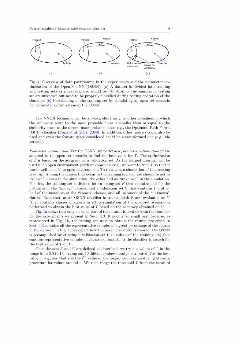
Fig. 1: Overview of data partitioning in the experiments and the parameter op-timization of the Open-Set NN (OSNN). (a) A dataset is divided into trainingand testing sets as a real scenario would be. (b) Most of the samples in testingset are unknown but need to be properly classified during testing operation of theclassifier. (c) Partitioning of the training set by simulating an open-set scenariofor parameter optimization of the OSNN.

The NNDR technique can be applied, effortlessly, to other classifiers in whichthe similarity score to the most probable class is smaller than or equal to thesimilarity score to the second most probable class, e.g., the Optimum-Path Forest(OPF) classifier (Papa et al. 2007, 2009). In addition, other metrics could also beused and even the feature space considered could be a transformed one (e.g., viakernels).

Parameter optimization. For the OSNN, we perform a parameter optimization phaseadapted to the open-set scenario to find the best value for T . The optimizationof T is based on the accuracy on a validation set. As the learned classifier will beused in an open environment (with unknown classes), we want to tune T so that itworks well in such an open environment. To that aim, a simulation of that settingis set up. Among the classes that occur in the training set, half are chosen to act as“known” classes in the simulation, the other half as “unknown” in the simulation.For this, the training set is divided into a fitting set F that contains half for theinstances of the “known” classes, and a validation set V that contains the otherhalf of the instances of the “known” classes, and all instances of the “unknown”classes. Note that, as an OSNN classifier is trained with F and evaluated on V

(that contains classes unknown in F ), a simulation of the open-set scenario isperformed to obtain the best value of T based on the accuracy obtained on V .

Fig. 1a shows that only an small part of the dataset is used to train the classifierfor the experiments we present in Sect. 4.3. It is only an small part because, asrepresented in Fig. 1b, the testing set used to obtain the results presented inSect. 4.3 contains all the representative samples of a great percentage of the classesin the dataset. In Fig. 1c we depict how the parameter optimization for the OSNNis accomplished by creating a validation set V (a subset of the training set) thatcontains representative samples of classes not used to fit the classifier to search forthe best value of T on V .

Once the sets F and V are defined as described, we try out values of T in therange from 0.5 to 1.0, trying out 10 different values evenly distributed. For the bestvalue v, e.g., say that v is the ith value in the range, we make another grid search

procedure for values around v. We then range the threshold T from the mean of


the (i − 1)th and ith values to the mean of ith and (i + 1)th values trying out 10different values evenly distributed. We then repeat this refinement procedure infour levels.

The accuracy obtained on the unknown samples, during the performed sim-ulation, can be seen as an estimation of the open space risk RO in Eq. (1). Tothe best of our knowledge, our proposed method is the first to estimate RO basedon data. We present experiments regarding the parameter optimization phase inSection 4.4.

4 Experiments and validation

In this section, we present the evaluation measures (Sect. 4.1) and the experimentalsetup for validating the different methods (Sect. 4.2), including: details of theimplementation of baseline classifiers, the datasets used for validation, and theexperimental protocol. Then, we present the main experiments and the obtainedresults (Sect. 4.3) and experiments towards the evaluation of the parameter settingof the proposed method (Sect. 4.4). Finally, we further discuss the failing cases ofOSNN (Sect. 4.5).

4.1 Evaluation measures

For evaluating classifiers in an open-set scenario, we should be aware of the un-known classes. Most of the existing evaluation measures, such as the macro- andmicro-averaging f-measure, the average accuracy (Sokolova and Lapalme 2009),and the traditional classification accuracy (Chang and Lin 2011), do not takeinto account the unknown. Therefore, another contribution of this paper is theadaptation of two evaluation measures to assess the quality of open-set classifiers.

In the literature, the following classes of evaluation measures are found:(1) Measures for binary closed-set problems (traditional classification accuracy,f-measure, etc.); (2) Measures for multiclass closed-set problems (traditional clas-sification accuracy, multiclass version of the f-measure, etc); and (3) Measures forbinary open-set problems (Costa et al. 2014, the open-set version of the averageaccuracy). Measures in (1) and (2) are not appropriate as they do not consideropen-set scenarios, which usually lead to the overestimation of the performanceof evaluated classifiers. The measures adopted in (3), in turn, do not considermulticlass open-set classification problems.

In this work, we consider the open-set scenario potentially a multiclass scenario,i.e., one would want to classify a test sample as unknown or one of the knownclasses. Under those circumstances, the measures discussed in this work definea new class of evaluation measures, as they are suitable for multiclass open-set

classification problems.Here, we refer to the known samples as the samples belonging to one of the

available classes for training. The unknown samples belong to classes for which norepresentative sample is used during training.

Normalized accuracy. The normalized accuracy (NA) takes into account both theaccuracy on known samples (AKS) and the accuracy on unknown samples (AUS). It


was proposed because it avoids overestimating the performance of biased classifiers,i.e., classifiers that occasionally classify almost all samples as belonging to the mostfrequent class. This is important because the more open the scenario, the greaterthe amount of unknown samples.

The NA is defined as follows.

NA = λrAKS + (1− λr)AUS (4)

in which λr, 0 < λr < 1, is a regularization constant. Note that λr regulates thetradeoff of mistakes on the known and unknown cases. The NA differs from theaccuracy presented by Costa et al. (2014) because the NA is the accuracy of themulticlass problem while the final accuracy in the work of Costa et al. (2014) isthe average of the accuracies obtained in the binary problems.

Open-set f-measure. Besides using the NA to assess the quality of results of classi-fiers in open-set scenarios, we also use extensions of the macro- and micro-averagingf-measure because these measures can give us fine-grained analysis of the behav-ior of the evaluated methods. The definition and the properties of f-measure arepresented by Sokolova and Lapalme (2009). The following equation describes thetraditional f-measure:

f-measure =2× precision× recall

precision + recall(5)

A trivial extension of f-measure to open-set scenario could be to consider theunknown as one simple class and obtain the f-measure value in the same way it isaccomplished for the multiclass closed-set scenario. However, this trivial extensionis not appropriate to evaluate tests in open-set scenarios because all correct classi-fication of unknown test samples would be considered true positive classifications.These classification results cannot be considered true positive because it does notmake sense to consider the unknown classes as one single positive class, since wehave no representative samples of unknown classes to train the classifier.

Our open-set modifications to the f-measure are related to how precision andrecall are computed. Eq. (6) and (7) are used to compute the macro-averaging

open-set f-measure (OSFMM ) and the micro-averaging open-set f-measure (OSFMµ),respectively. The measures precisionM and recallM stand for the macro precisionand the macro recall, respectively. The measures precisionµ and recallµ, in turn,stand for the micro precision and the micro recall, respectively. The following equa-tions detail the proposed modified measures, which are the basis for the f-measurecomputed by Eq. (5) to define the open-set f-measure (OSFM):

precisionM =

∑l−1i=1

TPiTPi+FPil − 1

, recallM =

∑l−1i=1

TPiTPi+FNi

l − 1, (6)

precisionµ =

∑l−1i=1 TPi∑l−1

i=1(TPi + FPi), recallµ =

∑l−1i=1 TPi∑l−1

i=1(TPi + FNi), (7)

in which l = n + 1 is the size of the confusion matrix (represented in Fig. 2) andn is the number of available classes for training. TP, FP, and FN stand for truepositive, false positive, and false negative samples, respectively. For these formulas,the last column and the last row of the confusion matrix refer to the unknown.


1

1

2 3 U

2

3

U

TP1 FN1

FP1

FP1

FP1

FN1 FN1

(a)

1

1

2 3 U

2

3

U

TP2FN2

FP2

FN2 FN2

FP2

FP2

(b)

1

1

2 3 U

2

3

U

FN3

FP3

TP3FN3 FN3

FP3

FP3

(c)

Fig. 2: Open-set confusion matrix. Example related to the computation of the pre-cision and recall measures from an open-set confusion matrix with three availableclasses and unknown samples (U). The FNi in the column U and FPi in the rowU account for false unknown and false known, respectively. The cell in the inter-section of column U and row U is not regarded as true positive in the same way itwould be considered by the multiclass closed-set f-measure.

In Eq. (6) and (7), in spite of computing the precision and recall only for the navailable classes, by taking into account the false negative and the false positive,respectively, the FN and FP also consider the false unknown and false known,respectively, as illustrated in Fig. 2.

The f-measure adopted in traditional multiclass classification is invariant tothe true negative (Sokolova and Lapalme 2009), i.e., the f-measure does not takeinto account the samples truly rejected as belonging to the class under considera-tion. Similarly, the proposed OSFM for open-set scenarios is invariant to the trueunknown. But both the false unknown (known samples incorrectly classified asunknown) and the false known (unknown samples incorrectly classified as known)are considered in the OSFM. We adopted this strategy for two reasons: (1) Thef-measure must give importance to classified known samples and (2) The unknownis not a single class but possibly several ones.

Differently from the NA, the OSFM is sensitive to the unbalancing of theclasses.

4.2 Experimental setup

In this section, we present the baselines (Sect. 4.2.1); the datasets considered inthe experiments (Sect. 4.2.2); and the experimental protocol adopted (Sect. 4.2.3)in this work.

4.2.1 Baselines

We compare the OSNN classifier with the multiclass SVM with one-vs-all ap-proach using two types of grid search procedures (SVMMCBIN and SVMMCBIN

ext ); theSVMMCOC proposed by Pritsos and Stamatatos (2013); the DBCMCBIN of Costaet al. (2012, 2014); the 1VS proposed by Scheirer et al. (2013); the WSVM methodof Scheirer et al. (2014); the traditional NN; and the NN using thresholds withtwo types of grid search procedures to find out the threshold (TNN and TNNext).


Besides these classifiers, we consider the OSNNCV as a baseline for comparisonwith OSNN to show the effectiveness of the ability of OSNN to reject farawaysamples.

In addition to the well-known C and γ parameters of the SVM, there are otherconfigurations that influence the behavior of the classifier. According to Changand Lin (2011), there are two possible ways to accomplish the grid search fora multiclass binary-based classifier such as the SVMMCBIN: (1) the external and(2) the internal grid search.4 In the external approach, the grid search is performedin the multiclass level forcing all the binary classifiers to share the same parameters.On the other hand, in the internal grid search, each binary classifier performsits own grid search. According to Chen et al. (2005), considering the one-vs-oneapproach, the external approach obtains parameters not uniformly good to everybinary classifier. In addition, it considers the overall accuracy of the multiclassclassifier. On the other hand, the internal grid search can over-fit the classifier.However, for closed-set, they result in similar accuracy (Chen et al. 2005).

We used both external and internal grid search approaches for SVM in com-parison to the proposed method herein. These approaches are implemented inSVMMCBIN

ext and SVMMCBIN, respectively. Both classifiers use Radial Basis Function(RBF) kernel. Both 1VS and WSVM use the external grid search, according tothe authors. All other SVM-based baselines use the internal grid search.

Regarding the 1VS, recently Scheirer et al. (2013) released a new version of thecode (more efficient) in their website. We use this new version of the code becauseit already has the implementation of the one-vs-all approach.5

The WSVM implementation was also accomplished using the one-vs-all ap-proach. For this baseline, the authors kindly provided an implementation con-taining the multiclass-from-binary version of the classifier.6 Then, we used the Ccode implementation as provided. We fixed the threshold δτ for the CAP modelin WSVM in 0.001, as specified by the authors (Scheirer et al. 2014), and weperformed a grid search in {2−7, 2−6, . . . , 20} for the threshold δR. Regardingthe SVM parameters, we performed grid search for C ∈ {2−5, 2−3, . . . , 215} andγ ∈ {2−15, 2−13, . . . , 23} following the standard protocol in the literature (Changand Lin 2011). In summary, we performed a tridimensional grid search on theparameters C, γ, and δR.

The TNN classifier is simply the NN with a threshold T on the distance to thenearest neighbor. When the distance to the nearest neighbor is greater than T , thetest sample is classified as unknown. In the grid search for T , we try values from 0to√D with 100 linearly separated values, in which D is the number of features of

the dataset. In our experiments, all feature values of the dataset were normalizedbetween 0 and 1 (the same normalization for all classifiers).

In Table 1, we summarize the evaluated methods. We say that a method isopen set when it somehow allows the classification of a test sample as unknown.

4.2.2 Datasets

We performed experiments considering the following six datasets.

4 We defined these names.5 The code is available in http://www.metarecognition.com/openset/ (As of October 2016).6 The code is available in http://www.metarecognition.com/open-set-with-kernels/ (As

of October 2016).

http://www.metarecognition.com/openset/

http://www.metarecognition.com/open-set-with-kernels/


Table 1: General characteristics of the classifiers used in the experiments.

Method Approach Open-set Kernel Grid search

SVMMCBIN One-vs-all 3 RBF InternalSVMMCBIN

ext One-vs-all 3 RBF ExternalSVMMCOC One-class based 3 RBF InternalDBCMCBIN One-vs-all 3 RBF Internal1VS One-vs-all 3 Linear ExternalWSVM One-vs-all 3 RBF ExternalNN Multiclass 7 – –TNN Multiclass 3 – InternalTNNext Multiclass 3 – ExternalOSNNCV Multiclass 3 – –OSNN Multiclass 3 – External

– In the 15-Scenes (Lazebnik et al. 2006) dataset, with 15 classes, the 4,485images were represented by a bag-of-visual-word vector created with soft as-signment (van Gemert et al. 2010) and max pooling (Boureau et al. 2010),based on a codebook of 1,000 Scale Invariant Feature Transform (SIFT; Lowe2004) codewords.

– The 26 classes of the Letter (Frey and Slate 1991; Michie et al. 1994) datasetrepresent the letters of the English alphabet (black-and-white rectangular pixeldisplays). The 20,000 samples contain 16 attributes.

– The Auslan (Kadous 2002) dataset contains 95 classes of Australian Sign Lan-guage (Auslan) signs collected from a volunteer native Auslan signer (Kadous2002). Data was acquired using two Fifth Dimension Technologies (5DT) gloveshardware and two Ascension Flock-of-Birds magnetic position trackers. Thereare 146,949 samples represented with 22 features (x, y, z positions, bend mea-sures, etc).

– The Caltech-256 (Griffin et al. 2007) dataset comprises 256 object classes.The feature vectors consider a bag-of-visual-words characterization approachand contain 1,000 features, acquired with dense sampling, SIFT descriptor forthe points of interest, hard assignment (van Gemert et al. 2010), and averagepooling (Boureau et al. 2010). In total, there are 29,780 samples.

– The ALOI (Geusebroek et al. 2005) dataset has 1,000 classes and 108 sam-ples for each class (108,000 in total). The features were extracted with theBorder/Interior Pixel Classification (BIC; Stehling et al. 2002) descriptor andcontain 128 dimensions.

– The Ukbench (Nist and Stew 2006) dataset comprises 2,550 classes of fourimages each. In our work, the images were represented with BIC descriptor(128 dimensions).

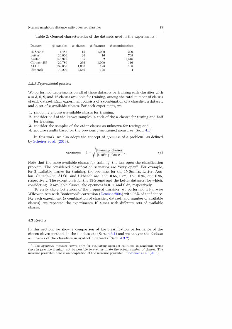
In Table 2, we present the overall characteristics of the datasets we used in theexperiments. Note that we did not try to find the best characterization approachfor each dataset since this is not the focus of this work. We relied on characteristicsthat presented good results according to prior work in the literature. In addition,all of the used features are available on https://dx.doi.org/10.6084/m9.figshare.

1097614.

https://dx.doi.org/10.6084/m9.figshare.1097614

https://dx.doi.org/10.6084/m9.figshare.1097614


Table 2: General characteristics of the datasets used in the experiments.

Dataset # samples # classes # features # samples/class

15-Scenes 4,485 15 1,000 299Letter 20,000 26 16 769Auslan 146,949 95 22 1,546Caltech-256 29,780 256 1,000 116ALOI 108,000 1,000 128 108Ukbench 10,200 2,550 128 4

4.2.3 Experimental protocol

We performed experiments on all of these datasets by training each classifier withn = 3, 6, 9, and 12 classes available for training, among the total number of classesof each dataset. Each experiment consists of a combination of a classifier, a dataset,and a set of n available classes. For each experiment, we

1. randomly choose n available classes for training;2. consider half of the known samples in each of the n classes for testing and half

for training;3. consider the samples of the other classes as unknown for testing; and4. acquire results based on the previously mentioned measures (Sect. 4.1).

In this work, we also adopt the concept of openness of a problem7 as definedby Scheirer et al. (2013).

openness = 1−

√|training classes||testing classes| , (8)

Note that the more available classes for training, the less open the classificationproblem. The considered classification scenarios are “very open”. For example,for 3 available classes for training, the openness for the 15-Scenes, Letter, Aus-lan, Caltech-256, ALOI, and Ukbench are 0.55, 0.66, 0.82, 0.89, 0.94, and 0.96,respectively. The exception is for the 15-Scenes and the Letter datasets, for which,considering 12 available classes, the openness is 0.11 and 0.32, respectively.

To verify the effectiveness of the proposed classifier, we performed a PairwiseWilcoxon test with Bonferroni’s correction (Demsar 2006) with 95% of confidence.For each experiment (a combination of classifier, dataset, and number of availableclasses), we repeated the experiments 10 times with different sets of availableclasses.

4.3 Results

In this section, we show a comparison of the classification performance of thechosen eleven methods in the six datasets (Sect. 4.3.1) and we analyze the decision

boundaries of the classifiers in synthetic datasets (Sect. 4.3.2).

7 The openness measure serves only for evaluating open-set solutions in academic termssince in practice it might not be possible to even estimate the actual number of classes. Themeasure presented here is an adaptation of the measure presented in Scheirer et al. (2013).


SVMMCBIN

SVMMCBINext

SVMMCOC

DBCMCBIN

1VS

WSVM

NN

TNNext

TNN

OSNNCV

OSNN

Normalized accuracy (NA)

12 9 6 3ACS

0.00.20.40.60.81.0

NA

(a) 15-Scenes.

12 9 6 3ACS

0.00.20.40.60.81.0

NA

(b) ALOI.

12 9 6 3ACS

0.00.20.40.60.81.0

NA

(c) Auslan.

12 9 6 3ACS

0.00.20.40.60.81.0

NA

(d) Caltech-256.

12 9 6 3ACS

0.00.20.40.60.81.0

NA

(e) Letter.

12 9 6 3ACS

0.00.20.40.60.81.0

NA

(f) Ukbench.

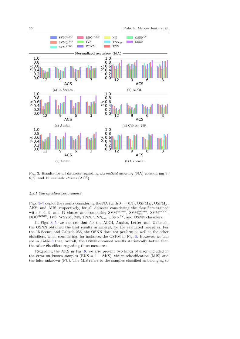
Fig. 3: Results for all datasets regarding normalized accuracy (NA) considering 3,6, 9, and 12 available classes (ACS).

4.3.1 Classification performance

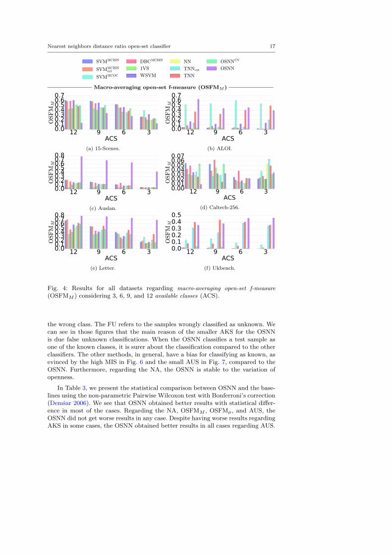
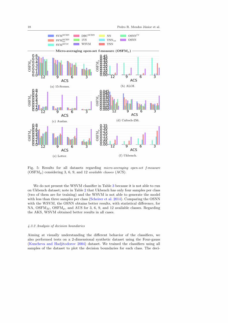
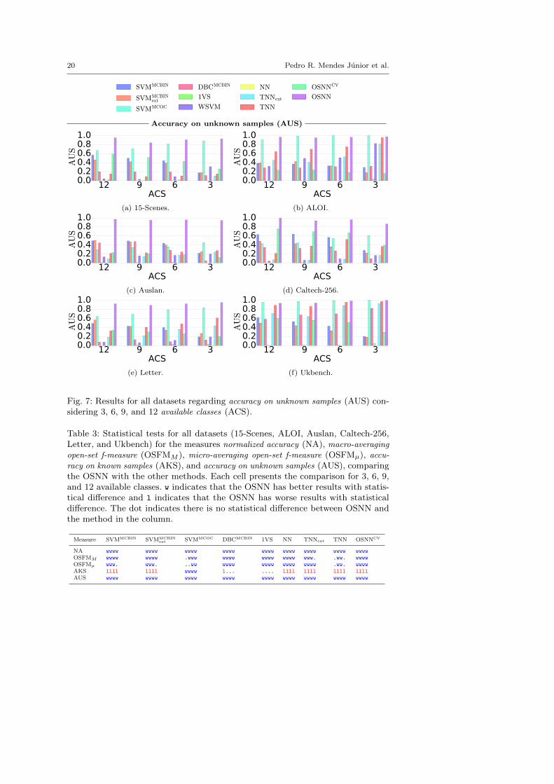
Figs. 3–7 depict the results considering the NA (with λr = 0.5), OSFMM , OSFMµ,AKS, and AUS, respectively, for all datasets considering the classifiers trainedwith 3, 6, 9, and 12 classes and comparing SVMMCBIN, SVMMCBIN

ext , SVMMCOC,DBCMCBIN, 1VS, WSVM, NN, TNN, TNNext, OSNNCV, and OSNN classifiers.

In Figs. 3–5, we can see that for the ALOI, Auslan, Letter, and Ukbench,the OSNN obtained the best results in general, for the evaluated measures. Forthe 15-Scenes and Caltech-256, the OSNN does not perform as well as the otherclassifiers, when considering, for instance, the OSFM in Fig. 5. However, we cansee in Table 3 that, overall, the OSNN obtained results statistically better thanthe other classifiers regarding these measures.

Regarding the AKS in Fig. 6, we also present two kinds of error included inthe error on known samples (EKS = 1 − AKS): the misclassification (MIS) andthe false unknown (FU). The MIS refers to the samples classified as belonging to


SVMMCBIN

SVMMCBINext

SVMMCOC

DBCMCBIN

1VS

WSVM

NN

TNNext

TNN

OSNNCV

OSNN

Macro-averaging open-set f-measure (OSFMM )

12 9 6 3ACS

0.00.10.20.30.40.50.60.7

OSFM

M

(a) 15-Scenes.

12 9 6 3ACS

0.00.10.20.30.40.50.60.7

OSFM

M

(b) ALOI.

12 9 6 3ACS

0.00.10.20.30.40.50.60.70.8

OSFM

M

(c) Auslan.

12 9 6 3ACS

0.000.010.020.030.040.050.060.07

OSFM

M

(d) Caltech-256.

12 9 6 3ACS

0.00.10.20.30.40.50.60.70.8

OSFM

M

(e) Letter.

12 9 6 3ACS

0.00.10.20.30.40.5

OSFM

M

(f) Ukbench.

Fig. 4: Results for all datasets regarding macro-averaging open-set f-measure

(OSFMM ) considering 3, 6, 9, and 12 available classes (ACS).

the wrong class. The FU refers to the samples wrongly classified as unknown. Wecan see in those figures that the main reason of the smaller AKS for the OSNNis due false unknown classifications. When the OSNN classifies a test sample asone of the known classes, it is surer about the classification compared to the otherclassifiers. The other methods, in general, have a bias for classifying as known, asevinced by the high MIS in Fig. 6 and the small AUS in Fig. 7, compared to theOSNN. Furthermore, regarding the NA, the OSNN is stable to the variation ofopenness.

In Table 3, we present the statistical comparison between OSNN and the base-lines using the non-parametric Pairwise Wilcoxon test with Bonferroni’s correction(Demsar 2006). We see that OSNN obtained better results with statistical differ-ence in most of the cases. Regarding the NA, OSFMM , OSFMµ, and AUS, theOSNN did not get worse results in any case. Despite having worse results regardingAKS in some cases, the OSNN obtained better results in all cases regarding AUS.


SVMMCBIN

SVMMCBINext

SVMMCOC

DBCMCBIN

1VS

WSVM

NN

TNNext

TNN

OSNNCV

OSNN

Micro-averaging open-set f-measure (OSFMµ)

12 9 6 3ACS

0.00.10.20.30.40.50.6

OSFM

µ

(a) 15-Scenes.

12 9 6 3ACS

0.000.050.100.150.200.250.300.350.400.45

OSFM

µ

(b) ALOI.

12 9 6 3ACS

0.00.10.20.30.40.50.60.70.8

OSFM

µ

(c) Auslan.

12 9 6 3ACS

0.0000.0050.0100.0150.0200.0250.0300.0350.0400.045

OSFM

µ

(d) Caltech-256.

12 9 6 3ACS

0.00.10.20.30.40.50.60.70.8

OSFM

µ

(e) Letter.

12 9 6 3ACS

0.000.050.100.150.200.250.300.35

OSFM

µ

(f) Ukbench.

Fig. 5: Results for all datasets regarding micro-averaging open-set f-measure

(OSFMµ) considering 3, 6, 9, and 12 available classes (ACS).

We do not present the WSVM classifier in Table 3 because it is not able to runon Ukbench dataset; note in Table 2 that Ukbench has only four samples per class(two of them are for training) and the WSVM is not able to generate the modelwith less than three samples per class (Scheirer et al. 2014). Comparing the OSNNwith the WSVM, the OSNN obtains better results, with statistical difference, forNA, OSFMM , OSFMµ, and AUS for 3, 6, 9, and 12 available classes. Regardingthe AKS, WSVM obtained better results in all cases.

4.3.2 Analysis of decision boundaries

Aiming at visually understanding the different behavior of the classifiers, wealso performed tests on a 2-dimensional synthetic dataset using the Four-gauss(Kuncheva and Hadjitodorov 2004) dataset. We trained the classifiers using allsamples of the dataset to plot the decision boundaries for each class. The deci-


SVMMCBIN

SVMMCBINext

SVMMCOC

DBCMCBIN

1VS

WSVM

NN

TNNext

TNN

OSNNCV

OSNN

Accuracy on known samples (AKS)

12 9 6 3ACS

0.00.20.40.60.81.0

AK

S

(a) 15-Scenes.

12 9 6 3ACS

0.00.20.40.60.81.0

AK

S

(b) ALOI.

12 9 6 3ACS

0.00.20.40.60.81.0

AK

S

(c) Auslan.

12 9 6 3ACS

0.00.20.40.60.81.0

AK

S

(d) Caltech-256.

12 9 6 3ACS

0.00.20.40.60.81.0

AK

S

(e) Letter.

12 9 6 3ACS

0.00.20.40.60.81.0

AK

S

(f) Ukbench.

Fig. 6: Results for all datasets regarding accuracy on known samples (AKS) consid-ering 3, 6, 9, and 12 available classes (ACS). The graphs depicting AKS also depictstwo kinds of error included in the error on known samples (EKS = 1−AKS): themisclassification (MIS) and the false unknown (FU). The MIS and the FU aredepicted in the white and gray bars, respectively.

sion boundary of a class defines the region in which a possible test sample will beclassified as belonging to that class.

In Fig. 8, we present the decision boundaries for the Four-gauss dataset. Basedon these figures, we can note that OSNN (Fig. 8k) successfully bounds the KLOS.While the SVMMCBIN (Figs. 8a and 8b) is able to classify as unknown only thedoubtful samples among the available classes, OSNN also avoids recognizing thefaraway samples. As expected, we can see that SVMMCOC (Fig. 8c) is very special-ized. It makes the classifier obtain a good AUS, however the performance regard-ing the AKS is affected. Overall, its NA (Fig. 3) is also affected. The DBCMCBIN

(Fig. 8d) has a behavior similar to the SVMMCBIN. As it changes the original po-sition of the hyperplane independently for each binary classifier, we can see, inFig. 8d, that the final decision of some binary classifiers predominates over others.


SVMMCBIN

SVMMCBINext

SVMMCOC

DBCMCBIN

1VS

WSVM

NN

TNNext

TNN

OSNNCV

OSNN

Accuracy on unknown samples (AUS)

12 9 6 3ACS

0.00.20.40.60.81.0

AU

S

(a) 15-Scenes.

12 9 6 3ACS

0.00.20.40.60.81.0

AU

S

(b) ALOI.

12 9 6 3ACS

0.00.20.40.60.81.0

AU

S

(c) Auslan.

12 9 6 3ACS

0.00.20.40.60.81.0

AU

S

(d) Caltech-256.

12 9 6 3ACS

0.00.20.40.60.81.0

AU

S

(e) Letter.

12 9 6 3ACS

0.00.20.40.60.81.0

AU

S

(f) Ukbench.

Fig. 7: Results for all datasets regarding accuracy on unknown samples (AUS) con-sidering 3, 6, 9, and 12 available classes (ACS).

Table 3: Statistical tests for all datasets (15-Scenes, ALOI, Auslan, Caltech-256,Letter, and Ukbench) for the measures normalized accuracy (NA), macro-averaging

open-set f-measure (OSFMM ), micro-averaging open-set f-measure (OSFMµ), accu-

racy on known samples (AKS), and accuracy on unknown samples (AUS), comparingthe OSNN with the other methods. Each cell presents the comparison for 3, 6, 9,and 12 available classes. w indicates that the OSNN has better results with statis-tical difference and l indicates that the OSNN has worse results with statisticaldifference. The dot indicates there is no statistical difference between OSNN andthe method in the column.

Measure SVMMCBIN SVMMCBINext SVMMCOC DBCMCBIN 1VS NN TNNext TNN OSNNCV

NA wwww wwww wwww wwww wwww wwww wwww wwww wwwwOSFMM wwww wwww .www wwww wwww wwww www. .ww. wwwwOSFMµ www. www. ..ww wwww wwww wwww wwww .ww. wwwwAKS llll llll wwww l... .... llll llll llll llllAUS wwww wwww wwww wwww wwww wwww wwww wwww wwww


Dataset (a) SVMMCBIN (b) SVMMCBINext (c) SVMMCOC

(d) DBCMCBIN (e) 1VS (f) WSVM (g) NN

(h) TNN (i) TNNext (j) OSNNCV (k) OSNN

Fig. 8: Decision boundaries for the Four-gauss dataset (depicted in the top-leftimage). The non-white regions represent the region in which a test sample wouldbe classified as belonging to the same class of the samples with the same color. Allsamples in the white regions would be classified as unknown.

As expected, the 1VS (Fig. 8e) bounds each class with two hyperplanes, however itmaintains an unbounded KLOS. As the WSVM (Fig. 8f) is based on the OCSVM,we can see a specialized behavior in these figures, however for the high-dimensionaldatasets, the AUS (Fig. 7) is not as good. For the NN (Fig. 8g) classifier, there isno white region, i.e., no test sample is classified as unknown. The TNN and TNNext

(Figs. 8h and 8i) also presented interesting behaviors in the 2-dimensional dataset,however it is well known that in high-dimensional spaces it is difficult to obtain areasonable threshold (Phillips et al. 2011). Finally, we can see that the OSNNCV

(Fig. 8j) is able to classify, as unknown, doubtful test samples, consequently it isnot able to bound the KLOS. In these figures, we can see that most of the baselineclassifiers, including some of the proposed for the open-set scenario (DBCMCBIN

and 1VS), leave an unbounded KLOS.


4.4 Remarks on the OSNN’s parameter optimization

The parameter optimization of the OSNN, described in Sect. 3, performs a simula-tion of the open-set scenario based on the available samples for training to betterestimate the threshold for rejecting unknown samples. In this section, we evaluatesome details about the parameter optimization process. First, in Sect. 4.4.1, weevaluate the influence on the behavior of the OSNN when using a regularizationconstant λr other than 50% for the NA during the parameter optimization process.Then, in Sect. 4.4.2, we evaluate the influence of the amount of classes consideredas unknown during the parameter optimization process.

4.4.1 Influence of the regularization constant

Despite training the OSNN using the NA with λr set to 50%, as shown in theexperiments in Sect. 4.3, we also evaluated the performance of the classifier forsetting λr to 10%, 30%, 70%, and 90%. In Table 4, we compare the OSNN trainedwith λr set to 50% (simply referred to as OSNN) with the OSNN trained withother values of λr (referred to as OSNNλrn, in which n is the percentage set forλr).

As expected, the OSNN obtains better results, with statistical difference in sev-eral cases regarding the NA with λr set to 50%. Interestingly, only the OSNNλr90

classifier obtains worse results with statistical difference for OSFMM and OSFMµ

measures. We can observe the influence of λr during training at the AKS andAUS performances. Remember that λr is proportional to the AKS in Eq. (4).We can see that OSNN obtains better AKS than OSNNλr10 and OSNNλr30 andworse AKS than OSNNλr70 and OSNNλr90. Regarding the AUS, it is the inverse:OSNN obtains worse results than OSNNλr10 and OSNNλr30 and better resultsthan OSNNλr70 and OSNNλr90. Those results on AKS and AUS show that OSNNis sensitive to λr used for training and it can be properly set for training for specificproblems, in case the openness of the problem can be estimated a priori. This isconfirmed in Fig. 9, in which OSNNλr70 and OSNNλr90 have better results in thedataset with small openness (15-Scenes in Fig. 9a; 15 classes) and OSNNλr10 hasbetter results in the dataset with high openness (ALOI in Fig. 9b; 1,000 classes).The results are presented therein for OSFMM , but a similar trend can be observedfor those classifiers when considering OSFMµ as well.

4.4.2 Amount of unknown classes in the simulation

The parameter optimization performed by the OSNN, for the results presentedin Sect. 4.3, relies on a simulation of the open-set scenario by selecting half ofthe available classes for training and considering them as unknown in the fittingset, making it to appear only in the validation set used to estimate the betterthreshold T . Herein, we verify the influence on the classifier for considering otheramounts of the available classes as unknown during the parameter optimization.These experiments were performed only for the open-set scenario considering 12available classes for training. We trained different versions of the OSNN, eachof which selects from 9 to 0 the number of available classes to be considered asunknown. Recall that “0” in this case refers to a closed-set training setup. Werefer to those versions as OSNNn, for n = 0, . . . , 9, in which n is the amount of


OSNNλr10

OSNNλr30

OSNN

OSNNλr70

OSNNλr90

Macro-averaging open-set f-measure (OSFMM )

12 9 6 3ACS

0.00.10.20.30.40.50.6

OSFM

M

(a) 15-Scenes.

12 9 6 3ACS

0.00.10.20.30.40.50.60.7

OSFM

M

(b) ALOI.

Fig. 9: Results for 15-Scenes and ALOI regarding macro-averaging open-set

f-measure (OSFMM ) considering 3, 6, 9, and 12 available classes (ACS) comparingthe OSNN trained with different regularization constant λr during the parameteroptimization phase.



racy on known samples (AKS), and accuracy on unknown samples (AUS), comparingthe OSNN with OSNN trained with regularization constant λr other than 50% dur-ing the parameter optimization. Each cell presents the comparison for 3, 6, 9, and12 available classes. w indicates that the OSNN has better results with statisticaldifference and l indicates that the OSNN has worse results with statistical differ-ence. The dot indicates there is no statistical difference between OSNN and themethod in the column.

Measure OSNNλr10 OSNNλr30 OSNNλr70 OSNNλr90

NA .www .w.w ..w. wwwwOSFMM .... .... .... www.OSFMµ .... .... .... www.AKS wwww wwww llll llllAUS llll llll wwww wwww

the available classes considered as unknown during the parameter optimization.According to our experiments, for all six datasets used in this work, there is nostatistical difference among OSNNn for n = 1, . . . , 9. However, the OSNN0 (thatdoes not simulate the open-set scenario) has worse results with statistical differencecompared to OSNNn for n = 1, . . . , 9 for NA, OSFMM , and OSFMµ in almost allcases. The exception is for OSNN9, that has no statistical difference comparedto OSNN0 for OSFMM and OSFMµ. Regarding the AKS and AUS, the OSNNn

for n = 1, . . . , 9 have statistical difference among them in few cases. The OSNN0,however, obtains better AKS and worse AUS compared to all OSNNn for n =1, . . . , 9 in all cases with statistical difference. In summary, the take-home lessonhere is that it is important to consider at least one of the available classes asunknown during the parameter optimization stage of the OSNN.


With these results, one could wonder whether the OSNN’s effectiveness is onlydue to the open-set simulation performed in its parameter optimization stage andthat using the same parameter optimization for a simple classifier such as TNNwould make it perform similarly to OSNN. To clarify this point, we implementedthe parameter optimization stage for TNNext and compared to the OSNN. Wechose TNNext over TNN because its parameter optimization is designed for externalgrid search as in OSNN. The results show that OSNN outperforms TNNext, withstatistical difference, in virtually all cases considering NA, OSFMM , OSFMµ, andAUS. Only regarding NA for 3 available classes there is no statistical significance. Ifwe consider AKS, their performance is not statistically significant in the majorityof the cases (for 3, 9, and 12 available classes). These results clearly show that theOSNN’s performance is not only due to the parameter optimization stage as onecould think at a first glance.

4.5 Failing cases of OSNN

As we could see in Fig. 6, in general, the OSNN obtained slightly smaller AKScompared to the baselines. This is due to its FU rate, because the OSNN alsoclassifies as unknown a doubtful test sample, i.e., a test sample in the overlappingregion of two or more classes. It happens because the ratio R also approaches 1in such cases. To overcome this problem, we must identify when a test sample isbeing classified as unknown by doubt or because it is faraway from the trainingsamples. In this section, we show some direct approaches trying to differentiatethese two cases.

A first direct approach for this verification is to obtain the typical distance foreach class. In this case, when the OSNN classifies as one of the known classes, thatcasts its final decision. Then when the OSNN classifies as unknown, we compare thedistance from the test sample to the nearest neighbor with the typical distance ofthe nearest neighbor’s class aiming to identify if the test sample is being classifiedas unknown by doubt or because it is faraway from the training samples andprobably belongs to an unknown class. If the distance to the nearest neighboris smaller than or equal to the typical distance of the class, then probably theclassification will be as unknown by doubt. In this case, instead of classifying asunknown, we classify as belonging to the most probable class, i.e., the class of thenearest neighbor. If the distance is greater than the typical distance of the class,it is really considered unknown.

We need to define what would be the typical distance for each class. Below welist some possible reasonable definitions:

Max-Min: For each class, the typical distance is the maximum of the minimumdistances, i.e., for each training sample of the class, we get the distance to itsnearest neighbor and then the maximum of those distances.

Mean-Min: For each class, the typical distance is the mean of the minimum dis-tances, i.e., for each training sample of the class, we get the distance to itsnearest neighbor and then we calculate the mean of those distances.

Median-Min: For each class, the typical distance is the median of the minimumdistances, i.e., for each training sample of the class, we get the distance to itsnearest neighbor and then we calculate the median of those distances.


Dataset (a) OSNNMaxMin (b) OSNNMeanMin (c) OSNNMedMin

(d) OSNNMax (e) OSNNMean (f) OSNNMed (g) OSNN

Fig. 10: Decision boundaries for the Four-gauss dataset (depicted in the top-leftimage). The non-white regions represent the region in which a test sample wouldbe classified as belonging to the same class of the samples with the same color. Allsamples in the white regions would be classified as unknown.

Max: For each class, the typical distance is the maximum of the distances amongthe samples, i.e., we calculate the distance from each sample of the class toeach other sample and then we calculate the maximum of those distances.

Mean: For each class, the typical distance is the mean of the distances among thesamples, i.e., we calculate the distance from each sample of the class to eachother sample and then we calculate the mean of those distances.

Median: For each class, the typical distance is the median of the distances amongthe samples, i.e., we calculate the distance from each sample of the class toeach other sample and then we calculate the median of those distances.

We refer to these extensions of the OSNN classifier that implement the typi-cal distances listed above as OSNNMaxMin, OSNNMeanMin, OSNNMedMin, OSNNMax,OSNNMean, and OSNNMed, respectively.

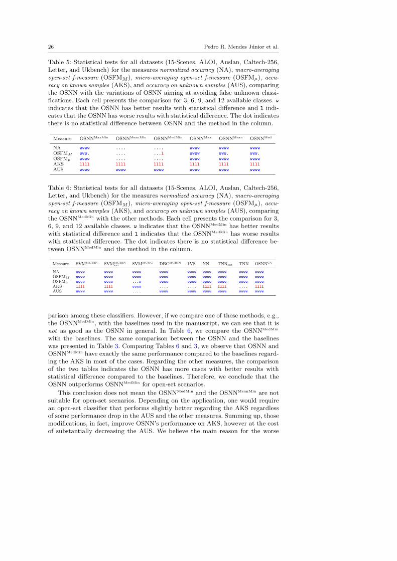
We can see in Table 5 that those modifications are able to improve the AKSwith statistical difference but its performance regarding AUS is worse with sta-tistical difference. We also see that OSNNMeanMin and OSNNMedMin have statisti-cal equivalence with OSNN regarding the NA, OSFMM , and OSFMµ in most ofthe cases. The typical distances considered for the OSNNMeanMin and OSNNMedMin

are the smallest ones compared to the typical distances of the other modifica-tions (OSNNMaxMin, OSNNMax, OSNNMean, and OSNNMed). We can see in Fig. 10that the decision boundaries defined by the OSNNMeanMin (Fig. 10b), OSNNMedMin

(Fig. 10c), and OSNN (Fig. 10g) are similar while the other modifications havegreater changes in their behavior. It means that the additional verification, com-pared to OSNN, takes effect only in a few cases.

One could say that then the OSNNMeanMin or the OSNNMedMin are better thanOSNN because the results presented in Table 5 are not clear regarding the com-




racy on known samples (AKS), and accuracy on unknown samples (AUS), comparingthe OSNN with the variations of OSNN aiming at avoiding false unknown classi-fications. Each cell presents the comparison for 3, 6, 9, and 12 available classes. windicates that the OSNN has better results with statistical difference and l indi-cates that the OSNN has worse results with statistical difference. The dot indicatesthere is no statistical difference between OSNN and the method in the column.

Measure OSNNMaxMin OSNNMeanMin OSNNMedMin OSNNMax OSNNMean OSNNMed

NA wwww .... .... wwww wwww wwwwOSFMM www. .... ...l wwww www. www.OSFMµ wwww .... .... wwww wwww wwwwAKS llll llll llll llll llll llllAUS wwww wwww wwww wwww wwww wwww



racy on known samples (AKS), and accuracy on unknown samples (AUS), comparingthe OSNNMedMin with the other methods. Each cell presents the comparison for 3,6, 9, and 12 available classes. w indicates that the OSNNMedMin has better resultswith statistical difference and l indicates that the OSNNMedMin has worse resultswith statistical difference. The dot indicates there is no statistical difference be-tween OSNNMedMin and the method in the column.

Measure SVMMCBIN SVMMCBINext SVMMCOC DBCMCBIN 1VS NN TNNext TNN OSNNCV

NA wwww wwww wwww wwww wwww wwww wwww wwww wwwwOSFMM wwww wwww wwww wwww wwww wwww wwww wwww wwwwOSFMµ wwww wwww ...w wwww wwww wwww wwww wwww wwwwAKS llll llll wwww .... .... llll llll .... llllAUS wwww wwww .... wwww wwww wwww wwww wwww wwww

parison among these classifiers. However, if we compare one of these methods, e.g.,the OSNNMedMin, with the baselines used in the manuscript, we can see that it isnot as good as the OSNN in general. In Table 6, we compare the OSNNMedMin

with the baselines. The same comparison between the OSNN and the baselineswas presented in Table 3. Comparing Tables 6 and 3, we observe that OSNN andOSNNMedMin have exactly the same performance compared to the baselines regard-ing the AKS in most of the cases. Regarding the other measures, the comparisonof the two tables indicates the OSNN has more cases with better results withstatistical difference compared to the baselines. Therefore, we conclude that theOSNN outperforms OSNNMedMin for open-set scenarios.

This conclusion does not mean the OSNNMedMin and the OSNNMeanMin are notsuitable for open-set scenarios. Depending on the application, one would requirean open-set classifier that performs slightly better regarding the AKS regardlessof some performance drop in the AUS and the other measures. Summing up, thosemodifications, in fact, improve OSNN’s performance on AKS, however at the costof substantially decreasing the AUS. We believe the main reason for the worse


performance, in general, was because we started working with the distance itself(the typical distance comparison) in the Euclidean space instead of only the ratioof distances. Therefore, avoiding the problem of the false unknown of the OSNNis a research topic worth pursuing in the future.

5 Conclusions

Only in the last few years open-set recognition has received the proper attentionand formalization. Usually, experiments in literature are performed consideringthat all classes of the problem are available for training, i.e., a closed-set scenario.However, in real-world situations, the amount of classes during test is many timeslarger than the known classes. That means that real systems must be able to dealwith unknown elements that appear only during the system use and not duringits development. In this work, we have two main contributions:

– The introduction of the Nearest Neighbor Distance Ratio (NNDR)-basedOpen-Set NN (OSNN) classifier; and

– Two new evaluation measures, normalized accuracy (NA) and open-set f-measure

(OSFM), to assess the quality of methods in multiclass open-set recognitionproblems.

The proposed open-set classifier has the advantage of being inherently multi-class (non-binary–based), while the state-of-the-art methods are multiclass frombinary. As more classes are available, multiclass-from-binary classifiers loose someefficiency, while the proposed classifier is not affected by the number of classes.

Based on the results that we presented, we showed that the proposed OSNNoutperforms the baseline classifiers evaluated (SVMMCBIN, SVMMCBIN

ext , SVMMCOC,DBCMCBIN, 1VS, WSVM, NN, TNN, TNNext, and OSNNCV) in most of the casesfor several datasets: 15-Scenes, Letter, Auslan, Caltech-256, ALOI, and Ukbench.We confirmed the superiority of the proposed method using the non-parametricPairwise Wilcoxon test with Bonferroni’s correction (Demsar 2006). As we can seein Fig. 8, the proposed OSNN can gracefully limit the known labeled open space

(KLOS).We showed that OSNN is sensitive to the regularization constant λr estab-

lished for the NA during the parameter optimization, allowing it to be optimizedfor specific open-set problems in case the openness can be estimated a priori. Wealso showed that it is important to perform a simulation of the open-set scenarioduring OSNN’s parameter optimization by leaving at least one of the availableclasses out of the fitting set used to fit an OSNN classifier to estimate the betterthreshold based on the validation set.

The main characteristic of the proposed method is the use of the ratio ofsimilarity scores by applying a threshold on it instead of using the similarity scoreitself. According to our experiments, it is better for bounding the KLOS. Also, theproposed method is stable as the recognition scenario gets more open.

Many of the classifiers in the literature specially proposed for the open-setscenario (SVMMCOC, DBCMCBIN, 1VS, and WSVM) did not obtain good results inour experiments. 1VS and WSVM, for instance, performed worse than traditionalSVM using the one-vs-all approach (SVMMCBIN and SVMMCBIN

ext ), even using thesource code provided by their authors. We observed that the high specialization


of the SVMMCOC makes it obtain a low accuracy on known samples (AKS) and thefinal accuracy is impacted by this behavior.

Future work includes using the proposed parameter optimization for the OSNNas a general open-set grid search procedure and investigating whether this novelgrid search procedure obtains better parameter estimation than the traditionalgrid search for general classifiers.

Another research topic worth pursuing in the future is to extend the NNDRtechnique to consider the ratio not only between the two closest classes to makethe final classification decision. We could consider, for example, 3 or 4 classes andobtain the ratio of similarity score between pairs of these classes. More complexextensions could be investigated using Extreme Value Theory (EVT) (de Haanand Ferreira 2007). The idea is, instead of simply analyzing individual ratio, tocreate a model by fitting an extreme distribution on the smallest ratios. At testing,we could verify if the ratios produced by the test sample belongs or not to thedistribution.

Finally, as we showed in Sect. 4.5, the false unknown (FU) rate obtained bythe OSNN is mainly due to doubtful samples classified as unknown instead of oneof the doubtful classes. We also showed that it is not trivial to identify when thetest sample is being classified as unknown because it is faraway from the trainingsamples or because it is in doubt between two or more training classes. Therefore,future research can also be devoted to investigating meta-recognition approaches(Scheirer et al. 2011, 2012) to develop a classifier to learn when the test sample isbeing classified as unknown by one or another reason.

Acknowledgements Part of the results presented in this paper were obtained through theproject “Pattern recognition and classification by feature engineering, *-fusion, open-set recog-nition, and meta-recognition”, sponsored by Samsung Eletronica da Amazonia Ltda., in theframework of law No. 8248/91. The authors also thank Conselho Nacional de DesenvolvimentoCientıfico e Tecnologico (CNPq; grant #304352/2012-8), Coordenacao de Aperfeicoamento dePessoal de Nıvel Superior (CAPES) through the DeepEyes grant, and Fundacao de Amparoa Pesquisa do Estado de Sao Paulo (FAPESP; grants #2010/05647-4, #2013/50169-1, and#2015/19222-9) for the financial support.

References

Bartlett PL, Wegkamp MH (2008) Classification with a reject option using a hinge loss. Journalof Machine Learning Research 9:1823–1840

Bishop CM (2006) Pattern Recognition and Machine Learning, 1st edn. Information Scienceand Statistics, Springer-Verlag New York

Boureau YL, Bach F, LeCun Y, Ponce J (2010) Learning mid-level features for recognition. In:Intl. Conference on Computer Vision and Pattern Recognition, IEEE Press, San Francisco,CA, pp 2559–2566

Cevikalp H, Triggs B (2012) Efficient object detection using cascades of nearest convex modelclassifiers. In: Intl. Conference on Computer Vision and Pattern Recognition, IEEE Press,Providence, RI, pp 3138–3145

Chang CC, Lin CJ (2011) LIBSVM: A library for support vector machines. Transactions onIntelligent Systems and Technology 2(3):27:1–27:27

Chen PH, Lin CJ, Scholkopf B (2005) A tutorial on nu-support vector machines. AppliedStochastic Models in Business and Industry 21(2):111–136

Chew SW, Lucey S, Lucey P, Sridharan S, Cohn JF (2012) Improved facial expression recogni-tion via uni-hyperplane classification. In: Intl. Conference on Computer Vision and PatternRecognition, IEEE Press, Providence, RI, pp 2554–2561


Chow CK (1970) On optimum recognition error and reject tradeoff. Transactions on Informa-tion Theory 16(1):41–46

Costa FdO, Eckmann M, Scheirer WJ, Rocha A (2012) Open set source camera attribution.In: Conference on Graphics, Patterns, and Images, IEEE Press, Ouro Preto, pp 71–78

Costa FdO, Silva E, Eckmann M, Scheirer WJ, Rocha A (2014) Open set source cameraattribution and device linking. Pattern Recognition Letters 39:92–101

Demsar J (2006) Statistical comparisons of classifiers over multiple data sets. Journal of Ma-chine Learning Research 7:1–30

Dubuisson B, Masson M (1993) A statistical decision rule with incomplete knowledge aboutclasses. Pattern Recognition 26(1):155–165

Frey PW, Slate DJ (1991) Letter recognition using holland-style adaptive classifiers. MachineLearning 6(2):161–182

Fukunaga K (1990) Hypothesis testing. In: Introduction to Statistical Pattern Recognition,2nd edn, Computer Science and Scientific Computing Series, Academic Press, chap 3, pp51–123

van Gemert JC, Veenman CJ, Smeulders AWM, Geusebroek JM (2010) Visual word ambiguity.Transactions on Pattern Analysis and Machine Intelligence 32(7):1271–1283

Geusebroek JM, Burghouts GJ, Smeulders AWM (2005) The amsterdam library of objectimages. Intl Journal of Computer Vision 61(1):103–112

Griffin G, Holub A, Perona P (2007) Caltech-256 object category dataset. Tech. rep., CaliforniaInstitute of Technology

de Haan L, Ferreira A (2007) Extreme value theory: An introduction, 1st edn. Springer Seriesin Operations Research and Financial Engineering, Springer-Verlag New York

Heflin B, Scheirer WJ, Boult TE (2012) Detecting and classifying scars, marks, and tattoosfound in the wild. In: Intl. Conference on Biometrics: Theory, Applications and Systems,IEEE Press, Arlington, VA, pp 31–38

Hodge VJ, Austin J (2004) A survey of outlier detection methodologies. Artificial IntelligenceReview 22(2):85–126

Jayadeva, Khemchandani R, Chandra S (2007) Twin support vector machines for patternclassification. Transactions on Pattern Analysis and Machine Intelligence 29(5):905–910

Jin H, Liu Q, Lu H (2004) Face detection using one-class-based support vectors. In: Intl.Conference on Automatic Face and Gesture Recognition, IEEE Press, Seoul, Korea, pp457–462

Kadous MW (2002) Temporal classification: Extending the classification paradigm to multi-variate time series. PhD thesis, The University of New South Wales, New South Wales,Australia

Kuncheva LI, Hadjitodorov ST (2004) Using diversity in cluster ensembles. In: Intl. Conferenceon Systems, Man and Cybernetics, IEEE Press, The Hague, Netherlands, vol 2, pp 1214–1219

Lazebnik S, Schmid C, Ponce J (2006) Beyond bags of features: Spatial pyramid matching forrecognizing natural scene categories. In: Intl. Conference on Computer Vision and PatternRecognition, IEEE Press, New York, NY, vol 2, pp 2169–2178

Lowe D (2004) Distinctive image features from scale-invariant keypoints. Intl Journal of Com-puter Vision 60(2):91–110

Malisiewicz T, Gupta A, Efros AA (2011) Ensemble of exemplar-svms for object detection andbeyond. In: Intl. Conference on Computer Vision, IEEE Press, Barcelona, pp 89–96

Manevitz LM, Yousef M (2002) One-class svms for document classification. Journal of MachineLearning Research 2:139–154

Michie D, Spiegelhalter DJ, Taylor CC (1994) Machine learning, neural and statistical classi-fication. Ellis Horwood Series in Artificial Intelligence, Prentice Hall, Upper Saddle River,NJ

Muzzolini R, Yang YH, Pierson R (1998) Classifier design with incomplete knowledge. PatternRecognition 31(4):345–369

Nist D, Stew H (2006) Scalable recognition with a vocabulary tree. In: Intl. Conference onComputer Vision and Pattern Recognition, IEEE Press, New York, NY, vol 2, pp 2162–2168

Papa JP, Falcao AX, Miranda PAV, Suzuki CTN, Mascarenhas NDA (2007) Design of robustpattern classifiers based on optimum-path forests. In: Intl. Symposium on MathematicalMorphology, MCT/INPE, Rio de Janeiro, vol 1, pp 337–348


Papa JP, Falcao AX, Suzuki CTN (2009) Supervised pattern classification based on optimum-path forest. Intl Journal of Imaging Systems and Technology 19(2):120–131

Phillips PJ, Grother P, Micheals R (2011) Evaluation methods in face recognition. In: Li SZ,Jain AK (eds) Handbook of Face Recognition, Springer New York, pp 329–348

Pietraszek T (2005) Optimizing abstaining classifiers using roc analysis. In: Intl. Conferenceon Machine learning, ACM Press, Bonn, Germany, pp 665–672

Pritsos DA, Stamatatos E (2013) Open-set classification for automated genre identification.In: Serdyukov P, Braslavski P, Kuznetsov SO, Kamps J, Ruger S, Agichtein E, SegalovichI, Yilmaz E (eds) Advances in Information Retrieval, Lecture Notes in Computer Science,vol 7814, Springer Berlin Heidelberg, pp 207–217

Rocha A, Goldenstein S (2009) Multi-class from binary: Divide to conquer. In: Intl. Conferenceon Computer Vision Theory and Applications, Springer, Lisboa, pp 1–8

Rocha A, Goldenstein S (2014) Multiclass from binary: Expanding one-vs-all, one-vs-oneand ECOC-based approaches. Transactions on Neural Networks and Learning Systems25(2):289–302

Scheirer WJ, Rocha A, Micheals RJ, Boult TE (2011) Meta-recognition: The theory and prac-tice of recognition score analysis. Transactions on Pattern Analysis and Machine Intelli-gence 33(8):1689–1695

Scheirer WJ, Rocha AdR, Parris J, Boult TE (2012) Learning for meta-recognition. Transac-tions on Information Forensics and Security 7(4):1214–1224

Scheirer WJ, Rocha AdR, Sapkota A, Boult TE (2013) Towards open set recognition. Trans-actions on Pattern Analysis and Machine Intelligence 35(7):1757–1772

Scheirer WJ, Jain LP, Boult TE (2014) Probability models for open set recognition. Transac-tions on Pattern Analysis and Machine Intelligence 36(11):2317–2324

Scholkopf B, Platt JC, Shawe-Taylor J, Smola AJ, Williamson RC (1999) Estimating thesupport of a high-dimensional distribution. Tech. rep., Microsoft Research, Redmond, WA

Sokolova M, Lapalme G (2009) A systematic analysis of performance measures for classificationtasks. Information Processing and Management 45(4):427–437

Stehling RO, Nascimento MA, Falcao AX (2002) A compact and efficient image retrievalapproach based on border/interior pixel classification. In: Intl. Conference on Informationand Knowledge Management, ACM Press, McLean, VA, pp 102–109

Wu M, Ye J (2009) A small sphere and large margin approach for novelty detection usingtraining data with outliers. Transactions on Pattern Analysis and Machine Intelligence31(11):2088–2092

Zhou XS, Huang TS (2003) Relevance feedback in image retrieval: A comprehensive review.Multimedia Systems 8(6):536–544

nearest neighbors distance ratio open-set classi er learning manuscript no. (will be inserted by the...

Documents