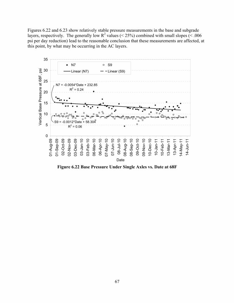
NCAT Report 12-08

FIELD AND LABORATORY STUDY OF HIGH-POLYMER MIXTURES AT THE NCAT TEST TRACK ndash INTERIM REPORT

By Dr David H Timm Mary M Robbins Dr J Richard Willis Dr Nam Tran Adam J Taylor

August 2012

i

Field and Laboratory Study of High-Polymer Mixtures at the NCAT Test Track

Interim Report

By Dr David H Timm Mary M Robbins

Dr J Richard Willis Dr Nam Tran

Adam J Taylor

National Center for Asphalt Technology Auburn University

Sponsored by Kraton Performance Polymers Inc

August 2012

ii

ACKNOWLEDGEMENTS This project was sponsored by Kraton Performance Polymers LLC The project team appreciates and thanks Kraton Performance Polymers LLC for their sponsorship of this project Robert Kluttz of Kraton Performance Polymers LLC deserves special recognition for providing detailed technical and editorial review of this document

DISCLAIMER The contents of this report reflect the views of the authors who are responsible for the facts and accuracy of the data presented herein The contents do not necessarily reflect the official views or policies of Kraton Performance Polymers LLC or the National Center for Asphalt Technology or Auburn University This report does not constitute a standard specification or regulation Comments contained in this paper related to specific testing equipment and materials should not be considered an endorsement of any commercial product or service no such endorsement is intended or implied

iii

TABLE OF CONTENTS

1 INTRODUCTION 1

11 Background 1 12 Objectives and Scope of Work 4

2 INSTRUMENTATION 4 3 MIX DESIGN CONSTRUCTION AND INSTRUMENTATION INSTALLATION 5

31 Mix Design 6 32 Construction and Instrumentation Installation 7

4 LABORATORY TESTING ON BINDERS AND PLANT PRODUCED MIXTURES 20 41 Compaction of Performance Testing Specimens from Plant-Produced Mixes 20 42 Binder Properties 21

421 Performance Grading (AASHTO M 320-10) 21 422 Performance Grading (AASHTO MP 19-10) 21

43 Dynamic Modulus Testing 22 44 Beam Fatigue Testing 30 45 Asphalt Pavement Analyzer (APA) Testing 34 46 Flow Number 36 47 Indirect Tension (IDT) Creep Compliance and Strength 38 48 Energy Ratio 40 49 Moisture Susceptibility 41

5 FALLING WEIGHT DEFLECTOMETER TESTING AND BACKCALCULATION 42 6 PAVEMENT RESPONSE MEASUREMENTS 51

61 Seasonal Trends in Pavement Response 53 62 Pavement Response vs Temperature 56 63 Pavement Responses Normalized to Reference Temperatures 61

631 Longitudinal Strain Responses 62 632 Transverse Strain Responses 63 633 Aggregate Base Vertical Pressure Responses 64 634 Subgrade Vertical Pressure Responses 64

64 Pavement Response Over Time at 68F 65 7 PAVEMENT PERFORMANCE 68 8 KEY FINDINGS CONCLUSIONS AND RECOMMENDATIONS 71 REFERENCES 73 APPENDIX A ndash MIX DESIGN AND AS BUILT AC PROPERTIES 76 APPENDIX B ndash SURVEYED PAVEMENT DEPTHS 83 APPENDIX C ndash BINDER GRADING 85 APPENDIX D ndash MASTER CURVE DATA 90

iv

LIST OF TABLES

Table 31 Mix Design Gradations ndash Percent Passing Sieve Sizes 7 Table 32 Mix Design Parameters 7 Table 33 Random Locations 8 Table 34 Subgrade Dry Unit Weight and Moisture Contents 9 Table 35 Aggregate Base Dry Unit Weight and Moisture Contents 12 Table 36 Date of Paving 14 Table 37 Material Inventory for Laboratory Testing 14 Table 38 Asphalt Concrete Layer Properties ndash As Built 16 Table 41 Summary of Gmm and Laboratory Compaction Temperatures 20 Table 42 Grading of Binders 21 Table 43 Non-Recoverable Creep Compliance at Multiple Stress Levels 22 Table 44 Requirements for Non-Recoverable Creep Compliance (AASHTO MP 19-10) 22 Table 45 Temperatures and Frequencies used for Dynamic Modulus Testing 23 Table 46 High Test Temperature for Dynamic Modulus Testing 23 Table 47 Master Curve Equation Variable Descriptions 25 Table 48 Master Curve Coefficients ndash Unconfined 25 Table 49 Master Curve Coefficients ndash 20 psi Confinement 25 Table 410 Two-Sample t-test p-values (α = 005) comparing Kraton Surface Mix to Control Surface Mix Dynamic Modulus ndash Raw Data 27 Table 411 Two-Sample t-test p-values (α = 005) comparing Kraton IntermediateBase Mix to Control IntermediateBase Mix Dynamic Modulus ndash Raw Data 30 Table 412 Bending Beam Fatigue Results 33 Table 413 Fatigue Curve Fitting Coefficients (Power Model Form) 34 Table 414 Predicted Endurance Limits 34 Table 415 APA Test Results 35 Table 416 Average Measured IDT Strength Data 38 Table 417 Failure Time and Critical Temperature 40 Table 418 Energy Ratio Test Results 41 Table 419 Summary of TSR Testing 42 Table 51 FWD Sensor Spacing 43 Table 52 FWD Drop Heights and Approximate Weights 43 Table 61 Pavement Response vs Temperature Regression Terms 59 Table 62 Predicted Fatigue Life at 68F 63

v

LIST OF FIGURES

Figure 11 Typical Crack Propagation in a Toughened Composite (Scientific Electronic Library Online 2010) 1 Figure 12 Dispersion of SBS Polymer in Asphalt at Different Loadingshelliphelliphelliphelliphelliphelliphelliphelliphellip2 Figure 21 Gauge Array 5 Figure 31 Cross-Section Design Materials and Lift Thicknesses 6 Figure 32 Random Location and Instrumentation Schematic 8 Figure 33 Subgrade Earth Pressure Cell Installation Prior to Final Covering 9 Figure 34 Final Survey of Subgrade Earth Pressure Cell 10 Figure 35 Subgrade and Aggregate Base 11 Figure 36 Surveyed Aggregate Base Thickness 12 Figure 37 Gauge Installation (a) Preparing grid and laying out gauges (b) Trench preparation (c) Gauges placed for paving (d) Placing protective cover material over each gauge (e) Paving over gauges 13 Figure 38 Mixture Sampling for Lab Testing 15 Figure 39 N7 Measured and Predicted Cooling Curves (Lifts 1 2 and 3) 17 Figure 310 S9 Measured and Predicted Cooling Curves (Lifts 1 2 and 3) 17 Figure 311 Average Lift Thicknesses and Depth of Instrumentation 18 Figure 312 Temperature Probe Installation 19 Figure 313 Asphalt Strain Gauge Survivability 19 Figure 41 IPC Global Asphalt Mixture Performance Tester 23 Figure 42 Confined Dynamic Modulus Testing Results ndash 95 mm NMAS Mixtures 26 Figure 43 Unconfined Dynamic Modulus Testing Results ndash 95 mm NMAS Mixtures 27 Figure 44 Confined Dynamic Modulus Testing Results ndash 19 mm NMAS Mixtures 28 Figure 45 Unconfined Dynamic Modulus Testing Results ndash 19 mm NMAS Mixtures 29 Figure 46 Kneading Beam Compactor 31 Figure 47 IPC Global Beam Fatigue Testing Apparatus 31 Figure 48 Comparison of Fatigue Resistance for Mixtures 33 Figure 49 Asphalt Pavement Analyzer 35 Figure 410 Rate of Rutting Plot 36 Figure 411 Flow Number Test Results 37 Figure 412 Indirect Tension Critical Analysis Data 40 Figure 51 Dynatest Model 8000 FWD 43 Figure 52 Backcalculated AC Modulus vs Date (Section-Wide Average) 44 Figure 53 Backcalculated Granular Base Modulus vs Date (Section-Wide Average) 45 Figure 54 Backcalculated Subgrade Soil Modulus vs Date (Section-Wide Average) 45 Figure 55 Backcalculated AC Modulus vs Mid-Depth Temperature (RMSElt3) 47 Figure 56 N7 Backcalculated AC Modulus vs Mid-Depth Temperature RMSE Comparison 48 Figure 57 Backcalculated AC Modulus Corrected to Reference Temperatures 49 Figure 58 Backcalculated AC Modulus vs Date at 68oF (RMSE lt 3) 50

vi

Figure 59 Backcalculated AC Modulus (N7) vs Date at 68oF (No RMSE Restriction) 51 Figure 61 DaDISP Screen Capture of Pressure Measurements for Truck Pass 52 Figure 62 DaDISP Screen Capture of Longitudinal Strain Measurements 53 Figure 63 DaDISP Screen Capture of Transverse Strain Measurements 53 Figure 64 Longitudinal Microstrain Under Single Axles 54 Figure 65 Transverse Microstrain Under Single Axles 55 Figure 66 Aggregate Base Pressure Under Single Axles 55 Figure 67 Subgrade Pressure Under Single Axles 56 Figure 68 Longitudinal Strain vs Mid-Depth Temperature Under Single Axles 57 Figure 69 Transverse Strain vs Mid-Depth Temperature Under Single Axles 57 Figure 610 Base Pressure vs Mid-Depth Temperature Under Single Axles 58 Figure 611 Subgrade Pressure vs Mid-Depth Temperature Under Single Axles 58 Figure 612 Longitudinal Strain vs Mid-Depth Temperature Under Single Axles (N7 ndash 2172010 Cutoff) 59 Figure 613 Transverse Strain vs Mid-Depth Temperature Under Single Axles (N7 ndash 2172010 Cutoff) 60 Figure 614 Aggregate Base Pressure vs Mid-Depth Temperature Under Single Axles (N7 ndash 2172010 Cutoff) 60 Figure 615 Subgrade Pressure vs Mid-Depth Temperature Under Single Axles (N7 ndash 2172010 Cutoff) 61 Figure 616 Longitudinal Strain Under Single Axles at Three Reference Temperatures 62 Figure 617 Transverse Strain Under Single Axles at Three Reference Temperatures 63 Figure 618 Base Pressure Under Single Axles at Three Reference Temperatures 64 Figure 619 Subgrade Pressure Under Single Axles at Three Reference Temperatures 65 Figure 620 Longitudinal Microstrain Under Single Axles vs Date at 68F 66 Figure 621 Transverse Microstrain Under Single Axles vs Date at 68F 66 Figure 622 Base Pressure Under Single Axles vs Date at 68F 67 Figure 623 Subgrade Pressure Under Single Axles vs Date at 68F 68 Figure 71 Measured Rut Depths 69 Figure 72 Measured IRI 69 Figure 73 Roughness vs Distance in Kraton Section 70

1

1 INTRODUCTION 11 Background (excerpt from Timm et al 2011) Ever increasing traffic intensities and pavement loadings accompanied by depleted agency budgets demand that pavement structures achieve better performance more efficiently to reach an overall reduced life cycle cost Polymer-modified asphalt (PMA) is a well-established product for improving the effectiveness of asphalt pavements In particular styrene-butadiene-styrene (SBS) polymers are commonly used to improve permanent deformation resistance and durability in wearing courses (von Quintus 2005 Anderson 2007) Use of SBS in intermediate and base courses has been limited due partly to the perception that base courses with narrower temperature spans than surface courses do not need modification However the ability of SBS polymers to resist fatigue cracking could in theory be used to reduce the overall cross-section of a flexible pavement This is of particular importance for perpetual pavements that often feature high-modulus intermediate asphalt layers and fatigue-resistant bottom layers There is a need for a material that has enhanced fatigue characteristics and can carry load in a more efficient manner through a reduced cross-section Thermoplastic rubbers are used in a variety of industries to toughen composites and plastics The combination of low modulus high elongation high tensile strength and high fracture energy that rubbers typically exhibit are excellent for inhibiting crack initiation and propagation (Halper and Holden 1988) Figure 11 depicts a micrograph of a propagating crack in a typical rubber-toughened composite

Figure 11 Typical Crack Propagation in a Toughened Composite (Scientific Electronic

Library Online 2010) As a crack propagates through a composite material it follows the path of least resistance avoiding the rubbery tough phase and propagating through the weaker brittle phase If the tough

2

rubbery phase now becomes the dominant phase the propagating crack is trapped or ldquopinnedrdquo and cracking in the composite is greatly reduced The polymer level needed to achieve this sort of phase inversion in a modified asphalt is a critical question While an exact answer depends on the details of the physical and chemical interaction between a specific polymer and a specific asphalt Figure 12 gives a general answer

Figure 12 Dispersion of SBS Polymer in Asphalt at Different Loadings

SBS polymers have a strong interaction with bitumen and absorb up to ten times their own volume of less polar asphalt components (Morgan and Mulder 1995) For example instead of having an asphalt modified with 4 of SBS it is more appropriate to consider the modified binder as one that contains 25 ndash 40 of extended polymer on a volume basis This is depicted in Figure 12 showing the relative proportions of swollen polymer and bitumen and actual micrographs showing the interdispersion of polymer and bitumen phases At a typical modification polymer loading of 25 ndash 3 it is likely that the extended polymer is not yet continuously present in the binder It will improve rutting resistance dramatically and it will also

3

improve the fatigue resistance substantially but there will be a further very significant improvement once the extended polymer is a fully continuous phase Thus it is clear that higher polymer loadings have the potential to take cracking resistance to a much higher level than is normally achieved in polymer-modified asphalts At the same time one would also expect that the increase in elasticity while keeping modulus more or less constant should simultaneously give improvement in permanent deformation resistance This strategy has been used in roofing applications for decades where SBS ldquomod bitrdquo roofing membranes typically contain over 10 polymer based on asphalt and the modified asphalt itself functions as a major structural component of the roof assembly However there is a challenge in formulating binders with such high polymer loadings for paving applications At 7+ polymer in a stiff base asphalt conventional SBS polymers will either give poor compatibility poor workability at conventional mixing and compaction conditions or both Kraton Performance Polymers LLC has developed PMA formulations that have a very high polymer content 7-8 yet have practical compatibility and viscosity for drum plant or pug mill production and for laydown and compaction At this content the polymer forms a continuous network in the asphalt turning it into an elastomer with substantially increased resistance to permanent deformation and fatigue cracking Four-point bending beam fatigue testing on mixtures with these binders has shown well over an order of magnitude increase in fatigue life (van de Ven et al 2007 Molenaar et al 2008 Kluttz et al 2009) In addition 3D finite element modeling using the continuum damage Asphalt Concrete Response (ACRe) model developed by TU Delft (Scarpas and Blaauwendraad 1998 Erkens 2002) predicts improved resistance to permanent deformation and fatigue damage even with a 40 reduction in thickness (Halper and Holden 1988 von Quintus 2005 Anderson 2007) While the laboratory and simulation work done on this highly-polymer-modified (HPM) formulation were promising field trials were necessary to fully understand the in-situ characteristics From a structural design and analysis perspective this is needed to evaluate whether HPM behaves like a conventional material under truck and falling weight deflectometer (FWD) loadings so that it can be modeled with conventional approaches (eg layered elasticity) within mechanics-based design frameworks From a performance perspective field trials were needed to evaluate whether the thickness reduction estimate is viable To meet these needs a full-scale experimental HPM section sponsored by Kraton Performance Polymers LLC was constructed at the National Center for Asphalt Technology (NCAT) Test Track in 2009 A control section was constructed at the same time as part of a pooled fund group experiment The sections were designed to provide comparisons between the HPM and control materials The HPM section was designed to be thinner than the control section to investigate whether equal or better performance could be achieved cost effectively using HPM materials At the writing of this report in June 2011 approximately 89 million standard axle loads had been applied to the sections Though some of the questions regarding longer-term performance will require further traffic and forensic investigation to fully answer some of the issues mentioned above can now be directly addressed using data generated during construction in the laboratory and under dynamic vehicle and falling weight deflectometer (FWD) loading

4

12 Objectives and Scope of Work The objective of this report was to document the findings from the Kraton and control sections at the Test Track after 22 months of testing The findings include data obtained during construction laboratory-determined mechanistic and performance properties deflection testing dynamic strain and pressure measurements in addition to preliminary performance results This report will also serve as a reference document for subsequent documentation of these sections 2 INSTRUMENTATION Central to this investigation were the embedded earth pressure cells asphalt strain gauges and temperature probes installed at different points in the construction process The installation of the gauges will be discussed in the following section on construction while the gauges themselves are discussed in this section Figure 21 illustrates the gauge array used in this investigation The instruments and arrangement were consistent with previous experiments at the Test Track (Timm et al 2004 Timm 2009) to provide continuity and consistency between research cycles Within each section an array of twelve asphalt strain gauges was used to capture strain at the bottom of the asphalt concrete The gauges manufactured by CTL were installed such that longitudinal (parallel to traffic) and transverse (perpendicular to traffic) strains could be measured Two earth pressure cells manufactured by Geokon were installed to measure vertical stress at the asphalt concreteaggregate base interface Temperature probes manufactured by Campbell Scientific were installed just outside the edge stripe to measure temperature at the top middle and bottom of the asphalt concrete in addition to 3 inches deep within the aggregate base Full explanation regarding the sensors and arrangement has been previously documented (Timm 2009)

5

Figure 21 Gauge Array

3 MIX DESIGN CONSTRUCTION AND INSTRUMENTATION INSTALLATION This section documents the mix design production and construction of the Kraton section in addition to the control section at the Test Track Where appropriate gauge installation procedures are also discussed Figure 31 illustrates the as-designed pavement sections The mix types and lift thicknesses are indicated in Figure 31 where the lifts are numbered top-to-bottom (eg 1 = surface mix)

-12

-10

-8

-6

-4

-2

0

2

4

6

8

10

12

-12 -10 -8 -6 -4 -2 0 2 4 6 8 10 12

Transverse Offset from Center of Outside Wheelpath ft

Lon

gitu

din

al O

ffse

t fr

om C

ente

r of

Arr

ay f

t

Earth Pressure CellAsphalt Strain Gauge

Edge StripeOutside WheelpathInside WheelpathCenterline

Direction of Travel

1 2 3

4 5 6

7 8 9

10 11 12

13

14

21

20

19

18

Temperature probe

6

Figure 31 Cross-Section Design Materials and Lift Thicknesses

31 Mix Design A summary of the mix design results are provided here with more details available in Appendix A In subsequent sections details regarding the as-built properties of the mixtures are provided Two design gradations were used in this study The surface layers utilized a 95 mm nominal maximum aggregate size (NMAS) while the intermediate and base mixtures used a 19 mm NMAS gradation The aggregate gradations were a blend of granite limestone and sand using locally available materials Distinct gradations were developed for each control mixture (surface intermediate and base) to achieve the necessary volumetric targets as the binder grade and nominal maximum aggregate size (NMAS) changed between layers The Kraton gradations were very similar to the control mixtures Table 31 lists the gradations by mixture type

0

1

2

3

4

5

6

7

8

9

10

11

12

13

14

De

pth

Be

low

Sur

face

in

Agg Base 6 6

Lift3 225 3

Lift2 225 275

Lift1 125 125

Kraton Control

Kraton Intermediate

Kraton Surface Control Surface

Control Intermediate

Control Base

Aggregate Base

Kraton BaseLift 3

Lift 2

Lift 1

7

Table 31 Mix Design Gradations ndash Percent Passing Sieve Sizes Surface Layer Intermediate Layer Base Layer

Sieve Size mm Control Kraton Control and Kraton Control Kraton 25 100 100 100 100 100 19 100 100 93 93 93

125 100 100 82 84 82 95 100 100 71 73 71 475 78 77 52 55 52 236 60 60 45 47 45 118 46 45 35 36 35 06 31 31 24 25 24 03 16 16 12 14 12 015 10 9 7 8 7 0075 58 57 39 46 39

The mixtures were designed using the Superpave gyratory compactor (SGC) with 80 design gyrations This level of compaction was determined through discussion and consensus with the representative sponsor groups Table 32 lists the pertinent mix design parameters and resulting volumetric properties for each of the five mixtures The control and Kraton mixtures had very similar volumetric properties despite the large difference in binder performance grade (PG) resulting from the additional polymer in the Kraton mixes

Table 32 Mix Design Parameters Mixture Type Control Kraton

Lift (1=surface 2=intermediate 3=base)

1 2 3 1 2 amp 3

Asphalt PG Grade 76-22 76-22 67-22 88-22 88-22 Polymer Modification 28 28 0 75 75

Design Air Voids (VTM) 4 4 4 4 4 Total Combined Binder (Pb) wt 58 47 46 59 46

Effective Binder (Pbe) 51 41 41 53 42 Dust Proportion (DP) 11 09 11 11 09

Maximum Specific Gravity (Gmm) 2483 2575 2574 2474 2570 Voids in Mineral Aggregate (VMA) 158 139 139 162 140

Voids Filled with Asphalt (VFA) 75 71 71 75 72 32 Construction and Instrumentation Installation At the Test Track sections are designated according to their respective tangents (North = N South = S) and section numbers (1 through 13 on each tangent) The Kraton section was placed in N7 while the control section was placed in S9 Section placement was based on availability of sections and for ease of construction

8

Within each test section prior to any construction activities four random longitudinal stations (RLrsquos) were established with three transverse offsets (outside wheelpath (OWP) inside wheelpath (IWP) and between wheelpath (BWP)) at each RL These locations were numbered sequentially from 1 through 12 with each location corresponding to a particular RL and offset Figure 32 shows these locations schematically RL 1 2 and 3 were randomly selected from 50-ft subsections within the center 150 ft of each section Transition areas of 25 ft at either end of each section allow for mixture and elevation changes as needed RL 4 was placed at the center of the instrumentation array within each section Table 33 lists the random location stations for each section These locations were important during construction in that they were the locations of nuclear density testing and survey points for thickness Once traffic began they served as locations for frequent falling-weight deflectometer (FWD) testing and determination of transverse profiles

Figure 32 Random Location and Instrumentation Schematic

Table 33 Random Locations

Random Location N7 (Kraton) S9 (Control) 1 37 32 2 70 114 3 114 139

4 (center of gauges) 101 76 In each section the subgrade was compacted to target density and moisture contents The subgrade was consistent with the materials used in previous research cycles and has been well-

0

1

2

3

4

5

6

7

8

9

10

11

12

0 25 50 75 100 125 150 175 200

Distance From Start of Section ft

Dis

tanc

e fr

om E

dge

Str

ipe

ft

1

2

3

4

5

6

10

11

12

7

8

9

Centerline

Edgestripe

RL1 RL2RL4

(Gauge Array) RL3

IWP

BWP

OWP

FWD surveyed depth and density testing locations

Subsection 1 Subsection 2 Subsection 3

Tra

nsiti

on A

rea

Tra

nsiti

on A

rea

Traffic

EmbeddedInstrumentation

9

documented (Taylor and Timm 2009) The subgrade was classified as an AASHTO A-4(0) metamorphic quartzite soil obtained on-site Table 34 lists the average dry unit weight and moisture content achieved in each section

Table 34 Subgrade Dry Unit Weight and Moisture Contents

Test Section N7 (Kraton) S9 (Control) Average Dry Unit Weight lbft3 1218 1234 Average Moisture Content 938 92

After the subgrade had been brought to proper elevation density and moisture content the subgrade earth pressure cells were installed following previously-established procedures (Timm et al 2004 Timm 2009) Each gauge was installed such that it was nearly flush with the top of the subgrade with sieved subgrade material below and on top of the gauge to prevent stress concentrations or damage from stone contact on the plate surface Figure 33 shows an installed plate without the covering material while Figure 34 shows the final surveyed elevation being determined with only the plate face uncovered After the final survey cover material was hand-placed on the gauge followed by construction of the aggregate base

Figure 33 Subgrade Earth Pressure Cell Installation Prior to Final Covering

10

Figure 34 Final Survey of Subgrade Earth Pressure Cell

Following earth pressure cell installation placement of the dense-graded aggregate base commenced The aggregate base was consistent with that used in previous research cycles and has been well-documented (Taylor and Timm 2009) The aggregate base was a crushed granite material often used in Alabama by the state department of transportation (ALDOT) Figure 35 illustrates the prepared subgrade with a portion of the aggregate base in place A small amount of aggregate base was hand placed on the earth pressure cell to protect it from construction traffic until all the material was placed and compacted

11

Figure 35 Subgrade and Aggregate Base

The design called for 6 inches of aggregate base to be placed in each section Surveyed depths were determined at each of the 12 random locations in each section Figure 36 summarizes the surveyed thicknesses at each location (values are tabulated in Appendix B) The random locations and offsets are noted in the figure and correspond to the numbering scheme in Figure 32 Overall slightly less than 6 inches was placed in each section The fact that 6 inches was not achieved uniformly is less important than knowing exactly what the thicknesses were for the purposes of mechanistic evaluation and backcalculation of FWD data Each section was compacted to target density and moisture contents Table 35 summarizes these data for each section

12

Figure 36 Surveyed Aggregate Base Thickness

Table 35 Aggregate Base Dry Unit Weight and Moisture Contents

Test Section N7 (Kraton) S9 (Control) Average Dry Unit Weight lbft3 1406 1402 Average Moisture Content 41 50

Once the aggregate base was complete work began on installing the asphalt strain gauges and aggregate base earth pressure cell Again previously-established procedures (Timm et al 2004 Timm 2009) were followed in lying out and installing the gauges The sequence of photos in Figure 37 highlights the installation procedure more detail can be found elsewhere (Timm et al 2004 Timm 2009)

0

1

2

3

4

5

6

7

8

1 2 3 4 5 6 7 8 9 10 11 12

Agg

rega

te B

ase

Thi

ckne

ss i

n

Location Number

N7

S9

RL1 RL2 RL3 RL4

IWP

BW

P

OW

P

IWP

BW

P

OW

P

IWP

BW

P

OW

P

IWP

BW

P

OW

P

13

(a) (b)

(c) (d)

(e)

Figure 37 Gauge Installation (a) Preparing grid and laying out gauges (b) Trench preparation (c) Gauges placed for paving (d) Placing protective cover material over each

gauge (e) Paving over gauges

14

Table 36 lists the dates on which each pavement lift was constructed The lifts are numbered from top to bottom of the pavement cross section The gaps in paving dates for the control section reflect construction scheduling since many other sections were also paved during this reconstruction cycle

Table 36 Date of Paving Test Section

Asphalt Layer N7 (Kraton) S9 (Control) Lift 1 (surface) July 22 2009 July 16 2009

Lift 2 (intermediate) July 21 2009 July 14 2009 Lift 3 (base) July 20 2009 July 3 2009

Though the primary purpose of this experiment was to validate and understand the field performance of new paving technologies a secondary objective was to characterize asphalt mixtures using these new technologies in the laboratory To provide materials for testing in the laboratory materials were sampled during the paving operation Before construction a testing plan was developed to determine the amount of material needed per mix design to complete its laboratory characterization This testing plan was used to determine the number of 5-gallon buckets to be filled The testing plan varied depending on the type of mix (base intermediate or surface mix) and the sponsorrsquos requests for particular tests Table 37 provides the tally of buckets sampled for each mix associated with this project Upon completion of material sampling the mix was transferred to an off-site storage facility where it was stored on pallets Also included in Table 37 are the sections and lifts that the bucket samples represented Each unique binder was also sampled in the field during the paving operation One 5-gallon bucket of each liquid binder was sampled from the appropriate binder tank at the plant during the mixture production run At the end of each day the binder was taken back to the NCAT laboratory for testing purposes

Table 37 Material Inventory for Laboratory Testing Mixture

Description Kraton Surface

Kraton Base

Control Surface

Control Intermediate

Control Base

Mixture Sampled

N7-1 N7-3 N5-1 S8-2 S8-3

Number of 5-Gallon Buckets

41 35 42 12 30

Section and Lifts Using

Mix N7-1

N7-2 N7-3

S9-1 S9-2 S9-3

Under ideal circumstances mixture samples would have been taken from a sampling tower from the back of a truck However the amount of material needed to completely characterize each mixture made this sampling methodology impossible to achieve Therefore another sampling methodology was developed to ensure that mixture quality and quantity were maintained throughout the sampling process When the mixtures arrived at the Test Track for paving each truck transferred its material to the material transfer vehicle (MTV) After a sufficient amount of the mixture had been transferred into the paver the MTV placed additional mix into the back of

15

a flatbed truck The mixtures were then taken back to the parking lot behind the Test Trackrsquos on-site laboratory for sampling loading into buckets and long-term storage on pallets (Figure 38)

a) Unloading Mix from Truck b) Sampling Mix

c) Loading Mix into Buckets d) Mix Storage

Figure 38 Mixture Sampling for Lab Testing Table 38 contains pertinent as-built information for each lift in each section As documented by Timm et al (2011) the primary differences between S9 and N7 were the amount of polymer and overall HMA thickness Section N7 contained 75 SBS polymer in each lift while S9 utilized more typical levels of polymer in the upper two lifts with no polymer in the bottom lift The nominal binder PG grade of the HPM mixtures in N7 was PG 88-22 However the formulation was designed to meet mixture toughness criteria (or damage resistance) as determined by beam fatigue and finite element modeling (Erkens 2002 Kluttz et al 2009) rather than a specific Superpave PG binder grade The total HMA thickness in N7 was approximately 14 inches thinner than S9 to evaluate its ability to carry larger strain levels more efficiently The mixing and compaction temperatures listed in Table 38 were arrived at through discussions with the polymer supplier plant personnel and the research team (Timm et al 2011) Test mix was generated at the plant and test strips were paved to determine optimum compaction temperatures As shown in Table 38 the HPM mixtures required higher mixing and generally higher compaction temperatures due to the increased polymer content

16

Table 38 Asphalt Concrete Layer Properties ndash As Built (Timm et al 2011) Lift 1-Surface 2-Intermediate 3-Base

Section N7 S9 N7 S9 N7 S9 Thickness in 10 12 21 28 25 30 NMASa mm 95 95 190 190 190 190

SBS 75 28 75 28 75 00 PG Gradeb 88-22 76-22 88-22 76-22 88-22 67-22 Asphalt 63 61 46 44 46 47

Air Voids 63 69 73 72 72 74 Plant Temp oFc 345 335 345 335 340 325 Paver Temp oFd 307 275 286 316 255 254 Comp Temp oFe 297 264 247 273 240 243

aNominal Maximum Aggregate Size bSuperpave Asphalt Performance Grade

cAsphalt plant mixing temperature dSurface temperature directly behind paver

eSurface temperature at which compaction began Of particular interest in Table 38 were the measured temperatures behind the paver In addition to initial temperature temperatures were monitored over time for each paved lift The purpose was to evaluate whether the Kraton system behaved in a fundamentally-different manner in terms of cooling rates relative to conventional AC The evaluation of temperature was made by measuring surface temperature approximately every three minutes after the mat was placed until final compaction was achieved Simulations of mat cooling were then conducted using relevant input data such as time of day paving date and ambient conditions The simulations were conducted using the MultiCool software which was originally developed in Minnesota (Chadbourn et al 1998) for cold weather conditions and adapted for multilayer conditions in California (Timm et al 2001) Since MultiCool uses fundamental heat transfer equations coupled with assumed material properties significant differences between the measured and predicted cooling rates would signify a material behaving in a fundamentally-different manner or having different heat-transfer properties Further details regarding the temperature investigation are documented elsewhere (Vargas and Timm 2011) while the measured and simulated cooling curves are presented in Figures 39 and 310 for N7 and S9 respectively Based on these data it was concluded that MultiCool provided satisfactory predicted cooling curves for each material tested In fact the MultiCool predictions were somewhat better for the Kraton mixtures than the control mixtures This indicates that the materials are cooling in a similar manner and can be simulated with confidence using the MultiCool software

17

Figure 39 N7 (Kraton) Measured and Predicted Cooling Curves (Lifts 1 2 and 3)

Figure 310 S9 (Control) Measured and Predicted Cooling Curves (Lifts 1 2 and 3)

0

50

100

150

200

250

300

350

0 10 20 30 40 50 60 70 80

Time Minutes

Tem

pera

ture

FLift1MultiCool-Lift1

0

50

100

150

200

250

300

350

0 10 20 30 40 50 60 70 80

Time Minutes

Tem

pera

ture

F

Lift2MultiCool-Lift2

0

50

100

150

200

250

300

350

0 10 20 30 40 50 60 70 80 90

Time Minutes

Tem

pera

ture

F

Lift3MultiCool-Lift3

0

50

100

150

200

250

300

350

0 20 40 60 80 100 120

Time minutes

Tem

pera

ture

F

Lift1

MultiCool-Lift1

0

50

100

150

200

250

300

350

0 20 40 60 80 100 120

Time minutes

Tem

pera

ture

F

Lift2

MultiCool-Lift2

0

50

100

150

200

250

300

350

0 20 40 60 80 100 120

Time minutes

Tem

pera

ture

F

Lift3

MultiCool-Lift3

18

After paving each lift of AC depths at the 12 locations (Figure 32) within each section were surveyed This provided very specific lift thickness information in addition to overall pavement depth Figure 311 summarizes these data by providing average depths for each lift of each section The figure also indicates the three instrument types and their depth of installation More detailed information is contained in Appendix B Overall the sections were constructed very close to their target AC thicknesses (575 inches for N7 7 inches for S9)

Figure 311 Average Lift Thicknesses and Depth of Instrumentation

Soon after paving was complete temperature probes were installed in each section The probes were installed as an array of four thermistors to provide temperature at the pavement surface mid-AC bottom-AC and 3 inches below AC Figure 312 illustrates two parts of the probe installation After the vertical hole had been drilled the probes were coated in roofing asphalt and inserted into the hole The cable was tacked to the bottom of the slot running to the edge of the pavement then run through conduit into the data acquisition box

00

10

20

30

40

50

60

70

80

90

100

110

120

130

140

N7 (Kraton) S9 (Control)

Dep

th B

elow

Sur

face

in

Surface Lift Intermediate Lift Bottom Lift Aggregate Base Soil

Temperature

Horizontal Strain

Vertical Base Pressure

Vertical Subgrade Pressure

19

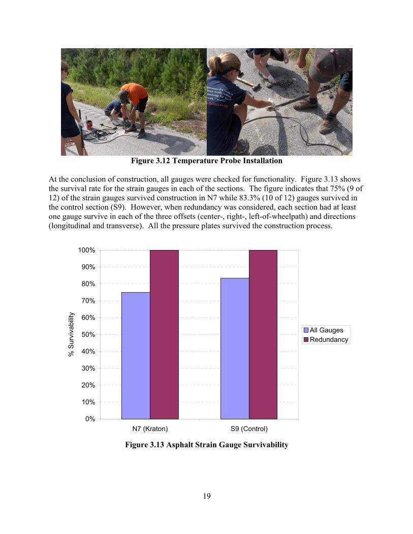
Figure 312 Temperature Probe Installation

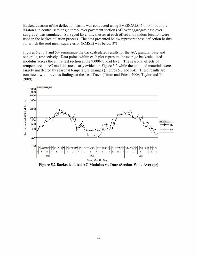
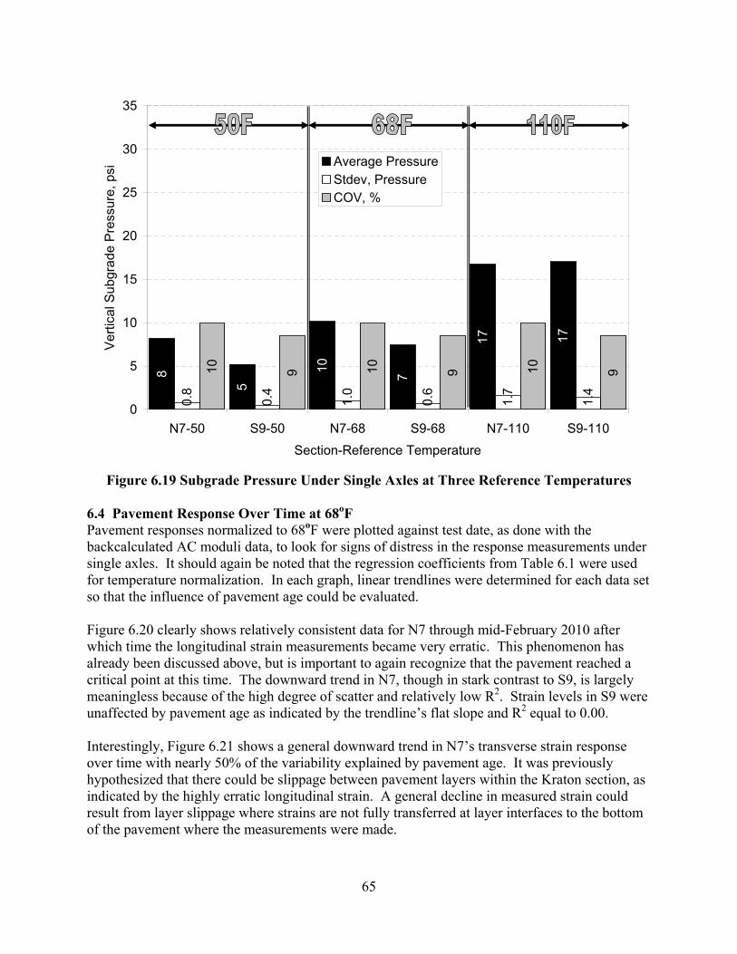
At the conclusion of construction all gauges were checked for functionality Figure 313 shows the survival rate for the strain gauges in each of the sections The figure indicates that 75 (9 of 12) of the strain gauges survived construction in N7 while 833 (10 of 12) gauges survived in the control section (S9) However when redundancy was considered each section had at least one gauge survive in each of the three offsets (center- right- left-of-wheelpath) and directions (longitudinal and transverse) All the pressure plates survived the construction process

Figure 313 Asphalt Strain Gauge Survivability

0

10

20

30

40

50

60

70

80

90

100

N7 (Kraton) S9 (Control)

S

urvi

vabi

lity

All GaugesRedundancy

20

4 LABORATORY TESTING ON BINDERS AND PLANT PRODUCED MIXTURES During production of the mixtures as described previously samples of binder and mix were obtained for laboratory testing and characterization The following subsections detail the tests conducted and results for each mixture and binder 41 Compaction of Performance Testing Specimens from Plant-Produced Mixes For the 2009 research cycle at the Test Track a large amount of plant-produced mix was sampled in order to perform a wide range of laboratory performance tests These mixtures were sampled in 5-gallon buckets and sent to the NCAT laboratory for sample fabrication and testing

The first step in the sample fabrication process was to verify the maximum theoretical specific gravity (Gmm) of each mix in accordance with the AASHTO T209-09 procedure During construction of the Test Track this test was performed on each mix as the mix was constructed The results of these tests are collectively termed ldquoQC Gmmrdquo The test was also performed on the re-heated mix in the NCAT lab For each Kratoncontrol mixture the QC Gmm value and the NCAT lab Gmm fell within the variability allowed by the multi-laboratory precision statement in section 13 of AASHTO T209-09 hence the QC Gmm value was used for sample fabrication

A summary of the Gmm values used for performance sample fabrication can be found in Table 41 The Kraton test section (N7) was constructed in three lifts The base lift and intermediate lift were constructed from the same 19 mm NMAS mix design For the purposes of laboratory testing these mixes were treated as the same The testing on this mix design was performed on mix sampled from the lower lift (lift 3)

Table 41 Summary of Gmm and Laboratory Compaction Temperatures

Mix Description Lab Compaction

Temp F QC Gmm

Lab Gmm

Gmm Difference

Gmm for Lab Samples

Kraton Base and Intermediate

315 2545 2535 0010 2545

Kraton Surface 315 2468 2464 0004 2468 Control Base 290 2540 2538 0002 2540

Control Intermediate 310 2556 2543 0013 2556 Control Surface 310 2472 2464 0008 2472

For sample fabrication the mix was re-heated in the 5-gallon buckets sampled during production at approximately 20oF above the documented lay-down temperature for the Test Track When the mix was sufficiently workable the mix was placed in a splitting pan A quartering device was then used to split out appropriately-sized samples for laboratory testing The splitting was done in accordance with AASHTO R47-08 The individual samples of mix were then returned to an oven set to 10-20oF above the target compaction temperature Once a thermometer in the loose mix reached the target compaction temperature the mix was compacted into the appropriately-sized performance testing sample No short-term mechanical aging (AASHTO R30-02) was conducted on the plant-produced mixes from the test track since these mixes had already been short-term aged during the production process More discussion of sample properties will be provided (sample height target air voids etc) when the individual performance tests are discussed A summary of the target compaction temperatures for this project are provided in Table 41

21

42 Binder Properties Ideally all binders were to be sampled at the plant This was the case for every binder except the virgin asphalt (PG 76-22) used in the surface mixture of S9 The wrong binder was sampled at the plant during construction so this binder was extracted from the surface mixture and the recovered material was tested All the binders used in the two sections were tested in the NCAT binder laboratory to determine the performance grade (PG) in accordance with AASHTO M 320-10 and the performance grade using Multiple Stress Creep Recovery (MSCR) in compliance with AASHTO MP 19-10 Testing results are described in the following subsections

421 Performance Grading (AASHTO M 320-10) The binders were tested and graded according to AASHTO M 320-10 Detailed results are presented in Appendix C Table 42 summarizes the true grade and performance grade of each binder The results confirmed that all the binders used in the construction of the two sections were as specified in the mix designs

Table 42 Grading of Binders Mixture True Grade Performance Grade

All Lifts of N7 (Kraton) 935 ndash 264 88 ndash 22 Base Lift of S9 (Control) 695 ndash 260 64 ndash 22

Intermediate Lift of S9 (Control) 786 ndash 255 76 ndash 22 Surface Lift of S9 (Control) 817 ndash 247 76 ndash 22

Note The binder used in the base lift of Section S9 was graded as PG 67-22 in the southeast It should be noted that while the binder used in N7 had a high temperature performance grade of 88oC and rotational viscosity of 36 PaS its workability and compactability were similar to those of a PG 76-22 binder both in the laboratory and in the field 422 Performance Grading (AASHTO MP 19-10) To determine the performance grade in accordance with AASHTO M 19-10 the MSCR test (AASHTO TP 70-09) was conducted at 64oC which was determined based on the average 7-day maximum pavement design temperature for the Test Track location The MCSR results were used to determine the non-recoverable creep compliance for all the binders The same rolling thin film oven (RTFO) aged specimen utilized in the Dynamic Shear Rheometer (DSR) test according to AASHTO T 315-10 was also used in the MSCR test Table 43 summarizes the MSCR testing results Table 44 shows the acceptable non-recoverable creep compliance at 32 kPa and percent differences for varying levels of traffic as specified in AASHTO MP 19-10 Based on the MSCR test results the virgin binders used in the three layers of Section S9 were graded as PG 64-22 ldquoHrdquo According to AASHTO MP 19-10 high grade ldquoHrdquo is for traffic levels of 10 to 30 million ESALs or slow moving traffic (20 to 70 kmh) The highly polymer-modified binder used in Section N7 was not graded because the percent difference in non-recoverable creep compliance between 01 kPa and 32 kPa (Jnrdiff) was greater than the maximum Jnrdiff specified in AASHTO MP 19-10

22

Table 43 Non-Recoverable Creep Compliance at Multiple Stress Levels

Mixture Test

Temperature Jnr01

(kPa-1) Jnr32

(kPa-1) Jnrdiff

() Performance

Grade All Lifts of N7 64oC 0004 0013 2007 Not Graded Base Lift of S9 64oC 168 195 161 64-22 H

Intermediate Lift of S9 64oC 084 115 369 64-22 HSurface Lift of S9 64oC 098 137 398 64-22 H

Note Jnr01 = average non-recoverable creep compliance at 01 kPa Jnr32 = average non-recoverable creep compliance at 32 kPa

Jnrdiff = percent difference in non-recoverable creep compliance between 01 kPa and 32 kPa

Table 44 Requirements for Non-Recoverable Creep Compliance (AASHTO MP 19-10) Traffic Level Max Jnr32 (kPa-1) Max Jnrdiff ()

Standard Traffic ldquoSrdquo Grade 40 75 Heavy Traffic ldquoHrdquo Grade 20 75

Very Heavy Traffic ldquoVrdquo Grade 10 75 Extremely Heavy Traffic ldquoErdquo Grade 05 75

Note The specified test temperature is based on the average 7-day maximum pavement design temperature 43 Dynamic Modulus Testing Dynamic modulus testing was performed for each of the plant-produced mix types placed during the 2009 Test Track research cycle Due to sampling limitations if a particular mix design was placed in multiple lifts or sections this mix was only sampled one time and tested as representative of that mix type The samples for this testing were prepared in accordance with AASHTO PP 60-09 For each mix three samples were compacted to a height of 170 mm and a diameter of 150 mm and then cut and cored to 150 mm high and 100 mm in diameter All the specimens were prepared to meet the tolerances allowed in AASHTO PP 60-09 The target air void level for the compacted samples is not specified in AASHTO PP 60-09 However the samples were compacted to 7 plusmn 05 air voids which were selected as a common target air void level for pavements compacted in the field Dynamic modulus testing was performed in an IPC Globalreg Asphalt Mixture Performance Tester (AMPT) shown in Figure 41 Dynamic modulus testing was performed to quantify the modulus behavior of the asphalt mixture over a wide range of testing temperatures and loading rates (or frequencies) The temperatures and frequencies used for the Test Track mixes were those recommended in AASHTO PP 61-09 The high test temperature was dependent on the high PG grade of the binder in the mixture Table 45 shows the temperatures and frequencies used while Table 46 shows the selection criteria for the high testing temperature The two Kraton mix designs (surface and base layer) and the control section intermediate course were tested with a high test temperature of 45oC since they were graded as a PG 76-22 or higher The control base course using a PG 64-22 binder was tested at 40oC high test temperature Originally the control surface course using a PG 76-22 binder was tested with a high test temperature of 45oC However due to issues with data quality (deformation drift into tension) the high test temperature was reduced to 40oC as allowed in AASHTO PP 61-09 This vastly improved the quality of data collected while testing that particular mix

23

Figure 41 IPC Global Asphalt Mixture Performance Tester

Table 45 Temperatures and Frequencies used for Dynamic Modulus Testing

Test Temperature (oC) Loading Frequencies (Hz) 4 10 1 01 20 10 1 01

40 (for PG 64-XX) and 45 (for PG 76-XX and higher)

10 1 01 001

Table 46 High Test Temperature for Dynamic Modulus Testing

High PG Grade of Base Binder High Test Temperature (oC) PG 58-XX and lower 35

PG 64-XX and PG 70-XX 40 PG 76-XX and higher 45

Dynamic modulus testing was performed in accordance with AASHTO TP 79-09 This testing was performed both confined and unconfined The confined testing was conducted at 20 psi confining pressure and each compacted specimen was tested at all temperatures and frequencies in the confined mode before proceeding with unconfined testing Test data were screened for data quality in accordance with the limits set in AASHTO TP 79-09 Variability of dynamic modulus values at specific temperatures and frequencies were checked to have a coefficient of variation (COV) at or below 13 All data were checked for reasonableness as well (reduction in moduli with increasing temperature slower loading) Data with borderline data quality statistics were evaluated on a case by case basis The collected data were used to generate a master curve for each individual mix The master curve uses the principle of time-temperature superposition to horizontally shift data at multiple temperatures and frequencies to a reference temperature so that the stiffness data can be viewed

24

without temperature as a variable This method of analysis allows for visual relative comparisons to be made between multiple mixes A reference temperature of 20C was used for this study Generation of the master curve also allows for creation of the dynamic modulus data over the entire range of temperatures and frequencies required for mechanistic-empirical pavement design using the MEPDG By having an equation for the curve describing the stiffness behavior of the asphalt mix both interpolated and extrapolated data points at various points along the curve can then be calculated The temperatures and frequencies needed as an input for the MEPDG are listed in Section 1061 of AASHTO PP 61-09 Also it must be noted that only unconfined master curve data should be entered into the MEPDG since calibration of the design system was originally based on unconfined master curves Data analysis was conducted per the methodology in AASHTO PP 61-09 The general form of the master curve equation is shown as Equation 41 As mentioned above the dynamic modulus data were shifted to a reference temperature This was done by converting testing frequency to a reduced frequency using the Arrhenius equation (Equation 42) Substituting Equation 42 into 41 yields the final form of the master curve equation shown as Equation 43 The shift factors required at each temperature are given in Equation 44 (the right-hand portion of Equation 42) The limiting maximum modulus in Equation 43 was calculated using the Hirsch Model shown as Equation 45 The Pc term Equation 46 is simply a variable required for Equation 45 A limiting binder modulus of 1 GPa was assumed for this equation Data analysis was performed in the MasterSolverreg program developed under the NCHRP 9-29 research project This program uses non-linear regression to develop the coefficients for the master curve equation Typically these curves have an SeSy term of less than 005 and an R2 value of greater than 099 Definitions for the variables in Equations 41-46 are given in Table 47

| lowast| (41)

∆

(42)

| lowast| ∆

(43)

log ∆

(44)

| lowast| 4200000 1 435000 lowast

(45)

(46)

25

Table 47 Master Curve Equation Variable Descriptions Variable Definition

|E| Dynamic Modulus psi δβ and γ Fitting Parameters

Max Limiting Maximum Modulus psi fr Reduced frequency at the reference temperature Hz f The loading frequency at the test temperature Hz

ΔEa Activation Energy (treated as a fitting parameter) T Test Temperature oK Tr Reference Temperature oK

a(T) The shift factor at Temperature T |E|max The limiting maximum HMA dynamic modulus psi VMA Voids in Mineral Aggregate VFA Voids filled with asphalt

The dynamic modulus results for both the Kraton and control sections at the Test Track are documented in the following paragraphs Five plant-produced mix types were tested It should be noted that the base and intermediate courses for section N7 were from the same 19 mm NMAS mix design Therefore for laboratory testing the base-lift material was sampled and tested as representative of both materials Appendix D contains the complete dynamic modulus data set that is required for conducting an MEPDG analysis with these mixes Tables 48 and 49 show the regression coefficients and fitting statistics for the individual master curves for the unconfined and confined tests respectively The fitting statistics for each mix tested (in both a confined and unconfined state) indicate a very high quality of curve fit for both the Kraton and control mixtures Hence it can be inferred that the high level of polymer modification does not negatively impact the dynamic modulus master curve fitting process

Table 48 Master Curve Coefficients ndash Unconfined Mix ID |E|max ksi ksi EA R2 SeSy

Surface-Control 305715 620 -0799 -0484 1987575 0995 0050Surface - Kraton 306992 477 -1336 -0409 2127777 0997 0038

Intermediate-Control 318949 886 -1246 -0472 1988271 0997 0038Base-Control 317754 652 -1086 -0522 1782095 0992 0063

IntermediateBase-Kraton 317123 886 -1064 -0504 1998644 0998 0031

Table 49 Master Curve Coefficients ndash 20 psi Confinement Mix ID |E|max ksi ksi EA R2 SeSy

Surface-Control 305715 6292 -0118 -0560 1911883 0994 0053Surface-Kraton 306992 6182 -0657 -0467 2117241 0997 0039

Intermediate-Control 318949 9093 -0491 -0549 2027477 0997 0039Base-Control 317754 7756 -0321 -0602 1798020 0994 0056

IntermediateBase-Kraton 317123 8464 -0311 -0587 2019217 0996 0043

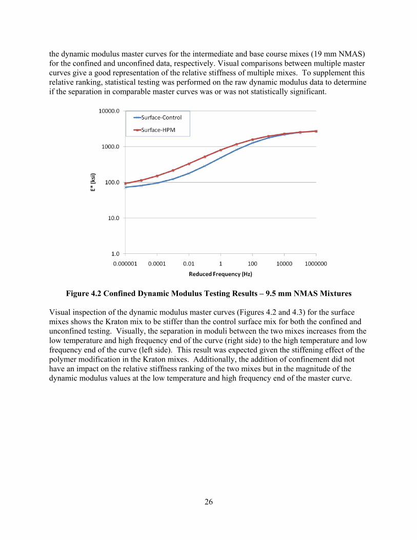
Figures 42 and 43 compare the dynamic modulus master curves for the surface mixes (95 mm NMAS) for both the confined and unconfined data respectively Figures 44 and 45 compare

26

the dynamic modulus master curves for the intermediate and base course mixes (19 mm NMAS) for the confined and unconfined data respectively Visual comparisons between multiple master curves give a good representation of the relative stiffness of multiple mixes To supplement this relative ranking statistical testing was performed on the raw dynamic modulus data to determine if the separation in comparable master curves was or was not statistically significant

Figure 42 Confined Dynamic Modulus Testing Results ndash 95 mm NMAS Mixtures

Visual inspection of the dynamic modulus master curves (Figures 42 and 43) for the surface mixes shows the Kraton mix to be stiffer than the control surface mix for both the confined and unconfined testing Visually the separation in moduli between the two mixes increases from the low temperature and high frequency end of the curve (right side) to the high temperature and low frequency end of the curve (left side) This result was expected given the stiffening effect of the polymer modification in the Kraton mixes Additionally the addition of confinement did not have an impact on the relative stiffness ranking of the two mixes but in the magnitude of the dynamic modulus values at the low temperature and high frequency end of the master curve

27

Figure 43 Unconfined Dynamic Modulus Testing Results ndash 95 mm NMAS Mixtures

To determine if the separation between the two curves was statistically significant a two-sample t-test (α = 005) was performed comparing the test data for the control and Kraton surface mixes This statistical test compared the data for both the confined and unconfined mixes at the different testing temperatures and frequencies A summary of the p-values from these t-tests is given in Table 410 Recall that the high temperatures selected for dynamic modulus testing were different for the control and Kraton mixtures Therefore the 40oC and 200oC temperatures were used to gage whether or not there was a statistical separation between the two curves The p-values given in Table 410 show a strong evidence of a statistical difference in the dynamic modulus data for the control and Kraton mixes at the low and intermediate test temperatures As such this confirms the visual observations in Figures 43 and 44 that the stiffness of the Kraton surface mix is statistically higher than that of the control surface mix

Table 410 Two-Sample t-test p-values (α = 005) comparing Kraton Surface Mix to Control Surface Mix Dynamic Modulus ndash Raw Data

Test Temperature (oC)

Test Frequency (Hz)

p-value of Two Sample t-test Confined (20 psi)

Unconfined (0 psi)

4 01 00003 00012 4 1 00005 00012 4 10 00033 00015 20 01 00023 00019 20 1 00014 00011 20 10 00009 00008

28

A similar examination methodology was used to determine if the Kraton intermediate and base course (recall that the same mix design was used in the lower two lifts of section N7 but only the base lift was sampled for testing purposes) provided a tangible stiffness benefit over the control intermediate and base courses Visual inspection of the confined dynamic modulus testing results (Figure 44) appears to suggest that the intermediate control mix has a higher stiffness than the Kraton 19mm NMAS mix and control base mix at the high temperature and low loading frequency portion of the curve A similar trend is witnessed in the unconfined data (Figure 45) in which the Kraton base mix appears to outperform the control base course at the high temperature and low loading frequency portion of the curve

Figure 44 Confined Dynamic Modulus Testing Results ndash 19 mm NMAS Mixtures

29

Figure 45 Unconfined Dynamic Modulus Testing Results ndash 19 mm NMAS Mixtures Table 411 shows the results of two-sample t-tests (α = 005) that compare the Kraton IntermediateBase mix to both the control intermediate lift and the control base course The data in Table 411 confirms that there is no evidence of a statistical difference between the stiffness of the control base and the Kraton-modified base at the 40oC and 200oC testing temperatures (again no comparisons could be made at the high temperature due to testing protocol) The data in Table 411 also shows there is a statistical difference between the performance of the Kraton-modified intermediate layer and the control intermediate layer with the exception of the data collected at 40oC and 10 Hz Therefore the results show the control intermediate layer had a statistically higher measured stiffness than the Kraton intermediate layer in the dynamic modulus test

30

Table 411 Two-Sample t-test p-values (α = 005) comparing Kraton IntermediateBase Mix to Control IntermediateBase Mix Dynamic Modulus ndash Raw Data

Kraton IntermediateBase versus Control Base

Two Sample t-test p-value

Test Temperature (oC)

Test Frequency (Hz)

Confined (20 psi)

Unconfined

4 01 0161 0477 4 1 0166 0695 4 10 0099 0875 20 01 0266 0079 20 1 0453 0106 20 10 0498 0141

Kraton IntermediateBase versus

Control Intermediate Two Sample t-test p-value

Test Temperature (oC)

Test Frequency (Hz)

Confined (20 psi)

Unconfined

4 01 0019 0009 4 1 0043 0006 4 10 0131 0004 20 01 0002 0003 20 1 0005 0002 20 10 0018 0000 45 001 0003 0016 45 01 0000 0006 45 1 0001 0002 45 10 0003 0000

Overall the collected data suggest that the polymer modification in the Kraton section had a much greater impact on the measured dynamic modulus for the surface courses (95mm NMAS) than that of the intermediate and base courses (19 mm) Little effect was seen on the modulus values at the low temperature and high loading frequency portion of the curve The confinement had significant effects on the modulus magnitudes particularly at the lower reduced frequencies (ie below 1 Hz) At the lowest reduced frequency there was an approximate order of magnitude increase in the dynamic modulus for all mixtures 44 Beam Fatigue Testing Bending beam fatigue testing was performed in accordance with AASHTO T 321-07 to determine the fatigue limits of the base mixtures of the Kraton and control sections described in Section 41 Nine beam specimens were tested for each mix Within each set of nine three beams each were tested at 400 and 800 microstrain The remaining three beams for the Kraton mixture were tested at 600 microstrain while the three control mixture beams were tested at 200 microstrain The specimens were originally compacted in a kneading beam compactor shown in Figure 46 then trimmed to the dimensions of 380 plusmn 6 mm in length 63 plusmn 2 mm in width and 50 plusmn 2 mm in

height Tthe orienfor the fa

The beamHz to ma20 plusmn 05Accordinstiffnessenduranc

The beams wtation in wh

atigue testing

m fatigue appaintain a conC At the beng to AASHT Upon findi

ce limit was

Fi

were compacich the beamg

Figu

paratus shownstant level oeginning of eTO T 321-07ing the cyclecalculated fo

igure 47 IP

cted to a targms were com

ure 46 Knea

wn in Figureof strain at theach test the7 beam failues to failure or each mixt

PC Global B

31

get air void lempacted (top

ading Beam

e 47 applieshe bottom of e initial beamure was defiat three diffeture

Beam Fatigu

evel of 7 plusmn 1and bottom)

m Compacto

s haversine lf the specimem stiffness wined as a 50erent strain m

ue Testing A

10 percent ) was marke

r

loading at a en Testing wwas calculate reduction magnitudes

Apparatus

Additionallyd and maint

frequency owas performed at 50th cycin beam the fatigue

y ained

of 10 med at

cle

32

Using a proposed procedure developed under NCHRP 9-38 (Prowell et al 2010) the endurance limit for each mixture was estimated using Equation 47 based on a 95 percent lower prediction limit of a linear relationship between the log-log transformation of the strain levels and cycles to failure All the calculations were conducted using a spreadsheet developed under NCHRP 9-38

Endurance Limit

xxS

xx

nsty

20

0

11ˆ

(47)

where ŷo = log of the predicted strain level (microstrain) tα = value of t distribution for n-2 degrees of freedom = 2131847 for n = 6 with α = 005 s = standard error from the regression analysis n = number of samples = 9

Sxx =

n

ii xx

1

2 (Note log of fatigue lives)

xo = log (50000000) = 769897 x = log of average of the fatigue life results A summary of the bending beam fatigue test results for the plant-produced base layer mixes is presented in Table 412 Figure 48 compares the fatigue cracking resistance of the two mixtures determined based on AASHTO T 321-07 results A power model transfer function ( ) was used to fit the results for each mixture A summary of the model coefficients and R2 values is given in Table 413 There was a significant difference between the magnitude of the intercept (α1) and the slope (α2 ) between the control mixture and the Kraton mixture These differences were 48 and 44 respectively The R2 values for each of the mixes were above 090 showing a good model fit for the dataset

33

Table 412 Bending Beam Fatigue Results

Mix Specimen Microstrain Level Number of Cycles to Failure

Control Base

1 800

7890 2 17510 3 4260 4

400 201060

5 141250 6 216270 7

200 6953800

8 5994840 9 2165480

Kraton Base

1 800

83600 2 20520 3 14230 4

600 287290

5 195730 6 186920 7

400 11510940

8 1685250 9 4935530

Figure 48 Comparison of Fatigue Resistance for Mixtures

34

Table 413 Fatigue Curve Fitting Coefficients (Power Model Form)

Mixture AASHTO T321-07 α1 α2 R2

Control Base 53742 -0214 0969Kraton Base 27918 -0125 0913

The difference between the average fatigue life of the control mixture to that of the Kraton mixture at two strain levels was determined using the failure criteria (50 reduction in beam stiffness) defined by AASHTO 321-07 This information helps evaluate important aspects of the material behavior shown in Figure 48 as follows At the highest strain magnitude the HPM was able to withstand almost 4 times more loading

cycles than the control mixture At 400 the average fatigue life of the Kraton mixture was much better than the control

mixture The average cycles until failure for the control mixture was 186193 while the Kraton mixture averaged 6043907 loading cycles

Table 414 shows the 95 percent one-sided lower prediction of the endurance limit for each of the two mixes tested in this study based on the number of cycles to failure determined in accordance with AASHTO T 321-07 The procedure for estimating the endurance limit was developed under NCHRP 9-38 (Prowell et al 2010) Based on the results shown in Table 415 the Kraton base mixture had a fatigue endurance limit three times larger than the control mixture

Table 414 Predicted Endurance Limits Mixture Endurance Limit (Microstrain)

Control Base 77 Kraton Base 231

45 Asphalt Pavement Analyzer (APA) Testing The rutting susceptibility of the Kraton and control base and surface mixtures were evaluated using the APA equipment shown in Figure 49 Often only surface mixtures are evaluated using the APA For this experiment however it was directed by the sponsor to test the surface mixture in addition to each of the Kraton mixtures For comparison purposes the base control mixture was also evaluated The intermediate control mix was not sampled in sufficient quantities to allow for APA testing since it was not part of the original APA testing plan

35

Figure 49 Asphalt Pavement Analyzer

Testing was performed in accordance with AASHTO TP 63-09 The samples were prepared to a height of 75 mm and an air void level of 7 plusmn 05 percent Six replicates were tested for each mix Typically these samples are tested at the high binder PG grade However for the Test Track a constant testing temperature for all mixes was desired to facilitate relative comparisons between the mixes Therefore the samples were tested at a temperature of 64oC (the 98 percent reliability temperature for the high PG grade of the binder for the control base mix) The samples were loaded by a steel wheel (loaded to 100 lbs) resting atop a pneumatic hose pressurized to 100 psi for 8000 cycles Manual depth readings were taken at two locations on each sample after 25 loading cycles and at the conclusion of testing to determine the average rut depth (Table 415)

Table 415 APA Test Results

Mixture Average Rut Depth mm

StDev mm COVRate of SecondaryRutting mmcycle

Control-Surface 307 058 19 0000140 Control-Base 415 133 32 0000116

Kraton-Surface 062 032 52 00000267 Kraton-Base 086 020 23 00000280

The APA is typically used as a passfail type test to ensure mixtures susceptible to rutting are not placed on heavily trafficked highways Past research at the Test Track has shown that if a mixture has an average APA rut depth less than 55 mm it should be able to withstand at least 10 million equivalent single axle loads (ESALs) of traffic at the Test Track without accumulating more than 125 mm of field rutting Considering this threshold a one-sample t-test (α = 005) showed all four mixtures had average rut depths less than the given threshold Thus the mixtures are not expected to fail in terms of rutting on the 2009 Test Track An ANOVA (α = 005) was conducted on the data and showed statistical differences between rut depth measurements of the four mixtures A Tukey-Kramer statistical comparison (α = 005) was then used to statistically rank or group the mixtures in terms of rutting performance The statistical analysis placed the four mixtures into two different groups The best performing group contained both Kraton mixtures while the two control mixtures were more susceptible to rutting

36

The APA test results are also appropriate for determining a rate of secondary rutting for each mixture Rutting typically occurs in three stages primary secondary and tertiary Primary rutting develops during the early phases of pavement loading due to initial mixture consolidation (ie further compaction) Secondary rutting begins after initial consolidation with a gradual nearly linear increase in rut depth Tertiary rutting represents a shear flow condition The confined state provided by the molds prevents the mixture from truly ever achieving tertiary flow Therefore once the mixture has overcome the stresses induced during primary consolidation it is possible to determine the rate at which secondary rutting occurs The secondary rutting rate was determined in the APA by fitting a power function to the rut depths measured automatically in the APA during testing (Figure 410) The primary consolidation of a sample can be seen as the initial steep line when comparing rut depth to the number of cycles however as the slope of the line decreases the samples move into secondary consolidation The rate of rutting was determined by finding the slope of the power function at the 8000th loading repetition The results of this analysis are also given in Table 416

Figure 410 Rate of Rutting Plot

Of the four mixtures the Kraton surface mixture had the best or smallest rate of rutting This mixture also had the least amount of total rutting during the test The second most resistant mixture in terms of total rutting and rutting rate was the Kraton base mixture This suggests that using the Kraton modified asphalt binder will allow engineers to design both a flexible and rut resistant asphalt mixture 46 Flow Number The determination of the Flow Number (Fn) for the Kraton and control surface and base mixtures was performed using an Asphalt Mixture Performance Tester (AMPT) Flow number testing was conducted on new specimens which had not been tested for dynamic modulus The

00

05

10

15

20

25

30

0 2000 4000 6000 8000 10000

Ru

t Dep

th (m

m)

No of Cycles

Original APA Data

Fitted Data

37

specimens were fabricated as described in section 43 Fn tests were performed at 595degC which is the LTPPBind version 31 50 reliability temperature at the Test Track 20 mm below the surface of the pavement Additionally the specimens were tested using a deviator stress of 87 psi without the use of confinement The tests were terminated when the samples reached 10 axial strain The Francken model (Biligiri et al 2007) shown in Equation 48 was used to determine tertiary flow Non-linear regression analysis was used to fit the model to the test data

)1()( dNbp ecaNN (48)

where εp (N) = permanent strain at lsquoNrsquo cycles N = number of cycles a b c d = regression coefficients Figure 411 compares the average flow number values for each of the four mixtures evaluated One sample of the Kraton surface mixture never achieved tertiary flow therefore this test result was removed from the evaluation and considered an outlier Even with this outlier removed the Kraton surface mixture had the largest flow number The second best performance mixture was the Kraton base mixture With a flow number of 944 its flow number was approximately 576 times greater than the control base mixture

Figure 411 Flow Number Test Results

An ANOVA (α = 005) conducted on the test results showed statistical differences (p = 0004) between the performance of the four mixtures A Tukey-Kramer analysis (α = 005) was conducted to group the mixtures based on flow number performance The Kraton surface mixture had a statistically larger flow number than the three other mixtures (p = 00136) however the other three mixtures were grouped together in terms of flow number performance despite the differences in mixture performance This is likely due to the high variability in the control base mixture flow number results The COV for this mixture was higher than the recommended COV of 20 in AASHTO TP 79-09 However inspection of the data set for the three samples yielded no significant outliers

38

In summary the Kraton surface mixture showed the highest resistance to deformation of the four mixtures While numerical differences were noted between the Kraton base mixture and the two control mixtures the differences were not statistically significant 47 Indirect Tension (IDT) Creep Compliance and Strength The critical cracking temperature where the estimated thermal stress exceeds the tested indirect tensile strength of a mixture can be used to characterize the low temperature cracking performance of asphalt mixtures This type of analysis could be referred to as a ldquocritical temperature analysisrdquo A mixture that exhibited a lower critical cracking temperature than those of other mixtures would have better resistance to thermal cracking Both surface and base mixtures were evaluated using a critical temperature analysis for this study To estimate the thermal stress and measure the tensile strength at failure the indirect tensile creep compliance and strength tests were conducted for three replicates of each mixture as specified in AASHTO T322-07 A thermal coefficient of each mixture was estimated based on its volumetric properties and typical values for the thermal coefficient of asphalt and aggregate This computation is explained in more detail below The IDT system was used to collect the necessary data for the critical cracking temperature analysis The testing was conducted using a Material Testing Systemreg (MTS) load frame equipped with an environmental chamber capable of maintaining the low temperature required for this test Creep compliance at 0deg -10degC and -20degC and tensile strength at -10degC in accordance with AASHTO T322-07 were measured These temperatures are specified as a function of the low temperature PG grade of the binder in AASHTO T322-07 The creep test applies a constant load to the asphalt specimen for 100 seconds while the horizontal and vertical strains are measured on each face of the specimen using on-specimen instrumentation Four samples were prepared for each mixture The first sample was used to find a suitable creep load for that particular mixture at each testing temperature The remaining three samples were used to develop the data set Samples used for the creep and strength tests were 38 to 50 mm thick and 150 mm in diameter Samples were prepared to 7 plusmn 05 air voids Table 416 shows the average measured tensile strengths of the tested mixtures

Table 416 Average Measured IDT Strength Data Indirect Tensile Strength at -

10degC (MPa) Control ndash Surface

Control ndash Base

Kraton ndash Surface

Kraton - Base

471 416 455 527

An ANOVA test (α = 005) showed statistical differences between the IDT strengths of the four mixtures A Tukey-Kramer statistical analysis (α = 005) only grouped two mixtures together in terms of performance the Kraton and control surface mixtures The Kraton base mixture had a statistically greater strength than the other three mixtures while the control base mixture was statistically lower than the rest Theoretical and experimental results indicate that for linear visco-elastic materials the effect of time and temperature can be combined into a single parameter through the use of the time-

39

temperature superposition principle A creep compliance master curve can be generated by shifting creep compliance data at different temperatures into a single curve at a reference temperature The reference temperature is typically the lowest creep compliance temperature (-20C in this case) The relationship between real time t reduced time ζ and shift factor aT are given in Equation 49 ζ = taT (49) An automated procedure to generate the master curve was developed as part of the Strategic Highway Research Program (Buttlar et al 1998) The system requires the measurement of creep compliance test data at three different test temperatures The final products of the system are a generalized Maxwell model (or Prony series) which is several Maxwell elements connected in parallel and temperature shifting factors The generalized Maxwell model and shifting factors are used for predicting thermal stress development of the asphalt mixture due to changes in temperature In addition to thermo-mechanical properties the thermal coefficient of the asphalt mixture must also be estimated The linear thermal coefficient α was estimated for each mixture using the relationship in Equation 410 (Jones et al 1968)

Total

AggAggACmix V

BVBVMA

3

(410)

where αmix = linear coefficient of thermal contraction of the asphalt mixture (1degC) BAC = volumetric coefficient of thermal contraction of the asphalt cement in the solid state (345 x 10-4degC) BAgg = volumetric coefficient of thermal contraction of the aggregate (1 x 10-6degC) VMA = percent volume of voids in mineral aggregate VAgg = percent volume of aggregate in mixture VTotal = 100 percent Based on the above parameters the change in thermal stress for each mixture was estimated at the cooling rate of 10degC per hour starting at 20degC The finite difference solution developed by Soules et al (1987) was used to estimate the thermal stress development based on the Prony Series coefficients and was performed in a MATHCAD program A complete description of the thermal stress analysis procedure can be found in Hiltunen and Roque (1994) and Kim et al (2008) Figure 412 shows the thermal stress development as a function of temperature reduction Table 417 shows the critical temperature and time to failure determined at the point where thermal stress exceeds the tensile strength

Dat

FaiFai

Based onrate than trends arecritical telayer hasbase mixgrade In summbase mixperforminmixtures 48 EnerThe ener(Roque acut from

Figure

ta

lure Time (hlure Temper

n these resultthat of the K

e also seen iemperature ts a critical temxture does no

ary the Kratxture in tensing mixture ahad critical

rgy Ratio (Ergy ratio wasand Buttlar 1gyratory com

e 412 Indire

Table 417

hour) rature (degC)

ts the controKraton base in the criticathan the contmperature 1

ot have a crit

ton binder sele strength cat low tempetemperature

ER) s developed t1992) To qmpacted sam

ect Tension

7 Failure TimControl ndashSurface

464 -264

ol base mixtumixture Thel temperaturtrol base mix7degC higher tical tempera

eemed to imcritical temperatures was es lower than

to assess a mquantify this mples with 7

40

Critical Te

me and Critndash

e Con

Ba4-2

ure seems toe opposite isre analysis Txture by abothan the con

ature below i

mprove the loperature and

the control bn the require

mixturersquos resproperty thr plusmn 05 air v

emperature

tical Tempentrol ndash ase

KS

14 214

o accumulates seen in the The Kraton bout 45degC Thntrol surfaceits low temp

ow-temperatufailure timebase mixture

ed low tempe

sistance to toree 150 mm voids Resil

Analysis D

erature Kraton ndash Surface

447 -247

e thermal str surface mixbase mixturehe Kraton coe mixture Onperature bind

ure crackinge Overall the Both of therature binde

op-down or sm diameter sp

lient modulu

ata

Kraton - Base 461 -261

ress at a fastextures Thesee has a lowerontrol surfacnly the contrder performa

g resistance ohe poorest he Kraton er grade

surface crackpecimens weus creep

er e r e rol ance

of the

king ere

41

compliance and tensile strengths for each mixture were determined at 10degC Equation 411 was used to evaluate the surface cracking performance of the control and surface mixtures

1982

8135

)10462)366(102947(

Dm

SDSCEER

tf

(411)

where ER = energy ratio σ = tensile stress 150 psi D1 and m = resilient modulus power function parameters St = tensile strength MPa DSCEf = dissipated creep strain energy at failure Table 418 summarizes the energy ratio data for the two surface mixtures evaluated The energy ratio values were indicators of cracking performance of the sections due to the two different binders utilized The energy ratio is calculated by analyzing multiple test samples to arrive at a singular value After analyzing these data only slight differences between the ER of the Kraton and control mixtures were found The higher ER for the control surface mixture suggests that it would perform slightly better in terms of surface cracking However statistical analyses could not be conducted on the data due to the final results being aggregated to form one value

Table 418 Energy Ratio Test Results Parameter Control ndash Surface Kraton - Surface m-value 0327 0282 D1 900 x 10-7 708 x 10-7

St (MPa) 251 251 Mr (GPa) 993 923 FE (kJm3) 81 42 DSCEHMA (kJm3) 778 386 Stress (psi) 150 150 a 461 x 10-8 461 x 10-8 DSCEMIN (kJm3) 070 035 ER 1110 1097

Current recommendations suggest that a minimum ER of 195 is needed to resist surface cracking if trafficking is less than 1000000 ESALs per year (Roque et al 2004) While Test Track trafficking is heavier than this level one can see that these mixtures were more than 5 times greater than the required ER 49 Moisture Susceptibility The moisture susceptibility of the four mixtures was determined using AASHTO T 283-07 Six specimens of each mix were compacted to a height of 95 mm and an air void level of 7 plusmn 05 Three conditioned specimens were vacuum saturated to the point at which 70 to 80 percent of the interval voids were filled with water These samples underwent a freeze-thaw cycle as specified by AASHTO T 283-07

42

The indirect tensile strength was determined using a Pine Instrumentsreg Marshall Stability press which loads the samples at a rate of 2 inmin The IDT strength was then calculated based on the failure loading and measured specimen dimensions AASHTO M 323-07 recommends a tensile-strength ratio (TSR) value of 08 and above for moisture resistant mixtures Table 419 gives a summary of the results from the TSR testing of the four mixtures The TSR values for each of the four mixes exceeded the suggested 080 lower limit Table 419 also shows the average splitting tensile strengths for both the control and Kraton mixtures The splitting tensile strengths of both the base and surface Kraton mixtures were greater than those of the control mixtures There was a slight decrease in TSR values for the Kraton surface mixture when compared to the control surface mixture The opposite was true for the Kraton base mixture

Table 419 Summary of TSR Testing Mixture Treatment Average Splitting Tensile Strength (psi) TSRControl ndash Surface

Conditioned 1372 094

Unconditioned 1454 Control ndash

Base Conditioned 1162

086 Unconditioned 1346

Kraton ndash Surface

Conditioned 1971 089

Unconditioned 2221 Kraton ndash

Base Conditioned 2084

088 Unconditioned 2376

Statistical analyses were conducted to compare the splitting tensile strengths of the mixtures in both their conditioned and unconditioned states An ANOVA (α = 005) showed that for both the conditioned and unconditioned tensile strengths statistical differences (p = 0000) were found between the mixtures The Tukey-Kramer statistical analysis (α = 005) grouped the control mixtures together in terms of splitting tensile strengths in both the conditioned (p = 0263) and unconditioned (p = 0836) states The Kraton test results were also statistically equivalent for both the conditioned (p = 0721) and unconditioned (p = 0646) strengths The Tukey-Kramer analyses showed that Kraton mixtures had statistically higher splitting tensile strengths than the control mixtures 5 FALLING WEIGHT DEFLECTOMETER TESTING AND BACKCALCULATION The 2009 Test Track was opened to traffic on August 28 2009 Beginning at that time the control section was subjected to falling weight deflectometer (FWD) testing three Mondays per month The Kraton section was tested on corresponding alternating Mondays This schedule was necessary because of time constraints and the need to test a total of sixteen sections within the structural experiment The off-Monday within each month was used to perform relative calibration of the FWD equipment The test data presented below were from August 28 2009 through June 13 2011 The FWD was a Dynatest Model 8000 FWD (Figure 51) Nine sensors as listed in Table 51 were used with a 591 in radius split plate Three replicates at four drop heights listed in Table 52 were applied in each FWD test sequence

43

Figure 51 Dynatest Model 8000 FWD

Table 51 FWD Sensor Spacing

Sensor Offset in1 0 2 8 3 12 4 18 5 24 6 36 7 48 8 60 9 72

Table 52 FWD Drop Heights and Approximate Weights

Drop Height Approximate Weight lb Replicates 1 6000 3 2 9000 3 3 12000 3 4 16000 3

Testing on a particular date consisted of proceeding around the Test Track at a particular offset (inside wheelpath between wheelpath or outside wheelpath) stopping at each random location within a section to apply three replicate drops at each of the four drop heights An entire offset was tested around the track before progressing to the next offset This process typically consumed six to eight hours on any given test date The starting offset was randomized week-to-week to be sure that each offset was tested during different times of the day (morning mid-day afternoon) over the course of all the test dates In-situ pavement temperatures were recorded for each section at each offset during testing

44

Backcalculation of the deflection basins was conducted using EVERCALC 50 For both the Kraton and control sections a three-layer pavement section (AC over aggregate base over subgrade) was simulated Surveyed layer thicknesses at each offset and random location were used in the backcalculation process The data presented below represent those deflection basins for which the root mean square error (RMSE) was below 3 Figures 52 53 and 54 summarize the backcalculated results for the AC granular base and subgrade respectively Data points within each plot represent the average backcalculated modulus across the entire test section at the 9000-lb load level The seasonal effects of temperature on AC modulus are clearly evident in Figure 52 while the unbound materials were largely unaffected by seasonal temperature changes (Figures 53 and 54) These results are consistent with previous findings at the Test Track (Timm and Priest 2006 Taylor and Timm 2009)

Figure 52 Backcalculated AC Modulus vs Date (Section-Wide Average)

45

Figure 53 Backcalculated Granular Base Modulus vs Date (Section-Wide Average)

Figure 54 Backcalculated Subgrade Soil Modulus vs Date (Section-Wide Average)

Figure 53 shows relatively low granular base moduli in each of the test sections Though these values may seem artificially low these are consistent with findings from previous laboratory triaxial resilient modulus testing and values obtained from FWD evaluation at the Test Track on this crushed granite material (Timm and Priest 2006 Taylor and Timm 2009) It is also important to note the general decline in aggregate base modulus during the first few months that occurred in both sections The reason for this is not immediately clear and will be further investigated upon forensic evaluation at the conclusion of traffic However it could derive from a possible slip condition between layers EVERCALC assumes full bond between layers during backcalculation If there was in-fact slippage occurring between the layers the result could be an artificially-low granular base modulus

46

Figure 54 indicates the soil modulus under the Kraton section was somewhat greater than the soil under the control section This difference likely resulted from the construction history of the respective sections Section N7 was placed in a test cell used previously for structural evaluations with relatively thin cross-sections Therefore in preparation for paving N7 only required milling through the previous AC and granular base leaving the subgrade largely intact This subgrade had been quarried and placed in 2003 from the lower cut of the West curve at the Test Track Section S9 was placed in a cell that required deep milling (26 inches) of the AC followed by placement and compaction of newly quarried material from the upper hill area of the West curve at the Test Track Slight differences in materials and duration of consolidation could be responsible for the differences in the subgrade moduli With respect to structural modeling the fact that they are different is not as critical as accurately quantifying the difference At the time of each FWD test the mid-depth temperatures were recorded by embedded temperature probes in each section Figure 55 plots the backcalculated AC modulus versus mid-depth temperature for each section in addition to best-fit exponential functions Each data point in Figure 55 represents the AC modulus determined from the backcalculation of three deflection basins at the 9000 lb load level Therefore there is more scatter in the data than that shown previously in Figure 52 Despite the increased scatter the change in AC modulus was well explained by change in mid-depth temperature (R2 gt 087) It is interesting to note that the two regression lines cross at approximately 77oF At cooler temperatures the control section has higher modulus At warmer temperatures the Kraton section had higher modulus The effect of temperature on modulus was also less on the Kraton material compared to the control section Despite these differences the fact that the materials could be modeled in a very similar fashion leads to the conclusion that the Kraton material can be modeled using conventional approaches (eg layered elastic analysis) up to 110oF Another interesting observation from Figure 55 is that the Kraton data are cut off at 110oF while the control section extends to 120oF This difference was due to the 3 RMSE restriction imposed on both data sets The control section had data below 3 RMSE above 110oF while the Kraton section did not Figure 56 shows the Kraton data with and without the 3 RMSE restriction applied Including data above 3 RMSE effectively increased average backcalculated AC moduli at warmer temperatures The coefficient of determination R2 for the best-fit exponential regression equation also improved slightly when including data above 3 RMSE The fact that the Kraton section did not have acceptably-low RMSE above 110oF implies it may not follow strict linear-elastic assumptions at very high temperatures At cooler temperatures the control section appeared to have higher backcalculated moduli while at warmer temperatures the Kraton section had higher backcalculated moduli Attempting to correlate these results to laboratory-measured E proves especially challenging Recall from Figures 43 through 46 that there were complex relationships between the control and Kraton master curves The surface control mixture had the lowest laboratory-determined E in all conditions However depending on the portion of the master curve inspected the sorting of mixtures according to E magnitude changed Therefore a direct comparison between backcalculated moduli and master curves is not practical It is important to keep in mind that some significant differences exist between laboratory E testing and backcalculation of dynamic modulus First backcalculation considers the entire depth of AC that includes all the AC lifts in

47

each section while E testing considers each lift separately Second E tests are conducted at uniform temperatures throughout the specimen while there are thermal gradients throughout the depth of AC in the field Third E tests are conducted at fixed frequencies throughout the specimen FWD tests in the field are actually tested under a frequency gradient that is derived from a mixturersquos proximity to the surface Given these significant testing differences one could expect to see differences between laboratory and field data

Figure 55 Backcalculated AC Modulus vs Mid-Depth Temperature (RMSElt3)

N7 = 60267e-00284T

R2 = 087

S9 = 90689e-00337T

R2 = 096

100

1000

10000

0 10 20 30 40 50 60 70 80 90 100 110 120 130

Mid-Depth Temperature F

Bac

kcal

cula

ted

AC

Mod

ulus

ksi

N7 S9

Expon (N7) Expon (S9)

48

Figure 56 N7 Backcalculated AC Modulus vs Mid-Depth Temperature RMSE

Comparison

To examine the differences between sections in backcalculated AC moduli over a range of temperatures the moduli were temperature-corrected using the coefficients from Figure 55 Three reference temperatures were selected (50 68 and 110oF) that represented the range of FWD test temperatures As noted in Figure 55 each data set was fitted by an exponential function

TeE 21

(51) where E = backcalculated AC modulus ksi T = mid-depth pavement temperature oF 1 2 = best-fit regression constants Equation 51 has been used in previous Test Track research cycles to characterize the modulus-temperature relationship for both laboratory and field-determined moduli (Timm and Priest 2006 Taylor and Timm 2009) A temperature-corrected AC modulus (ETref) was determined from Equation 51 at a given reference temperature (Tref) by dividing Equation 51 at Tref by the same equation at the measured temperature (Tmeas) After canceling terms and solving for ETref the following equation was determined

measref

measref

TTTT eEE 2

(52)

N7-RMSElt3 Restriction = 60267e-00284T

R2 = 087

N7-No RMSE Restriction = 47477e-00248T

R2 = 089

100

1000

10000

0 10 20 30 40 50 60 70 80 90 100 110 120 130

Mid-Depth Temperature F

Bac

kcal

cula

ted

AC

Mod

ulus

ksi

N7-RMSE lt 3 N7-No RMSE Restriction

Expon (N7-RMSE lt 3) Expon (N7-No RMSE Restriction)

49

Equation 52 illustrates that the key variable in performing the temperature correction is the exponential regression coefficient 2 The results of temperature-correction are summarized in Figure 57

Figure 57 Backcalculated AC Modulus Corrected to Reference Temperatures

Figure 57 shows the average standard deviation and coefficient of variation (COV) of each sectionrsquos AC modulus at each reference temperature In each case the COV was less than 30 which is a common benchmark for backcalculated AC modulus variability (Allen and Graves 1994 Noureldin 1994 Timm et al 1999) Therefore the AC moduli appear remarkably consistent within each section Statistical testing was conducted using a two-tailed Studentsrsquo t-test ( = 005) assuming unequal variance with the null-hypothesis that the mean values were equivalent between sections at each reference temperature At each reference temperature in Figure 57 the mean backcalculated moduli were found to be statistically different At 50 and 68oF the control section had statistically higher modulus At 110oF the reverse was true A final step in this analysis was to plot backcalculated AC modulus at 68oF versus date to look for dramatic changes in AC modulus that would indicate possible pavement distress Figure 58 shows relatively little change in modulus over time through the first 21 months of testing It is interesting to note the large gap in N7 data from May ndash August 2010 These missing data correspond to backcalculated moduli whose RMSE exceeded 3 Figure 59 includes all the

1472

169

0

882

921

267

22323

2

209

139

114

42 28

16 12 16 12 16 12

1

10

100

1000

10000

N7-50F S9-50F N7-68F S9-68F N7-110F S9-110F

Section-Reference Temperature

Ba

ckca

lcu

late

d A

C M

odul

us

Average ksiStdev ksiCOV

50

data for N7 which fills in this gap The figure also includes the RMSE plotted on the right y-axis with the critical level (3) indicated A definite seasonal trend is noted indicating that at warmer temperatures the Kraton material is less well-modeled by layered elastic analysis It is important to further note that using the 3 cutoff essentially eliminates higher moduli Therefore the data presented with a 3 cutoff could be considered a conservative lower estimate of in situ moduli

Figure 58 Backcalculated AC Modulus vs Date at 68oF (RMSE lt 3)

100

1000

10000

01-A

ug-0

9

01-S

ep-0

9

02-O

ct-0

9

02-N

ov-0

9

03-D

ec-0

9

03-J

an-1

0

03-F

eb-1

0

06-M

ar-1

0

06-A

pr-1

0

07-M

ay-1

0

07-J

un-1

0

08-J

ul-1

0

08-A

ug-1

0

08-S

ep-1

0

09-O

ct-1

0

09-N

ov-1

0

10-D

ec-1

0

10-J

an-1

1

10-F

eb-1

1

13-M

ar-1

1

13-A

pr-1

1

14-M

ay-1

1

14-J

un-1

1

Test Date

Bac

kcal

cula

ted

AC

Mod

ulus

at 6

8F k

si

N7 S9

51

Figure 59 Backcalculated AC Modulus (N7) vs Date at 68oF (No RMSE Restriction)

6 PAVEMENT RESPONSE MEASUREMENTS As noted previously traffic began on August 28 2009 At that time weekly pavement response measurements using the embedded asphalt strain gauges and earth pressure cells in the granular base and subgrade soil commenced Weekly data collection consisted of collecting approximately fifteen truck passes (three passes of five trucks) in each section The frequency of testing and number of trucks collected were consistent with previous data collection efforts at the Test Track which were shown to be sufficient to capture daily variability seasonal variability and wheel wander effects (Timm and Priest 2005 Priest and Timm 2006) The response data in this report were gathered between August 28 2009 and June 9 2011 Strain and pressure readings were acquired using a DATAQ DI-785 data acquisition system at a frequency of 1000 samplessecondgauge Raw signals were recorded in voltage versus time and customized processing templates developed in DaDISP were developed to clean the signals using a frequency filter determine the peak responses for a given truck pass and convert the voltage output into engineering units of stress or strain as appropriate Figure 61 shows a sample truck pass over the aggregate base and subgrade soil earth pressure cells The signals are in voltage versus time with peaks noted for each axle in the tractor-trailer combination The processing scheme tabulates the peak responses relative to the baseline for each axle pass

10

100

1000

10000

01-A

ug-0

9

01-S

ep-0

9

02-O

ct-0

9

02-N

ov-0

9

03-D

ec-0

9

03-J

an-1

0

03-F

eb-1

0

06-M

ar-1

0

06-A

pr-1

0

07-M

ay-1

0

07-J

un-1

0

08-J

ul-1

0

08-A

ug-1

0

08-S

ep-1

0

09-O

ct-1

0

09-N

ov-1

0

10-D

ec-1

0

10-J

an-1

1

10-F

eb-1

1

13-M

ar-1

1

13-A

pr-1

1

14-M

ay-1

1

14-J

un-1

1

Test Date

Bac

kcal

cula

ted

AC

Mod

ulus

at 6

8F k

si

01

1

10

100

RM

SE

Err

or

N7 3 RMSE ToleranceN7 All Backcalculated Data

RMSE Error

3

52

Figure 61 DaDISP Screen Capture of Pressure Measurements for Truck Pass

Figures 62 and 63 show typical strain response measurements in the longitudinal and transverse directions respectively The longitudinal measurements (Figure 62) usually have compressive strain as the axle approaches the gauge followed by peak tensile response when the axle is directly over the gauge Finally the pavement again goes into compression as the axle departs This cyclic effect is seen throughout each of the axle passes in Figure 62 Transverse strain responses (Figure 63) were distinctly different than the longitudinal strain measurements The processing scheme was the same as that described above but the signals typically were unilaterally compressive or tensile without the strain reversal seen in the longitudinal measurements Full explanation of this behavior has been documented previously (Timm and Priest 2008) For each truck pass on each gauge maximum (tensile) and minimum (compressive) responses in addition to the amplitude (maximum-minimum) for each axle were recorded relative to the baseline An Access database system was used to archive the data from which the ldquobest-hitrdquo response on a given day was determined on an axle-type basis The ldquobest-hitrdquo represents the 95th percentile reading on a particular test day from all the readings made under a particular axle type For example on a typical day there could be 450 longitudinal strain readings made under single axles in a particular section (6 longitudinal gauges5 trucks3 passestruck5 single axlestruck = 450 strain readings) The 95th percentile of these 450 readings represented the ldquobest-hitrdquo response for longitudinal strain The 95th percentile was used in previous research cycles at the Test Track (Willis and Timm 2009) and was found to reasonably represent the true best-hit but guard against erroneously-high readings This same approach was used for all axle types and the other measurements (base pressure subgrade pressure and transverse strain)

Baseline

Base Signal Subgrade Signal

Steer

Axle

Tandem Axles

Single Axles

53

Figure 62 DaDISP Screen Capture of Longitudinal Strain Measurements

Figure 63 DaDISP Screen Capture of Transverse Strain Measurements

After collecting processing and archiving the data there were a number of analyses conducted The following subsections examine seasonal trends in pavement response temperature effects on pavement response responses normalized to particular reference temperatures responses over time at a normalized temperature and distributions of pavement response 61 Seasonal Trends in Pavement Response As discussed above there are four primary measured pavement responses longitudinal strain in the AC transverse strain in the AC vertical pressure in the aggregate base and vertical pressure in the subgrade soil Figures 64 through 67 plot these responses versus test date for the single axle loadings only though similar trends were observed with the other axle types Each data

Tension Compression

54

point in each plot represents the ldquobest-hitrdquo on that particular test date The seemingly large fluctuation between consecutive test dates is a product of alternating collection times between morning and afternoon on a week-to-week basis This ensures that a fuller range of temperatures are sampled during a particular season In each plot the seasonal trends are clearly evident with lower responses during the cooler months and increased responses during warmer months It is interesting to note that the longitudinal strain responses in Figure 64 were generally higher in N7 compared to S9 through February 2010 After February 2010 the N7 responses appeared erratic ndash sometimes higher sometimes lower compared to those of S9 This trend was also evident in the transverse strain (Figure 65) but did not appear in the pressure response data (Figures 66 and 67) Possible reasons for this behavior could be cracking in the AC slippage between layers or gauge malfunction This will be more fully explored below

Figure 64 Longitudinal Microstrain Under Single Axles

0

200

400

600

800

1000

1200

1400

1600

01-A

ug-0

9

01-S

ep-0

9

02-O

ct-0

9

02-N

ov-

09

03-D

ec-

09

03-

Jan-

10

03-F

eb-1

0

06-M

ar-1

0

06-A

pr-1

0

07-M

ay-1

0

07-

Jun-

10

08-J

ul-1

0

08-A

ug-1

0

08-S

ep-1

0

09-O

ct-1

0

09-N

ov-

10

10-D

ec-

10

10-

Jan-

11

10-F

eb-1

1

13-M

ar-1

1

13-A

pr-1

1

14-M

ay-1

1

14-

Jun-

11

Date

Lo

ng

itu

din

al M

icro

str

ain

N7

S9

55

Figure 65 Transverse Microstrain Under Single Axles

Figure 66 Aggregate Base Pressure Under Single Axles

0

200

400

600

800

1000

1200

1400

1600

01-A

ug-0

9

01-S

ep-0

9

02-O

ct-0

9

02-N

ov-

09

03-D

ec-

09

03-

Jan-

10

03-F

eb-1

0

06-M

ar-1

0

06-A

pr-1

0

07-M

ay-1

0

07-

Jun-

10

08-J

ul-1

0

08-A

ug-1

0

08-S

ep-1

0

09-O

ct-1

0

09-N

ov-

10

10-D

ec-

10

10-

Jan-

11

10-F

eb-1

1

13-M

ar-1

1

13-A

pr-1

1

14-M

ay-1

1

14-

Jun-

11

Date

Tra

nsv

erse

Mic

rost

rain

N7

S9

0

5

10

15

20

25

30

35

01-A

ug-0

9

01-S

ep-0

9

02-O

ct-0

9

02-N

ov-

09

03-D

ec-

09

03-

Jan-

10

03-F

eb-1

0

06-M

ar-1

0

06-A

pr-1

0

07-M

ay-1

0

07-

Jun-

10

08-J

ul-1

0

08-A

ug-1

0

08-S

ep-1

0

09-O

ct-1

0

09-N

ov-

10

10-D

ec-

10

10-

Jan-

11

10-F

eb-1

1

13-M

ar-1

1

13-A

pr-1

1

14-M

ay-1

1

14-

Jun-

11

Date

Ver

tica

l B

ase

Pre

ssu

re

ps

i

N7

S9

56

Figure 67 Subgrade Pressure Under Single Axles

62 Pavement Response vs Temperature The data presented in Figures 64 through 67 were the best-hit pavement responses on a particular test date These data were re-plotted in Figures 68 through 611 against their corresponding mid-depth pavement temperature Exponential regression equations much like those determined for the backcalculated AC moduli were best-fit to each data set in Figures 68 through 611 representing single axles Additional equations were developed for each of the axle types the results of which are presented in Table 61 In total 24 sets of regression parameters were determined (2 sections x 4 responses x 3 axle types = 24) For the control section all R2 values were above 70 In contrast within strain measurements for N7 five of six regression equations had R2 below 70 indicating a generally poor fit to the exponential equation Within pressure measurements only the steer axles R2 values were below 70 Clearly the data were more scattered within the Kraton section with particularly high scatter seen within the strain measurements As noted above more erratic data were observed for N7 after mid-February 2010 which prompted further investigation

0

5

10

15

20

25

30

35

01-A

ug-0

9

01-S

ep-0

9

02-O

ct-0

9

02-N

ov-

09

03-D

ec-

09

03-

Jan-

10

03-F

eb-1

0

06-M

ar-1

0

06-A

pr-1

0

07-M

ay-1

0

07-

Jun-

10

08-J

ul-1

0

08-A

ug-1

0

08-S

ep-1

0

09-O

ct-1

0

09-N

ov-

10

10-D

ec-

10

10-

Jan-

11

10-F

eb-1

1

13-M

ar-1

1

13-A

pr-1

1

14-M

ay-1

1

14-

Jun-

11

Date

Ver

tica

l Su

bg

rad

e P

ress

ure

psi

N7

S9

57

Figure 68 Longitudinal Strain vs Mid-Depth Temperature Under Single Axles

Figure 69 Transverse Strain vs Mid-Depth Temperature Under Single Axles

N7 = 65306e00224T

R2 = 046S9 = 64814e00245T

R2 = 089

0

200

400

600

800

1000

1200

1400

1600

0 10 20 30 40 50 60 70 80 90 100 110 120 130

Mid-Depth Temperature F

Long

itudi

nal M

icro

stra

inN7 S9

Expon (N7) Expon (S9)

N7 = 68864e00186T

R2 = 052

S9 = 4521e00233T

R2 = 098

0

200

400

600

800

1000

1200

1400

1600

0 10 20 30 40 50 60 70 80 90 100 110 120 130

Mid-Depth Temperature F

Tra

nsve

rse

Mic

rost

rain

N7 S9

Expon (N7) Expon (S9)

58

Figure 610 Base Pressure vs Mid-Depth Temperature Under Single Axles

Figure 611 Subgrade Pressure vs Mid-Depth Temperature Under Single Axles

N7 = 34527e00198T

R2 = 086S9 = 15846e00251T

R2 = 096

0

5

10

15

20

25

30

35

0 10 20 30 40 50 60 70 80 90 100 110 120 130

Mid-Depth Temperature F

Ve

rtic

al B

ase

Pre

ssu

re p

siN7 S9

Expon (N7) Expon (S9)

N7 = 44915e00119T

R2 = 085

S9 = 19291e00198T

R2 = 096

0

5

10

15

20

25

30

35

0 10 20 30 40 50 60 70 80 90 100 110 120 130

Mid-Depth Temperature F

Ver

tical

Sub

grad

e P

ress

ure

psi

N7 S9

Expon (N7) Expon (S9)

59

Table 61 Pavement Response vs Temperature Regression Terms

Gray shading = R2 lt 070

As noted previously the increased scatter appeared to begin in February 2010 To further explore the time effect within each data set a cut-off date of February 17 2010 was established N7 data were plotted before and after this date with exponential trendlines attached to each data set Figures 612 through 615 contain the data sets for longitudinal strain transverse strain base pressure and subgrade pressure respectively In the strain plots a dramatic difference approximately 50 for the R2 values of before versus after is seen relative to this cut-off date The differences were less pronounced within the pressure data sets Clearly something changed in the pavement around mid-February 2010 that severely affected measured strain response Lacking any surface cracking observations corresponding trends in the backcalculated moduli data or any known gauge malfunctions it is difficult to pinpoint the exact cause at this time Further monitoring and forensic investigation will be needed to fully identify the origin of the change

Figure 612 Longitudinal Strain vs Mid-Depth Temperature

Under Single Axles (N7 ndash 2172010 Cutoff)

Section Axle k1 k2 R2k1 k2 R2

k1 k2 R2k1 k2 R2

Steer 22076 0028 047 51935 0016 011 1845 0020 038 2191 0013 045Single 65306 0022 046 68864 0019 052 3453 0020 086 4492 0012 085

Tandem 79289 0023 078 120775 0012 016 4311 0017 070 4832 0010 074Steer 26856 0029 087 24597 0031 095 0817 0023 073 0895 0020 082Single 64814 0025 089 45210 0023 098 1585 0025 096 1929 0020 096

Tandem 46970 0028 091 43669 0023 098 1964 0023 095 2491 0017 094

Base Pressure Subgrade Pressure

N7 (Kraton)

S9 (Control)

Longitudinal Strain Transverse Strain

S9 = 64814e00245T

R2 = 089

N7-Before = 83561e00223T

R2 = 099N7-After = 57426e00227x

R2 = 043

0

200

400

600

800

1000

1200

1400

1600

0 10 20 30 40 50 60 70 80 90 100 110 120 130

Mid-Depth Temperature F

Long

itudi

nal M

icro

stra

in

S9 N7-Before N7-After

Expon (S9) Expon (N7-Before) Expon (N7-After)

60

Figure 613 Transverse Strain vs Mid-Depth Temperature

Under Single Axles (N7 ndash 2172010 Cutoff)

Figure 614 Aggregate Base Pressure vs Mid-Depth Temperature

Under Single Axles (N7 ndash 2172010 Cutoff)

S9 = 4521e00233T

R2 = 098N7-Before = 56446e00243T

R2 = 099

N7-After = 65159e00177T

R2 = 047

0

200

400

600

800

1000

1200

1400

1600

0 10 20 30 40 50 60 70 80 90 100 110 120 130

Mid-Depth Temperature F

Tra

nsve

rse

Mic

rost

rain

S9 N7-Before N7-After

Expon (S9) Expon (N7-Before) Expon (N7-After)

S9 = 15846e00251T

R2 = 096N7-Before= 26144e00251T

R2 = 098

N7-After = 35634e00189T

R2 = 086

0

5

10

15

20

25

30

35

0 10 20 30 40 50 60 70 80 90 100 110 120 130

Mid-Depth Temperature F

Ver

tica

l Bas

e P

ress

ure

p

si

S9 N7-Before N7-After

Expon (S9) Expon (N7-Before) Expon (N7-After)

61

Figure 615 Subgrade Pressure vs Mid-Depth Temperature

Under Single Axles (N7 ndash 2172010 Cutoff) 63 Pavement Responses Normalized to Reference Temperatures To characterize statistical differences in pavement response between sections temperature corrections were applied to each data set (longitudinal strain transverse strain base pressure subgrade pressure) at 50 68 and 110oF The regression terms presented in Table 61 were used for this part of the analysis Though one could argue for using the February 17 2010 cutoff date for section N7 it was decided to use the entire data set to provide a complete comparison between the two sections This analysis may be revised in the future based on forensic analysis For both sections temperature-corrected responses were determined according to

measref

measref

TTkTT eresponseresponse 2

(61)

where responseTref = response at Tref responseTmeas = response at Tmeas Tref = mid-depth reference temperature (50 68 110oF) Tmeas = mid-depth measured temperature F k2 = section axle and response-specific regression constant from Table 61 The average standard deviation and coefficient of variation were determined at each reference temperature Two-tailed t-tests (=005) were conducted at each reference temperature to establish statistical significance between average measured responses Only results for the single axles are presented here though similar trends were noted amongst the other axles

S9 = 19291e00198T

R2 = 096N7-Before = 40219e00137T

R2 = 095

N7-After = 45813e00116T

R2 = 083

0

5

10

15

20

25

30

35

0 10 20 30 40 50 60 70 80 90 100 110 120 130

Mid-Depth Temperature F

Ver

tical

Sub

grad

e P

ress

ure

psi

S9 N7-Before N7-After

Expon (S9) Expon (N7-Before) Expon (N7-After)

62

631 Longitudinal Strain Responses Figure 616 summarizes the average standard deviation and coefficient of variation (COV) at each reference temperature The variability as measured by the COV was more than double for N7 relative to S9 At the two lower temperatures the differences between measured responses were not significantly different This was likely due to the high degree of variability in the N7 data set (ie differences are hard to detect when data are highly variable) However at 110oF N7 was statistically lower than S9 This observation is important for two reasons First a difference was detected which shows that despite a high-degree of variability in the N7 data the average response was low enough that it was distinguishable from S9 Second the total N7 AC thickness was approximately 125 inches less than S9 which implies that the increase in the N7 AC modulus at the highest temperature from the higher polymer content was enough to overcome the thickness advantage held by S9 Recall from the discussion of the temperature-normalized AC moduli in Figure 57 that N7 had a statistically-higher modulus at 110oF The increased modulus as demonstrated in Figure 616 resulted in statistically-lower strain response

Figure 616 Longitudinal Strain Under Single Axles at Three Reference Temperatures

After one year of testing there has been no fatigue cracking evident However preliminary fatigue estimates can be made for comparison purposes to evaluate relative performance estimates using the strain data in Figure 616 with the fatigue transfer functions developed previously in the laboratory Table 62 lists the measured average strain at 68oF and the corresponding predicted fatigue life using the transfer functions presented in Table 413 It is important to note that despite N7 and S9 having statistically equivalent strain levels at 68oF

225

225 33

7

350 86

2

979

101

44

152

69

388

192

45

20

45

20

45

20

1

10

100

1000

10000

N7-50 S9-50 N7-68 S9-68 N7-110 S9-110

Section-Reference Temperature

Long

itudi

nal M

icro

stra

in

Average MicrostrainStdev MicrostrainCOV

63

along with N7 having a total thickness 125 inches less than S9 the improved fatigue characteristics of the Kraton base mixture yields an improvement of approximately 45 times in the predicted fatigue life over the control section

Table 62 Predicted Fatigue Life at 68F

Section Average Measured Microstrain at 68F

Predicted Fatigue Life ndash Cycles to Failure at 68F Using Laboratory-Determined Transfer Function

N7 (Kraton) 337 15680982

S9 (Control) 350 348432 632 Transverse Strain Responses Figure 617 summarizes the transverse strains under single axle loadings As found in previous studies (Timm and Priest 2008) the transverse strains were generally lower than their longitudinal counterparts Also the transverse strains were somewhat more consistent than longitudinal with COVrsquos The greater data consistency resulted in more easily detected differences between sections At the two lower temperatures differences in average values were statistically different when using a two-sample t-test assuming unequal variance ( = 005) The fact that the control section was lower than the Kraton section can be attributed to its increased thickness and modulus at these temperatures At 110oF the differences were not statistically-distinguishable As noted in the longitudinal strain discussion above it is apparent that the increased modulus in the Kraton material resulting from increased polymer contents at high temperatures can overcome the 125 inch thickness advantage held by the control section

Figure 617 Transverse Strain Under Single Axles at Three Reference Temperatures

184

145 256

221 5

59 590

48

10

67

16

147

42

26

7

26

7

26

7

1

10

100

1000

10000

N7-50 S9-50 N7-68 S9-68 N7-110 S9-110

Section-Reference Temperature

Tra

nsve

rse

Mic

rost

rain

Average MicrostrainStdev MicrostrainCOV

64

633 Aggregate Base Vertical Pressure Responses Figure 618 summarizes the vertical pressures in the aggregate base under single axle loads The consistency within the data sets certainly contributes to the statistically-significant mean values detected through two-tailed t-tests assuming unequal variance ( = 005) At each temperature the control section had lower vertical stress in the base layer than the Kraton section The primary reason for these differences as expected was the increased thickness in the control section In this case the increased modulus of the Kraton material at high temperature was not enough to overcome the thickness disadvantage

Figure 618 Base Pressure Under Single Axles at Three Reference Temperatures

634 Subgrade Vertical Pressure Responses The temperature-corrected vertical pressures in the subgrade are plotted in Figure 619 Statistically the mean values at 50 and 68oF in Figure 619 are statistically significantly different (two-tailed t-test assuming unequal variance ( = 005)) Again the thickness difference between the two sections at higher modulus of the control section at the two lower temperatures explains these results Interestingly at 110oF the mean values are the same In this case the increased modulus of the Kraton material at 110oF was sufficient to equalize pressures at this depth despite having a thinner pavement structure

9

6

13

9

31

25

15

06

21

09 4

9

27

16

11

16

11

16

11

0

5

10

15

20

25

30

35

N7-50 S9-50 N7-68 S9-68 N7-110 S9-110

Section-Reference Temperature

Ver

tical

Ba

se P

ress

ure

psi

Average PressureStdev PressureCOV

65

Figure 619 Subgrade Pressure Under Single Axles at Three Reference Temperatures

64 Pavement Response Over Time at 68oF Pavement responses normalized to 68oF were plotted against test date as done with the backcalculated AC moduli data to look for signs of distress in the response measurements under single axles It should again be noted that the regression coefficients from Table 61 were used for temperature normalization In each graph linear trendlines were determined for each data set so that the influence of pavement age could be evaluated Figure 620 clearly shows relatively consistent data for N7 through mid-February 2010 after which time the longitudinal strain measurements became very erratic This phenomenon has already been discussed above but is important to again recognize that the pavement reached a critical point at this time The downward trend in N7 though in stark contrast to S9 is largely meaningless because of the high degree of scatter and relatively low R2 Strain levels in S9 were unaffected by pavement age as indicated by the trendlinersquos flat slope and R2 equal to 000 Interestingly Figure 621 shows a general downward trend in N7rsquos transverse strain response over time with nearly 50 of the variability explained by pavement age It was previously hypothesized that there could be slippage between pavement layers within the Kraton section as indicated by the highly erratic longitudinal strain A general decline in measured strain could result from layer slippage where strains are not fully transferred at layer interfaces to the bottom of the pavement where the measurements were made

8

5

10

7

17 17

08

04

10

06

17

14

10 9 10 9 10 9

0

5

10

15

20

25

30

35

N7-50 S9-50 N7-68 S9-68 N7-110 S9-110

Section-Reference Temperature

Ver

tical

Su

bgra

de P

ress

ure

psi

Average PressureStdev PressureCOV

66

Figure 620 Longitudinal Microstrain Under Single Axles vs Date at 68F

Figure 621 Transverse Microstrain Under Single Axles vs Date at 68F

N7 = -02908Date + 12072

R2 = 013

S9= 00062Date + 99426

R2 = 000

0

100

200

300

400

500

600

700

800

01-A

ug-

09

01-S

ep-

09

02-O

ct-0

9

02-N

ov-0

9

03-D

ec-0

9

03-J

an-

10

03-F

eb-

10

06-M

ar-

10

06-A

pr-

10

07-M

ay-

10

07-J

un-

10

08-J

ul-1

0

08-A

ug-

10

08-S

ep-

10

09-O

ct-1

0

09-N

ov-1

0

10-D

ec-1

0

10-J

an-

11

10-F

eb-

11

13-M

ar-

11

13-A

pr-

11

14-M

ay-

11

14-J

un-

11

Date

Lon

gitu

din

al M

icro

stra

in a

t 68

FN7S9Linear (N7)Linear (S9)

N7 = -02552Date + 10548

R2 = 049

S9 = -00288Date + 13855

R2 = 012

0

100

200

300

400

500

600

700

800

01-A

ug-

09

01-S

ep-

09

02-O

ct-0

9

02-N

ov-0

9

03-D

ec-0

9

03-J

an-

10

03-F

eb-

10

06-M

ar-

10

06-A

pr-

10

07-M

ay-

10

07-J

un-

10

08-J

ul-1

0

08-A

ug-

10

08-S

ep-

10

09-O

ct-1

0

09-N

ov-1

0

10-D

ec-1

0

10-J

an-

11

10-F

eb-

11

13-M

ar-

11

13-A

pr-

11

14-M

ay-

11

14-J

un-

11

Date

Tra

nsv

erse

Mic

rost

rain

at 6

8F

N7 S9

Linear (N7) Linear (S9)

67

Figures 622 and 623 show relatively stable pressure measurements in the base and subgrade layers respectively The generally low R2 values (lt 25) combined with small slopes (lt 006 psi per day reduction) lead to the reasonable conclusion that these measurements are affected at this point by what may be occurring in the AC layers

Figure 622 Base Pressure Under Single Axles vs Date at 68F

N7 = -00054Date + 23285

R2 = 024

S9 = -00012Date + 58304

R2 = 006

0

5

10

15

20

25

30

35

01-A

ug-

09

01-S

ep-

09

02-O

ct-0

9

02-N

ov-0

9

03-D

ec-0

9

03-J

an-

10

03-F

eb-

10

06-M

ar-

10

06-A

pr-

10

07-M

ay-

10

07-J

un-

10

08-J

ul-1

0

08-A

ug-

10

08-S

ep-

10

09-O

ct-1

0

09-N

ov-1

0

10-D

ec-1

0

10-J

an-

11

10-F

eb-

11

13-M

ar-

11

13-A

pr-

11

14-M

ay-

11

14-J

un-

11

Date

Ver

tical

Bas

e P

ress

ure

at 6

8F p

si

N7 S9

Linear (N7) Linear (S9)

68

Figure 623 Subgrade Pressure Under Single Axles vs Date at 68F

7 PAVEMENT PERFORMANCE As of June 27 2011 approximately 89 million ESALs had been applied to the test sections At that time there was no cracking evident on either of the sections Weekly measurements of rut depths are plotted in Figure 71 Though the control section had greater rut depths than the Kraton section both appear to be performing well in terms of rutting at less than 7 mm (14rdquo) after 89 million ESAL Weekly-measured pavement roughness is plotted in Figure 72 Though the Kraton section was significantly rougher than the control section this was attributed to as-built roughness over the first two subsections of N7 Figure 73 shows roughness versus distance in N7 at the start and end of the experiment subdivided into 25 ft subsections Clearly the high IRI of N7 is driven by the first two segements which have gotten smoother over time

N7 = -00015Date + 69916

R2 = 008

S9 = 00012Date - 41491

R2 = 0130

5

10

15

20

25

30

35

01-

Au

g-0

9

01-

Se

p-0

9

02-

Oct

-09

02-

Nov

-09

03-

Dec

-09

03-

Jan-

10

03-F

eb-

10

06-M

ar-

10

06-

Ap

r-1

0

07-

Ma

y-10

07-

Jun-

10

08-J

ul-1

0

08-

Au

g-1

0

08-

Se

p-1

0

09-

Oct

-10

09-

Nov

-10

10-

Dec

-10

10-

Jan-

11

10-F

eb-

11

13-M

ar-

11

13-

Ap

r-1

1

14-

Ma

y-11

14-

Jun-

11

Date

Ver

tical

Su

bgra

de

Pre

ssur

e at

68F

psi N7 S9

Linear (N7) Linear (S9)

69

Figure 71 Measured Rut Depths

Figure 72 Measured IRI

0

1

2

3

4

5

6

7

8

9

10

11

12

13

0E+00 2E+06 4E+06 6E+06 8E+06 1E+07

Equivalent Single Axle Loads

Rut

Dep

th m

m

N7 S9

N7 = -1E-06ESAL + 11915

R2 = 031

S9 = -1E-07ESAL + 59455

R2 = 003

0

20

40

60

80

100

120

140

0E+00 2E+06 4E+06 6E+06 8E+06 1E+07

Equivalent Single Axle Loads

Inte

rna

tiona

l Rou

ghne

ss In

dex

inm

ile

N7 S9

Linear (N7) Linear (S9)

70

Figure 73 Roughness vs Distance in Kraton Section

0

25

50

75

100

125

150

175

200

225

250

25-50 50-75 75-100 100-125 125-150 150-175

Test Segment ft

Aver

age

Mea

sure

d IR

I (in

mile

) Start of ProjectEnd of Project

71

8 KEY FINDINGS CONCLUSIONS AND RECOMMENDATIONS This report was intended to document the construction and testing conducted on the Kraton and control test sections during the first 22 months of testing at the NCAT Test Track Based on the data presented herein the following key findings conclusions and recommendations can be made 1 The cooling of the AC layers during construction of the Kraton lifts in addition to the

control was well-modeled by the MultiCool program This finding will allow contractors to use MultiCool as a compaction planningmonitoring tool when using the Kraton high polymer mixture in the future

2 Dynamic modulus testing of plant-produced laboratory-compacted specimens ranked the mixtures according to decreasing stiffness as follows For the 95-mm NMAS surface mixes the Kraton mix was significantly stiffer than the control surface mix For the 19-mm NMAS mixes the control intermediate layer was stiffer than the Kraton intermediatebase mixture and the control base mixture As such it appears that the additional polymer modification of the Kraton mixes were more impactful on dynamic modulus for the 95-mm NMAS mixtures

3 Significant increases in AC dynamic modulus were achieved when switching from unconfined to confined test conditions This was the case for the control and Kraton mixtures This raises some question as to which mode of testing should be used for further structural modeling studies

4 In bending beam fatigue testing the Kraton mixture lasted a greater number of cycles until failure than the control mixture at both 400 and 800 microstrain Additionally the Kraton base mixture had a fatigue endurance limit three times greater than the control base mixture

5 Fatigue transfer functions developed from laboratory beam fatigue testing were combined with measured AC strain data from each test section to compare estimated fatigue performance between sections An estimated 45 times improvement in fatigue performance was found when comparing N7 (Kraton) against S9 (control) This improvement was attributed to each section having approximately the same strain level while the Kraton base mixture had much improved fatigue performance over the control base mixture

6 The results of APA testing on the control surface control base Kraton surface and Kraton base mixtures were all less than 55 mm of rutting after 8000 cycles It is expected that all mixtures will withstand the 10 million ESALs to be applied over the two year traffic cycle without developing 125 mm of rutting Additionally the Kraton mixtures had statistically lower rut depths than the control mixtures

7 The Kraton surface mixture was least susceptible to rutting in the flow number test While the Kraton base mixture had a higher flow number than the control mixtures the results were not statistically significant

8 The Kraton base mixture was least susceptible to low temperature cracking The two Kraton mixtures and the control surface mixture each had critical low temperatures greater than the critical low temperature grade of the binder

9 The control surface mixture had an energy ratio (ER) slightly higher than the Kraton surface mixture however both mixtures had ER 35 times higher than the required ER for trafficking of 1000000 ESALs per year

72

10 All four mixtures (Kraton surface and base and control surface and base) had TSR values greater than 080 The Kraton mixtures also had statistically higher splitting tensile strengths in both the conditioned and unconditioned states than the control mixtures

11 Strong correlations between backcalculated composite AC moduli and mid-depth pavement temperature were determined for each test section When applying a 3 RMSE limit on data from both sections it was found that below 77oF the control section trended toward higher modulus while above 77oF the Kraton section was higher Above 110oF the Kraton material did not appear to be well-modeled by linear layered elasticity since no deflection basins were backcalculated above this temperature with RMSE below 3 Future simulations should consider using more advanced modeling that accurately characterizes the material above 110oF

12 Differences in backcalculated layer moduli at three reference temperatures (50 68 and 110oF) were found to be statistically significant At the two lower temperatures as noted above the control section had higher modulus while at 110oF the Kraton section was higher The increased modulus at high temperatures likely contributed to the improved rutting performance over the control section

13 An examination of backcalculated composite AC modulus data versus test date through June 2011 did not indicate the initial stages of bottom-up fatigue cracking in either of the test sections However as noted below signs of slippage andor cracking may have been observed in the measured pavement response data

14 Strong correlations between mid-depth pavement temperature and pavement response (AC strain base pressure and subgrade pressure) were found for the control section These strong correlations translated into relatively stable response measurements normalized to 68oF over time This observation combined with the normalized backcalculated AC modulus versus time leads to the conclusion that the control section has not yet experienced cracking andor slipping between layer interfaces

15 The correlations between mid-depth pavement temperature and pavement response for the Kraton section were less strong that those observed in the control section It appeared that mid-February 2010 could be used as a cut-off date between ldquostablerdquo and ldquoerraticrdquo data Further forensic investigation is warranted at the end of the experiment to fully explore what occurred in the Kraton section at that time These investigations may include trenching and coring to determine the extent and severity of cracking if present at the pavement surface

16 Longitudinal strain measurements normalized to 50 and 68oF were found statistically equivalent between the two sections At 110oF the Kraton section had lower strain than the control This is important since the Kraton section was 125 inches thinner than the control yet had strain levels less than or equal to the control depending upon temperature

17 As of June 2011 there was no cracking evident in either section The control section had greater rutting than the Kraton section but both were performing well at less than 7 mm after 89 million ESAL The roughness of the Kraton section was higher than the control but was attributed to an as-built rough spot in this section that has not increased since the start of traffic Overall both sections have not appreciably changed in roughness since August 2009 Monitoring will continue through the end of traffic in September 2011

18 It is recommended to continue monitoring these sections to fully evaluate the initial pavement performance and trends developed herein Further laboratory testing should be linked to final performance evaluations made at the conclusion of trafficking

73

REFERENCES 1 Allen DL and RC Graves Variability in Measurement of In-Situ Material Properties

Proceedings Fourth International Conference on the Bearing Capacity of Roads and Airfields Vol 2 1994 pp 989-1005

2 Anderson R M Asphalt Modification and Additives The Asphalt Handbook MS-4 7th ed Asphalt Institute Lexington 2007 pp 86-89

3 Biligiri KP KE Kaloush MW Mamlouk and MW Witczak Rational Modeling of Tertiary Flow of Asphalt Mixtures Transportation Research Record Journal of the Transportation Research Board No 2001 2007 pp 63-72

4 Buttlar WG R Roque and B Reid Automated Procedure for Generation of Creep Compliance Master Curve for Asphalt Mixtures Transportation Research Record 1630 28-36 1998

5 Chadbourn B A D E Newcomb V R Voller R A De Sombre J A Luoma and D H Timm An Asphalt Paving Tool for Adverse Conditions Report MNRC-1998-18 Minnesota Department of Transportation 1998

6 Erkens S M J G Asphalt Concrete Response (ACRe) Determination Modelling and Prediction PhD Dissertation Delft University of Technology The Netherlands 2002

7 Halper W M and G Holden Styrenic Thermoplastic Elastomers in Handbook of Thermoplastic Elastomers 2nd ed B M Walker and C P Rader Eds Van Nostrand Reinhold New York 1988

8 Hiltunen DR and R Roque A Mechanics-Based Prediction Model for Thermal Cracking of Asphaltic Concrete Pavements Journal of the Association of Asphalt Paving Technologists Vol 63 1994 pp 81-117

9 Jones GM M I Darter and G Littlefield Thermal Expansion-Contraction of Asphaltic Concrete Journal of the Association of Asphalt Paving Technologists 37 1968 56-97

10 Kim J R Roque and B Birgisson Integration of Thermal Fracture in the HMA Fracture Model Journal of the Association of Asphalt Paving Technologists 77 2008 631-662

11 Kluttz R Q A A A Molenaar M F Cvan de Ven MR Poot X Liu A Scarpas and EJ Scholten Modified Base Courses for Reduced Pavement Thickness and Improved Longevity Proceedings of the International Conference on Perpetual Pavement October 2009 Columbus OH

12 Molenaar AAA MFC van de Ven X Liu A Scarpas TO Medani and EJ Scholten Advanced Mechanical Testing of Polymer Modified Base Course Mixes Proceedings Asphalt ndash Road for Life Copenhagen May 2008 pp 842-853

13 Morgan P and A Mulder The Shell Bitumen Industrial Handbook Shell Bitumen Surrey 1995 pp 161-196

14 Noureldin AS Influence of Stress Levels and Seasonal Variations on In Situ Pavement Layer Properties Transportation Research Record No 1448 Washington DC 1994 pp 16-24

15 Priest AL and DH Timm Methodology and Calibration of Fatigue Transfer Functions for Mechanistic-Empirical Flexible Pavement Design Report No 06-03 National Center for Asphalt Technology Auburn University 2006

16 Prowell BD ER Brown RM Anderson J Sias-Daniel H Von Quintus S Shen SH Carpenter S Bhattacharjee and S Maghsoodloo Validating the Fatigue Endurance Limit for Hot Mix Asphalt NCHRP Report 646 Transportation Research Board Washington DC 2010

74

17 Roque R and WG Buttlar The Development of a Measurement and Analysis System to Accurately Determine Asphalt Concrete Properties Using the Indirect Tensile Mode Journal of the Association of Asphalt Paving Technologists Vol 61 1992 pp 304-332

18 Roque R B Birgisson C Drakos and B Dietrich Development and Field Evaluation of Energy-Based Criteria for Top-down Cracking Performance of Hot Mix Asphalt Journal of the Association of Asphalt Paving Technologists Vol 73 2004 pp 229-260

19 Scarpas A and J Blaauwendraad Experimental Calibration of a Constitutive Model for Asphaltic Concrete Proceedings of Euro-C Conference on the Computational Modelling of Concrete Structures Badgastein Austria April 1998

20 Scientific Electronic Library Online httpwwwscielobrimgfbpemrv4n3a13fig5agif accessed July 27 2010

21 Soules TF R F Busbey S M Rekhson A Markovsky and M A Burke Finite-Element Calculation of Stresses in Glass Parts Undergoing Viscous Relaxation Journal of the American Ceramic Society 70 (2) 1987 90-95

22 Taylor AJ and DH Timm Mechanistic Characterization of Resilient Moduli for Unbound Pavement Layer Materials Report No 09-06 National Center for Asphalt Technology Auburn University 2009

23 Timm DH Design Construction and Instrumentation of the 2006 Test Track Structural Study Report No 09-01 National Center for Asphalt Technology Auburn University 2009

24 Timm DH and AL Priest Wheel Wander at the NCAT Test Track Report No 05-02 National Center for Asphalt Technology Auburn University 2005

25 Timm DH and AL Priest ldquoMaterial Properties of the 2003 NCAT Test Track Structural Studyrdquo Report No 06-01 National Center for Asphalt Technology Auburn University 2006

26 Timm DH and AL Priest Flexible Pavement Fatigue Cracking and Measured Strain Response at the NCAT Test Track Proceedings of the 87th Annual Transportation Research Board Washington DC 2008

27 Timm DH DE Newcomb and B Birgisson Mechanistic-Empirical Flexible Pavement Thickness Design The Minnesota Method Staff Paper MNRC-P99-10 Minnesota Department of Transportation St Paul MN 1999

28 Timm D H V R Voller E Lee and J Harvey Calcool A multi-layer Asphalt Pavement Cooling Tool for Temperature Prediction During Construction The International Journal of Pavement Engineering Vol 2 2001 pp 169-185

29 Timm DH AL Priest and TV McEwen Design and Instrumentation of the Structural Pavement Experiment at the NCAT Test Track Report No 04-01 National Center for Asphalt Technology Auburn University 2004

30 Timm DH M M Robbins and RQ Kluttz ldquoFull-Scale Structural Characterization of a Highly Polymer-Modified Asphalt Pavementrdquo Proceedings of the 90th Annual Transportation Research Board Washington DC 2011

31 van de Ven MFC MR Poot and TO Medani Advanced Mechanical Testing of Polymer Modified Asphalt Mixtures Report 7-06-135-3 Road and Rail Engineering Delft University of Technology the Netherlands April 2007

32 Vargas-Nordcbeck A and DH Timm Validation of Cooling Curves Prediction Model for Non-Conventional Asphalt Concrete Mixtures Transportation Research Record Journal of the Transportation Research Board Washington DC accepted for publication 2011

75

33 von Quintus H Quantification of the Effects of Polymer-Modified Asphalt Engineering Report ER 215 Asphalt Institute 2005 pp 1-8

34 Willis JR and DH Timm Field-Based Strain Thresholds for Flexible Perpetual Pavement Design Report No 09-09 National Center for Asphalt Technology Auburn University 2009

76

APPENDIX A ndash MIX DESIGN AND AS BUILT AC PROPERTIES

77

Mix Type = Surface ‐ Kraton

78

Mix Type = Intermediate ‐ Kraton

79

Mix Type = Base ‐ Kraton

80

Mix Type = Surface ‐ Control

81

Mix Type = Intermediate ‐ Control

82

Mix Type = Base ‐ Control

83

APPENDIX B ndash SURVEYED PAVEMENT DEPTHS

84

TABLE B1 Surveyed Pavement Depths

Section-Location Section RL Offset Lift 1 Lift 2 Lift 3 Total AC Aggregate BaseN7-1 N7 1 I 1236 2064 2604 5904 4524N7-2 N7 1 B 0996 2280 2616 5892 492N7-3 N7 1 O 1140 2220 2616 5976 5016N7-4 N7 2 I 1164 1956 2568 5688 4932N7-5 N7 2 B 1200 2208 2544 5952 4836N7-6 N7 2 O 1044 2292 2820 6156 4416N7-7 N7 3 I 0936 2316 2388 5640 6432N7-8 N7 3 B 0840 2220 2268 5328 6672N7-9 N7 3 O 0948 2052 2292 5292 6816N7-10 N7 4 I 1068 1740 2784 5592 5928N7-11 N7 4 B 0792 1872 2592 5256 6348N7-12 N7 4 O 0756 1836 2448 5040 5376S9-1 S9 1 I 1524 2784 2952 7260 5868S9-2 S9 1 B 1272 2916 2988 7176 5628S9-3 S9 1 O 1224 2772 3048 7044 5808S9-4 S9 2 I 1212 2868 2988 7068 5856S9-5 S9 2 B 1188 2892 2856 6936 6036S9-6 S9 2 O 1104 2916 2832 6852 612S9-7 S9 3 I 1140 2796 2880 6816 5208S9-8 S9 3 B 1164 2640 3060 6864 546S9-9 S9 3 O 1164 2712 3072 6948 5832S9-10 S9 4 I 1320 2628 3324 7272 5628S9-11 S9 4 B 1152 2700 3132 6984 588S9-12 S9 4 O 1128 2724 2976 6828 6216

RL = Random LocationOffset B = Betwee Wheelpath I = Inside Wheelpath O = Outside Wheelpath

Layer Thickness in

85

APPENDIX C ndash BINDER GRADING

86

Table C1 PG Grading of Highly Modified Binder Used in All Lifts of Sections N7

Test Results Specification

3575 le 3 PaS

Test Temperature oC G kPa Phase Angle δo G sinδ kPa

100 08 489 106 ge 100 kPa

106 055 557 067

Mass Change -0163 le 100

Test Temperature oC G kPa Phase Angle δo G sinδ kPa

88 24 504 311 ge 220 kPa

94 1665 513 213

Test Temperature oC G kPa Phase Angle δo G sinδ kPa

19 6401 411 4207 le 5000 kPa

16 9399 39 5917

Test Temperature oC

-12 Stiffness Mpa 121 le 300 Mpa

m-value 0339 ge 0300

-18 Stiffness Mpa 277

m-value 0286

True Grade 935 -264

PG Grade 88 -22

1008

935

3 DSR PAV Tint

175

4 BBR PAV Tmin

-289

-264

Test Method

Pressure Aging Vessel (PAV) Aged Binder AASHTO R28

Dynamic Shear Rheometer AASHTO T 315

Bending Beam Rheometer (BBR) AASHTO T313

1 DSR Original Tmax

Dynamic Shear Rheometer AASHTO T 315

Dynamic Shear Rheometer AASHTO T 315

Rotational Viscosity 135oC AASHTO T 316 PaS

Temperature at which Gsinδ = 5000 kPa

Tempearautre at which S(t) = 300 Mpa

Temperature at which m = 0300

Original Binder

Rolling Thin Film (RTFO) Aged Binder AASHTO T 240

Temperature at which Gsinδ = 100 kPa

2 DSR RTFO Tmax

Temperature at which Gsinδ = 220 kPa

87

Table C2 PG Grading of Virgin Binder Used in Base Lift of Section S9

Test Method Test Results Specification

le 3 PaS

Dynamic Shear Rheometer AASHTO T 315

Test Temperature oC G kPa Phase Angle δ o G sinδ kPa

64 191 849 191 ge 100 kPa

70 094 863 094

Mass Change le 100

Dynamic Shear Rheometer AASHTO T 315

Test Temperature oC G kPa Phase Angle δ o G sinδ kPa

70 240 824 242 ge 220 kPa

76 1186 845 119

Dynamic Shear Rheometer AASHTO T 315

Test Temperature oC G kPa Phase Angle δ o G sinδ kPa

22 6245 419 4169 le 5000 kPa

19 9212 393 5837

Bending Beam Rheometer (BBR) AASHTO T313

Test Temperature oC

-12 Stiffness Mpa 141 le 300 Mpa

m-value 0333 ge 0300

-18 Stiffness Mpa 313

m-value 0283

True Grade 695 -260

PG Grade 64 - 22

1 DSR Original Tmax

695

2 DSR RTFO Tmax

708

3 DSR PAV Tint

204

4 BBR PAV Tmin

-275

-260

Original Binder

Rolling Thin Film (RTFO) Aged Binder AASHTO T 240

Pressure Aging Vessel (PAV) Aged Binder AASHTO R28

Rotational Viscosity 135oC AASHTO T 316 PaS

Temperature at which Gsinδ = 100 kPa

Temperature at which Gsinδ = 220 kPa

Temperature at which Gsinδ = 5000 kPa

Temperature at which S(t) = 300 Mpa

Temperature at which m = 0300

88

Table C3 PG Grading of Virgin Binder Used in Intermediate Lift of Section S9

Test Results Specification

1444 le 3 PaS

Test Temperature oC G kPa Phase Angle δ o G sinδ kPa

76 122 841 127 ge 100 kPa

82 071 763 073

Mass Change -0042 le 100

Test Temperature oC G kPa Phase Angle δ o G sinδ kPa

76 283 679 306 ge 220 kPa

82 166 70 177

Test Temperature oC G kPa Phase Angle δ o G sinδ kPa

22 6383 410 4185 le 5000 kPa

19 9350 386 5834

Test Temperature oC

-12 Stiffness Mpa 135 le 300 Mpa

m-value 0326 ge 0300

-18 Stiffness Mpa 285

m-value 0282

True Grade 786 -255

PG Grade 76 - 22

1 DSR Original Tmax

786

2 DSR RTFO Tmax

796

3 DSR PAV Tint

204

4 BBR PAV Tmin

-286

-255

Dynamic Shear Rheometer AASHTO T 315

Bending Beam Rheometer (BBR) AASHTO T313

Dynamic Shear Rheometer AASHTO T 315

Dynamic Shear Rheometer AASHTO T 315

Original Binder

Rolling Thin Film (RTFO) Aged Binder AASHTO T 240

Pressure Aging Vessel (PAV) Aged Binder AASHTO R28

Rotational Viscosity 135oC AASHTO T 316 PaS

Test Method

Temperature at which Gsinδ = 100 kPa

Temperature at which Gsinδ = 220 kPa

Temperature at which Gsinδ = 5000 kPa

Temperature at which S(t) = 300 Mpa

Temperature at which m = 0300

89

Table C4 PG Grading of Binder Extracted from Mixtures Used in Surface Lift of Section S9

Test Method Test Results Specification

Rotational Viscosity 135oC AASHTO T 316 PaS 2287 le 3 PaS

Test Temperature oC G kPa Phase Angle δ o G sinδ kPa

76 345 673 374 ge 220 kPa

82 200 695 214

Test Temperature oC G kPa Phase Angle δ o G sinδ kPa

22 7607 407 4964 le 5000 kPa

19 11060 385 6880

Test Temperature oC

-12 Stiffness Mpa 124 le 300 Mpa

m-value 0317 ge 0300

-18 Stiffness Mpa 277

m-value 0279True Grade 817 -247

PG Grade 76 - 22

1 DSR RTFO Tmax

Temperature at w hich Gsinδ = 220 kPa 817

2 DSR PAV Tint

Temperature at w hich Gsinδ = 5000 kPa 219

3 BBR PAV Tmin

Temperature at w hich S(t) = 300 Mpa -289

Temperature at w hich m = 0300 -247

Dynamic Shear Rheometer AASHTO T 315

Dynamic Shear Rheometer AASHTO T 315

Bending Beam Rheometer (BBR) AASHTO T313

Rolling Thin Film (RTFO) Aged Binder AASHTO T 240

Pressure Aging Vessel (PAV) Aged Binder AASHTO R28

90

APPENDIX D - MASTER CURVE DATA

91

TABLE D1 MEPDG Input values for Dynamic Modulus Testing (Unconfined)

Section‐Lift ID Temp (deg C)

Temp (deg F)

Frequency (Hz)

Shift Factor

Reduced Frequency

E (ksi)

E (Mpa)

CONTROL‐SURFACE ‐100 14 25 4035 271E+05 25165 173561

CONTROL‐SURFACE ‐100 14 10 4035 109E+05 24183 166790

CONTROL‐SURFACE ‐100 14 5 4035 543E+04 23347 161024

CONTROL‐SURFACE ‐100 14 1 4035 109E+04 21081 145398

CONTROL‐SURFACE ‐100 14 05 4035 543E+03 19967 137711

CONTROL‐SURFACE ‐100 14 01 4035 109E+03 17092 117880

CONTROL‐SURFACE 44 40 25 1984 241E+03 18561 128018

CONTROL‐SURFACE 44 40 10 1984 963E+02 16865 116315

CONTROL‐SURFACE 44 40 5 1984 481E+02 15519 107036

CONTROL‐SURFACE 44 40 1 1984 963E+01 12294 84793

CONTROL‐SURFACE 44 40 05 1984 481E+01 10913 75265

CONTROL‐SURFACE 44 40 01 1984 963E+00 7890 54420

CONTROL‐SURFACE 211 70 25 ‐0134 184E+01 9061 62496

CONTROL‐SURFACE 211 70 10 ‐0134 735E+00 7423 51197

CONTROL‐SURFACE 211 70 5 ‐0134 368E+00 6291 43388

CONTROL‐SURFACE 211 70 1 ‐0134 735E‐01 4091 28218

CONTROL‐SURFACE 211 70 05 ‐0134 368E‐01 3340 23035

CONTROL‐SURFACE 211 70 01 ‐0134 735E‐02 2023 13954

CONTROL‐SURFACE 378 100 25 ‐2024 237E‐01 2922 20155

CONTROL‐SURFACE 378 100 10 ‐2024 946E‐02 2193 15128

CONTROL‐SURFACE 378 100 5 ‐2024 473E‐02 1755 12105

CONTROL‐SURFACE 378 100 1 ‐2024 946E‐03 1040 7172

CONTROL‐SURFACE 378 100 05 ‐2024 473E‐03 833 5743

CONTROL‐SURFACE 378 100 01 ‐2024 946E‐04 509 3509

CONTROL‐SURFACE 544 130 25 ‐3722 474E‐03 833 5747

CONTROL‐SURFACE 544 130 10 ‐3722 190E‐03 626 4319

CONTROL‐SURFACE 544 130 5 ‐3722 948E‐04 509 3511

CONTROL‐SURFACE 544 130 1 ‐3722 190E‐04 327 2256

CONTROL‐SURFACE 544 130 05 ‐3722 948E‐05 276 1901

CONTROL‐SURFACE 544 130 01 ‐3722 190E‐05 194 1340

KRATON‐SURFACE ‐100 14 25 4320 522E+05 26166 180464

KRATON‐SURFACE ‐100 14 10 4320 209E+05 25457 175580

KRATON‐SURFACE ‐100 14 5 4320 104E+05 24860 171461

KRATON‐SURFACE ‐100 14 1 4320 209E+04 23253 160374

KRATON‐SURFACE ‐100 14 05 4320 104E+04 22461 154912

KRATON‐SURFACE ‐100 14 01 4320 209E+03 20386 140605

KRATON‐SURFACE 44 40 25 2124 332E+03 21017 144956

KRATON‐SURFACE 44 40 10 2124 133E+03 19745 136184

KRATON‐SURFACE 44 40 5 2124 664E+02 18718 129100

KRATON‐SURFACE 44 40 1 2124 133E+02 16151 111392

KRATON‐SURFACE 44 40 05 2124 664E+01 14986 103359

KRATON‐SURFACE 44 40 01 2124 133E+01 12225 84317

92

Section‐Lift ID Temp (deg C)

Temp (deg F)

Frequency (Hz)

Shift Factor

Reduced Frequency

E (ksi)

E (Mpa)

KRATON‐SURFACE 211 70 25 ‐0143 180E+01 12745 87901

KRATON‐SURFACE 211 70 10 ‐0143 719E+00 11178 77096

KRATON‐SURFACE 211 70 5 ‐0143 360E+00 10019 69100

KRATON‐SURFACE 211 70 1 ‐0143 719E‐01 7497 51709

KRATON‐SURFACE 211 70 05 ‐0143 360E‐01 6515 44932

KRATON‐SURFACE 211 70 01 ‐0143 719E‐02 4538 31301

KRATON‐SURFACE 378 100 25 ‐2167 170E‐01 5541 38215

KRATON‐SURFACE 378 100 10 ‐2167 681E‐02 4479 30895

KRATON‐SURFACE 378 100 5 ‐2167 341E‐02 3777 26051

KRATON‐SURFACE 378 100 1 ‐2167 681E‐03 2473 17056

KRATON‐SURFACE 378 100 05 ‐2167 341E‐03 2041 14080

KRATON‐SURFACE 378 100 01 ‐2167 681E‐04 1292 8909

KRATON‐SURFACE 544 130 25 ‐3985 259E‐03 1891 13039

KRATON‐SURFACE 544 130 10 ‐3985 104E‐03 1457 10048

KRATON‐SURFACE 544 130 5 ‐3985 518E‐04 1194 8235

KRATON‐SURFACE 544 130 1 ‐3985 104E‐04 755 5204

KRATON‐SURFACE 544 130 05 ‐3985 518E‐05 622 4291

KRATON‐SURFACE 544 130 01 ‐3985 104E‐05 406 2799

KRATON‐BASE ‐100 14 25 4058 286E+05 27937 192679

KRATON‐BASE ‐100 14 10 4058 114E+05 27181 187465

KRATON‐BASE ‐100 14 5 4058 571E+04 26523 182926

KRATON‐BASE ‐100 14 1 4058 114E+04 24673 170169

KRATON‐BASE ‐100 14 05 4058 571E+03 23726 163642

KRATON‐BASE ‐100 14 01 4058 114E+03 21167 145987

KRATON‐BASE 44 40 25 1995 247E+03 22455 154873

KRATON‐BASE 44 40 10 1995 988E+02 20910 144220

KRATON‐BASE 44 40 5 1995 494E+02 19640 135454

KRATON‐BASE 44 40 1 1995 988E+01 16408 113165

KRATON‐BASE 44 40 05 1995 494E+01 14933 102994

KRATON‐BASE 44 40 01 1995 988E+00 11477 79157

KRATON‐BASE 211 70 25 ‐0134 183E+01 12799 88272

KRATON‐BASE 211 70 10 ‐0134 734E+00 10853 74855

KRATON‐BASE 211 70 5 ‐0134 367E+00 9440 65106

KRATON‐BASE 211 70 1 ‐0134 734E‐01 6495 44793

KRATON‐BASE 211 70 05 ‐0134 367E‐01 5415 37347

KRATON‐BASE 211 70 01 ‐0134 734E‐02 3406 23494

KRATON‐BASE 378 100 25 ‐2035 231E‐01 4763 32849

KRATON‐BASE 378 100 10 ‐2035 922E‐02 3649 25167

KRATON‐BASE 378 100 5 ‐2035 461E‐02 2954 20372

KRATON‐BASE 378 100 1 ‐2035 922E‐03 1772 12222

KRATON‐BASE 378 100 05 ‐2035 461E‐03 1418 9779

KRATON‐BASE 378 100 01 ‐2035 922E‐04 855 5895

KRATON‐BASE 544 130 25 ‐3743 452E‐03 1409 9718

KRATON‐BASE 544 130 10 ‐3743 181E‐03 1053 7263

93

Section‐Lift ID Temp (deg C)

Temp (deg F)

Frequency (Hz)

Shift Factor

Reduced Frequency

E (ksi)

E (Mpa)

KRATON‐BASE 544 130 5 ‐3743 904E‐04 850 5860

KRATON‐BASE 544 130 1 ‐3743 181E‐04 533 3675

KRATON‐BASE 544 130 05 ‐3743 904E‐05 444 3059

KRATON‐BASE 544 130 01 ‐3743 181E‐05 304 2096

CONTROL‐INTERMEDIATE

‐100 14 25 4037 272E+05 28087 193717

CONTROL‐INTERMEDIATE

‐100 14 10 4037 109E+05 27377 188819

CONTROL‐INTERMEDIATE

‐100 14 5 4037 544E+04 26764 184592

CONTROL‐INTERMEDIATE

‐100 14 1 4037 109E+04 25060 172837

CONTROL‐INTERMEDIATE

‐100 14 05 4037 544E+03 24195 166871

CONTROL‐INTERMEDIATE

‐100 14 01 4037 109E+03 21867 150816

CONTROL‐INTERMEDIATE

44 40 25 1984 241E+03 23073 159135

CONTROL‐INTERMEDIATE

44 40 10 1984 964E+02 21674 149484

CONTROL‐INTERMEDIATE

44 40 5 1984 482E+02 20522 141540

CONTROL‐INTERMEDIATE

44 40 1 1984 964E+01 17575 121212

CONTROL‐INTERMEDIATE

44 40 05 1984 482E+01 16214 111825

CONTROL‐INTERMEDIATE

44 40 01 1984 964E+00 12957 89367

CONTROL‐INTERMEDIATE

211 70 25 ‐0134 184E+01 14268 98404

CONTROL‐INTERMEDIATE

211 70 10 ‐0134 735E+00 12408 85576

CONTROL‐INTERMEDIATE

211 70 5 ‐0134 368E+00 11024 76034

CONTROL‐INTERMEDIATE

211 70 1 ‐0134 735E‐01 8020 55315

CONTROL‐INTERMEDIATE

211 70 05 ‐0134 368E‐01 6862 47331

CONTROL‐INTERMEDIATE

211 70 01 ‐0134 735E‐02 4586 31631

CONTROL‐INTERMEDIATE

378 100 25 ‐2025 236E‐01 6177 42605

CONTROL‐INTERMEDIATE

378 100 10 ‐2025 945E‐02 4901 33802

94

Section‐Lift ID Temp (deg C)

Temp (deg F)

Frequency (Hz)

Shift Factor

Reduced Frequency

E (ksi)

E (Mpa)

CONTROL‐INTERMEDIATE

378 100 5 ‐2025 472E‐02 4069 28062

CONTROL‐INTERMEDIATE

378 100 1 ‐2025 945E‐03 2567 17703

CONTROL‐INTERMEDIATE

378 100 05 ‐2025 472E‐03 2087 14397

CONTROL‐INTERMEDIATE

378 100 01 ‐2025 945E‐04 1286 8867

CONTROL‐INTERMEDIATE

544 130 25 ‐3723 473E‐03 2088 14401

CONTROL‐INTERMEDIATE

544 130 10 ‐3723 189E‐03 1584 10925

CONTROL‐INTERMEDIATE

544 130 5 ‐3723 946E‐04 1286 8869

CONTROL‐INTERMEDIATE

544 130 1 ‐3723 189E‐04 803 5540

CONTROL‐INTERMEDIATE

544 130 05 ‐3723 946E‐05 663 4571

CONTROL‐INTERMEDIATE

544 130 01 ‐3723 189E‐05 439 3027

CONTROL‐BASE ‐100 14 25 3618 104E+05 27391 188914

CONTROL‐BASE ‐100 14 10 3618 415E+04 26494 182728

CONTROL‐BASE ‐100 14 5 3618 208E+04 25714 177348

CONTROL‐BASE ‐100 14 1 3618 415E+03 23531 162292

CONTROL‐BASE ‐100 14 05 3618 208E+03 22422 154647

CONTROL‐BASE ‐100 14 01 3618 415E+02 19465 134252

CONTROL‐BASE 44 40 25 1779 150E+03 21869 150831

CONTROL‐BASE 44 40 10 1779 601E+02 20188 139238

CONTROL‐BASE 44 40 5 1779 300E+02 18811 129737

CONTROL‐BASE 44 40 1 1779 601E+01 15343 105819

CONTROL‐BASE 44 40 05 1779 300E+01 13783 95061

CONTROL‐BASE 44 40 01 1779 601E+00 10206 70393

CONTROL‐BASE 211 70 25 ‐0120 190E+01 12747 87916

CONTROL‐BASE 211 70 10 ‐0120 759E+00 10712 73883

CONTROL‐BASE 211 70 5 ‐0120 379E+00 9237 63710

CONTROL‐BASE 211 70 1 ‐0120 759E‐01 6190 42690

CONTROL‐BASE 211 70 05 ‐0120 379E‐01 5088 35090

CONTROL‐BASE 211 70 01 ‐0120 759E‐02 3078 21229

CONTROL‐BASE 378 100 25 ‐1815 383E‐01 5102 35187

CONTROL‐BASE 378 100 10 ‐1815 153E‐01 3861 26631

CONTROL‐BASE 378 100 5 ‐1815 766E‐02 3088 21295

CONTROL‐BASE 378 100 1 ‐1815 153E‐02 1783 12298

CONTROL‐BASE 378 100 05 ‐1815 766E‐03 1399 9647

95

Section‐Lift ID Temp (deg C)

Temp (deg F)

Frequency (Hz)

Shift Factor

Reduced Frequency

E (ksi)

E (Mpa)

CONTROL‐BASE 378 100 01 ‐1815 153E‐03 801 5524

CONTROL‐BASE 544 130 25 ‐3337 115E‐02 1613 11125

CONTROL‐BASE 544 130 10 ‐3337 460E‐03 1170 8069

CONTROL‐BASE 544 130 5 ‐3337 230E‐03 920 6345

CONTROL‐BASE 544 130 1 ‐3337 460E‐04 540 3724

CONTROL‐BASE 544 130 05 ‐3337 230E‐04 436 3010

CONTROL‐BASE 544 130 01 ‐3337 460E‐05 280 1930

96

TABLE D2 Confined Master Curve Data

Section‐Lift ID Temp (deg C)

Temp (deg F)

Frequency (Hz)

Shift Factor

Reduced Frequency

E (ksi)

E (Mpa)

CONTROL‐SURFACE ‐100 14 25 3882 190E+05 25746 177568

CONTROL‐SURFACE ‐100 14 10 3882 762E+04 24724 170519

CONTROL‐SURFACE ‐100 14 5 3882 381E+04 23838 164414

CONTROL‐SURFACE ‐100 14 1 3882 762E+03 21395 147562

CONTROL‐SURFACE ‐100 14 05 3882 381E+03 20180 139180

CONTROL‐SURFACE ‐100 14 01 3882 762E+02 17043 117548

CONTROL‐SURFACE 44 40 25 1908 202E+03 18994 130999

CONTROL‐SURFACE 44 40 10 1908 809E+02 17168 118405

CONTROL‐SURFACE 44 40 5 1908 405E+02 15725 108458

CONTROL‐SURFACE 44 40 1 1908 809E+01 12323 84994

CONTROL‐SURFACE 44 40 05 1908 405E+01 10903 75199

CONTROL‐SURFACE 44 40 01 1908 809E+00 7904 54517

CONTROL‐SURFACE 211 70 25 ‐0129 186E+01 9391 64772

CONTROL‐SURFACE 211 70 10 ‐0129 744E+00 7762 53538

CONTROL‐SURFACE 211 70 5 ‐0129 372E+00 6662 45950

CONTROL‐SURFACE 211 70 1 ‐0129 744E‐01 4588 31641

CONTROL‐SURFACE 211 70 05 ‐0129 372E‐01 3896 26871

CONTROL‐SURFACE 211 70 01 ‐0129 744E‐02 2693 18575

CONTROL‐SURFACE 378 100 25 ‐1947 283E‐01 3653 25194

CONTROL‐SURFACE 378 100 10 ‐1947 113E‐01 2957 20398

CONTROL‐SURFACE 378 100 5 ‐1947 565E‐02 2536 17489

CONTROL‐SURFACE 378 100 1 ‐1947 113E‐02 1828 12608

CONTROL‐SURFACE 378 100 05 ‐1947 565E‐03 1613 11123

CONTROL‐SURFACE 378 100 01 ‐1947 113E‐03 1255 8658

CONTROL‐SURFACE 544 130 25 ‐3580 657E‐03 1656 11421

CONTROL‐SURFACE 544 130 10 ‐3580 263E‐03 1422 9805

CONTROL‐SURFACE 544 130 5 ‐3580 131E‐03 1282 8843

CONTROL‐SURFACE 544 130 1 ‐3580 263E‐04 1050 7240

CONTROL‐SURFACE 544 130 05 ‐3580 131E‐04 978 6748

CONTROL‐SURFACE 544 130 01 ‐3580 263E‐05 858 5917

KRATON‐SURFACE ‐100 14 25 4299 497E+05 26778 184691

KRATON‐SURFACE ‐100 14 10 4299 199E+05 26072 179820

KRATON‐SURFACE ‐100 14 5 4299 995E+04 25467 175648

KRATON‐SURFACE ‐100 14 1 4299 199E+04 23807 164198

KRATON‐SURFACE ‐100 14 05 4299 995E+03 22976 158468

KRATON‐SURFACE ‐100 14 01 4299 199E+03 20777 143296

KRATON‐SURFACE 44 40 25 2113 324E+03 21484 148172

KRATON‐SURFACE 44 40 10 2113 130E+03 20131 138847

KRATON‐SURFACE 44 40 5 2113 649E+02 19037 131300

KRATON‐SURFACE 44 40 1 2113 130E+02 16311 112500

KRATON‐SURFACE 44 40 05 2113 649E+01 15086 104051

KRATON‐SURFACE 44 40 01 2113 130E+01 12234 84379

KRATON‐SURFACE 211 70 25 ‐0142 180E+01 12810 88350

97

Section‐Lift ID Temp (deg C)

Temp (deg F)

Frequency (Hz)

Shift Factor

Reduced Frequency

E (ksi)

E (Mpa)

KRATON‐SURFACE 211 70 10 ‐0142 720E+00 11221 77389

KRATON‐SURFACE 211 70 5 ‐0142 360E+00 10067 69430

KRATON‐SURFACE 211 70 1 ‐0142 720E‐01 7632 52637

KRATON‐SURFACE 211 70 05 ‐0142 360E‐01 6713 46299

KRATON‐SURFACE 211 70 01 ‐0142 720E‐02 4916 33908

KRATON‐SURFACE 378 100 25 ‐2156 175E‐01 5845 40315

KRATON‐SURFACE 378 100 10 ‐2156 698E‐02 4886 33699

KRATON‐SURFACE 378 100 5 ‐2156 349E‐02 4260 29382

KRATON‐SURFACE 378 100 1 ‐2156 698E‐03 3108 21439

KRATON‐SURFACE 378 100 05 ‐2156 349E‐03 2726 18801

KRATON‐SURFACE 378 100 01 ‐2156 698E‐04 2047 14117

KRATON‐SURFACE 544 130 25 ‐3965 271E‐03 2601 17940

KRATON‐SURFACE 544 130 10 ‐3965 108E‐03 2207 15223

KRATON‐SURFACE 544 130 5 ‐3965 542E‐04 1962 13535

KRATON‐SURFACE 544 130 1 ‐3965 108E‐04 1533 10575

KRATON‐SURFACE 544 130 05 ‐3965 542E‐05 1395 9623

KRATON‐SURFACE 544 130 01 ‐3965 108E‐05 1153 7954

KRATON‐BASE ‐100 14 25 4100 315E+05 28632 197474

KRATON‐BASE ‐100 14 10 4100 126E+05 27898 192415

KRATON‐BASE ‐100 14 5 4100 629E+04 27244 187900

KRATON‐BASE ‐100 14 1 4100 126E+04 25343 174788

KRATON‐BASE ‐100 14 05 4100 629E+03 24344 167900

KRATON‐BASE ‐100 14 01 4100 126E+03 21591 148914

KRATON‐BASE 44 40 25 2015 259E+03 22899 157938

KRATON‐BASE 44 40 10 2015 104E+03 21219 146346

KRATON‐BASE 44 40 5 2015 518E+02 19831 136773

KRATON‐BASE 44 40 1 2015 104E+02 16323 112580

KRATON‐BASE 44 40 05 2015 518E+01 14750 101732

KRATON‐BASE 44 40 01 2015 104E+01 11183 77132

KRATON‐BASE 211 70 25 ‐0136 183E+01 12413 85613

KRATON‐BASE 211 70 10 ‐0136 731E+00 10458 72130

KRATON‐BASE 211 70 5 ‐0136 366E+00 9087 62672

KRATON‐BASE 211 70 1 ‐0136 731E‐01 6380 44000

KRATON‐BASE 211 70 05 ‐0136 366E‐01 5440 37522

KRATON‐BASE 211 70 01 ‐0136 731E‐02 3763 25956

KRATON‐BASE 378 100 25 ‐2056 220E‐01 4836 33353

KRATON‐BASE 378 100 10 ‐2056 879E‐02 3922 27047

KRATON‐BASE 378 100 5 ‐2056 439E‐02 3362 23189

KRATON‐BASE 378 100 1 ‐2056 879E‐03 2417 16672

KRATON‐BASE 378 100 05 ‐2056 439E‐03 2129 14687

KRATON‐BASE 378 100 01 ‐2056 879E‐04 1653 11400

KRATON‐BASE 544 130 25 ‐3781 414E‐03 2107 14533

KRATON‐BASE 544 130 10 ‐3781 165E‐03 1813 12507

KRATON‐BASE 544 130 5 ‐3781 827E‐04 1639 11306

98

Section‐Lift ID Temp (deg C)

Temp (deg F)

Frequency (Hz)

Shift Factor

Reduced Frequency

E (ksi)

E (Mpa)

KRATON‐BASE 544 130 1 ‐3781 165E‐04 1350 9313

KRATON‐BASE 544 130 05 ‐3781 827E‐05 1262 8707

KRATON‐BASE 544 130 01 ‐3781 165E‐05 1115 7688

CONTROL‐INTERMEDIATE

‐100 14 25 4116 327E+05 28787 198541

CONTROL‐INTERMEDIATE

‐100 14 10 4116 131E+05 28100 193807

CONTROL‐INTERMEDIATE

‐100 14 5 4116 654E+04 27494 189627

CONTROL‐INTERMEDIATE

‐100 14 1 4116 131E+04 25757 177649

CONTROL‐INTERMEDIATE

‐100 14 05 4116 654E+03 24854 171419

CONTROL‐INTERMEDIATE

‐100 14 01 4116 131E+03 22377 154334

CONTROL‐INTERMEDIATE

44 40 25 2023 264E+03 23523 162236

CONTROL‐INTERMEDIATE

44 40 10 2023 106E+03 22008 151789

CONTROL‐INTERMEDIATE

44 40 5 2023 528E+02 20755 143150

CONTROL‐INTERMEDIATE

44 40 1 2023 106E+02 17560 121113

CONTROL‐INTERMEDIATE

44 40 05 2023 528E+01 16103 111065

CONTROL‐INTERMEDIATE

44 40 01 2023 106E+01 12707 87641

CONTROL‐INTERMEDIATE

211 70 25 ‐0136 183E+01 13853 95543

CONTROL‐INTERMEDIATE

211 70 10 ‐0136 731E+00 11954 82450

CONTROL‐INTERMEDIATE

211 70 5 ‐0136 365E+00 10585 73008

CONTROL‐INTERMEDIATE

211 70 1 ‐0136 731E‐01 7758 53508

CONTROL‐INTERMEDIATE

211 70 05 ‐0136 365E‐01 6725 46386

CONTROL‐INTERMEDIATE

211 70 01 ‐0136 731E‐02 4788 33022

CONTROL‐INTERMEDIATE

378 100 25 ‐2065 215E‐01 6020 41517

CONTROL‐INTERMEDIATE

378 100 10 ‐2065 862E‐02 4958 34195

CONTROL‐INTERMEDIATE

378 100 5 ‐2065 431E‐02 4286 29559

99

Section‐Lift ID Temp (deg C)

Temp (deg F)

Frequency (Hz)

Shift Factor

Reduced Frequency

E (ksi)

E (Mpa)

CONTROL‐INTERMEDIATE

378 100 1 ‐2065 862E‐03 3101 21387

CONTROL‐INTERMEDIATE

378 100 05 ‐2065 431E‐03 2725 18795

CONTROL‐INTERMEDIATE

378 100 01 ‐2065 862E‐04 2084 14375

CONTROL‐INTERMEDIATE

544 130 25 ‐3797 399E‐03 2688 18539

CONTROL‐INTERMEDIATE

544 130 10 ‐3797 160E‐03 2297 15841

CONTROL‐INTERMEDIATE

544 130 5 ‐3797 799E‐04 2060 14210

CONTROL‐INTERMEDIATE

544 130 1 ‐3797 160E‐04 1659 11444

CONTROL‐INTERMEDIATE

544 130 05 ‐3797 799E‐05 1535 10584

CONTROL‐INTERMEDIATE

544 130 01 ‐3797 160E‐05 1322 9117

CONTROL‐BASE ‐100 14 25 3651 112E+05 28058 193515

CONTROL‐BASE ‐100 14 10 3651 447E+04 27167 187369

CONTROL‐BASE ‐100 14 5 3651 224E+04 26375 181907

CONTROL‐BASE ‐100 14 1 3651 447E+03 24099 166209

CONTROL‐BASE ‐100 14 05 3651 224E+03 22920 158082

CONTROL‐BASE ‐100 14 01 3651 447E+02 19746 136187

CONTROL‐BASE 44 40 25 1794 156E+03 22258 153513

CONTROL‐BASE 44 40 10 1794 623E+02 20445 141008

CONTROL‐BASE 44 40 5 1794 311E+02 18959 130759

CONTROL‐BASE 44 40 1 1794 623E+01 15262 105259

CONTROL‐BASE 44 40 05 1794 311E+01 13637 94053

CONTROL‐BASE 44 40 01 1794 623E+00 10047 69296

CONTROL‐BASE 211 70 25 ‐0121 189E+01 12487 86120

CONTROL‐BASE 211 70 10 ‐0121 757E+00 10458 72132

CONTROL‐BASE 211 70 5 ‐0121 378E+00 9037 62327

CONTROL‐BASE 211 70 1 ‐0121 757E‐01 6244 43063

CONTROL‐BASE 211 70 05 ‐0121 378E‐01 5283 36435

CONTROL‐BASE 211 70 01 ‐0121 757E‐02 3586 24734

CONTROL‐BASE 378 100 25 ‐1831 369E‐01 5250 36211

CONTROL‐BASE 378 100 10 ‐1831 148E‐01 4205 29002

CONTROL‐BASE 378 100 5 ‐1831 738E‐02 3565 24587

CONTROL‐BASE 378 100 1 ‐1831 148E‐02 2488 17162

CONTROL‐BASE 378 100 05 ‐1831 738E‐03 2163 14922

CONTROL‐BASE 378 100 01 ‐1831 148E‐03 1632 11257

CONTROL‐BASE 544 130 25 ‐3367 107E‐02 2331 16074

CONTROL‐BASE 544 130 10 ‐3367 430E‐03 1954 13479

100

Section‐Lift ID Temp (deg C)

Temp (deg F)

Frequency (Hz)

Shift Factor

Reduced Frequency

E (ksi)

E (Mpa)

CONTROL‐BASE 544 130 5 ‐3367 215E‐03 1733 11954

CONTROL‐BASE 544 130 1 ‐3367 430E‐04 1372 9461

CONTROL‐BASE 544 130 05 ‐3367 215E‐04 1264 8716

CONTROL‐BASE 544 130 01 ‐3367 430E‐05 1085 7482

i

Field and Laboratory Study of High-Polymer Mixtures at the NCAT Test Track

Interim Report

By Dr David H Timm Mary M Robbins

Dr J Richard Willis Dr Nam Tran

Adam J Taylor

National Center for Asphalt Technology Auburn University

Sponsored by Kraton Performance Polymers Inc

August 2012

ii

ACKNOWLEDGEMENTS This project was sponsored by Kraton Performance Polymers LLC The project team appreciates and thanks Kraton Performance Polymers LLC for their sponsorship of this project Robert Kluttz of Kraton Performance Polymers LLC deserves special recognition for providing detailed technical and editorial review of this document

DISCLAIMER The contents of this report reflect the views of the authors who are responsible for the facts and accuracy of the data presented herein The contents do not necessarily reflect the official views or policies of Kraton Performance Polymers LLC or the National Center for Asphalt Technology or Auburn University This report does not constitute a standard specification or regulation Comments contained in this paper related to specific testing equipment and materials should not be considered an endorsement of any commercial product or service no such endorsement is intended or implied

iii

TABLE OF CONTENTS

1 INTRODUCTION 1

11 Background 1 12 Objectives and Scope of Work 4

2 INSTRUMENTATION 4 3 MIX DESIGN CONSTRUCTION AND INSTRUMENTATION INSTALLATION 5

31 Mix Design 6 32 Construction and Instrumentation Installation 7

4 LABORATORY TESTING ON BINDERS AND PLANT PRODUCED MIXTURES 20 41 Compaction of Performance Testing Specimens from Plant-Produced Mixes 20 42 Binder Properties 21

421 Performance Grading (AASHTO M 320-10) 21 422 Performance Grading (AASHTO MP 19-10) 21

43 Dynamic Modulus Testing 22 44 Beam Fatigue Testing 30 45 Asphalt Pavement Analyzer (APA) Testing 34 46 Flow Number 36 47 Indirect Tension (IDT) Creep Compliance and Strength 38 48 Energy Ratio 40 49 Moisture Susceptibility 41

5 FALLING WEIGHT DEFLECTOMETER TESTING AND BACKCALCULATION 42 6 PAVEMENT RESPONSE MEASUREMENTS 51

61 Seasonal Trends in Pavement Response 53 62 Pavement Response vs Temperature 56 63 Pavement Responses Normalized to Reference Temperatures 61

631 Longitudinal Strain Responses 62 632 Transverse Strain Responses 63 633 Aggregate Base Vertical Pressure Responses 64 634 Subgrade Vertical Pressure Responses 64

64 Pavement Response Over Time at 68F 65 7 PAVEMENT PERFORMANCE 68 8 KEY FINDINGS CONCLUSIONS AND RECOMMENDATIONS 71 REFERENCES 73 APPENDIX A ndash MIX DESIGN AND AS BUILT AC PROPERTIES 76 APPENDIX B ndash SURVEYED PAVEMENT DEPTHS 83 APPENDIX C ndash BINDER GRADING 85 APPENDIX D ndash MASTER CURVE DATA 90

iv

LIST OF TABLES

Table 31 Mix Design Gradations ndash Percent Passing Sieve Sizes 7 Table 32 Mix Design Parameters 7 Table 33 Random Locations 8 Table 34 Subgrade Dry Unit Weight and Moisture Contents 9 Table 35 Aggregate Base Dry Unit Weight and Moisture Contents 12 Table 36 Date of Paving 14 Table 37 Material Inventory for Laboratory Testing 14 Table 38 Asphalt Concrete Layer Properties ndash As Built 16 Table 41 Summary of Gmm and Laboratory Compaction Temperatures 20 Table 42 Grading of Binders 21 Table 43 Non-Recoverable Creep Compliance at Multiple Stress Levels 22 Table 44 Requirements for Non-Recoverable Creep Compliance (AASHTO MP 19-10) 22 Table 45 Temperatures and Frequencies used for Dynamic Modulus Testing 23 Table 46 High Test Temperature for Dynamic Modulus Testing 23 Table 47 Master Curve Equation Variable Descriptions 25 Table 48 Master Curve Coefficients ndash Unconfined 25 Table 49 Master Curve Coefficients ndash 20 psi Confinement 25 Table 410 Two-Sample t-test p-values (α = 005) comparing Kraton Surface Mix to Control Surface Mix Dynamic Modulus ndash Raw Data 27 Table 411 Two-Sample t-test p-values (α = 005) comparing Kraton IntermediateBase Mix to Control IntermediateBase Mix Dynamic Modulus ndash Raw Data 30 Table 412 Bending Beam Fatigue Results 33 Table 413 Fatigue Curve Fitting Coefficients (Power Model Form) 34 Table 414 Predicted Endurance Limits 34 Table 415 APA Test Results 35 Table 416 Average Measured IDT Strength Data 38 Table 417 Failure Time and Critical Temperature 40 Table 418 Energy Ratio Test Results 41 Table 419 Summary of TSR Testing 42 Table 51 FWD Sensor Spacing 43 Table 52 FWD Drop Heights and Approximate Weights 43 Table 61 Pavement Response vs Temperature Regression Terms 59 Table 62 Predicted Fatigue Life at 68F 63

v

LIST OF FIGURES

Figure 11 Typical Crack Propagation in a Toughened Composite (Scientific Electronic Library Online 2010) 1 Figure 12 Dispersion of SBS Polymer in Asphalt at Different Loadingshelliphelliphelliphelliphelliphelliphelliphelliphellip2 Figure 21 Gauge Array 5 Figure 31 Cross-Section Design Materials and Lift Thicknesses 6 Figure 32 Random Location and Instrumentation Schematic 8 Figure 33 Subgrade Earth Pressure Cell Installation Prior to Final Covering 9 Figure 34 Final Survey of Subgrade Earth Pressure Cell 10 Figure 35 Subgrade and Aggregate Base 11 Figure 36 Surveyed Aggregate Base Thickness 12 Figure 37 Gauge Installation (a) Preparing grid and laying out gauges (b) Trench preparation (c) Gauges placed for paving (d) Placing protective cover material over each gauge (e) Paving over gauges 13 Figure 38 Mixture Sampling for Lab Testing 15 Figure 39 N7 Measured and Predicted Cooling Curves (Lifts 1 2 and 3) 17 Figure 310 S9 Measured and Predicted Cooling Curves (Lifts 1 2 and 3) 17 Figure 311 Average Lift Thicknesses and Depth of Instrumentation 18 Figure 312 Temperature Probe Installation 19 Figure 313 Asphalt Strain Gauge Survivability 19 Figure 41 IPC Global Asphalt Mixture Performance Tester 23 Figure 42 Confined Dynamic Modulus Testing Results ndash 95 mm NMAS Mixtures 26 Figure 43 Unconfined Dynamic Modulus Testing Results ndash 95 mm NMAS Mixtures 27 Figure 44 Confined Dynamic Modulus Testing Results ndash 19 mm NMAS Mixtures 28 Figure 45 Unconfined Dynamic Modulus Testing Results ndash 19 mm NMAS Mixtures 29 Figure 46 Kneading Beam Compactor 31 Figure 47 IPC Global Beam Fatigue Testing Apparatus 31 Figure 48 Comparison of Fatigue Resistance for Mixtures 33 Figure 49 Asphalt Pavement Analyzer 35 Figure 410 Rate of Rutting Plot 36 Figure 411 Flow Number Test Results 37 Figure 412 Indirect Tension Critical Analysis Data 40 Figure 51 Dynatest Model 8000 FWD 43 Figure 52 Backcalculated AC Modulus vs Date (Section-Wide Average) 44 Figure 53 Backcalculated Granular Base Modulus vs Date (Section-Wide Average) 45 Figure 54 Backcalculated Subgrade Soil Modulus vs Date (Section-Wide Average) 45 Figure 55 Backcalculated AC Modulus vs Mid-Depth Temperature (RMSElt3) 47 Figure 56 N7 Backcalculated AC Modulus vs Mid-Depth Temperature RMSE Comparison 48 Figure 57 Backcalculated AC Modulus Corrected to Reference Temperatures 49 Figure 58 Backcalculated AC Modulus vs Date at 68oF (RMSE lt 3) 50

vi

Figure 59 Backcalculated AC Modulus (N7) vs Date at 68oF (No RMSE Restriction) 51 Figure 61 DaDISP Screen Capture of Pressure Measurements for Truck Pass 52 Figure 62 DaDISP Screen Capture of Longitudinal Strain Measurements 53 Figure 63 DaDISP Screen Capture of Transverse Strain Measurements 53 Figure 64 Longitudinal Microstrain Under Single Axles 54 Figure 65 Transverse Microstrain Under Single Axles 55 Figure 66 Aggregate Base Pressure Under Single Axles 55 Figure 67 Subgrade Pressure Under Single Axles 56 Figure 68 Longitudinal Strain vs Mid-Depth Temperature Under Single Axles 57 Figure 69 Transverse Strain vs Mid-Depth Temperature Under Single Axles 57 Figure 610 Base Pressure vs Mid-Depth Temperature Under Single Axles 58 Figure 611 Subgrade Pressure vs Mid-Depth Temperature Under Single Axles 58 Figure 612 Longitudinal Strain vs Mid-Depth Temperature Under Single Axles (N7 ndash 2172010 Cutoff) 59 Figure 613 Transverse Strain vs Mid-Depth Temperature Under Single Axles (N7 ndash 2172010 Cutoff) 60 Figure 614 Aggregate Base Pressure vs Mid-Depth Temperature Under Single Axles (N7 ndash 2172010 Cutoff) 60 Figure 615 Subgrade Pressure vs Mid-Depth Temperature Under Single Axles (N7 ndash 2172010 Cutoff) 61 Figure 616 Longitudinal Strain Under Single Axles at Three Reference Temperatures 62 Figure 617 Transverse Strain Under Single Axles at Three Reference Temperatures 63 Figure 618 Base Pressure Under Single Axles at Three Reference Temperatures 64 Figure 619 Subgrade Pressure Under Single Axles at Three Reference Temperatures 65 Figure 620 Longitudinal Microstrain Under Single Axles vs Date at 68F 66 Figure 621 Transverse Microstrain Under Single Axles vs Date at 68F 66 Figure 622 Base Pressure Under Single Axles vs Date at 68F 67 Figure 623 Subgrade Pressure Under Single Axles vs Date at 68F 68 Figure 71 Measured Rut Depths 69 Figure 72 Measured IRI 69 Figure 73 Roughness vs Distance in Kraton Section 70

1

1 INTRODUCTION 11 Background (excerpt from Timm et al 2011) Ever increasing traffic intensities and pavement loadings accompanied by depleted agency budgets demand that pavement structures achieve better performance more efficiently to reach an overall reduced life cycle cost Polymer-modified asphalt (PMA) is a well-established product for improving the effectiveness of asphalt pavements In particular styrene-butadiene-styrene (SBS) polymers are commonly used to improve permanent deformation resistance and durability in wearing courses (von Quintus 2005 Anderson 2007) Use of SBS in intermediate and base courses has been limited due partly to the perception that base courses with narrower temperature spans than surface courses do not need modification However the ability of SBS polymers to resist fatigue cracking could in theory be used to reduce the overall cross-section of a flexible pavement This is of particular importance for perpetual pavements that often feature high-modulus intermediate asphalt layers and fatigue-resistant bottom layers There is a need for a material that has enhanced fatigue characteristics and can carry load in a more efficient manner through a reduced cross-section Thermoplastic rubbers are used in a variety of industries to toughen composites and plastics The combination of low modulus high elongation high tensile strength and high fracture energy that rubbers typically exhibit are excellent for inhibiting crack initiation and propagation (Halper and Holden 1988) Figure 11 depicts a micrograph of a propagating crack in a typical rubber-toughened composite

Figure 11 Typical Crack Propagation in a Toughened Composite (Scientific Electronic

Library Online 2010) As a crack propagates through a composite material it follows the path of least resistance avoiding the rubbery tough phase and propagating through the weaker brittle phase If the tough

2

rubbery phase now becomes the dominant phase the propagating crack is trapped or ldquopinnedrdquo and cracking in the composite is greatly reduced The polymer level needed to achieve this sort of phase inversion in a modified asphalt is a critical question While an exact answer depends on the details of the physical and chemical interaction between a specific polymer and a specific asphalt Figure 12 gives a general answer

Figure 12 Dispersion of SBS Polymer in Asphalt at Different Loadings

SBS polymers have a strong interaction with bitumen and absorb up to ten times their own volume of less polar asphalt components (Morgan and Mulder 1995) For example instead of having an asphalt modified with 4 of SBS it is more appropriate to consider the modified binder as one that contains 25 ndash 40 of extended polymer on a volume basis This is depicted in Figure 12 showing the relative proportions of swollen polymer and bitumen and actual micrographs showing the interdispersion of polymer and bitumen phases At a typical modification polymer loading of 25 ndash 3 it is likely that the extended polymer is not yet continuously present in the binder It will improve rutting resistance dramatically and it will also

3

improve the fatigue resistance substantially but there will be a further very significant improvement once the extended polymer is a fully continuous phase Thus it is clear that higher polymer loadings have the potential to take cracking resistance to a much higher level than is normally achieved in polymer-modified asphalts At the same time one would also expect that the increase in elasticity while keeping modulus more or less constant should simultaneously give improvement in permanent deformation resistance This strategy has been used in roofing applications for decades where SBS ldquomod bitrdquo roofing membranes typically contain over 10 polymer based on asphalt and the modified asphalt itself functions as a major structural component of the roof assembly However there is a challenge in formulating binders with such high polymer loadings for paving applications At 7+ polymer in a stiff base asphalt conventional SBS polymers will either give poor compatibility poor workability at conventional mixing and compaction conditions or both Kraton Performance Polymers LLC has developed PMA formulations that have a very high polymer content 7-8 yet have practical compatibility and viscosity for drum plant or pug mill production and for laydown and compaction At this content the polymer forms a continuous network in the asphalt turning it into an elastomer with substantially increased resistance to permanent deformation and fatigue cracking Four-point bending beam fatigue testing on mixtures with these binders has shown well over an order of magnitude increase in fatigue life (van de Ven et al 2007 Molenaar et al 2008 Kluttz et al 2009) In addition 3D finite element modeling using the continuum damage Asphalt Concrete Response (ACRe) model developed by TU Delft (Scarpas and Blaauwendraad 1998 Erkens 2002) predicts improved resistance to permanent deformation and fatigue damage even with a 40 reduction in thickness (Halper and Holden 1988 von Quintus 2005 Anderson 2007) While the laboratory and simulation work done on this highly-polymer-modified (HPM) formulation were promising field trials were necessary to fully understand the in-situ characteristics From a structural design and analysis perspective this is needed to evaluate whether HPM behaves like a conventional material under truck and falling weight deflectometer (FWD) loadings so that it can be modeled with conventional approaches (eg layered elasticity) within mechanics-based design frameworks From a performance perspective field trials were needed to evaluate whether the thickness reduction estimate is viable To meet these needs a full-scale experimental HPM section sponsored by Kraton Performance Polymers LLC was constructed at the National Center for Asphalt Technology (NCAT) Test Track in 2009 A control section was constructed at the same time as part of a pooled fund group experiment The sections were designed to provide comparisons between the HPM and control materials The HPM section was designed to be thinner than the control section to investigate whether equal or better performance could be achieved cost effectively using HPM materials At the writing of this report in June 2011 approximately 89 million standard axle loads had been applied to the sections Though some of the questions regarding longer-term performance will require further traffic and forensic investigation to fully answer some of the issues mentioned above can now be directly addressed using data generated during construction in the laboratory and under dynamic vehicle and falling weight deflectometer (FWD) loading

4

12 Objectives and Scope of Work The objective of this report was to document the findings from the Kraton and control sections at the Test Track after 22 months of testing The findings include data obtained during construction laboratory-determined mechanistic and performance properties deflection testing dynamic strain and pressure measurements in addition to preliminary performance results This report will also serve as a reference document for subsequent documentation of these sections 2 INSTRUMENTATION Central to this investigation were the embedded earth pressure cells asphalt strain gauges and temperature probes installed at different points in the construction process The installation of the gauges will be discussed in the following section on construction while the gauges themselves are discussed in this section Figure 21 illustrates the gauge array used in this investigation The instruments and arrangement were consistent with previous experiments at the Test Track (Timm et al 2004 Timm 2009) to provide continuity and consistency between research cycles Within each section an array of twelve asphalt strain gauges was used to capture strain at the bottom of the asphalt concrete The gauges manufactured by CTL were installed such that longitudinal (parallel to traffic) and transverse (perpendicular to traffic) strains could be measured Two earth pressure cells manufactured by Geokon were installed to measure vertical stress at the asphalt concreteaggregate base interface Temperature probes manufactured by Campbell Scientific were installed just outside the edge stripe to measure temperature at the top middle and bottom of the asphalt concrete in addition to 3 inches deep within the aggregate base Full explanation regarding the sensors and arrangement has been previously documented (Timm 2009)

5

Figure 21 Gauge Array

3 MIX DESIGN CONSTRUCTION AND INSTRUMENTATION INSTALLATION This section documents the mix design production and construction of the Kraton section in addition to the control section at the Test Track Where appropriate gauge installation procedures are also discussed Figure 31 illustrates the as-designed pavement sections The mix types and lift thicknesses are indicated in Figure 31 where the lifts are numbered top-to-bottom (eg 1 = surface mix)

-12

-10

-8

-6

-4

-2

0

2

4

6

8

10

12

-12 -10 -8 -6 -4 -2 0 2 4 6 8 10 12

Transverse Offset from Center of Outside Wheelpath ft

Lon

gitu

din

al O

ffse

t fr

om C

ente

r of

Arr

ay f

t

Earth Pressure CellAsphalt Strain Gauge

Edge StripeOutside WheelpathInside WheelpathCenterline

Direction of Travel

1 2 3

4 5 6

7 8 9

10 11 12

13

14

21

20

19

18

Temperature probe

6

Figure 31 Cross-Section Design Materials and Lift Thicknesses

31 Mix Design A summary of the mix design results are provided here with more details available in Appendix A In subsequent sections details regarding the as-built properties of the mixtures are provided Two design gradations were used in this study The surface layers utilized a 95 mm nominal maximum aggregate size (NMAS) while the intermediate and base mixtures used a 19 mm NMAS gradation The aggregate gradations were a blend of granite limestone and sand using locally available materials Distinct gradations were developed for each control mixture (surface intermediate and base) to achieve the necessary volumetric targets as the binder grade and nominal maximum aggregate size (NMAS) changed between layers The Kraton gradations were very similar to the control mixtures Table 31 lists the gradations by mixture type

0

1

2

3

4

5

6

7

8

9

10

11

12

13

14

De

pth

Be

low

Sur

face

in

Agg Base 6 6

Lift3 225 3

Lift2 225 275

Lift1 125 125

Kraton Control

Kraton Intermediate

Kraton Surface Control Surface

Control Intermediate

Control Base

Aggregate Base

Kraton BaseLift 3

Lift 2

Lift 1

7

Table 31 Mix Design Gradations ndash Percent Passing Sieve Sizes Surface Layer Intermediate Layer Base Layer

Sieve Size mm Control Kraton Control and Kraton Control Kraton 25 100 100 100 100 100 19 100 100 93 93 93

125 100 100 82 84 82 95 100 100 71 73 71 475 78 77 52 55 52 236 60 60 45 47 45 118 46 45 35 36 35 06 31 31 24 25 24 03 16 16 12 14 12 015 10 9 7 8 7 0075 58 57 39 46 39

The mixtures were designed using the Superpave gyratory compactor (SGC) with 80 design gyrations This level of compaction was determined through discussion and consensus with the representative sponsor groups Table 32 lists the pertinent mix design parameters and resulting volumetric properties for each of the five mixtures The control and Kraton mixtures had very similar volumetric properties despite the large difference in binder performance grade (PG) resulting from the additional polymer in the Kraton mixes

Table 32 Mix Design Parameters Mixture Type Control Kraton

Lift (1=surface 2=intermediate 3=base)

1 2 3 1 2 amp 3

Asphalt PG Grade 76-22 76-22 67-22 88-22 88-22 Polymer Modification 28 28 0 75 75

Design Air Voids (VTM) 4 4 4 4 4 Total Combined Binder (Pb) wt 58 47 46 59 46

Effective Binder (Pbe) 51 41 41 53 42 Dust Proportion (DP) 11 09 11 11 09

Maximum Specific Gravity (Gmm) 2483 2575 2574 2474 2570 Voids in Mineral Aggregate (VMA) 158 139 139 162 140

Voids Filled with Asphalt (VFA) 75 71 71 75 72 32 Construction and Instrumentation Installation At the Test Track sections are designated according to their respective tangents (North = N South = S) and section numbers (1 through 13 on each tangent) The Kraton section was placed in N7 while the control section was placed in S9 Section placement was based on availability of sections and for ease of construction

8

Within each test section prior to any construction activities four random longitudinal stations (RLrsquos) were established with three transverse offsets (outside wheelpath (OWP) inside wheelpath (IWP) and between wheelpath (BWP)) at each RL These locations were numbered sequentially from 1 through 12 with each location corresponding to a particular RL and offset Figure 32 shows these locations schematically RL 1 2 and 3 were randomly selected from 50-ft subsections within the center 150 ft of each section Transition areas of 25 ft at either end of each section allow for mixture and elevation changes as needed RL 4 was placed at the center of the instrumentation array within each section Table 33 lists the random location stations for each section These locations were important during construction in that they were the locations of nuclear density testing and survey points for thickness Once traffic began they served as locations for frequent falling-weight deflectometer (FWD) testing and determination of transverse profiles

Figure 32 Random Location and Instrumentation Schematic

Table 33 Random Locations

Random Location N7 (Kraton) S9 (Control) 1 37 32 2 70 114 3 114 139

4 (center of gauges) 101 76 In each section the subgrade was compacted to target density and moisture contents The subgrade was consistent with the materials used in previous research cycles and has been well-

0

1

2

3

4

5

6

7

8

9

10

11

12

0 25 50 75 100 125 150 175 200

Distance From Start of Section ft

Dis

tanc

e fr

om E

dge

Str

ipe

ft

1

2

3

4

5

6

10

11

12

7

8

9

Centerline

Edgestripe

RL1 RL2RL4

(Gauge Array) RL3

IWP

BWP

OWP

FWD surveyed depth and density testing locations

Subsection 1 Subsection 2 Subsection 3

Tra

nsiti

on A

rea

Tra

nsiti

on A

rea

Traffic

EmbeddedInstrumentation

9

documented (Taylor and Timm 2009) The subgrade was classified as an AASHTO A-4(0) metamorphic quartzite soil obtained on-site Table 34 lists the average dry unit weight and moisture content achieved in each section

Table 34 Subgrade Dry Unit Weight and Moisture Contents

Test Section N7 (Kraton) S9 (Control) Average Dry Unit Weight lbft3 1218 1234 Average Moisture Content 938 92

After the subgrade had been brought to proper elevation density and moisture content the subgrade earth pressure cells were installed following previously-established procedures (Timm et al 2004 Timm 2009) Each gauge was installed such that it was nearly flush with the top of the subgrade with sieved subgrade material below and on top of the gauge to prevent stress concentrations or damage from stone contact on the plate surface Figure 33 shows an installed plate without the covering material while Figure 34 shows the final surveyed elevation being determined with only the plate face uncovered After the final survey cover material was hand-placed on the gauge followed by construction of the aggregate base

Figure 33 Subgrade Earth Pressure Cell Installation Prior to Final Covering

10

Figure 34 Final Survey of Subgrade Earth Pressure Cell

Following earth pressure cell installation placement of the dense-graded aggregate base commenced The aggregate base was consistent with that used in previous research cycles and has been well-documented (Taylor and Timm 2009) The aggregate base was a crushed granite material often used in Alabama by the state department of transportation (ALDOT) Figure 35 illustrates the prepared subgrade with a portion of the aggregate base in place A small amount of aggregate base was hand placed on the earth pressure cell to protect it from construction traffic until all the material was placed and compacted

11

Figure 35 Subgrade and Aggregate Base

The design called for 6 inches of aggregate base to be placed in each section Surveyed depths were determined at each of the 12 random locations in each section Figure 36 summarizes the surveyed thicknesses at each location (values are tabulated in Appendix B) The random locations and offsets are noted in the figure and correspond to the numbering scheme in Figure 32 Overall slightly less than 6 inches was placed in each section The fact that 6 inches was not achieved uniformly is less important than knowing exactly what the thicknesses were for the purposes of mechanistic evaluation and backcalculation of FWD data Each section was compacted to target density and moisture contents Table 35 summarizes these data for each section

12

Figure 36 Surveyed Aggregate Base Thickness

Table 35 Aggregate Base Dry Unit Weight and Moisture Contents

Test Section N7 (Kraton) S9 (Control) Average Dry Unit Weight lbft3 1406 1402 Average Moisture Content 41 50

Once the aggregate base was complete work began on installing the asphalt strain gauges and aggregate base earth pressure cell Again previously-established procedures (Timm et al 2004 Timm 2009) were followed in lying out and installing the gauges The sequence of photos in Figure 37 highlights the installation procedure more detail can be found elsewhere (Timm et al 2004 Timm 2009)

0

1

2

3

4

5

6

7

8

1 2 3 4 5 6 7 8 9 10 11 12

Agg

rega

te B

ase

Thi

ckne

ss i

n

Location Number

N7

S9

RL1 RL2 RL3 RL4

IWP

BW

P

OW

P

IWP

BW

P

OW

P

IWP

BW

P

OW

P

IWP

BW

P

OW

P

13

(a) (b)

(c) (d)

(e)

Figure 37 Gauge Installation (a) Preparing grid and laying out gauges (b) Trench preparation (c) Gauges placed for paving (d) Placing protective cover material over each

gauge (e) Paving over gauges

14

Table 36 lists the dates on which each pavement lift was constructed The lifts are numbered from top to bottom of the pavement cross section The gaps in paving dates for the control section reflect construction scheduling since many other sections were also paved during this reconstruction cycle

Table 36 Date of Paving Test Section

Asphalt Layer N7 (Kraton) S9 (Control) Lift 1 (surface) July 22 2009 July 16 2009

Lift 2 (intermediate) July 21 2009 July 14 2009 Lift 3 (base) July 20 2009 July 3 2009

Though the primary purpose of this experiment was to validate and understand the field performance of new paving technologies a secondary objective was to characterize asphalt mixtures using these new technologies in the laboratory To provide materials for testing in the laboratory materials were sampled during the paving operation Before construction a testing plan was developed to determine the amount of material needed per mix design to complete its laboratory characterization This testing plan was used to determine the number of 5-gallon buckets to be filled The testing plan varied depending on the type of mix (base intermediate or surface mix) and the sponsorrsquos requests for particular tests Table 37 provides the tally of buckets sampled for each mix associated with this project Upon completion of material sampling the mix was transferred to an off-site storage facility where it was stored on pallets Also included in Table 37 are the sections and lifts that the bucket samples represented Each unique binder was also sampled in the field during the paving operation One 5-gallon bucket of each liquid binder was sampled from the appropriate binder tank at the plant during the mixture production run At the end of each day the binder was taken back to the NCAT laboratory for testing purposes

Table 37 Material Inventory for Laboratory Testing Mixture

Description Kraton Surface

Kraton Base

Control Surface

Control Intermediate

Control Base

Mixture Sampled

N7-1 N7-3 N5-1 S8-2 S8-3

Number of 5-Gallon Buckets

41 35 42 12 30

Section and Lifts Using

Mix N7-1

N7-2 N7-3

S9-1 S9-2 S9-3

Under ideal circumstances mixture samples would have been taken from a sampling tower from the back of a truck However the amount of material needed to completely characterize each mixture made this sampling methodology impossible to achieve Therefore another sampling methodology was developed to ensure that mixture quality and quantity were maintained throughout the sampling process When the mixtures arrived at the Test Track for paving each truck transferred its material to the material transfer vehicle (MTV) After a sufficient amount of the mixture had been transferred into the paver the MTV placed additional mix into the back of

15

a flatbed truck The mixtures were then taken back to the parking lot behind the Test Trackrsquos on-site laboratory for sampling loading into buckets and long-term storage on pallets (Figure 38)

a) Unloading Mix from Truck b) Sampling Mix

c) Loading Mix into Buckets d) Mix Storage

Figure 38 Mixture Sampling for Lab Testing Table 38 contains pertinent as-built information for each lift in each section As documented by Timm et al (2011) the primary differences between S9 and N7 were the amount of polymer and overall HMA thickness Section N7 contained 75 SBS polymer in each lift while S9 utilized more typical levels of polymer in the upper two lifts with no polymer in the bottom lift The nominal binder PG grade of the HPM mixtures in N7 was PG 88-22 However the formulation was designed to meet mixture toughness criteria (or damage resistance) as determined by beam fatigue and finite element modeling (Erkens 2002 Kluttz et al 2009) rather than a specific Superpave PG binder grade The total HMA thickness in N7 was approximately 14 inches thinner than S9 to evaluate its ability to carry larger strain levels more efficiently The mixing and compaction temperatures listed in Table 38 were arrived at through discussions with the polymer supplier plant personnel and the research team (Timm et al 2011) Test mix was generated at the plant and test strips were paved to determine optimum compaction temperatures As shown in Table 38 the HPM mixtures required higher mixing and generally higher compaction temperatures due to the increased polymer content

16

Table 38 Asphalt Concrete Layer Properties ndash As Built (Timm et al 2011) Lift 1-Surface 2-Intermediate 3-Base

Section N7 S9 N7 S9 N7 S9 Thickness in 10 12 21 28 25 30 NMASa mm 95 95 190 190 190 190

SBS 75 28 75 28 75 00 PG Gradeb 88-22 76-22 88-22 76-22 88-22 67-22 Asphalt 63 61 46 44 46 47

Air Voids 63 69 73 72 72 74 Plant Temp oFc 345 335 345 335 340 325 Paver Temp oFd 307 275 286 316 255 254 Comp Temp oFe 297 264 247 273 240 243

aNominal Maximum Aggregate Size bSuperpave Asphalt Performance Grade

cAsphalt plant mixing temperature dSurface temperature directly behind paver

eSurface temperature at which compaction began Of particular interest in Table 38 were the measured temperatures behind the paver In addition to initial temperature temperatures were monitored over time for each paved lift The purpose was to evaluate whether the Kraton system behaved in a fundamentally-different manner in terms of cooling rates relative to conventional AC The evaluation of temperature was made by measuring surface temperature approximately every three minutes after the mat was placed until final compaction was achieved Simulations of mat cooling were then conducted using relevant input data such as time of day paving date and ambient conditions The simulations were conducted using the MultiCool software which was originally developed in Minnesota (Chadbourn et al 1998) for cold weather conditions and adapted for multilayer conditions in California (Timm et al 2001) Since MultiCool uses fundamental heat transfer equations coupled with assumed material properties significant differences between the measured and predicted cooling rates would signify a material behaving in a fundamentally-different manner or having different heat-transfer properties Further details regarding the temperature investigation are documented elsewhere (Vargas and Timm 2011) while the measured and simulated cooling curves are presented in Figures 39 and 310 for N7 and S9 respectively Based on these data it was concluded that MultiCool provided satisfactory predicted cooling curves for each material tested In fact the MultiCool predictions were somewhat better for the Kraton mixtures than the control mixtures This indicates that the materials are cooling in a similar manner and can be simulated with confidence using the MultiCool software

17

Figure 39 N7 (Kraton) Measured and Predicted Cooling Curves (Lifts 1 2 and 3)

Figure 310 S9 (Control) Measured and Predicted Cooling Curves (Lifts 1 2 and 3)

0

50

100

150

200

250

300

350

0 10 20 30 40 50 60 70 80

Time Minutes

Tem

pera

ture

FLift1MultiCool-Lift1

0

50

100

150

200

250

300

350

0 10 20 30 40 50 60 70 80

Time Minutes

Tem

pera

ture

F

Lift2MultiCool-Lift2

0

50

100

150

200

250

300

350

0 10 20 30 40 50 60 70 80 90

Time Minutes

Tem

pera

ture

F

Lift3MultiCool-Lift3

0

50

100

150

200

250

300

350

0 20 40 60 80 100 120

Time minutes

Tem

pera

ture

F

Lift1

MultiCool-Lift1

0

50

100

150

200

250

300

350

0 20 40 60 80 100 120

Time minutes

Tem

pera

ture

F

Lift2

MultiCool-Lift2

0

50

100

150

200

250

300

350

0 20 40 60 80 100 120

Time minutes

Tem

pera

ture

F

Lift3

MultiCool-Lift3

18

After paving each lift of AC depths at the 12 locations (Figure 32) within each section were surveyed This provided very specific lift thickness information in addition to overall pavement depth Figure 311 summarizes these data by providing average depths for each lift of each section The figure also indicates the three instrument types and their depth of installation More detailed information is contained in Appendix B Overall the sections were constructed very close to their target AC thicknesses (575 inches for N7 7 inches for S9)

Figure 311 Average Lift Thicknesses and Depth of Instrumentation

Soon after paving was complete temperature probes were installed in each section The probes were installed as an array of four thermistors to provide temperature at the pavement surface mid-AC bottom-AC and 3 inches below AC Figure 312 illustrates two parts of the probe installation After the vertical hole had been drilled the probes were coated in roofing asphalt and inserted into the hole The cable was tacked to the bottom of the slot running to the edge of the pavement then run through conduit into the data acquisition box

00

10

20

30

40

50

60

70

80

90

100

110

120

130

140

N7 (Kraton) S9 (Control)

Dep

th B

elow

Sur

face

in

Surface Lift Intermediate Lift Bottom Lift Aggregate Base Soil

Temperature

Horizontal Strain

Vertical Base Pressure

Vertical Subgrade Pressure

19

Figure 312 Temperature Probe Installation

At the conclusion of construction all gauges were checked for functionality Figure 313 shows the survival rate for the strain gauges in each of the sections The figure indicates that 75 (9 of 12) of the strain gauges survived construction in N7 while 833 (10 of 12) gauges survived in the control section (S9) However when redundancy was considered each section had at least one gauge survive in each of the three offsets (center- right- left-of-wheelpath) and directions (longitudinal and transverse) All the pressure plates survived the construction process

Figure 313 Asphalt Strain Gauge Survivability

0

10

20

30

40

50

60

70

80

90

100

N7 (Kraton) S9 (Control)

S

urvi

vabi

lity

All GaugesRedundancy

20

4 LABORATORY TESTING ON BINDERS AND PLANT PRODUCED MIXTURES During production of the mixtures as described previously samples of binder and mix were obtained for laboratory testing and characterization The following subsections detail the tests conducted and results for each mixture and binder 41 Compaction of Performance Testing Specimens from Plant-Produced Mixes For the 2009 research cycle at the Test Track a large amount of plant-produced mix was sampled in order to perform a wide range of laboratory performance tests These mixtures were sampled in 5-gallon buckets and sent to the NCAT laboratory for sample fabrication and testing

The first step in the sample fabrication process was to verify the maximum theoretical specific gravity (Gmm) of each mix in accordance with the AASHTO T209-09 procedure During construction of the Test Track this test was performed on each mix as the mix was constructed The results of these tests are collectively termed ldquoQC Gmmrdquo The test was also performed on the re-heated mix in the NCAT lab For each Kratoncontrol mixture the QC Gmm value and the NCAT lab Gmm fell within the variability allowed by the multi-laboratory precision statement in section 13 of AASHTO T209-09 hence the QC Gmm value was used for sample fabrication

A summary of the Gmm values used for performance sample fabrication can be found in Table 41 The Kraton test section (N7) was constructed in three lifts The base lift and intermediate lift were constructed from the same 19 mm NMAS mix design For the purposes of laboratory testing these mixes were treated as the same The testing on this mix design was performed on mix sampled from the lower lift (lift 3)

Table 41 Summary of Gmm and Laboratory Compaction Temperatures

Mix Description Lab Compaction

Temp F QC Gmm

Lab Gmm

Gmm Difference

Gmm for Lab Samples

Kraton Base and Intermediate

315 2545 2535 0010 2545

Kraton Surface 315 2468 2464 0004 2468 Control Base 290 2540 2538 0002 2540

Control Intermediate 310 2556 2543 0013 2556 Control Surface 310 2472 2464 0008 2472

For sample fabrication the mix was re-heated in the 5-gallon buckets sampled during production at approximately 20oF above the documented lay-down temperature for the Test Track When the mix was sufficiently workable the mix was placed in a splitting pan A quartering device was then used to split out appropriately-sized samples for laboratory testing The splitting was done in accordance with AASHTO R47-08 The individual samples of mix were then returned to an oven set to 10-20oF above the target compaction temperature Once a thermometer in the loose mix reached the target compaction temperature the mix was compacted into the appropriately-sized performance testing sample No short-term mechanical aging (AASHTO R30-02) was conducted on the plant-produced mixes from the test track since these mixes had already been short-term aged during the production process More discussion of sample properties will be provided (sample height target air voids etc) when the individual performance tests are discussed A summary of the target compaction temperatures for this project are provided in Table 41

21

42 Binder Properties Ideally all binders were to be sampled at the plant This was the case for every binder except the virgin asphalt (PG 76-22) used in the surface mixture of S9 The wrong binder was sampled at the plant during construction so this binder was extracted from the surface mixture and the recovered material was tested All the binders used in the two sections were tested in the NCAT binder laboratory to determine the performance grade (PG) in accordance with AASHTO M 320-10 and the performance grade using Multiple Stress Creep Recovery (MSCR) in compliance with AASHTO MP 19-10 Testing results are described in the following subsections

421 Performance Grading (AASHTO M 320-10) The binders were tested and graded according to AASHTO M 320-10 Detailed results are presented in Appendix C Table 42 summarizes the true grade and performance grade of each binder The results confirmed that all the binders used in the construction of the two sections were as specified in the mix designs

Table 42 Grading of Binders Mixture True Grade Performance Grade

All Lifts of N7 (Kraton) 935 ndash 264 88 ndash 22 Base Lift of S9 (Control) 695 ndash 260 64 ndash 22

Intermediate Lift of S9 (Control) 786 ndash 255 76 ndash 22 Surface Lift of S9 (Control) 817 ndash 247 76 ndash 22

Note The binder used in the base lift of Section S9 was graded as PG 67-22 in the southeast It should be noted that while the binder used in N7 had a high temperature performance grade of 88oC and rotational viscosity of 36 PaS its workability and compactability were similar to those of a PG 76-22 binder both in the laboratory and in the field 422 Performance Grading (AASHTO MP 19-10) To determine the performance grade in accordance with AASHTO M 19-10 the MSCR test (AASHTO TP 70-09) was conducted at 64oC which was determined based on the average 7-day maximum pavement design temperature for the Test Track location The MCSR results were used to determine the non-recoverable creep compliance for all the binders The same rolling thin film oven (RTFO) aged specimen utilized in the Dynamic Shear Rheometer (DSR) test according to AASHTO T 315-10 was also used in the MSCR test Table 43 summarizes the MSCR testing results Table 44 shows the acceptable non-recoverable creep compliance at 32 kPa and percent differences for varying levels of traffic as specified in AASHTO MP 19-10 Based on the MSCR test results the virgin binders used in the three layers of Section S9 were graded as PG 64-22 ldquoHrdquo According to AASHTO MP 19-10 high grade ldquoHrdquo is for traffic levels of 10 to 30 million ESALs or slow moving traffic (20 to 70 kmh) The highly polymer-modified binder used in Section N7 was not graded because the percent difference in non-recoverable creep compliance between 01 kPa and 32 kPa (Jnrdiff) was greater than the maximum Jnrdiff specified in AASHTO MP 19-10

22

Table 43 Non-Recoverable Creep Compliance at Multiple Stress Levels

Mixture Test

Temperature Jnr01

(kPa-1) Jnr32

(kPa-1) Jnrdiff

() Performance

Grade All Lifts of N7 64oC 0004 0013 2007 Not Graded Base Lift of S9 64oC 168 195 161 64-22 H

Intermediate Lift of S9 64oC 084 115 369 64-22 HSurface Lift of S9 64oC 098 137 398 64-22 H

Note Jnr01 = average non-recoverable creep compliance at 01 kPa Jnr32 = average non-recoverable creep compliance at 32 kPa

Jnrdiff = percent difference in non-recoverable creep compliance between 01 kPa and 32 kPa

Table 44 Requirements for Non-Recoverable Creep Compliance (AASHTO MP 19-10) Traffic Level Max Jnr32 (kPa-1) Max Jnrdiff ()

Standard Traffic ldquoSrdquo Grade 40 75 Heavy Traffic ldquoHrdquo Grade 20 75

Very Heavy Traffic ldquoVrdquo Grade 10 75 Extremely Heavy Traffic ldquoErdquo Grade 05 75

Note The specified test temperature is based on the average 7-day maximum pavement design temperature 43 Dynamic Modulus Testing Dynamic modulus testing was performed for each of the plant-produced mix types placed during the 2009 Test Track research cycle Due to sampling limitations if a particular mix design was placed in multiple lifts or sections this mix was only sampled one time and tested as representative of that mix type The samples for this testing were prepared in accordance with AASHTO PP 60-09 For each mix three samples were compacted to a height of 170 mm and a diameter of 150 mm and then cut and cored to 150 mm high and 100 mm in diameter All the specimens were prepared to meet the tolerances allowed in AASHTO PP 60-09 The target air void level for the compacted samples is not specified in AASHTO PP 60-09 However the samples were compacted to 7 plusmn 05 air voids which were selected as a common target air void level for pavements compacted in the field Dynamic modulus testing was performed in an IPC Globalreg Asphalt Mixture Performance Tester (AMPT) shown in Figure 41 Dynamic modulus testing was performed to quantify the modulus behavior of the asphalt mixture over a wide range of testing temperatures and loading rates (or frequencies) The temperatures and frequencies used for the Test Track mixes were those recommended in AASHTO PP 61-09 The high test temperature was dependent on the high PG grade of the binder in the mixture Table 45 shows the temperatures and frequencies used while Table 46 shows the selection criteria for the high testing temperature The two Kraton mix designs (surface and base layer) and the control section intermediate course were tested with a high test temperature of 45oC since they were graded as a PG 76-22 or higher The control base course using a PG 64-22 binder was tested at 40oC high test temperature Originally the control surface course using a PG 76-22 binder was tested with a high test temperature of 45oC However due to issues with data quality (deformation drift into tension) the high test temperature was reduced to 40oC as allowed in AASHTO PP 61-09 This vastly improved the quality of data collected while testing that particular mix

23

Figure 41 IPC Global Asphalt Mixture Performance Tester

Table 45 Temperatures and Frequencies used for Dynamic Modulus Testing

Test Temperature (oC) Loading Frequencies (Hz) 4 10 1 01 20 10 1 01

40 (for PG 64-XX) and 45 (for PG 76-XX and higher)

10 1 01 001

Table 46 High Test Temperature for Dynamic Modulus Testing

High PG Grade of Base Binder High Test Temperature (oC) PG 58-XX and lower 35

PG 64-XX and PG 70-XX 40 PG 76-XX and higher 45

Dynamic modulus testing was performed in accordance with AASHTO TP 79-09 This testing was performed both confined and unconfined The confined testing was conducted at 20 psi confining pressure and each compacted specimen was tested at all temperatures and frequencies in the confined mode before proceeding with unconfined testing Test data were screened for data quality in accordance with the limits set in AASHTO TP 79-09 Variability of dynamic modulus values at specific temperatures and frequencies were checked to have a coefficient of variation (COV) at or below 13 All data were checked for reasonableness as well (reduction in moduli with increasing temperature slower loading) Data with borderline data quality statistics were evaluated on a case by case basis The collected data were used to generate a master curve for each individual mix The master curve uses the principle of time-temperature superposition to horizontally shift data at multiple temperatures and frequencies to a reference temperature so that the stiffness data can be viewed

24

without temperature as a variable This method of analysis allows for visual relative comparisons to be made between multiple mixes A reference temperature of 20C was used for this study Generation of the master curve also allows for creation of the dynamic modulus data over the entire range of temperatures and frequencies required for mechanistic-empirical pavement design using the MEPDG By having an equation for the curve describing the stiffness behavior of the asphalt mix both interpolated and extrapolated data points at various points along the curve can then be calculated The temperatures and frequencies needed as an input for the MEPDG are listed in Section 1061 of AASHTO PP 61-09 Also it must be noted that only unconfined master curve data should be entered into the MEPDG since calibration of the design system was originally based on unconfined master curves Data analysis was conducted per the methodology in AASHTO PP 61-09 The general form of the master curve equation is shown as Equation 41 As mentioned above the dynamic modulus data were shifted to a reference temperature This was done by converting testing frequency to a reduced frequency using the Arrhenius equation (Equation 42) Substituting Equation 42 into 41 yields the final form of the master curve equation shown as Equation 43 The shift factors required at each temperature are given in Equation 44 (the right-hand portion of Equation 42) The limiting maximum modulus in Equation 43 was calculated using the Hirsch Model shown as Equation 45 The Pc term Equation 46 is simply a variable required for Equation 45 A limiting binder modulus of 1 GPa was assumed for this equation Data analysis was performed in the MasterSolverreg program developed under the NCHRP 9-29 research project This program uses non-linear regression to develop the coefficients for the master curve equation Typically these curves have an SeSy term of less than 005 and an R2 value of greater than 099 Definitions for the variables in Equations 41-46 are given in Table 47

| lowast| (41)

∆

(42)

| lowast| ∆

(43)

log ∆

(44)

| lowast| 4200000 1 435000 lowast

(45)

(46)

25

Table 47 Master Curve Equation Variable Descriptions Variable Definition

|E| Dynamic Modulus psi δβ and γ Fitting Parameters

Max Limiting Maximum Modulus psi fr Reduced frequency at the reference temperature Hz f The loading frequency at the test temperature Hz

ΔEa Activation Energy (treated as a fitting parameter) T Test Temperature oK Tr Reference Temperature oK

a(T) The shift factor at Temperature T |E|max The limiting maximum HMA dynamic modulus psi VMA Voids in Mineral Aggregate VFA Voids filled with asphalt

The dynamic modulus results for both the Kraton and control sections at the Test Track are documented in the following paragraphs Five plant-produced mix types were tested It should be noted that the base and intermediate courses for section N7 were from the same 19 mm NMAS mix design Therefore for laboratory testing the base-lift material was sampled and tested as representative of both materials Appendix D contains the complete dynamic modulus data set that is required for conducting an MEPDG analysis with these mixes Tables 48 and 49 show the regression coefficients and fitting statistics for the individual master curves for the unconfined and confined tests respectively The fitting statistics for each mix tested (in both a confined and unconfined state) indicate a very high quality of curve fit for both the Kraton and control mixtures Hence it can be inferred that the high level of polymer modification does not negatively impact the dynamic modulus master curve fitting process

Table 48 Master Curve Coefficients ndash Unconfined Mix ID |E|max ksi ksi EA R2 SeSy

Surface-Control 305715 620 -0799 -0484 1987575 0995 0050Surface - Kraton 306992 477 -1336 -0409 2127777 0997 0038

Intermediate-Control 318949 886 -1246 -0472 1988271 0997 0038Base-Control 317754 652 -1086 -0522 1782095 0992 0063

IntermediateBase-Kraton 317123 886 -1064 -0504 1998644 0998 0031

Table 49 Master Curve Coefficients ndash 20 psi Confinement Mix ID |E|max ksi ksi EA R2 SeSy

Surface-Control 305715 6292 -0118 -0560 1911883 0994 0053Surface-Kraton 306992 6182 -0657 -0467 2117241 0997 0039

Intermediate-Control 318949 9093 -0491 -0549 2027477 0997 0039Base-Control 317754 7756 -0321 -0602 1798020 0994 0056

IntermediateBase-Kraton 317123 8464 -0311 -0587 2019217 0996 0043

Figures 42 and 43 compare the dynamic modulus master curves for the surface mixes (95 mm NMAS) for both the confined and unconfined data respectively Figures 44 and 45 compare

26

the dynamic modulus master curves for the intermediate and base course mixes (19 mm NMAS) for the confined and unconfined data respectively Visual comparisons between multiple master curves give a good representation of the relative stiffness of multiple mixes To supplement this relative ranking statistical testing was performed on the raw dynamic modulus data to determine if the separation in comparable master curves was or was not statistically significant

Figure 42 Confined Dynamic Modulus Testing Results ndash 95 mm NMAS Mixtures

Visual inspection of the dynamic modulus master curves (Figures 42 and 43) for the surface mixes shows the Kraton mix to be stiffer than the control surface mix for both the confined and unconfined testing Visually the separation in moduli between the two mixes increases from the low temperature and high frequency end of the curve (right side) to the high temperature and low frequency end of the curve (left side) This result was expected given the stiffening effect of the polymer modification in the Kraton mixes Additionally the addition of confinement did not have an impact on the relative stiffness ranking of the two mixes but in the magnitude of the dynamic modulus values at the low temperature and high frequency end of the master curve

27

Figure 43 Unconfined Dynamic Modulus Testing Results ndash 95 mm NMAS Mixtures

To determine if the separation between the two curves was statistically significant a two-sample t-test (α = 005) was performed comparing the test data for the control and Kraton surface mixes This statistical test compared the data for both the confined and unconfined mixes at the different testing temperatures and frequencies A summary of the p-values from these t-tests is given in Table 410 Recall that the high temperatures selected for dynamic modulus testing were different for the control and Kraton mixtures Therefore the 40oC and 200oC temperatures were used to gage whether or not there was a statistical separation between the two curves The p-values given in Table 410 show a strong evidence of a statistical difference in the dynamic modulus data for the control and Kraton mixes at the low and intermediate test temperatures As such this confirms the visual observations in Figures 43 and 44 that the stiffness of the Kraton surface mix is statistically higher than that of the control surface mix

Table 410 Two-Sample t-test p-values (α = 005) comparing Kraton Surface Mix to Control Surface Mix Dynamic Modulus ndash Raw Data

Test Temperature (oC)

Test Frequency (Hz)

p-value of Two Sample t-test Confined (20 psi)

Unconfined (0 psi)

4 01 00003 00012 4 1 00005 00012 4 10 00033 00015 20 01 00023 00019 20 1 00014 00011 20 10 00009 00008

28

A similar examination methodology was used to determine if the Kraton intermediate and base course (recall that the same mix design was used in the lower two lifts of section N7 but only the base lift was sampled for testing purposes) provided a tangible stiffness benefit over the control intermediate and base courses Visual inspection of the confined dynamic modulus testing results (Figure 44) appears to suggest that the intermediate control mix has a higher stiffness than the Kraton 19mm NMAS mix and control base mix at the high temperature and low loading frequency portion of the curve A similar trend is witnessed in the unconfined data (Figure 45) in which the Kraton base mix appears to outperform the control base course at the high temperature and low loading frequency portion of the curve

Figure 44 Confined Dynamic Modulus Testing Results ndash 19 mm NMAS Mixtures

29

Figure 45 Unconfined Dynamic Modulus Testing Results ndash 19 mm NMAS Mixtures Table 411 shows the results of two-sample t-tests (α = 005) that compare the Kraton IntermediateBase mix to both the control intermediate lift and the control base course The data in Table 411 confirms that there is no evidence of a statistical difference between the stiffness of the control base and the Kraton-modified base at the 40oC and 200oC testing temperatures (again no comparisons could be made at the high temperature due to testing protocol) The data in Table 411 also shows there is a statistical difference between the performance of the Kraton-modified intermediate layer and the control intermediate layer with the exception of the data collected at 40oC and 10 Hz Therefore the results show the control intermediate layer had a statistically higher measured stiffness than the Kraton intermediate layer in the dynamic modulus test

30

Table 411 Two-Sample t-test p-values (α = 005) comparing Kraton IntermediateBase Mix to Control IntermediateBase Mix Dynamic Modulus ndash Raw Data

Kraton IntermediateBase versus Control Base

Two Sample t-test p-value

Test Temperature (oC)

Test Frequency (Hz)

Confined (20 psi)

Unconfined

4 01 0161 0477 4 1 0166 0695 4 10 0099 0875 20 01 0266 0079 20 1 0453 0106 20 10 0498 0141

Kraton IntermediateBase versus

Control Intermediate Two Sample t-test p-value

Test Temperature (oC)

Test Frequency (Hz)

Confined (20 psi)

Unconfined

4 01 0019 0009 4 1 0043 0006 4 10 0131 0004 20 01 0002 0003 20 1 0005 0002 20 10 0018 0000 45 001 0003 0016 45 01 0000 0006 45 1 0001 0002 45 10 0003 0000

Overall the collected data suggest that the polymer modification in the Kraton section had a much greater impact on the measured dynamic modulus for the surface courses (95mm NMAS) than that of the intermediate and base courses (19 mm) Little effect was seen on the modulus values at the low temperature and high loading frequency portion of the curve The confinement had significant effects on the modulus magnitudes particularly at the lower reduced frequencies (ie below 1 Hz) At the lowest reduced frequency there was an approximate order of magnitude increase in the dynamic modulus for all mixtures 44 Beam Fatigue Testing Bending beam fatigue testing was performed in accordance with AASHTO T 321-07 to determine the fatigue limits of the base mixtures of the Kraton and control sections described in Section 41 Nine beam specimens were tested for each mix Within each set of nine three beams each were tested at 400 and 800 microstrain The remaining three beams for the Kraton mixture were tested at 600 microstrain while the three control mixture beams were tested at 200 microstrain The specimens were originally compacted in a kneading beam compactor shown in Figure 46 then trimmed to the dimensions of 380 plusmn 6 mm in length 63 plusmn 2 mm in width and 50 plusmn 2 mm in

height Tthe orienfor the fa

The beamHz to ma20 plusmn 05Accordinstiffnessenduranc

The beams wtation in wh

atigue testing

m fatigue appaintain a conC At the beng to AASHT Upon findi

ce limit was

Fi

were compacich the beamg

Figu

paratus shownstant level oeginning of eTO T 321-07ing the cyclecalculated fo

igure 47 IP

cted to a targms were com

ure 46 Knea

wn in Figureof strain at theach test the7 beam failues to failure or each mixt

PC Global B

31

get air void lempacted (top

ading Beam

e 47 applieshe bottom of e initial beamure was defiat three diffeture

Beam Fatigu

evel of 7 plusmn 1and bottom)

m Compacto

s haversine lf the specimem stiffness wined as a 50erent strain m

ue Testing A

10 percent ) was marke

r

loading at a en Testing wwas calculate reduction magnitudes

Apparatus

Additionallyd and maint

frequency owas performed at 50th cycin beam the fatigue

y ained

of 10 med at

cle

32

Using a proposed procedure developed under NCHRP 9-38 (Prowell et al 2010) the endurance limit for each mixture was estimated using Equation 47 based on a 95 percent lower prediction limit of a linear relationship between the log-log transformation of the strain levels and cycles to failure All the calculations were conducted using a spreadsheet developed under NCHRP 9-38

Endurance Limit

xxS

xx

nsty

20

0

11ˆ

(47)

where ŷo = log of the predicted strain level (microstrain) tα = value of t distribution for n-2 degrees of freedom = 2131847 for n = 6 with α = 005 s = standard error from the regression analysis n = number of samples = 9

Sxx =

n

ii xx

1

2 (Note log of fatigue lives)

xo = log (50000000) = 769897 x = log of average of the fatigue life results A summary of the bending beam fatigue test results for the plant-produced base layer mixes is presented in Table 412 Figure 48 compares the fatigue cracking resistance of the two mixtures determined based on AASHTO T 321-07 results A power model transfer function ( ) was used to fit the results for each mixture A summary of the model coefficients and R2 values is given in Table 413 There was a significant difference between the magnitude of the intercept (α1) and the slope (α2 ) between the control mixture and the Kraton mixture These differences were 48 and 44 respectively The R2 values for each of the mixes were above 090 showing a good model fit for the dataset

33

Table 412 Bending Beam Fatigue Results

Mix Specimen Microstrain Level Number of Cycles to Failure

Control Base

1 800

7890 2 17510 3 4260 4

400 201060

5 141250 6 216270 7

200 6953800

8 5994840 9 2165480

Kraton Base

1 800

83600 2 20520 3 14230 4

600 287290

5 195730 6 186920 7

400 11510940

8 1685250 9 4935530

Figure 48 Comparison of Fatigue Resistance for Mixtures

34

Table 413 Fatigue Curve Fitting Coefficients (Power Model Form)

Mixture AASHTO T321-07 α1 α2 R2

Control Base 53742 -0214 0969Kraton Base 27918 -0125 0913

The difference between the average fatigue life of the control mixture to that of the Kraton mixture at two strain levels was determined using the failure criteria (50 reduction in beam stiffness) defined by AASHTO 321-07 This information helps evaluate important aspects of the material behavior shown in Figure 48 as follows At the highest strain magnitude the HPM was able to withstand almost 4 times more loading

cycles than the control mixture At 400 the average fatigue life of the Kraton mixture was much better than the control

mixture The average cycles until failure for the control mixture was 186193 while the Kraton mixture averaged 6043907 loading cycles

Table 414 shows the 95 percent one-sided lower prediction of the endurance limit for each of the two mixes tested in this study based on the number of cycles to failure determined in accordance with AASHTO T 321-07 The procedure for estimating the endurance limit was developed under NCHRP 9-38 (Prowell et al 2010) Based on the results shown in Table 415 the Kraton base mixture had a fatigue endurance limit three times larger than the control mixture

Table 414 Predicted Endurance Limits Mixture Endurance Limit (Microstrain)

Control Base 77 Kraton Base 231

45 Asphalt Pavement Analyzer (APA) Testing The rutting susceptibility of the Kraton and control base and surface mixtures were evaluated using the APA equipment shown in Figure 49 Often only surface mixtures are evaluated using the APA For this experiment however it was directed by the sponsor to test the surface mixture in addition to each of the Kraton mixtures For comparison purposes the base control mixture was also evaluated The intermediate control mix was not sampled in sufficient quantities to allow for APA testing since it was not part of the original APA testing plan

35

Figure 49 Asphalt Pavement Analyzer

Testing was performed in accordance with AASHTO TP 63-09 The samples were prepared to a height of 75 mm and an air void level of 7 plusmn 05 percent Six replicates were tested for each mix Typically these samples are tested at the high binder PG grade However for the Test Track a constant testing temperature for all mixes was desired to facilitate relative comparisons between the mixes Therefore the samples were tested at a temperature of 64oC (the 98 percent reliability temperature for the high PG grade of the binder for the control base mix) The samples were loaded by a steel wheel (loaded to 100 lbs) resting atop a pneumatic hose pressurized to 100 psi for 8000 cycles Manual depth readings were taken at two locations on each sample after 25 loading cycles and at the conclusion of testing to determine the average rut depth (Table 415)

Table 415 APA Test Results

Mixture Average Rut Depth mm

StDev mm COVRate of SecondaryRutting mmcycle

Control-Surface 307 058 19 0000140 Control-Base 415 133 32 0000116

Kraton-Surface 062 032 52 00000267 Kraton-Base 086 020 23 00000280

The APA is typically used as a passfail type test to ensure mixtures susceptible to rutting are not placed on heavily trafficked highways Past research at the Test Track has shown that if a mixture has an average APA rut depth less than 55 mm it should be able to withstand at least 10 million equivalent single axle loads (ESALs) of traffic at the Test Track without accumulating more than 125 mm of field rutting Considering this threshold a one-sample t-test (α = 005) showed all four mixtures had average rut depths less than the given threshold Thus the mixtures are not expected to fail in terms of rutting on the 2009 Test Track An ANOVA (α = 005) was conducted on the data and showed statistical differences between rut depth measurements of the four mixtures A Tukey-Kramer statistical comparison (α = 005) was then used to statistically rank or group the mixtures in terms of rutting performance The statistical analysis placed the four mixtures into two different groups The best performing group contained both Kraton mixtures while the two control mixtures were more susceptible to rutting

36

The APA test results are also appropriate for determining a rate of secondary rutting for each mixture Rutting typically occurs in three stages primary secondary and tertiary Primary rutting develops during the early phases of pavement loading due to initial mixture consolidation (ie further compaction) Secondary rutting begins after initial consolidation with a gradual nearly linear increase in rut depth Tertiary rutting represents a shear flow condition The confined state provided by the molds prevents the mixture from truly ever achieving tertiary flow Therefore once the mixture has overcome the stresses induced during primary consolidation it is possible to determine the rate at which secondary rutting occurs The secondary rutting rate was determined in the APA by fitting a power function to the rut depths measured automatically in the APA during testing (Figure 410) The primary consolidation of a sample can be seen as the initial steep line when comparing rut depth to the number of cycles however as the slope of the line decreases the samples move into secondary consolidation The rate of rutting was determined by finding the slope of the power function at the 8000th loading repetition The results of this analysis are also given in Table 416

Figure 410 Rate of Rutting Plot

Of the four mixtures the Kraton surface mixture had the best or smallest rate of rutting This mixture also had the least amount of total rutting during the test The second most resistant mixture in terms of total rutting and rutting rate was the Kraton base mixture This suggests that using the Kraton modified asphalt binder will allow engineers to design both a flexible and rut resistant asphalt mixture 46 Flow Number The determination of the Flow Number (Fn) for the Kraton and control surface and base mixtures was performed using an Asphalt Mixture Performance Tester (AMPT) Flow number testing was conducted on new specimens which had not been tested for dynamic modulus The

00

05

10

15

20

25

30

0 2000 4000 6000 8000 10000

Ru

t Dep

th (m

m)

No of Cycles

Original APA Data

Fitted Data

37

specimens were fabricated as described in section 43 Fn tests were performed at 595degC which is the LTPPBind version 31 50 reliability temperature at the Test Track 20 mm below the surface of the pavement Additionally the specimens were tested using a deviator stress of 87 psi without the use of confinement The tests were terminated when the samples reached 10 axial strain The Francken model (Biligiri et al 2007) shown in Equation 48 was used to determine tertiary flow Non-linear regression analysis was used to fit the model to the test data

)1()( dNbp ecaNN (48)

where εp (N) = permanent strain at lsquoNrsquo cycles N = number of cycles a b c d = regression coefficients Figure 411 compares the average flow number values for each of the four mixtures evaluated One sample of the Kraton surface mixture never achieved tertiary flow therefore this test result was removed from the evaluation and considered an outlier Even with this outlier removed the Kraton surface mixture had the largest flow number The second best performance mixture was the Kraton base mixture With a flow number of 944 its flow number was approximately 576 times greater than the control base mixture

Figure 411 Flow Number Test Results

An ANOVA (α = 005) conducted on the test results showed statistical differences (p = 0004) between the performance of the four mixtures A Tukey-Kramer analysis (α = 005) was conducted to group the mixtures based on flow number performance The Kraton surface mixture had a statistically larger flow number than the three other mixtures (p = 00136) however the other three mixtures were grouped together in terms of flow number performance despite the differences in mixture performance This is likely due to the high variability in the control base mixture flow number results The COV for this mixture was higher than the recommended COV of 20 in AASHTO TP 79-09 However inspection of the data set for the three samples yielded no significant outliers

38

In summary the Kraton surface mixture showed the highest resistance to deformation of the four mixtures While numerical differences were noted between the Kraton base mixture and the two control mixtures the differences were not statistically significant 47 Indirect Tension (IDT) Creep Compliance and Strength The critical cracking temperature where the estimated thermal stress exceeds the tested indirect tensile strength of a mixture can be used to characterize the low temperature cracking performance of asphalt mixtures This type of analysis could be referred to as a ldquocritical temperature analysisrdquo A mixture that exhibited a lower critical cracking temperature than those of other mixtures would have better resistance to thermal cracking Both surface and base mixtures were evaluated using a critical temperature analysis for this study To estimate the thermal stress and measure the tensile strength at failure the indirect tensile creep compliance and strength tests were conducted for three replicates of each mixture as specified in AASHTO T322-07 A thermal coefficient of each mixture was estimated based on its volumetric properties and typical values for the thermal coefficient of asphalt and aggregate This computation is explained in more detail below The IDT system was used to collect the necessary data for the critical cracking temperature analysis The testing was conducted using a Material Testing Systemreg (MTS) load frame equipped with an environmental chamber capable of maintaining the low temperature required for this test Creep compliance at 0deg -10degC and -20degC and tensile strength at -10degC in accordance with AASHTO T322-07 were measured These temperatures are specified as a function of the low temperature PG grade of the binder in AASHTO T322-07 The creep test applies a constant load to the asphalt specimen for 100 seconds while the horizontal and vertical strains are measured on each face of the specimen using on-specimen instrumentation Four samples were prepared for each mixture The first sample was used to find a suitable creep load for that particular mixture at each testing temperature The remaining three samples were used to develop the data set Samples used for the creep and strength tests were 38 to 50 mm thick and 150 mm in diameter Samples were prepared to 7 plusmn 05 air voids Table 416 shows the average measured tensile strengths of the tested mixtures

Table 416 Average Measured IDT Strength Data Indirect Tensile Strength at -

10degC (MPa) Control ndash Surface

Control ndash Base

Kraton ndash Surface

Kraton - Base

471 416 455 527

An ANOVA test (α = 005) showed statistical differences between the IDT strengths of the four mixtures A Tukey-Kramer statistical analysis (α = 005) only grouped two mixtures together in terms of performance the Kraton and control surface mixtures The Kraton base mixture had a statistically greater strength than the other three mixtures while the control base mixture was statistically lower than the rest Theoretical and experimental results indicate that for linear visco-elastic materials the effect of time and temperature can be combined into a single parameter through the use of the time-

39

temperature superposition principle A creep compliance master curve can be generated by shifting creep compliance data at different temperatures into a single curve at a reference temperature The reference temperature is typically the lowest creep compliance temperature (-20C in this case) The relationship between real time t reduced time ζ and shift factor aT are given in Equation 49 ζ = taT (49) An automated procedure to generate the master curve was developed as part of the Strategic Highway Research Program (Buttlar et al 1998) The system requires the measurement of creep compliance test data at three different test temperatures The final products of the system are a generalized Maxwell model (or Prony series) which is several Maxwell elements connected in parallel and temperature shifting factors The generalized Maxwell model and shifting factors are used for predicting thermal stress development of the asphalt mixture due to changes in temperature In addition to thermo-mechanical properties the thermal coefficient of the asphalt mixture must also be estimated The linear thermal coefficient α was estimated for each mixture using the relationship in Equation 410 (Jones et al 1968)

Total

AggAggACmix V

BVBVMA

3

(410)

where αmix = linear coefficient of thermal contraction of the asphalt mixture (1degC) BAC = volumetric coefficient of thermal contraction of the asphalt cement in the solid state (345 x 10-4degC) BAgg = volumetric coefficient of thermal contraction of the aggregate (1 x 10-6degC) VMA = percent volume of voids in mineral aggregate VAgg = percent volume of aggregate in mixture VTotal = 100 percent Based on the above parameters the change in thermal stress for each mixture was estimated at the cooling rate of 10degC per hour starting at 20degC The finite difference solution developed by Soules et al (1987) was used to estimate the thermal stress development based on the Prony Series coefficients and was performed in a MATHCAD program A complete description of the thermal stress analysis procedure can be found in Hiltunen and Roque (1994) and Kim et al (2008) Figure 412 shows the thermal stress development as a function of temperature reduction Table 417 shows the critical temperature and time to failure determined at the point where thermal stress exceeds the tensile strength

Dat

FaiFai

Based onrate than trends arecritical telayer hasbase mixgrade In summbase mixperforminmixtures 48 EnerThe ener(Roque acut from

Figure

ta

lure Time (hlure Temper

n these resultthat of the K

e also seen iemperature ts a critical temxture does no

ary the Kratxture in tensing mixture ahad critical

rgy Ratio (Ergy ratio wasand Buttlar 1gyratory com

e 412 Indire

Table 417

hour) rature (degC)

ts the controKraton base in the criticathan the contmperature 1

ot have a crit

ton binder sele strength cat low tempetemperature

ER) s developed t1992) To qmpacted sam

ect Tension

7 Failure TimControl ndashSurface

464 -264

ol base mixtumixture Thel temperaturtrol base mix7degC higher tical tempera

eemed to imcritical temperatures was es lower than

to assess a mquantify this mples with 7

40

Critical Te

me and Critndash

e Con

Ba4-2

ure seems toe opposite isre analysis Txture by abothan the con

ature below i

mprove the loperature and

the control bn the require

mixturersquos resproperty thr plusmn 05 air v

emperature

tical Tempentrol ndash ase

KS

14 214

o accumulates seen in the The Kraton bout 45degC Thntrol surfaceits low temp

ow-temperatufailure timebase mixture

ed low tempe

sistance to toree 150 mm voids Resil

Analysis D

erature Kraton ndash Surface

447 -247

e thermal str surface mixbase mixturehe Kraton coe mixture Onperature bind

ure crackinge Overall the Both of therature binde

op-down or sm diameter sp

lient modulu

ata

Kraton - Base 461 -261

ress at a fastextures Thesee has a lowerontrol surfacnly the contrder performa

g resistance ohe poorest he Kraton er grade

surface crackpecimens weus creep

er e r e rol ance

of the

king ere

41

compliance and tensile strengths for each mixture were determined at 10degC Equation 411 was used to evaluate the surface cracking performance of the control and surface mixtures

1982

8135

)10462)366(102947(

Dm

SDSCEER

tf

(411)

where ER = energy ratio σ = tensile stress 150 psi D1 and m = resilient modulus power function parameters St = tensile strength MPa DSCEf = dissipated creep strain energy at failure Table 418 summarizes the energy ratio data for the two surface mixtures evaluated The energy ratio values were indicators of cracking performance of the sections due to the two different binders utilized The energy ratio is calculated by analyzing multiple test samples to arrive at a singular value After analyzing these data only slight differences between the ER of the Kraton and control mixtures were found The higher ER for the control surface mixture suggests that it would perform slightly better in terms of surface cracking However statistical analyses could not be conducted on the data due to the final results being aggregated to form one value

Table 418 Energy Ratio Test Results Parameter Control ndash Surface Kraton - Surface m-value 0327 0282 D1 900 x 10-7 708 x 10-7

St (MPa) 251 251 Mr (GPa) 993 923 FE (kJm3) 81 42 DSCEHMA (kJm3) 778 386 Stress (psi) 150 150 a 461 x 10-8 461 x 10-8 DSCEMIN (kJm3) 070 035 ER 1110 1097

Current recommendations suggest that a minimum ER of 195 is needed to resist surface cracking if trafficking is less than 1000000 ESALs per year (Roque et al 2004) While Test Track trafficking is heavier than this level one can see that these mixtures were more than 5 times greater than the required ER 49 Moisture Susceptibility The moisture susceptibility of the four mixtures was determined using AASHTO T 283-07 Six specimens of each mix were compacted to a height of 95 mm and an air void level of 7 plusmn 05 Three conditioned specimens were vacuum saturated to the point at which 70 to 80 percent of the interval voids were filled with water These samples underwent a freeze-thaw cycle as specified by AASHTO T 283-07

42

The indirect tensile strength was determined using a Pine Instrumentsreg Marshall Stability press which loads the samples at a rate of 2 inmin The IDT strength was then calculated based on the failure loading and measured specimen dimensions AASHTO M 323-07 recommends a tensile-strength ratio (TSR) value of 08 and above for moisture resistant mixtures Table 419 gives a summary of the results from the TSR testing of the four mixtures The TSR values for each of the four mixes exceeded the suggested 080 lower limit Table 419 also shows the average splitting tensile strengths for both the control and Kraton mixtures The splitting tensile strengths of both the base and surface Kraton mixtures were greater than those of the control mixtures There was a slight decrease in TSR values for the Kraton surface mixture when compared to the control surface mixture The opposite was true for the Kraton base mixture

Table 419 Summary of TSR Testing Mixture Treatment Average Splitting Tensile Strength (psi) TSRControl ndash Surface

Conditioned 1372 094

Unconditioned 1454 Control ndash

Base Conditioned 1162

086 Unconditioned 1346

Kraton ndash Surface

Conditioned 1971 089

Unconditioned 2221 Kraton ndash

Base Conditioned 2084

088 Unconditioned 2376

Statistical analyses were conducted to compare the splitting tensile strengths of the mixtures in both their conditioned and unconditioned states An ANOVA (α = 005) showed that for both the conditioned and unconditioned tensile strengths statistical differences (p = 0000) were found between the mixtures The Tukey-Kramer statistical analysis (α = 005) grouped the control mixtures together in terms of splitting tensile strengths in both the conditioned (p = 0263) and unconditioned (p = 0836) states The Kraton test results were also statistically equivalent for both the conditioned (p = 0721) and unconditioned (p = 0646) strengths The Tukey-Kramer analyses showed that Kraton mixtures had statistically higher splitting tensile strengths than the control mixtures 5 FALLING WEIGHT DEFLECTOMETER TESTING AND BACKCALCULATION The 2009 Test Track was opened to traffic on August 28 2009 Beginning at that time the control section was subjected to falling weight deflectometer (FWD) testing three Mondays per month The Kraton section was tested on corresponding alternating Mondays This schedule was necessary because of time constraints and the need to test a total of sixteen sections within the structural experiment The off-Monday within each month was used to perform relative calibration of the FWD equipment The test data presented below were from August 28 2009 through June 13 2011 The FWD was a Dynatest Model 8000 FWD (Figure 51) Nine sensors as listed in Table 51 were used with a 591 in radius split plate Three replicates at four drop heights listed in Table 52 were applied in each FWD test sequence

43

Figure 51 Dynatest Model 8000 FWD

Table 51 FWD Sensor Spacing

Sensor Offset in1 0 2 8 3 12 4 18 5 24 6 36 7 48 8 60 9 72

Table 52 FWD Drop Heights and Approximate Weights

Drop Height Approximate Weight lb Replicates 1 6000 3 2 9000 3 3 12000 3 4 16000 3

Testing on a particular date consisted of proceeding around the Test Track at a particular offset (inside wheelpath between wheelpath or outside wheelpath) stopping at each random location within a section to apply three replicate drops at each of the four drop heights An entire offset was tested around the track before progressing to the next offset This process typically consumed six to eight hours on any given test date The starting offset was randomized week-to-week to be sure that each offset was tested during different times of the day (morning mid-day afternoon) over the course of all the test dates In-situ pavement temperatures were recorded for each section at each offset during testing

44

Backcalculation of the deflection basins was conducted using EVERCALC 50 For both the Kraton and control sections a three-layer pavement section (AC over aggregate base over subgrade) was simulated Surveyed layer thicknesses at each offset and random location were used in the backcalculation process The data presented below represent those deflection basins for which the root mean square error (RMSE) was below 3 Figures 52 53 and 54 summarize the backcalculated results for the AC granular base and subgrade respectively Data points within each plot represent the average backcalculated modulus across the entire test section at the 9000-lb load level The seasonal effects of temperature on AC modulus are clearly evident in Figure 52 while the unbound materials were largely unaffected by seasonal temperature changes (Figures 53 and 54) These results are consistent with previous findings at the Test Track (Timm and Priest 2006 Taylor and Timm 2009)

Figure 52 Backcalculated AC Modulus vs Date (Section-Wide Average)

45

Figure 53 Backcalculated Granular Base Modulus vs Date (Section-Wide Average)

Figure 54 Backcalculated Subgrade Soil Modulus vs Date (Section-Wide Average)

Figure 53 shows relatively low granular base moduli in each of the test sections Though these values may seem artificially low these are consistent with findings from previous laboratory triaxial resilient modulus testing and values obtained from FWD evaluation at the Test Track on this crushed granite material (Timm and Priest 2006 Taylor and Timm 2009) It is also important to note the general decline in aggregate base modulus during the first few months that occurred in both sections The reason for this is not immediately clear and will be further investigated upon forensic evaluation at the conclusion of traffic However it could derive from a possible slip condition between layers EVERCALC assumes full bond between layers during backcalculation If there was in-fact slippage occurring between the layers the result could be an artificially-low granular base modulus

46

Figure 54 indicates the soil modulus under the Kraton section was somewhat greater than the soil under the control section This difference likely resulted from the construction history of the respective sections Section N7 was placed in a test cell used previously for structural evaluations with relatively thin cross-sections Therefore in preparation for paving N7 only required milling through the previous AC and granular base leaving the subgrade largely intact This subgrade had been quarried and placed in 2003 from the lower cut of the West curve at the Test Track Section S9 was placed in a cell that required deep milling (26 inches) of the AC followed by placement and compaction of newly quarried material from the upper hill area of the West curve at the Test Track Slight differences in materials and duration of consolidation could be responsible for the differences in the subgrade moduli With respect to structural modeling the fact that they are different is not as critical as accurately quantifying the difference At the time of each FWD test the mid-depth temperatures were recorded by embedded temperature probes in each section Figure 55 plots the backcalculated AC modulus versus mid-depth temperature for each section in addition to best-fit exponential functions Each data point in Figure 55 represents the AC modulus determined from the backcalculation of three deflection basins at the 9000 lb load level Therefore there is more scatter in the data than that shown previously in Figure 52 Despite the increased scatter the change in AC modulus was well explained by change in mid-depth temperature (R2 gt 087) It is interesting to note that the two regression lines cross at approximately 77oF At cooler temperatures the control section has higher modulus At warmer temperatures the Kraton section had higher modulus The effect of temperature on modulus was also less on the Kraton material compared to the control section Despite these differences the fact that the materials could be modeled in a very similar fashion leads to the conclusion that the Kraton material can be modeled using conventional approaches (eg layered elastic analysis) up to 110oF Another interesting observation from Figure 55 is that the Kraton data are cut off at 110oF while the control section extends to 120oF This difference was due to the 3 RMSE restriction imposed on both data sets The control section had data below 3 RMSE above 110oF while the Kraton section did not Figure 56 shows the Kraton data with and without the 3 RMSE restriction applied Including data above 3 RMSE effectively increased average backcalculated AC moduli at warmer temperatures The coefficient of determination R2 for the best-fit exponential regression equation also improved slightly when including data above 3 RMSE The fact that the Kraton section did not have acceptably-low RMSE above 110oF implies it may not follow strict linear-elastic assumptions at very high temperatures At cooler temperatures the control section appeared to have higher backcalculated moduli while at warmer temperatures the Kraton section had higher backcalculated moduli Attempting to correlate these results to laboratory-measured E proves especially challenging Recall from Figures 43 through 46 that there were complex relationships between the control and Kraton master curves The surface control mixture had the lowest laboratory-determined E in all conditions However depending on the portion of the master curve inspected the sorting of mixtures according to E magnitude changed Therefore a direct comparison between backcalculated moduli and master curves is not practical It is important to keep in mind that some significant differences exist between laboratory E testing and backcalculation of dynamic modulus First backcalculation considers the entire depth of AC that includes all the AC lifts in

47

each section while E testing considers each lift separately Second E tests are conducted at uniform temperatures throughout the specimen while there are thermal gradients throughout the depth of AC in the field Third E tests are conducted at fixed frequencies throughout the specimen FWD tests in the field are actually tested under a frequency gradient that is derived from a mixturersquos proximity to the surface Given these significant testing differences one could expect to see differences between laboratory and field data

Figure 55 Backcalculated AC Modulus vs Mid-Depth Temperature (RMSElt3)

N7 = 60267e-00284T

R2 = 087

S9 = 90689e-00337T

R2 = 096

100

1000

10000

0 10 20 30 40 50 60 70 80 90 100 110 120 130

Mid-Depth Temperature F

Bac

kcal

cula

ted

AC

Mod

ulus

ksi

N7 S9

Expon (N7) Expon (S9)

48

Figure 56 N7 Backcalculated AC Modulus vs Mid-Depth Temperature RMSE

Comparison

To examine the differences between sections in backcalculated AC moduli over a range of temperatures the moduli were temperature-corrected using the coefficients from Figure 55 Three reference temperatures were selected (50 68 and 110oF) that represented the range of FWD test temperatures As noted in Figure 55 each data set was fitted by an exponential function

TeE 21

(51) where E = backcalculated AC modulus ksi T = mid-depth pavement temperature oF 1 2 = best-fit regression constants Equation 51 has been used in previous Test Track research cycles to characterize the modulus-temperature relationship for both laboratory and field-determined moduli (Timm and Priest 2006 Taylor and Timm 2009) A temperature-corrected AC modulus (ETref) was determined from Equation 51 at a given reference temperature (Tref) by dividing Equation 51 at Tref by the same equation at the measured temperature (Tmeas) After canceling terms and solving for ETref the following equation was determined

measref

measref

TTTT eEE 2

(52)

N7-RMSElt3 Restriction = 60267e-00284T

R2 = 087

N7-No RMSE Restriction = 47477e-00248T

R2 = 089

100

1000

10000

0 10 20 30 40 50 60 70 80 90 100 110 120 130

Mid-Depth Temperature F

Bac

kcal

cula

ted

AC

Mod

ulus

ksi

N7-RMSE lt 3 N7-No RMSE Restriction

Expon (N7-RMSE lt 3) Expon (N7-No RMSE Restriction)

49

Equation 52 illustrates that the key variable in performing the temperature correction is the exponential regression coefficient 2 The results of temperature-correction are summarized in Figure 57

Figure 57 Backcalculated AC Modulus Corrected to Reference Temperatures

Figure 57 shows the average standard deviation and coefficient of variation (COV) of each sectionrsquos AC modulus at each reference temperature In each case the COV was less than 30 which is a common benchmark for backcalculated AC modulus variability (Allen and Graves 1994 Noureldin 1994 Timm et al 1999) Therefore the AC moduli appear remarkably consistent within each section Statistical testing was conducted using a two-tailed Studentsrsquo t-test ( = 005) assuming unequal variance with the null-hypothesis that the mean values were equivalent between sections at each reference temperature At each reference temperature in Figure 57 the mean backcalculated moduli were found to be statistically different At 50 and 68oF the control section had statistically higher modulus At 110oF the reverse was true A final step in this analysis was to plot backcalculated AC modulus at 68oF versus date to look for dramatic changes in AC modulus that would indicate possible pavement distress Figure 58 shows relatively little change in modulus over time through the first 21 months of testing It is interesting to note the large gap in N7 data from May ndash August 2010 These missing data correspond to backcalculated moduli whose RMSE exceeded 3 Figure 59 includes all the

1472

169

0

882

921

267

22323

2

209

139

114

42 28

16 12 16 12 16 12

1

10

100

1000

10000

N7-50F S9-50F N7-68F S9-68F N7-110F S9-110F

Section-Reference Temperature

Ba

ckca

lcu

late

d A

C M

odul

us

Average ksiStdev ksiCOV

50

data for N7 which fills in this gap The figure also includes the RMSE plotted on the right y-axis with the critical level (3) indicated A definite seasonal trend is noted indicating that at warmer temperatures the Kraton material is less well-modeled by layered elastic analysis It is important to further note that using the 3 cutoff essentially eliminates higher moduli Therefore the data presented with a 3 cutoff could be considered a conservative lower estimate of in situ moduli

Figure 58 Backcalculated AC Modulus vs Date at 68oF (RMSE lt 3)

100

1000

10000

01-A

ug-0

9

01-S

ep-0

9

02-O

ct-0

9

02-N

ov-0

9

03-D

ec-0

9

03-J

an-1

0

03-F

eb-1

0

06-M

ar-1

0

06-A

pr-1

0

07-M

ay-1

0

07-J

un-1

0

08-J

ul-1

0

08-A

ug-1

0

08-S

ep-1

0

09-O

ct-1

0

09-N

ov-1

0

10-D

ec-1

0

10-J

an-1

1

10-F

eb-1

1

13-M

ar-1

1

13-A

pr-1

1

14-M

ay-1

1

14-J

un-1

1

Test Date

Bac

kcal

cula

ted

AC

Mod

ulus

at 6

8F k

si

N7 S9

51

Figure 59 Backcalculated AC Modulus (N7) vs Date at 68oF (No RMSE Restriction)

6 PAVEMENT RESPONSE MEASUREMENTS As noted previously traffic began on August 28 2009 At that time weekly pavement response measurements using the embedded asphalt strain gauges and earth pressure cells in the granular base and subgrade soil commenced Weekly data collection consisted of collecting approximately fifteen truck passes (three passes of five trucks) in each section The frequency of testing and number of trucks collected were consistent with previous data collection efforts at the Test Track which were shown to be sufficient to capture daily variability seasonal variability and wheel wander effects (Timm and Priest 2005 Priest and Timm 2006) The response data in this report were gathered between August 28 2009 and June 9 2011 Strain and pressure readings were acquired using a DATAQ DI-785 data acquisition system at a frequency of 1000 samplessecondgauge Raw signals were recorded in voltage versus time and customized processing templates developed in DaDISP were developed to clean the signals using a frequency filter determine the peak responses for a given truck pass and convert the voltage output into engineering units of stress or strain as appropriate Figure 61 shows a sample truck pass over the aggregate base and subgrade soil earth pressure cells The signals are in voltage versus time with peaks noted for each axle in the tractor-trailer combination The processing scheme tabulates the peak responses relative to the baseline for each axle pass

10

100

1000

10000

01-A

ug-0

9

01-S

ep-0

9

02-O

ct-0

9

02-N

ov-0

9

03-D

ec-0

9

03-J

an-1

0

03-F

eb-1

0

06-M

ar-1

0

06-A

pr-1

0

07-M

ay-1

0

07-J

un-1

0

08-J

ul-1

0

08-A

ug-1

0

08-S

ep-1

0

09-O

ct-1

0

09-N

ov-1

0

10-D

ec-1

0

10-J

an-1

1

10-F

eb-1

1

13-M

ar-1

1

13-A

pr-1

1

14-M

ay-1

1

14-J

un-1

1

Test Date

Bac

kcal

cula

ted

AC

Mod

ulus

at 6

8F k

si

01

1

10

100

RM

SE

Err

or

N7 3 RMSE ToleranceN7 All Backcalculated Data

RMSE Error

3

52

Figure 61 DaDISP Screen Capture of Pressure Measurements for Truck Pass

Figures 62 and 63 show typical strain response measurements in the longitudinal and transverse directions respectively The longitudinal measurements (Figure 62) usually have compressive strain as the axle approaches the gauge followed by peak tensile response when the axle is directly over the gauge Finally the pavement again goes into compression as the axle departs This cyclic effect is seen throughout each of the axle passes in Figure 62 Transverse strain responses (Figure 63) were distinctly different than the longitudinal strain measurements The processing scheme was the same as that described above but the signals typically were unilaterally compressive or tensile without the strain reversal seen in the longitudinal measurements Full explanation of this behavior has been documented previously (Timm and Priest 2008) For each truck pass on each gauge maximum (tensile) and minimum (compressive) responses in addition to the amplitude (maximum-minimum) for each axle were recorded relative to the baseline An Access database system was used to archive the data from which the ldquobest-hitrdquo response on a given day was determined on an axle-type basis The ldquobest-hitrdquo represents the 95th percentile reading on a particular test day from all the readings made under a particular axle type For example on a typical day there could be 450 longitudinal strain readings made under single axles in a particular section (6 longitudinal gauges5 trucks3 passestruck5 single axlestruck = 450 strain readings) The 95th percentile of these 450 readings represented the ldquobest-hitrdquo response for longitudinal strain The 95th percentile was used in previous research cycles at the Test Track (Willis and Timm 2009) and was found to reasonably represent the true best-hit but guard against erroneously-high readings This same approach was used for all axle types and the other measurements (base pressure subgrade pressure and transverse strain)

Baseline

Base Signal Subgrade Signal

Steer

Axle

Tandem Axles

Single Axles

53

Figure 62 DaDISP Screen Capture of Longitudinal Strain Measurements

Figure 63 DaDISP Screen Capture of Transverse Strain Measurements

After collecting processing and archiving the data there were a number of analyses conducted The following subsections examine seasonal trends in pavement response temperature effects on pavement response responses normalized to particular reference temperatures responses over time at a normalized temperature and distributions of pavement response 61 Seasonal Trends in Pavement Response As discussed above there are four primary measured pavement responses longitudinal strain in the AC transverse strain in the AC vertical pressure in the aggregate base and vertical pressure in the subgrade soil Figures 64 through 67 plot these responses versus test date for the single axle loadings only though similar trends were observed with the other axle types Each data

Tension Compression

54

point in each plot represents the ldquobest-hitrdquo on that particular test date The seemingly large fluctuation between consecutive test dates is a product of alternating collection times between morning and afternoon on a week-to-week basis This ensures that a fuller range of temperatures are sampled during a particular season In each plot the seasonal trends are clearly evident with lower responses during the cooler months and increased responses during warmer months It is interesting to note that the longitudinal strain responses in Figure 64 were generally higher in N7 compared to S9 through February 2010 After February 2010 the N7 responses appeared erratic ndash sometimes higher sometimes lower compared to those of S9 This trend was also evident in the transverse strain (Figure 65) but did not appear in the pressure response data (Figures 66 and 67) Possible reasons for this behavior could be cracking in the AC slippage between layers or gauge malfunction This will be more fully explored below

Figure 64 Longitudinal Microstrain Under Single Axles

0

200

400

600

800

1000

1200

1400

1600

01-A

ug-0

9

01-S

ep-0

9

02-O

ct-0

9

02-N

ov-

09

03-D

ec-

09

03-

Jan-

10

03-F

eb-1

0

06-M

ar-1

0

06-A

pr-1

0

07-M

ay-1

0

07-

Jun-

10

08-J

ul-1

0

08-A

ug-1

0

08-S

ep-1

0

09-O

ct-1

0

09-N

ov-

10

10-D

ec-

10

10-

Jan-

11

10-F

eb-1

1

13-M

ar-1

1

13-A

pr-1

1

14-M

ay-1

1

14-

Jun-

11

Date

Lo

ng

itu

din

al M

icro

str

ain

N7

S9

55

Figure 65 Transverse Microstrain Under Single Axles

Figure 66 Aggregate Base Pressure Under Single Axles

0

200

400

600

800

1000

1200

1400

1600

01-A

ug-0

9

01-S

ep-0

9

02-O

ct-0

9

02-N

ov-

09

03-D

ec-

09

03-

Jan-

10

03-F

eb-1

0

06-M

ar-1

0

06-A

pr-1

0

07-M

ay-1

0

07-

Jun-

10

08-J

ul-1

0

08-A

ug-1

0

08-S

ep-1

0

09-O

ct-1

0

09-N

ov-

10

10-D

ec-

10

10-

Jan-

11

10-F

eb-1

1

13-M

ar-1

1

13-A

pr-1

1

14-M

ay-1

1

14-

Jun-

11

Date

Tra

nsv

erse

Mic

rost

rain

N7

S9

0

5

10

15

20

25

30

35

01-A

ug-0

9

01-S

ep-0

9

02-O

ct-0

9

02-N

ov-

09

03-D

ec-

09

03-

Jan-

10

03-F

eb-1

0

06-M

ar-1

0

06-A

pr-1

0

07-M

ay-1

0

07-

Jun-

10

08-J

ul-1

0

08-A

ug-1

0

08-S

ep-1

0

09-O

ct-1

0

09-N

ov-

10

10-D

ec-

10

10-

Jan-

11

10-F

eb-1

1

13-M

ar-1

1

13-A

pr-1

1

14-M

ay-1

1

14-

Jun-

11

Date

Ver

tica

l B

ase

Pre

ssu

re

ps

i

N7

S9

56

Figure 67 Subgrade Pressure Under Single Axles

62 Pavement Response vs Temperature The data presented in Figures 64 through 67 were the best-hit pavement responses on a particular test date These data were re-plotted in Figures 68 through 611 against their corresponding mid-depth pavement temperature Exponential regression equations much like those determined for the backcalculated AC moduli were best-fit to each data set in Figures 68 through 611 representing single axles Additional equations were developed for each of the axle types the results of which are presented in Table 61 In total 24 sets of regression parameters were determined (2 sections x 4 responses x 3 axle types = 24) For the control section all R2 values were above 70 In contrast within strain measurements for N7 five of six regression equations had R2 below 70 indicating a generally poor fit to the exponential equation Within pressure measurements only the steer axles R2 values were below 70 Clearly the data were more scattered within the Kraton section with particularly high scatter seen within the strain measurements As noted above more erratic data were observed for N7 after mid-February 2010 which prompted further investigation

0

5

10

15

20

25

30

35

01-A

ug-0

9

01-S

ep-0

9

02-O

ct-0

9

02-N

ov-

09

03-D

ec-

09

03-

Jan-

10

03-F

eb-1

0

06-M

ar-1

0

06-A

pr-1

0

07-M

ay-1

0

07-

Jun-

10

08-J

ul-1

0

08-A

ug-1

0

08-S

ep-1

0

09-O

ct-1

0

09-N

ov-

10

10-D

ec-

10

10-

Jan-

11

10-F

eb-1

1

13-M

ar-1

1

13-A

pr-1

1

14-M

ay-1

1

14-

Jun-

11

Date

Ver

tica

l Su

bg

rad

e P

ress

ure

psi

N7

S9

57

Figure 68 Longitudinal Strain vs Mid-Depth Temperature Under Single Axles

Figure 69 Transverse Strain vs Mid-Depth Temperature Under Single Axles

N7 = 65306e00224T

R2 = 046S9 = 64814e00245T

R2 = 089

0

200

400

600

800

1000

1200

1400

1600

0 10 20 30 40 50 60 70 80 90 100 110 120 130

Mid-Depth Temperature F

Long

itudi

nal M

icro

stra

inN7 S9

Expon (N7) Expon (S9)

N7 = 68864e00186T

R2 = 052

S9 = 4521e00233T

R2 = 098

0

200

400

600

800

1000

1200

1400

1600

0 10 20 30 40 50 60 70 80 90 100 110 120 130

Mid-Depth Temperature F

Tra

nsve

rse

Mic

rost

rain

N7 S9

Expon (N7) Expon (S9)

58

Figure 610 Base Pressure vs Mid-Depth Temperature Under Single Axles

Figure 611 Subgrade Pressure vs Mid-Depth Temperature Under Single Axles

N7 = 34527e00198T

R2 = 086S9 = 15846e00251T

R2 = 096

0

5

10

15

20

25

30

35

0 10 20 30 40 50 60 70 80 90 100 110 120 130

Mid-Depth Temperature F

Ve

rtic

al B

ase

Pre

ssu

re p

siN7 S9

Expon (N7) Expon (S9)

N7 = 44915e00119T

R2 = 085

S9 = 19291e00198T

R2 = 096

0

5

10

15

20

25

30

35

0 10 20 30 40 50 60 70 80 90 100 110 120 130

Mid-Depth Temperature F

Ver

tical

Sub

grad

e P

ress

ure

psi

N7 S9

Expon (N7) Expon (S9)

59

Table 61 Pavement Response vs Temperature Regression Terms

Gray shading = R2 lt 070

As noted previously the increased scatter appeared to begin in February 2010 To further explore the time effect within each data set a cut-off date of February 17 2010 was established N7 data were plotted before and after this date with exponential trendlines attached to each data set Figures 612 through 615 contain the data sets for longitudinal strain transverse strain base pressure and subgrade pressure respectively In the strain plots a dramatic difference approximately 50 for the R2 values of before versus after is seen relative to this cut-off date The differences were less pronounced within the pressure data sets Clearly something changed in the pavement around mid-February 2010 that severely affected measured strain response Lacking any surface cracking observations corresponding trends in the backcalculated moduli data or any known gauge malfunctions it is difficult to pinpoint the exact cause at this time Further monitoring and forensic investigation will be needed to fully identify the origin of the change

Figure 612 Longitudinal Strain vs Mid-Depth Temperature

Under Single Axles (N7 ndash 2172010 Cutoff)

Section Axle k1 k2 R2k1 k2 R2

k1 k2 R2k1 k2 R2

Steer 22076 0028 047 51935 0016 011 1845 0020 038 2191 0013 045Single 65306 0022 046 68864 0019 052 3453 0020 086 4492 0012 085

Tandem 79289 0023 078 120775 0012 016 4311 0017 070 4832 0010 074Steer 26856 0029 087 24597 0031 095 0817 0023 073 0895 0020 082Single 64814 0025 089 45210 0023 098 1585 0025 096 1929 0020 096

Tandem 46970 0028 091 43669 0023 098 1964 0023 095 2491 0017 094

Base Pressure Subgrade Pressure

N7 (Kraton)

S9 (Control)

Longitudinal Strain Transverse Strain

S9 = 64814e00245T

R2 = 089

N7-Before = 83561e00223T

R2 = 099N7-After = 57426e00227x

R2 = 043

0

200

400

600

800

1000

1200

1400

1600

0 10 20 30 40 50 60 70 80 90 100 110 120 130

Mid-Depth Temperature F

Long

itudi

nal M

icro

stra

in

S9 N7-Before N7-After

Expon (S9) Expon (N7-Before) Expon (N7-After)

60

Figure 613 Transverse Strain vs Mid-Depth Temperature

Under Single Axles (N7 ndash 2172010 Cutoff)

Figure 614 Aggregate Base Pressure vs Mid-Depth Temperature

Under Single Axles (N7 ndash 2172010 Cutoff)

S9 = 4521e00233T

R2 = 098N7-Before = 56446e00243T

R2 = 099

N7-After = 65159e00177T

R2 = 047

0

200

400

600

800

1000

1200

1400

1600

0 10 20 30 40 50 60 70 80 90 100 110 120 130

Mid-Depth Temperature F

Tra

nsve

rse

Mic

rost

rain

S9 N7-Before N7-After

Expon (S9) Expon (N7-Before) Expon (N7-After)

S9 = 15846e00251T

R2 = 096N7-Before= 26144e00251T

R2 = 098

N7-After = 35634e00189T

R2 = 086

0

5

10

15

20

25

30

35

0 10 20 30 40 50 60 70 80 90 100 110 120 130

Mid-Depth Temperature F

Ver

tica

l Bas

e P

ress

ure

p

si

S9 N7-Before N7-After

Expon (S9) Expon (N7-Before) Expon (N7-After)

61

Figure 615 Subgrade Pressure vs Mid-Depth Temperature

Under Single Axles (N7 ndash 2172010 Cutoff) 63 Pavement Responses Normalized to Reference Temperatures To characterize statistical differences in pavement response between sections temperature corrections were applied to each data set (longitudinal strain transverse strain base pressure subgrade pressure) at 50 68 and 110oF The regression terms presented in Table 61 were used for this part of the analysis Though one could argue for using the February 17 2010 cutoff date for section N7 it was decided to use the entire data set to provide a complete comparison between the two sections This analysis may be revised in the future based on forensic analysis For both sections temperature-corrected responses were determined according to

measref

measref

TTkTT eresponseresponse 2

(61)

where responseTref = response at Tref responseTmeas = response at Tmeas Tref = mid-depth reference temperature (50 68 110oF) Tmeas = mid-depth measured temperature F k2 = section axle and response-specific regression constant from Table 61 The average standard deviation and coefficient of variation were determined at each reference temperature Two-tailed t-tests (=005) were conducted at each reference temperature to establish statistical significance between average measured responses Only results for the single axles are presented here though similar trends were noted amongst the other axles

S9 = 19291e00198T

R2 = 096N7-Before = 40219e00137T

R2 = 095

N7-After = 45813e00116T

R2 = 083

0

5

10

15

20

25

30

35

0 10 20 30 40 50 60 70 80 90 100 110 120 130

Mid-Depth Temperature F

Ver

tical

Sub

grad

e P

ress

ure

psi

S9 N7-Before N7-After

Expon (S9) Expon (N7-Before) Expon (N7-After)

62

631 Longitudinal Strain Responses Figure 616 summarizes the average standard deviation and coefficient of variation (COV) at each reference temperature The variability as measured by the COV was more than double for N7 relative to S9 At the two lower temperatures the differences between measured responses were not significantly different This was likely due to the high degree of variability in the N7 data set (ie differences are hard to detect when data are highly variable) However at 110oF N7 was statistically lower than S9 This observation is important for two reasons First a difference was detected which shows that despite a high-degree of variability in the N7 data the average response was low enough that it was distinguishable from S9 Second the total N7 AC thickness was approximately 125 inches less than S9 which implies that the increase in the N7 AC modulus at the highest temperature from the higher polymer content was enough to overcome the thickness advantage held by S9 Recall from the discussion of the temperature-normalized AC moduli in Figure 57 that N7 had a statistically-higher modulus at 110oF The increased modulus as demonstrated in Figure 616 resulted in statistically-lower strain response

Figure 616 Longitudinal Strain Under Single Axles at Three Reference Temperatures

After one year of testing there has been no fatigue cracking evident However preliminary fatigue estimates can be made for comparison purposes to evaluate relative performance estimates using the strain data in Figure 616 with the fatigue transfer functions developed previously in the laboratory Table 62 lists the measured average strain at 68oF and the corresponding predicted fatigue life using the transfer functions presented in Table 413 It is important to note that despite N7 and S9 having statistically equivalent strain levels at 68oF

225

225 33

7

350 86

2

979

101

44

152

69

388

192

45

20

45

20

45

20

1

10

100

1000

10000

N7-50 S9-50 N7-68 S9-68 N7-110 S9-110

Section-Reference Temperature

Long

itudi

nal M

icro

stra

in

Average MicrostrainStdev MicrostrainCOV

63

along with N7 having a total thickness 125 inches less than S9 the improved fatigue characteristics of the Kraton base mixture yields an improvement of approximately 45 times in the predicted fatigue life over the control section

Table 62 Predicted Fatigue Life at 68F

Section Average Measured Microstrain at 68F

Predicted Fatigue Life ndash Cycles to Failure at 68F Using Laboratory-Determined Transfer Function

N7 (Kraton) 337 15680982

S9 (Control) 350 348432 632 Transverse Strain Responses Figure 617 summarizes the transverse strains under single axle loadings As found in previous studies (Timm and Priest 2008) the transverse strains were generally lower than their longitudinal counterparts Also the transverse strains were somewhat more consistent than longitudinal with COVrsquos The greater data consistency resulted in more easily detected differences between sections At the two lower temperatures differences in average values were statistically different when using a two-sample t-test assuming unequal variance ( = 005) The fact that the control section was lower than the Kraton section can be attributed to its increased thickness and modulus at these temperatures At 110oF the differences were not statistically-distinguishable As noted in the longitudinal strain discussion above it is apparent that the increased modulus in the Kraton material resulting from increased polymer contents at high temperatures can overcome the 125 inch thickness advantage held by the control section

Figure 617 Transverse Strain Under Single Axles at Three Reference Temperatures

184

145 256

221 5

59 590

48

10

67

16

147

42

26

7

26

7

26

7

1

10

100

1000

10000

N7-50 S9-50 N7-68 S9-68 N7-110 S9-110

Section-Reference Temperature

Tra

nsve

rse

Mic

rost

rain

Average MicrostrainStdev MicrostrainCOV

64

633 Aggregate Base Vertical Pressure Responses Figure 618 summarizes the vertical pressures in the aggregate base under single axle loads The consistency within the data sets certainly contributes to the statistically-significant mean values detected through two-tailed t-tests assuming unequal variance ( = 005) At each temperature the control section had lower vertical stress in the base layer than the Kraton section The primary reason for these differences as expected was the increased thickness in the control section In this case the increased modulus of the Kraton material at high temperature was not enough to overcome the thickness disadvantage

Figure 618 Base Pressure Under Single Axles at Three Reference Temperatures

634 Subgrade Vertical Pressure Responses The temperature-corrected vertical pressures in the subgrade are plotted in Figure 619 Statistically the mean values at 50 and 68oF in Figure 619 are statistically significantly different (two-tailed t-test assuming unequal variance ( = 005)) Again the thickness difference between the two sections at higher modulus of the control section at the two lower temperatures explains these results Interestingly at 110oF the mean values are the same In this case the increased modulus of the Kraton material at 110oF was sufficient to equalize pressures at this depth despite having a thinner pavement structure

9

6

13

9

31

25

15

06

21

09 4

9

27

16

11

16

11

16

11

0

5

10

15

20

25

30

35

N7-50 S9-50 N7-68 S9-68 N7-110 S9-110

Section-Reference Temperature

Ver

tical

Ba

se P

ress

ure

psi

Average PressureStdev PressureCOV

65

Figure 619 Subgrade Pressure Under Single Axles at Three Reference Temperatures

64 Pavement Response Over Time at 68oF Pavement responses normalized to 68oF were plotted against test date as done with the backcalculated AC moduli data to look for signs of distress in the response measurements under single axles It should again be noted that the regression coefficients from Table 61 were used for temperature normalization In each graph linear trendlines were determined for each data set so that the influence of pavement age could be evaluated Figure 620 clearly shows relatively consistent data for N7 through mid-February 2010 after which time the longitudinal strain measurements became very erratic This phenomenon has already been discussed above but is important to again recognize that the pavement reached a critical point at this time The downward trend in N7 though in stark contrast to S9 is largely meaningless because of the high degree of scatter and relatively low R2 Strain levels in S9 were unaffected by pavement age as indicated by the trendlinersquos flat slope and R2 equal to 000 Interestingly Figure 621 shows a general downward trend in N7rsquos transverse strain response over time with nearly 50 of the variability explained by pavement age It was previously hypothesized that there could be slippage between pavement layers within the Kraton section as indicated by the highly erratic longitudinal strain A general decline in measured strain could result from layer slippage where strains are not fully transferred at layer interfaces to the bottom of the pavement where the measurements were made

8

5

10

7

17 17

08

04

10

06

17

14

10 9 10 9 10 9

0

5

10

15

20

25

30

35

N7-50 S9-50 N7-68 S9-68 N7-110 S9-110

Section-Reference Temperature

Ver

tical

Su

bgra

de P

ress

ure

psi

Average PressureStdev PressureCOV

66

Figure 620 Longitudinal Microstrain Under Single Axles vs Date at 68F

Figure 621 Transverse Microstrain Under Single Axles vs Date at 68F

N7 = -02908Date + 12072

R2 = 013

S9= 00062Date + 99426

R2 = 000

0

100

200

300

400

500

600

700

800

01-A

ug-

09

01-S

ep-

09

02-O

ct-0

9

02-N

ov-0

9

03-D

ec-0

9

03-J

an-

10

03-F

eb-

10

06-M

ar-

10

06-A

pr-

10

07-M

ay-

10

07-J

un-

10

08-J

ul-1

0

08-A

ug-

10

08-S

ep-

10

09-O

ct-1

0

09-N

ov-1

0

10-D

ec-1

0

10-J

an-

11

10-F

eb-

11

13-M

ar-

11

13-A

pr-

11

14-M

ay-

11

14-J

un-

11

Date

Lon

gitu

din

al M

icro

stra

in a

t 68

FN7S9Linear (N7)Linear (S9)

N7 = -02552Date + 10548

R2 = 049

S9 = -00288Date + 13855

R2 = 012

0

100

200

300

400

500

600

700

800

01-A

ug-

09

01-S

ep-

09

02-O

ct-0

9

02-N

ov-0

9

03-D

ec-0

9

03-J

an-

10

03-F

eb-

10

06-M

ar-

10

06-A

pr-

10

07-M

ay-

10

07-J

un-

10

08-J

ul-1

0

08-A

ug-

10

08-S

ep-

10

09-O

ct-1

0

09-N

ov-1

0

10-D

ec-1

0

10-J

an-

11

10-F

eb-

11

13-M

ar-

11

13-A

pr-

11

14-M

ay-

11

14-J

un-

11

Date

Tra

nsv

erse

Mic

rost

rain

at 6

8F

N7 S9

Linear (N7) Linear (S9)

67

Figures 622 and 623 show relatively stable pressure measurements in the base and subgrade layers respectively The generally low R2 values (lt 25) combined with small slopes (lt 006 psi per day reduction) lead to the reasonable conclusion that these measurements are affected at this point by what may be occurring in the AC layers

Figure 622 Base Pressure Under Single Axles vs Date at 68F

N7 = -00054Date + 23285

R2 = 024

S9 = -00012Date + 58304

R2 = 006

0

5

10

15

20

25

30

35

01-A

ug-

09

01-S

ep-

09

02-O

ct-0

9

02-N

ov-0

9

03-D

ec-0

9

03-J

an-

10

03-F

eb-

10

06-M

ar-

10

06-A

pr-

10

07-M

ay-

10

07-J

un-

10

08-J

ul-1

0

08-A

ug-

10

08-S

ep-

10

09-O

ct-1

0

09-N

ov-1

0

10-D

ec-1

0

10-J

an-

11

10-F

eb-

11

13-M

ar-

11

13-A

pr-

11

14-M

ay-

11

14-J

un-

11

Date

Ver

tical

Bas

e P

ress

ure

at 6

8F p

si

N7 S9

Linear (N7) Linear (S9)

68

Figure 623 Subgrade Pressure Under Single Axles vs Date at 68F

7 PAVEMENT PERFORMANCE As of June 27 2011 approximately 89 million ESALs had been applied to the test sections At that time there was no cracking evident on either of the sections Weekly measurements of rut depths are plotted in Figure 71 Though the control section had greater rut depths than the Kraton section both appear to be performing well in terms of rutting at less than 7 mm (14rdquo) after 89 million ESAL Weekly-measured pavement roughness is plotted in Figure 72 Though the Kraton section was significantly rougher than the control section this was attributed to as-built roughness over the first two subsections of N7 Figure 73 shows roughness versus distance in N7 at the start and end of the experiment subdivided into 25 ft subsections Clearly the high IRI of N7 is driven by the first two segements which have gotten smoother over time

N7 = -00015Date + 69916

R2 = 008

S9 = 00012Date - 41491

R2 = 0130

5

10

15

20

25

30

35

01-

Au

g-0

9

01-

Se

p-0

9

02-

Oct

-09

02-

Nov

-09

03-

Dec

-09

03-

Jan-

10

03-F

eb-

10

06-M

ar-

10

06-

Ap

r-1

0

07-

Ma

y-10

07-

Jun-

10

08-J

ul-1

0

08-

Au

g-1

0

08-

Se

p-1

0

09-

Oct

-10

09-

Nov

-10

10-

Dec

-10

10-

Jan-

11

10-F

eb-

11

13-M

ar-

11

13-

Ap

r-1

1

14-

Ma

y-11

14-

Jun-

11

Date

Ver

tical

Su

bgra

de

Pre

ssur

e at

68F

psi N7 S9

Linear (N7) Linear (S9)

69

Figure 71 Measured Rut Depths

Figure 72 Measured IRI

0

1

2

3

4

5

6

7

8

9

10

11

12

13

0E+00 2E+06 4E+06 6E+06 8E+06 1E+07

Equivalent Single Axle Loads

Rut

Dep

th m

m

N7 S9

N7 = -1E-06ESAL + 11915

R2 = 031

S9 = -1E-07ESAL + 59455

R2 = 003

0

20

40

60

80

100

120

140

0E+00 2E+06 4E+06 6E+06 8E+06 1E+07

Equivalent Single Axle Loads

Inte

rna

tiona

l Rou

ghne

ss In

dex

inm

ile

N7 S9

Linear (N7) Linear (S9)

70

Figure 73 Roughness vs Distance in Kraton Section

0

25

50

75

100

125

150

175

200

225

250

25-50 50-75 75-100 100-125 125-150 150-175

Test Segment ft

Aver

age

Mea

sure

d IR

I (in

mile

) Start of ProjectEnd of Project

71

8 KEY FINDINGS CONCLUSIONS AND RECOMMENDATIONS This report was intended to document the construction and testing conducted on the Kraton and control test sections during the first 22 months of testing at the NCAT Test Track Based on the data presented herein the following key findings conclusions and recommendations can be made 1 The cooling of the AC layers during construction of the Kraton lifts in addition to the

control was well-modeled by the MultiCool program This finding will allow contractors to use MultiCool as a compaction planningmonitoring tool when using the Kraton high polymer mixture in the future

2 Dynamic modulus testing of plant-produced laboratory-compacted specimens ranked the mixtures according to decreasing stiffness as follows For the 95-mm NMAS surface mixes the Kraton mix was significantly stiffer than the control surface mix For the 19-mm NMAS mixes the control intermediate layer was stiffer than the Kraton intermediatebase mixture and the control base mixture As such it appears that the additional polymer modification of the Kraton mixes were more impactful on dynamic modulus for the 95-mm NMAS mixtures

3 Significant increases in AC dynamic modulus were achieved when switching from unconfined to confined test conditions This was the case for the control and Kraton mixtures This raises some question as to which mode of testing should be used for further structural modeling studies

4 In bending beam fatigue testing the Kraton mixture lasted a greater number of cycles until failure than the control mixture at both 400 and 800 microstrain Additionally the Kraton base mixture had a fatigue endurance limit three times greater than the control base mixture

5 Fatigue transfer functions developed from laboratory beam fatigue testing were combined with measured AC strain data from each test section to compare estimated fatigue performance between sections An estimated 45 times improvement in fatigue performance was found when comparing N7 (Kraton) against S9 (control) This improvement was attributed to each section having approximately the same strain level while the Kraton base mixture had much improved fatigue performance over the control base mixture

6 The results of APA testing on the control surface control base Kraton surface and Kraton base mixtures were all less than 55 mm of rutting after 8000 cycles It is expected that all mixtures will withstand the 10 million ESALs to be applied over the two year traffic cycle without developing 125 mm of rutting Additionally the Kraton mixtures had statistically lower rut depths than the control mixtures

7 The Kraton surface mixture was least susceptible to rutting in the flow number test While the Kraton base mixture had a higher flow number than the control mixtures the results were not statistically significant

8 The Kraton base mixture was least susceptible to low temperature cracking The two Kraton mixtures and the control surface mixture each had critical low temperatures greater than the critical low temperature grade of the binder

9 The control surface mixture had an energy ratio (ER) slightly higher than the Kraton surface mixture however both mixtures had ER 35 times higher than the required ER for trafficking of 1000000 ESALs per year

72

10 All four mixtures (Kraton surface and base and control surface and base) had TSR values greater than 080 The Kraton mixtures also had statistically higher splitting tensile strengths in both the conditioned and unconditioned states than the control mixtures

11 Strong correlations between backcalculated composite AC moduli and mid-depth pavement temperature were determined for each test section When applying a 3 RMSE limit on data from both sections it was found that below 77oF the control section trended toward higher modulus while above 77oF the Kraton section was higher Above 110oF the Kraton material did not appear to be well-modeled by linear layered elasticity since no deflection basins were backcalculated above this temperature with RMSE below 3 Future simulations should consider using more advanced modeling that accurately characterizes the material above 110oF

12 Differences in backcalculated layer moduli at three reference temperatures (50 68 and 110oF) were found to be statistically significant At the two lower temperatures as noted above the control section had higher modulus while at 110oF the Kraton section was higher The increased modulus at high temperatures likely contributed to the improved rutting performance over the control section

13 An examination of backcalculated composite AC modulus data versus test date through June 2011 did not indicate the initial stages of bottom-up fatigue cracking in either of the test sections However as noted below signs of slippage andor cracking may have been observed in the measured pavement response data

14 Strong correlations between mid-depth pavement temperature and pavement response (AC strain base pressure and subgrade pressure) were found for the control section These strong correlations translated into relatively stable response measurements normalized to 68oF over time This observation combined with the normalized backcalculated AC modulus versus time leads to the conclusion that the control section has not yet experienced cracking andor slipping between layer interfaces

15 The correlations between mid-depth pavement temperature and pavement response for the Kraton section were less strong that those observed in the control section It appeared that mid-February 2010 could be used as a cut-off date between ldquostablerdquo and ldquoerraticrdquo data Further forensic investigation is warranted at the end of the experiment to fully explore what occurred in the Kraton section at that time These investigations may include trenching and coring to determine the extent and severity of cracking if present at the pavement surface

16 Longitudinal strain measurements normalized to 50 and 68oF were found statistically equivalent between the two sections At 110oF the Kraton section had lower strain than the control This is important since the Kraton section was 125 inches thinner than the control yet had strain levels less than or equal to the control depending upon temperature

17 As of June 2011 there was no cracking evident in either section The control section had greater rutting than the Kraton section but both were performing well at less than 7 mm after 89 million ESAL The roughness of the Kraton section was higher than the control but was attributed to an as-built rough spot in this section that has not increased since the start of traffic Overall both sections have not appreciably changed in roughness since August 2009 Monitoring will continue through the end of traffic in September 2011

18 It is recommended to continue monitoring these sections to fully evaluate the initial pavement performance and trends developed herein Further laboratory testing should be linked to final performance evaluations made at the conclusion of trafficking

73

REFERENCES 1 Allen DL and RC Graves Variability in Measurement of In-Situ Material Properties

Proceedings Fourth International Conference on the Bearing Capacity of Roads and Airfields Vol 2 1994 pp 989-1005

2 Anderson R M Asphalt Modification and Additives The Asphalt Handbook MS-4 7th ed Asphalt Institute Lexington 2007 pp 86-89

3 Biligiri KP KE Kaloush MW Mamlouk and MW Witczak Rational Modeling of Tertiary Flow of Asphalt Mixtures Transportation Research Record Journal of the Transportation Research Board No 2001 2007 pp 63-72

4 Buttlar WG R Roque and B Reid Automated Procedure for Generation of Creep Compliance Master Curve for Asphalt Mixtures Transportation Research Record 1630 28-36 1998

5 Chadbourn B A D E Newcomb V R Voller R A De Sombre J A Luoma and D H Timm An Asphalt Paving Tool for Adverse Conditions Report MNRC-1998-18 Minnesota Department of Transportation 1998

6 Erkens S M J G Asphalt Concrete Response (ACRe) Determination Modelling and Prediction PhD Dissertation Delft University of Technology The Netherlands 2002

7 Halper W M and G Holden Styrenic Thermoplastic Elastomers in Handbook of Thermoplastic Elastomers 2nd ed B M Walker and C P Rader Eds Van Nostrand Reinhold New York 1988

8 Hiltunen DR and R Roque A Mechanics-Based Prediction Model for Thermal Cracking of Asphaltic Concrete Pavements Journal of the Association of Asphalt Paving Technologists Vol 63 1994 pp 81-117

9 Jones GM M I Darter and G Littlefield Thermal Expansion-Contraction of Asphaltic Concrete Journal of the Association of Asphalt Paving Technologists 37 1968 56-97

10 Kim J R Roque and B Birgisson Integration of Thermal Fracture in the HMA Fracture Model Journal of the Association of Asphalt Paving Technologists 77 2008 631-662

11 Kluttz R Q A A A Molenaar M F Cvan de Ven MR Poot X Liu A Scarpas and EJ Scholten Modified Base Courses for Reduced Pavement Thickness and Improved Longevity Proceedings of the International Conference on Perpetual Pavement October 2009 Columbus OH

12 Molenaar AAA MFC van de Ven X Liu A Scarpas TO Medani and EJ Scholten Advanced Mechanical Testing of Polymer Modified Base Course Mixes Proceedings Asphalt ndash Road for Life Copenhagen May 2008 pp 842-853

13 Morgan P and A Mulder The Shell Bitumen Industrial Handbook Shell Bitumen Surrey 1995 pp 161-196

14 Noureldin AS Influence of Stress Levels and Seasonal Variations on In Situ Pavement Layer Properties Transportation Research Record No 1448 Washington DC 1994 pp 16-24

15 Priest AL and DH Timm Methodology and Calibration of Fatigue Transfer Functions for Mechanistic-Empirical Flexible Pavement Design Report No 06-03 National Center for Asphalt Technology Auburn University 2006

16 Prowell BD ER Brown RM Anderson J Sias-Daniel H Von Quintus S Shen SH Carpenter S Bhattacharjee and S Maghsoodloo Validating the Fatigue Endurance Limit for Hot Mix Asphalt NCHRP Report 646 Transportation Research Board Washington DC 2010

74

17 Roque R and WG Buttlar The Development of a Measurement and Analysis System to Accurately Determine Asphalt Concrete Properties Using the Indirect Tensile Mode Journal of the Association of Asphalt Paving Technologists Vol 61 1992 pp 304-332

18 Roque R B Birgisson C Drakos and B Dietrich Development and Field Evaluation of Energy-Based Criteria for Top-down Cracking Performance of Hot Mix Asphalt Journal of the Association of Asphalt Paving Technologists Vol 73 2004 pp 229-260

19 Scarpas A and J Blaauwendraad Experimental Calibration of a Constitutive Model for Asphaltic Concrete Proceedings of Euro-C Conference on the Computational Modelling of Concrete Structures Badgastein Austria April 1998

20 Scientific Electronic Library Online httpwwwscielobrimgfbpemrv4n3a13fig5agif accessed July 27 2010

21 Soules TF R F Busbey S M Rekhson A Markovsky and M A Burke Finite-Element Calculation of Stresses in Glass Parts Undergoing Viscous Relaxation Journal of the American Ceramic Society 70 (2) 1987 90-95

22 Taylor AJ and DH Timm Mechanistic Characterization of Resilient Moduli for Unbound Pavement Layer Materials Report No 09-06 National Center for Asphalt Technology Auburn University 2009

23 Timm DH Design Construction and Instrumentation of the 2006 Test Track Structural Study Report No 09-01 National Center for Asphalt Technology Auburn University 2009

24 Timm DH and AL Priest Wheel Wander at the NCAT Test Track Report No 05-02 National Center for Asphalt Technology Auburn University 2005

25 Timm DH and AL Priest ldquoMaterial Properties of the 2003 NCAT Test Track Structural Studyrdquo Report No 06-01 National Center for Asphalt Technology Auburn University 2006

26 Timm DH and AL Priest Flexible Pavement Fatigue Cracking and Measured Strain Response at the NCAT Test Track Proceedings of the 87th Annual Transportation Research Board Washington DC 2008

27 Timm DH DE Newcomb and B Birgisson Mechanistic-Empirical Flexible Pavement Thickness Design The Minnesota Method Staff Paper MNRC-P99-10 Minnesota Department of Transportation St Paul MN 1999

28 Timm D H V R Voller E Lee and J Harvey Calcool A multi-layer Asphalt Pavement Cooling Tool for Temperature Prediction During Construction The International Journal of Pavement Engineering Vol 2 2001 pp 169-185

29 Timm DH AL Priest and TV McEwen Design and Instrumentation of the Structural Pavement Experiment at the NCAT Test Track Report No 04-01 National Center for Asphalt Technology Auburn University 2004

30 Timm DH M M Robbins and RQ Kluttz ldquoFull-Scale Structural Characterization of a Highly Polymer-Modified Asphalt Pavementrdquo Proceedings of the 90th Annual Transportation Research Board Washington DC 2011

31 van de Ven MFC MR Poot and TO Medani Advanced Mechanical Testing of Polymer Modified Asphalt Mixtures Report 7-06-135-3 Road and Rail Engineering Delft University of Technology the Netherlands April 2007

32 Vargas-Nordcbeck A and DH Timm Validation of Cooling Curves Prediction Model for Non-Conventional Asphalt Concrete Mixtures Transportation Research Record Journal of the Transportation Research Board Washington DC accepted for publication 2011

75

33 von Quintus H Quantification of the Effects of Polymer-Modified Asphalt Engineering Report ER 215 Asphalt Institute 2005 pp 1-8

34 Willis JR and DH Timm Field-Based Strain Thresholds for Flexible Perpetual Pavement Design Report No 09-09 National Center for Asphalt Technology Auburn University 2009

76

APPENDIX A ndash MIX DESIGN AND AS BUILT AC PROPERTIES

77

Mix Type = Surface ‐ Kraton

78

Mix Type = Intermediate ‐ Kraton

79

Mix Type = Base ‐ Kraton

80

Mix Type = Surface ‐ Control

81

Mix Type = Intermediate ‐ Control

82

Mix Type = Base ‐ Control

83

APPENDIX B ndash SURVEYED PAVEMENT DEPTHS

84

TABLE B1 Surveyed Pavement Depths

Section-Location Section RL Offset Lift 1 Lift 2 Lift 3 Total AC Aggregate BaseN7-1 N7 1 I 1236 2064 2604 5904 4524N7-2 N7 1 B 0996 2280 2616 5892 492N7-3 N7 1 O 1140 2220 2616 5976 5016N7-4 N7 2 I 1164 1956 2568 5688 4932N7-5 N7 2 B 1200 2208 2544 5952 4836N7-6 N7 2 O 1044 2292 2820 6156 4416N7-7 N7 3 I 0936 2316 2388 5640 6432N7-8 N7 3 B 0840 2220 2268 5328 6672N7-9 N7 3 O 0948 2052 2292 5292 6816N7-10 N7 4 I 1068 1740 2784 5592 5928N7-11 N7 4 B 0792 1872 2592 5256 6348N7-12 N7 4 O 0756 1836 2448 5040 5376S9-1 S9 1 I 1524 2784 2952 7260 5868S9-2 S9 1 B 1272 2916 2988 7176 5628S9-3 S9 1 O 1224 2772 3048 7044 5808S9-4 S9 2 I 1212 2868 2988 7068 5856S9-5 S9 2 B 1188 2892 2856 6936 6036S9-6 S9 2 O 1104 2916 2832 6852 612S9-7 S9 3 I 1140 2796 2880 6816 5208S9-8 S9 3 B 1164 2640 3060 6864 546S9-9 S9 3 O 1164 2712 3072 6948 5832S9-10 S9 4 I 1320 2628 3324 7272 5628S9-11 S9 4 B 1152 2700 3132 6984 588S9-12 S9 4 O 1128 2724 2976 6828 6216

RL = Random LocationOffset B = Betwee Wheelpath I = Inside Wheelpath O = Outside Wheelpath

Layer Thickness in

85

APPENDIX C ndash BINDER GRADING

86

Table C1 PG Grading of Highly Modified Binder Used in All Lifts of Sections N7

Test Results Specification

3575 le 3 PaS

Test Temperature oC G kPa Phase Angle δo G sinδ kPa

100 08 489 106 ge 100 kPa

106 055 557 067

Mass Change -0163 le 100

Test Temperature oC G kPa Phase Angle δo G sinδ kPa

88 24 504 311 ge 220 kPa

94 1665 513 213

Test Temperature oC G kPa Phase Angle δo G sinδ kPa

19 6401 411 4207 le 5000 kPa

16 9399 39 5917

Test Temperature oC

-12 Stiffness Mpa 121 le 300 Mpa

m-value 0339 ge 0300

-18 Stiffness Mpa 277

m-value 0286

True Grade 935 -264

PG Grade 88 -22

1008

935

3 DSR PAV Tint

175

4 BBR PAV Tmin

-289

-264

Test Method

Pressure Aging Vessel (PAV) Aged Binder AASHTO R28

Dynamic Shear Rheometer AASHTO T 315

Bending Beam Rheometer (BBR) AASHTO T313

1 DSR Original Tmax

Dynamic Shear Rheometer AASHTO T 315

Dynamic Shear Rheometer AASHTO T 315

Rotational Viscosity 135oC AASHTO T 316 PaS

Temperature at which Gsinδ = 5000 kPa

Tempearautre at which S(t) = 300 Mpa

Temperature at which m = 0300

Original Binder

Rolling Thin Film (RTFO) Aged Binder AASHTO T 240

Temperature at which Gsinδ = 100 kPa

2 DSR RTFO Tmax

Temperature at which Gsinδ = 220 kPa

87

Table C2 PG Grading of Virgin Binder Used in Base Lift of Section S9

Test Method Test Results Specification

le 3 PaS

Dynamic Shear Rheometer AASHTO T 315

Test Temperature oC G kPa Phase Angle δ o G sinδ kPa

64 191 849 191 ge 100 kPa

70 094 863 094

Mass Change le 100

Dynamic Shear Rheometer AASHTO T 315

Test Temperature oC G kPa Phase Angle δ o G sinδ kPa

70 240 824 242 ge 220 kPa

76 1186 845 119

Dynamic Shear Rheometer AASHTO T 315

Test Temperature oC G kPa Phase Angle δ o G sinδ kPa

22 6245 419 4169 le 5000 kPa

19 9212 393 5837

Bending Beam Rheometer (BBR) AASHTO T313

Test Temperature oC

-12 Stiffness Mpa 141 le 300 Mpa

m-value 0333 ge 0300

-18 Stiffness Mpa 313

m-value 0283

True Grade 695 -260

PG Grade 64 - 22

1 DSR Original Tmax

695

2 DSR RTFO Tmax

708

3 DSR PAV Tint

204

4 BBR PAV Tmin

-275

-260

Original Binder

Rolling Thin Film (RTFO) Aged Binder AASHTO T 240

Pressure Aging Vessel (PAV) Aged Binder AASHTO R28

Rotational Viscosity 135oC AASHTO T 316 PaS

Temperature at which Gsinδ = 100 kPa

Temperature at which Gsinδ = 220 kPa

Temperature at which Gsinδ = 5000 kPa

Temperature at which S(t) = 300 Mpa

Temperature at which m = 0300

88

Table C3 PG Grading of Virgin Binder Used in Intermediate Lift of Section S9

Test Results Specification

1444 le 3 PaS

Test Temperature oC G kPa Phase Angle δ o G sinδ kPa

76 122 841 127 ge 100 kPa

82 071 763 073

Mass Change -0042 le 100

Test Temperature oC G kPa Phase Angle δ o G sinδ kPa

76 283 679 306 ge 220 kPa

82 166 70 177

Test Temperature oC G kPa Phase Angle δ o G sinδ kPa

22 6383 410 4185 le 5000 kPa

19 9350 386 5834

Test Temperature oC

-12 Stiffness Mpa 135 le 300 Mpa

m-value 0326 ge 0300

-18 Stiffness Mpa 285

m-value 0282

True Grade 786 -255

PG Grade 76 - 22

1 DSR Original Tmax

786

2 DSR RTFO Tmax

796

3 DSR PAV Tint

204

4 BBR PAV Tmin

-286

-255

Dynamic Shear Rheometer AASHTO T 315

Bending Beam Rheometer (BBR) AASHTO T313

Dynamic Shear Rheometer AASHTO T 315

Dynamic Shear Rheometer AASHTO T 315

Original Binder

Rolling Thin Film (RTFO) Aged Binder AASHTO T 240

Pressure Aging Vessel (PAV) Aged Binder AASHTO R28

Rotational Viscosity 135oC AASHTO T 316 PaS

Test Method

Temperature at which Gsinδ = 100 kPa

Temperature at which Gsinδ = 220 kPa

Temperature at which Gsinδ = 5000 kPa

Temperature at which S(t) = 300 Mpa

Temperature at which m = 0300

89

Table C4 PG Grading of Binder Extracted from Mixtures Used in Surface Lift of Section S9

Test Method Test Results Specification

Rotational Viscosity 135oC AASHTO T 316 PaS 2287 le 3 PaS

Test Temperature oC G kPa Phase Angle δ o G sinδ kPa

76 345 673 374 ge 220 kPa

82 200 695 214

Test Temperature oC G kPa Phase Angle δ o G sinδ kPa

22 7607 407 4964 le 5000 kPa

19 11060 385 6880

Test Temperature oC

-12 Stiffness Mpa 124 le 300 Mpa

m-value 0317 ge 0300

-18 Stiffness Mpa 277

m-value 0279True Grade 817 -247

PG Grade 76 - 22

1 DSR RTFO Tmax

Temperature at w hich Gsinδ = 220 kPa 817

2 DSR PAV Tint

Temperature at w hich Gsinδ = 5000 kPa 219

3 BBR PAV Tmin

Temperature at w hich S(t) = 300 Mpa -289

Temperature at w hich m = 0300 -247

Dynamic Shear Rheometer AASHTO T 315

Dynamic Shear Rheometer AASHTO T 315

Bending Beam Rheometer (BBR) AASHTO T313

Rolling Thin Film (RTFO) Aged Binder AASHTO T 240

Pressure Aging Vessel (PAV) Aged Binder AASHTO R28

90

APPENDIX D - MASTER CURVE DATA

91

TABLE D1 MEPDG Input values for Dynamic Modulus Testing (Unconfined)

Section‐Lift ID Temp (deg C)

Temp (deg F)

Frequency (Hz)

Shift Factor

Reduced Frequency

E (ksi)

E (Mpa)

CONTROL‐SURFACE ‐100 14 25 4035 271E+05 25165 173561

CONTROL‐SURFACE ‐100 14 10 4035 109E+05 24183 166790

CONTROL‐SURFACE ‐100 14 5 4035 543E+04 23347 161024

CONTROL‐SURFACE ‐100 14 1 4035 109E+04 21081 145398

CONTROL‐SURFACE ‐100 14 05 4035 543E+03 19967 137711

CONTROL‐SURFACE ‐100 14 01 4035 109E+03 17092 117880

CONTROL‐SURFACE 44 40 25 1984 241E+03 18561 128018

CONTROL‐SURFACE 44 40 10 1984 963E+02 16865 116315

CONTROL‐SURFACE 44 40 5 1984 481E+02 15519 107036

CONTROL‐SURFACE 44 40 1 1984 963E+01 12294 84793

CONTROL‐SURFACE 44 40 05 1984 481E+01 10913 75265

CONTROL‐SURFACE 44 40 01 1984 963E+00 7890 54420

CONTROL‐SURFACE 211 70 25 ‐0134 184E+01 9061 62496

CONTROL‐SURFACE 211 70 10 ‐0134 735E+00 7423 51197

CONTROL‐SURFACE 211 70 5 ‐0134 368E+00 6291 43388

CONTROL‐SURFACE 211 70 1 ‐0134 735E‐01 4091 28218

CONTROL‐SURFACE 211 70 05 ‐0134 368E‐01 3340 23035

CONTROL‐SURFACE 211 70 01 ‐0134 735E‐02 2023 13954

CONTROL‐SURFACE 378 100 25 ‐2024 237E‐01 2922 20155

CONTROL‐SURFACE 378 100 10 ‐2024 946E‐02 2193 15128

CONTROL‐SURFACE 378 100 5 ‐2024 473E‐02 1755 12105

CONTROL‐SURFACE 378 100 1 ‐2024 946E‐03 1040 7172

CONTROL‐SURFACE 378 100 05 ‐2024 473E‐03 833 5743

CONTROL‐SURFACE 378 100 01 ‐2024 946E‐04 509 3509

CONTROL‐SURFACE 544 130 25 ‐3722 474E‐03 833 5747

CONTROL‐SURFACE 544 130 10 ‐3722 190E‐03 626 4319

CONTROL‐SURFACE 544 130 5 ‐3722 948E‐04 509 3511

CONTROL‐SURFACE 544 130 1 ‐3722 190E‐04 327 2256

CONTROL‐SURFACE 544 130 05 ‐3722 948E‐05 276 1901

CONTROL‐SURFACE 544 130 01 ‐3722 190E‐05 194 1340

KRATON‐SURFACE ‐100 14 25 4320 522E+05 26166 180464

KRATON‐SURFACE ‐100 14 10 4320 209E+05 25457 175580

KRATON‐SURFACE ‐100 14 5 4320 104E+05 24860 171461

KRATON‐SURFACE ‐100 14 1 4320 209E+04 23253 160374

KRATON‐SURFACE ‐100 14 05 4320 104E+04 22461 154912

KRATON‐SURFACE ‐100 14 01 4320 209E+03 20386 140605

KRATON‐SURFACE 44 40 25 2124 332E+03 21017 144956

KRATON‐SURFACE 44 40 10 2124 133E+03 19745 136184

KRATON‐SURFACE 44 40 5 2124 664E+02 18718 129100

KRATON‐SURFACE 44 40 1 2124 133E+02 16151 111392

KRATON‐SURFACE 44 40 05 2124 664E+01 14986 103359

KRATON‐SURFACE 44 40 01 2124 133E+01 12225 84317

92

Section‐Lift ID Temp (deg C)

Temp (deg F)

Frequency (Hz)

Shift Factor

Reduced Frequency

E (ksi)

E (Mpa)

KRATON‐SURFACE 211 70 25 ‐0143 180E+01 12745 87901

KRATON‐SURFACE 211 70 10 ‐0143 719E+00 11178 77096

KRATON‐SURFACE 211 70 5 ‐0143 360E+00 10019 69100

KRATON‐SURFACE 211 70 1 ‐0143 719E‐01 7497 51709

KRATON‐SURFACE 211 70 05 ‐0143 360E‐01 6515 44932

KRATON‐SURFACE 211 70 01 ‐0143 719E‐02 4538 31301

KRATON‐SURFACE 378 100 25 ‐2167 170E‐01 5541 38215

KRATON‐SURFACE 378 100 10 ‐2167 681E‐02 4479 30895

KRATON‐SURFACE 378 100 5 ‐2167 341E‐02 3777 26051

KRATON‐SURFACE 378 100 1 ‐2167 681E‐03 2473 17056

KRATON‐SURFACE 378 100 05 ‐2167 341E‐03 2041 14080

KRATON‐SURFACE 378 100 01 ‐2167 681E‐04 1292 8909

KRATON‐SURFACE 544 130 25 ‐3985 259E‐03 1891 13039

KRATON‐SURFACE 544 130 10 ‐3985 104E‐03 1457 10048

KRATON‐SURFACE 544 130 5 ‐3985 518E‐04 1194 8235

KRATON‐SURFACE 544 130 1 ‐3985 104E‐04 755 5204

KRATON‐SURFACE 544 130 05 ‐3985 518E‐05 622 4291

KRATON‐SURFACE 544 130 01 ‐3985 104E‐05 406 2799

KRATON‐BASE ‐100 14 25 4058 286E+05 27937 192679

KRATON‐BASE ‐100 14 10 4058 114E+05 27181 187465

KRATON‐BASE ‐100 14 5 4058 571E+04 26523 182926

KRATON‐BASE ‐100 14 1 4058 114E+04 24673 170169

KRATON‐BASE ‐100 14 05 4058 571E+03 23726 163642

KRATON‐BASE ‐100 14 01 4058 114E+03 21167 145987

KRATON‐BASE 44 40 25 1995 247E+03 22455 154873

KRATON‐BASE 44 40 10 1995 988E+02 20910 144220

KRATON‐BASE 44 40 5 1995 494E+02 19640 135454

KRATON‐BASE 44 40 1 1995 988E+01 16408 113165

KRATON‐BASE 44 40 05 1995 494E+01 14933 102994

KRATON‐BASE 44 40 01 1995 988E+00 11477 79157

KRATON‐BASE 211 70 25 ‐0134 183E+01 12799 88272

KRATON‐BASE 211 70 10 ‐0134 734E+00 10853 74855

KRATON‐BASE 211 70 5 ‐0134 367E+00 9440 65106

KRATON‐BASE 211 70 1 ‐0134 734E‐01 6495 44793

KRATON‐BASE 211 70 05 ‐0134 367E‐01 5415 37347

KRATON‐BASE 211 70 01 ‐0134 734E‐02 3406 23494

KRATON‐BASE 378 100 25 ‐2035 231E‐01 4763 32849

KRATON‐BASE 378 100 10 ‐2035 922E‐02 3649 25167

KRATON‐BASE 378 100 5 ‐2035 461E‐02 2954 20372

KRATON‐BASE 378 100 1 ‐2035 922E‐03 1772 12222

KRATON‐BASE 378 100 05 ‐2035 461E‐03 1418 9779

KRATON‐BASE 378 100 01 ‐2035 922E‐04 855 5895

KRATON‐BASE 544 130 25 ‐3743 452E‐03 1409 9718

KRATON‐BASE 544 130 10 ‐3743 181E‐03 1053 7263

93

Section‐Lift ID Temp (deg C)

Temp (deg F)

Frequency (Hz)

Shift Factor

Reduced Frequency

E (ksi)

E (Mpa)

KRATON‐BASE 544 130 5 ‐3743 904E‐04 850 5860

KRATON‐BASE 544 130 1 ‐3743 181E‐04 533 3675

KRATON‐BASE 544 130 05 ‐3743 904E‐05 444 3059

KRATON‐BASE 544 130 01 ‐3743 181E‐05 304 2096

CONTROL‐INTERMEDIATE

‐100 14 25 4037 272E+05 28087 193717

CONTROL‐INTERMEDIATE

‐100 14 10 4037 109E+05 27377 188819

CONTROL‐INTERMEDIATE

‐100 14 5 4037 544E+04 26764 184592

CONTROL‐INTERMEDIATE

‐100 14 1 4037 109E+04 25060 172837

CONTROL‐INTERMEDIATE

‐100 14 05 4037 544E+03 24195 166871

CONTROL‐INTERMEDIATE

‐100 14 01 4037 109E+03 21867 150816

CONTROL‐INTERMEDIATE

44 40 25 1984 241E+03 23073 159135

CONTROL‐INTERMEDIATE

44 40 10 1984 964E+02 21674 149484

CONTROL‐INTERMEDIATE

44 40 5 1984 482E+02 20522 141540

CONTROL‐INTERMEDIATE

44 40 1 1984 964E+01 17575 121212

CONTROL‐INTERMEDIATE

44 40 05 1984 482E+01 16214 111825

CONTROL‐INTERMEDIATE

44 40 01 1984 964E+00 12957 89367

CONTROL‐INTERMEDIATE

211 70 25 ‐0134 184E+01 14268 98404

CONTROL‐INTERMEDIATE

211 70 10 ‐0134 735E+00 12408 85576

CONTROL‐INTERMEDIATE

211 70 5 ‐0134 368E+00 11024 76034

CONTROL‐INTERMEDIATE

211 70 1 ‐0134 735E‐01 8020 55315

CONTROL‐INTERMEDIATE

211 70 05 ‐0134 368E‐01 6862 47331

CONTROL‐INTERMEDIATE

211 70 01 ‐0134 735E‐02 4586 31631

CONTROL‐INTERMEDIATE

378 100 25 ‐2025 236E‐01 6177 42605

CONTROL‐INTERMEDIATE

378 100 10 ‐2025 945E‐02 4901 33802

94

Section‐Lift ID Temp (deg C)

Temp (deg F)

Frequency (Hz)

Shift Factor

Reduced Frequency

E (ksi)

E (Mpa)

CONTROL‐INTERMEDIATE

378 100 5 ‐2025 472E‐02 4069 28062

CONTROL‐INTERMEDIATE

378 100 1 ‐2025 945E‐03 2567 17703

CONTROL‐INTERMEDIATE

378 100 05 ‐2025 472E‐03 2087 14397

CONTROL‐INTERMEDIATE

378 100 01 ‐2025 945E‐04 1286 8867

CONTROL‐INTERMEDIATE

544 130 25 ‐3723 473E‐03 2088 14401

CONTROL‐INTERMEDIATE

544 130 10 ‐3723 189E‐03 1584 10925

CONTROL‐INTERMEDIATE

544 130 5 ‐3723 946E‐04 1286 8869

CONTROL‐INTERMEDIATE

544 130 1 ‐3723 189E‐04 803 5540

CONTROL‐INTERMEDIATE

544 130 05 ‐3723 946E‐05 663 4571

CONTROL‐INTERMEDIATE

544 130 01 ‐3723 189E‐05 439 3027

CONTROL‐BASE ‐100 14 25 3618 104E+05 27391 188914

CONTROL‐BASE ‐100 14 10 3618 415E+04 26494 182728

CONTROL‐BASE ‐100 14 5 3618 208E+04 25714 177348

CONTROL‐BASE ‐100 14 1 3618 415E+03 23531 162292

CONTROL‐BASE ‐100 14 05 3618 208E+03 22422 154647

CONTROL‐BASE ‐100 14 01 3618 415E+02 19465 134252

CONTROL‐BASE 44 40 25 1779 150E+03 21869 150831

CONTROL‐BASE 44 40 10 1779 601E+02 20188 139238

CONTROL‐BASE 44 40 5 1779 300E+02 18811 129737

CONTROL‐BASE 44 40 1 1779 601E+01 15343 105819

CONTROL‐BASE 44 40 05 1779 300E+01 13783 95061

CONTROL‐BASE 44 40 01 1779 601E+00 10206 70393

CONTROL‐BASE 211 70 25 ‐0120 190E+01 12747 87916

CONTROL‐BASE 211 70 10 ‐0120 759E+00 10712 73883

CONTROL‐BASE 211 70 5 ‐0120 379E+00 9237 63710

CONTROL‐BASE 211 70 1 ‐0120 759E‐01 6190 42690

CONTROL‐BASE 211 70 05 ‐0120 379E‐01 5088 35090

CONTROL‐BASE 211 70 01 ‐0120 759E‐02 3078 21229

CONTROL‐BASE 378 100 25 ‐1815 383E‐01 5102 35187

CONTROL‐BASE 378 100 10 ‐1815 153E‐01 3861 26631

CONTROL‐BASE 378 100 5 ‐1815 766E‐02 3088 21295

CONTROL‐BASE 378 100 1 ‐1815 153E‐02 1783 12298

CONTROL‐BASE 378 100 05 ‐1815 766E‐03 1399 9647

95

Section‐Lift ID Temp (deg C)

Temp (deg F)

Frequency (Hz)

Shift Factor

Reduced Frequency

E (ksi)

E (Mpa)

CONTROL‐BASE 378 100 01 ‐1815 153E‐03 801 5524

CONTROL‐BASE 544 130 25 ‐3337 115E‐02 1613 11125

CONTROL‐BASE 544 130 10 ‐3337 460E‐03 1170 8069

CONTROL‐BASE 544 130 5 ‐3337 230E‐03 920 6345

CONTROL‐BASE 544 130 1 ‐3337 460E‐04 540 3724

CONTROL‐BASE 544 130 05 ‐3337 230E‐04 436 3010

CONTROL‐BASE 544 130 01 ‐3337 460E‐05 280 1930

96

TABLE D2 Confined Master Curve Data

Section‐Lift ID Temp (deg C)

Temp (deg F)

Frequency (Hz)

Shift Factor

Reduced Frequency

E (ksi)

E (Mpa)

CONTROL‐SURFACE ‐100 14 25 3882 190E+05 25746 177568

CONTROL‐SURFACE ‐100 14 10 3882 762E+04 24724 170519

CONTROL‐SURFACE ‐100 14 5 3882 381E+04 23838 164414

CONTROL‐SURFACE ‐100 14 1 3882 762E+03 21395 147562

CONTROL‐SURFACE ‐100 14 05 3882 381E+03 20180 139180

CONTROL‐SURFACE ‐100 14 01 3882 762E+02 17043 117548

CONTROL‐SURFACE 44 40 25 1908 202E+03 18994 130999

CONTROL‐SURFACE 44 40 10 1908 809E+02 17168 118405

CONTROL‐SURFACE 44 40 5 1908 405E+02 15725 108458

CONTROL‐SURFACE 44 40 1 1908 809E+01 12323 84994

CONTROL‐SURFACE 44 40 05 1908 405E+01 10903 75199

CONTROL‐SURFACE 44 40 01 1908 809E+00 7904 54517

CONTROL‐SURFACE 211 70 25 ‐0129 186E+01 9391 64772

CONTROL‐SURFACE 211 70 10 ‐0129 744E+00 7762 53538

CONTROL‐SURFACE 211 70 5 ‐0129 372E+00 6662 45950

CONTROL‐SURFACE 211 70 1 ‐0129 744E‐01 4588 31641

CONTROL‐SURFACE 211 70 05 ‐0129 372E‐01 3896 26871

CONTROL‐SURFACE 211 70 01 ‐0129 744E‐02 2693 18575

CONTROL‐SURFACE 378 100 25 ‐1947 283E‐01 3653 25194

CONTROL‐SURFACE 378 100 10 ‐1947 113E‐01 2957 20398

CONTROL‐SURFACE 378 100 5 ‐1947 565E‐02 2536 17489

CONTROL‐SURFACE 378 100 1 ‐1947 113E‐02 1828 12608

CONTROL‐SURFACE 378 100 05 ‐1947 565E‐03 1613 11123

CONTROL‐SURFACE 378 100 01 ‐1947 113E‐03 1255 8658

CONTROL‐SURFACE 544 130 25 ‐3580 657E‐03 1656 11421

CONTROL‐SURFACE 544 130 10 ‐3580 263E‐03 1422 9805

CONTROL‐SURFACE 544 130 5 ‐3580 131E‐03 1282 8843

CONTROL‐SURFACE 544 130 1 ‐3580 263E‐04 1050 7240

CONTROL‐SURFACE 544 130 05 ‐3580 131E‐04 978 6748

CONTROL‐SURFACE 544 130 01 ‐3580 263E‐05 858 5917

KRATON‐SURFACE ‐100 14 25 4299 497E+05 26778 184691

KRATON‐SURFACE ‐100 14 10 4299 199E+05 26072 179820

KRATON‐SURFACE ‐100 14 5 4299 995E+04 25467 175648

KRATON‐SURFACE ‐100 14 1 4299 199E+04 23807 164198

KRATON‐SURFACE ‐100 14 05 4299 995E+03 22976 158468

KRATON‐SURFACE ‐100 14 01 4299 199E+03 20777 143296

KRATON‐SURFACE 44 40 25 2113 324E+03 21484 148172

KRATON‐SURFACE 44 40 10 2113 130E+03 20131 138847

KRATON‐SURFACE 44 40 5 2113 649E+02 19037 131300

KRATON‐SURFACE 44 40 1 2113 130E+02 16311 112500

KRATON‐SURFACE 44 40 05 2113 649E+01 15086 104051

KRATON‐SURFACE 44 40 01 2113 130E+01 12234 84379

KRATON‐SURFACE 211 70 25 ‐0142 180E+01 12810 88350

97

Section‐Lift ID Temp (deg C)

Temp (deg F)

Frequency (Hz)

Shift Factor

Reduced Frequency

E (ksi)

E (Mpa)

KRATON‐SURFACE 211 70 10 ‐0142 720E+00 11221 77389

KRATON‐SURFACE 211 70 5 ‐0142 360E+00 10067 69430

KRATON‐SURFACE 211 70 1 ‐0142 720E‐01 7632 52637

KRATON‐SURFACE 211 70 05 ‐0142 360E‐01 6713 46299

KRATON‐SURFACE 211 70 01 ‐0142 720E‐02 4916 33908

KRATON‐SURFACE 378 100 25 ‐2156 175E‐01 5845 40315

KRATON‐SURFACE 378 100 10 ‐2156 698E‐02 4886 33699

KRATON‐SURFACE 378 100 5 ‐2156 349E‐02 4260 29382

KRATON‐SURFACE 378 100 1 ‐2156 698E‐03 3108 21439

KRATON‐SURFACE 378 100 05 ‐2156 349E‐03 2726 18801

KRATON‐SURFACE 378 100 01 ‐2156 698E‐04 2047 14117

KRATON‐SURFACE 544 130 25 ‐3965 271E‐03 2601 17940

KRATON‐SURFACE 544 130 10 ‐3965 108E‐03 2207 15223

KRATON‐SURFACE 544 130 5 ‐3965 542E‐04 1962 13535

KRATON‐SURFACE 544 130 1 ‐3965 108E‐04 1533 10575

KRATON‐SURFACE 544 130 05 ‐3965 542E‐05 1395 9623

KRATON‐SURFACE 544 130 01 ‐3965 108E‐05 1153 7954

KRATON‐BASE ‐100 14 25 4100 315E+05 28632 197474

KRATON‐BASE ‐100 14 10 4100 126E+05 27898 192415

KRATON‐BASE ‐100 14 5 4100 629E+04 27244 187900

KRATON‐BASE ‐100 14 1 4100 126E+04 25343 174788

KRATON‐BASE ‐100 14 05 4100 629E+03 24344 167900

KRATON‐BASE ‐100 14 01 4100 126E+03 21591 148914

KRATON‐BASE 44 40 25 2015 259E+03 22899 157938

KRATON‐BASE 44 40 10 2015 104E+03 21219 146346

KRATON‐BASE 44 40 5 2015 518E+02 19831 136773

KRATON‐BASE 44 40 1 2015 104E+02 16323 112580

KRATON‐BASE 44 40 05 2015 518E+01 14750 101732

KRATON‐BASE 44 40 01 2015 104E+01 11183 77132

KRATON‐BASE 211 70 25 ‐0136 183E+01 12413 85613

KRATON‐BASE 211 70 10 ‐0136 731E+00 10458 72130

KRATON‐BASE 211 70 5 ‐0136 366E+00 9087 62672

KRATON‐BASE 211 70 1 ‐0136 731E‐01 6380 44000

KRATON‐BASE 211 70 05 ‐0136 366E‐01 5440 37522

KRATON‐BASE 211 70 01 ‐0136 731E‐02 3763 25956

KRATON‐BASE 378 100 25 ‐2056 220E‐01 4836 33353

KRATON‐BASE 378 100 10 ‐2056 879E‐02 3922 27047

KRATON‐BASE 378 100 5 ‐2056 439E‐02 3362 23189

KRATON‐BASE 378 100 1 ‐2056 879E‐03 2417 16672

KRATON‐BASE 378 100 05 ‐2056 439E‐03 2129 14687

KRATON‐BASE 378 100 01 ‐2056 879E‐04 1653 11400

KRATON‐BASE 544 130 25 ‐3781 414E‐03 2107 14533

KRATON‐BASE 544 130 10 ‐3781 165E‐03 1813 12507

KRATON‐BASE 544 130 5 ‐3781 827E‐04 1639 11306

98

Section‐Lift ID Temp (deg C)

Temp (deg F)

Frequency (Hz)

Shift Factor

Reduced Frequency

E (ksi)

E (Mpa)

KRATON‐BASE 544 130 1 ‐3781 165E‐04 1350 9313

KRATON‐BASE 544 130 05 ‐3781 827E‐05 1262 8707

KRATON‐BASE 544 130 01 ‐3781 165E‐05 1115 7688

CONTROL‐INTERMEDIATE

‐100 14 25 4116 327E+05 28787 198541

CONTROL‐INTERMEDIATE

‐100 14 10 4116 131E+05 28100 193807

CONTROL‐INTERMEDIATE

‐100 14 5 4116 654E+04 27494 189627

CONTROL‐INTERMEDIATE

‐100 14 1 4116 131E+04 25757 177649

CONTROL‐INTERMEDIATE

‐100 14 05 4116 654E+03 24854 171419

CONTROL‐INTERMEDIATE

‐100 14 01 4116 131E+03 22377 154334

CONTROL‐INTERMEDIATE

44 40 25 2023 264E+03 23523 162236

CONTROL‐INTERMEDIATE

44 40 10 2023 106E+03 22008 151789

CONTROL‐INTERMEDIATE

44 40 5 2023 528E+02 20755 143150

CONTROL‐INTERMEDIATE

44 40 1 2023 106E+02 17560 121113

CONTROL‐INTERMEDIATE

44 40 05 2023 528E+01 16103 111065

CONTROL‐INTERMEDIATE

44 40 01 2023 106E+01 12707 87641

CONTROL‐INTERMEDIATE

211 70 25 ‐0136 183E+01 13853 95543

CONTROL‐INTERMEDIATE

211 70 10 ‐0136 731E+00 11954 82450

CONTROL‐INTERMEDIATE

211 70 5 ‐0136 365E+00 10585 73008

CONTROL‐INTERMEDIATE

211 70 1 ‐0136 731E‐01 7758 53508

CONTROL‐INTERMEDIATE

211 70 05 ‐0136 365E‐01 6725 46386

CONTROL‐INTERMEDIATE

211 70 01 ‐0136 731E‐02 4788 33022

CONTROL‐INTERMEDIATE

378 100 25 ‐2065 215E‐01 6020 41517

CONTROL‐INTERMEDIATE

378 100 10 ‐2065 862E‐02 4958 34195

CONTROL‐INTERMEDIATE

378 100 5 ‐2065 431E‐02 4286 29559

99

Section‐Lift ID Temp (deg C)

Temp (deg F)

Frequency (Hz)

Shift Factor

Reduced Frequency

E (ksi)

E (Mpa)

CONTROL‐INTERMEDIATE

378 100 1 ‐2065 862E‐03 3101 21387

CONTROL‐INTERMEDIATE

378 100 05 ‐2065 431E‐03 2725 18795

CONTROL‐INTERMEDIATE

378 100 01 ‐2065 862E‐04 2084 14375

CONTROL‐INTERMEDIATE

544 130 25 ‐3797 399E‐03 2688 18539

CONTROL‐INTERMEDIATE

544 130 10 ‐3797 160E‐03 2297 15841

CONTROL‐INTERMEDIATE

544 130 5 ‐3797 799E‐04 2060 14210

CONTROL‐INTERMEDIATE

544 130 1 ‐3797 160E‐04 1659 11444

CONTROL‐INTERMEDIATE

544 130 05 ‐3797 799E‐05 1535 10584

CONTROL‐INTERMEDIATE

544 130 01 ‐3797 160E‐05 1322 9117

CONTROL‐BASE ‐100 14 25 3651 112E+05 28058 193515

CONTROL‐BASE ‐100 14 10 3651 447E+04 27167 187369

CONTROL‐BASE ‐100 14 5 3651 224E+04 26375 181907

CONTROL‐BASE ‐100 14 1 3651 447E+03 24099 166209

CONTROL‐BASE ‐100 14 05 3651 224E+03 22920 158082

CONTROL‐BASE ‐100 14 01 3651 447E+02 19746 136187

CONTROL‐BASE 44 40 25 1794 156E+03 22258 153513

CONTROL‐BASE 44 40 10 1794 623E+02 20445 141008

CONTROL‐BASE 44 40 5 1794 311E+02 18959 130759

CONTROL‐BASE 44 40 1 1794 623E+01 15262 105259

CONTROL‐BASE 44 40 05 1794 311E+01 13637 94053

CONTROL‐BASE 44 40 01 1794 623E+00 10047 69296

CONTROL‐BASE 211 70 25 ‐0121 189E+01 12487 86120

CONTROL‐BASE 211 70 10 ‐0121 757E+00 10458 72132

CONTROL‐BASE 211 70 5 ‐0121 378E+00 9037 62327

CONTROL‐BASE 211 70 1 ‐0121 757E‐01 6244 43063

CONTROL‐BASE 211 70 05 ‐0121 378E‐01 5283 36435

CONTROL‐BASE 211 70 01 ‐0121 757E‐02 3586 24734

CONTROL‐BASE 378 100 25 ‐1831 369E‐01 5250 36211

CONTROL‐BASE 378 100 10 ‐1831 148E‐01 4205 29002

CONTROL‐BASE 378 100 5 ‐1831 738E‐02 3565 24587

CONTROL‐BASE 378 100 1 ‐1831 148E‐02 2488 17162

CONTROL‐BASE 378 100 05 ‐1831 738E‐03 2163 14922

CONTROL‐BASE 378 100 01 ‐1831 148E‐03 1632 11257

CONTROL‐BASE 544 130 25 ‐3367 107E‐02 2331 16074

CONTROL‐BASE 544 130 10 ‐3367 430E‐03 1954 13479

100

Section‐Lift ID Temp (deg C)

Temp (deg F)

Frequency (Hz)

Shift Factor

Reduced Frequency

E (ksi)

E (Mpa)

CONTROL‐BASE 544 130 5 ‐3367 215E‐03 1733 11954

CONTROL‐BASE 544 130 1 ‐3367 430E‐04 1372 9461

CONTROL‐BASE 544 130 05 ‐3367 215E‐04 1264 8716

CONTROL‐BASE 544 130 01 ‐3367 430E‐05 1085 7482

ii

ACKNOWLEDGEMENTS This project was sponsored by Kraton Performance Polymers LLC The project team appreciates and thanks Kraton Performance Polymers LLC for their sponsorship of this project Robert Kluttz of Kraton Performance Polymers LLC deserves special recognition for providing detailed technical and editorial review of this document

DISCLAIMER The contents of this report reflect the views of the authors who are responsible for the facts and accuracy of the data presented herein The contents do not necessarily reflect the official views or policies of Kraton Performance Polymers LLC or the National Center for Asphalt Technology or Auburn University This report does not constitute a standard specification or regulation Comments contained in this paper related to specific testing equipment and materials should not be considered an endorsement of any commercial product or service no such endorsement is intended or implied

iii

TABLE OF CONTENTS

1 INTRODUCTION 1

11 Background 1 12 Objectives and Scope of Work 4

2 INSTRUMENTATION 4 3 MIX DESIGN CONSTRUCTION AND INSTRUMENTATION INSTALLATION 5

31 Mix Design 6 32 Construction and Instrumentation Installation 7

4 LABORATORY TESTING ON BINDERS AND PLANT PRODUCED MIXTURES 20 41 Compaction of Performance Testing Specimens from Plant-Produced Mixes 20 42 Binder Properties 21

421 Performance Grading (AASHTO M 320-10) 21 422 Performance Grading (AASHTO MP 19-10) 21

43 Dynamic Modulus Testing 22 44 Beam Fatigue Testing 30 45 Asphalt Pavement Analyzer (APA) Testing 34 46 Flow Number 36 47 Indirect Tension (IDT) Creep Compliance and Strength 38 48 Energy Ratio 40 49 Moisture Susceptibility 41

5 FALLING WEIGHT DEFLECTOMETER TESTING AND BACKCALCULATION 42 6 PAVEMENT RESPONSE MEASUREMENTS 51

61 Seasonal Trends in Pavement Response 53 62 Pavement Response vs Temperature 56 63 Pavement Responses Normalized to Reference Temperatures 61

631 Longitudinal Strain Responses 62 632 Transverse Strain Responses 63 633 Aggregate Base Vertical Pressure Responses 64 634 Subgrade Vertical Pressure Responses 64

64 Pavement Response Over Time at 68F 65 7 PAVEMENT PERFORMANCE 68 8 KEY FINDINGS CONCLUSIONS AND RECOMMENDATIONS 71 REFERENCES 73 APPENDIX A ndash MIX DESIGN AND AS BUILT AC PROPERTIES 76 APPENDIX B ndash SURVEYED PAVEMENT DEPTHS 83 APPENDIX C ndash BINDER GRADING 85 APPENDIX D ndash MASTER CURVE DATA 90

iv

LIST OF TABLES

Table 31 Mix Design Gradations ndash Percent Passing Sieve Sizes 7 Table 32 Mix Design Parameters 7 Table 33 Random Locations 8 Table 34 Subgrade Dry Unit Weight and Moisture Contents 9 Table 35 Aggregate Base Dry Unit Weight and Moisture Contents 12 Table 36 Date of Paving 14 Table 37 Material Inventory for Laboratory Testing 14 Table 38 Asphalt Concrete Layer Properties ndash As Built 16 Table 41 Summary of Gmm and Laboratory Compaction Temperatures 20 Table 42 Grading of Binders 21 Table 43 Non-Recoverable Creep Compliance at Multiple Stress Levels 22 Table 44 Requirements for Non-Recoverable Creep Compliance (AASHTO MP 19-10) 22 Table 45 Temperatures and Frequencies used for Dynamic Modulus Testing 23 Table 46 High Test Temperature for Dynamic Modulus Testing 23 Table 47 Master Curve Equation Variable Descriptions 25 Table 48 Master Curve Coefficients ndash Unconfined 25 Table 49 Master Curve Coefficients ndash 20 psi Confinement 25 Table 410 Two-Sample t-test p-values (α = 005) comparing Kraton Surface Mix to Control Surface Mix Dynamic Modulus ndash Raw Data 27 Table 411 Two-Sample t-test p-values (α = 005) comparing Kraton IntermediateBase Mix to Control IntermediateBase Mix Dynamic Modulus ndash Raw Data 30 Table 412 Bending Beam Fatigue Results 33 Table 413 Fatigue Curve Fitting Coefficients (Power Model Form) 34 Table 414 Predicted Endurance Limits 34 Table 415 APA Test Results 35 Table 416 Average Measured IDT Strength Data 38 Table 417 Failure Time and Critical Temperature 40 Table 418 Energy Ratio Test Results 41 Table 419 Summary of TSR Testing 42 Table 51 FWD Sensor Spacing 43 Table 52 FWD Drop Heights and Approximate Weights 43 Table 61 Pavement Response vs Temperature Regression Terms 59 Table 62 Predicted Fatigue Life at 68F 63

v

LIST OF FIGURES

Figure 11 Typical Crack Propagation in a Toughened Composite (Scientific Electronic Library Online 2010) 1 Figure 12 Dispersion of SBS Polymer in Asphalt at Different Loadingshelliphelliphelliphelliphelliphelliphelliphelliphellip2 Figure 21 Gauge Array 5 Figure 31 Cross-Section Design Materials and Lift Thicknesses 6 Figure 32 Random Location and Instrumentation Schematic 8 Figure 33 Subgrade Earth Pressure Cell Installation Prior to Final Covering 9 Figure 34 Final Survey of Subgrade Earth Pressure Cell 10 Figure 35 Subgrade and Aggregate Base 11 Figure 36 Surveyed Aggregate Base Thickness 12 Figure 37 Gauge Installation (a) Preparing grid and laying out gauges (b) Trench preparation (c) Gauges placed for paving (d) Placing protective cover material over each gauge (e) Paving over gauges 13 Figure 38 Mixture Sampling for Lab Testing 15 Figure 39 N7 Measured and Predicted Cooling Curves (Lifts 1 2 and 3) 17 Figure 310 S9 Measured and Predicted Cooling Curves (Lifts 1 2 and 3) 17 Figure 311 Average Lift Thicknesses and Depth of Instrumentation 18 Figure 312 Temperature Probe Installation 19 Figure 313 Asphalt Strain Gauge Survivability 19 Figure 41 IPC Global Asphalt Mixture Performance Tester 23 Figure 42 Confined Dynamic Modulus Testing Results ndash 95 mm NMAS Mixtures 26 Figure 43 Unconfined Dynamic Modulus Testing Results ndash 95 mm NMAS Mixtures 27 Figure 44 Confined Dynamic Modulus Testing Results ndash 19 mm NMAS Mixtures 28 Figure 45 Unconfined Dynamic Modulus Testing Results ndash 19 mm NMAS Mixtures 29 Figure 46 Kneading Beam Compactor 31 Figure 47 IPC Global Beam Fatigue Testing Apparatus 31 Figure 48 Comparison of Fatigue Resistance for Mixtures 33 Figure 49 Asphalt Pavement Analyzer 35 Figure 410 Rate of Rutting Plot 36 Figure 411 Flow Number Test Results 37 Figure 412 Indirect Tension Critical Analysis Data 40 Figure 51 Dynatest Model 8000 FWD 43 Figure 52 Backcalculated AC Modulus vs Date (Section-Wide Average) 44 Figure 53 Backcalculated Granular Base Modulus vs Date (Section-Wide Average) 45 Figure 54 Backcalculated Subgrade Soil Modulus vs Date (Section-Wide Average) 45 Figure 55 Backcalculated AC Modulus vs Mid-Depth Temperature (RMSElt3) 47 Figure 56 N7 Backcalculated AC Modulus vs Mid-Depth Temperature RMSE Comparison 48 Figure 57 Backcalculated AC Modulus Corrected to Reference Temperatures 49 Figure 58 Backcalculated AC Modulus vs Date at 68oF (RMSE lt 3) 50

vi

Figure 59 Backcalculated AC Modulus (N7) vs Date at 68oF (No RMSE Restriction) 51 Figure 61 DaDISP Screen Capture of Pressure Measurements for Truck Pass 52 Figure 62 DaDISP Screen Capture of Longitudinal Strain Measurements 53 Figure 63 DaDISP Screen Capture of Transverse Strain Measurements 53 Figure 64 Longitudinal Microstrain Under Single Axles 54 Figure 65 Transverse Microstrain Under Single Axles 55 Figure 66 Aggregate Base Pressure Under Single Axles 55 Figure 67 Subgrade Pressure Under Single Axles 56 Figure 68 Longitudinal Strain vs Mid-Depth Temperature Under Single Axles 57 Figure 69 Transverse Strain vs Mid-Depth Temperature Under Single Axles 57 Figure 610 Base Pressure vs Mid-Depth Temperature Under Single Axles 58 Figure 611 Subgrade Pressure vs Mid-Depth Temperature Under Single Axles 58 Figure 612 Longitudinal Strain vs Mid-Depth Temperature Under Single Axles (N7 ndash 2172010 Cutoff) 59 Figure 613 Transverse Strain vs Mid-Depth Temperature Under Single Axles (N7 ndash 2172010 Cutoff) 60 Figure 614 Aggregate Base Pressure vs Mid-Depth Temperature Under Single Axles (N7 ndash 2172010 Cutoff) 60 Figure 615 Subgrade Pressure vs Mid-Depth Temperature Under Single Axles (N7 ndash 2172010 Cutoff) 61 Figure 616 Longitudinal Strain Under Single Axles at Three Reference Temperatures 62 Figure 617 Transverse Strain Under Single Axles at Three Reference Temperatures 63 Figure 618 Base Pressure Under Single Axles at Three Reference Temperatures 64 Figure 619 Subgrade Pressure Under Single Axles at Three Reference Temperatures 65 Figure 620 Longitudinal Microstrain Under Single Axles vs Date at 68F 66 Figure 621 Transverse Microstrain Under Single Axles vs Date at 68F 66 Figure 622 Base Pressure Under Single Axles vs Date at 68F 67 Figure 623 Subgrade Pressure Under Single Axles vs Date at 68F 68 Figure 71 Measured Rut Depths 69 Figure 72 Measured IRI 69 Figure 73 Roughness vs Distance in Kraton Section 70

1

1 INTRODUCTION 11 Background (excerpt from Timm et al 2011) Ever increasing traffic intensities and pavement loadings accompanied by depleted agency budgets demand that pavement structures achieve better performance more efficiently to reach an overall reduced life cycle cost Polymer-modified asphalt (PMA) is a well-established product for improving the effectiveness of asphalt pavements In particular styrene-butadiene-styrene (SBS) polymers are commonly used to improve permanent deformation resistance and durability in wearing courses (von Quintus 2005 Anderson 2007) Use of SBS in intermediate and base courses has been limited due partly to the perception that base courses with narrower temperature spans than surface courses do not need modification However the ability of SBS polymers to resist fatigue cracking could in theory be used to reduce the overall cross-section of a flexible pavement This is of particular importance for perpetual pavements that often feature high-modulus intermediate asphalt layers and fatigue-resistant bottom layers There is a need for a material that has enhanced fatigue characteristics and can carry load in a more efficient manner through a reduced cross-section Thermoplastic rubbers are used in a variety of industries to toughen composites and plastics The combination of low modulus high elongation high tensile strength and high fracture energy that rubbers typically exhibit are excellent for inhibiting crack initiation and propagation (Halper and Holden 1988) Figure 11 depicts a micrograph of a propagating crack in a typical rubber-toughened composite

Figure 11 Typical Crack Propagation in a Toughened Composite (Scientific Electronic

Library Online 2010) As a crack propagates through a composite material it follows the path of least resistance avoiding the rubbery tough phase and propagating through the weaker brittle phase If the tough

2

rubbery phase now becomes the dominant phase the propagating crack is trapped or ldquopinnedrdquo and cracking in the composite is greatly reduced The polymer level needed to achieve this sort of phase inversion in a modified asphalt is a critical question While an exact answer depends on the details of the physical and chemical interaction between a specific polymer and a specific asphalt Figure 12 gives a general answer

Figure 12 Dispersion of SBS Polymer in Asphalt at Different Loadings

SBS polymers have a strong interaction with bitumen and absorb up to ten times their own volume of less polar asphalt components (Morgan and Mulder 1995) For example instead of having an asphalt modified with 4 of SBS it is more appropriate to consider the modified binder as one that contains 25 ndash 40 of extended polymer on a volume basis This is depicted in Figure 12 showing the relative proportions of swollen polymer and bitumen and actual micrographs showing the interdispersion of polymer and bitumen phases At a typical modification polymer loading of 25 ndash 3 it is likely that the extended polymer is not yet continuously present in the binder It will improve rutting resistance dramatically and it will also

3

improve the fatigue resistance substantially but there will be a further very significant improvement once the extended polymer is a fully continuous phase Thus it is clear that higher polymer loadings have the potential to take cracking resistance to a much higher level than is normally achieved in polymer-modified asphalts At the same time one would also expect that the increase in elasticity while keeping modulus more or less constant should simultaneously give improvement in permanent deformation resistance This strategy has been used in roofing applications for decades where SBS ldquomod bitrdquo roofing membranes typically contain over 10 polymer based on asphalt and the modified asphalt itself functions as a major structural component of the roof assembly However there is a challenge in formulating binders with such high polymer loadings for paving applications At 7+ polymer in a stiff base asphalt conventional SBS polymers will either give poor compatibility poor workability at conventional mixing and compaction conditions or both Kraton Performance Polymers LLC has developed PMA formulations that have a very high polymer content 7-8 yet have practical compatibility and viscosity for drum plant or pug mill production and for laydown and compaction At this content the polymer forms a continuous network in the asphalt turning it into an elastomer with substantially increased resistance to permanent deformation and fatigue cracking Four-point bending beam fatigue testing on mixtures with these binders has shown well over an order of magnitude increase in fatigue life (van de Ven et al 2007 Molenaar et al 2008 Kluttz et al 2009) In addition 3D finite element modeling using the continuum damage Asphalt Concrete Response (ACRe) model developed by TU Delft (Scarpas and Blaauwendraad 1998 Erkens 2002) predicts improved resistance to permanent deformation and fatigue damage even with a 40 reduction in thickness (Halper and Holden 1988 von Quintus 2005 Anderson 2007) While the laboratory and simulation work done on this highly-polymer-modified (HPM) formulation were promising field trials were necessary to fully understand the in-situ characteristics From a structural design and analysis perspective this is needed to evaluate whether HPM behaves like a conventional material under truck and falling weight deflectometer (FWD) loadings so that it can be modeled with conventional approaches (eg layered elasticity) within mechanics-based design frameworks From a performance perspective field trials were needed to evaluate whether the thickness reduction estimate is viable To meet these needs a full-scale experimental HPM section sponsored by Kraton Performance Polymers LLC was constructed at the National Center for Asphalt Technology (NCAT) Test Track in 2009 A control section was constructed at the same time as part of a pooled fund group experiment The sections were designed to provide comparisons between the HPM and control materials The HPM section was designed to be thinner than the control section to investigate whether equal or better performance could be achieved cost effectively using HPM materials At the writing of this report in June 2011 approximately 89 million standard axle loads had been applied to the sections Though some of the questions regarding longer-term performance will require further traffic and forensic investigation to fully answer some of the issues mentioned above can now be directly addressed using data generated during construction in the laboratory and under dynamic vehicle and falling weight deflectometer (FWD) loading

4

12 Objectives and Scope of Work The objective of this report was to document the findings from the Kraton and control sections at the Test Track after 22 months of testing The findings include data obtained during construction laboratory-determined mechanistic and performance properties deflection testing dynamic strain and pressure measurements in addition to preliminary performance results This report will also serve as a reference document for subsequent documentation of these sections 2 INSTRUMENTATION Central to this investigation were the embedded earth pressure cells asphalt strain gauges and temperature probes installed at different points in the construction process The installation of the gauges will be discussed in the following section on construction while the gauges themselves are discussed in this section Figure 21 illustrates the gauge array used in this investigation The instruments and arrangement were consistent with previous experiments at the Test Track (Timm et al 2004 Timm 2009) to provide continuity and consistency between research cycles Within each section an array of twelve asphalt strain gauges was used to capture strain at the bottom of the asphalt concrete The gauges manufactured by CTL were installed such that longitudinal (parallel to traffic) and transverse (perpendicular to traffic) strains could be measured Two earth pressure cells manufactured by Geokon were installed to measure vertical stress at the asphalt concreteaggregate base interface Temperature probes manufactured by Campbell Scientific were installed just outside the edge stripe to measure temperature at the top middle and bottom of the asphalt concrete in addition to 3 inches deep within the aggregate base Full explanation regarding the sensors and arrangement has been previously documented (Timm 2009)

5

Figure 21 Gauge Array

3 MIX DESIGN CONSTRUCTION AND INSTRUMENTATION INSTALLATION This section documents the mix design production and construction of the Kraton section in addition to the control section at the Test Track Where appropriate gauge installation procedures are also discussed Figure 31 illustrates the as-designed pavement sections The mix types and lift thicknesses are indicated in Figure 31 where the lifts are numbered top-to-bottom (eg 1 = surface mix)

-12

-10

-8

-6

-4

-2

0

2

4

6

8

10

12

-12 -10 -8 -6 -4 -2 0 2 4 6 8 10 12

Transverse Offset from Center of Outside Wheelpath ft

Lon

gitu

din

al O

ffse

t fr

om C

ente

r of

Arr

ay f

t

Earth Pressure CellAsphalt Strain Gauge

Edge StripeOutside WheelpathInside WheelpathCenterline

Direction of Travel

1 2 3

4 5 6

7 8 9

10 11 12

13

14

21

20

19

18

Temperature probe

6

Figure 31 Cross-Section Design Materials and Lift Thicknesses

31 Mix Design A summary of the mix design results are provided here with more details available in Appendix A In subsequent sections details regarding the as-built properties of the mixtures are provided Two design gradations were used in this study The surface layers utilized a 95 mm nominal maximum aggregate size (NMAS) while the intermediate and base mixtures used a 19 mm NMAS gradation The aggregate gradations were a blend of granite limestone and sand using locally available materials Distinct gradations were developed for each control mixture (surface intermediate and base) to achieve the necessary volumetric targets as the binder grade and nominal maximum aggregate size (NMAS) changed between layers The Kraton gradations were very similar to the control mixtures Table 31 lists the gradations by mixture type

0

1

2

3

4

5

6

7

8

9

10

11

12

13

14

De

pth

Be

low

Sur

face

in

Agg Base 6 6

Lift3 225 3

Lift2 225 275

Lift1 125 125

Kraton Control

Kraton Intermediate

Kraton Surface Control Surface

Control Intermediate

Control Base

Aggregate Base

Kraton BaseLift 3

Lift 2

Lift 1

7

Table 31 Mix Design Gradations ndash Percent Passing Sieve Sizes Surface Layer Intermediate Layer Base Layer

Sieve Size mm Control Kraton Control and Kraton Control Kraton 25 100 100 100 100 100 19 100 100 93 93 93

125 100 100 82 84 82 95 100 100 71 73 71 475 78 77 52 55 52 236 60 60 45 47 45 118 46 45 35 36 35 06 31 31 24 25 24 03 16 16 12 14 12 015 10 9 7 8 7 0075 58 57 39 46 39

The mixtures were designed using the Superpave gyratory compactor (SGC) with 80 design gyrations This level of compaction was determined through discussion and consensus with the representative sponsor groups Table 32 lists the pertinent mix design parameters and resulting volumetric properties for each of the five mixtures The control and Kraton mixtures had very similar volumetric properties despite the large difference in binder performance grade (PG) resulting from the additional polymer in the Kraton mixes

Table 32 Mix Design Parameters Mixture Type Control Kraton

Lift (1=surface 2=intermediate 3=base)

1 2 3 1 2 amp 3

Asphalt PG Grade 76-22 76-22 67-22 88-22 88-22 Polymer Modification 28 28 0 75 75

Design Air Voids (VTM) 4 4 4 4 4 Total Combined Binder (Pb) wt 58 47 46 59 46

Effective Binder (Pbe) 51 41 41 53 42 Dust Proportion (DP) 11 09 11 11 09

Maximum Specific Gravity (Gmm) 2483 2575 2574 2474 2570 Voids in Mineral Aggregate (VMA) 158 139 139 162 140

Voids Filled with Asphalt (VFA) 75 71 71 75 72 32 Construction and Instrumentation Installation At the Test Track sections are designated according to their respective tangents (North = N South = S) and section numbers (1 through 13 on each tangent) The Kraton section was placed in N7 while the control section was placed in S9 Section placement was based on availability of sections and for ease of construction

8

Within each test section prior to any construction activities four random longitudinal stations (RLrsquos) were established with three transverse offsets (outside wheelpath (OWP) inside wheelpath (IWP) and between wheelpath (BWP)) at each RL These locations were numbered sequentially from 1 through 12 with each location corresponding to a particular RL and offset Figure 32 shows these locations schematically RL 1 2 and 3 were randomly selected from 50-ft subsections within the center 150 ft of each section Transition areas of 25 ft at either end of each section allow for mixture and elevation changes as needed RL 4 was placed at the center of the instrumentation array within each section Table 33 lists the random location stations for each section These locations were important during construction in that they were the locations of nuclear density testing and survey points for thickness Once traffic began they served as locations for frequent falling-weight deflectometer (FWD) testing and determination of transverse profiles

Figure 32 Random Location and Instrumentation Schematic

Table 33 Random Locations

Random Location N7 (Kraton) S9 (Control) 1 37 32 2 70 114 3 114 139

4 (center of gauges) 101 76 In each section the subgrade was compacted to target density and moisture contents The subgrade was consistent with the materials used in previous research cycles and has been well-

0

1

2

3

4

5

6

7

8

9

10

11

12

0 25 50 75 100 125 150 175 200

Distance From Start of Section ft

Dis

tanc

e fr

om E

dge

Str

ipe

ft

1

2

3

4

5

6

10

11

12

7

8

9

Centerline

Edgestripe

RL1 RL2RL4

(Gauge Array) RL3

IWP

BWP

OWP

FWD surveyed depth and density testing locations

Subsection 1 Subsection 2 Subsection 3

Tra

nsiti

on A

rea

Tra

nsiti

on A

rea

Traffic

EmbeddedInstrumentation

9

documented (Taylor and Timm 2009) The subgrade was classified as an AASHTO A-4(0) metamorphic quartzite soil obtained on-site Table 34 lists the average dry unit weight and moisture content achieved in each section

Table 34 Subgrade Dry Unit Weight and Moisture Contents

Test Section N7 (Kraton) S9 (Control) Average Dry Unit Weight lbft3 1218 1234 Average Moisture Content 938 92

After the subgrade had been brought to proper elevation density and moisture content the subgrade earth pressure cells were installed following previously-established procedures (Timm et al 2004 Timm 2009) Each gauge was installed such that it was nearly flush with the top of the subgrade with sieved subgrade material below and on top of the gauge to prevent stress concentrations or damage from stone contact on the plate surface Figure 33 shows an installed plate without the covering material while Figure 34 shows the final surveyed elevation being determined with only the plate face uncovered After the final survey cover material was hand-placed on the gauge followed by construction of the aggregate base

Figure 33 Subgrade Earth Pressure Cell Installation Prior to Final Covering

10

Figure 34 Final Survey of Subgrade Earth Pressure Cell

Following earth pressure cell installation placement of the dense-graded aggregate base commenced The aggregate base was consistent with that used in previous research cycles and has been well-documented (Taylor and Timm 2009) The aggregate base was a crushed granite material often used in Alabama by the state department of transportation (ALDOT) Figure 35 illustrates the prepared subgrade with a portion of the aggregate base in place A small amount of aggregate base was hand placed on the earth pressure cell to protect it from construction traffic until all the material was placed and compacted

11

Figure 35 Subgrade and Aggregate Base

The design called for 6 inches of aggregate base to be placed in each section Surveyed depths were determined at each of the 12 random locations in each section Figure 36 summarizes the surveyed thicknesses at each location (values are tabulated in Appendix B) The random locations and offsets are noted in the figure and correspond to the numbering scheme in Figure 32 Overall slightly less than 6 inches was placed in each section The fact that 6 inches was not achieved uniformly is less important than knowing exactly what the thicknesses were for the purposes of mechanistic evaluation and backcalculation of FWD data Each section was compacted to target density and moisture contents Table 35 summarizes these data for each section

12

Figure 36 Surveyed Aggregate Base Thickness

Table 35 Aggregate Base Dry Unit Weight and Moisture Contents

Test Section N7 (Kraton) S9 (Control) Average Dry Unit Weight lbft3 1406 1402 Average Moisture Content 41 50

Once the aggregate base was complete work began on installing the asphalt strain gauges and aggregate base earth pressure cell Again previously-established procedures (Timm et al 2004 Timm 2009) were followed in lying out and installing the gauges The sequence of photos in Figure 37 highlights the installation procedure more detail can be found elsewhere (Timm et al 2004 Timm 2009)

0

1

2

3

4

5

6

7

8

1 2 3 4 5 6 7 8 9 10 11 12

Agg

rega

te B

ase

Thi

ckne

ss i

n

Location Number

N7

S9

RL1 RL2 RL3 RL4

IWP

BW

P

OW

P

IWP

BW

P

OW

P

IWP

BW

P

OW

P

IWP

BW

P

OW

P

13

(a) (b)

(c) (d)

(e)

Figure 37 Gauge Installation (a) Preparing grid and laying out gauges (b) Trench preparation (c) Gauges placed for paving (d) Placing protective cover material over each

gauge (e) Paving over gauges

14

Table 36 lists the dates on which each pavement lift was constructed The lifts are numbered from top to bottom of the pavement cross section The gaps in paving dates for the control section reflect construction scheduling since many other sections were also paved during this reconstruction cycle

Table 36 Date of Paving Test Section

Asphalt Layer N7 (Kraton) S9 (Control) Lift 1 (surface) July 22 2009 July 16 2009

Lift 2 (intermediate) July 21 2009 July 14 2009 Lift 3 (base) July 20 2009 July 3 2009

Though the primary purpose of this experiment was to validate and understand the field performance of new paving technologies a secondary objective was to characterize asphalt mixtures using these new technologies in the laboratory To provide materials for testing in the laboratory materials were sampled during the paving operation Before construction a testing plan was developed to determine the amount of material needed per mix design to complete its laboratory characterization This testing plan was used to determine the number of 5-gallon buckets to be filled The testing plan varied depending on the type of mix (base intermediate or surface mix) and the sponsorrsquos requests for particular tests Table 37 provides the tally of buckets sampled for each mix associated with this project Upon completion of material sampling the mix was transferred to an off-site storage facility where it was stored on pallets Also included in Table 37 are the sections and lifts that the bucket samples represented Each unique binder was also sampled in the field during the paving operation One 5-gallon bucket of each liquid binder was sampled from the appropriate binder tank at the plant during the mixture production run At the end of each day the binder was taken back to the NCAT laboratory for testing purposes

Table 37 Material Inventory for Laboratory Testing Mixture

Description Kraton Surface

Kraton Base

Control Surface

Control Intermediate

Control Base

Mixture Sampled

N7-1 N7-3 N5-1 S8-2 S8-3

Number of 5-Gallon Buckets

41 35 42 12 30

Section and Lifts Using

Mix N7-1

N7-2 N7-3

S9-1 S9-2 S9-3

Under ideal circumstances mixture samples would have been taken from a sampling tower from the back of a truck However the amount of material needed to completely characterize each mixture made this sampling methodology impossible to achieve Therefore another sampling methodology was developed to ensure that mixture quality and quantity were maintained throughout the sampling process When the mixtures arrived at the Test Track for paving each truck transferred its material to the material transfer vehicle (MTV) After a sufficient amount of the mixture had been transferred into the paver the MTV placed additional mix into the back of

15

a flatbed truck The mixtures were then taken back to the parking lot behind the Test Trackrsquos on-site laboratory for sampling loading into buckets and long-term storage on pallets (Figure 38)

a) Unloading Mix from Truck b) Sampling Mix

c) Loading Mix into Buckets d) Mix Storage

Figure 38 Mixture Sampling for Lab Testing Table 38 contains pertinent as-built information for each lift in each section As documented by Timm et al (2011) the primary differences between S9 and N7 were the amount of polymer and overall HMA thickness Section N7 contained 75 SBS polymer in each lift while S9 utilized more typical levels of polymer in the upper two lifts with no polymer in the bottom lift The nominal binder PG grade of the HPM mixtures in N7 was PG 88-22 However the formulation was designed to meet mixture toughness criteria (or damage resistance) as determined by beam fatigue and finite element modeling (Erkens 2002 Kluttz et al 2009) rather than a specific Superpave PG binder grade The total HMA thickness in N7 was approximately 14 inches thinner than S9 to evaluate its ability to carry larger strain levels more efficiently The mixing and compaction temperatures listed in Table 38 were arrived at through discussions with the polymer supplier plant personnel and the research team (Timm et al 2011) Test mix was generated at the plant and test strips were paved to determine optimum compaction temperatures As shown in Table 38 the HPM mixtures required higher mixing and generally higher compaction temperatures due to the increased polymer content

16

Table 38 Asphalt Concrete Layer Properties ndash As Built (Timm et al 2011) Lift 1-Surface 2-Intermediate 3-Base

Section N7 S9 N7 S9 N7 S9 Thickness in 10 12 21 28 25 30 NMASa mm 95 95 190 190 190 190

SBS 75 28 75 28 75 00 PG Gradeb 88-22 76-22 88-22 76-22 88-22 67-22 Asphalt 63 61 46 44 46 47

Air Voids 63 69 73 72 72 74 Plant Temp oFc 345 335 345 335 340 325 Paver Temp oFd 307 275 286 316 255 254 Comp Temp oFe 297 264 247 273 240 243

aNominal Maximum Aggregate Size bSuperpave Asphalt Performance Grade

cAsphalt plant mixing temperature dSurface temperature directly behind paver

eSurface temperature at which compaction began Of particular interest in Table 38 were the measured temperatures behind the paver In addition to initial temperature temperatures were monitored over time for each paved lift The purpose was to evaluate whether the Kraton system behaved in a fundamentally-different manner in terms of cooling rates relative to conventional AC The evaluation of temperature was made by measuring surface temperature approximately every three minutes after the mat was placed until final compaction was achieved Simulations of mat cooling were then conducted using relevant input data such as time of day paving date and ambient conditions The simulations were conducted using the MultiCool software which was originally developed in Minnesota (Chadbourn et al 1998) for cold weather conditions and adapted for multilayer conditions in California (Timm et al 2001) Since MultiCool uses fundamental heat transfer equations coupled with assumed material properties significant differences between the measured and predicted cooling rates would signify a material behaving in a fundamentally-different manner or having different heat-transfer properties Further details regarding the temperature investigation are documented elsewhere (Vargas and Timm 2011) while the measured and simulated cooling curves are presented in Figures 39 and 310 for N7 and S9 respectively Based on these data it was concluded that MultiCool provided satisfactory predicted cooling curves for each material tested In fact the MultiCool predictions were somewhat better for the Kraton mixtures than the control mixtures This indicates that the materials are cooling in a similar manner and can be simulated with confidence using the MultiCool software

17

Figure 39 N7 (Kraton) Measured and Predicted Cooling Curves (Lifts 1 2 and 3)

Figure 310 S9 (Control) Measured and Predicted Cooling Curves (Lifts 1 2 and 3)

0

50

100

150

200

250

300

350

0 10 20 30 40 50 60 70 80

Time Minutes

Tem

pera

ture

FLift1MultiCool-Lift1

0

50

100

150

200

250

300

350

0 10 20 30 40 50 60 70 80

Time Minutes

Tem

pera

ture

F

Lift2MultiCool-Lift2

0

50

100

150

200

250

300

350

0 10 20 30 40 50 60 70 80 90

Time Minutes

Tem

pera

ture

F

Lift3MultiCool-Lift3

0

50

100

150

200

250

300

350

0 20 40 60 80 100 120

Time minutes

Tem

pera

ture

F

Lift1

MultiCool-Lift1

0

50

100

150

200

250

300

350

0 20 40 60 80 100 120

Time minutes

Tem

pera

ture

F

Lift2

MultiCool-Lift2

0

50

100

150

200

250

300

350

0 20 40 60 80 100 120

Time minutes

Tem

pera

ture

F

Lift3

MultiCool-Lift3

18

After paving each lift of AC depths at the 12 locations (Figure 32) within each section were surveyed This provided very specific lift thickness information in addition to overall pavement depth Figure 311 summarizes these data by providing average depths for each lift of each section The figure also indicates the three instrument types and their depth of installation More detailed information is contained in Appendix B Overall the sections were constructed very close to their target AC thicknesses (575 inches for N7 7 inches for S9)

Figure 311 Average Lift Thicknesses and Depth of Instrumentation

Soon after paving was complete temperature probes were installed in each section The probes were installed as an array of four thermistors to provide temperature at the pavement surface mid-AC bottom-AC and 3 inches below AC Figure 312 illustrates two parts of the probe installation After the vertical hole had been drilled the probes were coated in roofing asphalt and inserted into the hole The cable was tacked to the bottom of the slot running to the edge of the pavement then run through conduit into the data acquisition box

00

10

20

30

40

50

60

70

80

90

100

110

120

130

140

N7 (Kraton) S9 (Control)

Dep

th B

elow

Sur

face

in

Surface Lift Intermediate Lift Bottom Lift Aggregate Base Soil

Temperature

Horizontal Strain

Vertical Base Pressure

Vertical Subgrade Pressure

19

Figure 312 Temperature Probe Installation

At the conclusion of construction all gauges were checked for functionality Figure 313 shows the survival rate for the strain gauges in each of the sections The figure indicates that 75 (9 of 12) of the strain gauges survived construction in N7 while 833 (10 of 12) gauges survived in the control section (S9) However when redundancy was considered each section had at least one gauge survive in each of the three offsets (center- right- left-of-wheelpath) and directions (longitudinal and transverse) All the pressure plates survived the construction process

Figure 313 Asphalt Strain Gauge Survivability

0

10

20

30

40

50

60

70

80

90

100

N7 (Kraton) S9 (Control)

S

urvi

vabi

lity

All GaugesRedundancy

20

4 LABORATORY TESTING ON BINDERS AND PLANT PRODUCED MIXTURES During production of the mixtures as described previously samples of binder and mix were obtained for laboratory testing and characterization The following subsections detail the tests conducted and results for each mixture and binder 41 Compaction of Performance Testing Specimens from Plant-Produced Mixes For the 2009 research cycle at the Test Track a large amount of plant-produced mix was sampled in order to perform a wide range of laboratory performance tests These mixtures were sampled in 5-gallon buckets and sent to the NCAT laboratory for sample fabrication and testing

The first step in the sample fabrication process was to verify the maximum theoretical specific gravity (Gmm) of each mix in accordance with the AASHTO T209-09 procedure During construction of the Test Track this test was performed on each mix as the mix was constructed The results of these tests are collectively termed ldquoQC Gmmrdquo The test was also performed on the re-heated mix in the NCAT lab For each Kratoncontrol mixture the QC Gmm value and the NCAT lab Gmm fell within the variability allowed by the multi-laboratory precision statement in section 13 of AASHTO T209-09 hence the QC Gmm value was used for sample fabrication

A summary of the Gmm values used for performance sample fabrication can be found in Table 41 The Kraton test section (N7) was constructed in three lifts The base lift and intermediate lift were constructed from the same 19 mm NMAS mix design For the purposes of laboratory testing these mixes were treated as the same The testing on this mix design was performed on mix sampled from the lower lift (lift 3)

Table 41 Summary of Gmm and Laboratory Compaction Temperatures

Mix Description Lab Compaction

Temp F QC Gmm

Lab Gmm

Gmm Difference

Gmm for Lab Samples

Kraton Base and Intermediate

315 2545 2535 0010 2545

Kraton Surface 315 2468 2464 0004 2468 Control Base 290 2540 2538 0002 2540

Control Intermediate 310 2556 2543 0013 2556 Control Surface 310 2472 2464 0008 2472

For sample fabrication the mix was re-heated in the 5-gallon buckets sampled during production at approximately 20oF above the documented lay-down temperature for the Test Track When the mix was sufficiently workable the mix was placed in a splitting pan A quartering device was then used to split out appropriately-sized samples for laboratory testing The splitting was done in accordance with AASHTO R47-08 The individual samples of mix were then returned to an oven set to 10-20oF above the target compaction temperature Once a thermometer in the loose mix reached the target compaction temperature the mix was compacted into the appropriately-sized performance testing sample No short-term mechanical aging (AASHTO R30-02) was conducted on the plant-produced mixes from the test track since these mixes had already been short-term aged during the production process More discussion of sample properties will be provided (sample height target air voids etc) when the individual performance tests are discussed A summary of the target compaction temperatures for this project are provided in Table 41

21

42 Binder Properties Ideally all binders were to be sampled at the plant This was the case for every binder except the virgin asphalt (PG 76-22) used in the surface mixture of S9 The wrong binder was sampled at the plant during construction so this binder was extracted from the surface mixture and the recovered material was tested All the binders used in the two sections were tested in the NCAT binder laboratory to determine the performance grade (PG) in accordance with AASHTO M 320-10 and the performance grade using Multiple Stress Creep Recovery (MSCR) in compliance with AASHTO MP 19-10 Testing results are described in the following subsections

421 Performance Grading (AASHTO M 320-10) The binders were tested and graded according to AASHTO M 320-10 Detailed results are presented in Appendix C Table 42 summarizes the true grade and performance grade of each binder The results confirmed that all the binders used in the construction of the two sections were as specified in the mix designs

Table 42 Grading of Binders Mixture True Grade Performance Grade

All Lifts of N7 (Kraton) 935 ndash 264 88 ndash 22 Base Lift of S9 (Control) 695 ndash 260 64 ndash 22

Intermediate Lift of S9 (Control) 786 ndash 255 76 ndash 22 Surface Lift of S9 (Control) 817 ndash 247 76 ndash 22

Note The binder used in the base lift of Section S9 was graded as PG 67-22 in the southeast It should be noted that while the binder used in N7 had a high temperature performance grade of 88oC and rotational viscosity of 36 PaS its workability and compactability were similar to those of a PG 76-22 binder both in the laboratory and in the field 422 Performance Grading (AASHTO MP 19-10) To determine the performance grade in accordance with AASHTO M 19-10 the MSCR test (AASHTO TP 70-09) was conducted at 64oC which was determined based on the average 7-day maximum pavement design temperature for the Test Track location The MCSR results were used to determine the non-recoverable creep compliance for all the binders The same rolling thin film oven (RTFO) aged specimen utilized in the Dynamic Shear Rheometer (DSR) test according to AASHTO T 315-10 was also used in the MSCR test Table 43 summarizes the MSCR testing results Table 44 shows the acceptable non-recoverable creep compliance at 32 kPa and percent differences for varying levels of traffic as specified in AASHTO MP 19-10 Based on the MSCR test results the virgin binders used in the three layers of Section S9 were graded as PG 64-22 ldquoHrdquo According to AASHTO MP 19-10 high grade ldquoHrdquo is for traffic levels of 10 to 30 million ESALs or slow moving traffic (20 to 70 kmh) The highly polymer-modified binder used in Section N7 was not graded because the percent difference in non-recoverable creep compliance between 01 kPa and 32 kPa (Jnrdiff) was greater than the maximum Jnrdiff specified in AASHTO MP 19-10

22

Table 43 Non-Recoverable Creep Compliance at Multiple Stress Levels

Mixture Test

Temperature Jnr01

(kPa-1) Jnr32

(kPa-1) Jnrdiff

() Performance

Grade All Lifts of N7 64oC 0004 0013 2007 Not Graded Base Lift of S9 64oC 168 195 161 64-22 H

Intermediate Lift of S9 64oC 084 115 369 64-22 HSurface Lift of S9 64oC 098 137 398 64-22 H

Note Jnr01 = average non-recoverable creep compliance at 01 kPa Jnr32 = average non-recoverable creep compliance at 32 kPa

Jnrdiff = percent difference in non-recoverable creep compliance between 01 kPa and 32 kPa

Table 44 Requirements for Non-Recoverable Creep Compliance (AASHTO MP 19-10) Traffic Level Max Jnr32 (kPa-1) Max Jnrdiff ()

Standard Traffic ldquoSrdquo Grade 40 75 Heavy Traffic ldquoHrdquo Grade 20 75

Very Heavy Traffic ldquoVrdquo Grade 10 75 Extremely Heavy Traffic ldquoErdquo Grade 05 75

Note The specified test temperature is based on the average 7-day maximum pavement design temperature 43 Dynamic Modulus Testing Dynamic modulus testing was performed for each of the plant-produced mix types placed during the 2009 Test Track research cycle Due to sampling limitations if a particular mix design was placed in multiple lifts or sections this mix was only sampled one time and tested as representative of that mix type The samples for this testing were prepared in accordance with AASHTO PP 60-09 For each mix three samples were compacted to a height of 170 mm and a diameter of 150 mm and then cut and cored to 150 mm high and 100 mm in diameter All the specimens were prepared to meet the tolerances allowed in AASHTO PP 60-09 The target air void level for the compacted samples is not specified in AASHTO PP 60-09 However the samples were compacted to 7 plusmn 05 air voids which were selected as a common target air void level for pavements compacted in the field Dynamic modulus testing was performed in an IPC Globalreg Asphalt Mixture Performance Tester (AMPT) shown in Figure 41 Dynamic modulus testing was performed to quantify the modulus behavior of the asphalt mixture over a wide range of testing temperatures and loading rates (or frequencies) The temperatures and frequencies used for the Test Track mixes were those recommended in AASHTO PP 61-09 The high test temperature was dependent on the high PG grade of the binder in the mixture Table 45 shows the temperatures and frequencies used while Table 46 shows the selection criteria for the high testing temperature The two Kraton mix designs (surface and base layer) and the control section intermediate course were tested with a high test temperature of 45oC since they were graded as a PG 76-22 or higher The control base course using a PG 64-22 binder was tested at 40oC high test temperature Originally the control surface course using a PG 76-22 binder was tested with a high test temperature of 45oC However due to issues with data quality (deformation drift into tension) the high test temperature was reduced to 40oC as allowed in AASHTO PP 61-09 This vastly improved the quality of data collected while testing that particular mix

23

Figure 41 IPC Global Asphalt Mixture Performance Tester

Table 45 Temperatures and Frequencies used for Dynamic Modulus Testing

Test Temperature (oC) Loading Frequencies (Hz) 4 10 1 01 20 10 1 01

40 (for PG 64-XX) and 45 (for PG 76-XX and higher)

10 1 01 001

Table 46 High Test Temperature for Dynamic Modulus Testing

High PG Grade of Base Binder High Test Temperature (oC) PG 58-XX and lower 35

PG 64-XX and PG 70-XX 40 PG 76-XX and higher 45

Dynamic modulus testing was performed in accordance with AASHTO TP 79-09 This testing was performed both confined and unconfined The confined testing was conducted at 20 psi confining pressure and each compacted specimen was tested at all temperatures and frequencies in the confined mode before proceeding with unconfined testing Test data were screened for data quality in accordance with the limits set in AASHTO TP 79-09 Variability of dynamic modulus values at specific temperatures and frequencies were checked to have a coefficient of variation (COV) at or below 13 All data were checked for reasonableness as well (reduction in moduli with increasing temperature slower loading) Data with borderline data quality statistics were evaluated on a case by case basis The collected data were used to generate a master curve for each individual mix The master curve uses the principle of time-temperature superposition to horizontally shift data at multiple temperatures and frequencies to a reference temperature so that the stiffness data can be viewed

24

without temperature as a variable This method of analysis allows for visual relative comparisons to be made between multiple mixes A reference temperature of 20C was used for this study Generation of the master curve also allows for creation of the dynamic modulus data over the entire range of temperatures and frequencies required for mechanistic-empirical pavement design using the MEPDG By having an equation for the curve describing the stiffness behavior of the asphalt mix both interpolated and extrapolated data points at various points along the curve can then be calculated The temperatures and frequencies needed as an input for the MEPDG are listed in Section 1061 of AASHTO PP 61-09 Also it must be noted that only unconfined master curve data should be entered into the MEPDG since calibration of the design system was originally based on unconfined master curves Data analysis was conducted per the methodology in AASHTO PP 61-09 The general form of the master curve equation is shown as Equation 41 As mentioned above the dynamic modulus data were shifted to a reference temperature This was done by converting testing frequency to a reduced frequency using the Arrhenius equation (Equation 42) Substituting Equation 42 into 41 yields the final form of the master curve equation shown as Equation 43 The shift factors required at each temperature are given in Equation 44 (the right-hand portion of Equation 42) The limiting maximum modulus in Equation 43 was calculated using the Hirsch Model shown as Equation 45 The Pc term Equation 46 is simply a variable required for Equation 45 A limiting binder modulus of 1 GPa was assumed for this equation Data analysis was performed in the MasterSolverreg program developed under the NCHRP 9-29 research project This program uses non-linear regression to develop the coefficients for the master curve equation Typically these curves have an SeSy term of less than 005 and an R2 value of greater than 099 Definitions for the variables in Equations 41-46 are given in Table 47

| lowast| (41)

∆

(42)

| lowast| ∆

(43)

log ∆

(44)

| lowast| 4200000 1 435000 lowast

(45)

(46)

25

Table 47 Master Curve Equation Variable Descriptions Variable Definition

|E| Dynamic Modulus psi δβ and γ Fitting Parameters

Max Limiting Maximum Modulus psi fr Reduced frequency at the reference temperature Hz f The loading frequency at the test temperature Hz

ΔEa Activation Energy (treated as a fitting parameter) T Test Temperature oK Tr Reference Temperature oK

a(T) The shift factor at Temperature T |E|max The limiting maximum HMA dynamic modulus psi VMA Voids in Mineral Aggregate VFA Voids filled with asphalt

The dynamic modulus results for both the Kraton and control sections at the Test Track are documented in the following paragraphs Five plant-produced mix types were tested It should be noted that the base and intermediate courses for section N7 were from the same 19 mm NMAS mix design Therefore for laboratory testing the base-lift material was sampled and tested as representative of both materials Appendix D contains the complete dynamic modulus data set that is required for conducting an MEPDG analysis with these mixes Tables 48 and 49 show the regression coefficients and fitting statistics for the individual master curves for the unconfined and confined tests respectively The fitting statistics for each mix tested (in both a confined and unconfined state) indicate a very high quality of curve fit for both the Kraton and control mixtures Hence it can be inferred that the high level of polymer modification does not negatively impact the dynamic modulus master curve fitting process

Table 48 Master Curve Coefficients ndash Unconfined Mix ID |E|max ksi ksi EA R2 SeSy

Surface-Control 305715 620 -0799 -0484 1987575 0995 0050Surface - Kraton 306992 477 -1336 -0409 2127777 0997 0038

Intermediate-Control 318949 886 -1246 -0472 1988271 0997 0038Base-Control 317754 652 -1086 -0522 1782095 0992 0063

IntermediateBase-Kraton 317123 886 -1064 -0504 1998644 0998 0031

Table 49 Master Curve Coefficients ndash 20 psi Confinement Mix ID |E|max ksi ksi EA R2 SeSy

Surface-Control 305715 6292 -0118 -0560 1911883 0994 0053Surface-Kraton 306992 6182 -0657 -0467 2117241 0997 0039

Intermediate-Control 318949 9093 -0491 -0549 2027477 0997 0039Base-Control 317754 7756 -0321 -0602 1798020 0994 0056

IntermediateBase-Kraton 317123 8464 -0311 -0587 2019217 0996 0043

Figures 42 and 43 compare the dynamic modulus master curves for the surface mixes (95 mm NMAS) for both the confined and unconfined data respectively Figures 44 and 45 compare

26

the dynamic modulus master curves for the intermediate and base course mixes (19 mm NMAS) for the confined and unconfined data respectively Visual comparisons between multiple master curves give a good representation of the relative stiffness of multiple mixes To supplement this relative ranking statistical testing was performed on the raw dynamic modulus data to determine if the separation in comparable master curves was or was not statistically significant

Figure 42 Confined Dynamic Modulus Testing Results ndash 95 mm NMAS Mixtures

Visual inspection of the dynamic modulus master curves (Figures 42 and 43) for the surface mixes shows the Kraton mix to be stiffer than the control surface mix for both the confined and unconfined testing Visually the separation in moduli between the two mixes increases from the low temperature and high frequency end of the curve (right side) to the high temperature and low frequency end of the curve (left side) This result was expected given the stiffening effect of the polymer modification in the Kraton mixes Additionally the addition of confinement did not have an impact on the relative stiffness ranking of the two mixes but in the magnitude of the dynamic modulus values at the low temperature and high frequency end of the master curve

27

Figure 43 Unconfined Dynamic Modulus Testing Results ndash 95 mm NMAS Mixtures

To determine if the separation between the two curves was statistically significant a two-sample t-test (α = 005) was performed comparing the test data for the control and Kraton surface mixes This statistical test compared the data for both the confined and unconfined mixes at the different testing temperatures and frequencies A summary of the p-values from these t-tests is given in Table 410 Recall that the high temperatures selected for dynamic modulus testing were different for the control and Kraton mixtures Therefore the 40oC and 200oC temperatures were used to gage whether or not there was a statistical separation between the two curves The p-values given in Table 410 show a strong evidence of a statistical difference in the dynamic modulus data for the control and Kraton mixes at the low and intermediate test temperatures As such this confirms the visual observations in Figures 43 and 44 that the stiffness of the Kraton surface mix is statistically higher than that of the control surface mix

Table 410 Two-Sample t-test p-values (α = 005) comparing Kraton Surface Mix to Control Surface Mix Dynamic Modulus ndash Raw Data

Test Temperature (oC)

Test Frequency (Hz)

p-value of Two Sample t-test Confined (20 psi)

Unconfined (0 psi)

4 01 00003 00012 4 1 00005 00012 4 10 00033 00015 20 01 00023 00019 20 1 00014 00011 20 10 00009 00008

28

A similar examination methodology was used to determine if the Kraton intermediate and base course (recall that the same mix design was used in the lower two lifts of section N7 but only the base lift was sampled for testing purposes) provided a tangible stiffness benefit over the control intermediate and base courses Visual inspection of the confined dynamic modulus testing results (Figure 44) appears to suggest that the intermediate control mix has a higher stiffness than the Kraton 19mm NMAS mix and control base mix at the high temperature and low loading frequency portion of the curve A similar trend is witnessed in the unconfined data (Figure 45) in which the Kraton base mix appears to outperform the control base course at the high temperature and low loading frequency portion of the curve

Figure 44 Confined Dynamic Modulus Testing Results ndash 19 mm NMAS Mixtures

29

Figure 45 Unconfined Dynamic Modulus Testing Results ndash 19 mm NMAS Mixtures Table 411 shows the results of two-sample t-tests (α = 005) that compare the Kraton IntermediateBase mix to both the control intermediate lift and the control base course The data in Table 411 confirms that there is no evidence of a statistical difference between the stiffness of the control base and the Kraton-modified base at the 40oC and 200oC testing temperatures (again no comparisons could be made at the high temperature due to testing protocol) The data in Table 411 also shows there is a statistical difference between the performance of the Kraton-modified intermediate layer and the control intermediate layer with the exception of the data collected at 40oC and 10 Hz Therefore the results show the control intermediate layer had a statistically higher measured stiffness than the Kraton intermediate layer in the dynamic modulus test

30

Table 411 Two-Sample t-test p-values (α = 005) comparing Kraton IntermediateBase Mix to Control IntermediateBase Mix Dynamic Modulus ndash Raw Data

Kraton IntermediateBase versus Control Base

Two Sample t-test p-value

Test Temperature (oC)

Test Frequency (Hz)

Confined (20 psi)

Unconfined

4 01 0161 0477 4 1 0166 0695 4 10 0099 0875 20 01 0266 0079 20 1 0453 0106 20 10 0498 0141

Kraton IntermediateBase versus

Control Intermediate Two Sample t-test p-value

Test Temperature (oC)

Test Frequency (Hz)

Confined (20 psi)

Unconfined

4 01 0019 0009 4 1 0043 0006 4 10 0131 0004 20 01 0002 0003 20 1 0005 0002 20 10 0018 0000 45 001 0003 0016 45 01 0000 0006 45 1 0001 0002 45 10 0003 0000

Overall the collected data suggest that the polymer modification in the Kraton section had a much greater impact on the measured dynamic modulus for the surface courses (95mm NMAS) than that of the intermediate and base courses (19 mm) Little effect was seen on the modulus values at the low temperature and high loading frequency portion of the curve The confinement had significant effects on the modulus magnitudes particularly at the lower reduced frequencies (ie below 1 Hz) At the lowest reduced frequency there was an approximate order of magnitude increase in the dynamic modulus for all mixtures 44 Beam Fatigue Testing Bending beam fatigue testing was performed in accordance with AASHTO T 321-07 to determine the fatigue limits of the base mixtures of the Kraton and control sections described in Section 41 Nine beam specimens were tested for each mix Within each set of nine three beams each were tested at 400 and 800 microstrain The remaining three beams for the Kraton mixture were tested at 600 microstrain while the three control mixture beams were tested at 200 microstrain The specimens were originally compacted in a kneading beam compactor shown in Figure 46 then trimmed to the dimensions of 380 plusmn 6 mm in length 63 plusmn 2 mm in width and 50 plusmn 2 mm in

height Tthe orienfor the fa

The beamHz to ma20 plusmn 05Accordinstiffnessenduranc

The beams wtation in wh

atigue testing

m fatigue appaintain a conC At the beng to AASHT Upon findi

ce limit was

Fi

were compacich the beamg

Figu

paratus shownstant level oeginning of eTO T 321-07ing the cyclecalculated fo

igure 47 IP

cted to a targms were com

ure 46 Knea

wn in Figureof strain at theach test the7 beam failues to failure or each mixt

PC Global B

31

get air void lempacted (top

ading Beam

e 47 applieshe bottom of e initial beamure was defiat three diffeture

Beam Fatigu

evel of 7 plusmn 1and bottom)

m Compacto

s haversine lf the specimem stiffness wined as a 50erent strain m

ue Testing A

10 percent ) was marke

r

loading at a en Testing wwas calculate reduction magnitudes

Apparatus

Additionallyd and maint

frequency owas performed at 50th cycin beam the fatigue

y ained

of 10 med at

cle

32

Using a proposed procedure developed under NCHRP 9-38 (Prowell et al 2010) the endurance limit for each mixture was estimated using Equation 47 based on a 95 percent lower prediction limit of a linear relationship between the log-log transformation of the strain levels and cycles to failure All the calculations were conducted using a spreadsheet developed under NCHRP 9-38

Endurance Limit

xxS

xx

nsty

20

0

11ˆ

(47)

where ŷo = log of the predicted strain level (microstrain) tα = value of t distribution for n-2 degrees of freedom = 2131847 for n = 6 with α = 005 s = standard error from the regression analysis n = number of samples = 9

Sxx =

n

ii xx

1

2 (Note log of fatigue lives)

xo = log (50000000) = 769897 x = log of average of the fatigue life results A summary of the bending beam fatigue test results for the plant-produced base layer mixes is presented in Table 412 Figure 48 compares the fatigue cracking resistance of the two mixtures determined based on AASHTO T 321-07 results A power model transfer function ( ) was used to fit the results for each mixture A summary of the model coefficients and R2 values is given in Table 413 There was a significant difference between the magnitude of the intercept (α1) and the slope (α2 ) between the control mixture and the Kraton mixture These differences were 48 and 44 respectively The R2 values for each of the mixes were above 090 showing a good model fit for the dataset

33

Table 412 Bending Beam Fatigue Results

Mix Specimen Microstrain Level Number of Cycles to Failure

Control Base

1 800

7890 2 17510 3 4260 4

400 201060

5 141250 6 216270 7

200 6953800

8 5994840 9 2165480

Kraton Base

1 800

83600 2 20520 3 14230 4

600 287290

5 195730 6 186920 7

400 11510940

8 1685250 9 4935530

Figure 48 Comparison of Fatigue Resistance for Mixtures

34

Table 413 Fatigue Curve Fitting Coefficients (Power Model Form)

Mixture AASHTO T321-07 α1 α2 R2

Control Base 53742 -0214 0969Kraton Base 27918 -0125 0913

The difference between the average fatigue life of the control mixture to that of the Kraton mixture at two strain levels was determined using the failure criteria (50 reduction in beam stiffness) defined by AASHTO 321-07 This information helps evaluate important aspects of the material behavior shown in Figure 48 as follows At the highest strain magnitude the HPM was able to withstand almost 4 times more loading

cycles than the control mixture At 400 the average fatigue life of the Kraton mixture was much better than the control

mixture The average cycles until failure for the control mixture was 186193 while the Kraton mixture averaged 6043907 loading cycles

Table 414 shows the 95 percent one-sided lower prediction of the endurance limit for each of the two mixes tested in this study based on the number of cycles to failure determined in accordance with AASHTO T 321-07 The procedure for estimating the endurance limit was developed under NCHRP 9-38 (Prowell et al 2010) Based on the results shown in Table 415 the Kraton base mixture had a fatigue endurance limit three times larger than the control mixture

Table 414 Predicted Endurance Limits Mixture Endurance Limit (Microstrain)

Control Base 77 Kraton Base 231

45 Asphalt Pavement Analyzer (APA) Testing The rutting susceptibility of the Kraton and control base and surface mixtures were evaluated using the APA equipment shown in Figure 49 Often only surface mixtures are evaluated using the APA For this experiment however it was directed by the sponsor to test the surface mixture in addition to each of the Kraton mixtures For comparison purposes the base control mixture was also evaluated The intermediate control mix was not sampled in sufficient quantities to allow for APA testing since it was not part of the original APA testing plan

35

Figure 49 Asphalt Pavement Analyzer

Testing was performed in accordance with AASHTO TP 63-09 The samples were prepared to a height of 75 mm and an air void level of 7 plusmn 05 percent Six replicates were tested for each mix Typically these samples are tested at the high binder PG grade However for the Test Track a constant testing temperature for all mixes was desired to facilitate relative comparisons between the mixes Therefore the samples were tested at a temperature of 64oC (the 98 percent reliability temperature for the high PG grade of the binder for the control base mix) The samples were loaded by a steel wheel (loaded to 100 lbs) resting atop a pneumatic hose pressurized to 100 psi for 8000 cycles Manual depth readings were taken at two locations on each sample after 25 loading cycles and at the conclusion of testing to determine the average rut depth (Table 415)

Table 415 APA Test Results

Mixture Average Rut Depth mm

StDev mm COVRate of SecondaryRutting mmcycle

Control-Surface 307 058 19 0000140 Control-Base 415 133 32 0000116

Kraton-Surface 062 032 52 00000267 Kraton-Base 086 020 23 00000280

The APA is typically used as a passfail type test to ensure mixtures susceptible to rutting are not placed on heavily trafficked highways Past research at the Test Track has shown that if a mixture has an average APA rut depth less than 55 mm it should be able to withstand at least 10 million equivalent single axle loads (ESALs) of traffic at the Test Track without accumulating more than 125 mm of field rutting Considering this threshold a one-sample t-test (α = 005) showed all four mixtures had average rut depths less than the given threshold Thus the mixtures are not expected to fail in terms of rutting on the 2009 Test Track An ANOVA (α = 005) was conducted on the data and showed statistical differences between rut depth measurements of the four mixtures A Tukey-Kramer statistical comparison (α = 005) was then used to statistically rank or group the mixtures in terms of rutting performance The statistical analysis placed the four mixtures into two different groups The best performing group contained both Kraton mixtures while the two control mixtures were more susceptible to rutting

36

The APA test results are also appropriate for determining a rate of secondary rutting for each mixture Rutting typically occurs in three stages primary secondary and tertiary Primary rutting develops during the early phases of pavement loading due to initial mixture consolidation (ie further compaction) Secondary rutting begins after initial consolidation with a gradual nearly linear increase in rut depth Tertiary rutting represents a shear flow condition The confined state provided by the molds prevents the mixture from truly ever achieving tertiary flow Therefore once the mixture has overcome the stresses induced during primary consolidation it is possible to determine the rate at which secondary rutting occurs The secondary rutting rate was determined in the APA by fitting a power function to the rut depths measured automatically in the APA during testing (Figure 410) The primary consolidation of a sample can be seen as the initial steep line when comparing rut depth to the number of cycles however as the slope of the line decreases the samples move into secondary consolidation The rate of rutting was determined by finding the slope of the power function at the 8000th loading repetition The results of this analysis are also given in Table 416

Figure 410 Rate of Rutting Plot

Of the four mixtures the Kraton surface mixture had the best or smallest rate of rutting This mixture also had the least amount of total rutting during the test The second most resistant mixture in terms of total rutting and rutting rate was the Kraton base mixture This suggests that using the Kraton modified asphalt binder will allow engineers to design both a flexible and rut resistant asphalt mixture 46 Flow Number The determination of the Flow Number (Fn) for the Kraton and control surface and base mixtures was performed using an Asphalt Mixture Performance Tester (AMPT) Flow number testing was conducted on new specimens which had not been tested for dynamic modulus The

00

05

10

15

20

25

30

0 2000 4000 6000 8000 10000

Ru

t Dep

th (m

m)

No of Cycles

Original APA Data

Fitted Data

37

specimens were fabricated as described in section 43 Fn tests were performed at 595degC which is the LTPPBind version 31 50 reliability temperature at the Test Track 20 mm below the surface of the pavement Additionally the specimens were tested using a deviator stress of 87 psi without the use of confinement The tests were terminated when the samples reached 10 axial strain The Francken model (Biligiri et al 2007) shown in Equation 48 was used to determine tertiary flow Non-linear regression analysis was used to fit the model to the test data

)1()( dNbp ecaNN (48)

where εp (N) = permanent strain at lsquoNrsquo cycles N = number of cycles a b c d = regression coefficients Figure 411 compares the average flow number values for each of the four mixtures evaluated One sample of the Kraton surface mixture never achieved tertiary flow therefore this test result was removed from the evaluation and considered an outlier Even with this outlier removed the Kraton surface mixture had the largest flow number The second best performance mixture was the Kraton base mixture With a flow number of 944 its flow number was approximately 576 times greater than the control base mixture

Figure 411 Flow Number Test Results

An ANOVA (α = 005) conducted on the test results showed statistical differences (p = 0004) between the performance of the four mixtures A Tukey-Kramer analysis (α = 005) was conducted to group the mixtures based on flow number performance The Kraton surface mixture had a statistically larger flow number than the three other mixtures (p = 00136) however the other three mixtures were grouped together in terms of flow number performance despite the differences in mixture performance This is likely due to the high variability in the control base mixture flow number results The COV for this mixture was higher than the recommended COV of 20 in AASHTO TP 79-09 However inspection of the data set for the three samples yielded no significant outliers

38

In summary the Kraton surface mixture showed the highest resistance to deformation of the four mixtures While numerical differences were noted between the Kraton base mixture and the two control mixtures the differences were not statistically significant 47 Indirect Tension (IDT) Creep Compliance and Strength The critical cracking temperature where the estimated thermal stress exceeds the tested indirect tensile strength of a mixture can be used to characterize the low temperature cracking performance of asphalt mixtures This type of analysis could be referred to as a ldquocritical temperature analysisrdquo A mixture that exhibited a lower critical cracking temperature than those of other mixtures would have better resistance to thermal cracking Both surface and base mixtures were evaluated using a critical temperature analysis for this study To estimate the thermal stress and measure the tensile strength at failure the indirect tensile creep compliance and strength tests were conducted for three replicates of each mixture as specified in AASHTO T322-07 A thermal coefficient of each mixture was estimated based on its volumetric properties and typical values for the thermal coefficient of asphalt and aggregate This computation is explained in more detail below The IDT system was used to collect the necessary data for the critical cracking temperature analysis The testing was conducted using a Material Testing Systemreg (MTS) load frame equipped with an environmental chamber capable of maintaining the low temperature required for this test Creep compliance at 0deg -10degC and -20degC and tensile strength at -10degC in accordance with AASHTO T322-07 were measured These temperatures are specified as a function of the low temperature PG grade of the binder in AASHTO T322-07 The creep test applies a constant load to the asphalt specimen for 100 seconds while the horizontal and vertical strains are measured on each face of the specimen using on-specimen instrumentation Four samples were prepared for each mixture The first sample was used to find a suitable creep load for that particular mixture at each testing temperature The remaining three samples were used to develop the data set Samples used for the creep and strength tests were 38 to 50 mm thick and 150 mm in diameter Samples were prepared to 7 plusmn 05 air voids Table 416 shows the average measured tensile strengths of the tested mixtures

Table 416 Average Measured IDT Strength Data Indirect Tensile Strength at -

10degC (MPa) Control ndash Surface

Control ndash Base

Kraton ndash Surface

Kraton - Base

471 416 455 527

An ANOVA test (α = 005) showed statistical differences between the IDT strengths of the four mixtures A Tukey-Kramer statistical analysis (α = 005) only grouped two mixtures together in terms of performance the Kraton and control surface mixtures The Kraton base mixture had a statistically greater strength than the other three mixtures while the control base mixture was statistically lower than the rest Theoretical and experimental results indicate that for linear visco-elastic materials the effect of time and temperature can be combined into a single parameter through the use of the time-

39

temperature superposition principle A creep compliance master curve can be generated by shifting creep compliance data at different temperatures into a single curve at a reference temperature The reference temperature is typically the lowest creep compliance temperature (-20C in this case) The relationship between real time t reduced time ζ and shift factor aT are given in Equation 49 ζ = taT (49) An automated procedure to generate the master curve was developed as part of the Strategic Highway Research Program (Buttlar et al 1998) The system requires the measurement of creep compliance test data at three different test temperatures The final products of the system are a generalized Maxwell model (or Prony series) which is several Maxwell elements connected in parallel and temperature shifting factors The generalized Maxwell model and shifting factors are used for predicting thermal stress development of the asphalt mixture due to changes in temperature In addition to thermo-mechanical properties the thermal coefficient of the asphalt mixture must also be estimated The linear thermal coefficient α was estimated for each mixture using the relationship in Equation 410 (Jones et al 1968)

Total

AggAggACmix V

BVBVMA

3

(410)

where αmix = linear coefficient of thermal contraction of the asphalt mixture (1degC) BAC = volumetric coefficient of thermal contraction of the asphalt cement in the solid state (345 x 10-4degC) BAgg = volumetric coefficient of thermal contraction of the aggregate (1 x 10-6degC) VMA = percent volume of voids in mineral aggregate VAgg = percent volume of aggregate in mixture VTotal = 100 percent Based on the above parameters the change in thermal stress for each mixture was estimated at the cooling rate of 10degC per hour starting at 20degC The finite difference solution developed by Soules et al (1987) was used to estimate the thermal stress development based on the Prony Series coefficients and was performed in a MATHCAD program A complete description of the thermal stress analysis procedure can be found in Hiltunen and Roque (1994) and Kim et al (2008) Figure 412 shows the thermal stress development as a function of temperature reduction Table 417 shows the critical temperature and time to failure determined at the point where thermal stress exceeds the tensile strength

Dat

FaiFai

Based onrate than trends arecritical telayer hasbase mixgrade In summbase mixperforminmixtures 48 EnerThe ener(Roque acut from

Figure

ta

lure Time (hlure Temper

n these resultthat of the K

e also seen iemperature ts a critical temxture does no

ary the Kratxture in tensing mixture ahad critical

rgy Ratio (Ergy ratio wasand Buttlar 1gyratory com

e 412 Indire

Table 417

hour) rature (degC)

ts the controKraton base in the criticathan the contmperature 1

ot have a crit

ton binder sele strength cat low tempetemperature

ER) s developed t1992) To qmpacted sam

ect Tension

7 Failure TimControl ndashSurface

464 -264

ol base mixtumixture Thel temperaturtrol base mix7degC higher tical tempera

eemed to imcritical temperatures was es lower than

to assess a mquantify this mples with 7

40

Critical Te

me and Critndash

e Con

Ba4-2

ure seems toe opposite isre analysis Txture by abothan the con

ature below i

mprove the loperature and

the control bn the require

mixturersquos resproperty thr plusmn 05 air v

emperature

tical Tempentrol ndash ase

KS

14 214

o accumulates seen in the The Kraton bout 45degC Thntrol surfaceits low temp

ow-temperatufailure timebase mixture

ed low tempe

sistance to toree 150 mm voids Resil

Analysis D

erature Kraton ndash Surface

447 -247

e thermal str surface mixbase mixturehe Kraton coe mixture Onperature bind

ure crackinge Overall the Both of therature binde

op-down or sm diameter sp

lient modulu

ata

Kraton - Base 461 -261

ress at a fastextures Thesee has a lowerontrol surfacnly the contrder performa

g resistance ohe poorest he Kraton er grade

surface crackpecimens weus creep

er e r e rol ance

of the

king ere

41

compliance and tensile strengths for each mixture were determined at 10degC Equation 411 was used to evaluate the surface cracking performance of the control and surface mixtures

1982

8135

)10462)366(102947(

Dm

SDSCEER

tf

(411)

where ER = energy ratio σ = tensile stress 150 psi D1 and m = resilient modulus power function parameters St = tensile strength MPa DSCEf = dissipated creep strain energy at failure Table 418 summarizes the energy ratio data for the two surface mixtures evaluated The energy ratio values were indicators of cracking performance of the sections due to the two different binders utilized The energy ratio is calculated by analyzing multiple test samples to arrive at a singular value After analyzing these data only slight differences between the ER of the Kraton and control mixtures were found The higher ER for the control surface mixture suggests that it would perform slightly better in terms of surface cracking However statistical analyses could not be conducted on the data due to the final results being aggregated to form one value

Table 418 Energy Ratio Test Results Parameter Control ndash Surface Kraton - Surface m-value 0327 0282 D1 900 x 10-7 708 x 10-7

St (MPa) 251 251 Mr (GPa) 993 923 FE (kJm3) 81 42 DSCEHMA (kJm3) 778 386 Stress (psi) 150 150 a 461 x 10-8 461 x 10-8 DSCEMIN (kJm3) 070 035 ER 1110 1097

Current recommendations suggest that a minimum ER of 195 is needed to resist surface cracking if trafficking is less than 1000000 ESALs per year (Roque et al 2004) While Test Track trafficking is heavier than this level one can see that these mixtures were more than 5 times greater than the required ER 49 Moisture Susceptibility The moisture susceptibility of the four mixtures was determined using AASHTO T 283-07 Six specimens of each mix were compacted to a height of 95 mm and an air void level of 7 plusmn 05 Three conditioned specimens were vacuum saturated to the point at which 70 to 80 percent of the interval voids were filled with water These samples underwent a freeze-thaw cycle as specified by AASHTO T 283-07

42

The indirect tensile strength was determined using a Pine Instrumentsreg Marshall Stability press which loads the samples at a rate of 2 inmin The IDT strength was then calculated based on the failure loading and measured specimen dimensions AASHTO M 323-07 recommends a tensile-strength ratio (TSR) value of 08 and above for moisture resistant mixtures Table 419 gives a summary of the results from the TSR testing of the four mixtures The TSR values for each of the four mixes exceeded the suggested 080 lower limit Table 419 also shows the average splitting tensile strengths for both the control and Kraton mixtures The splitting tensile strengths of both the base and surface Kraton mixtures were greater than those of the control mixtures There was a slight decrease in TSR values for the Kraton surface mixture when compared to the control surface mixture The opposite was true for the Kraton base mixture

Table 419 Summary of TSR Testing Mixture Treatment Average Splitting Tensile Strength (psi) TSRControl ndash Surface

Conditioned 1372 094

Unconditioned 1454 Control ndash

Base Conditioned 1162

086 Unconditioned 1346

Kraton ndash Surface

Conditioned 1971 089

Unconditioned 2221 Kraton ndash

Base Conditioned 2084

088 Unconditioned 2376

Statistical analyses were conducted to compare the splitting tensile strengths of the mixtures in both their conditioned and unconditioned states An ANOVA (α = 005) showed that for both the conditioned and unconditioned tensile strengths statistical differences (p = 0000) were found between the mixtures The Tukey-Kramer statistical analysis (α = 005) grouped the control mixtures together in terms of splitting tensile strengths in both the conditioned (p = 0263) and unconditioned (p = 0836) states The Kraton test results were also statistically equivalent for both the conditioned (p = 0721) and unconditioned (p = 0646) strengths The Tukey-Kramer analyses showed that Kraton mixtures had statistically higher splitting tensile strengths than the control mixtures 5 FALLING WEIGHT DEFLECTOMETER TESTING AND BACKCALCULATION The 2009 Test Track was opened to traffic on August 28 2009 Beginning at that time the control section was subjected to falling weight deflectometer (FWD) testing three Mondays per month The Kraton section was tested on corresponding alternating Mondays This schedule was necessary because of time constraints and the need to test a total of sixteen sections within the structural experiment The off-Monday within each month was used to perform relative calibration of the FWD equipment The test data presented below were from August 28 2009 through June 13 2011 The FWD was a Dynatest Model 8000 FWD (Figure 51) Nine sensors as listed in Table 51 were used with a 591 in radius split plate Three replicates at four drop heights listed in Table 52 were applied in each FWD test sequence

43

Figure 51 Dynatest Model 8000 FWD

Table 51 FWD Sensor Spacing

Sensor Offset in1 0 2 8 3 12 4 18 5 24 6 36 7 48 8 60 9 72

Table 52 FWD Drop Heights and Approximate Weights

Drop Height Approximate Weight lb Replicates 1 6000 3 2 9000 3 3 12000 3 4 16000 3

Testing on a particular date consisted of proceeding around the Test Track at a particular offset (inside wheelpath between wheelpath or outside wheelpath) stopping at each random location within a section to apply three replicate drops at each of the four drop heights An entire offset was tested around the track before progressing to the next offset This process typically consumed six to eight hours on any given test date The starting offset was randomized week-to-week to be sure that each offset was tested during different times of the day (morning mid-day afternoon) over the course of all the test dates In-situ pavement temperatures were recorded for each section at each offset during testing

44

Backcalculation of the deflection basins was conducted using EVERCALC 50 For both the Kraton and control sections a three-layer pavement section (AC over aggregate base over subgrade) was simulated Surveyed layer thicknesses at each offset and random location were used in the backcalculation process The data presented below represent those deflection basins for which the root mean square error (RMSE) was below 3 Figures 52 53 and 54 summarize the backcalculated results for the AC granular base and subgrade respectively Data points within each plot represent the average backcalculated modulus across the entire test section at the 9000-lb load level The seasonal effects of temperature on AC modulus are clearly evident in Figure 52 while the unbound materials were largely unaffected by seasonal temperature changes (Figures 53 and 54) These results are consistent with previous findings at the Test Track (Timm and Priest 2006 Taylor and Timm 2009)

Figure 52 Backcalculated AC Modulus vs Date (Section-Wide Average)

45

Figure 53 Backcalculated Granular Base Modulus vs Date (Section-Wide Average)

Figure 54 Backcalculated Subgrade Soil Modulus vs Date (Section-Wide Average)

Figure 53 shows relatively low granular base moduli in each of the test sections Though these values may seem artificially low these are consistent with findings from previous laboratory triaxial resilient modulus testing and values obtained from FWD evaluation at the Test Track on this crushed granite material (Timm and Priest 2006 Taylor and Timm 2009) It is also important to note the general decline in aggregate base modulus during the first few months that occurred in both sections The reason for this is not immediately clear and will be further investigated upon forensic evaluation at the conclusion of traffic However it could derive from a possible slip condition between layers EVERCALC assumes full bond between layers during backcalculation If there was in-fact slippage occurring between the layers the result could be an artificially-low granular base modulus

46

Figure 54 indicates the soil modulus under the Kraton section was somewhat greater than the soil under the control section This difference likely resulted from the construction history of the respective sections Section N7 was placed in a test cell used previously for structural evaluations with relatively thin cross-sections Therefore in preparation for paving N7 only required milling through the previous AC and granular base leaving the subgrade largely intact This subgrade had been quarried and placed in 2003 from the lower cut of the West curve at the Test Track Section S9 was placed in a cell that required deep milling (26 inches) of the AC followed by placement and compaction of newly quarried material from the upper hill area of the West curve at the Test Track Slight differences in materials and duration of consolidation could be responsible for the differences in the subgrade moduli With respect to structural modeling the fact that they are different is not as critical as accurately quantifying the difference At the time of each FWD test the mid-depth temperatures were recorded by embedded temperature probes in each section Figure 55 plots the backcalculated AC modulus versus mid-depth temperature for each section in addition to best-fit exponential functions Each data point in Figure 55 represents the AC modulus determined from the backcalculation of three deflection basins at the 9000 lb load level Therefore there is more scatter in the data than that shown previously in Figure 52 Despite the increased scatter the change in AC modulus was well explained by change in mid-depth temperature (R2 gt 087) It is interesting to note that the two regression lines cross at approximately 77oF At cooler temperatures the control section has higher modulus At warmer temperatures the Kraton section had higher modulus The effect of temperature on modulus was also less on the Kraton material compared to the control section Despite these differences the fact that the materials could be modeled in a very similar fashion leads to the conclusion that the Kraton material can be modeled using conventional approaches (eg layered elastic analysis) up to 110oF Another interesting observation from Figure 55 is that the Kraton data are cut off at 110oF while the control section extends to 120oF This difference was due to the 3 RMSE restriction imposed on both data sets The control section had data below 3 RMSE above 110oF while the Kraton section did not Figure 56 shows the Kraton data with and without the 3 RMSE restriction applied Including data above 3 RMSE effectively increased average backcalculated AC moduli at warmer temperatures The coefficient of determination R2 for the best-fit exponential regression equation also improved slightly when including data above 3 RMSE The fact that the Kraton section did not have acceptably-low RMSE above 110oF implies it may not follow strict linear-elastic assumptions at very high temperatures At cooler temperatures the control section appeared to have higher backcalculated moduli while at warmer temperatures the Kraton section had higher backcalculated moduli Attempting to correlate these results to laboratory-measured E proves especially challenging Recall from Figures 43 through 46 that there were complex relationships between the control and Kraton master curves The surface control mixture had the lowest laboratory-determined E in all conditions However depending on the portion of the master curve inspected the sorting of mixtures according to E magnitude changed Therefore a direct comparison between backcalculated moduli and master curves is not practical It is important to keep in mind that some significant differences exist between laboratory E testing and backcalculation of dynamic modulus First backcalculation considers the entire depth of AC that includes all the AC lifts in

47

each section while E testing considers each lift separately Second E tests are conducted at uniform temperatures throughout the specimen while there are thermal gradients throughout the depth of AC in the field Third E tests are conducted at fixed frequencies throughout the specimen FWD tests in the field are actually tested under a frequency gradient that is derived from a mixturersquos proximity to the surface Given these significant testing differences one could expect to see differences between laboratory and field data

Figure 55 Backcalculated AC Modulus vs Mid-Depth Temperature (RMSElt3)

N7 = 60267e-00284T

R2 = 087

S9 = 90689e-00337T

R2 = 096

100

1000

10000

0 10 20 30 40 50 60 70 80 90 100 110 120 130

Mid-Depth Temperature F

Bac

kcal

cula

ted

AC

Mod

ulus

ksi

N7 S9

Expon (N7) Expon (S9)

48

Figure 56 N7 Backcalculated AC Modulus vs Mid-Depth Temperature RMSE

Comparison

To examine the differences between sections in backcalculated AC moduli over a range of temperatures the moduli were temperature-corrected using the coefficients from Figure 55 Three reference temperatures were selected (50 68 and 110oF) that represented the range of FWD test temperatures As noted in Figure 55 each data set was fitted by an exponential function

TeE 21

(51) where E = backcalculated AC modulus ksi T = mid-depth pavement temperature oF 1 2 = best-fit regression constants Equation 51 has been used in previous Test Track research cycles to characterize the modulus-temperature relationship for both laboratory and field-determined moduli (Timm and Priest 2006 Taylor and Timm 2009) A temperature-corrected AC modulus (ETref) was determined from Equation 51 at a given reference temperature (Tref) by dividing Equation 51 at Tref by the same equation at the measured temperature (Tmeas) After canceling terms and solving for ETref the following equation was determined

measref

measref

TTTT eEE 2

(52)

N7-RMSElt3 Restriction = 60267e-00284T

R2 = 087

N7-No RMSE Restriction = 47477e-00248T

R2 = 089

100

1000

10000

0 10 20 30 40 50 60 70 80 90 100 110 120 130

Mid-Depth Temperature F

Bac

kcal

cula

ted

AC

Mod

ulus

ksi

N7-RMSE lt 3 N7-No RMSE Restriction

Expon (N7-RMSE lt 3) Expon (N7-No RMSE Restriction)

49

Equation 52 illustrates that the key variable in performing the temperature correction is the exponential regression coefficient 2 The results of temperature-correction are summarized in Figure 57

Figure 57 Backcalculated AC Modulus Corrected to Reference Temperatures

Figure 57 shows the average standard deviation and coefficient of variation (COV) of each sectionrsquos AC modulus at each reference temperature In each case the COV was less than 30 which is a common benchmark for backcalculated AC modulus variability (Allen and Graves 1994 Noureldin 1994 Timm et al 1999) Therefore the AC moduli appear remarkably consistent within each section Statistical testing was conducted using a two-tailed Studentsrsquo t-test ( = 005) assuming unequal variance with the null-hypothesis that the mean values were equivalent between sections at each reference temperature At each reference temperature in Figure 57 the mean backcalculated moduli were found to be statistically different At 50 and 68oF the control section had statistically higher modulus At 110oF the reverse was true A final step in this analysis was to plot backcalculated AC modulus at 68oF versus date to look for dramatic changes in AC modulus that would indicate possible pavement distress Figure 58 shows relatively little change in modulus over time through the first 21 months of testing It is interesting to note the large gap in N7 data from May ndash August 2010 These missing data correspond to backcalculated moduli whose RMSE exceeded 3 Figure 59 includes all the

1472

169

0

882

921

267

22323

2

209

139

114

42 28

16 12 16 12 16 12

1

10

100

1000

10000

N7-50F S9-50F N7-68F S9-68F N7-110F S9-110F

Section-Reference Temperature

Ba

ckca

lcu

late

d A

C M

odul

us

Average ksiStdev ksiCOV

50

data for N7 which fills in this gap The figure also includes the RMSE plotted on the right y-axis with the critical level (3) indicated A definite seasonal trend is noted indicating that at warmer temperatures the Kraton material is less well-modeled by layered elastic analysis It is important to further note that using the 3 cutoff essentially eliminates higher moduli Therefore the data presented with a 3 cutoff could be considered a conservative lower estimate of in situ moduli

Figure 58 Backcalculated AC Modulus vs Date at 68oF (RMSE lt 3)

100

1000

10000

01-A

ug-0

9

01-S

ep-0

9

02-O

ct-0

9

02-N

ov-0

9

03-D

ec-0

9

03-J

an-1

0

03-F

eb-1

0

06-M

ar-1

0

06-A

pr-1

0

07-M

ay-1

0

07-J

un-1

0

08-J

ul-1

0

08-A

ug-1

0

08-S

ep-1

0

09-O

ct-1

0

09-N

ov-1

0

10-D

ec-1

0

10-J

an-1

1

10-F

eb-1

1

13-M

ar-1

1

13-A

pr-1

1

14-M

ay-1

1

14-J

un-1

1

Test Date

Bac

kcal

cula

ted

AC

Mod

ulus

at 6

8F k

si

N7 S9

51

Figure 59 Backcalculated AC Modulus (N7) vs Date at 68oF (No RMSE Restriction)

6 PAVEMENT RESPONSE MEASUREMENTS As noted previously traffic began on August 28 2009 At that time weekly pavement response measurements using the embedded asphalt strain gauges and earth pressure cells in the granular base and subgrade soil commenced Weekly data collection consisted of collecting approximately fifteen truck passes (three passes of five trucks) in each section The frequency of testing and number of trucks collected were consistent with previous data collection efforts at the Test Track which were shown to be sufficient to capture daily variability seasonal variability and wheel wander effects (Timm and Priest 2005 Priest and Timm 2006) The response data in this report were gathered between August 28 2009 and June 9 2011 Strain and pressure readings were acquired using a DATAQ DI-785 data acquisition system at a frequency of 1000 samplessecondgauge Raw signals were recorded in voltage versus time and customized processing templates developed in DaDISP were developed to clean the signals using a frequency filter determine the peak responses for a given truck pass and convert the voltage output into engineering units of stress or strain as appropriate Figure 61 shows a sample truck pass over the aggregate base and subgrade soil earth pressure cells The signals are in voltage versus time with peaks noted for each axle in the tractor-trailer combination The processing scheme tabulates the peak responses relative to the baseline for each axle pass

10

100

1000

10000

01-A

ug-0

9

01-S

ep-0

9

02-O

ct-0

9

02-N

ov-0

9

03-D

ec-0

9

03-J

an-1

0

03-F

eb-1

0

06-M

ar-1

0

06-A

pr-1

0

07-M

ay-1

0

07-J

un-1

0

08-J

ul-1

0

08-A

ug-1

0

08-S

ep-1

0

09-O

ct-1

0

09-N

ov-1

0

10-D

ec-1

0

10-J

an-1

1

10-F

eb-1

1

13-M

ar-1

1

13-A

pr-1

1

14-M

ay-1

1

14-J

un-1

1

Test Date

Bac

kcal

cula

ted

AC

Mod

ulus

at 6

8F k

si

01

1

10

100

RM

SE

Err

or

N7 3 RMSE ToleranceN7 All Backcalculated Data

RMSE Error

3

52

Figure 61 DaDISP Screen Capture of Pressure Measurements for Truck Pass

Figures 62 and 63 show typical strain response measurements in the longitudinal and transverse directions respectively The longitudinal measurements (Figure 62) usually have compressive strain as the axle approaches the gauge followed by peak tensile response when the axle is directly over the gauge Finally the pavement again goes into compression as the axle departs This cyclic effect is seen throughout each of the axle passes in Figure 62 Transverse strain responses (Figure 63) were distinctly different than the longitudinal strain measurements The processing scheme was the same as that described above but the signals typically were unilaterally compressive or tensile without the strain reversal seen in the longitudinal measurements Full explanation of this behavior has been documented previously (Timm and Priest 2008) For each truck pass on each gauge maximum (tensile) and minimum (compressive) responses in addition to the amplitude (maximum-minimum) for each axle were recorded relative to the baseline An Access database system was used to archive the data from which the ldquobest-hitrdquo response on a given day was determined on an axle-type basis The ldquobest-hitrdquo represents the 95th percentile reading on a particular test day from all the readings made under a particular axle type For example on a typical day there could be 450 longitudinal strain readings made under single axles in a particular section (6 longitudinal gauges5 trucks3 passestruck5 single axlestruck = 450 strain readings) The 95th percentile of these 450 readings represented the ldquobest-hitrdquo response for longitudinal strain The 95th percentile was used in previous research cycles at the Test Track (Willis and Timm 2009) and was found to reasonably represent the true best-hit but guard against erroneously-high readings This same approach was used for all axle types and the other measurements (base pressure subgrade pressure and transverse strain)

Baseline

Base Signal Subgrade Signal

Steer

Axle

Tandem Axles

Single Axles

53

Figure 62 DaDISP Screen Capture of Longitudinal Strain Measurements

Figure 63 DaDISP Screen Capture of Transverse Strain Measurements

After collecting processing and archiving the data there were a number of analyses conducted The following subsections examine seasonal trends in pavement response temperature effects on pavement response responses normalized to particular reference temperatures responses over time at a normalized temperature and distributions of pavement response 61 Seasonal Trends in Pavement Response As discussed above there are four primary measured pavement responses longitudinal strain in the AC transverse strain in the AC vertical pressure in the aggregate base and vertical pressure in the subgrade soil Figures 64 through 67 plot these responses versus test date for the single axle loadings only though similar trends were observed with the other axle types Each data

Tension Compression

54

point in each plot represents the ldquobest-hitrdquo on that particular test date The seemingly large fluctuation between consecutive test dates is a product of alternating collection times between morning and afternoon on a week-to-week basis This ensures that a fuller range of temperatures are sampled during a particular season In each plot the seasonal trends are clearly evident with lower responses during the cooler months and increased responses during warmer months It is interesting to note that the longitudinal strain responses in Figure 64 were generally higher in N7 compared to S9 through February 2010 After February 2010 the N7 responses appeared erratic ndash sometimes higher sometimes lower compared to those of S9 This trend was also evident in the transverse strain (Figure 65) but did not appear in the pressure response data (Figures 66 and 67) Possible reasons for this behavior could be cracking in the AC slippage between layers or gauge malfunction This will be more fully explored below

Figure 64 Longitudinal Microstrain Under Single Axles

0

200

400

600

800

1000

1200

1400

1600

01-A

ug-0

9

01-S

ep-0

9

02-O

ct-0

9

02-N

ov-

09

03-D

ec-

09

03-

Jan-

10

03-F

eb-1

0

06-M

ar-1

0

06-A

pr-1

0

07-M

ay-1

0

07-

Jun-

10

08-J

ul-1

0

08-A

ug-1

0

08-S

ep-1

0

09-O

ct-1

0

09-N

ov-

10

10-D

ec-

10

10-

Jan-

11

10-F

eb-1

1

13-M

ar-1

1

13-A

pr-1

1

14-M

ay-1

1

14-

Jun-

11

Date

Lo

ng

itu

din

al M

icro

str

ain

N7

S9

55

Figure 65 Transverse Microstrain Under Single Axles

Figure 66 Aggregate Base Pressure Under Single Axles

0

200

400

600

800

1000

1200

1400

1600

01-A

ug-0

9

01-S

ep-0

9

02-O

ct-0

9

02-N

ov-

09

03-D

ec-

09

03-

Jan-

10

03-F

eb-1

0

06-M

ar-1

0

06-A

pr-1

0

07-M

ay-1

0

07-

Jun-

10

08-J

ul-1

0

08-A

ug-1

0

08-S

ep-1

0

09-O

ct-1

0

09-N

ov-

10

10-D

ec-

10

10-

Jan-

11

10-F

eb-1

1

13-M

ar-1

1

13-A

pr-1

1

14-M

ay-1

1

14-

Jun-

11

Date

Tra

nsv

erse

Mic

rost

rain

N7

S9

0

5

10

15

20

25

30

35

01-A

ug-0

9

01-S

ep-0

9

02-O

ct-0

9

02-N

ov-

09

03-D

ec-

09

03-

Jan-

10

03-F

eb-1

0

06-M

ar-1

0

06-A

pr-1

0

07-M

ay-1

0

07-

Jun-

10

08-J

ul-1

0

08-A

ug-1

0

08-S

ep-1

0

09-O

ct-1

0

09-N

ov-

10

10-D

ec-

10

10-

Jan-

11

10-F

eb-1

1

13-M

ar-1

1

13-A

pr-1

1

14-M

ay-1

1

14-

Jun-

11

Date

Ver

tica

l B

ase

Pre

ssu

re

ps

i

N7

S9

56

Figure 67 Subgrade Pressure Under Single Axles

62 Pavement Response vs Temperature The data presented in Figures 64 through 67 were the best-hit pavement responses on a particular test date These data were re-plotted in Figures 68 through 611 against their corresponding mid-depth pavement temperature Exponential regression equations much like those determined for the backcalculated AC moduli were best-fit to each data set in Figures 68 through 611 representing single axles Additional equations were developed for each of the axle types the results of which are presented in Table 61 In total 24 sets of regression parameters were determined (2 sections x 4 responses x 3 axle types = 24) For the control section all R2 values were above 70 In contrast within strain measurements for N7 five of six regression equations had R2 below 70 indicating a generally poor fit to the exponential equation Within pressure measurements only the steer axles R2 values were below 70 Clearly the data were more scattered within the Kraton section with particularly high scatter seen within the strain measurements As noted above more erratic data were observed for N7 after mid-February 2010 which prompted further investigation

0

5

10

15

20

25

30

35

01-A

ug-0

9

01-S

ep-0

9

02-O

ct-0

9

02-N

ov-

09

03-D

ec-

09

03-

Jan-

10

03-F

eb-1

0

06-M

ar-1

0

06-A

pr-1

0

07-M

ay-1

0

07-

Jun-

10

08-J

ul-1

0

08-A

ug-1

0

08-S

ep-1

0

09-O

ct-1

0

09-N

ov-

10

10-D

ec-

10

10-

Jan-

11

10-F

eb-1

1

13-M

ar-1

1

13-A

pr-1

1

14-M

ay-1

1

14-

Jun-

11

Date

Ver

tica

l Su

bg

rad

e P

ress

ure

psi

N7

S9

57

Figure 68 Longitudinal Strain vs Mid-Depth Temperature Under Single Axles

Figure 69 Transverse Strain vs Mid-Depth Temperature Under Single Axles

N7 = 65306e00224T

R2 = 046S9 = 64814e00245T

R2 = 089

0

200

400

600

800

1000

1200

1400

1600

0 10 20 30 40 50 60 70 80 90 100 110 120 130

Mid-Depth Temperature F

Long

itudi

nal M

icro

stra

inN7 S9

Expon (N7) Expon (S9)

N7 = 68864e00186T

R2 = 052

S9 = 4521e00233T

R2 = 098

0

200

400

600

800

1000

1200

1400

1600

0 10 20 30 40 50 60 70 80 90 100 110 120 130

Mid-Depth Temperature F

Tra

nsve

rse

Mic

rost

rain

N7 S9

Expon (N7) Expon (S9)

58

Figure 610 Base Pressure vs Mid-Depth Temperature Under Single Axles

Figure 611 Subgrade Pressure vs Mid-Depth Temperature Under Single Axles

N7 = 34527e00198T

R2 = 086S9 = 15846e00251T

R2 = 096

0

5

10

15

20

25

30

35

0 10 20 30 40 50 60 70 80 90 100 110 120 130

Mid-Depth Temperature F

Ve

rtic

al B

ase

Pre

ssu

re p

siN7 S9

Expon (N7) Expon (S9)

N7 = 44915e00119T

R2 = 085

S9 = 19291e00198T

R2 = 096

0

5

10

15

20

25

30

35

0 10 20 30 40 50 60 70 80 90 100 110 120 130

Mid-Depth Temperature F

Ver

tical

Sub

grad

e P

ress

ure

psi

N7 S9

Expon (N7) Expon (S9)

59

Table 61 Pavement Response vs Temperature Regression Terms

Gray shading = R2 lt 070

As noted previously the increased scatter appeared to begin in February 2010 To further explore the time effect within each data set a cut-off date of February 17 2010 was established N7 data were plotted before and after this date with exponential trendlines attached to each data set Figures 612 through 615 contain the data sets for longitudinal strain transverse strain base pressure and subgrade pressure respectively In the strain plots a dramatic difference approximately 50 for the R2 values of before versus after is seen relative to this cut-off date The differences were less pronounced within the pressure data sets Clearly something changed in the pavement around mid-February 2010 that severely affected measured strain response Lacking any surface cracking observations corresponding trends in the backcalculated moduli data or any known gauge malfunctions it is difficult to pinpoint the exact cause at this time Further monitoring and forensic investigation will be needed to fully identify the origin of the change

Figure 612 Longitudinal Strain vs Mid-Depth Temperature

Under Single Axles (N7 ndash 2172010 Cutoff)

Section Axle k1 k2 R2k1 k2 R2

k1 k2 R2k1 k2 R2

Steer 22076 0028 047 51935 0016 011 1845 0020 038 2191 0013 045Single 65306 0022 046 68864 0019 052 3453 0020 086 4492 0012 085

Tandem 79289 0023 078 120775 0012 016 4311 0017 070 4832 0010 074Steer 26856 0029 087 24597 0031 095 0817 0023 073 0895 0020 082Single 64814 0025 089 45210 0023 098 1585 0025 096 1929 0020 096

Tandem 46970 0028 091 43669 0023 098 1964 0023 095 2491 0017 094

Base Pressure Subgrade Pressure

N7 (Kraton)

S9 (Control)

Longitudinal Strain Transverse Strain

S9 = 64814e00245T

R2 = 089

N7-Before = 83561e00223T

R2 = 099N7-After = 57426e00227x

R2 = 043

0

200

400

600

800

1000

1200

1400

1600

0 10 20 30 40 50 60 70 80 90 100 110 120 130

Mid-Depth Temperature F

Long

itudi

nal M

icro

stra

in

S9 N7-Before N7-After

Expon (S9) Expon (N7-Before) Expon (N7-After)

60

Figure 613 Transverse Strain vs Mid-Depth Temperature

Under Single Axles (N7 ndash 2172010 Cutoff)

Figure 614 Aggregate Base Pressure vs Mid-Depth Temperature

Under Single Axles (N7 ndash 2172010 Cutoff)

S9 = 4521e00233T

R2 = 098N7-Before = 56446e00243T

R2 = 099

N7-After = 65159e00177T

R2 = 047

0

200

400

600

800

1000

1200

1400

1600

0 10 20 30 40 50 60 70 80 90 100 110 120 130

Mid-Depth Temperature F

Tra

nsve

rse

Mic

rost

rain

S9 N7-Before N7-After

Expon (S9) Expon (N7-Before) Expon (N7-After)

S9 = 15846e00251T

R2 = 096N7-Before= 26144e00251T

R2 = 098

N7-After = 35634e00189T

R2 = 086

0

5

10

15

20

25

30

35

0 10 20 30 40 50 60 70 80 90 100 110 120 130

Mid-Depth Temperature F

Ver

tica

l Bas

e P

ress

ure

p

si

S9 N7-Before N7-After

Expon (S9) Expon (N7-Before) Expon (N7-After)

61

Figure 615 Subgrade Pressure vs Mid-Depth Temperature

Under Single Axles (N7 ndash 2172010 Cutoff) 63 Pavement Responses Normalized to Reference Temperatures To characterize statistical differences in pavement response between sections temperature corrections were applied to each data set (longitudinal strain transverse strain base pressure subgrade pressure) at 50 68 and 110oF The regression terms presented in Table 61 were used for this part of the analysis Though one could argue for using the February 17 2010 cutoff date for section N7 it was decided to use the entire data set to provide a complete comparison between the two sections This analysis may be revised in the future based on forensic analysis For both sections temperature-corrected responses were determined according to

measref

measref

TTkTT eresponseresponse 2

(61)

where responseTref = response at Tref responseTmeas = response at Tmeas Tref = mid-depth reference temperature (50 68 110oF) Tmeas = mid-depth measured temperature F k2 = section axle and response-specific regression constant from Table 61 The average standard deviation and coefficient of variation were determined at each reference temperature Two-tailed t-tests (=005) were conducted at each reference temperature to establish statistical significance between average measured responses Only results for the single axles are presented here though similar trends were noted amongst the other axles

S9 = 19291e00198T

R2 = 096N7-Before = 40219e00137T

R2 = 095

N7-After = 45813e00116T

R2 = 083

0

5

10

15

20

25

30

35

0 10 20 30 40 50 60 70 80 90 100 110 120 130

Mid-Depth Temperature F

Ver

tical

Sub

grad

e P

ress

ure

psi

S9 N7-Before N7-After

Expon (S9) Expon (N7-Before) Expon (N7-After)

62

631 Longitudinal Strain Responses Figure 616 summarizes the average standard deviation and coefficient of variation (COV) at each reference temperature The variability as measured by the COV was more than double for N7 relative to S9 At the two lower temperatures the differences between measured responses were not significantly different This was likely due to the high degree of variability in the N7 data set (ie differences are hard to detect when data are highly variable) However at 110oF N7 was statistically lower than S9 This observation is important for two reasons First a difference was detected which shows that despite a high-degree of variability in the N7 data the average response was low enough that it was distinguishable from S9 Second the total N7 AC thickness was approximately 125 inches less than S9 which implies that the increase in the N7 AC modulus at the highest temperature from the higher polymer content was enough to overcome the thickness advantage held by S9 Recall from the discussion of the temperature-normalized AC moduli in Figure 57 that N7 had a statistically-higher modulus at 110oF The increased modulus as demonstrated in Figure 616 resulted in statistically-lower strain response

Figure 616 Longitudinal Strain Under Single Axles at Three Reference Temperatures

After one year of testing there has been no fatigue cracking evident However preliminary fatigue estimates can be made for comparison purposes to evaluate relative performance estimates using the strain data in Figure 616 with the fatigue transfer functions developed previously in the laboratory Table 62 lists the measured average strain at 68oF and the corresponding predicted fatigue life using the transfer functions presented in Table 413 It is important to note that despite N7 and S9 having statistically equivalent strain levels at 68oF

225

225 33

7

350 86

2

979

101

44

152

69

388

192

45

20

45

20

45

20

1

10

100

1000

10000

N7-50 S9-50 N7-68 S9-68 N7-110 S9-110

Section-Reference Temperature

Long

itudi

nal M

icro

stra

in

Average MicrostrainStdev MicrostrainCOV

63

along with N7 having a total thickness 125 inches less than S9 the improved fatigue characteristics of the Kraton base mixture yields an improvement of approximately 45 times in the predicted fatigue life over the control section

Table 62 Predicted Fatigue Life at 68F

Section Average Measured Microstrain at 68F

Predicted Fatigue Life ndash Cycles to Failure at 68F Using Laboratory-Determined Transfer Function

N7 (Kraton) 337 15680982

S9 (Control) 350 348432 632 Transverse Strain Responses Figure 617 summarizes the transverse strains under single axle loadings As found in previous studies (Timm and Priest 2008) the transverse strains were generally lower than their longitudinal counterparts Also the transverse strains were somewhat more consistent than longitudinal with COVrsquos The greater data consistency resulted in more easily detected differences between sections At the two lower temperatures differences in average values were statistically different when using a two-sample t-test assuming unequal variance ( = 005) The fact that the control section was lower than the Kraton section can be attributed to its increased thickness and modulus at these temperatures At 110oF the differences were not statistically-distinguishable As noted in the longitudinal strain discussion above it is apparent that the increased modulus in the Kraton material resulting from increased polymer contents at high temperatures can overcome the 125 inch thickness advantage held by the control section

Figure 617 Transverse Strain Under Single Axles at Three Reference Temperatures

184

145 256

221 5

59 590

48

10

67

16

147

42

26

7

26

7

26

7

1

10

100

1000

10000

N7-50 S9-50 N7-68 S9-68 N7-110 S9-110

Section-Reference Temperature

Tra

nsve

rse

Mic

rost

rain

Average MicrostrainStdev MicrostrainCOV

64

633 Aggregate Base Vertical Pressure Responses Figure 618 summarizes the vertical pressures in the aggregate base under single axle loads The consistency within the data sets certainly contributes to the statistically-significant mean values detected through two-tailed t-tests assuming unequal variance ( = 005) At each temperature the control section had lower vertical stress in the base layer than the Kraton section The primary reason for these differences as expected was the increased thickness in the control section In this case the increased modulus of the Kraton material at high temperature was not enough to overcome the thickness disadvantage

Figure 618 Base Pressure Under Single Axles at Three Reference Temperatures

634 Subgrade Vertical Pressure Responses The temperature-corrected vertical pressures in the subgrade are plotted in Figure 619 Statistically the mean values at 50 and 68oF in Figure 619 are statistically significantly different (two-tailed t-test assuming unequal variance ( = 005)) Again the thickness difference between the two sections at higher modulus of the control section at the two lower temperatures explains these results Interestingly at 110oF the mean values are the same In this case the increased modulus of the Kraton material at 110oF was sufficient to equalize pressures at this depth despite having a thinner pavement structure

9

6

13

9

31

25

15

06

21

09 4

9

27

16

11

16

11

16

11

0

5

10

15

20

25

30

35

N7-50 S9-50 N7-68 S9-68 N7-110 S9-110

Section-Reference Temperature

Ver

tical

Ba

se P

ress

ure

psi

Average PressureStdev PressureCOV

65

Figure 619 Subgrade Pressure Under Single Axles at Three Reference Temperatures

64 Pavement Response Over Time at 68oF Pavement responses normalized to 68oF were plotted against test date as done with the backcalculated AC moduli data to look for signs of distress in the response measurements under single axles It should again be noted that the regression coefficients from Table 61 were used for temperature normalization In each graph linear trendlines were determined for each data set so that the influence of pavement age could be evaluated Figure 620 clearly shows relatively consistent data for N7 through mid-February 2010 after which time the longitudinal strain measurements became very erratic This phenomenon has already been discussed above but is important to again recognize that the pavement reached a critical point at this time The downward trend in N7 though in stark contrast to S9 is largely meaningless because of the high degree of scatter and relatively low R2 Strain levels in S9 were unaffected by pavement age as indicated by the trendlinersquos flat slope and R2 equal to 000 Interestingly Figure 621 shows a general downward trend in N7rsquos transverse strain response over time with nearly 50 of the variability explained by pavement age It was previously hypothesized that there could be slippage between pavement layers within the Kraton section as indicated by the highly erratic longitudinal strain A general decline in measured strain could result from layer slippage where strains are not fully transferred at layer interfaces to the bottom of the pavement where the measurements were made

8

5

10

7

17 17

08

04

10

06

17

14

10 9 10 9 10 9

0

5

10

15

20

25

30

35

N7-50 S9-50 N7-68 S9-68 N7-110 S9-110

Section-Reference Temperature

Ver

tical

Su

bgra

de P

ress

ure

psi

Average PressureStdev PressureCOV

66

Figure 620 Longitudinal Microstrain Under Single Axles vs Date at 68F

Figure 621 Transverse Microstrain Under Single Axles vs Date at 68F

N7 = -02908Date + 12072

R2 = 013

S9= 00062Date + 99426

R2 = 000

0

100

200

300

400

500

600

700

800

01-A

ug-

09

01-S

ep-

09

02-O

ct-0

9

02-N

ov-0

9

03-D

ec-0

9

03-J

an-

10

03-F

eb-

10

06-M

ar-

10

06-A

pr-

10

07-M

ay-

10

07-J

un-

10

08-J

ul-1

0

08-A

ug-

10

08-S

ep-

10

09-O

ct-1

0

09-N

ov-1

0

10-D

ec-1

0

10-J

an-

11

10-F

eb-

11

13-M

ar-

11

13-A

pr-

11

14-M

ay-

11

14-J

un-

11

Date

Lon

gitu

din

al M

icro

stra

in a

t 68

FN7S9Linear (N7)Linear (S9)

N7 = -02552Date + 10548

R2 = 049

S9 = -00288Date + 13855

R2 = 012

0

100

200

300

400

500

600

700

800

01-A

ug-

09

01-S

ep-

09

02-O

ct-0

9

02-N

ov-0

9

03-D

ec-0

9

03-J

an-

10

03-F

eb-

10

06-M

ar-

10

06-A

pr-

10

07-M

ay-

10

07-J

un-

10

08-J

ul-1

0

08-A

ug-

10

08-S

ep-

10

09-O

ct-1

0

09-N

ov-1

0

10-D

ec-1

0

10-J

an-

11

10-F

eb-

11

13-M

ar-

11

13-A

pr-

11

14-M

ay-

11

14-J

un-

11

Date

Tra

nsv

erse

Mic

rost

rain

at 6

8F

N7 S9

Linear (N7) Linear (S9)

67

Figures 622 and 623 show relatively stable pressure measurements in the base and subgrade layers respectively The generally low R2 values (lt 25) combined with small slopes (lt 006 psi per day reduction) lead to the reasonable conclusion that these measurements are affected at this point by what may be occurring in the AC layers

Figure 622 Base Pressure Under Single Axles vs Date at 68F

N7 = -00054Date + 23285

R2 = 024

S9 = -00012Date + 58304

R2 = 006

0

5

10

15

20

25

30

35

01-A

ug-

09

01-S

ep-

09

02-O

ct-0

9

02-N

ov-0

9

03-D

ec-0

9

03-J

an-

10

03-F

eb-

10

06-M

ar-

10

06-A

pr-

10

07-M

ay-

10

07-J

un-

10

08-J

ul-1

0

08-A

ug-

10

08-S

ep-

10

09-O

ct-1

0

09-N

ov-1

0

10-D

ec-1

0

10-J

an-

11

10-F

eb-

11

13-M

ar-

11

13-A

pr-

11

14-M

ay-

11

14-J

un-

11

Date

Ver

tical

Bas

e P

ress

ure

at 6

8F p

si

N7 S9

Linear (N7) Linear (S9)

68

Figure 623 Subgrade Pressure Under Single Axles vs Date at 68F

7 PAVEMENT PERFORMANCE As of June 27 2011 approximately 89 million ESALs had been applied to the test sections At that time there was no cracking evident on either of the sections Weekly measurements of rut depths are plotted in Figure 71 Though the control section had greater rut depths than the Kraton section both appear to be performing well in terms of rutting at less than 7 mm (14rdquo) after 89 million ESAL Weekly-measured pavement roughness is plotted in Figure 72 Though the Kraton section was significantly rougher than the control section this was attributed to as-built roughness over the first two subsections of N7 Figure 73 shows roughness versus distance in N7 at the start and end of the experiment subdivided into 25 ft subsections Clearly the high IRI of N7 is driven by the first two segements which have gotten smoother over time

N7 = -00015Date + 69916

R2 = 008

S9 = 00012Date - 41491

R2 = 0130

5

10

15

20

25

30

35

01-

Au

g-0

9

01-

Se

p-0

9

02-

Oct

-09

02-

Nov

-09

03-

Dec

-09

03-

Jan-

10

03-F

eb-

10

06-M

ar-

10

06-

Ap

r-1

0

07-

Ma

y-10

07-

Jun-

10

08-J

ul-1

0

08-

Au

g-1

0

08-

Se

p-1

0

09-

Oct

-10

09-

Nov

-10

10-

Dec

-10

10-

Jan-

11

10-F

eb-

11

13-M

ar-

11

13-

Ap

r-1

1

14-

Ma

y-11

14-

Jun-

11

Date

Ver

tical

Su

bgra

de

Pre

ssur

e at

68F

psi N7 S9

Linear (N7) Linear (S9)

69

Figure 71 Measured Rut Depths

Figure 72 Measured IRI

0

1

2

3

4

5

6

7

8

9

10

11

12

13

0E+00 2E+06 4E+06 6E+06 8E+06 1E+07

Equivalent Single Axle Loads

Rut

Dep

th m

m

N7 S9

N7 = -1E-06ESAL + 11915

R2 = 031

S9 = -1E-07ESAL + 59455

R2 = 003

0

20

40

60

80

100

120

140

0E+00 2E+06 4E+06 6E+06 8E+06 1E+07

Equivalent Single Axle Loads

Inte

rna

tiona

l Rou

ghne

ss In

dex

inm

ile

N7 S9

Linear (N7) Linear (S9)

70

Figure 73 Roughness vs Distance in Kraton Section

0

25

50

75

100

125

150

175

200

225

250

25-50 50-75 75-100 100-125 125-150 150-175

Test Segment ft

Aver

age

Mea

sure

d IR

I (in

mile

) Start of ProjectEnd of Project

71

8 KEY FINDINGS CONCLUSIONS AND RECOMMENDATIONS This report was intended to document the construction and testing conducted on the Kraton and control test sections during the first 22 months of testing at the NCAT Test Track Based on the data presented herein the following key findings conclusions and recommendations can be made 1 The cooling of the AC layers during construction of the Kraton lifts in addition to the

control was well-modeled by the MultiCool program This finding will allow contractors to use MultiCool as a compaction planningmonitoring tool when using the Kraton high polymer mixture in the future

2 Dynamic modulus testing of plant-produced laboratory-compacted specimens ranked the mixtures according to decreasing stiffness as follows For the 95-mm NMAS surface mixes the Kraton mix was significantly stiffer than the control surface mix For the 19-mm NMAS mixes the control intermediate layer was stiffer than the Kraton intermediatebase mixture and the control base mixture As such it appears that the additional polymer modification of the Kraton mixes were more impactful on dynamic modulus for the 95-mm NMAS mixtures

3 Significant increases in AC dynamic modulus were achieved when switching from unconfined to confined test conditions This was the case for the control and Kraton mixtures This raises some question as to which mode of testing should be used for further structural modeling studies

4 In bending beam fatigue testing the Kraton mixture lasted a greater number of cycles until failure than the control mixture at both 400 and 800 microstrain Additionally the Kraton base mixture had a fatigue endurance limit three times greater than the control base mixture

5 Fatigue transfer functions developed from laboratory beam fatigue testing were combined with measured AC strain data from each test section to compare estimated fatigue performance between sections An estimated 45 times improvement in fatigue performance was found when comparing N7 (Kraton) against S9 (control) This improvement was attributed to each section having approximately the same strain level while the Kraton base mixture had much improved fatigue performance over the control base mixture

6 The results of APA testing on the control surface control base Kraton surface and Kraton base mixtures were all less than 55 mm of rutting after 8000 cycles It is expected that all mixtures will withstand the 10 million ESALs to be applied over the two year traffic cycle without developing 125 mm of rutting Additionally the Kraton mixtures had statistically lower rut depths than the control mixtures

7 The Kraton surface mixture was least susceptible to rutting in the flow number test While the Kraton base mixture had a higher flow number than the control mixtures the results were not statistically significant

8 The Kraton base mixture was least susceptible to low temperature cracking The two Kraton mixtures and the control surface mixture each had critical low temperatures greater than the critical low temperature grade of the binder

9 The control surface mixture had an energy ratio (ER) slightly higher than the Kraton surface mixture however both mixtures had ER 35 times higher than the required ER for trafficking of 1000000 ESALs per year

72

10 All four mixtures (Kraton surface and base and control surface and base) had TSR values greater than 080 The Kraton mixtures also had statistically higher splitting tensile strengths in both the conditioned and unconditioned states than the control mixtures

11 Strong correlations between backcalculated composite AC moduli and mid-depth pavement temperature were determined for each test section When applying a 3 RMSE limit on data from both sections it was found that below 77oF the control section trended toward higher modulus while above 77oF the Kraton section was higher Above 110oF the Kraton material did not appear to be well-modeled by linear layered elasticity since no deflection basins were backcalculated above this temperature with RMSE below 3 Future simulations should consider using more advanced modeling that accurately characterizes the material above 110oF

12 Differences in backcalculated layer moduli at three reference temperatures (50 68 and 110oF) were found to be statistically significant At the two lower temperatures as noted above the control section had higher modulus while at 110oF the Kraton section was higher The increased modulus at high temperatures likely contributed to the improved rutting performance over the control section

13 An examination of backcalculated composite AC modulus data versus test date through June 2011 did not indicate the initial stages of bottom-up fatigue cracking in either of the test sections However as noted below signs of slippage andor cracking may have been observed in the measured pavement response data

14 Strong correlations between mid-depth pavement temperature and pavement response (AC strain base pressure and subgrade pressure) were found for the control section These strong correlations translated into relatively stable response measurements normalized to 68oF over time This observation combined with the normalized backcalculated AC modulus versus time leads to the conclusion that the control section has not yet experienced cracking andor slipping between layer interfaces

15 The correlations between mid-depth pavement temperature and pavement response for the Kraton section were less strong that those observed in the control section It appeared that mid-February 2010 could be used as a cut-off date between ldquostablerdquo and ldquoerraticrdquo data Further forensic investigation is warranted at the end of the experiment to fully explore what occurred in the Kraton section at that time These investigations may include trenching and coring to determine the extent and severity of cracking if present at the pavement surface

16 Longitudinal strain measurements normalized to 50 and 68oF were found statistically equivalent between the two sections At 110oF the Kraton section had lower strain than the control This is important since the Kraton section was 125 inches thinner than the control yet had strain levels less than or equal to the control depending upon temperature

17 As of June 2011 there was no cracking evident in either section The control section had greater rutting than the Kraton section but both were performing well at less than 7 mm after 89 million ESAL The roughness of the Kraton section was higher than the control but was attributed to an as-built rough spot in this section that has not increased since the start of traffic Overall both sections have not appreciably changed in roughness since August 2009 Monitoring will continue through the end of traffic in September 2011

18 It is recommended to continue monitoring these sections to fully evaluate the initial pavement performance and trends developed herein Further laboratory testing should be linked to final performance evaluations made at the conclusion of trafficking

73

REFERENCES 1 Allen DL and RC Graves Variability in Measurement of In-Situ Material Properties

Proceedings Fourth International Conference on the Bearing Capacity of Roads and Airfields Vol 2 1994 pp 989-1005

2 Anderson R M Asphalt Modification and Additives The Asphalt Handbook MS-4 7th ed Asphalt Institute Lexington 2007 pp 86-89

3 Biligiri KP KE Kaloush MW Mamlouk and MW Witczak Rational Modeling of Tertiary Flow of Asphalt Mixtures Transportation Research Record Journal of the Transportation Research Board No 2001 2007 pp 63-72

4 Buttlar WG R Roque and B Reid Automated Procedure for Generation of Creep Compliance Master Curve for Asphalt Mixtures Transportation Research Record 1630 28-36 1998

5 Chadbourn B A D E Newcomb V R Voller R A De Sombre J A Luoma and D H Timm An Asphalt Paving Tool for Adverse Conditions Report MNRC-1998-18 Minnesota Department of Transportation 1998

6 Erkens S M J G Asphalt Concrete Response (ACRe) Determination Modelling and Prediction PhD Dissertation Delft University of Technology The Netherlands 2002

7 Halper W M and G Holden Styrenic Thermoplastic Elastomers in Handbook of Thermoplastic Elastomers 2nd ed B M Walker and C P Rader Eds Van Nostrand Reinhold New York 1988

8 Hiltunen DR and R Roque A Mechanics-Based Prediction Model for Thermal Cracking of Asphaltic Concrete Pavements Journal of the Association of Asphalt Paving Technologists Vol 63 1994 pp 81-117

9 Jones GM M I Darter and G Littlefield Thermal Expansion-Contraction of Asphaltic Concrete Journal of the Association of Asphalt Paving Technologists 37 1968 56-97

10 Kim J R Roque and B Birgisson Integration of Thermal Fracture in the HMA Fracture Model Journal of the Association of Asphalt Paving Technologists 77 2008 631-662

11 Kluttz R Q A A A Molenaar M F Cvan de Ven MR Poot X Liu A Scarpas and EJ Scholten Modified Base Courses for Reduced Pavement Thickness and Improved Longevity Proceedings of the International Conference on Perpetual Pavement October 2009 Columbus OH

12 Molenaar AAA MFC van de Ven X Liu A Scarpas TO Medani and EJ Scholten Advanced Mechanical Testing of Polymer Modified Base Course Mixes Proceedings Asphalt ndash Road for Life Copenhagen May 2008 pp 842-853

13 Morgan P and A Mulder The Shell Bitumen Industrial Handbook Shell Bitumen Surrey 1995 pp 161-196

14 Noureldin AS Influence of Stress Levels and Seasonal Variations on In Situ Pavement Layer Properties Transportation Research Record No 1448 Washington DC 1994 pp 16-24

15 Priest AL and DH Timm Methodology and Calibration of Fatigue Transfer Functions for Mechanistic-Empirical Flexible Pavement Design Report No 06-03 National Center for Asphalt Technology Auburn University 2006

16 Prowell BD ER Brown RM Anderson J Sias-Daniel H Von Quintus S Shen SH Carpenter S Bhattacharjee and S Maghsoodloo Validating the Fatigue Endurance Limit for Hot Mix Asphalt NCHRP Report 646 Transportation Research Board Washington DC 2010

74

17 Roque R and WG Buttlar The Development of a Measurement and Analysis System to Accurately Determine Asphalt Concrete Properties Using the Indirect Tensile Mode Journal of the Association of Asphalt Paving Technologists Vol 61 1992 pp 304-332

18 Roque R B Birgisson C Drakos and B Dietrich Development and Field Evaluation of Energy-Based Criteria for Top-down Cracking Performance of Hot Mix Asphalt Journal of the Association of Asphalt Paving Technologists Vol 73 2004 pp 229-260

19 Scarpas A and J Blaauwendraad Experimental Calibration of a Constitutive Model for Asphaltic Concrete Proceedings of Euro-C Conference on the Computational Modelling of Concrete Structures Badgastein Austria April 1998

20 Scientific Electronic Library Online httpwwwscielobrimgfbpemrv4n3a13fig5agif accessed July 27 2010

21 Soules TF R F Busbey S M Rekhson A Markovsky and M A Burke Finite-Element Calculation of Stresses in Glass Parts Undergoing Viscous Relaxation Journal of the American Ceramic Society 70 (2) 1987 90-95

22 Taylor AJ and DH Timm Mechanistic Characterization of Resilient Moduli for Unbound Pavement Layer Materials Report No 09-06 National Center for Asphalt Technology Auburn University 2009

23 Timm DH Design Construction and Instrumentation of the 2006 Test Track Structural Study Report No 09-01 National Center for Asphalt Technology Auburn University 2009

24 Timm DH and AL Priest Wheel Wander at the NCAT Test Track Report No 05-02 National Center for Asphalt Technology Auburn University 2005

25 Timm DH and AL Priest ldquoMaterial Properties of the 2003 NCAT Test Track Structural Studyrdquo Report No 06-01 National Center for Asphalt Technology Auburn University 2006

26 Timm DH and AL Priest Flexible Pavement Fatigue Cracking and Measured Strain Response at the NCAT Test Track Proceedings of the 87th Annual Transportation Research Board Washington DC 2008

27 Timm DH DE Newcomb and B Birgisson Mechanistic-Empirical Flexible Pavement Thickness Design The Minnesota Method Staff Paper MNRC-P99-10 Minnesota Department of Transportation St Paul MN 1999

28 Timm D H V R Voller E Lee and J Harvey Calcool A multi-layer Asphalt Pavement Cooling Tool for Temperature Prediction During Construction The International Journal of Pavement Engineering Vol 2 2001 pp 169-185

29 Timm DH AL Priest and TV McEwen Design and Instrumentation of the Structural Pavement Experiment at the NCAT Test Track Report No 04-01 National Center for Asphalt Technology Auburn University 2004

30 Timm DH M M Robbins and RQ Kluttz ldquoFull-Scale Structural Characterization of a Highly Polymer-Modified Asphalt Pavementrdquo Proceedings of the 90th Annual Transportation Research Board Washington DC 2011

31 van de Ven MFC MR Poot and TO Medani Advanced Mechanical Testing of Polymer Modified Asphalt Mixtures Report 7-06-135-3 Road and Rail Engineering Delft University of Technology the Netherlands April 2007

32 Vargas-Nordcbeck A and DH Timm Validation of Cooling Curves Prediction Model for Non-Conventional Asphalt Concrete Mixtures Transportation Research Record Journal of the Transportation Research Board Washington DC accepted for publication 2011

75

33 von Quintus H Quantification of the Effects of Polymer-Modified Asphalt Engineering Report ER 215 Asphalt Institute 2005 pp 1-8

34 Willis JR and DH Timm Field-Based Strain Thresholds for Flexible Perpetual Pavement Design Report No 09-09 National Center for Asphalt Technology Auburn University 2009

76

APPENDIX A ndash MIX DESIGN AND AS BUILT AC PROPERTIES

77

Mix Type = Surface ‐ Kraton

78

Mix Type = Intermediate ‐ Kraton

79

Mix Type = Base ‐ Kraton

80

Mix Type = Surface ‐ Control

81

Mix Type = Intermediate ‐ Control

82

Mix Type = Base ‐ Control

83

APPENDIX B ndash SURVEYED PAVEMENT DEPTHS

84

TABLE B1 Surveyed Pavement Depths

Section-Location Section RL Offset Lift 1 Lift 2 Lift 3 Total AC Aggregate BaseN7-1 N7 1 I 1236 2064 2604 5904 4524N7-2 N7 1 B 0996 2280 2616 5892 492N7-3 N7 1 O 1140 2220 2616 5976 5016N7-4 N7 2 I 1164 1956 2568 5688 4932N7-5 N7 2 B 1200 2208 2544 5952 4836N7-6 N7 2 O 1044 2292 2820 6156 4416N7-7 N7 3 I 0936 2316 2388 5640 6432N7-8 N7 3 B 0840 2220 2268 5328 6672N7-9 N7 3 O 0948 2052 2292 5292 6816N7-10 N7 4 I 1068 1740 2784 5592 5928N7-11 N7 4 B 0792 1872 2592 5256 6348N7-12 N7 4 O 0756 1836 2448 5040 5376S9-1 S9 1 I 1524 2784 2952 7260 5868S9-2 S9 1 B 1272 2916 2988 7176 5628S9-3 S9 1 O 1224 2772 3048 7044 5808S9-4 S9 2 I 1212 2868 2988 7068 5856S9-5 S9 2 B 1188 2892 2856 6936 6036S9-6 S9 2 O 1104 2916 2832 6852 612S9-7 S9 3 I 1140 2796 2880 6816 5208S9-8 S9 3 B 1164 2640 3060 6864 546S9-9 S9 3 O 1164 2712 3072 6948 5832S9-10 S9 4 I 1320 2628 3324 7272 5628S9-11 S9 4 B 1152 2700 3132 6984 588S9-12 S9 4 O 1128 2724 2976 6828 6216

RL = Random LocationOffset B = Betwee Wheelpath I = Inside Wheelpath O = Outside Wheelpath

Layer Thickness in

85

APPENDIX C ndash BINDER GRADING

86

Table C1 PG Grading of Highly Modified Binder Used in All Lifts of Sections N7

Test Results Specification

3575 le 3 PaS

Test Temperature oC G kPa Phase Angle δo G sinδ kPa

100 08 489 106 ge 100 kPa

106 055 557 067

Mass Change -0163 le 100

Test Temperature oC G kPa Phase Angle δo G sinδ kPa

88 24 504 311 ge 220 kPa

94 1665 513 213

Test Temperature oC G kPa Phase Angle δo G sinδ kPa

19 6401 411 4207 le 5000 kPa

16 9399 39 5917

Test Temperature oC

-12 Stiffness Mpa 121 le 300 Mpa

m-value 0339 ge 0300

-18 Stiffness Mpa 277

m-value 0286

True Grade 935 -264

PG Grade 88 -22

1008

935

3 DSR PAV Tint

175

4 BBR PAV Tmin

-289

-264

Test Method

Pressure Aging Vessel (PAV) Aged Binder AASHTO R28

Dynamic Shear Rheometer AASHTO T 315

Bending Beam Rheometer (BBR) AASHTO T313

1 DSR Original Tmax

Dynamic Shear Rheometer AASHTO T 315

Dynamic Shear Rheometer AASHTO T 315

Rotational Viscosity 135oC AASHTO T 316 PaS

Temperature at which Gsinδ = 5000 kPa

Tempearautre at which S(t) = 300 Mpa

Temperature at which m = 0300

Original Binder

Rolling Thin Film (RTFO) Aged Binder AASHTO T 240

Temperature at which Gsinδ = 100 kPa

2 DSR RTFO Tmax

Temperature at which Gsinδ = 220 kPa

87

Table C2 PG Grading of Virgin Binder Used in Base Lift of Section S9

Test Method Test Results Specification

le 3 PaS

Dynamic Shear Rheometer AASHTO T 315

Test Temperature oC G kPa Phase Angle δ o G sinδ kPa

64 191 849 191 ge 100 kPa

70 094 863 094

Mass Change le 100

Dynamic Shear Rheometer AASHTO T 315

Test Temperature oC G kPa Phase Angle δ o G sinδ kPa

70 240 824 242 ge 220 kPa

76 1186 845 119

Dynamic Shear Rheometer AASHTO T 315

Test Temperature oC G kPa Phase Angle δ o G sinδ kPa

22 6245 419 4169 le 5000 kPa

19 9212 393 5837

Bending Beam Rheometer (BBR) AASHTO T313

Test Temperature oC

-12 Stiffness Mpa 141 le 300 Mpa

m-value 0333 ge 0300

-18 Stiffness Mpa 313

m-value 0283

True Grade 695 -260

PG Grade 64 - 22

1 DSR Original Tmax

695

2 DSR RTFO Tmax

708

3 DSR PAV Tint

204

4 BBR PAV Tmin

-275

-260

Original Binder

Rolling Thin Film (RTFO) Aged Binder AASHTO T 240

Pressure Aging Vessel (PAV) Aged Binder AASHTO R28

Rotational Viscosity 135oC AASHTO T 316 PaS

Temperature at which Gsinδ = 100 kPa

Temperature at which Gsinδ = 220 kPa

Temperature at which Gsinδ = 5000 kPa

Temperature at which S(t) = 300 Mpa

Temperature at which m = 0300

88

Table C3 PG Grading of Virgin Binder Used in Intermediate Lift of Section S9

Test Results Specification

1444 le 3 PaS

Test Temperature oC G kPa Phase Angle δ o G sinδ kPa

76 122 841 127 ge 100 kPa

82 071 763 073

Mass Change -0042 le 100

Test Temperature oC G kPa Phase Angle δ o G sinδ kPa

76 283 679 306 ge 220 kPa

82 166 70 177

Test Temperature oC G kPa Phase Angle δ o G sinδ kPa

22 6383 410 4185 le 5000 kPa

19 9350 386 5834

Test Temperature oC

-12 Stiffness Mpa 135 le 300 Mpa

m-value 0326 ge 0300

-18 Stiffness Mpa 285

m-value 0282

True Grade 786 -255

PG Grade 76 - 22

1 DSR Original Tmax

786

2 DSR RTFO Tmax

796

3 DSR PAV Tint

204

4 BBR PAV Tmin

-286

-255

Dynamic Shear Rheometer AASHTO T 315

Bending Beam Rheometer (BBR) AASHTO T313

Dynamic Shear Rheometer AASHTO T 315

Dynamic Shear Rheometer AASHTO T 315

Original Binder

Rolling Thin Film (RTFO) Aged Binder AASHTO T 240

Pressure Aging Vessel (PAV) Aged Binder AASHTO R28

Rotational Viscosity 135oC AASHTO T 316 PaS

Test Method

Temperature at which Gsinδ = 100 kPa

Temperature at which Gsinδ = 220 kPa

Temperature at which Gsinδ = 5000 kPa

Temperature at which S(t) = 300 Mpa

Temperature at which m = 0300

89

Table C4 PG Grading of Binder Extracted from Mixtures Used in Surface Lift of Section S9

Test Method Test Results Specification

Rotational Viscosity 135oC AASHTO T 316 PaS 2287 le 3 PaS

Test Temperature oC G kPa Phase Angle δ o G sinδ kPa

76 345 673 374 ge 220 kPa

82 200 695 214

Test Temperature oC G kPa Phase Angle δ o G sinδ kPa

22 7607 407 4964 le 5000 kPa

19 11060 385 6880

Test Temperature oC

-12 Stiffness Mpa 124 le 300 Mpa

m-value 0317 ge 0300

-18 Stiffness Mpa 277

m-value 0279True Grade 817 -247

PG Grade 76 - 22

1 DSR RTFO Tmax

Temperature at w hich Gsinδ = 220 kPa 817

2 DSR PAV Tint

Temperature at w hich Gsinδ = 5000 kPa 219

3 BBR PAV Tmin

Temperature at w hich S(t) = 300 Mpa -289

Temperature at w hich m = 0300 -247

Dynamic Shear Rheometer AASHTO T 315

Dynamic Shear Rheometer AASHTO T 315

Bending Beam Rheometer (BBR) AASHTO T313

Rolling Thin Film (RTFO) Aged Binder AASHTO T 240

Pressure Aging Vessel (PAV) Aged Binder AASHTO R28

90

APPENDIX D - MASTER CURVE DATA

91

TABLE D1 MEPDG Input values for Dynamic Modulus Testing (Unconfined)

Section‐Lift ID Temp (deg C)

Temp (deg F)

Frequency (Hz)

Shift Factor

Reduced Frequency

E (ksi)

E (Mpa)

CONTROL‐SURFACE ‐100 14 25 4035 271E+05 25165 173561

CONTROL‐SURFACE ‐100 14 10 4035 109E+05 24183 166790

CONTROL‐SURFACE ‐100 14 5 4035 543E+04 23347 161024

CONTROL‐SURFACE ‐100 14 1 4035 109E+04 21081 145398

CONTROL‐SURFACE ‐100 14 05 4035 543E+03 19967 137711

CONTROL‐SURFACE ‐100 14 01 4035 109E+03 17092 117880

CONTROL‐SURFACE 44 40 25 1984 241E+03 18561 128018

CONTROL‐SURFACE 44 40 10 1984 963E+02 16865 116315

CONTROL‐SURFACE 44 40 5 1984 481E+02 15519 107036

CONTROL‐SURFACE 44 40 1 1984 963E+01 12294 84793

CONTROL‐SURFACE 44 40 05 1984 481E+01 10913 75265

CONTROL‐SURFACE 44 40 01 1984 963E+00 7890 54420

CONTROL‐SURFACE 211 70 25 ‐0134 184E+01 9061 62496

CONTROL‐SURFACE 211 70 10 ‐0134 735E+00 7423 51197

CONTROL‐SURFACE 211 70 5 ‐0134 368E+00 6291 43388

CONTROL‐SURFACE 211 70 1 ‐0134 735E‐01 4091 28218

CONTROL‐SURFACE 211 70 05 ‐0134 368E‐01 3340 23035

CONTROL‐SURFACE 211 70 01 ‐0134 735E‐02 2023 13954

CONTROL‐SURFACE 378 100 25 ‐2024 237E‐01 2922 20155

CONTROL‐SURFACE 378 100 10 ‐2024 946E‐02 2193 15128

CONTROL‐SURFACE 378 100 5 ‐2024 473E‐02 1755 12105

CONTROL‐SURFACE 378 100 1 ‐2024 946E‐03 1040 7172

CONTROL‐SURFACE 378 100 05 ‐2024 473E‐03 833 5743

CONTROL‐SURFACE 378 100 01 ‐2024 946E‐04 509 3509

CONTROL‐SURFACE 544 130 25 ‐3722 474E‐03 833 5747

CONTROL‐SURFACE 544 130 10 ‐3722 190E‐03 626 4319

CONTROL‐SURFACE 544 130 5 ‐3722 948E‐04 509 3511

CONTROL‐SURFACE 544 130 1 ‐3722 190E‐04 327 2256

CONTROL‐SURFACE 544 130 05 ‐3722 948E‐05 276 1901

CONTROL‐SURFACE 544 130 01 ‐3722 190E‐05 194 1340

KRATON‐SURFACE ‐100 14 25 4320 522E+05 26166 180464

KRATON‐SURFACE ‐100 14 10 4320 209E+05 25457 175580

KRATON‐SURFACE ‐100 14 5 4320 104E+05 24860 171461

KRATON‐SURFACE ‐100 14 1 4320 209E+04 23253 160374

KRATON‐SURFACE ‐100 14 05 4320 104E+04 22461 154912

KRATON‐SURFACE ‐100 14 01 4320 209E+03 20386 140605

KRATON‐SURFACE 44 40 25 2124 332E+03 21017 144956

KRATON‐SURFACE 44 40 10 2124 133E+03 19745 136184

KRATON‐SURFACE 44 40 5 2124 664E+02 18718 129100

KRATON‐SURFACE 44 40 1 2124 133E+02 16151 111392

KRATON‐SURFACE 44 40 05 2124 664E+01 14986 103359

KRATON‐SURFACE 44 40 01 2124 133E+01 12225 84317

92

Section‐Lift ID Temp (deg C)

Temp (deg F)

Frequency (Hz)

Shift Factor

Reduced Frequency

E (ksi)

E (Mpa)

KRATON‐SURFACE 211 70 25 ‐0143 180E+01 12745 87901

KRATON‐SURFACE 211 70 10 ‐0143 719E+00 11178 77096

KRATON‐SURFACE 211 70 5 ‐0143 360E+00 10019 69100

KRATON‐SURFACE 211 70 1 ‐0143 719E‐01 7497 51709

KRATON‐SURFACE 211 70 05 ‐0143 360E‐01 6515 44932

KRATON‐SURFACE 211 70 01 ‐0143 719E‐02 4538 31301

KRATON‐SURFACE 378 100 25 ‐2167 170E‐01 5541 38215

KRATON‐SURFACE 378 100 10 ‐2167 681E‐02 4479 30895

KRATON‐SURFACE 378 100 5 ‐2167 341E‐02 3777 26051

KRATON‐SURFACE 378 100 1 ‐2167 681E‐03 2473 17056

KRATON‐SURFACE 378 100 05 ‐2167 341E‐03 2041 14080

KRATON‐SURFACE 378 100 01 ‐2167 681E‐04 1292 8909

KRATON‐SURFACE 544 130 25 ‐3985 259E‐03 1891 13039

KRATON‐SURFACE 544 130 10 ‐3985 104E‐03 1457 10048

KRATON‐SURFACE 544 130 5 ‐3985 518E‐04 1194 8235

KRATON‐SURFACE 544 130 1 ‐3985 104E‐04 755 5204

KRATON‐SURFACE 544 130 05 ‐3985 518E‐05 622 4291

KRATON‐SURFACE 544 130 01 ‐3985 104E‐05 406 2799

KRATON‐BASE ‐100 14 25 4058 286E+05 27937 192679

KRATON‐BASE ‐100 14 10 4058 114E+05 27181 187465

KRATON‐BASE ‐100 14 5 4058 571E+04 26523 182926

KRATON‐BASE ‐100 14 1 4058 114E+04 24673 170169

KRATON‐BASE ‐100 14 05 4058 571E+03 23726 163642

KRATON‐BASE ‐100 14 01 4058 114E+03 21167 145987

KRATON‐BASE 44 40 25 1995 247E+03 22455 154873

KRATON‐BASE 44 40 10 1995 988E+02 20910 144220

KRATON‐BASE 44 40 5 1995 494E+02 19640 135454

KRATON‐BASE 44 40 1 1995 988E+01 16408 113165

KRATON‐BASE 44 40 05 1995 494E+01 14933 102994

KRATON‐BASE 44 40 01 1995 988E+00 11477 79157

KRATON‐BASE 211 70 25 ‐0134 183E+01 12799 88272

KRATON‐BASE 211 70 10 ‐0134 734E+00 10853 74855

KRATON‐BASE 211 70 5 ‐0134 367E+00 9440 65106

KRATON‐BASE 211 70 1 ‐0134 734E‐01 6495 44793

KRATON‐BASE 211 70 05 ‐0134 367E‐01 5415 37347

KRATON‐BASE 211 70 01 ‐0134 734E‐02 3406 23494

KRATON‐BASE 378 100 25 ‐2035 231E‐01 4763 32849

KRATON‐BASE 378 100 10 ‐2035 922E‐02 3649 25167

KRATON‐BASE 378 100 5 ‐2035 461E‐02 2954 20372

KRATON‐BASE 378 100 1 ‐2035 922E‐03 1772 12222

KRATON‐BASE 378 100 05 ‐2035 461E‐03 1418 9779

KRATON‐BASE 378 100 01 ‐2035 922E‐04 855 5895

KRATON‐BASE 544 130 25 ‐3743 452E‐03 1409 9718

KRATON‐BASE 544 130 10 ‐3743 181E‐03 1053 7263

93

Section‐Lift ID Temp (deg C)

Temp (deg F)

Frequency (Hz)

Shift Factor

Reduced Frequency

E (ksi)

E (Mpa)

KRATON‐BASE 544 130 5 ‐3743 904E‐04 850 5860

KRATON‐BASE 544 130 1 ‐3743 181E‐04 533 3675

KRATON‐BASE 544 130 05 ‐3743 904E‐05 444 3059

KRATON‐BASE 544 130 01 ‐3743 181E‐05 304 2096

CONTROL‐INTERMEDIATE

‐100 14 25 4037 272E+05 28087 193717

CONTROL‐INTERMEDIATE

‐100 14 10 4037 109E+05 27377 188819

CONTROL‐INTERMEDIATE

‐100 14 5 4037 544E+04 26764 184592

CONTROL‐INTERMEDIATE

‐100 14 1 4037 109E+04 25060 172837

CONTROL‐INTERMEDIATE

‐100 14 05 4037 544E+03 24195 166871

CONTROL‐INTERMEDIATE

‐100 14 01 4037 109E+03 21867 150816

CONTROL‐INTERMEDIATE

44 40 25 1984 241E+03 23073 159135

CONTROL‐INTERMEDIATE

44 40 10 1984 964E+02 21674 149484

CONTROL‐INTERMEDIATE

44 40 5 1984 482E+02 20522 141540

CONTROL‐INTERMEDIATE

44 40 1 1984 964E+01 17575 121212

CONTROL‐INTERMEDIATE

44 40 05 1984 482E+01 16214 111825

CONTROL‐INTERMEDIATE

44 40 01 1984 964E+00 12957 89367

CONTROL‐INTERMEDIATE

211 70 25 ‐0134 184E+01 14268 98404

CONTROL‐INTERMEDIATE

211 70 10 ‐0134 735E+00 12408 85576

CONTROL‐INTERMEDIATE

211 70 5 ‐0134 368E+00 11024 76034

CONTROL‐INTERMEDIATE

211 70 1 ‐0134 735E‐01 8020 55315

CONTROL‐INTERMEDIATE

211 70 05 ‐0134 368E‐01 6862 47331

CONTROL‐INTERMEDIATE

211 70 01 ‐0134 735E‐02 4586 31631

CONTROL‐INTERMEDIATE

378 100 25 ‐2025 236E‐01 6177 42605

CONTROL‐INTERMEDIATE

378 100 10 ‐2025 945E‐02 4901 33802

94

Section‐Lift ID Temp (deg C)

Temp (deg F)

Frequency (Hz)

Shift Factor

Reduced Frequency

E (ksi)

E (Mpa)

CONTROL‐INTERMEDIATE

378 100 5 ‐2025 472E‐02 4069 28062

CONTROL‐INTERMEDIATE

378 100 1 ‐2025 945E‐03 2567 17703

CONTROL‐INTERMEDIATE

378 100 05 ‐2025 472E‐03 2087 14397

CONTROL‐INTERMEDIATE

378 100 01 ‐2025 945E‐04 1286 8867

CONTROL‐INTERMEDIATE

544 130 25 ‐3723 473E‐03 2088 14401

CONTROL‐INTERMEDIATE

544 130 10 ‐3723 189E‐03 1584 10925

CONTROL‐INTERMEDIATE

544 130 5 ‐3723 946E‐04 1286 8869

CONTROL‐INTERMEDIATE

544 130 1 ‐3723 189E‐04 803 5540

CONTROL‐INTERMEDIATE

544 130 05 ‐3723 946E‐05 663 4571

CONTROL‐INTERMEDIATE

544 130 01 ‐3723 189E‐05 439 3027

CONTROL‐BASE ‐100 14 25 3618 104E+05 27391 188914

CONTROL‐BASE ‐100 14 10 3618 415E+04 26494 182728

CONTROL‐BASE ‐100 14 5 3618 208E+04 25714 177348

CONTROL‐BASE ‐100 14 1 3618 415E+03 23531 162292

CONTROL‐BASE ‐100 14 05 3618 208E+03 22422 154647

CONTROL‐BASE ‐100 14 01 3618 415E+02 19465 134252

CONTROL‐BASE 44 40 25 1779 150E+03 21869 150831

CONTROL‐BASE 44 40 10 1779 601E+02 20188 139238

CONTROL‐BASE 44 40 5 1779 300E+02 18811 129737

CONTROL‐BASE 44 40 1 1779 601E+01 15343 105819

CONTROL‐BASE 44 40 05 1779 300E+01 13783 95061

CONTROL‐BASE 44 40 01 1779 601E+00 10206 70393

CONTROL‐BASE 211 70 25 ‐0120 190E+01 12747 87916

CONTROL‐BASE 211 70 10 ‐0120 759E+00 10712 73883

CONTROL‐BASE 211 70 5 ‐0120 379E+00 9237 63710

CONTROL‐BASE 211 70 1 ‐0120 759E‐01 6190 42690

CONTROL‐BASE 211 70 05 ‐0120 379E‐01 5088 35090

CONTROL‐BASE 211 70 01 ‐0120 759E‐02 3078 21229

CONTROL‐BASE 378 100 25 ‐1815 383E‐01 5102 35187

CONTROL‐BASE 378 100 10 ‐1815 153E‐01 3861 26631

CONTROL‐BASE 378 100 5 ‐1815 766E‐02 3088 21295

CONTROL‐BASE 378 100 1 ‐1815 153E‐02 1783 12298

CONTROL‐BASE 378 100 05 ‐1815 766E‐03 1399 9647

95

Section‐Lift ID Temp (deg C)

Temp (deg F)

Frequency (Hz)

Shift Factor

Reduced Frequency

E (ksi)

E (Mpa)

CONTROL‐BASE 378 100 01 ‐1815 153E‐03 801 5524

CONTROL‐BASE 544 130 25 ‐3337 115E‐02 1613 11125

CONTROL‐BASE 544 130 10 ‐3337 460E‐03 1170 8069

CONTROL‐BASE 544 130 5 ‐3337 230E‐03 920 6345

CONTROL‐BASE 544 130 1 ‐3337 460E‐04 540 3724

CONTROL‐BASE 544 130 05 ‐3337 230E‐04 436 3010

CONTROL‐BASE 544 130 01 ‐3337 460E‐05 280 1930

96

TABLE D2 Confined Master Curve Data

Section‐Lift ID Temp (deg C)

Temp (deg F)

Frequency (Hz)

Shift Factor

Reduced Frequency

E (ksi)

E (Mpa)

CONTROL‐SURFACE ‐100 14 25 3882 190E+05 25746 177568

CONTROL‐SURFACE ‐100 14 10 3882 762E+04 24724 170519

CONTROL‐SURFACE ‐100 14 5 3882 381E+04 23838 164414

CONTROL‐SURFACE ‐100 14 1 3882 762E+03 21395 147562

CONTROL‐SURFACE ‐100 14 05 3882 381E+03 20180 139180

CONTROL‐SURFACE ‐100 14 01 3882 762E+02 17043 117548

CONTROL‐SURFACE 44 40 25 1908 202E+03 18994 130999

CONTROL‐SURFACE 44 40 10 1908 809E+02 17168 118405

CONTROL‐SURFACE 44 40 5 1908 405E+02 15725 108458

CONTROL‐SURFACE 44 40 1 1908 809E+01 12323 84994

CONTROL‐SURFACE 44 40 05 1908 405E+01 10903 75199

CONTROL‐SURFACE 44 40 01 1908 809E+00 7904 54517

CONTROL‐SURFACE 211 70 25 ‐0129 186E+01 9391 64772

CONTROL‐SURFACE 211 70 10 ‐0129 744E+00 7762 53538

CONTROL‐SURFACE 211 70 5 ‐0129 372E+00 6662 45950

CONTROL‐SURFACE 211 70 1 ‐0129 744E‐01 4588 31641

CONTROL‐SURFACE 211 70 05 ‐0129 372E‐01 3896 26871

CONTROL‐SURFACE 211 70 01 ‐0129 744E‐02 2693 18575

CONTROL‐SURFACE 378 100 25 ‐1947 283E‐01 3653 25194

CONTROL‐SURFACE 378 100 10 ‐1947 113E‐01 2957 20398

CONTROL‐SURFACE 378 100 5 ‐1947 565E‐02 2536 17489

CONTROL‐SURFACE 378 100 1 ‐1947 113E‐02 1828 12608

CONTROL‐SURFACE 378 100 05 ‐1947 565E‐03 1613 11123

CONTROL‐SURFACE 378 100 01 ‐1947 113E‐03 1255 8658

CONTROL‐SURFACE 544 130 25 ‐3580 657E‐03 1656 11421

CONTROL‐SURFACE 544 130 10 ‐3580 263E‐03 1422 9805

CONTROL‐SURFACE 544 130 5 ‐3580 131E‐03 1282 8843

CONTROL‐SURFACE 544 130 1 ‐3580 263E‐04 1050 7240

CONTROL‐SURFACE 544 130 05 ‐3580 131E‐04 978 6748

CONTROL‐SURFACE 544 130 01 ‐3580 263E‐05 858 5917

KRATON‐SURFACE ‐100 14 25 4299 497E+05 26778 184691

KRATON‐SURFACE ‐100 14 10 4299 199E+05 26072 179820

KRATON‐SURFACE ‐100 14 5 4299 995E+04 25467 175648

KRATON‐SURFACE ‐100 14 1 4299 199E+04 23807 164198

KRATON‐SURFACE ‐100 14 05 4299 995E+03 22976 158468

KRATON‐SURFACE ‐100 14 01 4299 199E+03 20777 143296

KRATON‐SURFACE 44 40 25 2113 324E+03 21484 148172

KRATON‐SURFACE 44 40 10 2113 130E+03 20131 138847

KRATON‐SURFACE 44 40 5 2113 649E+02 19037 131300

KRATON‐SURFACE 44 40 1 2113 130E+02 16311 112500

KRATON‐SURFACE 44 40 05 2113 649E+01 15086 104051

KRATON‐SURFACE 44 40 01 2113 130E+01 12234 84379

KRATON‐SURFACE 211 70 25 ‐0142 180E+01 12810 88350

97

Section‐Lift ID Temp (deg C)

Temp (deg F)

Frequency (Hz)

Shift Factor

Reduced Frequency

E (ksi)

E (Mpa)

KRATON‐SURFACE 211 70 10 ‐0142 720E+00 11221 77389

KRATON‐SURFACE 211 70 5 ‐0142 360E+00 10067 69430

KRATON‐SURFACE 211 70 1 ‐0142 720E‐01 7632 52637

KRATON‐SURFACE 211 70 05 ‐0142 360E‐01 6713 46299

KRATON‐SURFACE 211 70 01 ‐0142 720E‐02 4916 33908

KRATON‐SURFACE 378 100 25 ‐2156 175E‐01 5845 40315

KRATON‐SURFACE 378 100 10 ‐2156 698E‐02 4886 33699

KRATON‐SURFACE 378 100 5 ‐2156 349E‐02 4260 29382

KRATON‐SURFACE 378 100 1 ‐2156 698E‐03 3108 21439

KRATON‐SURFACE 378 100 05 ‐2156 349E‐03 2726 18801

KRATON‐SURFACE 378 100 01 ‐2156 698E‐04 2047 14117

KRATON‐SURFACE 544 130 25 ‐3965 271E‐03 2601 17940

KRATON‐SURFACE 544 130 10 ‐3965 108E‐03 2207 15223

KRATON‐SURFACE 544 130 5 ‐3965 542E‐04 1962 13535

KRATON‐SURFACE 544 130 1 ‐3965 108E‐04 1533 10575

KRATON‐SURFACE 544 130 05 ‐3965 542E‐05 1395 9623

KRATON‐SURFACE 544 130 01 ‐3965 108E‐05 1153 7954

KRATON‐BASE ‐100 14 25 4100 315E+05 28632 197474

KRATON‐BASE ‐100 14 10 4100 126E+05 27898 192415

KRATON‐BASE ‐100 14 5 4100 629E+04 27244 187900

KRATON‐BASE ‐100 14 1 4100 126E+04 25343 174788

KRATON‐BASE ‐100 14 05 4100 629E+03 24344 167900

KRATON‐BASE ‐100 14 01 4100 126E+03 21591 148914

KRATON‐BASE 44 40 25 2015 259E+03 22899 157938

KRATON‐BASE 44 40 10 2015 104E+03 21219 146346

KRATON‐BASE 44 40 5 2015 518E+02 19831 136773

KRATON‐BASE 44 40 1 2015 104E+02 16323 112580

KRATON‐BASE 44 40 05 2015 518E+01 14750 101732

KRATON‐BASE 44 40 01 2015 104E+01 11183 77132

KRATON‐BASE 211 70 25 ‐0136 183E+01 12413 85613

KRATON‐BASE 211 70 10 ‐0136 731E+00 10458 72130

KRATON‐BASE 211 70 5 ‐0136 366E+00 9087 62672

KRATON‐BASE 211 70 1 ‐0136 731E‐01 6380 44000

KRATON‐BASE 211 70 05 ‐0136 366E‐01 5440 37522

KRATON‐BASE 211 70 01 ‐0136 731E‐02 3763 25956

KRATON‐BASE 378 100 25 ‐2056 220E‐01 4836 33353

KRATON‐BASE 378 100 10 ‐2056 879E‐02 3922 27047

KRATON‐BASE 378 100 5 ‐2056 439E‐02 3362 23189

KRATON‐BASE 378 100 1 ‐2056 879E‐03 2417 16672

KRATON‐BASE 378 100 05 ‐2056 439E‐03 2129 14687

KRATON‐BASE 378 100 01 ‐2056 879E‐04 1653 11400

KRATON‐BASE 544 130 25 ‐3781 414E‐03 2107 14533

KRATON‐BASE 544 130 10 ‐3781 165E‐03 1813 12507

KRATON‐BASE 544 130 5 ‐3781 827E‐04 1639 11306

98

Section‐Lift ID Temp (deg C)

Temp (deg F)

Frequency (Hz)

Shift Factor

Reduced Frequency

E (ksi)

E (Mpa)

KRATON‐BASE 544 130 1 ‐3781 165E‐04 1350 9313

KRATON‐BASE 544 130 05 ‐3781 827E‐05 1262 8707

KRATON‐BASE 544 130 01 ‐3781 165E‐05 1115 7688

CONTROL‐INTERMEDIATE

‐100 14 25 4116 327E+05 28787 198541

CONTROL‐INTERMEDIATE

‐100 14 10 4116 131E+05 28100 193807

CONTROL‐INTERMEDIATE

‐100 14 5 4116 654E+04 27494 189627

CONTROL‐INTERMEDIATE

‐100 14 1 4116 131E+04 25757 177649

CONTROL‐INTERMEDIATE

‐100 14 05 4116 654E+03 24854 171419

CONTROL‐INTERMEDIATE

‐100 14 01 4116 131E+03 22377 154334

CONTROL‐INTERMEDIATE

44 40 25 2023 264E+03 23523 162236

CONTROL‐INTERMEDIATE

44 40 10 2023 106E+03 22008 151789

CONTROL‐INTERMEDIATE

44 40 5 2023 528E+02 20755 143150

CONTROL‐INTERMEDIATE

44 40 1 2023 106E+02 17560 121113

CONTROL‐INTERMEDIATE

44 40 05 2023 528E+01 16103 111065

CONTROL‐INTERMEDIATE

44 40 01 2023 106E+01 12707 87641

CONTROL‐INTERMEDIATE

211 70 25 ‐0136 183E+01 13853 95543

CONTROL‐INTERMEDIATE

211 70 10 ‐0136 731E+00 11954 82450

CONTROL‐INTERMEDIATE

211 70 5 ‐0136 365E+00 10585 73008

CONTROL‐INTERMEDIATE

211 70 1 ‐0136 731E‐01 7758 53508

CONTROL‐INTERMEDIATE

211 70 05 ‐0136 365E‐01 6725 46386

CONTROL‐INTERMEDIATE

211 70 01 ‐0136 731E‐02 4788 33022

CONTROL‐INTERMEDIATE

378 100 25 ‐2065 215E‐01 6020 41517

CONTROL‐INTERMEDIATE

378 100 10 ‐2065 862E‐02 4958 34195

CONTROL‐INTERMEDIATE

378 100 5 ‐2065 431E‐02 4286 29559

99

Section‐Lift ID Temp (deg C)

Temp (deg F)

Frequency (Hz)

Shift Factor

Reduced Frequency

E (ksi)

E (Mpa)

CONTROL‐INTERMEDIATE

378 100 1 ‐2065 862E‐03 3101 21387

CONTROL‐INTERMEDIATE

378 100 05 ‐2065 431E‐03 2725 18795

CONTROL‐INTERMEDIATE

378 100 01 ‐2065 862E‐04 2084 14375

CONTROL‐INTERMEDIATE

544 130 25 ‐3797 399E‐03 2688 18539

CONTROL‐INTERMEDIATE

544 130 10 ‐3797 160E‐03 2297 15841

CONTROL‐INTERMEDIATE

544 130 5 ‐3797 799E‐04 2060 14210

CONTROL‐INTERMEDIATE

544 130 1 ‐3797 160E‐04 1659 11444

CONTROL‐INTERMEDIATE

544 130 05 ‐3797 799E‐05 1535 10584

CONTROL‐INTERMEDIATE

544 130 01 ‐3797 160E‐05 1322 9117

CONTROL‐BASE ‐100 14 25 3651 112E+05 28058 193515

CONTROL‐BASE ‐100 14 10 3651 447E+04 27167 187369

CONTROL‐BASE ‐100 14 5 3651 224E+04 26375 181907

CONTROL‐BASE ‐100 14 1 3651 447E+03 24099 166209

CONTROL‐BASE ‐100 14 05 3651 224E+03 22920 158082

CONTROL‐BASE ‐100 14 01 3651 447E+02 19746 136187

CONTROL‐BASE 44 40 25 1794 156E+03 22258 153513

CONTROL‐BASE 44 40 10 1794 623E+02 20445 141008

CONTROL‐BASE 44 40 5 1794 311E+02 18959 130759

CONTROL‐BASE 44 40 1 1794 623E+01 15262 105259

CONTROL‐BASE 44 40 05 1794 311E+01 13637 94053

CONTROL‐BASE 44 40 01 1794 623E+00 10047 69296

CONTROL‐BASE 211 70 25 ‐0121 189E+01 12487 86120

CONTROL‐BASE 211 70 10 ‐0121 757E+00 10458 72132

CONTROL‐BASE 211 70 5 ‐0121 378E+00 9037 62327

CONTROL‐BASE 211 70 1 ‐0121 757E‐01 6244 43063

CONTROL‐BASE 211 70 05 ‐0121 378E‐01 5283 36435

CONTROL‐BASE 211 70 01 ‐0121 757E‐02 3586 24734

CONTROL‐BASE 378 100 25 ‐1831 369E‐01 5250 36211

CONTROL‐BASE 378 100 10 ‐1831 148E‐01 4205 29002

CONTROL‐BASE 378 100 5 ‐1831 738E‐02 3565 24587

CONTROL‐BASE 378 100 1 ‐1831 148E‐02 2488 17162

CONTROL‐BASE 378 100 05 ‐1831 738E‐03 2163 14922

CONTROL‐BASE 378 100 01 ‐1831 148E‐03 1632 11257

CONTROL‐BASE 544 130 25 ‐3367 107E‐02 2331 16074

CONTROL‐BASE 544 130 10 ‐3367 430E‐03 1954 13479

100

Section‐Lift ID Temp (deg C)

Temp (deg F)

Frequency (Hz)

Shift Factor

Reduced Frequency

E (ksi)

E (Mpa)

CONTROL‐BASE 544 130 5 ‐3367 215E‐03 1733 11954

CONTROL‐BASE 544 130 1 ‐3367 430E‐04 1372 9461

CONTROL‐BASE 544 130 05 ‐3367 215E‐04 1264 8716

CONTROL‐BASE 544 130 01 ‐3367 430E‐05 1085 7482

iii

TABLE OF CONTENTS

1 INTRODUCTION 1

11 Background 1 12 Objectives and Scope of Work 4

2 INSTRUMENTATION 4 3 MIX DESIGN CONSTRUCTION AND INSTRUMENTATION INSTALLATION 5

31 Mix Design 6 32 Construction and Instrumentation Installation 7

4 LABORATORY TESTING ON BINDERS AND PLANT PRODUCED MIXTURES 20 41 Compaction of Performance Testing Specimens from Plant-Produced Mixes 20 42 Binder Properties 21

421 Performance Grading (AASHTO M 320-10) 21 422 Performance Grading (AASHTO MP 19-10) 21

43 Dynamic Modulus Testing 22 44 Beam Fatigue Testing 30 45 Asphalt Pavement Analyzer (APA) Testing 34 46 Flow Number 36 47 Indirect Tension (IDT) Creep Compliance and Strength 38 48 Energy Ratio 40 49 Moisture Susceptibility 41

5 FALLING WEIGHT DEFLECTOMETER TESTING AND BACKCALCULATION 42 6 PAVEMENT RESPONSE MEASUREMENTS 51

61 Seasonal Trends in Pavement Response 53 62 Pavement Response vs Temperature 56 63 Pavement Responses Normalized to Reference Temperatures 61

631 Longitudinal Strain Responses 62 632 Transverse Strain Responses 63 633 Aggregate Base Vertical Pressure Responses 64 634 Subgrade Vertical Pressure Responses 64

64 Pavement Response Over Time at 68F 65 7 PAVEMENT PERFORMANCE 68 8 KEY FINDINGS CONCLUSIONS AND RECOMMENDATIONS 71 REFERENCES 73 APPENDIX A ndash MIX DESIGN AND AS BUILT AC PROPERTIES 76 APPENDIX B ndash SURVEYED PAVEMENT DEPTHS 83 APPENDIX C ndash BINDER GRADING 85 APPENDIX D ndash MASTER CURVE DATA 90

iv

LIST OF TABLES

Table 31 Mix Design Gradations ndash Percent Passing Sieve Sizes 7 Table 32 Mix Design Parameters 7 Table 33 Random Locations 8 Table 34 Subgrade Dry Unit Weight and Moisture Contents 9 Table 35 Aggregate Base Dry Unit Weight and Moisture Contents 12 Table 36 Date of Paving 14 Table 37 Material Inventory for Laboratory Testing 14 Table 38 Asphalt Concrete Layer Properties ndash As Built 16 Table 41 Summary of Gmm and Laboratory Compaction Temperatures 20 Table 42 Grading of Binders 21 Table 43 Non-Recoverable Creep Compliance at Multiple Stress Levels 22 Table 44 Requirements for Non-Recoverable Creep Compliance (AASHTO MP 19-10) 22 Table 45 Temperatures and Frequencies used for Dynamic Modulus Testing 23 Table 46 High Test Temperature for Dynamic Modulus Testing 23 Table 47 Master Curve Equation Variable Descriptions 25 Table 48 Master Curve Coefficients ndash Unconfined 25 Table 49 Master Curve Coefficients ndash 20 psi Confinement 25 Table 410 Two-Sample t-test p-values (α = 005) comparing Kraton Surface Mix to Control Surface Mix Dynamic Modulus ndash Raw Data 27 Table 411 Two-Sample t-test p-values (α = 005) comparing Kraton IntermediateBase Mix to Control IntermediateBase Mix Dynamic Modulus ndash Raw Data 30 Table 412 Bending Beam Fatigue Results 33 Table 413 Fatigue Curve Fitting Coefficients (Power Model Form) 34 Table 414 Predicted Endurance Limits 34 Table 415 APA Test Results 35 Table 416 Average Measured IDT Strength Data 38 Table 417 Failure Time and Critical Temperature 40 Table 418 Energy Ratio Test Results 41 Table 419 Summary of TSR Testing 42 Table 51 FWD Sensor Spacing 43 Table 52 FWD Drop Heights and Approximate Weights 43 Table 61 Pavement Response vs Temperature Regression Terms 59 Table 62 Predicted Fatigue Life at 68F 63

v

LIST OF FIGURES

Figure 11 Typical Crack Propagation in a Toughened Composite (Scientific Electronic Library Online 2010) 1 Figure 12 Dispersion of SBS Polymer in Asphalt at Different Loadingshelliphelliphelliphelliphelliphelliphelliphelliphellip2 Figure 21 Gauge Array 5 Figure 31 Cross-Section Design Materials and Lift Thicknesses 6 Figure 32 Random Location and Instrumentation Schematic 8 Figure 33 Subgrade Earth Pressure Cell Installation Prior to Final Covering 9 Figure 34 Final Survey of Subgrade Earth Pressure Cell 10 Figure 35 Subgrade and Aggregate Base 11 Figure 36 Surveyed Aggregate Base Thickness 12 Figure 37 Gauge Installation (a) Preparing grid and laying out gauges (b) Trench preparation (c) Gauges placed for paving (d) Placing protective cover material over each gauge (e) Paving over gauges 13 Figure 38 Mixture Sampling for Lab Testing 15 Figure 39 N7 Measured and Predicted Cooling Curves (Lifts 1 2 and 3) 17 Figure 310 S9 Measured and Predicted Cooling Curves (Lifts 1 2 and 3) 17 Figure 311 Average Lift Thicknesses and Depth of Instrumentation 18 Figure 312 Temperature Probe Installation 19 Figure 313 Asphalt Strain Gauge Survivability 19 Figure 41 IPC Global Asphalt Mixture Performance Tester 23 Figure 42 Confined Dynamic Modulus Testing Results ndash 95 mm NMAS Mixtures 26 Figure 43 Unconfined Dynamic Modulus Testing Results ndash 95 mm NMAS Mixtures 27 Figure 44 Confined Dynamic Modulus Testing Results ndash 19 mm NMAS Mixtures 28 Figure 45 Unconfined Dynamic Modulus Testing Results ndash 19 mm NMAS Mixtures 29 Figure 46 Kneading Beam Compactor 31 Figure 47 IPC Global Beam Fatigue Testing Apparatus 31 Figure 48 Comparison of Fatigue Resistance for Mixtures 33 Figure 49 Asphalt Pavement Analyzer 35 Figure 410 Rate of Rutting Plot 36 Figure 411 Flow Number Test Results 37 Figure 412 Indirect Tension Critical Analysis Data 40 Figure 51 Dynatest Model 8000 FWD 43 Figure 52 Backcalculated AC Modulus vs Date (Section-Wide Average) 44 Figure 53 Backcalculated Granular Base Modulus vs Date (Section-Wide Average) 45 Figure 54 Backcalculated Subgrade Soil Modulus vs Date (Section-Wide Average) 45 Figure 55 Backcalculated AC Modulus vs Mid-Depth Temperature (RMSElt3) 47 Figure 56 N7 Backcalculated AC Modulus vs Mid-Depth Temperature RMSE Comparison 48 Figure 57 Backcalculated AC Modulus Corrected to Reference Temperatures 49 Figure 58 Backcalculated AC Modulus vs Date at 68oF (RMSE lt 3) 50

vi

Figure 59 Backcalculated AC Modulus (N7) vs Date at 68oF (No RMSE Restriction) 51 Figure 61 DaDISP Screen Capture of Pressure Measurements for Truck Pass 52 Figure 62 DaDISP Screen Capture of Longitudinal Strain Measurements 53 Figure 63 DaDISP Screen Capture of Transverse Strain Measurements 53 Figure 64 Longitudinal Microstrain Under Single Axles 54 Figure 65 Transverse Microstrain Under Single Axles 55 Figure 66 Aggregate Base Pressure Under Single Axles 55 Figure 67 Subgrade Pressure Under Single Axles 56 Figure 68 Longitudinal Strain vs Mid-Depth Temperature Under Single Axles 57 Figure 69 Transverse Strain vs Mid-Depth Temperature Under Single Axles 57 Figure 610 Base Pressure vs Mid-Depth Temperature Under Single Axles 58 Figure 611 Subgrade Pressure vs Mid-Depth Temperature Under Single Axles 58 Figure 612 Longitudinal Strain vs Mid-Depth Temperature Under Single Axles (N7 ndash 2172010 Cutoff) 59 Figure 613 Transverse Strain vs Mid-Depth Temperature Under Single Axles (N7 ndash 2172010 Cutoff) 60 Figure 614 Aggregate Base Pressure vs Mid-Depth Temperature Under Single Axles (N7 ndash 2172010 Cutoff) 60 Figure 615 Subgrade Pressure vs Mid-Depth Temperature Under Single Axles (N7 ndash 2172010 Cutoff) 61 Figure 616 Longitudinal Strain Under Single Axles at Three Reference Temperatures 62 Figure 617 Transverse Strain Under Single Axles at Three Reference Temperatures 63 Figure 618 Base Pressure Under Single Axles at Three Reference Temperatures 64 Figure 619 Subgrade Pressure Under Single Axles at Three Reference Temperatures 65 Figure 620 Longitudinal Microstrain Under Single Axles vs Date at 68F 66 Figure 621 Transverse Microstrain Under Single Axles vs Date at 68F 66 Figure 622 Base Pressure Under Single Axles vs Date at 68F 67 Figure 623 Subgrade Pressure Under Single Axles vs Date at 68F 68 Figure 71 Measured Rut Depths 69 Figure 72 Measured IRI 69 Figure 73 Roughness vs Distance in Kraton Section 70

1

1 INTRODUCTION 11 Background (excerpt from Timm et al 2011) Ever increasing traffic intensities and pavement loadings accompanied by depleted agency budgets demand that pavement structures achieve better performance more efficiently to reach an overall reduced life cycle cost Polymer-modified asphalt (PMA) is a well-established product for improving the effectiveness of asphalt pavements In particular styrene-butadiene-styrene (SBS) polymers are commonly used to improve permanent deformation resistance and durability in wearing courses (von Quintus 2005 Anderson 2007) Use of SBS in intermediate and base courses has been limited due partly to the perception that base courses with narrower temperature spans than surface courses do not need modification However the ability of SBS polymers to resist fatigue cracking could in theory be used to reduce the overall cross-section of a flexible pavement This is of particular importance for perpetual pavements that often feature high-modulus intermediate asphalt layers and fatigue-resistant bottom layers There is a need for a material that has enhanced fatigue characteristics and can carry load in a more efficient manner through a reduced cross-section Thermoplastic rubbers are used in a variety of industries to toughen composites and plastics The combination of low modulus high elongation high tensile strength and high fracture energy that rubbers typically exhibit are excellent for inhibiting crack initiation and propagation (Halper and Holden 1988) Figure 11 depicts a micrograph of a propagating crack in a typical rubber-toughened composite

Figure 11 Typical Crack Propagation in a Toughened Composite (Scientific Electronic

Library Online 2010) As a crack propagates through a composite material it follows the path of least resistance avoiding the rubbery tough phase and propagating through the weaker brittle phase If the tough

2

rubbery phase now becomes the dominant phase the propagating crack is trapped or ldquopinnedrdquo and cracking in the composite is greatly reduced The polymer level needed to achieve this sort of phase inversion in a modified asphalt is a critical question While an exact answer depends on the details of the physical and chemical interaction between a specific polymer and a specific asphalt Figure 12 gives a general answer

Figure 12 Dispersion of SBS Polymer in Asphalt at Different Loadings

SBS polymers have a strong interaction with bitumen and absorb up to ten times their own volume of less polar asphalt components (Morgan and Mulder 1995) For example instead of having an asphalt modified with 4 of SBS it is more appropriate to consider the modified binder as one that contains 25 ndash 40 of extended polymer on a volume basis This is depicted in Figure 12 showing the relative proportions of swollen polymer and bitumen and actual micrographs showing the interdispersion of polymer and bitumen phases At a typical modification polymer loading of 25 ndash 3 it is likely that the extended polymer is not yet continuously present in the binder It will improve rutting resistance dramatically and it will also

3

improve the fatigue resistance substantially but there will be a further very significant improvement once the extended polymer is a fully continuous phase Thus it is clear that higher polymer loadings have the potential to take cracking resistance to a much higher level than is normally achieved in polymer-modified asphalts At the same time one would also expect that the increase in elasticity while keeping modulus more or less constant should simultaneously give improvement in permanent deformation resistance This strategy has been used in roofing applications for decades where SBS ldquomod bitrdquo roofing membranes typically contain over 10 polymer based on asphalt and the modified asphalt itself functions as a major structural component of the roof assembly However there is a challenge in formulating binders with such high polymer loadings for paving applications At 7+ polymer in a stiff base asphalt conventional SBS polymers will either give poor compatibility poor workability at conventional mixing and compaction conditions or both Kraton Performance Polymers LLC has developed PMA formulations that have a very high polymer content 7-8 yet have practical compatibility and viscosity for drum plant or pug mill production and for laydown and compaction At this content the polymer forms a continuous network in the asphalt turning it into an elastomer with substantially increased resistance to permanent deformation and fatigue cracking Four-point bending beam fatigue testing on mixtures with these binders has shown well over an order of magnitude increase in fatigue life (van de Ven et al 2007 Molenaar et al 2008 Kluttz et al 2009) In addition 3D finite element modeling using the continuum damage Asphalt Concrete Response (ACRe) model developed by TU Delft (Scarpas and Blaauwendraad 1998 Erkens 2002) predicts improved resistance to permanent deformation and fatigue damage even with a 40 reduction in thickness (Halper and Holden 1988 von Quintus 2005 Anderson 2007) While the laboratory and simulation work done on this highly-polymer-modified (HPM) formulation were promising field trials were necessary to fully understand the in-situ characteristics From a structural design and analysis perspective this is needed to evaluate whether HPM behaves like a conventional material under truck and falling weight deflectometer (FWD) loadings so that it can be modeled with conventional approaches (eg layered elasticity) within mechanics-based design frameworks From a performance perspective field trials were needed to evaluate whether the thickness reduction estimate is viable To meet these needs a full-scale experimental HPM section sponsored by Kraton Performance Polymers LLC was constructed at the National Center for Asphalt Technology (NCAT) Test Track in 2009 A control section was constructed at the same time as part of a pooled fund group experiment The sections were designed to provide comparisons between the HPM and control materials The HPM section was designed to be thinner than the control section to investigate whether equal or better performance could be achieved cost effectively using HPM materials At the writing of this report in June 2011 approximately 89 million standard axle loads had been applied to the sections Though some of the questions regarding longer-term performance will require further traffic and forensic investigation to fully answer some of the issues mentioned above can now be directly addressed using data generated during construction in the laboratory and under dynamic vehicle and falling weight deflectometer (FWD) loading

4

12 Objectives and Scope of Work The objective of this report was to document the findings from the Kraton and control sections at the Test Track after 22 months of testing The findings include data obtained during construction laboratory-determined mechanistic and performance properties deflection testing dynamic strain and pressure measurements in addition to preliminary performance results This report will also serve as a reference document for subsequent documentation of these sections 2 INSTRUMENTATION Central to this investigation were the embedded earth pressure cells asphalt strain gauges and temperature probes installed at different points in the construction process The installation of the gauges will be discussed in the following section on construction while the gauges themselves are discussed in this section Figure 21 illustrates the gauge array used in this investigation The instruments and arrangement were consistent with previous experiments at the Test Track (Timm et al 2004 Timm 2009) to provide continuity and consistency between research cycles Within each section an array of twelve asphalt strain gauges was used to capture strain at the bottom of the asphalt concrete The gauges manufactured by CTL were installed such that longitudinal (parallel to traffic) and transverse (perpendicular to traffic) strains could be measured Two earth pressure cells manufactured by Geokon were installed to measure vertical stress at the asphalt concreteaggregate base interface Temperature probes manufactured by Campbell Scientific were installed just outside the edge stripe to measure temperature at the top middle and bottom of the asphalt concrete in addition to 3 inches deep within the aggregate base Full explanation regarding the sensors and arrangement has been previously documented (Timm 2009)

5

Figure 21 Gauge Array

3 MIX DESIGN CONSTRUCTION AND INSTRUMENTATION INSTALLATION This section documents the mix design production and construction of the Kraton section in addition to the control section at the Test Track Where appropriate gauge installation procedures are also discussed Figure 31 illustrates the as-designed pavement sections The mix types and lift thicknesses are indicated in Figure 31 where the lifts are numbered top-to-bottom (eg 1 = surface mix)

-12

-10

-8

-6

-4

-2

0

2

4

6

8

10

12

-12 -10 -8 -6 -4 -2 0 2 4 6 8 10 12

Transverse Offset from Center of Outside Wheelpath ft

Lon

gitu

din

al O

ffse

t fr

om C

ente

r of

Arr

ay f

t

Earth Pressure CellAsphalt Strain Gauge

Edge StripeOutside WheelpathInside WheelpathCenterline

Direction of Travel

1 2 3

4 5 6

7 8 9

10 11 12

13

14

21

20

19

18

Temperature probe

6

Figure 31 Cross-Section Design Materials and Lift Thicknesses

31 Mix Design A summary of the mix design results are provided here with more details available in Appendix A In subsequent sections details regarding the as-built properties of the mixtures are provided Two design gradations were used in this study The surface layers utilized a 95 mm nominal maximum aggregate size (NMAS) while the intermediate and base mixtures used a 19 mm NMAS gradation The aggregate gradations were a blend of granite limestone and sand using locally available materials Distinct gradations were developed for each control mixture (surface intermediate and base) to achieve the necessary volumetric targets as the binder grade and nominal maximum aggregate size (NMAS) changed between layers The Kraton gradations were very similar to the control mixtures Table 31 lists the gradations by mixture type

0

1

2

3

4

5

6

7

8

9

10

11

12

13

14

De

pth

Be

low

Sur

face

in

Agg Base 6 6

Lift3 225 3

Lift2 225 275

Lift1 125 125

Kraton Control

Kraton Intermediate

Kraton Surface Control Surface

Control Intermediate

Control Base

Aggregate Base

Kraton BaseLift 3

Lift 2

Lift 1

7

Table 31 Mix Design Gradations ndash Percent Passing Sieve Sizes Surface Layer Intermediate Layer Base Layer

Sieve Size mm Control Kraton Control and Kraton Control Kraton 25 100 100 100 100 100 19 100 100 93 93 93

125 100 100 82 84 82 95 100 100 71 73 71 475 78 77 52 55 52 236 60 60 45 47 45 118 46 45 35 36 35 06 31 31 24 25 24 03 16 16 12 14 12 015 10 9 7 8 7 0075 58 57 39 46 39

The mixtures were designed using the Superpave gyratory compactor (SGC) with 80 design gyrations This level of compaction was determined through discussion and consensus with the representative sponsor groups Table 32 lists the pertinent mix design parameters and resulting volumetric properties for each of the five mixtures The control and Kraton mixtures had very similar volumetric properties despite the large difference in binder performance grade (PG) resulting from the additional polymer in the Kraton mixes

Table 32 Mix Design Parameters Mixture Type Control Kraton

Lift (1=surface 2=intermediate 3=base)

1 2 3 1 2 amp 3

Asphalt PG Grade 76-22 76-22 67-22 88-22 88-22 Polymer Modification 28 28 0 75 75

Design Air Voids (VTM) 4 4 4 4 4 Total Combined Binder (Pb) wt 58 47 46 59 46

Effective Binder (Pbe) 51 41 41 53 42 Dust Proportion (DP) 11 09 11 11 09

Maximum Specific Gravity (Gmm) 2483 2575 2574 2474 2570 Voids in Mineral Aggregate (VMA) 158 139 139 162 140

Voids Filled with Asphalt (VFA) 75 71 71 75 72 32 Construction and Instrumentation Installation At the Test Track sections are designated according to their respective tangents (North = N South = S) and section numbers (1 through 13 on each tangent) The Kraton section was placed in N7 while the control section was placed in S9 Section placement was based on availability of sections and for ease of construction

8

Within each test section prior to any construction activities four random longitudinal stations (RLrsquos) were established with three transverse offsets (outside wheelpath (OWP) inside wheelpath (IWP) and between wheelpath (BWP)) at each RL These locations were numbered sequentially from 1 through 12 with each location corresponding to a particular RL and offset Figure 32 shows these locations schematically RL 1 2 and 3 were randomly selected from 50-ft subsections within the center 150 ft of each section Transition areas of 25 ft at either end of each section allow for mixture and elevation changes as needed RL 4 was placed at the center of the instrumentation array within each section Table 33 lists the random location stations for each section These locations were important during construction in that they were the locations of nuclear density testing and survey points for thickness Once traffic began they served as locations for frequent falling-weight deflectometer (FWD) testing and determination of transverse profiles

Figure 32 Random Location and Instrumentation Schematic

Table 33 Random Locations

Random Location N7 (Kraton) S9 (Control) 1 37 32 2 70 114 3 114 139

4 (center of gauges) 101 76 In each section the subgrade was compacted to target density and moisture contents The subgrade was consistent with the materials used in previous research cycles and has been well-

0

1

2

3

4

5

6

7

8

9

10

11

12

0 25 50 75 100 125 150 175 200

Distance From Start of Section ft

Dis

tanc

e fr

om E

dge

Str

ipe

ft

1

2

3

4

5

6

10

11

12

7

8

9

Centerline

Edgestripe

RL1 RL2RL4

(Gauge Array) RL3

IWP

BWP

OWP

FWD surveyed depth and density testing locations

Subsection 1 Subsection 2 Subsection 3

Tra

nsiti

on A

rea

Tra

nsiti

on A

rea

Traffic

EmbeddedInstrumentation

9

documented (Taylor and Timm 2009) The subgrade was classified as an AASHTO A-4(0) metamorphic quartzite soil obtained on-site Table 34 lists the average dry unit weight and moisture content achieved in each section

Table 34 Subgrade Dry Unit Weight and Moisture Contents

Test Section N7 (Kraton) S9 (Control) Average Dry Unit Weight lbft3 1218 1234 Average Moisture Content 938 92

After the subgrade had been brought to proper elevation density and moisture content the subgrade earth pressure cells were installed following previously-established procedures (Timm et al 2004 Timm 2009) Each gauge was installed such that it was nearly flush with the top of the subgrade with sieved subgrade material below and on top of the gauge to prevent stress concentrations or damage from stone contact on the plate surface Figure 33 shows an installed plate without the covering material while Figure 34 shows the final surveyed elevation being determined with only the plate face uncovered After the final survey cover material was hand-placed on the gauge followed by construction of the aggregate base

Figure 33 Subgrade Earth Pressure Cell Installation Prior to Final Covering

10

Figure 34 Final Survey of Subgrade Earth Pressure Cell

Following earth pressure cell installation placement of the dense-graded aggregate base commenced The aggregate base was consistent with that used in previous research cycles and has been well-documented (Taylor and Timm 2009) The aggregate base was a crushed granite material often used in Alabama by the state department of transportation (ALDOT) Figure 35 illustrates the prepared subgrade with a portion of the aggregate base in place A small amount of aggregate base was hand placed on the earth pressure cell to protect it from construction traffic until all the material was placed and compacted

11

Figure 35 Subgrade and Aggregate Base

The design called for 6 inches of aggregate base to be placed in each section Surveyed depths were determined at each of the 12 random locations in each section Figure 36 summarizes the surveyed thicknesses at each location (values are tabulated in Appendix B) The random locations and offsets are noted in the figure and correspond to the numbering scheme in Figure 32 Overall slightly less than 6 inches was placed in each section The fact that 6 inches was not achieved uniformly is less important than knowing exactly what the thicknesses were for the purposes of mechanistic evaluation and backcalculation of FWD data Each section was compacted to target density and moisture contents Table 35 summarizes these data for each section

12

Figure 36 Surveyed Aggregate Base Thickness

Table 35 Aggregate Base Dry Unit Weight and Moisture Contents

Test Section N7 (Kraton) S9 (Control) Average Dry Unit Weight lbft3 1406 1402 Average Moisture Content 41 50

Once the aggregate base was complete work began on installing the asphalt strain gauges and aggregate base earth pressure cell Again previously-established procedures (Timm et al 2004 Timm 2009) were followed in lying out and installing the gauges The sequence of photos in Figure 37 highlights the installation procedure more detail can be found elsewhere (Timm et al 2004 Timm 2009)

0

1

2

3

4

5

6

7

8

1 2 3 4 5 6 7 8 9 10 11 12

Agg

rega

te B

ase

Thi

ckne

ss i

n

Location Number

N7

S9

RL1 RL2 RL3 RL4

IWP

BW

P

OW

P

IWP

BW

P

OW

P

IWP

BW

P

OW

P

IWP

BW

P

OW

P

13

(a) (b)

(c) (d)

(e)

Figure 37 Gauge Installation (a) Preparing grid and laying out gauges (b) Trench preparation (c) Gauges placed for paving (d) Placing protective cover material over each

gauge (e) Paving over gauges

14

Table 36 lists the dates on which each pavement lift was constructed The lifts are numbered from top to bottom of the pavement cross section The gaps in paving dates for the control section reflect construction scheduling since many other sections were also paved during this reconstruction cycle

Table 36 Date of Paving Test Section

Asphalt Layer N7 (Kraton) S9 (Control) Lift 1 (surface) July 22 2009 July 16 2009

Lift 2 (intermediate) July 21 2009 July 14 2009 Lift 3 (base) July 20 2009 July 3 2009

Though the primary purpose of this experiment was to validate and understand the field performance of new paving technologies a secondary objective was to characterize asphalt mixtures using these new technologies in the laboratory To provide materials for testing in the laboratory materials were sampled during the paving operation Before construction a testing plan was developed to determine the amount of material needed per mix design to complete its laboratory characterization This testing plan was used to determine the number of 5-gallon buckets to be filled The testing plan varied depending on the type of mix (base intermediate or surface mix) and the sponsorrsquos requests for particular tests Table 37 provides the tally of buckets sampled for each mix associated with this project Upon completion of material sampling the mix was transferred to an off-site storage facility where it was stored on pallets Also included in Table 37 are the sections and lifts that the bucket samples represented Each unique binder was also sampled in the field during the paving operation One 5-gallon bucket of each liquid binder was sampled from the appropriate binder tank at the plant during the mixture production run At the end of each day the binder was taken back to the NCAT laboratory for testing purposes

Table 37 Material Inventory for Laboratory Testing Mixture

Description Kraton Surface

Kraton Base

Control Surface

Control Intermediate

Control Base

Mixture Sampled

N7-1 N7-3 N5-1 S8-2 S8-3

Number of 5-Gallon Buckets

41 35 42 12 30

Section and Lifts Using

Mix N7-1

N7-2 N7-3

S9-1 S9-2 S9-3

Under ideal circumstances mixture samples would have been taken from a sampling tower from the back of a truck However the amount of material needed to completely characterize each mixture made this sampling methodology impossible to achieve Therefore another sampling methodology was developed to ensure that mixture quality and quantity were maintained throughout the sampling process When the mixtures arrived at the Test Track for paving each truck transferred its material to the material transfer vehicle (MTV) After a sufficient amount of the mixture had been transferred into the paver the MTV placed additional mix into the back of

15

a flatbed truck The mixtures were then taken back to the parking lot behind the Test Trackrsquos on-site laboratory for sampling loading into buckets and long-term storage on pallets (Figure 38)

a) Unloading Mix from Truck b) Sampling Mix

c) Loading Mix into Buckets d) Mix Storage

Figure 38 Mixture Sampling for Lab Testing Table 38 contains pertinent as-built information for each lift in each section As documented by Timm et al (2011) the primary differences between S9 and N7 were the amount of polymer and overall HMA thickness Section N7 contained 75 SBS polymer in each lift while S9 utilized more typical levels of polymer in the upper two lifts with no polymer in the bottom lift The nominal binder PG grade of the HPM mixtures in N7 was PG 88-22 However the formulation was designed to meet mixture toughness criteria (or damage resistance) as determined by beam fatigue and finite element modeling (Erkens 2002 Kluttz et al 2009) rather than a specific Superpave PG binder grade The total HMA thickness in N7 was approximately 14 inches thinner than S9 to evaluate its ability to carry larger strain levels more efficiently The mixing and compaction temperatures listed in Table 38 were arrived at through discussions with the polymer supplier plant personnel and the research team (Timm et al 2011) Test mix was generated at the plant and test strips were paved to determine optimum compaction temperatures As shown in Table 38 the HPM mixtures required higher mixing and generally higher compaction temperatures due to the increased polymer content

16

Table 38 Asphalt Concrete Layer Properties ndash As Built (Timm et al 2011) Lift 1-Surface 2-Intermediate 3-Base

Section N7 S9 N7 S9 N7 S9 Thickness in 10 12 21 28 25 30 NMASa mm 95 95 190 190 190 190

SBS 75 28 75 28 75 00 PG Gradeb 88-22 76-22 88-22 76-22 88-22 67-22 Asphalt 63 61 46 44 46 47

Air Voids 63 69 73 72 72 74 Plant Temp oFc 345 335 345 335 340 325 Paver Temp oFd 307 275 286 316 255 254 Comp Temp oFe 297 264 247 273 240 243

aNominal Maximum Aggregate Size bSuperpave Asphalt Performance Grade

cAsphalt plant mixing temperature dSurface temperature directly behind paver

eSurface temperature at which compaction began Of particular interest in Table 38 were the measured temperatures behind the paver In addition to initial temperature temperatures were monitored over time for each paved lift The purpose was to evaluate whether the Kraton system behaved in a fundamentally-different manner in terms of cooling rates relative to conventional AC The evaluation of temperature was made by measuring surface temperature approximately every three minutes after the mat was placed until final compaction was achieved Simulations of mat cooling were then conducted using relevant input data such as time of day paving date and ambient conditions The simulations were conducted using the MultiCool software which was originally developed in Minnesota (Chadbourn et al 1998) for cold weather conditions and adapted for multilayer conditions in California (Timm et al 2001) Since MultiCool uses fundamental heat transfer equations coupled with assumed material properties significant differences between the measured and predicted cooling rates would signify a material behaving in a fundamentally-different manner or having different heat-transfer properties Further details regarding the temperature investigation are documented elsewhere (Vargas and Timm 2011) while the measured and simulated cooling curves are presented in Figures 39 and 310 for N7 and S9 respectively Based on these data it was concluded that MultiCool provided satisfactory predicted cooling curves for each material tested In fact the MultiCool predictions were somewhat better for the Kraton mixtures than the control mixtures This indicates that the materials are cooling in a similar manner and can be simulated with confidence using the MultiCool software

17

Figure 39 N7 (Kraton) Measured and Predicted Cooling Curves (Lifts 1 2 and 3)

Figure 310 S9 (Control) Measured and Predicted Cooling Curves (Lifts 1 2 and 3)

0

50

100

150

200

250

300

350

0 10 20 30 40 50 60 70 80

Time Minutes

Tem

pera

ture

FLift1MultiCool-Lift1

0

50

100

150

200

250

300

350

0 10 20 30 40 50 60 70 80

Time Minutes

Tem

pera

ture

F

Lift2MultiCool-Lift2

0

50

100

150

200

250

300

350

0 10 20 30 40 50 60 70 80 90

Time Minutes

Tem

pera

ture

F

Lift3MultiCool-Lift3

0

50

100

150

200

250

300

350

0 20 40 60 80 100 120

Time minutes

Tem

pera

ture

F

Lift1

MultiCool-Lift1

0

50

100

150

200

250

300

350

0 20 40 60 80 100 120

Time minutes

Tem

pera

ture

F

Lift2

MultiCool-Lift2

0

50

100

150

200

250

300

350

0 20 40 60 80 100 120

Time minutes

Tem

pera

ture

F

Lift3

MultiCool-Lift3

18

After paving each lift of AC depths at the 12 locations (Figure 32) within each section were surveyed This provided very specific lift thickness information in addition to overall pavement depth Figure 311 summarizes these data by providing average depths for each lift of each section The figure also indicates the three instrument types and their depth of installation More detailed information is contained in Appendix B Overall the sections were constructed very close to their target AC thicknesses (575 inches for N7 7 inches for S9)

Figure 311 Average Lift Thicknesses and Depth of Instrumentation

Soon after paving was complete temperature probes were installed in each section The probes were installed as an array of four thermistors to provide temperature at the pavement surface mid-AC bottom-AC and 3 inches below AC Figure 312 illustrates two parts of the probe installation After the vertical hole had been drilled the probes were coated in roofing asphalt and inserted into the hole The cable was tacked to the bottom of the slot running to the edge of the pavement then run through conduit into the data acquisition box

00

10

20

30

40

50

60

70

80

90

100

110

120

130

140

N7 (Kraton) S9 (Control)

Dep

th B

elow

Sur

face

in

Surface Lift Intermediate Lift Bottom Lift Aggregate Base Soil

Temperature

Horizontal Strain

Vertical Base Pressure

Vertical Subgrade Pressure

19

Figure 312 Temperature Probe Installation

At the conclusion of construction all gauges were checked for functionality Figure 313 shows the survival rate for the strain gauges in each of the sections The figure indicates that 75 (9 of 12) of the strain gauges survived construction in N7 while 833 (10 of 12) gauges survived in the control section (S9) However when redundancy was considered each section had at least one gauge survive in each of the three offsets (center- right- left-of-wheelpath) and directions (longitudinal and transverse) All the pressure plates survived the construction process

Figure 313 Asphalt Strain Gauge Survivability

0

10

20

30

40

50

60

70

80

90

100

N7 (Kraton) S9 (Control)

S

urvi

vabi

lity

All GaugesRedundancy

20

4 LABORATORY TESTING ON BINDERS AND PLANT PRODUCED MIXTURES During production of the mixtures as described previously samples of binder and mix were obtained for laboratory testing and characterization The following subsections detail the tests conducted and results for each mixture and binder 41 Compaction of Performance Testing Specimens from Plant-Produced Mixes For the 2009 research cycle at the Test Track a large amount of plant-produced mix was sampled in order to perform a wide range of laboratory performance tests These mixtures were sampled in 5-gallon buckets and sent to the NCAT laboratory for sample fabrication and testing

The first step in the sample fabrication process was to verify the maximum theoretical specific gravity (Gmm) of each mix in accordance with the AASHTO T209-09 procedure During construction of the Test Track this test was performed on each mix as the mix was constructed The results of these tests are collectively termed ldquoQC Gmmrdquo The test was also performed on the re-heated mix in the NCAT lab For each Kratoncontrol mixture the QC Gmm value and the NCAT lab Gmm fell within the variability allowed by the multi-laboratory precision statement in section 13 of AASHTO T209-09 hence the QC Gmm value was used for sample fabrication

A summary of the Gmm values used for performance sample fabrication can be found in Table 41 The Kraton test section (N7) was constructed in three lifts The base lift and intermediate lift were constructed from the same 19 mm NMAS mix design For the purposes of laboratory testing these mixes were treated as the same The testing on this mix design was performed on mix sampled from the lower lift (lift 3)

Table 41 Summary of Gmm and Laboratory Compaction Temperatures

Mix Description Lab Compaction

Temp F QC Gmm

Lab Gmm

Gmm Difference

Gmm for Lab Samples

Kraton Base and Intermediate

315 2545 2535 0010 2545

Kraton Surface 315 2468 2464 0004 2468 Control Base 290 2540 2538 0002 2540

Control Intermediate 310 2556 2543 0013 2556 Control Surface 310 2472 2464 0008 2472

For sample fabrication the mix was re-heated in the 5-gallon buckets sampled during production at approximately 20oF above the documented lay-down temperature for the Test Track When the mix was sufficiently workable the mix was placed in a splitting pan A quartering device was then used to split out appropriately-sized samples for laboratory testing The splitting was done in accordance with AASHTO R47-08 The individual samples of mix were then returned to an oven set to 10-20oF above the target compaction temperature Once a thermometer in the loose mix reached the target compaction temperature the mix was compacted into the appropriately-sized performance testing sample No short-term mechanical aging (AASHTO R30-02) was conducted on the plant-produced mixes from the test track since these mixes had already been short-term aged during the production process More discussion of sample properties will be provided (sample height target air voids etc) when the individual performance tests are discussed A summary of the target compaction temperatures for this project are provided in Table 41

21

42 Binder Properties Ideally all binders were to be sampled at the plant This was the case for every binder except the virgin asphalt (PG 76-22) used in the surface mixture of S9 The wrong binder was sampled at the plant during construction so this binder was extracted from the surface mixture and the recovered material was tested All the binders used in the two sections were tested in the NCAT binder laboratory to determine the performance grade (PG) in accordance with AASHTO M 320-10 and the performance grade using Multiple Stress Creep Recovery (MSCR) in compliance with AASHTO MP 19-10 Testing results are described in the following subsections

421 Performance Grading (AASHTO M 320-10) The binders were tested and graded according to AASHTO M 320-10 Detailed results are presented in Appendix C Table 42 summarizes the true grade and performance grade of each binder The results confirmed that all the binders used in the construction of the two sections were as specified in the mix designs

Table 42 Grading of Binders Mixture True Grade Performance Grade

All Lifts of N7 (Kraton) 935 ndash 264 88 ndash 22 Base Lift of S9 (Control) 695 ndash 260 64 ndash 22

Intermediate Lift of S9 (Control) 786 ndash 255 76 ndash 22 Surface Lift of S9 (Control) 817 ndash 247 76 ndash 22

Note The binder used in the base lift of Section S9 was graded as PG 67-22 in the southeast It should be noted that while the binder used in N7 had a high temperature performance grade of 88oC and rotational viscosity of 36 PaS its workability and compactability were similar to those of a PG 76-22 binder both in the laboratory and in the field 422 Performance Grading (AASHTO MP 19-10) To determine the performance grade in accordance with AASHTO M 19-10 the MSCR test (AASHTO TP 70-09) was conducted at 64oC which was determined based on the average 7-day maximum pavement design temperature for the Test Track location The MCSR results were used to determine the non-recoverable creep compliance for all the binders The same rolling thin film oven (RTFO) aged specimen utilized in the Dynamic Shear Rheometer (DSR) test according to AASHTO T 315-10 was also used in the MSCR test Table 43 summarizes the MSCR testing results Table 44 shows the acceptable non-recoverable creep compliance at 32 kPa and percent differences for varying levels of traffic as specified in AASHTO MP 19-10 Based on the MSCR test results the virgin binders used in the three layers of Section S9 were graded as PG 64-22 ldquoHrdquo According to AASHTO MP 19-10 high grade ldquoHrdquo is for traffic levels of 10 to 30 million ESALs or slow moving traffic (20 to 70 kmh) The highly polymer-modified binder used in Section N7 was not graded because the percent difference in non-recoverable creep compliance between 01 kPa and 32 kPa (Jnrdiff) was greater than the maximum Jnrdiff specified in AASHTO MP 19-10

22

Table 43 Non-Recoverable Creep Compliance at Multiple Stress Levels

Mixture Test

Temperature Jnr01

(kPa-1) Jnr32

(kPa-1) Jnrdiff

() Performance

Grade All Lifts of N7 64oC 0004 0013 2007 Not Graded Base Lift of S9 64oC 168 195 161 64-22 H

Intermediate Lift of S9 64oC 084 115 369 64-22 HSurface Lift of S9 64oC 098 137 398 64-22 H

Note Jnr01 = average non-recoverable creep compliance at 01 kPa Jnr32 = average non-recoverable creep compliance at 32 kPa

Jnrdiff = percent difference in non-recoverable creep compliance between 01 kPa and 32 kPa

Table 44 Requirements for Non-Recoverable Creep Compliance (AASHTO MP 19-10) Traffic Level Max Jnr32 (kPa-1) Max Jnrdiff ()

Standard Traffic ldquoSrdquo Grade 40 75 Heavy Traffic ldquoHrdquo Grade 20 75

Very Heavy Traffic ldquoVrdquo Grade 10 75 Extremely Heavy Traffic ldquoErdquo Grade 05 75

Note The specified test temperature is based on the average 7-day maximum pavement design temperature 43 Dynamic Modulus Testing Dynamic modulus testing was performed for each of the plant-produced mix types placed during the 2009 Test Track research cycle Due to sampling limitations if a particular mix design was placed in multiple lifts or sections this mix was only sampled one time and tested as representative of that mix type The samples for this testing were prepared in accordance with AASHTO PP 60-09 For each mix three samples were compacted to a height of 170 mm and a diameter of 150 mm and then cut and cored to 150 mm high and 100 mm in diameter All the specimens were prepared to meet the tolerances allowed in AASHTO PP 60-09 The target air void level for the compacted samples is not specified in AASHTO PP 60-09 However the samples were compacted to 7 plusmn 05 air voids which were selected as a common target air void level for pavements compacted in the field Dynamic modulus testing was performed in an IPC Globalreg Asphalt Mixture Performance Tester (AMPT) shown in Figure 41 Dynamic modulus testing was performed to quantify the modulus behavior of the asphalt mixture over a wide range of testing temperatures and loading rates (or frequencies) The temperatures and frequencies used for the Test Track mixes were those recommended in AASHTO PP 61-09 The high test temperature was dependent on the high PG grade of the binder in the mixture Table 45 shows the temperatures and frequencies used while Table 46 shows the selection criteria for the high testing temperature The two Kraton mix designs (surface and base layer) and the control section intermediate course were tested with a high test temperature of 45oC since they were graded as a PG 76-22 or higher The control base course using a PG 64-22 binder was tested at 40oC high test temperature Originally the control surface course using a PG 76-22 binder was tested with a high test temperature of 45oC However due to issues with data quality (deformation drift into tension) the high test temperature was reduced to 40oC as allowed in AASHTO PP 61-09 This vastly improved the quality of data collected while testing that particular mix

23

Figure 41 IPC Global Asphalt Mixture Performance Tester

Table 45 Temperatures and Frequencies used for Dynamic Modulus Testing

Test Temperature (oC) Loading Frequencies (Hz) 4 10 1 01 20 10 1 01

40 (for PG 64-XX) and 45 (for PG 76-XX and higher)

10 1 01 001

Table 46 High Test Temperature for Dynamic Modulus Testing

High PG Grade of Base Binder High Test Temperature (oC) PG 58-XX and lower 35

PG 64-XX and PG 70-XX 40 PG 76-XX and higher 45

Dynamic modulus testing was performed in accordance with AASHTO TP 79-09 This testing was performed both confined and unconfined The confined testing was conducted at 20 psi confining pressure and each compacted specimen was tested at all temperatures and frequencies in the confined mode before proceeding with unconfined testing Test data were screened for data quality in accordance with the limits set in AASHTO TP 79-09 Variability of dynamic modulus values at specific temperatures and frequencies were checked to have a coefficient of variation (COV) at or below 13 All data were checked for reasonableness as well (reduction in moduli with increasing temperature slower loading) Data with borderline data quality statistics were evaluated on a case by case basis The collected data were used to generate a master curve for each individual mix The master curve uses the principle of time-temperature superposition to horizontally shift data at multiple temperatures and frequencies to a reference temperature so that the stiffness data can be viewed

24

without temperature as a variable This method of analysis allows for visual relative comparisons to be made between multiple mixes A reference temperature of 20C was used for this study Generation of the master curve also allows for creation of the dynamic modulus data over the entire range of temperatures and frequencies required for mechanistic-empirical pavement design using the MEPDG By having an equation for the curve describing the stiffness behavior of the asphalt mix both interpolated and extrapolated data points at various points along the curve can then be calculated The temperatures and frequencies needed as an input for the MEPDG are listed in Section 1061 of AASHTO PP 61-09 Also it must be noted that only unconfined master curve data should be entered into the MEPDG since calibration of the design system was originally based on unconfined master curves Data analysis was conducted per the methodology in AASHTO PP 61-09 The general form of the master curve equation is shown as Equation 41 As mentioned above the dynamic modulus data were shifted to a reference temperature This was done by converting testing frequency to a reduced frequency using the Arrhenius equation (Equation 42) Substituting Equation 42 into 41 yields the final form of the master curve equation shown as Equation 43 The shift factors required at each temperature are given in Equation 44 (the right-hand portion of Equation 42) The limiting maximum modulus in Equation 43 was calculated using the Hirsch Model shown as Equation 45 The Pc term Equation 46 is simply a variable required for Equation 45 A limiting binder modulus of 1 GPa was assumed for this equation Data analysis was performed in the MasterSolverreg program developed under the NCHRP 9-29 research project This program uses non-linear regression to develop the coefficients for the master curve equation Typically these curves have an SeSy term of less than 005 and an R2 value of greater than 099 Definitions for the variables in Equations 41-46 are given in Table 47

| lowast| (41)

∆

(42)

| lowast| ∆

(43)

log ∆

(44)

| lowast| 4200000 1 435000 lowast

(45)

(46)

25

Table 47 Master Curve Equation Variable Descriptions Variable Definition

|E| Dynamic Modulus psi δβ and γ Fitting Parameters

Max Limiting Maximum Modulus psi fr Reduced frequency at the reference temperature Hz f The loading frequency at the test temperature Hz

ΔEa Activation Energy (treated as a fitting parameter) T Test Temperature oK Tr Reference Temperature oK

a(T) The shift factor at Temperature T |E|max The limiting maximum HMA dynamic modulus psi VMA Voids in Mineral Aggregate VFA Voids filled with asphalt

The dynamic modulus results for both the Kraton and control sections at the Test Track are documented in the following paragraphs Five plant-produced mix types were tested It should be noted that the base and intermediate courses for section N7 were from the same 19 mm NMAS mix design Therefore for laboratory testing the base-lift material was sampled and tested as representative of both materials Appendix D contains the complete dynamic modulus data set that is required for conducting an MEPDG analysis with these mixes Tables 48 and 49 show the regression coefficients and fitting statistics for the individual master curves for the unconfined and confined tests respectively The fitting statistics for each mix tested (in both a confined and unconfined state) indicate a very high quality of curve fit for both the Kraton and control mixtures Hence it can be inferred that the high level of polymer modification does not negatively impact the dynamic modulus master curve fitting process

Table 48 Master Curve Coefficients ndash Unconfined Mix ID |E|max ksi ksi EA R2 SeSy

Surface-Control 305715 620 -0799 -0484 1987575 0995 0050Surface - Kraton 306992 477 -1336 -0409 2127777 0997 0038

Intermediate-Control 318949 886 -1246 -0472 1988271 0997 0038Base-Control 317754 652 -1086 -0522 1782095 0992 0063

IntermediateBase-Kraton 317123 886 -1064 -0504 1998644 0998 0031

Table 49 Master Curve Coefficients ndash 20 psi Confinement Mix ID |E|max ksi ksi EA R2 SeSy

Surface-Control 305715 6292 -0118 -0560 1911883 0994 0053Surface-Kraton 306992 6182 -0657 -0467 2117241 0997 0039

Intermediate-Control 318949 9093 -0491 -0549 2027477 0997 0039Base-Control 317754 7756 -0321 -0602 1798020 0994 0056

IntermediateBase-Kraton 317123 8464 -0311 -0587 2019217 0996 0043

Figures 42 and 43 compare the dynamic modulus master curves for the surface mixes (95 mm NMAS) for both the confined and unconfined data respectively Figures 44 and 45 compare

26

the dynamic modulus master curves for the intermediate and base course mixes (19 mm NMAS) for the confined and unconfined data respectively Visual comparisons between multiple master curves give a good representation of the relative stiffness of multiple mixes To supplement this relative ranking statistical testing was performed on the raw dynamic modulus data to determine if the separation in comparable master curves was or was not statistically significant

Figure 42 Confined Dynamic Modulus Testing Results ndash 95 mm NMAS Mixtures

Visual inspection of the dynamic modulus master curves (Figures 42 and 43) for the surface mixes shows the Kraton mix to be stiffer than the control surface mix for both the confined and unconfined testing Visually the separation in moduli between the two mixes increases from the low temperature and high frequency end of the curve (right side) to the high temperature and low frequency end of the curve (left side) This result was expected given the stiffening effect of the polymer modification in the Kraton mixes Additionally the addition of confinement did not have an impact on the relative stiffness ranking of the two mixes but in the magnitude of the dynamic modulus values at the low temperature and high frequency end of the master curve

27

Figure 43 Unconfined Dynamic Modulus Testing Results ndash 95 mm NMAS Mixtures

To determine if the separation between the two curves was statistically significant a two-sample t-test (α = 005) was performed comparing the test data for the control and Kraton surface mixes This statistical test compared the data for both the confined and unconfined mixes at the different testing temperatures and frequencies A summary of the p-values from these t-tests is given in Table 410 Recall that the high temperatures selected for dynamic modulus testing were different for the control and Kraton mixtures Therefore the 40oC and 200oC temperatures were used to gage whether or not there was a statistical separation between the two curves The p-values given in Table 410 show a strong evidence of a statistical difference in the dynamic modulus data for the control and Kraton mixes at the low and intermediate test temperatures As such this confirms the visual observations in Figures 43 and 44 that the stiffness of the Kraton surface mix is statistically higher than that of the control surface mix

Table 410 Two-Sample t-test p-values (α = 005) comparing Kraton Surface Mix to Control Surface Mix Dynamic Modulus ndash Raw Data

Test Temperature (oC)

Test Frequency (Hz)

p-value of Two Sample t-test Confined (20 psi)

Unconfined (0 psi)

4 01 00003 00012 4 1 00005 00012 4 10 00033 00015 20 01 00023 00019 20 1 00014 00011 20 10 00009 00008

28

A similar examination methodology was used to determine if the Kraton intermediate and base course (recall that the same mix design was used in the lower two lifts of section N7 but only the base lift was sampled for testing purposes) provided a tangible stiffness benefit over the control intermediate and base courses Visual inspection of the confined dynamic modulus testing results (Figure 44) appears to suggest that the intermediate control mix has a higher stiffness than the Kraton 19mm NMAS mix and control base mix at the high temperature and low loading frequency portion of the curve A similar trend is witnessed in the unconfined data (Figure 45) in which the Kraton base mix appears to outperform the control base course at the high temperature and low loading frequency portion of the curve

Figure 44 Confined Dynamic Modulus Testing Results ndash 19 mm NMAS Mixtures

29

Figure 45 Unconfined Dynamic Modulus Testing Results ndash 19 mm NMAS Mixtures Table 411 shows the results of two-sample t-tests (α = 005) that compare the Kraton IntermediateBase mix to both the control intermediate lift and the control base course The data in Table 411 confirms that there is no evidence of a statistical difference between the stiffness of the control base and the Kraton-modified base at the 40oC and 200oC testing temperatures (again no comparisons could be made at the high temperature due to testing protocol) The data in Table 411 also shows there is a statistical difference between the performance of the Kraton-modified intermediate layer and the control intermediate layer with the exception of the data collected at 40oC and 10 Hz Therefore the results show the control intermediate layer had a statistically higher measured stiffness than the Kraton intermediate layer in the dynamic modulus test

30

Table 411 Two-Sample t-test p-values (α = 005) comparing Kraton IntermediateBase Mix to Control IntermediateBase Mix Dynamic Modulus ndash Raw Data

Kraton IntermediateBase versus Control Base

Two Sample t-test p-value

Test Temperature (oC)

Test Frequency (Hz)

Confined (20 psi)

Unconfined

4 01 0161 0477 4 1 0166 0695 4 10 0099 0875 20 01 0266 0079 20 1 0453 0106 20 10 0498 0141

Kraton IntermediateBase versus

Control Intermediate Two Sample t-test p-value

Test Temperature (oC)

Test Frequency (Hz)

Confined (20 psi)

Unconfined

4 01 0019 0009 4 1 0043 0006 4 10 0131 0004 20 01 0002 0003 20 1 0005 0002 20 10 0018 0000 45 001 0003 0016 45 01 0000 0006 45 1 0001 0002 45 10 0003 0000

Overall the collected data suggest that the polymer modification in the Kraton section had a much greater impact on the measured dynamic modulus for the surface courses (95mm NMAS) than that of the intermediate and base courses (19 mm) Little effect was seen on the modulus values at the low temperature and high loading frequency portion of the curve The confinement had significant effects on the modulus magnitudes particularly at the lower reduced frequencies (ie below 1 Hz) At the lowest reduced frequency there was an approximate order of magnitude increase in the dynamic modulus for all mixtures 44 Beam Fatigue Testing Bending beam fatigue testing was performed in accordance with AASHTO T 321-07 to determine the fatigue limits of the base mixtures of the Kraton and control sections described in Section 41 Nine beam specimens were tested for each mix Within each set of nine three beams each were tested at 400 and 800 microstrain The remaining three beams for the Kraton mixture were tested at 600 microstrain while the three control mixture beams were tested at 200 microstrain The specimens were originally compacted in a kneading beam compactor shown in Figure 46 then trimmed to the dimensions of 380 plusmn 6 mm in length 63 plusmn 2 mm in width and 50 plusmn 2 mm in

height Tthe orienfor the fa

The beamHz to ma20 plusmn 05Accordinstiffnessenduranc

The beams wtation in wh

atigue testing

m fatigue appaintain a conC At the beng to AASHT Upon findi

ce limit was

Fi

were compacich the beamg

Figu

paratus shownstant level oeginning of eTO T 321-07ing the cyclecalculated fo

igure 47 IP

cted to a targms were com

ure 46 Knea

wn in Figureof strain at theach test the7 beam failues to failure or each mixt

PC Global B

31

get air void lempacted (top

ading Beam

e 47 applieshe bottom of e initial beamure was defiat three diffeture

Beam Fatigu

evel of 7 plusmn 1and bottom)

m Compacto

s haversine lf the specimem stiffness wined as a 50erent strain m

ue Testing A

10 percent ) was marke

r

loading at a en Testing wwas calculate reduction magnitudes

Apparatus

Additionallyd and maint

frequency owas performed at 50th cycin beam the fatigue

y ained

of 10 med at

cle

32

Using a proposed procedure developed under NCHRP 9-38 (Prowell et al 2010) the endurance limit for each mixture was estimated using Equation 47 based on a 95 percent lower prediction limit of a linear relationship between the log-log transformation of the strain levels and cycles to failure All the calculations were conducted using a spreadsheet developed under NCHRP 9-38

Endurance Limit

xxS

xx

nsty

20

0

11ˆ

(47)

where ŷo = log of the predicted strain level (microstrain) tα = value of t distribution for n-2 degrees of freedom = 2131847 for n = 6 with α = 005 s = standard error from the regression analysis n = number of samples = 9

Sxx =

n

ii xx

1

2 (Note log of fatigue lives)

xo = log (50000000) = 769897 x = log of average of the fatigue life results A summary of the bending beam fatigue test results for the plant-produced base layer mixes is presented in Table 412 Figure 48 compares the fatigue cracking resistance of the two mixtures determined based on AASHTO T 321-07 results A power model transfer function ( ) was used to fit the results for each mixture A summary of the model coefficients and R2 values is given in Table 413 There was a significant difference between the magnitude of the intercept (α1) and the slope (α2 ) between the control mixture and the Kraton mixture These differences were 48 and 44 respectively The R2 values for each of the mixes were above 090 showing a good model fit for the dataset

33

Table 412 Bending Beam Fatigue Results

Mix Specimen Microstrain Level Number of Cycles to Failure

Control Base

1 800

7890 2 17510 3 4260 4

400 201060

5 141250 6 216270 7

200 6953800

8 5994840 9 2165480

Kraton Base

1 800

83600 2 20520 3 14230 4

600 287290

5 195730 6 186920 7

400 11510940

8 1685250 9 4935530

Figure 48 Comparison of Fatigue Resistance for Mixtures

34

Table 413 Fatigue Curve Fitting Coefficients (Power Model Form)

Mixture AASHTO T321-07 α1 α2 R2

Control Base 53742 -0214 0969Kraton Base 27918 -0125 0913

The difference between the average fatigue life of the control mixture to that of the Kraton mixture at two strain levels was determined using the failure criteria (50 reduction in beam stiffness) defined by AASHTO 321-07 This information helps evaluate important aspects of the material behavior shown in Figure 48 as follows At the highest strain magnitude the HPM was able to withstand almost 4 times more loading

cycles than the control mixture At 400 the average fatigue life of the Kraton mixture was much better than the control

mixture The average cycles until failure for the control mixture was 186193 while the Kraton mixture averaged 6043907 loading cycles

Table 414 shows the 95 percent one-sided lower prediction of the endurance limit for each of the two mixes tested in this study based on the number of cycles to failure determined in accordance with AASHTO T 321-07 The procedure for estimating the endurance limit was developed under NCHRP 9-38 (Prowell et al 2010) Based on the results shown in Table 415 the Kraton base mixture had a fatigue endurance limit three times larger than the control mixture

Table 414 Predicted Endurance Limits Mixture Endurance Limit (Microstrain)

Control Base 77 Kraton Base 231

45 Asphalt Pavement Analyzer (APA) Testing The rutting susceptibility of the Kraton and control base and surface mixtures were evaluated using the APA equipment shown in Figure 49 Often only surface mixtures are evaluated using the APA For this experiment however it was directed by the sponsor to test the surface mixture in addition to each of the Kraton mixtures For comparison purposes the base control mixture was also evaluated The intermediate control mix was not sampled in sufficient quantities to allow for APA testing since it was not part of the original APA testing plan

35

Figure 49 Asphalt Pavement Analyzer

Testing was performed in accordance with AASHTO TP 63-09 The samples were prepared to a height of 75 mm and an air void level of 7 plusmn 05 percent Six replicates were tested for each mix Typically these samples are tested at the high binder PG grade However for the Test Track a constant testing temperature for all mixes was desired to facilitate relative comparisons between the mixes Therefore the samples were tested at a temperature of 64oC (the 98 percent reliability temperature for the high PG grade of the binder for the control base mix) The samples were loaded by a steel wheel (loaded to 100 lbs) resting atop a pneumatic hose pressurized to 100 psi for 8000 cycles Manual depth readings were taken at two locations on each sample after 25 loading cycles and at the conclusion of testing to determine the average rut depth (Table 415)

Table 415 APA Test Results

Mixture Average Rut Depth mm

StDev mm COVRate of SecondaryRutting mmcycle

Control-Surface 307 058 19 0000140 Control-Base 415 133 32 0000116

Kraton-Surface 062 032 52 00000267 Kraton-Base 086 020 23 00000280

The APA is typically used as a passfail type test to ensure mixtures susceptible to rutting are not placed on heavily trafficked highways Past research at the Test Track has shown that if a mixture has an average APA rut depth less than 55 mm it should be able to withstand at least 10 million equivalent single axle loads (ESALs) of traffic at the Test Track without accumulating more than 125 mm of field rutting Considering this threshold a one-sample t-test (α = 005) showed all four mixtures had average rut depths less than the given threshold Thus the mixtures are not expected to fail in terms of rutting on the 2009 Test Track An ANOVA (α = 005) was conducted on the data and showed statistical differences between rut depth measurements of the four mixtures A Tukey-Kramer statistical comparison (α = 005) was then used to statistically rank or group the mixtures in terms of rutting performance The statistical analysis placed the four mixtures into two different groups The best performing group contained both Kraton mixtures while the two control mixtures were more susceptible to rutting

36

The APA test results are also appropriate for determining a rate of secondary rutting for each mixture Rutting typically occurs in three stages primary secondary and tertiary Primary rutting develops during the early phases of pavement loading due to initial mixture consolidation (ie further compaction) Secondary rutting begins after initial consolidation with a gradual nearly linear increase in rut depth Tertiary rutting represents a shear flow condition The confined state provided by the molds prevents the mixture from truly ever achieving tertiary flow Therefore once the mixture has overcome the stresses induced during primary consolidation it is possible to determine the rate at which secondary rutting occurs The secondary rutting rate was determined in the APA by fitting a power function to the rut depths measured automatically in the APA during testing (Figure 410) The primary consolidation of a sample can be seen as the initial steep line when comparing rut depth to the number of cycles however as the slope of the line decreases the samples move into secondary consolidation The rate of rutting was determined by finding the slope of the power function at the 8000th loading repetition The results of this analysis are also given in Table 416

Figure 410 Rate of Rutting Plot

Of the four mixtures the Kraton surface mixture had the best or smallest rate of rutting This mixture also had the least amount of total rutting during the test The second most resistant mixture in terms of total rutting and rutting rate was the Kraton base mixture This suggests that using the Kraton modified asphalt binder will allow engineers to design both a flexible and rut resistant asphalt mixture 46 Flow Number The determination of the Flow Number (Fn) for the Kraton and control surface and base mixtures was performed using an Asphalt Mixture Performance Tester (AMPT) Flow number testing was conducted on new specimens which had not been tested for dynamic modulus The

00

05

10

15

20

25

30

0 2000 4000 6000 8000 10000

Ru

t Dep

th (m

m)

No of Cycles

Original APA Data

Fitted Data

37

specimens were fabricated as described in section 43 Fn tests were performed at 595degC which is the LTPPBind version 31 50 reliability temperature at the Test Track 20 mm below the surface of the pavement Additionally the specimens were tested using a deviator stress of 87 psi without the use of confinement The tests were terminated when the samples reached 10 axial strain The Francken model (Biligiri et al 2007) shown in Equation 48 was used to determine tertiary flow Non-linear regression analysis was used to fit the model to the test data

)1()( dNbp ecaNN (48)

where εp (N) = permanent strain at lsquoNrsquo cycles N = number of cycles a b c d = regression coefficients Figure 411 compares the average flow number values for each of the four mixtures evaluated One sample of the Kraton surface mixture never achieved tertiary flow therefore this test result was removed from the evaluation and considered an outlier Even with this outlier removed the Kraton surface mixture had the largest flow number The second best performance mixture was the Kraton base mixture With a flow number of 944 its flow number was approximately 576 times greater than the control base mixture

Figure 411 Flow Number Test Results

An ANOVA (α = 005) conducted on the test results showed statistical differences (p = 0004) between the performance of the four mixtures A Tukey-Kramer analysis (α = 005) was conducted to group the mixtures based on flow number performance The Kraton surface mixture had a statistically larger flow number than the three other mixtures (p = 00136) however the other three mixtures were grouped together in terms of flow number performance despite the differences in mixture performance This is likely due to the high variability in the control base mixture flow number results The COV for this mixture was higher than the recommended COV of 20 in AASHTO TP 79-09 However inspection of the data set for the three samples yielded no significant outliers

38

In summary the Kraton surface mixture showed the highest resistance to deformation of the four mixtures While numerical differences were noted between the Kraton base mixture and the two control mixtures the differences were not statistically significant 47 Indirect Tension (IDT) Creep Compliance and Strength The critical cracking temperature where the estimated thermal stress exceeds the tested indirect tensile strength of a mixture can be used to characterize the low temperature cracking performance of asphalt mixtures This type of analysis could be referred to as a ldquocritical temperature analysisrdquo A mixture that exhibited a lower critical cracking temperature than those of other mixtures would have better resistance to thermal cracking Both surface and base mixtures were evaluated using a critical temperature analysis for this study To estimate the thermal stress and measure the tensile strength at failure the indirect tensile creep compliance and strength tests were conducted for three replicates of each mixture as specified in AASHTO T322-07 A thermal coefficient of each mixture was estimated based on its volumetric properties and typical values for the thermal coefficient of asphalt and aggregate This computation is explained in more detail below The IDT system was used to collect the necessary data for the critical cracking temperature analysis The testing was conducted using a Material Testing Systemreg (MTS) load frame equipped with an environmental chamber capable of maintaining the low temperature required for this test Creep compliance at 0deg -10degC and -20degC and tensile strength at -10degC in accordance with AASHTO T322-07 were measured These temperatures are specified as a function of the low temperature PG grade of the binder in AASHTO T322-07 The creep test applies a constant load to the asphalt specimen for 100 seconds while the horizontal and vertical strains are measured on each face of the specimen using on-specimen instrumentation Four samples were prepared for each mixture The first sample was used to find a suitable creep load for that particular mixture at each testing temperature The remaining three samples were used to develop the data set Samples used for the creep and strength tests were 38 to 50 mm thick and 150 mm in diameter Samples were prepared to 7 plusmn 05 air voids Table 416 shows the average measured tensile strengths of the tested mixtures

Table 416 Average Measured IDT Strength Data Indirect Tensile Strength at -

10degC (MPa) Control ndash Surface

Control ndash Base

Kraton ndash Surface

Kraton - Base

471 416 455 527

An ANOVA test (α = 005) showed statistical differences between the IDT strengths of the four mixtures A Tukey-Kramer statistical analysis (α = 005) only grouped two mixtures together in terms of performance the Kraton and control surface mixtures The Kraton base mixture had a statistically greater strength than the other three mixtures while the control base mixture was statistically lower than the rest Theoretical and experimental results indicate that for linear visco-elastic materials the effect of time and temperature can be combined into a single parameter through the use of the time-

39

temperature superposition principle A creep compliance master curve can be generated by shifting creep compliance data at different temperatures into a single curve at a reference temperature The reference temperature is typically the lowest creep compliance temperature (-20C in this case) The relationship between real time t reduced time ζ and shift factor aT are given in Equation 49 ζ = taT (49) An automated procedure to generate the master curve was developed as part of the Strategic Highway Research Program (Buttlar et al 1998) The system requires the measurement of creep compliance test data at three different test temperatures The final products of the system are a generalized Maxwell model (or Prony series) which is several Maxwell elements connected in parallel and temperature shifting factors The generalized Maxwell model and shifting factors are used for predicting thermal stress development of the asphalt mixture due to changes in temperature In addition to thermo-mechanical properties the thermal coefficient of the asphalt mixture must also be estimated The linear thermal coefficient α was estimated for each mixture using the relationship in Equation 410 (Jones et al 1968)

Total

AggAggACmix V

BVBVMA

3

(410)

where αmix = linear coefficient of thermal contraction of the asphalt mixture (1degC) BAC = volumetric coefficient of thermal contraction of the asphalt cement in the solid state (345 x 10-4degC) BAgg = volumetric coefficient of thermal contraction of the aggregate (1 x 10-6degC) VMA = percent volume of voids in mineral aggregate VAgg = percent volume of aggregate in mixture VTotal = 100 percent Based on the above parameters the change in thermal stress for each mixture was estimated at the cooling rate of 10degC per hour starting at 20degC The finite difference solution developed by Soules et al (1987) was used to estimate the thermal stress development based on the Prony Series coefficients and was performed in a MATHCAD program A complete description of the thermal stress analysis procedure can be found in Hiltunen and Roque (1994) and Kim et al (2008) Figure 412 shows the thermal stress development as a function of temperature reduction Table 417 shows the critical temperature and time to failure determined at the point where thermal stress exceeds the tensile strength

Dat

FaiFai

Based onrate than trends arecritical telayer hasbase mixgrade In summbase mixperforminmixtures 48 EnerThe ener(Roque acut from

Figure

ta

lure Time (hlure Temper

n these resultthat of the K

e also seen iemperature ts a critical temxture does no

ary the Kratxture in tensing mixture ahad critical

rgy Ratio (Ergy ratio wasand Buttlar 1gyratory com

e 412 Indire

Table 417

hour) rature (degC)

ts the controKraton base in the criticathan the contmperature 1

ot have a crit

ton binder sele strength cat low tempetemperature

ER) s developed t1992) To qmpacted sam

ect Tension

7 Failure TimControl ndashSurface

464 -264

ol base mixtumixture Thel temperaturtrol base mix7degC higher tical tempera

eemed to imcritical temperatures was es lower than

to assess a mquantify this mples with 7

40

Critical Te

me and Critndash

e Con

Ba4-2

ure seems toe opposite isre analysis Txture by abothan the con

ature below i

mprove the loperature and

the control bn the require

mixturersquos resproperty thr plusmn 05 air v

emperature

tical Tempentrol ndash ase

KS

14 214

o accumulates seen in the The Kraton bout 45degC Thntrol surfaceits low temp

ow-temperatufailure timebase mixture

ed low tempe

sistance to toree 150 mm voids Resil

Analysis D

erature Kraton ndash Surface

447 -247

e thermal str surface mixbase mixturehe Kraton coe mixture Onperature bind

ure crackinge Overall the Both of therature binde

op-down or sm diameter sp

lient modulu

ata

Kraton - Base 461 -261

ress at a fastextures Thesee has a lowerontrol surfacnly the contrder performa

g resistance ohe poorest he Kraton er grade

surface crackpecimens weus creep

er e r e rol ance

of the

king ere

41

compliance and tensile strengths for each mixture were determined at 10degC Equation 411 was used to evaluate the surface cracking performance of the control and surface mixtures

1982

8135

)10462)366(102947(

Dm

SDSCEER

tf

(411)

where ER = energy ratio σ = tensile stress 150 psi D1 and m = resilient modulus power function parameters St = tensile strength MPa DSCEf = dissipated creep strain energy at failure Table 418 summarizes the energy ratio data for the two surface mixtures evaluated The energy ratio values were indicators of cracking performance of the sections due to the two different binders utilized The energy ratio is calculated by analyzing multiple test samples to arrive at a singular value After analyzing these data only slight differences between the ER of the Kraton and control mixtures were found The higher ER for the control surface mixture suggests that it would perform slightly better in terms of surface cracking However statistical analyses could not be conducted on the data due to the final results being aggregated to form one value

Table 418 Energy Ratio Test Results Parameter Control ndash Surface Kraton - Surface m-value 0327 0282 D1 900 x 10-7 708 x 10-7

St (MPa) 251 251 Mr (GPa) 993 923 FE (kJm3) 81 42 DSCEHMA (kJm3) 778 386 Stress (psi) 150 150 a 461 x 10-8 461 x 10-8 DSCEMIN (kJm3) 070 035 ER 1110 1097

Current recommendations suggest that a minimum ER of 195 is needed to resist surface cracking if trafficking is less than 1000000 ESALs per year (Roque et al 2004) While Test Track trafficking is heavier than this level one can see that these mixtures were more than 5 times greater than the required ER 49 Moisture Susceptibility The moisture susceptibility of the four mixtures was determined using AASHTO T 283-07 Six specimens of each mix were compacted to a height of 95 mm and an air void level of 7 plusmn 05 Three conditioned specimens were vacuum saturated to the point at which 70 to 80 percent of the interval voids were filled with water These samples underwent a freeze-thaw cycle as specified by AASHTO T 283-07

42

The indirect tensile strength was determined using a Pine Instrumentsreg Marshall Stability press which loads the samples at a rate of 2 inmin The IDT strength was then calculated based on the failure loading and measured specimen dimensions AASHTO M 323-07 recommends a tensile-strength ratio (TSR) value of 08 and above for moisture resistant mixtures Table 419 gives a summary of the results from the TSR testing of the four mixtures The TSR values for each of the four mixes exceeded the suggested 080 lower limit Table 419 also shows the average splitting tensile strengths for both the control and Kraton mixtures The splitting tensile strengths of both the base and surface Kraton mixtures were greater than those of the control mixtures There was a slight decrease in TSR values for the Kraton surface mixture when compared to the control surface mixture The opposite was true for the Kraton base mixture

Table 419 Summary of TSR Testing Mixture Treatment Average Splitting Tensile Strength (psi) TSRControl ndash Surface

Conditioned 1372 094

Unconditioned 1454 Control ndash

Base Conditioned 1162

086 Unconditioned 1346

Kraton ndash Surface

Conditioned 1971 089

Unconditioned 2221 Kraton ndash

Base Conditioned 2084

088 Unconditioned 2376

Statistical analyses were conducted to compare the splitting tensile strengths of the mixtures in both their conditioned and unconditioned states An ANOVA (α = 005) showed that for both the conditioned and unconditioned tensile strengths statistical differences (p = 0000) were found between the mixtures The Tukey-Kramer statistical analysis (α = 005) grouped the control mixtures together in terms of splitting tensile strengths in both the conditioned (p = 0263) and unconditioned (p = 0836) states The Kraton test results were also statistically equivalent for both the conditioned (p = 0721) and unconditioned (p = 0646) strengths The Tukey-Kramer analyses showed that Kraton mixtures had statistically higher splitting tensile strengths than the control mixtures 5 FALLING WEIGHT DEFLECTOMETER TESTING AND BACKCALCULATION The 2009 Test Track was opened to traffic on August 28 2009 Beginning at that time the control section was subjected to falling weight deflectometer (FWD) testing three Mondays per month The Kraton section was tested on corresponding alternating Mondays This schedule was necessary because of time constraints and the need to test a total of sixteen sections within the structural experiment The off-Monday within each month was used to perform relative calibration of the FWD equipment The test data presented below were from August 28 2009 through June 13 2011 The FWD was a Dynatest Model 8000 FWD (Figure 51) Nine sensors as listed in Table 51 were used with a 591 in radius split plate Three replicates at four drop heights listed in Table 52 were applied in each FWD test sequence

43

Figure 51 Dynatest Model 8000 FWD

Table 51 FWD Sensor Spacing

Sensor Offset in1 0 2 8 3 12 4 18 5 24 6 36 7 48 8 60 9 72

Table 52 FWD Drop Heights and Approximate Weights

Drop Height Approximate Weight lb Replicates 1 6000 3 2 9000 3 3 12000 3 4 16000 3

Testing on a particular date consisted of proceeding around the Test Track at a particular offset (inside wheelpath between wheelpath or outside wheelpath) stopping at each random location within a section to apply three replicate drops at each of the four drop heights An entire offset was tested around the track before progressing to the next offset This process typically consumed six to eight hours on any given test date The starting offset was randomized week-to-week to be sure that each offset was tested during different times of the day (morning mid-day afternoon) over the course of all the test dates In-situ pavement temperatures were recorded for each section at each offset during testing

44

Backcalculation of the deflection basins was conducted using EVERCALC 50 For both the Kraton and control sections a three-layer pavement section (AC over aggregate base over subgrade) was simulated Surveyed layer thicknesses at each offset and random location were used in the backcalculation process The data presented below represent those deflection basins for which the root mean square error (RMSE) was below 3 Figures 52 53 and 54 summarize the backcalculated results for the AC granular base and subgrade respectively Data points within each plot represent the average backcalculated modulus across the entire test section at the 9000-lb load level The seasonal effects of temperature on AC modulus are clearly evident in Figure 52 while the unbound materials were largely unaffected by seasonal temperature changes (Figures 53 and 54) These results are consistent with previous findings at the Test Track (Timm and Priest 2006 Taylor and Timm 2009)

Figure 52 Backcalculated AC Modulus vs Date (Section-Wide Average)

45

Figure 53 Backcalculated Granular Base Modulus vs Date (Section-Wide Average)

Figure 54 Backcalculated Subgrade Soil Modulus vs Date (Section-Wide Average)

Figure 53 shows relatively low granular base moduli in each of the test sections Though these values may seem artificially low these are consistent with findings from previous laboratory triaxial resilient modulus testing and values obtained from FWD evaluation at the Test Track on this crushed granite material (Timm and Priest 2006 Taylor and Timm 2009) It is also important to note the general decline in aggregate base modulus during the first few months that occurred in both sections The reason for this is not immediately clear and will be further investigated upon forensic evaluation at the conclusion of traffic However it could derive from a possible slip condition between layers EVERCALC assumes full bond between layers during backcalculation If there was in-fact slippage occurring between the layers the result could be an artificially-low granular base modulus

46

Figure 54 indicates the soil modulus under the Kraton section was somewhat greater than the soil under the control section This difference likely resulted from the construction history of the respective sections Section N7 was placed in a test cell used previously for structural evaluations with relatively thin cross-sections Therefore in preparation for paving N7 only required milling through the previous AC and granular base leaving the subgrade largely intact This subgrade had been quarried and placed in 2003 from the lower cut of the West curve at the Test Track Section S9 was placed in a cell that required deep milling (26 inches) of the AC followed by placement and compaction of newly quarried material from the upper hill area of the West curve at the Test Track Slight differences in materials and duration of consolidation could be responsible for the differences in the subgrade moduli With respect to structural modeling the fact that they are different is not as critical as accurately quantifying the difference At the time of each FWD test the mid-depth temperatures were recorded by embedded temperature probes in each section Figure 55 plots the backcalculated AC modulus versus mid-depth temperature for each section in addition to best-fit exponential functions Each data point in Figure 55 represents the AC modulus determined from the backcalculation of three deflection basins at the 9000 lb load level Therefore there is more scatter in the data than that shown previously in Figure 52 Despite the increased scatter the change in AC modulus was well explained by change in mid-depth temperature (R2 gt 087) It is interesting to note that the two regression lines cross at approximately 77oF At cooler temperatures the control section has higher modulus At warmer temperatures the Kraton section had higher modulus The effect of temperature on modulus was also less on the Kraton material compared to the control section Despite these differences the fact that the materials could be modeled in a very similar fashion leads to the conclusion that the Kraton material can be modeled using conventional approaches (eg layered elastic analysis) up to 110oF Another interesting observation from Figure 55 is that the Kraton data are cut off at 110oF while the control section extends to 120oF This difference was due to the 3 RMSE restriction imposed on both data sets The control section had data below 3 RMSE above 110oF while the Kraton section did not Figure 56 shows the Kraton data with and without the 3 RMSE restriction applied Including data above 3 RMSE effectively increased average backcalculated AC moduli at warmer temperatures The coefficient of determination R2 for the best-fit exponential regression equation also improved slightly when including data above 3 RMSE The fact that the Kraton section did not have acceptably-low RMSE above 110oF implies it may not follow strict linear-elastic assumptions at very high temperatures At cooler temperatures the control section appeared to have higher backcalculated moduli while at warmer temperatures the Kraton section had higher backcalculated moduli Attempting to correlate these results to laboratory-measured E proves especially challenging Recall from Figures 43 through 46 that there were complex relationships between the control and Kraton master curves The surface control mixture had the lowest laboratory-determined E in all conditions However depending on the portion of the master curve inspected the sorting of mixtures according to E magnitude changed Therefore a direct comparison between backcalculated moduli and master curves is not practical It is important to keep in mind that some significant differences exist between laboratory E testing and backcalculation of dynamic modulus First backcalculation considers the entire depth of AC that includes all the AC lifts in

47

each section while E testing considers each lift separately Second E tests are conducted at uniform temperatures throughout the specimen while there are thermal gradients throughout the depth of AC in the field Third E tests are conducted at fixed frequencies throughout the specimen FWD tests in the field are actually tested under a frequency gradient that is derived from a mixturersquos proximity to the surface Given these significant testing differences one could expect to see differences between laboratory and field data

Figure 55 Backcalculated AC Modulus vs Mid-Depth Temperature (RMSElt3)

N7 = 60267e-00284T

R2 = 087

S9 = 90689e-00337T

R2 = 096

100

1000

10000

0 10 20 30 40 50 60 70 80 90 100 110 120 130

Mid-Depth Temperature F

Bac

kcal

cula

ted

AC

Mod

ulus

ksi

N7 S9

Expon (N7) Expon (S9)

48

Figure 56 N7 Backcalculated AC Modulus vs Mid-Depth Temperature RMSE

Comparison

To examine the differences between sections in backcalculated AC moduli over a range of temperatures the moduli were temperature-corrected using the coefficients from Figure 55 Three reference temperatures were selected (50 68 and 110oF) that represented the range of FWD test temperatures As noted in Figure 55 each data set was fitted by an exponential function

TeE 21

(51) where E = backcalculated AC modulus ksi T = mid-depth pavement temperature oF 1 2 = best-fit regression constants Equation 51 has been used in previous Test Track research cycles to characterize the modulus-temperature relationship for both laboratory and field-determined moduli (Timm and Priest 2006 Taylor and Timm 2009) A temperature-corrected AC modulus (ETref) was determined from Equation 51 at a given reference temperature (Tref) by dividing Equation 51 at Tref by the same equation at the measured temperature (Tmeas) After canceling terms and solving for ETref the following equation was determined

measref

measref

TTTT eEE 2

(52)

N7-RMSElt3 Restriction = 60267e-00284T

R2 = 087

N7-No RMSE Restriction = 47477e-00248T

R2 = 089

100

1000

10000

0 10 20 30 40 50 60 70 80 90 100 110 120 130

Mid-Depth Temperature F

Bac

kcal

cula

ted

AC

Mod

ulus

ksi

N7-RMSE lt 3 N7-No RMSE Restriction

Expon (N7-RMSE lt 3) Expon (N7-No RMSE Restriction)

49

Equation 52 illustrates that the key variable in performing the temperature correction is the exponential regression coefficient 2 The results of temperature-correction are summarized in Figure 57

Figure 57 Backcalculated AC Modulus Corrected to Reference Temperatures

Figure 57 shows the average standard deviation and coefficient of variation (COV) of each sectionrsquos AC modulus at each reference temperature In each case the COV was less than 30 which is a common benchmark for backcalculated AC modulus variability (Allen and Graves 1994 Noureldin 1994 Timm et al 1999) Therefore the AC moduli appear remarkably consistent within each section Statistical testing was conducted using a two-tailed Studentsrsquo t-test ( = 005) assuming unequal variance with the null-hypothesis that the mean values were equivalent between sections at each reference temperature At each reference temperature in Figure 57 the mean backcalculated moduli were found to be statistically different At 50 and 68oF the control section had statistically higher modulus At 110oF the reverse was true A final step in this analysis was to plot backcalculated AC modulus at 68oF versus date to look for dramatic changes in AC modulus that would indicate possible pavement distress Figure 58 shows relatively little change in modulus over time through the first 21 months of testing It is interesting to note the large gap in N7 data from May ndash August 2010 These missing data correspond to backcalculated moduli whose RMSE exceeded 3 Figure 59 includes all the

1472

169

0

882

921

267

22323

2

209

139

114

42 28

16 12 16 12 16 12

1

10

100

1000

10000

N7-50F S9-50F N7-68F S9-68F N7-110F S9-110F

Section-Reference Temperature

Ba

ckca

lcu

late

d A

C M

odul

us

Average ksiStdev ksiCOV

50

data for N7 which fills in this gap The figure also includes the RMSE plotted on the right y-axis with the critical level (3) indicated A definite seasonal trend is noted indicating that at warmer temperatures the Kraton material is less well-modeled by layered elastic analysis It is important to further note that using the 3 cutoff essentially eliminates higher moduli Therefore the data presented with a 3 cutoff could be considered a conservative lower estimate of in situ moduli

Figure 58 Backcalculated AC Modulus vs Date at 68oF (RMSE lt 3)

100

1000

10000

01-A

ug-0

9

01-S

ep-0

9

02-O

ct-0

9

02-N

ov-0

9

03-D

ec-0

9

03-J

an-1

0

03-F

eb-1

0

06-M

ar-1

0

06-A

pr-1

0

07-M

ay-1

0

07-J

un-1

0

08-J

ul-1

0

08-A

ug-1

0

08-S

ep-1

0

09-O

ct-1

0

09-N

ov-1

0

10-D

ec-1

0

10-J

an-1

1

10-F

eb-1

1

13-M

ar-1

1

13-A

pr-1

1

14-M

ay-1

1

14-J

un-1

1

Test Date

Bac

kcal

cula

ted

AC

Mod

ulus

at 6

8F k

si

N7 S9

51

Figure 59 Backcalculated AC Modulus (N7) vs Date at 68oF (No RMSE Restriction)

6 PAVEMENT RESPONSE MEASUREMENTS As noted previously traffic began on August 28 2009 At that time weekly pavement response measurements using the embedded asphalt strain gauges and earth pressure cells in the granular base and subgrade soil commenced Weekly data collection consisted of collecting approximately fifteen truck passes (three passes of five trucks) in each section The frequency of testing and number of trucks collected were consistent with previous data collection efforts at the Test Track which were shown to be sufficient to capture daily variability seasonal variability and wheel wander effects (Timm and Priest 2005 Priest and Timm 2006) The response data in this report were gathered between August 28 2009 and June 9 2011 Strain and pressure readings were acquired using a DATAQ DI-785 data acquisition system at a frequency of 1000 samplessecondgauge Raw signals were recorded in voltage versus time and customized processing templates developed in DaDISP were developed to clean the signals using a frequency filter determine the peak responses for a given truck pass and convert the voltage output into engineering units of stress or strain as appropriate Figure 61 shows a sample truck pass over the aggregate base and subgrade soil earth pressure cells The signals are in voltage versus time with peaks noted for each axle in the tractor-trailer combination The processing scheme tabulates the peak responses relative to the baseline for each axle pass

10

100

1000

10000

01-A

ug-0

9

01-S

ep-0

9

02-O

ct-0

9

02-N

ov-0

9

03-D

ec-0

9

03-J

an-1

0

03-F

eb-1

0

06-M

ar-1

0

06-A

pr-1

0

07-M

ay-1

0

07-J

un-1

0

08-J

ul-1

0

08-A

ug-1

0

08-S

ep-1

0

09-O

ct-1

0

09-N

ov-1

0

10-D

ec-1

0

10-J

an-1

1

10-F

eb-1

1

13-M

ar-1

1

13-A

pr-1

1

14-M

ay-1

1

14-J

un-1

1

Test Date

Bac

kcal

cula

ted

AC

Mod

ulus

at 6

8F k

si

01

1

10

100

RM

SE

Err

or

N7 3 RMSE ToleranceN7 All Backcalculated Data

RMSE Error

3

52

Figure 61 DaDISP Screen Capture of Pressure Measurements for Truck Pass

Figures 62 and 63 show typical strain response measurements in the longitudinal and transverse directions respectively The longitudinal measurements (Figure 62) usually have compressive strain as the axle approaches the gauge followed by peak tensile response when the axle is directly over the gauge Finally the pavement again goes into compression as the axle departs This cyclic effect is seen throughout each of the axle passes in Figure 62 Transverse strain responses (Figure 63) were distinctly different than the longitudinal strain measurements The processing scheme was the same as that described above but the signals typically were unilaterally compressive or tensile without the strain reversal seen in the longitudinal measurements Full explanation of this behavior has been documented previously (Timm and Priest 2008) For each truck pass on each gauge maximum (tensile) and minimum (compressive) responses in addition to the amplitude (maximum-minimum) for each axle were recorded relative to the baseline An Access database system was used to archive the data from which the ldquobest-hitrdquo response on a given day was determined on an axle-type basis The ldquobest-hitrdquo represents the 95th percentile reading on a particular test day from all the readings made under a particular axle type For example on a typical day there could be 450 longitudinal strain readings made under single axles in a particular section (6 longitudinal gauges5 trucks3 passestruck5 single axlestruck = 450 strain readings) The 95th percentile of these 450 readings represented the ldquobest-hitrdquo response for longitudinal strain The 95th percentile was used in previous research cycles at the Test Track (Willis and Timm 2009) and was found to reasonably represent the true best-hit but guard against erroneously-high readings This same approach was used for all axle types and the other measurements (base pressure subgrade pressure and transverse strain)

Baseline

Base Signal Subgrade Signal

Steer

Axle

Tandem Axles

Single Axles

53

Figure 62 DaDISP Screen Capture of Longitudinal Strain Measurements

Figure 63 DaDISP Screen Capture of Transverse Strain Measurements

After collecting processing and archiving the data there were a number of analyses conducted The following subsections examine seasonal trends in pavement response temperature effects on pavement response responses normalized to particular reference temperatures responses over time at a normalized temperature and distributions of pavement response 61 Seasonal Trends in Pavement Response As discussed above there are four primary measured pavement responses longitudinal strain in the AC transverse strain in the AC vertical pressure in the aggregate base and vertical pressure in the subgrade soil Figures 64 through 67 plot these responses versus test date for the single axle loadings only though similar trends were observed with the other axle types Each data

Tension Compression

54

point in each plot represents the ldquobest-hitrdquo on that particular test date The seemingly large fluctuation between consecutive test dates is a product of alternating collection times between morning and afternoon on a week-to-week basis This ensures that a fuller range of temperatures are sampled during a particular season In each plot the seasonal trends are clearly evident with lower responses during the cooler months and increased responses during warmer months It is interesting to note that the longitudinal strain responses in Figure 64 were generally higher in N7 compared to S9 through February 2010 After February 2010 the N7 responses appeared erratic ndash sometimes higher sometimes lower compared to those of S9 This trend was also evident in the transverse strain (Figure 65) but did not appear in the pressure response data (Figures 66 and 67) Possible reasons for this behavior could be cracking in the AC slippage between layers or gauge malfunction This will be more fully explored below

Figure 64 Longitudinal Microstrain Under Single Axles

0

200

400

600

800

1000

1200

1400

1600

01-A

ug-0

9

01-S

ep-0

9

02-O

ct-0

9

02-N

ov-

09

03-D

ec-

09

03-

Jan-

10

03-F

eb-1

0

06-M

ar-1

0

06-A

pr-1

0

07-M

ay-1

0

07-

Jun-

10

08-J

ul-1

0

08-A

ug-1

0

08-S

ep-1

0

09-O

ct-1

0

09-N

ov-

10

10-D

ec-

10

10-

Jan-

11

10-F

eb-1

1

13-M

ar-1

1

13-A

pr-1

1

14-M

ay-1

1

14-

Jun-

11

Date

Lo

ng

itu

din

al M

icro

str

ain

N7

S9

55

Figure 65 Transverse Microstrain Under Single Axles

Figure 66 Aggregate Base Pressure Under Single Axles

0

200

400

600

800

1000

1200

1400

1600

01-A

ug-0

9

01-S

ep-0

9

02-O

ct-0

9

02-N

ov-

09

03-D

ec-

09

03-

Jan-

10

03-F

eb-1

0

06-M

ar-1

0

06-A

pr-1

0

07-M

ay-1

0

07-

Jun-

10

08-J

ul-1

0

08-A

ug-1

0

08-S

ep-1

0

09-O

ct-1

0

09-N

ov-

10

10-D

ec-

10

10-

Jan-

11

10-F

eb-1

1

13-M

ar-1

1

13-A

pr-1

1

14-M

ay-1

1

14-

Jun-

11

Date

Tra

nsv

erse

Mic

rost

rain

N7

S9

0

5

10

15

20

25

30

35

01-A

ug-0

9

01-S

ep-0

9

02-O

ct-0

9

02-N

ov-

09

03-D

ec-

09

03-

Jan-

10

03-F

eb-1

0

06-M

ar-1

0

06-A

pr-1

0

07-M

ay-1

0

07-

Jun-

10

08-J

ul-1

0

08-A

ug-1

0

08-S

ep-1

0

09-O

ct-1

0

09-N

ov-

10

10-D

ec-

10

10-

Jan-

11

10-F

eb-1

1

13-M

ar-1

1

13-A

pr-1

1

14-M

ay-1

1

14-

Jun-

11

Date

Ver

tica

l B

ase

Pre

ssu

re

ps

i

N7

S9

56

Figure 67 Subgrade Pressure Under Single Axles

62 Pavement Response vs Temperature The data presented in Figures 64 through 67 were the best-hit pavement responses on a particular test date These data were re-plotted in Figures 68 through 611 against their corresponding mid-depth pavement temperature Exponential regression equations much like those determined for the backcalculated AC moduli were best-fit to each data set in Figures 68 through 611 representing single axles Additional equations were developed for each of the axle types the results of which are presented in Table 61 In total 24 sets of regression parameters were determined (2 sections x 4 responses x 3 axle types = 24) For the control section all R2 values were above 70 In contrast within strain measurements for N7 five of six regression equations had R2 below 70 indicating a generally poor fit to the exponential equation Within pressure measurements only the steer axles R2 values were below 70 Clearly the data were more scattered within the Kraton section with particularly high scatter seen within the strain measurements As noted above more erratic data were observed for N7 after mid-February 2010 which prompted further investigation

0

5

10

15

20

25

30

35

01-A

ug-0

9

01-S

ep-0

9

02-O

ct-0

9

02-N

ov-

09

03-D

ec-

09

03-

Jan-

10

03-F

eb-1

0

06-M

ar-1

0

06-A

pr-1

0

07-M

ay-1

0

07-

Jun-

10

08-J

ul-1

0

08-A

ug-1

0

08-S

ep-1

0

09-O

ct-1

0

09-N

ov-

10

10-D

ec-

10

10-

Jan-

11

10-F

eb-1

1

13-M

ar-1

1

13-A

pr-1

1

14-M

ay-1

1

14-

Jun-

11

Date

Ver

tica

l Su

bg

rad

e P

ress

ure

psi

N7

S9

57

Figure 68 Longitudinal Strain vs Mid-Depth Temperature Under Single Axles

Figure 69 Transverse Strain vs Mid-Depth Temperature Under Single Axles

N7 = 65306e00224T

R2 = 046S9 = 64814e00245T

R2 = 089

0

200

400

600

800

1000

1200

1400

1600

0 10 20 30 40 50 60 70 80 90 100 110 120 130

Mid-Depth Temperature F

Long

itudi

nal M

icro

stra

inN7 S9

Expon (N7) Expon (S9)

N7 = 68864e00186T

R2 = 052

S9 = 4521e00233T

R2 = 098

0

200

400

600

800

1000

1200

1400

1600

0 10 20 30 40 50 60 70 80 90 100 110 120 130

Mid-Depth Temperature F

Tra

nsve

rse

Mic

rost

rain

N7 S9

Expon (N7) Expon (S9)

58

Figure 610 Base Pressure vs Mid-Depth Temperature Under Single Axles

Figure 611 Subgrade Pressure vs Mid-Depth Temperature Under Single Axles

N7 = 34527e00198T

R2 = 086S9 = 15846e00251T

R2 = 096

0

5

10

15

20

25

30

35

0 10 20 30 40 50 60 70 80 90 100 110 120 130

Mid-Depth Temperature F

Ve

rtic

al B

ase

Pre

ssu

re p

siN7 S9

Expon (N7) Expon (S9)

N7 = 44915e00119T

R2 = 085

S9 = 19291e00198T

R2 = 096

0

5

10

15

20

25

30

35

0 10 20 30 40 50 60 70 80 90 100 110 120 130

Mid-Depth Temperature F

Ver

tical

Sub

grad

e P

ress

ure

psi

N7 S9

Expon (N7) Expon (S9)

59

Table 61 Pavement Response vs Temperature Regression Terms

Gray shading = R2 lt 070

As noted previously the increased scatter appeared to begin in February 2010 To further explore the time effect within each data set a cut-off date of February 17 2010 was established N7 data were plotted before and after this date with exponential trendlines attached to each data set Figures 612 through 615 contain the data sets for longitudinal strain transverse strain base pressure and subgrade pressure respectively In the strain plots a dramatic difference approximately 50 for the R2 values of before versus after is seen relative to this cut-off date The differences were less pronounced within the pressure data sets Clearly something changed in the pavement around mid-February 2010 that severely affected measured strain response Lacking any surface cracking observations corresponding trends in the backcalculated moduli data or any known gauge malfunctions it is difficult to pinpoint the exact cause at this time Further monitoring and forensic investigation will be needed to fully identify the origin of the change

Figure 612 Longitudinal Strain vs Mid-Depth Temperature

Under Single Axles (N7 ndash 2172010 Cutoff)

Section Axle k1 k2 R2k1 k2 R2

k1 k2 R2k1 k2 R2

Steer 22076 0028 047 51935 0016 011 1845 0020 038 2191 0013 045Single 65306 0022 046 68864 0019 052 3453 0020 086 4492 0012 085

Tandem 79289 0023 078 120775 0012 016 4311 0017 070 4832 0010 074Steer 26856 0029 087 24597 0031 095 0817 0023 073 0895 0020 082Single 64814 0025 089 45210 0023 098 1585 0025 096 1929 0020 096

Tandem 46970 0028 091 43669 0023 098 1964 0023 095 2491 0017 094

Base Pressure Subgrade Pressure

N7 (Kraton)

S9 (Control)

Longitudinal Strain Transverse Strain

S9 = 64814e00245T

R2 = 089

N7-Before = 83561e00223T

R2 = 099N7-After = 57426e00227x

R2 = 043

0

200

400

600

800

1000

1200

1400

1600

0 10 20 30 40 50 60 70 80 90 100 110 120 130

Mid-Depth Temperature F

Long

itudi

nal M

icro

stra

in

S9 N7-Before N7-After

Expon (S9) Expon (N7-Before) Expon (N7-After)

60

Figure 613 Transverse Strain vs Mid-Depth Temperature

Under Single Axles (N7 ndash 2172010 Cutoff)

Figure 614 Aggregate Base Pressure vs Mid-Depth Temperature

Under Single Axles (N7 ndash 2172010 Cutoff)

S9 = 4521e00233T

R2 = 098N7-Before = 56446e00243T

R2 = 099

N7-After = 65159e00177T

R2 = 047

0

200

400

600

800

1000

1200

1400

1600

0 10 20 30 40 50 60 70 80 90 100 110 120 130

Mid-Depth Temperature F

Tra

nsve

rse

Mic

rost

rain

S9 N7-Before N7-After

Expon (S9) Expon (N7-Before) Expon (N7-After)

S9 = 15846e00251T

R2 = 096N7-Before= 26144e00251T

R2 = 098

N7-After = 35634e00189T

R2 = 086

0

5

10

15

20

25

30

35

0 10 20 30 40 50 60 70 80 90 100 110 120 130

Mid-Depth Temperature F

Ver

tica

l Bas

e P

ress

ure

p

si

S9 N7-Before N7-After

Expon (S9) Expon (N7-Before) Expon (N7-After)

61

Figure 615 Subgrade Pressure vs Mid-Depth Temperature

Under Single Axles (N7 ndash 2172010 Cutoff) 63 Pavement Responses Normalized to Reference Temperatures To characterize statistical differences in pavement response between sections temperature corrections were applied to each data set (longitudinal strain transverse strain base pressure subgrade pressure) at 50 68 and 110oF The regression terms presented in Table 61 were used for this part of the analysis Though one could argue for using the February 17 2010 cutoff date for section N7 it was decided to use the entire data set to provide a complete comparison between the two sections This analysis may be revised in the future based on forensic analysis For both sections temperature-corrected responses were determined according to

measref

measref

TTkTT eresponseresponse 2

(61)

where responseTref = response at Tref responseTmeas = response at Tmeas Tref = mid-depth reference temperature (50 68 110oF) Tmeas = mid-depth measured temperature F k2 = section axle and response-specific regression constant from Table 61 The average standard deviation and coefficient of variation were determined at each reference temperature Two-tailed t-tests (=005) were conducted at each reference temperature to establish statistical significance between average measured responses Only results for the single axles are presented here though similar trends were noted amongst the other axles

S9 = 19291e00198T

R2 = 096N7-Before = 40219e00137T

R2 = 095

N7-After = 45813e00116T

R2 = 083

0

5

10

15

20

25

30

35

0 10 20 30 40 50 60 70 80 90 100 110 120 130

Mid-Depth Temperature F

Ver

tical

Sub

grad

e P

ress

ure

psi

S9 N7-Before N7-After

Expon (S9) Expon (N7-Before) Expon (N7-After)

62

631 Longitudinal Strain Responses Figure 616 summarizes the average standard deviation and coefficient of variation (COV) at each reference temperature The variability as measured by the COV was more than double for N7 relative to S9 At the two lower temperatures the differences between measured responses were not significantly different This was likely due to the high degree of variability in the N7 data set (ie differences are hard to detect when data are highly variable) However at 110oF N7 was statistically lower than S9 This observation is important for two reasons First a difference was detected which shows that despite a high-degree of variability in the N7 data the average response was low enough that it was distinguishable from S9 Second the total N7 AC thickness was approximately 125 inches less than S9 which implies that the increase in the N7 AC modulus at the highest temperature from the higher polymer content was enough to overcome the thickness advantage held by S9 Recall from the discussion of the temperature-normalized AC moduli in Figure 57 that N7 had a statistically-higher modulus at 110oF The increased modulus as demonstrated in Figure 616 resulted in statistically-lower strain response

Figure 616 Longitudinal Strain Under Single Axles at Three Reference Temperatures

After one year of testing there has been no fatigue cracking evident However preliminary fatigue estimates can be made for comparison purposes to evaluate relative performance estimates using the strain data in Figure 616 with the fatigue transfer functions developed previously in the laboratory Table 62 lists the measured average strain at 68oF and the corresponding predicted fatigue life using the transfer functions presented in Table 413 It is important to note that despite N7 and S9 having statistically equivalent strain levels at 68oF

225

225 33

7

350 86

2

979

101

44

152

69

388

192

45

20

45

20

45

20

1

10

100

1000

10000

N7-50 S9-50 N7-68 S9-68 N7-110 S9-110

Section-Reference Temperature

Long

itudi

nal M

icro

stra

in

Average MicrostrainStdev MicrostrainCOV

63

along with N7 having a total thickness 125 inches less than S9 the improved fatigue characteristics of the Kraton base mixture yields an improvement of approximately 45 times in the predicted fatigue life over the control section

Table 62 Predicted Fatigue Life at 68F

Section Average Measured Microstrain at 68F

Predicted Fatigue Life ndash Cycles to Failure at 68F Using Laboratory-Determined Transfer Function

N7 (Kraton) 337 15680982

S9 (Control) 350 348432 632 Transverse Strain Responses Figure 617 summarizes the transverse strains under single axle loadings As found in previous studies (Timm and Priest 2008) the transverse strains were generally lower than their longitudinal counterparts Also the transverse strains were somewhat more consistent than longitudinal with COVrsquos The greater data consistency resulted in more easily detected differences between sections At the two lower temperatures differences in average values were statistically different when using a two-sample t-test assuming unequal variance ( = 005) The fact that the control section was lower than the Kraton section can be attributed to its increased thickness and modulus at these temperatures At 110oF the differences were not statistically-distinguishable As noted in the longitudinal strain discussion above it is apparent that the increased modulus in the Kraton material resulting from increased polymer contents at high temperatures can overcome the 125 inch thickness advantage held by the control section

Figure 617 Transverse Strain Under Single Axles at Three Reference Temperatures

184

145 256

221 5

59 590

48

10

67

16

147

42

26

7

26

7

26

7

1

10

100

1000

10000

N7-50 S9-50 N7-68 S9-68 N7-110 S9-110

Section-Reference Temperature

Tra

nsve

rse

Mic

rost

rain

Average MicrostrainStdev MicrostrainCOV

64

633 Aggregate Base Vertical Pressure Responses Figure 618 summarizes the vertical pressures in the aggregate base under single axle loads The consistency within the data sets certainly contributes to the statistically-significant mean values detected through two-tailed t-tests assuming unequal variance ( = 005) At each temperature the control section had lower vertical stress in the base layer than the Kraton section The primary reason for these differences as expected was the increased thickness in the control section In this case the increased modulus of the Kraton material at high temperature was not enough to overcome the thickness disadvantage

Figure 618 Base Pressure Under Single Axles at Three Reference Temperatures

634 Subgrade Vertical Pressure Responses The temperature-corrected vertical pressures in the subgrade are plotted in Figure 619 Statistically the mean values at 50 and 68oF in Figure 619 are statistically significantly different (two-tailed t-test assuming unequal variance ( = 005)) Again the thickness difference between the two sections at higher modulus of the control section at the two lower temperatures explains these results Interestingly at 110oF the mean values are the same In this case the increased modulus of the Kraton material at 110oF was sufficient to equalize pressures at this depth despite having a thinner pavement structure

9

6

13

9

31

25

15

06

21

09 4

9

27

16

11

16

11

16

11

0

5

10

15

20

25

30

35

N7-50 S9-50 N7-68 S9-68 N7-110 S9-110

Section-Reference Temperature

Ver

tical

Ba

se P

ress

ure

psi

Average PressureStdev PressureCOV

65

Figure 619 Subgrade Pressure Under Single Axles at Three Reference Temperatures

64 Pavement Response Over Time at 68oF Pavement responses normalized to 68oF were plotted against test date as done with the backcalculated AC moduli data to look for signs of distress in the response measurements under single axles It should again be noted that the regression coefficients from Table 61 were used for temperature normalization In each graph linear trendlines were determined for each data set so that the influence of pavement age could be evaluated Figure 620 clearly shows relatively consistent data for N7 through mid-February 2010 after which time the longitudinal strain measurements became very erratic This phenomenon has already been discussed above but is important to again recognize that the pavement reached a critical point at this time The downward trend in N7 though in stark contrast to S9 is largely meaningless because of the high degree of scatter and relatively low R2 Strain levels in S9 were unaffected by pavement age as indicated by the trendlinersquos flat slope and R2 equal to 000 Interestingly Figure 621 shows a general downward trend in N7rsquos transverse strain response over time with nearly 50 of the variability explained by pavement age It was previously hypothesized that there could be slippage between pavement layers within the Kraton section as indicated by the highly erratic longitudinal strain A general decline in measured strain could result from layer slippage where strains are not fully transferred at layer interfaces to the bottom of the pavement where the measurements were made

8

5

10

7

17 17

08

04

10

06

17

14

10 9 10 9 10 9

0

5

10

15

20

25

30

35

N7-50 S9-50 N7-68 S9-68 N7-110 S9-110

Section-Reference Temperature

Ver

tical

Su

bgra

de P

ress

ure

psi

Average PressureStdev PressureCOV

66

Figure 620 Longitudinal Microstrain Under Single Axles vs Date at 68F

Figure 621 Transverse Microstrain Under Single Axles vs Date at 68F

N7 = -02908Date + 12072

R2 = 013

S9= 00062Date + 99426

R2 = 000

0

100

200

300

400

500

600

700

800

01-A

ug-

09

01-S

ep-

09

02-O

ct-0

9

02-N

ov-0

9

03-D

ec-0

9

03-J

an-

10

03-F

eb-

10

06-M

ar-

10

06-A

pr-

10

07-M

ay-

10

07-J

un-

10

08-J

ul-1

0

08-A

ug-

10

08-S

ep-

10

09-O

ct-1

0

09-N

ov-1

0

10-D

ec-1

0

10-J

an-

11

10-F

eb-

11

13-M

ar-

11

13-A

pr-

11

14-M

ay-

11

14-J

un-

11

Date

Lon

gitu

din

al M

icro

stra

in a

t 68

FN7S9Linear (N7)Linear (S9)

N7 = -02552Date + 10548

R2 = 049

S9 = -00288Date + 13855

R2 = 012

0

100

200

300

400

500

600

700

800

01-A

ug-

09

01-S

ep-

09

02-O

ct-0

9

02-N

ov-0

9

03-D

ec-0

9

03-J

an-

10

03-F

eb-

10

06-M

ar-

10

06-A

pr-

10

07-M

ay-

10

07-J

un-

10

08-J

ul-1

0

08-A

ug-

10

08-S

ep-

10

09-O

ct-1

0

09-N

ov-1

0

10-D

ec-1

0

10-J

an-

11

10-F

eb-

11

13-M

ar-

11

13-A

pr-

11

14-M

ay-

11

14-J

un-

11

Date

Tra

nsv

erse

Mic

rost

rain

at 6

8F

N7 S9

Linear (N7) Linear (S9)

67

Figures 622 and 623 show relatively stable pressure measurements in the base and subgrade layers respectively The generally low R2 values (lt 25) combined with small slopes (lt 006 psi per day reduction) lead to the reasonable conclusion that these measurements are affected at this point by what may be occurring in the AC layers

Figure 622 Base Pressure Under Single Axles vs Date at 68F

N7 = -00054Date + 23285

R2 = 024

S9 = -00012Date + 58304

R2 = 006

0

5

10

15

20

25

30

35

01-A

ug-

09

01-S

ep-

09

02-O

ct-0

9

02-N

ov-0

9

03-D

ec-0

9

03-J

an-

10

03-F

eb-

10

06-M

ar-

10

06-A

pr-

10

07-M

ay-

10

07-J

un-

10

08-J

ul-1

0

08-A

ug-

10

08-S

ep-

10

09-O

ct-1

0

09-N

ov-1

0

10-D

ec-1

0

10-J

an-

11

10-F

eb-

11

13-M

ar-

11

13-A

pr-

11

14-M

ay-

11

14-J

un-

11

Date

Ver

tical

Bas

e P

ress

ure

at 6

8F p

si

N7 S9

Linear (N7) Linear (S9)

68

Figure 623 Subgrade Pressure Under Single Axles vs Date at 68F

7 PAVEMENT PERFORMANCE As of June 27 2011 approximately 89 million ESALs had been applied to the test sections At that time there was no cracking evident on either of the sections Weekly measurements of rut depths are plotted in Figure 71 Though the control section had greater rut depths than the Kraton section both appear to be performing well in terms of rutting at less than 7 mm (14rdquo) after 89 million ESAL Weekly-measured pavement roughness is plotted in Figure 72 Though the Kraton section was significantly rougher than the control section this was attributed to as-built roughness over the first two subsections of N7 Figure 73 shows roughness versus distance in N7 at the start and end of the experiment subdivided into 25 ft subsections Clearly the high IRI of N7 is driven by the first two segements which have gotten smoother over time

N7 = -00015Date + 69916

R2 = 008

S9 = 00012Date - 41491

R2 = 0130

5

10

15

20

25

30

35

01-

Au

g-0

9

01-

Se

p-0

9

02-

Oct

-09

02-

Nov

-09

03-

Dec

-09

03-

Jan-

10

03-F

eb-

10

06-M

ar-

10

06-

Ap

r-1

0

07-

Ma

y-10

07-

Jun-

10

08-J

ul-1

0

08-

Au

g-1

0

08-

Se

p-1

0

09-

Oct

-10

09-

Nov

-10

10-

Dec

-10

10-

Jan-

11

10-F

eb-

11

13-M

ar-

11

13-

Ap

r-1

1

14-

Ma

y-11

14-

Jun-

11

Date

Ver

tical

Su

bgra

de

Pre

ssur

e at

68F

psi N7 S9

Linear (N7) Linear (S9)

69

Figure 71 Measured Rut Depths

Figure 72 Measured IRI

0

1

2

3

4

5

6

7

8

9

10

11

12

13

0E+00 2E+06 4E+06 6E+06 8E+06 1E+07

Equivalent Single Axle Loads

Rut

Dep

th m

m

N7 S9

N7 = -1E-06ESAL + 11915

R2 = 031

S9 = -1E-07ESAL + 59455

R2 = 003

0

20

40

60

80

100

120

140

0E+00 2E+06 4E+06 6E+06 8E+06 1E+07

Equivalent Single Axle Loads

Inte

rna

tiona

l Rou

ghne

ss In

dex

inm

ile

N7 S9

Linear (N7) Linear (S9)

70

Figure 73 Roughness vs Distance in Kraton Section

0

25

50

75

100

125

150

175

200

225

250

25-50 50-75 75-100 100-125 125-150 150-175

Test Segment ft

Aver

age

Mea

sure

d IR

I (in

mile

) Start of ProjectEnd of Project

71

8 KEY FINDINGS CONCLUSIONS AND RECOMMENDATIONS This report was intended to document the construction and testing conducted on the Kraton and control test sections during the first 22 months of testing at the NCAT Test Track Based on the data presented herein the following key findings conclusions and recommendations can be made 1 The cooling of the AC layers during construction of the Kraton lifts in addition to the

control was well-modeled by the MultiCool program This finding will allow contractors to use MultiCool as a compaction planningmonitoring tool when using the Kraton high polymer mixture in the future

2 Dynamic modulus testing of plant-produced laboratory-compacted specimens ranked the mixtures according to decreasing stiffness as follows For the 95-mm NMAS surface mixes the Kraton mix was significantly stiffer than the control surface mix For the 19-mm NMAS mixes the control intermediate layer was stiffer than the Kraton intermediatebase mixture and the control base mixture As such it appears that the additional polymer modification of the Kraton mixes were more impactful on dynamic modulus for the 95-mm NMAS mixtures

3 Significant increases in AC dynamic modulus were achieved when switching from unconfined to confined test conditions This was the case for the control and Kraton mixtures This raises some question as to which mode of testing should be used for further structural modeling studies

4 In bending beam fatigue testing the Kraton mixture lasted a greater number of cycles until failure than the control mixture at both 400 and 800 microstrain Additionally the Kraton base mixture had a fatigue endurance limit three times greater than the control base mixture

5 Fatigue transfer functions developed from laboratory beam fatigue testing were combined with measured AC strain data from each test section to compare estimated fatigue performance between sections An estimated 45 times improvement in fatigue performance was found when comparing N7 (Kraton) against S9 (control) This improvement was attributed to each section having approximately the same strain level while the Kraton base mixture had much improved fatigue performance over the control base mixture

6 The results of APA testing on the control surface control base Kraton surface and Kraton base mixtures were all less than 55 mm of rutting after 8000 cycles It is expected that all mixtures will withstand the 10 million ESALs to be applied over the two year traffic cycle without developing 125 mm of rutting Additionally the Kraton mixtures had statistically lower rut depths than the control mixtures

7 The Kraton surface mixture was least susceptible to rutting in the flow number test While the Kraton base mixture had a higher flow number than the control mixtures the results were not statistically significant

8 The Kraton base mixture was least susceptible to low temperature cracking The two Kraton mixtures and the control surface mixture each had critical low temperatures greater than the critical low temperature grade of the binder

9 The control surface mixture had an energy ratio (ER) slightly higher than the Kraton surface mixture however both mixtures had ER 35 times higher than the required ER for trafficking of 1000000 ESALs per year

72

10 All four mixtures (Kraton surface and base and control surface and base) had TSR values greater than 080 The Kraton mixtures also had statistically higher splitting tensile strengths in both the conditioned and unconditioned states than the control mixtures

11 Strong correlations between backcalculated composite AC moduli and mid-depth pavement temperature were determined for each test section When applying a 3 RMSE limit on data from both sections it was found that below 77oF the control section trended toward higher modulus while above 77oF the Kraton section was higher Above 110oF the Kraton material did not appear to be well-modeled by linear layered elasticity since no deflection basins were backcalculated above this temperature with RMSE below 3 Future simulations should consider using more advanced modeling that accurately characterizes the material above 110oF

12 Differences in backcalculated layer moduli at three reference temperatures (50 68 and 110oF) were found to be statistically significant At the two lower temperatures as noted above the control section had higher modulus while at 110oF the Kraton section was higher The increased modulus at high temperatures likely contributed to the improved rutting performance over the control section

13 An examination of backcalculated composite AC modulus data versus test date through June 2011 did not indicate the initial stages of bottom-up fatigue cracking in either of the test sections However as noted below signs of slippage andor cracking may have been observed in the measured pavement response data

14 Strong correlations between mid-depth pavement temperature and pavement response (AC strain base pressure and subgrade pressure) were found for the control section These strong correlations translated into relatively stable response measurements normalized to 68oF over time This observation combined with the normalized backcalculated AC modulus versus time leads to the conclusion that the control section has not yet experienced cracking andor slipping between layer interfaces

15 The correlations between mid-depth pavement temperature and pavement response for the Kraton section were less strong that those observed in the control section It appeared that mid-February 2010 could be used as a cut-off date between ldquostablerdquo and ldquoerraticrdquo data Further forensic investigation is warranted at the end of the experiment to fully explore what occurred in the Kraton section at that time These investigations may include trenching and coring to determine the extent and severity of cracking if present at the pavement surface

16 Longitudinal strain measurements normalized to 50 and 68oF were found statistically equivalent between the two sections At 110oF the Kraton section had lower strain than the control This is important since the Kraton section was 125 inches thinner than the control yet had strain levels less than or equal to the control depending upon temperature

17 As of June 2011 there was no cracking evident in either section The control section had greater rutting than the Kraton section but both were performing well at less than 7 mm after 89 million ESAL The roughness of the Kraton section was higher than the control but was attributed to an as-built rough spot in this section that has not increased since the start of traffic Overall both sections have not appreciably changed in roughness since August 2009 Monitoring will continue through the end of traffic in September 2011

18 It is recommended to continue monitoring these sections to fully evaluate the initial pavement performance and trends developed herein Further laboratory testing should be linked to final performance evaluations made at the conclusion of trafficking

73

REFERENCES 1 Allen DL and RC Graves Variability in Measurement of In-Situ Material Properties

Proceedings Fourth International Conference on the Bearing Capacity of Roads and Airfields Vol 2 1994 pp 989-1005

2 Anderson R M Asphalt Modification and Additives The Asphalt Handbook MS-4 7th ed Asphalt Institute Lexington 2007 pp 86-89

3 Biligiri KP KE Kaloush MW Mamlouk and MW Witczak Rational Modeling of Tertiary Flow of Asphalt Mixtures Transportation Research Record Journal of the Transportation Research Board No 2001 2007 pp 63-72

4 Buttlar WG R Roque and B Reid Automated Procedure for Generation of Creep Compliance Master Curve for Asphalt Mixtures Transportation Research Record 1630 28-36 1998

5 Chadbourn B A D E Newcomb V R Voller R A De Sombre J A Luoma and D H Timm An Asphalt Paving Tool for Adverse Conditions Report MNRC-1998-18 Minnesota Department of Transportation 1998

6 Erkens S M J G Asphalt Concrete Response (ACRe) Determination Modelling and Prediction PhD Dissertation Delft University of Technology The Netherlands 2002

7 Halper W M and G Holden Styrenic Thermoplastic Elastomers in Handbook of Thermoplastic Elastomers 2nd ed B M Walker and C P Rader Eds Van Nostrand Reinhold New York 1988

8 Hiltunen DR and R Roque A Mechanics-Based Prediction Model for Thermal Cracking of Asphaltic Concrete Pavements Journal of the Association of Asphalt Paving Technologists Vol 63 1994 pp 81-117

9 Jones GM M I Darter and G Littlefield Thermal Expansion-Contraction of Asphaltic Concrete Journal of the Association of Asphalt Paving Technologists 37 1968 56-97

10 Kim J R Roque and B Birgisson Integration of Thermal Fracture in the HMA Fracture Model Journal of the Association of Asphalt Paving Technologists 77 2008 631-662

11 Kluttz R Q A A A Molenaar M F Cvan de Ven MR Poot X Liu A Scarpas and EJ Scholten Modified Base Courses for Reduced Pavement Thickness and Improved Longevity Proceedings of the International Conference on Perpetual Pavement October 2009 Columbus OH

12 Molenaar AAA MFC van de Ven X Liu A Scarpas TO Medani and EJ Scholten Advanced Mechanical Testing of Polymer Modified Base Course Mixes Proceedings Asphalt ndash Road for Life Copenhagen May 2008 pp 842-853

13 Morgan P and A Mulder The Shell Bitumen Industrial Handbook Shell Bitumen Surrey 1995 pp 161-196

14 Noureldin AS Influence of Stress Levels and Seasonal Variations on In Situ Pavement Layer Properties Transportation Research Record No 1448 Washington DC 1994 pp 16-24

15 Priest AL and DH Timm Methodology and Calibration of Fatigue Transfer Functions for Mechanistic-Empirical Flexible Pavement Design Report No 06-03 National Center for Asphalt Technology Auburn University 2006

16 Prowell BD ER Brown RM Anderson J Sias-Daniel H Von Quintus S Shen SH Carpenter S Bhattacharjee and S Maghsoodloo Validating the Fatigue Endurance Limit for Hot Mix Asphalt NCHRP Report 646 Transportation Research Board Washington DC 2010

74

17 Roque R and WG Buttlar The Development of a Measurement and Analysis System to Accurately Determine Asphalt Concrete Properties Using the Indirect Tensile Mode Journal of the Association of Asphalt Paving Technologists Vol 61 1992 pp 304-332

18 Roque R B Birgisson C Drakos and B Dietrich Development and Field Evaluation of Energy-Based Criteria for Top-down Cracking Performance of Hot Mix Asphalt Journal of the Association of Asphalt Paving Technologists Vol 73 2004 pp 229-260

19 Scarpas A and J Blaauwendraad Experimental Calibration of a Constitutive Model for Asphaltic Concrete Proceedings of Euro-C Conference on the Computational Modelling of Concrete Structures Badgastein Austria April 1998

20 Scientific Electronic Library Online httpwwwscielobrimgfbpemrv4n3a13fig5agif accessed July 27 2010

21 Soules TF R F Busbey S M Rekhson A Markovsky and M A Burke Finite-Element Calculation of Stresses in Glass Parts Undergoing Viscous Relaxation Journal of the American Ceramic Society 70 (2) 1987 90-95

22 Taylor AJ and DH Timm Mechanistic Characterization of Resilient Moduli for Unbound Pavement Layer Materials Report No 09-06 National Center for Asphalt Technology Auburn University 2009

23 Timm DH Design Construction and Instrumentation of the 2006 Test Track Structural Study Report No 09-01 National Center for Asphalt Technology Auburn University 2009

24 Timm DH and AL Priest Wheel Wander at the NCAT Test Track Report No 05-02 National Center for Asphalt Technology Auburn University 2005

25 Timm DH and AL Priest ldquoMaterial Properties of the 2003 NCAT Test Track Structural Studyrdquo Report No 06-01 National Center for Asphalt Technology Auburn University 2006

26 Timm DH and AL Priest Flexible Pavement Fatigue Cracking and Measured Strain Response at the NCAT Test Track Proceedings of the 87th Annual Transportation Research Board Washington DC 2008

27 Timm DH DE Newcomb and B Birgisson Mechanistic-Empirical Flexible Pavement Thickness Design The Minnesota Method Staff Paper MNRC-P99-10 Minnesota Department of Transportation St Paul MN 1999

28 Timm D H V R Voller E Lee and J Harvey Calcool A multi-layer Asphalt Pavement Cooling Tool for Temperature Prediction During Construction The International Journal of Pavement Engineering Vol 2 2001 pp 169-185

29 Timm DH AL Priest and TV McEwen Design and Instrumentation of the Structural Pavement Experiment at the NCAT Test Track Report No 04-01 National Center for Asphalt Technology Auburn University 2004

30 Timm DH M M Robbins and RQ Kluttz ldquoFull-Scale Structural Characterization of a Highly Polymer-Modified Asphalt Pavementrdquo Proceedings of the 90th Annual Transportation Research Board Washington DC 2011

31 van de Ven MFC MR Poot and TO Medani Advanced Mechanical Testing of Polymer Modified Asphalt Mixtures Report 7-06-135-3 Road and Rail Engineering Delft University of Technology the Netherlands April 2007

32 Vargas-Nordcbeck A and DH Timm Validation of Cooling Curves Prediction Model for Non-Conventional Asphalt Concrete Mixtures Transportation Research Record Journal of the Transportation Research Board Washington DC accepted for publication 2011

75

33 von Quintus H Quantification of the Effects of Polymer-Modified Asphalt Engineering Report ER 215 Asphalt Institute 2005 pp 1-8

34 Willis JR and DH Timm Field-Based Strain Thresholds for Flexible Perpetual Pavement Design Report No 09-09 National Center for Asphalt Technology Auburn University 2009

76

APPENDIX A ndash MIX DESIGN AND AS BUILT AC PROPERTIES

77

Mix Type = Surface ‐ Kraton

78

Mix Type = Intermediate ‐ Kraton

79

Mix Type = Base ‐ Kraton

80

Mix Type = Surface ‐ Control

81

Mix Type = Intermediate ‐ Control

82

Mix Type = Base ‐ Control

83

APPENDIX B ndash SURVEYED PAVEMENT DEPTHS

84

TABLE B1 Surveyed Pavement Depths

Section-Location Section RL Offset Lift 1 Lift 2 Lift 3 Total AC Aggregate BaseN7-1 N7 1 I 1236 2064 2604 5904 4524N7-2 N7 1 B 0996 2280 2616 5892 492N7-3 N7 1 O 1140 2220 2616 5976 5016N7-4 N7 2 I 1164 1956 2568 5688 4932N7-5 N7 2 B 1200 2208 2544 5952 4836N7-6 N7 2 O 1044 2292 2820 6156 4416N7-7 N7 3 I 0936 2316 2388 5640 6432N7-8 N7 3 B 0840 2220 2268 5328 6672N7-9 N7 3 O 0948 2052 2292 5292 6816N7-10 N7 4 I 1068 1740 2784 5592 5928N7-11 N7 4 B 0792 1872 2592 5256 6348N7-12 N7 4 O 0756 1836 2448 5040 5376S9-1 S9 1 I 1524 2784 2952 7260 5868S9-2 S9 1 B 1272 2916 2988 7176 5628S9-3 S9 1 O 1224 2772 3048 7044 5808S9-4 S9 2 I 1212 2868 2988 7068 5856S9-5 S9 2 B 1188 2892 2856 6936 6036S9-6 S9 2 O 1104 2916 2832 6852 612S9-7 S9 3 I 1140 2796 2880 6816 5208S9-8 S9 3 B 1164 2640 3060 6864 546S9-9 S9 3 O 1164 2712 3072 6948 5832S9-10 S9 4 I 1320 2628 3324 7272 5628S9-11 S9 4 B 1152 2700 3132 6984 588S9-12 S9 4 O 1128 2724 2976 6828 6216

RL = Random LocationOffset B = Betwee Wheelpath I = Inside Wheelpath O = Outside Wheelpath

Layer Thickness in

85

APPENDIX C ndash BINDER GRADING

86

Table C1 PG Grading of Highly Modified Binder Used in All Lifts of Sections N7

Test Results Specification

3575 le 3 PaS

Test Temperature oC G kPa Phase Angle δo G sinδ kPa

100 08 489 106 ge 100 kPa

106 055 557 067

Mass Change -0163 le 100

Test Temperature oC G kPa Phase Angle δo G sinδ kPa

88 24 504 311 ge 220 kPa

94 1665 513 213

Test Temperature oC G kPa Phase Angle δo G sinδ kPa

19 6401 411 4207 le 5000 kPa

16 9399 39 5917

Test Temperature oC

-12 Stiffness Mpa 121 le 300 Mpa

m-value 0339 ge 0300

-18 Stiffness Mpa 277

m-value 0286

True Grade 935 -264

PG Grade 88 -22

1008

935

3 DSR PAV Tint

175

4 BBR PAV Tmin

-289

-264

Test Method

Pressure Aging Vessel (PAV) Aged Binder AASHTO R28

Dynamic Shear Rheometer AASHTO T 315

Bending Beam Rheometer (BBR) AASHTO T313

1 DSR Original Tmax

Dynamic Shear Rheometer AASHTO T 315

Dynamic Shear Rheometer AASHTO T 315

Rotational Viscosity 135oC AASHTO T 316 PaS

Temperature at which Gsinδ = 5000 kPa

Tempearautre at which S(t) = 300 Mpa

Temperature at which m = 0300

Original Binder

Rolling Thin Film (RTFO) Aged Binder AASHTO T 240

Temperature at which Gsinδ = 100 kPa

2 DSR RTFO Tmax

Temperature at which Gsinδ = 220 kPa

87

Table C2 PG Grading of Virgin Binder Used in Base Lift of Section S9

Test Method Test Results Specification

le 3 PaS

Dynamic Shear Rheometer AASHTO T 315

Test Temperature oC G kPa Phase Angle δ o G sinδ kPa

64 191 849 191 ge 100 kPa

70 094 863 094

Mass Change le 100

Dynamic Shear Rheometer AASHTO T 315

Test Temperature oC G kPa Phase Angle δ o G sinδ kPa

70 240 824 242 ge 220 kPa

76 1186 845 119

Dynamic Shear Rheometer AASHTO T 315

Test Temperature oC G kPa Phase Angle δ o G sinδ kPa

22 6245 419 4169 le 5000 kPa

19 9212 393 5837

Bending Beam Rheometer (BBR) AASHTO T313

Test Temperature oC

-12 Stiffness Mpa 141 le 300 Mpa

m-value 0333 ge 0300

-18 Stiffness Mpa 313

m-value 0283

True Grade 695 -260

PG Grade 64 - 22

1 DSR Original Tmax

695

2 DSR RTFO Tmax

708

3 DSR PAV Tint

204

4 BBR PAV Tmin

-275

-260

Original Binder

Rolling Thin Film (RTFO) Aged Binder AASHTO T 240

Pressure Aging Vessel (PAV) Aged Binder AASHTO R28

Rotational Viscosity 135oC AASHTO T 316 PaS

Temperature at which Gsinδ = 100 kPa

Temperature at which Gsinδ = 220 kPa

Temperature at which Gsinδ = 5000 kPa

Temperature at which S(t) = 300 Mpa

Temperature at which m = 0300

88

Table C3 PG Grading of Virgin Binder Used in Intermediate Lift of Section S9

Test Results Specification

1444 le 3 PaS

Test Temperature oC G kPa Phase Angle δ o G sinδ kPa

76 122 841 127 ge 100 kPa

82 071 763 073

Mass Change -0042 le 100

Test Temperature oC G kPa Phase Angle δ o G sinδ kPa

76 283 679 306 ge 220 kPa

82 166 70 177

Test Temperature oC G kPa Phase Angle δ o G sinδ kPa

22 6383 410 4185 le 5000 kPa

19 9350 386 5834

Test Temperature oC

-12 Stiffness Mpa 135 le 300 Mpa

m-value 0326 ge 0300

-18 Stiffness Mpa 285

m-value 0282

True Grade 786 -255

PG Grade 76 - 22

1 DSR Original Tmax

786

2 DSR RTFO Tmax

796

3 DSR PAV Tint

204

4 BBR PAV Tmin

-286

-255

Dynamic Shear Rheometer AASHTO T 315

Bending Beam Rheometer (BBR) AASHTO T313

Dynamic Shear Rheometer AASHTO T 315

Dynamic Shear Rheometer AASHTO T 315

Original Binder

Rolling Thin Film (RTFO) Aged Binder AASHTO T 240

Pressure Aging Vessel (PAV) Aged Binder AASHTO R28

Rotational Viscosity 135oC AASHTO T 316 PaS

Test Method

Temperature at which Gsinδ = 100 kPa

Temperature at which Gsinδ = 220 kPa

Temperature at which Gsinδ = 5000 kPa

Temperature at which S(t) = 300 Mpa

Temperature at which m = 0300

89

Table C4 PG Grading of Binder Extracted from Mixtures Used in Surface Lift of Section S9

Test Method Test Results Specification

Rotational Viscosity 135oC AASHTO T 316 PaS 2287 le 3 PaS

Test Temperature oC G kPa Phase Angle δ o G sinδ kPa

76 345 673 374 ge 220 kPa

82 200 695 214

Test Temperature oC G kPa Phase Angle δ o G sinδ kPa

22 7607 407 4964 le 5000 kPa

19 11060 385 6880

Test Temperature oC

-12 Stiffness Mpa 124 le 300 Mpa

m-value 0317 ge 0300

-18 Stiffness Mpa 277

m-value 0279True Grade 817 -247

PG Grade 76 - 22

1 DSR RTFO Tmax

Temperature at w hich Gsinδ = 220 kPa 817

2 DSR PAV Tint

Temperature at w hich Gsinδ = 5000 kPa 219

3 BBR PAV Tmin

Temperature at w hich S(t) = 300 Mpa -289

Temperature at w hich m = 0300 -247

Dynamic Shear Rheometer AASHTO T 315

Dynamic Shear Rheometer AASHTO T 315

Bending Beam Rheometer (BBR) AASHTO T313

Rolling Thin Film (RTFO) Aged Binder AASHTO T 240

Pressure Aging Vessel (PAV) Aged Binder AASHTO R28

90

APPENDIX D - MASTER CURVE DATA

91

TABLE D1 MEPDG Input values for Dynamic Modulus Testing (Unconfined)

Section‐Lift ID Temp (deg C)

Temp (deg F)

Frequency (Hz)

Shift Factor

Reduced Frequency

E (ksi)

E (Mpa)

CONTROL‐SURFACE ‐100 14 25 4035 271E+05 25165 173561

CONTROL‐SURFACE ‐100 14 10 4035 109E+05 24183 166790

CONTROL‐SURFACE ‐100 14 5 4035 543E+04 23347 161024

CONTROL‐SURFACE ‐100 14 1 4035 109E+04 21081 145398

CONTROL‐SURFACE ‐100 14 05 4035 543E+03 19967 137711

CONTROL‐SURFACE ‐100 14 01 4035 109E+03 17092 117880

CONTROL‐SURFACE 44 40 25 1984 241E+03 18561 128018

CONTROL‐SURFACE 44 40 10 1984 963E+02 16865 116315

CONTROL‐SURFACE 44 40 5 1984 481E+02 15519 107036

CONTROL‐SURFACE 44 40 1 1984 963E+01 12294 84793

CONTROL‐SURFACE 44 40 05 1984 481E+01 10913 75265

CONTROL‐SURFACE 44 40 01 1984 963E+00 7890 54420

CONTROL‐SURFACE 211 70 25 ‐0134 184E+01 9061 62496

CONTROL‐SURFACE 211 70 10 ‐0134 735E+00 7423 51197

CONTROL‐SURFACE 211 70 5 ‐0134 368E+00 6291 43388

CONTROL‐SURFACE 211 70 1 ‐0134 735E‐01 4091 28218

CONTROL‐SURFACE 211 70 05 ‐0134 368E‐01 3340 23035

CONTROL‐SURFACE 211 70 01 ‐0134 735E‐02 2023 13954

CONTROL‐SURFACE 378 100 25 ‐2024 237E‐01 2922 20155

CONTROL‐SURFACE 378 100 10 ‐2024 946E‐02 2193 15128

CONTROL‐SURFACE 378 100 5 ‐2024 473E‐02 1755 12105

CONTROL‐SURFACE 378 100 1 ‐2024 946E‐03 1040 7172

CONTROL‐SURFACE 378 100 05 ‐2024 473E‐03 833 5743

CONTROL‐SURFACE 378 100 01 ‐2024 946E‐04 509 3509

CONTROL‐SURFACE 544 130 25 ‐3722 474E‐03 833 5747

CONTROL‐SURFACE 544 130 10 ‐3722 190E‐03 626 4319

CONTROL‐SURFACE 544 130 5 ‐3722 948E‐04 509 3511

CONTROL‐SURFACE 544 130 1 ‐3722 190E‐04 327 2256

CONTROL‐SURFACE 544 130 05 ‐3722 948E‐05 276 1901

CONTROL‐SURFACE 544 130 01 ‐3722 190E‐05 194 1340

KRATON‐SURFACE ‐100 14 25 4320 522E+05 26166 180464

KRATON‐SURFACE ‐100 14 10 4320 209E+05 25457 175580

KRATON‐SURFACE ‐100 14 5 4320 104E+05 24860 171461

KRATON‐SURFACE ‐100 14 1 4320 209E+04 23253 160374

KRATON‐SURFACE ‐100 14 05 4320 104E+04 22461 154912

KRATON‐SURFACE ‐100 14 01 4320 209E+03 20386 140605

KRATON‐SURFACE 44 40 25 2124 332E+03 21017 144956

KRATON‐SURFACE 44 40 10 2124 133E+03 19745 136184

KRATON‐SURFACE 44 40 5 2124 664E+02 18718 129100

KRATON‐SURFACE 44 40 1 2124 133E+02 16151 111392

KRATON‐SURFACE 44 40 05 2124 664E+01 14986 103359

KRATON‐SURFACE 44 40 01 2124 133E+01 12225 84317

92

Section‐Lift ID Temp (deg C)

Temp (deg F)

Frequency (Hz)

Shift Factor

Reduced Frequency

E (ksi)

E (Mpa)

KRATON‐SURFACE 211 70 25 ‐0143 180E+01 12745 87901

KRATON‐SURFACE 211 70 10 ‐0143 719E+00 11178 77096

KRATON‐SURFACE 211 70 5 ‐0143 360E+00 10019 69100

KRATON‐SURFACE 211 70 1 ‐0143 719E‐01 7497 51709

KRATON‐SURFACE 211 70 05 ‐0143 360E‐01 6515 44932

KRATON‐SURFACE 211 70 01 ‐0143 719E‐02 4538 31301

KRATON‐SURFACE 378 100 25 ‐2167 170E‐01 5541 38215

KRATON‐SURFACE 378 100 10 ‐2167 681E‐02 4479 30895

KRATON‐SURFACE 378 100 5 ‐2167 341E‐02 3777 26051

KRATON‐SURFACE 378 100 1 ‐2167 681E‐03 2473 17056

KRATON‐SURFACE 378 100 05 ‐2167 341E‐03 2041 14080

KRATON‐SURFACE 378 100 01 ‐2167 681E‐04 1292 8909

KRATON‐SURFACE 544 130 25 ‐3985 259E‐03 1891 13039

KRATON‐SURFACE 544 130 10 ‐3985 104E‐03 1457 10048

KRATON‐SURFACE 544 130 5 ‐3985 518E‐04 1194 8235

KRATON‐SURFACE 544 130 1 ‐3985 104E‐04 755 5204

KRATON‐SURFACE 544 130 05 ‐3985 518E‐05 622 4291

KRATON‐SURFACE 544 130 01 ‐3985 104E‐05 406 2799

KRATON‐BASE ‐100 14 25 4058 286E+05 27937 192679

KRATON‐BASE ‐100 14 10 4058 114E+05 27181 187465

KRATON‐BASE ‐100 14 5 4058 571E+04 26523 182926

KRATON‐BASE ‐100 14 1 4058 114E+04 24673 170169

KRATON‐BASE ‐100 14 05 4058 571E+03 23726 163642

KRATON‐BASE ‐100 14 01 4058 114E+03 21167 145987

KRATON‐BASE 44 40 25 1995 247E+03 22455 154873

KRATON‐BASE 44 40 10 1995 988E+02 20910 144220

KRATON‐BASE 44 40 5 1995 494E+02 19640 135454

KRATON‐BASE 44 40 1 1995 988E+01 16408 113165

KRATON‐BASE 44 40 05 1995 494E+01 14933 102994

KRATON‐BASE 44 40 01 1995 988E+00 11477 79157

KRATON‐BASE 211 70 25 ‐0134 183E+01 12799 88272

KRATON‐BASE 211 70 10 ‐0134 734E+00 10853 74855

KRATON‐BASE 211 70 5 ‐0134 367E+00 9440 65106

KRATON‐BASE 211 70 1 ‐0134 734E‐01 6495 44793

KRATON‐BASE 211 70 05 ‐0134 367E‐01 5415 37347

KRATON‐BASE 211 70 01 ‐0134 734E‐02 3406 23494

KRATON‐BASE 378 100 25 ‐2035 231E‐01 4763 32849

KRATON‐BASE 378 100 10 ‐2035 922E‐02 3649 25167

KRATON‐BASE 378 100 5 ‐2035 461E‐02 2954 20372

KRATON‐BASE 378 100 1 ‐2035 922E‐03 1772 12222

KRATON‐BASE 378 100 05 ‐2035 461E‐03 1418 9779

KRATON‐BASE 378 100 01 ‐2035 922E‐04 855 5895

KRATON‐BASE 544 130 25 ‐3743 452E‐03 1409 9718

KRATON‐BASE 544 130 10 ‐3743 181E‐03 1053 7263

93

Section‐Lift ID Temp (deg C)

Temp (deg F)

Frequency (Hz)

Shift Factor

Reduced Frequency

E (ksi)

E (Mpa)

KRATON‐BASE 544 130 5 ‐3743 904E‐04 850 5860

KRATON‐BASE 544 130 1 ‐3743 181E‐04 533 3675

KRATON‐BASE 544 130 05 ‐3743 904E‐05 444 3059

KRATON‐BASE 544 130 01 ‐3743 181E‐05 304 2096

CONTROL‐INTERMEDIATE

‐100 14 25 4037 272E+05 28087 193717

CONTROL‐INTERMEDIATE

‐100 14 10 4037 109E+05 27377 188819

CONTROL‐INTERMEDIATE

‐100 14 5 4037 544E+04 26764 184592

CONTROL‐INTERMEDIATE

‐100 14 1 4037 109E+04 25060 172837

CONTROL‐INTERMEDIATE

‐100 14 05 4037 544E+03 24195 166871

CONTROL‐INTERMEDIATE

‐100 14 01 4037 109E+03 21867 150816

CONTROL‐INTERMEDIATE

44 40 25 1984 241E+03 23073 159135

CONTROL‐INTERMEDIATE

44 40 10 1984 964E+02 21674 149484

CONTROL‐INTERMEDIATE

44 40 5 1984 482E+02 20522 141540

CONTROL‐INTERMEDIATE

44 40 1 1984 964E+01 17575 121212

CONTROL‐INTERMEDIATE

44 40 05 1984 482E+01 16214 111825

CONTROL‐INTERMEDIATE

44 40 01 1984 964E+00 12957 89367

CONTROL‐INTERMEDIATE

211 70 25 ‐0134 184E+01 14268 98404

CONTROL‐INTERMEDIATE

211 70 10 ‐0134 735E+00 12408 85576

CONTROL‐INTERMEDIATE

211 70 5 ‐0134 368E+00 11024 76034

CONTROL‐INTERMEDIATE

211 70 1 ‐0134 735E‐01 8020 55315

CONTROL‐INTERMEDIATE

211 70 05 ‐0134 368E‐01 6862 47331

CONTROL‐INTERMEDIATE

211 70 01 ‐0134 735E‐02 4586 31631

CONTROL‐INTERMEDIATE

378 100 25 ‐2025 236E‐01 6177 42605

CONTROL‐INTERMEDIATE

378 100 10 ‐2025 945E‐02 4901 33802

94

Section‐Lift ID Temp (deg C)

Temp (deg F)

Frequency (Hz)

Shift Factor

Reduced Frequency

E (ksi)

E (Mpa)

CONTROL‐INTERMEDIATE

378 100 5 ‐2025 472E‐02 4069 28062

CONTROL‐INTERMEDIATE

378 100 1 ‐2025 945E‐03 2567 17703

CONTROL‐INTERMEDIATE

378 100 05 ‐2025 472E‐03 2087 14397

CONTROL‐INTERMEDIATE

378 100 01 ‐2025 945E‐04 1286 8867

CONTROL‐INTERMEDIATE

544 130 25 ‐3723 473E‐03 2088 14401

CONTROL‐INTERMEDIATE

544 130 10 ‐3723 189E‐03 1584 10925

CONTROL‐INTERMEDIATE

544 130 5 ‐3723 946E‐04 1286 8869

CONTROL‐INTERMEDIATE

544 130 1 ‐3723 189E‐04 803 5540

CONTROL‐INTERMEDIATE

544 130 05 ‐3723 946E‐05 663 4571

CONTROL‐INTERMEDIATE

544 130 01 ‐3723 189E‐05 439 3027

CONTROL‐BASE ‐100 14 25 3618 104E+05 27391 188914

CONTROL‐BASE ‐100 14 10 3618 415E+04 26494 182728

CONTROL‐BASE ‐100 14 5 3618 208E+04 25714 177348

CONTROL‐BASE ‐100 14 1 3618 415E+03 23531 162292

CONTROL‐BASE ‐100 14 05 3618 208E+03 22422 154647

CONTROL‐BASE ‐100 14 01 3618 415E+02 19465 134252

CONTROL‐BASE 44 40 25 1779 150E+03 21869 150831

CONTROL‐BASE 44 40 10 1779 601E+02 20188 139238

CONTROL‐BASE 44 40 5 1779 300E+02 18811 129737

CONTROL‐BASE 44 40 1 1779 601E+01 15343 105819

CONTROL‐BASE 44 40 05 1779 300E+01 13783 95061

CONTROL‐BASE 44 40 01 1779 601E+00 10206 70393

CONTROL‐BASE 211 70 25 ‐0120 190E+01 12747 87916

CONTROL‐BASE 211 70 10 ‐0120 759E+00 10712 73883

CONTROL‐BASE 211 70 5 ‐0120 379E+00 9237 63710

CONTROL‐BASE 211 70 1 ‐0120 759E‐01 6190 42690

CONTROL‐BASE 211 70 05 ‐0120 379E‐01 5088 35090

CONTROL‐BASE 211 70 01 ‐0120 759E‐02 3078 21229

CONTROL‐BASE 378 100 25 ‐1815 383E‐01 5102 35187

CONTROL‐BASE 378 100 10 ‐1815 153E‐01 3861 26631

CONTROL‐BASE 378 100 5 ‐1815 766E‐02 3088 21295

CONTROL‐BASE 378 100 1 ‐1815 153E‐02 1783 12298

CONTROL‐BASE 378 100 05 ‐1815 766E‐03 1399 9647

95

Section‐Lift ID Temp (deg C)

Temp (deg F)

Frequency (Hz)

Shift Factor

Reduced Frequency

E (ksi)

E (Mpa)

CONTROL‐BASE 378 100 01 ‐1815 153E‐03 801 5524

CONTROL‐BASE 544 130 25 ‐3337 115E‐02 1613 11125

CONTROL‐BASE 544 130 10 ‐3337 460E‐03 1170 8069

CONTROL‐BASE 544 130 5 ‐3337 230E‐03 920 6345

CONTROL‐BASE 544 130 1 ‐3337 460E‐04 540 3724

CONTROL‐BASE 544 130 05 ‐3337 230E‐04 436 3010

CONTROL‐BASE 544 130 01 ‐3337 460E‐05 280 1930

96

TABLE D2 Confined Master Curve Data

Section‐Lift ID Temp (deg C)

Temp (deg F)

Frequency (Hz)

Shift Factor

Reduced Frequency

E (ksi)

E (Mpa)

CONTROL‐SURFACE ‐100 14 25 3882 190E+05 25746 177568

CONTROL‐SURFACE ‐100 14 10 3882 762E+04 24724 170519

CONTROL‐SURFACE ‐100 14 5 3882 381E+04 23838 164414

CONTROL‐SURFACE ‐100 14 1 3882 762E+03 21395 147562

CONTROL‐SURFACE ‐100 14 05 3882 381E+03 20180 139180

CONTROL‐SURFACE ‐100 14 01 3882 762E+02 17043 117548

CONTROL‐SURFACE 44 40 25 1908 202E+03 18994 130999

CONTROL‐SURFACE 44 40 10 1908 809E+02 17168 118405

CONTROL‐SURFACE 44 40 5 1908 405E+02 15725 108458

CONTROL‐SURFACE 44 40 1 1908 809E+01 12323 84994

CONTROL‐SURFACE 44 40 05 1908 405E+01 10903 75199

CONTROL‐SURFACE 44 40 01 1908 809E+00 7904 54517

CONTROL‐SURFACE 211 70 25 ‐0129 186E+01 9391 64772

CONTROL‐SURFACE 211 70 10 ‐0129 744E+00 7762 53538

CONTROL‐SURFACE 211 70 5 ‐0129 372E+00 6662 45950

CONTROL‐SURFACE 211 70 1 ‐0129 744E‐01 4588 31641

CONTROL‐SURFACE 211 70 05 ‐0129 372E‐01 3896 26871

CONTROL‐SURFACE 211 70 01 ‐0129 744E‐02 2693 18575

CONTROL‐SURFACE 378 100 25 ‐1947 283E‐01 3653 25194

CONTROL‐SURFACE 378 100 10 ‐1947 113E‐01 2957 20398

CONTROL‐SURFACE 378 100 5 ‐1947 565E‐02 2536 17489

CONTROL‐SURFACE 378 100 1 ‐1947 113E‐02 1828 12608

CONTROL‐SURFACE 378 100 05 ‐1947 565E‐03 1613 11123

CONTROL‐SURFACE 378 100 01 ‐1947 113E‐03 1255 8658

CONTROL‐SURFACE 544 130 25 ‐3580 657E‐03 1656 11421

CONTROL‐SURFACE 544 130 10 ‐3580 263E‐03 1422 9805

CONTROL‐SURFACE 544 130 5 ‐3580 131E‐03 1282 8843

CONTROL‐SURFACE 544 130 1 ‐3580 263E‐04 1050 7240

CONTROL‐SURFACE 544 130 05 ‐3580 131E‐04 978 6748

CONTROL‐SURFACE 544 130 01 ‐3580 263E‐05 858 5917

KRATON‐SURFACE ‐100 14 25 4299 497E+05 26778 184691

KRATON‐SURFACE ‐100 14 10 4299 199E+05 26072 179820

KRATON‐SURFACE ‐100 14 5 4299 995E+04 25467 175648

KRATON‐SURFACE ‐100 14 1 4299 199E+04 23807 164198

KRATON‐SURFACE ‐100 14 05 4299 995E+03 22976 158468

KRATON‐SURFACE ‐100 14 01 4299 199E+03 20777 143296

KRATON‐SURFACE 44 40 25 2113 324E+03 21484 148172

KRATON‐SURFACE 44 40 10 2113 130E+03 20131 138847

KRATON‐SURFACE 44 40 5 2113 649E+02 19037 131300

KRATON‐SURFACE 44 40 1 2113 130E+02 16311 112500

KRATON‐SURFACE 44 40 05 2113 649E+01 15086 104051

KRATON‐SURFACE 44 40 01 2113 130E+01 12234 84379

KRATON‐SURFACE 211 70 25 ‐0142 180E+01 12810 88350

97

Section‐Lift ID Temp (deg C)

Temp (deg F)

Frequency (Hz)

Shift Factor

Reduced Frequency

E (ksi)

E (Mpa)

KRATON‐SURFACE 211 70 10 ‐0142 720E+00 11221 77389

KRATON‐SURFACE 211 70 5 ‐0142 360E+00 10067 69430

KRATON‐SURFACE 211 70 1 ‐0142 720E‐01 7632 52637

KRATON‐SURFACE 211 70 05 ‐0142 360E‐01 6713 46299

KRATON‐SURFACE 211 70 01 ‐0142 720E‐02 4916 33908

KRATON‐SURFACE 378 100 25 ‐2156 175E‐01 5845 40315

KRATON‐SURFACE 378 100 10 ‐2156 698E‐02 4886 33699

KRATON‐SURFACE 378 100 5 ‐2156 349E‐02 4260 29382

KRATON‐SURFACE 378 100 1 ‐2156 698E‐03 3108 21439

KRATON‐SURFACE 378 100 05 ‐2156 349E‐03 2726 18801

KRATON‐SURFACE 378 100 01 ‐2156 698E‐04 2047 14117

KRATON‐SURFACE 544 130 25 ‐3965 271E‐03 2601 17940

KRATON‐SURFACE 544 130 10 ‐3965 108E‐03 2207 15223

KRATON‐SURFACE 544 130 5 ‐3965 542E‐04 1962 13535

KRATON‐SURFACE 544 130 1 ‐3965 108E‐04 1533 10575

KRATON‐SURFACE 544 130 05 ‐3965 542E‐05 1395 9623

KRATON‐SURFACE 544 130 01 ‐3965 108E‐05 1153 7954

KRATON‐BASE ‐100 14 25 4100 315E+05 28632 197474

KRATON‐BASE ‐100 14 10 4100 126E+05 27898 192415

KRATON‐BASE ‐100 14 5 4100 629E+04 27244 187900

KRATON‐BASE ‐100 14 1 4100 126E+04 25343 174788

KRATON‐BASE ‐100 14 05 4100 629E+03 24344 167900

KRATON‐BASE ‐100 14 01 4100 126E+03 21591 148914

KRATON‐BASE 44 40 25 2015 259E+03 22899 157938

KRATON‐BASE 44 40 10 2015 104E+03 21219 146346

KRATON‐BASE 44 40 5 2015 518E+02 19831 136773

KRATON‐BASE 44 40 1 2015 104E+02 16323 112580

KRATON‐BASE 44 40 05 2015 518E+01 14750 101732

KRATON‐BASE 44 40 01 2015 104E+01 11183 77132

KRATON‐BASE 211 70 25 ‐0136 183E+01 12413 85613

KRATON‐BASE 211 70 10 ‐0136 731E+00 10458 72130

KRATON‐BASE 211 70 5 ‐0136 366E+00 9087 62672

KRATON‐BASE 211 70 1 ‐0136 731E‐01 6380 44000

KRATON‐BASE 211 70 05 ‐0136 366E‐01 5440 37522

KRATON‐BASE 211 70 01 ‐0136 731E‐02 3763 25956

KRATON‐BASE 378 100 25 ‐2056 220E‐01 4836 33353

KRATON‐BASE 378 100 10 ‐2056 879E‐02 3922 27047

KRATON‐BASE 378 100 5 ‐2056 439E‐02 3362 23189

KRATON‐BASE 378 100 1 ‐2056 879E‐03 2417 16672

KRATON‐BASE 378 100 05 ‐2056 439E‐03 2129 14687

KRATON‐BASE 378 100 01 ‐2056 879E‐04 1653 11400

KRATON‐BASE 544 130 25 ‐3781 414E‐03 2107 14533

KRATON‐BASE 544 130 10 ‐3781 165E‐03 1813 12507

KRATON‐BASE 544 130 5 ‐3781 827E‐04 1639 11306

98

Section‐Lift ID Temp (deg C)

Temp (deg F)

Frequency (Hz)

Shift Factor

Reduced Frequency

E (ksi)

E (Mpa)

KRATON‐BASE 544 130 1 ‐3781 165E‐04 1350 9313

KRATON‐BASE 544 130 05 ‐3781 827E‐05 1262 8707

KRATON‐BASE 544 130 01 ‐3781 165E‐05 1115 7688

CONTROL‐INTERMEDIATE

‐100 14 25 4116 327E+05 28787 198541

CONTROL‐INTERMEDIATE

‐100 14 10 4116 131E+05 28100 193807

CONTROL‐INTERMEDIATE

‐100 14 5 4116 654E+04 27494 189627

CONTROL‐INTERMEDIATE

‐100 14 1 4116 131E+04 25757 177649

CONTROL‐INTERMEDIATE

‐100 14 05 4116 654E+03 24854 171419

CONTROL‐INTERMEDIATE

‐100 14 01 4116 131E+03 22377 154334

CONTROL‐INTERMEDIATE

44 40 25 2023 264E+03 23523 162236

CONTROL‐INTERMEDIATE

44 40 10 2023 106E+03 22008 151789

CONTROL‐INTERMEDIATE

44 40 5 2023 528E+02 20755 143150

CONTROL‐INTERMEDIATE

44 40 1 2023 106E+02 17560 121113

CONTROL‐INTERMEDIATE

44 40 05 2023 528E+01 16103 111065

CONTROL‐INTERMEDIATE

44 40 01 2023 106E+01 12707 87641

CONTROL‐INTERMEDIATE

211 70 25 ‐0136 183E+01 13853 95543

CONTROL‐INTERMEDIATE

211 70 10 ‐0136 731E+00 11954 82450

CONTROL‐INTERMEDIATE

211 70 5 ‐0136 365E+00 10585 73008

CONTROL‐INTERMEDIATE

211 70 1 ‐0136 731E‐01 7758 53508

CONTROL‐INTERMEDIATE

211 70 05 ‐0136 365E‐01 6725 46386

CONTROL‐INTERMEDIATE

211 70 01 ‐0136 731E‐02 4788 33022

CONTROL‐INTERMEDIATE

378 100 25 ‐2065 215E‐01 6020 41517

CONTROL‐INTERMEDIATE

378 100 10 ‐2065 862E‐02 4958 34195

CONTROL‐INTERMEDIATE

378 100 5 ‐2065 431E‐02 4286 29559

99

Section‐Lift ID Temp (deg C)

Temp (deg F)

Frequency (Hz)

Shift Factor

Reduced Frequency

E (ksi)

E (Mpa)

CONTROL‐INTERMEDIATE

378 100 1 ‐2065 862E‐03 3101 21387

CONTROL‐INTERMEDIATE

378 100 05 ‐2065 431E‐03 2725 18795

CONTROL‐INTERMEDIATE

378 100 01 ‐2065 862E‐04 2084 14375

CONTROL‐INTERMEDIATE

544 130 25 ‐3797 399E‐03 2688 18539

CONTROL‐INTERMEDIATE

544 130 10 ‐3797 160E‐03 2297 15841

CONTROL‐INTERMEDIATE

544 130 5 ‐3797 799E‐04 2060 14210

CONTROL‐INTERMEDIATE

544 130 1 ‐3797 160E‐04 1659 11444

CONTROL‐INTERMEDIATE

544 130 05 ‐3797 799E‐05 1535 10584

CONTROL‐INTERMEDIATE

544 130 01 ‐3797 160E‐05 1322 9117

CONTROL‐BASE ‐100 14 25 3651 112E+05 28058 193515

CONTROL‐BASE ‐100 14 10 3651 447E+04 27167 187369

CONTROL‐BASE ‐100 14 5 3651 224E+04 26375 181907

CONTROL‐BASE ‐100 14 1 3651 447E+03 24099 166209

CONTROL‐BASE ‐100 14 05 3651 224E+03 22920 158082

CONTROL‐BASE ‐100 14 01 3651 447E+02 19746 136187

CONTROL‐BASE 44 40 25 1794 156E+03 22258 153513

CONTROL‐BASE 44 40 10 1794 623E+02 20445 141008

CONTROL‐BASE 44 40 5 1794 311E+02 18959 130759

CONTROL‐BASE 44 40 1 1794 623E+01 15262 105259

CONTROL‐BASE 44 40 05 1794 311E+01 13637 94053

CONTROL‐BASE 44 40 01 1794 623E+00 10047 69296

CONTROL‐BASE 211 70 25 ‐0121 189E+01 12487 86120

CONTROL‐BASE 211 70 10 ‐0121 757E+00 10458 72132

CONTROL‐BASE 211 70 5 ‐0121 378E+00 9037 62327

CONTROL‐BASE 211 70 1 ‐0121 757E‐01 6244 43063

CONTROL‐BASE 211 70 05 ‐0121 378E‐01 5283 36435

CONTROL‐BASE 211 70 01 ‐0121 757E‐02 3586 24734

CONTROL‐BASE 378 100 25 ‐1831 369E‐01 5250 36211

CONTROL‐BASE 378 100 10 ‐1831 148E‐01 4205 29002

CONTROL‐BASE 378 100 5 ‐1831 738E‐02 3565 24587

CONTROL‐BASE 378 100 1 ‐1831 148E‐02 2488 17162

CONTROL‐BASE 378 100 05 ‐1831 738E‐03 2163 14922

CONTROL‐BASE 378 100 01 ‐1831 148E‐03 1632 11257

CONTROL‐BASE 544 130 25 ‐3367 107E‐02 2331 16074

CONTROL‐BASE 544 130 10 ‐3367 430E‐03 1954 13479

100

Section‐Lift ID Temp (deg C)

Temp (deg F)

Frequency (Hz)

Shift Factor

Reduced Frequency

E (ksi)

E (Mpa)

CONTROL‐BASE 544 130 5 ‐3367 215E‐03 1733 11954

CONTROL‐BASE 544 130 1 ‐3367 430E‐04 1372 9461

CONTROL‐BASE 544 130 05 ‐3367 215E‐04 1264 8716

CONTROL‐BASE 544 130 01 ‐3367 430E‐05 1085 7482

iv

LIST OF TABLES

Table 31 Mix Design Gradations ndash Percent Passing Sieve Sizes 7 Table 32 Mix Design Parameters 7 Table 33 Random Locations 8 Table 34 Subgrade Dry Unit Weight and Moisture Contents 9 Table 35 Aggregate Base Dry Unit Weight and Moisture Contents 12 Table 36 Date of Paving 14 Table 37 Material Inventory for Laboratory Testing 14 Table 38 Asphalt Concrete Layer Properties ndash As Built 16 Table 41 Summary of Gmm and Laboratory Compaction Temperatures 20 Table 42 Grading of Binders 21 Table 43 Non-Recoverable Creep Compliance at Multiple Stress Levels 22 Table 44 Requirements for Non-Recoverable Creep Compliance (AASHTO MP 19-10) 22 Table 45 Temperatures and Frequencies used for Dynamic Modulus Testing 23 Table 46 High Test Temperature for Dynamic Modulus Testing 23 Table 47 Master Curve Equation Variable Descriptions 25 Table 48 Master Curve Coefficients ndash Unconfined 25 Table 49 Master Curve Coefficients ndash 20 psi Confinement 25 Table 410 Two-Sample t-test p-values (α = 005) comparing Kraton Surface Mix to Control Surface Mix Dynamic Modulus ndash Raw Data 27 Table 411 Two-Sample t-test p-values (α = 005) comparing Kraton IntermediateBase Mix to Control IntermediateBase Mix Dynamic Modulus ndash Raw Data 30 Table 412 Bending Beam Fatigue Results 33 Table 413 Fatigue Curve Fitting Coefficients (Power Model Form) 34 Table 414 Predicted Endurance Limits 34 Table 415 APA Test Results 35 Table 416 Average Measured IDT Strength Data 38 Table 417 Failure Time and Critical Temperature 40 Table 418 Energy Ratio Test Results 41 Table 419 Summary of TSR Testing 42 Table 51 FWD Sensor Spacing 43 Table 52 FWD Drop Heights and Approximate Weights 43 Table 61 Pavement Response vs Temperature Regression Terms 59 Table 62 Predicted Fatigue Life at 68F 63

v

LIST OF FIGURES

Figure 11 Typical Crack Propagation in a Toughened Composite (Scientific Electronic Library Online 2010) 1 Figure 12 Dispersion of SBS Polymer in Asphalt at Different Loadingshelliphelliphelliphelliphelliphelliphelliphelliphellip2 Figure 21 Gauge Array 5 Figure 31 Cross-Section Design Materials and Lift Thicknesses 6 Figure 32 Random Location and Instrumentation Schematic 8 Figure 33 Subgrade Earth Pressure Cell Installation Prior to Final Covering 9 Figure 34 Final Survey of Subgrade Earth Pressure Cell 10 Figure 35 Subgrade and Aggregate Base 11 Figure 36 Surveyed Aggregate Base Thickness 12 Figure 37 Gauge Installation (a) Preparing grid and laying out gauges (b) Trench preparation (c) Gauges placed for paving (d) Placing protective cover material over each gauge (e) Paving over gauges 13 Figure 38 Mixture Sampling for Lab Testing 15 Figure 39 N7 Measured and Predicted Cooling Curves (Lifts 1 2 and 3) 17 Figure 310 S9 Measured and Predicted Cooling Curves (Lifts 1 2 and 3) 17 Figure 311 Average Lift Thicknesses and Depth of Instrumentation 18 Figure 312 Temperature Probe Installation 19 Figure 313 Asphalt Strain Gauge Survivability 19 Figure 41 IPC Global Asphalt Mixture Performance Tester 23 Figure 42 Confined Dynamic Modulus Testing Results ndash 95 mm NMAS Mixtures 26 Figure 43 Unconfined Dynamic Modulus Testing Results ndash 95 mm NMAS Mixtures 27 Figure 44 Confined Dynamic Modulus Testing Results ndash 19 mm NMAS Mixtures 28 Figure 45 Unconfined Dynamic Modulus Testing Results ndash 19 mm NMAS Mixtures 29 Figure 46 Kneading Beam Compactor 31 Figure 47 IPC Global Beam Fatigue Testing Apparatus 31 Figure 48 Comparison of Fatigue Resistance for Mixtures 33 Figure 49 Asphalt Pavement Analyzer 35 Figure 410 Rate of Rutting Plot 36 Figure 411 Flow Number Test Results 37 Figure 412 Indirect Tension Critical Analysis Data 40 Figure 51 Dynatest Model 8000 FWD 43 Figure 52 Backcalculated AC Modulus vs Date (Section-Wide Average) 44 Figure 53 Backcalculated Granular Base Modulus vs Date (Section-Wide Average) 45 Figure 54 Backcalculated Subgrade Soil Modulus vs Date (Section-Wide Average) 45 Figure 55 Backcalculated AC Modulus vs Mid-Depth Temperature (RMSElt3) 47 Figure 56 N7 Backcalculated AC Modulus vs Mid-Depth Temperature RMSE Comparison 48 Figure 57 Backcalculated AC Modulus Corrected to Reference Temperatures 49 Figure 58 Backcalculated AC Modulus vs Date at 68oF (RMSE lt 3) 50

vi

Figure 59 Backcalculated AC Modulus (N7) vs Date at 68oF (No RMSE Restriction) 51 Figure 61 DaDISP Screen Capture of Pressure Measurements for Truck Pass 52 Figure 62 DaDISP Screen Capture of Longitudinal Strain Measurements 53 Figure 63 DaDISP Screen Capture of Transverse Strain Measurements 53 Figure 64 Longitudinal Microstrain Under Single Axles 54 Figure 65 Transverse Microstrain Under Single Axles 55 Figure 66 Aggregate Base Pressure Under Single Axles 55 Figure 67 Subgrade Pressure Under Single Axles 56 Figure 68 Longitudinal Strain vs Mid-Depth Temperature Under Single Axles 57 Figure 69 Transverse Strain vs Mid-Depth Temperature Under Single Axles 57 Figure 610 Base Pressure vs Mid-Depth Temperature Under Single Axles 58 Figure 611 Subgrade Pressure vs Mid-Depth Temperature Under Single Axles 58 Figure 612 Longitudinal Strain vs Mid-Depth Temperature Under Single Axles (N7 ndash 2172010 Cutoff) 59 Figure 613 Transverse Strain vs Mid-Depth Temperature Under Single Axles (N7 ndash 2172010 Cutoff) 60 Figure 614 Aggregate Base Pressure vs Mid-Depth Temperature Under Single Axles (N7 ndash 2172010 Cutoff) 60 Figure 615 Subgrade Pressure vs Mid-Depth Temperature Under Single Axles (N7 ndash 2172010 Cutoff) 61 Figure 616 Longitudinal Strain Under Single Axles at Three Reference Temperatures 62 Figure 617 Transverse Strain Under Single Axles at Three Reference Temperatures 63 Figure 618 Base Pressure Under Single Axles at Three Reference Temperatures 64 Figure 619 Subgrade Pressure Under Single Axles at Three Reference Temperatures 65 Figure 620 Longitudinal Microstrain Under Single Axles vs Date at 68F 66 Figure 621 Transverse Microstrain Under Single Axles vs Date at 68F 66 Figure 622 Base Pressure Under Single Axles vs Date at 68F 67 Figure 623 Subgrade Pressure Under Single Axles vs Date at 68F 68 Figure 71 Measured Rut Depths 69 Figure 72 Measured IRI 69 Figure 73 Roughness vs Distance in Kraton Section 70

1

1 INTRODUCTION 11 Background (excerpt from Timm et al 2011) Ever increasing traffic intensities and pavement loadings accompanied by depleted agency budgets demand that pavement structures achieve better performance more efficiently to reach an overall reduced life cycle cost Polymer-modified asphalt (PMA) is a well-established product for improving the effectiveness of asphalt pavements In particular styrene-butadiene-styrene (SBS) polymers are commonly used to improve permanent deformation resistance and durability in wearing courses (von Quintus 2005 Anderson 2007) Use of SBS in intermediate and base courses has been limited due partly to the perception that base courses with narrower temperature spans than surface courses do not need modification However the ability of SBS polymers to resist fatigue cracking could in theory be used to reduce the overall cross-section of a flexible pavement This is of particular importance for perpetual pavements that often feature high-modulus intermediate asphalt layers and fatigue-resistant bottom layers There is a need for a material that has enhanced fatigue characteristics and can carry load in a more efficient manner through a reduced cross-section Thermoplastic rubbers are used in a variety of industries to toughen composites and plastics The combination of low modulus high elongation high tensile strength and high fracture energy that rubbers typically exhibit are excellent for inhibiting crack initiation and propagation (Halper and Holden 1988) Figure 11 depicts a micrograph of a propagating crack in a typical rubber-toughened composite

Figure 11 Typical Crack Propagation in a Toughened Composite (Scientific Electronic

Library Online 2010) As a crack propagates through a composite material it follows the path of least resistance avoiding the rubbery tough phase and propagating through the weaker brittle phase If the tough

2

rubbery phase now becomes the dominant phase the propagating crack is trapped or ldquopinnedrdquo and cracking in the composite is greatly reduced The polymer level needed to achieve this sort of phase inversion in a modified asphalt is a critical question While an exact answer depends on the details of the physical and chemical interaction between a specific polymer and a specific asphalt Figure 12 gives a general answer

Figure 12 Dispersion of SBS Polymer in Asphalt at Different Loadings

SBS polymers have a strong interaction with bitumen and absorb up to ten times their own volume of less polar asphalt components (Morgan and Mulder 1995) For example instead of having an asphalt modified with 4 of SBS it is more appropriate to consider the modified binder as one that contains 25 ndash 40 of extended polymer on a volume basis This is depicted in Figure 12 showing the relative proportions of swollen polymer and bitumen and actual micrographs showing the interdispersion of polymer and bitumen phases At a typical modification polymer loading of 25 ndash 3 it is likely that the extended polymer is not yet continuously present in the binder It will improve rutting resistance dramatically and it will also

3

improve the fatigue resistance substantially but there will be a further very significant improvement once the extended polymer is a fully continuous phase Thus it is clear that higher polymer loadings have the potential to take cracking resistance to a much higher level than is normally achieved in polymer-modified asphalts At the same time one would also expect that the increase in elasticity while keeping modulus more or less constant should simultaneously give improvement in permanent deformation resistance This strategy has been used in roofing applications for decades where SBS ldquomod bitrdquo roofing membranes typically contain over 10 polymer based on asphalt and the modified asphalt itself functions as a major structural component of the roof assembly However there is a challenge in formulating binders with such high polymer loadings for paving applications At 7+ polymer in a stiff base asphalt conventional SBS polymers will either give poor compatibility poor workability at conventional mixing and compaction conditions or both Kraton Performance Polymers LLC has developed PMA formulations that have a very high polymer content 7-8 yet have practical compatibility and viscosity for drum plant or pug mill production and for laydown and compaction At this content the polymer forms a continuous network in the asphalt turning it into an elastomer with substantially increased resistance to permanent deformation and fatigue cracking Four-point bending beam fatigue testing on mixtures with these binders has shown well over an order of magnitude increase in fatigue life (van de Ven et al 2007 Molenaar et al 2008 Kluttz et al 2009) In addition 3D finite element modeling using the continuum damage Asphalt Concrete Response (ACRe) model developed by TU Delft (Scarpas and Blaauwendraad 1998 Erkens 2002) predicts improved resistance to permanent deformation and fatigue damage even with a 40 reduction in thickness (Halper and Holden 1988 von Quintus 2005 Anderson 2007) While the laboratory and simulation work done on this highly-polymer-modified (HPM) formulation were promising field trials were necessary to fully understand the in-situ characteristics From a structural design and analysis perspective this is needed to evaluate whether HPM behaves like a conventional material under truck and falling weight deflectometer (FWD) loadings so that it can be modeled with conventional approaches (eg layered elasticity) within mechanics-based design frameworks From a performance perspective field trials were needed to evaluate whether the thickness reduction estimate is viable To meet these needs a full-scale experimental HPM section sponsored by Kraton Performance Polymers LLC was constructed at the National Center for Asphalt Technology (NCAT) Test Track in 2009 A control section was constructed at the same time as part of a pooled fund group experiment The sections were designed to provide comparisons between the HPM and control materials The HPM section was designed to be thinner than the control section to investigate whether equal or better performance could be achieved cost effectively using HPM materials At the writing of this report in June 2011 approximately 89 million standard axle loads had been applied to the sections Though some of the questions regarding longer-term performance will require further traffic and forensic investigation to fully answer some of the issues mentioned above can now be directly addressed using data generated during construction in the laboratory and under dynamic vehicle and falling weight deflectometer (FWD) loading

4

12 Objectives and Scope of Work The objective of this report was to document the findings from the Kraton and control sections at the Test Track after 22 months of testing The findings include data obtained during construction laboratory-determined mechanistic and performance properties deflection testing dynamic strain and pressure measurements in addition to preliminary performance results This report will also serve as a reference document for subsequent documentation of these sections 2 INSTRUMENTATION Central to this investigation were the embedded earth pressure cells asphalt strain gauges and temperature probes installed at different points in the construction process The installation of the gauges will be discussed in the following section on construction while the gauges themselves are discussed in this section Figure 21 illustrates the gauge array used in this investigation The instruments and arrangement were consistent with previous experiments at the Test Track (Timm et al 2004 Timm 2009) to provide continuity and consistency between research cycles Within each section an array of twelve asphalt strain gauges was used to capture strain at the bottom of the asphalt concrete The gauges manufactured by CTL were installed such that longitudinal (parallel to traffic) and transverse (perpendicular to traffic) strains could be measured Two earth pressure cells manufactured by Geokon were installed to measure vertical stress at the asphalt concreteaggregate base interface Temperature probes manufactured by Campbell Scientific were installed just outside the edge stripe to measure temperature at the top middle and bottom of the asphalt concrete in addition to 3 inches deep within the aggregate base Full explanation regarding the sensors and arrangement has been previously documented (Timm 2009)

5

Figure 21 Gauge Array

3 MIX DESIGN CONSTRUCTION AND INSTRUMENTATION INSTALLATION This section documents the mix design production and construction of the Kraton section in addition to the control section at the Test Track Where appropriate gauge installation procedures are also discussed Figure 31 illustrates the as-designed pavement sections The mix types and lift thicknesses are indicated in Figure 31 where the lifts are numbered top-to-bottom (eg 1 = surface mix)

-12

-10

-8

-6

-4

-2

0

2

4

6

8

10

12

-12 -10 -8 -6 -4 -2 0 2 4 6 8 10 12

Transverse Offset from Center of Outside Wheelpath ft

Lon

gitu

din

al O

ffse

t fr

om C

ente

r of

Arr

ay f

t

Earth Pressure CellAsphalt Strain Gauge

Edge StripeOutside WheelpathInside WheelpathCenterline

Direction of Travel

1 2 3

4 5 6

7 8 9

10 11 12

13

14

21

20

19

18

Temperature probe

6

Figure 31 Cross-Section Design Materials and Lift Thicknesses

31 Mix Design A summary of the mix design results are provided here with more details available in Appendix A In subsequent sections details regarding the as-built properties of the mixtures are provided Two design gradations were used in this study The surface layers utilized a 95 mm nominal maximum aggregate size (NMAS) while the intermediate and base mixtures used a 19 mm NMAS gradation The aggregate gradations were a blend of granite limestone and sand using locally available materials Distinct gradations were developed for each control mixture (surface intermediate and base) to achieve the necessary volumetric targets as the binder grade and nominal maximum aggregate size (NMAS) changed between layers The Kraton gradations were very similar to the control mixtures Table 31 lists the gradations by mixture type

0

1

2

3

4

5

6

7

8

9

10

11

12

13

14

De

pth

Be

low

Sur

face

in

Agg Base 6 6

Lift3 225 3

Lift2 225 275

Lift1 125 125

Kraton Control

Kraton Intermediate

Kraton Surface Control Surface

Control Intermediate

Control Base

Aggregate Base

Kraton BaseLift 3

Lift 2

Lift 1

7

Table 31 Mix Design Gradations ndash Percent Passing Sieve Sizes Surface Layer Intermediate Layer Base Layer

Sieve Size mm Control Kraton Control and Kraton Control Kraton 25 100 100 100 100 100 19 100 100 93 93 93

125 100 100 82 84 82 95 100 100 71 73 71 475 78 77 52 55 52 236 60 60 45 47 45 118 46 45 35 36 35 06 31 31 24 25 24 03 16 16 12 14 12 015 10 9 7 8 7 0075 58 57 39 46 39

The mixtures were designed using the Superpave gyratory compactor (SGC) with 80 design gyrations This level of compaction was determined through discussion and consensus with the representative sponsor groups Table 32 lists the pertinent mix design parameters and resulting volumetric properties for each of the five mixtures The control and Kraton mixtures had very similar volumetric properties despite the large difference in binder performance grade (PG) resulting from the additional polymer in the Kraton mixes

Table 32 Mix Design Parameters Mixture Type Control Kraton

Lift (1=surface 2=intermediate 3=base)

1 2 3 1 2 amp 3

Asphalt PG Grade 76-22 76-22 67-22 88-22 88-22 Polymer Modification 28 28 0 75 75

Design Air Voids (VTM) 4 4 4 4 4 Total Combined Binder (Pb) wt 58 47 46 59 46

Effective Binder (Pbe) 51 41 41 53 42 Dust Proportion (DP) 11 09 11 11 09

Maximum Specific Gravity (Gmm) 2483 2575 2574 2474 2570 Voids in Mineral Aggregate (VMA) 158 139 139 162 140

Voids Filled with Asphalt (VFA) 75 71 71 75 72 32 Construction and Instrumentation Installation At the Test Track sections are designated according to their respective tangents (North = N South = S) and section numbers (1 through 13 on each tangent) The Kraton section was placed in N7 while the control section was placed in S9 Section placement was based on availability of sections and for ease of construction

8

Within each test section prior to any construction activities four random longitudinal stations (RLrsquos) were established with three transverse offsets (outside wheelpath (OWP) inside wheelpath (IWP) and between wheelpath (BWP)) at each RL These locations were numbered sequentially from 1 through 12 with each location corresponding to a particular RL and offset Figure 32 shows these locations schematically RL 1 2 and 3 were randomly selected from 50-ft subsections within the center 150 ft of each section Transition areas of 25 ft at either end of each section allow for mixture and elevation changes as needed RL 4 was placed at the center of the instrumentation array within each section Table 33 lists the random location stations for each section These locations were important during construction in that they were the locations of nuclear density testing and survey points for thickness Once traffic began they served as locations for frequent falling-weight deflectometer (FWD) testing and determination of transverse profiles

Figure 32 Random Location and Instrumentation Schematic

Table 33 Random Locations

Random Location N7 (Kraton) S9 (Control) 1 37 32 2 70 114 3 114 139

4 (center of gauges) 101 76 In each section the subgrade was compacted to target density and moisture contents The subgrade was consistent with the materials used in previous research cycles and has been well-

0

1

2

3

4

5

6

7

8

9

10

11

12

0 25 50 75 100 125 150 175 200

Distance From Start of Section ft

Dis

tanc

e fr

om E

dge

Str

ipe

ft

1

2

3

4

5

6

10

11

12

7

8

9

Centerline

Edgestripe

RL1 RL2RL4

(Gauge Array) RL3

IWP

BWP

OWP

FWD surveyed depth and density testing locations

Subsection 1 Subsection 2 Subsection 3

Tra

nsiti

on A

rea

Tra

nsiti

on A

rea

Traffic

EmbeddedInstrumentation

9

documented (Taylor and Timm 2009) The subgrade was classified as an AASHTO A-4(0) metamorphic quartzite soil obtained on-site Table 34 lists the average dry unit weight and moisture content achieved in each section

Table 34 Subgrade Dry Unit Weight and Moisture Contents

Test Section N7 (Kraton) S9 (Control) Average Dry Unit Weight lbft3 1218 1234 Average Moisture Content 938 92

After the subgrade had been brought to proper elevation density and moisture content the subgrade earth pressure cells were installed following previously-established procedures (Timm et al 2004 Timm 2009) Each gauge was installed such that it was nearly flush with the top of the subgrade with sieved subgrade material below and on top of the gauge to prevent stress concentrations or damage from stone contact on the plate surface Figure 33 shows an installed plate without the covering material while Figure 34 shows the final surveyed elevation being determined with only the plate face uncovered After the final survey cover material was hand-placed on the gauge followed by construction of the aggregate base

Figure 33 Subgrade Earth Pressure Cell Installation Prior to Final Covering

10

Figure 34 Final Survey of Subgrade Earth Pressure Cell

Following earth pressure cell installation placement of the dense-graded aggregate base commenced The aggregate base was consistent with that used in previous research cycles and has been well-documented (Taylor and Timm 2009) The aggregate base was a crushed granite material often used in Alabama by the state department of transportation (ALDOT) Figure 35 illustrates the prepared subgrade with a portion of the aggregate base in place A small amount of aggregate base was hand placed on the earth pressure cell to protect it from construction traffic until all the material was placed and compacted

11

Figure 35 Subgrade and Aggregate Base

The design called for 6 inches of aggregate base to be placed in each section Surveyed depths were determined at each of the 12 random locations in each section Figure 36 summarizes the surveyed thicknesses at each location (values are tabulated in Appendix B) The random locations and offsets are noted in the figure and correspond to the numbering scheme in Figure 32 Overall slightly less than 6 inches was placed in each section The fact that 6 inches was not achieved uniformly is less important than knowing exactly what the thicknesses were for the purposes of mechanistic evaluation and backcalculation of FWD data Each section was compacted to target density and moisture contents Table 35 summarizes these data for each section

12

Figure 36 Surveyed Aggregate Base Thickness

Table 35 Aggregate Base Dry Unit Weight and Moisture Contents

Test Section N7 (Kraton) S9 (Control) Average Dry Unit Weight lbft3 1406 1402 Average Moisture Content 41 50

Once the aggregate base was complete work began on installing the asphalt strain gauges and aggregate base earth pressure cell Again previously-established procedures (Timm et al 2004 Timm 2009) were followed in lying out and installing the gauges The sequence of photos in Figure 37 highlights the installation procedure more detail can be found elsewhere (Timm et al 2004 Timm 2009)

0

1

2

3

4

5

6

7

8

1 2 3 4 5 6 7 8 9 10 11 12

Agg

rega

te B

ase

Thi

ckne

ss i

n

Location Number

N7

S9

RL1 RL2 RL3 RL4

IWP

BW

P

OW

P

IWP

BW

P

OW

P

IWP

BW

P

OW

P

IWP

BW

P

OW

P

13

(a) (b)

(c) (d)

(e)

Figure 37 Gauge Installation (a) Preparing grid and laying out gauges (b) Trench preparation (c) Gauges placed for paving (d) Placing protective cover material over each

gauge (e) Paving over gauges

14

Table 36 lists the dates on which each pavement lift was constructed The lifts are numbered from top to bottom of the pavement cross section The gaps in paving dates for the control section reflect construction scheduling since many other sections were also paved during this reconstruction cycle

Table 36 Date of Paving Test Section

Asphalt Layer N7 (Kraton) S9 (Control) Lift 1 (surface) July 22 2009 July 16 2009

Lift 2 (intermediate) July 21 2009 July 14 2009 Lift 3 (base) July 20 2009 July 3 2009

Though the primary purpose of this experiment was to validate and understand the field performance of new paving technologies a secondary objective was to characterize asphalt mixtures using these new technologies in the laboratory To provide materials for testing in the laboratory materials were sampled during the paving operation Before construction a testing plan was developed to determine the amount of material needed per mix design to complete its laboratory characterization This testing plan was used to determine the number of 5-gallon buckets to be filled The testing plan varied depending on the type of mix (base intermediate or surface mix) and the sponsorrsquos requests for particular tests Table 37 provides the tally of buckets sampled for each mix associated with this project Upon completion of material sampling the mix was transferred to an off-site storage facility where it was stored on pallets Also included in Table 37 are the sections and lifts that the bucket samples represented Each unique binder was also sampled in the field during the paving operation One 5-gallon bucket of each liquid binder was sampled from the appropriate binder tank at the plant during the mixture production run At the end of each day the binder was taken back to the NCAT laboratory for testing purposes

Table 37 Material Inventory for Laboratory Testing Mixture

Description Kraton Surface

Kraton Base

Control Surface

Control Intermediate

Control Base

Mixture Sampled

N7-1 N7-3 N5-1 S8-2 S8-3

Number of 5-Gallon Buckets

41 35 42 12 30

Section and Lifts Using

Mix N7-1

N7-2 N7-3

S9-1 S9-2 S9-3

Under ideal circumstances mixture samples would have been taken from a sampling tower from the back of a truck However the amount of material needed to completely characterize each mixture made this sampling methodology impossible to achieve Therefore another sampling methodology was developed to ensure that mixture quality and quantity were maintained throughout the sampling process When the mixtures arrived at the Test Track for paving each truck transferred its material to the material transfer vehicle (MTV) After a sufficient amount of the mixture had been transferred into the paver the MTV placed additional mix into the back of

15

a flatbed truck The mixtures were then taken back to the parking lot behind the Test Trackrsquos on-site laboratory for sampling loading into buckets and long-term storage on pallets (Figure 38)

a) Unloading Mix from Truck b) Sampling Mix

c) Loading Mix into Buckets d) Mix Storage

Figure 38 Mixture Sampling for Lab Testing Table 38 contains pertinent as-built information for each lift in each section As documented by Timm et al (2011) the primary differences between S9 and N7 were the amount of polymer and overall HMA thickness Section N7 contained 75 SBS polymer in each lift while S9 utilized more typical levels of polymer in the upper two lifts with no polymer in the bottom lift The nominal binder PG grade of the HPM mixtures in N7 was PG 88-22 However the formulation was designed to meet mixture toughness criteria (or damage resistance) as determined by beam fatigue and finite element modeling (Erkens 2002 Kluttz et al 2009) rather than a specific Superpave PG binder grade The total HMA thickness in N7 was approximately 14 inches thinner than S9 to evaluate its ability to carry larger strain levels more efficiently The mixing and compaction temperatures listed in Table 38 were arrived at through discussions with the polymer supplier plant personnel and the research team (Timm et al 2011) Test mix was generated at the plant and test strips were paved to determine optimum compaction temperatures As shown in Table 38 the HPM mixtures required higher mixing and generally higher compaction temperatures due to the increased polymer content

16

Table 38 Asphalt Concrete Layer Properties ndash As Built (Timm et al 2011) Lift 1-Surface 2-Intermediate 3-Base

Section N7 S9 N7 S9 N7 S9 Thickness in 10 12 21 28 25 30 NMASa mm 95 95 190 190 190 190

SBS 75 28 75 28 75 00 PG Gradeb 88-22 76-22 88-22 76-22 88-22 67-22 Asphalt 63 61 46 44 46 47

Air Voids 63 69 73 72 72 74 Plant Temp oFc 345 335 345 335 340 325 Paver Temp oFd 307 275 286 316 255 254 Comp Temp oFe 297 264 247 273 240 243

aNominal Maximum Aggregate Size bSuperpave Asphalt Performance Grade

cAsphalt plant mixing temperature dSurface temperature directly behind paver

eSurface temperature at which compaction began Of particular interest in Table 38 were the measured temperatures behind the paver In addition to initial temperature temperatures were monitored over time for each paved lift The purpose was to evaluate whether the Kraton system behaved in a fundamentally-different manner in terms of cooling rates relative to conventional AC The evaluation of temperature was made by measuring surface temperature approximately every three minutes after the mat was placed until final compaction was achieved Simulations of mat cooling were then conducted using relevant input data such as time of day paving date and ambient conditions The simulations were conducted using the MultiCool software which was originally developed in Minnesota (Chadbourn et al 1998) for cold weather conditions and adapted for multilayer conditions in California (Timm et al 2001) Since MultiCool uses fundamental heat transfer equations coupled with assumed material properties significant differences between the measured and predicted cooling rates would signify a material behaving in a fundamentally-different manner or having different heat-transfer properties Further details regarding the temperature investigation are documented elsewhere (Vargas and Timm 2011) while the measured and simulated cooling curves are presented in Figures 39 and 310 for N7 and S9 respectively Based on these data it was concluded that MultiCool provided satisfactory predicted cooling curves for each material tested In fact the MultiCool predictions were somewhat better for the Kraton mixtures than the control mixtures This indicates that the materials are cooling in a similar manner and can be simulated with confidence using the MultiCool software

17

Figure 39 N7 (Kraton) Measured and Predicted Cooling Curves (Lifts 1 2 and 3)

Figure 310 S9 (Control) Measured and Predicted Cooling Curves (Lifts 1 2 and 3)

0

50

100

150

200

250

300

350

0 10 20 30 40 50 60 70 80

Time Minutes

Tem

pera

ture

FLift1MultiCool-Lift1

0

50

100

150

200

250

300

350

0 10 20 30 40 50 60 70 80

Time Minutes

Tem

pera

ture

F

Lift2MultiCool-Lift2

0

50

100

150

200

250

300

350

0 10 20 30 40 50 60 70 80 90

Time Minutes

Tem

pera

ture

F

Lift3MultiCool-Lift3

0

50

100

150

200

250

300

350

0 20 40 60 80 100 120

Time minutes

Tem

pera

ture

F

Lift1

MultiCool-Lift1

0

50

100

150

200

250

300

350

0 20 40 60 80 100 120

Time minutes

Tem

pera

ture

F

Lift2

MultiCool-Lift2

0

50

100

150

200

250

300

350

0 20 40 60 80 100 120

Time minutes

Tem

pera

ture

F

Lift3

MultiCool-Lift3

18

After paving each lift of AC depths at the 12 locations (Figure 32) within each section were surveyed This provided very specific lift thickness information in addition to overall pavement depth Figure 311 summarizes these data by providing average depths for each lift of each section The figure also indicates the three instrument types and their depth of installation More detailed information is contained in Appendix B Overall the sections were constructed very close to their target AC thicknesses (575 inches for N7 7 inches for S9)

Figure 311 Average Lift Thicknesses and Depth of Instrumentation

Soon after paving was complete temperature probes were installed in each section The probes were installed as an array of four thermistors to provide temperature at the pavement surface mid-AC bottom-AC and 3 inches below AC Figure 312 illustrates two parts of the probe installation After the vertical hole had been drilled the probes were coated in roofing asphalt and inserted into the hole The cable was tacked to the bottom of the slot running to the edge of the pavement then run through conduit into the data acquisition box

00

10

20

30

40

50

60

70

80

90

100

110

120

130

140

N7 (Kraton) S9 (Control)

Dep

th B

elow

Sur

face

in

Surface Lift Intermediate Lift Bottom Lift Aggregate Base Soil

Temperature

Horizontal Strain

Vertical Base Pressure

Vertical Subgrade Pressure

19

Figure 312 Temperature Probe Installation

At the conclusion of construction all gauges were checked for functionality Figure 313 shows the survival rate for the strain gauges in each of the sections The figure indicates that 75 (9 of 12) of the strain gauges survived construction in N7 while 833 (10 of 12) gauges survived in the control section (S9) However when redundancy was considered each section had at least one gauge survive in each of the three offsets (center- right- left-of-wheelpath) and directions (longitudinal and transverse) All the pressure plates survived the construction process

Figure 313 Asphalt Strain Gauge Survivability

0

10

20

30

40

50

60

70

80

90

100

N7 (Kraton) S9 (Control)

S

urvi

vabi

lity

All GaugesRedundancy

20

4 LABORATORY TESTING ON BINDERS AND PLANT PRODUCED MIXTURES During production of the mixtures as described previously samples of binder and mix were obtained for laboratory testing and characterization The following subsections detail the tests conducted and results for each mixture and binder 41 Compaction of Performance Testing Specimens from Plant-Produced Mixes For the 2009 research cycle at the Test Track a large amount of plant-produced mix was sampled in order to perform a wide range of laboratory performance tests These mixtures were sampled in 5-gallon buckets and sent to the NCAT laboratory for sample fabrication and testing

The first step in the sample fabrication process was to verify the maximum theoretical specific gravity (Gmm) of each mix in accordance with the AASHTO T209-09 procedure During construction of the Test Track this test was performed on each mix as the mix was constructed The results of these tests are collectively termed ldquoQC Gmmrdquo The test was also performed on the re-heated mix in the NCAT lab For each Kratoncontrol mixture the QC Gmm value and the NCAT lab Gmm fell within the variability allowed by the multi-laboratory precision statement in section 13 of AASHTO T209-09 hence the QC Gmm value was used for sample fabrication

A summary of the Gmm values used for performance sample fabrication can be found in Table 41 The Kraton test section (N7) was constructed in three lifts The base lift and intermediate lift were constructed from the same 19 mm NMAS mix design For the purposes of laboratory testing these mixes were treated as the same The testing on this mix design was performed on mix sampled from the lower lift (lift 3)

Table 41 Summary of Gmm and Laboratory Compaction Temperatures

Mix Description Lab Compaction

Temp F QC Gmm

Lab Gmm

Gmm Difference

Gmm for Lab Samples

Kraton Base and Intermediate

315 2545 2535 0010 2545

Kraton Surface 315 2468 2464 0004 2468 Control Base 290 2540 2538 0002 2540

Control Intermediate 310 2556 2543 0013 2556 Control Surface 310 2472 2464 0008 2472

For sample fabrication the mix was re-heated in the 5-gallon buckets sampled during production at approximately 20oF above the documented lay-down temperature for the Test Track When the mix was sufficiently workable the mix was placed in a splitting pan A quartering device was then used to split out appropriately-sized samples for laboratory testing The splitting was done in accordance with AASHTO R47-08 The individual samples of mix were then returned to an oven set to 10-20oF above the target compaction temperature Once a thermometer in the loose mix reached the target compaction temperature the mix was compacted into the appropriately-sized performance testing sample No short-term mechanical aging (AASHTO R30-02) was conducted on the plant-produced mixes from the test track since these mixes had already been short-term aged during the production process More discussion of sample properties will be provided (sample height target air voids etc) when the individual performance tests are discussed A summary of the target compaction temperatures for this project are provided in Table 41

21

42 Binder Properties Ideally all binders were to be sampled at the plant This was the case for every binder except the virgin asphalt (PG 76-22) used in the surface mixture of S9 The wrong binder was sampled at the plant during construction so this binder was extracted from the surface mixture and the recovered material was tested All the binders used in the two sections were tested in the NCAT binder laboratory to determine the performance grade (PG) in accordance with AASHTO M 320-10 and the performance grade using Multiple Stress Creep Recovery (MSCR) in compliance with AASHTO MP 19-10 Testing results are described in the following subsections

421 Performance Grading (AASHTO M 320-10) The binders were tested and graded according to AASHTO M 320-10 Detailed results are presented in Appendix C Table 42 summarizes the true grade and performance grade of each binder The results confirmed that all the binders used in the construction of the two sections were as specified in the mix designs

Table 42 Grading of Binders Mixture True Grade Performance Grade

All Lifts of N7 (Kraton) 935 ndash 264 88 ndash 22 Base Lift of S9 (Control) 695 ndash 260 64 ndash 22

Intermediate Lift of S9 (Control) 786 ndash 255 76 ndash 22 Surface Lift of S9 (Control) 817 ndash 247 76 ndash 22

Note The binder used in the base lift of Section S9 was graded as PG 67-22 in the southeast It should be noted that while the binder used in N7 had a high temperature performance grade of 88oC and rotational viscosity of 36 PaS its workability and compactability were similar to those of a PG 76-22 binder both in the laboratory and in the field 422 Performance Grading (AASHTO MP 19-10) To determine the performance grade in accordance with AASHTO M 19-10 the MSCR test (AASHTO TP 70-09) was conducted at 64oC which was determined based on the average 7-day maximum pavement design temperature for the Test Track location The MCSR results were used to determine the non-recoverable creep compliance for all the binders The same rolling thin film oven (RTFO) aged specimen utilized in the Dynamic Shear Rheometer (DSR) test according to AASHTO T 315-10 was also used in the MSCR test Table 43 summarizes the MSCR testing results Table 44 shows the acceptable non-recoverable creep compliance at 32 kPa and percent differences for varying levels of traffic as specified in AASHTO MP 19-10 Based on the MSCR test results the virgin binders used in the three layers of Section S9 were graded as PG 64-22 ldquoHrdquo According to AASHTO MP 19-10 high grade ldquoHrdquo is for traffic levels of 10 to 30 million ESALs or slow moving traffic (20 to 70 kmh) The highly polymer-modified binder used in Section N7 was not graded because the percent difference in non-recoverable creep compliance between 01 kPa and 32 kPa (Jnrdiff) was greater than the maximum Jnrdiff specified in AASHTO MP 19-10

22

Table 43 Non-Recoverable Creep Compliance at Multiple Stress Levels

Mixture Test

Temperature Jnr01

(kPa-1) Jnr32

(kPa-1) Jnrdiff

() Performance

Grade All Lifts of N7 64oC 0004 0013 2007 Not Graded Base Lift of S9 64oC 168 195 161 64-22 H

Intermediate Lift of S9 64oC 084 115 369 64-22 HSurface Lift of S9 64oC 098 137 398 64-22 H

Note Jnr01 = average non-recoverable creep compliance at 01 kPa Jnr32 = average non-recoverable creep compliance at 32 kPa

Jnrdiff = percent difference in non-recoverable creep compliance between 01 kPa and 32 kPa

Table 44 Requirements for Non-Recoverable Creep Compliance (AASHTO MP 19-10) Traffic Level Max Jnr32 (kPa-1) Max Jnrdiff ()

Standard Traffic ldquoSrdquo Grade 40 75 Heavy Traffic ldquoHrdquo Grade 20 75

Very Heavy Traffic ldquoVrdquo Grade 10 75 Extremely Heavy Traffic ldquoErdquo Grade 05 75

Note The specified test temperature is based on the average 7-day maximum pavement design temperature 43 Dynamic Modulus Testing Dynamic modulus testing was performed for each of the plant-produced mix types placed during the 2009 Test Track research cycle Due to sampling limitations if a particular mix design was placed in multiple lifts or sections this mix was only sampled one time and tested as representative of that mix type The samples for this testing were prepared in accordance with AASHTO PP 60-09 For each mix three samples were compacted to a height of 170 mm and a diameter of 150 mm and then cut and cored to 150 mm high and 100 mm in diameter All the specimens were prepared to meet the tolerances allowed in AASHTO PP 60-09 The target air void level for the compacted samples is not specified in AASHTO PP 60-09 However the samples were compacted to 7 plusmn 05 air voids which were selected as a common target air void level for pavements compacted in the field Dynamic modulus testing was performed in an IPC Globalreg Asphalt Mixture Performance Tester (AMPT) shown in Figure 41 Dynamic modulus testing was performed to quantify the modulus behavior of the asphalt mixture over a wide range of testing temperatures and loading rates (or frequencies) The temperatures and frequencies used for the Test Track mixes were those recommended in AASHTO PP 61-09 The high test temperature was dependent on the high PG grade of the binder in the mixture Table 45 shows the temperatures and frequencies used while Table 46 shows the selection criteria for the high testing temperature The two Kraton mix designs (surface and base layer) and the control section intermediate course were tested with a high test temperature of 45oC since they were graded as a PG 76-22 or higher The control base course using a PG 64-22 binder was tested at 40oC high test temperature Originally the control surface course using a PG 76-22 binder was tested with a high test temperature of 45oC However due to issues with data quality (deformation drift into tension) the high test temperature was reduced to 40oC as allowed in AASHTO PP 61-09 This vastly improved the quality of data collected while testing that particular mix

23

Figure 41 IPC Global Asphalt Mixture Performance Tester

Table 45 Temperatures and Frequencies used for Dynamic Modulus Testing

Test Temperature (oC) Loading Frequencies (Hz) 4 10 1 01 20 10 1 01

40 (for PG 64-XX) and 45 (for PG 76-XX and higher)

10 1 01 001

Table 46 High Test Temperature for Dynamic Modulus Testing

High PG Grade of Base Binder High Test Temperature (oC) PG 58-XX and lower 35

PG 64-XX and PG 70-XX 40 PG 76-XX and higher 45

Dynamic modulus testing was performed in accordance with AASHTO TP 79-09 This testing was performed both confined and unconfined The confined testing was conducted at 20 psi confining pressure and each compacted specimen was tested at all temperatures and frequencies in the confined mode before proceeding with unconfined testing Test data were screened for data quality in accordance with the limits set in AASHTO TP 79-09 Variability of dynamic modulus values at specific temperatures and frequencies were checked to have a coefficient of variation (COV) at or below 13 All data were checked for reasonableness as well (reduction in moduli with increasing temperature slower loading) Data with borderline data quality statistics were evaluated on a case by case basis The collected data were used to generate a master curve for each individual mix The master curve uses the principle of time-temperature superposition to horizontally shift data at multiple temperatures and frequencies to a reference temperature so that the stiffness data can be viewed

24

without temperature as a variable This method of analysis allows for visual relative comparisons to be made between multiple mixes A reference temperature of 20C was used for this study Generation of the master curve also allows for creation of the dynamic modulus data over the entire range of temperatures and frequencies required for mechanistic-empirical pavement design using the MEPDG By having an equation for the curve describing the stiffness behavior of the asphalt mix both interpolated and extrapolated data points at various points along the curve can then be calculated The temperatures and frequencies needed as an input for the MEPDG are listed in Section 1061 of AASHTO PP 61-09 Also it must be noted that only unconfined master curve data should be entered into the MEPDG since calibration of the design system was originally based on unconfined master curves Data analysis was conducted per the methodology in AASHTO PP 61-09 The general form of the master curve equation is shown as Equation 41 As mentioned above the dynamic modulus data were shifted to a reference temperature This was done by converting testing frequency to a reduced frequency using the Arrhenius equation (Equation 42) Substituting Equation 42 into 41 yields the final form of the master curve equation shown as Equation 43 The shift factors required at each temperature are given in Equation 44 (the right-hand portion of Equation 42) The limiting maximum modulus in Equation 43 was calculated using the Hirsch Model shown as Equation 45 The Pc term Equation 46 is simply a variable required for Equation 45 A limiting binder modulus of 1 GPa was assumed for this equation Data analysis was performed in the MasterSolverreg program developed under the NCHRP 9-29 research project This program uses non-linear regression to develop the coefficients for the master curve equation Typically these curves have an SeSy term of less than 005 and an R2 value of greater than 099 Definitions for the variables in Equations 41-46 are given in Table 47

| lowast| (41)

∆

(42)

| lowast| ∆

(43)

log ∆

(44)

| lowast| 4200000 1 435000 lowast

(45)

(46)

25

Table 47 Master Curve Equation Variable Descriptions Variable Definition

|E| Dynamic Modulus psi δβ and γ Fitting Parameters

Max Limiting Maximum Modulus psi fr Reduced frequency at the reference temperature Hz f The loading frequency at the test temperature Hz

ΔEa Activation Energy (treated as a fitting parameter) T Test Temperature oK Tr Reference Temperature oK

a(T) The shift factor at Temperature T |E|max The limiting maximum HMA dynamic modulus psi VMA Voids in Mineral Aggregate VFA Voids filled with asphalt

The dynamic modulus results for both the Kraton and control sections at the Test Track are documented in the following paragraphs Five plant-produced mix types were tested It should be noted that the base and intermediate courses for section N7 were from the same 19 mm NMAS mix design Therefore for laboratory testing the base-lift material was sampled and tested as representative of both materials Appendix D contains the complete dynamic modulus data set that is required for conducting an MEPDG analysis with these mixes Tables 48 and 49 show the regression coefficients and fitting statistics for the individual master curves for the unconfined and confined tests respectively The fitting statistics for each mix tested (in both a confined and unconfined state) indicate a very high quality of curve fit for both the Kraton and control mixtures Hence it can be inferred that the high level of polymer modification does not negatively impact the dynamic modulus master curve fitting process

Table 48 Master Curve Coefficients ndash Unconfined Mix ID |E|max ksi ksi EA R2 SeSy

Surface-Control 305715 620 -0799 -0484 1987575 0995 0050Surface - Kraton 306992 477 -1336 -0409 2127777 0997 0038

Intermediate-Control 318949 886 -1246 -0472 1988271 0997 0038Base-Control 317754 652 -1086 -0522 1782095 0992 0063

IntermediateBase-Kraton 317123 886 -1064 -0504 1998644 0998 0031

Table 49 Master Curve Coefficients ndash 20 psi Confinement Mix ID |E|max ksi ksi EA R2 SeSy

Surface-Control 305715 6292 -0118 -0560 1911883 0994 0053Surface-Kraton 306992 6182 -0657 -0467 2117241 0997 0039

Intermediate-Control 318949 9093 -0491 -0549 2027477 0997 0039Base-Control 317754 7756 -0321 -0602 1798020 0994 0056

IntermediateBase-Kraton 317123 8464 -0311 -0587 2019217 0996 0043

Figures 42 and 43 compare the dynamic modulus master curves for the surface mixes (95 mm NMAS) for both the confined and unconfined data respectively Figures 44 and 45 compare

26

the dynamic modulus master curves for the intermediate and base course mixes (19 mm NMAS) for the confined and unconfined data respectively Visual comparisons between multiple master curves give a good representation of the relative stiffness of multiple mixes To supplement this relative ranking statistical testing was performed on the raw dynamic modulus data to determine if the separation in comparable master curves was or was not statistically significant

Figure 42 Confined Dynamic Modulus Testing Results ndash 95 mm NMAS Mixtures

Visual inspection of the dynamic modulus master curves (Figures 42 and 43) for the surface mixes shows the Kraton mix to be stiffer than the control surface mix for both the confined and unconfined testing Visually the separation in moduli between the two mixes increases from the low temperature and high frequency end of the curve (right side) to the high temperature and low frequency end of the curve (left side) This result was expected given the stiffening effect of the polymer modification in the Kraton mixes Additionally the addition of confinement did not have an impact on the relative stiffness ranking of the two mixes but in the magnitude of the dynamic modulus values at the low temperature and high frequency end of the master curve

27

Figure 43 Unconfined Dynamic Modulus Testing Results ndash 95 mm NMAS Mixtures

To determine if the separation between the two curves was statistically significant a two-sample t-test (α = 005) was performed comparing the test data for the control and Kraton surface mixes This statistical test compared the data for both the confined and unconfined mixes at the different testing temperatures and frequencies A summary of the p-values from these t-tests is given in Table 410 Recall that the high temperatures selected for dynamic modulus testing were different for the control and Kraton mixtures Therefore the 40oC and 200oC temperatures were used to gage whether or not there was a statistical separation between the two curves The p-values given in Table 410 show a strong evidence of a statistical difference in the dynamic modulus data for the control and Kraton mixes at the low and intermediate test temperatures As such this confirms the visual observations in Figures 43 and 44 that the stiffness of the Kraton surface mix is statistically higher than that of the control surface mix

Table 410 Two-Sample t-test p-values (α = 005) comparing Kraton Surface Mix to Control Surface Mix Dynamic Modulus ndash Raw Data

Test Temperature (oC)

Test Frequency (Hz)

p-value of Two Sample t-test Confined (20 psi)

Unconfined (0 psi)

4 01 00003 00012 4 1 00005 00012 4 10 00033 00015 20 01 00023 00019 20 1 00014 00011 20 10 00009 00008

28

A similar examination methodology was used to determine if the Kraton intermediate and base course (recall that the same mix design was used in the lower two lifts of section N7 but only the base lift was sampled for testing purposes) provided a tangible stiffness benefit over the control intermediate and base courses Visual inspection of the confined dynamic modulus testing results (Figure 44) appears to suggest that the intermediate control mix has a higher stiffness than the Kraton 19mm NMAS mix and control base mix at the high temperature and low loading frequency portion of the curve A similar trend is witnessed in the unconfined data (Figure 45) in which the Kraton base mix appears to outperform the control base course at the high temperature and low loading frequency portion of the curve

Figure 44 Confined Dynamic Modulus Testing Results ndash 19 mm NMAS Mixtures

29

Figure 45 Unconfined Dynamic Modulus Testing Results ndash 19 mm NMAS Mixtures Table 411 shows the results of two-sample t-tests (α = 005) that compare the Kraton IntermediateBase mix to both the control intermediate lift and the control base course The data in Table 411 confirms that there is no evidence of a statistical difference between the stiffness of the control base and the Kraton-modified base at the 40oC and 200oC testing temperatures (again no comparisons could be made at the high temperature due to testing protocol) The data in Table 411 also shows there is a statistical difference between the performance of the Kraton-modified intermediate layer and the control intermediate layer with the exception of the data collected at 40oC and 10 Hz Therefore the results show the control intermediate layer had a statistically higher measured stiffness than the Kraton intermediate layer in the dynamic modulus test

30

Table 411 Two-Sample t-test p-values (α = 005) comparing Kraton IntermediateBase Mix to Control IntermediateBase Mix Dynamic Modulus ndash Raw Data

Kraton IntermediateBase versus Control Base

Two Sample t-test p-value

Test Temperature (oC)

Test Frequency (Hz)

Confined (20 psi)

Unconfined

4 01 0161 0477 4 1 0166 0695 4 10 0099 0875 20 01 0266 0079 20 1 0453 0106 20 10 0498 0141

Kraton IntermediateBase versus

Control Intermediate Two Sample t-test p-value

Test Temperature (oC)

Test Frequency (Hz)

Confined (20 psi)

Unconfined

4 01 0019 0009 4 1 0043 0006 4 10 0131 0004 20 01 0002 0003 20 1 0005 0002 20 10 0018 0000 45 001 0003 0016 45 01 0000 0006 45 1 0001 0002 45 10 0003 0000

Overall the collected data suggest that the polymer modification in the Kraton section had a much greater impact on the measured dynamic modulus for the surface courses (95mm NMAS) than that of the intermediate and base courses (19 mm) Little effect was seen on the modulus values at the low temperature and high loading frequency portion of the curve The confinement had significant effects on the modulus magnitudes particularly at the lower reduced frequencies (ie below 1 Hz) At the lowest reduced frequency there was an approximate order of magnitude increase in the dynamic modulus for all mixtures 44 Beam Fatigue Testing Bending beam fatigue testing was performed in accordance with AASHTO T 321-07 to determine the fatigue limits of the base mixtures of the Kraton and control sections described in Section 41 Nine beam specimens were tested for each mix Within each set of nine three beams each were tested at 400 and 800 microstrain The remaining three beams for the Kraton mixture were tested at 600 microstrain while the three control mixture beams were tested at 200 microstrain The specimens were originally compacted in a kneading beam compactor shown in Figure 46 then trimmed to the dimensions of 380 plusmn 6 mm in length 63 plusmn 2 mm in width and 50 plusmn 2 mm in

height Tthe orienfor the fa

The beamHz to ma20 plusmn 05Accordinstiffnessenduranc

The beams wtation in wh

atigue testing

m fatigue appaintain a conC At the beng to AASHT Upon findi

ce limit was

Fi

were compacich the beamg

Figu

paratus shownstant level oeginning of eTO T 321-07ing the cyclecalculated fo

igure 47 IP

cted to a targms were com

ure 46 Knea

wn in Figureof strain at theach test the7 beam failues to failure or each mixt

PC Global B

31

get air void lempacted (top

ading Beam

e 47 applieshe bottom of e initial beamure was defiat three diffeture

Beam Fatigu

evel of 7 plusmn 1and bottom)

m Compacto

s haversine lf the specimem stiffness wined as a 50erent strain m

ue Testing A

10 percent ) was marke

r

loading at a en Testing wwas calculate reduction magnitudes

Apparatus

Additionallyd and maint

frequency owas performed at 50th cycin beam the fatigue

y ained

of 10 med at

cle

32

Using a proposed procedure developed under NCHRP 9-38 (Prowell et al 2010) the endurance limit for each mixture was estimated using Equation 47 based on a 95 percent lower prediction limit of a linear relationship between the log-log transformation of the strain levels and cycles to failure All the calculations were conducted using a spreadsheet developed under NCHRP 9-38

Endurance Limit

xxS

xx

nsty

20

0

11ˆ

(47)

where ŷo = log of the predicted strain level (microstrain) tα = value of t distribution for n-2 degrees of freedom = 2131847 for n = 6 with α = 005 s = standard error from the regression analysis n = number of samples = 9

Sxx =

n

ii xx

1

2 (Note log of fatigue lives)

xo = log (50000000) = 769897 x = log of average of the fatigue life results A summary of the bending beam fatigue test results for the plant-produced base layer mixes is presented in Table 412 Figure 48 compares the fatigue cracking resistance of the two mixtures determined based on AASHTO T 321-07 results A power model transfer function ( ) was used to fit the results for each mixture A summary of the model coefficients and R2 values is given in Table 413 There was a significant difference between the magnitude of the intercept (α1) and the slope (α2 ) between the control mixture and the Kraton mixture These differences were 48 and 44 respectively The R2 values for each of the mixes were above 090 showing a good model fit for the dataset

33

Table 412 Bending Beam Fatigue Results

Mix Specimen Microstrain Level Number of Cycles to Failure

Control Base

1 800

7890 2 17510 3 4260 4

400 201060

5 141250 6 216270 7

200 6953800

8 5994840 9 2165480

Kraton Base

1 800

83600 2 20520 3 14230 4

600 287290

5 195730 6 186920 7

400 11510940

8 1685250 9 4935530

Figure 48 Comparison of Fatigue Resistance for Mixtures

34

Table 413 Fatigue Curve Fitting Coefficients (Power Model Form)

Mixture AASHTO T321-07 α1 α2 R2

Control Base 53742 -0214 0969Kraton Base 27918 -0125 0913

The difference between the average fatigue life of the control mixture to that of the Kraton mixture at two strain levels was determined using the failure criteria (50 reduction in beam stiffness) defined by AASHTO 321-07 This information helps evaluate important aspects of the material behavior shown in Figure 48 as follows At the highest strain magnitude the HPM was able to withstand almost 4 times more loading

cycles than the control mixture At 400 the average fatigue life of the Kraton mixture was much better than the control

mixture The average cycles until failure for the control mixture was 186193 while the Kraton mixture averaged 6043907 loading cycles

Table 414 shows the 95 percent one-sided lower prediction of the endurance limit for each of the two mixes tested in this study based on the number of cycles to failure determined in accordance with AASHTO T 321-07 The procedure for estimating the endurance limit was developed under NCHRP 9-38 (Prowell et al 2010) Based on the results shown in Table 415 the Kraton base mixture had a fatigue endurance limit three times larger than the control mixture

Table 414 Predicted Endurance Limits Mixture Endurance Limit (Microstrain)

Control Base 77 Kraton Base 231

45 Asphalt Pavement Analyzer (APA) Testing The rutting susceptibility of the Kraton and control base and surface mixtures were evaluated using the APA equipment shown in Figure 49 Often only surface mixtures are evaluated using the APA For this experiment however it was directed by the sponsor to test the surface mixture in addition to each of the Kraton mixtures For comparison purposes the base control mixture was also evaluated The intermediate control mix was not sampled in sufficient quantities to allow for APA testing since it was not part of the original APA testing plan

35

Figure 49 Asphalt Pavement Analyzer

Testing was performed in accordance with AASHTO TP 63-09 The samples were prepared to a height of 75 mm and an air void level of 7 plusmn 05 percent Six replicates were tested for each mix Typically these samples are tested at the high binder PG grade However for the Test Track a constant testing temperature for all mixes was desired to facilitate relative comparisons between the mixes Therefore the samples were tested at a temperature of 64oC (the 98 percent reliability temperature for the high PG grade of the binder for the control base mix) The samples were loaded by a steel wheel (loaded to 100 lbs) resting atop a pneumatic hose pressurized to 100 psi for 8000 cycles Manual depth readings were taken at two locations on each sample after 25 loading cycles and at the conclusion of testing to determine the average rut depth (Table 415)

Table 415 APA Test Results

Mixture Average Rut Depth mm

StDev mm COVRate of SecondaryRutting mmcycle

Control-Surface 307 058 19 0000140 Control-Base 415 133 32 0000116

Kraton-Surface 062 032 52 00000267 Kraton-Base 086 020 23 00000280

The APA is typically used as a passfail type test to ensure mixtures susceptible to rutting are not placed on heavily trafficked highways Past research at the Test Track has shown that if a mixture has an average APA rut depth less than 55 mm it should be able to withstand at least 10 million equivalent single axle loads (ESALs) of traffic at the Test Track without accumulating more than 125 mm of field rutting Considering this threshold a one-sample t-test (α = 005) showed all four mixtures had average rut depths less than the given threshold Thus the mixtures are not expected to fail in terms of rutting on the 2009 Test Track An ANOVA (α = 005) was conducted on the data and showed statistical differences between rut depth measurements of the four mixtures A Tukey-Kramer statistical comparison (α = 005) was then used to statistically rank or group the mixtures in terms of rutting performance The statistical analysis placed the four mixtures into two different groups The best performing group contained both Kraton mixtures while the two control mixtures were more susceptible to rutting

36

The APA test results are also appropriate for determining a rate of secondary rutting for each mixture Rutting typically occurs in three stages primary secondary and tertiary Primary rutting develops during the early phases of pavement loading due to initial mixture consolidation (ie further compaction) Secondary rutting begins after initial consolidation with a gradual nearly linear increase in rut depth Tertiary rutting represents a shear flow condition The confined state provided by the molds prevents the mixture from truly ever achieving tertiary flow Therefore once the mixture has overcome the stresses induced during primary consolidation it is possible to determine the rate at which secondary rutting occurs The secondary rutting rate was determined in the APA by fitting a power function to the rut depths measured automatically in the APA during testing (Figure 410) The primary consolidation of a sample can be seen as the initial steep line when comparing rut depth to the number of cycles however as the slope of the line decreases the samples move into secondary consolidation The rate of rutting was determined by finding the slope of the power function at the 8000th loading repetition The results of this analysis are also given in Table 416

Figure 410 Rate of Rutting Plot

Of the four mixtures the Kraton surface mixture had the best or smallest rate of rutting This mixture also had the least amount of total rutting during the test The second most resistant mixture in terms of total rutting and rutting rate was the Kraton base mixture This suggests that using the Kraton modified asphalt binder will allow engineers to design both a flexible and rut resistant asphalt mixture 46 Flow Number The determination of the Flow Number (Fn) for the Kraton and control surface and base mixtures was performed using an Asphalt Mixture Performance Tester (AMPT) Flow number testing was conducted on new specimens which had not been tested for dynamic modulus The

00

05

10

15

20

25

30

0 2000 4000 6000 8000 10000

Ru

t Dep

th (m

m)

No of Cycles

Original APA Data

Fitted Data

37

specimens were fabricated as described in section 43 Fn tests were performed at 595degC which is the LTPPBind version 31 50 reliability temperature at the Test Track 20 mm below the surface of the pavement Additionally the specimens were tested using a deviator stress of 87 psi without the use of confinement The tests were terminated when the samples reached 10 axial strain The Francken model (Biligiri et al 2007) shown in Equation 48 was used to determine tertiary flow Non-linear regression analysis was used to fit the model to the test data

)1()( dNbp ecaNN (48)

where εp (N) = permanent strain at lsquoNrsquo cycles N = number of cycles a b c d = regression coefficients Figure 411 compares the average flow number values for each of the four mixtures evaluated One sample of the Kraton surface mixture never achieved tertiary flow therefore this test result was removed from the evaluation and considered an outlier Even with this outlier removed the Kraton surface mixture had the largest flow number The second best performance mixture was the Kraton base mixture With a flow number of 944 its flow number was approximately 576 times greater than the control base mixture

Figure 411 Flow Number Test Results

An ANOVA (α = 005) conducted on the test results showed statistical differences (p = 0004) between the performance of the four mixtures A Tukey-Kramer analysis (α = 005) was conducted to group the mixtures based on flow number performance The Kraton surface mixture had a statistically larger flow number than the three other mixtures (p = 00136) however the other three mixtures were grouped together in terms of flow number performance despite the differences in mixture performance This is likely due to the high variability in the control base mixture flow number results The COV for this mixture was higher than the recommended COV of 20 in AASHTO TP 79-09 However inspection of the data set for the three samples yielded no significant outliers

38

In summary the Kraton surface mixture showed the highest resistance to deformation of the four mixtures While numerical differences were noted between the Kraton base mixture and the two control mixtures the differences were not statistically significant 47 Indirect Tension (IDT) Creep Compliance and Strength The critical cracking temperature where the estimated thermal stress exceeds the tested indirect tensile strength of a mixture can be used to characterize the low temperature cracking performance of asphalt mixtures This type of analysis could be referred to as a ldquocritical temperature analysisrdquo A mixture that exhibited a lower critical cracking temperature than those of other mixtures would have better resistance to thermal cracking Both surface and base mixtures were evaluated using a critical temperature analysis for this study To estimate the thermal stress and measure the tensile strength at failure the indirect tensile creep compliance and strength tests were conducted for three replicates of each mixture as specified in AASHTO T322-07 A thermal coefficient of each mixture was estimated based on its volumetric properties and typical values for the thermal coefficient of asphalt and aggregate This computation is explained in more detail below The IDT system was used to collect the necessary data for the critical cracking temperature analysis The testing was conducted using a Material Testing Systemreg (MTS) load frame equipped with an environmental chamber capable of maintaining the low temperature required for this test Creep compliance at 0deg -10degC and -20degC and tensile strength at -10degC in accordance with AASHTO T322-07 were measured These temperatures are specified as a function of the low temperature PG grade of the binder in AASHTO T322-07 The creep test applies a constant load to the asphalt specimen for 100 seconds while the horizontal and vertical strains are measured on each face of the specimen using on-specimen instrumentation Four samples were prepared for each mixture The first sample was used to find a suitable creep load for that particular mixture at each testing temperature The remaining three samples were used to develop the data set Samples used for the creep and strength tests were 38 to 50 mm thick and 150 mm in diameter Samples were prepared to 7 plusmn 05 air voids Table 416 shows the average measured tensile strengths of the tested mixtures

Table 416 Average Measured IDT Strength Data Indirect Tensile Strength at -

10degC (MPa) Control ndash Surface

Control ndash Base

Kraton ndash Surface

Kraton - Base

471 416 455 527

An ANOVA test (α = 005) showed statistical differences between the IDT strengths of the four mixtures A Tukey-Kramer statistical analysis (α = 005) only grouped two mixtures together in terms of performance the Kraton and control surface mixtures The Kraton base mixture had a statistically greater strength than the other three mixtures while the control base mixture was statistically lower than the rest Theoretical and experimental results indicate that for linear visco-elastic materials the effect of time and temperature can be combined into a single parameter through the use of the time-

39

temperature superposition principle A creep compliance master curve can be generated by shifting creep compliance data at different temperatures into a single curve at a reference temperature The reference temperature is typically the lowest creep compliance temperature (-20C in this case) The relationship between real time t reduced time ζ and shift factor aT are given in Equation 49 ζ = taT (49) An automated procedure to generate the master curve was developed as part of the Strategic Highway Research Program (Buttlar et al 1998) The system requires the measurement of creep compliance test data at three different test temperatures The final products of the system are a generalized Maxwell model (or Prony series) which is several Maxwell elements connected in parallel and temperature shifting factors The generalized Maxwell model and shifting factors are used for predicting thermal stress development of the asphalt mixture due to changes in temperature In addition to thermo-mechanical properties the thermal coefficient of the asphalt mixture must also be estimated The linear thermal coefficient α was estimated for each mixture using the relationship in Equation 410 (Jones et al 1968)

Total

AggAggACmix V

BVBVMA

3

(410)

where αmix = linear coefficient of thermal contraction of the asphalt mixture (1degC) BAC = volumetric coefficient of thermal contraction of the asphalt cement in the solid state (345 x 10-4degC) BAgg = volumetric coefficient of thermal contraction of the aggregate (1 x 10-6degC) VMA = percent volume of voids in mineral aggregate VAgg = percent volume of aggregate in mixture VTotal = 100 percent Based on the above parameters the change in thermal stress for each mixture was estimated at the cooling rate of 10degC per hour starting at 20degC The finite difference solution developed by Soules et al (1987) was used to estimate the thermal stress development based on the Prony Series coefficients and was performed in a MATHCAD program A complete description of the thermal stress analysis procedure can be found in Hiltunen and Roque (1994) and Kim et al (2008) Figure 412 shows the thermal stress development as a function of temperature reduction Table 417 shows the critical temperature and time to failure determined at the point where thermal stress exceeds the tensile strength

Dat

FaiFai

Based onrate than trends arecritical telayer hasbase mixgrade In summbase mixperforminmixtures 48 EnerThe ener(Roque acut from

Figure

ta

lure Time (hlure Temper

n these resultthat of the K

e also seen iemperature ts a critical temxture does no

ary the Kratxture in tensing mixture ahad critical

rgy Ratio (Ergy ratio wasand Buttlar 1gyratory com

e 412 Indire

Table 417

hour) rature (degC)

ts the controKraton base in the criticathan the contmperature 1

ot have a crit

ton binder sele strength cat low tempetemperature

ER) s developed t1992) To qmpacted sam

ect Tension

7 Failure TimControl ndashSurface

464 -264

ol base mixtumixture Thel temperaturtrol base mix7degC higher tical tempera

eemed to imcritical temperatures was es lower than

to assess a mquantify this mples with 7

40

Critical Te

me and Critndash

e Con

Ba4-2

ure seems toe opposite isre analysis Txture by abothan the con

ature below i

mprove the loperature and

the control bn the require

mixturersquos resproperty thr plusmn 05 air v

emperature

tical Tempentrol ndash ase

KS

14 214

o accumulates seen in the The Kraton bout 45degC Thntrol surfaceits low temp

ow-temperatufailure timebase mixture

ed low tempe

sistance to toree 150 mm voids Resil

Analysis D

erature Kraton ndash Surface

447 -247

e thermal str surface mixbase mixturehe Kraton coe mixture Onperature bind

ure crackinge Overall the Both of therature binde

op-down or sm diameter sp

lient modulu

ata

Kraton - Base 461 -261

ress at a fastextures Thesee has a lowerontrol surfacnly the contrder performa

g resistance ohe poorest he Kraton er grade

surface crackpecimens weus creep

er e r e rol ance

of the

king ere

41

compliance and tensile strengths for each mixture were determined at 10degC Equation 411 was used to evaluate the surface cracking performance of the control and surface mixtures

1982

8135

)10462)366(102947(

Dm

SDSCEER

tf

(411)

where ER = energy ratio σ = tensile stress 150 psi D1 and m = resilient modulus power function parameters St = tensile strength MPa DSCEf = dissipated creep strain energy at failure Table 418 summarizes the energy ratio data for the two surface mixtures evaluated The energy ratio values were indicators of cracking performance of the sections due to the two different binders utilized The energy ratio is calculated by analyzing multiple test samples to arrive at a singular value After analyzing these data only slight differences between the ER of the Kraton and control mixtures were found The higher ER for the control surface mixture suggests that it would perform slightly better in terms of surface cracking However statistical analyses could not be conducted on the data due to the final results being aggregated to form one value

Table 418 Energy Ratio Test Results Parameter Control ndash Surface Kraton - Surface m-value 0327 0282 D1 900 x 10-7 708 x 10-7

St (MPa) 251 251 Mr (GPa) 993 923 FE (kJm3) 81 42 DSCEHMA (kJm3) 778 386 Stress (psi) 150 150 a 461 x 10-8 461 x 10-8 DSCEMIN (kJm3) 070 035 ER 1110 1097

Current recommendations suggest that a minimum ER of 195 is needed to resist surface cracking if trafficking is less than 1000000 ESALs per year (Roque et al 2004) While Test Track trafficking is heavier than this level one can see that these mixtures were more than 5 times greater than the required ER 49 Moisture Susceptibility The moisture susceptibility of the four mixtures was determined using AASHTO T 283-07 Six specimens of each mix were compacted to a height of 95 mm and an air void level of 7 plusmn 05 Three conditioned specimens were vacuum saturated to the point at which 70 to 80 percent of the interval voids were filled with water These samples underwent a freeze-thaw cycle as specified by AASHTO T 283-07

42

The indirect tensile strength was determined using a Pine Instrumentsreg Marshall Stability press which loads the samples at a rate of 2 inmin The IDT strength was then calculated based on the failure loading and measured specimen dimensions AASHTO M 323-07 recommends a tensile-strength ratio (TSR) value of 08 and above for moisture resistant mixtures Table 419 gives a summary of the results from the TSR testing of the four mixtures The TSR values for each of the four mixes exceeded the suggested 080 lower limit Table 419 also shows the average splitting tensile strengths for both the control and Kraton mixtures The splitting tensile strengths of both the base and surface Kraton mixtures were greater than those of the control mixtures There was a slight decrease in TSR values for the Kraton surface mixture when compared to the control surface mixture The opposite was true for the Kraton base mixture

Table 419 Summary of TSR Testing Mixture Treatment Average Splitting Tensile Strength (psi) TSRControl ndash Surface

Conditioned 1372 094

Unconditioned 1454 Control ndash

Base Conditioned 1162

086 Unconditioned 1346

Kraton ndash Surface

Conditioned 1971 089

Unconditioned 2221 Kraton ndash

Base Conditioned 2084

088 Unconditioned 2376

Statistical analyses were conducted to compare the splitting tensile strengths of the mixtures in both their conditioned and unconditioned states An ANOVA (α = 005) showed that for both the conditioned and unconditioned tensile strengths statistical differences (p = 0000) were found between the mixtures The Tukey-Kramer statistical analysis (α = 005) grouped the control mixtures together in terms of splitting tensile strengths in both the conditioned (p = 0263) and unconditioned (p = 0836) states The Kraton test results were also statistically equivalent for both the conditioned (p = 0721) and unconditioned (p = 0646) strengths The Tukey-Kramer analyses showed that Kraton mixtures had statistically higher splitting tensile strengths than the control mixtures 5 FALLING WEIGHT DEFLECTOMETER TESTING AND BACKCALCULATION The 2009 Test Track was opened to traffic on August 28 2009 Beginning at that time the control section was subjected to falling weight deflectometer (FWD) testing three Mondays per month The Kraton section was tested on corresponding alternating Mondays This schedule was necessary because of time constraints and the need to test a total of sixteen sections within the structural experiment The off-Monday within each month was used to perform relative calibration of the FWD equipment The test data presented below were from August 28 2009 through June 13 2011 The FWD was a Dynatest Model 8000 FWD (Figure 51) Nine sensors as listed in Table 51 were used with a 591 in radius split plate Three replicates at four drop heights listed in Table 52 were applied in each FWD test sequence

43

Figure 51 Dynatest Model 8000 FWD

Table 51 FWD Sensor Spacing

Sensor Offset in1 0 2 8 3 12 4 18 5 24 6 36 7 48 8 60 9 72

Table 52 FWD Drop Heights and Approximate Weights

Drop Height Approximate Weight lb Replicates 1 6000 3 2 9000 3 3 12000 3 4 16000 3

Testing on a particular date consisted of proceeding around the Test Track at a particular offset (inside wheelpath between wheelpath or outside wheelpath) stopping at each random location within a section to apply three replicate drops at each of the four drop heights An entire offset was tested around the track before progressing to the next offset This process typically consumed six to eight hours on any given test date The starting offset was randomized week-to-week to be sure that each offset was tested during different times of the day (morning mid-day afternoon) over the course of all the test dates In-situ pavement temperatures were recorded for each section at each offset during testing

44

Backcalculation of the deflection basins was conducted using EVERCALC 50 For both the Kraton and control sections a three-layer pavement section (AC over aggregate base over subgrade) was simulated Surveyed layer thicknesses at each offset and random location were used in the backcalculation process The data presented below represent those deflection basins for which the root mean square error (RMSE) was below 3 Figures 52 53 and 54 summarize the backcalculated results for the AC granular base and subgrade respectively Data points within each plot represent the average backcalculated modulus across the entire test section at the 9000-lb load level The seasonal effects of temperature on AC modulus are clearly evident in Figure 52 while the unbound materials were largely unaffected by seasonal temperature changes (Figures 53 and 54) These results are consistent with previous findings at the Test Track (Timm and Priest 2006 Taylor and Timm 2009)

Figure 52 Backcalculated AC Modulus vs Date (Section-Wide Average)

45

Figure 53 Backcalculated Granular Base Modulus vs Date (Section-Wide Average)

Figure 54 Backcalculated Subgrade Soil Modulus vs Date (Section-Wide Average)

Figure 53 shows relatively low granular base moduli in each of the test sections Though these values may seem artificially low these are consistent with findings from previous laboratory triaxial resilient modulus testing and values obtained from FWD evaluation at the Test Track on this crushed granite material (Timm and Priest 2006 Taylor and Timm 2009) It is also important to note the general decline in aggregate base modulus during the first few months that occurred in both sections The reason for this is not immediately clear and will be further investigated upon forensic evaluation at the conclusion of traffic However it could derive from a possible slip condition between layers EVERCALC assumes full bond between layers during backcalculation If there was in-fact slippage occurring between the layers the result could be an artificially-low granular base modulus

46

Figure 54 indicates the soil modulus under the Kraton section was somewhat greater than the soil under the control section This difference likely resulted from the construction history of the respective sections Section N7 was placed in a test cell used previously for structural evaluations with relatively thin cross-sections Therefore in preparation for paving N7 only required milling through the previous AC and granular base leaving the subgrade largely intact This subgrade had been quarried and placed in 2003 from the lower cut of the West curve at the Test Track Section S9 was placed in a cell that required deep milling (26 inches) of the AC followed by placement and compaction of newly quarried material from the upper hill area of the West curve at the Test Track Slight differences in materials and duration of consolidation could be responsible for the differences in the subgrade moduli With respect to structural modeling the fact that they are different is not as critical as accurately quantifying the difference At the time of each FWD test the mid-depth temperatures were recorded by embedded temperature probes in each section Figure 55 plots the backcalculated AC modulus versus mid-depth temperature for each section in addition to best-fit exponential functions Each data point in Figure 55 represents the AC modulus determined from the backcalculation of three deflection basins at the 9000 lb load level Therefore there is more scatter in the data than that shown previously in Figure 52 Despite the increased scatter the change in AC modulus was well explained by change in mid-depth temperature (R2 gt 087) It is interesting to note that the two regression lines cross at approximately 77oF At cooler temperatures the control section has higher modulus At warmer temperatures the Kraton section had higher modulus The effect of temperature on modulus was also less on the Kraton material compared to the control section Despite these differences the fact that the materials could be modeled in a very similar fashion leads to the conclusion that the Kraton material can be modeled using conventional approaches (eg layered elastic analysis) up to 110oF Another interesting observation from Figure 55 is that the Kraton data are cut off at 110oF while the control section extends to 120oF This difference was due to the 3 RMSE restriction imposed on both data sets The control section had data below 3 RMSE above 110oF while the Kraton section did not Figure 56 shows the Kraton data with and without the 3 RMSE restriction applied Including data above 3 RMSE effectively increased average backcalculated AC moduli at warmer temperatures The coefficient of determination R2 for the best-fit exponential regression equation also improved slightly when including data above 3 RMSE The fact that the Kraton section did not have acceptably-low RMSE above 110oF implies it may not follow strict linear-elastic assumptions at very high temperatures At cooler temperatures the control section appeared to have higher backcalculated moduli while at warmer temperatures the Kraton section had higher backcalculated moduli Attempting to correlate these results to laboratory-measured E proves especially challenging Recall from Figures 43 through 46 that there were complex relationships between the control and Kraton master curves The surface control mixture had the lowest laboratory-determined E in all conditions However depending on the portion of the master curve inspected the sorting of mixtures according to E magnitude changed Therefore a direct comparison between backcalculated moduli and master curves is not practical It is important to keep in mind that some significant differences exist between laboratory E testing and backcalculation of dynamic modulus First backcalculation considers the entire depth of AC that includes all the AC lifts in

47

each section while E testing considers each lift separately Second E tests are conducted at uniform temperatures throughout the specimen while there are thermal gradients throughout the depth of AC in the field Third E tests are conducted at fixed frequencies throughout the specimen FWD tests in the field are actually tested under a frequency gradient that is derived from a mixturersquos proximity to the surface Given these significant testing differences one could expect to see differences between laboratory and field data

Figure 55 Backcalculated AC Modulus vs Mid-Depth Temperature (RMSElt3)

N7 = 60267e-00284T

R2 = 087

S9 = 90689e-00337T

R2 = 096

100

1000

10000

0 10 20 30 40 50 60 70 80 90 100 110 120 130

Mid-Depth Temperature F

Bac

kcal

cula

ted

AC

Mod

ulus

ksi

N7 S9

Expon (N7) Expon (S9)

48

Figure 56 N7 Backcalculated AC Modulus vs Mid-Depth Temperature RMSE

Comparison

To examine the differences between sections in backcalculated AC moduli over a range of temperatures the moduli were temperature-corrected using the coefficients from Figure 55 Three reference temperatures were selected (50 68 and 110oF) that represented the range of FWD test temperatures As noted in Figure 55 each data set was fitted by an exponential function

TeE 21

(51) where E = backcalculated AC modulus ksi T = mid-depth pavement temperature oF 1 2 = best-fit regression constants Equation 51 has been used in previous Test Track research cycles to characterize the modulus-temperature relationship for both laboratory and field-determined moduli (Timm and Priest 2006 Taylor and Timm 2009) A temperature-corrected AC modulus (ETref) was determined from Equation 51 at a given reference temperature (Tref) by dividing Equation 51 at Tref by the same equation at the measured temperature (Tmeas) After canceling terms and solving for ETref the following equation was determined

measref

measref

TTTT eEE 2

(52)

N7-RMSElt3 Restriction = 60267e-00284T

R2 = 087

N7-No RMSE Restriction = 47477e-00248T

R2 = 089

100

1000

10000

0 10 20 30 40 50 60 70 80 90 100 110 120 130

Mid-Depth Temperature F

Bac

kcal

cula

ted

AC

Mod

ulus

ksi

N7-RMSE lt 3 N7-No RMSE Restriction

Expon (N7-RMSE lt 3) Expon (N7-No RMSE Restriction)

49

Equation 52 illustrates that the key variable in performing the temperature correction is the exponential regression coefficient 2 The results of temperature-correction are summarized in Figure 57

Figure 57 Backcalculated AC Modulus Corrected to Reference Temperatures

Figure 57 shows the average standard deviation and coefficient of variation (COV) of each sectionrsquos AC modulus at each reference temperature In each case the COV was less than 30 which is a common benchmark for backcalculated AC modulus variability (Allen and Graves 1994 Noureldin 1994 Timm et al 1999) Therefore the AC moduli appear remarkably consistent within each section Statistical testing was conducted using a two-tailed Studentsrsquo t-test ( = 005) assuming unequal variance with the null-hypothesis that the mean values were equivalent between sections at each reference temperature At each reference temperature in Figure 57 the mean backcalculated moduli were found to be statistically different At 50 and 68oF the control section had statistically higher modulus At 110oF the reverse was true A final step in this analysis was to plot backcalculated AC modulus at 68oF versus date to look for dramatic changes in AC modulus that would indicate possible pavement distress Figure 58 shows relatively little change in modulus over time through the first 21 months of testing It is interesting to note the large gap in N7 data from May ndash August 2010 These missing data correspond to backcalculated moduli whose RMSE exceeded 3 Figure 59 includes all the

1472

169

0

882

921

267

22323

2

209

139

114

42 28

16 12 16 12 16 12

1

10

100

1000

10000

N7-50F S9-50F N7-68F S9-68F N7-110F S9-110F

Section-Reference Temperature

Ba

ckca

lcu

late

d A

C M

odul

us

Average ksiStdev ksiCOV

50

data for N7 which fills in this gap The figure also includes the RMSE plotted on the right y-axis with the critical level (3) indicated A definite seasonal trend is noted indicating that at warmer temperatures the Kraton material is less well-modeled by layered elastic analysis It is important to further note that using the 3 cutoff essentially eliminates higher moduli Therefore the data presented with a 3 cutoff could be considered a conservative lower estimate of in situ moduli

Figure 58 Backcalculated AC Modulus vs Date at 68oF (RMSE lt 3)

100

1000

10000

01-A

ug-0

9

01-S

ep-0

9

02-O

ct-0

9

02-N

ov-0

9

03-D

ec-0

9

03-J

an-1

0

03-F

eb-1

0

06-M

ar-1

0

06-A

pr-1

0

07-M

ay-1

0

07-J

un-1

0

08-J

ul-1

0

08-A

ug-1

0

08-S

ep-1

0

09-O

ct-1

0

09-N

ov-1

0

10-D

ec-1

0

10-J

an-1

1

10-F

eb-1

1

13-M

ar-1

1

13-A

pr-1

1

14-M

ay-1

1

14-J

un-1

1

Test Date

Bac

kcal

cula

ted

AC

Mod

ulus

at 6

8F k

si

N7 S9

51

Figure 59 Backcalculated AC Modulus (N7) vs Date at 68oF (No RMSE Restriction)

6 PAVEMENT RESPONSE MEASUREMENTS As noted previously traffic began on August 28 2009 At that time weekly pavement response measurements using the embedded asphalt strain gauges and earth pressure cells in the granular base and subgrade soil commenced Weekly data collection consisted of collecting approximately fifteen truck passes (three passes of five trucks) in each section The frequency of testing and number of trucks collected were consistent with previous data collection efforts at the Test Track which were shown to be sufficient to capture daily variability seasonal variability and wheel wander effects (Timm and Priest 2005 Priest and Timm 2006) The response data in this report were gathered between August 28 2009 and June 9 2011 Strain and pressure readings were acquired using a DATAQ DI-785 data acquisition system at a frequency of 1000 samplessecondgauge Raw signals were recorded in voltage versus time and customized processing templates developed in DaDISP were developed to clean the signals using a frequency filter determine the peak responses for a given truck pass and convert the voltage output into engineering units of stress or strain as appropriate Figure 61 shows a sample truck pass over the aggregate base and subgrade soil earth pressure cells The signals are in voltage versus time with peaks noted for each axle in the tractor-trailer combination The processing scheme tabulates the peak responses relative to the baseline for each axle pass

10

100

1000

10000

01-A

ug-0

9

01-S

ep-0

9

02-O

ct-0

9

02-N

ov-0

9

03-D

ec-0

9

03-J

an-1

0

03-F

eb-1

0

06-M

ar-1

0

06-A

pr-1

0

07-M

ay-1

0

07-J

un-1

0

08-J

ul-1

0

08-A

ug-1

0

08-S

ep-1

0

09-O

ct-1

0

09-N

ov-1

0

10-D

ec-1

0

10-J

an-1

1

10-F

eb-1

1

13-M

ar-1

1

13-A

pr-1

1

14-M

ay-1

1

14-J

un-1

1

Test Date

Bac

kcal

cula

ted

AC

Mod

ulus

at 6

8F k

si

01

1

10

100

RM

SE

Err

or

N7 3 RMSE ToleranceN7 All Backcalculated Data

RMSE Error

3

52

Figure 61 DaDISP Screen Capture of Pressure Measurements for Truck Pass

Figures 62 and 63 show typical strain response measurements in the longitudinal and transverse directions respectively The longitudinal measurements (Figure 62) usually have compressive strain as the axle approaches the gauge followed by peak tensile response when the axle is directly over the gauge Finally the pavement again goes into compression as the axle departs This cyclic effect is seen throughout each of the axle passes in Figure 62 Transverse strain responses (Figure 63) were distinctly different than the longitudinal strain measurements The processing scheme was the same as that described above but the signals typically were unilaterally compressive or tensile without the strain reversal seen in the longitudinal measurements Full explanation of this behavior has been documented previously (Timm and Priest 2008) For each truck pass on each gauge maximum (tensile) and minimum (compressive) responses in addition to the amplitude (maximum-minimum) for each axle were recorded relative to the baseline An Access database system was used to archive the data from which the ldquobest-hitrdquo response on a given day was determined on an axle-type basis The ldquobest-hitrdquo represents the 95th percentile reading on a particular test day from all the readings made under a particular axle type For example on a typical day there could be 450 longitudinal strain readings made under single axles in a particular section (6 longitudinal gauges5 trucks3 passestruck5 single axlestruck = 450 strain readings) The 95th percentile of these 450 readings represented the ldquobest-hitrdquo response for longitudinal strain The 95th percentile was used in previous research cycles at the Test Track (Willis and Timm 2009) and was found to reasonably represent the true best-hit but guard against erroneously-high readings This same approach was used for all axle types and the other measurements (base pressure subgrade pressure and transverse strain)

Baseline

Base Signal Subgrade Signal

Steer

Axle

Tandem Axles

Single Axles

53

Figure 62 DaDISP Screen Capture of Longitudinal Strain Measurements

Figure 63 DaDISP Screen Capture of Transverse Strain Measurements

After collecting processing and archiving the data there were a number of analyses conducted The following subsections examine seasonal trends in pavement response temperature effects on pavement response responses normalized to particular reference temperatures responses over time at a normalized temperature and distributions of pavement response 61 Seasonal Trends in Pavement Response As discussed above there are four primary measured pavement responses longitudinal strain in the AC transverse strain in the AC vertical pressure in the aggregate base and vertical pressure in the subgrade soil Figures 64 through 67 plot these responses versus test date for the single axle loadings only though similar trends were observed with the other axle types Each data

Tension Compression

54

point in each plot represents the ldquobest-hitrdquo on that particular test date The seemingly large fluctuation between consecutive test dates is a product of alternating collection times between morning and afternoon on a week-to-week basis This ensures that a fuller range of temperatures are sampled during a particular season In each plot the seasonal trends are clearly evident with lower responses during the cooler months and increased responses during warmer months It is interesting to note that the longitudinal strain responses in Figure 64 were generally higher in N7 compared to S9 through February 2010 After February 2010 the N7 responses appeared erratic ndash sometimes higher sometimes lower compared to those of S9 This trend was also evident in the transverse strain (Figure 65) but did not appear in the pressure response data (Figures 66 and 67) Possible reasons for this behavior could be cracking in the AC slippage between layers or gauge malfunction This will be more fully explored below

Figure 64 Longitudinal Microstrain Under Single Axles

0

200

400

600

800

1000

1200

1400

1600

01-A

ug-0

9

01-S

ep-0

9

02-O

ct-0

9

02-N

ov-

09

03-D

ec-

09

03-

Jan-

10

03-F

eb-1

0

06-M

ar-1

0

06-A

pr-1

0

07-M

ay-1

0

07-

Jun-

10

08-J

ul-1

0

08-A

ug-1

0

08-S

ep-1

0

09-O

ct-1

0

09-N

ov-

10

10-D

ec-

10

10-

Jan-

11

10-F

eb-1

1

13-M

ar-1

1

13-A

pr-1

1

14-M

ay-1

1

14-

Jun-

11

Date

Lo

ng

itu

din

al M

icro

str

ain

N7

S9

55

Figure 65 Transverse Microstrain Under Single Axles

Figure 66 Aggregate Base Pressure Under Single Axles

0

200

400

600

800

1000

1200

1400

1600

01-A

ug-0

9

01-S

ep-0

9

02-O

ct-0

9

02-N

ov-

09

03-D

ec-

09

03-

Jan-

10

03-F

eb-1

0

06-M

ar-1

0

06-A

pr-1

0

07-M

ay-1

0

07-

Jun-

10

08-J

ul-1

0

08-A

ug-1

0

08-S

ep-1

0

09-O

ct-1

0

09-N

ov-

10

10-D

ec-

10

10-

Jan-

11

10-F

eb-1

1

13-M

ar-1

1

13-A

pr-1

1

14-M

ay-1

1

14-

Jun-

11

Date

Tra

nsv

erse

Mic

rost

rain

N7

S9

0

5

10

15

20

25

30

35

01-A

ug-0

9

01-S

ep-0

9

02-O

ct-0

9

02-N

ov-

09

03-D

ec-

09

03-

Jan-

10

03-F

eb-1

0

06-M

ar-1

0

06-A

pr-1

0

07-M

ay-1

0

07-

Jun-

10

08-J

ul-1

0

08-A

ug-1

0

08-S

ep-1

0

09-O

ct-1

0

09-N

ov-

10

10-D

ec-

10

10-

Jan-

11

10-F

eb-1

1

13-M

ar-1

1

13-A

pr-1

1

14-M

ay-1

1

14-

Jun-

11

Date

Ver

tica

l B

ase

Pre

ssu

re

ps

i

N7

S9

56

Figure 67 Subgrade Pressure Under Single Axles

62 Pavement Response vs Temperature The data presented in Figures 64 through 67 were the best-hit pavement responses on a particular test date These data were re-plotted in Figures 68 through 611 against their corresponding mid-depth pavement temperature Exponential regression equations much like those determined for the backcalculated AC moduli were best-fit to each data set in Figures 68 through 611 representing single axles Additional equations were developed for each of the axle types the results of which are presented in Table 61 In total 24 sets of regression parameters were determined (2 sections x 4 responses x 3 axle types = 24) For the control section all R2 values were above 70 In contrast within strain measurements for N7 five of six regression equations had R2 below 70 indicating a generally poor fit to the exponential equation Within pressure measurements only the steer axles R2 values were below 70 Clearly the data were more scattered within the Kraton section with particularly high scatter seen within the strain measurements As noted above more erratic data were observed for N7 after mid-February 2010 which prompted further investigation

0

5

10

15

20

25

30

35

01-A

ug-0

9

01-S

ep-0

9

02-O

ct-0

9

02-N

ov-

09

03-D

ec-

09

03-

Jan-

10

03-F

eb-1

0

06-M

ar-1

0

06-A

pr-1

0

07-M

ay-1

0

07-

Jun-

10

08-J

ul-1

0

08-A

ug-1

0

08-S

ep-1

0

09-O

ct-1

0

09-N

ov-

10

10-D

ec-

10

10-

Jan-

11

10-F

eb-1

1

13-M

ar-1

1

13-A

pr-1

1

14-M

ay-1

1

14-

Jun-

11

Date

Ver

tica

l Su

bg

rad

e P

ress

ure

psi

N7

S9

57

Figure 68 Longitudinal Strain vs Mid-Depth Temperature Under Single Axles

Figure 69 Transverse Strain vs Mid-Depth Temperature Under Single Axles

N7 = 65306e00224T

R2 = 046S9 = 64814e00245T

R2 = 089

0

200

400

600

800

1000

1200

1400

1600

0 10 20 30 40 50 60 70 80 90 100 110 120 130

Mid-Depth Temperature F

Long

itudi

nal M

icro

stra

inN7 S9

Expon (N7) Expon (S9)

N7 = 68864e00186T

R2 = 052

S9 = 4521e00233T

R2 = 098

0

200

400

600

800

1000

1200

1400

1600

0 10 20 30 40 50 60 70 80 90 100 110 120 130

Mid-Depth Temperature F

Tra

nsve

rse

Mic

rost

rain

N7 S9

Expon (N7) Expon (S9)

58

Figure 610 Base Pressure vs Mid-Depth Temperature Under Single Axles

Figure 611 Subgrade Pressure vs Mid-Depth Temperature Under Single Axles

N7 = 34527e00198T

R2 = 086S9 = 15846e00251T

R2 = 096

0

5

10

15

20

25

30

35

0 10 20 30 40 50 60 70 80 90 100 110 120 130

Mid-Depth Temperature F

Ve

rtic

al B

ase

Pre

ssu

re p

siN7 S9

Expon (N7) Expon (S9)

N7 = 44915e00119T

R2 = 085

S9 = 19291e00198T

R2 = 096

0

5

10

15

20

25

30

35

0 10 20 30 40 50 60 70 80 90 100 110 120 130

Mid-Depth Temperature F

Ver

tical

Sub

grad

e P

ress

ure

psi

N7 S9

Expon (N7) Expon (S9)

59

Table 61 Pavement Response vs Temperature Regression Terms

Gray shading = R2 lt 070

As noted previously the increased scatter appeared to begin in February 2010 To further explore the time effect within each data set a cut-off date of February 17 2010 was established N7 data were plotted before and after this date with exponential trendlines attached to each data set Figures 612 through 615 contain the data sets for longitudinal strain transverse strain base pressure and subgrade pressure respectively In the strain plots a dramatic difference approximately 50 for the R2 values of before versus after is seen relative to this cut-off date The differences were less pronounced within the pressure data sets Clearly something changed in the pavement around mid-February 2010 that severely affected measured strain response Lacking any surface cracking observations corresponding trends in the backcalculated moduli data or any known gauge malfunctions it is difficult to pinpoint the exact cause at this time Further monitoring and forensic investigation will be needed to fully identify the origin of the change

Figure 612 Longitudinal Strain vs Mid-Depth Temperature

Under Single Axles (N7 ndash 2172010 Cutoff)

Section Axle k1 k2 R2k1 k2 R2

k1 k2 R2k1 k2 R2

Steer 22076 0028 047 51935 0016 011 1845 0020 038 2191 0013 045Single 65306 0022 046 68864 0019 052 3453 0020 086 4492 0012 085

Tandem 79289 0023 078 120775 0012 016 4311 0017 070 4832 0010 074Steer 26856 0029 087 24597 0031 095 0817 0023 073 0895 0020 082Single 64814 0025 089 45210 0023 098 1585 0025 096 1929 0020 096

Tandem 46970 0028 091 43669 0023 098 1964 0023 095 2491 0017 094

Base Pressure Subgrade Pressure

N7 (Kraton)

S9 (Control)

Longitudinal Strain Transverse Strain

S9 = 64814e00245T

R2 = 089

N7-Before = 83561e00223T

R2 = 099N7-After = 57426e00227x

R2 = 043

0

200

400

600

800

1000

1200

1400

1600

0 10 20 30 40 50 60 70 80 90 100 110 120 130

Mid-Depth Temperature F

Long

itudi

nal M

icro

stra

in

S9 N7-Before N7-After

Expon (S9) Expon (N7-Before) Expon (N7-After)

60

Figure 613 Transverse Strain vs Mid-Depth Temperature

Under Single Axles (N7 ndash 2172010 Cutoff)

Figure 614 Aggregate Base Pressure vs Mid-Depth Temperature

Under Single Axles (N7 ndash 2172010 Cutoff)

S9 = 4521e00233T

R2 = 098N7-Before = 56446e00243T

R2 = 099

N7-After = 65159e00177T

R2 = 047

0

200

400

600

800

1000

1200

1400

1600

0 10 20 30 40 50 60 70 80 90 100 110 120 130

Mid-Depth Temperature F

Tra

nsve

rse

Mic

rost

rain

S9 N7-Before N7-After

Expon (S9) Expon (N7-Before) Expon (N7-After)

S9 = 15846e00251T

R2 = 096N7-Before= 26144e00251T

R2 = 098

N7-After = 35634e00189T

R2 = 086

0

5

10

15

20

25

30

35

0 10 20 30 40 50 60 70 80 90 100 110 120 130

Mid-Depth Temperature F

Ver

tica

l Bas

e P

ress

ure

p

si

S9 N7-Before N7-After

Expon (S9) Expon (N7-Before) Expon (N7-After)

61

Figure 615 Subgrade Pressure vs Mid-Depth Temperature

Under Single Axles (N7 ndash 2172010 Cutoff) 63 Pavement Responses Normalized to Reference Temperatures To characterize statistical differences in pavement response between sections temperature corrections were applied to each data set (longitudinal strain transverse strain base pressure subgrade pressure) at 50 68 and 110oF The regression terms presented in Table 61 were used for this part of the analysis Though one could argue for using the February 17 2010 cutoff date for section N7 it was decided to use the entire data set to provide a complete comparison between the two sections This analysis may be revised in the future based on forensic analysis For both sections temperature-corrected responses were determined according to

measref

measref

TTkTT eresponseresponse 2

(61)

where responseTref = response at Tref responseTmeas = response at Tmeas Tref = mid-depth reference temperature (50 68 110oF) Tmeas = mid-depth measured temperature F k2 = section axle and response-specific regression constant from Table 61 The average standard deviation and coefficient of variation were determined at each reference temperature Two-tailed t-tests (=005) were conducted at each reference temperature to establish statistical significance between average measured responses Only results for the single axles are presented here though similar trends were noted amongst the other axles

S9 = 19291e00198T

R2 = 096N7-Before = 40219e00137T

R2 = 095

N7-After = 45813e00116T

R2 = 083

0

5

10

15

20

25

30

35

0 10 20 30 40 50 60 70 80 90 100 110 120 130

Mid-Depth Temperature F

Ver

tical

Sub

grad

e P

ress

ure

psi

S9 N7-Before N7-After

Expon (S9) Expon (N7-Before) Expon (N7-After)

62

631 Longitudinal Strain Responses Figure 616 summarizes the average standard deviation and coefficient of variation (COV) at each reference temperature The variability as measured by the COV was more than double for N7 relative to S9 At the two lower temperatures the differences between measured responses were not significantly different This was likely due to the high degree of variability in the N7 data set (ie differences are hard to detect when data are highly variable) However at 110oF N7 was statistically lower than S9 This observation is important for two reasons First a difference was detected which shows that despite a high-degree of variability in the N7 data the average response was low enough that it was distinguishable from S9 Second the total N7 AC thickness was approximately 125 inches less than S9 which implies that the increase in the N7 AC modulus at the highest temperature from the higher polymer content was enough to overcome the thickness advantage held by S9 Recall from the discussion of the temperature-normalized AC moduli in Figure 57 that N7 had a statistically-higher modulus at 110oF The increased modulus as demonstrated in Figure 616 resulted in statistically-lower strain response

Figure 616 Longitudinal Strain Under Single Axles at Three Reference Temperatures

After one year of testing there has been no fatigue cracking evident However preliminary fatigue estimates can be made for comparison purposes to evaluate relative performance estimates using the strain data in Figure 616 with the fatigue transfer functions developed previously in the laboratory Table 62 lists the measured average strain at 68oF and the corresponding predicted fatigue life using the transfer functions presented in Table 413 It is important to note that despite N7 and S9 having statistically equivalent strain levels at 68oF

225

225 33

7

350 86

2

979

101

44

152

69

388

192

45

20

45

20

45

20

1

10

100

1000

10000

N7-50 S9-50 N7-68 S9-68 N7-110 S9-110

Section-Reference Temperature

Long

itudi

nal M

icro

stra

in

Average MicrostrainStdev MicrostrainCOV

63

along with N7 having a total thickness 125 inches less than S9 the improved fatigue characteristics of the Kraton base mixture yields an improvement of approximately 45 times in the predicted fatigue life over the control section

Table 62 Predicted Fatigue Life at 68F

Section Average Measured Microstrain at 68F

Predicted Fatigue Life ndash Cycles to Failure at 68F Using Laboratory-Determined Transfer Function

N7 (Kraton) 337 15680982

S9 (Control) 350 348432 632 Transverse Strain Responses Figure 617 summarizes the transverse strains under single axle loadings As found in previous studies (Timm and Priest 2008) the transverse strains were generally lower than their longitudinal counterparts Also the transverse strains were somewhat more consistent than longitudinal with COVrsquos The greater data consistency resulted in more easily detected differences between sections At the two lower temperatures differences in average values were statistically different when using a two-sample t-test assuming unequal variance ( = 005) The fact that the control section was lower than the Kraton section can be attributed to its increased thickness and modulus at these temperatures At 110oF the differences were not statistically-distinguishable As noted in the longitudinal strain discussion above it is apparent that the increased modulus in the Kraton material resulting from increased polymer contents at high temperatures can overcome the 125 inch thickness advantage held by the control section

Figure 617 Transverse Strain Under Single Axles at Three Reference Temperatures

184

145 256

221 5

59 590

48

10

67

16

147

42

26

7

26

7

26

7

1

10

100

1000

10000

N7-50 S9-50 N7-68 S9-68 N7-110 S9-110

Section-Reference Temperature

Tra

nsve

rse

Mic

rost

rain

Average MicrostrainStdev MicrostrainCOV

64

633 Aggregate Base Vertical Pressure Responses Figure 618 summarizes the vertical pressures in the aggregate base under single axle loads The consistency within the data sets certainly contributes to the statistically-significant mean values detected through two-tailed t-tests assuming unequal variance ( = 005) At each temperature the control section had lower vertical stress in the base layer than the Kraton section The primary reason for these differences as expected was the increased thickness in the control section In this case the increased modulus of the Kraton material at high temperature was not enough to overcome the thickness disadvantage

Figure 618 Base Pressure Under Single Axles at Three Reference Temperatures

634 Subgrade Vertical Pressure Responses The temperature-corrected vertical pressures in the subgrade are plotted in Figure 619 Statistically the mean values at 50 and 68oF in Figure 619 are statistically significantly different (two-tailed t-test assuming unequal variance ( = 005)) Again the thickness difference between the two sections at higher modulus of the control section at the two lower temperatures explains these results Interestingly at 110oF the mean values are the same In this case the increased modulus of the Kraton material at 110oF was sufficient to equalize pressures at this depth despite having a thinner pavement structure

9

6

13

9

31

25

15

06

21

09 4

9

27

16

11

16

11

16

11

0

5

10

15

20

25

30

35

N7-50 S9-50 N7-68 S9-68 N7-110 S9-110

Section-Reference Temperature

Ver

tical

Ba

se P

ress

ure

psi

Average PressureStdev PressureCOV

65

Figure 619 Subgrade Pressure Under Single Axles at Three Reference Temperatures

64 Pavement Response Over Time at 68oF Pavement responses normalized to 68oF were plotted against test date as done with the backcalculated AC moduli data to look for signs of distress in the response measurements under single axles It should again be noted that the regression coefficients from Table 61 were used for temperature normalization In each graph linear trendlines were determined for each data set so that the influence of pavement age could be evaluated Figure 620 clearly shows relatively consistent data for N7 through mid-February 2010 after which time the longitudinal strain measurements became very erratic This phenomenon has already been discussed above but is important to again recognize that the pavement reached a critical point at this time The downward trend in N7 though in stark contrast to S9 is largely meaningless because of the high degree of scatter and relatively low R2 Strain levels in S9 were unaffected by pavement age as indicated by the trendlinersquos flat slope and R2 equal to 000 Interestingly Figure 621 shows a general downward trend in N7rsquos transverse strain response over time with nearly 50 of the variability explained by pavement age It was previously hypothesized that there could be slippage between pavement layers within the Kraton section as indicated by the highly erratic longitudinal strain A general decline in measured strain could result from layer slippage where strains are not fully transferred at layer interfaces to the bottom of the pavement where the measurements were made

8

5

10

7

17 17

08

04

10

06

17

14

10 9 10 9 10 9

0

5

10

15

20

25

30

35

N7-50 S9-50 N7-68 S9-68 N7-110 S9-110

Section-Reference Temperature

Ver

tical

Su

bgra

de P

ress

ure

psi

Average PressureStdev PressureCOV

66

Figure 620 Longitudinal Microstrain Under Single Axles vs Date at 68F

Figure 621 Transverse Microstrain Under Single Axles vs Date at 68F

N7 = -02908Date + 12072

R2 = 013

S9= 00062Date + 99426

R2 = 000

0

100

200

300

400

500

600

700

800

01-A

ug-

09

01-S

ep-

09

02-O

ct-0

9

02-N

ov-0

9

03-D

ec-0

9

03-J

an-

10

03-F

eb-

10

06-M

ar-

10

06-A

pr-

10

07-M

ay-

10

07-J

un-

10

08-J

ul-1

0

08-A

ug-

10

08-S

ep-

10

09-O

ct-1

0

09-N

ov-1

0

10-D

ec-1

0

10-J

an-

11

10-F

eb-

11

13-M

ar-

11

13-A

pr-

11

14-M

ay-

11

14-J

un-

11

Date

Lon

gitu

din

al M

icro

stra

in a

t 68

FN7S9Linear (N7)Linear (S9)

N7 = -02552Date + 10548

R2 = 049

S9 = -00288Date + 13855

R2 = 012

0

100

200

300

400

500

600

700

800

01-A

ug-

09

01-S

ep-

09

02-O

ct-0

9

02-N

ov-0

9

03-D

ec-0

9

03-J

an-

10

03-F

eb-

10

06-M

ar-

10

06-A

pr-

10

07-M

ay-

10

07-J

un-

10

08-J

ul-1

0

08-A

ug-

10

08-S

ep-

10

09-O

ct-1

0

09-N

ov-1

0

10-D

ec-1

0

10-J

an-

11

10-F

eb-

11

13-M

ar-

11

13-A

pr-

11

14-M

ay-

11

14-J

un-

11

Date

Tra

nsv

erse

Mic

rost

rain

at 6

8F

N7 S9

Linear (N7) Linear (S9)

67

Figures 622 and 623 show relatively stable pressure measurements in the base and subgrade layers respectively The generally low R2 values (lt 25) combined with small slopes (lt 006 psi per day reduction) lead to the reasonable conclusion that these measurements are affected at this point by what may be occurring in the AC layers

Figure 622 Base Pressure Under Single Axles vs Date at 68F

N7 = -00054Date + 23285

R2 = 024

S9 = -00012Date + 58304

R2 = 006

0

5

10

15

20

25

30

35

01-A

ug-

09

01-S

ep-

09

02-O

ct-0

9

02-N

ov-0

9

03-D

ec-0

9

03-J

an-

10

03-F

eb-

10

06-M

ar-

10

06-A

pr-

10

07-M

ay-

10

07-J

un-

10

08-J

ul-1

0

08-A

ug-

10

08-S

ep-

10

09-O

ct-1

0

09-N

ov-1

0

10-D

ec-1

0

10-J

an-

11

10-F

eb-

11

13-M

ar-

11

13-A

pr-

11

14-M

ay-

11

14-J

un-

11

Date

Ver

tical

Bas

e P

ress

ure

at 6

8F p

si

N7 S9

Linear (N7) Linear (S9)

68

Figure 623 Subgrade Pressure Under Single Axles vs Date at 68F

7 PAVEMENT PERFORMANCE As of June 27 2011 approximately 89 million ESALs had been applied to the test sections At that time there was no cracking evident on either of the sections Weekly measurements of rut depths are plotted in Figure 71 Though the control section had greater rut depths than the Kraton section both appear to be performing well in terms of rutting at less than 7 mm (14rdquo) after 89 million ESAL Weekly-measured pavement roughness is plotted in Figure 72 Though the Kraton section was significantly rougher than the control section this was attributed to as-built roughness over the first two subsections of N7 Figure 73 shows roughness versus distance in N7 at the start and end of the experiment subdivided into 25 ft subsections Clearly the high IRI of N7 is driven by the first two segements which have gotten smoother over time

N7 = -00015Date + 69916

R2 = 008

S9 = 00012Date - 41491

R2 = 0130

5

10

15

20

25

30

35

01-

Au

g-0

9

01-

Se

p-0

9

02-

Oct

-09

02-

Nov

-09

03-

Dec

-09

03-

Jan-

10

03-F

eb-

10

06-M

ar-

10

06-

Ap

r-1

0

07-

Ma

y-10

07-

Jun-

10

08-J

ul-1

0

08-

Au

g-1

0

08-

Se

p-1

0

09-

Oct

-10

09-

Nov

-10

10-

Dec

-10

10-

Jan-

11

10-F

eb-

11

13-M

ar-

11

13-

Ap

r-1

1

14-

Ma

y-11

14-

Jun-

11

Date

Ver

tical

Su

bgra

de

Pre

ssur

e at

68F

psi N7 S9

Linear (N7) Linear (S9)

69

Figure 71 Measured Rut Depths

Figure 72 Measured IRI

0

1

2

3

4

5

6

7

8

9

10

11

12

13

0E+00 2E+06 4E+06 6E+06 8E+06 1E+07

Equivalent Single Axle Loads

Rut

Dep

th m

m

N7 S9

N7 = -1E-06ESAL + 11915

R2 = 031

S9 = -1E-07ESAL + 59455

R2 = 003

0

20

40

60

80

100

120

140

0E+00 2E+06 4E+06 6E+06 8E+06 1E+07

Equivalent Single Axle Loads

Inte

rna

tiona

l Rou

ghne

ss In

dex

inm

ile

N7 S9

Linear (N7) Linear (S9)

70

Figure 73 Roughness vs Distance in Kraton Section

0

25

50

75

100

125

150

175

200

225

250

25-50 50-75 75-100 100-125 125-150 150-175

Test Segment ft

Aver

age

Mea

sure

d IR

I (in

mile

) Start of ProjectEnd of Project

71

8 KEY FINDINGS CONCLUSIONS AND RECOMMENDATIONS This report was intended to document the construction and testing conducted on the Kraton and control test sections during the first 22 months of testing at the NCAT Test Track Based on the data presented herein the following key findings conclusions and recommendations can be made 1 The cooling of the AC layers during construction of the Kraton lifts in addition to the

control was well-modeled by the MultiCool program This finding will allow contractors to use MultiCool as a compaction planningmonitoring tool when using the Kraton high polymer mixture in the future

2 Dynamic modulus testing of plant-produced laboratory-compacted specimens ranked the mixtures according to decreasing stiffness as follows For the 95-mm NMAS surface mixes the Kraton mix was significantly stiffer than the control surface mix For the 19-mm NMAS mixes the control intermediate layer was stiffer than the Kraton intermediatebase mixture and the control base mixture As such it appears that the additional polymer modification of the Kraton mixes were more impactful on dynamic modulus for the 95-mm NMAS mixtures

3 Significant increases in AC dynamic modulus were achieved when switching from unconfined to confined test conditions This was the case for the control and Kraton mixtures This raises some question as to which mode of testing should be used for further structural modeling studies

4 In bending beam fatigue testing the Kraton mixture lasted a greater number of cycles until failure than the control mixture at both 400 and 800 microstrain Additionally the Kraton base mixture had a fatigue endurance limit three times greater than the control base mixture

5 Fatigue transfer functions developed from laboratory beam fatigue testing were combined with measured AC strain data from each test section to compare estimated fatigue performance between sections An estimated 45 times improvement in fatigue performance was found when comparing N7 (Kraton) against S9 (control) This improvement was attributed to each section having approximately the same strain level while the Kraton base mixture had much improved fatigue performance over the control base mixture

6 The results of APA testing on the control surface control base Kraton surface and Kraton base mixtures were all less than 55 mm of rutting after 8000 cycles It is expected that all mixtures will withstand the 10 million ESALs to be applied over the two year traffic cycle without developing 125 mm of rutting Additionally the Kraton mixtures had statistically lower rut depths than the control mixtures

7 The Kraton surface mixture was least susceptible to rutting in the flow number test While the Kraton base mixture had a higher flow number than the control mixtures the results were not statistically significant

8 The Kraton base mixture was least susceptible to low temperature cracking The two Kraton mixtures and the control surface mixture each had critical low temperatures greater than the critical low temperature grade of the binder

9 The control surface mixture had an energy ratio (ER) slightly higher than the Kraton surface mixture however both mixtures had ER 35 times higher than the required ER for trafficking of 1000000 ESALs per year

72

10 All four mixtures (Kraton surface and base and control surface and base) had TSR values greater than 080 The Kraton mixtures also had statistically higher splitting tensile strengths in both the conditioned and unconditioned states than the control mixtures

11 Strong correlations between backcalculated composite AC moduli and mid-depth pavement temperature were determined for each test section When applying a 3 RMSE limit on data from both sections it was found that below 77oF the control section trended toward higher modulus while above 77oF the Kraton section was higher Above 110oF the Kraton material did not appear to be well-modeled by linear layered elasticity since no deflection basins were backcalculated above this temperature with RMSE below 3 Future simulations should consider using more advanced modeling that accurately characterizes the material above 110oF

12 Differences in backcalculated layer moduli at three reference temperatures (50 68 and 110oF) were found to be statistically significant At the two lower temperatures as noted above the control section had higher modulus while at 110oF the Kraton section was higher The increased modulus at high temperatures likely contributed to the improved rutting performance over the control section

13 An examination of backcalculated composite AC modulus data versus test date through June 2011 did not indicate the initial stages of bottom-up fatigue cracking in either of the test sections However as noted below signs of slippage andor cracking may have been observed in the measured pavement response data

14 Strong correlations between mid-depth pavement temperature and pavement response (AC strain base pressure and subgrade pressure) were found for the control section These strong correlations translated into relatively stable response measurements normalized to 68oF over time This observation combined with the normalized backcalculated AC modulus versus time leads to the conclusion that the control section has not yet experienced cracking andor slipping between layer interfaces

15 The correlations between mid-depth pavement temperature and pavement response for the Kraton section were less strong that those observed in the control section It appeared that mid-February 2010 could be used as a cut-off date between ldquostablerdquo and ldquoerraticrdquo data Further forensic investigation is warranted at the end of the experiment to fully explore what occurred in the Kraton section at that time These investigations may include trenching and coring to determine the extent and severity of cracking if present at the pavement surface

16 Longitudinal strain measurements normalized to 50 and 68oF were found statistically equivalent between the two sections At 110oF the Kraton section had lower strain than the control This is important since the Kraton section was 125 inches thinner than the control yet had strain levels less than or equal to the control depending upon temperature

17 As of June 2011 there was no cracking evident in either section The control section had greater rutting than the Kraton section but both were performing well at less than 7 mm after 89 million ESAL The roughness of the Kraton section was higher than the control but was attributed to an as-built rough spot in this section that has not increased since the start of traffic Overall both sections have not appreciably changed in roughness since August 2009 Monitoring will continue through the end of traffic in September 2011

18 It is recommended to continue monitoring these sections to fully evaluate the initial pavement performance and trends developed herein Further laboratory testing should be linked to final performance evaluations made at the conclusion of trafficking

73

REFERENCES 1 Allen DL and RC Graves Variability in Measurement of In-Situ Material Properties

Proceedings Fourth International Conference on the Bearing Capacity of Roads and Airfields Vol 2 1994 pp 989-1005

2 Anderson R M Asphalt Modification and Additives The Asphalt Handbook MS-4 7th ed Asphalt Institute Lexington 2007 pp 86-89

3 Biligiri KP KE Kaloush MW Mamlouk and MW Witczak Rational Modeling of Tertiary Flow of Asphalt Mixtures Transportation Research Record Journal of the Transportation Research Board No 2001 2007 pp 63-72

4 Buttlar WG R Roque and B Reid Automated Procedure for Generation of Creep Compliance Master Curve for Asphalt Mixtures Transportation Research Record 1630 28-36 1998

5 Chadbourn B A D E Newcomb V R Voller R A De Sombre J A Luoma and D H Timm An Asphalt Paving Tool for Adverse Conditions Report MNRC-1998-18 Minnesota Department of Transportation 1998

6 Erkens S M J G Asphalt Concrete Response (ACRe) Determination Modelling and Prediction PhD Dissertation Delft University of Technology The Netherlands 2002

7 Halper W M and G Holden Styrenic Thermoplastic Elastomers in Handbook of Thermoplastic Elastomers 2nd ed B M Walker and C P Rader Eds Van Nostrand Reinhold New York 1988

8 Hiltunen DR and R Roque A Mechanics-Based Prediction Model for Thermal Cracking of Asphaltic Concrete Pavements Journal of the Association of Asphalt Paving Technologists Vol 63 1994 pp 81-117

9 Jones GM M I Darter and G Littlefield Thermal Expansion-Contraction of Asphaltic Concrete Journal of the Association of Asphalt Paving Technologists 37 1968 56-97

10 Kim J R Roque and B Birgisson Integration of Thermal Fracture in the HMA Fracture Model Journal of the Association of Asphalt Paving Technologists 77 2008 631-662

11 Kluttz R Q A A A Molenaar M F Cvan de Ven MR Poot X Liu A Scarpas and EJ Scholten Modified Base Courses for Reduced Pavement Thickness and Improved Longevity Proceedings of the International Conference on Perpetual Pavement October 2009 Columbus OH

12 Molenaar AAA MFC van de Ven X Liu A Scarpas TO Medani and EJ Scholten Advanced Mechanical Testing of Polymer Modified Base Course Mixes Proceedings Asphalt ndash Road for Life Copenhagen May 2008 pp 842-853

13 Morgan P and A Mulder The Shell Bitumen Industrial Handbook Shell Bitumen Surrey 1995 pp 161-196

14 Noureldin AS Influence of Stress Levels and Seasonal Variations on In Situ Pavement Layer Properties Transportation Research Record No 1448 Washington DC 1994 pp 16-24

15 Priest AL and DH Timm Methodology and Calibration of Fatigue Transfer Functions for Mechanistic-Empirical Flexible Pavement Design Report No 06-03 National Center for Asphalt Technology Auburn University 2006

16 Prowell BD ER Brown RM Anderson J Sias-Daniel H Von Quintus S Shen SH Carpenter S Bhattacharjee and S Maghsoodloo Validating the Fatigue Endurance Limit for Hot Mix Asphalt NCHRP Report 646 Transportation Research Board Washington DC 2010

74

17 Roque R and WG Buttlar The Development of a Measurement and Analysis System to Accurately Determine Asphalt Concrete Properties Using the Indirect Tensile Mode Journal of the Association of Asphalt Paving Technologists Vol 61 1992 pp 304-332

18 Roque R B Birgisson C Drakos and B Dietrich Development and Field Evaluation of Energy-Based Criteria for Top-down Cracking Performance of Hot Mix Asphalt Journal of the Association of Asphalt Paving Technologists Vol 73 2004 pp 229-260

19 Scarpas A and J Blaauwendraad Experimental Calibration of a Constitutive Model for Asphaltic Concrete Proceedings of Euro-C Conference on the Computational Modelling of Concrete Structures Badgastein Austria April 1998

20 Scientific Electronic Library Online httpwwwscielobrimgfbpemrv4n3a13fig5agif accessed July 27 2010

21 Soules TF R F Busbey S M Rekhson A Markovsky and M A Burke Finite-Element Calculation of Stresses in Glass Parts Undergoing Viscous Relaxation Journal of the American Ceramic Society 70 (2) 1987 90-95

22 Taylor AJ and DH Timm Mechanistic Characterization of Resilient Moduli for Unbound Pavement Layer Materials Report No 09-06 National Center for Asphalt Technology Auburn University 2009

23 Timm DH Design Construction and Instrumentation of the 2006 Test Track Structural Study Report No 09-01 National Center for Asphalt Technology Auburn University 2009

24 Timm DH and AL Priest Wheel Wander at the NCAT Test Track Report No 05-02 National Center for Asphalt Technology Auburn University 2005

25 Timm DH and AL Priest ldquoMaterial Properties of the 2003 NCAT Test Track Structural Studyrdquo Report No 06-01 National Center for Asphalt Technology Auburn University 2006

26 Timm DH and AL Priest Flexible Pavement Fatigue Cracking and Measured Strain Response at the NCAT Test Track Proceedings of the 87th Annual Transportation Research Board Washington DC 2008

27 Timm DH DE Newcomb and B Birgisson Mechanistic-Empirical Flexible Pavement Thickness Design The Minnesota Method Staff Paper MNRC-P99-10 Minnesota Department of Transportation St Paul MN 1999

28 Timm D H V R Voller E Lee and J Harvey Calcool A multi-layer Asphalt Pavement Cooling Tool for Temperature Prediction During Construction The International Journal of Pavement Engineering Vol 2 2001 pp 169-185

29 Timm DH AL Priest and TV McEwen Design and Instrumentation of the Structural Pavement Experiment at the NCAT Test Track Report No 04-01 National Center for Asphalt Technology Auburn University 2004

30 Timm DH M M Robbins and RQ Kluttz ldquoFull-Scale Structural Characterization of a Highly Polymer-Modified Asphalt Pavementrdquo Proceedings of the 90th Annual Transportation Research Board Washington DC 2011

31 van de Ven MFC MR Poot and TO Medani Advanced Mechanical Testing of Polymer Modified Asphalt Mixtures Report 7-06-135-3 Road and Rail Engineering Delft University of Technology the Netherlands April 2007

32 Vargas-Nordcbeck A and DH Timm Validation of Cooling Curves Prediction Model for Non-Conventional Asphalt Concrete Mixtures Transportation Research Record Journal of the Transportation Research Board Washington DC accepted for publication 2011

75

33 von Quintus H Quantification of the Effects of Polymer-Modified Asphalt Engineering Report ER 215 Asphalt Institute 2005 pp 1-8

34 Willis JR and DH Timm Field-Based Strain Thresholds for Flexible Perpetual Pavement Design Report No 09-09 National Center for Asphalt Technology Auburn University 2009

76

APPENDIX A ndash MIX DESIGN AND AS BUILT AC PROPERTIES

77

Mix Type = Surface ‐ Kraton

78

Mix Type = Intermediate ‐ Kraton

79

Mix Type = Base ‐ Kraton

80

Mix Type = Surface ‐ Control

81

Mix Type = Intermediate ‐ Control

82

Mix Type = Base ‐ Control

83

APPENDIX B ndash SURVEYED PAVEMENT DEPTHS

84

TABLE B1 Surveyed Pavement Depths

Section-Location Section RL Offset Lift 1 Lift 2 Lift 3 Total AC Aggregate BaseN7-1 N7 1 I 1236 2064 2604 5904 4524N7-2 N7 1 B 0996 2280 2616 5892 492N7-3 N7 1 O 1140 2220 2616 5976 5016N7-4 N7 2 I 1164 1956 2568 5688 4932N7-5 N7 2 B 1200 2208 2544 5952 4836N7-6 N7 2 O 1044 2292 2820 6156 4416N7-7 N7 3 I 0936 2316 2388 5640 6432N7-8 N7 3 B 0840 2220 2268 5328 6672N7-9 N7 3 O 0948 2052 2292 5292 6816N7-10 N7 4 I 1068 1740 2784 5592 5928N7-11 N7 4 B 0792 1872 2592 5256 6348N7-12 N7 4 O 0756 1836 2448 5040 5376S9-1 S9 1 I 1524 2784 2952 7260 5868S9-2 S9 1 B 1272 2916 2988 7176 5628S9-3 S9 1 O 1224 2772 3048 7044 5808S9-4 S9 2 I 1212 2868 2988 7068 5856S9-5 S9 2 B 1188 2892 2856 6936 6036S9-6 S9 2 O 1104 2916 2832 6852 612S9-7 S9 3 I 1140 2796 2880 6816 5208S9-8 S9 3 B 1164 2640 3060 6864 546S9-9 S9 3 O 1164 2712 3072 6948 5832S9-10 S9 4 I 1320 2628 3324 7272 5628S9-11 S9 4 B 1152 2700 3132 6984 588S9-12 S9 4 O 1128 2724 2976 6828 6216

RL = Random LocationOffset B = Betwee Wheelpath I = Inside Wheelpath O = Outside Wheelpath

Layer Thickness in

85

APPENDIX C ndash BINDER GRADING

86

Table C1 PG Grading of Highly Modified Binder Used in All Lifts of Sections N7

Test Results Specification

3575 le 3 PaS

Test Temperature oC G kPa Phase Angle δo G sinδ kPa

100 08 489 106 ge 100 kPa

106 055 557 067

Mass Change -0163 le 100

Test Temperature oC G kPa Phase Angle δo G sinδ kPa

88 24 504 311 ge 220 kPa

94 1665 513 213

Test Temperature oC G kPa Phase Angle δo G sinδ kPa

19 6401 411 4207 le 5000 kPa

16 9399 39 5917

Test Temperature oC

-12 Stiffness Mpa 121 le 300 Mpa

m-value 0339 ge 0300

-18 Stiffness Mpa 277

m-value 0286

True Grade 935 -264

PG Grade 88 -22

1008

935

3 DSR PAV Tint

175

4 BBR PAV Tmin

-289

-264

Test Method

Pressure Aging Vessel (PAV) Aged Binder AASHTO R28

Dynamic Shear Rheometer AASHTO T 315

Bending Beam Rheometer (BBR) AASHTO T313

1 DSR Original Tmax

Dynamic Shear Rheometer AASHTO T 315

Dynamic Shear Rheometer AASHTO T 315

Rotational Viscosity 135oC AASHTO T 316 PaS

Temperature at which Gsinδ = 5000 kPa

Tempearautre at which S(t) = 300 Mpa

Temperature at which m = 0300

Original Binder

Rolling Thin Film (RTFO) Aged Binder AASHTO T 240

Temperature at which Gsinδ = 100 kPa

2 DSR RTFO Tmax

Temperature at which Gsinδ = 220 kPa

87

Table C2 PG Grading of Virgin Binder Used in Base Lift of Section S9

Test Method Test Results Specification

le 3 PaS

Dynamic Shear Rheometer AASHTO T 315

Test Temperature oC G kPa Phase Angle δ o G sinδ kPa

64 191 849 191 ge 100 kPa

70 094 863 094

Mass Change le 100

Dynamic Shear Rheometer AASHTO T 315

Test Temperature oC G kPa Phase Angle δ o G sinδ kPa

70 240 824 242 ge 220 kPa

76 1186 845 119

Dynamic Shear Rheometer AASHTO T 315

Test Temperature oC G kPa Phase Angle δ o G sinδ kPa

22 6245 419 4169 le 5000 kPa

19 9212 393 5837

Bending Beam Rheometer (BBR) AASHTO T313

Test Temperature oC

-12 Stiffness Mpa 141 le 300 Mpa

m-value 0333 ge 0300

-18 Stiffness Mpa 313

m-value 0283

True Grade 695 -260

PG Grade 64 - 22

1 DSR Original Tmax

695

2 DSR RTFO Tmax

708

3 DSR PAV Tint

204

4 BBR PAV Tmin

-275

-260

Original Binder

Rolling Thin Film (RTFO) Aged Binder AASHTO T 240

Pressure Aging Vessel (PAV) Aged Binder AASHTO R28

Rotational Viscosity 135oC AASHTO T 316 PaS

Temperature at which Gsinδ = 100 kPa

Temperature at which Gsinδ = 220 kPa

Temperature at which Gsinδ = 5000 kPa

Temperature at which S(t) = 300 Mpa

Temperature at which m = 0300

88

Table C3 PG Grading of Virgin Binder Used in Intermediate Lift of Section S9

Test Results Specification

1444 le 3 PaS

Test Temperature oC G kPa Phase Angle δ o G sinδ kPa

76 122 841 127 ge 100 kPa

82 071 763 073

Mass Change -0042 le 100

Test Temperature oC G kPa Phase Angle δ o G sinδ kPa

76 283 679 306 ge 220 kPa

82 166 70 177

Test Temperature oC G kPa Phase Angle δ o G sinδ kPa

22 6383 410 4185 le 5000 kPa

19 9350 386 5834

Test Temperature oC

-12 Stiffness Mpa 135 le 300 Mpa

m-value 0326 ge 0300

-18 Stiffness Mpa 285

m-value 0282

True Grade 786 -255

PG Grade 76 - 22

1 DSR Original Tmax

786

2 DSR RTFO Tmax

796

3 DSR PAV Tint

204

4 BBR PAV Tmin

-286

-255

Dynamic Shear Rheometer AASHTO T 315

Bending Beam Rheometer (BBR) AASHTO T313

Dynamic Shear Rheometer AASHTO T 315

Dynamic Shear Rheometer AASHTO T 315

Original Binder

Rolling Thin Film (RTFO) Aged Binder AASHTO T 240

Pressure Aging Vessel (PAV) Aged Binder AASHTO R28

Rotational Viscosity 135oC AASHTO T 316 PaS

Test Method

Temperature at which Gsinδ = 100 kPa

Temperature at which Gsinδ = 220 kPa

Temperature at which Gsinδ = 5000 kPa

Temperature at which S(t) = 300 Mpa

Temperature at which m = 0300

89

Table C4 PG Grading of Binder Extracted from Mixtures Used in Surface Lift of Section S9

Test Method Test Results Specification

Rotational Viscosity 135oC AASHTO T 316 PaS 2287 le 3 PaS

Test Temperature oC G kPa Phase Angle δ o G sinδ kPa

76 345 673 374 ge 220 kPa

82 200 695 214

Test Temperature oC G kPa Phase Angle δ o G sinδ kPa

22 7607 407 4964 le 5000 kPa

19 11060 385 6880

Test Temperature oC

-12 Stiffness Mpa 124 le 300 Mpa

m-value 0317 ge 0300

-18 Stiffness Mpa 277

m-value 0279True Grade 817 -247

PG Grade 76 - 22

1 DSR RTFO Tmax

Temperature at w hich Gsinδ = 220 kPa 817

2 DSR PAV Tint

Temperature at w hich Gsinδ = 5000 kPa 219

3 BBR PAV Tmin

Temperature at w hich S(t) = 300 Mpa -289

Temperature at w hich m = 0300 -247

Dynamic Shear Rheometer AASHTO T 315

Dynamic Shear Rheometer AASHTO T 315

Bending Beam Rheometer (BBR) AASHTO T313

Rolling Thin Film (RTFO) Aged Binder AASHTO T 240

Pressure Aging Vessel (PAV) Aged Binder AASHTO R28

90

APPENDIX D - MASTER CURVE DATA

91

TABLE D1 MEPDG Input values for Dynamic Modulus Testing (Unconfined)

Section‐Lift ID Temp (deg C)

Temp (deg F)

Frequency (Hz)

Shift Factor

Reduced Frequency

E (ksi)

E (Mpa)

CONTROL‐SURFACE ‐100 14 25 4035 271E+05 25165 173561

CONTROL‐SURFACE ‐100 14 10 4035 109E+05 24183 166790

CONTROL‐SURFACE ‐100 14 5 4035 543E+04 23347 161024

CONTROL‐SURFACE ‐100 14 1 4035 109E+04 21081 145398

CONTROL‐SURFACE ‐100 14 05 4035 543E+03 19967 137711

CONTROL‐SURFACE ‐100 14 01 4035 109E+03 17092 117880

CONTROL‐SURFACE 44 40 25 1984 241E+03 18561 128018

CONTROL‐SURFACE 44 40 10 1984 963E+02 16865 116315

CONTROL‐SURFACE 44 40 5 1984 481E+02 15519 107036

CONTROL‐SURFACE 44 40 1 1984 963E+01 12294 84793

CONTROL‐SURFACE 44 40 05 1984 481E+01 10913 75265

CONTROL‐SURFACE 44 40 01 1984 963E+00 7890 54420

CONTROL‐SURFACE 211 70 25 ‐0134 184E+01 9061 62496

CONTROL‐SURFACE 211 70 10 ‐0134 735E+00 7423 51197

CONTROL‐SURFACE 211 70 5 ‐0134 368E+00 6291 43388

CONTROL‐SURFACE 211 70 1 ‐0134 735E‐01 4091 28218

CONTROL‐SURFACE 211 70 05 ‐0134 368E‐01 3340 23035

CONTROL‐SURFACE 211 70 01 ‐0134 735E‐02 2023 13954

CONTROL‐SURFACE 378 100 25 ‐2024 237E‐01 2922 20155

CONTROL‐SURFACE 378 100 10 ‐2024 946E‐02 2193 15128

CONTROL‐SURFACE 378 100 5 ‐2024 473E‐02 1755 12105

CONTROL‐SURFACE 378 100 1 ‐2024 946E‐03 1040 7172

CONTROL‐SURFACE 378 100 05 ‐2024 473E‐03 833 5743

CONTROL‐SURFACE 378 100 01 ‐2024 946E‐04 509 3509

CONTROL‐SURFACE 544 130 25 ‐3722 474E‐03 833 5747

CONTROL‐SURFACE 544 130 10 ‐3722 190E‐03 626 4319

CONTROL‐SURFACE 544 130 5 ‐3722 948E‐04 509 3511

CONTROL‐SURFACE 544 130 1 ‐3722 190E‐04 327 2256

CONTROL‐SURFACE 544 130 05 ‐3722 948E‐05 276 1901

CONTROL‐SURFACE 544 130 01 ‐3722 190E‐05 194 1340

KRATON‐SURFACE ‐100 14 25 4320 522E+05 26166 180464

KRATON‐SURFACE ‐100 14 10 4320 209E+05 25457 175580

KRATON‐SURFACE ‐100 14 5 4320 104E+05 24860 171461

KRATON‐SURFACE ‐100 14 1 4320 209E+04 23253 160374

KRATON‐SURFACE ‐100 14 05 4320 104E+04 22461 154912

KRATON‐SURFACE ‐100 14 01 4320 209E+03 20386 140605

KRATON‐SURFACE 44 40 25 2124 332E+03 21017 144956

KRATON‐SURFACE 44 40 10 2124 133E+03 19745 136184

KRATON‐SURFACE 44 40 5 2124 664E+02 18718 129100

KRATON‐SURFACE 44 40 1 2124 133E+02 16151 111392

KRATON‐SURFACE 44 40 05 2124 664E+01 14986 103359

KRATON‐SURFACE 44 40 01 2124 133E+01 12225 84317

92

Section‐Lift ID Temp (deg C)

Temp (deg F)

Frequency (Hz)

Shift Factor

Reduced Frequency

E (ksi)

E (Mpa)

KRATON‐SURFACE 211 70 25 ‐0143 180E+01 12745 87901

KRATON‐SURFACE 211 70 10 ‐0143 719E+00 11178 77096

KRATON‐SURFACE 211 70 5 ‐0143 360E+00 10019 69100

KRATON‐SURFACE 211 70 1 ‐0143 719E‐01 7497 51709

KRATON‐SURFACE 211 70 05 ‐0143 360E‐01 6515 44932

KRATON‐SURFACE 211 70 01 ‐0143 719E‐02 4538 31301

KRATON‐SURFACE 378 100 25 ‐2167 170E‐01 5541 38215

KRATON‐SURFACE 378 100 10 ‐2167 681E‐02 4479 30895

KRATON‐SURFACE 378 100 5 ‐2167 341E‐02 3777 26051

KRATON‐SURFACE 378 100 1 ‐2167 681E‐03 2473 17056

KRATON‐SURFACE 378 100 05 ‐2167 341E‐03 2041 14080

KRATON‐SURFACE 378 100 01 ‐2167 681E‐04 1292 8909

KRATON‐SURFACE 544 130 25 ‐3985 259E‐03 1891 13039

KRATON‐SURFACE 544 130 10 ‐3985 104E‐03 1457 10048

KRATON‐SURFACE 544 130 5 ‐3985 518E‐04 1194 8235

KRATON‐SURFACE 544 130 1 ‐3985 104E‐04 755 5204

KRATON‐SURFACE 544 130 05 ‐3985 518E‐05 622 4291

KRATON‐SURFACE 544 130 01 ‐3985 104E‐05 406 2799

KRATON‐BASE ‐100 14 25 4058 286E+05 27937 192679

KRATON‐BASE ‐100 14 10 4058 114E+05 27181 187465

KRATON‐BASE ‐100 14 5 4058 571E+04 26523 182926

KRATON‐BASE ‐100 14 1 4058 114E+04 24673 170169

KRATON‐BASE ‐100 14 05 4058 571E+03 23726 163642

KRATON‐BASE ‐100 14 01 4058 114E+03 21167 145987

KRATON‐BASE 44 40 25 1995 247E+03 22455 154873

KRATON‐BASE 44 40 10 1995 988E+02 20910 144220

KRATON‐BASE 44 40 5 1995 494E+02 19640 135454

KRATON‐BASE 44 40 1 1995 988E+01 16408 113165

KRATON‐BASE 44 40 05 1995 494E+01 14933 102994

KRATON‐BASE 44 40 01 1995 988E+00 11477 79157

KRATON‐BASE 211 70 25 ‐0134 183E+01 12799 88272

KRATON‐BASE 211 70 10 ‐0134 734E+00 10853 74855

KRATON‐BASE 211 70 5 ‐0134 367E+00 9440 65106

KRATON‐BASE 211 70 1 ‐0134 734E‐01 6495 44793

KRATON‐BASE 211 70 05 ‐0134 367E‐01 5415 37347

KRATON‐BASE 211 70 01 ‐0134 734E‐02 3406 23494

KRATON‐BASE 378 100 25 ‐2035 231E‐01 4763 32849

KRATON‐BASE 378 100 10 ‐2035 922E‐02 3649 25167

KRATON‐BASE 378 100 5 ‐2035 461E‐02 2954 20372

KRATON‐BASE 378 100 1 ‐2035 922E‐03 1772 12222

KRATON‐BASE 378 100 05 ‐2035 461E‐03 1418 9779

KRATON‐BASE 378 100 01 ‐2035 922E‐04 855 5895

KRATON‐BASE 544 130 25 ‐3743 452E‐03 1409 9718

KRATON‐BASE 544 130 10 ‐3743 181E‐03 1053 7263

93

Section‐Lift ID Temp (deg C)

Temp (deg F)

Frequency (Hz)

Shift Factor

Reduced Frequency

E (ksi)

E (Mpa)

KRATON‐BASE 544 130 5 ‐3743 904E‐04 850 5860

KRATON‐BASE 544 130 1 ‐3743 181E‐04 533 3675

KRATON‐BASE 544 130 05 ‐3743 904E‐05 444 3059

KRATON‐BASE 544 130 01 ‐3743 181E‐05 304 2096

CONTROL‐INTERMEDIATE

‐100 14 25 4037 272E+05 28087 193717

CONTROL‐INTERMEDIATE

‐100 14 10 4037 109E+05 27377 188819

CONTROL‐INTERMEDIATE

‐100 14 5 4037 544E+04 26764 184592

CONTROL‐INTERMEDIATE

‐100 14 1 4037 109E+04 25060 172837

CONTROL‐INTERMEDIATE

‐100 14 05 4037 544E+03 24195 166871

CONTROL‐INTERMEDIATE

‐100 14 01 4037 109E+03 21867 150816

CONTROL‐INTERMEDIATE

44 40 25 1984 241E+03 23073 159135

CONTROL‐INTERMEDIATE

44 40 10 1984 964E+02 21674 149484

CONTROL‐INTERMEDIATE

44 40 5 1984 482E+02 20522 141540

CONTROL‐INTERMEDIATE

44 40 1 1984 964E+01 17575 121212

CONTROL‐INTERMEDIATE

44 40 05 1984 482E+01 16214 111825

CONTROL‐INTERMEDIATE

44 40 01 1984 964E+00 12957 89367

CONTROL‐INTERMEDIATE

211 70 25 ‐0134 184E+01 14268 98404

CONTROL‐INTERMEDIATE

211 70 10 ‐0134 735E+00 12408 85576

CONTROL‐INTERMEDIATE

211 70 5 ‐0134 368E+00 11024 76034

CONTROL‐INTERMEDIATE

211 70 1 ‐0134 735E‐01 8020 55315

CONTROL‐INTERMEDIATE

211 70 05 ‐0134 368E‐01 6862 47331

CONTROL‐INTERMEDIATE

211 70 01 ‐0134 735E‐02 4586 31631

CONTROL‐INTERMEDIATE

378 100 25 ‐2025 236E‐01 6177 42605

CONTROL‐INTERMEDIATE

378 100 10 ‐2025 945E‐02 4901 33802

94

Section‐Lift ID Temp (deg C)

Temp (deg F)

Frequency (Hz)

Shift Factor

Reduced Frequency

E (ksi)

E (Mpa)

CONTROL‐INTERMEDIATE

378 100 5 ‐2025 472E‐02 4069 28062

CONTROL‐INTERMEDIATE

378 100 1 ‐2025 945E‐03 2567 17703

CONTROL‐INTERMEDIATE

378 100 05 ‐2025 472E‐03 2087 14397

CONTROL‐INTERMEDIATE

378 100 01 ‐2025 945E‐04 1286 8867

CONTROL‐INTERMEDIATE

544 130 25 ‐3723 473E‐03 2088 14401

CONTROL‐INTERMEDIATE

544 130 10 ‐3723 189E‐03 1584 10925

CONTROL‐INTERMEDIATE

544 130 5 ‐3723 946E‐04 1286 8869

CONTROL‐INTERMEDIATE

544 130 1 ‐3723 189E‐04 803 5540

CONTROL‐INTERMEDIATE

544 130 05 ‐3723 946E‐05 663 4571

CONTROL‐INTERMEDIATE

544 130 01 ‐3723 189E‐05 439 3027

CONTROL‐BASE ‐100 14 25 3618 104E+05 27391 188914

CONTROL‐BASE ‐100 14 10 3618 415E+04 26494 182728

CONTROL‐BASE ‐100 14 5 3618 208E+04 25714 177348

CONTROL‐BASE ‐100 14 1 3618 415E+03 23531 162292

CONTROL‐BASE ‐100 14 05 3618 208E+03 22422 154647

CONTROL‐BASE ‐100 14 01 3618 415E+02 19465 134252

CONTROL‐BASE 44 40 25 1779 150E+03 21869 150831

CONTROL‐BASE 44 40 10 1779 601E+02 20188 139238

CONTROL‐BASE 44 40 5 1779 300E+02 18811 129737

CONTROL‐BASE 44 40 1 1779 601E+01 15343 105819

CONTROL‐BASE 44 40 05 1779 300E+01 13783 95061

CONTROL‐BASE 44 40 01 1779 601E+00 10206 70393

CONTROL‐BASE 211 70 25 ‐0120 190E+01 12747 87916

CONTROL‐BASE 211 70 10 ‐0120 759E+00 10712 73883

CONTROL‐BASE 211 70 5 ‐0120 379E+00 9237 63710

CONTROL‐BASE 211 70 1 ‐0120 759E‐01 6190 42690

CONTROL‐BASE 211 70 05 ‐0120 379E‐01 5088 35090

CONTROL‐BASE 211 70 01 ‐0120 759E‐02 3078 21229

CONTROL‐BASE 378 100 25 ‐1815 383E‐01 5102 35187

CONTROL‐BASE 378 100 10 ‐1815 153E‐01 3861 26631

CONTROL‐BASE 378 100 5 ‐1815 766E‐02 3088 21295

CONTROL‐BASE 378 100 1 ‐1815 153E‐02 1783 12298

CONTROL‐BASE 378 100 05 ‐1815 766E‐03 1399 9647

95

Section‐Lift ID Temp (deg C)

Temp (deg F)

Frequency (Hz)

Shift Factor

Reduced Frequency

E (ksi)

E (Mpa)

CONTROL‐BASE 378 100 01 ‐1815 153E‐03 801 5524

CONTROL‐BASE 544 130 25 ‐3337 115E‐02 1613 11125

CONTROL‐BASE 544 130 10 ‐3337 460E‐03 1170 8069

CONTROL‐BASE 544 130 5 ‐3337 230E‐03 920 6345

CONTROL‐BASE 544 130 1 ‐3337 460E‐04 540 3724

CONTROL‐BASE 544 130 05 ‐3337 230E‐04 436 3010

CONTROL‐BASE 544 130 01 ‐3337 460E‐05 280 1930

96

TABLE D2 Confined Master Curve Data

Section‐Lift ID Temp (deg C)

Temp (deg F)

Frequency (Hz)

Shift Factor

Reduced Frequency

E (ksi)

E (Mpa)

CONTROL‐SURFACE ‐100 14 25 3882 190E+05 25746 177568

CONTROL‐SURFACE ‐100 14 10 3882 762E+04 24724 170519

CONTROL‐SURFACE ‐100 14 5 3882 381E+04 23838 164414

CONTROL‐SURFACE ‐100 14 1 3882 762E+03 21395 147562

CONTROL‐SURFACE ‐100 14 05 3882 381E+03 20180 139180

CONTROL‐SURFACE ‐100 14 01 3882 762E+02 17043 117548

CONTROL‐SURFACE 44 40 25 1908 202E+03 18994 130999

CONTROL‐SURFACE 44 40 10 1908 809E+02 17168 118405

CONTROL‐SURFACE 44 40 5 1908 405E+02 15725 108458

CONTROL‐SURFACE 44 40 1 1908 809E+01 12323 84994

CONTROL‐SURFACE 44 40 05 1908 405E+01 10903 75199

CONTROL‐SURFACE 44 40 01 1908 809E+00 7904 54517

CONTROL‐SURFACE 211 70 25 ‐0129 186E+01 9391 64772

CONTROL‐SURFACE 211 70 10 ‐0129 744E+00 7762 53538

CONTROL‐SURFACE 211 70 5 ‐0129 372E+00 6662 45950

CONTROL‐SURFACE 211 70 1 ‐0129 744E‐01 4588 31641

CONTROL‐SURFACE 211 70 05 ‐0129 372E‐01 3896 26871

CONTROL‐SURFACE 211 70 01 ‐0129 744E‐02 2693 18575

CONTROL‐SURFACE 378 100 25 ‐1947 283E‐01 3653 25194

CONTROL‐SURFACE 378 100 10 ‐1947 113E‐01 2957 20398

CONTROL‐SURFACE 378 100 5 ‐1947 565E‐02 2536 17489

CONTROL‐SURFACE 378 100 1 ‐1947 113E‐02 1828 12608

CONTROL‐SURFACE 378 100 05 ‐1947 565E‐03 1613 11123

CONTROL‐SURFACE 378 100 01 ‐1947 113E‐03 1255 8658

CONTROL‐SURFACE 544 130 25 ‐3580 657E‐03 1656 11421

CONTROL‐SURFACE 544 130 10 ‐3580 263E‐03 1422 9805

CONTROL‐SURFACE 544 130 5 ‐3580 131E‐03 1282 8843

CONTROL‐SURFACE 544 130 1 ‐3580 263E‐04 1050 7240

CONTROL‐SURFACE 544 130 05 ‐3580 131E‐04 978 6748

CONTROL‐SURFACE 544 130 01 ‐3580 263E‐05 858 5917

KRATON‐SURFACE ‐100 14 25 4299 497E+05 26778 184691

KRATON‐SURFACE ‐100 14 10 4299 199E+05 26072 179820

KRATON‐SURFACE ‐100 14 5 4299 995E+04 25467 175648

KRATON‐SURFACE ‐100 14 1 4299 199E+04 23807 164198

KRATON‐SURFACE ‐100 14 05 4299 995E+03 22976 158468

KRATON‐SURFACE ‐100 14 01 4299 199E+03 20777 143296

KRATON‐SURFACE 44 40 25 2113 324E+03 21484 148172

KRATON‐SURFACE 44 40 10 2113 130E+03 20131 138847

KRATON‐SURFACE 44 40 5 2113 649E+02 19037 131300

KRATON‐SURFACE 44 40 1 2113 130E+02 16311 112500

KRATON‐SURFACE 44 40 05 2113 649E+01 15086 104051

KRATON‐SURFACE 44 40 01 2113 130E+01 12234 84379

KRATON‐SURFACE 211 70 25 ‐0142 180E+01 12810 88350

97

Section‐Lift ID Temp (deg C)

Temp (deg F)

Frequency (Hz)

Shift Factor

Reduced Frequency

E (ksi)

E (Mpa)

KRATON‐SURFACE 211 70 10 ‐0142 720E+00 11221 77389

KRATON‐SURFACE 211 70 5 ‐0142 360E+00 10067 69430

KRATON‐SURFACE 211 70 1 ‐0142 720E‐01 7632 52637

KRATON‐SURFACE 211 70 05 ‐0142 360E‐01 6713 46299

KRATON‐SURFACE 211 70 01 ‐0142 720E‐02 4916 33908

KRATON‐SURFACE 378 100 25 ‐2156 175E‐01 5845 40315

KRATON‐SURFACE 378 100 10 ‐2156 698E‐02 4886 33699

KRATON‐SURFACE 378 100 5 ‐2156 349E‐02 4260 29382

KRATON‐SURFACE 378 100 1 ‐2156 698E‐03 3108 21439

KRATON‐SURFACE 378 100 05 ‐2156 349E‐03 2726 18801

KRATON‐SURFACE 378 100 01 ‐2156 698E‐04 2047 14117

KRATON‐SURFACE 544 130 25 ‐3965 271E‐03 2601 17940

KRATON‐SURFACE 544 130 10 ‐3965 108E‐03 2207 15223

KRATON‐SURFACE 544 130 5 ‐3965 542E‐04 1962 13535

KRATON‐SURFACE 544 130 1 ‐3965 108E‐04 1533 10575

KRATON‐SURFACE 544 130 05 ‐3965 542E‐05 1395 9623

KRATON‐SURFACE 544 130 01 ‐3965 108E‐05 1153 7954

KRATON‐BASE ‐100 14 25 4100 315E+05 28632 197474

KRATON‐BASE ‐100 14 10 4100 126E+05 27898 192415

KRATON‐BASE ‐100 14 5 4100 629E+04 27244 187900

KRATON‐BASE ‐100 14 1 4100 126E+04 25343 174788

KRATON‐BASE ‐100 14 05 4100 629E+03 24344 167900

KRATON‐BASE ‐100 14 01 4100 126E+03 21591 148914

KRATON‐BASE 44 40 25 2015 259E+03 22899 157938

KRATON‐BASE 44 40 10 2015 104E+03 21219 146346

KRATON‐BASE 44 40 5 2015 518E+02 19831 136773

KRATON‐BASE 44 40 1 2015 104E+02 16323 112580

KRATON‐BASE 44 40 05 2015 518E+01 14750 101732

KRATON‐BASE 44 40 01 2015 104E+01 11183 77132

KRATON‐BASE 211 70 25 ‐0136 183E+01 12413 85613

KRATON‐BASE 211 70 10 ‐0136 731E+00 10458 72130

KRATON‐BASE 211 70 5 ‐0136 366E+00 9087 62672

KRATON‐BASE 211 70 1 ‐0136 731E‐01 6380 44000

KRATON‐BASE 211 70 05 ‐0136 366E‐01 5440 37522

KRATON‐BASE 211 70 01 ‐0136 731E‐02 3763 25956

KRATON‐BASE 378 100 25 ‐2056 220E‐01 4836 33353

KRATON‐BASE 378 100 10 ‐2056 879E‐02 3922 27047

KRATON‐BASE 378 100 5 ‐2056 439E‐02 3362 23189

KRATON‐BASE 378 100 1 ‐2056 879E‐03 2417 16672

KRATON‐BASE 378 100 05 ‐2056 439E‐03 2129 14687

KRATON‐BASE 378 100 01 ‐2056 879E‐04 1653 11400

KRATON‐BASE 544 130 25 ‐3781 414E‐03 2107 14533

KRATON‐BASE 544 130 10 ‐3781 165E‐03 1813 12507

KRATON‐BASE 544 130 5 ‐3781 827E‐04 1639 11306

98

Section‐Lift ID Temp (deg C)

Temp (deg F)

Frequency (Hz)

Shift Factor

Reduced Frequency

E (ksi)

E (Mpa)

KRATON‐BASE 544 130 1 ‐3781 165E‐04 1350 9313

KRATON‐BASE 544 130 05 ‐3781 827E‐05 1262 8707

KRATON‐BASE 544 130 01 ‐3781 165E‐05 1115 7688

CONTROL‐INTERMEDIATE

‐100 14 25 4116 327E+05 28787 198541

CONTROL‐INTERMEDIATE

‐100 14 10 4116 131E+05 28100 193807

CONTROL‐INTERMEDIATE

‐100 14 5 4116 654E+04 27494 189627

CONTROL‐INTERMEDIATE

‐100 14 1 4116 131E+04 25757 177649

CONTROL‐INTERMEDIATE

‐100 14 05 4116 654E+03 24854 171419

CONTROL‐INTERMEDIATE

‐100 14 01 4116 131E+03 22377 154334

CONTROL‐INTERMEDIATE

44 40 25 2023 264E+03 23523 162236

CONTROL‐INTERMEDIATE

44 40 10 2023 106E+03 22008 151789

CONTROL‐INTERMEDIATE

44 40 5 2023 528E+02 20755 143150

CONTROL‐INTERMEDIATE

44 40 1 2023 106E+02 17560 121113

CONTROL‐INTERMEDIATE

44 40 05 2023 528E+01 16103 111065

CONTROL‐INTERMEDIATE

44 40 01 2023 106E+01 12707 87641

CONTROL‐INTERMEDIATE

211 70 25 ‐0136 183E+01 13853 95543

CONTROL‐INTERMEDIATE

211 70 10 ‐0136 731E+00 11954 82450

CONTROL‐INTERMEDIATE

211 70 5 ‐0136 365E+00 10585 73008

CONTROL‐INTERMEDIATE

211 70 1 ‐0136 731E‐01 7758 53508

CONTROL‐INTERMEDIATE

211 70 05 ‐0136 365E‐01 6725 46386

CONTROL‐INTERMEDIATE

211 70 01 ‐0136 731E‐02 4788 33022

CONTROL‐INTERMEDIATE

378 100 25 ‐2065 215E‐01 6020 41517

CONTROL‐INTERMEDIATE

378 100 10 ‐2065 862E‐02 4958 34195

CONTROL‐INTERMEDIATE

378 100 5 ‐2065 431E‐02 4286 29559

99

Section‐Lift ID Temp (deg C)

Temp (deg F)

Frequency (Hz)

Shift Factor

Reduced Frequency

E (ksi)

E (Mpa)

CONTROL‐INTERMEDIATE

378 100 1 ‐2065 862E‐03 3101 21387

CONTROL‐INTERMEDIATE

378 100 05 ‐2065 431E‐03 2725 18795

CONTROL‐INTERMEDIATE

378 100 01 ‐2065 862E‐04 2084 14375

CONTROL‐INTERMEDIATE

544 130 25 ‐3797 399E‐03 2688 18539

CONTROL‐INTERMEDIATE

544 130 10 ‐3797 160E‐03 2297 15841

CONTROL‐INTERMEDIATE

544 130 5 ‐3797 799E‐04 2060 14210

CONTROL‐INTERMEDIATE

544 130 1 ‐3797 160E‐04 1659 11444

CONTROL‐INTERMEDIATE

544 130 05 ‐3797 799E‐05 1535 10584

CONTROL‐INTERMEDIATE

544 130 01 ‐3797 160E‐05 1322 9117

CONTROL‐BASE ‐100 14 25 3651 112E+05 28058 193515

CONTROL‐BASE ‐100 14 10 3651 447E+04 27167 187369

CONTROL‐BASE ‐100 14 5 3651 224E+04 26375 181907

CONTROL‐BASE ‐100 14 1 3651 447E+03 24099 166209

CONTROL‐BASE ‐100 14 05 3651 224E+03 22920 158082

CONTROL‐BASE ‐100 14 01 3651 447E+02 19746 136187

CONTROL‐BASE 44 40 25 1794 156E+03 22258 153513

CONTROL‐BASE 44 40 10 1794 623E+02 20445 141008

CONTROL‐BASE 44 40 5 1794 311E+02 18959 130759

CONTROL‐BASE 44 40 1 1794 623E+01 15262 105259

CONTROL‐BASE 44 40 05 1794 311E+01 13637 94053

CONTROL‐BASE 44 40 01 1794 623E+00 10047 69296

CONTROL‐BASE 211 70 25 ‐0121 189E+01 12487 86120

CONTROL‐BASE 211 70 10 ‐0121 757E+00 10458 72132

CONTROL‐BASE 211 70 5 ‐0121 378E+00 9037 62327

CONTROL‐BASE 211 70 1 ‐0121 757E‐01 6244 43063

CONTROL‐BASE 211 70 05 ‐0121 378E‐01 5283 36435

CONTROL‐BASE 211 70 01 ‐0121 757E‐02 3586 24734

CONTROL‐BASE 378 100 25 ‐1831 369E‐01 5250 36211

CONTROL‐BASE 378 100 10 ‐1831 148E‐01 4205 29002

CONTROL‐BASE 378 100 5 ‐1831 738E‐02 3565 24587

CONTROL‐BASE 378 100 1 ‐1831 148E‐02 2488 17162

CONTROL‐BASE 378 100 05 ‐1831 738E‐03 2163 14922

CONTROL‐BASE 378 100 01 ‐1831 148E‐03 1632 11257

CONTROL‐BASE 544 130 25 ‐3367 107E‐02 2331 16074

CONTROL‐BASE 544 130 10 ‐3367 430E‐03 1954 13479

100

Section‐Lift ID Temp (deg C)

Temp (deg F)

Frequency (Hz)

Shift Factor

Reduced Frequency

E (ksi)

E (Mpa)

CONTROL‐BASE 544 130 5 ‐3367 215E‐03 1733 11954

CONTROL‐BASE 544 130 1 ‐3367 430E‐04 1372 9461

CONTROL‐BASE 544 130 05 ‐3367 215E‐04 1264 8716

CONTROL‐BASE 544 130 01 ‐3367 430E‐05 1085 7482

v

LIST OF FIGURES

Figure 11 Typical Crack Propagation in a Toughened Composite (Scientific Electronic Library Online 2010) 1 Figure 12 Dispersion of SBS Polymer in Asphalt at Different Loadingshelliphelliphelliphelliphelliphelliphelliphelliphellip2 Figure 21 Gauge Array 5 Figure 31 Cross-Section Design Materials and Lift Thicknesses 6 Figure 32 Random Location and Instrumentation Schematic 8 Figure 33 Subgrade Earth Pressure Cell Installation Prior to Final Covering 9 Figure 34 Final Survey of Subgrade Earth Pressure Cell 10 Figure 35 Subgrade and Aggregate Base 11 Figure 36 Surveyed Aggregate Base Thickness 12 Figure 37 Gauge Installation (a) Preparing grid and laying out gauges (b) Trench preparation (c) Gauges placed for paving (d) Placing protective cover material over each gauge (e) Paving over gauges 13 Figure 38 Mixture Sampling for Lab Testing 15 Figure 39 N7 Measured and Predicted Cooling Curves (Lifts 1 2 and 3) 17 Figure 310 S9 Measured and Predicted Cooling Curves (Lifts 1 2 and 3) 17 Figure 311 Average Lift Thicknesses and Depth of Instrumentation 18 Figure 312 Temperature Probe Installation 19 Figure 313 Asphalt Strain Gauge Survivability 19 Figure 41 IPC Global Asphalt Mixture Performance Tester 23 Figure 42 Confined Dynamic Modulus Testing Results ndash 95 mm NMAS Mixtures 26 Figure 43 Unconfined Dynamic Modulus Testing Results ndash 95 mm NMAS Mixtures 27 Figure 44 Confined Dynamic Modulus Testing Results ndash 19 mm NMAS Mixtures 28 Figure 45 Unconfined Dynamic Modulus Testing Results ndash 19 mm NMAS Mixtures 29 Figure 46 Kneading Beam Compactor 31 Figure 47 IPC Global Beam Fatigue Testing Apparatus 31 Figure 48 Comparison of Fatigue Resistance for Mixtures 33 Figure 49 Asphalt Pavement Analyzer 35 Figure 410 Rate of Rutting Plot 36 Figure 411 Flow Number Test Results 37 Figure 412 Indirect Tension Critical Analysis Data 40 Figure 51 Dynatest Model 8000 FWD 43 Figure 52 Backcalculated AC Modulus vs Date (Section-Wide Average) 44 Figure 53 Backcalculated Granular Base Modulus vs Date (Section-Wide Average) 45 Figure 54 Backcalculated Subgrade Soil Modulus vs Date (Section-Wide Average) 45 Figure 55 Backcalculated AC Modulus vs Mid-Depth Temperature (RMSElt3) 47 Figure 56 N7 Backcalculated AC Modulus vs Mid-Depth Temperature RMSE Comparison 48 Figure 57 Backcalculated AC Modulus Corrected to Reference Temperatures 49 Figure 58 Backcalculated AC Modulus vs Date at 68oF (RMSE lt 3) 50

vi

Figure 59 Backcalculated AC Modulus (N7) vs Date at 68oF (No RMSE Restriction) 51 Figure 61 DaDISP Screen Capture of Pressure Measurements for Truck Pass 52 Figure 62 DaDISP Screen Capture of Longitudinal Strain Measurements 53 Figure 63 DaDISP Screen Capture of Transverse Strain Measurements 53 Figure 64 Longitudinal Microstrain Under Single Axles 54 Figure 65 Transverse Microstrain Under Single Axles 55 Figure 66 Aggregate Base Pressure Under Single Axles 55 Figure 67 Subgrade Pressure Under Single Axles 56 Figure 68 Longitudinal Strain vs Mid-Depth Temperature Under Single Axles 57 Figure 69 Transverse Strain vs Mid-Depth Temperature Under Single Axles 57 Figure 610 Base Pressure vs Mid-Depth Temperature Under Single Axles 58 Figure 611 Subgrade Pressure vs Mid-Depth Temperature Under Single Axles 58 Figure 612 Longitudinal Strain vs Mid-Depth Temperature Under Single Axles (N7 ndash 2172010 Cutoff) 59 Figure 613 Transverse Strain vs Mid-Depth Temperature Under Single Axles (N7 ndash 2172010 Cutoff) 60 Figure 614 Aggregate Base Pressure vs Mid-Depth Temperature Under Single Axles (N7 ndash 2172010 Cutoff) 60 Figure 615 Subgrade Pressure vs Mid-Depth Temperature Under Single Axles (N7 ndash 2172010 Cutoff) 61 Figure 616 Longitudinal Strain Under Single Axles at Three Reference Temperatures 62 Figure 617 Transverse Strain Under Single Axles at Three Reference Temperatures 63 Figure 618 Base Pressure Under Single Axles at Three Reference Temperatures 64 Figure 619 Subgrade Pressure Under Single Axles at Three Reference Temperatures 65 Figure 620 Longitudinal Microstrain Under Single Axles vs Date at 68F 66 Figure 621 Transverse Microstrain Under Single Axles vs Date at 68F 66 Figure 622 Base Pressure Under Single Axles vs Date at 68F 67 Figure 623 Subgrade Pressure Under Single Axles vs Date at 68F 68 Figure 71 Measured Rut Depths 69 Figure 72 Measured IRI 69 Figure 73 Roughness vs Distance in Kraton Section 70

1

1 INTRODUCTION 11 Background (excerpt from Timm et al 2011) Ever increasing traffic intensities and pavement loadings accompanied by depleted agency budgets demand that pavement structures achieve better performance more efficiently to reach an overall reduced life cycle cost Polymer-modified asphalt (PMA) is a well-established product for improving the effectiveness of asphalt pavements In particular styrene-butadiene-styrene (SBS) polymers are commonly used to improve permanent deformation resistance and durability in wearing courses (von Quintus 2005 Anderson 2007) Use of SBS in intermediate and base courses has been limited due partly to the perception that base courses with narrower temperature spans than surface courses do not need modification However the ability of SBS polymers to resist fatigue cracking could in theory be used to reduce the overall cross-section of a flexible pavement This is of particular importance for perpetual pavements that often feature high-modulus intermediate asphalt layers and fatigue-resistant bottom layers There is a need for a material that has enhanced fatigue characteristics and can carry load in a more efficient manner through a reduced cross-section Thermoplastic rubbers are used in a variety of industries to toughen composites and plastics The combination of low modulus high elongation high tensile strength and high fracture energy that rubbers typically exhibit are excellent for inhibiting crack initiation and propagation (Halper and Holden 1988) Figure 11 depicts a micrograph of a propagating crack in a typical rubber-toughened composite

Figure 11 Typical Crack Propagation in a Toughened Composite (Scientific Electronic

Library Online 2010) As a crack propagates through a composite material it follows the path of least resistance avoiding the rubbery tough phase and propagating through the weaker brittle phase If the tough

2

rubbery phase now becomes the dominant phase the propagating crack is trapped or ldquopinnedrdquo and cracking in the composite is greatly reduced The polymer level needed to achieve this sort of phase inversion in a modified asphalt is a critical question While an exact answer depends on the details of the physical and chemical interaction between a specific polymer and a specific asphalt Figure 12 gives a general answer

Figure 12 Dispersion of SBS Polymer in Asphalt at Different Loadings

SBS polymers have a strong interaction with bitumen and absorb up to ten times their own volume of less polar asphalt components (Morgan and Mulder 1995) For example instead of having an asphalt modified with 4 of SBS it is more appropriate to consider the modified binder as one that contains 25 ndash 40 of extended polymer on a volume basis This is depicted in Figure 12 showing the relative proportions of swollen polymer and bitumen and actual micrographs showing the interdispersion of polymer and bitumen phases At a typical modification polymer loading of 25 ndash 3 it is likely that the extended polymer is not yet continuously present in the binder It will improve rutting resistance dramatically and it will also

3

improve the fatigue resistance substantially but there will be a further very significant improvement once the extended polymer is a fully continuous phase Thus it is clear that higher polymer loadings have the potential to take cracking resistance to a much higher level than is normally achieved in polymer-modified asphalts At the same time one would also expect that the increase in elasticity while keeping modulus more or less constant should simultaneously give improvement in permanent deformation resistance This strategy has been used in roofing applications for decades where SBS ldquomod bitrdquo roofing membranes typically contain over 10 polymer based on asphalt and the modified asphalt itself functions as a major structural component of the roof assembly However there is a challenge in formulating binders with such high polymer loadings for paving applications At 7+ polymer in a stiff base asphalt conventional SBS polymers will either give poor compatibility poor workability at conventional mixing and compaction conditions or both Kraton Performance Polymers LLC has developed PMA formulations that have a very high polymer content 7-8 yet have practical compatibility and viscosity for drum plant or pug mill production and for laydown and compaction At this content the polymer forms a continuous network in the asphalt turning it into an elastomer with substantially increased resistance to permanent deformation and fatigue cracking Four-point bending beam fatigue testing on mixtures with these binders has shown well over an order of magnitude increase in fatigue life (van de Ven et al 2007 Molenaar et al 2008 Kluttz et al 2009) In addition 3D finite element modeling using the continuum damage Asphalt Concrete Response (ACRe) model developed by TU Delft (Scarpas and Blaauwendraad 1998 Erkens 2002) predicts improved resistance to permanent deformation and fatigue damage even with a 40 reduction in thickness (Halper and Holden 1988 von Quintus 2005 Anderson 2007) While the laboratory and simulation work done on this highly-polymer-modified (HPM) formulation were promising field trials were necessary to fully understand the in-situ characteristics From a structural design and analysis perspective this is needed to evaluate whether HPM behaves like a conventional material under truck and falling weight deflectometer (FWD) loadings so that it can be modeled with conventional approaches (eg layered elasticity) within mechanics-based design frameworks From a performance perspective field trials were needed to evaluate whether the thickness reduction estimate is viable To meet these needs a full-scale experimental HPM section sponsored by Kraton Performance Polymers LLC was constructed at the National Center for Asphalt Technology (NCAT) Test Track in 2009 A control section was constructed at the same time as part of a pooled fund group experiment The sections were designed to provide comparisons between the HPM and control materials The HPM section was designed to be thinner than the control section to investigate whether equal or better performance could be achieved cost effectively using HPM materials At the writing of this report in June 2011 approximately 89 million standard axle loads had been applied to the sections Though some of the questions regarding longer-term performance will require further traffic and forensic investigation to fully answer some of the issues mentioned above can now be directly addressed using data generated during construction in the laboratory and under dynamic vehicle and falling weight deflectometer (FWD) loading

4

12 Objectives and Scope of Work The objective of this report was to document the findings from the Kraton and control sections at the Test Track after 22 months of testing The findings include data obtained during construction laboratory-determined mechanistic and performance properties deflection testing dynamic strain and pressure measurements in addition to preliminary performance results This report will also serve as a reference document for subsequent documentation of these sections 2 INSTRUMENTATION Central to this investigation were the embedded earth pressure cells asphalt strain gauges and temperature probes installed at different points in the construction process The installation of the gauges will be discussed in the following section on construction while the gauges themselves are discussed in this section Figure 21 illustrates the gauge array used in this investigation The instruments and arrangement were consistent with previous experiments at the Test Track (Timm et al 2004 Timm 2009) to provide continuity and consistency between research cycles Within each section an array of twelve asphalt strain gauges was used to capture strain at the bottom of the asphalt concrete The gauges manufactured by CTL were installed such that longitudinal (parallel to traffic) and transverse (perpendicular to traffic) strains could be measured Two earth pressure cells manufactured by Geokon were installed to measure vertical stress at the asphalt concreteaggregate base interface Temperature probes manufactured by Campbell Scientific were installed just outside the edge stripe to measure temperature at the top middle and bottom of the asphalt concrete in addition to 3 inches deep within the aggregate base Full explanation regarding the sensors and arrangement has been previously documented (Timm 2009)

5

Figure 21 Gauge Array

3 MIX DESIGN CONSTRUCTION AND INSTRUMENTATION INSTALLATION This section documents the mix design production and construction of the Kraton section in addition to the control section at the Test Track Where appropriate gauge installation procedures are also discussed Figure 31 illustrates the as-designed pavement sections The mix types and lift thicknesses are indicated in Figure 31 where the lifts are numbered top-to-bottom (eg 1 = surface mix)

-12

-10

-8

-6

-4

-2

0

2

4

6

8

10

12

-12 -10 -8 -6 -4 -2 0 2 4 6 8 10 12

Transverse Offset from Center of Outside Wheelpath ft

Lon

gitu

din

al O

ffse

t fr

om C

ente

r of

Arr

ay f

t

Earth Pressure CellAsphalt Strain Gauge

Edge StripeOutside WheelpathInside WheelpathCenterline

Direction of Travel

1 2 3

4 5 6

7 8 9

10 11 12

13

14

21

20

19

18

Temperature probe

6

Figure 31 Cross-Section Design Materials and Lift Thicknesses

31 Mix Design A summary of the mix design results are provided here with more details available in Appendix A In subsequent sections details regarding the as-built properties of the mixtures are provided Two design gradations were used in this study The surface layers utilized a 95 mm nominal maximum aggregate size (NMAS) while the intermediate and base mixtures used a 19 mm NMAS gradation The aggregate gradations were a blend of granite limestone and sand using locally available materials Distinct gradations were developed for each control mixture (surface intermediate and base) to achieve the necessary volumetric targets as the binder grade and nominal maximum aggregate size (NMAS) changed between layers The Kraton gradations were very similar to the control mixtures Table 31 lists the gradations by mixture type

0

1

2

3

4

5

6

7

8

9

10

11

12

13

14

De

pth

Be

low

Sur

face

in

Agg Base 6 6

Lift3 225 3

Lift2 225 275

Lift1 125 125

Kraton Control

Kraton Intermediate

Kraton Surface Control Surface

Control Intermediate

Control Base

Aggregate Base

Kraton BaseLift 3

Lift 2

Lift 1

7

Table 31 Mix Design Gradations ndash Percent Passing Sieve Sizes Surface Layer Intermediate Layer Base Layer

Sieve Size mm Control Kraton Control and Kraton Control Kraton 25 100 100 100 100 100 19 100 100 93 93 93

125 100 100 82 84 82 95 100 100 71 73 71 475 78 77 52 55 52 236 60 60 45 47 45 118 46 45 35 36 35 06 31 31 24 25 24 03 16 16 12 14 12 015 10 9 7 8 7 0075 58 57 39 46 39

The mixtures were designed using the Superpave gyratory compactor (SGC) with 80 design gyrations This level of compaction was determined through discussion and consensus with the representative sponsor groups Table 32 lists the pertinent mix design parameters and resulting volumetric properties for each of the five mixtures The control and Kraton mixtures had very similar volumetric properties despite the large difference in binder performance grade (PG) resulting from the additional polymer in the Kraton mixes

Table 32 Mix Design Parameters Mixture Type Control Kraton

Lift (1=surface 2=intermediate 3=base)

1 2 3 1 2 amp 3

Asphalt PG Grade 76-22 76-22 67-22 88-22 88-22 Polymer Modification 28 28 0 75 75

Design Air Voids (VTM) 4 4 4 4 4 Total Combined Binder (Pb) wt 58 47 46 59 46

Effective Binder (Pbe) 51 41 41 53 42 Dust Proportion (DP) 11 09 11 11 09

Maximum Specific Gravity (Gmm) 2483 2575 2574 2474 2570 Voids in Mineral Aggregate (VMA) 158 139 139 162 140

Voids Filled with Asphalt (VFA) 75 71 71 75 72 32 Construction and Instrumentation Installation At the Test Track sections are designated according to their respective tangents (North = N South = S) and section numbers (1 through 13 on each tangent) The Kraton section was placed in N7 while the control section was placed in S9 Section placement was based on availability of sections and for ease of construction

8

Within each test section prior to any construction activities four random longitudinal stations (RLrsquos) were established with three transverse offsets (outside wheelpath (OWP) inside wheelpath (IWP) and between wheelpath (BWP)) at each RL These locations were numbered sequentially from 1 through 12 with each location corresponding to a particular RL and offset Figure 32 shows these locations schematically RL 1 2 and 3 were randomly selected from 50-ft subsections within the center 150 ft of each section Transition areas of 25 ft at either end of each section allow for mixture and elevation changes as needed RL 4 was placed at the center of the instrumentation array within each section Table 33 lists the random location stations for each section These locations were important during construction in that they were the locations of nuclear density testing and survey points for thickness Once traffic began they served as locations for frequent falling-weight deflectometer (FWD) testing and determination of transverse profiles

Figure 32 Random Location and Instrumentation Schematic

Table 33 Random Locations

Random Location N7 (Kraton) S9 (Control) 1 37 32 2 70 114 3 114 139

4 (center of gauges) 101 76 In each section the subgrade was compacted to target density and moisture contents The subgrade was consistent with the materials used in previous research cycles and has been well-

0

1

2

3

4

5

6

7

8

9

10

11

12

0 25 50 75 100 125 150 175 200

Distance From Start of Section ft

Dis

tanc

e fr

om E

dge

Str

ipe

ft

1

2

3

4

5

6

10

11

12

7

8

9

Centerline

Edgestripe

RL1 RL2RL4

(Gauge Array) RL3

IWP

BWP

OWP

FWD surveyed depth and density testing locations

Subsection 1 Subsection 2 Subsection 3

Tra

nsiti

on A

rea

Tra

nsiti

on A

rea

Traffic

EmbeddedInstrumentation

9

documented (Taylor and Timm 2009) The subgrade was classified as an AASHTO A-4(0) metamorphic quartzite soil obtained on-site Table 34 lists the average dry unit weight and moisture content achieved in each section

Table 34 Subgrade Dry Unit Weight and Moisture Contents

Test Section N7 (Kraton) S9 (Control) Average Dry Unit Weight lbft3 1218 1234 Average Moisture Content 938 92

After the subgrade had been brought to proper elevation density and moisture content the subgrade earth pressure cells were installed following previously-established procedures (Timm et al 2004 Timm 2009) Each gauge was installed such that it was nearly flush with the top of the subgrade with sieved subgrade material below and on top of the gauge to prevent stress concentrations or damage from stone contact on the plate surface Figure 33 shows an installed plate without the covering material while Figure 34 shows the final surveyed elevation being determined with only the plate face uncovered After the final survey cover material was hand-placed on the gauge followed by construction of the aggregate base

Figure 33 Subgrade Earth Pressure Cell Installation Prior to Final Covering

10

Figure 34 Final Survey of Subgrade Earth Pressure Cell

Following earth pressure cell installation placement of the dense-graded aggregate base commenced The aggregate base was consistent with that used in previous research cycles and has been well-documented (Taylor and Timm 2009) The aggregate base was a crushed granite material often used in Alabama by the state department of transportation (ALDOT) Figure 35 illustrates the prepared subgrade with a portion of the aggregate base in place A small amount of aggregate base was hand placed on the earth pressure cell to protect it from construction traffic until all the material was placed and compacted

11

Figure 35 Subgrade and Aggregate Base

The design called for 6 inches of aggregate base to be placed in each section Surveyed depths were determined at each of the 12 random locations in each section Figure 36 summarizes the surveyed thicknesses at each location (values are tabulated in Appendix B) The random locations and offsets are noted in the figure and correspond to the numbering scheme in Figure 32 Overall slightly less than 6 inches was placed in each section The fact that 6 inches was not achieved uniformly is less important than knowing exactly what the thicknesses were for the purposes of mechanistic evaluation and backcalculation of FWD data Each section was compacted to target density and moisture contents Table 35 summarizes these data for each section

12

Figure 36 Surveyed Aggregate Base Thickness

Table 35 Aggregate Base Dry Unit Weight and Moisture Contents

Test Section N7 (Kraton) S9 (Control) Average Dry Unit Weight lbft3 1406 1402 Average Moisture Content 41 50

Once the aggregate base was complete work began on installing the asphalt strain gauges and aggregate base earth pressure cell Again previously-established procedures (Timm et al 2004 Timm 2009) were followed in lying out and installing the gauges The sequence of photos in Figure 37 highlights the installation procedure more detail can be found elsewhere (Timm et al 2004 Timm 2009)

0

1

2

3

4

5

6

7

8

1 2 3 4 5 6 7 8 9 10 11 12

Agg

rega

te B

ase

Thi

ckne

ss i

n

Location Number

N7

S9

RL1 RL2 RL3 RL4

IWP

BW

P

OW

P

IWP

BW

P

OW

P

IWP

BW

P

OW

P

IWP

BW

P

OW

P

13

(a) (b)

(c) (d)

(e)

Figure 37 Gauge Installation (a) Preparing grid and laying out gauges (b) Trench preparation (c) Gauges placed for paving (d) Placing protective cover material over each

gauge (e) Paving over gauges

14

Table 36 lists the dates on which each pavement lift was constructed The lifts are numbered from top to bottom of the pavement cross section The gaps in paving dates for the control section reflect construction scheduling since many other sections were also paved during this reconstruction cycle

Table 36 Date of Paving Test Section

Asphalt Layer N7 (Kraton) S9 (Control) Lift 1 (surface) July 22 2009 July 16 2009

Lift 2 (intermediate) July 21 2009 July 14 2009 Lift 3 (base) July 20 2009 July 3 2009

Though the primary purpose of this experiment was to validate and understand the field performance of new paving technologies a secondary objective was to characterize asphalt mixtures using these new technologies in the laboratory To provide materials for testing in the laboratory materials were sampled during the paving operation Before construction a testing plan was developed to determine the amount of material needed per mix design to complete its laboratory characterization This testing plan was used to determine the number of 5-gallon buckets to be filled The testing plan varied depending on the type of mix (base intermediate or surface mix) and the sponsorrsquos requests for particular tests Table 37 provides the tally of buckets sampled for each mix associated with this project Upon completion of material sampling the mix was transferred to an off-site storage facility where it was stored on pallets Also included in Table 37 are the sections and lifts that the bucket samples represented Each unique binder was also sampled in the field during the paving operation One 5-gallon bucket of each liquid binder was sampled from the appropriate binder tank at the plant during the mixture production run At the end of each day the binder was taken back to the NCAT laboratory for testing purposes

Table 37 Material Inventory for Laboratory Testing Mixture

Description Kraton Surface

Kraton Base

Control Surface

Control Intermediate

Control Base

Mixture Sampled

N7-1 N7-3 N5-1 S8-2 S8-3

Number of 5-Gallon Buckets

41 35 42 12 30

Section and Lifts Using

Mix N7-1

N7-2 N7-3

S9-1 S9-2 S9-3

Under ideal circumstances mixture samples would have been taken from a sampling tower from the back of a truck However the amount of material needed to completely characterize each mixture made this sampling methodology impossible to achieve Therefore another sampling methodology was developed to ensure that mixture quality and quantity were maintained throughout the sampling process When the mixtures arrived at the Test Track for paving each truck transferred its material to the material transfer vehicle (MTV) After a sufficient amount of the mixture had been transferred into the paver the MTV placed additional mix into the back of

15

a flatbed truck The mixtures were then taken back to the parking lot behind the Test Trackrsquos on-site laboratory for sampling loading into buckets and long-term storage on pallets (Figure 38)

a) Unloading Mix from Truck b) Sampling Mix

c) Loading Mix into Buckets d) Mix Storage

Figure 38 Mixture Sampling for Lab Testing Table 38 contains pertinent as-built information for each lift in each section As documented by Timm et al (2011) the primary differences between S9 and N7 were the amount of polymer and overall HMA thickness Section N7 contained 75 SBS polymer in each lift while S9 utilized more typical levels of polymer in the upper two lifts with no polymer in the bottom lift The nominal binder PG grade of the HPM mixtures in N7 was PG 88-22 However the formulation was designed to meet mixture toughness criteria (or damage resistance) as determined by beam fatigue and finite element modeling (Erkens 2002 Kluttz et al 2009) rather than a specific Superpave PG binder grade The total HMA thickness in N7 was approximately 14 inches thinner than S9 to evaluate its ability to carry larger strain levels more efficiently The mixing and compaction temperatures listed in Table 38 were arrived at through discussions with the polymer supplier plant personnel and the research team (Timm et al 2011) Test mix was generated at the plant and test strips were paved to determine optimum compaction temperatures As shown in Table 38 the HPM mixtures required higher mixing and generally higher compaction temperatures due to the increased polymer content

16

Table 38 Asphalt Concrete Layer Properties ndash As Built (Timm et al 2011) Lift 1-Surface 2-Intermediate 3-Base

Section N7 S9 N7 S9 N7 S9 Thickness in 10 12 21 28 25 30 NMASa mm 95 95 190 190 190 190

SBS 75 28 75 28 75 00 PG Gradeb 88-22 76-22 88-22 76-22 88-22 67-22 Asphalt 63 61 46 44 46 47

Air Voids 63 69 73 72 72 74 Plant Temp oFc 345 335 345 335 340 325 Paver Temp oFd 307 275 286 316 255 254 Comp Temp oFe 297 264 247 273 240 243

aNominal Maximum Aggregate Size bSuperpave Asphalt Performance Grade

cAsphalt plant mixing temperature dSurface temperature directly behind paver

eSurface temperature at which compaction began Of particular interest in Table 38 were the measured temperatures behind the paver In addition to initial temperature temperatures were monitored over time for each paved lift The purpose was to evaluate whether the Kraton system behaved in a fundamentally-different manner in terms of cooling rates relative to conventional AC The evaluation of temperature was made by measuring surface temperature approximately every three minutes after the mat was placed until final compaction was achieved Simulations of mat cooling were then conducted using relevant input data such as time of day paving date and ambient conditions The simulations were conducted using the MultiCool software which was originally developed in Minnesota (Chadbourn et al 1998) for cold weather conditions and adapted for multilayer conditions in California (Timm et al 2001) Since MultiCool uses fundamental heat transfer equations coupled with assumed material properties significant differences between the measured and predicted cooling rates would signify a material behaving in a fundamentally-different manner or having different heat-transfer properties Further details regarding the temperature investigation are documented elsewhere (Vargas and Timm 2011) while the measured and simulated cooling curves are presented in Figures 39 and 310 for N7 and S9 respectively Based on these data it was concluded that MultiCool provided satisfactory predicted cooling curves for each material tested In fact the MultiCool predictions were somewhat better for the Kraton mixtures than the control mixtures This indicates that the materials are cooling in a similar manner and can be simulated with confidence using the MultiCool software

17

Figure 39 N7 (Kraton) Measured and Predicted Cooling Curves (Lifts 1 2 and 3)

Figure 310 S9 (Control) Measured and Predicted Cooling Curves (Lifts 1 2 and 3)

0

50

100

150

200

250

300

350

0 10 20 30 40 50 60 70 80

Time Minutes

Tem

pera

ture

FLift1MultiCool-Lift1

0

50

100

150

200

250

300

350

0 10 20 30 40 50 60 70 80

Time Minutes

Tem

pera

ture

F

Lift2MultiCool-Lift2

0

50

100

150

200

250

300

350

0 10 20 30 40 50 60 70 80 90

Time Minutes

Tem

pera

ture

F

Lift3MultiCool-Lift3

0

50

100

150

200

250

300

350

0 20 40 60 80 100 120

Time minutes

Tem

pera

ture

F

Lift1

MultiCool-Lift1

0

50

100

150

200

250

300

350

0 20 40 60 80 100 120

Time minutes

Tem

pera

ture

F

Lift2

MultiCool-Lift2

0

50

100

150

200

250

300

350

0 20 40 60 80 100 120

Time minutes

Tem

pera

ture

F

Lift3

MultiCool-Lift3

18

After paving each lift of AC depths at the 12 locations (Figure 32) within each section were surveyed This provided very specific lift thickness information in addition to overall pavement depth Figure 311 summarizes these data by providing average depths for each lift of each section The figure also indicates the three instrument types and their depth of installation More detailed information is contained in Appendix B Overall the sections were constructed very close to their target AC thicknesses (575 inches for N7 7 inches for S9)

Figure 311 Average Lift Thicknesses and Depth of Instrumentation

Soon after paving was complete temperature probes were installed in each section The probes were installed as an array of four thermistors to provide temperature at the pavement surface mid-AC bottom-AC and 3 inches below AC Figure 312 illustrates two parts of the probe installation After the vertical hole had been drilled the probes were coated in roofing asphalt and inserted into the hole The cable was tacked to the bottom of the slot running to the edge of the pavement then run through conduit into the data acquisition box

00

10

20

30

40

50

60

70

80

90

100

110

120

130

140

N7 (Kraton) S9 (Control)

Dep

th B

elow

Sur

face

in

Surface Lift Intermediate Lift Bottom Lift Aggregate Base Soil

Temperature

Horizontal Strain

Vertical Base Pressure

Vertical Subgrade Pressure

19

Figure 312 Temperature Probe Installation

At the conclusion of construction all gauges were checked for functionality Figure 313 shows the survival rate for the strain gauges in each of the sections The figure indicates that 75 (9 of 12) of the strain gauges survived construction in N7 while 833 (10 of 12) gauges survived in the control section (S9) However when redundancy was considered each section had at least one gauge survive in each of the three offsets (center- right- left-of-wheelpath) and directions (longitudinal and transverse) All the pressure plates survived the construction process

Figure 313 Asphalt Strain Gauge Survivability

0

10

20

30

40

50

60

70

80

90

100

N7 (Kraton) S9 (Control)

S

urvi

vabi

lity

All GaugesRedundancy

20

4 LABORATORY TESTING ON BINDERS AND PLANT PRODUCED MIXTURES During production of the mixtures as described previously samples of binder and mix were obtained for laboratory testing and characterization The following subsections detail the tests conducted and results for each mixture and binder 41 Compaction of Performance Testing Specimens from Plant-Produced Mixes For the 2009 research cycle at the Test Track a large amount of plant-produced mix was sampled in order to perform a wide range of laboratory performance tests These mixtures were sampled in 5-gallon buckets and sent to the NCAT laboratory for sample fabrication and testing

The first step in the sample fabrication process was to verify the maximum theoretical specific gravity (Gmm) of each mix in accordance with the AASHTO T209-09 procedure During construction of the Test Track this test was performed on each mix as the mix was constructed The results of these tests are collectively termed ldquoQC Gmmrdquo The test was also performed on the re-heated mix in the NCAT lab For each Kratoncontrol mixture the QC Gmm value and the NCAT lab Gmm fell within the variability allowed by the multi-laboratory precision statement in section 13 of AASHTO T209-09 hence the QC Gmm value was used for sample fabrication

A summary of the Gmm values used for performance sample fabrication can be found in Table 41 The Kraton test section (N7) was constructed in three lifts The base lift and intermediate lift were constructed from the same 19 mm NMAS mix design For the purposes of laboratory testing these mixes were treated as the same The testing on this mix design was performed on mix sampled from the lower lift (lift 3)

Table 41 Summary of Gmm and Laboratory Compaction Temperatures

Mix Description Lab Compaction

Temp F QC Gmm

Lab Gmm

Gmm Difference

Gmm for Lab Samples

Kraton Base and Intermediate

315 2545 2535 0010 2545

Kraton Surface 315 2468 2464 0004 2468 Control Base 290 2540 2538 0002 2540

Control Intermediate 310 2556 2543 0013 2556 Control Surface 310 2472 2464 0008 2472

For sample fabrication the mix was re-heated in the 5-gallon buckets sampled during production at approximately 20oF above the documented lay-down temperature for the Test Track When the mix was sufficiently workable the mix was placed in a splitting pan A quartering device was then used to split out appropriately-sized samples for laboratory testing The splitting was done in accordance with AASHTO R47-08 The individual samples of mix were then returned to an oven set to 10-20oF above the target compaction temperature Once a thermometer in the loose mix reached the target compaction temperature the mix was compacted into the appropriately-sized performance testing sample No short-term mechanical aging (AASHTO R30-02) was conducted on the plant-produced mixes from the test track since these mixes had already been short-term aged during the production process More discussion of sample properties will be provided (sample height target air voids etc) when the individual performance tests are discussed A summary of the target compaction temperatures for this project are provided in Table 41

21

42 Binder Properties Ideally all binders were to be sampled at the plant This was the case for every binder except the virgin asphalt (PG 76-22) used in the surface mixture of S9 The wrong binder was sampled at the plant during construction so this binder was extracted from the surface mixture and the recovered material was tested All the binders used in the two sections were tested in the NCAT binder laboratory to determine the performance grade (PG) in accordance with AASHTO M 320-10 and the performance grade using Multiple Stress Creep Recovery (MSCR) in compliance with AASHTO MP 19-10 Testing results are described in the following subsections

421 Performance Grading (AASHTO M 320-10) The binders were tested and graded according to AASHTO M 320-10 Detailed results are presented in Appendix C Table 42 summarizes the true grade and performance grade of each binder The results confirmed that all the binders used in the construction of the two sections were as specified in the mix designs

Table 42 Grading of Binders Mixture True Grade Performance Grade

All Lifts of N7 (Kraton) 935 ndash 264 88 ndash 22 Base Lift of S9 (Control) 695 ndash 260 64 ndash 22

Intermediate Lift of S9 (Control) 786 ndash 255 76 ndash 22 Surface Lift of S9 (Control) 817 ndash 247 76 ndash 22

Note The binder used in the base lift of Section S9 was graded as PG 67-22 in the southeast It should be noted that while the binder used in N7 had a high temperature performance grade of 88oC and rotational viscosity of 36 PaS its workability and compactability were similar to those of a PG 76-22 binder both in the laboratory and in the field 422 Performance Grading (AASHTO MP 19-10) To determine the performance grade in accordance with AASHTO M 19-10 the MSCR test (AASHTO TP 70-09) was conducted at 64oC which was determined based on the average 7-day maximum pavement design temperature for the Test Track location The MCSR results were used to determine the non-recoverable creep compliance for all the binders The same rolling thin film oven (RTFO) aged specimen utilized in the Dynamic Shear Rheometer (DSR) test according to AASHTO T 315-10 was also used in the MSCR test Table 43 summarizes the MSCR testing results Table 44 shows the acceptable non-recoverable creep compliance at 32 kPa and percent differences for varying levels of traffic as specified in AASHTO MP 19-10 Based on the MSCR test results the virgin binders used in the three layers of Section S9 were graded as PG 64-22 ldquoHrdquo According to AASHTO MP 19-10 high grade ldquoHrdquo is for traffic levels of 10 to 30 million ESALs or slow moving traffic (20 to 70 kmh) The highly polymer-modified binder used in Section N7 was not graded because the percent difference in non-recoverable creep compliance between 01 kPa and 32 kPa (Jnrdiff) was greater than the maximum Jnrdiff specified in AASHTO MP 19-10

22

Table 43 Non-Recoverable Creep Compliance at Multiple Stress Levels

Mixture Test

Temperature Jnr01

(kPa-1) Jnr32

(kPa-1) Jnrdiff

() Performance

Grade All Lifts of N7 64oC 0004 0013 2007 Not Graded Base Lift of S9 64oC 168 195 161 64-22 H

Intermediate Lift of S9 64oC 084 115 369 64-22 HSurface Lift of S9 64oC 098 137 398 64-22 H

Note Jnr01 = average non-recoverable creep compliance at 01 kPa Jnr32 = average non-recoverable creep compliance at 32 kPa

Jnrdiff = percent difference in non-recoverable creep compliance between 01 kPa and 32 kPa

Table 44 Requirements for Non-Recoverable Creep Compliance (AASHTO MP 19-10) Traffic Level Max Jnr32 (kPa-1) Max Jnrdiff ()

Standard Traffic ldquoSrdquo Grade 40 75 Heavy Traffic ldquoHrdquo Grade 20 75

Very Heavy Traffic ldquoVrdquo Grade 10 75 Extremely Heavy Traffic ldquoErdquo Grade 05 75

Note The specified test temperature is based on the average 7-day maximum pavement design temperature 43 Dynamic Modulus Testing Dynamic modulus testing was performed for each of the plant-produced mix types placed during the 2009 Test Track research cycle Due to sampling limitations if a particular mix design was placed in multiple lifts or sections this mix was only sampled one time and tested as representative of that mix type The samples for this testing were prepared in accordance with AASHTO PP 60-09 For each mix three samples were compacted to a height of 170 mm and a diameter of 150 mm and then cut and cored to 150 mm high and 100 mm in diameter All the specimens were prepared to meet the tolerances allowed in AASHTO PP 60-09 The target air void level for the compacted samples is not specified in AASHTO PP 60-09 However the samples were compacted to 7 plusmn 05 air voids which were selected as a common target air void level for pavements compacted in the field Dynamic modulus testing was performed in an IPC Globalreg Asphalt Mixture Performance Tester (AMPT) shown in Figure 41 Dynamic modulus testing was performed to quantify the modulus behavior of the asphalt mixture over a wide range of testing temperatures and loading rates (or frequencies) The temperatures and frequencies used for the Test Track mixes were those recommended in AASHTO PP 61-09 The high test temperature was dependent on the high PG grade of the binder in the mixture Table 45 shows the temperatures and frequencies used while Table 46 shows the selection criteria for the high testing temperature The two Kraton mix designs (surface and base layer) and the control section intermediate course were tested with a high test temperature of 45oC since they were graded as a PG 76-22 or higher The control base course using a PG 64-22 binder was tested at 40oC high test temperature Originally the control surface course using a PG 76-22 binder was tested with a high test temperature of 45oC However due to issues with data quality (deformation drift into tension) the high test temperature was reduced to 40oC as allowed in AASHTO PP 61-09 This vastly improved the quality of data collected while testing that particular mix

23

Figure 41 IPC Global Asphalt Mixture Performance Tester

Table 45 Temperatures and Frequencies used for Dynamic Modulus Testing

Test Temperature (oC) Loading Frequencies (Hz) 4 10 1 01 20 10 1 01

40 (for PG 64-XX) and 45 (for PG 76-XX and higher)

10 1 01 001

Table 46 High Test Temperature for Dynamic Modulus Testing

High PG Grade of Base Binder High Test Temperature (oC) PG 58-XX and lower 35

PG 64-XX and PG 70-XX 40 PG 76-XX and higher 45

Dynamic modulus testing was performed in accordance with AASHTO TP 79-09 This testing was performed both confined and unconfined The confined testing was conducted at 20 psi confining pressure and each compacted specimen was tested at all temperatures and frequencies in the confined mode before proceeding with unconfined testing Test data were screened for data quality in accordance with the limits set in AASHTO TP 79-09 Variability of dynamic modulus values at specific temperatures and frequencies were checked to have a coefficient of variation (COV) at or below 13 All data were checked for reasonableness as well (reduction in moduli with increasing temperature slower loading) Data with borderline data quality statistics were evaluated on a case by case basis The collected data were used to generate a master curve for each individual mix The master curve uses the principle of time-temperature superposition to horizontally shift data at multiple temperatures and frequencies to a reference temperature so that the stiffness data can be viewed

24

without temperature as a variable This method of analysis allows for visual relative comparisons to be made between multiple mixes A reference temperature of 20C was used for this study Generation of the master curve also allows for creation of the dynamic modulus data over the entire range of temperatures and frequencies required for mechanistic-empirical pavement design using the MEPDG By having an equation for the curve describing the stiffness behavior of the asphalt mix both interpolated and extrapolated data points at various points along the curve can then be calculated The temperatures and frequencies needed as an input for the MEPDG are listed in Section 1061 of AASHTO PP 61-09 Also it must be noted that only unconfined master curve data should be entered into the MEPDG since calibration of the design system was originally based on unconfined master curves Data analysis was conducted per the methodology in AASHTO PP 61-09 The general form of the master curve equation is shown as Equation 41 As mentioned above the dynamic modulus data were shifted to a reference temperature This was done by converting testing frequency to a reduced frequency using the Arrhenius equation (Equation 42) Substituting Equation 42 into 41 yields the final form of the master curve equation shown as Equation 43 The shift factors required at each temperature are given in Equation 44 (the right-hand portion of Equation 42) The limiting maximum modulus in Equation 43 was calculated using the Hirsch Model shown as Equation 45 The Pc term Equation 46 is simply a variable required for Equation 45 A limiting binder modulus of 1 GPa was assumed for this equation Data analysis was performed in the MasterSolverreg program developed under the NCHRP 9-29 research project This program uses non-linear regression to develop the coefficients for the master curve equation Typically these curves have an SeSy term of less than 005 and an R2 value of greater than 099 Definitions for the variables in Equations 41-46 are given in Table 47

| lowast| (41)

∆

(42)

| lowast| ∆

(43)

log ∆

(44)

| lowast| 4200000 1 435000 lowast

(45)

(46)

25

Table 47 Master Curve Equation Variable Descriptions Variable Definition

|E| Dynamic Modulus psi δβ and γ Fitting Parameters

Max Limiting Maximum Modulus psi fr Reduced frequency at the reference temperature Hz f The loading frequency at the test temperature Hz

ΔEa Activation Energy (treated as a fitting parameter) T Test Temperature oK Tr Reference Temperature oK

a(T) The shift factor at Temperature T |E|max The limiting maximum HMA dynamic modulus psi VMA Voids in Mineral Aggregate VFA Voids filled with asphalt

The dynamic modulus results for both the Kraton and control sections at the Test Track are documented in the following paragraphs Five plant-produced mix types were tested It should be noted that the base and intermediate courses for section N7 were from the same 19 mm NMAS mix design Therefore for laboratory testing the base-lift material was sampled and tested as representative of both materials Appendix D contains the complete dynamic modulus data set that is required for conducting an MEPDG analysis with these mixes Tables 48 and 49 show the regression coefficients and fitting statistics for the individual master curves for the unconfined and confined tests respectively The fitting statistics for each mix tested (in both a confined and unconfined state) indicate a very high quality of curve fit for both the Kraton and control mixtures Hence it can be inferred that the high level of polymer modification does not negatively impact the dynamic modulus master curve fitting process

Table 48 Master Curve Coefficients ndash Unconfined Mix ID |E|max ksi ksi EA R2 SeSy

Surface-Control 305715 620 -0799 -0484 1987575 0995 0050Surface - Kraton 306992 477 -1336 -0409 2127777 0997 0038

Intermediate-Control 318949 886 -1246 -0472 1988271 0997 0038Base-Control 317754 652 -1086 -0522 1782095 0992 0063

IntermediateBase-Kraton 317123 886 -1064 -0504 1998644 0998 0031

Table 49 Master Curve Coefficients ndash 20 psi Confinement Mix ID |E|max ksi ksi EA R2 SeSy

Surface-Control 305715 6292 -0118 -0560 1911883 0994 0053Surface-Kraton 306992 6182 -0657 -0467 2117241 0997 0039

Intermediate-Control 318949 9093 -0491 -0549 2027477 0997 0039Base-Control 317754 7756 -0321 -0602 1798020 0994 0056

IntermediateBase-Kraton 317123 8464 -0311 -0587 2019217 0996 0043

Figures 42 and 43 compare the dynamic modulus master curves for the surface mixes (95 mm NMAS) for both the confined and unconfined data respectively Figures 44 and 45 compare

26

the dynamic modulus master curves for the intermediate and base course mixes (19 mm NMAS) for the confined and unconfined data respectively Visual comparisons between multiple master curves give a good representation of the relative stiffness of multiple mixes To supplement this relative ranking statistical testing was performed on the raw dynamic modulus data to determine if the separation in comparable master curves was or was not statistically significant

Figure 42 Confined Dynamic Modulus Testing Results ndash 95 mm NMAS Mixtures

Visual inspection of the dynamic modulus master curves (Figures 42 and 43) for the surface mixes shows the Kraton mix to be stiffer than the control surface mix for both the confined and unconfined testing Visually the separation in moduli between the two mixes increases from the low temperature and high frequency end of the curve (right side) to the high temperature and low frequency end of the curve (left side) This result was expected given the stiffening effect of the polymer modification in the Kraton mixes Additionally the addition of confinement did not have an impact on the relative stiffness ranking of the two mixes but in the magnitude of the dynamic modulus values at the low temperature and high frequency end of the master curve

27

Figure 43 Unconfined Dynamic Modulus Testing Results ndash 95 mm NMAS Mixtures

To determine if the separation between the two curves was statistically significant a two-sample t-test (α = 005) was performed comparing the test data for the control and Kraton surface mixes This statistical test compared the data for both the confined and unconfined mixes at the different testing temperatures and frequencies A summary of the p-values from these t-tests is given in Table 410 Recall that the high temperatures selected for dynamic modulus testing were different for the control and Kraton mixtures Therefore the 40oC and 200oC temperatures were used to gage whether or not there was a statistical separation between the two curves The p-values given in Table 410 show a strong evidence of a statistical difference in the dynamic modulus data for the control and Kraton mixes at the low and intermediate test temperatures As such this confirms the visual observations in Figures 43 and 44 that the stiffness of the Kraton surface mix is statistically higher than that of the control surface mix

Table 410 Two-Sample t-test p-values (α = 005) comparing Kraton Surface Mix to Control Surface Mix Dynamic Modulus ndash Raw Data

Test Temperature (oC)

Test Frequency (Hz)

p-value of Two Sample t-test Confined (20 psi)

Unconfined (0 psi)

4 01 00003 00012 4 1 00005 00012 4 10 00033 00015 20 01 00023 00019 20 1 00014 00011 20 10 00009 00008

28

A similar examination methodology was used to determine if the Kraton intermediate and base course (recall that the same mix design was used in the lower two lifts of section N7 but only the base lift was sampled for testing purposes) provided a tangible stiffness benefit over the control intermediate and base courses Visual inspection of the confined dynamic modulus testing results (Figure 44) appears to suggest that the intermediate control mix has a higher stiffness than the Kraton 19mm NMAS mix and control base mix at the high temperature and low loading frequency portion of the curve A similar trend is witnessed in the unconfined data (Figure 45) in which the Kraton base mix appears to outperform the control base course at the high temperature and low loading frequency portion of the curve

Figure 44 Confined Dynamic Modulus Testing Results ndash 19 mm NMAS Mixtures

29

Figure 45 Unconfined Dynamic Modulus Testing Results ndash 19 mm NMAS Mixtures Table 411 shows the results of two-sample t-tests (α = 005) that compare the Kraton IntermediateBase mix to both the control intermediate lift and the control base course The data in Table 411 confirms that there is no evidence of a statistical difference between the stiffness of the control base and the Kraton-modified base at the 40oC and 200oC testing temperatures (again no comparisons could be made at the high temperature due to testing protocol) The data in Table 411 also shows there is a statistical difference between the performance of the Kraton-modified intermediate layer and the control intermediate layer with the exception of the data collected at 40oC and 10 Hz Therefore the results show the control intermediate layer had a statistically higher measured stiffness than the Kraton intermediate layer in the dynamic modulus test

30

Table 411 Two-Sample t-test p-values (α = 005) comparing Kraton IntermediateBase Mix to Control IntermediateBase Mix Dynamic Modulus ndash Raw Data

Kraton IntermediateBase versus Control Base

Two Sample t-test p-value

Test Temperature (oC)

Test Frequency (Hz)

Confined (20 psi)

Unconfined

4 01 0161 0477 4 1 0166 0695 4 10 0099 0875 20 01 0266 0079 20 1 0453 0106 20 10 0498 0141

Kraton IntermediateBase versus

Control Intermediate Two Sample t-test p-value

Test Temperature (oC)

Test Frequency (Hz)

Confined (20 psi)

Unconfined

4 01 0019 0009 4 1 0043 0006 4 10 0131 0004 20 01 0002 0003 20 1 0005 0002 20 10 0018 0000 45 001 0003 0016 45 01 0000 0006 45 1 0001 0002 45 10 0003 0000

Overall the collected data suggest that the polymer modification in the Kraton section had a much greater impact on the measured dynamic modulus for the surface courses (95mm NMAS) than that of the intermediate and base courses (19 mm) Little effect was seen on the modulus values at the low temperature and high loading frequency portion of the curve The confinement had significant effects on the modulus magnitudes particularly at the lower reduced frequencies (ie below 1 Hz) At the lowest reduced frequency there was an approximate order of magnitude increase in the dynamic modulus for all mixtures 44 Beam Fatigue Testing Bending beam fatigue testing was performed in accordance with AASHTO T 321-07 to determine the fatigue limits of the base mixtures of the Kraton and control sections described in Section 41 Nine beam specimens were tested for each mix Within each set of nine three beams each were tested at 400 and 800 microstrain The remaining three beams for the Kraton mixture were tested at 600 microstrain while the three control mixture beams were tested at 200 microstrain The specimens were originally compacted in a kneading beam compactor shown in Figure 46 then trimmed to the dimensions of 380 plusmn 6 mm in length 63 plusmn 2 mm in width and 50 plusmn 2 mm in

height Tthe orienfor the fa

The beamHz to ma20 plusmn 05Accordinstiffnessenduranc

The beams wtation in wh

atigue testing

m fatigue appaintain a conC At the beng to AASHT Upon findi

ce limit was

Fi

were compacich the beamg

Figu

paratus shownstant level oeginning of eTO T 321-07ing the cyclecalculated fo

igure 47 IP

cted to a targms were com

ure 46 Knea

wn in Figureof strain at theach test the7 beam failues to failure or each mixt

PC Global B

31

get air void lempacted (top

ading Beam

e 47 applieshe bottom of e initial beamure was defiat three diffeture

Beam Fatigu

evel of 7 plusmn 1and bottom)

m Compacto

s haversine lf the specimem stiffness wined as a 50erent strain m

ue Testing A

10 percent ) was marke

r

loading at a en Testing wwas calculate reduction magnitudes

Apparatus

Additionallyd and maint

frequency owas performed at 50th cycin beam the fatigue

y ained

of 10 med at

cle

32

Using a proposed procedure developed under NCHRP 9-38 (Prowell et al 2010) the endurance limit for each mixture was estimated using Equation 47 based on a 95 percent lower prediction limit of a linear relationship between the log-log transformation of the strain levels and cycles to failure All the calculations were conducted using a spreadsheet developed under NCHRP 9-38

Endurance Limit

xxS

xx

nsty

20

0

11ˆ

(47)

where ŷo = log of the predicted strain level (microstrain) tα = value of t distribution for n-2 degrees of freedom = 2131847 for n = 6 with α = 005 s = standard error from the regression analysis n = number of samples = 9

Sxx =

n

ii xx

1

2 (Note log of fatigue lives)

xo = log (50000000) = 769897 x = log of average of the fatigue life results A summary of the bending beam fatigue test results for the plant-produced base layer mixes is presented in Table 412 Figure 48 compares the fatigue cracking resistance of the two mixtures determined based on AASHTO T 321-07 results A power model transfer function ( ) was used to fit the results for each mixture A summary of the model coefficients and R2 values is given in Table 413 There was a significant difference between the magnitude of the intercept (α1) and the slope (α2 ) between the control mixture and the Kraton mixture These differences were 48 and 44 respectively The R2 values for each of the mixes were above 090 showing a good model fit for the dataset

33

Table 412 Bending Beam Fatigue Results

Mix Specimen Microstrain Level Number of Cycles to Failure

Control Base

1 800

7890 2 17510 3 4260 4

400 201060

5 141250 6 216270 7

200 6953800

8 5994840 9 2165480

Kraton Base

1 800

83600 2 20520 3 14230 4

600 287290

5 195730 6 186920 7

400 11510940

8 1685250 9 4935530

Figure 48 Comparison of Fatigue Resistance for Mixtures

34

Table 413 Fatigue Curve Fitting Coefficients (Power Model Form)

Mixture AASHTO T321-07 α1 α2 R2

Control Base 53742 -0214 0969Kraton Base 27918 -0125 0913

The difference between the average fatigue life of the control mixture to that of the Kraton mixture at two strain levels was determined using the failure criteria (50 reduction in beam stiffness) defined by AASHTO 321-07 This information helps evaluate important aspects of the material behavior shown in Figure 48 as follows At the highest strain magnitude the HPM was able to withstand almost 4 times more loading

cycles than the control mixture At 400 the average fatigue life of the Kraton mixture was much better than the control

mixture The average cycles until failure for the control mixture was 186193 while the Kraton mixture averaged 6043907 loading cycles

Table 414 shows the 95 percent one-sided lower prediction of the endurance limit for each of the two mixes tested in this study based on the number of cycles to failure determined in accordance with AASHTO T 321-07 The procedure for estimating the endurance limit was developed under NCHRP 9-38 (Prowell et al 2010) Based on the results shown in Table 415 the Kraton base mixture had a fatigue endurance limit three times larger than the control mixture

Table 414 Predicted Endurance Limits Mixture Endurance Limit (Microstrain)

Control Base 77 Kraton Base 231

45 Asphalt Pavement Analyzer (APA) Testing The rutting susceptibility of the Kraton and control base and surface mixtures were evaluated using the APA equipment shown in Figure 49 Often only surface mixtures are evaluated using the APA For this experiment however it was directed by the sponsor to test the surface mixture in addition to each of the Kraton mixtures For comparison purposes the base control mixture was also evaluated The intermediate control mix was not sampled in sufficient quantities to allow for APA testing since it was not part of the original APA testing plan

35

Figure 49 Asphalt Pavement Analyzer

Testing was performed in accordance with AASHTO TP 63-09 The samples were prepared to a height of 75 mm and an air void level of 7 plusmn 05 percent Six replicates were tested for each mix Typically these samples are tested at the high binder PG grade However for the Test Track a constant testing temperature for all mixes was desired to facilitate relative comparisons between the mixes Therefore the samples were tested at a temperature of 64oC (the 98 percent reliability temperature for the high PG grade of the binder for the control base mix) The samples were loaded by a steel wheel (loaded to 100 lbs) resting atop a pneumatic hose pressurized to 100 psi for 8000 cycles Manual depth readings were taken at two locations on each sample after 25 loading cycles and at the conclusion of testing to determine the average rut depth (Table 415)

Table 415 APA Test Results

Mixture Average Rut Depth mm

StDev mm COVRate of SecondaryRutting mmcycle

Control-Surface 307 058 19 0000140 Control-Base 415 133 32 0000116

Kraton-Surface 062 032 52 00000267 Kraton-Base 086 020 23 00000280

The APA is typically used as a passfail type test to ensure mixtures susceptible to rutting are not placed on heavily trafficked highways Past research at the Test Track has shown that if a mixture has an average APA rut depth less than 55 mm it should be able to withstand at least 10 million equivalent single axle loads (ESALs) of traffic at the Test Track without accumulating more than 125 mm of field rutting Considering this threshold a one-sample t-test (α = 005) showed all four mixtures had average rut depths less than the given threshold Thus the mixtures are not expected to fail in terms of rutting on the 2009 Test Track An ANOVA (α = 005) was conducted on the data and showed statistical differences between rut depth measurements of the four mixtures A Tukey-Kramer statistical comparison (α = 005) was then used to statistically rank or group the mixtures in terms of rutting performance The statistical analysis placed the four mixtures into two different groups The best performing group contained both Kraton mixtures while the two control mixtures were more susceptible to rutting

36

The APA test results are also appropriate for determining a rate of secondary rutting for each mixture Rutting typically occurs in three stages primary secondary and tertiary Primary rutting develops during the early phases of pavement loading due to initial mixture consolidation (ie further compaction) Secondary rutting begins after initial consolidation with a gradual nearly linear increase in rut depth Tertiary rutting represents a shear flow condition The confined state provided by the molds prevents the mixture from truly ever achieving tertiary flow Therefore once the mixture has overcome the stresses induced during primary consolidation it is possible to determine the rate at which secondary rutting occurs The secondary rutting rate was determined in the APA by fitting a power function to the rut depths measured automatically in the APA during testing (Figure 410) The primary consolidation of a sample can be seen as the initial steep line when comparing rut depth to the number of cycles however as the slope of the line decreases the samples move into secondary consolidation The rate of rutting was determined by finding the slope of the power function at the 8000th loading repetition The results of this analysis are also given in Table 416

Figure 410 Rate of Rutting Plot

Of the four mixtures the Kraton surface mixture had the best or smallest rate of rutting This mixture also had the least amount of total rutting during the test The second most resistant mixture in terms of total rutting and rutting rate was the Kraton base mixture This suggests that using the Kraton modified asphalt binder will allow engineers to design both a flexible and rut resistant asphalt mixture 46 Flow Number The determination of the Flow Number (Fn) for the Kraton and control surface and base mixtures was performed using an Asphalt Mixture Performance Tester (AMPT) Flow number testing was conducted on new specimens which had not been tested for dynamic modulus The

00

05

10

15

20

25

30

0 2000 4000 6000 8000 10000

Ru

t Dep

th (m

m)

No of Cycles

Original APA Data

Fitted Data

37

specimens were fabricated as described in section 43 Fn tests were performed at 595degC which is the LTPPBind version 31 50 reliability temperature at the Test Track 20 mm below the surface of the pavement Additionally the specimens were tested using a deviator stress of 87 psi without the use of confinement The tests were terminated when the samples reached 10 axial strain The Francken model (Biligiri et al 2007) shown in Equation 48 was used to determine tertiary flow Non-linear regression analysis was used to fit the model to the test data

)1()( dNbp ecaNN (48)

where εp (N) = permanent strain at lsquoNrsquo cycles N = number of cycles a b c d = regression coefficients Figure 411 compares the average flow number values for each of the four mixtures evaluated One sample of the Kraton surface mixture never achieved tertiary flow therefore this test result was removed from the evaluation and considered an outlier Even with this outlier removed the Kraton surface mixture had the largest flow number The second best performance mixture was the Kraton base mixture With a flow number of 944 its flow number was approximately 576 times greater than the control base mixture

Figure 411 Flow Number Test Results

An ANOVA (α = 005) conducted on the test results showed statistical differences (p = 0004) between the performance of the four mixtures A Tukey-Kramer analysis (α = 005) was conducted to group the mixtures based on flow number performance The Kraton surface mixture had a statistically larger flow number than the three other mixtures (p = 00136) however the other three mixtures were grouped together in terms of flow number performance despite the differences in mixture performance This is likely due to the high variability in the control base mixture flow number results The COV for this mixture was higher than the recommended COV of 20 in AASHTO TP 79-09 However inspection of the data set for the three samples yielded no significant outliers

38

In summary the Kraton surface mixture showed the highest resistance to deformation of the four mixtures While numerical differences were noted between the Kraton base mixture and the two control mixtures the differences were not statistically significant 47 Indirect Tension (IDT) Creep Compliance and Strength The critical cracking temperature where the estimated thermal stress exceeds the tested indirect tensile strength of a mixture can be used to characterize the low temperature cracking performance of asphalt mixtures This type of analysis could be referred to as a ldquocritical temperature analysisrdquo A mixture that exhibited a lower critical cracking temperature than those of other mixtures would have better resistance to thermal cracking Both surface and base mixtures were evaluated using a critical temperature analysis for this study To estimate the thermal stress and measure the tensile strength at failure the indirect tensile creep compliance and strength tests were conducted for three replicates of each mixture as specified in AASHTO T322-07 A thermal coefficient of each mixture was estimated based on its volumetric properties and typical values for the thermal coefficient of asphalt and aggregate This computation is explained in more detail below The IDT system was used to collect the necessary data for the critical cracking temperature analysis The testing was conducted using a Material Testing Systemreg (MTS) load frame equipped with an environmental chamber capable of maintaining the low temperature required for this test Creep compliance at 0deg -10degC and -20degC and tensile strength at -10degC in accordance with AASHTO T322-07 were measured These temperatures are specified as a function of the low temperature PG grade of the binder in AASHTO T322-07 The creep test applies a constant load to the asphalt specimen for 100 seconds while the horizontal and vertical strains are measured on each face of the specimen using on-specimen instrumentation Four samples were prepared for each mixture The first sample was used to find a suitable creep load for that particular mixture at each testing temperature The remaining three samples were used to develop the data set Samples used for the creep and strength tests were 38 to 50 mm thick and 150 mm in diameter Samples were prepared to 7 plusmn 05 air voids Table 416 shows the average measured tensile strengths of the tested mixtures

Table 416 Average Measured IDT Strength Data Indirect Tensile Strength at -

10degC (MPa) Control ndash Surface

Control ndash Base

Kraton ndash Surface

Kraton - Base

471 416 455 527

An ANOVA test (α = 005) showed statistical differences between the IDT strengths of the four mixtures A Tukey-Kramer statistical analysis (α = 005) only grouped two mixtures together in terms of performance the Kraton and control surface mixtures The Kraton base mixture had a statistically greater strength than the other three mixtures while the control base mixture was statistically lower than the rest Theoretical and experimental results indicate that for linear visco-elastic materials the effect of time and temperature can be combined into a single parameter through the use of the time-

39

temperature superposition principle A creep compliance master curve can be generated by shifting creep compliance data at different temperatures into a single curve at a reference temperature The reference temperature is typically the lowest creep compliance temperature (-20C in this case) The relationship between real time t reduced time ζ and shift factor aT are given in Equation 49 ζ = taT (49) An automated procedure to generate the master curve was developed as part of the Strategic Highway Research Program (Buttlar et al 1998) The system requires the measurement of creep compliance test data at three different test temperatures The final products of the system are a generalized Maxwell model (or Prony series) which is several Maxwell elements connected in parallel and temperature shifting factors The generalized Maxwell model and shifting factors are used for predicting thermal stress development of the asphalt mixture due to changes in temperature In addition to thermo-mechanical properties the thermal coefficient of the asphalt mixture must also be estimated The linear thermal coefficient α was estimated for each mixture using the relationship in Equation 410 (Jones et al 1968)

Total

AggAggACmix V

BVBVMA

3

(410)

where αmix = linear coefficient of thermal contraction of the asphalt mixture (1degC) BAC = volumetric coefficient of thermal contraction of the asphalt cement in the solid state (345 x 10-4degC) BAgg = volumetric coefficient of thermal contraction of the aggregate (1 x 10-6degC) VMA = percent volume of voids in mineral aggregate VAgg = percent volume of aggregate in mixture VTotal = 100 percent Based on the above parameters the change in thermal stress for each mixture was estimated at the cooling rate of 10degC per hour starting at 20degC The finite difference solution developed by Soules et al (1987) was used to estimate the thermal stress development based on the Prony Series coefficients and was performed in a MATHCAD program A complete description of the thermal stress analysis procedure can be found in Hiltunen and Roque (1994) and Kim et al (2008) Figure 412 shows the thermal stress development as a function of temperature reduction Table 417 shows the critical temperature and time to failure determined at the point where thermal stress exceeds the tensile strength

Dat

FaiFai

Based onrate than trends arecritical telayer hasbase mixgrade In summbase mixperforminmixtures 48 EnerThe ener(Roque acut from

Figure

ta

lure Time (hlure Temper

n these resultthat of the K

e also seen iemperature ts a critical temxture does no

ary the Kratxture in tensing mixture ahad critical

rgy Ratio (Ergy ratio wasand Buttlar 1gyratory com

e 412 Indire

Table 417

hour) rature (degC)

ts the controKraton base in the criticathan the contmperature 1

ot have a crit

ton binder sele strength cat low tempetemperature

ER) s developed t1992) To qmpacted sam

ect Tension

7 Failure TimControl ndashSurface

464 -264

ol base mixtumixture Thel temperaturtrol base mix7degC higher tical tempera

eemed to imcritical temperatures was es lower than

to assess a mquantify this mples with 7

40

Critical Te

me and Critndash

e Con

Ba4-2

ure seems toe opposite isre analysis Txture by abothan the con

ature below i

mprove the loperature and

the control bn the require

mixturersquos resproperty thr plusmn 05 air v

emperature

tical Tempentrol ndash ase

KS

14 214

o accumulates seen in the The Kraton bout 45degC Thntrol surfaceits low temp

ow-temperatufailure timebase mixture

ed low tempe

sistance to toree 150 mm voids Resil

Analysis D

erature Kraton ndash Surface

447 -247

e thermal str surface mixbase mixturehe Kraton coe mixture Onperature bind

ure crackinge Overall the Both of therature binde

op-down or sm diameter sp

lient modulu

ata

Kraton - Base 461 -261

ress at a fastextures Thesee has a lowerontrol surfacnly the contrder performa

g resistance ohe poorest he Kraton er grade

surface crackpecimens weus creep

er e r e rol ance

of the

king ere

41

compliance and tensile strengths for each mixture were determined at 10degC Equation 411 was used to evaluate the surface cracking performance of the control and surface mixtures

1982

8135

)10462)366(102947(

Dm

SDSCEER

tf

(411)

where ER = energy ratio σ = tensile stress 150 psi D1 and m = resilient modulus power function parameters St = tensile strength MPa DSCEf = dissipated creep strain energy at failure Table 418 summarizes the energy ratio data for the two surface mixtures evaluated The energy ratio values were indicators of cracking performance of the sections due to the two different binders utilized The energy ratio is calculated by analyzing multiple test samples to arrive at a singular value After analyzing these data only slight differences between the ER of the Kraton and control mixtures were found The higher ER for the control surface mixture suggests that it would perform slightly better in terms of surface cracking However statistical analyses could not be conducted on the data due to the final results being aggregated to form one value

Table 418 Energy Ratio Test Results Parameter Control ndash Surface Kraton - Surface m-value 0327 0282 D1 900 x 10-7 708 x 10-7

St (MPa) 251 251 Mr (GPa) 993 923 FE (kJm3) 81 42 DSCEHMA (kJm3) 778 386 Stress (psi) 150 150 a 461 x 10-8 461 x 10-8 DSCEMIN (kJm3) 070 035 ER 1110 1097

Current recommendations suggest that a minimum ER of 195 is needed to resist surface cracking if trafficking is less than 1000000 ESALs per year (Roque et al 2004) While Test Track trafficking is heavier than this level one can see that these mixtures were more than 5 times greater than the required ER 49 Moisture Susceptibility The moisture susceptibility of the four mixtures was determined using AASHTO T 283-07 Six specimens of each mix were compacted to a height of 95 mm and an air void level of 7 plusmn 05 Three conditioned specimens were vacuum saturated to the point at which 70 to 80 percent of the interval voids were filled with water These samples underwent a freeze-thaw cycle as specified by AASHTO T 283-07

42

The indirect tensile strength was determined using a Pine Instrumentsreg Marshall Stability press which loads the samples at a rate of 2 inmin The IDT strength was then calculated based on the failure loading and measured specimen dimensions AASHTO M 323-07 recommends a tensile-strength ratio (TSR) value of 08 and above for moisture resistant mixtures Table 419 gives a summary of the results from the TSR testing of the four mixtures The TSR values for each of the four mixes exceeded the suggested 080 lower limit Table 419 also shows the average splitting tensile strengths for both the control and Kraton mixtures The splitting tensile strengths of both the base and surface Kraton mixtures were greater than those of the control mixtures There was a slight decrease in TSR values for the Kraton surface mixture when compared to the control surface mixture The opposite was true for the Kraton base mixture

Table 419 Summary of TSR Testing Mixture Treatment Average Splitting Tensile Strength (psi) TSRControl ndash Surface

Conditioned 1372 094

Unconditioned 1454 Control ndash

Base Conditioned 1162

086 Unconditioned 1346

Kraton ndash Surface

Conditioned 1971 089

Unconditioned 2221 Kraton ndash

Base Conditioned 2084

088 Unconditioned 2376

Statistical analyses were conducted to compare the splitting tensile strengths of the mixtures in both their conditioned and unconditioned states An ANOVA (α = 005) showed that for both the conditioned and unconditioned tensile strengths statistical differences (p = 0000) were found between the mixtures The Tukey-Kramer statistical analysis (α = 005) grouped the control mixtures together in terms of splitting tensile strengths in both the conditioned (p = 0263) and unconditioned (p = 0836) states The Kraton test results were also statistically equivalent for both the conditioned (p = 0721) and unconditioned (p = 0646) strengths The Tukey-Kramer analyses showed that Kraton mixtures had statistically higher splitting tensile strengths than the control mixtures 5 FALLING WEIGHT DEFLECTOMETER TESTING AND BACKCALCULATION The 2009 Test Track was opened to traffic on August 28 2009 Beginning at that time the control section was subjected to falling weight deflectometer (FWD) testing three Mondays per month The Kraton section was tested on corresponding alternating Mondays This schedule was necessary because of time constraints and the need to test a total of sixteen sections within the structural experiment The off-Monday within each month was used to perform relative calibration of the FWD equipment The test data presented below were from August 28 2009 through June 13 2011 The FWD was a Dynatest Model 8000 FWD (Figure 51) Nine sensors as listed in Table 51 were used with a 591 in radius split plate Three replicates at four drop heights listed in Table 52 were applied in each FWD test sequence

43

Figure 51 Dynatest Model 8000 FWD

Table 51 FWD Sensor Spacing

Sensor Offset in1 0 2 8 3 12 4 18 5 24 6 36 7 48 8 60 9 72

Table 52 FWD Drop Heights and Approximate Weights

Drop Height Approximate Weight lb Replicates 1 6000 3 2 9000 3 3 12000 3 4 16000 3

Testing on a particular date consisted of proceeding around the Test Track at a particular offset (inside wheelpath between wheelpath or outside wheelpath) stopping at each random location within a section to apply three replicate drops at each of the four drop heights An entire offset was tested around the track before progressing to the next offset This process typically consumed six to eight hours on any given test date The starting offset was randomized week-to-week to be sure that each offset was tested during different times of the day (morning mid-day afternoon) over the course of all the test dates In-situ pavement temperatures were recorded for each section at each offset during testing

44

Backcalculation of the deflection basins was conducted using EVERCALC 50 For both the Kraton and control sections a three-layer pavement section (AC over aggregate base over subgrade) was simulated Surveyed layer thicknesses at each offset and random location were used in the backcalculation process The data presented below represent those deflection basins for which the root mean square error (RMSE) was below 3 Figures 52 53 and 54 summarize the backcalculated results for the AC granular base and subgrade respectively Data points within each plot represent the average backcalculated modulus across the entire test section at the 9000-lb load level The seasonal effects of temperature on AC modulus are clearly evident in Figure 52 while the unbound materials were largely unaffected by seasonal temperature changes (Figures 53 and 54) These results are consistent with previous findings at the Test Track (Timm and Priest 2006 Taylor and Timm 2009)

Figure 52 Backcalculated AC Modulus vs Date (Section-Wide Average)

45

Figure 53 Backcalculated Granular Base Modulus vs Date (Section-Wide Average)

Figure 54 Backcalculated Subgrade Soil Modulus vs Date (Section-Wide Average)

Figure 53 shows relatively low granular base moduli in each of the test sections Though these values may seem artificially low these are consistent with findings from previous laboratory triaxial resilient modulus testing and values obtained from FWD evaluation at the Test Track on this crushed granite material (Timm and Priest 2006 Taylor and Timm 2009) It is also important to note the general decline in aggregate base modulus during the first few months that occurred in both sections The reason for this is not immediately clear and will be further investigated upon forensic evaluation at the conclusion of traffic However it could derive from a possible slip condition between layers EVERCALC assumes full bond between layers during backcalculation If there was in-fact slippage occurring between the layers the result could be an artificially-low granular base modulus

46

Figure 54 indicates the soil modulus under the Kraton section was somewhat greater than the soil under the control section This difference likely resulted from the construction history of the respective sections Section N7 was placed in a test cell used previously for structural evaluations with relatively thin cross-sections Therefore in preparation for paving N7 only required milling through the previous AC and granular base leaving the subgrade largely intact This subgrade had been quarried and placed in 2003 from the lower cut of the West curve at the Test Track Section S9 was placed in a cell that required deep milling (26 inches) of the AC followed by placement and compaction of newly quarried material from the upper hill area of the West curve at the Test Track Slight differences in materials and duration of consolidation could be responsible for the differences in the subgrade moduli With respect to structural modeling the fact that they are different is not as critical as accurately quantifying the difference At the time of each FWD test the mid-depth temperatures were recorded by embedded temperature probes in each section Figure 55 plots the backcalculated AC modulus versus mid-depth temperature for each section in addition to best-fit exponential functions Each data point in Figure 55 represents the AC modulus determined from the backcalculation of three deflection basins at the 9000 lb load level Therefore there is more scatter in the data than that shown previously in Figure 52 Despite the increased scatter the change in AC modulus was well explained by change in mid-depth temperature (R2 gt 087) It is interesting to note that the two regression lines cross at approximately 77oF At cooler temperatures the control section has higher modulus At warmer temperatures the Kraton section had higher modulus The effect of temperature on modulus was also less on the Kraton material compared to the control section Despite these differences the fact that the materials could be modeled in a very similar fashion leads to the conclusion that the Kraton material can be modeled using conventional approaches (eg layered elastic analysis) up to 110oF Another interesting observation from Figure 55 is that the Kraton data are cut off at 110oF while the control section extends to 120oF This difference was due to the 3 RMSE restriction imposed on both data sets The control section had data below 3 RMSE above 110oF while the Kraton section did not Figure 56 shows the Kraton data with and without the 3 RMSE restriction applied Including data above 3 RMSE effectively increased average backcalculated AC moduli at warmer temperatures The coefficient of determination R2 for the best-fit exponential regression equation also improved slightly when including data above 3 RMSE The fact that the Kraton section did not have acceptably-low RMSE above 110oF implies it may not follow strict linear-elastic assumptions at very high temperatures At cooler temperatures the control section appeared to have higher backcalculated moduli while at warmer temperatures the Kraton section had higher backcalculated moduli Attempting to correlate these results to laboratory-measured E proves especially challenging Recall from Figures 43 through 46 that there were complex relationships between the control and Kraton master curves The surface control mixture had the lowest laboratory-determined E in all conditions However depending on the portion of the master curve inspected the sorting of mixtures according to E magnitude changed Therefore a direct comparison between backcalculated moduli and master curves is not practical It is important to keep in mind that some significant differences exist between laboratory E testing and backcalculation of dynamic modulus First backcalculation considers the entire depth of AC that includes all the AC lifts in

47

each section while E testing considers each lift separately Second E tests are conducted at uniform temperatures throughout the specimen while there are thermal gradients throughout the depth of AC in the field Third E tests are conducted at fixed frequencies throughout the specimen FWD tests in the field are actually tested under a frequency gradient that is derived from a mixturersquos proximity to the surface Given these significant testing differences one could expect to see differences between laboratory and field data

Figure 55 Backcalculated AC Modulus vs Mid-Depth Temperature (RMSElt3)

N7 = 60267e-00284T

R2 = 087

S9 = 90689e-00337T

R2 = 096

100

1000

10000

0 10 20 30 40 50 60 70 80 90 100 110 120 130

Mid-Depth Temperature F

Bac

kcal

cula

ted

AC

Mod

ulus

ksi

N7 S9

Expon (N7) Expon (S9)

48

Figure 56 N7 Backcalculated AC Modulus vs Mid-Depth Temperature RMSE

Comparison

To examine the differences between sections in backcalculated AC moduli over a range of temperatures the moduli were temperature-corrected using the coefficients from Figure 55 Three reference temperatures were selected (50 68 and 110oF) that represented the range of FWD test temperatures As noted in Figure 55 each data set was fitted by an exponential function

TeE 21

(51) where E = backcalculated AC modulus ksi T = mid-depth pavement temperature oF 1 2 = best-fit regression constants Equation 51 has been used in previous Test Track research cycles to characterize the modulus-temperature relationship for both laboratory and field-determined moduli (Timm and Priest 2006 Taylor and Timm 2009) A temperature-corrected AC modulus (ETref) was determined from Equation 51 at a given reference temperature (Tref) by dividing Equation 51 at Tref by the same equation at the measured temperature (Tmeas) After canceling terms and solving for ETref the following equation was determined

measref

measref

TTTT eEE 2

(52)

N7-RMSElt3 Restriction = 60267e-00284T

R2 = 087

N7-No RMSE Restriction = 47477e-00248T

R2 = 089

100

1000

10000

0 10 20 30 40 50 60 70 80 90 100 110 120 130

Mid-Depth Temperature F

Bac

kcal

cula

ted

AC

Mod

ulus

ksi

N7-RMSE lt 3 N7-No RMSE Restriction

Expon (N7-RMSE lt 3) Expon (N7-No RMSE Restriction)

49

Equation 52 illustrates that the key variable in performing the temperature correction is the exponential regression coefficient 2 The results of temperature-correction are summarized in Figure 57

Figure 57 Backcalculated AC Modulus Corrected to Reference Temperatures

Figure 57 shows the average standard deviation and coefficient of variation (COV) of each sectionrsquos AC modulus at each reference temperature In each case the COV was less than 30 which is a common benchmark for backcalculated AC modulus variability (Allen and Graves 1994 Noureldin 1994 Timm et al 1999) Therefore the AC moduli appear remarkably consistent within each section Statistical testing was conducted using a two-tailed Studentsrsquo t-test ( = 005) assuming unequal variance with the null-hypothesis that the mean values were equivalent between sections at each reference temperature At each reference temperature in Figure 57 the mean backcalculated moduli were found to be statistically different At 50 and 68oF the control section had statistically higher modulus At 110oF the reverse was true A final step in this analysis was to plot backcalculated AC modulus at 68oF versus date to look for dramatic changes in AC modulus that would indicate possible pavement distress Figure 58 shows relatively little change in modulus over time through the first 21 months of testing It is interesting to note the large gap in N7 data from May ndash August 2010 These missing data correspond to backcalculated moduli whose RMSE exceeded 3 Figure 59 includes all the

1472

169

0

882

921

267

22323

2

209

139

114

42 28

16 12 16 12 16 12

1

10

100

1000

10000

N7-50F S9-50F N7-68F S9-68F N7-110F S9-110F

Section-Reference Temperature

Ba

ckca

lcu

late

d A

C M

odul

us

Average ksiStdev ksiCOV

50

data for N7 which fills in this gap The figure also includes the RMSE plotted on the right y-axis with the critical level (3) indicated A definite seasonal trend is noted indicating that at warmer temperatures the Kraton material is less well-modeled by layered elastic analysis It is important to further note that using the 3 cutoff essentially eliminates higher moduli Therefore the data presented with a 3 cutoff could be considered a conservative lower estimate of in situ moduli

Figure 58 Backcalculated AC Modulus vs Date at 68oF (RMSE lt 3)

100

1000

10000

01-A

ug-0

9

01-S

ep-0

9

02-O

ct-0

9

02-N

ov-0

9

03-D

ec-0

9

03-J

an-1

0

03-F

eb-1

0

06-M

ar-1

0

06-A

pr-1

0

07-M

ay-1

0

07-J

un-1

0

08-J

ul-1

0

08-A

ug-1

0

08-S

ep-1

0

09-O

ct-1

0

09-N

ov-1

0

10-D

ec-1

0

10-J

an-1

1

10-F

eb-1

1

13-M

ar-1

1

13-A

pr-1

1

14-M

ay-1

1

14-J

un-1

1

Test Date

Bac

kcal

cula

ted

AC

Mod

ulus

at 6

8F k

si

N7 S9

51

Figure 59 Backcalculated AC Modulus (N7) vs Date at 68oF (No RMSE Restriction)

6 PAVEMENT RESPONSE MEASUREMENTS As noted previously traffic began on August 28 2009 At that time weekly pavement response measurements using the embedded asphalt strain gauges and earth pressure cells in the granular base and subgrade soil commenced Weekly data collection consisted of collecting approximately fifteen truck passes (three passes of five trucks) in each section The frequency of testing and number of trucks collected were consistent with previous data collection efforts at the Test Track which were shown to be sufficient to capture daily variability seasonal variability and wheel wander effects (Timm and Priest 2005 Priest and Timm 2006) The response data in this report were gathered between August 28 2009 and June 9 2011 Strain and pressure readings were acquired using a DATAQ DI-785 data acquisition system at a frequency of 1000 samplessecondgauge Raw signals were recorded in voltage versus time and customized processing templates developed in DaDISP were developed to clean the signals using a frequency filter determine the peak responses for a given truck pass and convert the voltage output into engineering units of stress or strain as appropriate Figure 61 shows a sample truck pass over the aggregate base and subgrade soil earth pressure cells The signals are in voltage versus time with peaks noted for each axle in the tractor-trailer combination The processing scheme tabulates the peak responses relative to the baseline for each axle pass

10

100

1000

10000

01-A

ug-0

9

01-S

ep-0

9

02-O

ct-0

9

02-N

ov-0

9

03-D

ec-0

9

03-J

an-1

0

03-F

eb-1

0

06-M

ar-1

0

06-A

pr-1

0

07-M

ay-1

0

07-J

un-1

0

08-J

ul-1

0

08-A

ug-1

0

08-S

ep-1

0

09-O

ct-1

0

09-N

ov-1

0

10-D

ec-1

0

10-J

an-1

1

10-F

eb-1

1

13-M

ar-1

1

13-A

pr-1

1

14-M

ay-1

1

14-J

un-1

1

Test Date

Bac

kcal

cula

ted

AC

Mod

ulus

at 6

8F k

si

01

1

10

100

RM

SE

Err

or

N7 3 RMSE ToleranceN7 All Backcalculated Data

RMSE Error

3

52

Figure 61 DaDISP Screen Capture of Pressure Measurements for Truck Pass

Figures 62 and 63 show typical strain response measurements in the longitudinal and transverse directions respectively The longitudinal measurements (Figure 62) usually have compressive strain as the axle approaches the gauge followed by peak tensile response when the axle is directly over the gauge Finally the pavement again goes into compression as the axle departs This cyclic effect is seen throughout each of the axle passes in Figure 62 Transverse strain responses (Figure 63) were distinctly different than the longitudinal strain measurements The processing scheme was the same as that described above but the signals typically were unilaterally compressive or tensile without the strain reversal seen in the longitudinal measurements Full explanation of this behavior has been documented previously (Timm and Priest 2008) For each truck pass on each gauge maximum (tensile) and minimum (compressive) responses in addition to the amplitude (maximum-minimum) for each axle were recorded relative to the baseline An Access database system was used to archive the data from which the ldquobest-hitrdquo response on a given day was determined on an axle-type basis The ldquobest-hitrdquo represents the 95th percentile reading on a particular test day from all the readings made under a particular axle type For example on a typical day there could be 450 longitudinal strain readings made under single axles in a particular section (6 longitudinal gauges5 trucks3 passestruck5 single axlestruck = 450 strain readings) The 95th percentile of these 450 readings represented the ldquobest-hitrdquo response for longitudinal strain The 95th percentile was used in previous research cycles at the Test Track (Willis and Timm 2009) and was found to reasonably represent the true best-hit but guard against erroneously-high readings This same approach was used for all axle types and the other measurements (base pressure subgrade pressure and transverse strain)

Baseline

Base Signal Subgrade Signal

Steer

Axle

Tandem Axles

Single Axles

53

Figure 62 DaDISP Screen Capture of Longitudinal Strain Measurements

Figure 63 DaDISP Screen Capture of Transverse Strain Measurements

After collecting processing and archiving the data there were a number of analyses conducted The following subsections examine seasonal trends in pavement response temperature effects on pavement response responses normalized to particular reference temperatures responses over time at a normalized temperature and distributions of pavement response 61 Seasonal Trends in Pavement Response As discussed above there are four primary measured pavement responses longitudinal strain in the AC transverse strain in the AC vertical pressure in the aggregate base and vertical pressure in the subgrade soil Figures 64 through 67 plot these responses versus test date for the single axle loadings only though similar trends were observed with the other axle types Each data

Tension Compression

54

point in each plot represents the ldquobest-hitrdquo on that particular test date The seemingly large fluctuation between consecutive test dates is a product of alternating collection times between morning and afternoon on a week-to-week basis This ensures that a fuller range of temperatures are sampled during a particular season In each plot the seasonal trends are clearly evident with lower responses during the cooler months and increased responses during warmer months It is interesting to note that the longitudinal strain responses in Figure 64 were generally higher in N7 compared to S9 through February 2010 After February 2010 the N7 responses appeared erratic ndash sometimes higher sometimes lower compared to those of S9 This trend was also evident in the transverse strain (Figure 65) but did not appear in the pressure response data (Figures 66 and 67) Possible reasons for this behavior could be cracking in the AC slippage between layers or gauge malfunction This will be more fully explored below

Figure 64 Longitudinal Microstrain Under Single Axles

0

200

400

600

800

1000

1200

1400

1600

01-A

ug-0

9

01-S

ep-0

9

02-O

ct-0

9

02-N

ov-

09

03-D

ec-

09

03-

Jan-

10

03-F

eb-1

0

06-M

ar-1

0

06-A

pr-1

0

07-M

ay-1

0

07-

Jun-

10

08-J

ul-1

0

08-A

ug-1

0

08-S

ep-1

0

09-O

ct-1

0

09-N

ov-

10

10-D

ec-

10

10-

Jan-

11

10-F

eb-1

1

13-M

ar-1

1

13-A

pr-1

1

14-M

ay-1

1

14-

Jun-

11

Date

Lo

ng

itu

din

al M

icro

str

ain

N7

S9

55

Figure 65 Transverse Microstrain Under Single Axles

Figure 66 Aggregate Base Pressure Under Single Axles

0

200

400

600

800

1000

1200

1400

1600

01-A

ug-0

9

01-S

ep-0

9

02-O

ct-0

9

02-N

ov-

09

03-D

ec-

09

03-

Jan-

10

03-F

eb-1

0

06-M

ar-1

0

06-A

pr-1

0

07-M

ay-1

0

07-

Jun-

10

08-J

ul-1

0

08-A

ug-1

0

08-S

ep-1

0

09-O

ct-1

0

09-N

ov-

10

10-D

ec-

10

10-

Jan-

11

10-F

eb-1

1

13-M

ar-1

1

13-A

pr-1

1

14-M

ay-1

1

14-

Jun-

11

Date

Tra

nsv

erse

Mic

rost

rain

N7

S9

0

5

10

15

20

25

30

35

01-A

ug-0

9

01-S

ep-0

9

02-O

ct-0

9

02-N

ov-

09

03-D

ec-

09

03-

Jan-

10

03-F

eb-1

0

06-M

ar-1

0

06-A

pr-1

0

07-M

ay-1

0

07-

Jun-

10

08-J

ul-1

0

08-A

ug-1

0

08-S

ep-1

0

09-O

ct-1

0

09-N

ov-

10

10-D

ec-

10

10-

Jan-

11

10-F

eb-1

1

13-M

ar-1

1

13-A

pr-1

1

14-M

ay-1

1

14-

Jun-

11

Date

Ver

tica

l B

ase

Pre

ssu

re

ps

i

N7

S9

56

Figure 67 Subgrade Pressure Under Single Axles

62 Pavement Response vs Temperature The data presented in Figures 64 through 67 were the best-hit pavement responses on a particular test date These data were re-plotted in Figures 68 through 611 against their corresponding mid-depth pavement temperature Exponential regression equations much like those determined for the backcalculated AC moduli were best-fit to each data set in Figures 68 through 611 representing single axles Additional equations were developed for each of the axle types the results of which are presented in Table 61 In total 24 sets of regression parameters were determined (2 sections x 4 responses x 3 axle types = 24) For the control section all R2 values were above 70 In contrast within strain measurements for N7 five of six regression equations had R2 below 70 indicating a generally poor fit to the exponential equation Within pressure measurements only the steer axles R2 values were below 70 Clearly the data were more scattered within the Kraton section with particularly high scatter seen within the strain measurements As noted above more erratic data were observed for N7 after mid-February 2010 which prompted further investigation

0

5

10

15

20

25

30

35

01-A

ug-0

9

01-S

ep-0

9

02-O

ct-0

9

02-N

ov-

09

03-D

ec-

09

03-

Jan-

10

03-F

eb-1

0

06-M

ar-1

0

06-A

pr-1

0

07-M

ay-1

0

07-

Jun-

10

08-J

ul-1

0

08-A

ug-1

0

08-S

ep-1

0

09-O

ct-1

0

09-N

ov-

10

10-D

ec-

10

10-

Jan-

11

10-F

eb-1

1

13-M

ar-1

1

13-A

pr-1

1

14-M

ay-1

1

14-

Jun-

11

Date

Ver

tica

l Su

bg

rad

e P

ress

ure

psi

N7

S9

57

Figure 68 Longitudinal Strain vs Mid-Depth Temperature Under Single Axles

Figure 69 Transverse Strain vs Mid-Depth Temperature Under Single Axles

N7 = 65306e00224T

R2 = 046S9 = 64814e00245T

R2 = 089

0

200

400

600

800

1000

1200

1400

1600

0 10 20 30 40 50 60 70 80 90 100 110 120 130

Mid-Depth Temperature F

Long

itudi

nal M

icro

stra

inN7 S9

Expon (N7) Expon (S9)

N7 = 68864e00186T

R2 = 052

S9 = 4521e00233T

R2 = 098

0

200

400

600

800

1000

1200

1400

1600

0 10 20 30 40 50 60 70 80 90 100 110 120 130

Mid-Depth Temperature F

Tra

nsve

rse

Mic

rost

rain

N7 S9

Expon (N7) Expon (S9)

58

Figure 610 Base Pressure vs Mid-Depth Temperature Under Single Axles

Figure 611 Subgrade Pressure vs Mid-Depth Temperature Under Single Axles

N7 = 34527e00198T

R2 = 086S9 = 15846e00251T

R2 = 096

0

5

10

15

20

25

30

35

0 10 20 30 40 50 60 70 80 90 100 110 120 130

Mid-Depth Temperature F

Ve

rtic

al B

ase

Pre

ssu

re p

siN7 S9

Expon (N7) Expon (S9)

N7 = 44915e00119T

R2 = 085

S9 = 19291e00198T

R2 = 096

0

5

10

15

20

25

30

35

0 10 20 30 40 50 60 70 80 90 100 110 120 130

Mid-Depth Temperature F

Ver

tical

Sub

grad

e P

ress

ure

psi

N7 S9

Expon (N7) Expon (S9)

59

Table 61 Pavement Response vs Temperature Regression Terms

Gray shading = R2 lt 070

As noted previously the increased scatter appeared to begin in February 2010 To further explore the time effect within each data set a cut-off date of February 17 2010 was established N7 data were plotted before and after this date with exponential trendlines attached to each data set Figures 612 through 615 contain the data sets for longitudinal strain transverse strain base pressure and subgrade pressure respectively In the strain plots a dramatic difference approximately 50 for the R2 values of before versus after is seen relative to this cut-off date The differences were less pronounced within the pressure data sets Clearly something changed in the pavement around mid-February 2010 that severely affected measured strain response Lacking any surface cracking observations corresponding trends in the backcalculated moduli data or any known gauge malfunctions it is difficult to pinpoint the exact cause at this time Further monitoring and forensic investigation will be needed to fully identify the origin of the change

Figure 612 Longitudinal Strain vs Mid-Depth Temperature

Under Single Axles (N7 ndash 2172010 Cutoff)

Section Axle k1 k2 R2k1 k2 R2

k1 k2 R2k1 k2 R2

Steer 22076 0028 047 51935 0016 011 1845 0020 038 2191 0013 045Single 65306 0022 046 68864 0019 052 3453 0020 086 4492 0012 085

Tandem 79289 0023 078 120775 0012 016 4311 0017 070 4832 0010 074Steer 26856 0029 087 24597 0031 095 0817 0023 073 0895 0020 082Single 64814 0025 089 45210 0023 098 1585 0025 096 1929 0020 096

Tandem 46970 0028 091 43669 0023 098 1964 0023 095 2491 0017 094

Base Pressure Subgrade Pressure

N7 (Kraton)

S9 (Control)

Longitudinal Strain Transverse Strain

S9 = 64814e00245T

R2 = 089

N7-Before = 83561e00223T

R2 = 099N7-After = 57426e00227x

R2 = 043

0

200

400

600

800

1000

1200

1400

1600

0 10 20 30 40 50 60 70 80 90 100 110 120 130

Mid-Depth Temperature F

Long

itudi

nal M

icro

stra

in

S9 N7-Before N7-After

Expon (S9) Expon (N7-Before) Expon (N7-After)

60

Figure 613 Transverse Strain vs Mid-Depth Temperature

Under Single Axles (N7 ndash 2172010 Cutoff)

Figure 614 Aggregate Base Pressure vs Mid-Depth Temperature

Under Single Axles (N7 ndash 2172010 Cutoff)

S9 = 4521e00233T

R2 = 098N7-Before = 56446e00243T

R2 = 099

N7-After = 65159e00177T

R2 = 047

0

200

400

600

800

1000

1200

1400

1600

0 10 20 30 40 50 60 70 80 90 100 110 120 130

Mid-Depth Temperature F

Tra

nsve

rse

Mic

rost

rain

S9 N7-Before N7-After

Expon (S9) Expon (N7-Before) Expon (N7-After)

S9 = 15846e00251T

R2 = 096N7-Before= 26144e00251T

R2 = 098

N7-After = 35634e00189T

R2 = 086

0

5

10

15

20

25

30

35

0 10 20 30 40 50 60 70 80 90 100 110 120 130

Mid-Depth Temperature F

Ver

tica

l Bas

e P

ress

ure

p

si

S9 N7-Before N7-After

Expon (S9) Expon (N7-Before) Expon (N7-After)

61

Figure 615 Subgrade Pressure vs Mid-Depth Temperature

Under Single Axles (N7 ndash 2172010 Cutoff) 63 Pavement Responses Normalized to Reference Temperatures To characterize statistical differences in pavement response between sections temperature corrections were applied to each data set (longitudinal strain transverse strain base pressure subgrade pressure) at 50 68 and 110oF The regression terms presented in Table 61 were used for this part of the analysis Though one could argue for using the February 17 2010 cutoff date for section N7 it was decided to use the entire data set to provide a complete comparison between the two sections This analysis may be revised in the future based on forensic analysis For both sections temperature-corrected responses were determined according to

measref

measref

TTkTT eresponseresponse 2

(61)

where responseTref = response at Tref responseTmeas = response at Tmeas Tref = mid-depth reference temperature (50 68 110oF) Tmeas = mid-depth measured temperature F k2 = section axle and response-specific regression constant from Table 61 The average standard deviation and coefficient of variation were determined at each reference temperature Two-tailed t-tests (=005) were conducted at each reference temperature to establish statistical significance between average measured responses Only results for the single axles are presented here though similar trends were noted amongst the other axles

S9 = 19291e00198T

R2 = 096N7-Before = 40219e00137T

R2 = 095

N7-After = 45813e00116T

R2 = 083

0

5

10

15

20

25

30

35

0 10 20 30 40 50 60 70 80 90 100 110 120 130

Mid-Depth Temperature F

Ver

tical

Sub

grad

e P

ress

ure

psi

S9 N7-Before N7-After

Expon (S9) Expon (N7-Before) Expon (N7-After)

62

631 Longitudinal Strain Responses Figure 616 summarizes the average standard deviation and coefficient of variation (COV) at each reference temperature The variability as measured by the COV was more than double for N7 relative to S9 At the two lower temperatures the differences between measured responses were not significantly different This was likely due to the high degree of variability in the N7 data set (ie differences are hard to detect when data are highly variable) However at 110oF N7 was statistically lower than S9 This observation is important for two reasons First a difference was detected which shows that despite a high-degree of variability in the N7 data the average response was low enough that it was distinguishable from S9 Second the total N7 AC thickness was approximately 125 inches less than S9 which implies that the increase in the N7 AC modulus at the highest temperature from the higher polymer content was enough to overcome the thickness advantage held by S9 Recall from the discussion of the temperature-normalized AC moduli in Figure 57 that N7 had a statistically-higher modulus at 110oF The increased modulus as demonstrated in Figure 616 resulted in statistically-lower strain response

Figure 616 Longitudinal Strain Under Single Axles at Three Reference Temperatures

After one year of testing there has been no fatigue cracking evident However preliminary fatigue estimates can be made for comparison purposes to evaluate relative performance estimates using the strain data in Figure 616 with the fatigue transfer functions developed previously in the laboratory Table 62 lists the measured average strain at 68oF and the corresponding predicted fatigue life using the transfer functions presented in Table 413 It is important to note that despite N7 and S9 having statistically equivalent strain levels at 68oF

225

225 33

7

350 86

2

979

101

44

152

69

388

192

45

20

45

20

45

20

1

10

100

1000

10000

N7-50 S9-50 N7-68 S9-68 N7-110 S9-110

Section-Reference Temperature

Long

itudi

nal M

icro

stra

in

Average MicrostrainStdev MicrostrainCOV

63

along with N7 having a total thickness 125 inches less than S9 the improved fatigue characteristics of the Kraton base mixture yields an improvement of approximately 45 times in the predicted fatigue life over the control section

Table 62 Predicted Fatigue Life at 68F

Section Average Measured Microstrain at 68F

Predicted Fatigue Life ndash Cycles to Failure at 68F Using Laboratory-Determined Transfer Function

N7 (Kraton) 337 15680982

S9 (Control) 350 348432 632 Transverse Strain Responses Figure 617 summarizes the transverse strains under single axle loadings As found in previous studies (Timm and Priest 2008) the transverse strains were generally lower than their longitudinal counterparts Also the transverse strains were somewhat more consistent than longitudinal with COVrsquos The greater data consistency resulted in more easily detected differences between sections At the two lower temperatures differences in average values were statistically different when using a two-sample t-test assuming unequal variance ( = 005) The fact that the control section was lower than the Kraton section can be attributed to its increased thickness and modulus at these temperatures At 110oF the differences were not statistically-distinguishable As noted in the longitudinal strain discussion above it is apparent that the increased modulus in the Kraton material resulting from increased polymer contents at high temperatures can overcome the 125 inch thickness advantage held by the control section

Figure 617 Transverse Strain Under Single Axles at Three Reference Temperatures

184

145 256

221 5

59 590

48

10

67

16

147

42

26

7

26

7

26

7

1

10

100

1000

10000

N7-50 S9-50 N7-68 S9-68 N7-110 S9-110

Section-Reference Temperature

Tra

nsve

rse

Mic

rost

rain

Average MicrostrainStdev MicrostrainCOV

64

633 Aggregate Base Vertical Pressure Responses Figure 618 summarizes the vertical pressures in the aggregate base under single axle loads The consistency within the data sets certainly contributes to the statistically-significant mean values detected through two-tailed t-tests assuming unequal variance ( = 005) At each temperature the control section had lower vertical stress in the base layer than the Kraton section The primary reason for these differences as expected was the increased thickness in the control section In this case the increased modulus of the Kraton material at high temperature was not enough to overcome the thickness disadvantage

Figure 618 Base Pressure Under Single Axles at Three Reference Temperatures

634 Subgrade Vertical Pressure Responses The temperature-corrected vertical pressures in the subgrade are plotted in Figure 619 Statistically the mean values at 50 and 68oF in Figure 619 are statistically significantly different (two-tailed t-test assuming unequal variance ( = 005)) Again the thickness difference between the two sections at higher modulus of the control section at the two lower temperatures explains these results Interestingly at 110oF the mean values are the same In this case the increased modulus of the Kraton material at 110oF was sufficient to equalize pressures at this depth despite having a thinner pavement structure

9

6

13

9

31

25

15

06

21

09 4

9

27

16

11

16

11

16

11

0

5

10

15

20

25

30

35

N7-50 S9-50 N7-68 S9-68 N7-110 S9-110

Section-Reference Temperature

Ver

tical

Ba

se P

ress

ure

psi

Average PressureStdev PressureCOV

65

Figure 619 Subgrade Pressure Under Single Axles at Three Reference Temperatures

64 Pavement Response Over Time at 68oF Pavement responses normalized to 68oF were plotted against test date as done with the backcalculated AC moduli data to look for signs of distress in the response measurements under single axles It should again be noted that the regression coefficients from Table 61 were used for temperature normalization In each graph linear trendlines were determined for each data set so that the influence of pavement age could be evaluated Figure 620 clearly shows relatively consistent data for N7 through mid-February 2010 after which time the longitudinal strain measurements became very erratic This phenomenon has already been discussed above but is important to again recognize that the pavement reached a critical point at this time The downward trend in N7 though in stark contrast to S9 is largely meaningless because of the high degree of scatter and relatively low R2 Strain levels in S9 were unaffected by pavement age as indicated by the trendlinersquos flat slope and R2 equal to 000 Interestingly Figure 621 shows a general downward trend in N7rsquos transverse strain response over time with nearly 50 of the variability explained by pavement age It was previously hypothesized that there could be slippage between pavement layers within the Kraton section as indicated by the highly erratic longitudinal strain A general decline in measured strain could result from layer slippage where strains are not fully transferred at layer interfaces to the bottom of the pavement where the measurements were made

8

5

10

7

17 17

08

04

10

06

17

14

10 9 10 9 10 9

0

5

10

15

20

25

30

35

N7-50 S9-50 N7-68 S9-68 N7-110 S9-110

Section-Reference Temperature

Ver

tical

Su

bgra

de P

ress

ure

psi

Average PressureStdev PressureCOV

66

Figure 620 Longitudinal Microstrain Under Single Axles vs Date at 68F

Figure 621 Transverse Microstrain Under Single Axles vs Date at 68F

N7 = -02908Date + 12072

R2 = 013

S9= 00062Date + 99426

R2 = 000

0

100

200

300

400

500

600

700

800

01-A

ug-

09

01-S

ep-

09

02-O

ct-0

9

02-N

ov-0

9

03-D

ec-0

9

03-J

an-

10

03-F

eb-

10

06-M

ar-

10

06-A

pr-

10

07-M

ay-

10

07-J

un-

10

08-J

ul-1

0

08-A

ug-

10

08-S

ep-

10

09-O

ct-1

0

09-N

ov-1

0

10-D

ec-1

0

10-J

an-

11

10-F

eb-

11

13-M

ar-

11

13-A

pr-

11

14-M

ay-

11

14-J

un-

11

Date

Lon

gitu

din

al M

icro

stra

in a

t 68

FN7S9Linear (N7)Linear (S9)

N7 = -02552Date + 10548

R2 = 049

S9 = -00288Date + 13855

R2 = 012

0

100

200

300

400

500

600

700

800

01-A

ug-

09

01-S

ep-

09

02-O

ct-0

9

02-N

ov-0

9

03-D

ec-0

9

03-J

an-

10

03-F

eb-

10

06-M

ar-

10

06-A

pr-

10

07-M

ay-

10

07-J

un-

10

08-J

ul-1

0

08-A

ug-

10

08-S

ep-

10

09-O

ct-1

0

09-N

ov-1

0

10-D

ec-1

0

10-J

an-

11

10-F

eb-

11

13-M

ar-

11

13-A

pr-

11

14-M

ay-

11

14-J

un-

11

Date

Tra

nsv

erse

Mic

rost

rain

at 6

8F

N7 S9

Linear (N7) Linear (S9)

67

Figures 622 and 623 show relatively stable pressure measurements in the base and subgrade layers respectively The generally low R2 values (lt 25) combined with small slopes (lt 006 psi per day reduction) lead to the reasonable conclusion that these measurements are affected at this point by what may be occurring in the AC layers

Figure 622 Base Pressure Under Single Axles vs Date at 68F

N7 = -00054Date + 23285

R2 = 024

S9 = -00012Date + 58304

R2 = 006

0

5

10

15

20

25

30

35

01-A

ug-

09

01-S

ep-

09

02-O

ct-0

9

02-N

ov-0

9

03-D

ec-0

9

03-J

an-

10

03-F

eb-

10

06-M

ar-

10

06-A

pr-

10

07-M

ay-

10

07-J

un-

10

08-J

ul-1

0

08-A

ug-

10

08-S

ep-

10

09-O

ct-1

0

09-N

ov-1

0

10-D

ec-1

0

10-J

an-

11

10-F

eb-

11

13-M

ar-

11

13-A

pr-

11

14-M

ay-

11

14-J

un-

11

Date

Ver

tical

Bas

e P

ress

ure

at 6

8F p

si

N7 S9

Linear (N7) Linear (S9)

68

Figure 623 Subgrade Pressure Under Single Axles vs Date at 68F

7 PAVEMENT PERFORMANCE As of June 27 2011 approximately 89 million ESALs had been applied to the test sections At that time there was no cracking evident on either of the sections Weekly measurements of rut depths are plotted in Figure 71 Though the control section had greater rut depths than the Kraton section both appear to be performing well in terms of rutting at less than 7 mm (14rdquo) after 89 million ESAL Weekly-measured pavement roughness is plotted in Figure 72 Though the Kraton section was significantly rougher than the control section this was attributed to as-built roughness over the first two subsections of N7 Figure 73 shows roughness versus distance in N7 at the start and end of the experiment subdivided into 25 ft subsections Clearly the high IRI of N7 is driven by the first two segements which have gotten smoother over time

N7 = -00015Date + 69916

R2 = 008

S9 = 00012Date - 41491

R2 = 0130

5

10

15

20

25

30

35

01-

Au

g-0

9

01-

Se

p-0

9

02-

Oct

-09

02-

Nov

-09

03-

Dec

-09

03-

Jan-

10

03-F

eb-

10

06-M

ar-

10

06-

Ap

r-1

0

07-

Ma

y-10

07-

Jun-

10

08-J

ul-1

0

08-

Au

g-1

0

08-

Se

p-1

0

09-

Oct

-10

09-

Nov

-10

10-

Dec

-10

10-

Jan-

11

10-F

eb-

11

13-M

ar-

11

13-

Ap

r-1

1

14-

Ma

y-11

14-

Jun-

11

Date

Ver

tical

Su

bgra

de

Pre

ssur

e at

68F

psi N7 S9

Linear (N7) Linear (S9)

69

Figure 71 Measured Rut Depths

Figure 72 Measured IRI

0

1

2

3

4

5

6

7

8

9

10

11

12

13

0E+00 2E+06 4E+06 6E+06 8E+06 1E+07

Equivalent Single Axle Loads

Rut

Dep

th m

m

N7 S9

N7 = -1E-06ESAL + 11915

R2 = 031

S9 = -1E-07ESAL + 59455

R2 = 003

0

20

40

60

80

100

120

140

0E+00 2E+06 4E+06 6E+06 8E+06 1E+07

Equivalent Single Axle Loads

Inte

rna

tiona

l Rou

ghne

ss In

dex

inm

ile

N7 S9

Linear (N7) Linear (S9)

70

Figure 73 Roughness vs Distance in Kraton Section

0

25

50

75

100

125

150

175

200

225

250

25-50 50-75 75-100 100-125 125-150 150-175

Test Segment ft

Aver

age

Mea

sure

d IR

I (in

mile

) Start of ProjectEnd of Project

71

8 KEY FINDINGS CONCLUSIONS AND RECOMMENDATIONS This report was intended to document the construction and testing conducted on the Kraton and control test sections during the first 22 months of testing at the NCAT Test Track Based on the data presented herein the following key findings conclusions and recommendations can be made 1 The cooling of the AC layers during construction of the Kraton lifts in addition to the

control was well-modeled by the MultiCool program This finding will allow contractors to use MultiCool as a compaction planningmonitoring tool when using the Kraton high polymer mixture in the future

2 Dynamic modulus testing of plant-produced laboratory-compacted specimens ranked the mixtures according to decreasing stiffness as follows For the 95-mm NMAS surface mixes the Kraton mix was significantly stiffer than the control surface mix For the 19-mm NMAS mixes the control intermediate layer was stiffer than the Kraton intermediatebase mixture and the control base mixture As such it appears that the additional polymer modification of the Kraton mixes were more impactful on dynamic modulus for the 95-mm NMAS mixtures

3 Significant increases in AC dynamic modulus were achieved when switching from unconfined to confined test conditions This was the case for the control and Kraton mixtures This raises some question as to which mode of testing should be used for further structural modeling studies

4 In bending beam fatigue testing the Kraton mixture lasted a greater number of cycles until failure than the control mixture at both 400 and 800 microstrain Additionally the Kraton base mixture had a fatigue endurance limit three times greater than the control base mixture

5 Fatigue transfer functions developed from laboratory beam fatigue testing were combined with measured AC strain data from each test section to compare estimated fatigue performance between sections An estimated 45 times improvement in fatigue performance was found when comparing N7 (Kraton) against S9 (control) This improvement was attributed to each section having approximately the same strain level while the Kraton base mixture had much improved fatigue performance over the control base mixture

6 The results of APA testing on the control surface control base Kraton surface and Kraton base mixtures were all less than 55 mm of rutting after 8000 cycles It is expected that all mixtures will withstand the 10 million ESALs to be applied over the two year traffic cycle without developing 125 mm of rutting Additionally the Kraton mixtures had statistically lower rut depths than the control mixtures

7 The Kraton surface mixture was least susceptible to rutting in the flow number test While the Kraton base mixture had a higher flow number than the control mixtures the results were not statistically significant

8 The Kraton base mixture was least susceptible to low temperature cracking The two Kraton mixtures and the control surface mixture each had critical low temperatures greater than the critical low temperature grade of the binder

9 The control surface mixture had an energy ratio (ER) slightly higher than the Kraton surface mixture however both mixtures had ER 35 times higher than the required ER for trafficking of 1000000 ESALs per year

72

10 All four mixtures (Kraton surface and base and control surface and base) had TSR values greater than 080 The Kraton mixtures also had statistically higher splitting tensile strengths in both the conditioned and unconditioned states than the control mixtures

11 Strong correlations between backcalculated composite AC moduli and mid-depth pavement temperature were determined for each test section When applying a 3 RMSE limit on data from both sections it was found that below 77oF the control section trended toward higher modulus while above 77oF the Kraton section was higher Above 110oF the Kraton material did not appear to be well-modeled by linear layered elasticity since no deflection basins were backcalculated above this temperature with RMSE below 3 Future simulations should consider using more advanced modeling that accurately characterizes the material above 110oF

12 Differences in backcalculated layer moduli at three reference temperatures (50 68 and 110oF) were found to be statistically significant At the two lower temperatures as noted above the control section had higher modulus while at 110oF the Kraton section was higher The increased modulus at high temperatures likely contributed to the improved rutting performance over the control section

13 An examination of backcalculated composite AC modulus data versus test date through June 2011 did not indicate the initial stages of bottom-up fatigue cracking in either of the test sections However as noted below signs of slippage andor cracking may have been observed in the measured pavement response data

14 Strong correlations between mid-depth pavement temperature and pavement response (AC strain base pressure and subgrade pressure) were found for the control section These strong correlations translated into relatively stable response measurements normalized to 68oF over time This observation combined with the normalized backcalculated AC modulus versus time leads to the conclusion that the control section has not yet experienced cracking andor slipping between layer interfaces

15 The correlations between mid-depth pavement temperature and pavement response for the Kraton section were less strong that those observed in the control section It appeared that mid-February 2010 could be used as a cut-off date between ldquostablerdquo and ldquoerraticrdquo data Further forensic investigation is warranted at the end of the experiment to fully explore what occurred in the Kraton section at that time These investigations may include trenching and coring to determine the extent and severity of cracking if present at the pavement surface

16 Longitudinal strain measurements normalized to 50 and 68oF were found statistically equivalent between the two sections At 110oF the Kraton section had lower strain than the control This is important since the Kraton section was 125 inches thinner than the control yet had strain levels less than or equal to the control depending upon temperature

17 As of June 2011 there was no cracking evident in either section The control section had greater rutting than the Kraton section but both were performing well at less than 7 mm after 89 million ESAL The roughness of the Kraton section was higher than the control but was attributed to an as-built rough spot in this section that has not increased since the start of traffic Overall both sections have not appreciably changed in roughness since August 2009 Monitoring will continue through the end of traffic in September 2011

18 It is recommended to continue monitoring these sections to fully evaluate the initial pavement performance and trends developed herein Further laboratory testing should be linked to final performance evaluations made at the conclusion of trafficking

73

REFERENCES 1 Allen DL and RC Graves Variability in Measurement of In-Situ Material Properties

Proceedings Fourth International Conference on the Bearing Capacity of Roads and Airfields Vol 2 1994 pp 989-1005

2 Anderson R M Asphalt Modification and Additives The Asphalt Handbook MS-4 7th ed Asphalt Institute Lexington 2007 pp 86-89

3 Biligiri KP KE Kaloush MW Mamlouk and MW Witczak Rational Modeling of Tertiary Flow of Asphalt Mixtures Transportation Research Record Journal of the Transportation Research Board No 2001 2007 pp 63-72

4 Buttlar WG R Roque and B Reid Automated Procedure for Generation of Creep Compliance Master Curve for Asphalt Mixtures Transportation Research Record 1630 28-36 1998

5 Chadbourn B A D E Newcomb V R Voller R A De Sombre J A Luoma and D H Timm An Asphalt Paving Tool for Adverse Conditions Report MNRC-1998-18 Minnesota Department of Transportation 1998

6 Erkens S M J G Asphalt Concrete Response (ACRe) Determination Modelling and Prediction PhD Dissertation Delft University of Technology The Netherlands 2002

7 Halper W M and G Holden Styrenic Thermoplastic Elastomers in Handbook of Thermoplastic Elastomers 2nd ed B M Walker and C P Rader Eds Van Nostrand Reinhold New York 1988

8 Hiltunen DR and R Roque A Mechanics-Based Prediction Model for Thermal Cracking of Asphaltic Concrete Pavements Journal of the Association of Asphalt Paving Technologists Vol 63 1994 pp 81-117

9 Jones GM M I Darter and G Littlefield Thermal Expansion-Contraction of Asphaltic Concrete Journal of the Association of Asphalt Paving Technologists 37 1968 56-97

10 Kim J R Roque and B Birgisson Integration of Thermal Fracture in the HMA Fracture Model Journal of the Association of Asphalt Paving Technologists 77 2008 631-662

11 Kluttz R Q A A A Molenaar M F Cvan de Ven MR Poot X Liu A Scarpas and EJ Scholten Modified Base Courses for Reduced Pavement Thickness and Improved Longevity Proceedings of the International Conference on Perpetual Pavement October 2009 Columbus OH

12 Molenaar AAA MFC van de Ven X Liu A Scarpas TO Medani and EJ Scholten Advanced Mechanical Testing of Polymer Modified Base Course Mixes Proceedings Asphalt ndash Road for Life Copenhagen May 2008 pp 842-853

13 Morgan P and A Mulder The Shell Bitumen Industrial Handbook Shell Bitumen Surrey 1995 pp 161-196

14 Noureldin AS Influence of Stress Levels and Seasonal Variations on In Situ Pavement Layer Properties Transportation Research Record No 1448 Washington DC 1994 pp 16-24

15 Priest AL and DH Timm Methodology and Calibration of Fatigue Transfer Functions for Mechanistic-Empirical Flexible Pavement Design Report No 06-03 National Center for Asphalt Technology Auburn University 2006

16 Prowell BD ER Brown RM Anderson J Sias-Daniel H Von Quintus S Shen SH Carpenter S Bhattacharjee and S Maghsoodloo Validating the Fatigue Endurance Limit for Hot Mix Asphalt NCHRP Report 646 Transportation Research Board Washington DC 2010

74

17 Roque R and WG Buttlar The Development of a Measurement and Analysis System to Accurately Determine Asphalt Concrete Properties Using the Indirect Tensile Mode Journal of the Association of Asphalt Paving Technologists Vol 61 1992 pp 304-332

18 Roque R B Birgisson C Drakos and B Dietrich Development and Field Evaluation of Energy-Based Criteria for Top-down Cracking Performance of Hot Mix Asphalt Journal of the Association of Asphalt Paving Technologists Vol 73 2004 pp 229-260

19 Scarpas A and J Blaauwendraad Experimental Calibration of a Constitutive Model for Asphaltic Concrete Proceedings of Euro-C Conference on the Computational Modelling of Concrete Structures Badgastein Austria April 1998

20 Scientific Electronic Library Online httpwwwscielobrimgfbpemrv4n3a13fig5agif accessed July 27 2010

21 Soules TF R F Busbey S M Rekhson A Markovsky and M A Burke Finite-Element Calculation of Stresses in Glass Parts Undergoing Viscous Relaxation Journal of the American Ceramic Society 70 (2) 1987 90-95

22 Taylor AJ and DH Timm Mechanistic Characterization of Resilient Moduli for Unbound Pavement Layer Materials Report No 09-06 National Center for Asphalt Technology Auburn University 2009

23 Timm DH Design Construction and Instrumentation of the 2006 Test Track Structural Study Report No 09-01 National Center for Asphalt Technology Auburn University 2009

24 Timm DH and AL Priest Wheel Wander at the NCAT Test Track Report No 05-02 National Center for Asphalt Technology Auburn University 2005

25 Timm DH and AL Priest ldquoMaterial Properties of the 2003 NCAT Test Track Structural Studyrdquo Report No 06-01 National Center for Asphalt Technology Auburn University 2006

26 Timm DH and AL Priest Flexible Pavement Fatigue Cracking and Measured Strain Response at the NCAT Test Track Proceedings of the 87th Annual Transportation Research Board Washington DC 2008

27 Timm DH DE Newcomb and B Birgisson Mechanistic-Empirical Flexible Pavement Thickness Design The Minnesota Method Staff Paper MNRC-P99-10 Minnesota Department of Transportation St Paul MN 1999

28 Timm D H V R Voller E Lee and J Harvey Calcool A multi-layer Asphalt Pavement Cooling Tool for Temperature Prediction During Construction The International Journal of Pavement Engineering Vol 2 2001 pp 169-185

29 Timm DH AL Priest and TV McEwen Design and Instrumentation of the Structural Pavement Experiment at the NCAT Test Track Report No 04-01 National Center for Asphalt Technology Auburn University 2004

30 Timm DH M M Robbins and RQ Kluttz ldquoFull-Scale Structural Characterization of a Highly Polymer-Modified Asphalt Pavementrdquo Proceedings of the 90th Annual Transportation Research Board Washington DC 2011

31 van de Ven MFC MR Poot and TO Medani Advanced Mechanical Testing of Polymer Modified Asphalt Mixtures Report 7-06-135-3 Road and Rail Engineering Delft University of Technology the Netherlands April 2007

32 Vargas-Nordcbeck A and DH Timm Validation of Cooling Curves Prediction Model for Non-Conventional Asphalt Concrete Mixtures Transportation Research Record Journal of the Transportation Research Board Washington DC accepted for publication 2011

75

33 von Quintus H Quantification of the Effects of Polymer-Modified Asphalt Engineering Report ER 215 Asphalt Institute 2005 pp 1-8

34 Willis JR and DH Timm Field-Based Strain Thresholds for Flexible Perpetual Pavement Design Report No 09-09 National Center for Asphalt Technology Auburn University 2009

76

APPENDIX A ndash MIX DESIGN AND AS BUILT AC PROPERTIES

77

Mix Type = Surface ‐ Kraton

78

Mix Type = Intermediate ‐ Kraton

79

Mix Type = Base ‐ Kraton

80

Mix Type = Surface ‐ Control

81

Mix Type = Intermediate ‐ Control

82

Mix Type = Base ‐ Control

83

APPENDIX B ndash SURVEYED PAVEMENT DEPTHS

84

TABLE B1 Surveyed Pavement Depths

Section-Location Section RL Offset Lift 1 Lift 2 Lift 3 Total AC Aggregate BaseN7-1 N7 1 I 1236 2064 2604 5904 4524N7-2 N7 1 B 0996 2280 2616 5892 492N7-3 N7 1 O 1140 2220 2616 5976 5016N7-4 N7 2 I 1164 1956 2568 5688 4932N7-5 N7 2 B 1200 2208 2544 5952 4836N7-6 N7 2 O 1044 2292 2820 6156 4416N7-7 N7 3 I 0936 2316 2388 5640 6432N7-8 N7 3 B 0840 2220 2268 5328 6672N7-9 N7 3 O 0948 2052 2292 5292 6816N7-10 N7 4 I 1068 1740 2784 5592 5928N7-11 N7 4 B 0792 1872 2592 5256 6348N7-12 N7 4 O 0756 1836 2448 5040 5376S9-1 S9 1 I 1524 2784 2952 7260 5868S9-2 S9 1 B 1272 2916 2988 7176 5628S9-3 S9 1 O 1224 2772 3048 7044 5808S9-4 S9 2 I 1212 2868 2988 7068 5856S9-5 S9 2 B 1188 2892 2856 6936 6036S9-6 S9 2 O 1104 2916 2832 6852 612S9-7 S9 3 I 1140 2796 2880 6816 5208S9-8 S9 3 B 1164 2640 3060 6864 546S9-9 S9 3 O 1164 2712 3072 6948 5832S9-10 S9 4 I 1320 2628 3324 7272 5628S9-11 S9 4 B 1152 2700 3132 6984 588S9-12 S9 4 O 1128 2724 2976 6828 6216

RL = Random LocationOffset B = Betwee Wheelpath I = Inside Wheelpath O = Outside Wheelpath

Layer Thickness in

85

APPENDIX C ndash BINDER GRADING

86

Table C1 PG Grading of Highly Modified Binder Used in All Lifts of Sections N7

Test Results Specification

3575 le 3 PaS

Test Temperature oC G kPa Phase Angle δo G sinδ kPa

100 08 489 106 ge 100 kPa

106 055 557 067

Mass Change -0163 le 100

Test Temperature oC G kPa Phase Angle δo G sinδ kPa

88 24 504 311 ge 220 kPa

94 1665 513 213

Test Temperature oC G kPa Phase Angle δo G sinδ kPa

19 6401 411 4207 le 5000 kPa

16 9399 39 5917

Test Temperature oC

-12 Stiffness Mpa 121 le 300 Mpa

m-value 0339 ge 0300

-18 Stiffness Mpa 277

m-value 0286

True Grade 935 -264

PG Grade 88 -22

1008

935

3 DSR PAV Tint

175

4 BBR PAV Tmin

-289

-264

Test Method

Pressure Aging Vessel (PAV) Aged Binder AASHTO R28

Dynamic Shear Rheometer AASHTO T 315

Bending Beam Rheometer (BBR) AASHTO T313

1 DSR Original Tmax

Dynamic Shear Rheometer AASHTO T 315

Dynamic Shear Rheometer AASHTO T 315

Rotational Viscosity 135oC AASHTO T 316 PaS

Temperature at which Gsinδ = 5000 kPa

Tempearautre at which S(t) = 300 Mpa

Temperature at which m = 0300

Original Binder

Rolling Thin Film (RTFO) Aged Binder AASHTO T 240

Temperature at which Gsinδ = 100 kPa

2 DSR RTFO Tmax

Temperature at which Gsinδ = 220 kPa

87

Table C2 PG Grading of Virgin Binder Used in Base Lift of Section S9

Test Method Test Results Specification

le 3 PaS

Dynamic Shear Rheometer AASHTO T 315

Test Temperature oC G kPa Phase Angle δ o G sinδ kPa

64 191 849 191 ge 100 kPa

70 094 863 094

Mass Change le 100

Dynamic Shear Rheometer AASHTO T 315

Test Temperature oC G kPa Phase Angle δ o G sinδ kPa

70 240 824 242 ge 220 kPa

76 1186 845 119

Dynamic Shear Rheometer AASHTO T 315

Test Temperature oC G kPa Phase Angle δ o G sinδ kPa

22 6245 419 4169 le 5000 kPa

19 9212 393 5837

Bending Beam Rheometer (BBR) AASHTO T313

Test Temperature oC

-12 Stiffness Mpa 141 le 300 Mpa

m-value 0333 ge 0300

-18 Stiffness Mpa 313

m-value 0283

True Grade 695 -260

PG Grade 64 - 22

1 DSR Original Tmax

695

2 DSR RTFO Tmax

708

3 DSR PAV Tint

204

4 BBR PAV Tmin

-275

-260

Original Binder

Rolling Thin Film (RTFO) Aged Binder AASHTO T 240

Pressure Aging Vessel (PAV) Aged Binder AASHTO R28

Rotational Viscosity 135oC AASHTO T 316 PaS

Temperature at which Gsinδ = 100 kPa

Temperature at which Gsinδ = 220 kPa

Temperature at which Gsinδ = 5000 kPa

Temperature at which S(t) = 300 Mpa

Temperature at which m = 0300

88

Table C3 PG Grading of Virgin Binder Used in Intermediate Lift of Section S9

Test Results Specification

1444 le 3 PaS

Test Temperature oC G kPa Phase Angle δ o G sinδ kPa

76 122 841 127 ge 100 kPa

82 071 763 073

Mass Change -0042 le 100

Test Temperature oC G kPa Phase Angle δ o G sinδ kPa

76 283 679 306 ge 220 kPa

82 166 70 177

Test Temperature oC G kPa Phase Angle δ o G sinδ kPa

22 6383 410 4185 le 5000 kPa

19 9350 386 5834

Test Temperature oC

-12 Stiffness Mpa 135 le 300 Mpa

m-value 0326 ge 0300

-18 Stiffness Mpa 285

m-value 0282

True Grade 786 -255

PG Grade 76 - 22

1 DSR Original Tmax

786

2 DSR RTFO Tmax

796

3 DSR PAV Tint

204

4 BBR PAV Tmin

-286

-255

Dynamic Shear Rheometer AASHTO T 315

Bending Beam Rheometer (BBR) AASHTO T313

Dynamic Shear Rheometer AASHTO T 315

Dynamic Shear Rheometer AASHTO T 315

Original Binder

Rolling Thin Film (RTFO) Aged Binder AASHTO T 240

Pressure Aging Vessel (PAV) Aged Binder AASHTO R28

Rotational Viscosity 135oC AASHTO T 316 PaS

Test Method

Temperature at which Gsinδ = 100 kPa

Temperature at which Gsinδ = 220 kPa

Temperature at which Gsinδ = 5000 kPa

Temperature at which S(t) = 300 Mpa

Temperature at which m = 0300

89

Table C4 PG Grading of Binder Extracted from Mixtures Used in Surface Lift of Section S9

Test Method Test Results Specification

Rotational Viscosity 135oC AASHTO T 316 PaS 2287 le 3 PaS

Test Temperature oC G kPa Phase Angle δ o G sinδ kPa

76 345 673 374 ge 220 kPa

82 200 695 214

Test Temperature oC G kPa Phase Angle δ o G sinδ kPa

22 7607 407 4964 le 5000 kPa

19 11060 385 6880

Test Temperature oC

-12 Stiffness Mpa 124 le 300 Mpa

m-value 0317 ge 0300

-18 Stiffness Mpa 277

m-value 0279True Grade 817 -247

PG Grade 76 - 22

1 DSR RTFO Tmax

Temperature at w hich Gsinδ = 220 kPa 817

2 DSR PAV Tint

Temperature at w hich Gsinδ = 5000 kPa 219

3 BBR PAV Tmin

Temperature at w hich S(t) = 300 Mpa -289

Temperature at w hich m = 0300 -247

Dynamic Shear Rheometer AASHTO T 315

Dynamic Shear Rheometer AASHTO T 315

Bending Beam Rheometer (BBR) AASHTO T313

Rolling Thin Film (RTFO) Aged Binder AASHTO T 240

Pressure Aging Vessel (PAV) Aged Binder AASHTO R28

90

APPENDIX D - MASTER CURVE DATA

91

TABLE D1 MEPDG Input values for Dynamic Modulus Testing (Unconfined)

Section‐Lift ID Temp (deg C)

Temp (deg F)

Frequency (Hz)

Shift Factor

Reduced Frequency

E (ksi)

E (Mpa)

CONTROL‐SURFACE ‐100 14 25 4035 271E+05 25165 173561

CONTROL‐SURFACE ‐100 14 10 4035 109E+05 24183 166790

CONTROL‐SURFACE ‐100 14 5 4035 543E+04 23347 161024

CONTROL‐SURFACE ‐100 14 1 4035 109E+04 21081 145398

CONTROL‐SURFACE ‐100 14 05 4035 543E+03 19967 137711

CONTROL‐SURFACE ‐100 14 01 4035 109E+03 17092 117880

CONTROL‐SURFACE 44 40 25 1984 241E+03 18561 128018

CONTROL‐SURFACE 44 40 10 1984 963E+02 16865 116315

CONTROL‐SURFACE 44 40 5 1984 481E+02 15519 107036

CONTROL‐SURFACE 44 40 1 1984 963E+01 12294 84793

CONTROL‐SURFACE 44 40 05 1984 481E+01 10913 75265

CONTROL‐SURFACE 44 40 01 1984 963E+00 7890 54420

CONTROL‐SURFACE 211 70 25 ‐0134 184E+01 9061 62496

CONTROL‐SURFACE 211 70 10 ‐0134 735E+00 7423 51197

CONTROL‐SURFACE 211 70 5 ‐0134 368E+00 6291 43388

CONTROL‐SURFACE 211 70 1 ‐0134 735E‐01 4091 28218

CONTROL‐SURFACE 211 70 05 ‐0134 368E‐01 3340 23035

CONTROL‐SURFACE 211 70 01 ‐0134 735E‐02 2023 13954

CONTROL‐SURFACE 378 100 25 ‐2024 237E‐01 2922 20155

CONTROL‐SURFACE 378 100 10 ‐2024 946E‐02 2193 15128

CONTROL‐SURFACE 378 100 5 ‐2024 473E‐02 1755 12105

CONTROL‐SURFACE 378 100 1 ‐2024 946E‐03 1040 7172

CONTROL‐SURFACE 378 100 05 ‐2024 473E‐03 833 5743

CONTROL‐SURFACE 378 100 01 ‐2024 946E‐04 509 3509

CONTROL‐SURFACE 544 130 25 ‐3722 474E‐03 833 5747

CONTROL‐SURFACE 544 130 10 ‐3722 190E‐03 626 4319

CONTROL‐SURFACE 544 130 5 ‐3722 948E‐04 509 3511

CONTROL‐SURFACE 544 130 1 ‐3722 190E‐04 327 2256

CONTROL‐SURFACE 544 130 05 ‐3722 948E‐05 276 1901

CONTROL‐SURFACE 544 130 01 ‐3722 190E‐05 194 1340

KRATON‐SURFACE ‐100 14 25 4320 522E+05 26166 180464

KRATON‐SURFACE ‐100 14 10 4320 209E+05 25457 175580

KRATON‐SURFACE ‐100 14 5 4320 104E+05 24860 171461

KRATON‐SURFACE ‐100 14 1 4320 209E+04 23253 160374

KRATON‐SURFACE ‐100 14 05 4320 104E+04 22461 154912

KRATON‐SURFACE ‐100 14 01 4320 209E+03 20386 140605

KRATON‐SURFACE 44 40 25 2124 332E+03 21017 144956

KRATON‐SURFACE 44 40 10 2124 133E+03 19745 136184

KRATON‐SURFACE 44 40 5 2124 664E+02 18718 129100

KRATON‐SURFACE 44 40 1 2124 133E+02 16151 111392

KRATON‐SURFACE 44 40 05 2124 664E+01 14986 103359

KRATON‐SURFACE 44 40 01 2124 133E+01 12225 84317

92

Section‐Lift ID Temp (deg C)

Temp (deg F)

Frequency (Hz)

Shift Factor

Reduced Frequency

E (ksi)

E (Mpa)

KRATON‐SURFACE 211 70 25 ‐0143 180E+01 12745 87901

KRATON‐SURFACE 211 70 10 ‐0143 719E+00 11178 77096

KRATON‐SURFACE 211 70 5 ‐0143 360E+00 10019 69100

KRATON‐SURFACE 211 70 1 ‐0143 719E‐01 7497 51709

KRATON‐SURFACE 211 70 05 ‐0143 360E‐01 6515 44932

KRATON‐SURFACE 211 70 01 ‐0143 719E‐02 4538 31301

KRATON‐SURFACE 378 100 25 ‐2167 170E‐01 5541 38215

KRATON‐SURFACE 378 100 10 ‐2167 681E‐02 4479 30895

KRATON‐SURFACE 378 100 5 ‐2167 341E‐02 3777 26051

KRATON‐SURFACE 378 100 1 ‐2167 681E‐03 2473 17056

KRATON‐SURFACE 378 100 05 ‐2167 341E‐03 2041 14080

KRATON‐SURFACE 378 100 01 ‐2167 681E‐04 1292 8909

KRATON‐SURFACE 544 130 25 ‐3985 259E‐03 1891 13039

KRATON‐SURFACE 544 130 10 ‐3985 104E‐03 1457 10048

KRATON‐SURFACE 544 130 5 ‐3985 518E‐04 1194 8235

KRATON‐SURFACE 544 130 1 ‐3985 104E‐04 755 5204

KRATON‐SURFACE 544 130 05 ‐3985 518E‐05 622 4291

KRATON‐SURFACE 544 130 01 ‐3985 104E‐05 406 2799

KRATON‐BASE ‐100 14 25 4058 286E+05 27937 192679

KRATON‐BASE ‐100 14 10 4058 114E+05 27181 187465

KRATON‐BASE ‐100 14 5 4058 571E+04 26523 182926

KRATON‐BASE ‐100 14 1 4058 114E+04 24673 170169

KRATON‐BASE ‐100 14 05 4058 571E+03 23726 163642

KRATON‐BASE ‐100 14 01 4058 114E+03 21167 145987

KRATON‐BASE 44 40 25 1995 247E+03 22455 154873

KRATON‐BASE 44 40 10 1995 988E+02 20910 144220

KRATON‐BASE 44 40 5 1995 494E+02 19640 135454

KRATON‐BASE 44 40 1 1995 988E+01 16408 113165

KRATON‐BASE 44 40 05 1995 494E+01 14933 102994

KRATON‐BASE 44 40 01 1995 988E+00 11477 79157

KRATON‐BASE 211 70 25 ‐0134 183E+01 12799 88272

KRATON‐BASE 211 70 10 ‐0134 734E+00 10853 74855

KRATON‐BASE 211 70 5 ‐0134 367E+00 9440 65106

KRATON‐BASE 211 70 1 ‐0134 734E‐01 6495 44793

KRATON‐BASE 211 70 05 ‐0134 367E‐01 5415 37347

KRATON‐BASE 211 70 01 ‐0134 734E‐02 3406 23494

KRATON‐BASE 378 100 25 ‐2035 231E‐01 4763 32849

KRATON‐BASE 378 100 10 ‐2035 922E‐02 3649 25167

KRATON‐BASE 378 100 5 ‐2035 461E‐02 2954 20372

KRATON‐BASE 378 100 1 ‐2035 922E‐03 1772 12222

KRATON‐BASE 378 100 05 ‐2035 461E‐03 1418 9779

KRATON‐BASE 378 100 01 ‐2035 922E‐04 855 5895

KRATON‐BASE 544 130 25 ‐3743 452E‐03 1409 9718

KRATON‐BASE 544 130 10 ‐3743 181E‐03 1053 7263

93

Section‐Lift ID Temp (deg C)

Temp (deg F)

Frequency (Hz)

Shift Factor

Reduced Frequency

E (ksi)

E (Mpa)

KRATON‐BASE 544 130 5 ‐3743 904E‐04 850 5860

KRATON‐BASE 544 130 1 ‐3743 181E‐04 533 3675

KRATON‐BASE 544 130 05 ‐3743 904E‐05 444 3059

KRATON‐BASE 544 130 01 ‐3743 181E‐05 304 2096

CONTROL‐INTERMEDIATE

‐100 14 25 4037 272E+05 28087 193717

CONTROL‐INTERMEDIATE

‐100 14 10 4037 109E+05 27377 188819

CONTROL‐INTERMEDIATE

‐100 14 5 4037 544E+04 26764 184592

CONTROL‐INTERMEDIATE

‐100 14 1 4037 109E+04 25060 172837

CONTROL‐INTERMEDIATE

‐100 14 05 4037 544E+03 24195 166871

CONTROL‐INTERMEDIATE

‐100 14 01 4037 109E+03 21867 150816

CONTROL‐INTERMEDIATE

44 40 25 1984 241E+03 23073 159135

CONTROL‐INTERMEDIATE

44 40 10 1984 964E+02 21674 149484

CONTROL‐INTERMEDIATE

44 40 5 1984 482E+02 20522 141540

CONTROL‐INTERMEDIATE

44 40 1 1984 964E+01 17575 121212

CONTROL‐INTERMEDIATE

44 40 05 1984 482E+01 16214 111825

CONTROL‐INTERMEDIATE

44 40 01 1984 964E+00 12957 89367

CONTROL‐INTERMEDIATE

211 70 25 ‐0134 184E+01 14268 98404

CONTROL‐INTERMEDIATE

211 70 10 ‐0134 735E+00 12408 85576

CONTROL‐INTERMEDIATE

211 70 5 ‐0134 368E+00 11024 76034

CONTROL‐INTERMEDIATE

211 70 1 ‐0134 735E‐01 8020 55315

CONTROL‐INTERMEDIATE

211 70 05 ‐0134 368E‐01 6862 47331

CONTROL‐INTERMEDIATE

211 70 01 ‐0134 735E‐02 4586 31631

CONTROL‐INTERMEDIATE

378 100 25 ‐2025 236E‐01 6177 42605

CONTROL‐INTERMEDIATE

378 100 10 ‐2025 945E‐02 4901 33802

94

Section‐Lift ID Temp (deg C)

Temp (deg F)

Frequency (Hz)

Shift Factor

Reduced Frequency

E (ksi)

E (Mpa)

CONTROL‐INTERMEDIATE

378 100 5 ‐2025 472E‐02 4069 28062

CONTROL‐INTERMEDIATE

378 100 1 ‐2025 945E‐03 2567 17703

CONTROL‐INTERMEDIATE

378 100 05 ‐2025 472E‐03 2087 14397

CONTROL‐INTERMEDIATE

378 100 01 ‐2025 945E‐04 1286 8867

CONTROL‐INTERMEDIATE

544 130 25 ‐3723 473E‐03 2088 14401

CONTROL‐INTERMEDIATE

544 130 10 ‐3723 189E‐03 1584 10925

CONTROL‐INTERMEDIATE

544 130 5 ‐3723 946E‐04 1286 8869

CONTROL‐INTERMEDIATE

544 130 1 ‐3723 189E‐04 803 5540

CONTROL‐INTERMEDIATE

544 130 05 ‐3723 946E‐05 663 4571

CONTROL‐INTERMEDIATE

544 130 01 ‐3723 189E‐05 439 3027

CONTROL‐BASE ‐100 14 25 3618 104E+05 27391 188914

CONTROL‐BASE ‐100 14 10 3618 415E+04 26494 182728

CONTROL‐BASE ‐100 14 5 3618 208E+04 25714 177348

CONTROL‐BASE ‐100 14 1 3618 415E+03 23531 162292

CONTROL‐BASE ‐100 14 05 3618 208E+03 22422 154647

CONTROL‐BASE ‐100 14 01 3618 415E+02 19465 134252

CONTROL‐BASE 44 40 25 1779 150E+03 21869 150831

CONTROL‐BASE 44 40 10 1779 601E+02 20188 139238

CONTROL‐BASE 44 40 5 1779 300E+02 18811 129737

CONTROL‐BASE 44 40 1 1779 601E+01 15343 105819

CONTROL‐BASE 44 40 05 1779 300E+01 13783 95061

CONTROL‐BASE 44 40 01 1779 601E+00 10206 70393

CONTROL‐BASE 211 70 25 ‐0120 190E+01 12747 87916

CONTROL‐BASE 211 70 10 ‐0120 759E+00 10712 73883

CONTROL‐BASE 211 70 5 ‐0120 379E+00 9237 63710

CONTROL‐BASE 211 70 1 ‐0120 759E‐01 6190 42690

CONTROL‐BASE 211 70 05 ‐0120 379E‐01 5088 35090

CONTROL‐BASE 211 70 01 ‐0120 759E‐02 3078 21229

CONTROL‐BASE 378 100 25 ‐1815 383E‐01 5102 35187

CONTROL‐BASE 378 100 10 ‐1815 153E‐01 3861 26631

CONTROL‐BASE 378 100 5 ‐1815 766E‐02 3088 21295

CONTROL‐BASE 378 100 1 ‐1815 153E‐02 1783 12298

CONTROL‐BASE 378 100 05 ‐1815 766E‐03 1399 9647

95

Section‐Lift ID Temp (deg C)

Temp (deg F)

Frequency (Hz)

Shift Factor

Reduced Frequency

E (ksi)

E (Mpa)

CONTROL‐BASE 378 100 01 ‐1815 153E‐03 801 5524

CONTROL‐BASE 544 130 25 ‐3337 115E‐02 1613 11125

CONTROL‐BASE 544 130 10 ‐3337 460E‐03 1170 8069

CONTROL‐BASE 544 130 5 ‐3337 230E‐03 920 6345

CONTROL‐BASE 544 130 1 ‐3337 460E‐04 540 3724

CONTROL‐BASE 544 130 05 ‐3337 230E‐04 436 3010

CONTROL‐BASE 544 130 01 ‐3337 460E‐05 280 1930

96

TABLE D2 Confined Master Curve Data

Section‐Lift ID Temp (deg C)

Temp (deg F)

Frequency (Hz)

Shift Factor

Reduced Frequency

E (ksi)

E (Mpa)

CONTROL‐SURFACE ‐100 14 25 3882 190E+05 25746 177568

CONTROL‐SURFACE ‐100 14 10 3882 762E+04 24724 170519

CONTROL‐SURFACE ‐100 14 5 3882 381E+04 23838 164414

CONTROL‐SURFACE ‐100 14 1 3882 762E+03 21395 147562

CONTROL‐SURFACE ‐100 14 05 3882 381E+03 20180 139180

CONTROL‐SURFACE ‐100 14 01 3882 762E+02 17043 117548

CONTROL‐SURFACE 44 40 25 1908 202E+03 18994 130999

CONTROL‐SURFACE 44 40 10 1908 809E+02 17168 118405

CONTROL‐SURFACE 44 40 5 1908 405E+02 15725 108458

CONTROL‐SURFACE 44 40 1 1908 809E+01 12323 84994

CONTROL‐SURFACE 44 40 05 1908 405E+01 10903 75199

CONTROL‐SURFACE 44 40 01 1908 809E+00 7904 54517

CONTROL‐SURFACE 211 70 25 ‐0129 186E+01 9391 64772

CONTROL‐SURFACE 211 70 10 ‐0129 744E+00 7762 53538

CONTROL‐SURFACE 211 70 5 ‐0129 372E+00 6662 45950

CONTROL‐SURFACE 211 70 1 ‐0129 744E‐01 4588 31641

CONTROL‐SURFACE 211 70 05 ‐0129 372E‐01 3896 26871

CONTROL‐SURFACE 211 70 01 ‐0129 744E‐02 2693 18575

CONTROL‐SURFACE 378 100 25 ‐1947 283E‐01 3653 25194

CONTROL‐SURFACE 378 100 10 ‐1947 113E‐01 2957 20398

CONTROL‐SURFACE 378 100 5 ‐1947 565E‐02 2536 17489

CONTROL‐SURFACE 378 100 1 ‐1947 113E‐02 1828 12608

CONTROL‐SURFACE 378 100 05 ‐1947 565E‐03 1613 11123

CONTROL‐SURFACE 378 100 01 ‐1947 113E‐03 1255 8658

CONTROL‐SURFACE 544 130 25 ‐3580 657E‐03 1656 11421

CONTROL‐SURFACE 544 130 10 ‐3580 263E‐03 1422 9805

CONTROL‐SURFACE 544 130 5 ‐3580 131E‐03 1282 8843

CONTROL‐SURFACE 544 130 1 ‐3580 263E‐04 1050 7240

CONTROL‐SURFACE 544 130 05 ‐3580 131E‐04 978 6748

CONTROL‐SURFACE 544 130 01 ‐3580 263E‐05 858 5917

KRATON‐SURFACE ‐100 14 25 4299 497E+05 26778 184691

KRATON‐SURFACE ‐100 14 10 4299 199E+05 26072 179820

KRATON‐SURFACE ‐100 14 5 4299 995E+04 25467 175648

KRATON‐SURFACE ‐100 14 1 4299 199E+04 23807 164198

KRATON‐SURFACE ‐100 14 05 4299 995E+03 22976 158468

KRATON‐SURFACE ‐100 14 01 4299 199E+03 20777 143296

KRATON‐SURFACE 44 40 25 2113 324E+03 21484 148172

KRATON‐SURFACE 44 40 10 2113 130E+03 20131 138847

KRATON‐SURFACE 44 40 5 2113 649E+02 19037 131300

KRATON‐SURFACE 44 40 1 2113 130E+02 16311 112500

KRATON‐SURFACE 44 40 05 2113 649E+01 15086 104051

KRATON‐SURFACE 44 40 01 2113 130E+01 12234 84379

KRATON‐SURFACE 211 70 25 ‐0142 180E+01 12810 88350

97

Section‐Lift ID Temp (deg C)

Temp (deg F)

Frequency (Hz)

Shift Factor

Reduced Frequency

E (ksi)

E (Mpa)

KRATON‐SURFACE 211 70 10 ‐0142 720E+00 11221 77389

KRATON‐SURFACE 211 70 5 ‐0142 360E+00 10067 69430

KRATON‐SURFACE 211 70 1 ‐0142 720E‐01 7632 52637

KRATON‐SURFACE 211 70 05 ‐0142 360E‐01 6713 46299

KRATON‐SURFACE 211 70 01 ‐0142 720E‐02 4916 33908

KRATON‐SURFACE 378 100 25 ‐2156 175E‐01 5845 40315

KRATON‐SURFACE 378 100 10 ‐2156 698E‐02 4886 33699

KRATON‐SURFACE 378 100 5 ‐2156 349E‐02 4260 29382

KRATON‐SURFACE 378 100 1 ‐2156 698E‐03 3108 21439

KRATON‐SURFACE 378 100 05 ‐2156 349E‐03 2726 18801

KRATON‐SURFACE 378 100 01 ‐2156 698E‐04 2047 14117

KRATON‐SURFACE 544 130 25 ‐3965 271E‐03 2601 17940

KRATON‐SURFACE 544 130 10 ‐3965 108E‐03 2207 15223

KRATON‐SURFACE 544 130 5 ‐3965 542E‐04 1962 13535

KRATON‐SURFACE 544 130 1 ‐3965 108E‐04 1533 10575

KRATON‐SURFACE 544 130 05 ‐3965 542E‐05 1395 9623

KRATON‐SURFACE 544 130 01 ‐3965 108E‐05 1153 7954

KRATON‐BASE ‐100 14 25 4100 315E+05 28632 197474

KRATON‐BASE ‐100 14 10 4100 126E+05 27898 192415

KRATON‐BASE ‐100 14 5 4100 629E+04 27244 187900

KRATON‐BASE ‐100 14 1 4100 126E+04 25343 174788

KRATON‐BASE ‐100 14 05 4100 629E+03 24344 167900

KRATON‐BASE ‐100 14 01 4100 126E+03 21591 148914

KRATON‐BASE 44 40 25 2015 259E+03 22899 157938

KRATON‐BASE 44 40 10 2015 104E+03 21219 146346

KRATON‐BASE 44 40 5 2015 518E+02 19831 136773

KRATON‐BASE 44 40 1 2015 104E+02 16323 112580

KRATON‐BASE 44 40 05 2015 518E+01 14750 101732

KRATON‐BASE 44 40 01 2015 104E+01 11183 77132

KRATON‐BASE 211 70 25 ‐0136 183E+01 12413 85613

KRATON‐BASE 211 70 10 ‐0136 731E+00 10458 72130

KRATON‐BASE 211 70 5 ‐0136 366E+00 9087 62672

KRATON‐BASE 211 70 1 ‐0136 731E‐01 6380 44000

KRATON‐BASE 211 70 05 ‐0136 366E‐01 5440 37522

KRATON‐BASE 211 70 01 ‐0136 731E‐02 3763 25956

KRATON‐BASE 378 100 25 ‐2056 220E‐01 4836 33353

KRATON‐BASE 378 100 10 ‐2056 879E‐02 3922 27047

KRATON‐BASE 378 100 5 ‐2056 439E‐02 3362 23189

KRATON‐BASE 378 100 1 ‐2056 879E‐03 2417 16672

KRATON‐BASE 378 100 05 ‐2056 439E‐03 2129 14687

KRATON‐BASE 378 100 01 ‐2056 879E‐04 1653 11400

KRATON‐BASE 544 130 25 ‐3781 414E‐03 2107 14533

KRATON‐BASE 544 130 10 ‐3781 165E‐03 1813 12507

KRATON‐BASE 544 130 5 ‐3781 827E‐04 1639 11306

98

Section‐Lift ID Temp (deg C)

Temp (deg F)

Frequency (Hz)

Shift Factor

Reduced Frequency

E (ksi)

E (Mpa)

KRATON‐BASE 544 130 1 ‐3781 165E‐04 1350 9313

KRATON‐BASE 544 130 05 ‐3781 827E‐05 1262 8707

KRATON‐BASE 544 130 01 ‐3781 165E‐05 1115 7688

CONTROL‐INTERMEDIATE

‐100 14 25 4116 327E+05 28787 198541

CONTROL‐INTERMEDIATE

‐100 14 10 4116 131E+05 28100 193807

CONTROL‐INTERMEDIATE

‐100 14 5 4116 654E+04 27494 189627

CONTROL‐INTERMEDIATE

‐100 14 1 4116 131E+04 25757 177649

CONTROL‐INTERMEDIATE

‐100 14 05 4116 654E+03 24854 171419

CONTROL‐INTERMEDIATE

‐100 14 01 4116 131E+03 22377 154334

CONTROL‐INTERMEDIATE

44 40 25 2023 264E+03 23523 162236

CONTROL‐INTERMEDIATE

44 40 10 2023 106E+03 22008 151789

CONTROL‐INTERMEDIATE

44 40 5 2023 528E+02 20755 143150

CONTROL‐INTERMEDIATE

44 40 1 2023 106E+02 17560 121113

CONTROL‐INTERMEDIATE

44 40 05 2023 528E+01 16103 111065

CONTROL‐INTERMEDIATE

44 40 01 2023 106E+01 12707 87641

CONTROL‐INTERMEDIATE

211 70 25 ‐0136 183E+01 13853 95543

CONTROL‐INTERMEDIATE

211 70 10 ‐0136 731E+00 11954 82450

CONTROL‐INTERMEDIATE

211 70 5 ‐0136 365E+00 10585 73008

CONTROL‐INTERMEDIATE

211 70 1 ‐0136 731E‐01 7758 53508

CONTROL‐INTERMEDIATE

211 70 05 ‐0136 365E‐01 6725 46386

CONTROL‐INTERMEDIATE

211 70 01 ‐0136 731E‐02 4788 33022

CONTROL‐INTERMEDIATE

378 100 25 ‐2065 215E‐01 6020 41517

CONTROL‐INTERMEDIATE

378 100 10 ‐2065 862E‐02 4958 34195

CONTROL‐INTERMEDIATE

378 100 5 ‐2065 431E‐02 4286 29559

99

Section‐Lift ID Temp (deg C)

Temp (deg F)

Frequency (Hz)

Shift Factor

Reduced Frequency

E (ksi)

E (Mpa)

CONTROL‐INTERMEDIATE

378 100 1 ‐2065 862E‐03 3101 21387

CONTROL‐INTERMEDIATE

378 100 05 ‐2065 431E‐03 2725 18795

CONTROL‐INTERMEDIATE

378 100 01 ‐2065 862E‐04 2084 14375

CONTROL‐INTERMEDIATE

544 130 25 ‐3797 399E‐03 2688 18539

CONTROL‐INTERMEDIATE

544 130 10 ‐3797 160E‐03 2297 15841

CONTROL‐INTERMEDIATE

544 130 5 ‐3797 799E‐04 2060 14210

CONTROL‐INTERMEDIATE

544 130 1 ‐3797 160E‐04 1659 11444

CONTROL‐INTERMEDIATE

544 130 05 ‐3797 799E‐05 1535 10584

CONTROL‐INTERMEDIATE

544 130 01 ‐3797 160E‐05 1322 9117

CONTROL‐BASE ‐100 14 25 3651 112E+05 28058 193515

CONTROL‐BASE ‐100 14 10 3651 447E+04 27167 187369

CONTROL‐BASE ‐100 14 5 3651 224E+04 26375 181907

CONTROL‐BASE ‐100 14 1 3651 447E+03 24099 166209

CONTROL‐BASE ‐100 14 05 3651 224E+03 22920 158082

CONTROL‐BASE ‐100 14 01 3651 447E+02 19746 136187

CONTROL‐BASE 44 40 25 1794 156E+03 22258 153513

CONTROL‐BASE 44 40 10 1794 623E+02 20445 141008

CONTROL‐BASE 44 40 5 1794 311E+02 18959 130759

CONTROL‐BASE 44 40 1 1794 623E+01 15262 105259

CONTROL‐BASE 44 40 05 1794 311E+01 13637 94053

CONTROL‐BASE 44 40 01 1794 623E+00 10047 69296

CONTROL‐BASE 211 70 25 ‐0121 189E+01 12487 86120

CONTROL‐BASE 211 70 10 ‐0121 757E+00 10458 72132

CONTROL‐BASE 211 70 5 ‐0121 378E+00 9037 62327

CONTROL‐BASE 211 70 1 ‐0121 757E‐01 6244 43063

CONTROL‐BASE 211 70 05 ‐0121 378E‐01 5283 36435

CONTROL‐BASE 211 70 01 ‐0121 757E‐02 3586 24734

CONTROL‐BASE 378 100 25 ‐1831 369E‐01 5250 36211

CONTROL‐BASE 378 100 10 ‐1831 148E‐01 4205 29002

CONTROL‐BASE 378 100 5 ‐1831 738E‐02 3565 24587

CONTROL‐BASE 378 100 1 ‐1831 148E‐02 2488 17162

CONTROL‐BASE 378 100 05 ‐1831 738E‐03 2163 14922

CONTROL‐BASE 378 100 01 ‐1831 148E‐03 1632 11257

CONTROL‐BASE 544 130 25 ‐3367 107E‐02 2331 16074

CONTROL‐BASE 544 130 10 ‐3367 430E‐03 1954 13479

100

Section‐Lift ID Temp (deg C)

Temp (deg F)

Frequency (Hz)

Shift Factor

Reduced Frequency

E (ksi)

E (Mpa)

CONTROL‐BASE 544 130 5 ‐3367 215E‐03 1733 11954

CONTROL‐BASE 544 130 1 ‐3367 430E‐04 1372 9461

CONTROL‐BASE 544 130 05 ‐3367 215E‐04 1264 8716

CONTROL‐BASE 544 130 01 ‐3367 430E‐05 1085 7482

vi

Figure 59 Backcalculated AC Modulus (N7) vs Date at 68oF (No RMSE Restriction) 51 Figure 61 DaDISP Screen Capture of Pressure Measurements for Truck Pass 52 Figure 62 DaDISP Screen Capture of Longitudinal Strain Measurements 53 Figure 63 DaDISP Screen Capture of Transverse Strain Measurements 53 Figure 64 Longitudinal Microstrain Under Single Axles 54 Figure 65 Transverse Microstrain Under Single Axles 55 Figure 66 Aggregate Base Pressure Under Single Axles 55 Figure 67 Subgrade Pressure Under Single Axles 56 Figure 68 Longitudinal Strain vs Mid-Depth Temperature Under Single Axles 57 Figure 69 Transverse Strain vs Mid-Depth Temperature Under Single Axles 57 Figure 610 Base Pressure vs Mid-Depth Temperature Under Single Axles 58 Figure 611 Subgrade Pressure vs Mid-Depth Temperature Under Single Axles 58 Figure 612 Longitudinal Strain vs Mid-Depth Temperature Under Single Axles (N7 ndash 2172010 Cutoff) 59 Figure 613 Transverse Strain vs Mid-Depth Temperature Under Single Axles (N7 ndash 2172010 Cutoff) 60 Figure 614 Aggregate Base Pressure vs Mid-Depth Temperature Under Single Axles (N7 ndash 2172010 Cutoff) 60 Figure 615 Subgrade Pressure vs Mid-Depth Temperature Under Single Axles (N7 ndash 2172010 Cutoff) 61 Figure 616 Longitudinal Strain Under Single Axles at Three Reference Temperatures 62 Figure 617 Transverse Strain Under Single Axles at Three Reference Temperatures 63 Figure 618 Base Pressure Under Single Axles at Three Reference Temperatures 64 Figure 619 Subgrade Pressure Under Single Axles at Three Reference Temperatures 65 Figure 620 Longitudinal Microstrain Under Single Axles vs Date at 68F 66 Figure 621 Transverse Microstrain Under Single Axles vs Date at 68F 66 Figure 622 Base Pressure Under Single Axles vs Date at 68F 67 Figure 623 Subgrade Pressure Under Single Axles vs Date at 68F 68 Figure 71 Measured Rut Depths 69 Figure 72 Measured IRI 69 Figure 73 Roughness vs Distance in Kraton Section 70

1

1 INTRODUCTION 11 Background (excerpt from Timm et al 2011) Ever increasing traffic intensities and pavement loadings accompanied by depleted agency budgets demand that pavement structures achieve better performance more efficiently to reach an overall reduced life cycle cost Polymer-modified asphalt (PMA) is a well-established product for improving the effectiveness of asphalt pavements In particular styrene-butadiene-styrene (SBS) polymers are commonly used to improve permanent deformation resistance and durability in wearing courses (von Quintus 2005 Anderson 2007) Use of SBS in intermediate and base courses has been limited due partly to the perception that base courses with narrower temperature spans than surface courses do not need modification However the ability of SBS polymers to resist fatigue cracking could in theory be used to reduce the overall cross-section of a flexible pavement This is of particular importance for perpetual pavements that often feature high-modulus intermediate asphalt layers and fatigue-resistant bottom layers There is a need for a material that has enhanced fatigue characteristics and can carry load in a more efficient manner through a reduced cross-section Thermoplastic rubbers are used in a variety of industries to toughen composites and plastics The combination of low modulus high elongation high tensile strength and high fracture energy that rubbers typically exhibit are excellent for inhibiting crack initiation and propagation (Halper and Holden 1988) Figure 11 depicts a micrograph of a propagating crack in a typical rubber-toughened composite

Figure 11 Typical Crack Propagation in a Toughened Composite (Scientific Electronic

Library Online 2010) As a crack propagates through a composite material it follows the path of least resistance avoiding the rubbery tough phase and propagating through the weaker brittle phase If the tough

2

rubbery phase now becomes the dominant phase the propagating crack is trapped or ldquopinnedrdquo and cracking in the composite is greatly reduced The polymer level needed to achieve this sort of phase inversion in a modified asphalt is a critical question While an exact answer depends on the details of the physical and chemical interaction between a specific polymer and a specific asphalt Figure 12 gives a general answer

Figure 12 Dispersion of SBS Polymer in Asphalt at Different Loadings

SBS polymers have a strong interaction with bitumen and absorb up to ten times their own volume of less polar asphalt components (Morgan and Mulder 1995) For example instead of having an asphalt modified with 4 of SBS it is more appropriate to consider the modified binder as one that contains 25 ndash 40 of extended polymer on a volume basis This is depicted in Figure 12 showing the relative proportions of swollen polymer and bitumen and actual micrographs showing the interdispersion of polymer and bitumen phases At a typical modification polymer loading of 25 ndash 3 it is likely that the extended polymer is not yet continuously present in the binder It will improve rutting resistance dramatically and it will also

3

improve the fatigue resistance substantially but there will be a further very significant improvement once the extended polymer is a fully continuous phase Thus it is clear that higher polymer loadings have the potential to take cracking resistance to a much higher level than is normally achieved in polymer-modified asphalts At the same time one would also expect that the increase in elasticity while keeping modulus more or less constant should simultaneously give improvement in permanent deformation resistance This strategy has been used in roofing applications for decades where SBS ldquomod bitrdquo roofing membranes typically contain over 10 polymer based on asphalt and the modified asphalt itself functions as a major structural component of the roof assembly However there is a challenge in formulating binders with such high polymer loadings for paving applications At 7+ polymer in a stiff base asphalt conventional SBS polymers will either give poor compatibility poor workability at conventional mixing and compaction conditions or both Kraton Performance Polymers LLC has developed PMA formulations that have a very high polymer content 7-8 yet have practical compatibility and viscosity for drum plant or pug mill production and for laydown and compaction At this content the polymer forms a continuous network in the asphalt turning it into an elastomer with substantially increased resistance to permanent deformation and fatigue cracking Four-point bending beam fatigue testing on mixtures with these binders has shown well over an order of magnitude increase in fatigue life (van de Ven et al 2007 Molenaar et al 2008 Kluttz et al 2009) In addition 3D finite element modeling using the continuum damage Asphalt Concrete Response (ACRe) model developed by TU Delft (Scarpas and Blaauwendraad 1998 Erkens 2002) predicts improved resistance to permanent deformation and fatigue damage even with a 40 reduction in thickness (Halper and Holden 1988 von Quintus 2005 Anderson 2007) While the laboratory and simulation work done on this highly-polymer-modified (HPM) formulation were promising field trials were necessary to fully understand the in-situ characteristics From a structural design and analysis perspective this is needed to evaluate whether HPM behaves like a conventional material under truck and falling weight deflectometer (FWD) loadings so that it can be modeled with conventional approaches (eg layered elasticity) within mechanics-based design frameworks From a performance perspective field trials were needed to evaluate whether the thickness reduction estimate is viable To meet these needs a full-scale experimental HPM section sponsored by Kraton Performance Polymers LLC was constructed at the National Center for Asphalt Technology (NCAT) Test Track in 2009 A control section was constructed at the same time as part of a pooled fund group experiment The sections were designed to provide comparisons between the HPM and control materials The HPM section was designed to be thinner than the control section to investigate whether equal or better performance could be achieved cost effectively using HPM materials At the writing of this report in June 2011 approximately 89 million standard axle loads had been applied to the sections Though some of the questions regarding longer-term performance will require further traffic and forensic investigation to fully answer some of the issues mentioned above can now be directly addressed using data generated during construction in the laboratory and under dynamic vehicle and falling weight deflectometer (FWD) loading

4

12 Objectives and Scope of Work The objective of this report was to document the findings from the Kraton and control sections at the Test Track after 22 months of testing The findings include data obtained during construction laboratory-determined mechanistic and performance properties deflection testing dynamic strain and pressure measurements in addition to preliminary performance results This report will also serve as a reference document for subsequent documentation of these sections 2 INSTRUMENTATION Central to this investigation were the embedded earth pressure cells asphalt strain gauges and temperature probes installed at different points in the construction process The installation of the gauges will be discussed in the following section on construction while the gauges themselves are discussed in this section Figure 21 illustrates the gauge array used in this investigation The instruments and arrangement were consistent with previous experiments at the Test Track (Timm et al 2004 Timm 2009) to provide continuity and consistency between research cycles Within each section an array of twelve asphalt strain gauges was used to capture strain at the bottom of the asphalt concrete The gauges manufactured by CTL were installed such that longitudinal (parallel to traffic) and transverse (perpendicular to traffic) strains could be measured Two earth pressure cells manufactured by Geokon were installed to measure vertical stress at the asphalt concreteaggregate base interface Temperature probes manufactured by Campbell Scientific were installed just outside the edge stripe to measure temperature at the top middle and bottom of the asphalt concrete in addition to 3 inches deep within the aggregate base Full explanation regarding the sensors and arrangement has been previously documented (Timm 2009)

5

Figure 21 Gauge Array

3 MIX DESIGN CONSTRUCTION AND INSTRUMENTATION INSTALLATION This section documents the mix design production and construction of the Kraton section in addition to the control section at the Test Track Where appropriate gauge installation procedures are also discussed Figure 31 illustrates the as-designed pavement sections The mix types and lift thicknesses are indicated in Figure 31 where the lifts are numbered top-to-bottom (eg 1 = surface mix)

-12

-10

-8

-6

-4

-2

0

2

4

6

8

10

12

-12 -10 -8 -6 -4 -2 0 2 4 6 8 10 12

Transverse Offset from Center of Outside Wheelpath ft

Lon

gitu

din

al O

ffse

t fr

om C

ente

r of

Arr

ay f

t

Earth Pressure CellAsphalt Strain Gauge

Edge StripeOutside WheelpathInside WheelpathCenterline

Direction of Travel

1 2 3

4 5 6

7 8 9

10 11 12

13

14

21

20

19

18

Temperature probe

6

Figure 31 Cross-Section Design Materials and Lift Thicknesses

31 Mix Design A summary of the mix design results are provided here with more details available in Appendix A In subsequent sections details regarding the as-built properties of the mixtures are provided Two design gradations were used in this study The surface layers utilized a 95 mm nominal maximum aggregate size (NMAS) while the intermediate and base mixtures used a 19 mm NMAS gradation The aggregate gradations were a blend of granite limestone and sand using locally available materials Distinct gradations were developed for each control mixture (surface intermediate and base) to achieve the necessary volumetric targets as the binder grade and nominal maximum aggregate size (NMAS) changed between layers The Kraton gradations were very similar to the control mixtures Table 31 lists the gradations by mixture type

0

1

2

3

4

5

6

7

8

9

10

11

12

13

14

De

pth

Be

low

Sur

face

in

Agg Base 6 6

Lift3 225 3

Lift2 225 275

Lift1 125 125

Kraton Control

Kraton Intermediate

Kraton Surface Control Surface

Control Intermediate

Control Base

Aggregate Base

Kraton BaseLift 3

Lift 2

Lift 1

7

Table 31 Mix Design Gradations ndash Percent Passing Sieve Sizes Surface Layer Intermediate Layer Base Layer

Sieve Size mm Control Kraton Control and Kraton Control Kraton 25 100 100 100 100 100 19 100 100 93 93 93

125 100 100 82 84 82 95 100 100 71 73 71 475 78 77 52 55 52 236 60 60 45 47 45 118 46 45 35 36 35 06 31 31 24 25 24 03 16 16 12 14 12 015 10 9 7 8 7 0075 58 57 39 46 39

The mixtures were designed using the Superpave gyratory compactor (SGC) with 80 design gyrations This level of compaction was determined through discussion and consensus with the representative sponsor groups Table 32 lists the pertinent mix design parameters and resulting volumetric properties for each of the five mixtures The control and Kraton mixtures had very similar volumetric properties despite the large difference in binder performance grade (PG) resulting from the additional polymer in the Kraton mixes

Table 32 Mix Design Parameters Mixture Type Control Kraton

Lift (1=surface 2=intermediate 3=base)

1 2 3 1 2 amp 3

Asphalt PG Grade 76-22 76-22 67-22 88-22 88-22 Polymer Modification 28 28 0 75 75

Design Air Voids (VTM) 4 4 4 4 4 Total Combined Binder (Pb) wt 58 47 46 59 46

Effective Binder (Pbe) 51 41 41 53 42 Dust Proportion (DP) 11 09 11 11 09

Maximum Specific Gravity (Gmm) 2483 2575 2574 2474 2570 Voids in Mineral Aggregate (VMA) 158 139 139 162 140

Voids Filled with Asphalt (VFA) 75 71 71 75 72 32 Construction and Instrumentation Installation At the Test Track sections are designated according to their respective tangents (North = N South = S) and section numbers (1 through 13 on each tangent) The Kraton section was placed in N7 while the control section was placed in S9 Section placement was based on availability of sections and for ease of construction

8

Within each test section prior to any construction activities four random longitudinal stations (RLrsquos) were established with three transverse offsets (outside wheelpath (OWP) inside wheelpath (IWP) and between wheelpath (BWP)) at each RL These locations were numbered sequentially from 1 through 12 with each location corresponding to a particular RL and offset Figure 32 shows these locations schematically RL 1 2 and 3 were randomly selected from 50-ft subsections within the center 150 ft of each section Transition areas of 25 ft at either end of each section allow for mixture and elevation changes as needed RL 4 was placed at the center of the instrumentation array within each section Table 33 lists the random location stations for each section These locations were important during construction in that they were the locations of nuclear density testing and survey points for thickness Once traffic began they served as locations for frequent falling-weight deflectometer (FWD) testing and determination of transverse profiles

Figure 32 Random Location and Instrumentation Schematic

Table 33 Random Locations

Random Location N7 (Kraton) S9 (Control) 1 37 32 2 70 114 3 114 139

4 (center of gauges) 101 76 In each section the subgrade was compacted to target density and moisture contents The subgrade was consistent with the materials used in previous research cycles and has been well-

0

1

2

3

4

5

6

7

8

9

10

11

12

0 25 50 75 100 125 150 175 200

Distance From Start of Section ft

Dis

tanc

e fr

om E

dge

Str

ipe

ft

1

2

3

4

5

6

10

11

12

7

8

9

Centerline

Edgestripe

RL1 RL2RL4

(Gauge Array) RL3

IWP

BWP

OWP

FWD surveyed depth and density testing locations

Subsection 1 Subsection 2 Subsection 3

Tra

nsiti

on A

rea

Tra

nsiti

on A

rea

Traffic

EmbeddedInstrumentation

9

documented (Taylor and Timm 2009) The subgrade was classified as an AASHTO A-4(0) metamorphic quartzite soil obtained on-site Table 34 lists the average dry unit weight and moisture content achieved in each section

Table 34 Subgrade Dry Unit Weight and Moisture Contents

Test Section N7 (Kraton) S9 (Control) Average Dry Unit Weight lbft3 1218 1234 Average Moisture Content 938 92

After the subgrade had been brought to proper elevation density and moisture content the subgrade earth pressure cells were installed following previously-established procedures (Timm et al 2004 Timm 2009) Each gauge was installed such that it was nearly flush with the top of the subgrade with sieved subgrade material below and on top of the gauge to prevent stress concentrations or damage from stone contact on the plate surface Figure 33 shows an installed plate without the covering material while Figure 34 shows the final surveyed elevation being determined with only the plate face uncovered After the final survey cover material was hand-placed on the gauge followed by construction of the aggregate base

Figure 33 Subgrade Earth Pressure Cell Installation Prior to Final Covering

10

Figure 34 Final Survey of Subgrade Earth Pressure Cell

Following earth pressure cell installation placement of the dense-graded aggregate base commenced The aggregate base was consistent with that used in previous research cycles and has been well-documented (Taylor and Timm 2009) The aggregate base was a crushed granite material often used in Alabama by the state department of transportation (ALDOT) Figure 35 illustrates the prepared subgrade with a portion of the aggregate base in place A small amount of aggregate base was hand placed on the earth pressure cell to protect it from construction traffic until all the material was placed and compacted

11

Figure 35 Subgrade and Aggregate Base

The design called for 6 inches of aggregate base to be placed in each section Surveyed depths were determined at each of the 12 random locations in each section Figure 36 summarizes the surveyed thicknesses at each location (values are tabulated in Appendix B) The random locations and offsets are noted in the figure and correspond to the numbering scheme in Figure 32 Overall slightly less than 6 inches was placed in each section The fact that 6 inches was not achieved uniformly is less important than knowing exactly what the thicknesses were for the purposes of mechanistic evaluation and backcalculation of FWD data Each section was compacted to target density and moisture contents Table 35 summarizes these data for each section

12

Figure 36 Surveyed Aggregate Base Thickness

Table 35 Aggregate Base Dry Unit Weight and Moisture Contents

Test Section N7 (Kraton) S9 (Control) Average Dry Unit Weight lbft3 1406 1402 Average Moisture Content 41 50

Once the aggregate base was complete work began on installing the asphalt strain gauges and aggregate base earth pressure cell Again previously-established procedures (Timm et al 2004 Timm 2009) were followed in lying out and installing the gauges The sequence of photos in Figure 37 highlights the installation procedure more detail can be found elsewhere (Timm et al 2004 Timm 2009)

0

1

2

3

4

5

6

7

8

1 2 3 4 5 6 7 8 9 10 11 12

Agg

rega

te B

ase

Thi

ckne

ss i

n

Location Number

N7

S9

RL1 RL2 RL3 RL4

IWP

BW

P

OW

P

IWP

BW

P

OW

P

IWP

BW

P

OW

P

IWP

BW

P

OW

P

13

(a) (b)

(c) (d)

(e)

Figure 37 Gauge Installation (a) Preparing grid and laying out gauges (b) Trench preparation (c) Gauges placed for paving (d) Placing protective cover material over each

gauge (e) Paving over gauges

14

Table 36 lists the dates on which each pavement lift was constructed The lifts are numbered from top to bottom of the pavement cross section The gaps in paving dates for the control section reflect construction scheduling since many other sections were also paved during this reconstruction cycle

Table 36 Date of Paving Test Section

Asphalt Layer N7 (Kraton) S9 (Control) Lift 1 (surface) July 22 2009 July 16 2009

Lift 2 (intermediate) July 21 2009 July 14 2009 Lift 3 (base) July 20 2009 July 3 2009

Though the primary purpose of this experiment was to validate and understand the field performance of new paving technologies a secondary objective was to characterize asphalt mixtures using these new technologies in the laboratory To provide materials for testing in the laboratory materials were sampled during the paving operation Before construction a testing plan was developed to determine the amount of material needed per mix design to complete its laboratory characterization This testing plan was used to determine the number of 5-gallon buckets to be filled The testing plan varied depending on the type of mix (base intermediate or surface mix) and the sponsorrsquos requests for particular tests Table 37 provides the tally of buckets sampled for each mix associated with this project Upon completion of material sampling the mix was transferred to an off-site storage facility where it was stored on pallets Also included in Table 37 are the sections and lifts that the bucket samples represented Each unique binder was also sampled in the field during the paving operation One 5-gallon bucket of each liquid binder was sampled from the appropriate binder tank at the plant during the mixture production run At the end of each day the binder was taken back to the NCAT laboratory for testing purposes

Table 37 Material Inventory for Laboratory Testing Mixture

Description Kraton Surface

Kraton Base

Control Surface

Control Intermediate

Control Base

Mixture Sampled

N7-1 N7-3 N5-1 S8-2 S8-3

Number of 5-Gallon Buckets

41 35 42 12 30

Section and Lifts Using

Mix N7-1

N7-2 N7-3

S9-1 S9-2 S9-3

Under ideal circumstances mixture samples would have been taken from a sampling tower from the back of a truck However the amount of material needed to completely characterize each mixture made this sampling methodology impossible to achieve Therefore another sampling methodology was developed to ensure that mixture quality and quantity were maintained throughout the sampling process When the mixtures arrived at the Test Track for paving each truck transferred its material to the material transfer vehicle (MTV) After a sufficient amount of the mixture had been transferred into the paver the MTV placed additional mix into the back of

15

a flatbed truck The mixtures were then taken back to the parking lot behind the Test Trackrsquos on-site laboratory for sampling loading into buckets and long-term storage on pallets (Figure 38)

a) Unloading Mix from Truck b) Sampling Mix

c) Loading Mix into Buckets d) Mix Storage

Figure 38 Mixture Sampling for Lab Testing Table 38 contains pertinent as-built information for each lift in each section As documented by Timm et al (2011) the primary differences between S9 and N7 were the amount of polymer and overall HMA thickness Section N7 contained 75 SBS polymer in each lift while S9 utilized more typical levels of polymer in the upper two lifts with no polymer in the bottom lift The nominal binder PG grade of the HPM mixtures in N7 was PG 88-22 However the formulation was designed to meet mixture toughness criteria (or damage resistance) as determined by beam fatigue and finite element modeling (Erkens 2002 Kluttz et al 2009) rather than a specific Superpave PG binder grade The total HMA thickness in N7 was approximately 14 inches thinner than S9 to evaluate its ability to carry larger strain levels more efficiently The mixing and compaction temperatures listed in Table 38 were arrived at through discussions with the polymer supplier plant personnel and the research team (Timm et al 2011) Test mix was generated at the plant and test strips were paved to determine optimum compaction temperatures As shown in Table 38 the HPM mixtures required higher mixing and generally higher compaction temperatures due to the increased polymer content

16

Table 38 Asphalt Concrete Layer Properties ndash As Built (Timm et al 2011) Lift 1-Surface 2-Intermediate 3-Base

Section N7 S9 N7 S9 N7 S9 Thickness in 10 12 21 28 25 30 NMASa mm 95 95 190 190 190 190

SBS 75 28 75 28 75 00 PG Gradeb 88-22 76-22 88-22 76-22 88-22 67-22 Asphalt 63 61 46 44 46 47

Air Voids 63 69 73 72 72 74 Plant Temp oFc 345 335 345 335 340 325 Paver Temp oFd 307 275 286 316 255 254 Comp Temp oFe 297 264 247 273 240 243

aNominal Maximum Aggregate Size bSuperpave Asphalt Performance Grade

cAsphalt plant mixing temperature dSurface temperature directly behind paver

eSurface temperature at which compaction began Of particular interest in Table 38 were the measured temperatures behind the paver In addition to initial temperature temperatures were monitored over time for each paved lift The purpose was to evaluate whether the Kraton system behaved in a fundamentally-different manner in terms of cooling rates relative to conventional AC The evaluation of temperature was made by measuring surface temperature approximately every three minutes after the mat was placed until final compaction was achieved Simulations of mat cooling were then conducted using relevant input data such as time of day paving date and ambient conditions The simulations were conducted using the MultiCool software which was originally developed in Minnesota (Chadbourn et al 1998) for cold weather conditions and adapted for multilayer conditions in California (Timm et al 2001) Since MultiCool uses fundamental heat transfer equations coupled with assumed material properties significant differences between the measured and predicted cooling rates would signify a material behaving in a fundamentally-different manner or having different heat-transfer properties Further details regarding the temperature investigation are documented elsewhere (Vargas and Timm 2011) while the measured and simulated cooling curves are presented in Figures 39 and 310 for N7 and S9 respectively Based on these data it was concluded that MultiCool provided satisfactory predicted cooling curves for each material tested In fact the MultiCool predictions were somewhat better for the Kraton mixtures than the control mixtures This indicates that the materials are cooling in a similar manner and can be simulated with confidence using the MultiCool software

17

Figure 39 N7 (Kraton) Measured and Predicted Cooling Curves (Lifts 1 2 and 3)

Figure 310 S9 (Control) Measured and Predicted Cooling Curves (Lifts 1 2 and 3)

0

50

100

150

200

250

300

350

0 10 20 30 40 50 60 70 80

Time Minutes

Tem

pera

ture

FLift1MultiCool-Lift1

0

50

100

150

200

250

300

350

0 10 20 30 40 50 60 70 80

Time Minutes

Tem

pera

ture

F

Lift2MultiCool-Lift2

0

50

100

150

200

250

300

350

0 10 20 30 40 50 60 70 80 90

Time Minutes

Tem

pera

ture

F

Lift3MultiCool-Lift3

0

50

100

150

200

250

300

350

0 20 40 60 80 100 120

Time minutes

Tem

pera

ture

F

Lift1

MultiCool-Lift1

0

50

100

150

200

250

300

350

0 20 40 60 80 100 120

Time minutes

Tem

pera

ture

F

Lift2

MultiCool-Lift2

0

50

100

150

200

250

300

350

0 20 40 60 80 100 120

Time minutes

Tem

pera

ture

F

Lift3

MultiCool-Lift3

18

After paving each lift of AC depths at the 12 locations (Figure 32) within each section were surveyed This provided very specific lift thickness information in addition to overall pavement depth Figure 311 summarizes these data by providing average depths for each lift of each section The figure also indicates the three instrument types and their depth of installation More detailed information is contained in Appendix B Overall the sections were constructed very close to their target AC thicknesses (575 inches for N7 7 inches for S9)

Figure 311 Average Lift Thicknesses and Depth of Instrumentation

Soon after paving was complete temperature probes were installed in each section The probes were installed as an array of four thermistors to provide temperature at the pavement surface mid-AC bottom-AC and 3 inches below AC Figure 312 illustrates two parts of the probe installation After the vertical hole had been drilled the probes were coated in roofing asphalt and inserted into the hole The cable was tacked to the bottom of the slot running to the edge of the pavement then run through conduit into the data acquisition box

00

10

20

30

40

50

60

70

80

90

100

110

120

130

140

N7 (Kraton) S9 (Control)

Dep

th B

elow

Sur

face

in

Surface Lift Intermediate Lift Bottom Lift Aggregate Base Soil

Temperature

Horizontal Strain

Vertical Base Pressure

Vertical Subgrade Pressure

19

Figure 312 Temperature Probe Installation

At the conclusion of construction all gauges were checked for functionality Figure 313 shows the survival rate for the strain gauges in each of the sections The figure indicates that 75 (9 of 12) of the strain gauges survived construction in N7 while 833 (10 of 12) gauges survived in the control section (S9) However when redundancy was considered each section had at least one gauge survive in each of the three offsets (center- right- left-of-wheelpath) and directions (longitudinal and transverse) All the pressure plates survived the construction process

Figure 313 Asphalt Strain Gauge Survivability

0

10

20

30

40

50

60

70

80

90

100

N7 (Kraton) S9 (Control)

S

urvi

vabi

lity

All GaugesRedundancy

20

4 LABORATORY TESTING ON BINDERS AND PLANT PRODUCED MIXTURES During production of the mixtures as described previously samples of binder and mix were obtained for laboratory testing and characterization The following subsections detail the tests conducted and results for each mixture and binder 41 Compaction of Performance Testing Specimens from Plant-Produced Mixes For the 2009 research cycle at the Test Track a large amount of plant-produced mix was sampled in order to perform a wide range of laboratory performance tests These mixtures were sampled in 5-gallon buckets and sent to the NCAT laboratory for sample fabrication and testing

The first step in the sample fabrication process was to verify the maximum theoretical specific gravity (Gmm) of each mix in accordance with the AASHTO T209-09 procedure During construction of the Test Track this test was performed on each mix as the mix was constructed The results of these tests are collectively termed ldquoQC Gmmrdquo The test was also performed on the re-heated mix in the NCAT lab For each Kratoncontrol mixture the QC Gmm value and the NCAT lab Gmm fell within the variability allowed by the multi-laboratory precision statement in section 13 of AASHTO T209-09 hence the QC Gmm value was used for sample fabrication

A summary of the Gmm values used for performance sample fabrication can be found in Table 41 The Kraton test section (N7) was constructed in three lifts The base lift and intermediate lift were constructed from the same 19 mm NMAS mix design For the purposes of laboratory testing these mixes were treated as the same The testing on this mix design was performed on mix sampled from the lower lift (lift 3)

Table 41 Summary of Gmm and Laboratory Compaction Temperatures

Mix Description Lab Compaction

Temp F QC Gmm

Lab Gmm

Gmm Difference

Gmm for Lab Samples

Kraton Base and Intermediate

315 2545 2535 0010 2545

Kraton Surface 315 2468 2464 0004 2468 Control Base 290 2540 2538 0002 2540

Control Intermediate 310 2556 2543 0013 2556 Control Surface 310 2472 2464 0008 2472

For sample fabrication the mix was re-heated in the 5-gallon buckets sampled during production at approximately 20oF above the documented lay-down temperature for the Test Track When the mix was sufficiently workable the mix was placed in a splitting pan A quartering device was then used to split out appropriately-sized samples for laboratory testing The splitting was done in accordance with AASHTO R47-08 The individual samples of mix were then returned to an oven set to 10-20oF above the target compaction temperature Once a thermometer in the loose mix reached the target compaction temperature the mix was compacted into the appropriately-sized performance testing sample No short-term mechanical aging (AASHTO R30-02) was conducted on the plant-produced mixes from the test track since these mixes had already been short-term aged during the production process More discussion of sample properties will be provided (sample height target air voids etc) when the individual performance tests are discussed A summary of the target compaction temperatures for this project are provided in Table 41

21

42 Binder Properties Ideally all binders were to be sampled at the plant This was the case for every binder except the virgin asphalt (PG 76-22) used in the surface mixture of S9 The wrong binder was sampled at the plant during construction so this binder was extracted from the surface mixture and the recovered material was tested All the binders used in the two sections were tested in the NCAT binder laboratory to determine the performance grade (PG) in accordance with AASHTO M 320-10 and the performance grade using Multiple Stress Creep Recovery (MSCR) in compliance with AASHTO MP 19-10 Testing results are described in the following subsections

421 Performance Grading (AASHTO M 320-10) The binders were tested and graded according to AASHTO M 320-10 Detailed results are presented in Appendix C Table 42 summarizes the true grade and performance grade of each binder The results confirmed that all the binders used in the construction of the two sections were as specified in the mix designs

Table 42 Grading of Binders Mixture True Grade Performance Grade

All Lifts of N7 (Kraton) 935 ndash 264 88 ndash 22 Base Lift of S9 (Control) 695 ndash 260 64 ndash 22

Intermediate Lift of S9 (Control) 786 ndash 255 76 ndash 22 Surface Lift of S9 (Control) 817 ndash 247 76 ndash 22

Note The binder used in the base lift of Section S9 was graded as PG 67-22 in the southeast It should be noted that while the binder used in N7 had a high temperature performance grade of 88oC and rotational viscosity of 36 PaS its workability and compactability were similar to those of a PG 76-22 binder both in the laboratory and in the field 422 Performance Grading (AASHTO MP 19-10) To determine the performance grade in accordance with AASHTO M 19-10 the MSCR test (AASHTO TP 70-09) was conducted at 64oC which was determined based on the average 7-day maximum pavement design temperature for the Test Track location The MCSR results were used to determine the non-recoverable creep compliance for all the binders The same rolling thin film oven (RTFO) aged specimen utilized in the Dynamic Shear Rheometer (DSR) test according to AASHTO T 315-10 was also used in the MSCR test Table 43 summarizes the MSCR testing results Table 44 shows the acceptable non-recoverable creep compliance at 32 kPa and percent differences for varying levels of traffic as specified in AASHTO MP 19-10 Based on the MSCR test results the virgin binders used in the three layers of Section S9 were graded as PG 64-22 ldquoHrdquo According to AASHTO MP 19-10 high grade ldquoHrdquo is for traffic levels of 10 to 30 million ESALs or slow moving traffic (20 to 70 kmh) The highly polymer-modified binder used in Section N7 was not graded because the percent difference in non-recoverable creep compliance between 01 kPa and 32 kPa (Jnrdiff) was greater than the maximum Jnrdiff specified in AASHTO MP 19-10

22

Table 43 Non-Recoverable Creep Compliance at Multiple Stress Levels

Mixture Test

Temperature Jnr01

(kPa-1) Jnr32

(kPa-1) Jnrdiff

() Performance

Grade All Lifts of N7 64oC 0004 0013 2007 Not Graded Base Lift of S9 64oC 168 195 161 64-22 H

Intermediate Lift of S9 64oC 084 115 369 64-22 HSurface Lift of S9 64oC 098 137 398 64-22 H

Note Jnr01 = average non-recoverable creep compliance at 01 kPa Jnr32 = average non-recoverable creep compliance at 32 kPa

Jnrdiff = percent difference in non-recoverable creep compliance between 01 kPa and 32 kPa

Table 44 Requirements for Non-Recoverable Creep Compliance (AASHTO MP 19-10) Traffic Level Max Jnr32 (kPa-1) Max Jnrdiff ()

Standard Traffic ldquoSrdquo Grade 40 75 Heavy Traffic ldquoHrdquo Grade 20 75

Very Heavy Traffic ldquoVrdquo Grade 10 75 Extremely Heavy Traffic ldquoErdquo Grade 05 75

Note The specified test temperature is based on the average 7-day maximum pavement design temperature 43 Dynamic Modulus Testing Dynamic modulus testing was performed for each of the plant-produced mix types placed during the 2009 Test Track research cycle Due to sampling limitations if a particular mix design was placed in multiple lifts or sections this mix was only sampled one time and tested as representative of that mix type The samples for this testing were prepared in accordance with AASHTO PP 60-09 For each mix three samples were compacted to a height of 170 mm and a diameter of 150 mm and then cut and cored to 150 mm high and 100 mm in diameter All the specimens were prepared to meet the tolerances allowed in AASHTO PP 60-09 The target air void level for the compacted samples is not specified in AASHTO PP 60-09 However the samples were compacted to 7 plusmn 05 air voids which were selected as a common target air void level for pavements compacted in the field Dynamic modulus testing was performed in an IPC Globalreg Asphalt Mixture Performance Tester (AMPT) shown in Figure 41 Dynamic modulus testing was performed to quantify the modulus behavior of the asphalt mixture over a wide range of testing temperatures and loading rates (or frequencies) The temperatures and frequencies used for the Test Track mixes were those recommended in AASHTO PP 61-09 The high test temperature was dependent on the high PG grade of the binder in the mixture Table 45 shows the temperatures and frequencies used while Table 46 shows the selection criteria for the high testing temperature The two Kraton mix designs (surface and base layer) and the control section intermediate course were tested with a high test temperature of 45oC since they were graded as a PG 76-22 or higher The control base course using a PG 64-22 binder was tested at 40oC high test temperature Originally the control surface course using a PG 76-22 binder was tested with a high test temperature of 45oC However due to issues with data quality (deformation drift into tension) the high test temperature was reduced to 40oC as allowed in AASHTO PP 61-09 This vastly improved the quality of data collected while testing that particular mix

23

Figure 41 IPC Global Asphalt Mixture Performance Tester

Table 45 Temperatures and Frequencies used for Dynamic Modulus Testing

Test Temperature (oC) Loading Frequencies (Hz) 4 10 1 01 20 10 1 01

40 (for PG 64-XX) and 45 (for PG 76-XX and higher)

10 1 01 001

Table 46 High Test Temperature for Dynamic Modulus Testing

High PG Grade of Base Binder High Test Temperature (oC) PG 58-XX and lower 35

PG 64-XX and PG 70-XX 40 PG 76-XX and higher 45

Dynamic modulus testing was performed in accordance with AASHTO TP 79-09 This testing was performed both confined and unconfined The confined testing was conducted at 20 psi confining pressure and each compacted specimen was tested at all temperatures and frequencies in the confined mode before proceeding with unconfined testing Test data were screened for data quality in accordance with the limits set in AASHTO TP 79-09 Variability of dynamic modulus values at specific temperatures and frequencies were checked to have a coefficient of variation (COV) at or below 13 All data were checked for reasonableness as well (reduction in moduli with increasing temperature slower loading) Data with borderline data quality statistics were evaluated on a case by case basis The collected data were used to generate a master curve for each individual mix The master curve uses the principle of time-temperature superposition to horizontally shift data at multiple temperatures and frequencies to a reference temperature so that the stiffness data can be viewed

24

without temperature as a variable This method of analysis allows for visual relative comparisons to be made between multiple mixes A reference temperature of 20C was used for this study Generation of the master curve also allows for creation of the dynamic modulus data over the entire range of temperatures and frequencies required for mechanistic-empirical pavement design using the MEPDG By having an equation for the curve describing the stiffness behavior of the asphalt mix both interpolated and extrapolated data points at various points along the curve can then be calculated The temperatures and frequencies needed as an input for the MEPDG are listed in Section 1061 of AASHTO PP 61-09 Also it must be noted that only unconfined master curve data should be entered into the MEPDG since calibration of the design system was originally based on unconfined master curves Data analysis was conducted per the methodology in AASHTO PP 61-09 The general form of the master curve equation is shown as Equation 41 As mentioned above the dynamic modulus data were shifted to a reference temperature This was done by converting testing frequency to a reduced frequency using the Arrhenius equation (Equation 42) Substituting Equation 42 into 41 yields the final form of the master curve equation shown as Equation 43 The shift factors required at each temperature are given in Equation 44 (the right-hand portion of Equation 42) The limiting maximum modulus in Equation 43 was calculated using the Hirsch Model shown as Equation 45 The Pc term Equation 46 is simply a variable required for Equation 45 A limiting binder modulus of 1 GPa was assumed for this equation Data analysis was performed in the MasterSolverreg program developed under the NCHRP 9-29 research project This program uses non-linear regression to develop the coefficients for the master curve equation Typically these curves have an SeSy term of less than 005 and an R2 value of greater than 099 Definitions for the variables in Equations 41-46 are given in Table 47

| lowast| (41)

∆

(42)

| lowast| ∆

(43)

log ∆

(44)

| lowast| 4200000 1 435000 lowast

(45)

(46)

25

Table 47 Master Curve Equation Variable Descriptions Variable Definition

|E| Dynamic Modulus psi δβ and γ Fitting Parameters

Max Limiting Maximum Modulus psi fr Reduced frequency at the reference temperature Hz f The loading frequency at the test temperature Hz

ΔEa Activation Energy (treated as a fitting parameter) T Test Temperature oK Tr Reference Temperature oK

a(T) The shift factor at Temperature T |E|max The limiting maximum HMA dynamic modulus psi VMA Voids in Mineral Aggregate VFA Voids filled with asphalt

The dynamic modulus results for both the Kraton and control sections at the Test Track are documented in the following paragraphs Five plant-produced mix types were tested It should be noted that the base and intermediate courses for section N7 were from the same 19 mm NMAS mix design Therefore for laboratory testing the base-lift material was sampled and tested as representative of both materials Appendix D contains the complete dynamic modulus data set that is required for conducting an MEPDG analysis with these mixes Tables 48 and 49 show the regression coefficients and fitting statistics for the individual master curves for the unconfined and confined tests respectively The fitting statistics for each mix tested (in both a confined and unconfined state) indicate a very high quality of curve fit for both the Kraton and control mixtures Hence it can be inferred that the high level of polymer modification does not negatively impact the dynamic modulus master curve fitting process

Table 48 Master Curve Coefficients ndash Unconfined Mix ID |E|max ksi ksi EA R2 SeSy

Surface-Control 305715 620 -0799 -0484 1987575 0995 0050Surface - Kraton 306992 477 -1336 -0409 2127777 0997 0038

Intermediate-Control 318949 886 -1246 -0472 1988271 0997 0038Base-Control 317754 652 -1086 -0522 1782095 0992 0063

IntermediateBase-Kraton 317123 886 -1064 -0504 1998644 0998 0031

Table 49 Master Curve Coefficients ndash 20 psi Confinement Mix ID |E|max ksi ksi EA R2 SeSy

Surface-Control 305715 6292 -0118 -0560 1911883 0994 0053Surface-Kraton 306992 6182 -0657 -0467 2117241 0997 0039

Intermediate-Control 318949 9093 -0491 -0549 2027477 0997 0039Base-Control 317754 7756 -0321 -0602 1798020 0994 0056

IntermediateBase-Kraton 317123 8464 -0311 -0587 2019217 0996 0043

Figures 42 and 43 compare the dynamic modulus master curves for the surface mixes (95 mm NMAS) for both the confined and unconfined data respectively Figures 44 and 45 compare

26

the dynamic modulus master curves for the intermediate and base course mixes (19 mm NMAS) for the confined and unconfined data respectively Visual comparisons between multiple master curves give a good representation of the relative stiffness of multiple mixes To supplement this relative ranking statistical testing was performed on the raw dynamic modulus data to determine if the separation in comparable master curves was or was not statistically significant

Figure 42 Confined Dynamic Modulus Testing Results ndash 95 mm NMAS Mixtures

Visual inspection of the dynamic modulus master curves (Figures 42 and 43) for the surface mixes shows the Kraton mix to be stiffer than the control surface mix for both the confined and unconfined testing Visually the separation in moduli between the two mixes increases from the low temperature and high frequency end of the curve (right side) to the high temperature and low frequency end of the curve (left side) This result was expected given the stiffening effect of the polymer modification in the Kraton mixes Additionally the addition of confinement did not have an impact on the relative stiffness ranking of the two mixes but in the magnitude of the dynamic modulus values at the low temperature and high frequency end of the master curve

27

Figure 43 Unconfined Dynamic Modulus Testing Results ndash 95 mm NMAS Mixtures

To determine if the separation between the two curves was statistically significant a two-sample t-test (α = 005) was performed comparing the test data for the control and Kraton surface mixes This statistical test compared the data for both the confined and unconfined mixes at the different testing temperatures and frequencies A summary of the p-values from these t-tests is given in Table 410 Recall that the high temperatures selected for dynamic modulus testing were different for the control and Kraton mixtures Therefore the 40oC and 200oC temperatures were used to gage whether or not there was a statistical separation between the two curves The p-values given in Table 410 show a strong evidence of a statistical difference in the dynamic modulus data for the control and Kraton mixes at the low and intermediate test temperatures As such this confirms the visual observations in Figures 43 and 44 that the stiffness of the Kraton surface mix is statistically higher than that of the control surface mix

Table 410 Two-Sample t-test p-values (α = 005) comparing Kraton Surface Mix to Control Surface Mix Dynamic Modulus ndash Raw Data

Test Temperature (oC)

Test Frequency (Hz)

p-value of Two Sample t-test Confined (20 psi)

Unconfined (0 psi)

4 01 00003 00012 4 1 00005 00012 4 10 00033 00015 20 01 00023 00019 20 1 00014 00011 20 10 00009 00008

28

A similar examination methodology was used to determine if the Kraton intermediate and base course (recall that the same mix design was used in the lower two lifts of section N7 but only the base lift was sampled for testing purposes) provided a tangible stiffness benefit over the control intermediate and base courses Visual inspection of the confined dynamic modulus testing results (Figure 44) appears to suggest that the intermediate control mix has a higher stiffness than the Kraton 19mm NMAS mix and control base mix at the high temperature and low loading frequency portion of the curve A similar trend is witnessed in the unconfined data (Figure 45) in which the Kraton base mix appears to outperform the control base course at the high temperature and low loading frequency portion of the curve

Figure 44 Confined Dynamic Modulus Testing Results ndash 19 mm NMAS Mixtures

29

Figure 45 Unconfined Dynamic Modulus Testing Results ndash 19 mm NMAS Mixtures Table 411 shows the results of two-sample t-tests (α = 005) that compare the Kraton IntermediateBase mix to both the control intermediate lift and the control base course The data in Table 411 confirms that there is no evidence of a statistical difference between the stiffness of the control base and the Kraton-modified base at the 40oC and 200oC testing temperatures (again no comparisons could be made at the high temperature due to testing protocol) The data in Table 411 also shows there is a statistical difference between the performance of the Kraton-modified intermediate layer and the control intermediate layer with the exception of the data collected at 40oC and 10 Hz Therefore the results show the control intermediate layer had a statistically higher measured stiffness than the Kraton intermediate layer in the dynamic modulus test

30

Table 411 Two-Sample t-test p-values (α = 005) comparing Kraton IntermediateBase Mix to Control IntermediateBase Mix Dynamic Modulus ndash Raw Data

Kraton IntermediateBase versus Control Base

Two Sample t-test p-value

Test Temperature (oC)

Test Frequency (Hz)

Confined (20 psi)

Unconfined

4 01 0161 0477 4 1 0166 0695 4 10 0099 0875 20 01 0266 0079 20 1 0453 0106 20 10 0498 0141

Kraton IntermediateBase versus

Control Intermediate Two Sample t-test p-value

Test Temperature (oC)

Test Frequency (Hz)

Confined (20 psi)

Unconfined

4 01 0019 0009 4 1 0043 0006 4 10 0131 0004 20 01 0002 0003 20 1 0005 0002 20 10 0018 0000 45 001 0003 0016 45 01 0000 0006 45 1 0001 0002 45 10 0003 0000

Overall the collected data suggest that the polymer modification in the Kraton section had a much greater impact on the measured dynamic modulus for the surface courses (95mm NMAS) than that of the intermediate and base courses (19 mm) Little effect was seen on the modulus values at the low temperature and high loading frequency portion of the curve The confinement had significant effects on the modulus magnitudes particularly at the lower reduced frequencies (ie below 1 Hz) At the lowest reduced frequency there was an approximate order of magnitude increase in the dynamic modulus for all mixtures 44 Beam Fatigue Testing Bending beam fatigue testing was performed in accordance with AASHTO T 321-07 to determine the fatigue limits of the base mixtures of the Kraton and control sections described in Section 41 Nine beam specimens were tested for each mix Within each set of nine three beams each were tested at 400 and 800 microstrain The remaining three beams for the Kraton mixture were tested at 600 microstrain while the three control mixture beams were tested at 200 microstrain The specimens were originally compacted in a kneading beam compactor shown in Figure 46 then trimmed to the dimensions of 380 plusmn 6 mm in length 63 plusmn 2 mm in width and 50 plusmn 2 mm in

height Tthe orienfor the fa

The beamHz to ma20 plusmn 05Accordinstiffnessenduranc

The beams wtation in wh

atigue testing

m fatigue appaintain a conC At the beng to AASHT Upon findi

ce limit was

Fi

were compacich the beamg

Figu

paratus shownstant level oeginning of eTO T 321-07ing the cyclecalculated fo

igure 47 IP

cted to a targms were com

ure 46 Knea

wn in Figureof strain at theach test the7 beam failues to failure or each mixt

PC Global B

31

get air void lempacted (top

ading Beam

e 47 applieshe bottom of e initial beamure was defiat three diffeture

Beam Fatigu

evel of 7 plusmn 1and bottom)

m Compacto

s haversine lf the specimem stiffness wined as a 50erent strain m

ue Testing A

10 percent ) was marke

r

loading at a en Testing wwas calculate reduction magnitudes

Apparatus

Additionallyd and maint

frequency owas performed at 50th cycin beam the fatigue

y ained

of 10 med at

cle

32

Using a proposed procedure developed under NCHRP 9-38 (Prowell et al 2010) the endurance limit for each mixture was estimated using Equation 47 based on a 95 percent lower prediction limit of a linear relationship between the log-log transformation of the strain levels and cycles to failure All the calculations were conducted using a spreadsheet developed under NCHRP 9-38

Endurance Limit

xxS

xx

nsty

20

0

11ˆ

(47)

where ŷo = log of the predicted strain level (microstrain) tα = value of t distribution for n-2 degrees of freedom = 2131847 for n = 6 with α = 005 s = standard error from the regression analysis n = number of samples = 9

Sxx =

n

ii xx

1

2 (Note log of fatigue lives)

xo = log (50000000) = 769897 x = log of average of the fatigue life results A summary of the bending beam fatigue test results for the plant-produced base layer mixes is presented in Table 412 Figure 48 compares the fatigue cracking resistance of the two mixtures determined based on AASHTO T 321-07 results A power model transfer function ( ) was used to fit the results for each mixture A summary of the model coefficients and R2 values is given in Table 413 There was a significant difference between the magnitude of the intercept (α1) and the slope (α2 ) between the control mixture and the Kraton mixture These differences were 48 and 44 respectively The R2 values for each of the mixes were above 090 showing a good model fit for the dataset

33

Table 412 Bending Beam Fatigue Results

Mix Specimen Microstrain Level Number of Cycles to Failure

Control Base

1 800

7890 2 17510 3 4260 4

400 201060

5 141250 6 216270 7

200 6953800

8 5994840 9 2165480

Kraton Base

1 800

83600 2 20520 3 14230 4

600 287290

5 195730 6 186920 7

400 11510940

8 1685250 9 4935530

Figure 48 Comparison of Fatigue Resistance for Mixtures

34

Table 413 Fatigue Curve Fitting Coefficients (Power Model Form)

Mixture AASHTO T321-07 α1 α2 R2

Control Base 53742 -0214 0969Kraton Base 27918 -0125 0913

The difference between the average fatigue life of the control mixture to that of the Kraton mixture at two strain levels was determined using the failure criteria (50 reduction in beam stiffness) defined by AASHTO 321-07 This information helps evaluate important aspects of the material behavior shown in Figure 48 as follows At the highest strain magnitude the HPM was able to withstand almost 4 times more loading

cycles than the control mixture At 400 the average fatigue life of the Kraton mixture was much better than the control

mixture The average cycles until failure for the control mixture was 186193 while the Kraton mixture averaged 6043907 loading cycles

Table 414 shows the 95 percent one-sided lower prediction of the endurance limit for each of the two mixes tested in this study based on the number of cycles to failure determined in accordance with AASHTO T 321-07 The procedure for estimating the endurance limit was developed under NCHRP 9-38 (Prowell et al 2010) Based on the results shown in Table 415 the Kraton base mixture had a fatigue endurance limit three times larger than the control mixture

Table 414 Predicted Endurance Limits Mixture Endurance Limit (Microstrain)

Control Base 77 Kraton Base 231

45 Asphalt Pavement Analyzer (APA) Testing The rutting susceptibility of the Kraton and control base and surface mixtures were evaluated using the APA equipment shown in Figure 49 Often only surface mixtures are evaluated using the APA For this experiment however it was directed by the sponsor to test the surface mixture in addition to each of the Kraton mixtures For comparison purposes the base control mixture was also evaluated The intermediate control mix was not sampled in sufficient quantities to allow for APA testing since it was not part of the original APA testing plan

35

Figure 49 Asphalt Pavement Analyzer

Testing was performed in accordance with AASHTO TP 63-09 The samples were prepared to a height of 75 mm and an air void level of 7 plusmn 05 percent Six replicates were tested for each mix Typically these samples are tested at the high binder PG grade However for the Test Track a constant testing temperature for all mixes was desired to facilitate relative comparisons between the mixes Therefore the samples were tested at a temperature of 64oC (the 98 percent reliability temperature for the high PG grade of the binder for the control base mix) The samples were loaded by a steel wheel (loaded to 100 lbs) resting atop a pneumatic hose pressurized to 100 psi for 8000 cycles Manual depth readings were taken at two locations on each sample after 25 loading cycles and at the conclusion of testing to determine the average rut depth (Table 415)

Table 415 APA Test Results

Mixture Average Rut Depth mm

StDev mm COVRate of SecondaryRutting mmcycle

Control-Surface 307 058 19 0000140 Control-Base 415 133 32 0000116

Kraton-Surface 062 032 52 00000267 Kraton-Base 086 020 23 00000280

The APA is typically used as a passfail type test to ensure mixtures susceptible to rutting are not placed on heavily trafficked highways Past research at the Test Track has shown that if a mixture has an average APA rut depth less than 55 mm it should be able to withstand at least 10 million equivalent single axle loads (ESALs) of traffic at the Test Track without accumulating more than 125 mm of field rutting Considering this threshold a one-sample t-test (α = 005) showed all four mixtures had average rut depths less than the given threshold Thus the mixtures are not expected to fail in terms of rutting on the 2009 Test Track An ANOVA (α = 005) was conducted on the data and showed statistical differences between rut depth measurements of the four mixtures A Tukey-Kramer statistical comparison (α = 005) was then used to statistically rank or group the mixtures in terms of rutting performance The statistical analysis placed the four mixtures into two different groups The best performing group contained both Kraton mixtures while the two control mixtures were more susceptible to rutting

36

The APA test results are also appropriate for determining a rate of secondary rutting for each mixture Rutting typically occurs in three stages primary secondary and tertiary Primary rutting develops during the early phases of pavement loading due to initial mixture consolidation (ie further compaction) Secondary rutting begins after initial consolidation with a gradual nearly linear increase in rut depth Tertiary rutting represents a shear flow condition The confined state provided by the molds prevents the mixture from truly ever achieving tertiary flow Therefore once the mixture has overcome the stresses induced during primary consolidation it is possible to determine the rate at which secondary rutting occurs The secondary rutting rate was determined in the APA by fitting a power function to the rut depths measured automatically in the APA during testing (Figure 410) The primary consolidation of a sample can be seen as the initial steep line when comparing rut depth to the number of cycles however as the slope of the line decreases the samples move into secondary consolidation The rate of rutting was determined by finding the slope of the power function at the 8000th loading repetition The results of this analysis are also given in Table 416

Figure 410 Rate of Rutting Plot

Of the four mixtures the Kraton surface mixture had the best or smallest rate of rutting This mixture also had the least amount of total rutting during the test The second most resistant mixture in terms of total rutting and rutting rate was the Kraton base mixture This suggests that using the Kraton modified asphalt binder will allow engineers to design both a flexible and rut resistant asphalt mixture 46 Flow Number The determination of the Flow Number (Fn) for the Kraton and control surface and base mixtures was performed using an Asphalt Mixture Performance Tester (AMPT) Flow number testing was conducted on new specimens which had not been tested for dynamic modulus The

00

05

10

15

20

25

30

0 2000 4000 6000 8000 10000

Ru

t Dep

th (m

m)

No of Cycles

Original APA Data

Fitted Data

37

specimens were fabricated as described in section 43 Fn tests were performed at 595degC which is the LTPPBind version 31 50 reliability temperature at the Test Track 20 mm below the surface of the pavement Additionally the specimens were tested using a deviator stress of 87 psi without the use of confinement The tests were terminated when the samples reached 10 axial strain The Francken model (Biligiri et al 2007) shown in Equation 48 was used to determine tertiary flow Non-linear regression analysis was used to fit the model to the test data

)1()( dNbp ecaNN (48)

where εp (N) = permanent strain at lsquoNrsquo cycles N = number of cycles a b c d = regression coefficients Figure 411 compares the average flow number values for each of the four mixtures evaluated One sample of the Kraton surface mixture never achieved tertiary flow therefore this test result was removed from the evaluation and considered an outlier Even with this outlier removed the Kraton surface mixture had the largest flow number The second best performance mixture was the Kraton base mixture With a flow number of 944 its flow number was approximately 576 times greater than the control base mixture

Figure 411 Flow Number Test Results

An ANOVA (α = 005) conducted on the test results showed statistical differences (p = 0004) between the performance of the four mixtures A Tukey-Kramer analysis (α = 005) was conducted to group the mixtures based on flow number performance The Kraton surface mixture had a statistically larger flow number than the three other mixtures (p = 00136) however the other three mixtures were grouped together in terms of flow number performance despite the differences in mixture performance This is likely due to the high variability in the control base mixture flow number results The COV for this mixture was higher than the recommended COV of 20 in AASHTO TP 79-09 However inspection of the data set for the three samples yielded no significant outliers

38

In summary the Kraton surface mixture showed the highest resistance to deformation of the four mixtures While numerical differences were noted between the Kraton base mixture and the two control mixtures the differences were not statistically significant 47 Indirect Tension (IDT) Creep Compliance and Strength The critical cracking temperature where the estimated thermal stress exceeds the tested indirect tensile strength of a mixture can be used to characterize the low temperature cracking performance of asphalt mixtures This type of analysis could be referred to as a ldquocritical temperature analysisrdquo A mixture that exhibited a lower critical cracking temperature than those of other mixtures would have better resistance to thermal cracking Both surface and base mixtures were evaluated using a critical temperature analysis for this study To estimate the thermal stress and measure the tensile strength at failure the indirect tensile creep compliance and strength tests were conducted for three replicates of each mixture as specified in AASHTO T322-07 A thermal coefficient of each mixture was estimated based on its volumetric properties and typical values for the thermal coefficient of asphalt and aggregate This computation is explained in more detail below The IDT system was used to collect the necessary data for the critical cracking temperature analysis The testing was conducted using a Material Testing Systemreg (MTS) load frame equipped with an environmental chamber capable of maintaining the low temperature required for this test Creep compliance at 0deg -10degC and -20degC and tensile strength at -10degC in accordance with AASHTO T322-07 were measured These temperatures are specified as a function of the low temperature PG grade of the binder in AASHTO T322-07 The creep test applies a constant load to the asphalt specimen for 100 seconds while the horizontal and vertical strains are measured on each face of the specimen using on-specimen instrumentation Four samples were prepared for each mixture The first sample was used to find a suitable creep load for that particular mixture at each testing temperature The remaining three samples were used to develop the data set Samples used for the creep and strength tests were 38 to 50 mm thick and 150 mm in diameter Samples were prepared to 7 plusmn 05 air voids Table 416 shows the average measured tensile strengths of the tested mixtures

Table 416 Average Measured IDT Strength Data Indirect Tensile Strength at -

10degC (MPa) Control ndash Surface

Control ndash Base

Kraton ndash Surface

Kraton - Base

471 416 455 527

An ANOVA test (α = 005) showed statistical differences between the IDT strengths of the four mixtures A Tukey-Kramer statistical analysis (α = 005) only grouped two mixtures together in terms of performance the Kraton and control surface mixtures The Kraton base mixture had a statistically greater strength than the other three mixtures while the control base mixture was statistically lower than the rest Theoretical and experimental results indicate that for linear visco-elastic materials the effect of time and temperature can be combined into a single parameter through the use of the time-

39

temperature superposition principle A creep compliance master curve can be generated by shifting creep compliance data at different temperatures into a single curve at a reference temperature The reference temperature is typically the lowest creep compliance temperature (-20C in this case) The relationship between real time t reduced time ζ and shift factor aT are given in Equation 49 ζ = taT (49) An automated procedure to generate the master curve was developed as part of the Strategic Highway Research Program (Buttlar et al 1998) The system requires the measurement of creep compliance test data at three different test temperatures The final products of the system are a generalized Maxwell model (or Prony series) which is several Maxwell elements connected in parallel and temperature shifting factors The generalized Maxwell model and shifting factors are used for predicting thermal stress development of the asphalt mixture due to changes in temperature In addition to thermo-mechanical properties the thermal coefficient of the asphalt mixture must also be estimated The linear thermal coefficient α was estimated for each mixture using the relationship in Equation 410 (Jones et al 1968)

Total

AggAggACmix V

BVBVMA

3

(410)

where αmix = linear coefficient of thermal contraction of the asphalt mixture (1degC) BAC = volumetric coefficient of thermal contraction of the asphalt cement in the solid state (345 x 10-4degC) BAgg = volumetric coefficient of thermal contraction of the aggregate (1 x 10-6degC) VMA = percent volume of voids in mineral aggregate VAgg = percent volume of aggregate in mixture VTotal = 100 percent Based on the above parameters the change in thermal stress for each mixture was estimated at the cooling rate of 10degC per hour starting at 20degC The finite difference solution developed by Soules et al (1987) was used to estimate the thermal stress development based on the Prony Series coefficients and was performed in a MATHCAD program A complete description of the thermal stress analysis procedure can be found in Hiltunen and Roque (1994) and Kim et al (2008) Figure 412 shows the thermal stress development as a function of temperature reduction Table 417 shows the critical temperature and time to failure determined at the point where thermal stress exceeds the tensile strength

Dat

FaiFai

Based onrate than trends arecritical telayer hasbase mixgrade In summbase mixperforminmixtures 48 EnerThe ener(Roque acut from

Figure

ta

lure Time (hlure Temper

n these resultthat of the K

e also seen iemperature ts a critical temxture does no

ary the Kratxture in tensing mixture ahad critical

rgy Ratio (Ergy ratio wasand Buttlar 1gyratory com

e 412 Indire

Table 417

hour) rature (degC)

ts the controKraton base in the criticathan the contmperature 1

ot have a crit

ton binder sele strength cat low tempetemperature

ER) s developed t1992) To qmpacted sam

ect Tension

7 Failure TimControl ndashSurface

464 -264

ol base mixtumixture Thel temperaturtrol base mix7degC higher tical tempera

eemed to imcritical temperatures was es lower than

to assess a mquantify this mples with 7

40

Critical Te

me and Critndash

e Con

Ba4-2

ure seems toe opposite isre analysis Txture by abothan the con

ature below i

mprove the loperature and

the control bn the require

mixturersquos resproperty thr plusmn 05 air v

emperature

tical Tempentrol ndash ase

KS

14 214

o accumulates seen in the The Kraton bout 45degC Thntrol surfaceits low temp

ow-temperatufailure timebase mixture

ed low tempe

sistance to toree 150 mm voids Resil

Analysis D

erature Kraton ndash Surface

447 -247

e thermal str surface mixbase mixturehe Kraton coe mixture Onperature bind

ure crackinge Overall the Both of therature binde

op-down or sm diameter sp

lient modulu

ata

Kraton - Base 461 -261

ress at a fastextures Thesee has a lowerontrol surfacnly the contrder performa

g resistance ohe poorest he Kraton er grade

surface crackpecimens weus creep

er e r e rol ance

of the

king ere

41

compliance and tensile strengths for each mixture were determined at 10degC Equation 411 was used to evaluate the surface cracking performance of the control and surface mixtures

1982

8135

)10462)366(102947(

Dm

SDSCEER

tf

(411)

where ER = energy ratio σ = tensile stress 150 psi D1 and m = resilient modulus power function parameters St = tensile strength MPa DSCEf = dissipated creep strain energy at failure Table 418 summarizes the energy ratio data for the two surface mixtures evaluated The energy ratio values were indicators of cracking performance of the sections due to the two different binders utilized The energy ratio is calculated by analyzing multiple test samples to arrive at a singular value After analyzing these data only slight differences between the ER of the Kraton and control mixtures were found The higher ER for the control surface mixture suggests that it would perform slightly better in terms of surface cracking However statistical analyses could not be conducted on the data due to the final results being aggregated to form one value

Table 418 Energy Ratio Test Results Parameter Control ndash Surface Kraton - Surface m-value 0327 0282 D1 900 x 10-7 708 x 10-7

St (MPa) 251 251 Mr (GPa) 993 923 FE (kJm3) 81 42 DSCEHMA (kJm3) 778 386 Stress (psi) 150 150 a 461 x 10-8 461 x 10-8 DSCEMIN (kJm3) 070 035 ER 1110 1097

Current recommendations suggest that a minimum ER of 195 is needed to resist surface cracking if trafficking is less than 1000000 ESALs per year (Roque et al 2004) While Test Track trafficking is heavier than this level one can see that these mixtures were more than 5 times greater than the required ER 49 Moisture Susceptibility The moisture susceptibility of the four mixtures was determined using AASHTO T 283-07 Six specimens of each mix were compacted to a height of 95 mm and an air void level of 7 plusmn 05 Three conditioned specimens were vacuum saturated to the point at which 70 to 80 percent of the interval voids were filled with water These samples underwent a freeze-thaw cycle as specified by AASHTO T 283-07

42

The indirect tensile strength was determined using a Pine Instrumentsreg Marshall Stability press which loads the samples at a rate of 2 inmin The IDT strength was then calculated based on the failure loading and measured specimen dimensions AASHTO M 323-07 recommends a tensile-strength ratio (TSR) value of 08 and above for moisture resistant mixtures Table 419 gives a summary of the results from the TSR testing of the four mixtures The TSR values for each of the four mixes exceeded the suggested 080 lower limit Table 419 also shows the average splitting tensile strengths for both the control and Kraton mixtures The splitting tensile strengths of both the base and surface Kraton mixtures were greater than those of the control mixtures There was a slight decrease in TSR values for the Kraton surface mixture when compared to the control surface mixture The opposite was true for the Kraton base mixture

Table 419 Summary of TSR Testing Mixture Treatment Average Splitting Tensile Strength (psi) TSRControl ndash Surface

Conditioned 1372 094

Unconditioned 1454 Control ndash

Base Conditioned 1162

086 Unconditioned 1346

Kraton ndash Surface

Conditioned 1971 089

Unconditioned 2221 Kraton ndash

Base Conditioned 2084

088 Unconditioned 2376

Statistical analyses were conducted to compare the splitting tensile strengths of the mixtures in both their conditioned and unconditioned states An ANOVA (α = 005) showed that for both the conditioned and unconditioned tensile strengths statistical differences (p = 0000) were found between the mixtures The Tukey-Kramer statistical analysis (α = 005) grouped the control mixtures together in terms of splitting tensile strengths in both the conditioned (p = 0263) and unconditioned (p = 0836) states The Kraton test results were also statistically equivalent for both the conditioned (p = 0721) and unconditioned (p = 0646) strengths The Tukey-Kramer analyses showed that Kraton mixtures had statistically higher splitting tensile strengths than the control mixtures 5 FALLING WEIGHT DEFLECTOMETER TESTING AND BACKCALCULATION The 2009 Test Track was opened to traffic on August 28 2009 Beginning at that time the control section was subjected to falling weight deflectometer (FWD) testing three Mondays per month The Kraton section was tested on corresponding alternating Mondays This schedule was necessary because of time constraints and the need to test a total of sixteen sections within the structural experiment The off-Monday within each month was used to perform relative calibration of the FWD equipment The test data presented below were from August 28 2009 through June 13 2011 The FWD was a Dynatest Model 8000 FWD (Figure 51) Nine sensors as listed in Table 51 were used with a 591 in radius split plate Three replicates at four drop heights listed in Table 52 were applied in each FWD test sequence

43

Figure 51 Dynatest Model 8000 FWD

Table 51 FWD Sensor Spacing

Sensor Offset in1 0 2 8 3 12 4 18 5 24 6 36 7 48 8 60 9 72

Table 52 FWD Drop Heights and Approximate Weights

Drop Height Approximate Weight lb Replicates 1 6000 3 2 9000 3 3 12000 3 4 16000 3

Testing on a particular date consisted of proceeding around the Test Track at a particular offset (inside wheelpath between wheelpath or outside wheelpath) stopping at each random location within a section to apply three replicate drops at each of the four drop heights An entire offset was tested around the track before progressing to the next offset This process typically consumed six to eight hours on any given test date The starting offset was randomized week-to-week to be sure that each offset was tested during different times of the day (morning mid-day afternoon) over the course of all the test dates In-situ pavement temperatures were recorded for each section at each offset during testing

44

Backcalculation of the deflection basins was conducted using EVERCALC 50 For both the Kraton and control sections a three-layer pavement section (AC over aggregate base over subgrade) was simulated Surveyed layer thicknesses at each offset and random location were used in the backcalculation process The data presented below represent those deflection basins for which the root mean square error (RMSE) was below 3 Figures 52 53 and 54 summarize the backcalculated results for the AC granular base and subgrade respectively Data points within each plot represent the average backcalculated modulus across the entire test section at the 9000-lb load level The seasonal effects of temperature on AC modulus are clearly evident in Figure 52 while the unbound materials were largely unaffected by seasonal temperature changes (Figures 53 and 54) These results are consistent with previous findings at the Test Track (Timm and Priest 2006 Taylor and Timm 2009)

Figure 52 Backcalculated AC Modulus vs Date (Section-Wide Average)

45

Figure 53 Backcalculated Granular Base Modulus vs Date (Section-Wide Average)

Figure 54 Backcalculated Subgrade Soil Modulus vs Date (Section-Wide Average)

Figure 53 shows relatively low granular base moduli in each of the test sections Though these values may seem artificially low these are consistent with findings from previous laboratory triaxial resilient modulus testing and values obtained from FWD evaluation at the Test Track on this crushed granite material (Timm and Priest 2006 Taylor and Timm 2009) It is also important to note the general decline in aggregate base modulus during the first few months that occurred in both sections The reason for this is not immediately clear and will be further investigated upon forensic evaluation at the conclusion of traffic However it could derive from a possible slip condition between layers EVERCALC assumes full bond between layers during backcalculation If there was in-fact slippage occurring between the layers the result could be an artificially-low granular base modulus

46

Figure 54 indicates the soil modulus under the Kraton section was somewhat greater than the soil under the control section This difference likely resulted from the construction history of the respective sections Section N7 was placed in a test cell used previously for structural evaluations with relatively thin cross-sections Therefore in preparation for paving N7 only required milling through the previous AC and granular base leaving the subgrade largely intact This subgrade had been quarried and placed in 2003 from the lower cut of the West curve at the Test Track Section S9 was placed in a cell that required deep milling (26 inches) of the AC followed by placement and compaction of newly quarried material from the upper hill area of the West curve at the Test Track Slight differences in materials and duration of consolidation could be responsible for the differences in the subgrade moduli With respect to structural modeling the fact that they are different is not as critical as accurately quantifying the difference At the time of each FWD test the mid-depth temperatures were recorded by embedded temperature probes in each section Figure 55 plots the backcalculated AC modulus versus mid-depth temperature for each section in addition to best-fit exponential functions Each data point in Figure 55 represents the AC modulus determined from the backcalculation of three deflection basins at the 9000 lb load level Therefore there is more scatter in the data than that shown previously in Figure 52 Despite the increased scatter the change in AC modulus was well explained by change in mid-depth temperature (R2 gt 087) It is interesting to note that the two regression lines cross at approximately 77oF At cooler temperatures the control section has higher modulus At warmer temperatures the Kraton section had higher modulus The effect of temperature on modulus was also less on the Kraton material compared to the control section Despite these differences the fact that the materials could be modeled in a very similar fashion leads to the conclusion that the Kraton material can be modeled using conventional approaches (eg layered elastic analysis) up to 110oF Another interesting observation from Figure 55 is that the Kraton data are cut off at 110oF while the control section extends to 120oF This difference was due to the 3 RMSE restriction imposed on both data sets The control section had data below 3 RMSE above 110oF while the Kraton section did not Figure 56 shows the Kraton data with and without the 3 RMSE restriction applied Including data above 3 RMSE effectively increased average backcalculated AC moduli at warmer temperatures The coefficient of determination R2 for the best-fit exponential regression equation also improved slightly when including data above 3 RMSE The fact that the Kraton section did not have acceptably-low RMSE above 110oF implies it may not follow strict linear-elastic assumptions at very high temperatures At cooler temperatures the control section appeared to have higher backcalculated moduli while at warmer temperatures the Kraton section had higher backcalculated moduli Attempting to correlate these results to laboratory-measured E proves especially challenging Recall from Figures 43 through 46 that there were complex relationships between the control and Kraton master curves The surface control mixture had the lowest laboratory-determined E in all conditions However depending on the portion of the master curve inspected the sorting of mixtures according to E magnitude changed Therefore a direct comparison between backcalculated moduli and master curves is not practical It is important to keep in mind that some significant differences exist between laboratory E testing and backcalculation of dynamic modulus First backcalculation considers the entire depth of AC that includes all the AC lifts in

47

each section while E testing considers each lift separately Second E tests are conducted at uniform temperatures throughout the specimen while there are thermal gradients throughout the depth of AC in the field Third E tests are conducted at fixed frequencies throughout the specimen FWD tests in the field are actually tested under a frequency gradient that is derived from a mixturersquos proximity to the surface Given these significant testing differences one could expect to see differences between laboratory and field data

Figure 55 Backcalculated AC Modulus vs Mid-Depth Temperature (RMSElt3)

N7 = 60267e-00284T

R2 = 087

S9 = 90689e-00337T

R2 = 096

100

1000

10000

0 10 20 30 40 50 60 70 80 90 100 110 120 130

Mid-Depth Temperature F

Bac

kcal

cula

ted

AC

Mod

ulus

ksi

N7 S9

Expon (N7) Expon (S9)

48

Figure 56 N7 Backcalculated AC Modulus vs Mid-Depth Temperature RMSE

Comparison

To examine the differences between sections in backcalculated AC moduli over a range of temperatures the moduli were temperature-corrected using the coefficients from Figure 55 Three reference temperatures were selected (50 68 and 110oF) that represented the range of FWD test temperatures As noted in Figure 55 each data set was fitted by an exponential function

TeE 21

(51) where E = backcalculated AC modulus ksi T = mid-depth pavement temperature oF 1 2 = best-fit regression constants Equation 51 has been used in previous Test Track research cycles to characterize the modulus-temperature relationship for both laboratory and field-determined moduli (Timm and Priest 2006 Taylor and Timm 2009) A temperature-corrected AC modulus (ETref) was determined from Equation 51 at a given reference temperature (Tref) by dividing Equation 51 at Tref by the same equation at the measured temperature (Tmeas) After canceling terms and solving for ETref the following equation was determined

measref

measref

TTTT eEE 2

(52)

N7-RMSElt3 Restriction = 60267e-00284T

R2 = 087

N7-No RMSE Restriction = 47477e-00248T

R2 = 089

100

1000

10000

0 10 20 30 40 50 60 70 80 90 100 110 120 130

Mid-Depth Temperature F

Bac

kcal

cula

ted

AC

Mod

ulus

ksi

N7-RMSE lt 3 N7-No RMSE Restriction

Expon (N7-RMSE lt 3) Expon (N7-No RMSE Restriction)

49

Equation 52 illustrates that the key variable in performing the temperature correction is the exponential regression coefficient 2 The results of temperature-correction are summarized in Figure 57

Figure 57 Backcalculated AC Modulus Corrected to Reference Temperatures

Figure 57 shows the average standard deviation and coefficient of variation (COV) of each sectionrsquos AC modulus at each reference temperature In each case the COV was less than 30 which is a common benchmark for backcalculated AC modulus variability (Allen and Graves 1994 Noureldin 1994 Timm et al 1999) Therefore the AC moduli appear remarkably consistent within each section Statistical testing was conducted using a two-tailed Studentsrsquo t-test ( = 005) assuming unequal variance with the null-hypothesis that the mean values were equivalent between sections at each reference temperature At each reference temperature in Figure 57 the mean backcalculated moduli were found to be statistically different At 50 and 68oF the control section had statistically higher modulus At 110oF the reverse was true A final step in this analysis was to plot backcalculated AC modulus at 68oF versus date to look for dramatic changes in AC modulus that would indicate possible pavement distress Figure 58 shows relatively little change in modulus over time through the first 21 months of testing It is interesting to note the large gap in N7 data from May ndash August 2010 These missing data correspond to backcalculated moduli whose RMSE exceeded 3 Figure 59 includes all the

1472

169

0

882

921

267

22323

2

209

139

114

42 28

16 12 16 12 16 12

1

10

100

1000

10000

N7-50F S9-50F N7-68F S9-68F N7-110F S9-110F

Section-Reference Temperature

Ba

ckca

lcu

late

d A

C M

odul

us

Average ksiStdev ksiCOV

50

data for N7 which fills in this gap The figure also includes the RMSE plotted on the right y-axis with the critical level (3) indicated A definite seasonal trend is noted indicating that at warmer temperatures the Kraton material is less well-modeled by layered elastic analysis It is important to further note that using the 3 cutoff essentially eliminates higher moduli Therefore the data presented with a 3 cutoff could be considered a conservative lower estimate of in situ moduli

Figure 58 Backcalculated AC Modulus vs Date at 68oF (RMSE lt 3)

100

1000

10000

01-A

ug-0

9

01-S

ep-0

9

02-O

ct-0

9

02-N

ov-0

9

03-D

ec-0

9

03-J

an-1

0

03-F

eb-1

0

06-M

ar-1

0

06-A

pr-1

0

07-M

ay-1

0

07-J

un-1

0

08-J

ul-1

0

08-A

ug-1

0

08-S

ep-1

0

09-O

ct-1

0

09-N

ov-1

0

10-D

ec-1

0

10-J

an-1

1

10-F

eb-1

1

13-M

ar-1

1

13-A

pr-1

1

14-M

ay-1

1

14-J

un-1

1

Test Date

Bac

kcal

cula

ted

AC

Mod

ulus

at 6

8F k

si

N7 S9

51

Figure 59 Backcalculated AC Modulus (N7) vs Date at 68oF (No RMSE Restriction)

6 PAVEMENT RESPONSE MEASUREMENTS As noted previously traffic began on August 28 2009 At that time weekly pavement response measurements using the embedded asphalt strain gauges and earth pressure cells in the granular base and subgrade soil commenced Weekly data collection consisted of collecting approximately fifteen truck passes (three passes of five trucks) in each section The frequency of testing and number of trucks collected were consistent with previous data collection efforts at the Test Track which were shown to be sufficient to capture daily variability seasonal variability and wheel wander effects (Timm and Priest 2005 Priest and Timm 2006) The response data in this report were gathered between August 28 2009 and June 9 2011 Strain and pressure readings were acquired using a DATAQ DI-785 data acquisition system at a frequency of 1000 samplessecondgauge Raw signals were recorded in voltage versus time and customized processing templates developed in DaDISP were developed to clean the signals using a frequency filter determine the peak responses for a given truck pass and convert the voltage output into engineering units of stress or strain as appropriate Figure 61 shows a sample truck pass over the aggregate base and subgrade soil earth pressure cells The signals are in voltage versus time with peaks noted for each axle in the tractor-trailer combination The processing scheme tabulates the peak responses relative to the baseline for each axle pass

10

100

1000

10000

01-A

ug-0

9

01-S

ep-0

9

02-O

ct-0

9

02-N

ov-0

9

03-D

ec-0

9

03-J

an-1

0

03-F

eb-1

0

06-M

ar-1

0

06-A

pr-1

0

07-M

ay-1

0

07-J

un-1

0

08-J

ul-1

0

08-A

ug-1

0

08-S

ep-1

0

09-O

ct-1

0

09-N

ov-1

0

10-D

ec-1

0

10-J

an-1

1

10-F

eb-1

1

13-M

ar-1

1

13-A

pr-1

1

14-M

ay-1

1

14-J

un-1

1

Test Date

Bac

kcal

cula

ted

AC

Mod

ulus

at 6

8F k

si

01

1

10

100

RM

SE

Err

or

N7 3 RMSE ToleranceN7 All Backcalculated Data

RMSE Error

3

52

Figure 61 DaDISP Screen Capture of Pressure Measurements for Truck Pass

Figures 62 and 63 show typical strain response measurements in the longitudinal and transverse directions respectively The longitudinal measurements (Figure 62) usually have compressive strain as the axle approaches the gauge followed by peak tensile response when the axle is directly over the gauge Finally the pavement again goes into compression as the axle departs This cyclic effect is seen throughout each of the axle passes in Figure 62 Transverse strain responses (Figure 63) were distinctly different than the longitudinal strain measurements The processing scheme was the same as that described above but the signals typically were unilaterally compressive or tensile without the strain reversal seen in the longitudinal measurements Full explanation of this behavior has been documented previously (Timm and Priest 2008) For each truck pass on each gauge maximum (tensile) and minimum (compressive) responses in addition to the amplitude (maximum-minimum) for each axle were recorded relative to the baseline An Access database system was used to archive the data from which the ldquobest-hitrdquo response on a given day was determined on an axle-type basis The ldquobest-hitrdquo represents the 95th percentile reading on a particular test day from all the readings made under a particular axle type For example on a typical day there could be 450 longitudinal strain readings made under single axles in a particular section (6 longitudinal gauges5 trucks3 passestruck5 single axlestruck = 450 strain readings) The 95th percentile of these 450 readings represented the ldquobest-hitrdquo response for longitudinal strain The 95th percentile was used in previous research cycles at the Test Track (Willis and Timm 2009) and was found to reasonably represent the true best-hit but guard against erroneously-high readings This same approach was used for all axle types and the other measurements (base pressure subgrade pressure and transverse strain)

Baseline

Base Signal Subgrade Signal

Steer

Axle

Tandem Axles

Single Axles

53

Figure 62 DaDISP Screen Capture of Longitudinal Strain Measurements

Figure 63 DaDISP Screen Capture of Transverse Strain Measurements

After collecting processing and archiving the data there were a number of analyses conducted The following subsections examine seasonal trends in pavement response temperature effects on pavement response responses normalized to particular reference temperatures responses over time at a normalized temperature and distributions of pavement response 61 Seasonal Trends in Pavement Response As discussed above there are four primary measured pavement responses longitudinal strain in the AC transverse strain in the AC vertical pressure in the aggregate base and vertical pressure in the subgrade soil Figures 64 through 67 plot these responses versus test date for the single axle loadings only though similar trends were observed with the other axle types Each data

Tension Compression

54

point in each plot represents the ldquobest-hitrdquo on that particular test date The seemingly large fluctuation between consecutive test dates is a product of alternating collection times between morning and afternoon on a week-to-week basis This ensures that a fuller range of temperatures are sampled during a particular season In each plot the seasonal trends are clearly evident with lower responses during the cooler months and increased responses during warmer months It is interesting to note that the longitudinal strain responses in Figure 64 were generally higher in N7 compared to S9 through February 2010 After February 2010 the N7 responses appeared erratic ndash sometimes higher sometimes lower compared to those of S9 This trend was also evident in the transverse strain (Figure 65) but did not appear in the pressure response data (Figures 66 and 67) Possible reasons for this behavior could be cracking in the AC slippage between layers or gauge malfunction This will be more fully explored below

Figure 64 Longitudinal Microstrain Under Single Axles

0

200

400

600

800

1000

1200

1400

1600

01-A

ug-0

9

01-S

ep-0

9

02-O

ct-0

9

02-N

ov-

09

03-D

ec-

09

03-

Jan-

10

03-F

eb-1

0

06-M

ar-1

0

06-A

pr-1

0

07-M

ay-1

0

07-

Jun-

10

08-J

ul-1

0

08-A

ug-1

0

08-S

ep-1

0

09-O

ct-1

0

09-N

ov-

10

10-D

ec-

10

10-

Jan-

11

10-F

eb-1

1

13-M

ar-1

1

13-A

pr-1

1

14-M

ay-1

1

14-

Jun-

11

Date

Lo

ng

itu

din

al M

icro

str

ain

N7

S9

55

Figure 65 Transverse Microstrain Under Single Axles

Figure 66 Aggregate Base Pressure Under Single Axles

0

200

400

600

800

1000

1200

1400

1600

01-A

ug-0

9

01-S

ep-0

9

02-O

ct-0

9

02-N

ov-

09

03-D

ec-

09

03-

Jan-

10

03-F

eb-1

0

06-M

ar-1

0

06-A

pr-1

0

07-M

ay-1

0

07-

Jun-

10

08-J

ul-1

0

08-A

ug-1

0

08-S

ep-1

0

09-O

ct-1

0

09-N

ov-

10

10-D

ec-

10

10-

Jan-

11

10-F

eb-1

1

13-M

ar-1

1

13-A

pr-1

1

14-M

ay-1

1

14-

Jun-

11

Date

Tra

nsv

erse

Mic

rost

rain

N7

S9

0

5

10

15

20

25

30

35

01-A

ug-0

9

01-S

ep-0

9

02-O

ct-0

9

02-N

ov-

09

03-D

ec-

09

03-

Jan-

10

03-F

eb-1

0

06-M

ar-1

0

06-A

pr-1

0

07-M

ay-1

0

07-

Jun-

10

08-J

ul-1

0

08-A

ug-1

0

08-S

ep-1

0

09-O

ct-1

0

09-N

ov-

10

10-D

ec-

10

10-

Jan-

11

10-F

eb-1

1

13-M

ar-1

1

13-A

pr-1

1

14-M

ay-1

1

14-

Jun-

11

Date

Ver

tica

l B

ase

Pre

ssu

re

ps

i

N7

S9

56

Figure 67 Subgrade Pressure Under Single Axles

62 Pavement Response vs Temperature The data presented in Figures 64 through 67 were the best-hit pavement responses on a particular test date These data were re-plotted in Figures 68 through 611 against their corresponding mid-depth pavement temperature Exponential regression equations much like those determined for the backcalculated AC moduli were best-fit to each data set in Figures 68 through 611 representing single axles Additional equations were developed for each of the axle types the results of which are presented in Table 61 In total 24 sets of regression parameters were determined (2 sections x 4 responses x 3 axle types = 24) For the control section all R2 values were above 70 In contrast within strain measurements for N7 five of six regression equations had R2 below 70 indicating a generally poor fit to the exponential equation Within pressure measurements only the steer axles R2 values were below 70 Clearly the data were more scattered within the Kraton section with particularly high scatter seen within the strain measurements As noted above more erratic data were observed for N7 after mid-February 2010 which prompted further investigation

0

5

10

15

20

25

30

35

01-A

ug-0

9

01-S

ep-0

9

02-O

ct-0

9

02-N

ov-

09

03-D

ec-

09

03-

Jan-

10

03-F

eb-1

0

06-M

ar-1

0

06-A

pr-1

0

07-M

ay-1

0

07-

Jun-

10

08-J

ul-1

0

08-A

ug-1

0

08-S

ep-1

0

09-O

ct-1

0

09-N

ov-

10

10-D

ec-

10

10-

Jan-

11

10-F

eb-1

1

13-M

ar-1

1

13-A

pr-1

1

14-M

ay-1

1

14-

Jun-

11

Date

Ver

tica

l Su

bg

rad

e P

ress

ure

psi

N7

S9

57

Figure 68 Longitudinal Strain vs Mid-Depth Temperature Under Single Axles

Figure 69 Transverse Strain vs Mid-Depth Temperature Under Single Axles

N7 = 65306e00224T

R2 = 046S9 = 64814e00245T

R2 = 089

0

200

400

600

800

1000

1200

1400

1600

0 10 20 30 40 50 60 70 80 90 100 110 120 130

Mid-Depth Temperature F

Long

itudi

nal M

icro

stra

inN7 S9

Expon (N7) Expon (S9)

N7 = 68864e00186T

R2 = 052

S9 = 4521e00233T

R2 = 098

0

200

400

600

800

1000

1200

1400

1600

0 10 20 30 40 50 60 70 80 90 100 110 120 130

Mid-Depth Temperature F

Tra

nsve

rse

Mic

rost

rain

N7 S9

Expon (N7) Expon (S9)

58

Figure 610 Base Pressure vs Mid-Depth Temperature Under Single Axles

Figure 611 Subgrade Pressure vs Mid-Depth Temperature Under Single Axles

N7 = 34527e00198T

R2 = 086S9 = 15846e00251T

R2 = 096

0

5

10

15

20

25

30

35

0 10 20 30 40 50 60 70 80 90 100 110 120 130

Mid-Depth Temperature F

Ve

rtic

al B

ase

Pre

ssu

re p

siN7 S9

Expon (N7) Expon (S9)

N7 = 44915e00119T

R2 = 085

S9 = 19291e00198T

R2 = 096

0

5

10

15

20

25

30

35

0 10 20 30 40 50 60 70 80 90 100 110 120 130

Mid-Depth Temperature F

Ver

tical

Sub

grad

e P

ress

ure

psi

N7 S9

Expon (N7) Expon (S9)

59

Table 61 Pavement Response vs Temperature Regression Terms

Gray shading = R2 lt 070

As noted previously the increased scatter appeared to begin in February 2010 To further explore the time effect within each data set a cut-off date of February 17 2010 was established N7 data were plotted before and after this date with exponential trendlines attached to each data set Figures 612 through 615 contain the data sets for longitudinal strain transverse strain base pressure and subgrade pressure respectively In the strain plots a dramatic difference approximately 50 for the R2 values of before versus after is seen relative to this cut-off date The differences were less pronounced within the pressure data sets Clearly something changed in the pavement around mid-February 2010 that severely affected measured strain response Lacking any surface cracking observations corresponding trends in the backcalculated moduli data or any known gauge malfunctions it is difficult to pinpoint the exact cause at this time Further monitoring and forensic investigation will be needed to fully identify the origin of the change

Figure 612 Longitudinal Strain vs Mid-Depth Temperature

Under Single Axles (N7 ndash 2172010 Cutoff)

Section Axle k1 k2 R2k1 k2 R2

k1 k2 R2k1 k2 R2

Steer 22076 0028 047 51935 0016 011 1845 0020 038 2191 0013 045Single 65306 0022 046 68864 0019 052 3453 0020 086 4492 0012 085

Tandem 79289 0023 078 120775 0012 016 4311 0017 070 4832 0010 074Steer 26856 0029 087 24597 0031 095 0817 0023 073 0895 0020 082Single 64814 0025 089 45210 0023 098 1585 0025 096 1929 0020 096

Tandem 46970 0028 091 43669 0023 098 1964 0023 095 2491 0017 094

Base Pressure Subgrade Pressure

N7 (Kraton)

S9 (Control)

Longitudinal Strain Transverse Strain

S9 = 64814e00245T

R2 = 089

N7-Before = 83561e00223T

R2 = 099N7-After = 57426e00227x

R2 = 043

0

200

400

600

800

1000

1200

1400

1600

0 10 20 30 40 50 60 70 80 90 100 110 120 130

Mid-Depth Temperature F

Long

itudi

nal M

icro

stra

in

S9 N7-Before N7-After

Expon (S9) Expon (N7-Before) Expon (N7-After)

60

Figure 613 Transverse Strain vs Mid-Depth Temperature

Under Single Axles (N7 ndash 2172010 Cutoff)

Figure 614 Aggregate Base Pressure vs Mid-Depth Temperature

Under Single Axles (N7 ndash 2172010 Cutoff)

S9 = 4521e00233T

R2 = 098N7-Before = 56446e00243T

R2 = 099

N7-After = 65159e00177T

R2 = 047

0

200

400

600

800

1000

1200

1400

1600

0 10 20 30 40 50 60 70 80 90 100 110 120 130

Mid-Depth Temperature F

Tra

nsve

rse

Mic

rost

rain

S9 N7-Before N7-After

Expon (S9) Expon (N7-Before) Expon (N7-After)

S9 = 15846e00251T

R2 = 096N7-Before= 26144e00251T

R2 = 098

N7-After = 35634e00189T

R2 = 086

0

5

10

15

20

25

30

35

0 10 20 30 40 50 60 70 80 90 100 110 120 130

Mid-Depth Temperature F

Ver

tica

l Bas

e P

ress

ure

p

si

S9 N7-Before N7-After

Expon (S9) Expon (N7-Before) Expon (N7-After)

61

Figure 615 Subgrade Pressure vs Mid-Depth Temperature

Under Single Axles (N7 ndash 2172010 Cutoff) 63 Pavement Responses Normalized to Reference Temperatures To characterize statistical differences in pavement response between sections temperature corrections were applied to each data set (longitudinal strain transverse strain base pressure subgrade pressure) at 50 68 and 110oF The regression terms presented in Table 61 were used for this part of the analysis Though one could argue for using the February 17 2010 cutoff date for section N7 it was decided to use the entire data set to provide a complete comparison between the two sections This analysis may be revised in the future based on forensic analysis For both sections temperature-corrected responses were determined according to

measref

measref

TTkTT eresponseresponse 2

(61)

where responseTref = response at Tref responseTmeas = response at Tmeas Tref = mid-depth reference temperature (50 68 110oF) Tmeas = mid-depth measured temperature F k2 = section axle and response-specific regression constant from Table 61 The average standard deviation and coefficient of variation were determined at each reference temperature Two-tailed t-tests (=005) were conducted at each reference temperature to establish statistical significance between average measured responses Only results for the single axles are presented here though similar trends were noted amongst the other axles

S9 = 19291e00198T

R2 = 096N7-Before = 40219e00137T

R2 = 095

N7-After = 45813e00116T

R2 = 083

0

5

10

15

20

25

30

35

0 10 20 30 40 50 60 70 80 90 100 110 120 130

Mid-Depth Temperature F

Ver

tical

Sub

grad

e P

ress

ure

psi

S9 N7-Before N7-After

Expon (S9) Expon (N7-Before) Expon (N7-After)

62

631 Longitudinal Strain Responses Figure 616 summarizes the average standard deviation and coefficient of variation (COV) at each reference temperature The variability as measured by the COV was more than double for N7 relative to S9 At the two lower temperatures the differences between measured responses were not significantly different This was likely due to the high degree of variability in the N7 data set (ie differences are hard to detect when data are highly variable) However at 110oF N7 was statistically lower than S9 This observation is important for two reasons First a difference was detected which shows that despite a high-degree of variability in the N7 data the average response was low enough that it was distinguishable from S9 Second the total N7 AC thickness was approximately 125 inches less than S9 which implies that the increase in the N7 AC modulus at the highest temperature from the higher polymer content was enough to overcome the thickness advantage held by S9 Recall from the discussion of the temperature-normalized AC moduli in Figure 57 that N7 had a statistically-higher modulus at 110oF The increased modulus as demonstrated in Figure 616 resulted in statistically-lower strain response

Figure 616 Longitudinal Strain Under Single Axles at Three Reference Temperatures

After one year of testing there has been no fatigue cracking evident However preliminary fatigue estimates can be made for comparison purposes to evaluate relative performance estimates using the strain data in Figure 616 with the fatigue transfer functions developed previously in the laboratory Table 62 lists the measured average strain at 68oF and the corresponding predicted fatigue life using the transfer functions presented in Table 413 It is important to note that despite N7 and S9 having statistically equivalent strain levels at 68oF

225

225 33

7

350 86

2

979

101

44

152

69

388

192

45

20

45

20

45

20

1

10

100

1000

10000

N7-50 S9-50 N7-68 S9-68 N7-110 S9-110

Section-Reference Temperature

Long

itudi

nal M

icro

stra

in

Average MicrostrainStdev MicrostrainCOV

63

along with N7 having a total thickness 125 inches less than S9 the improved fatigue characteristics of the Kraton base mixture yields an improvement of approximately 45 times in the predicted fatigue life over the control section

Table 62 Predicted Fatigue Life at 68F

Section Average Measured Microstrain at 68F

Predicted Fatigue Life ndash Cycles to Failure at 68F Using Laboratory-Determined Transfer Function

N7 (Kraton) 337 15680982

S9 (Control) 350 348432 632 Transverse Strain Responses Figure 617 summarizes the transverse strains under single axle loadings As found in previous studies (Timm and Priest 2008) the transverse strains were generally lower than their longitudinal counterparts Also the transverse strains were somewhat more consistent than longitudinal with COVrsquos The greater data consistency resulted in more easily detected differences between sections At the two lower temperatures differences in average values were statistically different when using a two-sample t-test assuming unequal variance ( = 005) The fact that the control section was lower than the Kraton section can be attributed to its increased thickness and modulus at these temperatures At 110oF the differences were not statistically-distinguishable As noted in the longitudinal strain discussion above it is apparent that the increased modulus in the Kraton material resulting from increased polymer contents at high temperatures can overcome the 125 inch thickness advantage held by the control section

Figure 617 Transverse Strain Under Single Axles at Three Reference Temperatures

184

145 256

221 5

59 590

48

10

67

16

147

42

26

7

26

7

26

7

1

10

100

1000

10000

N7-50 S9-50 N7-68 S9-68 N7-110 S9-110

Section-Reference Temperature

Tra

nsve

rse

Mic

rost

rain

Average MicrostrainStdev MicrostrainCOV

64

633 Aggregate Base Vertical Pressure Responses Figure 618 summarizes the vertical pressures in the aggregate base under single axle loads The consistency within the data sets certainly contributes to the statistically-significant mean values detected through two-tailed t-tests assuming unequal variance ( = 005) At each temperature the control section had lower vertical stress in the base layer than the Kraton section The primary reason for these differences as expected was the increased thickness in the control section In this case the increased modulus of the Kraton material at high temperature was not enough to overcome the thickness disadvantage

Figure 618 Base Pressure Under Single Axles at Three Reference Temperatures

634 Subgrade Vertical Pressure Responses The temperature-corrected vertical pressures in the subgrade are plotted in Figure 619 Statistically the mean values at 50 and 68oF in Figure 619 are statistically significantly different (two-tailed t-test assuming unequal variance ( = 005)) Again the thickness difference between the two sections at higher modulus of the control section at the two lower temperatures explains these results Interestingly at 110oF the mean values are the same In this case the increased modulus of the Kraton material at 110oF was sufficient to equalize pressures at this depth despite having a thinner pavement structure

9

6

13

9

31

25

15

06

21

09 4

9

27

16

11

16

11

16

11

0

5

10

15

20

25

30

35

N7-50 S9-50 N7-68 S9-68 N7-110 S9-110

Section-Reference Temperature

Ver

tical

Ba

se P

ress

ure

psi

Average PressureStdev PressureCOV

65

Figure 619 Subgrade Pressure Under Single Axles at Three Reference Temperatures

64 Pavement Response Over Time at 68oF Pavement responses normalized to 68oF were plotted against test date as done with the backcalculated AC moduli data to look for signs of distress in the response measurements under single axles It should again be noted that the regression coefficients from Table 61 were used for temperature normalization In each graph linear trendlines were determined for each data set so that the influence of pavement age could be evaluated Figure 620 clearly shows relatively consistent data for N7 through mid-February 2010 after which time the longitudinal strain measurements became very erratic This phenomenon has already been discussed above but is important to again recognize that the pavement reached a critical point at this time The downward trend in N7 though in stark contrast to S9 is largely meaningless because of the high degree of scatter and relatively low R2 Strain levels in S9 were unaffected by pavement age as indicated by the trendlinersquos flat slope and R2 equal to 000 Interestingly Figure 621 shows a general downward trend in N7rsquos transverse strain response over time with nearly 50 of the variability explained by pavement age It was previously hypothesized that there could be slippage between pavement layers within the Kraton section as indicated by the highly erratic longitudinal strain A general decline in measured strain could result from layer slippage where strains are not fully transferred at layer interfaces to the bottom of the pavement where the measurements were made

8

5

10

7

17 17

08

04

10

06

17

14

10 9 10 9 10 9

0

5

10

15

20

25

30

35

N7-50 S9-50 N7-68 S9-68 N7-110 S9-110

Section-Reference Temperature

Ver

tical

Su

bgra

de P

ress

ure

psi

Average PressureStdev PressureCOV

66

Figure 620 Longitudinal Microstrain Under Single Axles vs Date at 68F

Figure 621 Transverse Microstrain Under Single Axles vs Date at 68F

N7 = -02908Date + 12072

R2 = 013

S9= 00062Date + 99426

R2 = 000

0

100

200

300

400

500

600

700

800

01-A

ug-

09

01-S

ep-

09

02-O

ct-0

9

02-N

ov-0

9

03-D

ec-0

9

03-J

an-

10

03-F

eb-

10

06-M

ar-

10

06-A

pr-

10

07-M

ay-

10

07-J

un-

10

08-J

ul-1

0

08-A

ug-

10

08-S

ep-

10

09-O

ct-1

0

09-N

ov-1

0

10-D

ec-1

0

10-J

an-

11

10-F

eb-

11

13-M

ar-

11

13-A

pr-

11

14-M

ay-

11

14-J

un-

11

Date

Lon

gitu

din

al M

icro

stra

in a

t 68

FN7S9Linear (N7)Linear (S9)

N7 = -02552Date + 10548

R2 = 049

S9 = -00288Date + 13855

R2 = 012

0

100

200

300

400

500

600

700

800

01-A

ug-

09

01-S

ep-

09

02-O

ct-0

9

02-N

ov-0

9

03-D

ec-0

9

03-J

an-

10

03-F

eb-

10

06-M

ar-

10

06-A

pr-

10

07-M

ay-

10

07-J

un-

10

08-J

ul-1

0

08-A

ug-

10

08-S

ep-

10

09-O

ct-1

0

09-N

ov-1

0

10-D

ec-1

0

10-J

an-

11

10-F

eb-

11

13-M

ar-

11

13-A

pr-

11

14-M

ay-

11

14-J

un-

11

Date

Tra

nsv

erse

Mic

rost

rain

at 6

8F

N7 S9

Linear (N7) Linear (S9)

67

Figures 622 and 623 show relatively stable pressure measurements in the base and subgrade layers respectively The generally low R2 values (lt 25) combined with small slopes (lt 006 psi per day reduction) lead to the reasonable conclusion that these measurements are affected at this point by what may be occurring in the AC layers

Figure 622 Base Pressure Under Single Axles vs Date at 68F

N7 = -00054Date + 23285

R2 = 024

S9 = -00012Date + 58304

R2 = 006

0

5

10

15

20

25

30

35

01-A

ug-

09

01-S

ep-

09

02-O

ct-0

9

02-N

ov-0

9

03-D

ec-0

9

03-J

an-

10

03-F

eb-

10

06-M

ar-

10

06-A

pr-

10

07-M

ay-

10

07-J

un-

10

08-J

ul-1

0

08-A

ug-

10

08-S

ep-

10

09-O

ct-1

0

09-N

ov-1

0

10-D

ec-1

0

10-J

an-

11

10-F

eb-

11

13-M

ar-

11

13-A

pr-

11

14-M

ay-

11

14-J

un-

11

Date

Ver

tical

Bas

e P

ress

ure

at 6

8F p

si

N7 S9

Linear (N7) Linear (S9)

68

Figure 623 Subgrade Pressure Under Single Axles vs Date at 68F

7 PAVEMENT PERFORMANCE As of June 27 2011 approximately 89 million ESALs had been applied to the test sections At that time there was no cracking evident on either of the sections Weekly measurements of rut depths are plotted in Figure 71 Though the control section had greater rut depths than the Kraton section both appear to be performing well in terms of rutting at less than 7 mm (14rdquo) after 89 million ESAL Weekly-measured pavement roughness is plotted in Figure 72 Though the Kraton section was significantly rougher than the control section this was attributed to as-built roughness over the first two subsections of N7 Figure 73 shows roughness versus distance in N7 at the start and end of the experiment subdivided into 25 ft subsections Clearly the high IRI of N7 is driven by the first two segements which have gotten smoother over time

N7 = -00015Date + 69916

R2 = 008

S9 = 00012Date - 41491

R2 = 0130

5

10

15

20

25

30

35

01-

Au

g-0

9

01-

Se

p-0

9

02-

Oct

-09

02-

Nov

-09

03-

Dec

-09

03-

Jan-

10

03-F

eb-

10

06-M

ar-

10

06-

Ap

r-1

0

07-

Ma

y-10

07-

Jun-

10

08-J

ul-1

0

08-

Au

g-1

0

08-

Se

p-1

0

09-

Oct

-10

09-

Nov

-10

10-

Dec

-10

10-

Jan-

11

10-F

eb-

11

13-M

ar-

11

13-

Ap

r-1

1

14-

Ma

y-11

14-

Jun-

11

Date

Ver

tical

Su

bgra

de

Pre

ssur

e at

68F

psi N7 S9

Linear (N7) Linear (S9)

69

Figure 71 Measured Rut Depths

Figure 72 Measured IRI

0

1

2

3

4

5

6

7

8

9

10

11

12

13

0E+00 2E+06 4E+06 6E+06 8E+06 1E+07

Equivalent Single Axle Loads

Rut

Dep

th m

m

N7 S9

N7 = -1E-06ESAL + 11915

R2 = 031

S9 = -1E-07ESAL + 59455

R2 = 003

0

20

40

60

80

100

120

140

0E+00 2E+06 4E+06 6E+06 8E+06 1E+07

Equivalent Single Axle Loads

Inte

rna

tiona

l Rou

ghne

ss In

dex

inm

ile

N7 S9

Linear (N7) Linear (S9)

70

Figure 73 Roughness vs Distance in Kraton Section

0

25

50

75

100

125

150

175

200

225

250

25-50 50-75 75-100 100-125 125-150 150-175

Test Segment ft

Aver

age

Mea

sure

d IR

I (in

mile

) Start of ProjectEnd of Project

71

8 KEY FINDINGS CONCLUSIONS AND RECOMMENDATIONS This report was intended to document the construction and testing conducted on the Kraton and control test sections during the first 22 months of testing at the NCAT Test Track Based on the data presented herein the following key findings conclusions and recommendations can be made 1 The cooling of the AC layers during construction of the Kraton lifts in addition to the

control was well-modeled by the MultiCool program This finding will allow contractors to use MultiCool as a compaction planningmonitoring tool when using the Kraton high polymer mixture in the future

2 Dynamic modulus testing of plant-produced laboratory-compacted specimens ranked the mixtures according to decreasing stiffness as follows For the 95-mm NMAS surface mixes the Kraton mix was significantly stiffer than the control surface mix For the 19-mm NMAS mixes the control intermediate layer was stiffer than the Kraton intermediatebase mixture and the control base mixture As such it appears that the additional polymer modification of the Kraton mixes were more impactful on dynamic modulus for the 95-mm NMAS mixtures

3 Significant increases in AC dynamic modulus were achieved when switching from unconfined to confined test conditions This was the case for the control and Kraton mixtures This raises some question as to which mode of testing should be used for further structural modeling studies

4 In bending beam fatigue testing the Kraton mixture lasted a greater number of cycles until failure than the control mixture at both 400 and 800 microstrain Additionally the Kraton base mixture had a fatigue endurance limit three times greater than the control base mixture

5 Fatigue transfer functions developed from laboratory beam fatigue testing were combined with measured AC strain data from each test section to compare estimated fatigue performance between sections An estimated 45 times improvement in fatigue performance was found when comparing N7 (Kraton) against S9 (control) This improvement was attributed to each section having approximately the same strain level while the Kraton base mixture had much improved fatigue performance over the control base mixture

6 The results of APA testing on the control surface control base Kraton surface and Kraton base mixtures were all less than 55 mm of rutting after 8000 cycles It is expected that all mixtures will withstand the 10 million ESALs to be applied over the two year traffic cycle without developing 125 mm of rutting Additionally the Kraton mixtures had statistically lower rut depths than the control mixtures

7 The Kraton surface mixture was least susceptible to rutting in the flow number test While the Kraton base mixture had a higher flow number than the control mixtures the results were not statistically significant

8 The Kraton base mixture was least susceptible to low temperature cracking The two Kraton mixtures and the control surface mixture each had critical low temperatures greater than the critical low temperature grade of the binder

9 The control surface mixture had an energy ratio (ER) slightly higher than the Kraton surface mixture however both mixtures had ER 35 times higher than the required ER for trafficking of 1000000 ESALs per year

72

10 All four mixtures (Kraton surface and base and control surface and base) had TSR values greater than 080 The Kraton mixtures also had statistically higher splitting tensile strengths in both the conditioned and unconditioned states than the control mixtures

11 Strong correlations between backcalculated composite AC moduli and mid-depth pavement temperature were determined for each test section When applying a 3 RMSE limit on data from both sections it was found that below 77oF the control section trended toward higher modulus while above 77oF the Kraton section was higher Above 110oF the Kraton material did not appear to be well-modeled by linear layered elasticity since no deflection basins were backcalculated above this temperature with RMSE below 3 Future simulations should consider using more advanced modeling that accurately characterizes the material above 110oF

12 Differences in backcalculated layer moduli at three reference temperatures (50 68 and 110oF) were found to be statistically significant At the two lower temperatures as noted above the control section had higher modulus while at 110oF the Kraton section was higher The increased modulus at high temperatures likely contributed to the improved rutting performance over the control section

13 An examination of backcalculated composite AC modulus data versus test date through June 2011 did not indicate the initial stages of bottom-up fatigue cracking in either of the test sections However as noted below signs of slippage andor cracking may have been observed in the measured pavement response data

14 Strong correlations between mid-depth pavement temperature and pavement response (AC strain base pressure and subgrade pressure) were found for the control section These strong correlations translated into relatively stable response measurements normalized to 68oF over time This observation combined with the normalized backcalculated AC modulus versus time leads to the conclusion that the control section has not yet experienced cracking andor slipping between layer interfaces

15 The correlations between mid-depth pavement temperature and pavement response for the Kraton section were less strong that those observed in the control section It appeared that mid-February 2010 could be used as a cut-off date between ldquostablerdquo and ldquoerraticrdquo data Further forensic investigation is warranted at the end of the experiment to fully explore what occurred in the Kraton section at that time These investigations may include trenching and coring to determine the extent and severity of cracking if present at the pavement surface

16 Longitudinal strain measurements normalized to 50 and 68oF were found statistically equivalent between the two sections At 110oF the Kraton section had lower strain than the control This is important since the Kraton section was 125 inches thinner than the control yet had strain levels less than or equal to the control depending upon temperature

17 As of June 2011 there was no cracking evident in either section The control section had greater rutting than the Kraton section but both were performing well at less than 7 mm after 89 million ESAL The roughness of the Kraton section was higher than the control but was attributed to an as-built rough spot in this section that has not increased since the start of traffic Overall both sections have not appreciably changed in roughness since August 2009 Monitoring will continue through the end of traffic in September 2011

18 It is recommended to continue monitoring these sections to fully evaluate the initial pavement performance and trends developed herein Further laboratory testing should be linked to final performance evaluations made at the conclusion of trafficking

73

REFERENCES 1 Allen DL and RC Graves Variability in Measurement of In-Situ Material Properties

Proceedings Fourth International Conference on the Bearing Capacity of Roads and Airfields Vol 2 1994 pp 989-1005

2 Anderson R M Asphalt Modification and Additives The Asphalt Handbook MS-4 7th ed Asphalt Institute Lexington 2007 pp 86-89

3 Biligiri KP KE Kaloush MW Mamlouk and MW Witczak Rational Modeling of Tertiary Flow of Asphalt Mixtures Transportation Research Record Journal of the Transportation Research Board No 2001 2007 pp 63-72

4 Buttlar WG R Roque and B Reid Automated Procedure for Generation of Creep Compliance Master Curve for Asphalt Mixtures Transportation Research Record 1630 28-36 1998

5 Chadbourn B A D E Newcomb V R Voller R A De Sombre J A Luoma and D H Timm An Asphalt Paving Tool for Adverse Conditions Report MNRC-1998-18 Minnesota Department of Transportation 1998

6 Erkens S M J G Asphalt Concrete Response (ACRe) Determination Modelling and Prediction PhD Dissertation Delft University of Technology The Netherlands 2002

7 Halper W M and G Holden Styrenic Thermoplastic Elastomers in Handbook of Thermoplastic Elastomers 2nd ed B M Walker and C P Rader Eds Van Nostrand Reinhold New York 1988

8 Hiltunen DR and R Roque A Mechanics-Based Prediction Model for Thermal Cracking of Asphaltic Concrete Pavements Journal of the Association of Asphalt Paving Technologists Vol 63 1994 pp 81-117

9 Jones GM M I Darter and G Littlefield Thermal Expansion-Contraction of Asphaltic Concrete Journal of the Association of Asphalt Paving Technologists 37 1968 56-97

10 Kim J R Roque and B Birgisson Integration of Thermal Fracture in the HMA Fracture Model Journal of the Association of Asphalt Paving Technologists 77 2008 631-662

11 Kluttz R Q A A A Molenaar M F Cvan de Ven MR Poot X Liu A Scarpas and EJ Scholten Modified Base Courses for Reduced Pavement Thickness and Improved Longevity Proceedings of the International Conference on Perpetual Pavement October 2009 Columbus OH

12 Molenaar AAA MFC van de Ven X Liu A Scarpas TO Medani and EJ Scholten Advanced Mechanical Testing of Polymer Modified Base Course Mixes Proceedings Asphalt ndash Road for Life Copenhagen May 2008 pp 842-853

13 Morgan P and A Mulder The Shell Bitumen Industrial Handbook Shell Bitumen Surrey 1995 pp 161-196

14 Noureldin AS Influence of Stress Levels and Seasonal Variations on In Situ Pavement Layer Properties Transportation Research Record No 1448 Washington DC 1994 pp 16-24

15 Priest AL and DH Timm Methodology and Calibration of Fatigue Transfer Functions for Mechanistic-Empirical Flexible Pavement Design Report No 06-03 National Center for Asphalt Technology Auburn University 2006

16 Prowell BD ER Brown RM Anderson J Sias-Daniel H Von Quintus S Shen SH Carpenter S Bhattacharjee and S Maghsoodloo Validating the Fatigue Endurance Limit for Hot Mix Asphalt NCHRP Report 646 Transportation Research Board Washington DC 2010

74

17 Roque R and WG Buttlar The Development of a Measurement and Analysis System to Accurately Determine Asphalt Concrete Properties Using the Indirect Tensile Mode Journal of the Association of Asphalt Paving Technologists Vol 61 1992 pp 304-332

18 Roque R B Birgisson C Drakos and B Dietrich Development and Field Evaluation of Energy-Based Criteria for Top-down Cracking Performance of Hot Mix Asphalt Journal of the Association of Asphalt Paving Technologists Vol 73 2004 pp 229-260

19 Scarpas A and J Blaauwendraad Experimental Calibration of a Constitutive Model for Asphaltic Concrete Proceedings of Euro-C Conference on the Computational Modelling of Concrete Structures Badgastein Austria April 1998

20 Scientific Electronic Library Online httpwwwscielobrimgfbpemrv4n3a13fig5agif accessed July 27 2010

21 Soules TF R F Busbey S M Rekhson A Markovsky and M A Burke Finite-Element Calculation of Stresses in Glass Parts Undergoing Viscous Relaxation Journal of the American Ceramic Society 70 (2) 1987 90-95

22 Taylor AJ and DH Timm Mechanistic Characterization of Resilient Moduli for Unbound Pavement Layer Materials Report No 09-06 National Center for Asphalt Technology Auburn University 2009

23 Timm DH Design Construction and Instrumentation of the 2006 Test Track Structural Study Report No 09-01 National Center for Asphalt Technology Auburn University 2009

24 Timm DH and AL Priest Wheel Wander at the NCAT Test Track Report No 05-02 National Center for Asphalt Technology Auburn University 2005

25 Timm DH and AL Priest ldquoMaterial Properties of the 2003 NCAT Test Track Structural Studyrdquo Report No 06-01 National Center for Asphalt Technology Auburn University 2006

26 Timm DH and AL Priest Flexible Pavement Fatigue Cracking and Measured Strain Response at the NCAT Test Track Proceedings of the 87th Annual Transportation Research Board Washington DC 2008

27 Timm DH DE Newcomb and B Birgisson Mechanistic-Empirical Flexible Pavement Thickness Design The Minnesota Method Staff Paper MNRC-P99-10 Minnesota Department of Transportation St Paul MN 1999

28 Timm D H V R Voller E Lee and J Harvey Calcool A multi-layer Asphalt Pavement Cooling Tool for Temperature Prediction During Construction The International Journal of Pavement Engineering Vol 2 2001 pp 169-185

29 Timm DH AL Priest and TV McEwen Design and Instrumentation of the Structural Pavement Experiment at the NCAT Test Track Report No 04-01 National Center for Asphalt Technology Auburn University 2004

30 Timm DH M M Robbins and RQ Kluttz ldquoFull-Scale Structural Characterization of a Highly Polymer-Modified Asphalt Pavementrdquo Proceedings of the 90th Annual Transportation Research Board Washington DC 2011

31 van de Ven MFC MR Poot and TO Medani Advanced Mechanical Testing of Polymer Modified Asphalt Mixtures Report 7-06-135-3 Road and Rail Engineering Delft University of Technology the Netherlands April 2007

32 Vargas-Nordcbeck A and DH Timm Validation of Cooling Curves Prediction Model for Non-Conventional Asphalt Concrete Mixtures Transportation Research Record Journal of the Transportation Research Board Washington DC accepted for publication 2011

75

33 von Quintus H Quantification of the Effects of Polymer-Modified Asphalt Engineering Report ER 215 Asphalt Institute 2005 pp 1-8

34 Willis JR and DH Timm Field-Based Strain Thresholds for Flexible Perpetual Pavement Design Report No 09-09 National Center for Asphalt Technology Auburn University 2009

76

APPENDIX A ndash MIX DESIGN AND AS BUILT AC PROPERTIES

77

Mix Type = Surface ‐ Kraton

78

Mix Type = Intermediate ‐ Kraton

79

Mix Type = Base ‐ Kraton

80

Mix Type = Surface ‐ Control

81

Mix Type = Intermediate ‐ Control

82

Mix Type = Base ‐ Control

83

APPENDIX B ndash SURVEYED PAVEMENT DEPTHS

84

TABLE B1 Surveyed Pavement Depths

Section-Location Section RL Offset Lift 1 Lift 2 Lift 3 Total AC Aggregate BaseN7-1 N7 1 I 1236 2064 2604 5904 4524N7-2 N7 1 B 0996 2280 2616 5892 492N7-3 N7 1 O 1140 2220 2616 5976 5016N7-4 N7 2 I 1164 1956 2568 5688 4932N7-5 N7 2 B 1200 2208 2544 5952 4836N7-6 N7 2 O 1044 2292 2820 6156 4416N7-7 N7 3 I 0936 2316 2388 5640 6432N7-8 N7 3 B 0840 2220 2268 5328 6672N7-9 N7 3 O 0948 2052 2292 5292 6816N7-10 N7 4 I 1068 1740 2784 5592 5928N7-11 N7 4 B 0792 1872 2592 5256 6348N7-12 N7 4 O 0756 1836 2448 5040 5376S9-1 S9 1 I 1524 2784 2952 7260 5868S9-2 S9 1 B 1272 2916 2988 7176 5628S9-3 S9 1 O 1224 2772 3048 7044 5808S9-4 S9 2 I 1212 2868 2988 7068 5856S9-5 S9 2 B 1188 2892 2856 6936 6036S9-6 S9 2 O 1104 2916 2832 6852 612S9-7 S9 3 I 1140 2796 2880 6816 5208S9-8 S9 3 B 1164 2640 3060 6864 546S9-9 S9 3 O 1164 2712 3072 6948 5832S9-10 S9 4 I 1320 2628 3324 7272 5628S9-11 S9 4 B 1152 2700 3132 6984 588S9-12 S9 4 O 1128 2724 2976 6828 6216

RL = Random LocationOffset B = Betwee Wheelpath I = Inside Wheelpath O = Outside Wheelpath

Layer Thickness in

85

APPENDIX C ndash BINDER GRADING

86

Table C1 PG Grading of Highly Modified Binder Used in All Lifts of Sections N7

Test Results Specification

3575 le 3 PaS

Test Temperature oC G kPa Phase Angle δo G sinδ kPa

100 08 489 106 ge 100 kPa

106 055 557 067

Mass Change -0163 le 100

Test Temperature oC G kPa Phase Angle δo G sinδ kPa

88 24 504 311 ge 220 kPa

94 1665 513 213

Test Temperature oC G kPa Phase Angle δo G sinδ kPa

19 6401 411 4207 le 5000 kPa

16 9399 39 5917

Test Temperature oC

-12 Stiffness Mpa 121 le 300 Mpa

m-value 0339 ge 0300

-18 Stiffness Mpa 277

m-value 0286

True Grade 935 -264

PG Grade 88 -22

1008

935

3 DSR PAV Tint

175

4 BBR PAV Tmin

-289

-264

Test Method

Pressure Aging Vessel (PAV) Aged Binder AASHTO R28

Dynamic Shear Rheometer AASHTO T 315

Bending Beam Rheometer (BBR) AASHTO T313

1 DSR Original Tmax

Dynamic Shear Rheometer AASHTO T 315

Dynamic Shear Rheometer AASHTO T 315

Rotational Viscosity 135oC AASHTO T 316 PaS

Temperature at which Gsinδ = 5000 kPa

Tempearautre at which S(t) = 300 Mpa

Temperature at which m = 0300

Original Binder

Rolling Thin Film (RTFO) Aged Binder AASHTO T 240

Temperature at which Gsinδ = 100 kPa

2 DSR RTFO Tmax

Temperature at which Gsinδ = 220 kPa

87

Table C2 PG Grading of Virgin Binder Used in Base Lift of Section S9

Test Method Test Results Specification

le 3 PaS

Dynamic Shear Rheometer AASHTO T 315

Test Temperature oC G kPa Phase Angle δ o G sinδ kPa

64 191 849 191 ge 100 kPa

70 094 863 094

Mass Change le 100

Dynamic Shear Rheometer AASHTO T 315

Test Temperature oC G kPa Phase Angle δ o G sinδ kPa

70 240 824 242 ge 220 kPa

76 1186 845 119

Dynamic Shear Rheometer AASHTO T 315

Test Temperature oC G kPa Phase Angle δ o G sinδ kPa

22 6245 419 4169 le 5000 kPa

19 9212 393 5837

Bending Beam Rheometer (BBR) AASHTO T313

Test Temperature oC

-12 Stiffness Mpa 141 le 300 Mpa

m-value 0333 ge 0300

-18 Stiffness Mpa 313

m-value 0283

True Grade 695 -260

PG Grade 64 - 22

1 DSR Original Tmax

695

2 DSR RTFO Tmax

708

3 DSR PAV Tint

204

4 BBR PAV Tmin

-275

-260

Original Binder

Rolling Thin Film (RTFO) Aged Binder AASHTO T 240

Pressure Aging Vessel (PAV) Aged Binder AASHTO R28

Rotational Viscosity 135oC AASHTO T 316 PaS

Temperature at which Gsinδ = 100 kPa

Temperature at which Gsinδ = 220 kPa

Temperature at which Gsinδ = 5000 kPa

Temperature at which S(t) = 300 Mpa

Temperature at which m = 0300

88

Table C3 PG Grading of Virgin Binder Used in Intermediate Lift of Section S9

Test Results Specification

1444 le 3 PaS

Test Temperature oC G kPa Phase Angle δ o G sinδ kPa

76 122 841 127 ge 100 kPa

82 071 763 073

Mass Change -0042 le 100

Test Temperature oC G kPa Phase Angle δ o G sinδ kPa

76 283 679 306 ge 220 kPa

82 166 70 177

Test Temperature oC G kPa Phase Angle δ o G sinδ kPa

22 6383 410 4185 le 5000 kPa

19 9350 386 5834

Test Temperature oC

-12 Stiffness Mpa 135 le 300 Mpa

m-value 0326 ge 0300

-18 Stiffness Mpa 285

m-value 0282

True Grade 786 -255

PG Grade 76 - 22

1 DSR Original Tmax

786

2 DSR RTFO Tmax

796

3 DSR PAV Tint

204

4 BBR PAV Tmin

-286

-255

Dynamic Shear Rheometer AASHTO T 315

Bending Beam Rheometer (BBR) AASHTO T313

Dynamic Shear Rheometer AASHTO T 315

Dynamic Shear Rheometer AASHTO T 315

Original Binder

Rolling Thin Film (RTFO) Aged Binder AASHTO T 240

Pressure Aging Vessel (PAV) Aged Binder AASHTO R28

Rotational Viscosity 135oC AASHTO T 316 PaS

Test Method

Temperature at which Gsinδ = 100 kPa

Temperature at which Gsinδ = 220 kPa

Temperature at which Gsinδ = 5000 kPa

Temperature at which S(t) = 300 Mpa

Temperature at which m = 0300

89

Table C4 PG Grading of Binder Extracted from Mixtures Used in Surface Lift of Section S9

Test Method Test Results Specification

Rotational Viscosity 135oC AASHTO T 316 PaS 2287 le 3 PaS

Test Temperature oC G kPa Phase Angle δ o G sinδ kPa

76 345 673 374 ge 220 kPa

82 200 695 214

Test Temperature oC G kPa Phase Angle δ o G sinδ kPa

22 7607 407 4964 le 5000 kPa

19 11060 385 6880

Test Temperature oC

-12 Stiffness Mpa 124 le 300 Mpa

m-value 0317 ge 0300

-18 Stiffness Mpa 277

m-value 0279True Grade 817 -247

PG Grade 76 - 22

1 DSR RTFO Tmax

Temperature at w hich Gsinδ = 220 kPa 817

2 DSR PAV Tint

Temperature at w hich Gsinδ = 5000 kPa 219

3 BBR PAV Tmin

Temperature at w hich S(t) = 300 Mpa -289

Temperature at w hich m = 0300 -247

Dynamic Shear Rheometer AASHTO T 315

Dynamic Shear Rheometer AASHTO T 315

Bending Beam Rheometer (BBR) AASHTO T313

Rolling Thin Film (RTFO) Aged Binder AASHTO T 240

Pressure Aging Vessel (PAV) Aged Binder AASHTO R28

90

APPENDIX D - MASTER CURVE DATA

91

TABLE D1 MEPDG Input values for Dynamic Modulus Testing (Unconfined)

Section‐Lift ID Temp (deg C)

Temp (deg F)

Frequency (Hz)

Shift Factor

Reduced Frequency

E (ksi)

E (Mpa)

CONTROL‐SURFACE ‐100 14 25 4035 271E+05 25165 173561

CONTROL‐SURFACE ‐100 14 10 4035 109E+05 24183 166790

CONTROL‐SURFACE ‐100 14 5 4035 543E+04 23347 161024

CONTROL‐SURFACE ‐100 14 1 4035 109E+04 21081 145398

CONTROL‐SURFACE ‐100 14 05 4035 543E+03 19967 137711

CONTROL‐SURFACE ‐100 14 01 4035 109E+03 17092 117880

CONTROL‐SURFACE 44 40 25 1984 241E+03 18561 128018

CONTROL‐SURFACE 44 40 10 1984 963E+02 16865 116315

CONTROL‐SURFACE 44 40 5 1984 481E+02 15519 107036

CONTROL‐SURFACE 44 40 1 1984 963E+01 12294 84793

CONTROL‐SURFACE 44 40 05 1984 481E+01 10913 75265

CONTROL‐SURFACE 44 40 01 1984 963E+00 7890 54420

CONTROL‐SURFACE 211 70 25 ‐0134 184E+01 9061 62496

CONTROL‐SURFACE 211 70 10 ‐0134 735E+00 7423 51197

CONTROL‐SURFACE 211 70 5 ‐0134 368E+00 6291 43388

CONTROL‐SURFACE 211 70 1 ‐0134 735E‐01 4091 28218

CONTROL‐SURFACE 211 70 05 ‐0134 368E‐01 3340 23035

CONTROL‐SURFACE 211 70 01 ‐0134 735E‐02 2023 13954

CONTROL‐SURFACE 378 100 25 ‐2024 237E‐01 2922 20155

CONTROL‐SURFACE 378 100 10 ‐2024 946E‐02 2193 15128

CONTROL‐SURFACE 378 100 5 ‐2024 473E‐02 1755 12105

CONTROL‐SURFACE 378 100 1 ‐2024 946E‐03 1040 7172

CONTROL‐SURFACE 378 100 05 ‐2024 473E‐03 833 5743

CONTROL‐SURFACE 378 100 01 ‐2024 946E‐04 509 3509

CONTROL‐SURFACE 544 130 25 ‐3722 474E‐03 833 5747

CONTROL‐SURFACE 544 130 10 ‐3722 190E‐03 626 4319

CONTROL‐SURFACE 544 130 5 ‐3722 948E‐04 509 3511

CONTROL‐SURFACE 544 130 1 ‐3722 190E‐04 327 2256

CONTROL‐SURFACE 544 130 05 ‐3722 948E‐05 276 1901

CONTROL‐SURFACE 544 130 01 ‐3722 190E‐05 194 1340

KRATON‐SURFACE ‐100 14 25 4320 522E+05 26166 180464

KRATON‐SURFACE ‐100 14 10 4320 209E+05 25457 175580

KRATON‐SURFACE ‐100 14 5 4320 104E+05 24860 171461

KRATON‐SURFACE ‐100 14 1 4320 209E+04 23253 160374

KRATON‐SURFACE ‐100 14 05 4320 104E+04 22461 154912

KRATON‐SURFACE ‐100 14 01 4320 209E+03 20386 140605

KRATON‐SURFACE 44 40 25 2124 332E+03 21017 144956

KRATON‐SURFACE 44 40 10 2124 133E+03 19745 136184

KRATON‐SURFACE 44 40 5 2124 664E+02 18718 129100

KRATON‐SURFACE 44 40 1 2124 133E+02 16151 111392

KRATON‐SURFACE 44 40 05 2124 664E+01 14986 103359

KRATON‐SURFACE 44 40 01 2124 133E+01 12225 84317

92

Section‐Lift ID Temp (deg C)

Temp (deg F)

Frequency (Hz)

Shift Factor

Reduced Frequency

E (ksi)

E (Mpa)

KRATON‐SURFACE 211 70 25 ‐0143 180E+01 12745 87901

KRATON‐SURFACE 211 70 10 ‐0143 719E+00 11178 77096

KRATON‐SURFACE 211 70 5 ‐0143 360E+00 10019 69100

KRATON‐SURFACE 211 70 1 ‐0143 719E‐01 7497 51709

KRATON‐SURFACE 211 70 05 ‐0143 360E‐01 6515 44932

KRATON‐SURFACE 211 70 01 ‐0143 719E‐02 4538 31301

KRATON‐SURFACE 378 100 25 ‐2167 170E‐01 5541 38215

KRATON‐SURFACE 378 100 10 ‐2167 681E‐02 4479 30895

KRATON‐SURFACE 378 100 5 ‐2167 341E‐02 3777 26051

KRATON‐SURFACE 378 100 1 ‐2167 681E‐03 2473 17056

KRATON‐SURFACE 378 100 05 ‐2167 341E‐03 2041 14080

KRATON‐SURFACE 378 100 01 ‐2167 681E‐04 1292 8909

KRATON‐SURFACE 544 130 25 ‐3985 259E‐03 1891 13039

KRATON‐SURFACE 544 130 10 ‐3985 104E‐03 1457 10048

KRATON‐SURFACE 544 130 5 ‐3985 518E‐04 1194 8235

KRATON‐SURFACE 544 130 1 ‐3985 104E‐04 755 5204

KRATON‐SURFACE 544 130 05 ‐3985 518E‐05 622 4291

KRATON‐SURFACE 544 130 01 ‐3985 104E‐05 406 2799

KRATON‐BASE ‐100 14 25 4058 286E+05 27937 192679

KRATON‐BASE ‐100 14 10 4058 114E+05 27181 187465

KRATON‐BASE ‐100 14 5 4058 571E+04 26523 182926

KRATON‐BASE ‐100 14 1 4058 114E+04 24673 170169

KRATON‐BASE ‐100 14 05 4058 571E+03 23726 163642

KRATON‐BASE ‐100 14 01 4058 114E+03 21167 145987

KRATON‐BASE 44 40 25 1995 247E+03 22455 154873

KRATON‐BASE 44 40 10 1995 988E+02 20910 144220

KRATON‐BASE 44 40 5 1995 494E+02 19640 135454

KRATON‐BASE 44 40 1 1995 988E+01 16408 113165

KRATON‐BASE 44 40 05 1995 494E+01 14933 102994

KRATON‐BASE 44 40 01 1995 988E+00 11477 79157

KRATON‐BASE 211 70 25 ‐0134 183E+01 12799 88272

KRATON‐BASE 211 70 10 ‐0134 734E+00 10853 74855

KRATON‐BASE 211 70 5 ‐0134 367E+00 9440 65106

KRATON‐BASE 211 70 1 ‐0134 734E‐01 6495 44793

KRATON‐BASE 211 70 05 ‐0134 367E‐01 5415 37347

KRATON‐BASE 211 70 01 ‐0134 734E‐02 3406 23494

KRATON‐BASE 378 100 25 ‐2035 231E‐01 4763 32849

KRATON‐BASE 378 100 10 ‐2035 922E‐02 3649 25167

KRATON‐BASE 378 100 5 ‐2035 461E‐02 2954 20372

KRATON‐BASE 378 100 1 ‐2035 922E‐03 1772 12222

KRATON‐BASE 378 100 05 ‐2035 461E‐03 1418 9779

KRATON‐BASE 378 100 01 ‐2035 922E‐04 855 5895

KRATON‐BASE 544 130 25 ‐3743 452E‐03 1409 9718

KRATON‐BASE 544 130 10 ‐3743 181E‐03 1053 7263

93

Section‐Lift ID Temp (deg C)

Temp (deg F)

Frequency (Hz)

Shift Factor

Reduced Frequency

E (ksi)

E (Mpa)

KRATON‐BASE 544 130 5 ‐3743 904E‐04 850 5860

KRATON‐BASE 544 130 1 ‐3743 181E‐04 533 3675

KRATON‐BASE 544 130 05 ‐3743 904E‐05 444 3059

KRATON‐BASE 544 130 01 ‐3743 181E‐05 304 2096

CONTROL‐INTERMEDIATE

‐100 14 25 4037 272E+05 28087 193717

CONTROL‐INTERMEDIATE

‐100 14 10 4037 109E+05 27377 188819

CONTROL‐INTERMEDIATE

‐100 14 5 4037 544E+04 26764 184592

CONTROL‐INTERMEDIATE

‐100 14 1 4037 109E+04 25060 172837

CONTROL‐INTERMEDIATE

‐100 14 05 4037 544E+03 24195 166871

CONTROL‐INTERMEDIATE

‐100 14 01 4037 109E+03 21867 150816

CONTROL‐INTERMEDIATE

44 40 25 1984 241E+03 23073 159135

CONTROL‐INTERMEDIATE

44 40 10 1984 964E+02 21674 149484

CONTROL‐INTERMEDIATE

44 40 5 1984 482E+02 20522 141540

CONTROL‐INTERMEDIATE

44 40 1 1984 964E+01 17575 121212

CONTROL‐INTERMEDIATE

44 40 05 1984 482E+01 16214 111825

CONTROL‐INTERMEDIATE

44 40 01 1984 964E+00 12957 89367

CONTROL‐INTERMEDIATE

211 70 25 ‐0134 184E+01 14268 98404

CONTROL‐INTERMEDIATE

211 70 10 ‐0134 735E+00 12408 85576

CONTROL‐INTERMEDIATE

211 70 5 ‐0134 368E+00 11024 76034

CONTROL‐INTERMEDIATE

211 70 1 ‐0134 735E‐01 8020 55315

CONTROL‐INTERMEDIATE

211 70 05 ‐0134 368E‐01 6862 47331

CONTROL‐INTERMEDIATE

211 70 01 ‐0134 735E‐02 4586 31631

CONTROL‐INTERMEDIATE

378 100 25 ‐2025 236E‐01 6177 42605

CONTROL‐INTERMEDIATE

378 100 10 ‐2025 945E‐02 4901 33802

94

Section‐Lift ID Temp (deg C)

Temp (deg F)

Frequency (Hz)

Shift Factor

Reduced Frequency

E (ksi)

E (Mpa)

CONTROL‐INTERMEDIATE

378 100 5 ‐2025 472E‐02 4069 28062

CONTROL‐INTERMEDIATE

378 100 1 ‐2025 945E‐03 2567 17703

CONTROL‐INTERMEDIATE

378 100 05 ‐2025 472E‐03 2087 14397

CONTROL‐INTERMEDIATE

378 100 01 ‐2025 945E‐04 1286 8867

CONTROL‐INTERMEDIATE

544 130 25 ‐3723 473E‐03 2088 14401

CONTROL‐INTERMEDIATE

544 130 10 ‐3723 189E‐03 1584 10925

CONTROL‐INTERMEDIATE

544 130 5 ‐3723 946E‐04 1286 8869

CONTROL‐INTERMEDIATE

544 130 1 ‐3723 189E‐04 803 5540

CONTROL‐INTERMEDIATE

544 130 05 ‐3723 946E‐05 663 4571

CONTROL‐INTERMEDIATE

544 130 01 ‐3723 189E‐05 439 3027

CONTROL‐BASE ‐100 14 25 3618 104E+05 27391 188914

CONTROL‐BASE ‐100 14 10 3618 415E+04 26494 182728

CONTROL‐BASE ‐100 14 5 3618 208E+04 25714 177348

CONTROL‐BASE ‐100 14 1 3618 415E+03 23531 162292

CONTROL‐BASE ‐100 14 05 3618 208E+03 22422 154647

CONTROL‐BASE ‐100 14 01 3618 415E+02 19465 134252

CONTROL‐BASE 44 40 25 1779 150E+03 21869 150831

CONTROL‐BASE 44 40 10 1779 601E+02 20188 139238

CONTROL‐BASE 44 40 5 1779 300E+02 18811 129737

CONTROL‐BASE 44 40 1 1779 601E+01 15343 105819

CONTROL‐BASE 44 40 05 1779 300E+01 13783 95061

CONTROL‐BASE 44 40 01 1779 601E+00 10206 70393

CONTROL‐BASE 211 70 25 ‐0120 190E+01 12747 87916

CONTROL‐BASE 211 70 10 ‐0120 759E+00 10712 73883

CONTROL‐BASE 211 70 5 ‐0120 379E+00 9237 63710

CONTROL‐BASE 211 70 1 ‐0120 759E‐01 6190 42690

CONTROL‐BASE 211 70 05 ‐0120 379E‐01 5088 35090

CONTROL‐BASE 211 70 01 ‐0120 759E‐02 3078 21229

CONTROL‐BASE 378 100 25 ‐1815 383E‐01 5102 35187

CONTROL‐BASE 378 100 10 ‐1815 153E‐01 3861 26631

CONTROL‐BASE 378 100 5 ‐1815 766E‐02 3088 21295

CONTROL‐BASE 378 100 1 ‐1815 153E‐02 1783 12298

CONTROL‐BASE 378 100 05 ‐1815 766E‐03 1399 9647

95

Section‐Lift ID Temp (deg C)

Temp (deg F)

Frequency (Hz)

Shift Factor

Reduced Frequency

E (ksi)

E (Mpa)

CONTROL‐BASE 378 100 01 ‐1815 153E‐03 801 5524

CONTROL‐BASE 544 130 25 ‐3337 115E‐02 1613 11125

CONTROL‐BASE 544 130 10 ‐3337 460E‐03 1170 8069

CONTROL‐BASE 544 130 5 ‐3337 230E‐03 920 6345

CONTROL‐BASE 544 130 1 ‐3337 460E‐04 540 3724

CONTROL‐BASE 544 130 05 ‐3337 230E‐04 436 3010

CONTROL‐BASE 544 130 01 ‐3337 460E‐05 280 1930

96

TABLE D2 Confined Master Curve Data

Section‐Lift ID Temp (deg C)

Temp (deg F)

Frequency (Hz)

Shift Factor

Reduced Frequency

E (ksi)

E (Mpa)

CONTROL‐SURFACE ‐100 14 25 3882 190E+05 25746 177568

CONTROL‐SURFACE ‐100 14 10 3882 762E+04 24724 170519

CONTROL‐SURFACE ‐100 14 5 3882 381E+04 23838 164414

CONTROL‐SURFACE ‐100 14 1 3882 762E+03 21395 147562

CONTROL‐SURFACE ‐100 14 05 3882 381E+03 20180 139180

CONTROL‐SURFACE ‐100 14 01 3882 762E+02 17043 117548

CONTROL‐SURFACE 44 40 25 1908 202E+03 18994 130999

CONTROL‐SURFACE 44 40 10 1908 809E+02 17168 118405

CONTROL‐SURFACE 44 40 5 1908 405E+02 15725 108458

CONTROL‐SURFACE 44 40 1 1908 809E+01 12323 84994

CONTROL‐SURFACE 44 40 05 1908 405E+01 10903 75199

CONTROL‐SURFACE 44 40 01 1908 809E+00 7904 54517

CONTROL‐SURFACE 211 70 25 ‐0129 186E+01 9391 64772

CONTROL‐SURFACE 211 70 10 ‐0129 744E+00 7762 53538

CONTROL‐SURFACE 211 70 5 ‐0129 372E+00 6662 45950

CONTROL‐SURFACE 211 70 1 ‐0129 744E‐01 4588 31641

CONTROL‐SURFACE 211 70 05 ‐0129 372E‐01 3896 26871

CONTROL‐SURFACE 211 70 01 ‐0129 744E‐02 2693 18575

CONTROL‐SURFACE 378 100 25 ‐1947 283E‐01 3653 25194

CONTROL‐SURFACE 378 100 10 ‐1947 113E‐01 2957 20398

CONTROL‐SURFACE 378 100 5 ‐1947 565E‐02 2536 17489

CONTROL‐SURFACE 378 100 1 ‐1947 113E‐02 1828 12608

CONTROL‐SURFACE 378 100 05 ‐1947 565E‐03 1613 11123

CONTROL‐SURFACE 378 100 01 ‐1947 113E‐03 1255 8658

CONTROL‐SURFACE 544 130 25 ‐3580 657E‐03 1656 11421

CONTROL‐SURFACE 544 130 10 ‐3580 263E‐03 1422 9805

CONTROL‐SURFACE 544 130 5 ‐3580 131E‐03 1282 8843

CONTROL‐SURFACE 544 130 1 ‐3580 263E‐04 1050 7240

CONTROL‐SURFACE 544 130 05 ‐3580 131E‐04 978 6748

CONTROL‐SURFACE 544 130 01 ‐3580 263E‐05 858 5917

KRATON‐SURFACE ‐100 14 25 4299 497E+05 26778 184691

KRATON‐SURFACE ‐100 14 10 4299 199E+05 26072 179820

KRATON‐SURFACE ‐100 14 5 4299 995E+04 25467 175648

KRATON‐SURFACE ‐100 14 1 4299 199E+04 23807 164198

KRATON‐SURFACE ‐100 14 05 4299 995E+03 22976 158468

KRATON‐SURFACE ‐100 14 01 4299 199E+03 20777 143296

KRATON‐SURFACE 44 40 25 2113 324E+03 21484 148172

KRATON‐SURFACE 44 40 10 2113 130E+03 20131 138847

KRATON‐SURFACE 44 40 5 2113 649E+02 19037 131300

KRATON‐SURFACE 44 40 1 2113 130E+02 16311 112500

KRATON‐SURFACE 44 40 05 2113 649E+01 15086 104051

KRATON‐SURFACE 44 40 01 2113 130E+01 12234 84379

KRATON‐SURFACE 211 70 25 ‐0142 180E+01 12810 88350

97

Section‐Lift ID Temp (deg C)

Temp (deg F)

Frequency (Hz)

Shift Factor

Reduced Frequency

E (ksi)

E (Mpa)

KRATON‐SURFACE 211 70 10 ‐0142 720E+00 11221 77389

KRATON‐SURFACE 211 70 5 ‐0142 360E+00 10067 69430

KRATON‐SURFACE 211 70 1 ‐0142 720E‐01 7632 52637

KRATON‐SURFACE 211 70 05 ‐0142 360E‐01 6713 46299

KRATON‐SURFACE 211 70 01 ‐0142 720E‐02 4916 33908

KRATON‐SURFACE 378 100 25 ‐2156 175E‐01 5845 40315

KRATON‐SURFACE 378 100 10 ‐2156 698E‐02 4886 33699

KRATON‐SURFACE 378 100 5 ‐2156 349E‐02 4260 29382

KRATON‐SURFACE 378 100 1 ‐2156 698E‐03 3108 21439

KRATON‐SURFACE 378 100 05 ‐2156 349E‐03 2726 18801

KRATON‐SURFACE 378 100 01 ‐2156 698E‐04 2047 14117

KRATON‐SURFACE 544 130 25 ‐3965 271E‐03 2601 17940

KRATON‐SURFACE 544 130 10 ‐3965 108E‐03 2207 15223

KRATON‐SURFACE 544 130 5 ‐3965 542E‐04 1962 13535

KRATON‐SURFACE 544 130 1 ‐3965 108E‐04 1533 10575

KRATON‐SURFACE 544 130 05 ‐3965 542E‐05 1395 9623

KRATON‐SURFACE 544 130 01 ‐3965 108E‐05 1153 7954

KRATON‐BASE ‐100 14 25 4100 315E+05 28632 197474

KRATON‐BASE ‐100 14 10 4100 126E+05 27898 192415

KRATON‐BASE ‐100 14 5 4100 629E+04 27244 187900

KRATON‐BASE ‐100 14 1 4100 126E+04 25343 174788

KRATON‐BASE ‐100 14 05 4100 629E+03 24344 167900

KRATON‐BASE ‐100 14 01 4100 126E+03 21591 148914

KRATON‐BASE 44 40 25 2015 259E+03 22899 157938

KRATON‐BASE 44 40 10 2015 104E+03 21219 146346

KRATON‐BASE 44 40 5 2015 518E+02 19831 136773

KRATON‐BASE 44 40 1 2015 104E+02 16323 112580

KRATON‐BASE 44 40 05 2015 518E+01 14750 101732

KRATON‐BASE 44 40 01 2015 104E+01 11183 77132

KRATON‐BASE 211 70 25 ‐0136 183E+01 12413 85613

KRATON‐BASE 211 70 10 ‐0136 731E+00 10458 72130

KRATON‐BASE 211 70 5 ‐0136 366E+00 9087 62672

KRATON‐BASE 211 70 1 ‐0136 731E‐01 6380 44000

KRATON‐BASE 211 70 05 ‐0136 366E‐01 5440 37522

KRATON‐BASE 211 70 01 ‐0136 731E‐02 3763 25956

KRATON‐BASE 378 100 25 ‐2056 220E‐01 4836 33353

KRATON‐BASE 378 100 10 ‐2056 879E‐02 3922 27047

KRATON‐BASE 378 100 5 ‐2056 439E‐02 3362 23189

KRATON‐BASE 378 100 1 ‐2056 879E‐03 2417 16672

KRATON‐BASE 378 100 05 ‐2056 439E‐03 2129 14687

KRATON‐BASE 378 100 01 ‐2056 879E‐04 1653 11400

KRATON‐BASE 544 130 25 ‐3781 414E‐03 2107 14533

KRATON‐BASE 544 130 10 ‐3781 165E‐03 1813 12507

KRATON‐BASE 544 130 5 ‐3781 827E‐04 1639 11306

98

Section‐Lift ID Temp (deg C)

Temp (deg F)

Frequency (Hz)

Shift Factor

Reduced Frequency

E (ksi)

E (Mpa)

KRATON‐BASE 544 130 1 ‐3781 165E‐04 1350 9313

KRATON‐BASE 544 130 05 ‐3781 827E‐05 1262 8707

KRATON‐BASE 544 130 01 ‐3781 165E‐05 1115 7688

CONTROL‐INTERMEDIATE

‐100 14 25 4116 327E+05 28787 198541

CONTROL‐INTERMEDIATE

‐100 14 10 4116 131E+05 28100 193807

CONTROL‐INTERMEDIATE

‐100 14 5 4116 654E+04 27494 189627

CONTROL‐INTERMEDIATE

‐100 14 1 4116 131E+04 25757 177649

CONTROL‐INTERMEDIATE

‐100 14 05 4116 654E+03 24854 171419

CONTROL‐INTERMEDIATE

‐100 14 01 4116 131E+03 22377 154334

CONTROL‐INTERMEDIATE

44 40 25 2023 264E+03 23523 162236

CONTROL‐INTERMEDIATE

44 40 10 2023 106E+03 22008 151789

CONTROL‐INTERMEDIATE

44 40 5 2023 528E+02 20755 143150

CONTROL‐INTERMEDIATE

44 40 1 2023 106E+02 17560 121113

CONTROL‐INTERMEDIATE

44 40 05 2023 528E+01 16103 111065

CONTROL‐INTERMEDIATE

44 40 01 2023 106E+01 12707 87641

CONTROL‐INTERMEDIATE

211 70 25 ‐0136 183E+01 13853 95543

CONTROL‐INTERMEDIATE

211 70 10 ‐0136 731E+00 11954 82450

CONTROL‐INTERMEDIATE

211 70 5 ‐0136 365E+00 10585 73008

CONTROL‐INTERMEDIATE

211 70 1 ‐0136 731E‐01 7758 53508

CONTROL‐INTERMEDIATE

211 70 05 ‐0136 365E‐01 6725 46386

CONTROL‐INTERMEDIATE

211 70 01 ‐0136 731E‐02 4788 33022

CONTROL‐INTERMEDIATE

378 100 25 ‐2065 215E‐01 6020 41517

CONTROL‐INTERMEDIATE

378 100 10 ‐2065 862E‐02 4958 34195

CONTROL‐INTERMEDIATE

378 100 5 ‐2065 431E‐02 4286 29559

99

Section‐Lift ID Temp (deg C)

Temp (deg F)

Frequency (Hz)

Shift Factor

Reduced Frequency

E (ksi)

E (Mpa)

CONTROL‐INTERMEDIATE

378 100 1 ‐2065 862E‐03 3101 21387

CONTROL‐INTERMEDIATE

378 100 05 ‐2065 431E‐03 2725 18795

CONTROL‐INTERMEDIATE

378 100 01 ‐2065 862E‐04 2084 14375

CONTROL‐INTERMEDIATE

544 130 25 ‐3797 399E‐03 2688 18539

CONTROL‐INTERMEDIATE

544 130 10 ‐3797 160E‐03 2297 15841

CONTROL‐INTERMEDIATE

544 130 5 ‐3797 799E‐04 2060 14210

CONTROL‐INTERMEDIATE

544 130 1 ‐3797 160E‐04 1659 11444

CONTROL‐INTERMEDIATE

544 130 05 ‐3797 799E‐05 1535 10584

CONTROL‐INTERMEDIATE

544 130 01 ‐3797 160E‐05 1322 9117

CONTROL‐BASE ‐100 14 25 3651 112E+05 28058 193515

CONTROL‐BASE ‐100 14 10 3651 447E+04 27167 187369

CONTROL‐BASE ‐100 14 5 3651 224E+04 26375 181907

CONTROL‐BASE ‐100 14 1 3651 447E+03 24099 166209

CONTROL‐BASE ‐100 14 05 3651 224E+03 22920 158082

CONTROL‐BASE ‐100 14 01 3651 447E+02 19746 136187

CONTROL‐BASE 44 40 25 1794 156E+03 22258 153513

CONTROL‐BASE 44 40 10 1794 623E+02 20445 141008

CONTROL‐BASE 44 40 5 1794 311E+02 18959 130759

CONTROL‐BASE 44 40 1 1794 623E+01 15262 105259

CONTROL‐BASE 44 40 05 1794 311E+01 13637 94053

CONTROL‐BASE 44 40 01 1794 623E+00 10047 69296

CONTROL‐BASE 211 70 25 ‐0121 189E+01 12487 86120

CONTROL‐BASE 211 70 10 ‐0121 757E+00 10458 72132

CONTROL‐BASE 211 70 5 ‐0121 378E+00 9037 62327

CONTROL‐BASE 211 70 1 ‐0121 757E‐01 6244 43063

CONTROL‐BASE 211 70 05 ‐0121 378E‐01 5283 36435

CONTROL‐BASE 211 70 01 ‐0121 757E‐02 3586 24734

CONTROL‐BASE 378 100 25 ‐1831 369E‐01 5250 36211

CONTROL‐BASE 378 100 10 ‐1831 148E‐01 4205 29002

CONTROL‐BASE 378 100 5 ‐1831 738E‐02 3565 24587

CONTROL‐BASE 378 100 1 ‐1831 148E‐02 2488 17162

CONTROL‐BASE 378 100 05 ‐1831 738E‐03 2163 14922

CONTROL‐BASE 378 100 01 ‐1831 148E‐03 1632 11257

CONTROL‐BASE 544 130 25 ‐3367 107E‐02 2331 16074

CONTROL‐BASE 544 130 10 ‐3367 430E‐03 1954 13479

100

Section‐Lift ID Temp (deg C)

Temp (deg F)

Frequency (Hz)

Shift Factor

Reduced Frequency

E (ksi)

E (Mpa)

CONTROL‐BASE 544 130 5 ‐3367 215E‐03 1733 11954

CONTROL‐BASE 544 130 1 ‐3367 430E‐04 1372 9461

CONTROL‐BASE 544 130 05 ‐3367 215E‐04 1264 8716

CONTROL‐BASE 544 130 01 ‐3367 430E‐05 1085 7482

1

1 INTRODUCTION 11 Background (excerpt from Timm et al 2011) Ever increasing traffic intensities and pavement loadings accompanied by depleted agency budgets demand that pavement structures achieve better performance more efficiently to reach an overall reduced life cycle cost Polymer-modified asphalt (PMA) is a well-established product for improving the effectiveness of asphalt pavements In particular styrene-butadiene-styrene (SBS) polymers are commonly used to improve permanent deformation resistance and durability in wearing courses (von Quintus 2005 Anderson 2007) Use of SBS in intermediate and base courses has been limited due partly to the perception that base courses with narrower temperature spans than surface courses do not need modification However the ability of SBS polymers to resist fatigue cracking could in theory be used to reduce the overall cross-section of a flexible pavement This is of particular importance for perpetual pavements that often feature high-modulus intermediate asphalt layers and fatigue-resistant bottom layers There is a need for a material that has enhanced fatigue characteristics and can carry load in a more efficient manner through a reduced cross-section Thermoplastic rubbers are used in a variety of industries to toughen composites and plastics The combination of low modulus high elongation high tensile strength and high fracture energy that rubbers typically exhibit are excellent for inhibiting crack initiation and propagation (Halper and Holden 1988) Figure 11 depicts a micrograph of a propagating crack in a typical rubber-toughened composite

Figure 11 Typical Crack Propagation in a Toughened Composite (Scientific Electronic

Library Online 2010) As a crack propagates through a composite material it follows the path of least resistance avoiding the rubbery tough phase and propagating through the weaker brittle phase If the tough

2

rubbery phase now becomes the dominant phase the propagating crack is trapped or ldquopinnedrdquo and cracking in the composite is greatly reduced The polymer level needed to achieve this sort of phase inversion in a modified asphalt is a critical question While an exact answer depends on the details of the physical and chemical interaction between a specific polymer and a specific asphalt Figure 12 gives a general answer

Figure 12 Dispersion of SBS Polymer in Asphalt at Different Loadings

SBS polymers have a strong interaction with bitumen and absorb up to ten times their own volume of less polar asphalt components (Morgan and Mulder 1995) For example instead of having an asphalt modified with 4 of SBS it is more appropriate to consider the modified binder as one that contains 25 ndash 40 of extended polymer on a volume basis This is depicted in Figure 12 showing the relative proportions of swollen polymer and bitumen and actual micrographs showing the interdispersion of polymer and bitumen phases At a typical modification polymer loading of 25 ndash 3 it is likely that the extended polymer is not yet continuously present in the binder It will improve rutting resistance dramatically and it will also

3

improve the fatigue resistance substantially but there will be a further very significant improvement once the extended polymer is a fully continuous phase Thus it is clear that higher polymer loadings have the potential to take cracking resistance to a much higher level than is normally achieved in polymer-modified asphalts At the same time one would also expect that the increase in elasticity while keeping modulus more or less constant should simultaneously give improvement in permanent deformation resistance This strategy has been used in roofing applications for decades where SBS ldquomod bitrdquo roofing membranes typically contain over 10 polymer based on asphalt and the modified asphalt itself functions as a major structural component of the roof assembly However there is a challenge in formulating binders with such high polymer loadings for paving applications At 7+ polymer in a stiff base asphalt conventional SBS polymers will either give poor compatibility poor workability at conventional mixing and compaction conditions or both Kraton Performance Polymers LLC has developed PMA formulations that have a very high polymer content 7-8 yet have practical compatibility and viscosity for drum plant or pug mill production and for laydown and compaction At this content the polymer forms a continuous network in the asphalt turning it into an elastomer with substantially increased resistance to permanent deformation and fatigue cracking Four-point bending beam fatigue testing on mixtures with these binders has shown well over an order of magnitude increase in fatigue life (van de Ven et al 2007 Molenaar et al 2008 Kluttz et al 2009) In addition 3D finite element modeling using the continuum damage Asphalt Concrete Response (ACRe) model developed by TU Delft (Scarpas and Blaauwendraad 1998 Erkens 2002) predicts improved resistance to permanent deformation and fatigue damage even with a 40 reduction in thickness (Halper and Holden 1988 von Quintus 2005 Anderson 2007) While the laboratory and simulation work done on this highly-polymer-modified (HPM) formulation were promising field trials were necessary to fully understand the in-situ characteristics From a structural design and analysis perspective this is needed to evaluate whether HPM behaves like a conventional material under truck and falling weight deflectometer (FWD) loadings so that it can be modeled with conventional approaches (eg layered elasticity) within mechanics-based design frameworks From a performance perspective field trials were needed to evaluate whether the thickness reduction estimate is viable To meet these needs a full-scale experimental HPM section sponsored by Kraton Performance Polymers LLC was constructed at the National Center for Asphalt Technology (NCAT) Test Track in 2009 A control section was constructed at the same time as part of a pooled fund group experiment The sections were designed to provide comparisons between the HPM and control materials The HPM section was designed to be thinner than the control section to investigate whether equal or better performance could be achieved cost effectively using HPM materials At the writing of this report in June 2011 approximately 89 million standard axle loads had been applied to the sections Though some of the questions regarding longer-term performance will require further traffic and forensic investigation to fully answer some of the issues mentioned above can now be directly addressed using data generated during construction in the laboratory and under dynamic vehicle and falling weight deflectometer (FWD) loading

4

12 Objectives and Scope of Work The objective of this report was to document the findings from the Kraton and control sections at the Test Track after 22 months of testing The findings include data obtained during construction laboratory-determined mechanistic and performance properties deflection testing dynamic strain and pressure measurements in addition to preliminary performance results This report will also serve as a reference document for subsequent documentation of these sections 2 INSTRUMENTATION Central to this investigation were the embedded earth pressure cells asphalt strain gauges and temperature probes installed at different points in the construction process The installation of the gauges will be discussed in the following section on construction while the gauges themselves are discussed in this section Figure 21 illustrates the gauge array used in this investigation The instruments and arrangement were consistent with previous experiments at the Test Track (Timm et al 2004 Timm 2009) to provide continuity and consistency between research cycles Within each section an array of twelve asphalt strain gauges was used to capture strain at the bottom of the asphalt concrete The gauges manufactured by CTL were installed such that longitudinal (parallel to traffic) and transverse (perpendicular to traffic) strains could be measured Two earth pressure cells manufactured by Geokon were installed to measure vertical stress at the asphalt concreteaggregate base interface Temperature probes manufactured by Campbell Scientific were installed just outside the edge stripe to measure temperature at the top middle and bottom of the asphalt concrete in addition to 3 inches deep within the aggregate base Full explanation regarding the sensors and arrangement has been previously documented (Timm 2009)

5

Figure 21 Gauge Array

3 MIX DESIGN CONSTRUCTION AND INSTRUMENTATION INSTALLATION This section documents the mix design production and construction of the Kraton section in addition to the control section at the Test Track Where appropriate gauge installation procedures are also discussed Figure 31 illustrates the as-designed pavement sections The mix types and lift thicknesses are indicated in Figure 31 where the lifts are numbered top-to-bottom (eg 1 = surface mix)

-12

-10

-8

-6

-4

-2

0

2

4

6

8

10

12

-12 -10 -8 -6 -4 -2 0 2 4 6 8 10 12

Transverse Offset from Center of Outside Wheelpath ft

Lon

gitu

din

al O

ffse

t fr

om C

ente

r of

Arr

ay f

t

Earth Pressure CellAsphalt Strain Gauge

Edge StripeOutside WheelpathInside WheelpathCenterline

Direction of Travel

1 2 3

4 5 6

7 8 9

10 11 12

13

14

21

20

19

18

Temperature probe

6

Figure 31 Cross-Section Design Materials and Lift Thicknesses

31 Mix Design A summary of the mix design results are provided here with more details available in Appendix A In subsequent sections details regarding the as-built properties of the mixtures are provided Two design gradations were used in this study The surface layers utilized a 95 mm nominal maximum aggregate size (NMAS) while the intermediate and base mixtures used a 19 mm NMAS gradation The aggregate gradations were a blend of granite limestone and sand using locally available materials Distinct gradations were developed for each control mixture (surface intermediate and base) to achieve the necessary volumetric targets as the binder grade and nominal maximum aggregate size (NMAS) changed between layers The Kraton gradations were very similar to the control mixtures Table 31 lists the gradations by mixture type

0

1

2

3

4

5

6

7

8

9

10

11

12

13

14

De

pth

Be

low

Sur

face

in

Agg Base 6 6

Lift3 225 3

Lift2 225 275

Lift1 125 125

Kraton Control

Kraton Intermediate

Kraton Surface Control Surface

Control Intermediate

Control Base

Aggregate Base

Kraton BaseLift 3

Lift 2

Lift 1

7

Table 31 Mix Design Gradations ndash Percent Passing Sieve Sizes Surface Layer Intermediate Layer Base Layer

Sieve Size mm Control Kraton Control and Kraton Control Kraton 25 100 100 100 100 100 19 100 100 93 93 93

125 100 100 82 84 82 95 100 100 71 73 71 475 78 77 52 55 52 236 60 60 45 47 45 118 46 45 35 36 35 06 31 31 24 25 24 03 16 16 12 14 12 015 10 9 7 8 7 0075 58 57 39 46 39

The mixtures were designed using the Superpave gyratory compactor (SGC) with 80 design gyrations This level of compaction was determined through discussion and consensus with the representative sponsor groups Table 32 lists the pertinent mix design parameters and resulting volumetric properties for each of the five mixtures The control and Kraton mixtures had very similar volumetric properties despite the large difference in binder performance grade (PG) resulting from the additional polymer in the Kraton mixes

Table 32 Mix Design Parameters Mixture Type Control Kraton

Lift (1=surface 2=intermediate 3=base)

1 2 3 1 2 amp 3

Asphalt PG Grade 76-22 76-22 67-22 88-22 88-22 Polymer Modification 28 28 0 75 75

Design Air Voids (VTM) 4 4 4 4 4 Total Combined Binder (Pb) wt 58 47 46 59 46

Effective Binder (Pbe) 51 41 41 53 42 Dust Proportion (DP) 11 09 11 11 09

Maximum Specific Gravity (Gmm) 2483 2575 2574 2474 2570 Voids in Mineral Aggregate (VMA) 158 139 139 162 140

Voids Filled with Asphalt (VFA) 75 71 71 75 72 32 Construction and Instrumentation Installation At the Test Track sections are designated according to their respective tangents (North = N South = S) and section numbers (1 through 13 on each tangent) The Kraton section was placed in N7 while the control section was placed in S9 Section placement was based on availability of sections and for ease of construction

8

Within each test section prior to any construction activities four random longitudinal stations (RLrsquos) were established with three transverse offsets (outside wheelpath (OWP) inside wheelpath (IWP) and between wheelpath (BWP)) at each RL These locations were numbered sequentially from 1 through 12 with each location corresponding to a particular RL and offset Figure 32 shows these locations schematically RL 1 2 and 3 were randomly selected from 50-ft subsections within the center 150 ft of each section Transition areas of 25 ft at either end of each section allow for mixture and elevation changes as needed RL 4 was placed at the center of the instrumentation array within each section Table 33 lists the random location stations for each section These locations were important during construction in that they were the locations of nuclear density testing and survey points for thickness Once traffic began they served as locations for frequent falling-weight deflectometer (FWD) testing and determination of transverse profiles

Figure 32 Random Location and Instrumentation Schematic

Table 33 Random Locations

Random Location N7 (Kraton) S9 (Control) 1 37 32 2 70 114 3 114 139

4 (center of gauges) 101 76 In each section the subgrade was compacted to target density and moisture contents The subgrade was consistent with the materials used in previous research cycles and has been well-

0

1

2

3

4

5

6

7

8

9

10

11

12

0 25 50 75 100 125 150 175 200

Distance From Start of Section ft

Dis

tanc

e fr

om E

dge

Str

ipe

ft

1

2

3

4

5

6

10

11

12

7

8

9

Centerline

Edgestripe

RL1 RL2RL4

(Gauge Array) RL3

IWP

BWP

OWP

FWD surveyed depth and density testing locations

Subsection 1 Subsection 2 Subsection 3

Tra

nsiti

on A

rea

Tra

nsiti

on A

rea

Traffic

EmbeddedInstrumentation

9

documented (Taylor and Timm 2009) The subgrade was classified as an AASHTO A-4(0) metamorphic quartzite soil obtained on-site Table 34 lists the average dry unit weight and moisture content achieved in each section

Table 34 Subgrade Dry Unit Weight and Moisture Contents

Test Section N7 (Kraton) S9 (Control) Average Dry Unit Weight lbft3 1218 1234 Average Moisture Content 938 92

After the subgrade had been brought to proper elevation density and moisture content the subgrade earth pressure cells were installed following previously-established procedures (Timm et al 2004 Timm 2009) Each gauge was installed such that it was nearly flush with the top of the subgrade with sieved subgrade material below and on top of the gauge to prevent stress concentrations or damage from stone contact on the plate surface Figure 33 shows an installed plate without the covering material while Figure 34 shows the final surveyed elevation being determined with only the plate face uncovered After the final survey cover material was hand-placed on the gauge followed by construction of the aggregate base

Figure 33 Subgrade Earth Pressure Cell Installation Prior to Final Covering

10

Figure 34 Final Survey of Subgrade Earth Pressure Cell

Following earth pressure cell installation placement of the dense-graded aggregate base commenced The aggregate base was consistent with that used in previous research cycles and has been well-documented (Taylor and Timm 2009) The aggregate base was a crushed granite material often used in Alabama by the state department of transportation (ALDOT) Figure 35 illustrates the prepared subgrade with a portion of the aggregate base in place A small amount of aggregate base was hand placed on the earth pressure cell to protect it from construction traffic until all the material was placed and compacted

11

Figure 35 Subgrade and Aggregate Base

The design called for 6 inches of aggregate base to be placed in each section Surveyed depths were determined at each of the 12 random locations in each section Figure 36 summarizes the surveyed thicknesses at each location (values are tabulated in Appendix B) The random locations and offsets are noted in the figure and correspond to the numbering scheme in Figure 32 Overall slightly less than 6 inches was placed in each section The fact that 6 inches was not achieved uniformly is less important than knowing exactly what the thicknesses were for the purposes of mechanistic evaluation and backcalculation of FWD data Each section was compacted to target density and moisture contents Table 35 summarizes these data for each section

12

Figure 36 Surveyed Aggregate Base Thickness

Table 35 Aggregate Base Dry Unit Weight and Moisture Contents

Test Section N7 (Kraton) S9 (Control) Average Dry Unit Weight lbft3 1406 1402 Average Moisture Content 41 50

Once the aggregate base was complete work began on installing the asphalt strain gauges and aggregate base earth pressure cell Again previously-established procedures (Timm et al 2004 Timm 2009) were followed in lying out and installing the gauges The sequence of photos in Figure 37 highlights the installation procedure more detail can be found elsewhere (Timm et al 2004 Timm 2009)

0

1

2

3

4

5

6

7

8

1 2 3 4 5 6 7 8 9 10 11 12

Agg

rega

te B

ase

Thi

ckne

ss i

n

Location Number

N7

S9

RL1 RL2 RL3 RL4

IWP

BW

P

OW

P

IWP

BW

P

OW

P

IWP

BW

P

OW

P

IWP

BW

P

OW

P

13

(a) (b)

(c) (d)

(e)

Figure 37 Gauge Installation (a) Preparing grid and laying out gauges (b) Trench preparation (c) Gauges placed for paving (d) Placing protective cover material over each

gauge (e) Paving over gauges

14

Table 36 lists the dates on which each pavement lift was constructed The lifts are numbered from top to bottom of the pavement cross section The gaps in paving dates for the control section reflect construction scheduling since many other sections were also paved during this reconstruction cycle

Table 36 Date of Paving Test Section

Asphalt Layer N7 (Kraton) S9 (Control) Lift 1 (surface) July 22 2009 July 16 2009

Lift 2 (intermediate) July 21 2009 July 14 2009 Lift 3 (base) July 20 2009 July 3 2009

Though the primary purpose of this experiment was to validate and understand the field performance of new paving technologies a secondary objective was to characterize asphalt mixtures using these new technologies in the laboratory To provide materials for testing in the laboratory materials were sampled during the paving operation Before construction a testing plan was developed to determine the amount of material needed per mix design to complete its laboratory characterization This testing plan was used to determine the number of 5-gallon buckets to be filled The testing plan varied depending on the type of mix (base intermediate or surface mix) and the sponsorrsquos requests for particular tests Table 37 provides the tally of buckets sampled for each mix associated with this project Upon completion of material sampling the mix was transferred to an off-site storage facility where it was stored on pallets Also included in Table 37 are the sections and lifts that the bucket samples represented Each unique binder was also sampled in the field during the paving operation One 5-gallon bucket of each liquid binder was sampled from the appropriate binder tank at the plant during the mixture production run At the end of each day the binder was taken back to the NCAT laboratory for testing purposes

Table 37 Material Inventory for Laboratory Testing Mixture

Description Kraton Surface

Kraton Base

Control Surface

Control Intermediate

Control Base

Mixture Sampled

N7-1 N7-3 N5-1 S8-2 S8-3

Number of 5-Gallon Buckets

41 35 42 12 30

Section and Lifts Using

Mix N7-1

N7-2 N7-3

S9-1 S9-2 S9-3

Under ideal circumstances mixture samples would have been taken from a sampling tower from the back of a truck However the amount of material needed to completely characterize each mixture made this sampling methodology impossible to achieve Therefore another sampling methodology was developed to ensure that mixture quality and quantity were maintained throughout the sampling process When the mixtures arrived at the Test Track for paving each truck transferred its material to the material transfer vehicle (MTV) After a sufficient amount of the mixture had been transferred into the paver the MTV placed additional mix into the back of

15

a flatbed truck The mixtures were then taken back to the parking lot behind the Test Trackrsquos on-site laboratory for sampling loading into buckets and long-term storage on pallets (Figure 38)

a) Unloading Mix from Truck b) Sampling Mix

c) Loading Mix into Buckets d) Mix Storage

Figure 38 Mixture Sampling for Lab Testing Table 38 contains pertinent as-built information for each lift in each section As documented by Timm et al (2011) the primary differences between S9 and N7 were the amount of polymer and overall HMA thickness Section N7 contained 75 SBS polymer in each lift while S9 utilized more typical levels of polymer in the upper two lifts with no polymer in the bottom lift The nominal binder PG grade of the HPM mixtures in N7 was PG 88-22 However the formulation was designed to meet mixture toughness criteria (or damage resistance) as determined by beam fatigue and finite element modeling (Erkens 2002 Kluttz et al 2009) rather than a specific Superpave PG binder grade The total HMA thickness in N7 was approximately 14 inches thinner than S9 to evaluate its ability to carry larger strain levels more efficiently The mixing and compaction temperatures listed in Table 38 were arrived at through discussions with the polymer supplier plant personnel and the research team (Timm et al 2011) Test mix was generated at the plant and test strips were paved to determine optimum compaction temperatures As shown in Table 38 the HPM mixtures required higher mixing and generally higher compaction temperatures due to the increased polymer content

16

Table 38 Asphalt Concrete Layer Properties ndash As Built (Timm et al 2011) Lift 1-Surface 2-Intermediate 3-Base

Section N7 S9 N7 S9 N7 S9 Thickness in 10 12 21 28 25 30 NMASa mm 95 95 190 190 190 190

SBS 75 28 75 28 75 00 PG Gradeb 88-22 76-22 88-22 76-22 88-22 67-22 Asphalt 63 61 46 44 46 47

Air Voids 63 69 73 72 72 74 Plant Temp oFc 345 335 345 335 340 325 Paver Temp oFd 307 275 286 316 255 254 Comp Temp oFe 297 264 247 273 240 243

aNominal Maximum Aggregate Size bSuperpave Asphalt Performance Grade

cAsphalt plant mixing temperature dSurface temperature directly behind paver

eSurface temperature at which compaction began Of particular interest in Table 38 were the measured temperatures behind the paver In addition to initial temperature temperatures were monitored over time for each paved lift The purpose was to evaluate whether the Kraton system behaved in a fundamentally-different manner in terms of cooling rates relative to conventional AC The evaluation of temperature was made by measuring surface temperature approximately every three minutes after the mat was placed until final compaction was achieved Simulations of mat cooling were then conducted using relevant input data such as time of day paving date and ambient conditions The simulations were conducted using the MultiCool software which was originally developed in Minnesota (Chadbourn et al 1998) for cold weather conditions and adapted for multilayer conditions in California (Timm et al 2001) Since MultiCool uses fundamental heat transfer equations coupled with assumed material properties significant differences between the measured and predicted cooling rates would signify a material behaving in a fundamentally-different manner or having different heat-transfer properties Further details regarding the temperature investigation are documented elsewhere (Vargas and Timm 2011) while the measured and simulated cooling curves are presented in Figures 39 and 310 for N7 and S9 respectively Based on these data it was concluded that MultiCool provided satisfactory predicted cooling curves for each material tested In fact the MultiCool predictions were somewhat better for the Kraton mixtures than the control mixtures This indicates that the materials are cooling in a similar manner and can be simulated with confidence using the MultiCool software

17

Figure 39 N7 (Kraton) Measured and Predicted Cooling Curves (Lifts 1 2 and 3)

Figure 310 S9 (Control) Measured and Predicted Cooling Curves (Lifts 1 2 and 3)

0

50

100

150

200

250

300

350

0 10 20 30 40 50 60 70 80

Time Minutes

Tem

pera

ture

FLift1MultiCool-Lift1

0

50

100

150

200

250

300

350

0 10 20 30 40 50 60 70 80

Time Minutes

Tem

pera

ture

F

Lift2MultiCool-Lift2

0

50

100

150

200

250

300

350

0 10 20 30 40 50 60 70 80 90

Time Minutes

Tem

pera

ture

F

Lift3MultiCool-Lift3

0

50

100

150

200

250

300

350

0 20 40 60 80 100 120

Time minutes

Tem

pera

ture

F

Lift1

MultiCool-Lift1

0

50

100

150

200

250

300

350

0 20 40 60 80 100 120

Time minutes

Tem

pera

ture

F

Lift2

MultiCool-Lift2

0

50

100

150

200

250

300

350

0 20 40 60 80 100 120

Time minutes

Tem

pera

ture

F

Lift3

MultiCool-Lift3

18

After paving each lift of AC depths at the 12 locations (Figure 32) within each section were surveyed This provided very specific lift thickness information in addition to overall pavement depth Figure 311 summarizes these data by providing average depths for each lift of each section The figure also indicates the three instrument types and their depth of installation More detailed information is contained in Appendix B Overall the sections were constructed very close to their target AC thicknesses (575 inches for N7 7 inches for S9)

Figure 311 Average Lift Thicknesses and Depth of Instrumentation

Soon after paving was complete temperature probes were installed in each section The probes were installed as an array of four thermistors to provide temperature at the pavement surface mid-AC bottom-AC and 3 inches below AC Figure 312 illustrates two parts of the probe installation After the vertical hole had been drilled the probes were coated in roofing asphalt and inserted into the hole The cable was tacked to the bottom of the slot running to the edge of the pavement then run through conduit into the data acquisition box

00

10

20

30

40

50

60

70

80

90

100

110

120

130

140

N7 (Kraton) S9 (Control)

Dep

th B

elow

Sur

face

in

Surface Lift Intermediate Lift Bottom Lift Aggregate Base Soil

Temperature

Horizontal Strain

Vertical Base Pressure

Vertical Subgrade Pressure

19

Figure 312 Temperature Probe Installation

At the conclusion of construction all gauges were checked for functionality Figure 313 shows the survival rate for the strain gauges in each of the sections The figure indicates that 75 (9 of 12) of the strain gauges survived construction in N7 while 833 (10 of 12) gauges survived in the control section (S9) However when redundancy was considered each section had at least one gauge survive in each of the three offsets (center- right- left-of-wheelpath) and directions (longitudinal and transverse) All the pressure plates survived the construction process

Figure 313 Asphalt Strain Gauge Survivability

0

10

20

30

40

50

60

70

80

90

100

N7 (Kraton) S9 (Control)

S

urvi

vabi

lity

All GaugesRedundancy

20

4 LABORATORY TESTING ON BINDERS AND PLANT PRODUCED MIXTURES During production of the mixtures as described previously samples of binder and mix were obtained for laboratory testing and characterization The following subsections detail the tests conducted and results for each mixture and binder 41 Compaction of Performance Testing Specimens from Plant-Produced Mixes For the 2009 research cycle at the Test Track a large amount of plant-produced mix was sampled in order to perform a wide range of laboratory performance tests These mixtures were sampled in 5-gallon buckets and sent to the NCAT laboratory for sample fabrication and testing

The first step in the sample fabrication process was to verify the maximum theoretical specific gravity (Gmm) of each mix in accordance with the AASHTO T209-09 procedure During construction of the Test Track this test was performed on each mix as the mix was constructed The results of these tests are collectively termed ldquoQC Gmmrdquo The test was also performed on the re-heated mix in the NCAT lab For each Kratoncontrol mixture the QC Gmm value and the NCAT lab Gmm fell within the variability allowed by the multi-laboratory precision statement in section 13 of AASHTO T209-09 hence the QC Gmm value was used for sample fabrication

A summary of the Gmm values used for performance sample fabrication can be found in Table 41 The Kraton test section (N7) was constructed in three lifts The base lift and intermediate lift were constructed from the same 19 mm NMAS mix design For the purposes of laboratory testing these mixes were treated as the same The testing on this mix design was performed on mix sampled from the lower lift (lift 3)

Table 41 Summary of Gmm and Laboratory Compaction Temperatures

Mix Description Lab Compaction

Temp F QC Gmm

Lab Gmm

Gmm Difference

Gmm for Lab Samples

Kraton Base and Intermediate

315 2545 2535 0010 2545

Kraton Surface 315 2468 2464 0004 2468 Control Base 290 2540 2538 0002 2540

Control Intermediate 310 2556 2543 0013 2556 Control Surface 310 2472 2464 0008 2472

For sample fabrication the mix was re-heated in the 5-gallon buckets sampled during production at approximately 20oF above the documented lay-down temperature for the Test Track When the mix was sufficiently workable the mix was placed in a splitting pan A quartering device was then used to split out appropriately-sized samples for laboratory testing The splitting was done in accordance with AASHTO R47-08 The individual samples of mix were then returned to an oven set to 10-20oF above the target compaction temperature Once a thermometer in the loose mix reached the target compaction temperature the mix was compacted into the appropriately-sized performance testing sample No short-term mechanical aging (AASHTO R30-02) was conducted on the plant-produced mixes from the test track since these mixes had already been short-term aged during the production process More discussion of sample properties will be provided (sample height target air voids etc) when the individual performance tests are discussed A summary of the target compaction temperatures for this project are provided in Table 41

21

42 Binder Properties Ideally all binders were to be sampled at the plant This was the case for every binder except the virgin asphalt (PG 76-22) used in the surface mixture of S9 The wrong binder was sampled at the plant during construction so this binder was extracted from the surface mixture and the recovered material was tested All the binders used in the two sections were tested in the NCAT binder laboratory to determine the performance grade (PG) in accordance with AASHTO M 320-10 and the performance grade using Multiple Stress Creep Recovery (MSCR) in compliance with AASHTO MP 19-10 Testing results are described in the following subsections

421 Performance Grading (AASHTO M 320-10) The binders were tested and graded according to AASHTO M 320-10 Detailed results are presented in Appendix C Table 42 summarizes the true grade and performance grade of each binder The results confirmed that all the binders used in the construction of the two sections were as specified in the mix designs

Table 42 Grading of Binders Mixture True Grade Performance Grade

All Lifts of N7 (Kraton) 935 ndash 264 88 ndash 22 Base Lift of S9 (Control) 695 ndash 260 64 ndash 22

Intermediate Lift of S9 (Control) 786 ndash 255 76 ndash 22 Surface Lift of S9 (Control) 817 ndash 247 76 ndash 22

Note The binder used in the base lift of Section S9 was graded as PG 67-22 in the southeast It should be noted that while the binder used in N7 had a high temperature performance grade of 88oC and rotational viscosity of 36 PaS its workability and compactability were similar to those of a PG 76-22 binder both in the laboratory and in the field 422 Performance Grading (AASHTO MP 19-10) To determine the performance grade in accordance with AASHTO M 19-10 the MSCR test (AASHTO TP 70-09) was conducted at 64oC which was determined based on the average 7-day maximum pavement design temperature for the Test Track location The MCSR results were used to determine the non-recoverable creep compliance for all the binders The same rolling thin film oven (RTFO) aged specimen utilized in the Dynamic Shear Rheometer (DSR) test according to AASHTO T 315-10 was also used in the MSCR test Table 43 summarizes the MSCR testing results Table 44 shows the acceptable non-recoverable creep compliance at 32 kPa and percent differences for varying levels of traffic as specified in AASHTO MP 19-10 Based on the MSCR test results the virgin binders used in the three layers of Section S9 were graded as PG 64-22 ldquoHrdquo According to AASHTO MP 19-10 high grade ldquoHrdquo is for traffic levels of 10 to 30 million ESALs or slow moving traffic (20 to 70 kmh) The highly polymer-modified binder used in Section N7 was not graded because the percent difference in non-recoverable creep compliance between 01 kPa and 32 kPa (Jnrdiff) was greater than the maximum Jnrdiff specified in AASHTO MP 19-10

22

Table 43 Non-Recoverable Creep Compliance at Multiple Stress Levels

Mixture Test

Temperature Jnr01

(kPa-1) Jnr32

(kPa-1) Jnrdiff

() Performance

Grade All Lifts of N7 64oC 0004 0013 2007 Not Graded Base Lift of S9 64oC 168 195 161 64-22 H

Intermediate Lift of S9 64oC 084 115 369 64-22 HSurface Lift of S9 64oC 098 137 398 64-22 H

Note Jnr01 = average non-recoverable creep compliance at 01 kPa Jnr32 = average non-recoverable creep compliance at 32 kPa

Jnrdiff = percent difference in non-recoverable creep compliance between 01 kPa and 32 kPa

Table 44 Requirements for Non-Recoverable Creep Compliance (AASHTO MP 19-10) Traffic Level Max Jnr32 (kPa-1) Max Jnrdiff ()

Standard Traffic ldquoSrdquo Grade 40 75 Heavy Traffic ldquoHrdquo Grade 20 75

Very Heavy Traffic ldquoVrdquo Grade 10 75 Extremely Heavy Traffic ldquoErdquo Grade 05 75

Note The specified test temperature is based on the average 7-day maximum pavement design temperature 43 Dynamic Modulus Testing Dynamic modulus testing was performed for each of the plant-produced mix types placed during the 2009 Test Track research cycle Due to sampling limitations if a particular mix design was placed in multiple lifts or sections this mix was only sampled one time and tested as representative of that mix type The samples for this testing were prepared in accordance with AASHTO PP 60-09 For each mix three samples were compacted to a height of 170 mm and a diameter of 150 mm and then cut and cored to 150 mm high and 100 mm in diameter All the specimens were prepared to meet the tolerances allowed in AASHTO PP 60-09 The target air void level for the compacted samples is not specified in AASHTO PP 60-09 However the samples were compacted to 7 plusmn 05 air voids which were selected as a common target air void level for pavements compacted in the field Dynamic modulus testing was performed in an IPC Globalreg Asphalt Mixture Performance Tester (AMPT) shown in Figure 41 Dynamic modulus testing was performed to quantify the modulus behavior of the asphalt mixture over a wide range of testing temperatures and loading rates (or frequencies) The temperatures and frequencies used for the Test Track mixes were those recommended in AASHTO PP 61-09 The high test temperature was dependent on the high PG grade of the binder in the mixture Table 45 shows the temperatures and frequencies used while Table 46 shows the selection criteria for the high testing temperature The two Kraton mix designs (surface and base layer) and the control section intermediate course were tested with a high test temperature of 45oC since they were graded as a PG 76-22 or higher The control base course using a PG 64-22 binder was tested at 40oC high test temperature Originally the control surface course using a PG 76-22 binder was tested with a high test temperature of 45oC However due to issues with data quality (deformation drift into tension) the high test temperature was reduced to 40oC as allowed in AASHTO PP 61-09 This vastly improved the quality of data collected while testing that particular mix

23

Figure 41 IPC Global Asphalt Mixture Performance Tester

Table 45 Temperatures and Frequencies used for Dynamic Modulus Testing

Test Temperature (oC) Loading Frequencies (Hz) 4 10 1 01 20 10 1 01

40 (for PG 64-XX) and 45 (for PG 76-XX and higher)

10 1 01 001

Table 46 High Test Temperature for Dynamic Modulus Testing

High PG Grade of Base Binder High Test Temperature (oC) PG 58-XX and lower 35

PG 64-XX and PG 70-XX 40 PG 76-XX and higher 45

Dynamic modulus testing was performed in accordance with AASHTO TP 79-09 This testing was performed both confined and unconfined The confined testing was conducted at 20 psi confining pressure and each compacted specimen was tested at all temperatures and frequencies in the confined mode before proceeding with unconfined testing Test data were screened for data quality in accordance with the limits set in AASHTO TP 79-09 Variability of dynamic modulus values at specific temperatures and frequencies were checked to have a coefficient of variation (COV) at or below 13 All data were checked for reasonableness as well (reduction in moduli with increasing temperature slower loading) Data with borderline data quality statistics were evaluated on a case by case basis The collected data were used to generate a master curve for each individual mix The master curve uses the principle of time-temperature superposition to horizontally shift data at multiple temperatures and frequencies to a reference temperature so that the stiffness data can be viewed

24

without temperature as a variable This method of analysis allows for visual relative comparisons to be made between multiple mixes A reference temperature of 20C was used for this study Generation of the master curve also allows for creation of the dynamic modulus data over the entire range of temperatures and frequencies required for mechanistic-empirical pavement design using the MEPDG By having an equation for the curve describing the stiffness behavior of the asphalt mix both interpolated and extrapolated data points at various points along the curve can then be calculated The temperatures and frequencies needed as an input for the MEPDG are listed in Section 1061 of AASHTO PP 61-09 Also it must be noted that only unconfined master curve data should be entered into the MEPDG since calibration of the design system was originally based on unconfined master curves Data analysis was conducted per the methodology in AASHTO PP 61-09 The general form of the master curve equation is shown as Equation 41 As mentioned above the dynamic modulus data were shifted to a reference temperature This was done by converting testing frequency to a reduced frequency using the Arrhenius equation (Equation 42) Substituting Equation 42 into 41 yields the final form of the master curve equation shown as Equation 43 The shift factors required at each temperature are given in Equation 44 (the right-hand portion of Equation 42) The limiting maximum modulus in Equation 43 was calculated using the Hirsch Model shown as Equation 45 The Pc term Equation 46 is simply a variable required for Equation 45 A limiting binder modulus of 1 GPa was assumed for this equation Data analysis was performed in the MasterSolverreg program developed under the NCHRP 9-29 research project This program uses non-linear regression to develop the coefficients for the master curve equation Typically these curves have an SeSy term of less than 005 and an R2 value of greater than 099 Definitions for the variables in Equations 41-46 are given in Table 47

| lowast| (41)

∆

(42)

| lowast| ∆

(43)

log ∆

(44)

| lowast| 4200000 1 435000 lowast

(45)

(46)

25

Table 47 Master Curve Equation Variable Descriptions Variable Definition

|E| Dynamic Modulus psi δβ and γ Fitting Parameters

Max Limiting Maximum Modulus psi fr Reduced frequency at the reference temperature Hz f The loading frequency at the test temperature Hz

ΔEa Activation Energy (treated as a fitting parameter) T Test Temperature oK Tr Reference Temperature oK

a(T) The shift factor at Temperature T |E|max The limiting maximum HMA dynamic modulus psi VMA Voids in Mineral Aggregate VFA Voids filled with asphalt

The dynamic modulus results for both the Kraton and control sections at the Test Track are documented in the following paragraphs Five plant-produced mix types were tested It should be noted that the base and intermediate courses for section N7 were from the same 19 mm NMAS mix design Therefore for laboratory testing the base-lift material was sampled and tested as representative of both materials Appendix D contains the complete dynamic modulus data set that is required for conducting an MEPDG analysis with these mixes Tables 48 and 49 show the regression coefficients and fitting statistics for the individual master curves for the unconfined and confined tests respectively The fitting statistics for each mix tested (in both a confined and unconfined state) indicate a very high quality of curve fit for both the Kraton and control mixtures Hence it can be inferred that the high level of polymer modification does not negatively impact the dynamic modulus master curve fitting process

Table 48 Master Curve Coefficients ndash Unconfined Mix ID |E|max ksi ksi EA R2 SeSy

Surface-Control 305715 620 -0799 -0484 1987575 0995 0050Surface - Kraton 306992 477 -1336 -0409 2127777 0997 0038

Intermediate-Control 318949 886 -1246 -0472 1988271 0997 0038Base-Control 317754 652 -1086 -0522 1782095 0992 0063

IntermediateBase-Kraton 317123 886 -1064 -0504 1998644 0998 0031

Table 49 Master Curve Coefficients ndash 20 psi Confinement Mix ID |E|max ksi ksi EA R2 SeSy

Surface-Control 305715 6292 -0118 -0560 1911883 0994 0053Surface-Kraton 306992 6182 -0657 -0467 2117241 0997 0039

Intermediate-Control 318949 9093 -0491 -0549 2027477 0997 0039Base-Control 317754 7756 -0321 -0602 1798020 0994 0056

IntermediateBase-Kraton 317123 8464 -0311 -0587 2019217 0996 0043

Figures 42 and 43 compare the dynamic modulus master curves for the surface mixes (95 mm NMAS) for both the confined and unconfined data respectively Figures 44 and 45 compare

26

the dynamic modulus master curves for the intermediate and base course mixes (19 mm NMAS) for the confined and unconfined data respectively Visual comparisons between multiple master curves give a good representation of the relative stiffness of multiple mixes To supplement this relative ranking statistical testing was performed on the raw dynamic modulus data to determine if the separation in comparable master curves was or was not statistically significant

Figure 42 Confined Dynamic Modulus Testing Results ndash 95 mm NMAS Mixtures

Visual inspection of the dynamic modulus master curves (Figures 42 and 43) for the surface mixes shows the Kraton mix to be stiffer than the control surface mix for both the confined and unconfined testing Visually the separation in moduli between the two mixes increases from the low temperature and high frequency end of the curve (right side) to the high temperature and low frequency end of the curve (left side) This result was expected given the stiffening effect of the polymer modification in the Kraton mixes Additionally the addition of confinement did not have an impact on the relative stiffness ranking of the two mixes but in the magnitude of the dynamic modulus values at the low temperature and high frequency end of the master curve

27

Figure 43 Unconfined Dynamic Modulus Testing Results ndash 95 mm NMAS Mixtures

To determine if the separation between the two curves was statistically significant a two-sample t-test (α = 005) was performed comparing the test data for the control and Kraton surface mixes This statistical test compared the data for both the confined and unconfined mixes at the different testing temperatures and frequencies A summary of the p-values from these t-tests is given in Table 410 Recall that the high temperatures selected for dynamic modulus testing were different for the control and Kraton mixtures Therefore the 40oC and 200oC temperatures were used to gage whether or not there was a statistical separation between the two curves The p-values given in Table 410 show a strong evidence of a statistical difference in the dynamic modulus data for the control and Kraton mixes at the low and intermediate test temperatures As such this confirms the visual observations in Figures 43 and 44 that the stiffness of the Kraton surface mix is statistically higher than that of the control surface mix

Table 410 Two-Sample t-test p-values (α = 005) comparing Kraton Surface Mix to Control Surface Mix Dynamic Modulus ndash Raw Data

Test Temperature (oC)

Test Frequency (Hz)

p-value of Two Sample t-test Confined (20 psi)

Unconfined (0 psi)

4 01 00003 00012 4 1 00005 00012 4 10 00033 00015 20 01 00023 00019 20 1 00014 00011 20 10 00009 00008

28

A similar examination methodology was used to determine if the Kraton intermediate and base course (recall that the same mix design was used in the lower two lifts of section N7 but only the base lift was sampled for testing purposes) provided a tangible stiffness benefit over the control intermediate and base courses Visual inspection of the confined dynamic modulus testing results (Figure 44) appears to suggest that the intermediate control mix has a higher stiffness than the Kraton 19mm NMAS mix and control base mix at the high temperature and low loading frequency portion of the curve A similar trend is witnessed in the unconfined data (Figure 45) in which the Kraton base mix appears to outperform the control base course at the high temperature and low loading frequency portion of the curve

Figure 44 Confined Dynamic Modulus Testing Results ndash 19 mm NMAS Mixtures

29

Figure 45 Unconfined Dynamic Modulus Testing Results ndash 19 mm NMAS Mixtures Table 411 shows the results of two-sample t-tests (α = 005) that compare the Kraton IntermediateBase mix to both the control intermediate lift and the control base course The data in Table 411 confirms that there is no evidence of a statistical difference between the stiffness of the control base and the Kraton-modified base at the 40oC and 200oC testing temperatures (again no comparisons could be made at the high temperature due to testing protocol) The data in Table 411 also shows there is a statistical difference between the performance of the Kraton-modified intermediate layer and the control intermediate layer with the exception of the data collected at 40oC and 10 Hz Therefore the results show the control intermediate layer had a statistically higher measured stiffness than the Kraton intermediate layer in the dynamic modulus test

30

Table 411 Two-Sample t-test p-values (α = 005) comparing Kraton IntermediateBase Mix to Control IntermediateBase Mix Dynamic Modulus ndash Raw Data

Kraton IntermediateBase versus Control Base

Two Sample t-test p-value

Test Temperature (oC)

Test Frequency (Hz)

Confined (20 psi)

Unconfined

4 01 0161 0477 4 1 0166 0695 4 10 0099 0875 20 01 0266 0079 20 1 0453 0106 20 10 0498 0141

Kraton IntermediateBase versus

Control Intermediate Two Sample t-test p-value

Test Temperature (oC)

Test Frequency (Hz)

Confined (20 psi)

Unconfined

4 01 0019 0009 4 1 0043 0006 4 10 0131 0004 20 01 0002 0003 20 1 0005 0002 20 10 0018 0000 45 001 0003 0016 45 01 0000 0006 45 1 0001 0002 45 10 0003 0000

Overall the collected data suggest that the polymer modification in the Kraton section had a much greater impact on the measured dynamic modulus for the surface courses (95mm NMAS) than that of the intermediate and base courses (19 mm) Little effect was seen on the modulus values at the low temperature and high loading frequency portion of the curve The confinement had significant effects on the modulus magnitudes particularly at the lower reduced frequencies (ie below 1 Hz) At the lowest reduced frequency there was an approximate order of magnitude increase in the dynamic modulus for all mixtures 44 Beam Fatigue Testing Bending beam fatigue testing was performed in accordance with AASHTO T 321-07 to determine the fatigue limits of the base mixtures of the Kraton and control sections described in Section 41 Nine beam specimens were tested for each mix Within each set of nine three beams each were tested at 400 and 800 microstrain The remaining three beams for the Kraton mixture were tested at 600 microstrain while the three control mixture beams were tested at 200 microstrain The specimens were originally compacted in a kneading beam compactor shown in Figure 46 then trimmed to the dimensions of 380 plusmn 6 mm in length 63 plusmn 2 mm in width and 50 plusmn 2 mm in

height Tthe orienfor the fa

The beamHz to ma20 plusmn 05Accordinstiffnessenduranc

The beams wtation in wh

atigue testing

m fatigue appaintain a conC At the beng to AASHT Upon findi

ce limit was

Fi

were compacich the beamg

Figu

paratus shownstant level oeginning of eTO T 321-07ing the cyclecalculated fo

igure 47 IP

cted to a targms were com

ure 46 Knea

wn in Figureof strain at theach test the7 beam failues to failure or each mixt

PC Global B

31

get air void lempacted (top

ading Beam

e 47 applieshe bottom of e initial beamure was defiat three diffeture

Beam Fatigu

evel of 7 plusmn 1and bottom)

m Compacto

s haversine lf the specimem stiffness wined as a 50erent strain m

ue Testing A

10 percent ) was marke

r

loading at a en Testing wwas calculate reduction magnitudes

Apparatus

Additionallyd and maint

frequency owas performed at 50th cycin beam the fatigue

y ained

of 10 med at

cle

32

Using a proposed procedure developed under NCHRP 9-38 (Prowell et al 2010) the endurance limit for each mixture was estimated using Equation 47 based on a 95 percent lower prediction limit of a linear relationship between the log-log transformation of the strain levels and cycles to failure All the calculations were conducted using a spreadsheet developed under NCHRP 9-38

Endurance Limit

xxS

xx

nsty

20

0

11ˆ

(47)

where ŷo = log of the predicted strain level (microstrain) tα = value of t distribution for n-2 degrees of freedom = 2131847 for n = 6 with α = 005 s = standard error from the regression analysis n = number of samples = 9

Sxx =

n

ii xx

1

2 (Note log of fatigue lives)

xo = log (50000000) = 769897 x = log of average of the fatigue life results A summary of the bending beam fatigue test results for the plant-produced base layer mixes is presented in Table 412 Figure 48 compares the fatigue cracking resistance of the two mixtures determined based on AASHTO T 321-07 results A power model transfer function ( ) was used to fit the results for each mixture A summary of the model coefficients and R2 values is given in Table 413 There was a significant difference between the magnitude of the intercept (α1) and the slope (α2 ) between the control mixture and the Kraton mixture These differences were 48 and 44 respectively The R2 values for each of the mixes were above 090 showing a good model fit for the dataset

33

Table 412 Bending Beam Fatigue Results

Mix Specimen Microstrain Level Number of Cycles to Failure

Control Base

1 800

7890 2 17510 3 4260 4

400 201060

5 141250 6 216270 7

200 6953800

8 5994840 9 2165480

Kraton Base

1 800

83600 2 20520 3 14230 4

600 287290

5 195730 6 186920 7

400 11510940

8 1685250 9 4935530

Figure 48 Comparison of Fatigue Resistance for Mixtures

34

Table 413 Fatigue Curve Fitting Coefficients (Power Model Form)

Mixture AASHTO T321-07 α1 α2 R2

Control Base 53742 -0214 0969Kraton Base 27918 -0125 0913

The difference between the average fatigue life of the control mixture to that of the Kraton mixture at two strain levels was determined using the failure criteria (50 reduction in beam stiffness) defined by AASHTO 321-07 This information helps evaluate important aspects of the material behavior shown in Figure 48 as follows At the highest strain magnitude the HPM was able to withstand almost 4 times more loading

cycles than the control mixture At 400 the average fatigue life of the Kraton mixture was much better than the control

mixture The average cycles until failure for the control mixture was 186193 while the Kraton mixture averaged 6043907 loading cycles

Table 414 shows the 95 percent one-sided lower prediction of the endurance limit for each of the two mixes tested in this study based on the number of cycles to failure determined in accordance with AASHTO T 321-07 The procedure for estimating the endurance limit was developed under NCHRP 9-38 (Prowell et al 2010) Based on the results shown in Table 415 the Kraton base mixture had a fatigue endurance limit three times larger than the control mixture

Table 414 Predicted Endurance Limits Mixture Endurance Limit (Microstrain)

Control Base 77 Kraton Base 231

45 Asphalt Pavement Analyzer (APA) Testing The rutting susceptibility of the Kraton and control base and surface mixtures were evaluated using the APA equipment shown in Figure 49 Often only surface mixtures are evaluated using the APA For this experiment however it was directed by the sponsor to test the surface mixture in addition to each of the Kraton mixtures For comparison purposes the base control mixture was also evaluated The intermediate control mix was not sampled in sufficient quantities to allow for APA testing since it was not part of the original APA testing plan

35

Figure 49 Asphalt Pavement Analyzer

Testing was performed in accordance with AASHTO TP 63-09 The samples were prepared to a height of 75 mm and an air void level of 7 plusmn 05 percent Six replicates were tested for each mix Typically these samples are tested at the high binder PG grade However for the Test Track a constant testing temperature for all mixes was desired to facilitate relative comparisons between the mixes Therefore the samples were tested at a temperature of 64oC (the 98 percent reliability temperature for the high PG grade of the binder for the control base mix) The samples were loaded by a steel wheel (loaded to 100 lbs) resting atop a pneumatic hose pressurized to 100 psi for 8000 cycles Manual depth readings were taken at two locations on each sample after 25 loading cycles and at the conclusion of testing to determine the average rut depth (Table 415)

Table 415 APA Test Results

Mixture Average Rut Depth mm

StDev mm COVRate of SecondaryRutting mmcycle

Control-Surface 307 058 19 0000140 Control-Base 415 133 32 0000116

Kraton-Surface 062 032 52 00000267 Kraton-Base 086 020 23 00000280

The APA is typically used as a passfail type test to ensure mixtures susceptible to rutting are not placed on heavily trafficked highways Past research at the Test Track has shown that if a mixture has an average APA rut depth less than 55 mm it should be able to withstand at least 10 million equivalent single axle loads (ESALs) of traffic at the Test Track without accumulating more than 125 mm of field rutting Considering this threshold a one-sample t-test (α = 005) showed all four mixtures had average rut depths less than the given threshold Thus the mixtures are not expected to fail in terms of rutting on the 2009 Test Track An ANOVA (α = 005) was conducted on the data and showed statistical differences between rut depth measurements of the four mixtures A Tukey-Kramer statistical comparison (α = 005) was then used to statistically rank or group the mixtures in terms of rutting performance The statistical analysis placed the four mixtures into two different groups The best performing group contained both Kraton mixtures while the two control mixtures were more susceptible to rutting

36

The APA test results are also appropriate for determining a rate of secondary rutting for each mixture Rutting typically occurs in three stages primary secondary and tertiary Primary rutting develops during the early phases of pavement loading due to initial mixture consolidation (ie further compaction) Secondary rutting begins after initial consolidation with a gradual nearly linear increase in rut depth Tertiary rutting represents a shear flow condition The confined state provided by the molds prevents the mixture from truly ever achieving tertiary flow Therefore once the mixture has overcome the stresses induced during primary consolidation it is possible to determine the rate at which secondary rutting occurs The secondary rutting rate was determined in the APA by fitting a power function to the rut depths measured automatically in the APA during testing (Figure 410) The primary consolidation of a sample can be seen as the initial steep line when comparing rut depth to the number of cycles however as the slope of the line decreases the samples move into secondary consolidation The rate of rutting was determined by finding the slope of the power function at the 8000th loading repetition The results of this analysis are also given in Table 416

Figure 410 Rate of Rutting Plot

Of the four mixtures the Kraton surface mixture had the best or smallest rate of rutting This mixture also had the least amount of total rutting during the test The second most resistant mixture in terms of total rutting and rutting rate was the Kraton base mixture This suggests that using the Kraton modified asphalt binder will allow engineers to design both a flexible and rut resistant asphalt mixture 46 Flow Number The determination of the Flow Number (Fn) for the Kraton and control surface and base mixtures was performed using an Asphalt Mixture Performance Tester (AMPT) Flow number testing was conducted on new specimens which had not been tested for dynamic modulus The

00

05

10

15

20

25

30

0 2000 4000 6000 8000 10000

Ru

t Dep

th (m

m)

No of Cycles

Original APA Data

Fitted Data

37

specimens were fabricated as described in section 43 Fn tests were performed at 595degC which is the LTPPBind version 31 50 reliability temperature at the Test Track 20 mm below the surface of the pavement Additionally the specimens were tested using a deviator stress of 87 psi without the use of confinement The tests were terminated when the samples reached 10 axial strain The Francken model (Biligiri et al 2007) shown in Equation 48 was used to determine tertiary flow Non-linear regression analysis was used to fit the model to the test data

)1()( dNbp ecaNN (48)

where εp (N) = permanent strain at lsquoNrsquo cycles N = number of cycles a b c d = regression coefficients Figure 411 compares the average flow number values for each of the four mixtures evaluated One sample of the Kraton surface mixture never achieved tertiary flow therefore this test result was removed from the evaluation and considered an outlier Even with this outlier removed the Kraton surface mixture had the largest flow number The second best performance mixture was the Kraton base mixture With a flow number of 944 its flow number was approximately 576 times greater than the control base mixture

Figure 411 Flow Number Test Results

An ANOVA (α = 005) conducted on the test results showed statistical differences (p = 0004) between the performance of the four mixtures A Tukey-Kramer analysis (α = 005) was conducted to group the mixtures based on flow number performance The Kraton surface mixture had a statistically larger flow number than the three other mixtures (p = 00136) however the other three mixtures were grouped together in terms of flow number performance despite the differences in mixture performance This is likely due to the high variability in the control base mixture flow number results The COV for this mixture was higher than the recommended COV of 20 in AASHTO TP 79-09 However inspection of the data set for the three samples yielded no significant outliers

38

In summary the Kraton surface mixture showed the highest resistance to deformation of the four mixtures While numerical differences were noted between the Kraton base mixture and the two control mixtures the differences were not statistically significant 47 Indirect Tension (IDT) Creep Compliance and Strength The critical cracking temperature where the estimated thermal stress exceeds the tested indirect tensile strength of a mixture can be used to characterize the low temperature cracking performance of asphalt mixtures This type of analysis could be referred to as a ldquocritical temperature analysisrdquo A mixture that exhibited a lower critical cracking temperature than those of other mixtures would have better resistance to thermal cracking Both surface and base mixtures were evaluated using a critical temperature analysis for this study To estimate the thermal stress and measure the tensile strength at failure the indirect tensile creep compliance and strength tests were conducted for three replicates of each mixture as specified in AASHTO T322-07 A thermal coefficient of each mixture was estimated based on its volumetric properties and typical values for the thermal coefficient of asphalt and aggregate This computation is explained in more detail below The IDT system was used to collect the necessary data for the critical cracking temperature analysis The testing was conducted using a Material Testing Systemreg (MTS) load frame equipped with an environmental chamber capable of maintaining the low temperature required for this test Creep compliance at 0deg -10degC and -20degC and tensile strength at -10degC in accordance with AASHTO T322-07 were measured These temperatures are specified as a function of the low temperature PG grade of the binder in AASHTO T322-07 The creep test applies a constant load to the asphalt specimen for 100 seconds while the horizontal and vertical strains are measured on each face of the specimen using on-specimen instrumentation Four samples were prepared for each mixture The first sample was used to find a suitable creep load for that particular mixture at each testing temperature The remaining three samples were used to develop the data set Samples used for the creep and strength tests were 38 to 50 mm thick and 150 mm in diameter Samples were prepared to 7 plusmn 05 air voids Table 416 shows the average measured tensile strengths of the tested mixtures

Table 416 Average Measured IDT Strength Data Indirect Tensile Strength at -

10degC (MPa) Control ndash Surface

Control ndash Base

Kraton ndash Surface

Kraton - Base

471 416 455 527

An ANOVA test (α = 005) showed statistical differences between the IDT strengths of the four mixtures A Tukey-Kramer statistical analysis (α = 005) only grouped two mixtures together in terms of performance the Kraton and control surface mixtures The Kraton base mixture had a statistically greater strength than the other three mixtures while the control base mixture was statistically lower than the rest Theoretical and experimental results indicate that for linear visco-elastic materials the effect of time and temperature can be combined into a single parameter through the use of the time-

39

temperature superposition principle A creep compliance master curve can be generated by shifting creep compliance data at different temperatures into a single curve at a reference temperature The reference temperature is typically the lowest creep compliance temperature (-20C in this case) The relationship between real time t reduced time ζ and shift factor aT are given in Equation 49 ζ = taT (49) An automated procedure to generate the master curve was developed as part of the Strategic Highway Research Program (Buttlar et al 1998) The system requires the measurement of creep compliance test data at three different test temperatures The final products of the system are a generalized Maxwell model (or Prony series) which is several Maxwell elements connected in parallel and temperature shifting factors The generalized Maxwell model and shifting factors are used for predicting thermal stress development of the asphalt mixture due to changes in temperature In addition to thermo-mechanical properties the thermal coefficient of the asphalt mixture must also be estimated The linear thermal coefficient α was estimated for each mixture using the relationship in Equation 410 (Jones et al 1968)

Total

AggAggACmix V

BVBVMA

3

(410)

where αmix = linear coefficient of thermal contraction of the asphalt mixture (1degC) BAC = volumetric coefficient of thermal contraction of the asphalt cement in the solid state (345 x 10-4degC) BAgg = volumetric coefficient of thermal contraction of the aggregate (1 x 10-6degC) VMA = percent volume of voids in mineral aggregate VAgg = percent volume of aggregate in mixture VTotal = 100 percent Based on the above parameters the change in thermal stress for each mixture was estimated at the cooling rate of 10degC per hour starting at 20degC The finite difference solution developed by Soules et al (1987) was used to estimate the thermal stress development based on the Prony Series coefficients and was performed in a MATHCAD program A complete description of the thermal stress analysis procedure can be found in Hiltunen and Roque (1994) and Kim et al (2008) Figure 412 shows the thermal stress development as a function of temperature reduction Table 417 shows the critical temperature and time to failure determined at the point where thermal stress exceeds the tensile strength

Dat

FaiFai

Based onrate than trends arecritical telayer hasbase mixgrade In summbase mixperforminmixtures 48 EnerThe ener(Roque acut from

Figure

ta

lure Time (hlure Temper

n these resultthat of the K

e also seen iemperature ts a critical temxture does no

ary the Kratxture in tensing mixture ahad critical

rgy Ratio (Ergy ratio wasand Buttlar 1gyratory com

e 412 Indire

Table 417

hour) rature (degC)

ts the controKraton base in the criticathan the contmperature 1

ot have a crit

ton binder sele strength cat low tempetemperature

ER) s developed t1992) To qmpacted sam

ect Tension

7 Failure TimControl ndashSurface

464 -264

ol base mixtumixture Thel temperaturtrol base mix7degC higher tical tempera

eemed to imcritical temperatures was es lower than

to assess a mquantify this mples with 7

40

Critical Te

me and Critndash

e Con

Ba4-2

ure seems toe opposite isre analysis Txture by abothan the con

ature below i

mprove the loperature and

the control bn the require

mixturersquos resproperty thr plusmn 05 air v

emperature

tical Tempentrol ndash ase

KS

14 214

o accumulates seen in the The Kraton bout 45degC Thntrol surfaceits low temp

ow-temperatufailure timebase mixture

ed low tempe

sistance to toree 150 mm voids Resil

Analysis D

erature Kraton ndash Surface

447 -247

e thermal str surface mixbase mixturehe Kraton coe mixture Onperature bind

ure crackinge Overall the Both of therature binde

op-down or sm diameter sp

lient modulu

ata

Kraton - Base 461 -261

ress at a fastextures Thesee has a lowerontrol surfacnly the contrder performa

g resistance ohe poorest he Kraton er grade

surface crackpecimens weus creep

er e r e rol ance

of the

king ere

41

compliance and tensile strengths for each mixture were determined at 10degC Equation 411 was used to evaluate the surface cracking performance of the control and surface mixtures

1982

8135

)10462)366(102947(

Dm

SDSCEER

tf

(411)

where ER = energy ratio σ = tensile stress 150 psi D1 and m = resilient modulus power function parameters St = tensile strength MPa DSCEf = dissipated creep strain energy at failure Table 418 summarizes the energy ratio data for the two surface mixtures evaluated The energy ratio values were indicators of cracking performance of the sections due to the two different binders utilized The energy ratio is calculated by analyzing multiple test samples to arrive at a singular value After analyzing these data only slight differences between the ER of the Kraton and control mixtures were found The higher ER for the control surface mixture suggests that it would perform slightly better in terms of surface cracking However statistical analyses could not be conducted on the data due to the final results being aggregated to form one value

Table 418 Energy Ratio Test Results Parameter Control ndash Surface Kraton - Surface m-value 0327 0282 D1 900 x 10-7 708 x 10-7

St (MPa) 251 251 Mr (GPa) 993 923 FE (kJm3) 81 42 DSCEHMA (kJm3) 778 386 Stress (psi) 150 150 a 461 x 10-8 461 x 10-8 DSCEMIN (kJm3) 070 035 ER 1110 1097

Current recommendations suggest that a minimum ER of 195 is needed to resist surface cracking if trafficking is less than 1000000 ESALs per year (Roque et al 2004) While Test Track trafficking is heavier than this level one can see that these mixtures were more than 5 times greater than the required ER 49 Moisture Susceptibility The moisture susceptibility of the four mixtures was determined using AASHTO T 283-07 Six specimens of each mix were compacted to a height of 95 mm and an air void level of 7 plusmn 05 Three conditioned specimens were vacuum saturated to the point at which 70 to 80 percent of the interval voids were filled with water These samples underwent a freeze-thaw cycle as specified by AASHTO T 283-07

42

The indirect tensile strength was determined using a Pine Instrumentsreg Marshall Stability press which loads the samples at a rate of 2 inmin The IDT strength was then calculated based on the failure loading and measured specimen dimensions AASHTO M 323-07 recommends a tensile-strength ratio (TSR) value of 08 and above for moisture resistant mixtures Table 419 gives a summary of the results from the TSR testing of the four mixtures The TSR values for each of the four mixes exceeded the suggested 080 lower limit Table 419 also shows the average splitting tensile strengths for both the control and Kraton mixtures The splitting tensile strengths of both the base and surface Kraton mixtures were greater than those of the control mixtures There was a slight decrease in TSR values for the Kraton surface mixture when compared to the control surface mixture The opposite was true for the Kraton base mixture

Table 419 Summary of TSR Testing Mixture Treatment Average Splitting Tensile Strength (psi) TSRControl ndash Surface

Conditioned 1372 094

Unconditioned 1454 Control ndash

Base Conditioned 1162

086 Unconditioned 1346

Kraton ndash Surface

Conditioned 1971 089

Unconditioned 2221 Kraton ndash

Base Conditioned 2084

088 Unconditioned 2376

Statistical analyses were conducted to compare the splitting tensile strengths of the mixtures in both their conditioned and unconditioned states An ANOVA (α = 005) showed that for both the conditioned and unconditioned tensile strengths statistical differences (p = 0000) were found between the mixtures The Tukey-Kramer statistical analysis (α = 005) grouped the control mixtures together in terms of splitting tensile strengths in both the conditioned (p = 0263) and unconditioned (p = 0836) states The Kraton test results were also statistically equivalent for both the conditioned (p = 0721) and unconditioned (p = 0646) strengths The Tukey-Kramer analyses showed that Kraton mixtures had statistically higher splitting tensile strengths than the control mixtures 5 FALLING WEIGHT DEFLECTOMETER TESTING AND BACKCALCULATION The 2009 Test Track was opened to traffic on August 28 2009 Beginning at that time the control section was subjected to falling weight deflectometer (FWD) testing three Mondays per month The Kraton section was tested on corresponding alternating Mondays This schedule was necessary because of time constraints and the need to test a total of sixteen sections within the structural experiment The off-Monday within each month was used to perform relative calibration of the FWD equipment The test data presented below were from August 28 2009 through June 13 2011 The FWD was a Dynatest Model 8000 FWD (Figure 51) Nine sensors as listed in Table 51 were used with a 591 in radius split plate Three replicates at four drop heights listed in Table 52 were applied in each FWD test sequence

43

Figure 51 Dynatest Model 8000 FWD

Table 51 FWD Sensor Spacing

Sensor Offset in1 0 2 8 3 12 4 18 5 24 6 36 7 48 8 60 9 72

Table 52 FWD Drop Heights and Approximate Weights

Drop Height Approximate Weight lb Replicates 1 6000 3 2 9000 3 3 12000 3 4 16000 3

Testing on a particular date consisted of proceeding around the Test Track at a particular offset (inside wheelpath between wheelpath or outside wheelpath) stopping at each random location within a section to apply three replicate drops at each of the four drop heights An entire offset was tested around the track before progressing to the next offset This process typically consumed six to eight hours on any given test date The starting offset was randomized week-to-week to be sure that each offset was tested during different times of the day (morning mid-day afternoon) over the course of all the test dates In-situ pavement temperatures were recorded for each section at each offset during testing

44

Backcalculation of the deflection basins was conducted using EVERCALC 50 For both the Kraton and control sections a three-layer pavement section (AC over aggregate base over subgrade) was simulated Surveyed layer thicknesses at each offset and random location were used in the backcalculation process The data presented below represent those deflection basins for which the root mean square error (RMSE) was below 3 Figures 52 53 and 54 summarize the backcalculated results for the AC granular base and subgrade respectively Data points within each plot represent the average backcalculated modulus across the entire test section at the 9000-lb load level The seasonal effects of temperature on AC modulus are clearly evident in Figure 52 while the unbound materials were largely unaffected by seasonal temperature changes (Figures 53 and 54) These results are consistent with previous findings at the Test Track (Timm and Priest 2006 Taylor and Timm 2009)

Figure 52 Backcalculated AC Modulus vs Date (Section-Wide Average)

45

Figure 53 Backcalculated Granular Base Modulus vs Date (Section-Wide Average)

Figure 54 Backcalculated Subgrade Soil Modulus vs Date (Section-Wide Average)

Figure 53 shows relatively low granular base moduli in each of the test sections Though these values may seem artificially low these are consistent with findings from previous laboratory triaxial resilient modulus testing and values obtained from FWD evaluation at the Test Track on this crushed granite material (Timm and Priest 2006 Taylor and Timm 2009) It is also important to note the general decline in aggregate base modulus during the first few months that occurred in both sections The reason for this is not immediately clear and will be further investigated upon forensic evaluation at the conclusion of traffic However it could derive from a possible slip condition between layers EVERCALC assumes full bond between layers during backcalculation If there was in-fact slippage occurring between the layers the result could be an artificially-low granular base modulus

46

Figure 54 indicates the soil modulus under the Kraton section was somewhat greater than the soil under the control section This difference likely resulted from the construction history of the respective sections Section N7 was placed in a test cell used previously for structural evaluations with relatively thin cross-sections Therefore in preparation for paving N7 only required milling through the previous AC and granular base leaving the subgrade largely intact This subgrade had been quarried and placed in 2003 from the lower cut of the West curve at the Test Track Section S9 was placed in a cell that required deep milling (26 inches) of the AC followed by placement and compaction of newly quarried material from the upper hill area of the West curve at the Test Track Slight differences in materials and duration of consolidation could be responsible for the differences in the subgrade moduli With respect to structural modeling the fact that they are different is not as critical as accurately quantifying the difference At the time of each FWD test the mid-depth temperatures were recorded by embedded temperature probes in each section Figure 55 plots the backcalculated AC modulus versus mid-depth temperature for each section in addition to best-fit exponential functions Each data point in Figure 55 represents the AC modulus determined from the backcalculation of three deflection basins at the 9000 lb load level Therefore there is more scatter in the data than that shown previously in Figure 52 Despite the increased scatter the change in AC modulus was well explained by change in mid-depth temperature (R2 gt 087) It is interesting to note that the two regression lines cross at approximately 77oF At cooler temperatures the control section has higher modulus At warmer temperatures the Kraton section had higher modulus The effect of temperature on modulus was also less on the Kraton material compared to the control section Despite these differences the fact that the materials could be modeled in a very similar fashion leads to the conclusion that the Kraton material can be modeled using conventional approaches (eg layered elastic analysis) up to 110oF Another interesting observation from Figure 55 is that the Kraton data are cut off at 110oF while the control section extends to 120oF This difference was due to the 3 RMSE restriction imposed on both data sets The control section had data below 3 RMSE above 110oF while the Kraton section did not Figure 56 shows the Kraton data with and without the 3 RMSE restriction applied Including data above 3 RMSE effectively increased average backcalculated AC moduli at warmer temperatures The coefficient of determination R2 for the best-fit exponential regression equation also improved slightly when including data above 3 RMSE The fact that the Kraton section did not have acceptably-low RMSE above 110oF implies it may not follow strict linear-elastic assumptions at very high temperatures At cooler temperatures the control section appeared to have higher backcalculated moduli while at warmer temperatures the Kraton section had higher backcalculated moduli Attempting to correlate these results to laboratory-measured E proves especially challenging Recall from Figures 43 through 46 that there were complex relationships between the control and Kraton master curves The surface control mixture had the lowest laboratory-determined E in all conditions However depending on the portion of the master curve inspected the sorting of mixtures according to E magnitude changed Therefore a direct comparison between backcalculated moduli and master curves is not practical It is important to keep in mind that some significant differences exist between laboratory E testing and backcalculation of dynamic modulus First backcalculation considers the entire depth of AC that includes all the AC lifts in

47

each section while E testing considers each lift separately Second E tests are conducted at uniform temperatures throughout the specimen while there are thermal gradients throughout the depth of AC in the field Third E tests are conducted at fixed frequencies throughout the specimen FWD tests in the field are actually tested under a frequency gradient that is derived from a mixturersquos proximity to the surface Given these significant testing differences one could expect to see differences between laboratory and field data

Figure 55 Backcalculated AC Modulus vs Mid-Depth Temperature (RMSElt3)

N7 = 60267e-00284T

R2 = 087

S9 = 90689e-00337T

R2 = 096

100

1000

10000

0 10 20 30 40 50 60 70 80 90 100 110 120 130

Mid-Depth Temperature F

Bac

kcal

cula

ted

AC

Mod

ulus

ksi

N7 S9

Expon (N7) Expon (S9)

48

Figure 56 N7 Backcalculated AC Modulus vs Mid-Depth Temperature RMSE

Comparison

To examine the differences between sections in backcalculated AC moduli over a range of temperatures the moduli were temperature-corrected using the coefficients from Figure 55 Three reference temperatures were selected (50 68 and 110oF) that represented the range of FWD test temperatures As noted in Figure 55 each data set was fitted by an exponential function

TeE 21

(51) where E = backcalculated AC modulus ksi T = mid-depth pavement temperature oF 1 2 = best-fit regression constants Equation 51 has been used in previous Test Track research cycles to characterize the modulus-temperature relationship for both laboratory and field-determined moduli (Timm and Priest 2006 Taylor and Timm 2009) A temperature-corrected AC modulus (ETref) was determined from Equation 51 at a given reference temperature (Tref) by dividing Equation 51 at Tref by the same equation at the measured temperature (Tmeas) After canceling terms and solving for ETref the following equation was determined

measref

measref

TTTT eEE 2

(52)

N7-RMSElt3 Restriction = 60267e-00284T

R2 = 087

N7-No RMSE Restriction = 47477e-00248T

R2 = 089

100

1000

10000

0 10 20 30 40 50 60 70 80 90 100 110 120 130

Mid-Depth Temperature F

Bac

kcal

cula

ted

AC

Mod

ulus

ksi

N7-RMSE lt 3 N7-No RMSE Restriction

Expon (N7-RMSE lt 3) Expon (N7-No RMSE Restriction)

49

Equation 52 illustrates that the key variable in performing the temperature correction is the exponential regression coefficient 2 The results of temperature-correction are summarized in Figure 57

Figure 57 Backcalculated AC Modulus Corrected to Reference Temperatures

Figure 57 shows the average standard deviation and coefficient of variation (COV) of each sectionrsquos AC modulus at each reference temperature In each case the COV was less than 30 which is a common benchmark for backcalculated AC modulus variability (Allen and Graves 1994 Noureldin 1994 Timm et al 1999) Therefore the AC moduli appear remarkably consistent within each section Statistical testing was conducted using a two-tailed Studentsrsquo t-test ( = 005) assuming unequal variance with the null-hypothesis that the mean values were equivalent between sections at each reference temperature At each reference temperature in Figure 57 the mean backcalculated moduli were found to be statistically different At 50 and 68oF the control section had statistically higher modulus At 110oF the reverse was true A final step in this analysis was to plot backcalculated AC modulus at 68oF versus date to look for dramatic changes in AC modulus that would indicate possible pavement distress Figure 58 shows relatively little change in modulus over time through the first 21 months of testing It is interesting to note the large gap in N7 data from May ndash August 2010 These missing data correspond to backcalculated moduli whose RMSE exceeded 3 Figure 59 includes all the

1472

169

0

882

921

267

22323

2

209

139

114

42 28

16 12 16 12 16 12

1

10

100

1000

10000

N7-50F S9-50F N7-68F S9-68F N7-110F S9-110F

Section-Reference Temperature

Ba

ckca

lcu

late

d A

C M

odul

us

Average ksiStdev ksiCOV

50

data for N7 which fills in this gap The figure also includes the RMSE plotted on the right y-axis with the critical level (3) indicated A definite seasonal trend is noted indicating that at warmer temperatures the Kraton material is less well-modeled by layered elastic analysis It is important to further note that using the 3 cutoff essentially eliminates higher moduli Therefore the data presented with a 3 cutoff could be considered a conservative lower estimate of in situ moduli

Figure 58 Backcalculated AC Modulus vs Date at 68oF (RMSE lt 3)

100

1000

10000

01-A

ug-0

9

01-S

ep-0

9

02-O

ct-0

9

02-N

ov-0

9

03-D

ec-0

9

03-J

an-1

0

03-F

eb-1

0

06-M

ar-1

0

06-A

pr-1

0

07-M

ay-1

0

07-J

un-1

0

08-J

ul-1

0

08-A

ug-1

0

08-S

ep-1

0

09-O

ct-1

0

09-N

ov-1

0

10-D

ec-1

0

10-J

an-1

1

10-F

eb-1

1

13-M

ar-1

1

13-A

pr-1

1

14-M

ay-1

1

14-J

un-1

1

Test Date

Bac

kcal

cula

ted

AC

Mod

ulus

at 6

8F k

si

N7 S9

51

Figure 59 Backcalculated AC Modulus (N7) vs Date at 68oF (No RMSE Restriction)

6 PAVEMENT RESPONSE MEASUREMENTS As noted previously traffic began on August 28 2009 At that time weekly pavement response measurements using the embedded asphalt strain gauges and earth pressure cells in the granular base and subgrade soil commenced Weekly data collection consisted of collecting approximately fifteen truck passes (three passes of five trucks) in each section The frequency of testing and number of trucks collected were consistent with previous data collection efforts at the Test Track which were shown to be sufficient to capture daily variability seasonal variability and wheel wander effects (Timm and Priest 2005 Priest and Timm 2006) The response data in this report were gathered between August 28 2009 and June 9 2011 Strain and pressure readings were acquired using a DATAQ DI-785 data acquisition system at a frequency of 1000 samplessecondgauge Raw signals were recorded in voltage versus time and customized processing templates developed in DaDISP were developed to clean the signals using a frequency filter determine the peak responses for a given truck pass and convert the voltage output into engineering units of stress or strain as appropriate Figure 61 shows a sample truck pass over the aggregate base and subgrade soil earth pressure cells The signals are in voltage versus time with peaks noted for each axle in the tractor-trailer combination The processing scheme tabulates the peak responses relative to the baseline for each axle pass

10

100

1000

10000

01-A

ug-0

9

01-S

ep-0

9

02-O

ct-0

9

02-N

ov-0

9

03-D

ec-0

9

03-J

an-1

0

03-F

eb-1

0

06-M

ar-1

0

06-A

pr-1

0

07-M

ay-1

0

07-J

un-1

0

08-J

ul-1

0

08-A

ug-1

0

08-S

ep-1

0

09-O

ct-1

0

09-N

ov-1

0

10-D

ec-1

0

10-J

an-1

1

10-F

eb-1

1

13-M

ar-1

1

13-A

pr-1

1

14-M

ay-1

1

14-J

un-1

1

Test Date

Bac

kcal

cula

ted

AC

Mod

ulus

at 6

8F k

si

01

1

10

100

RM

SE

Err

or

N7 3 RMSE ToleranceN7 All Backcalculated Data

RMSE Error

3

52

Figure 61 DaDISP Screen Capture of Pressure Measurements for Truck Pass

Figures 62 and 63 show typical strain response measurements in the longitudinal and transverse directions respectively The longitudinal measurements (Figure 62) usually have compressive strain as the axle approaches the gauge followed by peak tensile response when the axle is directly over the gauge Finally the pavement again goes into compression as the axle departs This cyclic effect is seen throughout each of the axle passes in Figure 62 Transverse strain responses (Figure 63) were distinctly different than the longitudinal strain measurements The processing scheme was the same as that described above but the signals typically were unilaterally compressive or tensile without the strain reversal seen in the longitudinal measurements Full explanation of this behavior has been documented previously (Timm and Priest 2008) For each truck pass on each gauge maximum (tensile) and minimum (compressive) responses in addition to the amplitude (maximum-minimum) for each axle were recorded relative to the baseline An Access database system was used to archive the data from which the ldquobest-hitrdquo response on a given day was determined on an axle-type basis The ldquobest-hitrdquo represents the 95th percentile reading on a particular test day from all the readings made under a particular axle type For example on a typical day there could be 450 longitudinal strain readings made under single axles in a particular section (6 longitudinal gauges5 trucks3 passestruck5 single axlestruck = 450 strain readings) The 95th percentile of these 450 readings represented the ldquobest-hitrdquo response for longitudinal strain The 95th percentile was used in previous research cycles at the Test Track (Willis and Timm 2009) and was found to reasonably represent the true best-hit but guard against erroneously-high readings This same approach was used for all axle types and the other measurements (base pressure subgrade pressure and transverse strain)

Baseline

Base Signal Subgrade Signal

Steer

Axle

Tandem Axles

Single Axles

53

Figure 62 DaDISP Screen Capture of Longitudinal Strain Measurements

Figure 63 DaDISP Screen Capture of Transverse Strain Measurements

After collecting processing and archiving the data there were a number of analyses conducted The following subsections examine seasonal trends in pavement response temperature effects on pavement response responses normalized to particular reference temperatures responses over time at a normalized temperature and distributions of pavement response 61 Seasonal Trends in Pavement Response As discussed above there are four primary measured pavement responses longitudinal strain in the AC transverse strain in the AC vertical pressure in the aggregate base and vertical pressure in the subgrade soil Figures 64 through 67 plot these responses versus test date for the single axle loadings only though similar trends were observed with the other axle types Each data

Tension Compression

54

point in each plot represents the ldquobest-hitrdquo on that particular test date The seemingly large fluctuation between consecutive test dates is a product of alternating collection times between morning and afternoon on a week-to-week basis This ensures that a fuller range of temperatures are sampled during a particular season In each plot the seasonal trends are clearly evident with lower responses during the cooler months and increased responses during warmer months It is interesting to note that the longitudinal strain responses in Figure 64 were generally higher in N7 compared to S9 through February 2010 After February 2010 the N7 responses appeared erratic ndash sometimes higher sometimes lower compared to those of S9 This trend was also evident in the transverse strain (Figure 65) but did not appear in the pressure response data (Figures 66 and 67) Possible reasons for this behavior could be cracking in the AC slippage between layers or gauge malfunction This will be more fully explored below

Figure 64 Longitudinal Microstrain Under Single Axles

0

200

400

600

800

1000

1200

1400

1600

01-A

ug-0

9

01-S

ep-0

9

02-O

ct-0

9

02-N

ov-

09

03-D

ec-

09

03-

Jan-

10

03-F

eb-1

0

06-M

ar-1

0

06-A

pr-1

0

07-M

ay-1

0

07-

Jun-

10

08-J

ul-1

0

08-A

ug-1

0

08-S

ep-1

0

09-O

ct-1

0

09-N

ov-

10

10-D

ec-

10

10-

Jan-

11

10-F

eb-1

1

13-M

ar-1

1

13-A

pr-1

1

14-M

ay-1

1

14-

Jun-

11

Date

Lo

ng

itu

din

al M

icro

str

ain

N7

S9

55

Figure 65 Transverse Microstrain Under Single Axles

Figure 66 Aggregate Base Pressure Under Single Axles

0

200

400

600

800

1000

1200

1400

1600

01-A

ug-0

9

01-S

ep-0

9

02-O

ct-0

9

02-N

ov-

09

03-D

ec-

09

03-

Jan-

10

03-F

eb-1

0

06-M

ar-1

0

06-A

pr-1

0

07-M

ay-1

0

07-

Jun-

10

08-J

ul-1

0

08-A

ug-1

0

08-S

ep-1

0

09-O

ct-1

0

09-N

ov-

10

10-D

ec-

10

10-

Jan-

11

10-F

eb-1

1

13-M

ar-1

1

13-A

pr-1

1

14-M

ay-1

1

14-

Jun-

11

Date

Tra

nsv

erse

Mic

rost

rain

N7

S9

0

5

10

15

20

25

30

35

01-A

ug-0

9

01-S

ep-0

9

02-O

ct-0

9

02-N

ov-

09

03-D

ec-

09

03-

Jan-

10

03-F

eb-1

0

06-M

ar-1

0

06-A

pr-1

0

07-M

ay-1

0

07-

Jun-

10

08-J

ul-1

0

08-A

ug-1

0

08-S

ep-1

0

09-O

ct-1

0

09-N

ov-

10

10-D

ec-

10

10-

Jan-

11

10-F

eb-1

1

13-M

ar-1

1

13-A

pr-1

1

14-M

ay-1

1

14-

Jun-

11

Date

Ver

tica

l B

ase

Pre

ssu

re

ps

i

N7

S9

56

Figure 67 Subgrade Pressure Under Single Axles

62 Pavement Response vs Temperature The data presented in Figures 64 through 67 were the best-hit pavement responses on a particular test date These data were re-plotted in Figures 68 through 611 against their corresponding mid-depth pavement temperature Exponential regression equations much like those determined for the backcalculated AC moduli were best-fit to each data set in Figures 68 through 611 representing single axles Additional equations were developed for each of the axle types the results of which are presented in Table 61 In total 24 sets of regression parameters were determined (2 sections x 4 responses x 3 axle types = 24) For the control section all R2 values were above 70 In contrast within strain measurements for N7 five of six regression equations had R2 below 70 indicating a generally poor fit to the exponential equation Within pressure measurements only the steer axles R2 values were below 70 Clearly the data were more scattered within the Kraton section with particularly high scatter seen within the strain measurements As noted above more erratic data were observed for N7 after mid-February 2010 which prompted further investigation

0

5

10

15

20

25

30

35

01-A

ug-0

9

01-S

ep-0

9

02-O

ct-0

9

02-N

ov-

09

03-D

ec-

09

03-

Jan-

10

03-F

eb-1

0

06-M

ar-1

0

06-A

pr-1

0

07-M

ay-1

0

07-

Jun-

10

08-J

ul-1

0

08-A

ug-1

0

08-S

ep-1

0

09-O

ct-1

0

09-N

ov-

10

10-D

ec-

10

10-

Jan-

11

10-F

eb-1

1

13-M

ar-1

1

13-A

pr-1

1

14-M

ay-1

1

14-

Jun-

11

Date

Ver

tica

l Su

bg

rad

e P

ress

ure

psi

N7

S9

57

Figure 68 Longitudinal Strain vs Mid-Depth Temperature Under Single Axles

Figure 69 Transverse Strain vs Mid-Depth Temperature Under Single Axles

N7 = 65306e00224T

R2 = 046S9 = 64814e00245T

R2 = 089

0

200

400

600

800

1000

1200

1400

1600

0 10 20 30 40 50 60 70 80 90 100 110 120 130

Mid-Depth Temperature F

Long

itudi

nal M

icro

stra

inN7 S9

Expon (N7) Expon (S9)

N7 = 68864e00186T

R2 = 052

S9 = 4521e00233T

R2 = 098

0

200

400

600

800

1000

1200

1400

1600

0 10 20 30 40 50 60 70 80 90 100 110 120 130

Mid-Depth Temperature F

Tra

nsve

rse

Mic

rost

rain

N7 S9

Expon (N7) Expon (S9)

58

Figure 610 Base Pressure vs Mid-Depth Temperature Under Single Axles

Figure 611 Subgrade Pressure vs Mid-Depth Temperature Under Single Axles

N7 = 34527e00198T

R2 = 086S9 = 15846e00251T

R2 = 096

0

5

10

15

20

25

30

35

0 10 20 30 40 50 60 70 80 90 100 110 120 130

Mid-Depth Temperature F

Ve

rtic

al B

ase

Pre

ssu

re p

siN7 S9

Expon (N7) Expon (S9)

N7 = 44915e00119T

R2 = 085

S9 = 19291e00198T

R2 = 096

0

5

10

15

20

25

30

35

0 10 20 30 40 50 60 70 80 90 100 110 120 130

Mid-Depth Temperature F

Ver

tical

Sub

grad

e P

ress

ure

psi

N7 S9

Expon (N7) Expon (S9)

59

Table 61 Pavement Response vs Temperature Regression Terms

Gray shading = R2 lt 070

As noted previously the increased scatter appeared to begin in February 2010 To further explore the time effect within each data set a cut-off date of February 17 2010 was established N7 data were plotted before and after this date with exponential trendlines attached to each data set Figures 612 through 615 contain the data sets for longitudinal strain transverse strain base pressure and subgrade pressure respectively In the strain plots a dramatic difference approximately 50 for the R2 values of before versus after is seen relative to this cut-off date The differences were less pronounced within the pressure data sets Clearly something changed in the pavement around mid-February 2010 that severely affected measured strain response Lacking any surface cracking observations corresponding trends in the backcalculated moduli data or any known gauge malfunctions it is difficult to pinpoint the exact cause at this time Further monitoring and forensic investigation will be needed to fully identify the origin of the change

Figure 612 Longitudinal Strain vs Mid-Depth Temperature

Under Single Axles (N7 ndash 2172010 Cutoff)

Section Axle k1 k2 R2k1 k2 R2

k1 k2 R2k1 k2 R2

Steer 22076 0028 047 51935 0016 011 1845 0020 038 2191 0013 045Single 65306 0022 046 68864 0019 052 3453 0020 086 4492 0012 085

Tandem 79289 0023 078 120775 0012 016 4311 0017 070 4832 0010 074Steer 26856 0029 087 24597 0031 095 0817 0023 073 0895 0020 082Single 64814 0025 089 45210 0023 098 1585 0025 096 1929 0020 096

Tandem 46970 0028 091 43669 0023 098 1964 0023 095 2491 0017 094

Base Pressure Subgrade Pressure

N7 (Kraton)

S9 (Control)

Longitudinal Strain Transverse Strain

S9 = 64814e00245T

R2 = 089

N7-Before = 83561e00223T

R2 = 099N7-After = 57426e00227x

R2 = 043

0

200

400

600

800

1000

1200

1400

1600

0 10 20 30 40 50 60 70 80 90 100 110 120 130

Mid-Depth Temperature F

Long

itudi

nal M

icro

stra

in

S9 N7-Before N7-After

Expon (S9) Expon (N7-Before) Expon (N7-After)

60

Figure 613 Transverse Strain vs Mid-Depth Temperature

Under Single Axles (N7 ndash 2172010 Cutoff)

Figure 614 Aggregate Base Pressure vs Mid-Depth Temperature

Under Single Axles (N7 ndash 2172010 Cutoff)

S9 = 4521e00233T

R2 = 098N7-Before = 56446e00243T

R2 = 099

N7-After = 65159e00177T

R2 = 047

0

200

400

600

800

1000

1200

1400

1600

0 10 20 30 40 50 60 70 80 90 100 110 120 130

Mid-Depth Temperature F

Tra

nsve

rse

Mic

rost

rain

S9 N7-Before N7-After

Expon (S9) Expon (N7-Before) Expon (N7-After)

S9 = 15846e00251T

R2 = 096N7-Before= 26144e00251T

R2 = 098

N7-After = 35634e00189T

R2 = 086

0

5

10

15

20

25

30

35

0 10 20 30 40 50 60 70 80 90 100 110 120 130

Mid-Depth Temperature F

Ver

tica

l Bas

e P

ress

ure

p

si

S9 N7-Before N7-After

Expon (S9) Expon (N7-Before) Expon (N7-After)

61

Figure 615 Subgrade Pressure vs Mid-Depth Temperature

Under Single Axles (N7 ndash 2172010 Cutoff) 63 Pavement Responses Normalized to Reference Temperatures To characterize statistical differences in pavement response between sections temperature corrections were applied to each data set (longitudinal strain transverse strain base pressure subgrade pressure) at 50 68 and 110oF The regression terms presented in Table 61 were used for this part of the analysis Though one could argue for using the February 17 2010 cutoff date for section N7 it was decided to use the entire data set to provide a complete comparison between the two sections This analysis may be revised in the future based on forensic analysis For both sections temperature-corrected responses were determined according to

measref

measref

TTkTT eresponseresponse 2

(61)

where responseTref = response at Tref responseTmeas = response at Tmeas Tref = mid-depth reference temperature (50 68 110oF) Tmeas = mid-depth measured temperature F k2 = section axle and response-specific regression constant from Table 61 The average standard deviation and coefficient of variation were determined at each reference temperature Two-tailed t-tests (=005) were conducted at each reference temperature to establish statistical significance between average measured responses Only results for the single axles are presented here though similar trends were noted amongst the other axles

S9 = 19291e00198T

R2 = 096N7-Before = 40219e00137T

R2 = 095

N7-After = 45813e00116T

R2 = 083

0

5

10

15

20

25

30

35

0 10 20 30 40 50 60 70 80 90 100 110 120 130

Mid-Depth Temperature F

Ver

tical

Sub

grad

e P

ress

ure

psi

S9 N7-Before N7-After

Expon (S9) Expon (N7-Before) Expon (N7-After)

62

631 Longitudinal Strain Responses Figure 616 summarizes the average standard deviation and coefficient of variation (COV) at each reference temperature The variability as measured by the COV was more than double for N7 relative to S9 At the two lower temperatures the differences between measured responses were not significantly different This was likely due to the high degree of variability in the N7 data set (ie differences are hard to detect when data are highly variable) However at 110oF N7 was statistically lower than S9 This observation is important for two reasons First a difference was detected which shows that despite a high-degree of variability in the N7 data the average response was low enough that it was distinguishable from S9 Second the total N7 AC thickness was approximately 125 inches less than S9 which implies that the increase in the N7 AC modulus at the highest temperature from the higher polymer content was enough to overcome the thickness advantage held by S9 Recall from the discussion of the temperature-normalized AC moduli in Figure 57 that N7 had a statistically-higher modulus at 110oF The increased modulus as demonstrated in Figure 616 resulted in statistically-lower strain response

Figure 616 Longitudinal Strain Under Single Axles at Three Reference Temperatures

After one year of testing there has been no fatigue cracking evident However preliminary fatigue estimates can be made for comparison purposes to evaluate relative performance estimates using the strain data in Figure 616 with the fatigue transfer functions developed previously in the laboratory Table 62 lists the measured average strain at 68oF and the corresponding predicted fatigue life using the transfer functions presented in Table 413 It is important to note that despite N7 and S9 having statistically equivalent strain levels at 68oF

225

225 33

7

350 86

2

979

101

44

152

69

388

192

45

20

45

20

45

20

1

10

100

1000

10000

N7-50 S9-50 N7-68 S9-68 N7-110 S9-110

Section-Reference Temperature

Long

itudi

nal M

icro

stra

in

Average MicrostrainStdev MicrostrainCOV

63

along with N7 having a total thickness 125 inches less than S9 the improved fatigue characteristics of the Kraton base mixture yields an improvement of approximately 45 times in the predicted fatigue life over the control section

Table 62 Predicted Fatigue Life at 68F

Section Average Measured Microstrain at 68F

Predicted Fatigue Life ndash Cycles to Failure at 68F Using Laboratory-Determined Transfer Function

N7 (Kraton) 337 15680982

S9 (Control) 350 348432 632 Transverse Strain Responses Figure 617 summarizes the transverse strains under single axle loadings As found in previous studies (Timm and Priest 2008) the transverse strains were generally lower than their longitudinal counterparts Also the transverse strains were somewhat more consistent than longitudinal with COVrsquos The greater data consistency resulted in more easily detected differences between sections At the two lower temperatures differences in average values were statistically different when using a two-sample t-test assuming unequal variance ( = 005) The fact that the control section was lower than the Kraton section can be attributed to its increased thickness and modulus at these temperatures At 110oF the differences were not statistically-distinguishable As noted in the longitudinal strain discussion above it is apparent that the increased modulus in the Kraton material resulting from increased polymer contents at high temperatures can overcome the 125 inch thickness advantage held by the control section

Figure 617 Transverse Strain Under Single Axles at Three Reference Temperatures

184

145 256

221 5

59 590

48

10

67

16

147

42

26

7

26

7

26

7

1

10

100

1000

10000

N7-50 S9-50 N7-68 S9-68 N7-110 S9-110

Section-Reference Temperature

Tra

nsve

rse

Mic

rost

rain

Average MicrostrainStdev MicrostrainCOV

64

633 Aggregate Base Vertical Pressure Responses Figure 618 summarizes the vertical pressures in the aggregate base under single axle loads The consistency within the data sets certainly contributes to the statistically-significant mean values detected through two-tailed t-tests assuming unequal variance ( = 005) At each temperature the control section had lower vertical stress in the base layer than the Kraton section The primary reason for these differences as expected was the increased thickness in the control section In this case the increased modulus of the Kraton material at high temperature was not enough to overcome the thickness disadvantage

Figure 618 Base Pressure Under Single Axles at Three Reference Temperatures

634 Subgrade Vertical Pressure Responses The temperature-corrected vertical pressures in the subgrade are plotted in Figure 619 Statistically the mean values at 50 and 68oF in Figure 619 are statistically significantly different (two-tailed t-test assuming unequal variance ( = 005)) Again the thickness difference between the two sections at higher modulus of the control section at the two lower temperatures explains these results Interestingly at 110oF the mean values are the same In this case the increased modulus of the Kraton material at 110oF was sufficient to equalize pressures at this depth despite having a thinner pavement structure

9

6

13

9

31

25

15

06

21

09 4

9

27

16

11

16

11

16

11

0

5

10

15

20

25

30

35

N7-50 S9-50 N7-68 S9-68 N7-110 S9-110

Section-Reference Temperature

Ver

tical

Ba

se P

ress

ure

psi

Average PressureStdev PressureCOV

65

Figure 619 Subgrade Pressure Under Single Axles at Three Reference Temperatures

64 Pavement Response Over Time at 68oF Pavement responses normalized to 68oF were plotted against test date as done with the backcalculated AC moduli data to look for signs of distress in the response measurements under single axles It should again be noted that the regression coefficients from Table 61 were used for temperature normalization In each graph linear trendlines were determined for each data set so that the influence of pavement age could be evaluated Figure 620 clearly shows relatively consistent data for N7 through mid-February 2010 after which time the longitudinal strain measurements became very erratic This phenomenon has already been discussed above but is important to again recognize that the pavement reached a critical point at this time The downward trend in N7 though in stark contrast to S9 is largely meaningless because of the high degree of scatter and relatively low R2 Strain levels in S9 were unaffected by pavement age as indicated by the trendlinersquos flat slope and R2 equal to 000 Interestingly Figure 621 shows a general downward trend in N7rsquos transverse strain response over time with nearly 50 of the variability explained by pavement age It was previously hypothesized that there could be slippage between pavement layers within the Kraton section as indicated by the highly erratic longitudinal strain A general decline in measured strain could result from layer slippage where strains are not fully transferred at layer interfaces to the bottom of the pavement where the measurements were made

8

5

10

7

17 17

08

04

10

06

17

14

10 9 10 9 10 9

0

5

10

15

20

25

30

35

N7-50 S9-50 N7-68 S9-68 N7-110 S9-110

Section-Reference Temperature

Ver

tical

Su

bgra

de P

ress

ure

psi

Average PressureStdev PressureCOV

66

Figure 620 Longitudinal Microstrain Under Single Axles vs Date at 68F

Figure 621 Transverse Microstrain Under Single Axles vs Date at 68F

N7 = -02908Date + 12072

R2 = 013

S9= 00062Date + 99426

R2 = 000

0

100

200

300

400

500

600

700

800

01-A

ug-

09

01-S

ep-

09

02-O

ct-0

9

02-N

ov-0

9

03-D

ec-0

9

03-J

an-

10

03-F

eb-

10

06-M

ar-

10

06-A

pr-

10

07-M

ay-

10

07-J

un-

10

08-J

ul-1

0

08-A

ug-

10

08-S

ep-

10

09-O

ct-1

0

09-N

ov-1

0

10-D

ec-1

0

10-J

an-

11

10-F

eb-

11

13-M

ar-

11

13-A

pr-

11

14-M

ay-

11

14-J

un-

11

Date

Lon

gitu

din

al M

icro

stra

in a

t 68

FN7S9Linear (N7)Linear (S9)

N7 = -02552Date + 10548

R2 = 049

S9 = -00288Date + 13855

R2 = 012

0

100

200

300

400

500

600

700

800

01-A

ug-

09

01-S

ep-

09

02-O

ct-0

9

02-N

ov-0

9

03-D

ec-0

9

03-J

an-

10

03-F

eb-

10

06-M

ar-

10

06-A

pr-

10

07-M

ay-

10

07-J

un-

10

08-J

ul-1

0

08-A

ug-

10

08-S

ep-

10

09-O

ct-1

0

09-N

ov-1

0

10-D

ec-1

0

10-J

an-

11

10-F

eb-

11

13-M

ar-

11

13-A

pr-

11

14-M

ay-

11

14-J

un-

11

Date

Tra

nsv

erse

Mic

rost

rain

at 6

8F

N7 S9

Linear (N7) Linear (S9)

67

Figures 622 and 623 show relatively stable pressure measurements in the base and subgrade layers respectively The generally low R2 values (lt 25) combined with small slopes (lt 006 psi per day reduction) lead to the reasonable conclusion that these measurements are affected at this point by what may be occurring in the AC layers

Figure 622 Base Pressure Under Single Axles vs Date at 68F

N7 = -00054Date + 23285

R2 = 024

S9 = -00012Date + 58304

R2 = 006

0

5

10

15

20

25

30

35

01-A

ug-

09

01-S

ep-

09

02-O

ct-0

9

02-N

ov-0

9

03-D

ec-0

9

03-J

an-

10

03-F

eb-

10

06-M

ar-

10

06-A

pr-

10

07-M

ay-

10

07-J

un-

10

08-J

ul-1

0

08-A

ug-

10

08-S

ep-

10

09-O

ct-1

0

09-N

ov-1

0

10-D

ec-1

0

10-J

an-

11

10-F

eb-

11

13-M

ar-

11

13-A

pr-

11

14-M

ay-

11

14-J

un-

11

Date

Ver

tical

Bas

e P

ress

ure

at 6

8F p

si

N7 S9

Linear (N7) Linear (S9)

68

Figure 623 Subgrade Pressure Under Single Axles vs Date at 68F

7 PAVEMENT PERFORMANCE As of June 27 2011 approximately 89 million ESALs had been applied to the test sections At that time there was no cracking evident on either of the sections Weekly measurements of rut depths are plotted in Figure 71 Though the control section had greater rut depths than the Kraton section both appear to be performing well in terms of rutting at less than 7 mm (14rdquo) after 89 million ESAL Weekly-measured pavement roughness is plotted in Figure 72 Though the Kraton section was significantly rougher than the control section this was attributed to as-built roughness over the first two subsections of N7 Figure 73 shows roughness versus distance in N7 at the start and end of the experiment subdivided into 25 ft subsections Clearly the high IRI of N7 is driven by the first two segements which have gotten smoother over time

N7 = -00015Date + 69916

R2 = 008

S9 = 00012Date - 41491

R2 = 0130

5

10

15

20

25

30

35

01-

Au

g-0

9

01-

Se

p-0

9

02-

Oct

-09

02-

Nov

-09

03-

Dec

-09

03-

Jan-

10

03-F

eb-

10

06-M

ar-

10

06-

Ap

r-1

0

07-

Ma

y-10

07-

Jun-

10

08-J

ul-1

0

08-

Au

g-1

0

08-

Se

p-1

0

09-

Oct

-10

09-

Nov

-10

10-

Dec

-10

10-

Jan-

11

10-F

eb-

11

13-M

ar-

11

13-

Ap

r-1

1

14-

Ma

y-11

14-

Jun-

11

Date

Ver

tical

Su

bgra

de

Pre

ssur

e at

68F

psi N7 S9

Linear (N7) Linear (S9)

69

Figure 71 Measured Rut Depths

Figure 72 Measured IRI

0

1

2

3

4

5

6

7

8

9

10

11

12

13

0E+00 2E+06 4E+06 6E+06 8E+06 1E+07

Equivalent Single Axle Loads

Rut

Dep

th m

m

N7 S9

N7 = -1E-06ESAL + 11915

R2 = 031

S9 = -1E-07ESAL + 59455

R2 = 003

0

20

40

60

80

100

120

140

0E+00 2E+06 4E+06 6E+06 8E+06 1E+07

Equivalent Single Axle Loads

Inte

rna

tiona

l Rou

ghne

ss In

dex

inm

ile

N7 S9

Linear (N7) Linear (S9)

70

Figure 73 Roughness vs Distance in Kraton Section

0

25

50

75

100

125

150

175

200

225

250

25-50 50-75 75-100 100-125 125-150 150-175

Test Segment ft

Aver

age

Mea

sure

d IR

I (in

mile

) Start of ProjectEnd of Project

71

8 KEY FINDINGS CONCLUSIONS AND RECOMMENDATIONS This report was intended to document the construction and testing conducted on the Kraton and control test sections during the first 22 months of testing at the NCAT Test Track Based on the data presented herein the following key findings conclusions and recommendations can be made 1 The cooling of the AC layers during construction of the Kraton lifts in addition to the

control was well-modeled by the MultiCool program This finding will allow contractors to use MultiCool as a compaction planningmonitoring tool when using the Kraton high polymer mixture in the future

2 Dynamic modulus testing of plant-produced laboratory-compacted specimens ranked the mixtures according to decreasing stiffness as follows For the 95-mm NMAS surface mixes the Kraton mix was significantly stiffer than the control surface mix For the 19-mm NMAS mixes the control intermediate layer was stiffer than the Kraton intermediatebase mixture and the control base mixture As such it appears that the additional polymer modification of the Kraton mixes were more impactful on dynamic modulus for the 95-mm NMAS mixtures

3 Significant increases in AC dynamic modulus were achieved when switching from unconfined to confined test conditions This was the case for the control and Kraton mixtures This raises some question as to which mode of testing should be used for further structural modeling studies

4 In bending beam fatigue testing the Kraton mixture lasted a greater number of cycles until failure than the control mixture at both 400 and 800 microstrain Additionally the Kraton base mixture had a fatigue endurance limit three times greater than the control base mixture

5 Fatigue transfer functions developed from laboratory beam fatigue testing were combined with measured AC strain data from each test section to compare estimated fatigue performance between sections An estimated 45 times improvement in fatigue performance was found when comparing N7 (Kraton) against S9 (control) This improvement was attributed to each section having approximately the same strain level while the Kraton base mixture had much improved fatigue performance over the control base mixture

6 The results of APA testing on the control surface control base Kraton surface and Kraton base mixtures were all less than 55 mm of rutting after 8000 cycles It is expected that all mixtures will withstand the 10 million ESALs to be applied over the two year traffic cycle without developing 125 mm of rutting Additionally the Kraton mixtures had statistically lower rut depths than the control mixtures

7 The Kraton surface mixture was least susceptible to rutting in the flow number test While the Kraton base mixture had a higher flow number than the control mixtures the results were not statistically significant

8 The Kraton base mixture was least susceptible to low temperature cracking The two Kraton mixtures and the control surface mixture each had critical low temperatures greater than the critical low temperature grade of the binder

9 The control surface mixture had an energy ratio (ER) slightly higher than the Kraton surface mixture however both mixtures had ER 35 times higher than the required ER for trafficking of 1000000 ESALs per year

72

10 All four mixtures (Kraton surface and base and control surface and base) had TSR values greater than 080 The Kraton mixtures also had statistically higher splitting tensile strengths in both the conditioned and unconditioned states than the control mixtures

11 Strong correlations between backcalculated composite AC moduli and mid-depth pavement temperature were determined for each test section When applying a 3 RMSE limit on data from both sections it was found that below 77oF the control section trended toward higher modulus while above 77oF the Kraton section was higher Above 110oF the Kraton material did not appear to be well-modeled by linear layered elasticity since no deflection basins were backcalculated above this temperature with RMSE below 3 Future simulations should consider using more advanced modeling that accurately characterizes the material above 110oF

12 Differences in backcalculated layer moduli at three reference temperatures (50 68 and 110oF) were found to be statistically significant At the two lower temperatures as noted above the control section had higher modulus while at 110oF the Kraton section was higher The increased modulus at high temperatures likely contributed to the improved rutting performance over the control section

13 An examination of backcalculated composite AC modulus data versus test date through June 2011 did not indicate the initial stages of bottom-up fatigue cracking in either of the test sections However as noted below signs of slippage andor cracking may have been observed in the measured pavement response data

14 Strong correlations between mid-depth pavement temperature and pavement response (AC strain base pressure and subgrade pressure) were found for the control section These strong correlations translated into relatively stable response measurements normalized to 68oF over time This observation combined with the normalized backcalculated AC modulus versus time leads to the conclusion that the control section has not yet experienced cracking andor slipping between layer interfaces

15 The correlations between mid-depth pavement temperature and pavement response for the Kraton section were less strong that those observed in the control section It appeared that mid-February 2010 could be used as a cut-off date between ldquostablerdquo and ldquoerraticrdquo data Further forensic investigation is warranted at the end of the experiment to fully explore what occurred in the Kraton section at that time These investigations may include trenching and coring to determine the extent and severity of cracking if present at the pavement surface

16 Longitudinal strain measurements normalized to 50 and 68oF were found statistically equivalent between the two sections At 110oF the Kraton section had lower strain than the control This is important since the Kraton section was 125 inches thinner than the control yet had strain levels less than or equal to the control depending upon temperature

17 As of June 2011 there was no cracking evident in either section The control section had greater rutting than the Kraton section but both were performing well at less than 7 mm after 89 million ESAL The roughness of the Kraton section was higher than the control but was attributed to an as-built rough spot in this section that has not increased since the start of traffic Overall both sections have not appreciably changed in roughness since August 2009 Monitoring will continue through the end of traffic in September 2011

18 It is recommended to continue monitoring these sections to fully evaluate the initial pavement performance and trends developed herein Further laboratory testing should be linked to final performance evaluations made at the conclusion of trafficking

73

REFERENCES 1 Allen DL and RC Graves Variability in Measurement of In-Situ Material Properties

Proceedings Fourth International Conference on the Bearing Capacity of Roads and Airfields Vol 2 1994 pp 989-1005

2 Anderson R M Asphalt Modification and Additives The Asphalt Handbook MS-4 7th ed Asphalt Institute Lexington 2007 pp 86-89

3 Biligiri KP KE Kaloush MW Mamlouk and MW Witczak Rational Modeling of Tertiary Flow of Asphalt Mixtures Transportation Research Record Journal of the Transportation Research Board No 2001 2007 pp 63-72

4 Buttlar WG R Roque and B Reid Automated Procedure for Generation of Creep Compliance Master Curve for Asphalt Mixtures Transportation Research Record 1630 28-36 1998

5 Chadbourn B A D E Newcomb V R Voller R A De Sombre J A Luoma and D H Timm An Asphalt Paving Tool for Adverse Conditions Report MNRC-1998-18 Minnesota Department of Transportation 1998

6 Erkens S M J G Asphalt Concrete Response (ACRe) Determination Modelling and Prediction PhD Dissertation Delft University of Technology The Netherlands 2002

7 Halper W M and G Holden Styrenic Thermoplastic Elastomers in Handbook of Thermoplastic Elastomers 2nd ed B M Walker and C P Rader Eds Van Nostrand Reinhold New York 1988

8 Hiltunen DR and R Roque A Mechanics-Based Prediction Model for Thermal Cracking of Asphaltic Concrete Pavements Journal of the Association of Asphalt Paving Technologists Vol 63 1994 pp 81-117

9 Jones GM M I Darter and G Littlefield Thermal Expansion-Contraction of Asphaltic Concrete Journal of the Association of Asphalt Paving Technologists 37 1968 56-97

10 Kim J R Roque and B Birgisson Integration of Thermal Fracture in the HMA Fracture Model Journal of the Association of Asphalt Paving Technologists 77 2008 631-662

11 Kluttz R Q A A A Molenaar M F Cvan de Ven MR Poot X Liu A Scarpas and EJ Scholten Modified Base Courses for Reduced Pavement Thickness and Improved Longevity Proceedings of the International Conference on Perpetual Pavement October 2009 Columbus OH

12 Molenaar AAA MFC van de Ven X Liu A Scarpas TO Medani and EJ Scholten Advanced Mechanical Testing of Polymer Modified Base Course Mixes Proceedings Asphalt ndash Road for Life Copenhagen May 2008 pp 842-853

13 Morgan P and A Mulder The Shell Bitumen Industrial Handbook Shell Bitumen Surrey 1995 pp 161-196

14 Noureldin AS Influence of Stress Levels and Seasonal Variations on In Situ Pavement Layer Properties Transportation Research Record No 1448 Washington DC 1994 pp 16-24

15 Priest AL and DH Timm Methodology and Calibration of Fatigue Transfer Functions for Mechanistic-Empirical Flexible Pavement Design Report No 06-03 National Center for Asphalt Technology Auburn University 2006

16 Prowell BD ER Brown RM Anderson J Sias-Daniel H Von Quintus S Shen SH Carpenter S Bhattacharjee and S Maghsoodloo Validating the Fatigue Endurance Limit for Hot Mix Asphalt NCHRP Report 646 Transportation Research Board Washington DC 2010

74

17 Roque R and WG Buttlar The Development of a Measurement and Analysis System to Accurately Determine Asphalt Concrete Properties Using the Indirect Tensile Mode Journal of the Association of Asphalt Paving Technologists Vol 61 1992 pp 304-332

18 Roque R B Birgisson C Drakos and B Dietrich Development and Field Evaluation of Energy-Based Criteria for Top-down Cracking Performance of Hot Mix Asphalt Journal of the Association of Asphalt Paving Technologists Vol 73 2004 pp 229-260

19 Scarpas A and J Blaauwendraad Experimental Calibration of a Constitutive Model for Asphaltic Concrete Proceedings of Euro-C Conference on the Computational Modelling of Concrete Structures Badgastein Austria April 1998

20 Scientific Electronic Library Online httpwwwscielobrimgfbpemrv4n3a13fig5agif accessed July 27 2010

21 Soules TF R F Busbey S M Rekhson A Markovsky and M A Burke Finite-Element Calculation of Stresses in Glass Parts Undergoing Viscous Relaxation Journal of the American Ceramic Society 70 (2) 1987 90-95

22 Taylor AJ and DH Timm Mechanistic Characterization of Resilient Moduli for Unbound Pavement Layer Materials Report No 09-06 National Center for Asphalt Technology Auburn University 2009

23 Timm DH Design Construction and Instrumentation of the 2006 Test Track Structural Study Report No 09-01 National Center for Asphalt Technology Auburn University 2009

24 Timm DH and AL Priest Wheel Wander at the NCAT Test Track Report No 05-02 National Center for Asphalt Technology Auburn University 2005

25 Timm DH and AL Priest ldquoMaterial Properties of the 2003 NCAT Test Track Structural Studyrdquo Report No 06-01 National Center for Asphalt Technology Auburn University 2006

26 Timm DH and AL Priest Flexible Pavement Fatigue Cracking and Measured Strain Response at the NCAT Test Track Proceedings of the 87th Annual Transportation Research Board Washington DC 2008

27 Timm DH DE Newcomb and B Birgisson Mechanistic-Empirical Flexible Pavement Thickness Design The Minnesota Method Staff Paper MNRC-P99-10 Minnesota Department of Transportation St Paul MN 1999

28 Timm D H V R Voller E Lee and J Harvey Calcool A multi-layer Asphalt Pavement Cooling Tool for Temperature Prediction During Construction The International Journal of Pavement Engineering Vol 2 2001 pp 169-185

29 Timm DH AL Priest and TV McEwen Design and Instrumentation of the Structural Pavement Experiment at the NCAT Test Track Report No 04-01 National Center for Asphalt Technology Auburn University 2004

30 Timm DH M M Robbins and RQ Kluttz ldquoFull-Scale Structural Characterization of a Highly Polymer-Modified Asphalt Pavementrdquo Proceedings of the 90th Annual Transportation Research Board Washington DC 2011

31 van de Ven MFC MR Poot and TO Medani Advanced Mechanical Testing of Polymer Modified Asphalt Mixtures Report 7-06-135-3 Road and Rail Engineering Delft University of Technology the Netherlands April 2007

32 Vargas-Nordcbeck A and DH Timm Validation of Cooling Curves Prediction Model for Non-Conventional Asphalt Concrete Mixtures Transportation Research Record Journal of the Transportation Research Board Washington DC accepted for publication 2011

75

33 von Quintus H Quantification of the Effects of Polymer-Modified Asphalt Engineering Report ER 215 Asphalt Institute 2005 pp 1-8

34 Willis JR and DH Timm Field-Based Strain Thresholds for Flexible Perpetual Pavement Design Report No 09-09 National Center for Asphalt Technology Auburn University 2009

76

APPENDIX A ndash MIX DESIGN AND AS BUILT AC PROPERTIES

77

Mix Type = Surface ‐ Kraton

78

Mix Type = Intermediate ‐ Kraton

79

Mix Type = Base ‐ Kraton

80

Mix Type = Surface ‐ Control

81

Mix Type = Intermediate ‐ Control

82

Mix Type = Base ‐ Control

83

APPENDIX B ndash SURVEYED PAVEMENT DEPTHS

84

TABLE B1 Surveyed Pavement Depths

Section-Location Section RL Offset Lift 1 Lift 2 Lift 3 Total AC Aggregate BaseN7-1 N7 1 I 1236 2064 2604 5904 4524N7-2 N7 1 B 0996 2280 2616 5892 492N7-3 N7 1 O 1140 2220 2616 5976 5016N7-4 N7 2 I 1164 1956 2568 5688 4932N7-5 N7 2 B 1200 2208 2544 5952 4836N7-6 N7 2 O 1044 2292 2820 6156 4416N7-7 N7 3 I 0936 2316 2388 5640 6432N7-8 N7 3 B 0840 2220 2268 5328 6672N7-9 N7 3 O 0948 2052 2292 5292 6816N7-10 N7 4 I 1068 1740 2784 5592 5928N7-11 N7 4 B 0792 1872 2592 5256 6348N7-12 N7 4 O 0756 1836 2448 5040 5376S9-1 S9 1 I 1524 2784 2952 7260 5868S9-2 S9 1 B 1272 2916 2988 7176 5628S9-3 S9 1 O 1224 2772 3048 7044 5808S9-4 S9 2 I 1212 2868 2988 7068 5856S9-5 S9 2 B 1188 2892 2856 6936 6036S9-6 S9 2 O 1104 2916 2832 6852 612S9-7 S9 3 I 1140 2796 2880 6816 5208S9-8 S9 3 B 1164 2640 3060 6864 546S9-9 S9 3 O 1164 2712 3072 6948 5832S9-10 S9 4 I 1320 2628 3324 7272 5628S9-11 S9 4 B 1152 2700 3132 6984 588S9-12 S9 4 O 1128 2724 2976 6828 6216

RL = Random LocationOffset B = Betwee Wheelpath I = Inside Wheelpath O = Outside Wheelpath

Layer Thickness in

85

APPENDIX C ndash BINDER GRADING

86

Table C1 PG Grading of Highly Modified Binder Used in All Lifts of Sections N7

Test Results Specification

3575 le 3 PaS

Test Temperature oC G kPa Phase Angle δo G sinδ kPa

100 08 489 106 ge 100 kPa

106 055 557 067

Mass Change -0163 le 100

Test Temperature oC G kPa Phase Angle δo G sinδ kPa

88 24 504 311 ge 220 kPa

94 1665 513 213

Test Temperature oC G kPa Phase Angle δo G sinδ kPa

19 6401 411 4207 le 5000 kPa

16 9399 39 5917

Test Temperature oC

-12 Stiffness Mpa 121 le 300 Mpa

m-value 0339 ge 0300

-18 Stiffness Mpa 277

m-value 0286

True Grade 935 -264

PG Grade 88 -22

1008

935

3 DSR PAV Tint

175

4 BBR PAV Tmin

-289

-264

Test Method

Pressure Aging Vessel (PAV) Aged Binder AASHTO R28

Dynamic Shear Rheometer AASHTO T 315

Bending Beam Rheometer (BBR) AASHTO T313

1 DSR Original Tmax

Dynamic Shear Rheometer AASHTO T 315

Dynamic Shear Rheometer AASHTO T 315

Rotational Viscosity 135oC AASHTO T 316 PaS

Temperature at which Gsinδ = 5000 kPa

Tempearautre at which S(t) = 300 Mpa

Temperature at which m = 0300

Original Binder

Rolling Thin Film (RTFO) Aged Binder AASHTO T 240

Temperature at which Gsinδ = 100 kPa

2 DSR RTFO Tmax

Temperature at which Gsinδ = 220 kPa

87

Table C2 PG Grading of Virgin Binder Used in Base Lift of Section S9

Test Method Test Results Specification

le 3 PaS

Dynamic Shear Rheometer AASHTO T 315

Test Temperature oC G kPa Phase Angle δ o G sinδ kPa

64 191 849 191 ge 100 kPa

70 094 863 094

Mass Change le 100

Dynamic Shear Rheometer AASHTO T 315

Test Temperature oC G kPa Phase Angle δ o G sinδ kPa

70 240 824 242 ge 220 kPa

76 1186 845 119

Dynamic Shear Rheometer AASHTO T 315

Test Temperature oC G kPa Phase Angle δ o G sinδ kPa

22 6245 419 4169 le 5000 kPa

19 9212 393 5837

Bending Beam Rheometer (BBR) AASHTO T313

Test Temperature oC

-12 Stiffness Mpa 141 le 300 Mpa

m-value 0333 ge 0300

-18 Stiffness Mpa 313

m-value 0283

True Grade 695 -260

PG Grade 64 - 22

1 DSR Original Tmax

695

2 DSR RTFO Tmax

708

3 DSR PAV Tint

204

4 BBR PAV Tmin

-275

-260

Original Binder

Rolling Thin Film (RTFO) Aged Binder AASHTO T 240

Pressure Aging Vessel (PAV) Aged Binder AASHTO R28

Rotational Viscosity 135oC AASHTO T 316 PaS

Temperature at which Gsinδ = 100 kPa

Temperature at which Gsinδ = 220 kPa

Temperature at which Gsinδ = 5000 kPa

Temperature at which S(t) = 300 Mpa

Temperature at which m = 0300

88

Table C3 PG Grading of Virgin Binder Used in Intermediate Lift of Section S9

Test Results Specification

1444 le 3 PaS

Test Temperature oC G kPa Phase Angle δ o G sinδ kPa

76 122 841 127 ge 100 kPa

82 071 763 073

Mass Change -0042 le 100

Test Temperature oC G kPa Phase Angle δ o G sinδ kPa

76 283 679 306 ge 220 kPa

82 166 70 177

Test Temperature oC G kPa Phase Angle δ o G sinδ kPa

22 6383 410 4185 le 5000 kPa

19 9350 386 5834

Test Temperature oC

-12 Stiffness Mpa 135 le 300 Mpa

m-value 0326 ge 0300

-18 Stiffness Mpa 285

m-value 0282

True Grade 786 -255

PG Grade 76 - 22

1 DSR Original Tmax

786

2 DSR RTFO Tmax

796

3 DSR PAV Tint

204

4 BBR PAV Tmin

-286

-255

Dynamic Shear Rheometer AASHTO T 315

Bending Beam Rheometer (BBR) AASHTO T313

Dynamic Shear Rheometer AASHTO T 315

Dynamic Shear Rheometer AASHTO T 315

Original Binder

Rolling Thin Film (RTFO) Aged Binder AASHTO T 240

Pressure Aging Vessel (PAV) Aged Binder AASHTO R28

Rotational Viscosity 135oC AASHTO T 316 PaS

Test Method

Temperature at which Gsinδ = 100 kPa

Temperature at which Gsinδ = 220 kPa

Temperature at which Gsinδ = 5000 kPa

Temperature at which S(t) = 300 Mpa

Temperature at which m = 0300

89

Table C4 PG Grading of Binder Extracted from Mixtures Used in Surface Lift of Section S9

Test Method Test Results Specification

Rotational Viscosity 135oC AASHTO T 316 PaS 2287 le 3 PaS

Test Temperature oC G kPa Phase Angle δ o G sinδ kPa

76 345 673 374 ge 220 kPa

82 200 695 214

Test Temperature oC G kPa Phase Angle δ o G sinδ kPa

22 7607 407 4964 le 5000 kPa

19 11060 385 6880

Test Temperature oC

-12 Stiffness Mpa 124 le 300 Mpa

m-value 0317 ge 0300

-18 Stiffness Mpa 277

m-value 0279True Grade 817 -247

PG Grade 76 - 22

1 DSR RTFO Tmax

Temperature at w hich Gsinδ = 220 kPa 817

2 DSR PAV Tint

Temperature at w hich Gsinδ = 5000 kPa 219

3 BBR PAV Tmin

Temperature at w hich S(t) = 300 Mpa -289

Temperature at w hich m = 0300 -247

Dynamic Shear Rheometer AASHTO T 315

Dynamic Shear Rheometer AASHTO T 315

Bending Beam Rheometer (BBR) AASHTO T313

Rolling Thin Film (RTFO) Aged Binder AASHTO T 240

Pressure Aging Vessel (PAV) Aged Binder AASHTO R28

90

APPENDIX D - MASTER CURVE DATA

91

TABLE D1 MEPDG Input values for Dynamic Modulus Testing (Unconfined)

Section‐Lift ID Temp (deg C)

Temp (deg F)

Frequency (Hz)

Shift Factor

Reduced Frequency

E (ksi)

E (Mpa)

CONTROL‐SURFACE ‐100 14 25 4035 271E+05 25165 173561

CONTROL‐SURFACE ‐100 14 10 4035 109E+05 24183 166790

CONTROL‐SURFACE ‐100 14 5 4035 543E+04 23347 161024

CONTROL‐SURFACE ‐100 14 1 4035 109E+04 21081 145398

CONTROL‐SURFACE ‐100 14 05 4035 543E+03 19967 137711

CONTROL‐SURFACE ‐100 14 01 4035 109E+03 17092 117880

CONTROL‐SURFACE 44 40 25 1984 241E+03 18561 128018

CONTROL‐SURFACE 44 40 10 1984 963E+02 16865 116315

CONTROL‐SURFACE 44 40 5 1984 481E+02 15519 107036

CONTROL‐SURFACE 44 40 1 1984 963E+01 12294 84793

CONTROL‐SURFACE 44 40 05 1984 481E+01 10913 75265

CONTROL‐SURFACE 44 40 01 1984 963E+00 7890 54420

CONTROL‐SURFACE 211 70 25 ‐0134 184E+01 9061 62496

CONTROL‐SURFACE 211 70 10 ‐0134 735E+00 7423 51197

CONTROL‐SURFACE 211 70 5 ‐0134 368E+00 6291 43388

CONTROL‐SURFACE 211 70 1 ‐0134 735E‐01 4091 28218

CONTROL‐SURFACE 211 70 05 ‐0134 368E‐01 3340 23035

CONTROL‐SURFACE 211 70 01 ‐0134 735E‐02 2023 13954

CONTROL‐SURFACE 378 100 25 ‐2024 237E‐01 2922 20155

CONTROL‐SURFACE 378 100 10 ‐2024 946E‐02 2193 15128

CONTROL‐SURFACE 378 100 5 ‐2024 473E‐02 1755 12105

CONTROL‐SURFACE 378 100 1 ‐2024 946E‐03 1040 7172

CONTROL‐SURFACE 378 100 05 ‐2024 473E‐03 833 5743

CONTROL‐SURFACE 378 100 01 ‐2024 946E‐04 509 3509

CONTROL‐SURFACE 544 130 25 ‐3722 474E‐03 833 5747

CONTROL‐SURFACE 544 130 10 ‐3722 190E‐03 626 4319

CONTROL‐SURFACE 544 130 5 ‐3722 948E‐04 509 3511

CONTROL‐SURFACE 544 130 1 ‐3722 190E‐04 327 2256

CONTROL‐SURFACE 544 130 05 ‐3722 948E‐05 276 1901

CONTROL‐SURFACE 544 130 01 ‐3722 190E‐05 194 1340

KRATON‐SURFACE ‐100 14 25 4320 522E+05 26166 180464

KRATON‐SURFACE ‐100 14 10 4320 209E+05 25457 175580

KRATON‐SURFACE ‐100 14 5 4320 104E+05 24860 171461

KRATON‐SURFACE ‐100 14 1 4320 209E+04 23253 160374

KRATON‐SURFACE ‐100 14 05 4320 104E+04 22461 154912

KRATON‐SURFACE ‐100 14 01 4320 209E+03 20386 140605

KRATON‐SURFACE 44 40 25 2124 332E+03 21017 144956

KRATON‐SURFACE 44 40 10 2124 133E+03 19745 136184

KRATON‐SURFACE 44 40 5 2124 664E+02 18718 129100

KRATON‐SURFACE 44 40 1 2124 133E+02 16151 111392

KRATON‐SURFACE 44 40 05 2124 664E+01 14986 103359

KRATON‐SURFACE 44 40 01 2124 133E+01 12225 84317

92

Section‐Lift ID Temp (deg C)

Temp (deg F)

Frequency (Hz)

Shift Factor

Reduced Frequency

E (ksi)

E (Mpa)

KRATON‐SURFACE 211 70 25 ‐0143 180E+01 12745 87901

KRATON‐SURFACE 211 70 10 ‐0143 719E+00 11178 77096

KRATON‐SURFACE 211 70 5 ‐0143 360E+00 10019 69100

KRATON‐SURFACE 211 70 1 ‐0143 719E‐01 7497 51709

KRATON‐SURFACE 211 70 05 ‐0143 360E‐01 6515 44932

KRATON‐SURFACE 211 70 01 ‐0143 719E‐02 4538 31301

KRATON‐SURFACE 378 100 25 ‐2167 170E‐01 5541 38215

KRATON‐SURFACE 378 100 10 ‐2167 681E‐02 4479 30895

KRATON‐SURFACE 378 100 5 ‐2167 341E‐02 3777 26051

KRATON‐SURFACE 378 100 1 ‐2167 681E‐03 2473 17056

KRATON‐SURFACE 378 100 05 ‐2167 341E‐03 2041 14080

KRATON‐SURFACE 378 100 01 ‐2167 681E‐04 1292 8909

KRATON‐SURFACE 544 130 25 ‐3985 259E‐03 1891 13039

KRATON‐SURFACE 544 130 10 ‐3985 104E‐03 1457 10048

KRATON‐SURFACE 544 130 5 ‐3985 518E‐04 1194 8235

KRATON‐SURFACE 544 130 1 ‐3985 104E‐04 755 5204

KRATON‐SURFACE 544 130 05 ‐3985 518E‐05 622 4291

KRATON‐SURFACE 544 130 01 ‐3985 104E‐05 406 2799

KRATON‐BASE ‐100 14 25 4058 286E+05 27937 192679

KRATON‐BASE ‐100 14 10 4058 114E+05 27181 187465

KRATON‐BASE ‐100 14 5 4058 571E+04 26523 182926

KRATON‐BASE ‐100 14 1 4058 114E+04 24673 170169

KRATON‐BASE ‐100 14 05 4058 571E+03 23726 163642

KRATON‐BASE ‐100 14 01 4058 114E+03 21167 145987

KRATON‐BASE 44 40 25 1995 247E+03 22455 154873

KRATON‐BASE 44 40 10 1995 988E+02 20910 144220

KRATON‐BASE 44 40 5 1995 494E+02 19640 135454

KRATON‐BASE 44 40 1 1995 988E+01 16408 113165

KRATON‐BASE 44 40 05 1995 494E+01 14933 102994

KRATON‐BASE 44 40 01 1995 988E+00 11477 79157

KRATON‐BASE 211 70 25 ‐0134 183E+01 12799 88272

KRATON‐BASE 211 70 10 ‐0134 734E+00 10853 74855

KRATON‐BASE 211 70 5 ‐0134 367E+00 9440 65106

KRATON‐BASE 211 70 1 ‐0134 734E‐01 6495 44793

KRATON‐BASE 211 70 05 ‐0134 367E‐01 5415 37347

KRATON‐BASE 211 70 01 ‐0134 734E‐02 3406 23494

KRATON‐BASE 378 100 25 ‐2035 231E‐01 4763 32849

KRATON‐BASE 378 100 10 ‐2035 922E‐02 3649 25167

KRATON‐BASE 378 100 5 ‐2035 461E‐02 2954 20372

KRATON‐BASE 378 100 1 ‐2035 922E‐03 1772 12222

KRATON‐BASE 378 100 05 ‐2035 461E‐03 1418 9779

KRATON‐BASE 378 100 01 ‐2035 922E‐04 855 5895

KRATON‐BASE 544 130 25 ‐3743 452E‐03 1409 9718

KRATON‐BASE 544 130 10 ‐3743 181E‐03 1053 7263

93

Section‐Lift ID Temp (deg C)

Temp (deg F)

Frequency (Hz)

Shift Factor

Reduced Frequency

E (ksi)

E (Mpa)

KRATON‐BASE 544 130 5 ‐3743 904E‐04 850 5860

KRATON‐BASE 544 130 1 ‐3743 181E‐04 533 3675

KRATON‐BASE 544 130 05 ‐3743 904E‐05 444 3059

KRATON‐BASE 544 130 01 ‐3743 181E‐05 304 2096

CONTROL‐INTERMEDIATE

‐100 14 25 4037 272E+05 28087 193717

CONTROL‐INTERMEDIATE

‐100 14 10 4037 109E+05 27377 188819

CONTROL‐INTERMEDIATE

‐100 14 5 4037 544E+04 26764 184592

CONTROL‐INTERMEDIATE

‐100 14 1 4037 109E+04 25060 172837

CONTROL‐INTERMEDIATE

‐100 14 05 4037 544E+03 24195 166871

CONTROL‐INTERMEDIATE

‐100 14 01 4037 109E+03 21867 150816

CONTROL‐INTERMEDIATE

44 40 25 1984 241E+03 23073 159135

CONTROL‐INTERMEDIATE

44 40 10 1984 964E+02 21674 149484

CONTROL‐INTERMEDIATE

44 40 5 1984 482E+02 20522 141540

CONTROL‐INTERMEDIATE

44 40 1 1984 964E+01 17575 121212

CONTROL‐INTERMEDIATE

44 40 05 1984 482E+01 16214 111825

CONTROL‐INTERMEDIATE

44 40 01 1984 964E+00 12957 89367

CONTROL‐INTERMEDIATE

211 70 25 ‐0134 184E+01 14268 98404

CONTROL‐INTERMEDIATE

211 70 10 ‐0134 735E+00 12408 85576

CONTROL‐INTERMEDIATE

211 70 5 ‐0134 368E+00 11024 76034

CONTROL‐INTERMEDIATE

211 70 1 ‐0134 735E‐01 8020 55315

CONTROL‐INTERMEDIATE

211 70 05 ‐0134 368E‐01 6862 47331

CONTROL‐INTERMEDIATE

211 70 01 ‐0134 735E‐02 4586 31631

CONTROL‐INTERMEDIATE

378 100 25 ‐2025 236E‐01 6177 42605

CONTROL‐INTERMEDIATE

378 100 10 ‐2025 945E‐02 4901 33802

94

Section‐Lift ID Temp (deg C)

Temp (deg F)

Frequency (Hz)

Shift Factor

Reduced Frequency

E (ksi)

E (Mpa)

CONTROL‐INTERMEDIATE

378 100 5 ‐2025 472E‐02 4069 28062

CONTROL‐INTERMEDIATE

378 100 1 ‐2025 945E‐03 2567 17703

CONTROL‐INTERMEDIATE

378 100 05 ‐2025 472E‐03 2087 14397

CONTROL‐INTERMEDIATE

378 100 01 ‐2025 945E‐04 1286 8867

CONTROL‐INTERMEDIATE

544 130 25 ‐3723 473E‐03 2088 14401

CONTROL‐INTERMEDIATE

544 130 10 ‐3723 189E‐03 1584 10925

CONTROL‐INTERMEDIATE

544 130 5 ‐3723 946E‐04 1286 8869

CONTROL‐INTERMEDIATE

544 130 1 ‐3723 189E‐04 803 5540

CONTROL‐INTERMEDIATE

544 130 05 ‐3723 946E‐05 663 4571

CONTROL‐INTERMEDIATE

544 130 01 ‐3723 189E‐05 439 3027

CONTROL‐BASE ‐100 14 25 3618 104E+05 27391 188914

CONTROL‐BASE ‐100 14 10 3618 415E+04 26494 182728

CONTROL‐BASE ‐100 14 5 3618 208E+04 25714 177348

CONTROL‐BASE ‐100 14 1 3618 415E+03 23531 162292

CONTROL‐BASE ‐100 14 05 3618 208E+03 22422 154647

CONTROL‐BASE ‐100 14 01 3618 415E+02 19465 134252

CONTROL‐BASE 44 40 25 1779 150E+03 21869 150831

CONTROL‐BASE 44 40 10 1779 601E+02 20188 139238

CONTROL‐BASE 44 40 5 1779 300E+02 18811 129737

CONTROL‐BASE 44 40 1 1779 601E+01 15343 105819

CONTROL‐BASE 44 40 05 1779 300E+01 13783 95061

CONTROL‐BASE 44 40 01 1779 601E+00 10206 70393

CONTROL‐BASE 211 70 25 ‐0120 190E+01 12747 87916

CONTROL‐BASE 211 70 10 ‐0120 759E+00 10712 73883

CONTROL‐BASE 211 70 5 ‐0120 379E+00 9237 63710

CONTROL‐BASE 211 70 1 ‐0120 759E‐01 6190 42690

CONTROL‐BASE 211 70 05 ‐0120 379E‐01 5088 35090

CONTROL‐BASE 211 70 01 ‐0120 759E‐02 3078 21229

CONTROL‐BASE 378 100 25 ‐1815 383E‐01 5102 35187

CONTROL‐BASE 378 100 10 ‐1815 153E‐01 3861 26631

CONTROL‐BASE 378 100 5 ‐1815 766E‐02 3088 21295

CONTROL‐BASE 378 100 1 ‐1815 153E‐02 1783 12298

CONTROL‐BASE 378 100 05 ‐1815 766E‐03 1399 9647

95

Section‐Lift ID Temp (deg C)

Temp (deg F)

Frequency (Hz)

Shift Factor

Reduced Frequency

E (ksi)

E (Mpa)

CONTROL‐BASE 378 100 01 ‐1815 153E‐03 801 5524

CONTROL‐BASE 544 130 25 ‐3337 115E‐02 1613 11125

CONTROL‐BASE 544 130 10 ‐3337 460E‐03 1170 8069

CONTROL‐BASE 544 130 5 ‐3337 230E‐03 920 6345

CONTROL‐BASE 544 130 1 ‐3337 460E‐04 540 3724

CONTROL‐BASE 544 130 05 ‐3337 230E‐04 436 3010

CONTROL‐BASE 544 130 01 ‐3337 460E‐05 280 1930

96

TABLE D2 Confined Master Curve Data

Section‐Lift ID Temp (deg C)

Temp (deg F)

Frequency (Hz)

Shift Factor

Reduced Frequency

E (ksi)

E (Mpa)

CONTROL‐SURFACE ‐100 14 25 3882 190E+05 25746 177568

CONTROL‐SURFACE ‐100 14 10 3882 762E+04 24724 170519

CONTROL‐SURFACE ‐100 14 5 3882 381E+04 23838 164414

CONTROL‐SURFACE ‐100 14 1 3882 762E+03 21395 147562

CONTROL‐SURFACE ‐100 14 05 3882 381E+03 20180 139180

CONTROL‐SURFACE ‐100 14 01 3882 762E+02 17043 117548

CONTROL‐SURFACE 44 40 25 1908 202E+03 18994 130999

CONTROL‐SURFACE 44 40 10 1908 809E+02 17168 118405

CONTROL‐SURFACE 44 40 5 1908 405E+02 15725 108458

CONTROL‐SURFACE 44 40 1 1908 809E+01 12323 84994

CONTROL‐SURFACE 44 40 05 1908 405E+01 10903 75199

CONTROL‐SURFACE 44 40 01 1908 809E+00 7904 54517

CONTROL‐SURFACE 211 70 25 ‐0129 186E+01 9391 64772

CONTROL‐SURFACE 211 70 10 ‐0129 744E+00 7762 53538

CONTROL‐SURFACE 211 70 5 ‐0129 372E+00 6662 45950

CONTROL‐SURFACE 211 70 1 ‐0129 744E‐01 4588 31641

CONTROL‐SURFACE 211 70 05 ‐0129 372E‐01 3896 26871

CONTROL‐SURFACE 211 70 01 ‐0129 744E‐02 2693 18575

CONTROL‐SURFACE 378 100 25 ‐1947 283E‐01 3653 25194

CONTROL‐SURFACE 378 100 10 ‐1947 113E‐01 2957 20398

CONTROL‐SURFACE 378 100 5 ‐1947 565E‐02 2536 17489

CONTROL‐SURFACE 378 100 1 ‐1947 113E‐02 1828 12608

CONTROL‐SURFACE 378 100 05 ‐1947 565E‐03 1613 11123

CONTROL‐SURFACE 378 100 01 ‐1947 113E‐03 1255 8658

CONTROL‐SURFACE 544 130 25 ‐3580 657E‐03 1656 11421

CONTROL‐SURFACE 544 130 10 ‐3580 263E‐03 1422 9805

CONTROL‐SURFACE 544 130 5 ‐3580 131E‐03 1282 8843

CONTROL‐SURFACE 544 130 1 ‐3580 263E‐04 1050 7240

CONTROL‐SURFACE 544 130 05 ‐3580 131E‐04 978 6748

CONTROL‐SURFACE 544 130 01 ‐3580 263E‐05 858 5917

KRATON‐SURFACE ‐100 14 25 4299 497E+05 26778 184691

KRATON‐SURFACE ‐100 14 10 4299 199E+05 26072 179820

KRATON‐SURFACE ‐100 14 5 4299 995E+04 25467 175648

KRATON‐SURFACE ‐100 14 1 4299 199E+04 23807 164198

KRATON‐SURFACE ‐100 14 05 4299 995E+03 22976 158468

KRATON‐SURFACE ‐100 14 01 4299 199E+03 20777 143296

KRATON‐SURFACE 44 40 25 2113 324E+03 21484 148172

KRATON‐SURFACE 44 40 10 2113 130E+03 20131 138847

KRATON‐SURFACE 44 40 5 2113 649E+02 19037 131300

KRATON‐SURFACE 44 40 1 2113 130E+02 16311 112500

KRATON‐SURFACE 44 40 05 2113 649E+01 15086 104051

KRATON‐SURFACE 44 40 01 2113 130E+01 12234 84379

KRATON‐SURFACE 211 70 25 ‐0142 180E+01 12810 88350

97

Section‐Lift ID Temp (deg C)

Temp (deg F)

Frequency (Hz)

Shift Factor

Reduced Frequency

E (ksi)

E (Mpa)

KRATON‐SURFACE 211 70 10 ‐0142 720E+00 11221 77389

KRATON‐SURFACE 211 70 5 ‐0142 360E+00 10067 69430

KRATON‐SURFACE 211 70 1 ‐0142 720E‐01 7632 52637

KRATON‐SURFACE 211 70 05 ‐0142 360E‐01 6713 46299

KRATON‐SURFACE 211 70 01 ‐0142 720E‐02 4916 33908

KRATON‐SURFACE 378 100 25 ‐2156 175E‐01 5845 40315

KRATON‐SURFACE 378 100 10 ‐2156 698E‐02 4886 33699

KRATON‐SURFACE 378 100 5 ‐2156 349E‐02 4260 29382

KRATON‐SURFACE 378 100 1 ‐2156 698E‐03 3108 21439

KRATON‐SURFACE 378 100 05 ‐2156 349E‐03 2726 18801

KRATON‐SURFACE 378 100 01 ‐2156 698E‐04 2047 14117

KRATON‐SURFACE 544 130 25 ‐3965 271E‐03 2601 17940

KRATON‐SURFACE 544 130 10 ‐3965 108E‐03 2207 15223

KRATON‐SURFACE 544 130 5 ‐3965 542E‐04 1962 13535

KRATON‐SURFACE 544 130 1 ‐3965 108E‐04 1533 10575

KRATON‐SURFACE 544 130 05 ‐3965 542E‐05 1395 9623

KRATON‐SURFACE 544 130 01 ‐3965 108E‐05 1153 7954

KRATON‐BASE ‐100 14 25 4100 315E+05 28632 197474

KRATON‐BASE ‐100 14 10 4100 126E+05 27898 192415

KRATON‐BASE ‐100 14 5 4100 629E+04 27244 187900

KRATON‐BASE ‐100 14 1 4100 126E+04 25343 174788

KRATON‐BASE ‐100 14 05 4100 629E+03 24344 167900

KRATON‐BASE ‐100 14 01 4100 126E+03 21591 148914

KRATON‐BASE 44 40 25 2015 259E+03 22899 157938

KRATON‐BASE 44 40 10 2015 104E+03 21219 146346

KRATON‐BASE 44 40 5 2015 518E+02 19831 136773

KRATON‐BASE 44 40 1 2015 104E+02 16323 112580

KRATON‐BASE 44 40 05 2015 518E+01 14750 101732

KRATON‐BASE 44 40 01 2015 104E+01 11183 77132

KRATON‐BASE 211 70 25 ‐0136 183E+01 12413 85613

KRATON‐BASE 211 70 10 ‐0136 731E+00 10458 72130

KRATON‐BASE 211 70 5 ‐0136 366E+00 9087 62672

KRATON‐BASE 211 70 1 ‐0136 731E‐01 6380 44000

KRATON‐BASE 211 70 05 ‐0136 366E‐01 5440 37522

KRATON‐BASE 211 70 01 ‐0136 731E‐02 3763 25956

KRATON‐BASE 378 100 25 ‐2056 220E‐01 4836 33353

KRATON‐BASE 378 100 10 ‐2056 879E‐02 3922 27047

KRATON‐BASE 378 100 5 ‐2056 439E‐02 3362 23189

KRATON‐BASE 378 100 1 ‐2056 879E‐03 2417 16672

KRATON‐BASE 378 100 05 ‐2056 439E‐03 2129 14687

KRATON‐BASE 378 100 01 ‐2056 879E‐04 1653 11400

KRATON‐BASE 544 130 25 ‐3781 414E‐03 2107 14533

KRATON‐BASE 544 130 10 ‐3781 165E‐03 1813 12507

KRATON‐BASE 544 130 5 ‐3781 827E‐04 1639 11306

98

Section‐Lift ID Temp (deg C)

Temp (deg F)

Frequency (Hz)

Shift Factor

Reduced Frequency

E (ksi)

E (Mpa)

KRATON‐BASE 544 130 1 ‐3781 165E‐04 1350 9313

KRATON‐BASE 544 130 05 ‐3781 827E‐05 1262 8707

KRATON‐BASE 544 130 01 ‐3781 165E‐05 1115 7688

CONTROL‐INTERMEDIATE

‐100 14 25 4116 327E+05 28787 198541

CONTROL‐INTERMEDIATE

‐100 14 10 4116 131E+05 28100 193807

CONTROL‐INTERMEDIATE

‐100 14 5 4116 654E+04 27494 189627

CONTROL‐INTERMEDIATE

‐100 14 1 4116 131E+04 25757 177649

CONTROL‐INTERMEDIATE

‐100 14 05 4116 654E+03 24854 171419

CONTROL‐INTERMEDIATE

‐100 14 01 4116 131E+03 22377 154334

CONTROL‐INTERMEDIATE

44 40 25 2023 264E+03 23523 162236

CONTROL‐INTERMEDIATE

44 40 10 2023 106E+03 22008 151789

CONTROL‐INTERMEDIATE

44 40 5 2023 528E+02 20755 143150

CONTROL‐INTERMEDIATE

44 40 1 2023 106E+02 17560 121113

CONTROL‐INTERMEDIATE

44 40 05 2023 528E+01 16103 111065

CONTROL‐INTERMEDIATE

44 40 01 2023 106E+01 12707 87641

CONTROL‐INTERMEDIATE

211 70 25 ‐0136 183E+01 13853 95543

CONTROL‐INTERMEDIATE

211 70 10 ‐0136 731E+00 11954 82450

CONTROL‐INTERMEDIATE

211 70 5 ‐0136 365E+00 10585 73008

CONTROL‐INTERMEDIATE

211 70 1 ‐0136 731E‐01 7758 53508

CONTROL‐INTERMEDIATE

211 70 05 ‐0136 365E‐01 6725 46386

CONTROL‐INTERMEDIATE

211 70 01 ‐0136 731E‐02 4788 33022

CONTROL‐INTERMEDIATE

378 100 25 ‐2065 215E‐01 6020 41517

CONTROL‐INTERMEDIATE

378 100 10 ‐2065 862E‐02 4958 34195

CONTROL‐INTERMEDIATE

378 100 5 ‐2065 431E‐02 4286 29559

99

Section‐Lift ID Temp (deg C)

Temp (deg F)

Frequency (Hz)

Shift Factor

Reduced Frequency

E (ksi)

E (Mpa)

CONTROL‐INTERMEDIATE

378 100 1 ‐2065 862E‐03 3101 21387

CONTROL‐INTERMEDIATE

378 100 05 ‐2065 431E‐03 2725 18795

CONTROL‐INTERMEDIATE

378 100 01 ‐2065 862E‐04 2084 14375

CONTROL‐INTERMEDIATE

544 130 25 ‐3797 399E‐03 2688 18539

CONTROL‐INTERMEDIATE

544 130 10 ‐3797 160E‐03 2297 15841

CONTROL‐INTERMEDIATE

544 130 5 ‐3797 799E‐04 2060 14210

CONTROL‐INTERMEDIATE

544 130 1 ‐3797 160E‐04 1659 11444

CONTROL‐INTERMEDIATE

544 130 05 ‐3797 799E‐05 1535 10584

CONTROL‐INTERMEDIATE

544 130 01 ‐3797 160E‐05 1322 9117

CONTROL‐BASE ‐100 14 25 3651 112E+05 28058 193515

CONTROL‐BASE ‐100 14 10 3651 447E+04 27167 187369

CONTROL‐BASE ‐100 14 5 3651 224E+04 26375 181907

CONTROL‐BASE ‐100 14 1 3651 447E+03 24099 166209

CONTROL‐BASE ‐100 14 05 3651 224E+03 22920 158082

CONTROL‐BASE ‐100 14 01 3651 447E+02 19746 136187

CONTROL‐BASE 44 40 25 1794 156E+03 22258 153513

CONTROL‐BASE 44 40 10 1794 623E+02 20445 141008

CONTROL‐BASE 44 40 5 1794 311E+02 18959 130759

CONTROL‐BASE 44 40 1 1794 623E+01 15262 105259

CONTROL‐BASE 44 40 05 1794 311E+01 13637 94053

CONTROL‐BASE 44 40 01 1794 623E+00 10047 69296

CONTROL‐BASE 211 70 25 ‐0121 189E+01 12487 86120

CONTROL‐BASE 211 70 10 ‐0121 757E+00 10458 72132

CONTROL‐BASE 211 70 5 ‐0121 378E+00 9037 62327

CONTROL‐BASE 211 70 1 ‐0121 757E‐01 6244 43063

CONTROL‐BASE 211 70 05 ‐0121 378E‐01 5283 36435

CONTROL‐BASE 211 70 01 ‐0121 757E‐02 3586 24734

CONTROL‐BASE 378 100 25 ‐1831 369E‐01 5250 36211

CONTROL‐BASE 378 100 10 ‐1831 148E‐01 4205 29002

CONTROL‐BASE 378 100 5 ‐1831 738E‐02 3565 24587

CONTROL‐BASE 378 100 1 ‐1831 148E‐02 2488 17162

CONTROL‐BASE 378 100 05 ‐1831 738E‐03 2163 14922

CONTROL‐BASE 378 100 01 ‐1831 148E‐03 1632 11257

CONTROL‐BASE 544 130 25 ‐3367 107E‐02 2331 16074

CONTROL‐BASE 544 130 10 ‐3367 430E‐03 1954 13479

100

Section‐Lift ID Temp (deg C)

Temp (deg F)

Frequency (Hz)

Shift Factor

Reduced Frequency

E (ksi)

E (Mpa)

CONTROL‐BASE 544 130 5 ‐3367 215E‐03 1733 11954

CONTROL‐BASE 544 130 1 ‐3367 430E‐04 1372 9461

CONTROL‐BASE 544 130 05 ‐3367 215E‐04 1264 8716

CONTROL‐BASE 544 130 01 ‐3367 430E‐05 1085 7482

2

rubbery phase now becomes the dominant phase the propagating crack is trapped or ldquopinnedrdquo and cracking in the composite is greatly reduced The polymer level needed to achieve this sort of phase inversion in a modified asphalt is a critical question While an exact answer depends on the details of the physical and chemical interaction between a specific polymer and a specific asphalt Figure 12 gives a general answer

Figure 12 Dispersion of SBS Polymer in Asphalt at Different Loadings

SBS polymers have a strong interaction with bitumen and absorb up to ten times their own volume of less polar asphalt components (Morgan and Mulder 1995) For example instead of having an asphalt modified with 4 of SBS it is more appropriate to consider the modified binder as one that contains 25 ndash 40 of extended polymer on a volume basis This is depicted in Figure 12 showing the relative proportions of swollen polymer and bitumen and actual micrographs showing the interdispersion of polymer and bitumen phases At a typical modification polymer loading of 25 ndash 3 it is likely that the extended polymer is not yet continuously present in the binder It will improve rutting resistance dramatically and it will also

3

improve the fatigue resistance substantially but there will be a further very significant improvement once the extended polymer is a fully continuous phase Thus it is clear that higher polymer loadings have the potential to take cracking resistance to a much higher level than is normally achieved in polymer-modified asphalts At the same time one would also expect that the increase in elasticity while keeping modulus more or less constant should simultaneously give improvement in permanent deformation resistance This strategy has been used in roofing applications for decades where SBS ldquomod bitrdquo roofing membranes typically contain over 10 polymer based on asphalt and the modified asphalt itself functions as a major structural component of the roof assembly However there is a challenge in formulating binders with such high polymer loadings for paving applications At 7+ polymer in a stiff base asphalt conventional SBS polymers will either give poor compatibility poor workability at conventional mixing and compaction conditions or both Kraton Performance Polymers LLC has developed PMA formulations that have a very high polymer content 7-8 yet have practical compatibility and viscosity for drum plant or pug mill production and for laydown and compaction At this content the polymer forms a continuous network in the asphalt turning it into an elastomer with substantially increased resistance to permanent deformation and fatigue cracking Four-point bending beam fatigue testing on mixtures with these binders has shown well over an order of magnitude increase in fatigue life (van de Ven et al 2007 Molenaar et al 2008 Kluttz et al 2009) In addition 3D finite element modeling using the continuum damage Asphalt Concrete Response (ACRe) model developed by TU Delft (Scarpas and Blaauwendraad 1998 Erkens 2002) predicts improved resistance to permanent deformation and fatigue damage even with a 40 reduction in thickness (Halper and Holden 1988 von Quintus 2005 Anderson 2007) While the laboratory and simulation work done on this highly-polymer-modified (HPM) formulation were promising field trials were necessary to fully understand the in-situ characteristics From a structural design and analysis perspective this is needed to evaluate whether HPM behaves like a conventional material under truck and falling weight deflectometer (FWD) loadings so that it can be modeled with conventional approaches (eg layered elasticity) within mechanics-based design frameworks From a performance perspective field trials were needed to evaluate whether the thickness reduction estimate is viable To meet these needs a full-scale experimental HPM section sponsored by Kraton Performance Polymers LLC was constructed at the National Center for Asphalt Technology (NCAT) Test Track in 2009 A control section was constructed at the same time as part of a pooled fund group experiment The sections were designed to provide comparisons between the HPM and control materials The HPM section was designed to be thinner than the control section to investigate whether equal or better performance could be achieved cost effectively using HPM materials At the writing of this report in June 2011 approximately 89 million standard axle loads had been applied to the sections Though some of the questions regarding longer-term performance will require further traffic and forensic investigation to fully answer some of the issues mentioned above can now be directly addressed using data generated during construction in the laboratory and under dynamic vehicle and falling weight deflectometer (FWD) loading

4

12 Objectives and Scope of Work The objective of this report was to document the findings from the Kraton and control sections at the Test Track after 22 months of testing The findings include data obtained during construction laboratory-determined mechanistic and performance properties deflection testing dynamic strain and pressure measurements in addition to preliminary performance results This report will also serve as a reference document for subsequent documentation of these sections 2 INSTRUMENTATION Central to this investigation were the embedded earth pressure cells asphalt strain gauges and temperature probes installed at different points in the construction process The installation of the gauges will be discussed in the following section on construction while the gauges themselves are discussed in this section Figure 21 illustrates the gauge array used in this investigation The instruments and arrangement were consistent with previous experiments at the Test Track (Timm et al 2004 Timm 2009) to provide continuity and consistency between research cycles Within each section an array of twelve asphalt strain gauges was used to capture strain at the bottom of the asphalt concrete The gauges manufactured by CTL were installed such that longitudinal (parallel to traffic) and transverse (perpendicular to traffic) strains could be measured Two earth pressure cells manufactured by Geokon were installed to measure vertical stress at the asphalt concreteaggregate base interface Temperature probes manufactured by Campbell Scientific were installed just outside the edge stripe to measure temperature at the top middle and bottom of the asphalt concrete in addition to 3 inches deep within the aggregate base Full explanation regarding the sensors and arrangement has been previously documented (Timm 2009)

5

Figure 21 Gauge Array

3 MIX DESIGN CONSTRUCTION AND INSTRUMENTATION INSTALLATION This section documents the mix design production and construction of the Kraton section in addition to the control section at the Test Track Where appropriate gauge installation procedures are also discussed Figure 31 illustrates the as-designed pavement sections The mix types and lift thicknesses are indicated in Figure 31 where the lifts are numbered top-to-bottom (eg 1 = surface mix)

-12

-10

-8

-6

-4

-2

0

2

4

6

8

10

12

-12 -10 -8 -6 -4 -2 0 2 4 6 8 10 12

Transverse Offset from Center of Outside Wheelpath ft

Lon

gitu

din

al O

ffse

t fr

om C

ente

r of

Arr

ay f

t

Earth Pressure CellAsphalt Strain Gauge

Edge StripeOutside WheelpathInside WheelpathCenterline

Direction of Travel

1 2 3

4 5 6

7 8 9

10 11 12

13

14

21

20

19

18

Temperature probe

6

Figure 31 Cross-Section Design Materials and Lift Thicknesses

31 Mix Design A summary of the mix design results are provided here with more details available in Appendix A In subsequent sections details regarding the as-built properties of the mixtures are provided Two design gradations were used in this study The surface layers utilized a 95 mm nominal maximum aggregate size (NMAS) while the intermediate and base mixtures used a 19 mm NMAS gradation The aggregate gradations were a blend of granite limestone and sand using locally available materials Distinct gradations were developed for each control mixture (surface intermediate and base) to achieve the necessary volumetric targets as the binder grade and nominal maximum aggregate size (NMAS) changed between layers The Kraton gradations were very similar to the control mixtures Table 31 lists the gradations by mixture type

0

1

2

3

4

5

6

7

8

9

10

11

12

13

14

De

pth

Be

low

Sur

face

in

Agg Base 6 6

Lift3 225 3

Lift2 225 275

Lift1 125 125

Kraton Control

Kraton Intermediate

Kraton Surface Control Surface

Control Intermediate

Control Base

Aggregate Base

Kraton BaseLift 3

Lift 2

Lift 1

7

Table 31 Mix Design Gradations ndash Percent Passing Sieve Sizes Surface Layer Intermediate Layer Base Layer

Sieve Size mm Control Kraton Control and Kraton Control Kraton 25 100 100 100 100 100 19 100 100 93 93 93

125 100 100 82 84 82 95 100 100 71 73 71 475 78 77 52 55 52 236 60 60 45 47 45 118 46 45 35 36 35 06 31 31 24 25 24 03 16 16 12 14 12 015 10 9 7 8 7 0075 58 57 39 46 39

The mixtures were designed using the Superpave gyratory compactor (SGC) with 80 design gyrations This level of compaction was determined through discussion and consensus with the representative sponsor groups Table 32 lists the pertinent mix design parameters and resulting volumetric properties for each of the five mixtures The control and Kraton mixtures had very similar volumetric properties despite the large difference in binder performance grade (PG) resulting from the additional polymer in the Kraton mixes

Table 32 Mix Design Parameters Mixture Type Control Kraton

Lift (1=surface 2=intermediate 3=base)

1 2 3 1 2 amp 3

Asphalt PG Grade 76-22 76-22 67-22 88-22 88-22 Polymer Modification 28 28 0 75 75

Design Air Voids (VTM) 4 4 4 4 4 Total Combined Binder (Pb) wt 58 47 46 59 46

Effective Binder (Pbe) 51 41 41 53 42 Dust Proportion (DP) 11 09 11 11 09

Maximum Specific Gravity (Gmm) 2483 2575 2574 2474 2570 Voids in Mineral Aggregate (VMA) 158 139 139 162 140

Voids Filled with Asphalt (VFA) 75 71 71 75 72 32 Construction and Instrumentation Installation At the Test Track sections are designated according to their respective tangents (North = N South = S) and section numbers (1 through 13 on each tangent) The Kraton section was placed in N7 while the control section was placed in S9 Section placement was based on availability of sections and for ease of construction

8

Within each test section prior to any construction activities four random longitudinal stations (RLrsquos) were established with three transverse offsets (outside wheelpath (OWP) inside wheelpath (IWP) and between wheelpath (BWP)) at each RL These locations were numbered sequentially from 1 through 12 with each location corresponding to a particular RL and offset Figure 32 shows these locations schematically RL 1 2 and 3 were randomly selected from 50-ft subsections within the center 150 ft of each section Transition areas of 25 ft at either end of each section allow for mixture and elevation changes as needed RL 4 was placed at the center of the instrumentation array within each section Table 33 lists the random location stations for each section These locations were important during construction in that they were the locations of nuclear density testing and survey points for thickness Once traffic began they served as locations for frequent falling-weight deflectometer (FWD) testing and determination of transverse profiles

Figure 32 Random Location and Instrumentation Schematic

Table 33 Random Locations

Random Location N7 (Kraton) S9 (Control) 1 37 32 2 70 114 3 114 139

4 (center of gauges) 101 76 In each section the subgrade was compacted to target density and moisture contents The subgrade was consistent with the materials used in previous research cycles and has been well-

0

1

2

3

4

5

6

7

8

9

10

11

12

0 25 50 75 100 125 150 175 200

Distance From Start of Section ft

Dis

tanc

e fr

om E

dge

Str

ipe

ft

1

2

3

4

5

6

10

11

12

7

8

9

Centerline

Edgestripe

RL1 RL2RL4

(Gauge Array) RL3

IWP

BWP

OWP

FWD surveyed depth and density testing locations

Subsection 1 Subsection 2 Subsection 3

Tra

nsiti

on A

rea

Tra

nsiti

on A

rea

Traffic

EmbeddedInstrumentation

9

documented (Taylor and Timm 2009) The subgrade was classified as an AASHTO A-4(0) metamorphic quartzite soil obtained on-site Table 34 lists the average dry unit weight and moisture content achieved in each section

Table 34 Subgrade Dry Unit Weight and Moisture Contents

Test Section N7 (Kraton) S9 (Control) Average Dry Unit Weight lbft3 1218 1234 Average Moisture Content 938 92

After the subgrade had been brought to proper elevation density and moisture content the subgrade earth pressure cells were installed following previously-established procedures (Timm et al 2004 Timm 2009) Each gauge was installed such that it was nearly flush with the top of the subgrade with sieved subgrade material below and on top of the gauge to prevent stress concentrations or damage from stone contact on the plate surface Figure 33 shows an installed plate without the covering material while Figure 34 shows the final surveyed elevation being determined with only the plate face uncovered After the final survey cover material was hand-placed on the gauge followed by construction of the aggregate base

Figure 33 Subgrade Earth Pressure Cell Installation Prior to Final Covering

10

Figure 34 Final Survey of Subgrade Earth Pressure Cell

Following earth pressure cell installation placement of the dense-graded aggregate base commenced The aggregate base was consistent with that used in previous research cycles and has been well-documented (Taylor and Timm 2009) The aggregate base was a crushed granite material often used in Alabama by the state department of transportation (ALDOT) Figure 35 illustrates the prepared subgrade with a portion of the aggregate base in place A small amount of aggregate base was hand placed on the earth pressure cell to protect it from construction traffic until all the material was placed and compacted

11

Figure 35 Subgrade and Aggregate Base

The design called for 6 inches of aggregate base to be placed in each section Surveyed depths were determined at each of the 12 random locations in each section Figure 36 summarizes the surveyed thicknesses at each location (values are tabulated in Appendix B) The random locations and offsets are noted in the figure and correspond to the numbering scheme in Figure 32 Overall slightly less than 6 inches was placed in each section The fact that 6 inches was not achieved uniformly is less important than knowing exactly what the thicknesses were for the purposes of mechanistic evaluation and backcalculation of FWD data Each section was compacted to target density and moisture contents Table 35 summarizes these data for each section

12

Figure 36 Surveyed Aggregate Base Thickness

Table 35 Aggregate Base Dry Unit Weight and Moisture Contents

Test Section N7 (Kraton) S9 (Control) Average Dry Unit Weight lbft3 1406 1402 Average Moisture Content 41 50

Once the aggregate base was complete work began on installing the asphalt strain gauges and aggregate base earth pressure cell Again previously-established procedures (Timm et al 2004 Timm 2009) were followed in lying out and installing the gauges The sequence of photos in Figure 37 highlights the installation procedure more detail can be found elsewhere (Timm et al 2004 Timm 2009)

0

1

2

3

4

5

6

7

8

1 2 3 4 5 6 7 8 9 10 11 12

Agg

rega

te B

ase

Thi

ckne

ss i

n

Location Number

N7

S9

RL1 RL2 RL3 RL4

IWP

BW

P

OW

P

IWP

BW

P

OW

P

IWP

BW

P

OW

P

IWP

BW

P

OW

P

13

(a) (b)

(c) (d)

(e)

Figure 37 Gauge Installation (a) Preparing grid and laying out gauges (b) Trench preparation (c) Gauges placed for paving (d) Placing protective cover material over each

gauge (e) Paving over gauges

14

Table 36 lists the dates on which each pavement lift was constructed The lifts are numbered from top to bottom of the pavement cross section The gaps in paving dates for the control section reflect construction scheduling since many other sections were also paved during this reconstruction cycle

Table 36 Date of Paving Test Section

Asphalt Layer N7 (Kraton) S9 (Control) Lift 1 (surface) July 22 2009 July 16 2009

Lift 2 (intermediate) July 21 2009 July 14 2009 Lift 3 (base) July 20 2009 July 3 2009

Though the primary purpose of this experiment was to validate and understand the field performance of new paving technologies a secondary objective was to characterize asphalt mixtures using these new technologies in the laboratory To provide materials for testing in the laboratory materials were sampled during the paving operation Before construction a testing plan was developed to determine the amount of material needed per mix design to complete its laboratory characterization This testing plan was used to determine the number of 5-gallon buckets to be filled The testing plan varied depending on the type of mix (base intermediate or surface mix) and the sponsorrsquos requests for particular tests Table 37 provides the tally of buckets sampled for each mix associated with this project Upon completion of material sampling the mix was transferred to an off-site storage facility where it was stored on pallets Also included in Table 37 are the sections and lifts that the bucket samples represented Each unique binder was also sampled in the field during the paving operation One 5-gallon bucket of each liquid binder was sampled from the appropriate binder tank at the plant during the mixture production run At the end of each day the binder was taken back to the NCAT laboratory for testing purposes

Table 37 Material Inventory for Laboratory Testing Mixture

Description Kraton Surface

Kraton Base

Control Surface

Control Intermediate

Control Base

Mixture Sampled

N7-1 N7-3 N5-1 S8-2 S8-3

Number of 5-Gallon Buckets

41 35 42 12 30

Section and Lifts Using

Mix N7-1

N7-2 N7-3

S9-1 S9-2 S9-3

Under ideal circumstances mixture samples would have been taken from a sampling tower from the back of a truck However the amount of material needed to completely characterize each mixture made this sampling methodology impossible to achieve Therefore another sampling methodology was developed to ensure that mixture quality and quantity were maintained throughout the sampling process When the mixtures arrived at the Test Track for paving each truck transferred its material to the material transfer vehicle (MTV) After a sufficient amount of the mixture had been transferred into the paver the MTV placed additional mix into the back of

15

a flatbed truck The mixtures were then taken back to the parking lot behind the Test Trackrsquos on-site laboratory for sampling loading into buckets and long-term storage on pallets (Figure 38)

a) Unloading Mix from Truck b) Sampling Mix

c) Loading Mix into Buckets d) Mix Storage

Figure 38 Mixture Sampling for Lab Testing Table 38 contains pertinent as-built information for each lift in each section As documented by Timm et al (2011) the primary differences between S9 and N7 were the amount of polymer and overall HMA thickness Section N7 contained 75 SBS polymer in each lift while S9 utilized more typical levels of polymer in the upper two lifts with no polymer in the bottom lift The nominal binder PG grade of the HPM mixtures in N7 was PG 88-22 However the formulation was designed to meet mixture toughness criteria (or damage resistance) as determined by beam fatigue and finite element modeling (Erkens 2002 Kluttz et al 2009) rather than a specific Superpave PG binder grade The total HMA thickness in N7 was approximately 14 inches thinner than S9 to evaluate its ability to carry larger strain levels more efficiently The mixing and compaction temperatures listed in Table 38 were arrived at through discussions with the polymer supplier plant personnel and the research team (Timm et al 2011) Test mix was generated at the plant and test strips were paved to determine optimum compaction temperatures As shown in Table 38 the HPM mixtures required higher mixing and generally higher compaction temperatures due to the increased polymer content

16

Table 38 Asphalt Concrete Layer Properties ndash As Built (Timm et al 2011) Lift 1-Surface 2-Intermediate 3-Base

Section N7 S9 N7 S9 N7 S9 Thickness in 10 12 21 28 25 30 NMASa mm 95 95 190 190 190 190

SBS 75 28 75 28 75 00 PG Gradeb 88-22 76-22 88-22 76-22 88-22 67-22 Asphalt 63 61 46 44 46 47

Air Voids 63 69 73 72 72 74 Plant Temp oFc 345 335 345 335 340 325 Paver Temp oFd 307 275 286 316 255 254 Comp Temp oFe 297 264 247 273 240 243

aNominal Maximum Aggregate Size bSuperpave Asphalt Performance Grade

cAsphalt plant mixing temperature dSurface temperature directly behind paver

eSurface temperature at which compaction began Of particular interest in Table 38 were the measured temperatures behind the paver In addition to initial temperature temperatures were monitored over time for each paved lift The purpose was to evaluate whether the Kraton system behaved in a fundamentally-different manner in terms of cooling rates relative to conventional AC The evaluation of temperature was made by measuring surface temperature approximately every three minutes after the mat was placed until final compaction was achieved Simulations of mat cooling were then conducted using relevant input data such as time of day paving date and ambient conditions The simulations were conducted using the MultiCool software which was originally developed in Minnesota (Chadbourn et al 1998) for cold weather conditions and adapted for multilayer conditions in California (Timm et al 2001) Since MultiCool uses fundamental heat transfer equations coupled with assumed material properties significant differences between the measured and predicted cooling rates would signify a material behaving in a fundamentally-different manner or having different heat-transfer properties Further details regarding the temperature investigation are documented elsewhere (Vargas and Timm 2011) while the measured and simulated cooling curves are presented in Figures 39 and 310 for N7 and S9 respectively Based on these data it was concluded that MultiCool provided satisfactory predicted cooling curves for each material tested In fact the MultiCool predictions were somewhat better for the Kraton mixtures than the control mixtures This indicates that the materials are cooling in a similar manner and can be simulated with confidence using the MultiCool software

17

Figure 39 N7 (Kraton) Measured and Predicted Cooling Curves (Lifts 1 2 and 3)

Figure 310 S9 (Control) Measured and Predicted Cooling Curves (Lifts 1 2 and 3)

0

50

100

150

200

250

300

350

0 10 20 30 40 50 60 70 80

Time Minutes

Tem

pera

ture

FLift1MultiCool-Lift1

0

50

100

150

200

250

300

350

0 10 20 30 40 50 60 70 80

Time Minutes

Tem

pera

ture

F

Lift2MultiCool-Lift2

0

50

100

150

200

250

300

350

0 10 20 30 40 50 60 70 80 90

Time Minutes

Tem

pera

ture

F

Lift3MultiCool-Lift3

0

50

100

150

200

250

300

350

0 20 40 60 80 100 120

Time minutes

Tem

pera

ture

F

Lift1

MultiCool-Lift1

0

50

100

150

200

250

300

350

0 20 40 60 80 100 120

Time minutes

Tem

pera

ture

F

Lift2

MultiCool-Lift2

0

50

100

150

200

250

300

350

0 20 40 60 80 100 120

Time minutes

Tem

pera

ture

F

Lift3

MultiCool-Lift3

18

After paving each lift of AC depths at the 12 locations (Figure 32) within each section were surveyed This provided very specific lift thickness information in addition to overall pavement depth Figure 311 summarizes these data by providing average depths for each lift of each section The figure also indicates the three instrument types and their depth of installation More detailed information is contained in Appendix B Overall the sections were constructed very close to their target AC thicknesses (575 inches for N7 7 inches for S9)

Figure 311 Average Lift Thicknesses and Depth of Instrumentation

Soon after paving was complete temperature probes were installed in each section The probes were installed as an array of four thermistors to provide temperature at the pavement surface mid-AC bottom-AC and 3 inches below AC Figure 312 illustrates two parts of the probe installation After the vertical hole had been drilled the probes were coated in roofing asphalt and inserted into the hole The cable was tacked to the bottom of the slot running to the edge of the pavement then run through conduit into the data acquisition box

00

10

20

30

40

50

60

70

80

90

100

110

120

130

140

N7 (Kraton) S9 (Control)

Dep

th B

elow

Sur

face

in

Surface Lift Intermediate Lift Bottom Lift Aggregate Base Soil

Temperature

Horizontal Strain

Vertical Base Pressure

Vertical Subgrade Pressure

19

Figure 312 Temperature Probe Installation

At the conclusion of construction all gauges were checked for functionality Figure 313 shows the survival rate for the strain gauges in each of the sections The figure indicates that 75 (9 of 12) of the strain gauges survived construction in N7 while 833 (10 of 12) gauges survived in the control section (S9) However when redundancy was considered each section had at least one gauge survive in each of the three offsets (center- right- left-of-wheelpath) and directions (longitudinal and transverse) All the pressure plates survived the construction process

Figure 313 Asphalt Strain Gauge Survivability

0

10

20

30

40

50

60

70

80

90

100

N7 (Kraton) S9 (Control)

S

urvi

vabi

lity

All GaugesRedundancy

20

4 LABORATORY TESTING ON BINDERS AND PLANT PRODUCED MIXTURES During production of the mixtures as described previously samples of binder and mix were obtained for laboratory testing and characterization The following subsections detail the tests conducted and results for each mixture and binder 41 Compaction of Performance Testing Specimens from Plant-Produced Mixes For the 2009 research cycle at the Test Track a large amount of plant-produced mix was sampled in order to perform a wide range of laboratory performance tests These mixtures were sampled in 5-gallon buckets and sent to the NCAT laboratory for sample fabrication and testing

The first step in the sample fabrication process was to verify the maximum theoretical specific gravity (Gmm) of each mix in accordance with the AASHTO T209-09 procedure During construction of the Test Track this test was performed on each mix as the mix was constructed The results of these tests are collectively termed ldquoQC Gmmrdquo The test was also performed on the re-heated mix in the NCAT lab For each Kratoncontrol mixture the QC Gmm value and the NCAT lab Gmm fell within the variability allowed by the multi-laboratory precision statement in section 13 of AASHTO T209-09 hence the QC Gmm value was used for sample fabrication

A summary of the Gmm values used for performance sample fabrication can be found in Table 41 The Kraton test section (N7) was constructed in three lifts The base lift and intermediate lift were constructed from the same 19 mm NMAS mix design For the purposes of laboratory testing these mixes were treated as the same The testing on this mix design was performed on mix sampled from the lower lift (lift 3)

Table 41 Summary of Gmm and Laboratory Compaction Temperatures

Mix Description Lab Compaction

Temp F QC Gmm

Lab Gmm

Gmm Difference

Gmm for Lab Samples

Kraton Base and Intermediate

315 2545 2535 0010 2545

Kraton Surface 315 2468 2464 0004 2468 Control Base 290 2540 2538 0002 2540

Control Intermediate 310 2556 2543 0013 2556 Control Surface 310 2472 2464 0008 2472

For sample fabrication the mix was re-heated in the 5-gallon buckets sampled during production at approximately 20oF above the documented lay-down temperature for the Test Track When the mix was sufficiently workable the mix was placed in a splitting pan A quartering device was then used to split out appropriately-sized samples for laboratory testing The splitting was done in accordance with AASHTO R47-08 The individual samples of mix were then returned to an oven set to 10-20oF above the target compaction temperature Once a thermometer in the loose mix reached the target compaction temperature the mix was compacted into the appropriately-sized performance testing sample No short-term mechanical aging (AASHTO R30-02) was conducted on the plant-produced mixes from the test track since these mixes had already been short-term aged during the production process More discussion of sample properties will be provided (sample height target air voids etc) when the individual performance tests are discussed A summary of the target compaction temperatures for this project are provided in Table 41

21

42 Binder Properties Ideally all binders were to be sampled at the plant This was the case for every binder except the virgin asphalt (PG 76-22) used in the surface mixture of S9 The wrong binder was sampled at the plant during construction so this binder was extracted from the surface mixture and the recovered material was tested All the binders used in the two sections were tested in the NCAT binder laboratory to determine the performance grade (PG) in accordance with AASHTO M 320-10 and the performance grade using Multiple Stress Creep Recovery (MSCR) in compliance with AASHTO MP 19-10 Testing results are described in the following subsections

421 Performance Grading (AASHTO M 320-10) The binders were tested and graded according to AASHTO M 320-10 Detailed results are presented in Appendix C Table 42 summarizes the true grade and performance grade of each binder The results confirmed that all the binders used in the construction of the two sections were as specified in the mix designs

Table 42 Grading of Binders Mixture True Grade Performance Grade

All Lifts of N7 (Kraton) 935 ndash 264 88 ndash 22 Base Lift of S9 (Control) 695 ndash 260 64 ndash 22

Intermediate Lift of S9 (Control) 786 ndash 255 76 ndash 22 Surface Lift of S9 (Control) 817 ndash 247 76 ndash 22

Note The binder used in the base lift of Section S9 was graded as PG 67-22 in the southeast It should be noted that while the binder used in N7 had a high temperature performance grade of 88oC and rotational viscosity of 36 PaS its workability and compactability were similar to those of a PG 76-22 binder both in the laboratory and in the field 422 Performance Grading (AASHTO MP 19-10) To determine the performance grade in accordance with AASHTO M 19-10 the MSCR test (AASHTO TP 70-09) was conducted at 64oC which was determined based on the average 7-day maximum pavement design temperature for the Test Track location The MCSR results were used to determine the non-recoverable creep compliance for all the binders The same rolling thin film oven (RTFO) aged specimen utilized in the Dynamic Shear Rheometer (DSR) test according to AASHTO T 315-10 was also used in the MSCR test Table 43 summarizes the MSCR testing results Table 44 shows the acceptable non-recoverable creep compliance at 32 kPa and percent differences for varying levels of traffic as specified in AASHTO MP 19-10 Based on the MSCR test results the virgin binders used in the three layers of Section S9 were graded as PG 64-22 ldquoHrdquo According to AASHTO MP 19-10 high grade ldquoHrdquo is for traffic levels of 10 to 30 million ESALs or slow moving traffic (20 to 70 kmh) The highly polymer-modified binder used in Section N7 was not graded because the percent difference in non-recoverable creep compliance between 01 kPa and 32 kPa (Jnrdiff) was greater than the maximum Jnrdiff specified in AASHTO MP 19-10

22

Table 43 Non-Recoverable Creep Compliance at Multiple Stress Levels

Mixture Test

Temperature Jnr01

(kPa-1) Jnr32

(kPa-1) Jnrdiff

() Performance

Grade All Lifts of N7 64oC 0004 0013 2007 Not Graded Base Lift of S9 64oC 168 195 161 64-22 H

Intermediate Lift of S9 64oC 084 115 369 64-22 HSurface Lift of S9 64oC 098 137 398 64-22 H

Note Jnr01 = average non-recoverable creep compliance at 01 kPa Jnr32 = average non-recoverable creep compliance at 32 kPa

Jnrdiff = percent difference in non-recoverable creep compliance between 01 kPa and 32 kPa

Table 44 Requirements for Non-Recoverable Creep Compliance (AASHTO MP 19-10) Traffic Level Max Jnr32 (kPa-1) Max Jnrdiff ()

Standard Traffic ldquoSrdquo Grade 40 75 Heavy Traffic ldquoHrdquo Grade 20 75

Very Heavy Traffic ldquoVrdquo Grade 10 75 Extremely Heavy Traffic ldquoErdquo Grade 05 75

Note The specified test temperature is based on the average 7-day maximum pavement design temperature 43 Dynamic Modulus Testing Dynamic modulus testing was performed for each of the plant-produced mix types placed during the 2009 Test Track research cycle Due to sampling limitations if a particular mix design was placed in multiple lifts or sections this mix was only sampled one time and tested as representative of that mix type The samples for this testing were prepared in accordance with AASHTO PP 60-09 For each mix three samples were compacted to a height of 170 mm and a diameter of 150 mm and then cut and cored to 150 mm high and 100 mm in diameter All the specimens were prepared to meet the tolerances allowed in AASHTO PP 60-09 The target air void level for the compacted samples is not specified in AASHTO PP 60-09 However the samples were compacted to 7 plusmn 05 air voids which were selected as a common target air void level for pavements compacted in the field Dynamic modulus testing was performed in an IPC Globalreg Asphalt Mixture Performance Tester (AMPT) shown in Figure 41 Dynamic modulus testing was performed to quantify the modulus behavior of the asphalt mixture over a wide range of testing temperatures and loading rates (or frequencies) The temperatures and frequencies used for the Test Track mixes were those recommended in AASHTO PP 61-09 The high test temperature was dependent on the high PG grade of the binder in the mixture Table 45 shows the temperatures and frequencies used while Table 46 shows the selection criteria for the high testing temperature The two Kraton mix designs (surface and base layer) and the control section intermediate course were tested with a high test temperature of 45oC since they were graded as a PG 76-22 or higher The control base course using a PG 64-22 binder was tested at 40oC high test temperature Originally the control surface course using a PG 76-22 binder was tested with a high test temperature of 45oC However due to issues with data quality (deformation drift into tension) the high test temperature was reduced to 40oC as allowed in AASHTO PP 61-09 This vastly improved the quality of data collected while testing that particular mix

23

Figure 41 IPC Global Asphalt Mixture Performance Tester

Table 45 Temperatures and Frequencies used for Dynamic Modulus Testing

Test Temperature (oC) Loading Frequencies (Hz) 4 10 1 01 20 10 1 01

40 (for PG 64-XX) and 45 (for PG 76-XX and higher)

10 1 01 001

Table 46 High Test Temperature for Dynamic Modulus Testing

High PG Grade of Base Binder High Test Temperature (oC) PG 58-XX and lower 35

PG 64-XX and PG 70-XX 40 PG 76-XX and higher 45

Dynamic modulus testing was performed in accordance with AASHTO TP 79-09 This testing was performed both confined and unconfined The confined testing was conducted at 20 psi confining pressure and each compacted specimen was tested at all temperatures and frequencies in the confined mode before proceeding with unconfined testing Test data were screened for data quality in accordance with the limits set in AASHTO TP 79-09 Variability of dynamic modulus values at specific temperatures and frequencies were checked to have a coefficient of variation (COV) at or below 13 All data were checked for reasonableness as well (reduction in moduli with increasing temperature slower loading) Data with borderline data quality statistics were evaluated on a case by case basis The collected data were used to generate a master curve for each individual mix The master curve uses the principle of time-temperature superposition to horizontally shift data at multiple temperatures and frequencies to a reference temperature so that the stiffness data can be viewed

24

without temperature as a variable This method of analysis allows for visual relative comparisons to be made between multiple mixes A reference temperature of 20C was used for this study Generation of the master curve also allows for creation of the dynamic modulus data over the entire range of temperatures and frequencies required for mechanistic-empirical pavement design using the MEPDG By having an equation for the curve describing the stiffness behavior of the asphalt mix both interpolated and extrapolated data points at various points along the curve can then be calculated The temperatures and frequencies needed as an input for the MEPDG are listed in Section 1061 of AASHTO PP 61-09 Also it must be noted that only unconfined master curve data should be entered into the MEPDG since calibration of the design system was originally based on unconfined master curves Data analysis was conducted per the methodology in AASHTO PP 61-09 The general form of the master curve equation is shown as Equation 41 As mentioned above the dynamic modulus data were shifted to a reference temperature This was done by converting testing frequency to a reduced frequency using the Arrhenius equation (Equation 42) Substituting Equation 42 into 41 yields the final form of the master curve equation shown as Equation 43 The shift factors required at each temperature are given in Equation 44 (the right-hand portion of Equation 42) The limiting maximum modulus in Equation 43 was calculated using the Hirsch Model shown as Equation 45 The Pc term Equation 46 is simply a variable required for Equation 45 A limiting binder modulus of 1 GPa was assumed for this equation Data analysis was performed in the MasterSolverreg program developed under the NCHRP 9-29 research project This program uses non-linear regression to develop the coefficients for the master curve equation Typically these curves have an SeSy term of less than 005 and an R2 value of greater than 099 Definitions for the variables in Equations 41-46 are given in Table 47

| lowast| (41)

∆

(42)

| lowast| ∆

(43)

log ∆

(44)

| lowast| 4200000 1 435000 lowast

(45)

(46)

25

Table 47 Master Curve Equation Variable Descriptions Variable Definition

|E| Dynamic Modulus psi δβ and γ Fitting Parameters

Max Limiting Maximum Modulus psi fr Reduced frequency at the reference temperature Hz f The loading frequency at the test temperature Hz

ΔEa Activation Energy (treated as a fitting parameter) T Test Temperature oK Tr Reference Temperature oK

a(T) The shift factor at Temperature T |E|max The limiting maximum HMA dynamic modulus psi VMA Voids in Mineral Aggregate VFA Voids filled with asphalt

The dynamic modulus results for both the Kraton and control sections at the Test Track are documented in the following paragraphs Five plant-produced mix types were tested It should be noted that the base and intermediate courses for section N7 were from the same 19 mm NMAS mix design Therefore for laboratory testing the base-lift material was sampled and tested as representative of both materials Appendix D contains the complete dynamic modulus data set that is required for conducting an MEPDG analysis with these mixes Tables 48 and 49 show the regression coefficients and fitting statistics for the individual master curves for the unconfined and confined tests respectively The fitting statistics for each mix tested (in both a confined and unconfined state) indicate a very high quality of curve fit for both the Kraton and control mixtures Hence it can be inferred that the high level of polymer modification does not negatively impact the dynamic modulus master curve fitting process

Table 48 Master Curve Coefficients ndash Unconfined Mix ID |E|max ksi ksi EA R2 SeSy

Surface-Control 305715 620 -0799 -0484 1987575 0995 0050Surface - Kraton 306992 477 -1336 -0409 2127777 0997 0038

Intermediate-Control 318949 886 -1246 -0472 1988271 0997 0038Base-Control 317754 652 -1086 -0522 1782095 0992 0063

IntermediateBase-Kraton 317123 886 -1064 -0504 1998644 0998 0031

Table 49 Master Curve Coefficients ndash 20 psi Confinement Mix ID |E|max ksi ksi EA R2 SeSy

Surface-Control 305715 6292 -0118 -0560 1911883 0994 0053Surface-Kraton 306992 6182 -0657 -0467 2117241 0997 0039

Intermediate-Control 318949 9093 -0491 -0549 2027477 0997 0039Base-Control 317754 7756 -0321 -0602 1798020 0994 0056

IntermediateBase-Kraton 317123 8464 -0311 -0587 2019217 0996 0043

Figures 42 and 43 compare the dynamic modulus master curves for the surface mixes (95 mm NMAS) for both the confined and unconfined data respectively Figures 44 and 45 compare

26

the dynamic modulus master curves for the intermediate and base course mixes (19 mm NMAS) for the confined and unconfined data respectively Visual comparisons between multiple master curves give a good representation of the relative stiffness of multiple mixes To supplement this relative ranking statistical testing was performed on the raw dynamic modulus data to determine if the separation in comparable master curves was or was not statistically significant

Figure 42 Confined Dynamic Modulus Testing Results ndash 95 mm NMAS Mixtures

Visual inspection of the dynamic modulus master curves (Figures 42 and 43) for the surface mixes shows the Kraton mix to be stiffer than the control surface mix for both the confined and unconfined testing Visually the separation in moduli between the two mixes increases from the low temperature and high frequency end of the curve (right side) to the high temperature and low frequency end of the curve (left side) This result was expected given the stiffening effect of the polymer modification in the Kraton mixes Additionally the addition of confinement did not have an impact on the relative stiffness ranking of the two mixes but in the magnitude of the dynamic modulus values at the low temperature and high frequency end of the master curve

27

Figure 43 Unconfined Dynamic Modulus Testing Results ndash 95 mm NMAS Mixtures

To determine if the separation between the two curves was statistically significant a two-sample t-test (α = 005) was performed comparing the test data for the control and Kraton surface mixes This statistical test compared the data for both the confined and unconfined mixes at the different testing temperatures and frequencies A summary of the p-values from these t-tests is given in Table 410 Recall that the high temperatures selected for dynamic modulus testing were different for the control and Kraton mixtures Therefore the 40oC and 200oC temperatures were used to gage whether or not there was a statistical separation between the two curves The p-values given in Table 410 show a strong evidence of a statistical difference in the dynamic modulus data for the control and Kraton mixes at the low and intermediate test temperatures As such this confirms the visual observations in Figures 43 and 44 that the stiffness of the Kraton surface mix is statistically higher than that of the control surface mix

Table 410 Two-Sample t-test p-values (α = 005) comparing Kraton Surface Mix to Control Surface Mix Dynamic Modulus ndash Raw Data

Test Temperature (oC)

Test Frequency (Hz)

p-value of Two Sample t-test Confined (20 psi)

Unconfined (0 psi)

4 01 00003 00012 4 1 00005 00012 4 10 00033 00015 20 01 00023 00019 20 1 00014 00011 20 10 00009 00008

28

A similar examination methodology was used to determine if the Kraton intermediate and base course (recall that the same mix design was used in the lower two lifts of section N7 but only the base lift was sampled for testing purposes) provided a tangible stiffness benefit over the control intermediate and base courses Visual inspection of the confined dynamic modulus testing results (Figure 44) appears to suggest that the intermediate control mix has a higher stiffness than the Kraton 19mm NMAS mix and control base mix at the high temperature and low loading frequency portion of the curve A similar trend is witnessed in the unconfined data (Figure 45) in which the Kraton base mix appears to outperform the control base course at the high temperature and low loading frequency portion of the curve

Figure 44 Confined Dynamic Modulus Testing Results ndash 19 mm NMAS Mixtures

29

Figure 45 Unconfined Dynamic Modulus Testing Results ndash 19 mm NMAS Mixtures Table 411 shows the results of two-sample t-tests (α = 005) that compare the Kraton IntermediateBase mix to both the control intermediate lift and the control base course The data in Table 411 confirms that there is no evidence of a statistical difference between the stiffness of the control base and the Kraton-modified base at the 40oC and 200oC testing temperatures (again no comparisons could be made at the high temperature due to testing protocol) The data in Table 411 also shows there is a statistical difference between the performance of the Kraton-modified intermediate layer and the control intermediate layer with the exception of the data collected at 40oC and 10 Hz Therefore the results show the control intermediate layer had a statistically higher measured stiffness than the Kraton intermediate layer in the dynamic modulus test

30

Table 411 Two-Sample t-test p-values (α = 005) comparing Kraton IntermediateBase Mix to Control IntermediateBase Mix Dynamic Modulus ndash Raw Data

Kraton IntermediateBase versus Control Base

Two Sample t-test p-value

Test Temperature (oC)

Test Frequency (Hz)

Confined (20 psi)

Unconfined

4 01 0161 0477 4 1 0166 0695 4 10 0099 0875 20 01 0266 0079 20 1 0453 0106 20 10 0498 0141

Kraton IntermediateBase versus

Control Intermediate Two Sample t-test p-value

Test Temperature (oC)

Test Frequency (Hz)

Confined (20 psi)

Unconfined

4 01 0019 0009 4 1 0043 0006 4 10 0131 0004 20 01 0002 0003 20 1 0005 0002 20 10 0018 0000 45 001 0003 0016 45 01 0000 0006 45 1 0001 0002 45 10 0003 0000

Overall the collected data suggest that the polymer modification in the Kraton section had a much greater impact on the measured dynamic modulus for the surface courses (95mm NMAS) than that of the intermediate and base courses (19 mm) Little effect was seen on the modulus values at the low temperature and high loading frequency portion of the curve The confinement had significant effects on the modulus magnitudes particularly at the lower reduced frequencies (ie below 1 Hz) At the lowest reduced frequency there was an approximate order of magnitude increase in the dynamic modulus for all mixtures 44 Beam Fatigue Testing Bending beam fatigue testing was performed in accordance with AASHTO T 321-07 to determine the fatigue limits of the base mixtures of the Kraton and control sections described in Section 41 Nine beam specimens were tested for each mix Within each set of nine three beams each were tested at 400 and 800 microstrain The remaining three beams for the Kraton mixture were tested at 600 microstrain while the three control mixture beams were tested at 200 microstrain The specimens were originally compacted in a kneading beam compactor shown in Figure 46 then trimmed to the dimensions of 380 plusmn 6 mm in length 63 plusmn 2 mm in width and 50 plusmn 2 mm in

height Tthe orienfor the fa

The beamHz to ma20 plusmn 05Accordinstiffnessenduranc

The beams wtation in wh

atigue testing

m fatigue appaintain a conC At the beng to AASHT Upon findi

ce limit was

Fi

were compacich the beamg

Figu

paratus shownstant level oeginning of eTO T 321-07ing the cyclecalculated fo

igure 47 IP

cted to a targms were com

ure 46 Knea

wn in Figureof strain at theach test the7 beam failues to failure or each mixt

PC Global B

31

get air void lempacted (top

ading Beam

e 47 applieshe bottom of e initial beamure was defiat three diffeture

Beam Fatigu

evel of 7 plusmn 1and bottom)

m Compacto

s haversine lf the specimem stiffness wined as a 50erent strain m

ue Testing A

10 percent ) was marke

r

loading at a en Testing wwas calculate reduction magnitudes

Apparatus

Additionallyd and maint

frequency owas performed at 50th cycin beam the fatigue

y ained

of 10 med at

cle

32

Using a proposed procedure developed under NCHRP 9-38 (Prowell et al 2010) the endurance limit for each mixture was estimated using Equation 47 based on a 95 percent lower prediction limit of a linear relationship between the log-log transformation of the strain levels and cycles to failure All the calculations were conducted using a spreadsheet developed under NCHRP 9-38

Endurance Limit

xxS

xx

nsty

20

0

11ˆ

(47)

where ŷo = log of the predicted strain level (microstrain) tα = value of t distribution for n-2 degrees of freedom = 2131847 for n = 6 with α = 005 s = standard error from the regression analysis n = number of samples = 9

Sxx =

n

ii xx

1

2 (Note log of fatigue lives)

xo = log (50000000) = 769897 x = log of average of the fatigue life results A summary of the bending beam fatigue test results for the plant-produced base layer mixes is presented in Table 412 Figure 48 compares the fatigue cracking resistance of the two mixtures determined based on AASHTO T 321-07 results A power model transfer function ( ) was used to fit the results for each mixture A summary of the model coefficients and R2 values is given in Table 413 There was a significant difference between the magnitude of the intercept (α1) and the slope (α2 ) between the control mixture and the Kraton mixture These differences were 48 and 44 respectively The R2 values for each of the mixes were above 090 showing a good model fit for the dataset

33

Table 412 Bending Beam Fatigue Results

Mix Specimen Microstrain Level Number of Cycles to Failure

Control Base

1 800

7890 2 17510 3 4260 4

400 201060

5 141250 6 216270 7

200 6953800

8 5994840 9 2165480

Kraton Base

1 800

83600 2 20520 3 14230 4

600 287290

5 195730 6 186920 7

400 11510940

8 1685250 9 4935530

Figure 48 Comparison of Fatigue Resistance for Mixtures

34

Table 413 Fatigue Curve Fitting Coefficients (Power Model Form)

Mixture AASHTO T321-07 α1 α2 R2

Control Base 53742 -0214 0969Kraton Base 27918 -0125 0913

The difference between the average fatigue life of the control mixture to that of the Kraton mixture at two strain levels was determined using the failure criteria (50 reduction in beam stiffness) defined by AASHTO 321-07 This information helps evaluate important aspects of the material behavior shown in Figure 48 as follows At the highest strain magnitude the HPM was able to withstand almost 4 times more loading

cycles than the control mixture At 400 the average fatigue life of the Kraton mixture was much better than the control

mixture The average cycles until failure for the control mixture was 186193 while the Kraton mixture averaged 6043907 loading cycles

Table 414 shows the 95 percent one-sided lower prediction of the endurance limit for each of the two mixes tested in this study based on the number of cycles to failure determined in accordance with AASHTO T 321-07 The procedure for estimating the endurance limit was developed under NCHRP 9-38 (Prowell et al 2010) Based on the results shown in Table 415 the Kraton base mixture had a fatigue endurance limit three times larger than the control mixture

Table 414 Predicted Endurance Limits Mixture Endurance Limit (Microstrain)

Control Base 77 Kraton Base 231

45 Asphalt Pavement Analyzer (APA) Testing The rutting susceptibility of the Kraton and control base and surface mixtures were evaluated using the APA equipment shown in Figure 49 Often only surface mixtures are evaluated using the APA For this experiment however it was directed by the sponsor to test the surface mixture in addition to each of the Kraton mixtures For comparison purposes the base control mixture was also evaluated The intermediate control mix was not sampled in sufficient quantities to allow for APA testing since it was not part of the original APA testing plan

35

Figure 49 Asphalt Pavement Analyzer

Testing was performed in accordance with AASHTO TP 63-09 The samples were prepared to a height of 75 mm and an air void level of 7 plusmn 05 percent Six replicates were tested for each mix Typically these samples are tested at the high binder PG grade However for the Test Track a constant testing temperature for all mixes was desired to facilitate relative comparisons between the mixes Therefore the samples were tested at a temperature of 64oC (the 98 percent reliability temperature for the high PG grade of the binder for the control base mix) The samples were loaded by a steel wheel (loaded to 100 lbs) resting atop a pneumatic hose pressurized to 100 psi for 8000 cycles Manual depth readings were taken at two locations on each sample after 25 loading cycles and at the conclusion of testing to determine the average rut depth (Table 415)

Table 415 APA Test Results

Mixture Average Rut Depth mm

StDev mm COVRate of SecondaryRutting mmcycle

Control-Surface 307 058 19 0000140 Control-Base 415 133 32 0000116

Kraton-Surface 062 032 52 00000267 Kraton-Base 086 020 23 00000280

The APA is typically used as a passfail type test to ensure mixtures susceptible to rutting are not placed on heavily trafficked highways Past research at the Test Track has shown that if a mixture has an average APA rut depth less than 55 mm it should be able to withstand at least 10 million equivalent single axle loads (ESALs) of traffic at the Test Track without accumulating more than 125 mm of field rutting Considering this threshold a one-sample t-test (α = 005) showed all four mixtures had average rut depths less than the given threshold Thus the mixtures are not expected to fail in terms of rutting on the 2009 Test Track An ANOVA (α = 005) was conducted on the data and showed statistical differences between rut depth measurements of the four mixtures A Tukey-Kramer statistical comparison (α = 005) was then used to statistically rank or group the mixtures in terms of rutting performance The statistical analysis placed the four mixtures into two different groups The best performing group contained both Kraton mixtures while the two control mixtures were more susceptible to rutting

36

The APA test results are also appropriate for determining a rate of secondary rutting for each mixture Rutting typically occurs in three stages primary secondary and tertiary Primary rutting develops during the early phases of pavement loading due to initial mixture consolidation (ie further compaction) Secondary rutting begins after initial consolidation with a gradual nearly linear increase in rut depth Tertiary rutting represents a shear flow condition The confined state provided by the molds prevents the mixture from truly ever achieving tertiary flow Therefore once the mixture has overcome the stresses induced during primary consolidation it is possible to determine the rate at which secondary rutting occurs The secondary rutting rate was determined in the APA by fitting a power function to the rut depths measured automatically in the APA during testing (Figure 410) The primary consolidation of a sample can be seen as the initial steep line when comparing rut depth to the number of cycles however as the slope of the line decreases the samples move into secondary consolidation The rate of rutting was determined by finding the slope of the power function at the 8000th loading repetition The results of this analysis are also given in Table 416

Figure 410 Rate of Rutting Plot

Of the four mixtures the Kraton surface mixture had the best or smallest rate of rutting This mixture also had the least amount of total rutting during the test The second most resistant mixture in terms of total rutting and rutting rate was the Kraton base mixture This suggests that using the Kraton modified asphalt binder will allow engineers to design both a flexible and rut resistant asphalt mixture 46 Flow Number The determination of the Flow Number (Fn) for the Kraton and control surface and base mixtures was performed using an Asphalt Mixture Performance Tester (AMPT) Flow number testing was conducted on new specimens which had not been tested for dynamic modulus The

00

05

10

15

20

25

30

0 2000 4000 6000 8000 10000

Ru

t Dep

th (m

m)

No of Cycles

Original APA Data

Fitted Data

37

specimens were fabricated as described in section 43 Fn tests were performed at 595degC which is the LTPPBind version 31 50 reliability temperature at the Test Track 20 mm below the surface of the pavement Additionally the specimens were tested using a deviator stress of 87 psi without the use of confinement The tests were terminated when the samples reached 10 axial strain The Francken model (Biligiri et al 2007) shown in Equation 48 was used to determine tertiary flow Non-linear regression analysis was used to fit the model to the test data

)1()( dNbp ecaNN (48)

where εp (N) = permanent strain at lsquoNrsquo cycles N = number of cycles a b c d = regression coefficients Figure 411 compares the average flow number values for each of the four mixtures evaluated One sample of the Kraton surface mixture never achieved tertiary flow therefore this test result was removed from the evaluation and considered an outlier Even with this outlier removed the Kraton surface mixture had the largest flow number The second best performance mixture was the Kraton base mixture With a flow number of 944 its flow number was approximately 576 times greater than the control base mixture

Figure 411 Flow Number Test Results

An ANOVA (α = 005) conducted on the test results showed statistical differences (p = 0004) between the performance of the four mixtures A Tukey-Kramer analysis (α = 005) was conducted to group the mixtures based on flow number performance The Kraton surface mixture had a statistically larger flow number than the three other mixtures (p = 00136) however the other three mixtures were grouped together in terms of flow number performance despite the differences in mixture performance This is likely due to the high variability in the control base mixture flow number results The COV for this mixture was higher than the recommended COV of 20 in AASHTO TP 79-09 However inspection of the data set for the three samples yielded no significant outliers

38

In summary the Kraton surface mixture showed the highest resistance to deformation of the four mixtures While numerical differences were noted between the Kraton base mixture and the two control mixtures the differences were not statistically significant 47 Indirect Tension (IDT) Creep Compliance and Strength The critical cracking temperature where the estimated thermal stress exceeds the tested indirect tensile strength of a mixture can be used to characterize the low temperature cracking performance of asphalt mixtures This type of analysis could be referred to as a ldquocritical temperature analysisrdquo A mixture that exhibited a lower critical cracking temperature than those of other mixtures would have better resistance to thermal cracking Both surface and base mixtures were evaluated using a critical temperature analysis for this study To estimate the thermal stress and measure the tensile strength at failure the indirect tensile creep compliance and strength tests were conducted for three replicates of each mixture as specified in AASHTO T322-07 A thermal coefficient of each mixture was estimated based on its volumetric properties and typical values for the thermal coefficient of asphalt and aggregate This computation is explained in more detail below The IDT system was used to collect the necessary data for the critical cracking temperature analysis The testing was conducted using a Material Testing Systemreg (MTS) load frame equipped with an environmental chamber capable of maintaining the low temperature required for this test Creep compliance at 0deg -10degC and -20degC and tensile strength at -10degC in accordance with AASHTO T322-07 were measured These temperatures are specified as a function of the low temperature PG grade of the binder in AASHTO T322-07 The creep test applies a constant load to the asphalt specimen for 100 seconds while the horizontal and vertical strains are measured on each face of the specimen using on-specimen instrumentation Four samples were prepared for each mixture The first sample was used to find a suitable creep load for that particular mixture at each testing temperature The remaining three samples were used to develop the data set Samples used for the creep and strength tests were 38 to 50 mm thick and 150 mm in diameter Samples were prepared to 7 plusmn 05 air voids Table 416 shows the average measured tensile strengths of the tested mixtures

Table 416 Average Measured IDT Strength Data Indirect Tensile Strength at -

10degC (MPa) Control ndash Surface

Control ndash Base

Kraton ndash Surface

Kraton - Base

471 416 455 527

An ANOVA test (α = 005) showed statistical differences between the IDT strengths of the four mixtures A Tukey-Kramer statistical analysis (α = 005) only grouped two mixtures together in terms of performance the Kraton and control surface mixtures The Kraton base mixture had a statistically greater strength than the other three mixtures while the control base mixture was statistically lower than the rest Theoretical and experimental results indicate that for linear visco-elastic materials the effect of time and temperature can be combined into a single parameter through the use of the time-

39

temperature superposition principle A creep compliance master curve can be generated by shifting creep compliance data at different temperatures into a single curve at a reference temperature The reference temperature is typically the lowest creep compliance temperature (-20C in this case) The relationship between real time t reduced time ζ and shift factor aT are given in Equation 49 ζ = taT (49) An automated procedure to generate the master curve was developed as part of the Strategic Highway Research Program (Buttlar et al 1998) The system requires the measurement of creep compliance test data at three different test temperatures The final products of the system are a generalized Maxwell model (or Prony series) which is several Maxwell elements connected in parallel and temperature shifting factors The generalized Maxwell model and shifting factors are used for predicting thermal stress development of the asphalt mixture due to changes in temperature In addition to thermo-mechanical properties the thermal coefficient of the asphalt mixture must also be estimated The linear thermal coefficient α was estimated for each mixture using the relationship in Equation 410 (Jones et al 1968)

Total

AggAggACmix V

BVBVMA

3

(410)

where αmix = linear coefficient of thermal contraction of the asphalt mixture (1degC) BAC = volumetric coefficient of thermal contraction of the asphalt cement in the solid state (345 x 10-4degC) BAgg = volumetric coefficient of thermal contraction of the aggregate (1 x 10-6degC) VMA = percent volume of voids in mineral aggregate VAgg = percent volume of aggregate in mixture VTotal = 100 percent Based on the above parameters the change in thermal stress for each mixture was estimated at the cooling rate of 10degC per hour starting at 20degC The finite difference solution developed by Soules et al (1987) was used to estimate the thermal stress development based on the Prony Series coefficients and was performed in a MATHCAD program A complete description of the thermal stress analysis procedure can be found in Hiltunen and Roque (1994) and Kim et al (2008) Figure 412 shows the thermal stress development as a function of temperature reduction Table 417 shows the critical temperature and time to failure determined at the point where thermal stress exceeds the tensile strength

Dat

FaiFai

Based onrate than trends arecritical telayer hasbase mixgrade In summbase mixperforminmixtures 48 EnerThe ener(Roque acut from

Figure

ta

lure Time (hlure Temper

n these resultthat of the K

e also seen iemperature ts a critical temxture does no

ary the Kratxture in tensing mixture ahad critical

rgy Ratio (Ergy ratio wasand Buttlar 1gyratory com

e 412 Indire

Table 417

hour) rature (degC)

ts the controKraton base in the criticathan the contmperature 1

ot have a crit

ton binder sele strength cat low tempetemperature

ER) s developed t1992) To qmpacted sam

ect Tension

7 Failure TimControl ndashSurface

464 -264

ol base mixtumixture Thel temperaturtrol base mix7degC higher tical tempera

eemed to imcritical temperatures was es lower than

to assess a mquantify this mples with 7

40

Critical Te

me and Critndash

e Con

Ba4-2

ure seems toe opposite isre analysis Txture by abothan the con

ature below i

mprove the loperature and

the control bn the require

mixturersquos resproperty thr plusmn 05 air v

emperature

tical Tempentrol ndash ase

KS

14 214

o accumulates seen in the The Kraton bout 45degC Thntrol surfaceits low temp

ow-temperatufailure timebase mixture

ed low tempe

sistance to toree 150 mm voids Resil

Analysis D

erature Kraton ndash Surface

447 -247

e thermal str surface mixbase mixturehe Kraton coe mixture Onperature bind

ure crackinge Overall the Both of therature binde

op-down or sm diameter sp

lient modulu

ata

Kraton - Base 461 -261

ress at a fastextures Thesee has a lowerontrol surfacnly the contrder performa

g resistance ohe poorest he Kraton er grade

surface crackpecimens weus creep

er e r e rol ance

of the

king ere

41

compliance and tensile strengths for each mixture were determined at 10degC Equation 411 was used to evaluate the surface cracking performance of the control and surface mixtures

1982

8135

)10462)366(102947(

Dm

SDSCEER

tf

(411)

where ER = energy ratio σ = tensile stress 150 psi D1 and m = resilient modulus power function parameters St = tensile strength MPa DSCEf = dissipated creep strain energy at failure Table 418 summarizes the energy ratio data for the two surface mixtures evaluated The energy ratio values were indicators of cracking performance of the sections due to the two different binders utilized The energy ratio is calculated by analyzing multiple test samples to arrive at a singular value After analyzing these data only slight differences between the ER of the Kraton and control mixtures were found The higher ER for the control surface mixture suggests that it would perform slightly better in terms of surface cracking However statistical analyses could not be conducted on the data due to the final results being aggregated to form one value

Table 418 Energy Ratio Test Results Parameter Control ndash Surface Kraton - Surface m-value 0327 0282 D1 900 x 10-7 708 x 10-7

St (MPa) 251 251 Mr (GPa) 993 923 FE (kJm3) 81 42 DSCEHMA (kJm3) 778 386 Stress (psi) 150 150 a 461 x 10-8 461 x 10-8 DSCEMIN (kJm3) 070 035 ER 1110 1097

Current recommendations suggest that a minimum ER of 195 is needed to resist surface cracking if trafficking is less than 1000000 ESALs per year (Roque et al 2004) While Test Track trafficking is heavier than this level one can see that these mixtures were more than 5 times greater than the required ER 49 Moisture Susceptibility The moisture susceptibility of the four mixtures was determined using AASHTO T 283-07 Six specimens of each mix were compacted to a height of 95 mm and an air void level of 7 plusmn 05 Three conditioned specimens were vacuum saturated to the point at which 70 to 80 percent of the interval voids were filled with water These samples underwent a freeze-thaw cycle as specified by AASHTO T 283-07

42

The indirect tensile strength was determined using a Pine Instrumentsreg Marshall Stability press which loads the samples at a rate of 2 inmin The IDT strength was then calculated based on the failure loading and measured specimen dimensions AASHTO M 323-07 recommends a tensile-strength ratio (TSR) value of 08 and above for moisture resistant mixtures Table 419 gives a summary of the results from the TSR testing of the four mixtures The TSR values for each of the four mixes exceeded the suggested 080 lower limit Table 419 also shows the average splitting tensile strengths for both the control and Kraton mixtures The splitting tensile strengths of both the base and surface Kraton mixtures were greater than those of the control mixtures There was a slight decrease in TSR values for the Kraton surface mixture when compared to the control surface mixture The opposite was true for the Kraton base mixture

Table 419 Summary of TSR Testing Mixture Treatment Average Splitting Tensile Strength (psi) TSRControl ndash Surface

Conditioned 1372 094

Unconditioned 1454 Control ndash

Base Conditioned 1162

086 Unconditioned 1346

Kraton ndash Surface

Conditioned 1971 089

Unconditioned 2221 Kraton ndash

Base Conditioned 2084

088 Unconditioned 2376

Statistical analyses were conducted to compare the splitting tensile strengths of the mixtures in both their conditioned and unconditioned states An ANOVA (α = 005) showed that for both the conditioned and unconditioned tensile strengths statistical differences (p = 0000) were found between the mixtures The Tukey-Kramer statistical analysis (α = 005) grouped the control mixtures together in terms of splitting tensile strengths in both the conditioned (p = 0263) and unconditioned (p = 0836) states The Kraton test results were also statistically equivalent for both the conditioned (p = 0721) and unconditioned (p = 0646) strengths The Tukey-Kramer analyses showed that Kraton mixtures had statistically higher splitting tensile strengths than the control mixtures 5 FALLING WEIGHT DEFLECTOMETER TESTING AND BACKCALCULATION The 2009 Test Track was opened to traffic on August 28 2009 Beginning at that time the control section was subjected to falling weight deflectometer (FWD) testing three Mondays per month The Kraton section was tested on corresponding alternating Mondays This schedule was necessary because of time constraints and the need to test a total of sixteen sections within the structural experiment The off-Monday within each month was used to perform relative calibration of the FWD equipment The test data presented below were from August 28 2009 through June 13 2011 The FWD was a Dynatest Model 8000 FWD (Figure 51) Nine sensors as listed in Table 51 were used with a 591 in radius split plate Three replicates at four drop heights listed in Table 52 were applied in each FWD test sequence

43

Figure 51 Dynatest Model 8000 FWD

Table 51 FWD Sensor Spacing

Sensor Offset in1 0 2 8 3 12 4 18 5 24 6 36 7 48 8 60 9 72

Table 52 FWD Drop Heights and Approximate Weights

Drop Height Approximate Weight lb Replicates 1 6000 3 2 9000 3 3 12000 3 4 16000 3

Testing on a particular date consisted of proceeding around the Test Track at a particular offset (inside wheelpath between wheelpath or outside wheelpath) stopping at each random location within a section to apply three replicate drops at each of the four drop heights An entire offset was tested around the track before progressing to the next offset This process typically consumed six to eight hours on any given test date The starting offset was randomized week-to-week to be sure that each offset was tested during different times of the day (morning mid-day afternoon) over the course of all the test dates In-situ pavement temperatures were recorded for each section at each offset during testing

44

Backcalculation of the deflection basins was conducted using EVERCALC 50 For both the Kraton and control sections a three-layer pavement section (AC over aggregate base over subgrade) was simulated Surveyed layer thicknesses at each offset and random location were used in the backcalculation process The data presented below represent those deflection basins for which the root mean square error (RMSE) was below 3 Figures 52 53 and 54 summarize the backcalculated results for the AC granular base and subgrade respectively Data points within each plot represent the average backcalculated modulus across the entire test section at the 9000-lb load level The seasonal effects of temperature on AC modulus are clearly evident in Figure 52 while the unbound materials were largely unaffected by seasonal temperature changes (Figures 53 and 54) These results are consistent with previous findings at the Test Track (Timm and Priest 2006 Taylor and Timm 2009)

Figure 52 Backcalculated AC Modulus vs Date (Section-Wide Average)

45

Figure 53 Backcalculated Granular Base Modulus vs Date (Section-Wide Average)

Figure 54 Backcalculated Subgrade Soil Modulus vs Date (Section-Wide Average)

Figure 53 shows relatively low granular base moduli in each of the test sections Though these values may seem artificially low these are consistent with findings from previous laboratory triaxial resilient modulus testing and values obtained from FWD evaluation at the Test Track on this crushed granite material (Timm and Priest 2006 Taylor and Timm 2009) It is also important to note the general decline in aggregate base modulus during the first few months that occurred in both sections The reason for this is not immediately clear and will be further investigated upon forensic evaluation at the conclusion of traffic However it could derive from a possible slip condition between layers EVERCALC assumes full bond between layers during backcalculation If there was in-fact slippage occurring between the layers the result could be an artificially-low granular base modulus

46

Figure 54 indicates the soil modulus under the Kraton section was somewhat greater than the soil under the control section This difference likely resulted from the construction history of the respective sections Section N7 was placed in a test cell used previously for structural evaluations with relatively thin cross-sections Therefore in preparation for paving N7 only required milling through the previous AC and granular base leaving the subgrade largely intact This subgrade had been quarried and placed in 2003 from the lower cut of the West curve at the Test Track Section S9 was placed in a cell that required deep milling (26 inches) of the AC followed by placement and compaction of newly quarried material from the upper hill area of the West curve at the Test Track Slight differences in materials and duration of consolidation could be responsible for the differences in the subgrade moduli With respect to structural modeling the fact that they are different is not as critical as accurately quantifying the difference At the time of each FWD test the mid-depth temperatures were recorded by embedded temperature probes in each section Figure 55 plots the backcalculated AC modulus versus mid-depth temperature for each section in addition to best-fit exponential functions Each data point in Figure 55 represents the AC modulus determined from the backcalculation of three deflection basins at the 9000 lb load level Therefore there is more scatter in the data than that shown previously in Figure 52 Despite the increased scatter the change in AC modulus was well explained by change in mid-depth temperature (R2 gt 087) It is interesting to note that the two regression lines cross at approximately 77oF At cooler temperatures the control section has higher modulus At warmer temperatures the Kraton section had higher modulus The effect of temperature on modulus was also less on the Kraton material compared to the control section Despite these differences the fact that the materials could be modeled in a very similar fashion leads to the conclusion that the Kraton material can be modeled using conventional approaches (eg layered elastic analysis) up to 110oF Another interesting observation from Figure 55 is that the Kraton data are cut off at 110oF while the control section extends to 120oF This difference was due to the 3 RMSE restriction imposed on both data sets The control section had data below 3 RMSE above 110oF while the Kraton section did not Figure 56 shows the Kraton data with and without the 3 RMSE restriction applied Including data above 3 RMSE effectively increased average backcalculated AC moduli at warmer temperatures The coefficient of determination R2 for the best-fit exponential regression equation also improved slightly when including data above 3 RMSE The fact that the Kraton section did not have acceptably-low RMSE above 110oF implies it may not follow strict linear-elastic assumptions at very high temperatures At cooler temperatures the control section appeared to have higher backcalculated moduli while at warmer temperatures the Kraton section had higher backcalculated moduli Attempting to correlate these results to laboratory-measured E proves especially challenging Recall from Figures 43 through 46 that there were complex relationships between the control and Kraton master curves The surface control mixture had the lowest laboratory-determined E in all conditions However depending on the portion of the master curve inspected the sorting of mixtures according to E magnitude changed Therefore a direct comparison between backcalculated moduli and master curves is not practical It is important to keep in mind that some significant differences exist between laboratory E testing and backcalculation of dynamic modulus First backcalculation considers the entire depth of AC that includes all the AC lifts in

47

each section while E testing considers each lift separately Second E tests are conducted at uniform temperatures throughout the specimen while there are thermal gradients throughout the depth of AC in the field Third E tests are conducted at fixed frequencies throughout the specimen FWD tests in the field are actually tested under a frequency gradient that is derived from a mixturersquos proximity to the surface Given these significant testing differences one could expect to see differences between laboratory and field data

Figure 55 Backcalculated AC Modulus vs Mid-Depth Temperature (RMSElt3)

N7 = 60267e-00284T

R2 = 087

S9 = 90689e-00337T

R2 = 096

100

1000

10000

0 10 20 30 40 50 60 70 80 90 100 110 120 130

Mid-Depth Temperature F

Bac

kcal

cula

ted

AC

Mod

ulus

ksi

N7 S9

Expon (N7) Expon (S9)

48

Figure 56 N7 Backcalculated AC Modulus vs Mid-Depth Temperature RMSE

Comparison

To examine the differences between sections in backcalculated AC moduli over a range of temperatures the moduli were temperature-corrected using the coefficients from Figure 55 Three reference temperatures were selected (50 68 and 110oF) that represented the range of FWD test temperatures As noted in Figure 55 each data set was fitted by an exponential function

TeE 21

(51) where E = backcalculated AC modulus ksi T = mid-depth pavement temperature oF 1 2 = best-fit regression constants Equation 51 has been used in previous Test Track research cycles to characterize the modulus-temperature relationship for both laboratory and field-determined moduli (Timm and Priest 2006 Taylor and Timm 2009) A temperature-corrected AC modulus (ETref) was determined from Equation 51 at a given reference temperature (Tref) by dividing Equation 51 at Tref by the same equation at the measured temperature (Tmeas) After canceling terms and solving for ETref the following equation was determined

measref

measref

TTTT eEE 2

(52)

N7-RMSElt3 Restriction = 60267e-00284T

R2 = 087

N7-No RMSE Restriction = 47477e-00248T

R2 = 089

100

1000

10000

0 10 20 30 40 50 60 70 80 90 100 110 120 130

Mid-Depth Temperature F

Bac

kcal

cula

ted

AC

Mod

ulus

ksi

N7-RMSE lt 3 N7-No RMSE Restriction

Expon (N7-RMSE lt 3) Expon (N7-No RMSE Restriction)

49

Equation 52 illustrates that the key variable in performing the temperature correction is the exponential regression coefficient 2 The results of temperature-correction are summarized in Figure 57

Figure 57 Backcalculated AC Modulus Corrected to Reference Temperatures

Figure 57 shows the average standard deviation and coefficient of variation (COV) of each sectionrsquos AC modulus at each reference temperature In each case the COV was less than 30 which is a common benchmark for backcalculated AC modulus variability (Allen and Graves 1994 Noureldin 1994 Timm et al 1999) Therefore the AC moduli appear remarkably consistent within each section Statistical testing was conducted using a two-tailed Studentsrsquo t-test ( = 005) assuming unequal variance with the null-hypothesis that the mean values were equivalent between sections at each reference temperature At each reference temperature in Figure 57 the mean backcalculated moduli were found to be statistically different At 50 and 68oF the control section had statistically higher modulus At 110oF the reverse was true A final step in this analysis was to plot backcalculated AC modulus at 68oF versus date to look for dramatic changes in AC modulus that would indicate possible pavement distress Figure 58 shows relatively little change in modulus over time through the first 21 months of testing It is interesting to note the large gap in N7 data from May ndash August 2010 These missing data correspond to backcalculated moduli whose RMSE exceeded 3 Figure 59 includes all the

1472

169

0

882

921

267

22323

2

209

139

114

42 28

16 12 16 12 16 12

1

10

100

1000

10000

N7-50F S9-50F N7-68F S9-68F N7-110F S9-110F

Section-Reference Temperature

Ba

ckca

lcu

late

d A

C M

odul

us

Average ksiStdev ksiCOV

50

data for N7 which fills in this gap The figure also includes the RMSE plotted on the right y-axis with the critical level (3) indicated A definite seasonal trend is noted indicating that at warmer temperatures the Kraton material is less well-modeled by layered elastic analysis It is important to further note that using the 3 cutoff essentially eliminates higher moduli Therefore the data presented with a 3 cutoff could be considered a conservative lower estimate of in situ moduli

Figure 58 Backcalculated AC Modulus vs Date at 68oF (RMSE lt 3)

100

1000

10000

01-A

ug-0

9

01-S

ep-0

9

02-O

ct-0

9

02-N

ov-0

9

03-D

ec-0

9

03-J

an-1

0

03-F

eb-1

0

06-M

ar-1

0

06-A

pr-1

0

07-M

ay-1

0

07-J

un-1

0

08-J

ul-1

0

08-A

ug-1

0

08-S

ep-1

0

09-O

ct-1

0

09-N

ov-1

0

10-D

ec-1

0

10-J

an-1

1

10-F

eb-1

1

13-M

ar-1

1

13-A

pr-1

1

14-M

ay-1

1

14-J

un-1

1

Test Date

Bac

kcal

cula

ted

AC

Mod

ulus

at 6

8F k

si

N7 S9

51

Figure 59 Backcalculated AC Modulus (N7) vs Date at 68oF (No RMSE Restriction)

6 PAVEMENT RESPONSE MEASUREMENTS As noted previously traffic began on August 28 2009 At that time weekly pavement response measurements using the embedded asphalt strain gauges and earth pressure cells in the granular base and subgrade soil commenced Weekly data collection consisted of collecting approximately fifteen truck passes (three passes of five trucks) in each section The frequency of testing and number of trucks collected were consistent with previous data collection efforts at the Test Track which were shown to be sufficient to capture daily variability seasonal variability and wheel wander effects (Timm and Priest 2005 Priest and Timm 2006) The response data in this report were gathered between August 28 2009 and June 9 2011 Strain and pressure readings were acquired using a DATAQ DI-785 data acquisition system at a frequency of 1000 samplessecondgauge Raw signals were recorded in voltage versus time and customized processing templates developed in DaDISP were developed to clean the signals using a frequency filter determine the peak responses for a given truck pass and convert the voltage output into engineering units of stress or strain as appropriate Figure 61 shows a sample truck pass over the aggregate base and subgrade soil earth pressure cells The signals are in voltage versus time with peaks noted for each axle in the tractor-trailer combination The processing scheme tabulates the peak responses relative to the baseline for each axle pass

10

100

1000

10000

01-A

ug-0

9

01-S

ep-0

9

02-O

ct-0

9

02-N

ov-0

9

03-D

ec-0

9

03-J

an-1

0

03-F

eb-1

0

06-M

ar-1

0

06-A

pr-1

0

07-M

ay-1

0

07-J

un-1

0

08-J

ul-1

0

08-A

ug-1

0

08-S

ep-1

0

09-O

ct-1

0

09-N

ov-1

0

10-D

ec-1

0

10-J

an-1

1

10-F

eb-1

1

13-M

ar-1

1

13-A

pr-1

1

14-M

ay-1

1

14-J

un-1

1

Test Date

Bac

kcal

cula

ted

AC

Mod

ulus

at 6

8F k

si

01

1

10

100

RM

SE

Err

or

N7 3 RMSE ToleranceN7 All Backcalculated Data

RMSE Error

3

52

Figure 61 DaDISP Screen Capture of Pressure Measurements for Truck Pass

Figures 62 and 63 show typical strain response measurements in the longitudinal and transverse directions respectively The longitudinal measurements (Figure 62) usually have compressive strain as the axle approaches the gauge followed by peak tensile response when the axle is directly over the gauge Finally the pavement again goes into compression as the axle departs This cyclic effect is seen throughout each of the axle passes in Figure 62 Transverse strain responses (Figure 63) were distinctly different than the longitudinal strain measurements The processing scheme was the same as that described above but the signals typically were unilaterally compressive or tensile without the strain reversal seen in the longitudinal measurements Full explanation of this behavior has been documented previously (Timm and Priest 2008) For each truck pass on each gauge maximum (tensile) and minimum (compressive) responses in addition to the amplitude (maximum-minimum) for each axle were recorded relative to the baseline An Access database system was used to archive the data from which the ldquobest-hitrdquo response on a given day was determined on an axle-type basis The ldquobest-hitrdquo represents the 95th percentile reading on a particular test day from all the readings made under a particular axle type For example on a typical day there could be 450 longitudinal strain readings made under single axles in a particular section (6 longitudinal gauges5 trucks3 passestruck5 single axlestruck = 450 strain readings) The 95th percentile of these 450 readings represented the ldquobest-hitrdquo response for longitudinal strain The 95th percentile was used in previous research cycles at the Test Track (Willis and Timm 2009) and was found to reasonably represent the true best-hit but guard against erroneously-high readings This same approach was used for all axle types and the other measurements (base pressure subgrade pressure and transverse strain)

Baseline

Base Signal Subgrade Signal

Steer

Axle

Tandem Axles

Single Axles

53

Figure 62 DaDISP Screen Capture of Longitudinal Strain Measurements

Figure 63 DaDISP Screen Capture of Transverse Strain Measurements

After collecting processing and archiving the data there were a number of analyses conducted The following subsections examine seasonal trends in pavement response temperature effects on pavement response responses normalized to particular reference temperatures responses over time at a normalized temperature and distributions of pavement response 61 Seasonal Trends in Pavement Response As discussed above there are four primary measured pavement responses longitudinal strain in the AC transverse strain in the AC vertical pressure in the aggregate base and vertical pressure in the subgrade soil Figures 64 through 67 plot these responses versus test date for the single axle loadings only though similar trends were observed with the other axle types Each data

Tension Compression

54

point in each plot represents the ldquobest-hitrdquo on that particular test date The seemingly large fluctuation between consecutive test dates is a product of alternating collection times between morning and afternoon on a week-to-week basis This ensures that a fuller range of temperatures are sampled during a particular season In each plot the seasonal trends are clearly evident with lower responses during the cooler months and increased responses during warmer months It is interesting to note that the longitudinal strain responses in Figure 64 were generally higher in N7 compared to S9 through February 2010 After February 2010 the N7 responses appeared erratic ndash sometimes higher sometimes lower compared to those of S9 This trend was also evident in the transverse strain (Figure 65) but did not appear in the pressure response data (Figures 66 and 67) Possible reasons for this behavior could be cracking in the AC slippage between layers or gauge malfunction This will be more fully explored below

Figure 64 Longitudinal Microstrain Under Single Axles

0

200

400

600

800

1000

1200

1400

1600

01-A

ug-0

9

01-S

ep-0

9

02-O

ct-0

9

02-N

ov-

09

03-D

ec-

09

03-

Jan-

10

03-F

eb-1

0

06-M

ar-1

0

06-A

pr-1

0

07-M

ay-1

0

07-

Jun-

10

08-J

ul-1

0

08-A

ug-1

0

08-S

ep-1

0

09-O

ct-1

0

09-N

ov-

10

10-D

ec-

10

10-

Jan-

11

10-F

eb-1

1

13-M

ar-1

1

13-A

pr-1

1

14-M

ay-1

1

14-

Jun-

11

Date

Lo

ng

itu

din

al M

icro

str

ain

N7

S9

55

Figure 65 Transverse Microstrain Under Single Axles

Figure 66 Aggregate Base Pressure Under Single Axles

0

200

400

600

800

1000

1200

1400

1600

01-A

ug-0

9

01-S

ep-0

9

02-O

ct-0

9

02-N

ov-

09

03-D

ec-

09

03-

Jan-

10

03-F

eb-1

0

06-M

ar-1

0

06-A

pr-1

0

07-M

ay-1

0

07-

Jun-

10

08-J

ul-1

0

08-A

ug-1

0

08-S

ep-1

0

09-O

ct-1

0

09-N

ov-

10

10-D

ec-

10

10-

Jan-

11

10-F

eb-1

1

13-M

ar-1

1

13-A

pr-1

1

14-M

ay-1

1

14-

Jun-

11

Date

Tra

nsv

erse

Mic

rost

rain

N7

S9

0

5

10

15

20

25

30

35

01-A

ug-0

9

01-S

ep-0

9

02-O

ct-0

9

02-N

ov-

09

03-D

ec-

09

03-

Jan-

10

03-F

eb-1

0

06-M

ar-1

0

06-A

pr-1

0

07-M

ay-1

0

07-

Jun-

10

08-J

ul-1

0

08-A

ug-1

0

08-S

ep-1

0

09-O

ct-1

0

09-N

ov-

10

10-D

ec-

10

10-

Jan-

11

10-F

eb-1

1

13-M

ar-1

1

13-A

pr-1

1

14-M

ay-1

1

14-

Jun-

11

Date

Ver

tica

l B

ase

Pre

ssu

re

ps

i

N7

S9

56

Figure 67 Subgrade Pressure Under Single Axles

62 Pavement Response vs Temperature The data presented in Figures 64 through 67 were the best-hit pavement responses on a particular test date These data were re-plotted in Figures 68 through 611 against their corresponding mid-depth pavement temperature Exponential regression equations much like those determined for the backcalculated AC moduli were best-fit to each data set in Figures 68 through 611 representing single axles Additional equations were developed for each of the axle types the results of which are presented in Table 61 In total 24 sets of regression parameters were determined (2 sections x 4 responses x 3 axle types = 24) For the control section all R2 values were above 70 In contrast within strain measurements for N7 five of six regression equations had R2 below 70 indicating a generally poor fit to the exponential equation Within pressure measurements only the steer axles R2 values were below 70 Clearly the data were more scattered within the Kraton section with particularly high scatter seen within the strain measurements As noted above more erratic data were observed for N7 after mid-February 2010 which prompted further investigation

0

5

10

15

20

25

30

35

01-A

ug-0

9

01-S

ep-0

9

02-O

ct-0

9

02-N

ov-

09

03-D

ec-

09

03-

Jan-

10

03-F

eb-1

0

06-M

ar-1

0

06-A

pr-1

0

07-M

ay-1

0

07-

Jun-

10

08-J

ul-1

0

08-A

ug-1

0

08-S

ep-1

0

09-O

ct-1

0

09-N

ov-

10

10-D

ec-

10

10-

Jan-

11

10-F

eb-1

1

13-M

ar-1

1

13-A

pr-1

1

14-M

ay-1

1

14-

Jun-

11

Date

Ver

tica

l Su

bg

rad

e P

ress

ure

psi

N7

S9

57

Figure 68 Longitudinal Strain vs Mid-Depth Temperature Under Single Axles

Figure 69 Transverse Strain vs Mid-Depth Temperature Under Single Axles

N7 = 65306e00224T

R2 = 046S9 = 64814e00245T

R2 = 089

0

200

400

600

800

1000

1200

1400

1600

0 10 20 30 40 50 60 70 80 90 100 110 120 130

Mid-Depth Temperature F

Long

itudi

nal M

icro

stra

inN7 S9

Expon (N7) Expon (S9)

N7 = 68864e00186T

R2 = 052

S9 = 4521e00233T

R2 = 098

0

200

400

600

800

1000

1200

1400

1600

0 10 20 30 40 50 60 70 80 90 100 110 120 130

Mid-Depth Temperature F

Tra

nsve

rse

Mic

rost

rain

N7 S9

Expon (N7) Expon (S9)

58

Figure 610 Base Pressure vs Mid-Depth Temperature Under Single Axles

Figure 611 Subgrade Pressure vs Mid-Depth Temperature Under Single Axles

N7 = 34527e00198T

R2 = 086S9 = 15846e00251T

R2 = 096

0

5

10

15

20

25

30

35

0 10 20 30 40 50 60 70 80 90 100 110 120 130

Mid-Depth Temperature F

Ve

rtic

al B

ase

Pre

ssu

re p

siN7 S9

Expon (N7) Expon (S9)

N7 = 44915e00119T

R2 = 085

S9 = 19291e00198T

R2 = 096

0

5

10

15

20

25

30

35

0 10 20 30 40 50 60 70 80 90 100 110 120 130

Mid-Depth Temperature F

Ver

tical

Sub

grad

e P

ress

ure

psi

N7 S9

Expon (N7) Expon (S9)

59

Table 61 Pavement Response vs Temperature Regression Terms

Gray shading = R2 lt 070

As noted previously the increased scatter appeared to begin in February 2010 To further explore the time effect within each data set a cut-off date of February 17 2010 was established N7 data were plotted before and after this date with exponential trendlines attached to each data set Figures 612 through 615 contain the data sets for longitudinal strain transverse strain base pressure and subgrade pressure respectively In the strain plots a dramatic difference approximately 50 for the R2 values of before versus after is seen relative to this cut-off date The differences were less pronounced within the pressure data sets Clearly something changed in the pavement around mid-February 2010 that severely affected measured strain response Lacking any surface cracking observations corresponding trends in the backcalculated moduli data or any known gauge malfunctions it is difficult to pinpoint the exact cause at this time Further monitoring and forensic investigation will be needed to fully identify the origin of the change

Figure 612 Longitudinal Strain vs Mid-Depth Temperature

Under Single Axles (N7 ndash 2172010 Cutoff)

Section Axle k1 k2 R2k1 k2 R2

k1 k2 R2k1 k2 R2

Steer 22076 0028 047 51935 0016 011 1845 0020 038 2191 0013 045Single 65306 0022 046 68864 0019 052 3453 0020 086 4492 0012 085

Tandem 79289 0023 078 120775 0012 016 4311 0017 070 4832 0010 074Steer 26856 0029 087 24597 0031 095 0817 0023 073 0895 0020 082Single 64814 0025 089 45210 0023 098 1585 0025 096 1929 0020 096

Tandem 46970 0028 091 43669 0023 098 1964 0023 095 2491 0017 094

Base Pressure Subgrade Pressure

N7 (Kraton)

S9 (Control)

Longitudinal Strain Transverse Strain

S9 = 64814e00245T

R2 = 089

N7-Before = 83561e00223T

R2 = 099N7-After = 57426e00227x

R2 = 043

0

200

400

600

800

1000

1200

1400

1600

0 10 20 30 40 50 60 70 80 90 100 110 120 130

Mid-Depth Temperature F

Long

itudi

nal M

icro

stra

in

S9 N7-Before N7-After

Expon (S9) Expon (N7-Before) Expon (N7-After)

60

Figure 613 Transverse Strain vs Mid-Depth Temperature

Under Single Axles (N7 ndash 2172010 Cutoff)

Figure 614 Aggregate Base Pressure vs Mid-Depth Temperature

Under Single Axles (N7 ndash 2172010 Cutoff)

S9 = 4521e00233T

R2 = 098N7-Before = 56446e00243T

R2 = 099

N7-After = 65159e00177T

R2 = 047

0

200

400

600

800

1000

1200

1400

1600

0 10 20 30 40 50 60 70 80 90 100 110 120 130

Mid-Depth Temperature F

Tra

nsve

rse

Mic

rost

rain

S9 N7-Before N7-After

Expon (S9) Expon (N7-Before) Expon (N7-After)

S9 = 15846e00251T

R2 = 096N7-Before= 26144e00251T

R2 = 098

N7-After = 35634e00189T

R2 = 086

0

5

10

15

20

25

30

35

0 10 20 30 40 50 60 70 80 90 100 110 120 130

Mid-Depth Temperature F

Ver

tica

l Bas

e P

ress

ure

p

si

S9 N7-Before N7-After

Expon (S9) Expon (N7-Before) Expon (N7-After)

61

Figure 615 Subgrade Pressure vs Mid-Depth Temperature

Under Single Axles (N7 ndash 2172010 Cutoff) 63 Pavement Responses Normalized to Reference Temperatures To characterize statistical differences in pavement response between sections temperature corrections were applied to each data set (longitudinal strain transverse strain base pressure subgrade pressure) at 50 68 and 110oF The regression terms presented in Table 61 were used for this part of the analysis Though one could argue for using the February 17 2010 cutoff date for section N7 it was decided to use the entire data set to provide a complete comparison between the two sections This analysis may be revised in the future based on forensic analysis For both sections temperature-corrected responses were determined according to

measref

measref

TTkTT eresponseresponse 2

(61)

where responseTref = response at Tref responseTmeas = response at Tmeas Tref = mid-depth reference temperature (50 68 110oF) Tmeas = mid-depth measured temperature F k2 = section axle and response-specific regression constant from Table 61 The average standard deviation and coefficient of variation were determined at each reference temperature Two-tailed t-tests (=005) were conducted at each reference temperature to establish statistical significance between average measured responses Only results for the single axles are presented here though similar trends were noted amongst the other axles

S9 = 19291e00198T

R2 = 096N7-Before = 40219e00137T

R2 = 095

N7-After = 45813e00116T

R2 = 083

0

5

10

15

20

25

30

35

0 10 20 30 40 50 60 70 80 90 100 110 120 130

Mid-Depth Temperature F

Ver

tical

Sub

grad

e P

ress

ure

psi

S9 N7-Before N7-After

Expon (S9) Expon (N7-Before) Expon (N7-After)

62

631 Longitudinal Strain Responses Figure 616 summarizes the average standard deviation and coefficient of variation (COV) at each reference temperature The variability as measured by the COV was more than double for N7 relative to S9 At the two lower temperatures the differences between measured responses were not significantly different This was likely due to the high degree of variability in the N7 data set (ie differences are hard to detect when data are highly variable) However at 110oF N7 was statistically lower than S9 This observation is important for two reasons First a difference was detected which shows that despite a high-degree of variability in the N7 data the average response was low enough that it was distinguishable from S9 Second the total N7 AC thickness was approximately 125 inches less than S9 which implies that the increase in the N7 AC modulus at the highest temperature from the higher polymer content was enough to overcome the thickness advantage held by S9 Recall from the discussion of the temperature-normalized AC moduli in Figure 57 that N7 had a statistically-higher modulus at 110oF The increased modulus as demonstrated in Figure 616 resulted in statistically-lower strain response

Figure 616 Longitudinal Strain Under Single Axles at Three Reference Temperatures

After one year of testing there has been no fatigue cracking evident However preliminary fatigue estimates can be made for comparison purposes to evaluate relative performance estimates using the strain data in Figure 616 with the fatigue transfer functions developed previously in the laboratory Table 62 lists the measured average strain at 68oF and the corresponding predicted fatigue life using the transfer functions presented in Table 413 It is important to note that despite N7 and S9 having statistically equivalent strain levels at 68oF

225

225 33

7

350 86

2

979

101

44

152

69

388

192

45

20

45

20

45

20

1

10

100

1000

10000

N7-50 S9-50 N7-68 S9-68 N7-110 S9-110

Section-Reference Temperature

Long

itudi

nal M

icro

stra

in

Average MicrostrainStdev MicrostrainCOV

63

along with N7 having a total thickness 125 inches less than S9 the improved fatigue characteristics of the Kraton base mixture yields an improvement of approximately 45 times in the predicted fatigue life over the control section

Table 62 Predicted Fatigue Life at 68F

Section Average Measured Microstrain at 68F

Predicted Fatigue Life ndash Cycles to Failure at 68F Using Laboratory-Determined Transfer Function

N7 (Kraton) 337 15680982

S9 (Control) 350 348432 632 Transverse Strain Responses Figure 617 summarizes the transverse strains under single axle loadings As found in previous studies (Timm and Priest 2008) the transverse strains were generally lower than their longitudinal counterparts Also the transverse strains were somewhat more consistent than longitudinal with COVrsquos The greater data consistency resulted in more easily detected differences between sections At the two lower temperatures differences in average values were statistically different when using a two-sample t-test assuming unequal variance ( = 005) The fact that the control section was lower than the Kraton section can be attributed to its increased thickness and modulus at these temperatures At 110oF the differences were not statistically-distinguishable As noted in the longitudinal strain discussion above it is apparent that the increased modulus in the Kraton material resulting from increased polymer contents at high temperatures can overcome the 125 inch thickness advantage held by the control section

Figure 617 Transverse Strain Under Single Axles at Three Reference Temperatures

184

145 256

221 5

59 590

48

10

67

16

147

42

26

7

26

7

26

7

1

10

100

1000

10000

N7-50 S9-50 N7-68 S9-68 N7-110 S9-110

Section-Reference Temperature

Tra

nsve

rse

Mic

rost

rain

Average MicrostrainStdev MicrostrainCOV

64

633 Aggregate Base Vertical Pressure Responses Figure 618 summarizes the vertical pressures in the aggregate base under single axle loads The consistency within the data sets certainly contributes to the statistically-significant mean values detected through two-tailed t-tests assuming unequal variance ( = 005) At each temperature the control section had lower vertical stress in the base layer than the Kraton section The primary reason for these differences as expected was the increased thickness in the control section In this case the increased modulus of the Kraton material at high temperature was not enough to overcome the thickness disadvantage

Figure 618 Base Pressure Under Single Axles at Three Reference Temperatures

634 Subgrade Vertical Pressure Responses The temperature-corrected vertical pressures in the subgrade are plotted in Figure 619 Statistically the mean values at 50 and 68oF in Figure 619 are statistically significantly different (two-tailed t-test assuming unequal variance ( = 005)) Again the thickness difference between the two sections at higher modulus of the control section at the two lower temperatures explains these results Interestingly at 110oF the mean values are the same In this case the increased modulus of the Kraton material at 110oF was sufficient to equalize pressures at this depth despite having a thinner pavement structure

9

6

13

9

31

25

15

06

21

09 4

9

27

16

11

16

11

16

11

0

5

10

15

20

25

30

35

N7-50 S9-50 N7-68 S9-68 N7-110 S9-110

Section-Reference Temperature

Ver

tical

Ba

se P

ress

ure

psi

Average PressureStdev PressureCOV

65

Figure 619 Subgrade Pressure Under Single Axles at Three Reference Temperatures

64 Pavement Response Over Time at 68oF Pavement responses normalized to 68oF were plotted against test date as done with the backcalculated AC moduli data to look for signs of distress in the response measurements under single axles It should again be noted that the regression coefficients from Table 61 were used for temperature normalization In each graph linear trendlines were determined for each data set so that the influence of pavement age could be evaluated Figure 620 clearly shows relatively consistent data for N7 through mid-February 2010 after which time the longitudinal strain measurements became very erratic This phenomenon has already been discussed above but is important to again recognize that the pavement reached a critical point at this time The downward trend in N7 though in stark contrast to S9 is largely meaningless because of the high degree of scatter and relatively low R2 Strain levels in S9 were unaffected by pavement age as indicated by the trendlinersquos flat slope and R2 equal to 000 Interestingly Figure 621 shows a general downward trend in N7rsquos transverse strain response over time with nearly 50 of the variability explained by pavement age It was previously hypothesized that there could be slippage between pavement layers within the Kraton section as indicated by the highly erratic longitudinal strain A general decline in measured strain could result from layer slippage where strains are not fully transferred at layer interfaces to the bottom of the pavement where the measurements were made

8

5

10

7

17 17

08

04

10

06

17

14

10 9 10 9 10 9

0

5

10

15

20

25

30

35

N7-50 S9-50 N7-68 S9-68 N7-110 S9-110

Section-Reference Temperature

Ver

tical

Su

bgra

de P

ress

ure

psi

Average PressureStdev PressureCOV

66

Figure 620 Longitudinal Microstrain Under Single Axles vs Date at 68F

Figure 621 Transverse Microstrain Under Single Axles vs Date at 68F

N7 = -02908Date + 12072

R2 = 013

S9= 00062Date + 99426

R2 = 000

0

100

200

300

400

500

600

700

800

01-A

ug-

09

01-S

ep-

09

02-O

ct-0

9

02-N

ov-0

9

03-D

ec-0

9

03-J

an-

10

03-F

eb-

10

06-M

ar-

10

06-A

pr-

10

07-M

ay-

10

07-J

un-

10

08-J

ul-1

0

08-A

ug-

10

08-S

ep-

10

09-O

ct-1

0

09-N

ov-1

0

10-D

ec-1

0

10-J

an-

11

10-F

eb-

11

13-M

ar-

11

13-A

pr-

11

14-M

ay-

11

14-J

un-

11

Date

Lon

gitu

din

al M

icro

stra

in a

t 68

FN7S9Linear (N7)Linear (S9)

N7 = -02552Date + 10548

R2 = 049

S9 = -00288Date + 13855

R2 = 012

0

100

200

300

400

500

600

700

800

01-A

ug-

09

01-S

ep-

09

02-O

ct-0

9

02-N

ov-0

9

03-D

ec-0

9

03-J

an-

10

03-F

eb-

10

06-M

ar-

10

06-A

pr-

10

07-M

ay-

10

07-J

un-

10

08-J

ul-1

0

08-A

ug-

10

08-S

ep-

10

09-O

ct-1

0

09-N

ov-1

0

10-D

ec-1

0

10-J

an-

11

10-F

eb-

11

13-M

ar-

11

13-A

pr-

11

14-M

ay-

11

14-J

un-

11

Date

Tra

nsv

erse

Mic

rost

rain

at 6

8F

N7 S9

Linear (N7) Linear (S9)

67

Figures 622 and 623 show relatively stable pressure measurements in the base and subgrade layers respectively The generally low R2 values (lt 25) combined with small slopes (lt 006 psi per day reduction) lead to the reasonable conclusion that these measurements are affected at this point by what may be occurring in the AC layers

Figure 622 Base Pressure Under Single Axles vs Date at 68F

N7 = -00054Date + 23285

R2 = 024

S9 = -00012Date + 58304

R2 = 006

0

5

10

15

20

25

30

35

01-A

ug-

09

01-S

ep-

09

02-O

ct-0

9

02-N

ov-0

9

03-D

ec-0

9

03-J

an-

10

03-F

eb-

10

06-M

ar-

10

06-A

pr-

10

07-M

ay-

10

07-J

un-

10

08-J

ul-1

0

08-A

ug-

10

08-S

ep-

10

09-O

ct-1

0

09-N

ov-1

0

10-D

ec-1

0

10-J

an-

11

10-F

eb-

11

13-M

ar-

11

13-A

pr-

11

14-M

ay-

11

14-J

un-

11

Date

Ver

tical

Bas

e P

ress

ure

at 6

8F p

si

N7 S9

Linear (N7) Linear (S9)

68

Figure 623 Subgrade Pressure Under Single Axles vs Date at 68F

7 PAVEMENT PERFORMANCE As of June 27 2011 approximately 89 million ESALs had been applied to the test sections At that time there was no cracking evident on either of the sections Weekly measurements of rut depths are plotted in Figure 71 Though the control section had greater rut depths than the Kraton section both appear to be performing well in terms of rutting at less than 7 mm (14rdquo) after 89 million ESAL Weekly-measured pavement roughness is plotted in Figure 72 Though the Kraton section was significantly rougher than the control section this was attributed to as-built roughness over the first two subsections of N7 Figure 73 shows roughness versus distance in N7 at the start and end of the experiment subdivided into 25 ft subsections Clearly the high IRI of N7 is driven by the first two segements which have gotten smoother over time

N7 = -00015Date + 69916

R2 = 008

S9 = 00012Date - 41491

R2 = 0130

5

10

15

20

25

30

35

01-

Au

g-0

9

01-

Se

p-0

9

02-

Oct

-09

02-

Nov

-09

03-

Dec

-09

03-

Jan-

10

03-F

eb-

10

06-M

ar-

10

06-

Ap

r-1

0

07-

Ma

y-10

07-

Jun-

10

08-J

ul-1

0

08-

Au

g-1

0

08-

Se

p-1

0

09-

Oct

-10

09-

Nov

-10

10-

Dec

-10

10-

Jan-

11

10-F

eb-

11

13-M

ar-

11

13-

Ap

r-1

1

14-

Ma

y-11

14-

Jun-

11

Date

Ver

tical

Su

bgra

de

Pre

ssur

e at

68F

psi N7 S9

Linear (N7) Linear (S9)

69

Figure 71 Measured Rut Depths

Figure 72 Measured IRI

0

1

2

3

4

5

6

7

8

9

10

11

12

13

0E+00 2E+06 4E+06 6E+06 8E+06 1E+07

Equivalent Single Axle Loads

Rut

Dep

th m

m

N7 S9

N7 = -1E-06ESAL + 11915

R2 = 031

S9 = -1E-07ESAL + 59455

R2 = 003

0

20

40

60

80

100

120

140

0E+00 2E+06 4E+06 6E+06 8E+06 1E+07

Equivalent Single Axle Loads

Inte

rna

tiona

l Rou

ghne

ss In

dex

inm

ile

N7 S9

Linear (N7) Linear (S9)

70

Figure 73 Roughness vs Distance in Kraton Section

0

25

50

75

100

125

150

175

200

225

250

25-50 50-75 75-100 100-125 125-150 150-175

Test Segment ft

Aver

age

Mea

sure

d IR

I (in

mile

) Start of ProjectEnd of Project

71

8 KEY FINDINGS CONCLUSIONS AND RECOMMENDATIONS This report was intended to document the construction and testing conducted on the Kraton and control test sections during the first 22 months of testing at the NCAT Test Track Based on the data presented herein the following key findings conclusions and recommendations can be made 1 The cooling of the AC layers during construction of the Kraton lifts in addition to the

control was well-modeled by the MultiCool program This finding will allow contractors to use MultiCool as a compaction planningmonitoring tool when using the Kraton high polymer mixture in the future

2 Dynamic modulus testing of plant-produced laboratory-compacted specimens ranked the mixtures according to decreasing stiffness as follows For the 95-mm NMAS surface mixes the Kraton mix was significantly stiffer than the control surface mix For the 19-mm NMAS mixes the control intermediate layer was stiffer than the Kraton intermediatebase mixture and the control base mixture As such it appears that the additional polymer modification of the Kraton mixes were more impactful on dynamic modulus for the 95-mm NMAS mixtures

3 Significant increases in AC dynamic modulus were achieved when switching from unconfined to confined test conditions This was the case for the control and Kraton mixtures This raises some question as to which mode of testing should be used for further structural modeling studies

4 In bending beam fatigue testing the Kraton mixture lasted a greater number of cycles until failure than the control mixture at both 400 and 800 microstrain Additionally the Kraton base mixture had a fatigue endurance limit three times greater than the control base mixture

5 Fatigue transfer functions developed from laboratory beam fatigue testing were combined with measured AC strain data from each test section to compare estimated fatigue performance between sections An estimated 45 times improvement in fatigue performance was found when comparing N7 (Kraton) against S9 (control) This improvement was attributed to each section having approximately the same strain level while the Kraton base mixture had much improved fatigue performance over the control base mixture

6 The results of APA testing on the control surface control base Kraton surface and Kraton base mixtures were all less than 55 mm of rutting after 8000 cycles It is expected that all mixtures will withstand the 10 million ESALs to be applied over the two year traffic cycle without developing 125 mm of rutting Additionally the Kraton mixtures had statistically lower rut depths than the control mixtures

7 The Kraton surface mixture was least susceptible to rutting in the flow number test While the Kraton base mixture had a higher flow number than the control mixtures the results were not statistically significant

8 The Kraton base mixture was least susceptible to low temperature cracking The two Kraton mixtures and the control surface mixture each had critical low temperatures greater than the critical low temperature grade of the binder

9 The control surface mixture had an energy ratio (ER) slightly higher than the Kraton surface mixture however both mixtures had ER 35 times higher than the required ER for trafficking of 1000000 ESALs per year

72

10 All four mixtures (Kraton surface and base and control surface and base) had TSR values greater than 080 The Kraton mixtures also had statistically higher splitting tensile strengths in both the conditioned and unconditioned states than the control mixtures

11 Strong correlations between backcalculated composite AC moduli and mid-depth pavement temperature were determined for each test section When applying a 3 RMSE limit on data from both sections it was found that below 77oF the control section trended toward higher modulus while above 77oF the Kraton section was higher Above 110oF the Kraton material did not appear to be well-modeled by linear layered elasticity since no deflection basins were backcalculated above this temperature with RMSE below 3 Future simulations should consider using more advanced modeling that accurately characterizes the material above 110oF

12 Differences in backcalculated layer moduli at three reference temperatures (50 68 and 110oF) were found to be statistically significant At the two lower temperatures as noted above the control section had higher modulus while at 110oF the Kraton section was higher The increased modulus at high temperatures likely contributed to the improved rutting performance over the control section

13 An examination of backcalculated composite AC modulus data versus test date through June 2011 did not indicate the initial stages of bottom-up fatigue cracking in either of the test sections However as noted below signs of slippage andor cracking may have been observed in the measured pavement response data

14 Strong correlations between mid-depth pavement temperature and pavement response (AC strain base pressure and subgrade pressure) were found for the control section These strong correlations translated into relatively stable response measurements normalized to 68oF over time This observation combined with the normalized backcalculated AC modulus versus time leads to the conclusion that the control section has not yet experienced cracking andor slipping between layer interfaces

15 The correlations between mid-depth pavement temperature and pavement response for the Kraton section were less strong that those observed in the control section It appeared that mid-February 2010 could be used as a cut-off date between ldquostablerdquo and ldquoerraticrdquo data Further forensic investigation is warranted at the end of the experiment to fully explore what occurred in the Kraton section at that time These investigations may include trenching and coring to determine the extent and severity of cracking if present at the pavement surface

16 Longitudinal strain measurements normalized to 50 and 68oF were found statistically equivalent between the two sections At 110oF the Kraton section had lower strain than the control This is important since the Kraton section was 125 inches thinner than the control yet had strain levels less than or equal to the control depending upon temperature

17 As of June 2011 there was no cracking evident in either section The control section had greater rutting than the Kraton section but both were performing well at less than 7 mm after 89 million ESAL The roughness of the Kraton section was higher than the control but was attributed to an as-built rough spot in this section that has not increased since the start of traffic Overall both sections have not appreciably changed in roughness since August 2009 Monitoring will continue through the end of traffic in September 2011

18 It is recommended to continue monitoring these sections to fully evaluate the initial pavement performance and trends developed herein Further laboratory testing should be linked to final performance evaluations made at the conclusion of trafficking

73

REFERENCES 1 Allen DL and RC Graves Variability in Measurement of In-Situ Material Properties

Proceedings Fourth International Conference on the Bearing Capacity of Roads and Airfields Vol 2 1994 pp 989-1005

2 Anderson R M Asphalt Modification and Additives The Asphalt Handbook MS-4 7th ed Asphalt Institute Lexington 2007 pp 86-89

3 Biligiri KP KE Kaloush MW Mamlouk and MW Witczak Rational Modeling of Tertiary Flow of Asphalt Mixtures Transportation Research Record Journal of the Transportation Research Board No 2001 2007 pp 63-72

4 Buttlar WG R Roque and B Reid Automated Procedure for Generation of Creep Compliance Master Curve for Asphalt Mixtures Transportation Research Record 1630 28-36 1998

5 Chadbourn B A D E Newcomb V R Voller R A De Sombre J A Luoma and D H Timm An Asphalt Paving Tool for Adverse Conditions Report MNRC-1998-18 Minnesota Department of Transportation 1998

6 Erkens S M J G Asphalt Concrete Response (ACRe) Determination Modelling and Prediction PhD Dissertation Delft University of Technology The Netherlands 2002

7 Halper W M and G Holden Styrenic Thermoplastic Elastomers in Handbook of Thermoplastic Elastomers 2nd ed B M Walker and C P Rader Eds Van Nostrand Reinhold New York 1988

8 Hiltunen DR and R Roque A Mechanics-Based Prediction Model for Thermal Cracking of Asphaltic Concrete Pavements Journal of the Association of Asphalt Paving Technologists Vol 63 1994 pp 81-117

9 Jones GM M I Darter and G Littlefield Thermal Expansion-Contraction of Asphaltic Concrete Journal of the Association of Asphalt Paving Technologists 37 1968 56-97

10 Kim J R Roque and B Birgisson Integration of Thermal Fracture in the HMA Fracture Model Journal of the Association of Asphalt Paving Technologists 77 2008 631-662

11 Kluttz R Q A A A Molenaar M F Cvan de Ven MR Poot X Liu A Scarpas and EJ Scholten Modified Base Courses for Reduced Pavement Thickness and Improved Longevity Proceedings of the International Conference on Perpetual Pavement October 2009 Columbus OH

12 Molenaar AAA MFC van de Ven X Liu A Scarpas TO Medani and EJ Scholten Advanced Mechanical Testing of Polymer Modified Base Course Mixes Proceedings Asphalt ndash Road for Life Copenhagen May 2008 pp 842-853

13 Morgan P and A Mulder The Shell Bitumen Industrial Handbook Shell Bitumen Surrey 1995 pp 161-196

14 Noureldin AS Influence of Stress Levels and Seasonal Variations on In Situ Pavement Layer Properties Transportation Research Record No 1448 Washington DC 1994 pp 16-24

15 Priest AL and DH Timm Methodology and Calibration of Fatigue Transfer Functions for Mechanistic-Empirical Flexible Pavement Design Report No 06-03 National Center for Asphalt Technology Auburn University 2006

16 Prowell BD ER Brown RM Anderson J Sias-Daniel H Von Quintus S Shen SH Carpenter S Bhattacharjee and S Maghsoodloo Validating the Fatigue Endurance Limit for Hot Mix Asphalt NCHRP Report 646 Transportation Research Board Washington DC 2010

74

17 Roque R and WG Buttlar The Development of a Measurement and Analysis System to Accurately Determine Asphalt Concrete Properties Using the Indirect Tensile Mode Journal of the Association of Asphalt Paving Technologists Vol 61 1992 pp 304-332

18 Roque R B Birgisson C Drakos and B Dietrich Development and Field Evaluation of Energy-Based Criteria for Top-down Cracking Performance of Hot Mix Asphalt Journal of the Association of Asphalt Paving Technologists Vol 73 2004 pp 229-260

19 Scarpas A and J Blaauwendraad Experimental Calibration of a Constitutive Model for Asphaltic Concrete Proceedings of Euro-C Conference on the Computational Modelling of Concrete Structures Badgastein Austria April 1998

20 Scientific Electronic Library Online httpwwwscielobrimgfbpemrv4n3a13fig5agif accessed July 27 2010

21 Soules TF R F Busbey S M Rekhson A Markovsky and M A Burke Finite-Element Calculation of Stresses in Glass Parts Undergoing Viscous Relaxation Journal of the American Ceramic Society 70 (2) 1987 90-95

22 Taylor AJ and DH Timm Mechanistic Characterization of Resilient Moduli for Unbound Pavement Layer Materials Report No 09-06 National Center for Asphalt Technology Auburn University 2009

23 Timm DH Design Construction and Instrumentation of the 2006 Test Track Structural Study Report No 09-01 National Center for Asphalt Technology Auburn University 2009

24 Timm DH and AL Priest Wheel Wander at the NCAT Test Track Report No 05-02 National Center for Asphalt Technology Auburn University 2005

25 Timm DH and AL Priest ldquoMaterial Properties of the 2003 NCAT Test Track Structural Studyrdquo Report No 06-01 National Center for Asphalt Technology Auburn University 2006

26 Timm DH and AL Priest Flexible Pavement Fatigue Cracking and Measured Strain Response at the NCAT Test Track Proceedings of the 87th Annual Transportation Research Board Washington DC 2008

27 Timm DH DE Newcomb and B Birgisson Mechanistic-Empirical Flexible Pavement Thickness Design The Minnesota Method Staff Paper MNRC-P99-10 Minnesota Department of Transportation St Paul MN 1999

28 Timm D H V R Voller E Lee and J Harvey Calcool A multi-layer Asphalt Pavement Cooling Tool for Temperature Prediction During Construction The International Journal of Pavement Engineering Vol 2 2001 pp 169-185

29 Timm DH AL Priest and TV McEwen Design and Instrumentation of the Structural Pavement Experiment at the NCAT Test Track Report No 04-01 National Center for Asphalt Technology Auburn University 2004

30 Timm DH M M Robbins and RQ Kluttz ldquoFull-Scale Structural Characterization of a Highly Polymer-Modified Asphalt Pavementrdquo Proceedings of the 90th Annual Transportation Research Board Washington DC 2011

31 van de Ven MFC MR Poot and TO Medani Advanced Mechanical Testing of Polymer Modified Asphalt Mixtures Report 7-06-135-3 Road and Rail Engineering Delft University of Technology the Netherlands April 2007

32 Vargas-Nordcbeck A and DH Timm Validation of Cooling Curves Prediction Model for Non-Conventional Asphalt Concrete Mixtures Transportation Research Record Journal of the Transportation Research Board Washington DC accepted for publication 2011

75

33 von Quintus H Quantification of the Effects of Polymer-Modified Asphalt Engineering Report ER 215 Asphalt Institute 2005 pp 1-8

34 Willis JR and DH Timm Field-Based Strain Thresholds for Flexible Perpetual Pavement Design Report No 09-09 National Center for Asphalt Technology Auburn University 2009

76

APPENDIX A ndash MIX DESIGN AND AS BUILT AC PROPERTIES

77

Mix Type = Surface ‐ Kraton

78

Mix Type = Intermediate ‐ Kraton

79

Mix Type = Base ‐ Kraton

80

Mix Type = Surface ‐ Control

81

Mix Type = Intermediate ‐ Control

82

Mix Type = Base ‐ Control

83

APPENDIX B ndash SURVEYED PAVEMENT DEPTHS

84

TABLE B1 Surveyed Pavement Depths

Section-Location Section RL Offset Lift 1 Lift 2 Lift 3 Total AC Aggregate BaseN7-1 N7 1 I 1236 2064 2604 5904 4524N7-2 N7 1 B 0996 2280 2616 5892 492N7-3 N7 1 O 1140 2220 2616 5976 5016N7-4 N7 2 I 1164 1956 2568 5688 4932N7-5 N7 2 B 1200 2208 2544 5952 4836N7-6 N7 2 O 1044 2292 2820 6156 4416N7-7 N7 3 I 0936 2316 2388 5640 6432N7-8 N7 3 B 0840 2220 2268 5328 6672N7-9 N7 3 O 0948 2052 2292 5292 6816N7-10 N7 4 I 1068 1740 2784 5592 5928N7-11 N7 4 B 0792 1872 2592 5256 6348N7-12 N7 4 O 0756 1836 2448 5040 5376S9-1 S9 1 I 1524 2784 2952 7260 5868S9-2 S9 1 B 1272 2916 2988 7176 5628S9-3 S9 1 O 1224 2772 3048 7044 5808S9-4 S9 2 I 1212 2868 2988 7068 5856S9-5 S9 2 B 1188 2892 2856 6936 6036S9-6 S9 2 O 1104 2916 2832 6852 612S9-7 S9 3 I 1140 2796 2880 6816 5208S9-8 S9 3 B 1164 2640 3060 6864 546S9-9 S9 3 O 1164 2712 3072 6948 5832S9-10 S9 4 I 1320 2628 3324 7272 5628S9-11 S9 4 B 1152 2700 3132 6984 588S9-12 S9 4 O 1128 2724 2976 6828 6216

RL = Random LocationOffset B = Betwee Wheelpath I = Inside Wheelpath O = Outside Wheelpath

Layer Thickness in

85

APPENDIX C ndash BINDER GRADING

86

Table C1 PG Grading of Highly Modified Binder Used in All Lifts of Sections N7

Test Results Specification

3575 le 3 PaS

Test Temperature oC G kPa Phase Angle δo G sinδ kPa

100 08 489 106 ge 100 kPa

106 055 557 067

Mass Change -0163 le 100

Test Temperature oC G kPa Phase Angle δo G sinδ kPa

88 24 504 311 ge 220 kPa

94 1665 513 213

Test Temperature oC G kPa Phase Angle δo G sinδ kPa

19 6401 411 4207 le 5000 kPa

16 9399 39 5917

Test Temperature oC

-12 Stiffness Mpa 121 le 300 Mpa

m-value 0339 ge 0300

-18 Stiffness Mpa 277

m-value 0286

True Grade 935 -264

PG Grade 88 -22

1008

935

3 DSR PAV Tint

175

4 BBR PAV Tmin

-289

-264

Test Method

Pressure Aging Vessel (PAV) Aged Binder AASHTO R28

Dynamic Shear Rheometer AASHTO T 315

Bending Beam Rheometer (BBR) AASHTO T313

1 DSR Original Tmax

Dynamic Shear Rheometer AASHTO T 315

Dynamic Shear Rheometer AASHTO T 315

Rotational Viscosity 135oC AASHTO T 316 PaS

Temperature at which Gsinδ = 5000 kPa

Tempearautre at which S(t) = 300 Mpa

Temperature at which m = 0300

Original Binder

Rolling Thin Film (RTFO) Aged Binder AASHTO T 240

Temperature at which Gsinδ = 100 kPa

2 DSR RTFO Tmax

Temperature at which Gsinδ = 220 kPa

87

Table C2 PG Grading of Virgin Binder Used in Base Lift of Section S9

Test Method Test Results Specification

le 3 PaS

Dynamic Shear Rheometer AASHTO T 315

Test Temperature oC G kPa Phase Angle δ o G sinδ kPa

64 191 849 191 ge 100 kPa

70 094 863 094

Mass Change le 100

Dynamic Shear Rheometer AASHTO T 315

Test Temperature oC G kPa Phase Angle δ o G sinδ kPa

70 240 824 242 ge 220 kPa

76 1186 845 119

Dynamic Shear Rheometer AASHTO T 315

Test Temperature oC G kPa Phase Angle δ o G sinδ kPa

22 6245 419 4169 le 5000 kPa

19 9212 393 5837

Bending Beam Rheometer (BBR) AASHTO T313

Test Temperature oC

-12 Stiffness Mpa 141 le 300 Mpa

m-value 0333 ge 0300

-18 Stiffness Mpa 313

m-value 0283

True Grade 695 -260

PG Grade 64 - 22

1 DSR Original Tmax

695

2 DSR RTFO Tmax

708

3 DSR PAV Tint

204

4 BBR PAV Tmin

-275

-260

Original Binder

Rolling Thin Film (RTFO) Aged Binder AASHTO T 240

Pressure Aging Vessel (PAV) Aged Binder AASHTO R28

Rotational Viscosity 135oC AASHTO T 316 PaS

Temperature at which Gsinδ = 100 kPa

Temperature at which Gsinδ = 220 kPa

Temperature at which Gsinδ = 5000 kPa

Temperature at which S(t) = 300 Mpa

Temperature at which m = 0300

88

Table C3 PG Grading of Virgin Binder Used in Intermediate Lift of Section S9

Test Results Specification

1444 le 3 PaS

Test Temperature oC G kPa Phase Angle δ o G sinδ kPa

76 122 841 127 ge 100 kPa

82 071 763 073

Mass Change -0042 le 100

Test Temperature oC G kPa Phase Angle δ o G sinδ kPa

76 283 679 306 ge 220 kPa

82 166 70 177

Test Temperature oC G kPa Phase Angle δ o G sinδ kPa

22 6383 410 4185 le 5000 kPa

19 9350 386 5834

Test Temperature oC

-12 Stiffness Mpa 135 le 300 Mpa

m-value 0326 ge 0300

-18 Stiffness Mpa 285

m-value 0282

True Grade 786 -255

PG Grade 76 - 22

1 DSR Original Tmax

786

2 DSR RTFO Tmax

796

3 DSR PAV Tint

204

4 BBR PAV Tmin

-286

-255

Dynamic Shear Rheometer AASHTO T 315

Bending Beam Rheometer (BBR) AASHTO T313

Dynamic Shear Rheometer AASHTO T 315

Dynamic Shear Rheometer AASHTO T 315

Original Binder

Rolling Thin Film (RTFO) Aged Binder AASHTO T 240

Pressure Aging Vessel (PAV) Aged Binder AASHTO R28

Rotational Viscosity 135oC AASHTO T 316 PaS

Test Method

Temperature at which Gsinδ = 100 kPa

Temperature at which Gsinδ = 220 kPa

Temperature at which Gsinδ = 5000 kPa

Temperature at which S(t) = 300 Mpa

Temperature at which m = 0300

89

Table C4 PG Grading of Binder Extracted from Mixtures Used in Surface Lift of Section S9

Test Method Test Results Specification

Rotational Viscosity 135oC AASHTO T 316 PaS 2287 le 3 PaS

Test Temperature oC G kPa Phase Angle δ o G sinδ kPa

76 345 673 374 ge 220 kPa

82 200 695 214

Test Temperature oC G kPa Phase Angle δ o G sinδ kPa

22 7607 407 4964 le 5000 kPa

19 11060 385 6880

Test Temperature oC

-12 Stiffness Mpa 124 le 300 Mpa

m-value 0317 ge 0300

-18 Stiffness Mpa 277

m-value 0279True Grade 817 -247

PG Grade 76 - 22

1 DSR RTFO Tmax

Temperature at w hich Gsinδ = 220 kPa 817

2 DSR PAV Tint

Temperature at w hich Gsinδ = 5000 kPa 219

3 BBR PAV Tmin

Temperature at w hich S(t) = 300 Mpa -289

Temperature at w hich m = 0300 -247

Dynamic Shear Rheometer AASHTO T 315

Dynamic Shear Rheometer AASHTO T 315

Bending Beam Rheometer (BBR) AASHTO T313

Rolling Thin Film (RTFO) Aged Binder AASHTO T 240

Pressure Aging Vessel (PAV) Aged Binder AASHTO R28

90

APPENDIX D - MASTER CURVE DATA

91

TABLE D1 MEPDG Input values for Dynamic Modulus Testing (Unconfined)

Section‐Lift ID Temp (deg C)

Temp (deg F)

Frequency (Hz)

Shift Factor

Reduced Frequency

E (ksi)

E (Mpa)

CONTROL‐SURFACE ‐100 14 25 4035 271E+05 25165 173561

CONTROL‐SURFACE ‐100 14 10 4035 109E+05 24183 166790

CONTROL‐SURFACE ‐100 14 5 4035 543E+04 23347 161024

CONTROL‐SURFACE ‐100 14 1 4035 109E+04 21081 145398

CONTROL‐SURFACE ‐100 14 05 4035 543E+03 19967 137711

CONTROL‐SURFACE ‐100 14 01 4035 109E+03 17092 117880

CONTROL‐SURFACE 44 40 25 1984 241E+03 18561 128018

CONTROL‐SURFACE 44 40 10 1984 963E+02 16865 116315

CONTROL‐SURFACE 44 40 5 1984 481E+02 15519 107036

CONTROL‐SURFACE 44 40 1 1984 963E+01 12294 84793

CONTROL‐SURFACE 44 40 05 1984 481E+01 10913 75265

CONTROL‐SURFACE 44 40 01 1984 963E+00 7890 54420

CONTROL‐SURFACE 211 70 25 ‐0134 184E+01 9061 62496

CONTROL‐SURFACE 211 70 10 ‐0134 735E+00 7423 51197

CONTROL‐SURFACE 211 70 5 ‐0134 368E+00 6291 43388

CONTROL‐SURFACE 211 70 1 ‐0134 735E‐01 4091 28218

CONTROL‐SURFACE 211 70 05 ‐0134 368E‐01 3340 23035

CONTROL‐SURFACE 211 70 01 ‐0134 735E‐02 2023 13954

CONTROL‐SURFACE 378 100 25 ‐2024 237E‐01 2922 20155

CONTROL‐SURFACE 378 100 10 ‐2024 946E‐02 2193 15128

CONTROL‐SURFACE 378 100 5 ‐2024 473E‐02 1755 12105

CONTROL‐SURFACE 378 100 1 ‐2024 946E‐03 1040 7172

CONTROL‐SURFACE 378 100 05 ‐2024 473E‐03 833 5743

CONTROL‐SURFACE 378 100 01 ‐2024 946E‐04 509 3509

CONTROL‐SURFACE 544 130 25 ‐3722 474E‐03 833 5747

CONTROL‐SURFACE 544 130 10 ‐3722 190E‐03 626 4319

CONTROL‐SURFACE 544 130 5 ‐3722 948E‐04 509 3511

CONTROL‐SURFACE 544 130 1 ‐3722 190E‐04 327 2256

CONTROL‐SURFACE 544 130 05 ‐3722 948E‐05 276 1901

CONTROL‐SURFACE 544 130 01 ‐3722 190E‐05 194 1340

KRATON‐SURFACE ‐100 14 25 4320 522E+05 26166 180464

KRATON‐SURFACE ‐100 14 10 4320 209E+05 25457 175580

KRATON‐SURFACE ‐100 14 5 4320 104E+05 24860 171461

KRATON‐SURFACE ‐100 14 1 4320 209E+04 23253 160374

KRATON‐SURFACE ‐100 14 05 4320 104E+04 22461 154912

KRATON‐SURFACE ‐100 14 01 4320 209E+03 20386 140605

KRATON‐SURFACE 44 40 25 2124 332E+03 21017 144956

KRATON‐SURFACE 44 40 10 2124 133E+03 19745 136184

KRATON‐SURFACE 44 40 5 2124 664E+02 18718 129100

KRATON‐SURFACE 44 40 1 2124 133E+02 16151 111392

KRATON‐SURFACE 44 40 05 2124 664E+01 14986 103359

KRATON‐SURFACE 44 40 01 2124 133E+01 12225 84317

92

Section‐Lift ID Temp (deg C)

Temp (deg F)

Frequency (Hz)

Shift Factor

Reduced Frequency

E (ksi)

E (Mpa)

KRATON‐SURFACE 211 70 25 ‐0143 180E+01 12745 87901

KRATON‐SURFACE 211 70 10 ‐0143 719E+00 11178 77096

KRATON‐SURFACE 211 70 5 ‐0143 360E+00 10019 69100

KRATON‐SURFACE 211 70 1 ‐0143 719E‐01 7497 51709

KRATON‐SURFACE 211 70 05 ‐0143 360E‐01 6515 44932

KRATON‐SURFACE 211 70 01 ‐0143 719E‐02 4538 31301

KRATON‐SURFACE 378 100 25 ‐2167 170E‐01 5541 38215

KRATON‐SURFACE 378 100 10 ‐2167 681E‐02 4479 30895

KRATON‐SURFACE 378 100 5 ‐2167 341E‐02 3777 26051

KRATON‐SURFACE 378 100 1 ‐2167 681E‐03 2473 17056

KRATON‐SURFACE 378 100 05 ‐2167 341E‐03 2041 14080

KRATON‐SURFACE 378 100 01 ‐2167 681E‐04 1292 8909

KRATON‐SURFACE 544 130 25 ‐3985 259E‐03 1891 13039

KRATON‐SURFACE 544 130 10 ‐3985 104E‐03 1457 10048

KRATON‐SURFACE 544 130 5 ‐3985 518E‐04 1194 8235

KRATON‐SURFACE 544 130 1 ‐3985 104E‐04 755 5204

KRATON‐SURFACE 544 130 05 ‐3985 518E‐05 622 4291

KRATON‐SURFACE 544 130 01 ‐3985 104E‐05 406 2799

KRATON‐BASE ‐100 14 25 4058 286E+05 27937 192679

KRATON‐BASE ‐100 14 10 4058 114E+05 27181 187465

KRATON‐BASE ‐100 14 5 4058 571E+04 26523 182926

KRATON‐BASE ‐100 14 1 4058 114E+04 24673 170169

KRATON‐BASE ‐100 14 05 4058 571E+03 23726 163642

KRATON‐BASE ‐100 14 01 4058 114E+03 21167 145987

KRATON‐BASE 44 40 25 1995 247E+03 22455 154873

KRATON‐BASE 44 40 10 1995 988E+02 20910 144220

KRATON‐BASE 44 40 5 1995 494E+02 19640 135454

KRATON‐BASE 44 40 1 1995 988E+01 16408 113165

KRATON‐BASE 44 40 05 1995 494E+01 14933 102994

KRATON‐BASE 44 40 01 1995 988E+00 11477 79157

KRATON‐BASE 211 70 25 ‐0134 183E+01 12799 88272

KRATON‐BASE 211 70 10 ‐0134 734E+00 10853 74855

KRATON‐BASE 211 70 5 ‐0134 367E+00 9440 65106

KRATON‐BASE 211 70 1 ‐0134 734E‐01 6495 44793

KRATON‐BASE 211 70 05 ‐0134 367E‐01 5415 37347

KRATON‐BASE 211 70 01 ‐0134 734E‐02 3406 23494

KRATON‐BASE 378 100 25 ‐2035 231E‐01 4763 32849

KRATON‐BASE 378 100 10 ‐2035 922E‐02 3649 25167

KRATON‐BASE 378 100 5 ‐2035 461E‐02 2954 20372

KRATON‐BASE 378 100 1 ‐2035 922E‐03 1772 12222

KRATON‐BASE 378 100 05 ‐2035 461E‐03 1418 9779

KRATON‐BASE 378 100 01 ‐2035 922E‐04 855 5895

KRATON‐BASE 544 130 25 ‐3743 452E‐03 1409 9718

KRATON‐BASE 544 130 10 ‐3743 181E‐03 1053 7263

93

Section‐Lift ID Temp (deg C)

Temp (deg F)

Frequency (Hz)

Shift Factor

Reduced Frequency

E (ksi)

E (Mpa)

KRATON‐BASE 544 130 5 ‐3743 904E‐04 850 5860

KRATON‐BASE 544 130 1 ‐3743 181E‐04 533 3675

KRATON‐BASE 544 130 05 ‐3743 904E‐05 444 3059

KRATON‐BASE 544 130 01 ‐3743 181E‐05 304 2096

CONTROL‐INTERMEDIATE

‐100 14 25 4037 272E+05 28087 193717

CONTROL‐INTERMEDIATE

‐100 14 10 4037 109E+05 27377 188819

CONTROL‐INTERMEDIATE

‐100 14 5 4037 544E+04 26764 184592

CONTROL‐INTERMEDIATE

‐100 14 1 4037 109E+04 25060 172837

CONTROL‐INTERMEDIATE

‐100 14 05 4037 544E+03 24195 166871

CONTROL‐INTERMEDIATE

‐100 14 01 4037 109E+03 21867 150816

CONTROL‐INTERMEDIATE

44 40 25 1984 241E+03 23073 159135

CONTROL‐INTERMEDIATE

44 40 10 1984 964E+02 21674 149484

CONTROL‐INTERMEDIATE

44 40 5 1984 482E+02 20522 141540

CONTROL‐INTERMEDIATE

44 40 1 1984 964E+01 17575 121212

CONTROL‐INTERMEDIATE

44 40 05 1984 482E+01 16214 111825

CONTROL‐INTERMEDIATE

44 40 01 1984 964E+00 12957 89367

CONTROL‐INTERMEDIATE

211 70 25 ‐0134 184E+01 14268 98404

CONTROL‐INTERMEDIATE

211 70 10 ‐0134 735E+00 12408 85576

CONTROL‐INTERMEDIATE

211 70 5 ‐0134 368E+00 11024 76034

CONTROL‐INTERMEDIATE

211 70 1 ‐0134 735E‐01 8020 55315

CONTROL‐INTERMEDIATE

211 70 05 ‐0134 368E‐01 6862 47331

CONTROL‐INTERMEDIATE

211 70 01 ‐0134 735E‐02 4586 31631

CONTROL‐INTERMEDIATE

378 100 25 ‐2025 236E‐01 6177 42605

CONTROL‐INTERMEDIATE

378 100 10 ‐2025 945E‐02 4901 33802

94

Section‐Lift ID Temp (deg C)

Temp (deg F)

Frequency (Hz)

Shift Factor

Reduced Frequency

E (ksi)

E (Mpa)

CONTROL‐INTERMEDIATE

378 100 5 ‐2025 472E‐02 4069 28062

CONTROL‐INTERMEDIATE

378 100 1 ‐2025 945E‐03 2567 17703

CONTROL‐INTERMEDIATE

378 100 05 ‐2025 472E‐03 2087 14397

CONTROL‐INTERMEDIATE

378 100 01 ‐2025 945E‐04 1286 8867

CONTROL‐INTERMEDIATE

544 130 25 ‐3723 473E‐03 2088 14401

CONTROL‐INTERMEDIATE

544 130 10 ‐3723 189E‐03 1584 10925

CONTROL‐INTERMEDIATE

544 130 5 ‐3723 946E‐04 1286 8869

CONTROL‐INTERMEDIATE

544 130 1 ‐3723 189E‐04 803 5540

CONTROL‐INTERMEDIATE

544 130 05 ‐3723 946E‐05 663 4571

CONTROL‐INTERMEDIATE

544 130 01 ‐3723 189E‐05 439 3027

CONTROL‐BASE ‐100 14 25 3618 104E+05 27391 188914

CONTROL‐BASE ‐100 14 10 3618 415E+04 26494 182728

CONTROL‐BASE ‐100 14 5 3618 208E+04 25714 177348

CONTROL‐BASE ‐100 14 1 3618 415E+03 23531 162292

CONTROL‐BASE ‐100 14 05 3618 208E+03 22422 154647

CONTROL‐BASE ‐100 14 01 3618 415E+02 19465 134252

CONTROL‐BASE 44 40 25 1779 150E+03 21869 150831

CONTROL‐BASE 44 40 10 1779 601E+02 20188 139238

CONTROL‐BASE 44 40 5 1779 300E+02 18811 129737

CONTROL‐BASE 44 40 1 1779 601E+01 15343 105819

CONTROL‐BASE 44 40 05 1779 300E+01 13783 95061

CONTROL‐BASE 44 40 01 1779 601E+00 10206 70393

CONTROL‐BASE 211 70 25 ‐0120 190E+01 12747 87916

CONTROL‐BASE 211 70 10 ‐0120 759E+00 10712 73883

CONTROL‐BASE 211 70 5 ‐0120 379E+00 9237 63710

CONTROL‐BASE 211 70 1 ‐0120 759E‐01 6190 42690

CONTROL‐BASE 211 70 05 ‐0120 379E‐01 5088 35090

CONTROL‐BASE 211 70 01 ‐0120 759E‐02 3078 21229

CONTROL‐BASE 378 100 25 ‐1815 383E‐01 5102 35187

CONTROL‐BASE 378 100 10 ‐1815 153E‐01 3861 26631

CONTROL‐BASE 378 100 5 ‐1815 766E‐02 3088 21295

CONTROL‐BASE 378 100 1 ‐1815 153E‐02 1783 12298

CONTROL‐BASE 378 100 05 ‐1815 766E‐03 1399 9647

95

Section‐Lift ID Temp (deg C)

Temp (deg F)

Frequency (Hz)

Shift Factor

Reduced Frequency

E (ksi)

E (Mpa)

CONTROL‐BASE 378 100 01 ‐1815 153E‐03 801 5524

CONTROL‐BASE 544 130 25 ‐3337 115E‐02 1613 11125

CONTROL‐BASE 544 130 10 ‐3337 460E‐03 1170 8069

CONTROL‐BASE 544 130 5 ‐3337 230E‐03 920 6345

CONTROL‐BASE 544 130 1 ‐3337 460E‐04 540 3724

CONTROL‐BASE 544 130 05 ‐3337 230E‐04 436 3010

CONTROL‐BASE 544 130 01 ‐3337 460E‐05 280 1930

96

TABLE D2 Confined Master Curve Data

Section‐Lift ID Temp (deg C)

Temp (deg F)

Frequency (Hz)

Shift Factor

Reduced Frequency

E (ksi)

E (Mpa)

CONTROL‐SURFACE ‐100 14 25 3882 190E+05 25746 177568

CONTROL‐SURFACE ‐100 14 10 3882 762E+04 24724 170519

CONTROL‐SURFACE ‐100 14 5 3882 381E+04 23838 164414

CONTROL‐SURFACE ‐100 14 1 3882 762E+03 21395 147562

CONTROL‐SURFACE ‐100 14 05 3882 381E+03 20180 139180

CONTROL‐SURFACE ‐100 14 01 3882 762E+02 17043 117548

CONTROL‐SURFACE 44 40 25 1908 202E+03 18994 130999

CONTROL‐SURFACE 44 40 10 1908 809E+02 17168 118405

CONTROL‐SURFACE 44 40 5 1908 405E+02 15725 108458

CONTROL‐SURFACE 44 40 1 1908 809E+01 12323 84994

CONTROL‐SURFACE 44 40 05 1908 405E+01 10903 75199

CONTROL‐SURFACE 44 40 01 1908 809E+00 7904 54517

CONTROL‐SURFACE 211 70 25 ‐0129 186E+01 9391 64772

CONTROL‐SURFACE 211 70 10 ‐0129 744E+00 7762 53538

CONTROL‐SURFACE 211 70 5 ‐0129 372E+00 6662 45950

CONTROL‐SURFACE 211 70 1 ‐0129 744E‐01 4588 31641

CONTROL‐SURFACE 211 70 05 ‐0129 372E‐01 3896 26871

CONTROL‐SURFACE 211 70 01 ‐0129 744E‐02 2693 18575

CONTROL‐SURFACE 378 100 25 ‐1947 283E‐01 3653 25194

CONTROL‐SURFACE 378 100 10 ‐1947 113E‐01 2957 20398

CONTROL‐SURFACE 378 100 5 ‐1947 565E‐02 2536 17489

CONTROL‐SURFACE 378 100 1 ‐1947 113E‐02 1828 12608

CONTROL‐SURFACE 378 100 05 ‐1947 565E‐03 1613 11123

CONTROL‐SURFACE 378 100 01 ‐1947 113E‐03 1255 8658

CONTROL‐SURFACE 544 130 25 ‐3580 657E‐03 1656 11421

CONTROL‐SURFACE 544 130 10 ‐3580 263E‐03 1422 9805

CONTROL‐SURFACE 544 130 5 ‐3580 131E‐03 1282 8843

CONTROL‐SURFACE 544 130 1 ‐3580 263E‐04 1050 7240

CONTROL‐SURFACE 544 130 05 ‐3580 131E‐04 978 6748

CONTROL‐SURFACE 544 130 01 ‐3580 263E‐05 858 5917

KRATON‐SURFACE ‐100 14 25 4299 497E+05 26778 184691

KRATON‐SURFACE ‐100 14 10 4299 199E+05 26072 179820

KRATON‐SURFACE ‐100 14 5 4299 995E+04 25467 175648

KRATON‐SURFACE ‐100 14 1 4299 199E+04 23807 164198

KRATON‐SURFACE ‐100 14 05 4299 995E+03 22976 158468

KRATON‐SURFACE ‐100 14 01 4299 199E+03 20777 143296

KRATON‐SURFACE 44 40 25 2113 324E+03 21484 148172

KRATON‐SURFACE 44 40 10 2113 130E+03 20131 138847

KRATON‐SURFACE 44 40 5 2113 649E+02 19037 131300

KRATON‐SURFACE 44 40 1 2113 130E+02 16311 112500

KRATON‐SURFACE 44 40 05 2113 649E+01 15086 104051

KRATON‐SURFACE 44 40 01 2113 130E+01 12234 84379

KRATON‐SURFACE 211 70 25 ‐0142 180E+01 12810 88350

97

Section‐Lift ID Temp (deg C)

Temp (deg F)

Frequency (Hz)

Shift Factor

Reduced Frequency

E (ksi)

E (Mpa)

KRATON‐SURFACE 211 70 10 ‐0142 720E+00 11221 77389

KRATON‐SURFACE 211 70 5 ‐0142 360E+00 10067 69430

KRATON‐SURFACE 211 70 1 ‐0142 720E‐01 7632 52637

KRATON‐SURFACE 211 70 05 ‐0142 360E‐01 6713 46299

KRATON‐SURFACE 211 70 01 ‐0142 720E‐02 4916 33908

KRATON‐SURFACE 378 100 25 ‐2156 175E‐01 5845 40315

KRATON‐SURFACE 378 100 10 ‐2156 698E‐02 4886 33699

KRATON‐SURFACE 378 100 5 ‐2156 349E‐02 4260 29382

KRATON‐SURFACE 378 100 1 ‐2156 698E‐03 3108 21439

KRATON‐SURFACE 378 100 05 ‐2156 349E‐03 2726 18801

KRATON‐SURFACE 378 100 01 ‐2156 698E‐04 2047 14117

KRATON‐SURFACE 544 130 25 ‐3965 271E‐03 2601 17940

KRATON‐SURFACE 544 130 10 ‐3965 108E‐03 2207 15223

KRATON‐SURFACE 544 130 5 ‐3965 542E‐04 1962 13535

KRATON‐SURFACE 544 130 1 ‐3965 108E‐04 1533 10575

KRATON‐SURFACE 544 130 05 ‐3965 542E‐05 1395 9623

KRATON‐SURFACE 544 130 01 ‐3965 108E‐05 1153 7954

KRATON‐BASE ‐100 14 25 4100 315E+05 28632 197474

KRATON‐BASE ‐100 14 10 4100 126E+05 27898 192415

KRATON‐BASE ‐100 14 5 4100 629E+04 27244 187900

KRATON‐BASE ‐100 14 1 4100 126E+04 25343 174788

KRATON‐BASE ‐100 14 05 4100 629E+03 24344 167900

KRATON‐BASE ‐100 14 01 4100 126E+03 21591 148914

KRATON‐BASE 44 40 25 2015 259E+03 22899 157938

KRATON‐BASE 44 40 10 2015 104E+03 21219 146346

KRATON‐BASE 44 40 5 2015 518E+02 19831 136773

KRATON‐BASE 44 40 1 2015 104E+02 16323 112580

KRATON‐BASE 44 40 05 2015 518E+01 14750 101732

KRATON‐BASE 44 40 01 2015 104E+01 11183 77132

KRATON‐BASE 211 70 25 ‐0136 183E+01 12413 85613

KRATON‐BASE 211 70 10 ‐0136 731E+00 10458 72130

KRATON‐BASE 211 70 5 ‐0136 366E+00 9087 62672

KRATON‐BASE 211 70 1 ‐0136 731E‐01 6380 44000

KRATON‐BASE 211 70 05 ‐0136 366E‐01 5440 37522

KRATON‐BASE 211 70 01 ‐0136 731E‐02 3763 25956

KRATON‐BASE 378 100 25 ‐2056 220E‐01 4836 33353

KRATON‐BASE 378 100 10 ‐2056 879E‐02 3922 27047

KRATON‐BASE 378 100 5 ‐2056 439E‐02 3362 23189

KRATON‐BASE 378 100 1 ‐2056 879E‐03 2417 16672

KRATON‐BASE 378 100 05 ‐2056 439E‐03 2129 14687

KRATON‐BASE 378 100 01 ‐2056 879E‐04 1653 11400

KRATON‐BASE 544 130 25 ‐3781 414E‐03 2107 14533

KRATON‐BASE 544 130 10 ‐3781 165E‐03 1813 12507

KRATON‐BASE 544 130 5 ‐3781 827E‐04 1639 11306

98

Section‐Lift ID Temp (deg C)

Temp (deg F)

Frequency (Hz)

Shift Factor

Reduced Frequency

E (ksi)

E (Mpa)

KRATON‐BASE 544 130 1 ‐3781 165E‐04 1350 9313

KRATON‐BASE 544 130 05 ‐3781 827E‐05 1262 8707

KRATON‐BASE 544 130 01 ‐3781 165E‐05 1115 7688

CONTROL‐INTERMEDIATE

‐100 14 25 4116 327E+05 28787 198541

CONTROL‐INTERMEDIATE

‐100 14 10 4116 131E+05 28100 193807

CONTROL‐INTERMEDIATE

‐100 14 5 4116 654E+04 27494 189627

CONTROL‐INTERMEDIATE

‐100 14 1 4116 131E+04 25757 177649

CONTROL‐INTERMEDIATE

‐100 14 05 4116 654E+03 24854 171419

CONTROL‐INTERMEDIATE

‐100 14 01 4116 131E+03 22377 154334

CONTROL‐INTERMEDIATE

44 40 25 2023 264E+03 23523 162236

CONTROL‐INTERMEDIATE

44 40 10 2023 106E+03 22008 151789

CONTROL‐INTERMEDIATE

44 40 5 2023 528E+02 20755 143150

CONTROL‐INTERMEDIATE

44 40 1 2023 106E+02 17560 121113

CONTROL‐INTERMEDIATE

44 40 05 2023 528E+01 16103 111065

CONTROL‐INTERMEDIATE

44 40 01 2023 106E+01 12707 87641

CONTROL‐INTERMEDIATE

211 70 25 ‐0136 183E+01 13853 95543

CONTROL‐INTERMEDIATE

211 70 10 ‐0136 731E+00 11954 82450

CONTROL‐INTERMEDIATE

211 70 5 ‐0136 365E+00 10585 73008

CONTROL‐INTERMEDIATE

211 70 1 ‐0136 731E‐01 7758 53508

CONTROL‐INTERMEDIATE

211 70 05 ‐0136 365E‐01 6725 46386

CONTROL‐INTERMEDIATE

211 70 01 ‐0136 731E‐02 4788 33022

CONTROL‐INTERMEDIATE

378 100 25 ‐2065 215E‐01 6020 41517

CONTROL‐INTERMEDIATE

378 100 10 ‐2065 862E‐02 4958 34195

CONTROL‐INTERMEDIATE

378 100 5 ‐2065 431E‐02 4286 29559

99

Section‐Lift ID Temp (deg C)

Temp (deg F)

Frequency (Hz)

Shift Factor

Reduced Frequency

E (ksi)

E (Mpa)

CONTROL‐INTERMEDIATE

378 100 1 ‐2065 862E‐03 3101 21387

CONTROL‐INTERMEDIATE

378 100 05 ‐2065 431E‐03 2725 18795

CONTROL‐INTERMEDIATE

378 100 01 ‐2065 862E‐04 2084 14375

CONTROL‐INTERMEDIATE

544 130 25 ‐3797 399E‐03 2688 18539

CONTROL‐INTERMEDIATE

544 130 10 ‐3797 160E‐03 2297 15841

CONTROL‐INTERMEDIATE

544 130 5 ‐3797 799E‐04 2060 14210

CONTROL‐INTERMEDIATE

544 130 1 ‐3797 160E‐04 1659 11444

CONTROL‐INTERMEDIATE

544 130 05 ‐3797 799E‐05 1535 10584

CONTROL‐INTERMEDIATE

544 130 01 ‐3797 160E‐05 1322 9117

CONTROL‐BASE ‐100 14 25 3651 112E+05 28058 193515

CONTROL‐BASE ‐100 14 10 3651 447E+04 27167 187369

CONTROL‐BASE ‐100 14 5 3651 224E+04 26375 181907

CONTROL‐BASE ‐100 14 1 3651 447E+03 24099 166209

CONTROL‐BASE ‐100 14 05 3651 224E+03 22920 158082

CONTROL‐BASE ‐100 14 01 3651 447E+02 19746 136187

CONTROL‐BASE 44 40 25 1794 156E+03 22258 153513

CONTROL‐BASE 44 40 10 1794 623E+02 20445 141008

CONTROL‐BASE 44 40 5 1794 311E+02 18959 130759

CONTROL‐BASE 44 40 1 1794 623E+01 15262 105259

CONTROL‐BASE 44 40 05 1794 311E+01 13637 94053

CONTROL‐BASE 44 40 01 1794 623E+00 10047 69296

CONTROL‐BASE 211 70 25 ‐0121 189E+01 12487 86120

CONTROL‐BASE 211 70 10 ‐0121 757E+00 10458 72132

CONTROL‐BASE 211 70 5 ‐0121 378E+00 9037 62327

CONTROL‐BASE 211 70 1 ‐0121 757E‐01 6244 43063

CONTROL‐BASE 211 70 05 ‐0121 378E‐01 5283 36435

CONTROL‐BASE 211 70 01 ‐0121 757E‐02 3586 24734

CONTROL‐BASE 378 100 25 ‐1831 369E‐01 5250 36211

CONTROL‐BASE 378 100 10 ‐1831 148E‐01 4205 29002

CONTROL‐BASE 378 100 5 ‐1831 738E‐02 3565 24587

CONTROL‐BASE 378 100 1 ‐1831 148E‐02 2488 17162

CONTROL‐BASE 378 100 05 ‐1831 738E‐03 2163 14922

CONTROL‐BASE 378 100 01 ‐1831 148E‐03 1632 11257

CONTROL‐BASE 544 130 25 ‐3367 107E‐02 2331 16074

CONTROL‐BASE 544 130 10 ‐3367 430E‐03 1954 13479

100

Section‐Lift ID Temp (deg C)

Temp (deg F)

Frequency (Hz)

Shift Factor

Reduced Frequency

E (ksi)

E (Mpa)

CONTROL‐BASE 544 130 5 ‐3367 215E‐03 1733 11954

CONTROL‐BASE 544 130 1 ‐3367 430E‐04 1372 9461

CONTROL‐BASE 544 130 05 ‐3367 215E‐04 1264 8716

CONTROL‐BASE 544 130 01 ‐3367 430E‐05 1085 7482

3

improve the fatigue resistance substantially but there will be a further very significant improvement once the extended polymer is a fully continuous phase Thus it is clear that higher polymer loadings have the potential to take cracking resistance to a much higher level than is normally achieved in polymer-modified asphalts At the same time one would also expect that the increase in elasticity while keeping modulus more or less constant should simultaneously give improvement in permanent deformation resistance This strategy has been used in roofing applications for decades where SBS ldquomod bitrdquo roofing membranes typically contain over 10 polymer based on asphalt and the modified asphalt itself functions as a major structural component of the roof assembly However there is a challenge in formulating binders with such high polymer loadings for paving applications At 7+ polymer in a stiff base asphalt conventional SBS polymers will either give poor compatibility poor workability at conventional mixing and compaction conditions or both Kraton Performance Polymers LLC has developed PMA formulations that have a very high polymer content 7-8 yet have practical compatibility and viscosity for drum plant or pug mill production and for laydown and compaction At this content the polymer forms a continuous network in the asphalt turning it into an elastomer with substantially increased resistance to permanent deformation and fatigue cracking Four-point bending beam fatigue testing on mixtures with these binders has shown well over an order of magnitude increase in fatigue life (van de Ven et al 2007 Molenaar et al 2008 Kluttz et al 2009) In addition 3D finite element modeling using the continuum damage Asphalt Concrete Response (ACRe) model developed by TU Delft (Scarpas and Blaauwendraad 1998 Erkens 2002) predicts improved resistance to permanent deformation and fatigue damage even with a 40 reduction in thickness (Halper and Holden 1988 von Quintus 2005 Anderson 2007) While the laboratory and simulation work done on this highly-polymer-modified (HPM) formulation were promising field trials were necessary to fully understand the in-situ characteristics From a structural design and analysis perspective this is needed to evaluate whether HPM behaves like a conventional material under truck and falling weight deflectometer (FWD) loadings so that it can be modeled with conventional approaches (eg layered elasticity) within mechanics-based design frameworks From a performance perspective field trials were needed to evaluate whether the thickness reduction estimate is viable To meet these needs a full-scale experimental HPM section sponsored by Kraton Performance Polymers LLC was constructed at the National Center for Asphalt Technology (NCAT) Test Track in 2009 A control section was constructed at the same time as part of a pooled fund group experiment The sections were designed to provide comparisons between the HPM and control materials The HPM section was designed to be thinner than the control section to investigate whether equal or better performance could be achieved cost effectively using HPM materials At the writing of this report in June 2011 approximately 89 million standard axle loads had been applied to the sections Though some of the questions regarding longer-term performance will require further traffic and forensic investigation to fully answer some of the issues mentioned above can now be directly addressed using data generated during construction in the laboratory and under dynamic vehicle and falling weight deflectometer (FWD) loading

4

12 Objectives and Scope of Work The objective of this report was to document the findings from the Kraton and control sections at the Test Track after 22 months of testing The findings include data obtained during construction laboratory-determined mechanistic and performance properties deflection testing dynamic strain and pressure measurements in addition to preliminary performance results This report will also serve as a reference document for subsequent documentation of these sections 2 INSTRUMENTATION Central to this investigation were the embedded earth pressure cells asphalt strain gauges and temperature probes installed at different points in the construction process The installation of the gauges will be discussed in the following section on construction while the gauges themselves are discussed in this section Figure 21 illustrates the gauge array used in this investigation The instruments and arrangement were consistent with previous experiments at the Test Track (Timm et al 2004 Timm 2009) to provide continuity and consistency between research cycles Within each section an array of twelve asphalt strain gauges was used to capture strain at the bottom of the asphalt concrete The gauges manufactured by CTL were installed such that longitudinal (parallel to traffic) and transverse (perpendicular to traffic) strains could be measured Two earth pressure cells manufactured by Geokon were installed to measure vertical stress at the asphalt concreteaggregate base interface Temperature probes manufactured by Campbell Scientific were installed just outside the edge stripe to measure temperature at the top middle and bottom of the asphalt concrete in addition to 3 inches deep within the aggregate base Full explanation regarding the sensors and arrangement has been previously documented (Timm 2009)

5

Figure 21 Gauge Array

3 MIX DESIGN CONSTRUCTION AND INSTRUMENTATION INSTALLATION This section documents the mix design production and construction of the Kraton section in addition to the control section at the Test Track Where appropriate gauge installation procedures are also discussed Figure 31 illustrates the as-designed pavement sections The mix types and lift thicknesses are indicated in Figure 31 where the lifts are numbered top-to-bottom (eg 1 = surface mix)

-12

-10

-8

-6

-4

-2

0

2

4

6

8

10

12

-12 -10 -8 -6 -4 -2 0 2 4 6 8 10 12

Transverse Offset from Center of Outside Wheelpath ft

Lon

gitu

din

al O

ffse

t fr

om C

ente

r of

Arr

ay f

t

Earth Pressure CellAsphalt Strain Gauge

Edge StripeOutside WheelpathInside WheelpathCenterline

Direction of Travel

1 2 3

4 5 6

7 8 9

10 11 12

13

14

21

20

19

18

Temperature probe

6

Figure 31 Cross-Section Design Materials and Lift Thicknesses

31 Mix Design A summary of the mix design results are provided here with more details available in Appendix A In subsequent sections details regarding the as-built properties of the mixtures are provided Two design gradations were used in this study The surface layers utilized a 95 mm nominal maximum aggregate size (NMAS) while the intermediate and base mixtures used a 19 mm NMAS gradation The aggregate gradations were a blend of granite limestone and sand using locally available materials Distinct gradations were developed for each control mixture (surface intermediate and base) to achieve the necessary volumetric targets as the binder grade and nominal maximum aggregate size (NMAS) changed between layers The Kraton gradations were very similar to the control mixtures Table 31 lists the gradations by mixture type

0

1

2

3

4

5

6

7

8

9

10

11

12

13

14

De

pth

Be

low

Sur

face

in

Agg Base 6 6

Lift3 225 3

Lift2 225 275

Lift1 125 125

Kraton Control

Kraton Intermediate

Kraton Surface Control Surface

Control Intermediate

Control Base

Aggregate Base

Kraton BaseLift 3

Lift 2

Lift 1

7

Table 31 Mix Design Gradations ndash Percent Passing Sieve Sizes Surface Layer Intermediate Layer Base Layer

Sieve Size mm Control Kraton Control and Kraton Control Kraton 25 100 100 100 100 100 19 100 100 93 93 93

125 100 100 82 84 82 95 100 100 71 73 71 475 78 77 52 55 52 236 60 60 45 47 45 118 46 45 35 36 35 06 31 31 24 25 24 03 16 16 12 14 12 015 10 9 7 8 7 0075 58 57 39 46 39

The mixtures were designed using the Superpave gyratory compactor (SGC) with 80 design gyrations This level of compaction was determined through discussion and consensus with the representative sponsor groups Table 32 lists the pertinent mix design parameters and resulting volumetric properties for each of the five mixtures The control and Kraton mixtures had very similar volumetric properties despite the large difference in binder performance grade (PG) resulting from the additional polymer in the Kraton mixes

Table 32 Mix Design Parameters Mixture Type Control Kraton

Lift (1=surface 2=intermediate 3=base)

1 2 3 1 2 amp 3

Asphalt PG Grade 76-22 76-22 67-22 88-22 88-22 Polymer Modification 28 28 0 75 75

Design Air Voids (VTM) 4 4 4 4 4 Total Combined Binder (Pb) wt 58 47 46 59 46

Effective Binder (Pbe) 51 41 41 53 42 Dust Proportion (DP) 11 09 11 11 09

Maximum Specific Gravity (Gmm) 2483 2575 2574 2474 2570 Voids in Mineral Aggregate (VMA) 158 139 139 162 140

Voids Filled with Asphalt (VFA) 75 71 71 75 72 32 Construction and Instrumentation Installation At the Test Track sections are designated according to their respective tangents (North = N South = S) and section numbers (1 through 13 on each tangent) The Kraton section was placed in N7 while the control section was placed in S9 Section placement was based on availability of sections and for ease of construction

8

Within each test section prior to any construction activities four random longitudinal stations (RLrsquos) were established with three transverse offsets (outside wheelpath (OWP) inside wheelpath (IWP) and between wheelpath (BWP)) at each RL These locations were numbered sequentially from 1 through 12 with each location corresponding to a particular RL and offset Figure 32 shows these locations schematically RL 1 2 and 3 were randomly selected from 50-ft subsections within the center 150 ft of each section Transition areas of 25 ft at either end of each section allow for mixture and elevation changes as needed RL 4 was placed at the center of the instrumentation array within each section Table 33 lists the random location stations for each section These locations were important during construction in that they were the locations of nuclear density testing and survey points for thickness Once traffic began they served as locations for frequent falling-weight deflectometer (FWD) testing and determination of transverse profiles

Figure 32 Random Location and Instrumentation Schematic

Table 33 Random Locations

Random Location N7 (Kraton) S9 (Control) 1 37 32 2 70 114 3 114 139

4 (center of gauges) 101 76 In each section the subgrade was compacted to target density and moisture contents The subgrade was consistent with the materials used in previous research cycles and has been well-

0

1

2

3

4

5

6

7

8

9

10

11

12

0 25 50 75 100 125 150 175 200

Distance From Start of Section ft

Dis

tanc

e fr

om E

dge

Str

ipe

ft

1

2

3

4

5

6

10

11

12

7

8

9

Centerline

Edgestripe

RL1 RL2RL4

(Gauge Array) RL3

IWP

BWP

OWP

FWD surveyed depth and density testing locations

Subsection 1 Subsection 2 Subsection 3

Tra

nsiti

on A

rea

Tra

nsiti

on A

rea

Traffic

EmbeddedInstrumentation

9

documented (Taylor and Timm 2009) The subgrade was classified as an AASHTO A-4(0) metamorphic quartzite soil obtained on-site Table 34 lists the average dry unit weight and moisture content achieved in each section

Table 34 Subgrade Dry Unit Weight and Moisture Contents

Test Section N7 (Kraton) S9 (Control) Average Dry Unit Weight lbft3 1218 1234 Average Moisture Content 938 92

After the subgrade had been brought to proper elevation density and moisture content the subgrade earth pressure cells were installed following previously-established procedures (Timm et al 2004 Timm 2009) Each gauge was installed such that it was nearly flush with the top of the subgrade with sieved subgrade material below and on top of the gauge to prevent stress concentrations or damage from stone contact on the plate surface Figure 33 shows an installed plate without the covering material while Figure 34 shows the final surveyed elevation being determined with only the plate face uncovered After the final survey cover material was hand-placed on the gauge followed by construction of the aggregate base

Figure 33 Subgrade Earth Pressure Cell Installation Prior to Final Covering

10

Figure 34 Final Survey of Subgrade Earth Pressure Cell

Following earth pressure cell installation placement of the dense-graded aggregate base commenced The aggregate base was consistent with that used in previous research cycles and has been well-documented (Taylor and Timm 2009) The aggregate base was a crushed granite material often used in Alabama by the state department of transportation (ALDOT) Figure 35 illustrates the prepared subgrade with a portion of the aggregate base in place A small amount of aggregate base was hand placed on the earth pressure cell to protect it from construction traffic until all the material was placed and compacted

11

Figure 35 Subgrade and Aggregate Base

The design called for 6 inches of aggregate base to be placed in each section Surveyed depths were determined at each of the 12 random locations in each section Figure 36 summarizes the surveyed thicknesses at each location (values are tabulated in Appendix B) The random locations and offsets are noted in the figure and correspond to the numbering scheme in Figure 32 Overall slightly less than 6 inches was placed in each section The fact that 6 inches was not achieved uniformly is less important than knowing exactly what the thicknesses were for the purposes of mechanistic evaluation and backcalculation of FWD data Each section was compacted to target density and moisture contents Table 35 summarizes these data for each section

12

Figure 36 Surveyed Aggregate Base Thickness

Table 35 Aggregate Base Dry Unit Weight and Moisture Contents

Test Section N7 (Kraton) S9 (Control) Average Dry Unit Weight lbft3 1406 1402 Average Moisture Content 41 50

Once the aggregate base was complete work began on installing the asphalt strain gauges and aggregate base earth pressure cell Again previously-established procedures (Timm et al 2004 Timm 2009) were followed in lying out and installing the gauges The sequence of photos in Figure 37 highlights the installation procedure more detail can be found elsewhere (Timm et al 2004 Timm 2009)

0

1

2

3

4

5

6

7

8

1 2 3 4 5 6 7 8 9 10 11 12

Agg

rega

te B

ase

Thi

ckne

ss i

n

Location Number

N7

S9

RL1 RL2 RL3 RL4

IWP

BW

P

OW

P

IWP

BW

P

OW

P

IWP

BW

P

OW

P

IWP

BW

P

OW

P

13

(a) (b)

(c) (d)

(e)

Figure 37 Gauge Installation (a) Preparing grid and laying out gauges (b) Trench preparation (c) Gauges placed for paving (d) Placing protective cover material over each

gauge (e) Paving over gauges

14

Table 36 lists the dates on which each pavement lift was constructed The lifts are numbered from top to bottom of the pavement cross section The gaps in paving dates for the control section reflect construction scheduling since many other sections were also paved during this reconstruction cycle

Table 36 Date of Paving Test Section

Asphalt Layer N7 (Kraton) S9 (Control) Lift 1 (surface) July 22 2009 July 16 2009

Lift 2 (intermediate) July 21 2009 July 14 2009 Lift 3 (base) July 20 2009 July 3 2009

Though the primary purpose of this experiment was to validate and understand the field performance of new paving technologies a secondary objective was to characterize asphalt mixtures using these new technologies in the laboratory To provide materials for testing in the laboratory materials were sampled during the paving operation Before construction a testing plan was developed to determine the amount of material needed per mix design to complete its laboratory characterization This testing plan was used to determine the number of 5-gallon buckets to be filled The testing plan varied depending on the type of mix (base intermediate or surface mix) and the sponsorrsquos requests for particular tests Table 37 provides the tally of buckets sampled for each mix associated with this project Upon completion of material sampling the mix was transferred to an off-site storage facility where it was stored on pallets Also included in Table 37 are the sections and lifts that the bucket samples represented Each unique binder was also sampled in the field during the paving operation One 5-gallon bucket of each liquid binder was sampled from the appropriate binder tank at the plant during the mixture production run At the end of each day the binder was taken back to the NCAT laboratory for testing purposes

Table 37 Material Inventory for Laboratory Testing Mixture

Description Kraton Surface

Kraton Base

Control Surface

Control Intermediate

Control Base

Mixture Sampled

N7-1 N7-3 N5-1 S8-2 S8-3

Number of 5-Gallon Buckets

41 35 42 12 30

Section and Lifts Using

Mix N7-1

N7-2 N7-3

S9-1 S9-2 S9-3

Under ideal circumstances mixture samples would have been taken from a sampling tower from the back of a truck However the amount of material needed to completely characterize each mixture made this sampling methodology impossible to achieve Therefore another sampling methodology was developed to ensure that mixture quality and quantity were maintained throughout the sampling process When the mixtures arrived at the Test Track for paving each truck transferred its material to the material transfer vehicle (MTV) After a sufficient amount of the mixture had been transferred into the paver the MTV placed additional mix into the back of

15

a flatbed truck The mixtures were then taken back to the parking lot behind the Test Trackrsquos on-site laboratory for sampling loading into buckets and long-term storage on pallets (Figure 38)

a) Unloading Mix from Truck b) Sampling Mix

c) Loading Mix into Buckets d) Mix Storage

Figure 38 Mixture Sampling for Lab Testing Table 38 contains pertinent as-built information for each lift in each section As documented by Timm et al (2011) the primary differences between S9 and N7 were the amount of polymer and overall HMA thickness Section N7 contained 75 SBS polymer in each lift while S9 utilized more typical levels of polymer in the upper two lifts with no polymer in the bottom lift The nominal binder PG grade of the HPM mixtures in N7 was PG 88-22 However the formulation was designed to meet mixture toughness criteria (or damage resistance) as determined by beam fatigue and finite element modeling (Erkens 2002 Kluttz et al 2009) rather than a specific Superpave PG binder grade The total HMA thickness in N7 was approximately 14 inches thinner than S9 to evaluate its ability to carry larger strain levels more efficiently The mixing and compaction temperatures listed in Table 38 were arrived at through discussions with the polymer supplier plant personnel and the research team (Timm et al 2011) Test mix was generated at the plant and test strips were paved to determine optimum compaction temperatures As shown in Table 38 the HPM mixtures required higher mixing and generally higher compaction temperatures due to the increased polymer content

16

Table 38 Asphalt Concrete Layer Properties ndash As Built (Timm et al 2011) Lift 1-Surface 2-Intermediate 3-Base

Section N7 S9 N7 S9 N7 S9 Thickness in 10 12 21 28 25 30 NMASa mm 95 95 190 190 190 190

SBS 75 28 75 28 75 00 PG Gradeb 88-22 76-22 88-22 76-22 88-22 67-22 Asphalt 63 61 46 44 46 47

Air Voids 63 69 73 72 72 74 Plant Temp oFc 345 335 345 335 340 325 Paver Temp oFd 307 275 286 316 255 254 Comp Temp oFe 297 264 247 273 240 243

aNominal Maximum Aggregate Size bSuperpave Asphalt Performance Grade

cAsphalt plant mixing temperature dSurface temperature directly behind paver

eSurface temperature at which compaction began Of particular interest in Table 38 were the measured temperatures behind the paver In addition to initial temperature temperatures were monitored over time for each paved lift The purpose was to evaluate whether the Kraton system behaved in a fundamentally-different manner in terms of cooling rates relative to conventional AC The evaluation of temperature was made by measuring surface temperature approximately every three minutes after the mat was placed until final compaction was achieved Simulations of mat cooling were then conducted using relevant input data such as time of day paving date and ambient conditions The simulations were conducted using the MultiCool software which was originally developed in Minnesota (Chadbourn et al 1998) for cold weather conditions and adapted for multilayer conditions in California (Timm et al 2001) Since MultiCool uses fundamental heat transfer equations coupled with assumed material properties significant differences between the measured and predicted cooling rates would signify a material behaving in a fundamentally-different manner or having different heat-transfer properties Further details regarding the temperature investigation are documented elsewhere (Vargas and Timm 2011) while the measured and simulated cooling curves are presented in Figures 39 and 310 for N7 and S9 respectively Based on these data it was concluded that MultiCool provided satisfactory predicted cooling curves for each material tested In fact the MultiCool predictions were somewhat better for the Kraton mixtures than the control mixtures This indicates that the materials are cooling in a similar manner and can be simulated with confidence using the MultiCool software

17

Figure 39 N7 (Kraton) Measured and Predicted Cooling Curves (Lifts 1 2 and 3)

Figure 310 S9 (Control) Measured and Predicted Cooling Curves (Lifts 1 2 and 3)

0

50

100

150

200

250

300

350

0 10 20 30 40 50 60 70 80

Time Minutes

Tem

pera

ture

FLift1MultiCool-Lift1

0

50

100

150

200

250

300

350

0 10 20 30 40 50 60 70 80

Time Minutes

Tem

pera

ture

F

Lift2MultiCool-Lift2

0

50

100

150

200

250

300

350

0 10 20 30 40 50 60 70 80 90

Time Minutes

Tem

pera

ture

F

Lift3MultiCool-Lift3

0

50

100

150

200

250

300

350

0 20 40 60 80 100 120

Time minutes

Tem

pera

ture

F

Lift1

MultiCool-Lift1

0

50

100

150

200

250

300

350

0 20 40 60 80 100 120

Time minutes

Tem

pera

ture

F

Lift2

MultiCool-Lift2

0

50

100

150

200

250

300

350

0 20 40 60 80 100 120

Time minutes

Tem

pera

ture

F

Lift3

MultiCool-Lift3

18

After paving each lift of AC depths at the 12 locations (Figure 32) within each section were surveyed This provided very specific lift thickness information in addition to overall pavement depth Figure 311 summarizes these data by providing average depths for each lift of each section The figure also indicates the three instrument types and their depth of installation More detailed information is contained in Appendix B Overall the sections were constructed very close to their target AC thicknesses (575 inches for N7 7 inches for S9)

Figure 311 Average Lift Thicknesses and Depth of Instrumentation

Soon after paving was complete temperature probes were installed in each section The probes were installed as an array of four thermistors to provide temperature at the pavement surface mid-AC bottom-AC and 3 inches below AC Figure 312 illustrates two parts of the probe installation After the vertical hole had been drilled the probes were coated in roofing asphalt and inserted into the hole The cable was tacked to the bottom of the slot running to the edge of the pavement then run through conduit into the data acquisition box

00

10

20

30

40

50

60

70

80

90

100

110

120

130

140

N7 (Kraton) S9 (Control)

Dep

th B

elow

Sur

face

in

Surface Lift Intermediate Lift Bottom Lift Aggregate Base Soil

Temperature

Horizontal Strain

Vertical Base Pressure

Vertical Subgrade Pressure

19

Figure 312 Temperature Probe Installation

At the conclusion of construction all gauges were checked for functionality Figure 313 shows the survival rate for the strain gauges in each of the sections The figure indicates that 75 (9 of 12) of the strain gauges survived construction in N7 while 833 (10 of 12) gauges survived in the control section (S9) However when redundancy was considered each section had at least one gauge survive in each of the three offsets (center- right- left-of-wheelpath) and directions (longitudinal and transverse) All the pressure plates survived the construction process

Figure 313 Asphalt Strain Gauge Survivability

0

10

20

30

40

50

60

70

80

90

100

N7 (Kraton) S9 (Control)

S

urvi

vabi

lity

All GaugesRedundancy

20

4 LABORATORY TESTING ON BINDERS AND PLANT PRODUCED MIXTURES During production of the mixtures as described previously samples of binder and mix were obtained for laboratory testing and characterization The following subsections detail the tests conducted and results for each mixture and binder 41 Compaction of Performance Testing Specimens from Plant-Produced Mixes For the 2009 research cycle at the Test Track a large amount of plant-produced mix was sampled in order to perform a wide range of laboratory performance tests These mixtures were sampled in 5-gallon buckets and sent to the NCAT laboratory for sample fabrication and testing

The first step in the sample fabrication process was to verify the maximum theoretical specific gravity (Gmm) of each mix in accordance with the AASHTO T209-09 procedure During construction of the Test Track this test was performed on each mix as the mix was constructed The results of these tests are collectively termed ldquoQC Gmmrdquo The test was also performed on the re-heated mix in the NCAT lab For each Kratoncontrol mixture the QC Gmm value and the NCAT lab Gmm fell within the variability allowed by the multi-laboratory precision statement in section 13 of AASHTO T209-09 hence the QC Gmm value was used for sample fabrication

A summary of the Gmm values used for performance sample fabrication can be found in Table 41 The Kraton test section (N7) was constructed in three lifts The base lift and intermediate lift were constructed from the same 19 mm NMAS mix design For the purposes of laboratory testing these mixes were treated as the same The testing on this mix design was performed on mix sampled from the lower lift (lift 3)

Table 41 Summary of Gmm and Laboratory Compaction Temperatures

Mix Description Lab Compaction

Temp F QC Gmm

Lab Gmm

Gmm Difference

Gmm for Lab Samples

Kraton Base and Intermediate

315 2545 2535 0010 2545

Kraton Surface 315 2468 2464 0004 2468 Control Base 290 2540 2538 0002 2540

Control Intermediate 310 2556 2543 0013 2556 Control Surface 310 2472 2464 0008 2472

For sample fabrication the mix was re-heated in the 5-gallon buckets sampled during production at approximately 20oF above the documented lay-down temperature for the Test Track When the mix was sufficiently workable the mix was placed in a splitting pan A quartering device was then used to split out appropriately-sized samples for laboratory testing The splitting was done in accordance with AASHTO R47-08 The individual samples of mix were then returned to an oven set to 10-20oF above the target compaction temperature Once a thermometer in the loose mix reached the target compaction temperature the mix was compacted into the appropriately-sized performance testing sample No short-term mechanical aging (AASHTO R30-02) was conducted on the plant-produced mixes from the test track since these mixes had already been short-term aged during the production process More discussion of sample properties will be provided (sample height target air voids etc) when the individual performance tests are discussed A summary of the target compaction temperatures for this project are provided in Table 41

21

42 Binder Properties Ideally all binders were to be sampled at the plant This was the case for every binder except the virgin asphalt (PG 76-22) used in the surface mixture of S9 The wrong binder was sampled at the plant during construction so this binder was extracted from the surface mixture and the recovered material was tested All the binders used in the two sections were tested in the NCAT binder laboratory to determine the performance grade (PG) in accordance with AASHTO M 320-10 and the performance grade using Multiple Stress Creep Recovery (MSCR) in compliance with AASHTO MP 19-10 Testing results are described in the following subsections

421 Performance Grading (AASHTO M 320-10) The binders were tested and graded according to AASHTO M 320-10 Detailed results are presented in Appendix C Table 42 summarizes the true grade and performance grade of each binder The results confirmed that all the binders used in the construction of the two sections were as specified in the mix designs

Table 42 Grading of Binders Mixture True Grade Performance Grade

All Lifts of N7 (Kraton) 935 ndash 264 88 ndash 22 Base Lift of S9 (Control) 695 ndash 260 64 ndash 22

Intermediate Lift of S9 (Control) 786 ndash 255 76 ndash 22 Surface Lift of S9 (Control) 817 ndash 247 76 ndash 22

Note The binder used in the base lift of Section S9 was graded as PG 67-22 in the southeast It should be noted that while the binder used in N7 had a high temperature performance grade of 88oC and rotational viscosity of 36 PaS its workability and compactability were similar to those of a PG 76-22 binder both in the laboratory and in the field 422 Performance Grading (AASHTO MP 19-10) To determine the performance grade in accordance with AASHTO M 19-10 the MSCR test (AASHTO TP 70-09) was conducted at 64oC which was determined based on the average 7-day maximum pavement design temperature for the Test Track location The MCSR results were used to determine the non-recoverable creep compliance for all the binders The same rolling thin film oven (RTFO) aged specimen utilized in the Dynamic Shear Rheometer (DSR) test according to AASHTO T 315-10 was also used in the MSCR test Table 43 summarizes the MSCR testing results Table 44 shows the acceptable non-recoverable creep compliance at 32 kPa and percent differences for varying levels of traffic as specified in AASHTO MP 19-10 Based on the MSCR test results the virgin binders used in the three layers of Section S9 were graded as PG 64-22 ldquoHrdquo According to AASHTO MP 19-10 high grade ldquoHrdquo is for traffic levels of 10 to 30 million ESALs or slow moving traffic (20 to 70 kmh) The highly polymer-modified binder used in Section N7 was not graded because the percent difference in non-recoverable creep compliance between 01 kPa and 32 kPa (Jnrdiff) was greater than the maximum Jnrdiff specified in AASHTO MP 19-10

22

Table 43 Non-Recoverable Creep Compliance at Multiple Stress Levels

Mixture Test

Temperature Jnr01

(kPa-1) Jnr32

(kPa-1) Jnrdiff

() Performance

Grade All Lifts of N7 64oC 0004 0013 2007 Not Graded Base Lift of S9 64oC 168 195 161 64-22 H

Intermediate Lift of S9 64oC 084 115 369 64-22 HSurface Lift of S9 64oC 098 137 398 64-22 H

Note Jnr01 = average non-recoverable creep compliance at 01 kPa Jnr32 = average non-recoverable creep compliance at 32 kPa

Jnrdiff = percent difference in non-recoverable creep compliance between 01 kPa and 32 kPa

Table 44 Requirements for Non-Recoverable Creep Compliance (AASHTO MP 19-10) Traffic Level Max Jnr32 (kPa-1) Max Jnrdiff ()

Standard Traffic ldquoSrdquo Grade 40 75 Heavy Traffic ldquoHrdquo Grade 20 75

Very Heavy Traffic ldquoVrdquo Grade 10 75 Extremely Heavy Traffic ldquoErdquo Grade 05 75

Note The specified test temperature is based on the average 7-day maximum pavement design temperature 43 Dynamic Modulus Testing Dynamic modulus testing was performed for each of the plant-produced mix types placed during the 2009 Test Track research cycle Due to sampling limitations if a particular mix design was placed in multiple lifts or sections this mix was only sampled one time and tested as representative of that mix type The samples for this testing were prepared in accordance with AASHTO PP 60-09 For each mix three samples were compacted to a height of 170 mm and a diameter of 150 mm and then cut and cored to 150 mm high and 100 mm in diameter All the specimens were prepared to meet the tolerances allowed in AASHTO PP 60-09 The target air void level for the compacted samples is not specified in AASHTO PP 60-09 However the samples were compacted to 7 plusmn 05 air voids which were selected as a common target air void level for pavements compacted in the field Dynamic modulus testing was performed in an IPC Globalreg Asphalt Mixture Performance Tester (AMPT) shown in Figure 41 Dynamic modulus testing was performed to quantify the modulus behavior of the asphalt mixture over a wide range of testing temperatures and loading rates (or frequencies) The temperatures and frequencies used for the Test Track mixes were those recommended in AASHTO PP 61-09 The high test temperature was dependent on the high PG grade of the binder in the mixture Table 45 shows the temperatures and frequencies used while Table 46 shows the selection criteria for the high testing temperature The two Kraton mix designs (surface and base layer) and the control section intermediate course were tested with a high test temperature of 45oC since they were graded as a PG 76-22 or higher The control base course using a PG 64-22 binder was tested at 40oC high test temperature Originally the control surface course using a PG 76-22 binder was tested with a high test temperature of 45oC However due to issues with data quality (deformation drift into tension) the high test temperature was reduced to 40oC as allowed in AASHTO PP 61-09 This vastly improved the quality of data collected while testing that particular mix

23

Figure 41 IPC Global Asphalt Mixture Performance Tester

Table 45 Temperatures and Frequencies used for Dynamic Modulus Testing

Test Temperature (oC) Loading Frequencies (Hz) 4 10 1 01 20 10 1 01

40 (for PG 64-XX) and 45 (for PG 76-XX and higher)

10 1 01 001

Table 46 High Test Temperature for Dynamic Modulus Testing

High PG Grade of Base Binder High Test Temperature (oC) PG 58-XX and lower 35

PG 64-XX and PG 70-XX 40 PG 76-XX and higher 45

Dynamic modulus testing was performed in accordance with AASHTO TP 79-09 This testing was performed both confined and unconfined The confined testing was conducted at 20 psi confining pressure and each compacted specimen was tested at all temperatures and frequencies in the confined mode before proceeding with unconfined testing Test data were screened for data quality in accordance with the limits set in AASHTO TP 79-09 Variability of dynamic modulus values at specific temperatures and frequencies were checked to have a coefficient of variation (COV) at or below 13 All data were checked for reasonableness as well (reduction in moduli with increasing temperature slower loading) Data with borderline data quality statistics were evaluated on a case by case basis The collected data were used to generate a master curve for each individual mix The master curve uses the principle of time-temperature superposition to horizontally shift data at multiple temperatures and frequencies to a reference temperature so that the stiffness data can be viewed

24

without temperature as a variable This method of analysis allows for visual relative comparisons to be made between multiple mixes A reference temperature of 20C was used for this study Generation of the master curve also allows for creation of the dynamic modulus data over the entire range of temperatures and frequencies required for mechanistic-empirical pavement design using the MEPDG By having an equation for the curve describing the stiffness behavior of the asphalt mix both interpolated and extrapolated data points at various points along the curve can then be calculated The temperatures and frequencies needed as an input for the MEPDG are listed in Section 1061 of AASHTO PP 61-09 Also it must be noted that only unconfined master curve data should be entered into the MEPDG since calibration of the design system was originally based on unconfined master curves Data analysis was conducted per the methodology in AASHTO PP 61-09 The general form of the master curve equation is shown as Equation 41 As mentioned above the dynamic modulus data were shifted to a reference temperature This was done by converting testing frequency to a reduced frequency using the Arrhenius equation (Equation 42) Substituting Equation 42 into 41 yields the final form of the master curve equation shown as Equation 43 The shift factors required at each temperature are given in Equation 44 (the right-hand portion of Equation 42) The limiting maximum modulus in Equation 43 was calculated using the Hirsch Model shown as Equation 45 The Pc term Equation 46 is simply a variable required for Equation 45 A limiting binder modulus of 1 GPa was assumed for this equation Data analysis was performed in the MasterSolverreg program developed under the NCHRP 9-29 research project This program uses non-linear regression to develop the coefficients for the master curve equation Typically these curves have an SeSy term of less than 005 and an R2 value of greater than 099 Definitions for the variables in Equations 41-46 are given in Table 47

| lowast| (41)

∆

(42)

| lowast| ∆

(43)

log ∆

(44)

| lowast| 4200000 1 435000 lowast

(45)

(46)

25

Table 47 Master Curve Equation Variable Descriptions Variable Definition

|E| Dynamic Modulus psi δβ and γ Fitting Parameters

Max Limiting Maximum Modulus psi fr Reduced frequency at the reference temperature Hz f The loading frequency at the test temperature Hz

ΔEa Activation Energy (treated as a fitting parameter) T Test Temperature oK Tr Reference Temperature oK

a(T) The shift factor at Temperature T |E|max The limiting maximum HMA dynamic modulus psi VMA Voids in Mineral Aggregate VFA Voids filled with asphalt

The dynamic modulus results for both the Kraton and control sections at the Test Track are documented in the following paragraphs Five plant-produced mix types were tested It should be noted that the base and intermediate courses for section N7 were from the same 19 mm NMAS mix design Therefore for laboratory testing the base-lift material was sampled and tested as representative of both materials Appendix D contains the complete dynamic modulus data set that is required for conducting an MEPDG analysis with these mixes Tables 48 and 49 show the regression coefficients and fitting statistics for the individual master curves for the unconfined and confined tests respectively The fitting statistics for each mix tested (in both a confined and unconfined state) indicate a very high quality of curve fit for both the Kraton and control mixtures Hence it can be inferred that the high level of polymer modification does not negatively impact the dynamic modulus master curve fitting process

Table 48 Master Curve Coefficients ndash Unconfined Mix ID |E|max ksi ksi EA R2 SeSy

Surface-Control 305715 620 -0799 -0484 1987575 0995 0050Surface - Kraton 306992 477 -1336 -0409 2127777 0997 0038

Intermediate-Control 318949 886 -1246 -0472 1988271 0997 0038Base-Control 317754 652 -1086 -0522 1782095 0992 0063

IntermediateBase-Kraton 317123 886 -1064 -0504 1998644 0998 0031

Table 49 Master Curve Coefficients ndash 20 psi Confinement Mix ID |E|max ksi ksi EA R2 SeSy

Surface-Control 305715 6292 -0118 -0560 1911883 0994 0053Surface-Kraton 306992 6182 -0657 -0467 2117241 0997 0039

Intermediate-Control 318949 9093 -0491 -0549 2027477 0997 0039Base-Control 317754 7756 -0321 -0602 1798020 0994 0056

IntermediateBase-Kraton 317123 8464 -0311 -0587 2019217 0996 0043

Figures 42 and 43 compare the dynamic modulus master curves for the surface mixes (95 mm NMAS) for both the confined and unconfined data respectively Figures 44 and 45 compare

26

the dynamic modulus master curves for the intermediate and base course mixes (19 mm NMAS) for the confined and unconfined data respectively Visual comparisons between multiple master curves give a good representation of the relative stiffness of multiple mixes To supplement this relative ranking statistical testing was performed on the raw dynamic modulus data to determine if the separation in comparable master curves was or was not statistically significant

Figure 42 Confined Dynamic Modulus Testing Results ndash 95 mm NMAS Mixtures

Visual inspection of the dynamic modulus master curves (Figures 42 and 43) for the surface mixes shows the Kraton mix to be stiffer than the control surface mix for both the confined and unconfined testing Visually the separation in moduli between the two mixes increases from the low temperature and high frequency end of the curve (right side) to the high temperature and low frequency end of the curve (left side) This result was expected given the stiffening effect of the polymer modification in the Kraton mixes Additionally the addition of confinement did not have an impact on the relative stiffness ranking of the two mixes but in the magnitude of the dynamic modulus values at the low temperature and high frequency end of the master curve

27

Figure 43 Unconfined Dynamic Modulus Testing Results ndash 95 mm NMAS Mixtures

To determine if the separation between the two curves was statistically significant a two-sample t-test (α = 005) was performed comparing the test data for the control and Kraton surface mixes This statistical test compared the data for both the confined and unconfined mixes at the different testing temperatures and frequencies A summary of the p-values from these t-tests is given in Table 410 Recall that the high temperatures selected for dynamic modulus testing were different for the control and Kraton mixtures Therefore the 40oC and 200oC temperatures were used to gage whether or not there was a statistical separation between the two curves The p-values given in Table 410 show a strong evidence of a statistical difference in the dynamic modulus data for the control and Kraton mixes at the low and intermediate test temperatures As such this confirms the visual observations in Figures 43 and 44 that the stiffness of the Kraton surface mix is statistically higher than that of the control surface mix

Table 410 Two-Sample t-test p-values (α = 005) comparing Kraton Surface Mix to Control Surface Mix Dynamic Modulus ndash Raw Data

Test Temperature (oC)

Test Frequency (Hz)

p-value of Two Sample t-test Confined (20 psi)

Unconfined (0 psi)

4 01 00003 00012 4 1 00005 00012 4 10 00033 00015 20 01 00023 00019 20 1 00014 00011 20 10 00009 00008

28

A similar examination methodology was used to determine if the Kraton intermediate and base course (recall that the same mix design was used in the lower two lifts of section N7 but only the base lift was sampled for testing purposes) provided a tangible stiffness benefit over the control intermediate and base courses Visual inspection of the confined dynamic modulus testing results (Figure 44) appears to suggest that the intermediate control mix has a higher stiffness than the Kraton 19mm NMAS mix and control base mix at the high temperature and low loading frequency portion of the curve A similar trend is witnessed in the unconfined data (Figure 45) in which the Kraton base mix appears to outperform the control base course at the high temperature and low loading frequency portion of the curve

Figure 44 Confined Dynamic Modulus Testing Results ndash 19 mm NMAS Mixtures

29

Figure 45 Unconfined Dynamic Modulus Testing Results ndash 19 mm NMAS Mixtures Table 411 shows the results of two-sample t-tests (α = 005) that compare the Kraton IntermediateBase mix to both the control intermediate lift and the control base course The data in Table 411 confirms that there is no evidence of a statistical difference between the stiffness of the control base and the Kraton-modified base at the 40oC and 200oC testing temperatures (again no comparisons could be made at the high temperature due to testing protocol) The data in Table 411 also shows there is a statistical difference between the performance of the Kraton-modified intermediate layer and the control intermediate layer with the exception of the data collected at 40oC and 10 Hz Therefore the results show the control intermediate layer had a statistically higher measured stiffness than the Kraton intermediate layer in the dynamic modulus test

30

Table 411 Two-Sample t-test p-values (α = 005) comparing Kraton IntermediateBase Mix to Control IntermediateBase Mix Dynamic Modulus ndash Raw Data

Kraton IntermediateBase versus Control Base

Two Sample t-test p-value

Test Temperature (oC)

Test Frequency (Hz)

Confined (20 psi)

Unconfined

4 01 0161 0477 4 1 0166 0695 4 10 0099 0875 20 01 0266 0079 20 1 0453 0106 20 10 0498 0141

Kraton IntermediateBase versus

Control Intermediate Two Sample t-test p-value

Test Temperature (oC)

Test Frequency (Hz)

Confined (20 psi)

Unconfined

4 01 0019 0009 4 1 0043 0006 4 10 0131 0004 20 01 0002 0003 20 1 0005 0002 20 10 0018 0000 45 001 0003 0016 45 01 0000 0006 45 1 0001 0002 45 10 0003 0000

Overall the collected data suggest that the polymer modification in the Kraton section had a much greater impact on the measured dynamic modulus for the surface courses (95mm NMAS) than that of the intermediate and base courses (19 mm) Little effect was seen on the modulus values at the low temperature and high loading frequency portion of the curve The confinement had significant effects on the modulus magnitudes particularly at the lower reduced frequencies (ie below 1 Hz) At the lowest reduced frequency there was an approximate order of magnitude increase in the dynamic modulus for all mixtures 44 Beam Fatigue Testing Bending beam fatigue testing was performed in accordance with AASHTO T 321-07 to determine the fatigue limits of the base mixtures of the Kraton and control sections described in Section 41 Nine beam specimens were tested for each mix Within each set of nine three beams each were tested at 400 and 800 microstrain The remaining three beams for the Kraton mixture were tested at 600 microstrain while the three control mixture beams were tested at 200 microstrain The specimens were originally compacted in a kneading beam compactor shown in Figure 46 then trimmed to the dimensions of 380 plusmn 6 mm in length 63 plusmn 2 mm in width and 50 plusmn 2 mm in

height Tthe orienfor the fa

The beamHz to ma20 plusmn 05Accordinstiffnessenduranc

The beams wtation in wh

atigue testing

m fatigue appaintain a conC At the beng to AASHT Upon findi

ce limit was

Fi

were compacich the beamg

Figu

paratus shownstant level oeginning of eTO T 321-07ing the cyclecalculated fo

igure 47 IP

cted to a targms were com

ure 46 Knea

wn in Figureof strain at theach test the7 beam failues to failure or each mixt

PC Global B

31

get air void lempacted (top

ading Beam

e 47 applieshe bottom of e initial beamure was defiat three diffeture

Beam Fatigu

evel of 7 plusmn 1and bottom)

m Compacto

s haversine lf the specimem stiffness wined as a 50erent strain m

ue Testing A

10 percent ) was marke

r

loading at a en Testing wwas calculate reduction magnitudes

Apparatus

Additionallyd and maint

frequency owas performed at 50th cycin beam the fatigue

y ained

of 10 med at

cle

32

Using a proposed procedure developed under NCHRP 9-38 (Prowell et al 2010) the endurance limit for each mixture was estimated using Equation 47 based on a 95 percent lower prediction limit of a linear relationship between the log-log transformation of the strain levels and cycles to failure All the calculations were conducted using a spreadsheet developed under NCHRP 9-38

Endurance Limit

xxS

xx

nsty

20

0

11ˆ

(47)

where ŷo = log of the predicted strain level (microstrain) tα = value of t distribution for n-2 degrees of freedom = 2131847 for n = 6 with α = 005 s = standard error from the regression analysis n = number of samples = 9

Sxx =

n

ii xx

1

2 (Note log of fatigue lives)

xo = log (50000000) = 769897 x = log of average of the fatigue life results A summary of the bending beam fatigue test results for the plant-produced base layer mixes is presented in Table 412 Figure 48 compares the fatigue cracking resistance of the two mixtures determined based on AASHTO T 321-07 results A power model transfer function ( ) was used to fit the results for each mixture A summary of the model coefficients and R2 values is given in Table 413 There was a significant difference between the magnitude of the intercept (α1) and the slope (α2 ) between the control mixture and the Kraton mixture These differences were 48 and 44 respectively The R2 values for each of the mixes were above 090 showing a good model fit for the dataset

33

Table 412 Bending Beam Fatigue Results

Mix Specimen Microstrain Level Number of Cycles to Failure

Control Base

1 800

7890 2 17510 3 4260 4

400 201060

5 141250 6 216270 7

200 6953800

8 5994840 9 2165480

Kraton Base

1 800

83600 2 20520 3 14230 4

600 287290

5 195730 6 186920 7

400 11510940

8 1685250 9 4935530

Figure 48 Comparison of Fatigue Resistance for Mixtures

34

Table 413 Fatigue Curve Fitting Coefficients (Power Model Form)

Mixture AASHTO T321-07 α1 α2 R2

Control Base 53742 -0214 0969Kraton Base 27918 -0125 0913

The difference between the average fatigue life of the control mixture to that of the Kraton mixture at two strain levels was determined using the failure criteria (50 reduction in beam stiffness) defined by AASHTO 321-07 This information helps evaluate important aspects of the material behavior shown in Figure 48 as follows At the highest strain magnitude the HPM was able to withstand almost 4 times more loading

cycles than the control mixture At 400 the average fatigue life of the Kraton mixture was much better than the control

mixture The average cycles until failure for the control mixture was 186193 while the Kraton mixture averaged 6043907 loading cycles

Table 414 shows the 95 percent one-sided lower prediction of the endurance limit for each of the two mixes tested in this study based on the number of cycles to failure determined in accordance with AASHTO T 321-07 The procedure for estimating the endurance limit was developed under NCHRP 9-38 (Prowell et al 2010) Based on the results shown in Table 415 the Kraton base mixture had a fatigue endurance limit three times larger than the control mixture

Table 414 Predicted Endurance Limits Mixture Endurance Limit (Microstrain)

Control Base 77 Kraton Base 231

45 Asphalt Pavement Analyzer (APA) Testing The rutting susceptibility of the Kraton and control base and surface mixtures were evaluated using the APA equipment shown in Figure 49 Often only surface mixtures are evaluated using the APA For this experiment however it was directed by the sponsor to test the surface mixture in addition to each of the Kraton mixtures For comparison purposes the base control mixture was also evaluated The intermediate control mix was not sampled in sufficient quantities to allow for APA testing since it was not part of the original APA testing plan

35

Figure 49 Asphalt Pavement Analyzer

Testing was performed in accordance with AASHTO TP 63-09 The samples were prepared to a height of 75 mm and an air void level of 7 plusmn 05 percent Six replicates were tested for each mix Typically these samples are tested at the high binder PG grade However for the Test Track a constant testing temperature for all mixes was desired to facilitate relative comparisons between the mixes Therefore the samples were tested at a temperature of 64oC (the 98 percent reliability temperature for the high PG grade of the binder for the control base mix) The samples were loaded by a steel wheel (loaded to 100 lbs) resting atop a pneumatic hose pressurized to 100 psi for 8000 cycles Manual depth readings were taken at two locations on each sample after 25 loading cycles and at the conclusion of testing to determine the average rut depth (Table 415)

Table 415 APA Test Results

Mixture Average Rut Depth mm

StDev mm COVRate of SecondaryRutting mmcycle

Control-Surface 307 058 19 0000140 Control-Base 415 133 32 0000116

Kraton-Surface 062 032 52 00000267 Kraton-Base 086 020 23 00000280

The APA is typically used as a passfail type test to ensure mixtures susceptible to rutting are not placed on heavily trafficked highways Past research at the Test Track has shown that if a mixture has an average APA rut depth less than 55 mm it should be able to withstand at least 10 million equivalent single axle loads (ESALs) of traffic at the Test Track without accumulating more than 125 mm of field rutting Considering this threshold a one-sample t-test (α = 005) showed all four mixtures had average rut depths less than the given threshold Thus the mixtures are not expected to fail in terms of rutting on the 2009 Test Track An ANOVA (α = 005) was conducted on the data and showed statistical differences between rut depth measurements of the four mixtures A Tukey-Kramer statistical comparison (α = 005) was then used to statistically rank or group the mixtures in terms of rutting performance The statistical analysis placed the four mixtures into two different groups The best performing group contained both Kraton mixtures while the two control mixtures were more susceptible to rutting

36

The APA test results are also appropriate for determining a rate of secondary rutting for each mixture Rutting typically occurs in three stages primary secondary and tertiary Primary rutting develops during the early phases of pavement loading due to initial mixture consolidation (ie further compaction) Secondary rutting begins after initial consolidation with a gradual nearly linear increase in rut depth Tertiary rutting represents a shear flow condition The confined state provided by the molds prevents the mixture from truly ever achieving tertiary flow Therefore once the mixture has overcome the stresses induced during primary consolidation it is possible to determine the rate at which secondary rutting occurs The secondary rutting rate was determined in the APA by fitting a power function to the rut depths measured automatically in the APA during testing (Figure 410) The primary consolidation of a sample can be seen as the initial steep line when comparing rut depth to the number of cycles however as the slope of the line decreases the samples move into secondary consolidation The rate of rutting was determined by finding the slope of the power function at the 8000th loading repetition The results of this analysis are also given in Table 416

Figure 410 Rate of Rutting Plot

Of the four mixtures the Kraton surface mixture had the best or smallest rate of rutting This mixture also had the least amount of total rutting during the test The second most resistant mixture in terms of total rutting and rutting rate was the Kraton base mixture This suggests that using the Kraton modified asphalt binder will allow engineers to design both a flexible and rut resistant asphalt mixture 46 Flow Number The determination of the Flow Number (Fn) for the Kraton and control surface and base mixtures was performed using an Asphalt Mixture Performance Tester (AMPT) Flow number testing was conducted on new specimens which had not been tested for dynamic modulus The

00

05

10

15

20

25

30

0 2000 4000 6000 8000 10000

Ru

t Dep

th (m

m)

No of Cycles

Original APA Data

Fitted Data

37

specimens were fabricated as described in section 43 Fn tests were performed at 595degC which is the LTPPBind version 31 50 reliability temperature at the Test Track 20 mm below the surface of the pavement Additionally the specimens were tested using a deviator stress of 87 psi without the use of confinement The tests were terminated when the samples reached 10 axial strain The Francken model (Biligiri et al 2007) shown in Equation 48 was used to determine tertiary flow Non-linear regression analysis was used to fit the model to the test data

)1()( dNbp ecaNN (48)

where εp (N) = permanent strain at lsquoNrsquo cycles N = number of cycles a b c d = regression coefficients Figure 411 compares the average flow number values for each of the four mixtures evaluated One sample of the Kraton surface mixture never achieved tertiary flow therefore this test result was removed from the evaluation and considered an outlier Even with this outlier removed the Kraton surface mixture had the largest flow number The second best performance mixture was the Kraton base mixture With a flow number of 944 its flow number was approximately 576 times greater than the control base mixture

Figure 411 Flow Number Test Results

An ANOVA (α = 005) conducted on the test results showed statistical differences (p = 0004) between the performance of the four mixtures A Tukey-Kramer analysis (α = 005) was conducted to group the mixtures based on flow number performance The Kraton surface mixture had a statistically larger flow number than the three other mixtures (p = 00136) however the other three mixtures were grouped together in terms of flow number performance despite the differences in mixture performance This is likely due to the high variability in the control base mixture flow number results The COV for this mixture was higher than the recommended COV of 20 in AASHTO TP 79-09 However inspection of the data set for the three samples yielded no significant outliers

38

In summary the Kraton surface mixture showed the highest resistance to deformation of the four mixtures While numerical differences were noted between the Kraton base mixture and the two control mixtures the differences were not statistically significant 47 Indirect Tension (IDT) Creep Compliance and Strength The critical cracking temperature where the estimated thermal stress exceeds the tested indirect tensile strength of a mixture can be used to characterize the low temperature cracking performance of asphalt mixtures This type of analysis could be referred to as a ldquocritical temperature analysisrdquo A mixture that exhibited a lower critical cracking temperature than those of other mixtures would have better resistance to thermal cracking Both surface and base mixtures were evaluated using a critical temperature analysis for this study To estimate the thermal stress and measure the tensile strength at failure the indirect tensile creep compliance and strength tests were conducted for three replicates of each mixture as specified in AASHTO T322-07 A thermal coefficient of each mixture was estimated based on its volumetric properties and typical values for the thermal coefficient of asphalt and aggregate This computation is explained in more detail below The IDT system was used to collect the necessary data for the critical cracking temperature analysis The testing was conducted using a Material Testing Systemreg (MTS) load frame equipped with an environmental chamber capable of maintaining the low temperature required for this test Creep compliance at 0deg -10degC and -20degC and tensile strength at -10degC in accordance with AASHTO T322-07 were measured These temperatures are specified as a function of the low temperature PG grade of the binder in AASHTO T322-07 The creep test applies a constant load to the asphalt specimen for 100 seconds while the horizontal and vertical strains are measured on each face of the specimen using on-specimen instrumentation Four samples were prepared for each mixture The first sample was used to find a suitable creep load for that particular mixture at each testing temperature The remaining three samples were used to develop the data set Samples used for the creep and strength tests were 38 to 50 mm thick and 150 mm in diameter Samples were prepared to 7 plusmn 05 air voids Table 416 shows the average measured tensile strengths of the tested mixtures

Table 416 Average Measured IDT Strength Data Indirect Tensile Strength at -

10degC (MPa) Control ndash Surface

Control ndash Base

Kraton ndash Surface

Kraton - Base

471 416 455 527

An ANOVA test (α = 005) showed statistical differences between the IDT strengths of the four mixtures A Tukey-Kramer statistical analysis (α = 005) only grouped two mixtures together in terms of performance the Kraton and control surface mixtures The Kraton base mixture had a statistically greater strength than the other three mixtures while the control base mixture was statistically lower than the rest Theoretical and experimental results indicate that for linear visco-elastic materials the effect of time and temperature can be combined into a single parameter through the use of the time-

39

temperature superposition principle A creep compliance master curve can be generated by shifting creep compliance data at different temperatures into a single curve at a reference temperature The reference temperature is typically the lowest creep compliance temperature (-20C in this case) The relationship between real time t reduced time ζ and shift factor aT are given in Equation 49 ζ = taT (49) An automated procedure to generate the master curve was developed as part of the Strategic Highway Research Program (Buttlar et al 1998) The system requires the measurement of creep compliance test data at three different test temperatures The final products of the system are a generalized Maxwell model (or Prony series) which is several Maxwell elements connected in parallel and temperature shifting factors The generalized Maxwell model and shifting factors are used for predicting thermal stress development of the asphalt mixture due to changes in temperature In addition to thermo-mechanical properties the thermal coefficient of the asphalt mixture must also be estimated The linear thermal coefficient α was estimated for each mixture using the relationship in Equation 410 (Jones et al 1968)

Total

AggAggACmix V

BVBVMA

3

(410)

where αmix = linear coefficient of thermal contraction of the asphalt mixture (1degC) BAC = volumetric coefficient of thermal contraction of the asphalt cement in the solid state (345 x 10-4degC) BAgg = volumetric coefficient of thermal contraction of the aggregate (1 x 10-6degC) VMA = percent volume of voids in mineral aggregate VAgg = percent volume of aggregate in mixture VTotal = 100 percent Based on the above parameters the change in thermal stress for each mixture was estimated at the cooling rate of 10degC per hour starting at 20degC The finite difference solution developed by Soules et al (1987) was used to estimate the thermal stress development based on the Prony Series coefficients and was performed in a MATHCAD program A complete description of the thermal stress analysis procedure can be found in Hiltunen and Roque (1994) and Kim et al (2008) Figure 412 shows the thermal stress development as a function of temperature reduction Table 417 shows the critical temperature and time to failure determined at the point where thermal stress exceeds the tensile strength

Dat

FaiFai

Based onrate than trends arecritical telayer hasbase mixgrade In summbase mixperforminmixtures 48 EnerThe ener(Roque acut from

Figure

ta

lure Time (hlure Temper

n these resultthat of the K

e also seen iemperature ts a critical temxture does no

ary the Kratxture in tensing mixture ahad critical

rgy Ratio (Ergy ratio wasand Buttlar 1gyratory com

e 412 Indire

Table 417

hour) rature (degC)

ts the controKraton base in the criticathan the contmperature 1

ot have a crit

ton binder sele strength cat low tempetemperature

ER) s developed t1992) To qmpacted sam

ect Tension

7 Failure TimControl ndashSurface

464 -264

ol base mixtumixture Thel temperaturtrol base mix7degC higher tical tempera

eemed to imcritical temperatures was es lower than

to assess a mquantify this mples with 7

40

Critical Te

me and Critndash

e Con

Ba4-2

ure seems toe opposite isre analysis Txture by abothan the con

ature below i

mprove the loperature and

the control bn the require

mixturersquos resproperty thr plusmn 05 air v

emperature

tical Tempentrol ndash ase

KS

14 214

o accumulates seen in the The Kraton bout 45degC Thntrol surfaceits low temp

ow-temperatufailure timebase mixture

ed low tempe

sistance to toree 150 mm voids Resil

Analysis D

erature Kraton ndash Surface

447 -247

e thermal str surface mixbase mixturehe Kraton coe mixture Onperature bind

ure crackinge Overall the Both of therature binde

op-down or sm diameter sp

lient modulu

ata

Kraton - Base 461 -261

ress at a fastextures Thesee has a lowerontrol surfacnly the contrder performa

g resistance ohe poorest he Kraton er grade

surface crackpecimens weus creep

er e r e rol ance

of the

king ere

41

compliance and tensile strengths for each mixture were determined at 10degC Equation 411 was used to evaluate the surface cracking performance of the control and surface mixtures

1982

8135

)10462)366(102947(

Dm

SDSCEER

tf

(411)

where ER = energy ratio σ = tensile stress 150 psi D1 and m = resilient modulus power function parameters St = tensile strength MPa DSCEf = dissipated creep strain energy at failure Table 418 summarizes the energy ratio data for the two surface mixtures evaluated The energy ratio values were indicators of cracking performance of the sections due to the two different binders utilized The energy ratio is calculated by analyzing multiple test samples to arrive at a singular value After analyzing these data only slight differences between the ER of the Kraton and control mixtures were found The higher ER for the control surface mixture suggests that it would perform slightly better in terms of surface cracking However statistical analyses could not be conducted on the data due to the final results being aggregated to form one value

Table 418 Energy Ratio Test Results Parameter Control ndash Surface Kraton - Surface m-value 0327 0282 D1 900 x 10-7 708 x 10-7

St (MPa) 251 251 Mr (GPa) 993 923 FE (kJm3) 81 42 DSCEHMA (kJm3) 778 386 Stress (psi) 150 150 a 461 x 10-8 461 x 10-8 DSCEMIN (kJm3) 070 035 ER 1110 1097

Current recommendations suggest that a minimum ER of 195 is needed to resist surface cracking if trafficking is less than 1000000 ESALs per year (Roque et al 2004) While Test Track trafficking is heavier than this level one can see that these mixtures were more than 5 times greater than the required ER 49 Moisture Susceptibility The moisture susceptibility of the four mixtures was determined using AASHTO T 283-07 Six specimens of each mix were compacted to a height of 95 mm and an air void level of 7 plusmn 05 Three conditioned specimens were vacuum saturated to the point at which 70 to 80 percent of the interval voids were filled with water These samples underwent a freeze-thaw cycle as specified by AASHTO T 283-07

42

The indirect tensile strength was determined using a Pine Instrumentsreg Marshall Stability press which loads the samples at a rate of 2 inmin The IDT strength was then calculated based on the failure loading and measured specimen dimensions AASHTO M 323-07 recommends a tensile-strength ratio (TSR) value of 08 and above for moisture resistant mixtures Table 419 gives a summary of the results from the TSR testing of the four mixtures The TSR values for each of the four mixes exceeded the suggested 080 lower limit Table 419 also shows the average splitting tensile strengths for both the control and Kraton mixtures The splitting tensile strengths of both the base and surface Kraton mixtures were greater than those of the control mixtures There was a slight decrease in TSR values for the Kraton surface mixture when compared to the control surface mixture The opposite was true for the Kraton base mixture

Table 419 Summary of TSR Testing Mixture Treatment Average Splitting Tensile Strength (psi) TSRControl ndash Surface

Conditioned 1372 094

Unconditioned 1454 Control ndash

Base Conditioned 1162

086 Unconditioned 1346

Kraton ndash Surface

Conditioned 1971 089

Unconditioned 2221 Kraton ndash

Base Conditioned 2084

088 Unconditioned 2376

Statistical analyses were conducted to compare the splitting tensile strengths of the mixtures in both their conditioned and unconditioned states An ANOVA (α = 005) showed that for both the conditioned and unconditioned tensile strengths statistical differences (p = 0000) were found between the mixtures The Tukey-Kramer statistical analysis (α = 005) grouped the control mixtures together in terms of splitting tensile strengths in both the conditioned (p = 0263) and unconditioned (p = 0836) states The Kraton test results were also statistically equivalent for both the conditioned (p = 0721) and unconditioned (p = 0646) strengths The Tukey-Kramer analyses showed that Kraton mixtures had statistically higher splitting tensile strengths than the control mixtures 5 FALLING WEIGHT DEFLECTOMETER TESTING AND BACKCALCULATION The 2009 Test Track was opened to traffic on August 28 2009 Beginning at that time the control section was subjected to falling weight deflectometer (FWD) testing three Mondays per month The Kraton section was tested on corresponding alternating Mondays This schedule was necessary because of time constraints and the need to test a total of sixteen sections within the structural experiment The off-Monday within each month was used to perform relative calibration of the FWD equipment The test data presented below were from August 28 2009 through June 13 2011 The FWD was a Dynatest Model 8000 FWD (Figure 51) Nine sensors as listed in Table 51 were used with a 591 in radius split plate Three replicates at four drop heights listed in Table 52 were applied in each FWD test sequence

43

Figure 51 Dynatest Model 8000 FWD

Table 51 FWD Sensor Spacing

Sensor Offset in1 0 2 8 3 12 4 18 5 24 6 36 7 48 8 60 9 72

Table 52 FWD Drop Heights and Approximate Weights

Drop Height Approximate Weight lb Replicates 1 6000 3 2 9000 3 3 12000 3 4 16000 3

Testing on a particular date consisted of proceeding around the Test Track at a particular offset (inside wheelpath between wheelpath or outside wheelpath) stopping at each random location within a section to apply three replicate drops at each of the four drop heights An entire offset was tested around the track before progressing to the next offset This process typically consumed six to eight hours on any given test date The starting offset was randomized week-to-week to be sure that each offset was tested during different times of the day (morning mid-day afternoon) over the course of all the test dates In-situ pavement temperatures were recorded for each section at each offset during testing

44

Backcalculation of the deflection basins was conducted using EVERCALC 50 For both the Kraton and control sections a three-layer pavement section (AC over aggregate base over subgrade) was simulated Surveyed layer thicknesses at each offset and random location were used in the backcalculation process The data presented below represent those deflection basins for which the root mean square error (RMSE) was below 3 Figures 52 53 and 54 summarize the backcalculated results for the AC granular base and subgrade respectively Data points within each plot represent the average backcalculated modulus across the entire test section at the 9000-lb load level The seasonal effects of temperature on AC modulus are clearly evident in Figure 52 while the unbound materials were largely unaffected by seasonal temperature changes (Figures 53 and 54) These results are consistent with previous findings at the Test Track (Timm and Priest 2006 Taylor and Timm 2009)

Figure 52 Backcalculated AC Modulus vs Date (Section-Wide Average)

45

Figure 53 Backcalculated Granular Base Modulus vs Date (Section-Wide Average)

Figure 54 Backcalculated Subgrade Soil Modulus vs Date (Section-Wide Average)

Figure 53 shows relatively low granular base moduli in each of the test sections Though these values may seem artificially low these are consistent with findings from previous laboratory triaxial resilient modulus testing and values obtained from FWD evaluation at the Test Track on this crushed granite material (Timm and Priest 2006 Taylor and Timm 2009) It is also important to note the general decline in aggregate base modulus during the first few months that occurred in both sections The reason for this is not immediately clear and will be further investigated upon forensic evaluation at the conclusion of traffic However it could derive from a possible slip condition between layers EVERCALC assumes full bond between layers during backcalculation If there was in-fact slippage occurring between the layers the result could be an artificially-low granular base modulus

46

Figure 54 indicates the soil modulus under the Kraton section was somewhat greater than the soil under the control section This difference likely resulted from the construction history of the respective sections Section N7 was placed in a test cell used previously for structural evaluations with relatively thin cross-sections Therefore in preparation for paving N7 only required milling through the previous AC and granular base leaving the subgrade largely intact This subgrade had been quarried and placed in 2003 from the lower cut of the West curve at the Test Track Section S9 was placed in a cell that required deep milling (26 inches) of the AC followed by placement and compaction of newly quarried material from the upper hill area of the West curve at the Test Track Slight differences in materials and duration of consolidation could be responsible for the differences in the subgrade moduli With respect to structural modeling the fact that they are different is not as critical as accurately quantifying the difference At the time of each FWD test the mid-depth temperatures were recorded by embedded temperature probes in each section Figure 55 plots the backcalculated AC modulus versus mid-depth temperature for each section in addition to best-fit exponential functions Each data point in Figure 55 represents the AC modulus determined from the backcalculation of three deflection basins at the 9000 lb load level Therefore there is more scatter in the data than that shown previously in Figure 52 Despite the increased scatter the change in AC modulus was well explained by change in mid-depth temperature (R2 gt 087) It is interesting to note that the two regression lines cross at approximately 77oF At cooler temperatures the control section has higher modulus At warmer temperatures the Kraton section had higher modulus The effect of temperature on modulus was also less on the Kraton material compared to the control section Despite these differences the fact that the materials could be modeled in a very similar fashion leads to the conclusion that the Kraton material can be modeled using conventional approaches (eg layered elastic analysis) up to 110oF Another interesting observation from Figure 55 is that the Kraton data are cut off at 110oF while the control section extends to 120oF This difference was due to the 3 RMSE restriction imposed on both data sets The control section had data below 3 RMSE above 110oF while the Kraton section did not Figure 56 shows the Kraton data with and without the 3 RMSE restriction applied Including data above 3 RMSE effectively increased average backcalculated AC moduli at warmer temperatures The coefficient of determination R2 for the best-fit exponential regression equation also improved slightly when including data above 3 RMSE The fact that the Kraton section did not have acceptably-low RMSE above 110oF implies it may not follow strict linear-elastic assumptions at very high temperatures At cooler temperatures the control section appeared to have higher backcalculated moduli while at warmer temperatures the Kraton section had higher backcalculated moduli Attempting to correlate these results to laboratory-measured E proves especially challenging Recall from Figures 43 through 46 that there were complex relationships between the control and Kraton master curves The surface control mixture had the lowest laboratory-determined E in all conditions However depending on the portion of the master curve inspected the sorting of mixtures according to E magnitude changed Therefore a direct comparison between backcalculated moduli and master curves is not practical It is important to keep in mind that some significant differences exist between laboratory E testing and backcalculation of dynamic modulus First backcalculation considers the entire depth of AC that includes all the AC lifts in

47

each section while E testing considers each lift separately Second E tests are conducted at uniform temperatures throughout the specimen while there are thermal gradients throughout the depth of AC in the field Third E tests are conducted at fixed frequencies throughout the specimen FWD tests in the field are actually tested under a frequency gradient that is derived from a mixturersquos proximity to the surface Given these significant testing differences one could expect to see differences between laboratory and field data

Figure 55 Backcalculated AC Modulus vs Mid-Depth Temperature (RMSElt3)

N7 = 60267e-00284T

R2 = 087

S9 = 90689e-00337T

R2 = 096

100

1000

10000

0 10 20 30 40 50 60 70 80 90 100 110 120 130

Mid-Depth Temperature F

Bac

kcal

cula

ted

AC

Mod

ulus

ksi

N7 S9

Expon (N7) Expon (S9)

48

Figure 56 N7 Backcalculated AC Modulus vs Mid-Depth Temperature RMSE

Comparison

To examine the differences between sections in backcalculated AC moduli over a range of temperatures the moduli were temperature-corrected using the coefficients from Figure 55 Three reference temperatures were selected (50 68 and 110oF) that represented the range of FWD test temperatures As noted in Figure 55 each data set was fitted by an exponential function

TeE 21

(51) where E = backcalculated AC modulus ksi T = mid-depth pavement temperature oF 1 2 = best-fit regression constants Equation 51 has been used in previous Test Track research cycles to characterize the modulus-temperature relationship for both laboratory and field-determined moduli (Timm and Priest 2006 Taylor and Timm 2009) A temperature-corrected AC modulus (ETref) was determined from Equation 51 at a given reference temperature (Tref) by dividing Equation 51 at Tref by the same equation at the measured temperature (Tmeas) After canceling terms and solving for ETref the following equation was determined

measref

measref

TTTT eEE 2

(52)

N7-RMSElt3 Restriction = 60267e-00284T

R2 = 087

N7-No RMSE Restriction = 47477e-00248T

R2 = 089

100

1000

10000

0 10 20 30 40 50 60 70 80 90 100 110 120 130

Mid-Depth Temperature F

Bac

kcal

cula

ted

AC

Mod

ulus

ksi

N7-RMSE lt 3 N7-No RMSE Restriction

Expon (N7-RMSE lt 3) Expon (N7-No RMSE Restriction)

49

Equation 52 illustrates that the key variable in performing the temperature correction is the exponential regression coefficient 2 The results of temperature-correction are summarized in Figure 57

Figure 57 Backcalculated AC Modulus Corrected to Reference Temperatures

Figure 57 shows the average standard deviation and coefficient of variation (COV) of each sectionrsquos AC modulus at each reference temperature In each case the COV was less than 30 which is a common benchmark for backcalculated AC modulus variability (Allen and Graves 1994 Noureldin 1994 Timm et al 1999) Therefore the AC moduli appear remarkably consistent within each section Statistical testing was conducted using a two-tailed Studentsrsquo t-test ( = 005) assuming unequal variance with the null-hypothesis that the mean values were equivalent between sections at each reference temperature At each reference temperature in Figure 57 the mean backcalculated moduli were found to be statistically different At 50 and 68oF the control section had statistically higher modulus At 110oF the reverse was true A final step in this analysis was to plot backcalculated AC modulus at 68oF versus date to look for dramatic changes in AC modulus that would indicate possible pavement distress Figure 58 shows relatively little change in modulus over time through the first 21 months of testing It is interesting to note the large gap in N7 data from May ndash August 2010 These missing data correspond to backcalculated moduli whose RMSE exceeded 3 Figure 59 includes all the

1472

169

0

882

921

267

22323

2

209

139

114

42 28

16 12 16 12 16 12

1

10

100

1000

10000

N7-50F S9-50F N7-68F S9-68F N7-110F S9-110F

Section-Reference Temperature

Ba

ckca

lcu

late

d A

C M

odul

us

Average ksiStdev ksiCOV

50

data for N7 which fills in this gap The figure also includes the RMSE plotted on the right y-axis with the critical level (3) indicated A definite seasonal trend is noted indicating that at warmer temperatures the Kraton material is less well-modeled by layered elastic analysis It is important to further note that using the 3 cutoff essentially eliminates higher moduli Therefore the data presented with a 3 cutoff could be considered a conservative lower estimate of in situ moduli

Figure 58 Backcalculated AC Modulus vs Date at 68oF (RMSE lt 3)

100

1000

10000

01-A

ug-0

9

01-S

ep-0

9

02-O

ct-0

9

02-N

ov-0

9

03-D

ec-0

9

03-J

an-1

0

03-F

eb-1

0

06-M

ar-1

0

06-A

pr-1

0

07-M

ay-1

0

07-J

un-1

0

08-J

ul-1

0

08-A

ug-1

0

08-S

ep-1

0

09-O

ct-1

0

09-N

ov-1

0

10-D

ec-1

0

10-J

an-1

1

10-F

eb-1

1

13-M

ar-1

1

13-A

pr-1

1

14-M

ay-1

1

14-J

un-1

1

Test Date

Bac

kcal

cula

ted

AC

Mod

ulus

at 6

8F k

si

N7 S9

51

Figure 59 Backcalculated AC Modulus (N7) vs Date at 68oF (No RMSE Restriction)

6 PAVEMENT RESPONSE MEASUREMENTS As noted previously traffic began on August 28 2009 At that time weekly pavement response measurements using the embedded asphalt strain gauges and earth pressure cells in the granular base and subgrade soil commenced Weekly data collection consisted of collecting approximately fifteen truck passes (three passes of five trucks) in each section The frequency of testing and number of trucks collected were consistent with previous data collection efforts at the Test Track which were shown to be sufficient to capture daily variability seasonal variability and wheel wander effects (Timm and Priest 2005 Priest and Timm 2006) The response data in this report were gathered between August 28 2009 and June 9 2011 Strain and pressure readings were acquired using a DATAQ DI-785 data acquisition system at a frequency of 1000 samplessecondgauge Raw signals were recorded in voltage versus time and customized processing templates developed in DaDISP were developed to clean the signals using a frequency filter determine the peak responses for a given truck pass and convert the voltage output into engineering units of stress or strain as appropriate Figure 61 shows a sample truck pass over the aggregate base and subgrade soil earth pressure cells The signals are in voltage versus time with peaks noted for each axle in the tractor-trailer combination The processing scheme tabulates the peak responses relative to the baseline for each axle pass

10

100

1000

10000

01-A

ug-0

9

01-S

ep-0

9

02-O

ct-0

9

02-N

ov-0

9

03-D

ec-0

9

03-J

an-1

0

03-F

eb-1

0

06-M

ar-1

0

06-A

pr-1

0

07-M

ay-1

0

07-J

un-1

0

08-J

ul-1

0

08-A

ug-1

0

08-S

ep-1

0

09-O

ct-1

0

09-N

ov-1

0

10-D

ec-1

0

10-J

an-1

1

10-F

eb-1

1

13-M

ar-1

1

13-A

pr-1

1

14-M

ay-1

1

14-J

un-1

1

Test Date

Bac

kcal

cula

ted

AC

Mod

ulus

at 6

8F k

si

01

1

10

100

RM

SE

Err

or

N7 3 RMSE ToleranceN7 All Backcalculated Data

RMSE Error

3

52

Figure 61 DaDISP Screen Capture of Pressure Measurements for Truck Pass

Figures 62 and 63 show typical strain response measurements in the longitudinal and transverse directions respectively The longitudinal measurements (Figure 62) usually have compressive strain as the axle approaches the gauge followed by peak tensile response when the axle is directly over the gauge Finally the pavement again goes into compression as the axle departs This cyclic effect is seen throughout each of the axle passes in Figure 62 Transverse strain responses (Figure 63) were distinctly different than the longitudinal strain measurements The processing scheme was the same as that described above but the signals typically were unilaterally compressive or tensile without the strain reversal seen in the longitudinal measurements Full explanation of this behavior has been documented previously (Timm and Priest 2008) For each truck pass on each gauge maximum (tensile) and minimum (compressive) responses in addition to the amplitude (maximum-minimum) for each axle were recorded relative to the baseline An Access database system was used to archive the data from which the ldquobest-hitrdquo response on a given day was determined on an axle-type basis The ldquobest-hitrdquo represents the 95th percentile reading on a particular test day from all the readings made under a particular axle type For example on a typical day there could be 450 longitudinal strain readings made under single axles in a particular section (6 longitudinal gauges5 trucks3 passestruck5 single axlestruck = 450 strain readings) The 95th percentile of these 450 readings represented the ldquobest-hitrdquo response for longitudinal strain The 95th percentile was used in previous research cycles at the Test Track (Willis and Timm 2009) and was found to reasonably represent the true best-hit but guard against erroneously-high readings This same approach was used for all axle types and the other measurements (base pressure subgrade pressure and transverse strain)

Baseline

Base Signal Subgrade Signal

Steer

Axle

Tandem Axles

Single Axles

53

Figure 62 DaDISP Screen Capture of Longitudinal Strain Measurements

Figure 63 DaDISP Screen Capture of Transverse Strain Measurements

After collecting processing and archiving the data there were a number of analyses conducted The following subsections examine seasonal trends in pavement response temperature effects on pavement response responses normalized to particular reference temperatures responses over time at a normalized temperature and distributions of pavement response 61 Seasonal Trends in Pavement Response As discussed above there are four primary measured pavement responses longitudinal strain in the AC transverse strain in the AC vertical pressure in the aggregate base and vertical pressure in the subgrade soil Figures 64 through 67 plot these responses versus test date for the single axle loadings only though similar trends were observed with the other axle types Each data

Tension Compression

54

point in each plot represents the ldquobest-hitrdquo on that particular test date The seemingly large fluctuation between consecutive test dates is a product of alternating collection times between morning and afternoon on a week-to-week basis This ensures that a fuller range of temperatures are sampled during a particular season In each plot the seasonal trends are clearly evident with lower responses during the cooler months and increased responses during warmer months It is interesting to note that the longitudinal strain responses in Figure 64 were generally higher in N7 compared to S9 through February 2010 After February 2010 the N7 responses appeared erratic ndash sometimes higher sometimes lower compared to those of S9 This trend was also evident in the transverse strain (Figure 65) but did not appear in the pressure response data (Figures 66 and 67) Possible reasons for this behavior could be cracking in the AC slippage between layers or gauge malfunction This will be more fully explored below

Figure 64 Longitudinal Microstrain Under Single Axles

0

200

400

600

800

1000

1200

1400

1600

01-A

ug-0

9

01-S

ep-0

9

02-O

ct-0

9

02-N

ov-

09

03-D

ec-

09

03-

Jan-

10

03-F

eb-1

0

06-M

ar-1

0

06-A

pr-1

0

07-M

ay-1

0

07-

Jun-

10

08-J

ul-1

0

08-A

ug-1

0

08-S

ep-1

0

09-O

ct-1

0

09-N

ov-

10

10-D

ec-

10

10-

Jan-

11

10-F

eb-1

1

13-M

ar-1

1

13-A

pr-1

1

14-M

ay-1

1

14-

Jun-

11

Date

Lo

ng

itu

din

al M

icro

str

ain

N7

S9

55

Figure 65 Transverse Microstrain Under Single Axles

Figure 66 Aggregate Base Pressure Under Single Axles

0

200

400

600

800

1000

1200

1400

1600

01-A

ug-0

9

01-S

ep-0

9

02-O

ct-0

9

02-N

ov-

09

03-D

ec-

09

03-

Jan-

10

03-F

eb-1

0

06-M

ar-1

0

06-A

pr-1

0

07-M

ay-1

0

07-

Jun-

10

08-J

ul-1

0

08-A

ug-1

0

08-S

ep-1

0

09-O

ct-1

0

09-N

ov-

10

10-D

ec-

10

10-

Jan-

11

10-F

eb-1

1

13-M

ar-1

1

13-A

pr-1

1

14-M

ay-1

1

14-

Jun-

11

Date

Tra

nsv

erse

Mic

rost

rain

N7

S9

0

5

10

15

20

25

30

35

01-A

ug-0

9

01-S

ep-0

9

02-O

ct-0

9

02-N

ov-

09

03-D

ec-

09

03-

Jan-

10

03-F

eb-1

0

06-M

ar-1

0

06-A

pr-1

0

07-M

ay-1

0

07-

Jun-

10

08-J

ul-1

0

08-A

ug-1

0

08-S

ep-1

0

09-O

ct-1

0

09-N

ov-

10

10-D

ec-

10

10-

Jan-

11

10-F

eb-1

1

13-M

ar-1

1

13-A

pr-1

1

14-M

ay-1

1

14-

Jun-

11

Date

Ver

tica

l B

ase

Pre

ssu

re

ps

i

N7

S9

56

Figure 67 Subgrade Pressure Under Single Axles

62 Pavement Response vs Temperature The data presented in Figures 64 through 67 were the best-hit pavement responses on a particular test date These data were re-plotted in Figures 68 through 611 against their corresponding mid-depth pavement temperature Exponential regression equations much like those determined for the backcalculated AC moduli were best-fit to each data set in Figures 68 through 611 representing single axles Additional equations were developed for each of the axle types the results of which are presented in Table 61 In total 24 sets of regression parameters were determined (2 sections x 4 responses x 3 axle types = 24) For the control section all R2 values were above 70 In contrast within strain measurements for N7 five of six regression equations had R2 below 70 indicating a generally poor fit to the exponential equation Within pressure measurements only the steer axles R2 values were below 70 Clearly the data were more scattered within the Kraton section with particularly high scatter seen within the strain measurements As noted above more erratic data were observed for N7 after mid-February 2010 which prompted further investigation

0

5

10

15

20

25

30

35

01-A

ug-0

9

01-S

ep-0

9

02-O

ct-0

9

02-N

ov-

09

03-D

ec-

09

03-

Jan-

10

03-F

eb-1

0

06-M

ar-1

0

06-A

pr-1

0

07-M

ay-1

0

07-

Jun-

10

08-J

ul-1

0

08-A

ug-1

0

08-S

ep-1

0

09-O

ct-1

0

09-N

ov-

10

10-D

ec-

10

10-

Jan-

11

10-F

eb-1

1

13-M

ar-1

1

13-A

pr-1

1

14-M

ay-1

1

14-

Jun-

11

Date

Ver

tica

l Su

bg

rad

e P

ress

ure

psi

N7

S9

57

Figure 68 Longitudinal Strain vs Mid-Depth Temperature Under Single Axles

Figure 69 Transverse Strain vs Mid-Depth Temperature Under Single Axles

N7 = 65306e00224T

R2 = 046S9 = 64814e00245T

R2 = 089

0

200

400

600

800

1000

1200

1400

1600

0 10 20 30 40 50 60 70 80 90 100 110 120 130

Mid-Depth Temperature F

Long

itudi

nal M

icro

stra

inN7 S9

Expon (N7) Expon (S9)

N7 = 68864e00186T

R2 = 052

S9 = 4521e00233T

R2 = 098

0

200

400

600

800

1000

1200

1400

1600

0 10 20 30 40 50 60 70 80 90 100 110 120 130

Mid-Depth Temperature F

Tra

nsve

rse

Mic

rost

rain

N7 S9

Expon (N7) Expon (S9)

58

Figure 610 Base Pressure vs Mid-Depth Temperature Under Single Axles

Figure 611 Subgrade Pressure vs Mid-Depth Temperature Under Single Axles

N7 = 34527e00198T

R2 = 086S9 = 15846e00251T

R2 = 096

0

5

10

15

20

25

30

35

0 10 20 30 40 50 60 70 80 90 100 110 120 130

Mid-Depth Temperature F

Ve

rtic

al B

ase

Pre

ssu

re p

siN7 S9

Expon (N7) Expon (S9)

N7 = 44915e00119T

R2 = 085

S9 = 19291e00198T

R2 = 096

0

5

10

15

20

25

30

35

0 10 20 30 40 50 60 70 80 90 100 110 120 130

Mid-Depth Temperature F

Ver

tical

Sub

grad

e P

ress

ure

psi

N7 S9

Expon (N7) Expon (S9)

59

Table 61 Pavement Response vs Temperature Regression Terms

Gray shading = R2 lt 070

As noted previously the increased scatter appeared to begin in February 2010 To further explore the time effect within each data set a cut-off date of February 17 2010 was established N7 data were plotted before and after this date with exponential trendlines attached to each data set Figures 612 through 615 contain the data sets for longitudinal strain transverse strain base pressure and subgrade pressure respectively In the strain plots a dramatic difference approximately 50 for the R2 values of before versus after is seen relative to this cut-off date The differences were less pronounced within the pressure data sets Clearly something changed in the pavement around mid-February 2010 that severely affected measured strain response Lacking any surface cracking observations corresponding trends in the backcalculated moduli data or any known gauge malfunctions it is difficult to pinpoint the exact cause at this time Further monitoring and forensic investigation will be needed to fully identify the origin of the change

Figure 612 Longitudinal Strain vs Mid-Depth Temperature

Under Single Axles (N7 ndash 2172010 Cutoff)

Section Axle k1 k2 R2k1 k2 R2

k1 k2 R2k1 k2 R2

Steer 22076 0028 047 51935 0016 011 1845 0020 038 2191 0013 045Single 65306 0022 046 68864 0019 052 3453 0020 086 4492 0012 085

Tandem 79289 0023 078 120775 0012 016 4311 0017 070 4832 0010 074Steer 26856 0029 087 24597 0031 095 0817 0023 073 0895 0020 082Single 64814 0025 089 45210 0023 098 1585 0025 096 1929 0020 096

Tandem 46970 0028 091 43669 0023 098 1964 0023 095 2491 0017 094

Base Pressure Subgrade Pressure

N7 (Kraton)

S9 (Control)

Longitudinal Strain Transverse Strain

S9 = 64814e00245T

R2 = 089

N7-Before = 83561e00223T

R2 = 099N7-After = 57426e00227x

R2 = 043

0

200

400

600

800

1000

1200

1400

1600

0 10 20 30 40 50 60 70 80 90 100 110 120 130

Mid-Depth Temperature F

Long

itudi

nal M

icro

stra

in

S9 N7-Before N7-After

Expon (S9) Expon (N7-Before) Expon (N7-After)

60

Figure 613 Transverse Strain vs Mid-Depth Temperature

Under Single Axles (N7 ndash 2172010 Cutoff)

Figure 614 Aggregate Base Pressure vs Mid-Depth Temperature

Under Single Axles (N7 ndash 2172010 Cutoff)

S9 = 4521e00233T

R2 = 098N7-Before = 56446e00243T

R2 = 099

N7-After = 65159e00177T

R2 = 047

0

200

400

600

800

1000

1200

1400

1600

0 10 20 30 40 50 60 70 80 90 100 110 120 130

Mid-Depth Temperature F

Tra

nsve

rse

Mic

rost

rain

S9 N7-Before N7-After

Expon (S9) Expon (N7-Before) Expon (N7-After)

S9 = 15846e00251T

R2 = 096N7-Before= 26144e00251T

R2 = 098

N7-After = 35634e00189T

R2 = 086

0

5

10

15

20

25

30

35

0 10 20 30 40 50 60 70 80 90 100 110 120 130

Mid-Depth Temperature F

Ver

tica

l Bas

e P

ress

ure

p

si

S9 N7-Before N7-After

Expon (S9) Expon (N7-Before) Expon (N7-After)

61

Figure 615 Subgrade Pressure vs Mid-Depth Temperature

Under Single Axles (N7 ndash 2172010 Cutoff) 63 Pavement Responses Normalized to Reference Temperatures To characterize statistical differences in pavement response between sections temperature corrections were applied to each data set (longitudinal strain transverse strain base pressure subgrade pressure) at 50 68 and 110oF The regression terms presented in Table 61 were used for this part of the analysis Though one could argue for using the February 17 2010 cutoff date for section N7 it was decided to use the entire data set to provide a complete comparison between the two sections This analysis may be revised in the future based on forensic analysis For both sections temperature-corrected responses were determined according to

measref

measref

TTkTT eresponseresponse 2

(61)

where responseTref = response at Tref responseTmeas = response at Tmeas Tref = mid-depth reference temperature (50 68 110oF) Tmeas = mid-depth measured temperature F k2 = section axle and response-specific regression constant from Table 61 The average standard deviation and coefficient of variation were determined at each reference temperature Two-tailed t-tests (=005) were conducted at each reference temperature to establish statistical significance between average measured responses Only results for the single axles are presented here though similar trends were noted amongst the other axles

S9 = 19291e00198T

R2 = 096N7-Before = 40219e00137T

R2 = 095

N7-After = 45813e00116T

R2 = 083

0

5

10

15

20

25

30

35

0 10 20 30 40 50 60 70 80 90 100 110 120 130

Mid-Depth Temperature F

Ver

tical

Sub

grad

e P

ress

ure

psi

S9 N7-Before N7-After

Expon (S9) Expon (N7-Before) Expon (N7-After)

62

631 Longitudinal Strain Responses Figure 616 summarizes the average standard deviation and coefficient of variation (COV) at each reference temperature The variability as measured by the COV was more than double for N7 relative to S9 At the two lower temperatures the differences between measured responses were not significantly different This was likely due to the high degree of variability in the N7 data set (ie differences are hard to detect when data are highly variable) However at 110oF N7 was statistically lower than S9 This observation is important for two reasons First a difference was detected which shows that despite a high-degree of variability in the N7 data the average response was low enough that it was distinguishable from S9 Second the total N7 AC thickness was approximately 125 inches less than S9 which implies that the increase in the N7 AC modulus at the highest temperature from the higher polymer content was enough to overcome the thickness advantage held by S9 Recall from the discussion of the temperature-normalized AC moduli in Figure 57 that N7 had a statistically-higher modulus at 110oF The increased modulus as demonstrated in Figure 616 resulted in statistically-lower strain response

Figure 616 Longitudinal Strain Under Single Axles at Three Reference Temperatures

After one year of testing there has been no fatigue cracking evident However preliminary fatigue estimates can be made for comparison purposes to evaluate relative performance estimates using the strain data in Figure 616 with the fatigue transfer functions developed previously in the laboratory Table 62 lists the measured average strain at 68oF and the corresponding predicted fatigue life using the transfer functions presented in Table 413 It is important to note that despite N7 and S9 having statistically equivalent strain levels at 68oF

225

225 33

7

350 86

2

979

101

44

152

69

388

192

45

20

45

20

45

20

1

10

100

1000

10000

N7-50 S9-50 N7-68 S9-68 N7-110 S9-110

Section-Reference Temperature

Long

itudi

nal M

icro

stra

in

Average MicrostrainStdev MicrostrainCOV

63

along with N7 having a total thickness 125 inches less than S9 the improved fatigue characteristics of the Kraton base mixture yields an improvement of approximately 45 times in the predicted fatigue life over the control section

Table 62 Predicted Fatigue Life at 68F

Section Average Measured Microstrain at 68F

Predicted Fatigue Life ndash Cycles to Failure at 68F Using Laboratory-Determined Transfer Function

N7 (Kraton) 337 15680982

S9 (Control) 350 348432 632 Transverse Strain Responses Figure 617 summarizes the transverse strains under single axle loadings As found in previous studies (Timm and Priest 2008) the transverse strains were generally lower than their longitudinal counterparts Also the transverse strains were somewhat more consistent than longitudinal with COVrsquos The greater data consistency resulted in more easily detected differences between sections At the two lower temperatures differences in average values were statistically different when using a two-sample t-test assuming unequal variance ( = 005) The fact that the control section was lower than the Kraton section can be attributed to its increased thickness and modulus at these temperatures At 110oF the differences were not statistically-distinguishable As noted in the longitudinal strain discussion above it is apparent that the increased modulus in the Kraton material resulting from increased polymer contents at high temperatures can overcome the 125 inch thickness advantage held by the control section

Figure 617 Transverse Strain Under Single Axles at Three Reference Temperatures

184

145 256

221 5

59 590

48

10

67

16

147

42

26

7

26

7

26

7

1

10

100

1000

10000

N7-50 S9-50 N7-68 S9-68 N7-110 S9-110

Section-Reference Temperature

Tra

nsve

rse

Mic

rost

rain

Average MicrostrainStdev MicrostrainCOV

64

633 Aggregate Base Vertical Pressure Responses Figure 618 summarizes the vertical pressures in the aggregate base under single axle loads The consistency within the data sets certainly contributes to the statistically-significant mean values detected through two-tailed t-tests assuming unequal variance ( = 005) At each temperature the control section had lower vertical stress in the base layer than the Kraton section The primary reason for these differences as expected was the increased thickness in the control section In this case the increased modulus of the Kraton material at high temperature was not enough to overcome the thickness disadvantage

Figure 618 Base Pressure Under Single Axles at Three Reference Temperatures

634 Subgrade Vertical Pressure Responses The temperature-corrected vertical pressures in the subgrade are plotted in Figure 619 Statistically the mean values at 50 and 68oF in Figure 619 are statistically significantly different (two-tailed t-test assuming unequal variance ( = 005)) Again the thickness difference between the two sections at higher modulus of the control section at the two lower temperatures explains these results Interestingly at 110oF the mean values are the same In this case the increased modulus of the Kraton material at 110oF was sufficient to equalize pressures at this depth despite having a thinner pavement structure

9

6

13

9

31

25

15

06

21

09 4

9

27

16

11

16

11

16

11

0

5

10

15

20

25

30

35

N7-50 S9-50 N7-68 S9-68 N7-110 S9-110

Section-Reference Temperature

Ver

tical

Ba

se P

ress

ure

psi

Average PressureStdev PressureCOV

65

Figure 619 Subgrade Pressure Under Single Axles at Three Reference Temperatures

64 Pavement Response Over Time at 68oF Pavement responses normalized to 68oF were plotted against test date as done with the backcalculated AC moduli data to look for signs of distress in the response measurements under single axles It should again be noted that the regression coefficients from Table 61 were used for temperature normalization In each graph linear trendlines were determined for each data set so that the influence of pavement age could be evaluated Figure 620 clearly shows relatively consistent data for N7 through mid-February 2010 after which time the longitudinal strain measurements became very erratic This phenomenon has already been discussed above but is important to again recognize that the pavement reached a critical point at this time The downward trend in N7 though in stark contrast to S9 is largely meaningless because of the high degree of scatter and relatively low R2 Strain levels in S9 were unaffected by pavement age as indicated by the trendlinersquos flat slope and R2 equal to 000 Interestingly Figure 621 shows a general downward trend in N7rsquos transverse strain response over time with nearly 50 of the variability explained by pavement age It was previously hypothesized that there could be slippage between pavement layers within the Kraton section as indicated by the highly erratic longitudinal strain A general decline in measured strain could result from layer slippage where strains are not fully transferred at layer interfaces to the bottom of the pavement where the measurements were made

8

5

10

7

17 17

08

04

10

06

17

14

10 9 10 9 10 9

0

5

10

15

20

25

30

35

N7-50 S9-50 N7-68 S9-68 N7-110 S9-110

Section-Reference Temperature

Ver

tical

Su

bgra

de P

ress

ure

psi

Average PressureStdev PressureCOV

66

Figure 620 Longitudinal Microstrain Under Single Axles vs Date at 68F

Figure 621 Transverse Microstrain Under Single Axles vs Date at 68F

N7 = -02908Date + 12072

R2 = 013

S9= 00062Date + 99426

R2 = 000

0

100

200

300

400

500

600

700

800

01-A

ug-

09

01-S

ep-

09

02-O

ct-0

9

02-N

ov-0

9

03-D

ec-0

9

03-J

an-

10

03-F

eb-

10

06-M

ar-

10

06-A

pr-

10

07-M

ay-

10

07-J

un-

10

08-J

ul-1

0

08-A

ug-

10

08-S

ep-

10

09-O

ct-1

0

09-N

ov-1

0

10-D

ec-1

0

10-J

an-

11

10-F

eb-

11

13-M

ar-

11

13-A

pr-

11

14-M

ay-

11

14-J

un-

11

Date

Lon

gitu

din

al M

icro

stra

in a

t 68

FN7S9Linear (N7)Linear (S9)

N7 = -02552Date + 10548

R2 = 049

S9 = -00288Date + 13855

R2 = 012

0

100

200

300

400

500

600

700

800

01-A

ug-

09

01-S

ep-

09

02-O

ct-0

9

02-N

ov-0

9

03-D

ec-0

9

03-J

an-

10

03-F

eb-

10

06-M

ar-

10

06-A

pr-

10

07-M

ay-

10

07-J

un-

10

08-J

ul-1

0

08-A

ug-

10

08-S

ep-

10

09-O

ct-1

0

09-N

ov-1

0

10-D

ec-1

0

10-J

an-

11

10-F

eb-

11

13-M

ar-

11

13-A

pr-

11

14-M

ay-

11

14-J

un-

11

Date

Tra

nsv

erse

Mic

rost

rain

at 6

8F

N7 S9

Linear (N7) Linear (S9)

67

Figures 622 and 623 show relatively stable pressure measurements in the base and subgrade layers respectively The generally low R2 values (lt 25) combined with small slopes (lt 006 psi per day reduction) lead to the reasonable conclusion that these measurements are affected at this point by what may be occurring in the AC layers

Figure 622 Base Pressure Under Single Axles vs Date at 68F

N7 = -00054Date + 23285

R2 = 024

S9 = -00012Date + 58304

R2 = 006

0

5

10

15

20

25

30

35

01-A

ug-

09

01-S

ep-

09

02-O

ct-0

9

02-N

ov-0

9

03-D

ec-0

9

03-J

an-

10

03-F

eb-

10

06-M

ar-

10

06-A

pr-

10

07-M

ay-

10

07-J

un-

10

08-J

ul-1

0

08-A

ug-

10

08-S

ep-

10

09-O

ct-1

0

09-N

ov-1

0

10-D

ec-1

0

10-J

an-

11

10-F

eb-

11

13-M

ar-

11

13-A

pr-

11

14-M

ay-

11

14-J

un-

11

Date

Ver

tical

Bas

e P

ress

ure

at 6

8F p

si

N7 S9

Linear (N7) Linear (S9)

68

Figure 623 Subgrade Pressure Under Single Axles vs Date at 68F

7 PAVEMENT PERFORMANCE As of June 27 2011 approximately 89 million ESALs had been applied to the test sections At that time there was no cracking evident on either of the sections Weekly measurements of rut depths are plotted in Figure 71 Though the control section had greater rut depths than the Kraton section both appear to be performing well in terms of rutting at less than 7 mm (14rdquo) after 89 million ESAL Weekly-measured pavement roughness is plotted in Figure 72 Though the Kraton section was significantly rougher than the control section this was attributed to as-built roughness over the first two subsections of N7 Figure 73 shows roughness versus distance in N7 at the start and end of the experiment subdivided into 25 ft subsections Clearly the high IRI of N7 is driven by the first two segements which have gotten smoother over time

N7 = -00015Date + 69916

R2 = 008

S9 = 00012Date - 41491

R2 = 0130

5

10

15

20

25

30

35

01-

Au

g-0

9

01-

Se

p-0

9

02-

Oct

-09

02-

Nov

-09

03-

Dec

-09

03-

Jan-

10

03-F

eb-

10

06-M

ar-

10

06-

Ap

r-1

0

07-

Ma

y-10

07-

Jun-

10

08-J

ul-1

0

08-

Au

g-1

0

08-

Se

p-1

0

09-

Oct

-10

09-

Nov

-10

10-

Dec

-10

10-

Jan-

11

10-F

eb-

11

13-M

ar-

11

13-

Ap

r-1

1

14-

Ma

y-11

14-

Jun-

11

Date

Ver

tical

Su

bgra

de

Pre

ssur

e at

68F

psi N7 S9

Linear (N7) Linear (S9)

69

Figure 71 Measured Rut Depths

Figure 72 Measured IRI

0

1

2

3

4

5

6

7

8

9

10

11

12

13

0E+00 2E+06 4E+06 6E+06 8E+06 1E+07

Equivalent Single Axle Loads

Rut

Dep

th m

m

N7 S9

N7 = -1E-06ESAL + 11915

R2 = 031

S9 = -1E-07ESAL + 59455

R2 = 003

0

20

40

60

80

100

120

140

0E+00 2E+06 4E+06 6E+06 8E+06 1E+07

Equivalent Single Axle Loads

Inte

rna

tiona

l Rou

ghne

ss In

dex

inm

ile

N7 S9

Linear (N7) Linear (S9)

70

Figure 73 Roughness vs Distance in Kraton Section

0

25

50

75

100

125

150

175

200

225

250

25-50 50-75 75-100 100-125 125-150 150-175

Test Segment ft

Aver

age

Mea

sure

d IR

I (in

mile

) Start of ProjectEnd of Project

71

8 KEY FINDINGS CONCLUSIONS AND RECOMMENDATIONS This report was intended to document the construction and testing conducted on the Kraton and control test sections during the first 22 months of testing at the NCAT Test Track Based on the data presented herein the following key findings conclusions and recommendations can be made 1 The cooling of the AC layers during construction of the Kraton lifts in addition to the

control was well-modeled by the MultiCool program This finding will allow contractors to use MultiCool as a compaction planningmonitoring tool when using the Kraton high polymer mixture in the future

2 Dynamic modulus testing of plant-produced laboratory-compacted specimens ranked the mixtures according to decreasing stiffness as follows For the 95-mm NMAS surface mixes the Kraton mix was significantly stiffer than the control surface mix For the 19-mm NMAS mixes the control intermediate layer was stiffer than the Kraton intermediatebase mixture and the control base mixture As such it appears that the additional polymer modification of the Kraton mixes were more impactful on dynamic modulus for the 95-mm NMAS mixtures

3 Significant increases in AC dynamic modulus were achieved when switching from unconfined to confined test conditions This was the case for the control and Kraton mixtures This raises some question as to which mode of testing should be used for further structural modeling studies

4 In bending beam fatigue testing the Kraton mixture lasted a greater number of cycles until failure than the control mixture at both 400 and 800 microstrain Additionally the Kraton base mixture had a fatigue endurance limit three times greater than the control base mixture

5 Fatigue transfer functions developed from laboratory beam fatigue testing were combined with measured AC strain data from each test section to compare estimated fatigue performance between sections An estimated 45 times improvement in fatigue performance was found when comparing N7 (Kraton) against S9 (control) This improvement was attributed to each section having approximately the same strain level while the Kraton base mixture had much improved fatigue performance over the control base mixture

6 The results of APA testing on the control surface control base Kraton surface and Kraton base mixtures were all less than 55 mm of rutting after 8000 cycles It is expected that all mixtures will withstand the 10 million ESALs to be applied over the two year traffic cycle without developing 125 mm of rutting Additionally the Kraton mixtures had statistically lower rut depths than the control mixtures

7 The Kraton surface mixture was least susceptible to rutting in the flow number test While the Kraton base mixture had a higher flow number than the control mixtures the results were not statistically significant

8 The Kraton base mixture was least susceptible to low temperature cracking The two Kraton mixtures and the control surface mixture each had critical low temperatures greater than the critical low temperature grade of the binder

9 The control surface mixture had an energy ratio (ER) slightly higher than the Kraton surface mixture however both mixtures had ER 35 times higher than the required ER for trafficking of 1000000 ESALs per year

72

10 All four mixtures (Kraton surface and base and control surface and base) had TSR values greater than 080 The Kraton mixtures also had statistically higher splitting tensile strengths in both the conditioned and unconditioned states than the control mixtures

11 Strong correlations between backcalculated composite AC moduli and mid-depth pavement temperature were determined for each test section When applying a 3 RMSE limit on data from both sections it was found that below 77oF the control section trended toward higher modulus while above 77oF the Kraton section was higher Above 110oF the Kraton material did not appear to be well-modeled by linear layered elasticity since no deflection basins were backcalculated above this temperature with RMSE below 3 Future simulations should consider using more advanced modeling that accurately characterizes the material above 110oF

12 Differences in backcalculated layer moduli at three reference temperatures (50 68 and 110oF) were found to be statistically significant At the two lower temperatures as noted above the control section had higher modulus while at 110oF the Kraton section was higher The increased modulus at high temperatures likely contributed to the improved rutting performance over the control section

13 An examination of backcalculated composite AC modulus data versus test date through June 2011 did not indicate the initial stages of bottom-up fatigue cracking in either of the test sections However as noted below signs of slippage andor cracking may have been observed in the measured pavement response data

14 Strong correlations between mid-depth pavement temperature and pavement response (AC strain base pressure and subgrade pressure) were found for the control section These strong correlations translated into relatively stable response measurements normalized to 68oF over time This observation combined with the normalized backcalculated AC modulus versus time leads to the conclusion that the control section has not yet experienced cracking andor slipping between layer interfaces

15 The correlations between mid-depth pavement temperature and pavement response for the Kraton section were less strong that those observed in the control section It appeared that mid-February 2010 could be used as a cut-off date between ldquostablerdquo and ldquoerraticrdquo data Further forensic investigation is warranted at the end of the experiment to fully explore what occurred in the Kraton section at that time These investigations may include trenching and coring to determine the extent and severity of cracking if present at the pavement surface

16 Longitudinal strain measurements normalized to 50 and 68oF were found statistically equivalent between the two sections At 110oF the Kraton section had lower strain than the control This is important since the Kraton section was 125 inches thinner than the control yet had strain levels less than or equal to the control depending upon temperature

17 As of June 2011 there was no cracking evident in either section The control section had greater rutting than the Kraton section but both were performing well at less than 7 mm after 89 million ESAL The roughness of the Kraton section was higher than the control but was attributed to an as-built rough spot in this section that has not increased since the start of traffic Overall both sections have not appreciably changed in roughness since August 2009 Monitoring will continue through the end of traffic in September 2011

18 It is recommended to continue monitoring these sections to fully evaluate the initial pavement performance and trends developed herein Further laboratory testing should be linked to final performance evaluations made at the conclusion of trafficking

73

REFERENCES 1 Allen DL and RC Graves Variability in Measurement of In-Situ Material Properties

Proceedings Fourth International Conference on the Bearing Capacity of Roads and Airfields Vol 2 1994 pp 989-1005

2 Anderson R M Asphalt Modification and Additives The Asphalt Handbook MS-4 7th ed Asphalt Institute Lexington 2007 pp 86-89

3 Biligiri KP KE Kaloush MW Mamlouk and MW Witczak Rational Modeling of Tertiary Flow of Asphalt Mixtures Transportation Research Record Journal of the Transportation Research Board No 2001 2007 pp 63-72

4 Buttlar WG R Roque and B Reid Automated Procedure for Generation of Creep Compliance Master Curve for Asphalt Mixtures Transportation Research Record 1630 28-36 1998

5 Chadbourn B A D E Newcomb V R Voller R A De Sombre J A Luoma and D H Timm An Asphalt Paving Tool for Adverse Conditions Report MNRC-1998-18 Minnesota Department of Transportation 1998

6 Erkens S M J G Asphalt Concrete Response (ACRe) Determination Modelling and Prediction PhD Dissertation Delft University of Technology The Netherlands 2002

7 Halper W M and G Holden Styrenic Thermoplastic Elastomers in Handbook of Thermoplastic Elastomers 2nd ed B M Walker and C P Rader Eds Van Nostrand Reinhold New York 1988

8 Hiltunen DR and R Roque A Mechanics-Based Prediction Model for Thermal Cracking of Asphaltic Concrete Pavements Journal of the Association of Asphalt Paving Technologists Vol 63 1994 pp 81-117

9 Jones GM M I Darter and G Littlefield Thermal Expansion-Contraction of Asphaltic Concrete Journal of the Association of Asphalt Paving Technologists 37 1968 56-97

10 Kim J R Roque and B Birgisson Integration of Thermal Fracture in the HMA Fracture Model Journal of the Association of Asphalt Paving Technologists 77 2008 631-662

11 Kluttz R Q A A A Molenaar M F Cvan de Ven MR Poot X Liu A Scarpas and EJ Scholten Modified Base Courses for Reduced Pavement Thickness and Improved Longevity Proceedings of the International Conference on Perpetual Pavement October 2009 Columbus OH

12 Molenaar AAA MFC van de Ven X Liu A Scarpas TO Medani and EJ Scholten Advanced Mechanical Testing of Polymer Modified Base Course Mixes Proceedings Asphalt ndash Road for Life Copenhagen May 2008 pp 842-853

13 Morgan P and A Mulder The Shell Bitumen Industrial Handbook Shell Bitumen Surrey 1995 pp 161-196

14 Noureldin AS Influence of Stress Levels and Seasonal Variations on In Situ Pavement Layer Properties Transportation Research Record No 1448 Washington DC 1994 pp 16-24

15 Priest AL and DH Timm Methodology and Calibration of Fatigue Transfer Functions for Mechanistic-Empirical Flexible Pavement Design Report No 06-03 National Center for Asphalt Technology Auburn University 2006

16 Prowell BD ER Brown RM Anderson J Sias-Daniel H Von Quintus S Shen SH Carpenter S Bhattacharjee and S Maghsoodloo Validating the Fatigue Endurance Limit for Hot Mix Asphalt NCHRP Report 646 Transportation Research Board Washington DC 2010

74

17 Roque R and WG Buttlar The Development of a Measurement and Analysis System to Accurately Determine Asphalt Concrete Properties Using the Indirect Tensile Mode Journal of the Association of Asphalt Paving Technologists Vol 61 1992 pp 304-332

18 Roque R B Birgisson C Drakos and B Dietrich Development and Field Evaluation of Energy-Based Criteria for Top-down Cracking Performance of Hot Mix Asphalt Journal of the Association of Asphalt Paving Technologists Vol 73 2004 pp 229-260

19 Scarpas A and J Blaauwendraad Experimental Calibration of a Constitutive Model for Asphaltic Concrete Proceedings of Euro-C Conference on the Computational Modelling of Concrete Structures Badgastein Austria April 1998

20 Scientific Electronic Library Online httpwwwscielobrimgfbpemrv4n3a13fig5agif accessed July 27 2010

21 Soules TF R F Busbey S M Rekhson A Markovsky and M A Burke Finite-Element Calculation of Stresses in Glass Parts Undergoing Viscous Relaxation Journal of the American Ceramic Society 70 (2) 1987 90-95

22 Taylor AJ and DH Timm Mechanistic Characterization of Resilient Moduli for Unbound Pavement Layer Materials Report No 09-06 National Center for Asphalt Technology Auburn University 2009

23 Timm DH Design Construction and Instrumentation of the 2006 Test Track Structural Study Report No 09-01 National Center for Asphalt Technology Auburn University 2009

24 Timm DH and AL Priest Wheel Wander at the NCAT Test Track Report No 05-02 National Center for Asphalt Technology Auburn University 2005

25 Timm DH and AL Priest ldquoMaterial Properties of the 2003 NCAT Test Track Structural Studyrdquo Report No 06-01 National Center for Asphalt Technology Auburn University 2006

26 Timm DH and AL Priest Flexible Pavement Fatigue Cracking and Measured Strain Response at the NCAT Test Track Proceedings of the 87th Annual Transportation Research Board Washington DC 2008

27 Timm DH DE Newcomb and B Birgisson Mechanistic-Empirical Flexible Pavement Thickness Design The Minnesota Method Staff Paper MNRC-P99-10 Minnesota Department of Transportation St Paul MN 1999

28 Timm D H V R Voller E Lee and J Harvey Calcool A multi-layer Asphalt Pavement Cooling Tool for Temperature Prediction During Construction The International Journal of Pavement Engineering Vol 2 2001 pp 169-185

29 Timm DH AL Priest and TV McEwen Design and Instrumentation of the Structural Pavement Experiment at the NCAT Test Track Report No 04-01 National Center for Asphalt Technology Auburn University 2004

30 Timm DH M M Robbins and RQ Kluttz ldquoFull-Scale Structural Characterization of a Highly Polymer-Modified Asphalt Pavementrdquo Proceedings of the 90th Annual Transportation Research Board Washington DC 2011

31 van de Ven MFC MR Poot and TO Medani Advanced Mechanical Testing of Polymer Modified Asphalt Mixtures Report 7-06-135-3 Road and Rail Engineering Delft University of Technology the Netherlands April 2007

32 Vargas-Nordcbeck A and DH Timm Validation of Cooling Curves Prediction Model for Non-Conventional Asphalt Concrete Mixtures Transportation Research Record Journal of the Transportation Research Board Washington DC accepted for publication 2011

75

33 von Quintus H Quantification of the Effects of Polymer-Modified Asphalt Engineering Report ER 215 Asphalt Institute 2005 pp 1-8

34 Willis JR and DH Timm Field-Based Strain Thresholds for Flexible Perpetual Pavement Design Report No 09-09 National Center for Asphalt Technology Auburn University 2009

76

APPENDIX A ndash MIX DESIGN AND AS BUILT AC PROPERTIES

77

Mix Type = Surface ‐ Kraton

78

Mix Type = Intermediate ‐ Kraton

79

Mix Type = Base ‐ Kraton

80

Mix Type = Surface ‐ Control

81

Mix Type = Intermediate ‐ Control

82

Mix Type = Base ‐ Control

83

APPENDIX B ndash SURVEYED PAVEMENT DEPTHS

84

TABLE B1 Surveyed Pavement Depths

Section-Location Section RL Offset Lift 1 Lift 2 Lift 3 Total AC Aggregate BaseN7-1 N7 1 I 1236 2064 2604 5904 4524N7-2 N7 1 B 0996 2280 2616 5892 492N7-3 N7 1 O 1140 2220 2616 5976 5016N7-4 N7 2 I 1164 1956 2568 5688 4932N7-5 N7 2 B 1200 2208 2544 5952 4836N7-6 N7 2 O 1044 2292 2820 6156 4416N7-7 N7 3 I 0936 2316 2388 5640 6432N7-8 N7 3 B 0840 2220 2268 5328 6672N7-9 N7 3 O 0948 2052 2292 5292 6816N7-10 N7 4 I 1068 1740 2784 5592 5928N7-11 N7 4 B 0792 1872 2592 5256 6348N7-12 N7 4 O 0756 1836 2448 5040 5376S9-1 S9 1 I 1524 2784 2952 7260 5868S9-2 S9 1 B 1272 2916 2988 7176 5628S9-3 S9 1 O 1224 2772 3048 7044 5808S9-4 S9 2 I 1212 2868 2988 7068 5856S9-5 S9 2 B 1188 2892 2856 6936 6036S9-6 S9 2 O 1104 2916 2832 6852 612S9-7 S9 3 I 1140 2796 2880 6816 5208S9-8 S9 3 B 1164 2640 3060 6864 546S9-9 S9 3 O 1164 2712 3072 6948 5832S9-10 S9 4 I 1320 2628 3324 7272 5628S9-11 S9 4 B 1152 2700 3132 6984 588S9-12 S9 4 O 1128 2724 2976 6828 6216

RL = Random LocationOffset B = Betwee Wheelpath I = Inside Wheelpath O = Outside Wheelpath

Layer Thickness in

85

APPENDIX C ndash BINDER GRADING

86

Table C1 PG Grading of Highly Modified Binder Used in All Lifts of Sections N7

Test Results Specification

3575 le 3 PaS

Test Temperature oC G kPa Phase Angle δo G sinδ kPa

100 08 489 106 ge 100 kPa

106 055 557 067

Mass Change -0163 le 100

Test Temperature oC G kPa Phase Angle δo G sinδ kPa

88 24 504 311 ge 220 kPa

94 1665 513 213

Test Temperature oC G kPa Phase Angle δo G sinδ kPa

19 6401 411 4207 le 5000 kPa

16 9399 39 5917

Test Temperature oC

-12 Stiffness Mpa 121 le 300 Mpa

m-value 0339 ge 0300

-18 Stiffness Mpa 277

m-value 0286

True Grade 935 -264

PG Grade 88 -22

1008

935

3 DSR PAV Tint

175

4 BBR PAV Tmin

-289

-264

Test Method

Pressure Aging Vessel (PAV) Aged Binder AASHTO R28

Dynamic Shear Rheometer AASHTO T 315

Bending Beam Rheometer (BBR) AASHTO T313

1 DSR Original Tmax

Dynamic Shear Rheometer AASHTO T 315

Dynamic Shear Rheometer AASHTO T 315

Rotational Viscosity 135oC AASHTO T 316 PaS

Temperature at which Gsinδ = 5000 kPa

Tempearautre at which S(t) = 300 Mpa

Temperature at which m = 0300

Original Binder

Rolling Thin Film (RTFO) Aged Binder AASHTO T 240

Temperature at which Gsinδ = 100 kPa

2 DSR RTFO Tmax

Temperature at which Gsinδ = 220 kPa

87

Table C2 PG Grading of Virgin Binder Used in Base Lift of Section S9

Test Method Test Results Specification

le 3 PaS

Dynamic Shear Rheometer AASHTO T 315

Test Temperature oC G kPa Phase Angle δ o G sinδ kPa

64 191 849 191 ge 100 kPa

70 094 863 094

Mass Change le 100

Dynamic Shear Rheometer AASHTO T 315

Test Temperature oC G kPa Phase Angle δ o G sinδ kPa

70 240 824 242 ge 220 kPa

76 1186 845 119

Dynamic Shear Rheometer AASHTO T 315

Test Temperature oC G kPa Phase Angle δ o G sinδ kPa

22 6245 419 4169 le 5000 kPa

19 9212 393 5837

Bending Beam Rheometer (BBR) AASHTO T313

Test Temperature oC

-12 Stiffness Mpa 141 le 300 Mpa

m-value 0333 ge 0300

-18 Stiffness Mpa 313

m-value 0283

True Grade 695 -260

PG Grade 64 - 22

1 DSR Original Tmax

695

2 DSR RTFO Tmax

708

3 DSR PAV Tint

204

4 BBR PAV Tmin

-275

-260

Original Binder

Rolling Thin Film (RTFO) Aged Binder AASHTO T 240

Pressure Aging Vessel (PAV) Aged Binder AASHTO R28

Rotational Viscosity 135oC AASHTO T 316 PaS

Temperature at which Gsinδ = 100 kPa

Temperature at which Gsinδ = 220 kPa

Temperature at which Gsinδ = 5000 kPa

Temperature at which S(t) = 300 Mpa

Temperature at which m = 0300

88

Table C3 PG Grading of Virgin Binder Used in Intermediate Lift of Section S9

Test Results Specification

1444 le 3 PaS

Test Temperature oC G kPa Phase Angle δ o G sinδ kPa

76 122 841 127 ge 100 kPa

82 071 763 073

Mass Change -0042 le 100

Test Temperature oC G kPa Phase Angle δ o G sinδ kPa

76 283 679 306 ge 220 kPa

82 166 70 177

Test Temperature oC G kPa Phase Angle δ o G sinδ kPa

22 6383 410 4185 le 5000 kPa

19 9350 386 5834

Test Temperature oC

-12 Stiffness Mpa 135 le 300 Mpa

m-value 0326 ge 0300

-18 Stiffness Mpa 285

m-value 0282

True Grade 786 -255

PG Grade 76 - 22

1 DSR Original Tmax

786

2 DSR RTFO Tmax

796

3 DSR PAV Tint

204

4 BBR PAV Tmin

-286

-255

Dynamic Shear Rheometer AASHTO T 315

Bending Beam Rheometer (BBR) AASHTO T313

Dynamic Shear Rheometer AASHTO T 315

Dynamic Shear Rheometer AASHTO T 315

Original Binder

Rolling Thin Film (RTFO) Aged Binder AASHTO T 240

Pressure Aging Vessel (PAV) Aged Binder AASHTO R28

Rotational Viscosity 135oC AASHTO T 316 PaS

Test Method

Temperature at which Gsinδ = 100 kPa

Temperature at which Gsinδ = 220 kPa

Temperature at which Gsinδ = 5000 kPa

Temperature at which S(t) = 300 Mpa

Temperature at which m = 0300

89

Table C4 PG Grading of Binder Extracted from Mixtures Used in Surface Lift of Section S9

Test Method Test Results Specification

Rotational Viscosity 135oC AASHTO T 316 PaS 2287 le 3 PaS

Test Temperature oC G kPa Phase Angle δ o G sinδ kPa

76 345 673 374 ge 220 kPa

82 200 695 214

Test Temperature oC G kPa Phase Angle δ o G sinδ kPa

22 7607 407 4964 le 5000 kPa

19 11060 385 6880

Test Temperature oC

-12 Stiffness Mpa 124 le 300 Mpa

m-value 0317 ge 0300

-18 Stiffness Mpa 277

m-value 0279True Grade 817 -247

PG Grade 76 - 22

1 DSR RTFO Tmax

Temperature at w hich Gsinδ = 220 kPa 817

2 DSR PAV Tint

Temperature at w hich Gsinδ = 5000 kPa 219

3 BBR PAV Tmin

Temperature at w hich S(t) = 300 Mpa -289

Temperature at w hich m = 0300 -247

Dynamic Shear Rheometer AASHTO T 315

Dynamic Shear Rheometer AASHTO T 315

Bending Beam Rheometer (BBR) AASHTO T313

Rolling Thin Film (RTFO) Aged Binder AASHTO T 240

Pressure Aging Vessel (PAV) Aged Binder AASHTO R28

90

APPENDIX D - MASTER CURVE DATA

91

TABLE D1 MEPDG Input values for Dynamic Modulus Testing (Unconfined)

Section‐Lift ID Temp (deg C)

Temp (deg F)

Frequency (Hz)

Shift Factor

Reduced Frequency

E (ksi)

E (Mpa)

CONTROL‐SURFACE ‐100 14 25 4035 271E+05 25165 173561

CONTROL‐SURFACE ‐100 14 10 4035 109E+05 24183 166790

CONTROL‐SURFACE ‐100 14 5 4035 543E+04 23347 161024

CONTROL‐SURFACE ‐100 14 1 4035 109E+04 21081 145398

CONTROL‐SURFACE ‐100 14 05 4035 543E+03 19967 137711

CONTROL‐SURFACE ‐100 14 01 4035 109E+03 17092 117880

CONTROL‐SURFACE 44 40 25 1984 241E+03 18561 128018

CONTROL‐SURFACE 44 40 10 1984 963E+02 16865 116315

CONTROL‐SURFACE 44 40 5 1984 481E+02 15519 107036

CONTROL‐SURFACE 44 40 1 1984 963E+01 12294 84793

CONTROL‐SURFACE 44 40 05 1984 481E+01 10913 75265

CONTROL‐SURFACE 44 40 01 1984 963E+00 7890 54420

CONTROL‐SURFACE 211 70 25 ‐0134 184E+01 9061 62496

CONTROL‐SURFACE 211 70 10 ‐0134 735E+00 7423 51197

CONTROL‐SURFACE 211 70 5 ‐0134 368E+00 6291 43388

CONTROL‐SURFACE 211 70 1 ‐0134 735E‐01 4091 28218

CONTROL‐SURFACE 211 70 05 ‐0134 368E‐01 3340 23035

CONTROL‐SURFACE 211 70 01 ‐0134 735E‐02 2023 13954

CONTROL‐SURFACE 378 100 25 ‐2024 237E‐01 2922 20155

CONTROL‐SURFACE 378 100 10 ‐2024 946E‐02 2193 15128

CONTROL‐SURFACE 378 100 5 ‐2024 473E‐02 1755 12105

CONTROL‐SURFACE 378 100 1 ‐2024 946E‐03 1040 7172

CONTROL‐SURFACE 378 100 05 ‐2024 473E‐03 833 5743

CONTROL‐SURFACE 378 100 01 ‐2024 946E‐04 509 3509

CONTROL‐SURFACE 544 130 25 ‐3722 474E‐03 833 5747

CONTROL‐SURFACE 544 130 10 ‐3722 190E‐03 626 4319

CONTROL‐SURFACE 544 130 5 ‐3722 948E‐04 509 3511

CONTROL‐SURFACE 544 130 1 ‐3722 190E‐04 327 2256

CONTROL‐SURFACE 544 130 05 ‐3722 948E‐05 276 1901

CONTROL‐SURFACE 544 130 01 ‐3722 190E‐05 194 1340

KRATON‐SURFACE ‐100 14 25 4320 522E+05 26166 180464

KRATON‐SURFACE ‐100 14 10 4320 209E+05 25457 175580

KRATON‐SURFACE ‐100 14 5 4320 104E+05 24860 171461

KRATON‐SURFACE ‐100 14 1 4320 209E+04 23253 160374

KRATON‐SURFACE ‐100 14 05 4320 104E+04 22461 154912

KRATON‐SURFACE ‐100 14 01 4320 209E+03 20386 140605

KRATON‐SURFACE 44 40 25 2124 332E+03 21017 144956

KRATON‐SURFACE 44 40 10 2124 133E+03 19745 136184

KRATON‐SURFACE 44 40 5 2124 664E+02 18718 129100

KRATON‐SURFACE 44 40 1 2124 133E+02 16151 111392

KRATON‐SURFACE 44 40 05 2124 664E+01 14986 103359

KRATON‐SURFACE 44 40 01 2124 133E+01 12225 84317

92

Section‐Lift ID Temp (deg C)

Temp (deg F)

Frequency (Hz)

Shift Factor

Reduced Frequency

E (ksi)

E (Mpa)

KRATON‐SURFACE 211 70 25 ‐0143 180E+01 12745 87901

KRATON‐SURFACE 211 70 10 ‐0143 719E+00 11178 77096

KRATON‐SURFACE 211 70 5 ‐0143 360E+00 10019 69100

KRATON‐SURFACE 211 70 1 ‐0143 719E‐01 7497 51709

KRATON‐SURFACE 211 70 05 ‐0143 360E‐01 6515 44932

KRATON‐SURFACE 211 70 01 ‐0143 719E‐02 4538 31301

KRATON‐SURFACE 378 100 25 ‐2167 170E‐01 5541 38215

KRATON‐SURFACE 378 100 10 ‐2167 681E‐02 4479 30895

KRATON‐SURFACE 378 100 5 ‐2167 341E‐02 3777 26051

KRATON‐SURFACE 378 100 1 ‐2167 681E‐03 2473 17056

KRATON‐SURFACE 378 100 05 ‐2167 341E‐03 2041 14080

KRATON‐SURFACE 378 100 01 ‐2167 681E‐04 1292 8909

KRATON‐SURFACE 544 130 25 ‐3985 259E‐03 1891 13039

KRATON‐SURFACE 544 130 10 ‐3985 104E‐03 1457 10048

KRATON‐SURFACE 544 130 5 ‐3985 518E‐04 1194 8235

KRATON‐SURFACE 544 130 1 ‐3985 104E‐04 755 5204

KRATON‐SURFACE 544 130 05 ‐3985 518E‐05 622 4291

KRATON‐SURFACE 544 130 01 ‐3985 104E‐05 406 2799

KRATON‐BASE ‐100 14 25 4058 286E+05 27937 192679

KRATON‐BASE ‐100 14 10 4058 114E+05 27181 187465

KRATON‐BASE ‐100 14 5 4058 571E+04 26523 182926

KRATON‐BASE ‐100 14 1 4058 114E+04 24673 170169

KRATON‐BASE ‐100 14 05 4058 571E+03 23726 163642

KRATON‐BASE ‐100 14 01 4058 114E+03 21167 145987

KRATON‐BASE 44 40 25 1995 247E+03 22455 154873

KRATON‐BASE 44 40 10 1995 988E+02 20910 144220

KRATON‐BASE 44 40 5 1995 494E+02 19640 135454

KRATON‐BASE 44 40 1 1995 988E+01 16408 113165

KRATON‐BASE 44 40 05 1995 494E+01 14933 102994

KRATON‐BASE 44 40 01 1995 988E+00 11477 79157

KRATON‐BASE 211 70 25 ‐0134 183E+01 12799 88272

KRATON‐BASE 211 70 10 ‐0134 734E+00 10853 74855

KRATON‐BASE 211 70 5 ‐0134 367E+00 9440 65106

KRATON‐BASE 211 70 1 ‐0134 734E‐01 6495 44793

KRATON‐BASE 211 70 05 ‐0134 367E‐01 5415 37347

KRATON‐BASE 211 70 01 ‐0134 734E‐02 3406 23494

KRATON‐BASE 378 100 25 ‐2035 231E‐01 4763 32849

KRATON‐BASE 378 100 10 ‐2035 922E‐02 3649 25167

KRATON‐BASE 378 100 5 ‐2035 461E‐02 2954 20372

KRATON‐BASE 378 100 1 ‐2035 922E‐03 1772 12222

KRATON‐BASE 378 100 05 ‐2035 461E‐03 1418 9779

KRATON‐BASE 378 100 01 ‐2035 922E‐04 855 5895

KRATON‐BASE 544 130 25 ‐3743 452E‐03 1409 9718

KRATON‐BASE 544 130 10 ‐3743 181E‐03 1053 7263

93

Section‐Lift ID Temp (deg C)

Temp (deg F)

Frequency (Hz)

Shift Factor

Reduced Frequency

E (ksi)

E (Mpa)

KRATON‐BASE 544 130 5 ‐3743 904E‐04 850 5860

KRATON‐BASE 544 130 1 ‐3743 181E‐04 533 3675

KRATON‐BASE 544 130 05 ‐3743 904E‐05 444 3059

KRATON‐BASE 544 130 01 ‐3743 181E‐05 304 2096

CONTROL‐INTERMEDIATE

‐100 14 25 4037 272E+05 28087 193717

CONTROL‐INTERMEDIATE

‐100 14 10 4037 109E+05 27377 188819

CONTROL‐INTERMEDIATE

‐100 14 5 4037 544E+04 26764 184592

CONTROL‐INTERMEDIATE

‐100 14 1 4037 109E+04 25060 172837

CONTROL‐INTERMEDIATE

‐100 14 05 4037 544E+03 24195 166871

CONTROL‐INTERMEDIATE

‐100 14 01 4037 109E+03 21867 150816

CONTROL‐INTERMEDIATE

44 40 25 1984 241E+03 23073 159135

CONTROL‐INTERMEDIATE

44 40 10 1984 964E+02 21674 149484

CONTROL‐INTERMEDIATE

44 40 5 1984 482E+02 20522 141540

CONTROL‐INTERMEDIATE

44 40 1 1984 964E+01 17575 121212

CONTROL‐INTERMEDIATE

44 40 05 1984 482E+01 16214 111825

CONTROL‐INTERMEDIATE

44 40 01 1984 964E+00 12957 89367

CONTROL‐INTERMEDIATE

211 70 25 ‐0134 184E+01 14268 98404

CONTROL‐INTERMEDIATE

211 70 10 ‐0134 735E+00 12408 85576

CONTROL‐INTERMEDIATE

211 70 5 ‐0134 368E+00 11024 76034

CONTROL‐INTERMEDIATE

211 70 1 ‐0134 735E‐01 8020 55315

CONTROL‐INTERMEDIATE

211 70 05 ‐0134 368E‐01 6862 47331

CONTROL‐INTERMEDIATE

211 70 01 ‐0134 735E‐02 4586 31631

CONTROL‐INTERMEDIATE

378 100 25 ‐2025 236E‐01 6177 42605

CONTROL‐INTERMEDIATE

378 100 10 ‐2025 945E‐02 4901 33802

94

Section‐Lift ID Temp (deg C)

Temp (deg F)

Frequency (Hz)

Shift Factor

Reduced Frequency

E (ksi)

E (Mpa)

CONTROL‐INTERMEDIATE

378 100 5 ‐2025 472E‐02 4069 28062

CONTROL‐INTERMEDIATE

378 100 1 ‐2025 945E‐03 2567 17703

CONTROL‐INTERMEDIATE

378 100 05 ‐2025 472E‐03 2087 14397

CONTROL‐INTERMEDIATE

378 100 01 ‐2025 945E‐04 1286 8867

CONTROL‐INTERMEDIATE

544 130 25 ‐3723 473E‐03 2088 14401

CONTROL‐INTERMEDIATE

544 130 10 ‐3723 189E‐03 1584 10925

CONTROL‐INTERMEDIATE

544 130 5 ‐3723 946E‐04 1286 8869

CONTROL‐INTERMEDIATE

544 130 1 ‐3723 189E‐04 803 5540

CONTROL‐INTERMEDIATE

544 130 05 ‐3723 946E‐05 663 4571

CONTROL‐INTERMEDIATE

544 130 01 ‐3723 189E‐05 439 3027

CONTROL‐BASE ‐100 14 25 3618 104E+05 27391 188914

CONTROL‐BASE ‐100 14 10 3618 415E+04 26494 182728

CONTROL‐BASE ‐100 14 5 3618 208E+04 25714 177348

CONTROL‐BASE ‐100 14 1 3618 415E+03 23531 162292

CONTROL‐BASE ‐100 14 05 3618 208E+03 22422 154647

CONTROL‐BASE ‐100 14 01 3618 415E+02 19465 134252

CONTROL‐BASE 44 40 25 1779 150E+03 21869 150831

CONTROL‐BASE 44 40 10 1779 601E+02 20188 139238

CONTROL‐BASE 44 40 5 1779 300E+02 18811 129737

CONTROL‐BASE 44 40 1 1779 601E+01 15343 105819

CONTROL‐BASE 44 40 05 1779 300E+01 13783 95061

CONTROL‐BASE 44 40 01 1779 601E+00 10206 70393

CONTROL‐BASE 211 70 25 ‐0120 190E+01 12747 87916

CONTROL‐BASE 211 70 10 ‐0120 759E+00 10712 73883

CONTROL‐BASE 211 70 5 ‐0120 379E+00 9237 63710

CONTROL‐BASE 211 70 1 ‐0120 759E‐01 6190 42690

CONTROL‐BASE 211 70 05 ‐0120 379E‐01 5088 35090

CONTROL‐BASE 211 70 01 ‐0120 759E‐02 3078 21229

CONTROL‐BASE 378 100 25 ‐1815 383E‐01 5102 35187

CONTROL‐BASE 378 100 10 ‐1815 153E‐01 3861 26631

CONTROL‐BASE 378 100 5 ‐1815 766E‐02 3088 21295

CONTROL‐BASE 378 100 1 ‐1815 153E‐02 1783 12298

CONTROL‐BASE 378 100 05 ‐1815 766E‐03 1399 9647

95

Section‐Lift ID Temp (deg C)

Temp (deg F)

Frequency (Hz)

Shift Factor

Reduced Frequency

E (ksi)

E (Mpa)

CONTROL‐BASE 378 100 01 ‐1815 153E‐03 801 5524

CONTROL‐BASE 544 130 25 ‐3337 115E‐02 1613 11125

CONTROL‐BASE 544 130 10 ‐3337 460E‐03 1170 8069

CONTROL‐BASE 544 130 5 ‐3337 230E‐03 920 6345

CONTROL‐BASE 544 130 1 ‐3337 460E‐04 540 3724

CONTROL‐BASE 544 130 05 ‐3337 230E‐04 436 3010

CONTROL‐BASE 544 130 01 ‐3337 460E‐05 280 1930

96

TABLE D2 Confined Master Curve Data

Section‐Lift ID Temp (deg C)

Temp (deg F)

Frequency (Hz)

Shift Factor

Reduced Frequency

E (ksi)

E (Mpa)

CONTROL‐SURFACE ‐100 14 25 3882 190E+05 25746 177568

CONTROL‐SURFACE ‐100 14 10 3882 762E+04 24724 170519

CONTROL‐SURFACE ‐100 14 5 3882 381E+04 23838 164414

CONTROL‐SURFACE ‐100 14 1 3882 762E+03 21395 147562

CONTROL‐SURFACE ‐100 14 05 3882 381E+03 20180 139180

CONTROL‐SURFACE ‐100 14 01 3882 762E+02 17043 117548

CONTROL‐SURFACE 44 40 25 1908 202E+03 18994 130999

CONTROL‐SURFACE 44 40 10 1908 809E+02 17168 118405

CONTROL‐SURFACE 44 40 5 1908 405E+02 15725 108458

CONTROL‐SURFACE 44 40 1 1908 809E+01 12323 84994

CONTROL‐SURFACE 44 40 05 1908 405E+01 10903 75199

CONTROL‐SURFACE 44 40 01 1908 809E+00 7904 54517

CONTROL‐SURFACE 211 70 25 ‐0129 186E+01 9391 64772

CONTROL‐SURFACE 211 70 10 ‐0129 744E+00 7762 53538

CONTROL‐SURFACE 211 70 5 ‐0129 372E+00 6662 45950

CONTROL‐SURFACE 211 70 1 ‐0129 744E‐01 4588 31641

CONTROL‐SURFACE 211 70 05 ‐0129 372E‐01 3896 26871

CONTROL‐SURFACE 211 70 01 ‐0129 744E‐02 2693 18575

CONTROL‐SURFACE 378 100 25 ‐1947 283E‐01 3653 25194

CONTROL‐SURFACE 378 100 10 ‐1947 113E‐01 2957 20398

CONTROL‐SURFACE 378 100 5 ‐1947 565E‐02 2536 17489

CONTROL‐SURFACE 378 100 1 ‐1947 113E‐02 1828 12608

CONTROL‐SURFACE 378 100 05 ‐1947 565E‐03 1613 11123

CONTROL‐SURFACE 378 100 01 ‐1947 113E‐03 1255 8658

CONTROL‐SURFACE 544 130 25 ‐3580 657E‐03 1656 11421

CONTROL‐SURFACE 544 130 10 ‐3580 263E‐03 1422 9805

CONTROL‐SURFACE 544 130 5 ‐3580 131E‐03 1282 8843

CONTROL‐SURFACE 544 130 1 ‐3580 263E‐04 1050 7240

CONTROL‐SURFACE 544 130 05 ‐3580 131E‐04 978 6748

CONTROL‐SURFACE 544 130 01 ‐3580 263E‐05 858 5917

KRATON‐SURFACE ‐100 14 25 4299 497E+05 26778 184691

KRATON‐SURFACE ‐100 14 10 4299 199E+05 26072 179820

KRATON‐SURFACE ‐100 14 5 4299 995E+04 25467 175648

KRATON‐SURFACE ‐100 14 1 4299 199E+04 23807 164198

KRATON‐SURFACE ‐100 14 05 4299 995E+03 22976 158468

KRATON‐SURFACE ‐100 14 01 4299 199E+03 20777 143296

KRATON‐SURFACE 44 40 25 2113 324E+03 21484 148172

KRATON‐SURFACE 44 40 10 2113 130E+03 20131 138847

KRATON‐SURFACE 44 40 5 2113 649E+02 19037 131300

KRATON‐SURFACE 44 40 1 2113 130E+02 16311 112500

KRATON‐SURFACE 44 40 05 2113 649E+01 15086 104051

KRATON‐SURFACE 44 40 01 2113 130E+01 12234 84379

KRATON‐SURFACE 211 70 25 ‐0142 180E+01 12810 88350

97

Section‐Lift ID Temp (deg C)

Temp (deg F)

Frequency (Hz)

Shift Factor

Reduced Frequency

E (ksi)

E (Mpa)

KRATON‐SURFACE 211 70 10 ‐0142 720E+00 11221 77389

KRATON‐SURFACE 211 70 5 ‐0142 360E+00 10067 69430

KRATON‐SURFACE 211 70 1 ‐0142 720E‐01 7632 52637

KRATON‐SURFACE 211 70 05 ‐0142 360E‐01 6713 46299

KRATON‐SURFACE 211 70 01 ‐0142 720E‐02 4916 33908

KRATON‐SURFACE 378 100 25 ‐2156 175E‐01 5845 40315

KRATON‐SURFACE 378 100 10 ‐2156 698E‐02 4886 33699

KRATON‐SURFACE 378 100 5 ‐2156 349E‐02 4260 29382

KRATON‐SURFACE 378 100 1 ‐2156 698E‐03 3108 21439

KRATON‐SURFACE 378 100 05 ‐2156 349E‐03 2726 18801

KRATON‐SURFACE 378 100 01 ‐2156 698E‐04 2047 14117

KRATON‐SURFACE 544 130 25 ‐3965 271E‐03 2601 17940

KRATON‐SURFACE 544 130 10 ‐3965 108E‐03 2207 15223

KRATON‐SURFACE 544 130 5 ‐3965 542E‐04 1962 13535

KRATON‐SURFACE 544 130 1 ‐3965 108E‐04 1533 10575

KRATON‐SURFACE 544 130 05 ‐3965 542E‐05 1395 9623

KRATON‐SURFACE 544 130 01 ‐3965 108E‐05 1153 7954

KRATON‐BASE ‐100 14 25 4100 315E+05 28632 197474

KRATON‐BASE ‐100 14 10 4100 126E+05 27898 192415

KRATON‐BASE ‐100 14 5 4100 629E+04 27244 187900

KRATON‐BASE ‐100 14 1 4100 126E+04 25343 174788

KRATON‐BASE ‐100 14 05 4100 629E+03 24344 167900

KRATON‐BASE ‐100 14 01 4100 126E+03 21591 148914

KRATON‐BASE 44 40 25 2015 259E+03 22899 157938

KRATON‐BASE 44 40 10 2015 104E+03 21219 146346

KRATON‐BASE 44 40 5 2015 518E+02 19831 136773

KRATON‐BASE 44 40 1 2015 104E+02 16323 112580

KRATON‐BASE 44 40 05 2015 518E+01 14750 101732

KRATON‐BASE 44 40 01 2015 104E+01 11183 77132

KRATON‐BASE 211 70 25 ‐0136 183E+01 12413 85613

KRATON‐BASE 211 70 10 ‐0136 731E+00 10458 72130

KRATON‐BASE 211 70 5 ‐0136 366E+00 9087 62672

KRATON‐BASE 211 70 1 ‐0136 731E‐01 6380 44000

KRATON‐BASE 211 70 05 ‐0136 366E‐01 5440 37522

KRATON‐BASE 211 70 01 ‐0136 731E‐02 3763 25956

KRATON‐BASE 378 100 25 ‐2056 220E‐01 4836 33353

KRATON‐BASE 378 100 10 ‐2056 879E‐02 3922 27047

KRATON‐BASE 378 100 5 ‐2056 439E‐02 3362 23189

KRATON‐BASE 378 100 1 ‐2056 879E‐03 2417 16672

KRATON‐BASE 378 100 05 ‐2056 439E‐03 2129 14687

KRATON‐BASE 378 100 01 ‐2056 879E‐04 1653 11400

KRATON‐BASE 544 130 25 ‐3781 414E‐03 2107 14533

KRATON‐BASE 544 130 10 ‐3781 165E‐03 1813 12507

KRATON‐BASE 544 130 5 ‐3781 827E‐04 1639 11306

98

Section‐Lift ID Temp (deg C)

Temp (deg F)

Frequency (Hz)

Shift Factor

Reduced Frequency

E (ksi)

E (Mpa)

KRATON‐BASE 544 130 1 ‐3781 165E‐04 1350 9313

KRATON‐BASE 544 130 05 ‐3781 827E‐05 1262 8707

KRATON‐BASE 544 130 01 ‐3781 165E‐05 1115 7688

CONTROL‐INTERMEDIATE

‐100 14 25 4116 327E+05 28787 198541

CONTROL‐INTERMEDIATE

‐100 14 10 4116 131E+05 28100 193807

CONTROL‐INTERMEDIATE

‐100 14 5 4116 654E+04 27494 189627

CONTROL‐INTERMEDIATE

‐100 14 1 4116 131E+04 25757 177649

CONTROL‐INTERMEDIATE

‐100 14 05 4116 654E+03 24854 171419

CONTROL‐INTERMEDIATE

‐100 14 01 4116 131E+03 22377 154334

CONTROL‐INTERMEDIATE

44 40 25 2023 264E+03 23523 162236

CONTROL‐INTERMEDIATE

44 40 10 2023 106E+03 22008 151789

CONTROL‐INTERMEDIATE

44 40 5 2023 528E+02 20755 143150

CONTROL‐INTERMEDIATE

44 40 1 2023 106E+02 17560 121113

CONTROL‐INTERMEDIATE

44 40 05 2023 528E+01 16103 111065

CONTROL‐INTERMEDIATE

44 40 01 2023 106E+01 12707 87641

CONTROL‐INTERMEDIATE

211 70 25 ‐0136 183E+01 13853 95543

CONTROL‐INTERMEDIATE

211 70 10 ‐0136 731E+00 11954 82450

CONTROL‐INTERMEDIATE

211 70 5 ‐0136 365E+00 10585 73008

CONTROL‐INTERMEDIATE

211 70 1 ‐0136 731E‐01 7758 53508

CONTROL‐INTERMEDIATE

211 70 05 ‐0136 365E‐01 6725 46386

CONTROL‐INTERMEDIATE

211 70 01 ‐0136 731E‐02 4788 33022

CONTROL‐INTERMEDIATE

378 100 25 ‐2065 215E‐01 6020 41517

CONTROL‐INTERMEDIATE

378 100 10 ‐2065 862E‐02 4958 34195

CONTROL‐INTERMEDIATE

378 100 5 ‐2065 431E‐02 4286 29559

99

Section‐Lift ID Temp (deg C)

Temp (deg F)

Frequency (Hz)

Shift Factor

Reduced Frequency

E (ksi)

E (Mpa)

CONTROL‐INTERMEDIATE

378 100 1 ‐2065 862E‐03 3101 21387

CONTROL‐INTERMEDIATE

378 100 05 ‐2065 431E‐03 2725 18795

CONTROL‐INTERMEDIATE

378 100 01 ‐2065 862E‐04 2084 14375

CONTROL‐INTERMEDIATE

544 130 25 ‐3797 399E‐03 2688 18539

CONTROL‐INTERMEDIATE

544 130 10 ‐3797 160E‐03 2297 15841

CONTROL‐INTERMEDIATE

544 130 5 ‐3797 799E‐04 2060 14210

CONTROL‐INTERMEDIATE

544 130 1 ‐3797 160E‐04 1659 11444

CONTROL‐INTERMEDIATE

544 130 05 ‐3797 799E‐05 1535 10584

CONTROL‐INTERMEDIATE

544 130 01 ‐3797 160E‐05 1322 9117

CONTROL‐BASE ‐100 14 25 3651 112E+05 28058 193515

CONTROL‐BASE ‐100 14 10 3651 447E+04 27167 187369

CONTROL‐BASE ‐100 14 5 3651 224E+04 26375 181907

CONTROL‐BASE ‐100 14 1 3651 447E+03 24099 166209

CONTROL‐BASE ‐100 14 05 3651 224E+03 22920 158082

CONTROL‐BASE ‐100 14 01 3651 447E+02 19746 136187

CONTROL‐BASE 44 40 25 1794 156E+03 22258 153513

CONTROL‐BASE 44 40 10 1794 623E+02 20445 141008

CONTROL‐BASE 44 40 5 1794 311E+02 18959 130759

CONTROL‐BASE 44 40 1 1794 623E+01 15262 105259

CONTROL‐BASE 44 40 05 1794 311E+01 13637 94053

CONTROL‐BASE 44 40 01 1794 623E+00 10047 69296

CONTROL‐BASE 211 70 25 ‐0121 189E+01 12487 86120

CONTROL‐BASE 211 70 10 ‐0121 757E+00 10458 72132

CONTROL‐BASE 211 70 5 ‐0121 378E+00 9037 62327

CONTROL‐BASE 211 70 1 ‐0121 757E‐01 6244 43063

CONTROL‐BASE 211 70 05 ‐0121 378E‐01 5283 36435

CONTROL‐BASE 211 70 01 ‐0121 757E‐02 3586 24734

CONTROL‐BASE 378 100 25 ‐1831 369E‐01 5250 36211

CONTROL‐BASE 378 100 10 ‐1831 148E‐01 4205 29002

CONTROL‐BASE 378 100 5 ‐1831 738E‐02 3565 24587

CONTROL‐BASE 378 100 1 ‐1831 148E‐02 2488 17162

CONTROL‐BASE 378 100 05 ‐1831 738E‐03 2163 14922

CONTROL‐BASE 378 100 01 ‐1831 148E‐03 1632 11257

CONTROL‐BASE 544 130 25 ‐3367 107E‐02 2331 16074

CONTROL‐BASE 544 130 10 ‐3367 430E‐03 1954 13479

100

Section‐Lift ID Temp (deg C)

Temp (deg F)

Frequency (Hz)

Shift Factor

Reduced Frequency

E (ksi)

E (Mpa)

CONTROL‐BASE 544 130 5 ‐3367 215E‐03 1733 11954

CONTROL‐BASE 544 130 1 ‐3367 430E‐04 1372 9461

CONTROL‐BASE 544 130 05 ‐3367 215E‐04 1264 8716

CONTROL‐BASE 544 130 01 ‐3367 430E‐05 1085 7482

4

12 Objectives and Scope of Work The objective of this report was to document the findings from the Kraton and control sections at the Test Track after 22 months of testing The findings include data obtained during construction laboratory-determined mechanistic and performance properties deflection testing dynamic strain and pressure measurements in addition to preliminary performance results This report will also serve as a reference document for subsequent documentation of these sections 2 INSTRUMENTATION Central to this investigation were the embedded earth pressure cells asphalt strain gauges and temperature probes installed at different points in the construction process The installation of the gauges will be discussed in the following section on construction while the gauges themselves are discussed in this section Figure 21 illustrates the gauge array used in this investigation The instruments and arrangement were consistent with previous experiments at the Test Track (Timm et al 2004 Timm 2009) to provide continuity and consistency between research cycles Within each section an array of twelve asphalt strain gauges was used to capture strain at the bottom of the asphalt concrete The gauges manufactured by CTL were installed such that longitudinal (parallel to traffic) and transverse (perpendicular to traffic) strains could be measured Two earth pressure cells manufactured by Geokon were installed to measure vertical stress at the asphalt concreteaggregate base interface Temperature probes manufactured by Campbell Scientific were installed just outside the edge stripe to measure temperature at the top middle and bottom of the asphalt concrete in addition to 3 inches deep within the aggregate base Full explanation regarding the sensors and arrangement has been previously documented (Timm 2009)

5

Figure 21 Gauge Array

3 MIX DESIGN CONSTRUCTION AND INSTRUMENTATION INSTALLATION This section documents the mix design production and construction of the Kraton section in addition to the control section at the Test Track Where appropriate gauge installation procedures are also discussed Figure 31 illustrates the as-designed pavement sections The mix types and lift thicknesses are indicated in Figure 31 where the lifts are numbered top-to-bottom (eg 1 = surface mix)

-12

-10

-8

-6

-4

-2

0

2

4

6

8

10

12

-12 -10 -8 -6 -4 -2 0 2 4 6 8 10 12

Transverse Offset from Center of Outside Wheelpath ft

Lon

gitu

din

al O

ffse

t fr

om C

ente

r of

Arr

ay f

t

Earth Pressure CellAsphalt Strain Gauge

Edge StripeOutside WheelpathInside WheelpathCenterline

Direction of Travel

1 2 3

4 5 6

7 8 9

10 11 12

13

14

21

20

19

18

Temperature probe

6

Figure 31 Cross-Section Design Materials and Lift Thicknesses

31 Mix Design A summary of the mix design results are provided here with more details available in Appendix A In subsequent sections details regarding the as-built properties of the mixtures are provided Two design gradations were used in this study The surface layers utilized a 95 mm nominal maximum aggregate size (NMAS) while the intermediate and base mixtures used a 19 mm NMAS gradation The aggregate gradations were a blend of granite limestone and sand using locally available materials Distinct gradations were developed for each control mixture (surface intermediate and base) to achieve the necessary volumetric targets as the binder grade and nominal maximum aggregate size (NMAS) changed between layers The Kraton gradations were very similar to the control mixtures Table 31 lists the gradations by mixture type

0

1

2

3

4

5

6

7

8

9

10

11

12

13

14

De

pth

Be

low

Sur

face

in

Agg Base 6 6

Lift3 225 3

Lift2 225 275

Lift1 125 125

Kraton Control

Kraton Intermediate

Kraton Surface Control Surface

Control Intermediate

Control Base

Aggregate Base

Kraton BaseLift 3

Lift 2

Lift 1

7

Table 31 Mix Design Gradations ndash Percent Passing Sieve Sizes Surface Layer Intermediate Layer Base Layer

Sieve Size mm Control Kraton Control and Kraton Control Kraton 25 100 100 100 100 100 19 100 100 93 93 93

125 100 100 82 84 82 95 100 100 71 73 71 475 78 77 52 55 52 236 60 60 45 47 45 118 46 45 35 36 35 06 31 31 24 25 24 03 16 16 12 14 12 015 10 9 7 8 7 0075 58 57 39 46 39

The mixtures were designed using the Superpave gyratory compactor (SGC) with 80 design gyrations This level of compaction was determined through discussion and consensus with the representative sponsor groups Table 32 lists the pertinent mix design parameters and resulting volumetric properties for each of the five mixtures The control and Kraton mixtures had very similar volumetric properties despite the large difference in binder performance grade (PG) resulting from the additional polymer in the Kraton mixes

Table 32 Mix Design Parameters Mixture Type Control Kraton

Lift (1=surface 2=intermediate 3=base)

1 2 3 1 2 amp 3

Asphalt PG Grade 76-22 76-22 67-22 88-22 88-22 Polymer Modification 28 28 0 75 75

Design Air Voids (VTM) 4 4 4 4 4 Total Combined Binder (Pb) wt 58 47 46 59 46

Effective Binder (Pbe) 51 41 41 53 42 Dust Proportion (DP) 11 09 11 11 09

Maximum Specific Gravity (Gmm) 2483 2575 2574 2474 2570 Voids in Mineral Aggregate (VMA) 158 139 139 162 140

Voids Filled with Asphalt (VFA) 75 71 71 75 72 32 Construction and Instrumentation Installation At the Test Track sections are designated according to their respective tangents (North = N South = S) and section numbers (1 through 13 on each tangent) The Kraton section was placed in N7 while the control section was placed in S9 Section placement was based on availability of sections and for ease of construction

8

Within each test section prior to any construction activities four random longitudinal stations (RLrsquos) were established with three transverse offsets (outside wheelpath (OWP) inside wheelpath (IWP) and between wheelpath (BWP)) at each RL These locations were numbered sequentially from 1 through 12 with each location corresponding to a particular RL and offset Figure 32 shows these locations schematically RL 1 2 and 3 were randomly selected from 50-ft subsections within the center 150 ft of each section Transition areas of 25 ft at either end of each section allow for mixture and elevation changes as needed RL 4 was placed at the center of the instrumentation array within each section Table 33 lists the random location stations for each section These locations were important during construction in that they were the locations of nuclear density testing and survey points for thickness Once traffic began they served as locations for frequent falling-weight deflectometer (FWD) testing and determination of transverse profiles

Figure 32 Random Location and Instrumentation Schematic

Table 33 Random Locations

Random Location N7 (Kraton) S9 (Control) 1 37 32 2 70 114 3 114 139

4 (center of gauges) 101 76 In each section the subgrade was compacted to target density and moisture contents The subgrade was consistent with the materials used in previous research cycles and has been well-

0

1

2

3

4

5

6

7

8

9

10

11

12

0 25 50 75 100 125 150 175 200

Distance From Start of Section ft

Dis

tanc

e fr

om E

dge

Str

ipe

ft

1

2

3

4

5

6

10

11

12

7

8

9

Centerline

Edgestripe

RL1 RL2RL4

(Gauge Array) RL3

IWP

BWP

OWP

FWD surveyed depth and density testing locations

Subsection 1 Subsection 2 Subsection 3

Tra

nsiti

on A

rea

Tra

nsiti

on A

rea

Traffic

EmbeddedInstrumentation

9

documented (Taylor and Timm 2009) The subgrade was classified as an AASHTO A-4(0) metamorphic quartzite soil obtained on-site Table 34 lists the average dry unit weight and moisture content achieved in each section

Table 34 Subgrade Dry Unit Weight and Moisture Contents

Test Section N7 (Kraton) S9 (Control) Average Dry Unit Weight lbft3 1218 1234 Average Moisture Content 938 92

After the subgrade had been brought to proper elevation density and moisture content the subgrade earth pressure cells were installed following previously-established procedures (Timm et al 2004 Timm 2009) Each gauge was installed such that it was nearly flush with the top of the subgrade with sieved subgrade material below and on top of the gauge to prevent stress concentrations or damage from stone contact on the plate surface Figure 33 shows an installed plate without the covering material while Figure 34 shows the final surveyed elevation being determined with only the plate face uncovered After the final survey cover material was hand-placed on the gauge followed by construction of the aggregate base

Figure 33 Subgrade Earth Pressure Cell Installation Prior to Final Covering

10

Figure 34 Final Survey of Subgrade Earth Pressure Cell

Following earth pressure cell installation placement of the dense-graded aggregate base commenced The aggregate base was consistent with that used in previous research cycles and has been well-documented (Taylor and Timm 2009) The aggregate base was a crushed granite material often used in Alabama by the state department of transportation (ALDOT) Figure 35 illustrates the prepared subgrade with a portion of the aggregate base in place A small amount of aggregate base was hand placed on the earth pressure cell to protect it from construction traffic until all the material was placed and compacted

11

Figure 35 Subgrade and Aggregate Base

The design called for 6 inches of aggregate base to be placed in each section Surveyed depths were determined at each of the 12 random locations in each section Figure 36 summarizes the surveyed thicknesses at each location (values are tabulated in Appendix B) The random locations and offsets are noted in the figure and correspond to the numbering scheme in Figure 32 Overall slightly less than 6 inches was placed in each section The fact that 6 inches was not achieved uniformly is less important than knowing exactly what the thicknesses were for the purposes of mechanistic evaluation and backcalculation of FWD data Each section was compacted to target density and moisture contents Table 35 summarizes these data for each section

12

Figure 36 Surveyed Aggregate Base Thickness

Table 35 Aggregate Base Dry Unit Weight and Moisture Contents

Test Section N7 (Kraton) S9 (Control) Average Dry Unit Weight lbft3 1406 1402 Average Moisture Content 41 50

Once the aggregate base was complete work began on installing the asphalt strain gauges and aggregate base earth pressure cell Again previously-established procedures (Timm et al 2004 Timm 2009) were followed in lying out and installing the gauges The sequence of photos in Figure 37 highlights the installation procedure more detail can be found elsewhere (Timm et al 2004 Timm 2009)

0

1

2

3

4

5

6

7

8

1 2 3 4 5 6 7 8 9 10 11 12

Agg

rega

te B

ase

Thi

ckne

ss i

n

Location Number

N7

S9

RL1 RL2 RL3 RL4

IWP

BW

P

OW

P

IWP

BW

P

OW

P

IWP

BW

P

OW

P

IWP

BW

P

OW

P

13

(a) (b)

(c) (d)

(e)

Figure 37 Gauge Installation (a) Preparing grid and laying out gauges (b) Trench preparation (c) Gauges placed for paving (d) Placing protective cover material over each

gauge (e) Paving over gauges

14

Table 36 lists the dates on which each pavement lift was constructed The lifts are numbered from top to bottom of the pavement cross section The gaps in paving dates for the control section reflect construction scheduling since many other sections were also paved during this reconstruction cycle

Table 36 Date of Paving Test Section

Asphalt Layer N7 (Kraton) S9 (Control) Lift 1 (surface) July 22 2009 July 16 2009

Lift 2 (intermediate) July 21 2009 July 14 2009 Lift 3 (base) July 20 2009 July 3 2009

Though the primary purpose of this experiment was to validate and understand the field performance of new paving technologies a secondary objective was to characterize asphalt mixtures using these new technologies in the laboratory To provide materials for testing in the laboratory materials were sampled during the paving operation Before construction a testing plan was developed to determine the amount of material needed per mix design to complete its laboratory characterization This testing plan was used to determine the number of 5-gallon buckets to be filled The testing plan varied depending on the type of mix (base intermediate or surface mix) and the sponsorrsquos requests for particular tests Table 37 provides the tally of buckets sampled for each mix associated with this project Upon completion of material sampling the mix was transferred to an off-site storage facility where it was stored on pallets Also included in Table 37 are the sections and lifts that the bucket samples represented Each unique binder was also sampled in the field during the paving operation One 5-gallon bucket of each liquid binder was sampled from the appropriate binder tank at the plant during the mixture production run At the end of each day the binder was taken back to the NCAT laboratory for testing purposes

Table 37 Material Inventory for Laboratory Testing Mixture

Description Kraton Surface

Kraton Base

Control Surface

Control Intermediate

Control Base

Mixture Sampled

N7-1 N7-3 N5-1 S8-2 S8-3

Number of 5-Gallon Buckets

41 35 42 12 30

Section and Lifts Using

Mix N7-1

N7-2 N7-3

S9-1 S9-2 S9-3

Under ideal circumstances mixture samples would have been taken from a sampling tower from the back of a truck However the amount of material needed to completely characterize each mixture made this sampling methodology impossible to achieve Therefore another sampling methodology was developed to ensure that mixture quality and quantity were maintained throughout the sampling process When the mixtures arrived at the Test Track for paving each truck transferred its material to the material transfer vehicle (MTV) After a sufficient amount of the mixture had been transferred into the paver the MTV placed additional mix into the back of

15

a flatbed truck The mixtures were then taken back to the parking lot behind the Test Trackrsquos on-site laboratory for sampling loading into buckets and long-term storage on pallets (Figure 38)

a) Unloading Mix from Truck b) Sampling Mix

c) Loading Mix into Buckets d) Mix Storage

Figure 38 Mixture Sampling for Lab Testing Table 38 contains pertinent as-built information for each lift in each section As documented by Timm et al (2011) the primary differences between S9 and N7 were the amount of polymer and overall HMA thickness Section N7 contained 75 SBS polymer in each lift while S9 utilized more typical levels of polymer in the upper two lifts with no polymer in the bottom lift The nominal binder PG grade of the HPM mixtures in N7 was PG 88-22 However the formulation was designed to meet mixture toughness criteria (or damage resistance) as determined by beam fatigue and finite element modeling (Erkens 2002 Kluttz et al 2009) rather than a specific Superpave PG binder grade The total HMA thickness in N7 was approximately 14 inches thinner than S9 to evaluate its ability to carry larger strain levels more efficiently The mixing and compaction temperatures listed in Table 38 were arrived at through discussions with the polymer supplier plant personnel and the research team (Timm et al 2011) Test mix was generated at the plant and test strips were paved to determine optimum compaction temperatures As shown in Table 38 the HPM mixtures required higher mixing and generally higher compaction temperatures due to the increased polymer content

16

Table 38 Asphalt Concrete Layer Properties ndash As Built (Timm et al 2011) Lift 1-Surface 2-Intermediate 3-Base

Section N7 S9 N7 S9 N7 S9 Thickness in 10 12 21 28 25 30 NMASa mm 95 95 190 190 190 190

SBS 75 28 75 28 75 00 PG Gradeb 88-22 76-22 88-22 76-22 88-22 67-22 Asphalt 63 61 46 44 46 47

Air Voids 63 69 73 72 72 74 Plant Temp oFc 345 335 345 335 340 325 Paver Temp oFd 307 275 286 316 255 254 Comp Temp oFe 297 264 247 273 240 243

aNominal Maximum Aggregate Size bSuperpave Asphalt Performance Grade

cAsphalt plant mixing temperature dSurface temperature directly behind paver

eSurface temperature at which compaction began Of particular interest in Table 38 were the measured temperatures behind the paver In addition to initial temperature temperatures were monitored over time for each paved lift The purpose was to evaluate whether the Kraton system behaved in a fundamentally-different manner in terms of cooling rates relative to conventional AC The evaluation of temperature was made by measuring surface temperature approximately every three minutes after the mat was placed until final compaction was achieved Simulations of mat cooling were then conducted using relevant input data such as time of day paving date and ambient conditions The simulations were conducted using the MultiCool software which was originally developed in Minnesota (Chadbourn et al 1998) for cold weather conditions and adapted for multilayer conditions in California (Timm et al 2001) Since MultiCool uses fundamental heat transfer equations coupled with assumed material properties significant differences between the measured and predicted cooling rates would signify a material behaving in a fundamentally-different manner or having different heat-transfer properties Further details regarding the temperature investigation are documented elsewhere (Vargas and Timm 2011) while the measured and simulated cooling curves are presented in Figures 39 and 310 for N7 and S9 respectively Based on these data it was concluded that MultiCool provided satisfactory predicted cooling curves for each material tested In fact the MultiCool predictions were somewhat better for the Kraton mixtures than the control mixtures This indicates that the materials are cooling in a similar manner and can be simulated with confidence using the MultiCool software

17

Figure 39 N7 (Kraton) Measured and Predicted Cooling Curves (Lifts 1 2 and 3)

Figure 310 S9 (Control) Measured and Predicted Cooling Curves (Lifts 1 2 and 3)

0

50

100

150

200

250

300

350

0 10 20 30 40 50 60 70 80

Time Minutes

Tem

pera

ture

FLift1MultiCool-Lift1

0

50

100

150

200

250

300

350

0 10 20 30 40 50 60 70 80

Time Minutes

Tem

pera

ture

F

Lift2MultiCool-Lift2

0

50

100

150

200

250

300

350

0 10 20 30 40 50 60 70 80 90

Time Minutes

Tem

pera

ture

F

Lift3MultiCool-Lift3

0

50

100

150

200

250

300

350

0 20 40 60 80 100 120

Time minutes

Tem

pera

ture

F

Lift1

MultiCool-Lift1

0

50

100

150

200

250

300

350

0 20 40 60 80 100 120

Time minutes

Tem

pera

ture

F

Lift2

MultiCool-Lift2

0

50

100

150

200

250

300

350

0 20 40 60 80 100 120

Time minutes

Tem

pera

ture

F

Lift3

MultiCool-Lift3

18

After paving each lift of AC depths at the 12 locations (Figure 32) within each section were surveyed This provided very specific lift thickness information in addition to overall pavement depth Figure 311 summarizes these data by providing average depths for each lift of each section The figure also indicates the three instrument types and their depth of installation More detailed information is contained in Appendix B Overall the sections were constructed very close to their target AC thicknesses (575 inches for N7 7 inches for S9)

Figure 311 Average Lift Thicknesses and Depth of Instrumentation

Soon after paving was complete temperature probes were installed in each section The probes were installed as an array of four thermistors to provide temperature at the pavement surface mid-AC bottom-AC and 3 inches below AC Figure 312 illustrates two parts of the probe installation After the vertical hole had been drilled the probes were coated in roofing asphalt and inserted into the hole The cable was tacked to the bottom of the slot running to the edge of the pavement then run through conduit into the data acquisition box

00

10

20

30

40

50

60

70

80

90

100

110

120

130

140

N7 (Kraton) S9 (Control)

Dep

th B

elow

Sur

face

in

Surface Lift Intermediate Lift Bottom Lift Aggregate Base Soil

Temperature

Horizontal Strain

Vertical Base Pressure

Vertical Subgrade Pressure

19

Figure 312 Temperature Probe Installation

At the conclusion of construction all gauges were checked for functionality Figure 313 shows the survival rate for the strain gauges in each of the sections The figure indicates that 75 (9 of 12) of the strain gauges survived construction in N7 while 833 (10 of 12) gauges survived in the control section (S9) However when redundancy was considered each section had at least one gauge survive in each of the three offsets (center- right- left-of-wheelpath) and directions (longitudinal and transverse) All the pressure plates survived the construction process

Figure 313 Asphalt Strain Gauge Survivability

0

10

20

30

40

50

60

70

80

90

100

N7 (Kraton) S9 (Control)

S

urvi

vabi

lity

All GaugesRedundancy

20

4 LABORATORY TESTING ON BINDERS AND PLANT PRODUCED MIXTURES During production of the mixtures as described previously samples of binder and mix were obtained for laboratory testing and characterization The following subsections detail the tests conducted and results for each mixture and binder 41 Compaction of Performance Testing Specimens from Plant-Produced Mixes For the 2009 research cycle at the Test Track a large amount of plant-produced mix was sampled in order to perform a wide range of laboratory performance tests These mixtures were sampled in 5-gallon buckets and sent to the NCAT laboratory for sample fabrication and testing

The first step in the sample fabrication process was to verify the maximum theoretical specific gravity (Gmm) of each mix in accordance with the AASHTO T209-09 procedure During construction of the Test Track this test was performed on each mix as the mix was constructed The results of these tests are collectively termed ldquoQC Gmmrdquo The test was also performed on the re-heated mix in the NCAT lab For each Kratoncontrol mixture the QC Gmm value and the NCAT lab Gmm fell within the variability allowed by the multi-laboratory precision statement in section 13 of AASHTO T209-09 hence the QC Gmm value was used for sample fabrication

A summary of the Gmm values used for performance sample fabrication can be found in Table 41 The Kraton test section (N7) was constructed in three lifts The base lift and intermediate lift were constructed from the same 19 mm NMAS mix design For the purposes of laboratory testing these mixes were treated as the same The testing on this mix design was performed on mix sampled from the lower lift (lift 3)

Table 41 Summary of Gmm and Laboratory Compaction Temperatures

Mix Description Lab Compaction

Temp F QC Gmm

Lab Gmm

Gmm Difference

Gmm for Lab Samples

Kraton Base and Intermediate

315 2545 2535 0010 2545

Kraton Surface 315 2468 2464 0004 2468 Control Base 290 2540 2538 0002 2540

Control Intermediate 310 2556 2543 0013 2556 Control Surface 310 2472 2464 0008 2472

For sample fabrication the mix was re-heated in the 5-gallon buckets sampled during production at approximately 20oF above the documented lay-down temperature for the Test Track When the mix was sufficiently workable the mix was placed in a splitting pan A quartering device was then used to split out appropriately-sized samples for laboratory testing The splitting was done in accordance with AASHTO R47-08 The individual samples of mix were then returned to an oven set to 10-20oF above the target compaction temperature Once a thermometer in the loose mix reached the target compaction temperature the mix was compacted into the appropriately-sized performance testing sample No short-term mechanical aging (AASHTO R30-02) was conducted on the plant-produced mixes from the test track since these mixes had already been short-term aged during the production process More discussion of sample properties will be provided (sample height target air voids etc) when the individual performance tests are discussed A summary of the target compaction temperatures for this project are provided in Table 41

21

42 Binder Properties Ideally all binders were to be sampled at the plant This was the case for every binder except the virgin asphalt (PG 76-22) used in the surface mixture of S9 The wrong binder was sampled at the plant during construction so this binder was extracted from the surface mixture and the recovered material was tested All the binders used in the two sections were tested in the NCAT binder laboratory to determine the performance grade (PG) in accordance with AASHTO M 320-10 and the performance grade using Multiple Stress Creep Recovery (MSCR) in compliance with AASHTO MP 19-10 Testing results are described in the following subsections

421 Performance Grading (AASHTO M 320-10) The binders were tested and graded according to AASHTO M 320-10 Detailed results are presented in Appendix C Table 42 summarizes the true grade and performance grade of each binder The results confirmed that all the binders used in the construction of the two sections were as specified in the mix designs

Table 42 Grading of Binders Mixture True Grade Performance Grade

All Lifts of N7 (Kraton) 935 ndash 264 88 ndash 22 Base Lift of S9 (Control) 695 ndash 260 64 ndash 22

Intermediate Lift of S9 (Control) 786 ndash 255 76 ndash 22 Surface Lift of S9 (Control) 817 ndash 247 76 ndash 22

Note The binder used in the base lift of Section S9 was graded as PG 67-22 in the southeast It should be noted that while the binder used in N7 had a high temperature performance grade of 88oC and rotational viscosity of 36 PaS its workability and compactability were similar to those of a PG 76-22 binder both in the laboratory and in the field 422 Performance Grading (AASHTO MP 19-10) To determine the performance grade in accordance with AASHTO M 19-10 the MSCR test (AASHTO TP 70-09) was conducted at 64oC which was determined based on the average 7-day maximum pavement design temperature for the Test Track location The MCSR results were used to determine the non-recoverable creep compliance for all the binders The same rolling thin film oven (RTFO) aged specimen utilized in the Dynamic Shear Rheometer (DSR) test according to AASHTO T 315-10 was also used in the MSCR test Table 43 summarizes the MSCR testing results Table 44 shows the acceptable non-recoverable creep compliance at 32 kPa and percent differences for varying levels of traffic as specified in AASHTO MP 19-10 Based on the MSCR test results the virgin binders used in the three layers of Section S9 were graded as PG 64-22 ldquoHrdquo According to AASHTO MP 19-10 high grade ldquoHrdquo is for traffic levels of 10 to 30 million ESALs or slow moving traffic (20 to 70 kmh) The highly polymer-modified binder used in Section N7 was not graded because the percent difference in non-recoverable creep compliance between 01 kPa and 32 kPa (Jnrdiff) was greater than the maximum Jnrdiff specified in AASHTO MP 19-10

22

Table 43 Non-Recoverable Creep Compliance at Multiple Stress Levels

Mixture Test

Temperature Jnr01

(kPa-1) Jnr32

(kPa-1) Jnrdiff

() Performance

Grade All Lifts of N7 64oC 0004 0013 2007 Not Graded Base Lift of S9 64oC 168 195 161 64-22 H

Intermediate Lift of S9 64oC 084 115 369 64-22 HSurface Lift of S9 64oC 098 137 398 64-22 H

Note Jnr01 = average non-recoverable creep compliance at 01 kPa Jnr32 = average non-recoverable creep compliance at 32 kPa

Jnrdiff = percent difference in non-recoverable creep compliance between 01 kPa and 32 kPa

Table 44 Requirements for Non-Recoverable Creep Compliance (AASHTO MP 19-10) Traffic Level Max Jnr32 (kPa-1) Max Jnrdiff ()

Standard Traffic ldquoSrdquo Grade 40 75 Heavy Traffic ldquoHrdquo Grade 20 75

Very Heavy Traffic ldquoVrdquo Grade 10 75 Extremely Heavy Traffic ldquoErdquo Grade 05 75

Note The specified test temperature is based on the average 7-day maximum pavement design temperature 43 Dynamic Modulus Testing Dynamic modulus testing was performed for each of the plant-produced mix types placed during the 2009 Test Track research cycle Due to sampling limitations if a particular mix design was placed in multiple lifts or sections this mix was only sampled one time and tested as representative of that mix type The samples for this testing were prepared in accordance with AASHTO PP 60-09 For each mix three samples were compacted to a height of 170 mm and a diameter of 150 mm and then cut and cored to 150 mm high and 100 mm in diameter All the specimens were prepared to meet the tolerances allowed in AASHTO PP 60-09 The target air void level for the compacted samples is not specified in AASHTO PP 60-09 However the samples were compacted to 7 plusmn 05 air voids which were selected as a common target air void level for pavements compacted in the field Dynamic modulus testing was performed in an IPC Globalreg Asphalt Mixture Performance Tester (AMPT) shown in Figure 41 Dynamic modulus testing was performed to quantify the modulus behavior of the asphalt mixture over a wide range of testing temperatures and loading rates (or frequencies) The temperatures and frequencies used for the Test Track mixes were those recommended in AASHTO PP 61-09 The high test temperature was dependent on the high PG grade of the binder in the mixture Table 45 shows the temperatures and frequencies used while Table 46 shows the selection criteria for the high testing temperature The two Kraton mix designs (surface and base layer) and the control section intermediate course were tested with a high test temperature of 45oC since they were graded as a PG 76-22 or higher The control base course using a PG 64-22 binder was tested at 40oC high test temperature Originally the control surface course using a PG 76-22 binder was tested with a high test temperature of 45oC However due to issues with data quality (deformation drift into tension) the high test temperature was reduced to 40oC as allowed in AASHTO PP 61-09 This vastly improved the quality of data collected while testing that particular mix

23

Figure 41 IPC Global Asphalt Mixture Performance Tester

Table 45 Temperatures and Frequencies used for Dynamic Modulus Testing

Test Temperature (oC) Loading Frequencies (Hz) 4 10 1 01 20 10 1 01

40 (for PG 64-XX) and 45 (for PG 76-XX and higher)

10 1 01 001

Table 46 High Test Temperature for Dynamic Modulus Testing

High PG Grade of Base Binder High Test Temperature (oC) PG 58-XX and lower 35

PG 64-XX and PG 70-XX 40 PG 76-XX and higher 45

Dynamic modulus testing was performed in accordance with AASHTO TP 79-09 This testing was performed both confined and unconfined The confined testing was conducted at 20 psi confining pressure and each compacted specimen was tested at all temperatures and frequencies in the confined mode before proceeding with unconfined testing Test data were screened for data quality in accordance with the limits set in AASHTO TP 79-09 Variability of dynamic modulus values at specific temperatures and frequencies were checked to have a coefficient of variation (COV) at or below 13 All data were checked for reasonableness as well (reduction in moduli with increasing temperature slower loading) Data with borderline data quality statistics were evaluated on a case by case basis The collected data were used to generate a master curve for each individual mix The master curve uses the principle of time-temperature superposition to horizontally shift data at multiple temperatures and frequencies to a reference temperature so that the stiffness data can be viewed

24

without temperature as a variable This method of analysis allows for visual relative comparisons to be made between multiple mixes A reference temperature of 20C was used for this study Generation of the master curve also allows for creation of the dynamic modulus data over the entire range of temperatures and frequencies required for mechanistic-empirical pavement design using the MEPDG By having an equation for the curve describing the stiffness behavior of the asphalt mix both interpolated and extrapolated data points at various points along the curve can then be calculated The temperatures and frequencies needed as an input for the MEPDG are listed in Section 1061 of AASHTO PP 61-09 Also it must be noted that only unconfined master curve data should be entered into the MEPDG since calibration of the design system was originally based on unconfined master curves Data analysis was conducted per the methodology in AASHTO PP 61-09 The general form of the master curve equation is shown as Equation 41 As mentioned above the dynamic modulus data were shifted to a reference temperature This was done by converting testing frequency to a reduced frequency using the Arrhenius equation (Equation 42) Substituting Equation 42 into 41 yields the final form of the master curve equation shown as Equation 43 The shift factors required at each temperature are given in Equation 44 (the right-hand portion of Equation 42) The limiting maximum modulus in Equation 43 was calculated using the Hirsch Model shown as Equation 45 The Pc term Equation 46 is simply a variable required for Equation 45 A limiting binder modulus of 1 GPa was assumed for this equation Data analysis was performed in the MasterSolverreg program developed under the NCHRP 9-29 research project This program uses non-linear regression to develop the coefficients for the master curve equation Typically these curves have an SeSy term of less than 005 and an R2 value of greater than 099 Definitions for the variables in Equations 41-46 are given in Table 47

| lowast| (41)

∆

(42)

| lowast| ∆

(43)

log ∆

(44)

| lowast| 4200000 1 435000 lowast

(45)

(46)

25

Table 47 Master Curve Equation Variable Descriptions Variable Definition

|E| Dynamic Modulus psi δβ and γ Fitting Parameters

Max Limiting Maximum Modulus psi fr Reduced frequency at the reference temperature Hz f The loading frequency at the test temperature Hz

ΔEa Activation Energy (treated as a fitting parameter) T Test Temperature oK Tr Reference Temperature oK

a(T) The shift factor at Temperature T |E|max The limiting maximum HMA dynamic modulus psi VMA Voids in Mineral Aggregate VFA Voids filled with asphalt

The dynamic modulus results for both the Kraton and control sections at the Test Track are documented in the following paragraphs Five plant-produced mix types were tested It should be noted that the base and intermediate courses for section N7 were from the same 19 mm NMAS mix design Therefore for laboratory testing the base-lift material was sampled and tested as representative of both materials Appendix D contains the complete dynamic modulus data set that is required for conducting an MEPDG analysis with these mixes Tables 48 and 49 show the regression coefficients and fitting statistics for the individual master curves for the unconfined and confined tests respectively The fitting statistics for each mix tested (in both a confined and unconfined state) indicate a very high quality of curve fit for both the Kraton and control mixtures Hence it can be inferred that the high level of polymer modification does not negatively impact the dynamic modulus master curve fitting process

Table 48 Master Curve Coefficients ndash Unconfined Mix ID |E|max ksi ksi EA R2 SeSy

Surface-Control 305715 620 -0799 -0484 1987575 0995 0050Surface - Kraton 306992 477 -1336 -0409 2127777 0997 0038

Intermediate-Control 318949 886 -1246 -0472 1988271 0997 0038Base-Control 317754 652 -1086 -0522 1782095 0992 0063

IntermediateBase-Kraton 317123 886 -1064 -0504 1998644 0998 0031

Table 49 Master Curve Coefficients ndash 20 psi Confinement Mix ID |E|max ksi ksi EA R2 SeSy

Surface-Control 305715 6292 -0118 -0560 1911883 0994 0053Surface-Kraton 306992 6182 -0657 -0467 2117241 0997 0039

Intermediate-Control 318949 9093 -0491 -0549 2027477 0997 0039Base-Control 317754 7756 -0321 -0602 1798020 0994 0056

IntermediateBase-Kraton 317123 8464 -0311 -0587 2019217 0996 0043

Figures 42 and 43 compare the dynamic modulus master curves for the surface mixes (95 mm NMAS) for both the confined and unconfined data respectively Figures 44 and 45 compare

26

the dynamic modulus master curves for the intermediate and base course mixes (19 mm NMAS) for the confined and unconfined data respectively Visual comparisons between multiple master curves give a good representation of the relative stiffness of multiple mixes To supplement this relative ranking statistical testing was performed on the raw dynamic modulus data to determine if the separation in comparable master curves was or was not statistically significant

Figure 42 Confined Dynamic Modulus Testing Results ndash 95 mm NMAS Mixtures

Visual inspection of the dynamic modulus master curves (Figures 42 and 43) for the surface mixes shows the Kraton mix to be stiffer than the control surface mix for both the confined and unconfined testing Visually the separation in moduli between the two mixes increases from the low temperature and high frequency end of the curve (right side) to the high temperature and low frequency end of the curve (left side) This result was expected given the stiffening effect of the polymer modification in the Kraton mixes Additionally the addition of confinement did not have an impact on the relative stiffness ranking of the two mixes but in the magnitude of the dynamic modulus values at the low temperature and high frequency end of the master curve

27

Figure 43 Unconfined Dynamic Modulus Testing Results ndash 95 mm NMAS Mixtures

To determine if the separation between the two curves was statistically significant a two-sample t-test (α = 005) was performed comparing the test data for the control and Kraton surface mixes This statistical test compared the data for both the confined and unconfined mixes at the different testing temperatures and frequencies A summary of the p-values from these t-tests is given in Table 410 Recall that the high temperatures selected for dynamic modulus testing were different for the control and Kraton mixtures Therefore the 40oC and 200oC temperatures were used to gage whether or not there was a statistical separation between the two curves The p-values given in Table 410 show a strong evidence of a statistical difference in the dynamic modulus data for the control and Kraton mixes at the low and intermediate test temperatures As such this confirms the visual observations in Figures 43 and 44 that the stiffness of the Kraton surface mix is statistically higher than that of the control surface mix

Table 410 Two-Sample t-test p-values (α = 005) comparing Kraton Surface Mix to Control Surface Mix Dynamic Modulus ndash Raw Data

Test Temperature (oC)

Test Frequency (Hz)

p-value of Two Sample t-test Confined (20 psi)

Unconfined (0 psi)

4 01 00003 00012 4 1 00005 00012 4 10 00033 00015 20 01 00023 00019 20 1 00014 00011 20 10 00009 00008

28

A similar examination methodology was used to determine if the Kraton intermediate and base course (recall that the same mix design was used in the lower two lifts of section N7 but only the base lift was sampled for testing purposes) provided a tangible stiffness benefit over the control intermediate and base courses Visual inspection of the confined dynamic modulus testing results (Figure 44) appears to suggest that the intermediate control mix has a higher stiffness than the Kraton 19mm NMAS mix and control base mix at the high temperature and low loading frequency portion of the curve A similar trend is witnessed in the unconfined data (Figure 45) in which the Kraton base mix appears to outperform the control base course at the high temperature and low loading frequency portion of the curve

Figure 44 Confined Dynamic Modulus Testing Results ndash 19 mm NMAS Mixtures

29

Figure 45 Unconfined Dynamic Modulus Testing Results ndash 19 mm NMAS Mixtures Table 411 shows the results of two-sample t-tests (α = 005) that compare the Kraton IntermediateBase mix to both the control intermediate lift and the control base course The data in Table 411 confirms that there is no evidence of a statistical difference between the stiffness of the control base and the Kraton-modified base at the 40oC and 200oC testing temperatures (again no comparisons could be made at the high temperature due to testing protocol) The data in Table 411 also shows there is a statistical difference between the performance of the Kraton-modified intermediate layer and the control intermediate layer with the exception of the data collected at 40oC and 10 Hz Therefore the results show the control intermediate layer had a statistically higher measured stiffness than the Kraton intermediate layer in the dynamic modulus test

30

Table 411 Two-Sample t-test p-values (α = 005) comparing Kraton IntermediateBase Mix to Control IntermediateBase Mix Dynamic Modulus ndash Raw Data

Kraton IntermediateBase versus Control Base

Two Sample t-test p-value

Test Temperature (oC)

Test Frequency (Hz)

Confined (20 psi)

Unconfined

4 01 0161 0477 4 1 0166 0695 4 10 0099 0875 20 01 0266 0079 20 1 0453 0106 20 10 0498 0141

Kraton IntermediateBase versus

Control Intermediate Two Sample t-test p-value

Test Temperature (oC)

Test Frequency (Hz)

Confined (20 psi)

Unconfined

4 01 0019 0009 4 1 0043 0006 4 10 0131 0004 20 01 0002 0003 20 1 0005 0002 20 10 0018 0000 45 001 0003 0016 45 01 0000 0006 45 1 0001 0002 45 10 0003 0000

Overall the collected data suggest that the polymer modification in the Kraton section had a much greater impact on the measured dynamic modulus for the surface courses (95mm NMAS) than that of the intermediate and base courses (19 mm) Little effect was seen on the modulus values at the low temperature and high loading frequency portion of the curve The confinement had significant effects on the modulus magnitudes particularly at the lower reduced frequencies (ie below 1 Hz) At the lowest reduced frequency there was an approximate order of magnitude increase in the dynamic modulus for all mixtures 44 Beam Fatigue Testing Bending beam fatigue testing was performed in accordance with AASHTO T 321-07 to determine the fatigue limits of the base mixtures of the Kraton and control sections described in Section 41 Nine beam specimens were tested for each mix Within each set of nine three beams each were tested at 400 and 800 microstrain The remaining three beams for the Kraton mixture were tested at 600 microstrain while the three control mixture beams were tested at 200 microstrain The specimens were originally compacted in a kneading beam compactor shown in Figure 46 then trimmed to the dimensions of 380 plusmn 6 mm in length 63 plusmn 2 mm in width and 50 plusmn 2 mm in

height Tthe orienfor the fa

The beamHz to ma20 plusmn 05Accordinstiffnessenduranc

The beams wtation in wh

atigue testing

m fatigue appaintain a conC At the beng to AASHT Upon findi

ce limit was

Fi

were compacich the beamg

Figu

paratus shownstant level oeginning of eTO T 321-07ing the cyclecalculated fo

igure 47 IP

cted to a targms were com

ure 46 Knea

wn in Figureof strain at theach test the7 beam failues to failure or each mixt

PC Global B

31

get air void lempacted (top

ading Beam

e 47 applieshe bottom of e initial beamure was defiat three diffeture

Beam Fatigu

evel of 7 plusmn 1and bottom)

m Compacto

s haversine lf the specimem stiffness wined as a 50erent strain m

ue Testing A

10 percent ) was marke

r

loading at a en Testing wwas calculate reduction magnitudes

Apparatus

Additionallyd and maint

frequency owas performed at 50th cycin beam the fatigue

y ained

of 10 med at

cle

32

Using a proposed procedure developed under NCHRP 9-38 (Prowell et al 2010) the endurance limit for each mixture was estimated using Equation 47 based on a 95 percent lower prediction limit of a linear relationship between the log-log transformation of the strain levels and cycles to failure All the calculations were conducted using a spreadsheet developed under NCHRP 9-38

Endurance Limit

xxS

xx

nsty

20

0

11ˆ

(47)

where ŷo = log of the predicted strain level (microstrain) tα = value of t distribution for n-2 degrees of freedom = 2131847 for n = 6 with α = 005 s = standard error from the regression analysis n = number of samples = 9

Sxx =

n

ii xx

1

2 (Note log of fatigue lives)

xo = log (50000000) = 769897 x = log of average of the fatigue life results A summary of the bending beam fatigue test results for the plant-produced base layer mixes is presented in Table 412 Figure 48 compares the fatigue cracking resistance of the two mixtures determined based on AASHTO T 321-07 results A power model transfer function ( ) was used to fit the results for each mixture A summary of the model coefficients and R2 values is given in Table 413 There was a significant difference between the magnitude of the intercept (α1) and the slope (α2 ) between the control mixture and the Kraton mixture These differences were 48 and 44 respectively The R2 values for each of the mixes were above 090 showing a good model fit for the dataset

33

Table 412 Bending Beam Fatigue Results

Mix Specimen Microstrain Level Number of Cycles to Failure

Control Base

1 800

7890 2 17510 3 4260 4

400 201060

5 141250 6 216270 7

200 6953800

8 5994840 9 2165480

Kraton Base

1 800

83600 2 20520 3 14230 4

600 287290

5 195730 6 186920 7

400 11510940

8 1685250 9 4935530

Figure 48 Comparison of Fatigue Resistance for Mixtures

34

Table 413 Fatigue Curve Fitting Coefficients (Power Model Form)

Mixture AASHTO T321-07 α1 α2 R2

Control Base 53742 -0214 0969Kraton Base 27918 -0125 0913

The difference between the average fatigue life of the control mixture to that of the Kraton mixture at two strain levels was determined using the failure criteria (50 reduction in beam stiffness) defined by AASHTO 321-07 This information helps evaluate important aspects of the material behavior shown in Figure 48 as follows At the highest strain magnitude the HPM was able to withstand almost 4 times more loading

cycles than the control mixture At 400 the average fatigue life of the Kraton mixture was much better than the control

mixture The average cycles until failure for the control mixture was 186193 while the Kraton mixture averaged 6043907 loading cycles

Table 414 shows the 95 percent one-sided lower prediction of the endurance limit for each of the two mixes tested in this study based on the number of cycles to failure determined in accordance with AASHTO T 321-07 The procedure for estimating the endurance limit was developed under NCHRP 9-38 (Prowell et al 2010) Based on the results shown in Table 415 the Kraton base mixture had a fatigue endurance limit three times larger than the control mixture

Table 414 Predicted Endurance Limits Mixture Endurance Limit (Microstrain)

Control Base 77 Kraton Base 231

45 Asphalt Pavement Analyzer (APA) Testing The rutting susceptibility of the Kraton and control base and surface mixtures were evaluated using the APA equipment shown in Figure 49 Often only surface mixtures are evaluated using the APA For this experiment however it was directed by the sponsor to test the surface mixture in addition to each of the Kraton mixtures For comparison purposes the base control mixture was also evaluated The intermediate control mix was not sampled in sufficient quantities to allow for APA testing since it was not part of the original APA testing plan

35

Figure 49 Asphalt Pavement Analyzer

Testing was performed in accordance with AASHTO TP 63-09 The samples were prepared to a height of 75 mm and an air void level of 7 plusmn 05 percent Six replicates were tested for each mix Typically these samples are tested at the high binder PG grade However for the Test Track a constant testing temperature for all mixes was desired to facilitate relative comparisons between the mixes Therefore the samples were tested at a temperature of 64oC (the 98 percent reliability temperature for the high PG grade of the binder for the control base mix) The samples were loaded by a steel wheel (loaded to 100 lbs) resting atop a pneumatic hose pressurized to 100 psi for 8000 cycles Manual depth readings were taken at two locations on each sample after 25 loading cycles and at the conclusion of testing to determine the average rut depth (Table 415)

Table 415 APA Test Results

Mixture Average Rut Depth mm

StDev mm COVRate of SecondaryRutting mmcycle

Control-Surface 307 058 19 0000140 Control-Base 415 133 32 0000116

Kraton-Surface 062 032 52 00000267 Kraton-Base 086 020 23 00000280

The APA is typically used as a passfail type test to ensure mixtures susceptible to rutting are not placed on heavily trafficked highways Past research at the Test Track has shown that if a mixture has an average APA rut depth less than 55 mm it should be able to withstand at least 10 million equivalent single axle loads (ESALs) of traffic at the Test Track without accumulating more than 125 mm of field rutting Considering this threshold a one-sample t-test (α = 005) showed all four mixtures had average rut depths less than the given threshold Thus the mixtures are not expected to fail in terms of rutting on the 2009 Test Track An ANOVA (α = 005) was conducted on the data and showed statistical differences between rut depth measurements of the four mixtures A Tukey-Kramer statistical comparison (α = 005) was then used to statistically rank or group the mixtures in terms of rutting performance The statistical analysis placed the four mixtures into two different groups The best performing group contained both Kraton mixtures while the two control mixtures were more susceptible to rutting

36

The APA test results are also appropriate for determining a rate of secondary rutting for each mixture Rutting typically occurs in three stages primary secondary and tertiary Primary rutting develops during the early phases of pavement loading due to initial mixture consolidation (ie further compaction) Secondary rutting begins after initial consolidation with a gradual nearly linear increase in rut depth Tertiary rutting represents a shear flow condition The confined state provided by the molds prevents the mixture from truly ever achieving tertiary flow Therefore once the mixture has overcome the stresses induced during primary consolidation it is possible to determine the rate at which secondary rutting occurs The secondary rutting rate was determined in the APA by fitting a power function to the rut depths measured automatically in the APA during testing (Figure 410) The primary consolidation of a sample can be seen as the initial steep line when comparing rut depth to the number of cycles however as the slope of the line decreases the samples move into secondary consolidation The rate of rutting was determined by finding the slope of the power function at the 8000th loading repetition The results of this analysis are also given in Table 416

Figure 410 Rate of Rutting Plot

Of the four mixtures the Kraton surface mixture had the best or smallest rate of rutting This mixture also had the least amount of total rutting during the test The second most resistant mixture in terms of total rutting and rutting rate was the Kraton base mixture This suggests that using the Kraton modified asphalt binder will allow engineers to design both a flexible and rut resistant asphalt mixture 46 Flow Number The determination of the Flow Number (Fn) for the Kraton and control surface and base mixtures was performed using an Asphalt Mixture Performance Tester (AMPT) Flow number testing was conducted on new specimens which had not been tested for dynamic modulus The

00

05

10

15

20

25

30

0 2000 4000 6000 8000 10000

Ru

t Dep

th (m

m)

No of Cycles

Original APA Data

Fitted Data

37

specimens were fabricated as described in section 43 Fn tests were performed at 595degC which is the LTPPBind version 31 50 reliability temperature at the Test Track 20 mm below the surface of the pavement Additionally the specimens were tested using a deviator stress of 87 psi without the use of confinement The tests were terminated when the samples reached 10 axial strain The Francken model (Biligiri et al 2007) shown in Equation 48 was used to determine tertiary flow Non-linear regression analysis was used to fit the model to the test data

)1()( dNbp ecaNN (48)

where εp (N) = permanent strain at lsquoNrsquo cycles N = number of cycles a b c d = regression coefficients Figure 411 compares the average flow number values for each of the four mixtures evaluated One sample of the Kraton surface mixture never achieved tertiary flow therefore this test result was removed from the evaluation and considered an outlier Even with this outlier removed the Kraton surface mixture had the largest flow number The second best performance mixture was the Kraton base mixture With a flow number of 944 its flow number was approximately 576 times greater than the control base mixture

Figure 411 Flow Number Test Results

An ANOVA (α = 005) conducted on the test results showed statistical differences (p = 0004) between the performance of the four mixtures A Tukey-Kramer analysis (α = 005) was conducted to group the mixtures based on flow number performance The Kraton surface mixture had a statistically larger flow number than the three other mixtures (p = 00136) however the other three mixtures were grouped together in terms of flow number performance despite the differences in mixture performance This is likely due to the high variability in the control base mixture flow number results The COV for this mixture was higher than the recommended COV of 20 in AASHTO TP 79-09 However inspection of the data set for the three samples yielded no significant outliers

38

In summary the Kraton surface mixture showed the highest resistance to deformation of the four mixtures While numerical differences were noted between the Kraton base mixture and the two control mixtures the differences were not statistically significant 47 Indirect Tension (IDT) Creep Compliance and Strength The critical cracking temperature where the estimated thermal stress exceeds the tested indirect tensile strength of a mixture can be used to characterize the low temperature cracking performance of asphalt mixtures This type of analysis could be referred to as a ldquocritical temperature analysisrdquo A mixture that exhibited a lower critical cracking temperature than those of other mixtures would have better resistance to thermal cracking Both surface and base mixtures were evaluated using a critical temperature analysis for this study To estimate the thermal stress and measure the tensile strength at failure the indirect tensile creep compliance and strength tests were conducted for three replicates of each mixture as specified in AASHTO T322-07 A thermal coefficient of each mixture was estimated based on its volumetric properties and typical values for the thermal coefficient of asphalt and aggregate This computation is explained in more detail below The IDT system was used to collect the necessary data for the critical cracking temperature analysis The testing was conducted using a Material Testing Systemreg (MTS) load frame equipped with an environmental chamber capable of maintaining the low temperature required for this test Creep compliance at 0deg -10degC and -20degC and tensile strength at -10degC in accordance with AASHTO T322-07 were measured These temperatures are specified as a function of the low temperature PG grade of the binder in AASHTO T322-07 The creep test applies a constant load to the asphalt specimen for 100 seconds while the horizontal and vertical strains are measured on each face of the specimen using on-specimen instrumentation Four samples were prepared for each mixture The first sample was used to find a suitable creep load for that particular mixture at each testing temperature The remaining three samples were used to develop the data set Samples used for the creep and strength tests were 38 to 50 mm thick and 150 mm in diameter Samples were prepared to 7 plusmn 05 air voids Table 416 shows the average measured tensile strengths of the tested mixtures

Table 416 Average Measured IDT Strength Data Indirect Tensile Strength at -

10degC (MPa) Control ndash Surface

Control ndash Base

Kraton ndash Surface

Kraton - Base

471 416 455 527

An ANOVA test (α = 005) showed statistical differences between the IDT strengths of the four mixtures A Tukey-Kramer statistical analysis (α = 005) only grouped two mixtures together in terms of performance the Kraton and control surface mixtures The Kraton base mixture had a statistically greater strength than the other three mixtures while the control base mixture was statistically lower than the rest Theoretical and experimental results indicate that for linear visco-elastic materials the effect of time and temperature can be combined into a single parameter through the use of the time-

39

temperature superposition principle A creep compliance master curve can be generated by shifting creep compliance data at different temperatures into a single curve at a reference temperature The reference temperature is typically the lowest creep compliance temperature (-20C in this case) The relationship between real time t reduced time ζ and shift factor aT are given in Equation 49 ζ = taT (49) An automated procedure to generate the master curve was developed as part of the Strategic Highway Research Program (Buttlar et al 1998) The system requires the measurement of creep compliance test data at three different test temperatures The final products of the system are a generalized Maxwell model (or Prony series) which is several Maxwell elements connected in parallel and temperature shifting factors The generalized Maxwell model and shifting factors are used for predicting thermal stress development of the asphalt mixture due to changes in temperature In addition to thermo-mechanical properties the thermal coefficient of the asphalt mixture must also be estimated The linear thermal coefficient α was estimated for each mixture using the relationship in Equation 410 (Jones et al 1968)

Total

AggAggACmix V

BVBVMA

3

(410)

where αmix = linear coefficient of thermal contraction of the asphalt mixture (1degC) BAC = volumetric coefficient of thermal contraction of the asphalt cement in the solid state (345 x 10-4degC) BAgg = volumetric coefficient of thermal contraction of the aggregate (1 x 10-6degC) VMA = percent volume of voids in mineral aggregate VAgg = percent volume of aggregate in mixture VTotal = 100 percent Based on the above parameters the change in thermal stress for each mixture was estimated at the cooling rate of 10degC per hour starting at 20degC The finite difference solution developed by Soules et al (1987) was used to estimate the thermal stress development based on the Prony Series coefficients and was performed in a MATHCAD program A complete description of the thermal stress analysis procedure can be found in Hiltunen and Roque (1994) and Kim et al (2008) Figure 412 shows the thermal stress development as a function of temperature reduction Table 417 shows the critical temperature and time to failure determined at the point where thermal stress exceeds the tensile strength

Dat

FaiFai

Based onrate than trends arecritical telayer hasbase mixgrade In summbase mixperforminmixtures 48 EnerThe ener(Roque acut from

Figure

ta

lure Time (hlure Temper

n these resultthat of the K

e also seen iemperature ts a critical temxture does no

ary the Kratxture in tensing mixture ahad critical

rgy Ratio (Ergy ratio wasand Buttlar 1gyratory com

e 412 Indire

Table 417

hour) rature (degC)

ts the controKraton base in the criticathan the contmperature 1

ot have a crit

ton binder sele strength cat low tempetemperature

ER) s developed t1992) To qmpacted sam

ect Tension

7 Failure TimControl ndashSurface

464 -264

ol base mixtumixture Thel temperaturtrol base mix7degC higher tical tempera

eemed to imcritical temperatures was es lower than

to assess a mquantify this mples with 7

40

Critical Te

me and Critndash

e Con

Ba4-2

ure seems toe opposite isre analysis Txture by abothan the con

ature below i

mprove the loperature and

the control bn the require

mixturersquos resproperty thr plusmn 05 air v

emperature

tical Tempentrol ndash ase

KS

14 214

o accumulates seen in the The Kraton bout 45degC Thntrol surfaceits low temp

ow-temperatufailure timebase mixture

ed low tempe

sistance to toree 150 mm voids Resil

Analysis D

erature Kraton ndash Surface

447 -247

e thermal str surface mixbase mixturehe Kraton coe mixture Onperature bind

ure crackinge Overall the Both of therature binde

op-down or sm diameter sp

lient modulu

ata

Kraton - Base 461 -261

ress at a fastextures Thesee has a lowerontrol surfacnly the contrder performa

g resistance ohe poorest he Kraton er grade

surface crackpecimens weus creep

er e r e rol ance

of the

king ere

41

compliance and tensile strengths for each mixture were determined at 10degC Equation 411 was used to evaluate the surface cracking performance of the control and surface mixtures

1982

8135

)10462)366(102947(

Dm

SDSCEER

tf

(411)

where ER = energy ratio σ = tensile stress 150 psi D1 and m = resilient modulus power function parameters St = tensile strength MPa DSCEf = dissipated creep strain energy at failure Table 418 summarizes the energy ratio data for the two surface mixtures evaluated The energy ratio values were indicators of cracking performance of the sections due to the two different binders utilized The energy ratio is calculated by analyzing multiple test samples to arrive at a singular value After analyzing these data only slight differences between the ER of the Kraton and control mixtures were found The higher ER for the control surface mixture suggests that it would perform slightly better in terms of surface cracking However statistical analyses could not be conducted on the data due to the final results being aggregated to form one value

Table 418 Energy Ratio Test Results Parameter Control ndash Surface Kraton - Surface m-value 0327 0282 D1 900 x 10-7 708 x 10-7

St (MPa) 251 251 Mr (GPa) 993 923 FE (kJm3) 81 42 DSCEHMA (kJm3) 778 386 Stress (psi) 150 150 a 461 x 10-8 461 x 10-8 DSCEMIN (kJm3) 070 035 ER 1110 1097

Current recommendations suggest that a minimum ER of 195 is needed to resist surface cracking if trafficking is less than 1000000 ESALs per year (Roque et al 2004) While Test Track trafficking is heavier than this level one can see that these mixtures were more than 5 times greater than the required ER 49 Moisture Susceptibility The moisture susceptibility of the four mixtures was determined using AASHTO T 283-07 Six specimens of each mix were compacted to a height of 95 mm and an air void level of 7 plusmn 05 Three conditioned specimens were vacuum saturated to the point at which 70 to 80 percent of the interval voids were filled with water These samples underwent a freeze-thaw cycle as specified by AASHTO T 283-07

42

The indirect tensile strength was determined using a Pine Instrumentsreg Marshall Stability press which loads the samples at a rate of 2 inmin The IDT strength was then calculated based on the failure loading and measured specimen dimensions AASHTO M 323-07 recommends a tensile-strength ratio (TSR) value of 08 and above for moisture resistant mixtures Table 419 gives a summary of the results from the TSR testing of the four mixtures The TSR values for each of the four mixes exceeded the suggested 080 lower limit Table 419 also shows the average splitting tensile strengths for both the control and Kraton mixtures The splitting tensile strengths of both the base and surface Kraton mixtures were greater than those of the control mixtures There was a slight decrease in TSR values for the Kraton surface mixture when compared to the control surface mixture The opposite was true for the Kraton base mixture

Table 419 Summary of TSR Testing Mixture Treatment Average Splitting Tensile Strength (psi) TSRControl ndash Surface

Conditioned 1372 094

Unconditioned 1454 Control ndash

Base Conditioned 1162

086 Unconditioned 1346

Kraton ndash Surface

Conditioned 1971 089

Unconditioned 2221 Kraton ndash

Base Conditioned 2084

088 Unconditioned 2376

Statistical analyses were conducted to compare the splitting tensile strengths of the mixtures in both their conditioned and unconditioned states An ANOVA (α = 005) showed that for both the conditioned and unconditioned tensile strengths statistical differences (p = 0000) were found between the mixtures The Tukey-Kramer statistical analysis (α = 005) grouped the control mixtures together in terms of splitting tensile strengths in both the conditioned (p = 0263) and unconditioned (p = 0836) states The Kraton test results were also statistically equivalent for both the conditioned (p = 0721) and unconditioned (p = 0646) strengths The Tukey-Kramer analyses showed that Kraton mixtures had statistically higher splitting tensile strengths than the control mixtures 5 FALLING WEIGHT DEFLECTOMETER TESTING AND BACKCALCULATION The 2009 Test Track was opened to traffic on August 28 2009 Beginning at that time the control section was subjected to falling weight deflectometer (FWD) testing three Mondays per month The Kraton section was tested on corresponding alternating Mondays This schedule was necessary because of time constraints and the need to test a total of sixteen sections within the structural experiment The off-Monday within each month was used to perform relative calibration of the FWD equipment The test data presented below were from August 28 2009 through June 13 2011 The FWD was a Dynatest Model 8000 FWD (Figure 51) Nine sensors as listed in Table 51 were used with a 591 in radius split plate Three replicates at four drop heights listed in Table 52 were applied in each FWD test sequence

43

Figure 51 Dynatest Model 8000 FWD

Table 51 FWD Sensor Spacing

Sensor Offset in1 0 2 8 3 12 4 18 5 24 6 36 7 48 8 60 9 72

Table 52 FWD Drop Heights and Approximate Weights

Drop Height Approximate Weight lb Replicates 1 6000 3 2 9000 3 3 12000 3 4 16000 3

Testing on a particular date consisted of proceeding around the Test Track at a particular offset (inside wheelpath between wheelpath or outside wheelpath) stopping at each random location within a section to apply three replicate drops at each of the four drop heights An entire offset was tested around the track before progressing to the next offset This process typically consumed six to eight hours on any given test date The starting offset was randomized week-to-week to be sure that each offset was tested during different times of the day (morning mid-day afternoon) over the course of all the test dates In-situ pavement temperatures were recorded for each section at each offset during testing

44

Backcalculation of the deflection basins was conducted using EVERCALC 50 For both the Kraton and control sections a three-layer pavement section (AC over aggregate base over subgrade) was simulated Surveyed layer thicknesses at each offset and random location were used in the backcalculation process The data presented below represent those deflection basins for which the root mean square error (RMSE) was below 3 Figures 52 53 and 54 summarize the backcalculated results for the AC granular base and subgrade respectively Data points within each plot represent the average backcalculated modulus across the entire test section at the 9000-lb load level The seasonal effects of temperature on AC modulus are clearly evident in Figure 52 while the unbound materials were largely unaffected by seasonal temperature changes (Figures 53 and 54) These results are consistent with previous findings at the Test Track (Timm and Priest 2006 Taylor and Timm 2009)

Figure 52 Backcalculated AC Modulus vs Date (Section-Wide Average)

45

Figure 53 Backcalculated Granular Base Modulus vs Date (Section-Wide Average)

Figure 54 Backcalculated Subgrade Soil Modulus vs Date (Section-Wide Average)

Figure 53 shows relatively low granular base moduli in each of the test sections Though these values may seem artificially low these are consistent with findings from previous laboratory triaxial resilient modulus testing and values obtained from FWD evaluation at the Test Track on this crushed granite material (Timm and Priest 2006 Taylor and Timm 2009) It is also important to note the general decline in aggregate base modulus during the first few months that occurred in both sections The reason for this is not immediately clear and will be further investigated upon forensic evaluation at the conclusion of traffic However it could derive from a possible slip condition between layers EVERCALC assumes full bond between layers during backcalculation If there was in-fact slippage occurring between the layers the result could be an artificially-low granular base modulus

46

Figure 54 indicates the soil modulus under the Kraton section was somewhat greater than the soil under the control section This difference likely resulted from the construction history of the respective sections Section N7 was placed in a test cell used previously for structural evaluations with relatively thin cross-sections Therefore in preparation for paving N7 only required milling through the previous AC and granular base leaving the subgrade largely intact This subgrade had been quarried and placed in 2003 from the lower cut of the West curve at the Test Track Section S9 was placed in a cell that required deep milling (26 inches) of the AC followed by placement and compaction of newly quarried material from the upper hill area of the West curve at the Test Track Slight differences in materials and duration of consolidation could be responsible for the differences in the subgrade moduli With respect to structural modeling the fact that they are different is not as critical as accurately quantifying the difference At the time of each FWD test the mid-depth temperatures were recorded by embedded temperature probes in each section Figure 55 plots the backcalculated AC modulus versus mid-depth temperature for each section in addition to best-fit exponential functions Each data point in Figure 55 represents the AC modulus determined from the backcalculation of three deflection basins at the 9000 lb load level Therefore there is more scatter in the data than that shown previously in Figure 52 Despite the increased scatter the change in AC modulus was well explained by change in mid-depth temperature (R2 gt 087) It is interesting to note that the two regression lines cross at approximately 77oF At cooler temperatures the control section has higher modulus At warmer temperatures the Kraton section had higher modulus The effect of temperature on modulus was also less on the Kraton material compared to the control section Despite these differences the fact that the materials could be modeled in a very similar fashion leads to the conclusion that the Kraton material can be modeled using conventional approaches (eg layered elastic analysis) up to 110oF Another interesting observation from Figure 55 is that the Kraton data are cut off at 110oF while the control section extends to 120oF This difference was due to the 3 RMSE restriction imposed on both data sets The control section had data below 3 RMSE above 110oF while the Kraton section did not Figure 56 shows the Kraton data with and without the 3 RMSE restriction applied Including data above 3 RMSE effectively increased average backcalculated AC moduli at warmer temperatures The coefficient of determination R2 for the best-fit exponential regression equation also improved slightly when including data above 3 RMSE The fact that the Kraton section did not have acceptably-low RMSE above 110oF implies it may not follow strict linear-elastic assumptions at very high temperatures At cooler temperatures the control section appeared to have higher backcalculated moduli while at warmer temperatures the Kraton section had higher backcalculated moduli Attempting to correlate these results to laboratory-measured E proves especially challenging Recall from Figures 43 through 46 that there were complex relationships between the control and Kraton master curves The surface control mixture had the lowest laboratory-determined E in all conditions However depending on the portion of the master curve inspected the sorting of mixtures according to E magnitude changed Therefore a direct comparison between backcalculated moduli and master curves is not practical It is important to keep in mind that some significant differences exist between laboratory E testing and backcalculation of dynamic modulus First backcalculation considers the entire depth of AC that includes all the AC lifts in

47

each section while E testing considers each lift separately Second E tests are conducted at uniform temperatures throughout the specimen while there are thermal gradients throughout the depth of AC in the field Third E tests are conducted at fixed frequencies throughout the specimen FWD tests in the field are actually tested under a frequency gradient that is derived from a mixturersquos proximity to the surface Given these significant testing differences one could expect to see differences between laboratory and field data

Figure 55 Backcalculated AC Modulus vs Mid-Depth Temperature (RMSElt3)

N7 = 60267e-00284T

R2 = 087

S9 = 90689e-00337T

R2 = 096

100

1000

10000

0 10 20 30 40 50 60 70 80 90 100 110 120 130

Mid-Depth Temperature F

Bac

kcal

cula

ted

AC

Mod

ulus

ksi

N7 S9

Expon (N7) Expon (S9)

48

Figure 56 N7 Backcalculated AC Modulus vs Mid-Depth Temperature RMSE

Comparison

To examine the differences between sections in backcalculated AC moduli over a range of temperatures the moduli were temperature-corrected using the coefficients from Figure 55 Three reference temperatures were selected (50 68 and 110oF) that represented the range of FWD test temperatures As noted in Figure 55 each data set was fitted by an exponential function

TeE 21

(51) where E = backcalculated AC modulus ksi T = mid-depth pavement temperature oF 1 2 = best-fit regression constants Equation 51 has been used in previous Test Track research cycles to characterize the modulus-temperature relationship for both laboratory and field-determined moduli (Timm and Priest 2006 Taylor and Timm 2009) A temperature-corrected AC modulus (ETref) was determined from Equation 51 at a given reference temperature (Tref) by dividing Equation 51 at Tref by the same equation at the measured temperature (Tmeas) After canceling terms and solving for ETref the following equation was determined

measref

measref

TTTT eEE 2

(52)

N7-RMSElt3 Restriction = 60267e-00284T

R2 = 087

N7-No RMSE Restriction = 47477e-00248T

R2 = 089

100

1000

10000

0 10 20 30 40 50 60 70 80 90 100 110 120 130

Mid-Depth Temperature F

Bac

kcal

cula

ted

AC

Mod

ulus

ksi

N7-RMSE lt 3 N7-No RMSE Restriction

Expon (N7-RMSE lt 3) Expon (N7-No RMSE Restriction)

49

Equation 52 illustrates that the key variable in performing the temperature correction is the exponential regression coefficient 2 The results of temperature-correction are summarized in Figure 57

Figure 57 Backcalculated AC Modulus Corrected to Reference Temperatures

Figure 57 shows the average standard deviation and coefficient of variation (COV) of each sectionrsquos AC modulus at each reference temperature In each case the COV was less than 30 which is a common benchmark for backcalculated AC modulus variability (Allen and Graves 1994 Noureldin 1994 Timm et al 1999) Therefore the AC moduli appear remarkably consistent within each section Statistical testing was conducted using a two-tailed Studentsrsquo t-test ( = 005) assuming unequal variance with the null-hypothesis that the mean values were equivalent between sections at each reference temperature At each reference temperature in Figure 57 the mean backcalculated moduli were found to be statistically different At 50 and 68oF the control section had statistically higher modulus At 110oF the reverse was true A final step in this analysis was to plot backcalculated AC modulus at 68oF versus date to look for dramatic changes in AC modulus that would indicate possible pavement distress Figure 58 shows relatively little change in modulus over time through the first 21 months of testing It is interesting to note the large gap in N7 data from May ndash August 2010 These missing data correspond to backcalculated moduli whose RMSE exceeded 3 Figure 59 includes all the

1472

169

0

882

921

267

22323

2

209

139

114

42 28

16 12 16 12 16 12

1

10

100

1000

10000

N7-50F S9-50F N7-68F S9-68F N7-110F S9-110F

Section-Reference Temperature

Ba

ckca

lcu

late

d A

C M

odul

us

Average ksiStdev ksiCOV

50

data for N7 which fills in this gap The figure also includes the RMSE plotted on the right y-axis with the critical level (3) indicated A definite seasonal trend is noted indicating that at warmer temperatures the Kraton material is less well-modeled by layered elastic analysis It is important to further note that using the 3 cutoff essentially eliminates higher moduli Therefore the data presented with a 3 cutoff could be considered a conservative lower estimate of in situ moduli

Figure 58 Backcalculated AC Modulus vs Date at 68oF (RMSE lt 3)

100

1000

10000

01-A

ug-0

9

01-S

ep-0

9

02-O

ct-0

9

02-N

ov-0

9

03-D

ec-0

9

03-J

an-1

0

03-F

eb-1

0

06-M

ar-1

0

06-A

pr-1

0

07-M

ay-1

0

07-J

un-1

0

08-J

ul-1

0

08-A

ug-1

0

08-S

ep-1

0

09-O

ct-1

0

09-N

ov-1

0

10-D

ec-1

0

10-J

an-1

1

10-F

eb-1

1

13-M

ar-1

1

13-A

pr-1

1

14-M

ay-1

1

14-J

un-1

1

Test Date

Bac

kcal

cula

ted

AC

Mod

ulus

at 6

8F k

si

N7 S9

51

Figure 59 Backcalculated AC Modulus (N7) vs Date at 68oF (No RMSE Restriction)

6 PAVEMENT RESPONSE MEASUREMENTS As noted previously traffic began on August 28 2009 At that time weekly pavement response measurements using the embedded asphalt strain gauges and earth pressure cells in the granular base and subgrade soil commenced Weekly data collection consisted of collecting approximately fifteen truck passes (three passes of five trucks) in each section The frequency of testing and number of trucks collected were consistent with previous data collection efforts at the Test Track which were shown to be sufficient to capture daily variability seasonal variability and wheel wander effects (Timm and Priest 2005 Priest and Timm 2006) The response data in this report were gathered between August 28 2009 and June 9 2011 Strain and pressure readings were acquired using a DATAQ DI-785 data acquisition system at a frequency of 1000 samplessecondgauge Raw signals were recorded in voltage versus time and customized processing templates developed in DaDISP were developed to clean the signals using a frequency filter determine the peak responses for a given truck pass and convert the voltage output into engineering units of stress or strain as appropriate Figure 61 shows a sample truck pass over the aggregate base and subgrade soil earth pressure cells The signals are in voltage versus time with peaks noted for each axle in the tractor-trailer combination The processing scheme tabulates the peak responses relative to the baseline for each axle pass

10

100

1000

10000

01-A

ug-0

9

01-S

ep-0

9

02-O

ct-0

9

02-N

ov-0

9

03-D

ec-0

9

03-J

an-1

0

03-F

eb-1

0

06-M

ar-1

0

06-A

pr-1

0

07-M

ay-1

0

07-J

un-1

0

08-J

ul-1

0

08-A

ug-1

0

08-S

ep-1

0

09-O

ct-1

0

09-N

ov-1

0

10-D

ec-1

0

10-J

an-1

1

10-F

eb-1

1

13-M

ar-1

1

13-A

pr-1

1

14-M

ay-1

1

14-J

un-1

1

Test Date

Bac

kcal

cula

ted

AC

Mod

ulus

at 6

8F k

si

01

1

10

100

RM

SE

Err

or

N7 3 RMSE ToleranceN7 All Backcalculated Data

RMSE Error

3

52

Figure 61 DaDISP Screen Capture of Pressure Measurements for Truck Pass

Figures 62 and 63 show typical strain response measurements in the longitudinal and transverse directions respectively The longitudinal measurements (Figure 62) usually have compressive strain as the axle approaches the gauge followed by peak tensile response when the axle is directly over the gauge Finally the pavement again goes into compression as the axle departs This cyclic effect is seen throughout each of the axle passes in Figure 62 Transverse strain responses (Figure 63) were distinctly different than the longitudinal strain measurements The processing scheme was the same as that described above but the signals typically were unilaterally compressive or tensile without the strain reversal seen in the longitudinal measurements Full explanation of this behavior has been documented previously (Timm and Priest 2008) For each truck pass on each gauge maximum (tensile) and minimum (compressive) responses in addition to the amplitude (maximum-minimum) for each axle were recorded relative to the baseline An Access database system was used to archive the data from which the ldquobest-hitrdquo response on a given day was determined on an axle-type basis The ldquobest-hitrdquo represents the 95th percentile reading on a particular test day from all the readings made under a particular axle type For example on a typical day there could be 450 longitudinal strain readings made under single axles in a particular section (6 longitudinal gauges5 trucks3 passestruck5 single axlestruck = 450 strain readings) The 95th percentile of these 450 readings represented the ldquobest-hitrdquo response for longitudinal strain The 95th percentile was used in previous research cycles at the Test Track (Willis and Timm 2009) and was found to reasonably represent the true best-hit but guard against erroneously-high readings This same approach was used for all axle types and the other measurements (base pressure subgrade pressure and transverse strain)

Baseline

Base Signal Subgrade Signal

Steer

Axle

Tandem Axles

Single Axles

53

Figure 62 DaDISP Screen Capture of Longitudinal Strain Measurements

Figure 63 DaDISP Screen Capture of Transverse Strain Measurements

After collecting processing and archiving the data there were a number of analyses conducted The following subsections examine seasonal trends in pavement response temperature effects on pavement response responses normalized to particular reference temperatures responses over time at a normalized temperature and distributions of pavement response 61 Seasonal Trends in Pavement Response As discussed above there are four primary measured pavement responses longitudinal strain in the AC transverse strain in the AC vertical pressure in the aggregate base and vertical pressure in the subgrade soil Figures 64 through 67 plot these responses versus test date for the single axle loadings only though similar trends were observed with the other axle types Each data

Tension Compression

54

point in each plot represents the ldquobest-hitrdquo on that particular test date The seemingly large fluctuation between consecutive test dates is a product of alternating collection times between morning and afternoon on a week-to-week basis This ensures that a fuller range of temperatures are sampled during a particular season In each plot the seasonal trends are clearly evident with lower responses during the cooler months and increased responses during warmer months It is interesting to note that the longitudinal strain responses in Figure 64 were generally higher in N7 compared to S9 through February 2010 After February 2010 the N7 responses appeared erratic ndash sometimes higher sometimes lower compared to those of S9 This trend was also evident in the transverse strain (Figure 65) but did not appear in the pressure response data (Figures 66 and 67) Possible reasons for this behavior could be cracking in the AC slippage between layers or gauge malfunction This will be more fully explored below

Figure 64 Longitudinal Microstrain Under Single Axles

0

200

400

600

800

1000

1200

1400

1600

01-A

ug-0

9

01-S

ep-0

9

02-O

ct-0

9

02-N

ov-

09

03-D

ec-

09

03-

Jan-

10

03-F

eb-1

0

06-M

ar-1

0

06-A

pr-1

0

07-M

ay-1

0

07-

Jun-

10

08-J

ul-1

0

08-A

ug-1

0

08-S

ep-1

0

09-O

ct-1

0

09-N

ov-

10

10-D

ec-

10

10-

Jan-

11

10-F

eb-1

1

13-M

ar-1

1

13-A

pr-1

1

14-M

ay-1

1

14-

Jun-

11

Date

Lo

ng

itu

din

al M

icro

str

ain

N7

S9

55

Figure 65 Transverse Microstrain Under Single Axles

Figure 66 Aggregate Base Pressure Under Single Axles

0

200

400

600

800

1000

1200

1400

1600

01-A

ug-0

9

01-S

ep-0

9

02-O

ct-0

9

02-N

ov-

09

03-D

ec-

09

03-

Jan-

10

03-F

eb-1

0

06-M

ar-1

0

06-A

pr-1

0

07-M

ay-1

0

07-

Jun-

10

08-J

ul-1

0

08-A

ug-1

0

08-S

ep-1

0

09-O

ct-1

0

09-N

ov-

10

10-D

ec-

10

10-

Jan-

11

10-F

eb-1

1

13-M

ar-1

1

13-A

pr-1

1

14-M

ay-1

1

14-

Jun-

11

Date

Tra

nsv

erse

Mic

rost

rain

N7

S9

0

5

10

15

20

25

30

35

01-A

ug-0

9

01-S

ep-0

9

02-O

ct-0

9

02-N

ov-

09

03-D

ec-

09

03-

Jan-

10

03-F

eb-1

0

06-M

ar-1

0

06-A

pr-1

0

07-M

ay-1

0

07-

Jun-

10

08-J

ul-1

0

08-A

ug-1

0

08-S

ep-1

0

09-O

ct-1

0

09-N

ov-

10

10-D

ec-

10

10-

Jan-

11

10-F

eb-1

1

13-M

ar-1

1

13-A

pr-1

1

14-M

ay-1

1

14-

Jun-

11

Date

Ver

tica

l B

ase

Pre

ssu

re

ps

i

N7

S9

56

Figure 67 Subgrade Pressure Under Single Axles

62 Pavement Response vs Temperature The data presented in Figures 64 through 67 were the best-hit pavement responses on a particular test date These data were re-plotted in Figures 68 through 611 against their corresponding mid-depth pavement temperature Exponential regression equations much like those determined for the backcalculated AC moduli were best-fit to each data set in Figures 68 through 611 representing single axles Additional equations were developed for each of the axle types the results of which are presented in Table 61 In total 24 sets of regression parameters were determined (2 sections x 4 responses x 3 axle types = 24) For the control section all R2 values were above 70 In contrast within strain measurements for N7 five of six regression equations had R2 below 70 indicating a generally poor fit to the exponential equation Within pressure measurements only the steer axles R2 values were below 70 Clearly the data were more scattered within the Kraton section with particularly high scatter seen within the strain measurements As noted above more erratic data were observed for N7 after mid-February 2010 which prompted further investigation

0

5

10

15

20

25

30

35

01-A

ug-0

9

01-S

ep-0

9

02-O

ct-0

9

02-N

ov-

09

03-D

ec-

09

03-

Jan-

10

03-F

eb-1

0

06-M

ar-1

0

06-A

pr-1

0

07-M

ay-1

0

07-

Jun-

10

08-J

ul-1

0

08-A

ug-1

0

08-S

ep-1

0

09-O

ct-1

0

09-N

ov-

10

10-D

ec-

10

10-

Jan-

11

10-F

eb-1

1

13-M

ar-1

1

13-A

pr-1

1

14-M

ay-1

1

14-

Jun-

11

Date

Ver

tica

l Su

bg

rad

e P

ress

ure

psi

N7

S9

57

Figure 68 Longitudinal Strain vs Mid-Depth Temperature Under Single Axles

Figure 69 Transverse Strain vs Mid-Depth Temperature Under Single Axles

N7 = 65306e00224T

R2 = 046S9 = 64814e00245T

R2 = 089

0

200

400

600

800

1000

1200

1400

1600

0 10 20 30 40 50 60 70 80 90 100 110 120 130

Mid-Depth Temperature F

Long

itudi

nal M

icro

stra

inN7 S9

Expon (N7) Expon (S9)

N7 = 68864e00186T

R2 = 052

S9 = 4521e00233T

R2 = 098

0

200

400

600

800

1000

1200

1400

1600

0 10 20 30 40 50 60 70 80 90 100 110 120 130

Mid-Depth Temperature F

Tra

nsve

rse

Mic

rost

rain

N7 S9

Expon (N7) Expon (S9)

58

Figure 610 Base Pressure vs Mid-Depth Temperature Under Single Axles

Figure 611 Subgrade Pressure vs Mid-Depth Temperature Under Single Axles

N7 = 34527e00198T

R2 = 086S9 = 15846e00251T

R2 = 096

0

5

10

15

20

25

30

35

0 10 20 30 40 50 60 70 80 90 100 110 120 130

Mid-Depth Temperature F

Ve

rtic

al B

ase

Pre

ssu

re p

siN7 S9

Expon (N7) Expon (S9)

N7 = 44915e00119T

R2 = 085

S9 = 19291e00198T

R2 = 096

0

5

10

15

20

25

30

35

0 10 20 30 40 50 60 70 80 90 100 110 120 130

Mid-Depth Temperature F

Ver

tical

Sub

grad

e P

ress

ure

psi

N7 S9

Expon (N7) Expon (S9)

59

Table 61 Pavement Response vs Temperature Regression Terms

Gray shading = R2 lt 070

As noted previously the increased scatter appeared to begin in February 2010 To further explore the time effect within each data set a cut-off date of February 17 2010 was established N7 data were plotted before and after this date with exponential trendlines attached to each data set Figures 612 through 615 contain the data sets for longitudinal strain transverse strain base pressure and subgrade pressure respectively In the strain plots a dramatic difference approximately 50 for the R2 values of before versus after is seen relative to this cut-off date The differences were less pronounced within the pressure data sets Clearly something changed in the pavement around mid-February 2010 that severely affected measured strain response Lacking any surface cracking observations corresponding trends in the backcalculated moduli data or any known gauge malfunctions it is difficult to pinpoint the exact cause at this time Further monitoring and forensic investigation will be needed to fully identify the origin of the change

Figure 612 Longitudinal Strain vs Mid-Depth Temperature

Under Single Axles (N7 ndash 2172010 Cutoff)

Section Axle k1 k2 R2k1 k2 R2

k1 k2 R2k1 k2 R2

Steer 22076 0028 047 51935 0016 011 1845 0020 038 2191 0013 045Single 65306 0022 046 68864 0019 052 3453 0020 086 4492 0012 085

Tandem 79289 0023 078 120775 0012 016 4311 0017 070 4832 0010 074Steer 26856 0029 087 24597 0031 095 0817 0023 073 0895 0020 082Single 64814 0025 089 45210 0023 098 1585 0025 096 1929 0020 096

Tandem 46970 0028 091 43669 0023 098 1964 0023 095 2491 0017 094

Base Pressure Subgrade Pressure

N7 (Kraton)

S9 (Control)

Longitudinal Strain Transverse Strain

S9 = 64814e00245T

R2 = 089

N7-Before = 83561e00223T

R2 = 099N7-After = 57426e00227x

R2 = 043

0

200

400

600

800

1000

1200

1400

1600

0 10 20 30 40 50 60 70 80 90 100 110 120 130

Mid-Depth Temperature F

Long

itudi

nal M

icro

stra

in

S9 N7-Before N7-After

Expon (S9) Expon (N7-Before) Expon (N7-After)

60

Figure 613 Transverse Strain vs Mid-Depth Temperature

Under Single Axles (N7 ndash 2172010 Cutoff)

Figure 614 Aggregate Base Pressure vs Mid-Depth Temperature

Under Single Axles (N7 ndash 2172010 Cutoff)

S9 = 4521e00233T

R2 = 098N7-Before = 56446e00243T

R2 = 099

N7-After = 65159e00177T

R2 = 047

0

200

400

600

800

1000

1200

1400

1600

0 10 20 30 40 50 60 70 80 90 100 110 120 130

Mid-Depth Temperature F

Tra

nsve

rse

Mic

rost

rain

S9 N7-Before N7-After

Expon (S9) Expon (N7-Before) Expon (N7-After)

S9 = 15846e00251T

R2 = 096N7-Before= 26144e00251T

R2 = 098

N7-After = 35634e00189T

R2 = 086

0

5

10

15

20

25

30

35

0 10 20 30 40 50 60 70 80 90 100 110 120 130

Mid-Depth Temperature F

Ver

tica

l Bas

e P

ress

ure

p

si

S9 N7-Before N7-After

Expon (S9) Expon (N7-Before) Expon (N7-After)

61

Figure 615 Subgrade Pressure vs Mid-Depth Temperature

Under Single Axles (N7 ndash 2172010 Cutoff) 63 Pavement Responses Normalized to Reference Temperatures To characterize statistical differences in pavement response between sections temperature corrections were applied to each data set (longitudinal strain transverse strain base pressure subgrade pressure) at 50 68 and 110oF The regression terms presented in Table 61 were used for this part of the analysis Though one could argue for using the February 17 2010 cutoff date for section N7 it was decided to use the entire data set to provide a complete comparison between the two sections This analysis may be revised in the future based on forensic analysis For both sections temperature-corrected responses were determined according to

measref

measref

TTkTT eresponseresponse 2

(61)

where responseTref = response at Tref responseTmeas = response at Tmeas Tref = mid-depth reference temperature (50 68 110oF) Tmeas = mid-depth measured temperature F k2 = section axle and response-specific regression constant from Table 61 The average standard deviation and coefficient of variation were determined at each reference temperature Two-tailed t-tests (=005) were conducted at each reference temperature to establish statistical significance between average measured responses Only results for the single axles are presented here though similar trends were noted amongst the other axles

S9 = 19291e00198T

R2 = 096N7-Before = 40219e00137T

R2 = 095

N7-After = 45813e00116T

R2 = 083

0

5

10

15

20

25

30

35

0 10 20 30 40 50 60 70 80 90 100 110 120 130

Mid-Depth Temperature F

Ver

tical

Sub

grad

e P

ress

ure

psi

S9 N7-Before N7-After

Expon (S9) Expon (N7-Before) Expon (N7-After)

62

631 Longitudinal Strain Responses Figure 616 summarizes the average standard deviation and coefficient of variation (COV) at each reference temperature The variability as measured by the COV was more than double for N7 relative to S9 At the two lower temperatures the differences between measured responses were not significantly different This was likely due to the high degree of variability in the N7 data set (ie differences are hard to detect when data are highly variable) However at 110oF N7 was statistically lower than S9 This observation is important for two reasons First a difference was detected which shows that despite a high-degree of variability in the N7 data the average response was low enough that it was distinguishable from S9 Second the total N7 AC thickness was approximately 125 inches less than S9 which implies that the increase in the N7 AC modulus at the highest temperature from the higher polymer content was enough to overcome the thickness advantage held by S9 Recall from the discussion of the temperature-normalized AC moduli in Figure 57 that N7 had a statistically-higher modulus at 110oF The increased modulus as demonstrated in Figure 616 resulted in statistically-lower strain response

Figure 616 Longitudinal Strain Under Single Axles at Three Reference Temperatures

After one year of testing there has been no fatigue cracking evident However preliminary fatigue estimates can be made for comparison purposes to evaluate relative performance estimates using the strain data in Figure 616 with the fatigue transfer functions developed previously in the laboratory Table 62 lists the measured average strain at 68oF and the corresponding predicted fatigue life using the transfer functions presented in Table 413 It is important to note that despite N7 and S9 having statistically equivalent strain levels at 68oF

225

225 33

7

350 86

2

979

101

44

152

69

388

192

45

20

45

20

45

20

1

10

100

1000

10000

N7-50 S9-50 N7-68 S9-68 N7-110 S9-110

Section-Reference Temperature

Long

itudi

nal M

icro

stra

in

Average MicrostrainStdev MicrostrainCOV

63

along with N7 having a total thickness 125 inches less than S9 the improved fatigue characteristics of the Kraton base mixture yields an improvement of approximately 45 times in the predicted fatigue life over the control section

Table 62 Predicted Fatigue Life at 68F

Section Average Measured Microstrain at 68F

Predicted Fatigue Life ndash Cycles to Failure at 68F Using Laboratory-Determined Transfer Function

N7 (Kraton) 337 15680982

S9 (Control) 350 348432 632 Transverse Strain Responses Figure 617 summarizes the transverse strains under single axle loadings As found in previous studies (Timm and Priest 2008) the transverse strains were generally lower than their longitudinal counterparts Also the transverse strains were somewhat more consistent than longitudinal with COVrsquos The greater data consistency resulted in more easily detected differences between sections At the two lower temperatures differences in average values were statistically different when using a two-sample t-test assuming unequal variance ( = 005) The fact that the control section was lower than the Kraton section can be attributed to its increased thickness and modulus at these temperatures At 110oF the differences were not statistically-distinguishable As noted in the longitudinal strain discussion above it is apparent that the increased modulus in the Kraton material resulting from increased polymer contents at high temperatures can overcome the 125 inch thickness advantage held by the control section

Figure 617 Transverse Strain Under Single Axles at Three Reference Temperatures

184

145 256

221 5

59 590

48

10

67

16

147

42

26

7

26

7

26

7

1

10

100

1000

10000

N7-50 S9-50 N7-68 S9-68 N7-110 S9-110

Section-Reference Temperature

Tra

nsve

rse

Mic

rost

rain

Average MicrostrainStdev MicrostrainCOV

64

633 Aggregate Base Vertical Pressure Responses Figure 618 summarizes the vertical pressures in the aggregate base under single axle loads The consistency within the data sets certainly contributes to the statistically-significant mean values detected through two-tailed t-tests assuming unequal variance ( = 005) At each temperature the control section had lower vertical stress in the base layer than the Kraton section The primary reason for these differences as expected was the increased thickness in the control section In this case the increased modulus of the Kraton material at high temperature was not enough to overcome the thickness disadvantage

Figure 618 Base Pressure Under Single Axles at Three Reference Temperatures

634 Subgrade Vertical Pressure Responses The temperature-corrected vertical pressures in the subgrade are plotted in Figure 619 Statistically the mean values at 50 and 68oF in Figure 619 are statistically significantly different (two-tailed t-test assuming unequal variance ( = 005)) Again the thickness difference between the two sections at higher modulus of the control section at the two lower temperatures explains these results Interestingly at 110oF the mean values are the same In this case the increased modulus of the Kraton material at 110oF was sufficient to equalize pressures at this depth despite having a thinner pavement structure

9

6

13

9

31

25

15

06

21

09 4

9

27

16

11

16

11

16

11

0

5

10

15

20

25

30

35

N7-50 S9-50 N7-68 S9-68 N7-110 S9-110

Section-Reference Temperature

Ver

tical

Ba

se P

ress

ure

psi

Average PressureStdev PressureCOV

65

Figure 619 Subgrade Pressure Under Single Axles at Three Reference Temperatures

64 Pavement Response Over Time at 68oF Pavement responses normalized to 68oF were plotted against test date as done with the backcalculated AC moduli data to look for signs of distress in the response measurements under single axles It should again be noted that the regression coefficients from Table 61 were used for temperature normalization In each graph linear trendlines were determined for each data set so that the influence of pavement age could be evaluated Figure 620 clearly shows relatively consistent data for N7 through mid-February 2010 after which time the longitudinal strain measurements became very erratic This phenomenon has already been discussed above but is important to again recognize that the pavement reached a critical point at this time The downward trend in N7 though in stark contrast to S9 is largely meaningless because of the high degree of scatter and relatively low R2 Strain levels in S9 were unaffected by pavement age as indicated by the trendlinersquos flat slope and R2 equal to 000 Interestingly Figure 621 shows a general downward trend in N7rsquos transverse strain response over time with nearly 50 of the variability explained by pavement age It was previously hypothesized that there could be slippage between pavement layers within the Kraton section as indicated by the highly erratic longitudinal strain A general decline in measured strain could result from layer slippage where strains are not fully transferred at layer interfaces to the bottom of the pavement where the measurements were made

8

5

10

7

17 17

08

04

10

06

17

14

10 9 10 9 10 9

0

5

10

15

20

25

30

35

N7-50 S9-50 N7-68 S9-68 N7-110 S9-110

Section-Reference Temperature

Ver

tical

Su

bgra

de P

ress

ure

psi

Average PressureStdev PressureCOV

66

Figure 620 Longitudinal Microstrain Under Single Axles vs Date at 68F

Figure 621 Transverse Microstrain Under Single Axles vs Date at 68F

N7 = -02908Date + 12072

R2 = 013

S9= 00062Date + 99426

R2 = 000

0

100

200

300

400

500

600

700

800

01-A

ug-

09

01-S

ep-

09

02-O

ct-0

9

02-N

ov-0

9

03-D

ec-0

9

03-J

an-

10

03-F

eb-

10

06-M

ar-

10

06-A

pr-

10

07-M

ay-

10

07-J

un-

10

08-J

ul-1

0

08-A

ug-

10

08-S

ep-

10

09-O

ct-1

0

09-N

ov-1

0

10-D

ec-1

0

10-J

an-

11

10-F

eb-

11

13-M

ar-

11

13-A

pr-

11

14-M

ay-

11

14-J

un-

11

Date

Lon

gitu

din

al M

icro

stra

in a

t 68

FN7S9Linear (N7)Linear (S9)

N7 = -02552Date + 10548

R2 = 049

S9 = -00288Date + 13855

R2 = 012

0

100

200

300

400

500

600

700

800

01-A

ug-

09

01-S

ep-

09

02-O

ct-0

9

02-N

ov-0

9

03-D

ec-0

9

03-J

an-

10

03-F

eb-

10

06-M

ar-

10

06-A

pr-

10

07-M

ay-

10

07-J

un-

10

08-J

ul-1

0

08-A

ug-

10

08-S

ep-

10

09-O

ct-1

0

09-N

ov-1

0

10-D

ec-1

0

10-J

an-

11

10-F

eb-

11

13-M

ar-

11

13-A

pr-

11

14-M

ay-

11

14-J

un-

11

Date

Tra

nsv

erse

Mic

rost

rain

at 6

8F

N7 S9

Linear (N7) Linear (S9)

67

Figures 622 and 623 show relatively stable pressure measurements in the base and subgrade layers respectively The generally low R2 values (lt 25) combined with small slopes (lt 006 psi per day reduction) lead to the reasonable conclusion that these measurements are affected at this point by what may be occurring in the AC layers

Figure 622 Base Pressure Under Single Axles vs Date at 68F

N7 = -00054Date + 23285

R2 = 024

S9 = -00012Date + 58304

R2 = 006

0

5

10

15

20

25

30

35

01-A

ug-

09

01-S

ep-

09

02-O

ct-0

9

02-N

ov-0

9

03-D

ec-0

9

03-J

an-

10

03-F

eb-

10

06-M

ar-

10

06-A

pr-

10

07-M

ay-

10

07-J

un-

10

08-J

ul-1

0

08-A

ug-

10

08-S

ep-

10

09-O

ct-1

0

09-N

ov-1

0

10-D

ec-1

0

10-J

an-

11

10-F

eb-

11

13-M

ar-

11

13-A

pr-

11

14-M

ay-

11

14-J

un-

11

Date

Ver

tical

Bas

e P

ress

ure

at 6

8F p

si

N7 S9

Linear (N7) Linear (S9)

68

Figure 623 Subgrade Pressure Under Single Axles vs Date at 68F

7 PAVEMENT PERFORMANCE As of June 27 2011 approximately 89 million ESALs had been applied to the test sections At that time there was no cracking evident on either of the sections Weekly measurements of rut depths are plotted in Figure 71 Though the control section had greater rut depths than the Kraton section both appear to be performing well in terms of rutting at less than 7 mm (14rdquo) after 89 million ESAL Weekly-measured pavement roughness is plotted in Figure 72 Though the Kraton section was significantly rougher than the control section this was attributed to as-built roughness over the first two subsections of N7 Figure 73 shows roughness versus distance in N7 at the start and end of the experiment subdivided into 25 ft subsections Clearly the high IRI of N7 is driven by the first two segements which have gotten smoother over time

N7 = -00015Date + 69916

R2 = 008

S9 = 00012Date - 41491

R2 = 0130

5

10

15

20

25

30

35

01-

Au

g-0

9

01-

Se

p-0

9

02-

Oct

-09

02-

Nov

-09

03-

Dec

-09

03-

Jan-

10

03-F

eb-

10

06-M

ar-

10

06-

Ap

r-1

0

07-

Ma

y-10

07-

Jun-

10

08-J

ul-1

0

08-

Au

g-1

0

08-

Se

p-1

0

09-

Oct

-10

09-

Nov

-10

10-

Dec

-10

10-

Jan-

11

10-F

eb-

11

13-M

ar-

11

13-

Ap

r-1

1

14-

Ma

y-11

14-

Jun-

11

Date

Ver

tical

Su

bgra

de

Pre

ssur

e at

68F

psi N7 S9

Linear (N7) Linear (S9)

69

Figure 71 Measured Rut Depths

Figure 72 Measured IRI

0

1

2

3

4

5

6

7

8

9

10

11

12

13

0E+00 2E+06 4E+06 6E+06 8E+06 1E+07

Equivalent Single Axle Loads

Rut

Dep

th m

m

N7 S9

N7 = -1E-06ESAL + 11915

R2 = 031

S9 = -1E-07ESAL + 59455

R2 = 003

0

20

40

60

80

100

120

140

0E+00 2E+06 4E+06 6E+06 8E+06 1E+07

Equivalent Single Axle Loads

Inte

rna

tiona

l Rou

ghne

ss In

dex

inm

ile

N7 S9

Linear (N7) Linear (S9)

70

Figure 73 Roughness vs Distance in Kraton Section

0

25

50

75

100

125

150

175

200

225

250

25-50 50-75 75-100 100-125 125-150 150-175

Test Segment ft

Aver

age

Mea

sure

d IR

I (in

mile

) Start of ProjectEnd of Project

71

8 KEY FINDINGS CONCLUSIONS AND RECOMMENDATIONS This report was intended to document the construction and testing conducted on the Kraton and control test sections during the first 22 months of testing at the NCAT Test Track Based on the data presented herein the following key findings conclusions and recommendations can be made 1 The cooling of the AC layers during construction of the Kraton lifts in addition to the

control was well-modeled by the MultiCool program This finding will allow contractors to use MultiCool as a compaction planningmonitoring tool when using the Kraton high polymer mixture in the future

2 Dynamic modulus testing of plant-produced laboratory-compacted specimens ranked the mixtures according to decreasing stiffness as follows For the 95-mm NMAS surface mixes the Kraton mix was significantly stiffer than the control surface mix For the 19-mm NMAS mixes the control intermediate layer was stiffer than the Kraton intermediatebase mixture and the control base mixture As such it appears that the additional polymer modification of the Kraton mixes were more impactful on dynamic modulus for the 95-mm NMAS mixtures

3 Significant increases in AC dynamic modulus were achieved when switching from unconfined to confined test conditions This was the case for the control and Kraton mixtures This raises some question as to which mode of testing should be used for further structural modeling studies

4 In bending beam fatigue testing the Kraton mixture lasted a greater number of cycles until failure than the control mixture at both 400 and 800 microstrain Additionally the Kraton base mixture had a fatigue endurance limit three times greater than the control base mixture

5 Fatigue transfer functions developed from laboratory beam fatigue testing were combined with measured AC strain data from each test section to compare estimated fatigue performance between sections An estimated 45 times improvement in fatigue performance was found when comparing N7 (Kraton) against S9 (control) This improvement was attributed to each section having approximately the same strain level while the Kraton base mixture had much improved fatigue performance over the control base mixture

6 The results of APA testing on the control surface control base Kraton surface and Kraton base mixtures were all less than 55 mm of rutting after 8000 cycles It is expected that all mixtures will withstand the 10 million ESALs to be applied over the two year traffic cycle without developing 125 mm of rutting Additionally the Kraton mixtures had statistically lower rut depths than the control mixtures

7 The Kraton surface mixture was least susceptible to rutting in the flow number test While the Kraton base mixture had a higher flow number than the control mixtures the results were not statistically significant

8 The Kraton base mixture was least susceptible to low temperature cracking The two Kraton mixtures and the control surface mixture each had critical low temperatures greater than the critical low temperature grade of the binder

9 The control surface mixture had an energy ratio (ER) slightly higher than the Kraton surface mixture however both mixtures had ER 35 times higher than the required ER for trafficking of 1000000 ESALs per year

72

10 All four mixtures (Kraton surface and base and control surface and base) had TSR values greater than 080 The Kraton mixtures also had statistically higher splitting tensile strengths in both the conditioned and unconditioned states than the control mixtures

11 Strong correlations between backcalculated composite AC moduli and mid-depth pavement temperature were determined for each test section When applying a 3 RMSE limit on data from both sections it was found that below 77oF the control section trended toward higher modulus while above 77oF the Kraton section was higher Above 110oF the Kraton material did not appear to be well-modeled by linear layered elasticity since no deflection basins were backcalculated above this temperature with RMSE below 3 Future simulations should consider using more advanced modeling that accurately characterizes the material above 110oF

12 Differences in backcalculated layer moduli at three reference temperatures (50 68 and 110oF) were found to be statistically significant At the two lower temperatures as noted above the control section had higher modulus while at 110oF the Kraton section was higher The increased modulus at high temperatures likely contributed to the improved rutting performance over the control section

13 An examination of backcalculated composite AC modulus data versus test date through June 2011 did not indicate the initial stages of bottom-up fatigue cracking in either of the test sections However as noted below signs of slippage andor cracking may have been observed in the measured pavement response data

14 Strong correlations between mid-depth pavement temperature and pavement response (AC strain base pressure and subgrade pressure) were found for the control section These strong correlations translated into relatively stable response measurements normalized to 68oF over time This observation combined with the normalized backcalculated AC modulus versus time leads to the conclusion that the control section has not yet experienced cracking andor slipping between layer interfaces

15 The correlations between mid-depth pavement temperature and pavement response for the Kraton section were less strong that those observed in the control section It appeared that mid-February 2010 could be used as a cut-off date between ldquostablerdquo and ldquoerraticrdquo data Further forensic investigation is warranted at the end of the experiment to fully explore what occurred in the Kraton section at that time These investigations may include trenching and coring to determine the extent and severity of cracking if present at the pavement surface

16 Longitudinal strain measurements normalized to 50 and 68oF were found statistically equivalent between the two sections At 110oF the Kraton section had lower strain than the control This is important since the Kraton section was 125 inches thinner than the control yet had strain levels less than or equal to the control depending upon temperature

17 As of June 2011 there was no cracking evident in either section The control section had greater rutting than the Kraton section but both were performing well at less than 7 mm after 89 million ESAL The roughness of the Kraton section was higher than the control but was attributed to an as-built rough spot in this section that has not increased since the start of traffic Overall both sections have not appreciably changed in roughness since August 2009 Monitoring will continue through the end of traffic in September 2011

18 It is recommended to continue monitoring these sections to fully evaluate the initial pavement performance and trends developed herein Further laboratory testing should be linked to final performance evaluations made at the conclusion of trafficking

73

REFERENCES 1 Allen DL and RC Graves Variability in Measurement of In-Situ Material Properties

Proceedings Fourth International Conference on the Bearing Capacity of Roads and Airfields Vol 2 1994 pp 989-1005

2 Anderson R M Asphalt Modification and Additives The Asphalt Handbook MS-4 7th ed Asphalt Institute Lexington 2007 pp 86-89

3 Biligiri KP KE Kaloush MW Mamlouk and MW Witczak Rational Modeling of Tertiary Flow of Asphalt Mixtures Transportation Research Record Journal of the Transportation Research Board No 2001 2007 pp 63-72

4 Buttlar WG R Roque and B Reid Automated Procedure for Generation of Creep Compliance Master Curve for Asphalt Mixtures Transportation Research Record 1630 28-36 1998

5 Chadbourn B A D E Newcomb V R Voller R A De Sombre J A Luoma and D H Timm An Asphalt Paving Tool for Adverse Conditions Report MNRC-1998-18 Minnesota Department of Transportation 1998

6 Erkens S M J G Asphalt Concrete Response (ACRe) Determination Modelling and Prediction PhD Dissertation Delft University of Technology The Netherlands 2002

7 Halper W M and G Holden Styrenic Thermoplastic Elastomers in Handbook of Thermoplastic Elastomers 2nd ed B M Walker and C P Rader Eds Van Nostrand Reinhold New York 1988

8 Hiltunen DR and R Roque A Mechanics-Based Prediction Model for Thermal Cracking of Asphaltic Concrete Pavements Journal of the Association of Asphalt Paving Technologists Vol 63 1994 pp 81-117

9 Jones GM M I Darter and G Littlefield Thermal Expansion-Contraction of Asphaltic Concrete Journal of the Association of Asphalt Paving Technologists 37 1968 56-97

10 Kim J R Roque and B Birgisson Integration of Thermal Fracture in the HMA Fracture Model Journal of the Association of Asphalt Paving Technologists 77 2008 631-662

11 Kluttz R Q A A A Molenaar M F Cvan de Ven MR Poot X Liu A Scarpas and EJ Scholten Modified Base Courses for Reduced Pavement Thickness and Improved Longevity Proceedings of the International Conference on Perpetual Pavement October 2009 Columbus OH

12 Molenaar AAA MFC van de Ven X Liu A Scarpas TO Medani and EJ Scholten Advanced Mechanical Testing of Polymer Modified Base Course Mixes Proceedings Asphalt ndash Road for Life Copenhagen May 2008 pp 842-853

13 Morgan P and A Mulder The Shell Bitumen Industrial Handbook Shell Bitumen Surrey 1995 pp 161-196

14 Noureldin AS Influence of Stress Levels and Seasonal Variations on In Situ Pavement Layer Properties Transportation Research Record No 1448 Washington DC 1994 pp 16-24

15 Priest AL and DH Timm Methodology and Calibration of Fatigue Transfer Functions for Mechanistic-Empirical Flexible Pavement Design Report No 06-03 National Center for Asphalt Technology Auburn University 2006

16 Prowell BD ER Brown RM Anderson J Sias-Daniel H Von Quintus S Shen SH Carpenter S Bhattacharjee and S Maghsoodloo Validating the Fatigue Endurance Limit for Hot Mix Asphalt NCHRP Report 646 Transportation Research Board Washington DC 2010

74

17 Roque R and WG Buttlar The Development of a Measurement and Analysis System to Accurately Determine Asphalt Concrete Properties Using the Indirect Tensile Mode Journal of the Association of Asphalt Paving Technologists Vol 61 1992 pp 304-332

18 Roque R B Birgisson C Drakos and B Dietrich Development and Field Evaluation of Energy-Based Criteria for Top-down Cracking Performance of Hot Mix Asphalt Journal of the Association of Asphalt Paving Technologists Vol 73 2004 pp 229-260

19 Scarpas A and J Blaauwendraad Experimental Calibration of a Constitutive Model for Asphaltic Concrete Proceedings of Euro-C Conference on the Computational Modelling of Concrete Structures Badgastein Austria April 1998

20 Scientific Electronic Library Online httpwwwscielobrimgfbpemrv4n3a13fig5agif accessed July 27 2010

21 Soules TF R F Busbey S M Rekhson A Markovsky and M A Burke Finite-Element Calculation of Stresses in Glass Parts Undergoing Viscous Relaxation Journal of the American Ceramic Society 70 (2) 1987 90-95

22 Taylor AJ and DH Timm Mechanistic Characterization of Resilient Moduli for Unbound Pavement Layer Materials Report No 09-06 National Center for Asphalt Technology Auburn University 2009

23 Timm DH Design Construction and Instrumentation of the 2006 Test Track Structural Study Report No 09-01 National Center for Asphalt Technology Auburn University 2009

24 Timm DH and AL Priest Wheel Wander at the NCAT Test Track Report No 05-02 National Center for Asphalt Technology Auburn University 2005

25 Timm DH and AL Priest ldquoMaterial Properties of the 2003 NCAT Test Track Structural Studyrdquo Report No 06-01 National Center for Asphalt Technology Auburn University 2006

26 Timm DH and AL Priest Flexible Pavement Fatigue Cracking and Measured Strain Response at the NCAT Test Track Proceedings of the 87th Annual Transportation Research Board Washington DC 2008

27 Timm DH DE Newcomb and B Birgisson Mechanistic-Empirical Flexible Pavement Thickness Design The Minnesota Method Staff Paper MNRC-P99-10 Minnesota Department of Transportation St Paul MN 1999

28 Timm D H V R Voller E Lee and J Harvey Calcool A multi-layer Asphalt Pavement Cooling Tool for Temperature Prediction During Construction The International Journal of Pavement Engineering Vol 2 2001 pp 169-185

29 Timm DH AL Priest and TV McEwen Design and Instrumentation of the Structural Pavement Experiment at the NCAT Test Track Report No 04-01 National Center for Asphalt Technology Auburn University 2004

30 Timm DH M M Robbins and RQ Kluttz ldquoFull-Scale Structural Characterization of a Highly Polymer-Modified Asphalt Pavementrdquo Proceedings of the 90th Annual Transportation Research Board Washington DC 2011

31 van de Ven MFC MR Poot and TO Medani Advanced Mechanical Testing of Polymer Modified Asphalt Mixtures Report 7-06-135-3 Road and Rail Engineering Delft University of Technology the Netherlands April 2007

32 Vargas-Nordcbeck A and DH Timm Validation of Cooling Curves Prediction Model for Non-Conventional Asphalt Concrete Mixtures Transportation Research Record Journal of the Transportation Research Board Washington DC accepted for publication 2011

75

33 von Quintus H Quantification of the Effects of Polymer-Modified Asphalt Engineering Report ER 215 Asphalt Institute 2005 pp 1-8

34 Willis JR and DH Timm Field-Based Strain Thresholds for Flexible Perpetual Pavement Design Report No 09-09 National Center for Asphalt Technology Auburn University 2009

76

APPENDIX A ndash MIX DESIGN AND AS BUILT AC PROPERTIES

77

Mix Type = Surface ‐ Kraton

78

Mix Type = Intermediate ‐ Kraton

79

Mix Type = Base ‐ Kraton

80

Mix Type = Surface ‐ Control

81

Mix Type = Intermediate ‐ Control

82

Mix Type = Base ‐ Control

83

APPENDIX B ndash SURVEYED PAVEMENT DEPTHS

84

TABLE B1 Surveyed Pavement Depths

Section-Location Section RL Offset Lift 1 Lift 2 Lift 3 Total AC Aggregate BaseN7-1 N7 1 I 1236 2064 2604 5904 4524N7-2 N7 1 B 0996 2280 2616 5892 492N7-3 N7 1 O 1140 2220 2616 5976 5016N7-4 N7 2 I 1164 1956 2568 5688 4932N7-5 N7 2 B 1200 2208 2544 5952 4836N7-6 N7 2 O 1044 2292 2820 6156 4416N7-7 N7 3 I 0936 2316 2388 5640 6432N7-8 N7 3 B 0840 2220 2268 5328 6672N7-9 N7 3 O 0948 2052 2292 5292 6816N7-10 N7 4 I 1068 1740 2784 5592 5928N7-11 N7 4 B 0792 1872 2592 5256 6348N7-12 N7 4 O 0756 1836 2448 5040 5376S9-1 S9 1 I 1524 2784 2952 7260 5868S9-2 S9 1 B 1272 2916 2988 7176 5628S9-3 S9 1 O 1224 2772 3048 7044 5808S9-4 S9 2 I 1212 2868 2988 7068 5856S9-5 S9 2 B 1188 2892 2856 6936 6036S9-6 S9 2 O 1104 2916 2832 6852 612S9-7 S9 3 I 1140 2796 2880 6816 5208S9-8 S9 3 B 1164 2640 3060 6864 546S9-9 S9 3 O 1164 2712 3072 6948 5832S9-10 S9 4 I 1320 2628 3324 7272 5628S9-11 S9 4 B 1152 2700 3132 6984 588S9-12 S9 4 O 1128 2724 2976 6828 6216

RL = Random LocationOffset B = Betwee Wheelpath I = Inside Wheelpath O = Outside Wheelpath

Layer Thickness in

85

APPENDIX C ndash BINDER GRADING

86

Table C1 PG Grading of Highly Modified Binder Used in All Lifts of Sections N7

Test Results Specification

3575 le 3 PaS

Test Temperature oC G kPa Phase Angle δo G sinδ kPa

100 08 489 106 ge 100 kPa

106 055 557 067

Mass Change -0163 le 100

Test Temperature oC G kPa Phase Angle δo G sinδ kPa

88 24 504 311 ge 220 kPa

94 1665 513 213

Test Temperature oC G kPa Phase Angle δo G sinδ kPa

19 6401 411 4207 le 5000 kPa

16 9399 39 5917

Test Temperature oC

-12 Stiffness Mpa 121 le 300 Mpa

m-value 0339 ge 0300

-18 Stiffness Mpa 277

m-value 0286

True Grade 935 -264

PG Grade 88 -22

1008

935

3 DSR PAV Tint

175

4 BBR PAV Tmin

-289

-264

Test Method

Pressure Aging Vessel (PAV) Aged Binder AASHTO R28

Dynamic Shear Rheometer AASHTO T 315

Bending Beam Rheometer (BBR) AASHTO T313

1 DSR Original Tmax

Dynamic Shear Rheometer AASHTO T 315

Dynamic Shear Rheometer AASHTO T 315

Rotational Viscosity 135oC AASHTO T 316 PaS

Temperature at which Gsinδ = 5000 kPa

Tempearautre at which S(t) = 300 Mpa

Temperature at which m = 0300

Original Binder

Rolling Thin Film (RTFO) Aged Binder AASHTO T 240

Temperature at which Gsinδ = 100 kPa

2 DSR RTFO Tmax

Temperature at which Gsinδ = 220 kPa

87

Table C2 PG Grading of Virgin Binder Used in Base Lift of Section S9

Test Method Test Results Specification

le 3 PaS

Dynamic Shear Rheometer AASHTO T 315

Test Temperature oC G kPa Phase Angle δ o G sinδ kPa

64 191 849 191 ge 100 kPa

70 094 863 094

Mass Change le 100

Dynamic Shear Rheometer AASHTO T 315

Test Temperature oC G kPa Phase Angle δ o G sinδ kPa

70 240 824 242 ge 220 kPa

76 1186 845 119

Dynamic Shear Rheometer AASHTO T 315

Test Temperature oC G kPa Phase Angle δ o G sinδ kPa

22 6245 419 4169 le 5000 kPa

19 9212 393 5837

Bending Beam Rheometer (BBR) AASHTO T313

Test Temperature oC

-12 Stiffness Mpa 141 le 300 Mpa

m-value 0333 ge 0300

-18 Stiffness Mpa 313

m-value 0283

True Grade 695 -260

PG Grade 64 - 22

1 DSR Original Tmax

695

2 DSR RTFO Tmax

708

3 DSR PAV Tint

204

4 BBR PAV Tmin

-275

-260

Original Binder

Rolling Thin Film (RTFO) Aged Binder AASHTO T 240

Pressure Aging Vessel (PAV) Aged Binder AASHTO R28

Rotational Viscosity 135oC AASHTO T 316 PaS

Temperature at which Gsinδ = 100 kPa

Temperature at which Gsinδ = 220 kPa

Temperature at which Gsinδ = 5000 kPa

Temperature at which S(t) = 300 Mpa

Temperature at which m = 0300

88

Table C3 PG Grading of Virgin Binder Used in Intermediate Lift of Section S9

Test Results Specification

1444 le 3 PaS

Test Temperature oC G kPa Phase Angle δ o G sinδ kPa

76 122 841 127 ge 100 kPa

82 071 763 073

Mass Change -0042 le 100

Test Temperature oC G kPa Phase Angle δ o G sinδ kPa

76 283 679 306 ge 220 kPa

82 166 70 177

Test Temperature oC G kPa Phase Angle δ o G sinδ kPa

22 6383 410 4185 le 5000 kPa

19 9350 386 5834

Test Temperature oC

-12 Stiffness Mpa 135 le 300 Mpa

m-value 0326 ge 0300

-18 Stiffness Mpa 285

m-value 0282

True Grade 786 -255

PG Grade 76 - 22

1 DSR Original Tmax

786

2 DSR RTFO Tmax

796

3 DSR PAV Tint

204

4 BBR PAV Tmin

-286

-255

Dynamic Shear Rheometer AASHTO T 315

Bending Beam Rheometer (BBR) AASHTO T313

Dynamic Shear Rheometer AASHTO T 315

Dynamic Shear Rheometer AASHTO T 315

Original Binder

Rolling Thin Film (RTFO) Aged Binder AASHTO T 240

Pressure Aging Vessel (PAV) Aged Binder AASHTO R28

Rotational Viscosity 135oC AASHTO T 316 PaS

Test Method

Temperature at which Gsinδ = 100 kPa

Temperature at which Gsinδ = 220 kPa

Temperature at which Gsinδ = 5000 kPa

Temperature at which S(t) = 300 Mpa

Temperature at which m = 0300

89

Table C4 PG Grading of Binder Extracted from Mixtures Used in Surface Lift of Section S9

Test Method Test Results Specification

Rotational Viscosity 135oC AASHTO T 316 PaS 2287 le 3 PaS

Test Temperature oC G kPa Phase Angle δ o G sinδ kPa

76 345 673 374 ge 220 kPa

82 200 695 214

Test Temperature oC G kPa Phase Angle δ o G sinδ kPa

22 7607 407 4964 le 5000 kPa

19 11060 385 6880

Test Temperature oC

-12 Stiffness Mpa 124 le 300 Mpa

m-value 0317 ge 0300

-18 Stiffness Mpa 277

m-value 0279True Grade 817 -247

PG Grade 76 - 22

1 DSR RTFO Tmax

Temperature at w hich Gsinδ = 220 kPa 817

2 DSR PAV Tint

Temperature at w hich Gsinδ = 5000 kPa 219

3 BBR PAV Tmin

Temperature at w hich S(t) = 300 Mpa -289

Temperature at w hich m = 0300 -247

Dynamic Shear Rheometer AASHTO T 315

Dynamic Shear Rheometer AASHTO T 315

Bending Beam Rheometer (BBR) AASHTO T313

Rolling Thin Film (RTFO) Aged Binder AASHTO T 240

Pressure Aging Vessel (PAV) Aged Binder AASHTO R28

90

APPENDIX D - MASTER CURVE DATA

91

TABLE D1 MEPDG Input values for Dynamic Modulus Testing (Unconfined)

Section‐Lift ID Temp (deg C)

Temp (deg F)

Frequency (Hz)

Shift Factor

Reduced Frequency

E (ksi)

E (Mpa)

CONTROL‐SURFACE ‐100 14 25 4035 271E+05 25165 173561

CONTROL‐SURFACE ‐100 14 10 4035 109E+05 24183 166790

CONTROL‐SURFACE ‐100 14 5 4035 543E+04 23347 161024

CONTROL‐SURFACE ‐100 14 1 4035 109E+04 21081 145398

CONTROL‐SURFACE ‐100 14 05 4035 543E+03 19967 137711

CONTROL‐SURFACE ‐100 14 01 4035 109E+03 17092 117880

CONTROL‐SURFACE 44 40 25 1984 241E+03 18561 128018

CONTROL‐SURFACE 44 40 10 1984 963E+02 16865 116315

CONTROL‐SURFACE 44 40 5 1984 481E+02 15519 107036

CONTROL‐SURFACE 44 40 1 1984 963E+01 12294 84793

CONTROL‐SURFACE 44 40 05 1984 481E+01 10913 75265

CONTROL‐SURFACE 44 40 01 1984 963E+00 7890 54420

CONTROL‐SURFACE 211 70 25 ‐0134 184E+01 9061 62496

CONTROL‐SURFACE 211 70 10 ‐0134 735E+00 7423 51197

CONTROL‐SURFACE 211 70 5 ‐0134 368E+00 6291 43388

CONTROL‐SURFACE 211 70 1 ‐0134 735E‐01 4091 28218

CONTROL‐SURFACE 211 70 05 ‐0134 368E‐01 3340 23035

CONTROL‐SURFACE 211 70 01 ‐0134 735E‐02 2023 13954

CONTROL‐SURFACE 378 100 25 ‐2024 237E‐01 2922 20155

CONTROL‐SURFACE 378 100 10 ‐2024 946E‐02 2193 15128

CONTROL‐SURFACE 378 100 5 ‐2024 473E‐02 1755 12105

CONTROL‐SURFACE 378 100 1 ‐2024 946E‐03 1040 7172

CONTROL‐SURFACE 378 100 05 ‐2024 473E‐03 833 5743

CONTROL‐SURFACE 378 100 01 ‐2024 946E‐04 509 3509

CONTROL‐SURFACE 544 130 25 ‐3722 474E‐03 833 5747

CONTROL‐SURFACE 544 130 10 ‐3722 190E‐03 626 4319

CONTROL‐SURFACE 544 130 5 ‐3722 948E‐04 509 3511

CONTROL‐SURFACE 544 130 1 ‐3722 190E‐04 327 2256

CONTROL‐SURFACE 544 130 05 ‐3722 948E‐05 276 1901

CONTROL‐SURFACE 544 130 01 ‐3722 190E‐05 194 1340

KRATON‐SURFACE ‐100 14 25 4320 522E+05 26166 180464

KRATON‐SURFACE ‐100 14 10 4320 209E+05 25457 175580

KRATON‐SURFACE ‐100 14 5 4320 104E+05 24860 171461

KRATON‐SURFACE ‐100 14 1 4320 209E+04 23253 160374

KRATON‐SURFACE ‐100 14 05 4320 104E+04 22461 154912

KRATON‐SURFACE ‐100 14 01 4320 209E+03 20386 140605

KRATON‐SURFACE 44 40 25 2124 332E+03 21017 144956

KRATON‐SURFACE 44 40 10 2124 133E+03 19745 136184

KRATON‐SURFACE 44 40 5 2124 664E+02 18718 129100

KRATON‐SURFACE 44 40 1 2124 133E+02 16151 111392

KRATON‐SURFACE 44 40 05 2124 664E+01 14986 103359

KRATON‐SURFACE 44 40 01 2124 133E+01 12225 84317

92

Section‐Lift ID Temp (deg C)

Temp (deg F)

Frequency (Hz)

Shift Factor

Reduced Frequency

E (ksi)

E (Mpa)

KRATON‐SURFACE 211 70 25 ‐0143 180E+01 12745 87901

KRATON‐SURFACE 211 70 10 ‐0143 719E+00 11178 77096

KRATON‐SURFACE 211 70 5 ‐0143 360E+00 10019 69100

KRATON‐SURFACE 211 70 1 ‐0143 719E‐01 7497 51709

KRATON‐SURFACE 211 70 05 ‐0143 360E‐01 6515 44932

KRATON‐SURFACE 211 70 01 ‐0143 719E‐02 4538 31301

KRATON‐SURFACE 378 100 25 ‐2167 170E‐01 5541 38215

KRATON‐SURFACE 378 100 10 ‐2167 681E‐02 4479 30895

KRATON‐SURFACE 378 100 5 ‐2167 341E‐02 3777 26051

KRATON‐SURFACE 378 100 1 ‐2167 681E‐03 2473 17056

KRATON‐SURFACE 378 100 05 ‐2167 341E‐03 2041 14080

KRATON‐SURFACE 378 100 01 ‐2167 681E‐04 1292 8909

KRATON‐SURFACE 544 130 25 ‐3985 259E‐03 1891 13039

KRATON‐SURFACE 544 130 10 ‐3985 104E‐03 1457 10048

KRATON‐SURFACE 544 130 5 ‐3985 518E‐04 1194 8235

KRATON‐SURFACE 544 130 1 ‐3985 104E‐04 755 5204

KRATON‐SURFACE 544 130 05 ‐3985 518E‐05 622 4291

KRATON‐SURFACE 544 130 01 ‐3985 104E‐05 406 2799

KRATON‐BASE ‐100 14 25 4058 286E+05 27937 192679

KRATON‐BASE ‐100 14 10 4058 114E+05 27181 187465

KRATON‐BASE ‐100 14 5 4058 571E+04 26523 182926

KRATON‐BASE ‐100 14 1 4058 114E+04 24673 170169

KRATON‐BASE ‐100 14 05 4058 571E+03 23726 163642

KRATON‐BASE ‐100 14 01 4058 114E+03 21167 145987

KRATON‐BASE 44 40 25 1995 247E+03 22455 154873

KRATON‐BASE 44 40 10 1995 988E+02 20910 144220

KRATON‐BASE 44 40 5 1995 494E+02 19640 135454

KRATON‐BASE 44 40 1 1995 988E+01 16408 113165

KRATON‐BASE 44 40 05 1995 494E+01 14933 102994

KRATON‐BASE 44 40 01 1995 988E+00 11477 79157

KRATON‐BASE 211 70 25 ‐0134 183E+01 12799 88272

KRATON‐BASE 211 70 10 ‐0134 734E+00 10853 74855

KRATON‐BASE 211 70 5 ‐0134 367E+00 9440 65106

KRATON‐BASE 211 70 1 ‐0134 734E‐01 6495 44793

KRATON‐BASE 211 70 05 ‐0134 367E‐01 5415 37347

KRATON‐BASE 211 70 01 ‐0134 734E‐02 3406 23494

KRATON‐BASE 378 100 25 ‐2035 231E‐01 4763 32849

KRATON‐BASE 378 100 10 ‐2035 922E‐02 3649 25167

KRATON‐BASE 378 100 5 ‐2035 461E‐02 2954 20372

KRATON‐BASE 378 100 1 ‐2035 922E‐03 1772 12222

KRATON‐BASE 378 100 05 ‐2035 461E‐03 1418 9779

KRATON‐BASE 378 100 01 ‐2035 922E‐04 855 5895

KRATON‐BASE 544 130 25 ‐3743 452E‐03 1409 9718

KRATON‐BASE 544 130 10 ‐3743 181E‐03 1053 7263

93

Section‐Lift ID Temp (deg C)

Temp (deg F)

Frequency (Hz)

Shift Factor

Reduced Frequency

E (ksi)

E (Mpa)

KRATON‐BASE 544 130 5 ‐3743 904E‐04 850 5860

KRATON‐BASE 544 130 1 ‐3743 181E‐04 533 3675

KRATON‐BASE 544 130 05 ‐3743 904E‐05 444 3059

KRATON‐BASE 544 130 01 ‐3743 181E‐05 304 2096

CONTROL‐INTERMEDIATE

‐100 14 25 4037 272E+05 28087 193717

CONTROL‐INTERMEDIATE

‐100 14 10 4037 109E+05 27377 188819

CONTROL‐INTERMEDIATE

‐100 14 5 4037 544E+04 26764 184592

CONTROL‐INTERMEDIATE

‐100 14 1 4037 109E+04 25060 172837

CONTROL‐INTERMEDIATE

‐100 14 05 4037 544E+03 24195 166871

CONTROL‐INTERMEDIATE

‐100 14 01 4037 109E+03 21867 150816

CONTROL‐INTERMEDIATE

44 40 25 1984 241E+03 23073 159135

CONTROL‐INTERMEDIATE

44 40 10 1984 964E+02 21674 149484

CONTROL‐INTERMEDIATE

44 40 5 1984 482E+02 20522 141540

CONTROL‐INTERMEDIATE

44 40 1 1984 964E+01 17575 121212

CONTROL‐INTERMEDIATE

44 40 05 1984 482E+01 16214 111825

CONTROL‐INTERMEDIATE

44 40 01 1984 964E+00 12957 89367

CONTROL‐INTERMEDIATE

211 70 25 ‐0134 184E+01 14268 98404

CONTROL‐INTERMEDIATE

211 70 10 ‐0134 735E+00 12408 85576

CONTROL‐INTERMEDIATE

211 70 5 ‐0134 368E+00 11024 76034

CONTROL‐INTERMEDIATE

211 70 1 ‐0134 735E‐01 8020 55315

CONTROL‐INTERMEDIATE

211 70 05 ‐0134 368E‐01 6862 47331

CONTROL‐INTERMEDIATE

211 70 01 ‐0134 735E‐02 4586 31631

CONTROL‐INTERMEDIATE

378 100 25 ‐2025 236E‐01 6177 42605

CONTROL‐INTERMEDIATE

378 100 10 ‐2025 945E‐02 4901 33802

94

Section‐Lift ID Temp (deg C)

Temp (deg F)

Frequency (Hz)

Shift Factor

Reduced Frequency

E (ksi)

E (Mpa)

CONTROL‐INTERMEDIATE

378 100 5 ‐2025 472E‐02 4069 28062

CONTROL‐INTERMEDIATE

378 100 1 ‐2025 945E‐03 2567 17703

CONTROL‐INTERMEDIATE

378 100 05 ‐2025 472E‐03 2087 14397

CONTROL‐INTERMEDIATE

378 100 01 ‐2025 945E‐04 1286 8867

CONTROL‐INTERMEDIATE

544 130 25 ‐3723 473E‐03 2088 14401

CONTROL‐INTERMEDIATE

544 130 10 ‐3723 189E‐03 1584 10925

CONTROL‐INTERMEDIATE

544 130 5 ‐3723 946E‐04 1286 8869

CONTROL‐INTERMEDIATE

544 130 1 ‐3723 189E‐04 803 5540

CONTROL‐INTERMEDIATE

544 130 05 ‐3723 946E‐05 663 4571

CONTROL‐INTERMEDIATE

544 130 01 ‐3723 189E‐05 439 3027

CONTROL‐BASE ‐100 14 25 3618 104E+05 27391 188914

CONTROL‐BASE ‐100 14 10 3618 415E+04 26494 182728

CONTROL‐BASE ‐100 14 5 3618 208E+04 25714 177348

CONTROL‐BASE ‐100 14 1 3618 415E+03 23531 162292

CONTROL‐BASE ‐100 14 05 3618 208E+03 22422 154647

CONTROL‐BASE ‐100 14 01 3618 415E+02 19465 134252

CONTROL‐BASE 44 40 25 1779 150E+03 21869 150831

CONTROL‐BASE 44 40 10 1779 601E+02 20188 139238

CONTROL‐BASE 44 40 5 1779 300E+02 18811 129737

CONTROL‐BASE 44 40 1 1779 601E+01 15343 105819

CONTROL‐BASE 44 40 05 1779 300E+01 13783 95061

CONTROL‐BASE 44 40 01 1779 601E+00 10206 70393

CONTROL‐BASE 211 70 25 ‐0120 190E+01 12747 87916

CONTROL‐BASE 211 70 10 ‐0120 759E+00 10712 73883

CONTROL‐BASE 211 70 5 ‐0120 379E+00 9237 63710

CONTROL‐BASE 211 70 1 ‐0120 759E‐01 6190 42690

CONTROL‐BASE 211 70 05 ‐0120 379E‐01 5088 35090

CONTROL‐BASE 211 70 01 ‐0120 759E‐02 3078 21229

CONTROL‐BASE 378 100 25 ‐1815 383E‐01 5102 35187

CONTROL‐BASE 378 100 10 ‐1815 153E‐01 3861 26631

CONTROL‐BASE 378 100 5 ‐1815 766E‐02 3088 21295

CONTROL‐BASE 378 100 1 ‐1815 153E‐02 1783 12298

CONTROL‐BASE 378 100 05 ‐1815 766E‐03 1399 9647

95

Section‐Lift ID Temp (deg C)

Temp (deg F)

Frequency (Hz)

Shift Factor

Reduced Frequency

E (ksi)

E (Mpa)

CONTROL‐BASE 378 100 01 ‐1815 153E‐03 801 5524

CONTROL‐BASE 544 130 25 ‐3337 115E‐02 1613 11125

CONTROL‐BASE 544 130 10 ‐3337 460E‐03 1170 8069

CONTROL‐BASE 544 130 5 ‐3337 230E‐03 920 6345

CONTROL‐BASE 544 130 1 ‐3337 460E‐04 540 3724

CONTROL‐BASE 544 130 05 ‐3337 230E‐04 436 3010

CONTROL‐BASE 544 130 01 ‐3337 460E‐05 280 1930

96

TABLE D2 Confined Master Curve Data

Section‐Lift ID Temp (deg C)

Temp (deg F)

Frequency (Hz)

Shift Factor

Reduced Frequency

E (ksi)

E (Mpa)

CONTROL‐SURFACE ‐100 14 25 3882 190E+05 25746 177568

CONTROL‐SURFACE ‐100 14 10 3882 762E+04 24724 170519

CONTROL‐SURFACE ‐100 14 5 3882 381E+04 23838 164414

CONTROL‐SURFACE ‐100 14 1 3882 762E+03 21395 147562

CONTROL‐SURFACE ‐100 14 05 3882 381E+03 20180 139180

CONTROL‐SURFACE ‐100 14 01 3882 762E+02 17043 117548

CONTROL‐SURFACE 44 40 25 1908 202E+03 18994 130999

CONTROL‐SURFACE 44 40 10 1908 809E+02 17168 118405

CONTROL‐SURFACE 44 40 5 1908 405E+02 15725 108458

CONTROL‐SURFACE 44 40 1 1908 809E+01 12323 84994

CONTROL‐SURFACE 44 40 05 1908 405E+01 10903 75199

CONTROL‐SURFACE 44 40 01 1908 809E+00 7904 54517

CONTROL‐SURFACE 211 70 25 ‐0129 186E+01 9391 64772

CONTROL‐SURFACE 211 70 10 ‐0129 744E+00 7762 53538

CONTROL‐SURFACE 211 70 5 ‐0129 372E+00 6662 45950

CONTROL‐SURFACE 211 70 1 ‐0129 744E‐01 4588 31641

CONTROL‐SURFACE 211 70 05 ‐0129 372E‐01 3896 26871

CONTROL‐SURFACE 211 70 01 ‐0129 744E‐02 2693 18575

CONTROL‐SURFACE 378 100 25 ‐1947 283E‐01 3653 25194

CONTROL‐SURFACE 378 100 10 ‐1947 113E‐01 2957 20398

CONTROL‐SURFACE 378 100 5 ‐1947 565E‐02 2536 17489

CONTROL‐SURFACE 378 100 1 ‐1947 113E‐02 1828 12608

CONTROL‐SURFACE 378 100 05 ‐1947 565E‐03 1613 11123

CONTROL‐SURFACE 378 100 01 ‐1947 113E‐03 1255 8658

CONTROL‐SURFACE 544 130 25 ‐3580 657E‐03 1656 11421

CONTROL‐SURFACE 544 130 10 ‐3580 263E‐03 1422 9805

CONTROL‐SURFACE 544 130 5 ‐3580 131E‐03 1282 8843

CONTROL‐SURFACE 544 130 1 ‐3580 263E‐04 1050 7240

CONTROL‐SURFACE 544 130 05 ‐3580 131E‐04 978 6748

CONTROL‐SURFACE 544 130 01 ‐3580 263E‐05 858 5917

KRATON‐SURFACE ‐100 14 25 4299 497E+05 26778 184691

KRATON‐SURFACE ‐100 14 10 4299 199E+05 26072 179820

KRATON‐SURFACE ‐100 14 5 4299 995E+04 25467 175648

KRATON‐SURFACE ‐100 14 1 4299 199E+04 23807 164198

KRATON‐SURFACE ‐100 14 05 4299 995E+03 22976 158468

KRATON‐SURFACE ‐100 14 01 4299 199E+03 20777 143296

KRATON‐SURFACE 44 40 25 2113 324E+03 21484 148172

KRATON‐SURFACE 44 40 10 2113 130E+03 20131 138847

KRATON‐SURFACE 44 40 5 2113 649E+02 19037 131300

KRATON‐SURFACE 44 40 1 2113 130E+02 16311 112500

KRATON‐SURFACE 44 40 05 2113 649E+01 15086 104051

KRATON‐SURFACE 44 40 01 2113 130E+01 12234 84379

KRATON‐SURFACE 211 70 25 ‐0142 180E+01 12810 88350

97

Section‐Lift ID Temp (deg C)

Temp (deg F)

Frequency (Hz)

Shift Factor

Reduced Frequency

E (ksi)

E (Mpa)

KRATON‐SURFACE 211 70 10 ‐0142 720E+00 11221 77389

KRATON‐SURFACE 211 70 5 ‐0142 360E+00 10067 69430

KRATON‐SURFACE 211 70 1 ‐0142 720E‐01 7632 52637

KRATON‐SURFACE 211 70 05 ‐0142 360E‐01 6713 46299

KRATON‐SURFACE 211 70 01 ‐0142 720E‐02 4916 33908

KRATON‐SURFACE 378 100 25 ‐2156 175E‐01 5845 40315

KRATON‐SURFACE 378 100 10 ‐2156 698E‐02 4886 33699

KRATON‐SURFACE 378 100 5 ‐2156 349E‐02 4260 29382

KRATON‐SURFACE 378 100 1 ‐2156 698E‐03 3108 21439

KRATON‐SURFACE 378 100 05 ‐2156 349E‐03 2726 18801

KRATON‐SURFACE 378 100 01 ‐2156 698E‐04 2047 14117

KRATON‐SURFACE 544 130 25 ‐3965 271E‐03 2601 17940

KRATON‐SURFACE 544 130 10 ‐3965 108E‐03 2207 15223

KRATON‐SURFACE 544 130 5 ‐3965 542E‐04 1962 13535

KRATON‐SURFACE 544 130 1 ‐3965 108E‐04 1533 10575

KRATON‐SURFACE 544 130 05 ‐3965 542E‐05 1395 9623

KRATON‐SURFACE 544 130 01 ‐3965 108E‐05 1153 7954

KRATON‐BASE ‐100 14 25 4100 315E+05 28632 197474

KRATON‐BASE ‐100 14 10 4100 126E+05 27898 192415

KRATON‐BASE ‐100 14 5 4100 629E+04 27244 187900

KRATON‐BASE ‐100 14 1 4100 126E+04 25343 174788

KRATON‐BASE ‐100 14 05 4100 629E+03 24344 167900

KRATON‐BASE ‐100 14 01 4100 126E+03 21591 148914

KRATON‐BASE 44 40 25 2015 259E+03 22899 157938

KRATON‐BASE 44 40 10 2015 104E+03 21219 146346

KRATON‐BASE 44 40 5 2015 518E+02 19831 136773

KRATON‐BASE 44 40 1 2015 104E+02 16323 112580

KRATON‐BASE 44 40 05 2015 518E+01 14750 101732

KRATON‐BASE 44 40 01 2015 104E+01 11183 77132

KRATON‐BASE 211 70 25 ‐0136 183E+01 12413 85613

KRATON‐BASE 211 70 10 ‐0136 731E+00 10458 72130

KRATON‐BASE 211 70 5 ‐0136 366E+00 9087 62672

KRATON‐BASE 211 70 1 ‐0136 731E‐01 6380 44000

KRATON‐BASE 211 70 05 ‐0136 366E‐01 5440 37522

KRATON‐BASE 211 70 01 ‐0136 731E‐02 3763 25956

KRATON‐BASE 378 100 25 ‐2056 220E‐01 4836 33353

KRATON‐BASE 378 100 10 ‐2056 879E‐02 3922 27047

KRATON‐BASE 378 100 5 ‐2056 439E‐02 3362 23189

KRATON‐BASE 378 100 1 ‐2056 879E‐03 2417 16672

KRATON‐BASE 378 100 05 ‐2056 439E‐03 2129 14687

KRATON‐BASE 378 100 01 ‐2056 879E‐04 1653 11400

KRATON‐BASE 544 130 25 ‐3781 414E‐03 2107 14533

KRATON‐BASE 544 130 10 ‐3781 165E‐03 1813 12507

KRATON‐BASE 544 130 5 ‐3781 827E‐04 1639 11306

98

Section‐Lift ID Temp (deg C)

Temp (deg F)

Frequency (Hz)

Shift Factor

Reduced Frequency

E (ksi)

E (Mpa)

KRATON‐BASE 544 130 1 ‐3781 165E‐04 1350 9313

KRATON‐BASE 544 130 05 ‐3781 827E‐05 1262 8707

KRATON‐BASE 544 130 01 ‐3781 165E‐05 1115 7688

CONTROL‐INTERMEDIATE

‐100 14 25 4116 327E+05 28787 198541

CONTROL‐INTERMEDIATE

‐100 14 10 4116 131E+05 28100 193807

CONTROL‐INTERMEDIATE

‐100 14 5 4116 654E+04 27494 189627

CONTROL‐INTERMEDIATE

‐100 14 1 4116 131E+04 25757 177649

CONTROL‐INTERMEDIATE

‐100 14 05 4116 654E+03 24854 171419

CONTROL‐INTERMEDIATE

‐100 14 01 4116 131E+03 22377 154334

CONTROL‐INTERMEDIATE

44 40 25 2023 264E+03 23523 162236

CONTROL‐INTERMEDIATE

44 40 10 2023 106E+03 22008 151789

CONTROL‐INTERMEDIATE

44 40 5 2023 528E+02 20755 143150

CONTROL‐INTERMEDIATE

44 40 1 2023 106E+02 17560 121113

CONTROL‐INTERMEDIATE

44 40 05 2023 528E+01 16103 111065

CONTROL‐INTERMEDIATE

44 40 01 2023 106E+01 12707 87641

CONTROL‐INTERMEDIATE

211 70 25 ‐0136 183E+01 13853 95543

CONTROL‐INTERMEDIATE

211 70 10 ‐0136 731E+00 11954 82450

CONTROL‐INTERMEDIATE

211 70 5 ‐0136 365E+00 10585 73008

CONTROL‐INTERMEDIATE

211 70 1 ‐0136 731E‐01 7758 53508

CONTROL‐INTERMEDIATE

211 70 05 ‐0136 365E‐01 6725 46386

CONTROL‐INTERMEDIATE

211 70 01 ‐0136 731E‐02 4788 33022

CONTROL‐INTERMEDIATE

378 100 25 ‐2065 215E‐01 6020 41517

CONTROL‐INTERMEDIATE

378 100 10 ‐2065 862E‐02 4958 34195

CONTROL‐INTERMEDIATE

378 100 5 ‐2065 431E‐02 4286 29559

99

Section‐Lift ID Temp (deg C)

Temp (deg F)

Frequency (Hz)

Shift Factor

Reduced Frequency

E (ksi)

E (Mpa)

CONTROL‐INTERMEDIATE

378 100 1 ‐2065 862E‐03 3101 21387

CONTROL‐INTERMEDIATE

378 100 05 ‐2065 431E‐03 2725 18795

CONTROL‐INTERMEDIATE

378 100 01 ‐2065 862E‐04 2084 14375

CONTROL‐INTERMEDIATE

544 130 25 ‐3797 399E‐03 2688 18539

CONTROL‐INTERMEDIATE

544 130 10 ‐3797 160E‐03 2297 15841

CONTROL‐INTERMEDIATE

544 130 5 ‐3797 799E‐04 2060 14210

CONTROL‐INTERMEDIATE

544 130 1 ‐3797 160E‐04 1659 11444

CONTROL‐INTERMEDIATE

544 130 05 ‐3797 799E‐05 1535 10584

CONTROL‐INTERMEDIATE

544 130 01 ‐3797 160E‐05 1322 9117

CONTROL‐BASE ‐100 14 25 3651 112E+05 28058 193515

CONTROL‐BASE ‐100 14 10 3651 447E+04 27167 187369

CONTROL‐BASE ‐100 14 5 3651 224E+04 26375 181907

CONTROL‐BASE ‐100 14 1 3651 447E+03 24099 166209

CONTROL‐BASE ‐100 14 05 3651 224E+03 22920 158082

CONTROL‐BASE ‐100 14 01 3651 447E+02 19746 136187

CONTROL‐BASE 44 40 25 1794 156E+03 22258 153513

CONTROL‐BASE 44 40 10 1794 623E+02 20445 141008

CONTROL‐BASE 44 40 5 1794 311E+02 18959 130759

CONTROL‐BASE 44 40 1 1794 623E+01 15262 105259

CONTROL‐BASE 44 40 05 1794 311E+01 13637 94053

CONTROL‐BASE 44 40 01 1794 623E+00 10047 69296

CONTROL‐BASE 211 70 25 ‐0121 189E+01 12487 86120

CONTROL‐BASE 211 70 10 ‐0121 757E+00 10458 72132

CONTROL‐BASE 211 70 5 ‐0121 378E+00 9037 62327

CONTROL‐BASE 211 70 1 ‐0121 757E‐01 6244 43063

CONTROL‐BASE 211 70 05 ‐0121 378E‐01 5283 36435

CONTROL‐BASE 211 70 01 ‐0121 757E‐02 3586 24734

CONTROL‐BASE 378 100 25 ‐1831 369E‐01 5250 36211

CONTROL‐BASE 378 100 10 ‐1831 148E‐01 4205 29002

CONTROL‐BASE 378 100 5 ‐1831 738E‐02 3565 24587

CONTROL‐BASE 378 100 1 ‐1831 148E‐02 2488 17162

CONTROL‐BASE 378 100 05 ‐1831 738E‐03 2163 14922

CONTROL‐BASE 378 100 01 ‐1831 148E‐03 1632 11257

CONTROL‐BASE 544 130 25 ‐3367 107E‐02 2331 16074

CONTROL‐BASE 544 130 10 ‐3367 430E‐03 1954 13479

100

Section‐Lift ID Temp (deg C)

Temp (deg F)

Frequency (Hz)

Shift Factor

Reduced Frequency

E (ksi)

E (Mpa)

CONTROL‐BASE 544 130 5 ‐3367 215E‐03 1733 11954

CONTROL‐BASE 544 130 1 ‐3367 430E‐04 1372 9461

CONTROL‐BASE 544 130 05 ‐3367 215E‐04 1264 8716

CONTROL‐BASE 544 130 01 ‐3367 430E‐05 1085 7482

5

Figure 21 Gauge Array

3 MIX DESIGN CONSTRUCTION AND INSTRUMENTATION INSTALLATION This section documents the mix design production and construction of the Kraton section in addition to the control section at the Test Track Where appropriate gauge installation procedures are also discussed Figure 31 illustrates the as-designed pavement sections The mix types and lift thicknesses are indicated in Figure 31 where the lifts are numbered top-to-bottom (eg 1 = surface mix)

-12

-10

-8

-6

-4

-2

0

2

4

6

8

10

12

-12 -10 -8 -6 -4 -2 0 2 4 6 8 10 12

Transverse Offset from Center of Outside Wheelpath ft

Lon

gitu

din

al O

ffse

t fr

om C

ente

r of

Arr

ay f

t

Earth Pressure CellAsphalt Strain Gauge

Edge StripeOutside WheelpathInside WheelpathCenterline

Direction of Travel

1 2 3

4 5 6

7 8 9

10 11 12

13

14

21

20

19

18

Temperature probe

6

Figure 31 Cross-Section Design Materials and Lift Thicknesses

31 Mix Design A summary of the mix design results are provided here with more details available in Appendix A In subsequent sections details regarding the as-built properties of the mixtures are provided Two design gradations were used in this study The surface layers utilized a 95 mm nominal maximum aggregate size (NMAS) while the intermediate and base mixtures used a 19 mm NMAS gradation The aggregate gradations were a blend of granite limestone and sand using locally available materials Distinct gradations were developed for each control mixture (surface intermediate and base) to achieve the necessary volumetric targets as the binder grade and nominal maximum aggregate size (NMAS) changed between layers The Kraton gradations were very similar to the control mixtures Table 31 lists the gradations by mixture type

0

1

2

3

4

5

6

7

8

9

10

11

12

13

14

De

pth

Be

low

Sur

face

in

Agg Base 6 6

Lift3 225 3

Lift2 225 275

Lift1 125 125

Kraton Control

Kraton Intermediate

Kraton Surface Control Surface

Control Intermediate

Control Base

Aggregate Base

Kraton BaseLift 3

Lift 2

Lift 1

7

Table 31 Mix Design Gradations ndash Percent Passing Sieve Sizes Surface Layer Intermediate Layer Base Layer

Sieve Size mm Control Kraton Control and Kraton Control Kraton 25 100 100 100 100 100 19 100 100 93 93 93

125 100 100 82 84 82 95 100 100 71 73 71 475 78 77 52 55 52 236 60 60 45 47 45 118 46 45 35 36 35 06 31 31 24 25 24 03 16 16 12 14 12 015 10 9 7 8 7 0075 58 57 39 46 39

The mixtures were designed using the Superpave gyratory compactor (SGC) with 80 design gyrations This level of compaction was determined through discussion and consensus with the representative sponsor groups Table 32 lists the pertinent mix design parameters and resulting volumetric properties for each of the five mixtures The control and Kraton mixtures had very similar volumetric properties despite the large difference in binder performance grade (PG) resulting from the additional polymer in the Kraton mixes

Table 32 Mix Design Parameters Mixture Type Control Kraton

Lift (1=surface 2=intermediate 3=base)

1 2 3 1 2 amp 3

Asphalt PG Grade 76-22 76-22 67-22 88-22 88-22 Polymer Modification 28 28 0 75 75

Design Air Voids (VTM) 4 4 4 4 4 Total Combined Binder (Pb) wt 58 47 46 59 46

Effective Binder (Pbe) 51 41 41 53 42 Dust Proportion (DP) 11 09 11 11 09

Maximum Specific Gravity (Gmm) 2483 2575 2574 2474 2570 Voids in Mineral Aggregate (VMA) 158 139 139 162 140

Voids Filled with Asphalt (VFA) 75 71 71 75 72 32 Construction and Instrumentation Installation At the Test Track sections are designated according to their respective tangents (North = N South = S) and section numbers (1 through 13 on each tangent) The Kraton section was placed in N7 while the control section was placed in S9 Section placement was based on availability of sections and for ease of construction

8

Within each test section prior to any construction activities four random longitudinal stations (RLrsquos) were established with three transverse offsets (outside wheelpath (OWP) inside wheelpath (IWP) and between wheelpath (BWP)) at each RL These locations were numbered sequentially from 1 through 12 with each location corresponding to a particular RL and offset Figure 32 shows these locations schematically RL 1 2 and 3 were randomly selected from 50-ft subsections within the center 150 ft of each section Transition areas of 25 ft at either end of each section allow for mixture and elevation changes as needed RL 4 was placed at the center of the instrumentation array within each section Table 33 lists the random location stations for each section These locations were important during construction in that they were the locations of nuclear density testing and survey points for thickness Once traffic began they served as locations for frequent falling-weight deflectometer (FWD) testing and determination of transverse profiles

Figure 32 Random Location and Instrumentation Schematic

Table 33 Random Locations

Random Location N7 (Kraton) S9 (Control) 1 37 32 2 70 114 3 114 139

4 (center of gauges) 101 76 In each section the subgrade was compacted to target density and moisture contents The subgrade was consistent with the materials used in previous research cycles and has been well-

0

1

2

3

4

5

6

7

8

9

10

11

12

0 25 50 75 100 125 150 175 200

Distance From Start of Section ft

Dis

tanc

e fr

om E

dge

Str

ipe

ft

1

2

3

4

5

6

10

11

12

7

8

9

Centerline

Edgestripe

RL1 RL2RL4

(Gauge Array) RL3

IWP

BWP

OWP

FWD surveyed depth and density testing locations

Subsection 1 Subsection 2 Subsection 3

Tra

nsiti

on A

rea

Tra

nsiti

on A

rea

Traffic

EmbeddedInstrumentation

9

documented (Taylor and Timm 2009) The subgrade was classified as an AASHTO A-4(0) metamorphic quartzite soil obtained on-site Table 34 lists the average dry unit weight and moisture content achieved in each section

Table 34 Subgrade Dry Unit Weight and Moisture Contents

Test Section N7 (Kraton) S9 (Control) Average Dry Unit Weight lbft3 1218 1234 Average Moisture Content 938 92

After the subgrade had been brought to proper elevation density and moisture content the subgrade earth pressure cells were installed following previously-established procedures (Timm et al 2004 Timm 2009) Each gauge was installed such that it was nearly flush with the top of the subgrade with sieved subgrade material below and on top of the gauge to prevent stress concentrations or damage from stone contact on the plate surface Figure 33 shows an installed plate without the covering material while Figure 34 shows the final surveyed elevation being determined with only the plate face uncovered After the final survey cover material was hand-placed on the gauge followed by construction of the aggregate base

Figure 33 Subgrade Earth Pressure Cell Installation Prior to Final Covering

10

Figure 34 Final Survey of Subgrade Earth Pressure Cell

Following earth pressure cell installation placement of the dense-graded aggregate base commenced The aggregate base was consistent with that used in previous research cycles and has been well-documented (Taylor and Timm 2009) The aggregate base was a crushed granite material often used in Alabama by the state department of transportation (ALDOT) Figure 35 illustrates the prepared subgrade with a portion of the aggregate base in place A small amount of aggregate base was hand placed on the earth pressure cell to protect it from construction traffic until all the material was placed and compacted

11

Figure 35 Subgrade and Aggregate Base

The design called for 6 inches of aggregate base to be placed in each section Surveyed depths were determined at each of the 12 random locations in each section Figure 36 summarizes the surveyed thicknesses at each location (values are tabulated in Appendix B) The random locations and offsets are noted in the figure and correspond to the numbering scheme in Figure 32 Overall slightly less than 6 inches was placed in each section The fact that 6 inches was not achieved uniformly is less important than knowing exactly what the thicknesses were for the purposes of mechanistic evaluation and backcalculation of FWD data Each section was compacted to target density and moisture contents Table 35 summarizes these data for each section

12

Figure 36 Surveyed Aggregate Base Thickness

Table 35 Aggregate Base Dry Unit Weight and Moisture Contents

Test Section N7 (Kraton) S9 (Control) Average Dry Unit Weight lbft3 1406 1402 Average Moisture Content 41 50

Once the aggregate base was complete work began on installing the asphalt strain gauges and aggregate base earth pressure cell Again previously-established procedures (Timm et al 2004 Timm 2009) were followed in lying out and installing the gauges The sequence of photos in Figure 37 highlights the installation procedure more detail can be found elsewhere (Timm et al 2004 Timm 2009)

0

1

2

3

4

5

6

7

8

1 2 3 4 5 6 7 8 9 10 11 12

Agg

rega

te B

ase

Thi

ckne

ss i

n

Location Number

N7

S9

RL1 RL2 RL3 RL4

IWP

BW

P

OW

P

IWP

BW

P

OW

P

IWP

BW

P

OW

P

IWP

BW

P

OW

P

13

(a) (b)

(c) (d)

(e)

Figure 37 Gauge Installation (a) Preparing grid and laying out gauges (b) Trench preparation (c) Gauges placed for paving (d) Placing protective cover material over each

gauge (e) Paving over gauges

14

Table 36 lists the dates on which each pavement lift was constructed The lifts are numbered from top to bottom of the pavement cross section The gaps in paving dates for the control section reflect construction scheduling since many other sections were also paved during this reconstruction cycle

Table 36 Date of Paving Test Section

Asphalt Layer N7 (Kraton) S9 (Control) Lift 1 (surface) July 22 2009 July 16 2009

Lift 2 (intermediate) July 21 2009 July 14 2009 Lift 3 (base) July 20 2009 July 3 2009

Though the primary purpose of this experiment was to validate and understand the field performance of new paving technologies a secondary objective was to characterize asphalt mixtures using these new technologies in the laboratory To provide materials for testing in the laboratory materials were sampled during the paving operation Before construction a testing plan was developed to determine the amount of material needed per mix design to complete its laboratory characterization This testing plan was used to determine the number of 5-gallon buckets to be filled The testing plan varied depending on the type of mix (base intermediate or surface mix) and the sponsorrsquos requests for particular tests Table 37 provides the tally of buckets sampled for each mix associated with this project Upon completion of material sampling the mix was transferred to an off-site storage facility where it was stored on pallets Also included in Table 37 are the sections and lifts that the bucket samples represented Each unique binder was also sampled in the field during the paving operation One 5-gallon bucket of each liquid binder was sampled from the appropriate binder tank at the plant during the mixture production run At the end of each day the binder was taken back to the NCAT laboratory for testing purposes

Table 37 Material Inventory for Laboratory Testing Mixture

Description Kraton Surface

Kraton Base

Control Surface

Control Intermediate

Control Base

Mixture Sampled

N7-1 N7-3 N5-1 S8-2 S8-3

Number of 5-Gallon Buckets

41 35 42 12 30

Section and Lifts Using

Mix N7-1

N7-2 N7-3

S9-1 S9-2 S9-3

Under ideal circumstances mixture samples would have been taken from a sampling tower from the back of a truck However the amount of material needed to completely characterize each mixture made this sampling methodology impossible to achieve Therefore another sampling methodology was developed to ensure that mixture quality and quantity were maintained throughout the sampling process When the mixtures arrived at the Test Track for paving each truck transferred its material to the material transfer vehicle (MTV) After a sufficient amount of the mixture had been transferred into the paver the MTV placed additional mix into the back of

15

a flatbed truck The mixtures were then taken back to the parking lot behind the Test Trackrsquos on-site laboratory for sampling loading into buckets and long-term storage on pallets (Figure 38)

a) Unloading Mix from Truck b) Sampling Mix

c) Loading Mix into Buckets d) Mix Storage

Figure 38 Mixture Sampling for Lab Testing Table 38 contains pertinent as-built information for each lift in each section As documented by Timm et al (2011) the primary differences between S9 and N7 were the amount of polymer and overall HMA thickness Section N7 contained 75 SBS polymer in each lift while S9 utilized more typical levels of polymer in the upper two lifts with no polymer in the bottom lift The nominal binder PG grade of the HPM mixtures in N7 was PG 88-22 However the formulation was designed to meet mixture toughness criteria (or damage resistance) as determined by beam fatigue and finite element modeling (Erkens 2002 Kluttz et al 2009) rather than a specific Superpave PG binder grade The total HMA thickness in N7 was approximately 14 inches thinner than S9 to evaluate its ability to carry larger strain levels more efficiently The mixing and compaction temperatures listed in Table 38 were arrived at through discussions with the polymer supplier plant personnel and the research team (Timm et al 2011) Test mix was generated at the plant and test strips were paved to determine optimum compaction temperatures As shown in Table 38 the HPM mixtures required higher mixing and generally higher compaction temperatures due to the increased polymer content

16

Table 38 Asphalt Concrete Layer Properties ndash As Built (Timm et al 2011) Lift 1-Surface 2-Intermediate 3-Base

Section N7 S9 N7 S9 N7 S9 Thickness in 10 12 21 28 25 30 NMASa mm 95 95 190 190 190 190

SBS 75 28 75 28 75 00 PG Gradeb 88-22 76-22 88-22 76-22 88-22 67-22 Asphalt 63 61 46 44 46 47

Air Voids 63 69 73 72 72 74 Plant Temp oFc 345 335 345 335 340 325 Paver Temp oFd 307 275 286 316 255 254 Comp Temp oFe 297 264 247 273 240 243

aNominal Maximum Aggregate Size bSuperpave Asphalt Performance Grade

cAsphalt plant mixing temperature dSurface temperature directly behind paver

eSurface temperature at which compaction began Of particular interest in Table 38 were the measured temperatures behind the paver In addition to initial temperature temperatures were monitored over time for each paved lift The purpose was to evaluate whether the Kraton system behaved in a fundamentally-different manner in terms of cooling rates relative to conventional AC The evaluation of temperature was made by measuring surface temperature approximately every three minutes after the mat was placed until final compaction was achieved Simulations of mat cooling were then conducted using relevant input data such as time of day paving date and ambient conditions The simulations were conducted using the MultiCool software which was originally developed in Minnesota (Chadbourn et al 1998) for cold weather conditions and adapted for multilayer conditions in California (Timm et al 2001) Since MultiCool uses fundamental heat transfer equations coupled with assumed material properties significant differences between the measured and predicted cooling rates would signify a material behaving in a fundamentally-different manner or having different heat-transfer properties Further details regarding the temperature investigation are documented elsewhere (Vargas and Timm 2011) while the measured and simulated cooling curves are presented in Figures 39 and 310 for N7 and S9 respectively Based on these data it was concluded that MultiCool provided satisfactory predicted cooling curves for each material tested In fact the MultiCool predictions were somewhat better for the Kraton mixtures than the control mixtures This indicates that the materials are cooling in a similar manner and can be simulated with confidence using the MultiCool software

17

Figure 39 N7 (Kraton) Measured and Predicted Cooling Curves (Lifts 1 2 and 3)

Figure 310 S9 (Control) Measured and Predicted Cooling Curves (Lifts 1 2 and 3)

0

50

100

150

200

250

300

350

0 10 20 30 40 50 60 70 80

Time Minutes

Tem

pera

ture

FLift1MultiCool-Lift1

0

50

100

150

200

250

300

350

0 10 20 30 40 50 60 70 80

Time Minutes

Tem

pera

ture

F

Lift2MultiCool-Lift2

0

50

100

150

200

250

300

350

0 10 20 30 40 50 60 70 80 90

Time Minutes

Tem

pera

ture

F

Lift3MultiCool-Lift3

0

50

100

150

200

250

300

350

0 20 40 60 80 100 120

Time minutes

Tem

pera

ture

F

Lift1

MultiCool-Lift1

0

50

100

150

200

250

300

350

0 20 40 60 80 100 120

Time minutes

Tem

pera

ture

F

Lift2

MultiCool-Lift2

0

50

100

150

200

250

300

350

0 20 40 60 80 100 120

Time minutes

Tem

pera

ture

F

Lift3

MultiCool-Lift3

18

After paving each lift of AC depths at the 12 locations (Figure 32) within each section were surveyed This provided very specific lift thickness information in addition to overall pavement depth Figure 311 summarizes these data by providing average depths for each lift of each section The figure also indicates the three instrument types and their depth of installation More detailed information is contained in Appendix B Overall the sections were constructed very close to their target AC thicknesses (575 inches for N7 7 inches for S9)

Figure 311 Average Lift Thicknesses and Depth of Instrumentation

Soon after paving was complete temperature probes were installed in each section The probes were installed as an array of four thermistors to provide temperature at the pavement surface mid-AC bottom-AC and 3 inches below AC Figure 312 illustrates two parts of the probe installation After the vertical hole had been drilled the probes were coated in roofing asphalt and inserted into the hole The cable was tacked to the bottom of the slot running to the edge of the pavement then run through conduit into the data acquisition box

00

10

20

30

40

50

60

70

80

90

100

110

120

130

140

N7 (Kraton) S9 (Control)

Dep

th B

elow

Sur

face

in

Surface Lift Intermediate Lift Bottom Lift Aggregate Base Soil

Temperature

Horizontal Strain

Vertical Base Pressure

Vertical Subgrade Pressure

19

Figure 312 Temperature Probe Installation

At the conclusion of construction all gauges were checked for functionality Figure 313 shows the survival rate for the strain gauges in each of the sections The figure indicates that 75 (9 of 12) of the strain gauges survived construction in N7 while 833 (10 of 12) gauges survived in the control section (S9) However when redundancy was considered each section had at least one gauge survive in each of the three offsets (center- right- left-of-wheelpath) and directions (longitudinal and transverse) All the pressure plates survived the construction process

Figure 313 Asphalt Strain Gauge Survivability

0

10

20

30

40

50

60

70

80

90

100

N7 (Kraton) S9 (Control)

S

urvi

vabi

lity

All GaugesRedundancy

20

4 LABORATORY TESTING ON BINDERS AND PLANT PRODUCED MIXTURES During production of the mixtures as described previously samples of binder and mix were obtained for laboratory testing and characterization The following subsections detail the tests conducted and results for each mixture and binder 41 Compaction of Performance Testing Specimens from Plant-Produced Mixes For the 2009 research cycle at the Test Track a large amount of plant-produced mix was sampled in order to perform a wide range of laboratory performance tests These mixtures were sampled in 5-gallon buckets and sent to the NCAT laboratory for sample fabrication and testing

The first step in the sample fabrication process was to verify the maximum theoretical specific gravity (Gmm) of each mix in accordance with the AASHTO T209-09 procedure During construction of the Test Track this test was performed on each mix as the mix was constructed The results of these tests are collectively termed ldquoQC Gmmrdquo The test was also performed on the re-heated mix in the NCAT lab For each Kratoncontrol mixture the QC Gmm value and the NCAT lab Gmm fell within the variability allowed by the multi-laboratory precision statement in section 13 of AASHTO T209-09 hence the QC Gmm value was used for sample fabrication

A summary of the Gmm values used for performance sample fabrication can be found in Table 41 The Kraton test section (N7) was constructed in three lifts The base lift and intermediate lift were constructed from the same 19 mm NMAS mix design For the purposes of laboratory testing these mixes were treated as the same The testing on this mix design was performed on mix sampled from the lower lift (lift 3)

Table 41 Summary of Gmm and Laboratory Compaction Temperatures

Mix Description Lab Compaction

Temp F QC Gmm

Lab Gmm

Gmm Difference

Gmm for Lab Samples

Kraton Base and Intermediate

315 2545 2535 0010 2545

Kraton Surface 315 2468 2464 0004 2468 Control Base 290 2540 2538 0002 2540

Control Intermediate 310 2556 2543 0013 2556 Control Surface 310 2472 2464 0008 2472

For sample fabrication the mix was re-heated in the 5-gallon buckets sampled during production at approximately 20oF above the documented lay-down temperature for the Test Track When the mix was sufficiently workable the mix was placed in a splitting pan A quartering device was then used to split out appropriately-sized samples for laboratory testing The splitting was done in accordance with AASHTO R47-08 The individual samples of mix were then returned to an oven set to 10-20oF above the target compaction temperature Once a thermometer in the loose mix reached the target compaction temperature the mix was compacted into the appropriately-sized performance testing sample No short-term mechanical aging (AASHTO R30-02) was conducted on the plant-produced mixes from the test track since these mixes had already been short-term aged during the production process More discussion of sample properties will be provided (sample height target air voids etc) when the individual performance tests are discussed A summary of the target compaction temperatures for this project are provided in Table 41

21

42 Binder Properties Ideally all binders were to be sampled at the plant This was the case for every binder except the virgin asphalt (PG 76-22) used in the surface mixture of S9 The wrong binder was sampled at the plant during construction so this binder was extracted from the surface mixture and the recovered material was tested All the binders used in the two sections were tested in the NCAT binder laboratory to determine the performance grade (PG) in accordance with AASHTO M 320-10 and the performance grade using Multiple Stress Creep Recovery (MSCR) in compliance with AASHTO MP 19-10 Testing results are described in the following subsections

421 Performance Grading (AASHTO M 320-10) The binders were tested and graded according to AASHTO M 320-10 Detailed results are presented in Appendix C Table 42 summarizes the true grade and performance grade of each binder The results confirmed that all the binders used in the construction of the two sections were as specified in the mix designs

Table 42 Grading of Binders Mixture True Grade Performance Grade

All Lifts of N7 (Kraton) 935 ndash 264 88 ndash 22 Base Lift of S9 (Control) 695 ndash 260 64 ndash 22

Intermediate Lift of S9 (Control) 786 ndash 255 76 ndash 22 Surface Lift of S9 (Control) 817 ndash 247 76 ndash 22

Note The binder used in the base lift of Section S9 was graded as PG 67-22 in the southeast It should be noted that while the binder used in N7 had a high temperature performance grade of 88oC and rotational viscosity of 36 PaS its workability and compactability were similar to those of a PG 76-22 binder both in the laboratory and in the field 422 Performance Grading (AASHTO MP 19-10) To determine the performance grade in accordance with AASHTO M 19-10 the MSCR test (AASHTO TP 70-09) was conducted at 64oC which was determined based on the average 7-day maximum pavement design temperature for the Test Track location The MCSR results were used to determine the non-recoverable creep compliance for all the binders The same rolling thin film oven (RTFO) aged specimen utilized in the Dynamic Shear Rheometer (DSR) test according to AASHTO T 315-10 was also used in the MSCR test Table 43 summarizes the MSCR testing results Table 44 shows the acceptable non-recoverable creep compliance at 32 kPa and percent differences for varying levels of traffic as specified in AASHTO MP 19-10 Based on the MSCR test results the virgin binders used in the three layers of Section S9 were graded as PG 64-22 ldquoHrdquo According to AASHTO MP 19-10 high grade ldquoHrdquo is for traffic levels of 10 to 30 million ESALs or slow moving traffic (20 to 70 kmh) The highly polymer-modified binder used in Section N7 was not graded because the percent difference in non-recoverable creep compliance between 01 kPa and 32 kPa (Jnrdiff) was greater than the maximum Jnrdiff specified in AASHTO MP 19-10

22

Table 43 Non-Recoverable Creep Compliance at Multiple Stress Levels

Mixture Test

Temperature Jnr01

(kPa-1) Jnr32

(kPa-1) Jnrdiff

() Performance

Grade All Lifts of N7 64oC 0004 0013 2007 Not Graded Base Lift of S9 64oC 168 195 161 64-22 H

Intermediate Lift of S9 64oC 084 115 369 64-22 HSurface Lift of S9 64oC 098 137 398 64-22 H

Note Jnr01 = average non-recoverable creep compliance at 01 kPa Jnr32 = average non-recoverable creep compliance at 32 kPa

Jnrdiff = percent difference in non-recoverable creep compliance between 01 kPa and 32 kPa

Table 44 Requirements for Non-Recoverable Creep Compliance (AASHTO MP 19-10) Traffic Level Max Jnr32 (kPa-1) Max Jnrdiff ()

Standard Traffic ldquoSrdquo Grade 40 75 Heavy Traffic ldquoHrdquo Grade 20 75

Very Heavy Traffic ldquoVrdquo Grade 10 75 Extremely Heavy Traffic ldquoErdquo Grade 05 75

Note The specified test temperature is based on the average 7-day maximum pavement design temperature 43 Dynamic Modulus Testing Dynamic modulus testing was performed for each of the plant-produced mix types placed during the 2009 Test Track research cycle Due to sampling limitations if a particular mix design was placed in multiple lifts or sections this mix was only sampled one time and tested as representative of that mix type The samples for this testing were prepared in accordance with AASHTO PP 60-09 For each mix three samples were compacted to a height of 170 mm and a diameter of 150 mm and then cut and cored to 150 mm high and 100 mm in diameter All the specimens were prepared to meet the tolerances allowed in AASHTO PP 60-09 The target air void level for the compacted samples is not specified in AASHTO PP 60-09 However the samples were compacted to 7 plusmn 05 air voids which were selected as a common target air void level for pavements compacted in the field Dynamic modulus testing was performed in an IPC Globalreg Asphalt Mixture Performance Tester (AMPT) shown in Figure 41 Dynamic modulus testing was performed to quantify the modulus behavior of the asphalt mixture over a wide range of testing temperatures and loading rates (or frequencies) The temperatures and frequencies used for the Test Track mixes were those recommended in AASHTO PP 61-09 The high test temperature was dependent on the high PG grade of the binder in the mixture Table 45 shows the temperatures and frequencies used while Table 46 shows the selection criteria for the high testing temperature The two Kraton mix designs (surface and base layer) and the control section intermediate course were tested with a high test temperature of 45oC since they were graded as a PG 76-22 or higher The control base course using a PG 64-22 binder was tested at 40oC high test temperature Originally the control surface course using a PG 76-22 binder was tested with a high test temperature of 45oC However due to issues with data quality (deformation drift into tension) the high test temperature was reduced to 40oC as allowed in AASHTO PP 61-09 This vastly improved the quality of data collected while testing that particular mix

23

Figure 41 IPC Global Asphalt Mixture Performance Tester

Table 45 Temperatures and Frequencies used for Dynamic Modulus Testing

Test Temperature (oC) Loading Frequencies (Hz) 4 10 1 01 20 10 1 01

40 (for PG 64-XX) and 45 (for PG 76-XX and higher)

10 1 01 001

Table 46 High Test Temperature for Dynamic Modulus Testing

High PG Grade of Base Binder High Test Temperature (oC) PG 58-XX and lower 35

PG 64-XX and PG 70-XX 40 PG 76-XX and higher 45

Dynamic modulus testing was performed in accordance with AASHTO TP 79-09 This testing was performed both confined and unconfined The confined testing was conducted at 20 psi confining pressure and each compacted specimen was tested at all temperatures and frequencies in the confined mode before proceeding with unconfined testing Test data were screened for data quality in accordance with the limits set in AASHTO TP 79-09 Variability of dynamic modulus values at specific temperatures and frequencies were checked to have a coefficient of variation (COV) at or below 13 All data were checked for reasonableness as well (reduction in moduli with increasing temperature slower loading) Data with borderline data quality statistics were evaluated on a case by case basis The collected data were used to generate a master curve for each individual mix The master curve uses the principle of time-temperature superposition to horizontally shift data at multiple temperatures and frequencies to a reference temperature so that the stiffness data can be viewed

24

without temperature as a variable This method of analysis allows for visual relative comparisons to be made between multiple mixes A reference temperature of 20C was used for this study Generation of the master curve also allows for creation of the dynamic modulus data over the entire range of temperatures and frequencies required for mechanistic-empirical pavement design using the MEPDG By having an equation for the curve describing the stiffness behavior of the asphalt mix both interpolated and extrapolated data points at various points along the curve can then be calculated The temperatures and frequencies needed as an input for the MEPDG are listed in Section 1061 of AASHTO PP 61-09 Also it must be noted that only unconfined master curve data should be entered into the MEPDG since calibration of the design system was originally based on unconfined master curves Data analysis was conducted per the methodology in AASHTO PP 61-09 The general form of the master curve equation is shown as Equation 41 As mentioned above the dynamic modulus data were shifted to a reference temperature This was done by converting testing frequency to a reduced frequency using the Arrhenius equation (Equation 42) Substituting Equation 42 into 41 yields the final form of the master curve equation shown as Equation 43 The shift factors required at each temperature are given in Equation 44 (the right-hand portion of Equation 42) The limiting maximum modulus in Equation 43 was calculated using the Hirsch Model shown as Equation 45 The Pc term Equation 46 is simply a variable required for Equation 45 A limiting binder modulus of 1 GPa was assumed for this equation Data analysis was performed in the MasterSolverreg program developed under the NCHRP 9-29 research project This program uses non-linear regression to develop the coefficients for the master curve equation Typically these curves have an SeSy term of less than 005 and an R2 value of greater than 099 Definitions for the variables in Equations 41-46 are given in Table 47

| lowast| (41)

∆

(42)

| lowast| ∆

(43)

log ∆

(44)

| lowast| 4200000 1 435000 lowast

(45)

(46)

25

Table 47 Master Curve Equation Variable Descriptions Variable Definition

|E| Dynamic Modulus psi δβ and γ Fitting Parameters

Max Limiting Maximum Modulus psi fr Reduced frequency at the reference temperature Hz f The loading frequency at the test temperature Hz

ΔEa Activation Energy (treated as a fitting parameter) T Test Temperature oK Tr Reference Temperature oK

a(T) The shift factor at Temperature T |E|max The limiting maximum HMA dynamic modulus psi VMA Voids in Mineral Aggregate VFA Voids filled with asphalt

The dynamic modulus results for both the Kraton and control sections at the Test Track are documented in the following paragraphs Five plant-produced mix types were tested It should be noted that the base and intermediate courses for section N7 were from the same 19 mm NMAS mix design Therefore for laboratory testing the base-lift material was sampled and tested as representative of both materials Appendix D contains the complete dynamic modulus data set that is required for conducting an MEPDG analysis with these mixes Tables 48 and 49 show the regression coefficients and fitting statistics for the individual master curves for the unconfined and confined tests respectively The fitting statistics for each mix tested (in both a confined and unconfined state) indicate a very high quality of curve fit for both the Kraton and control mixtures Hence it can be inferred that the high level of polymer modification does not negatively impact the dynamic modulus master curve fitting process

Table 48 Master Curve Coefficients ndash Unconfined Mix ID |E|max ksi ksi EA R2 SeSy

Surface-Control 305715 620 -0799 -0484 1987575 0995 0050Surface - Kraton 306992 477 -1336 -0409 2127777 0997 0038

Intermediate-Control 318949 886 -1246 -0472 1988271 0997 0038Base-Control 317754 652 -1086 -0522 1782095 0992 0063

IntermediateBase-Kraton 317123 886 -1064 -0504 1998644 0998 0031

Table 49 Master Curve Coefficients ndash 20 psi Confinement Mix ID |E|max ksi ksi EA R2 SeSy

Surface-Control 305715 6292 -0118 -0560 1911883 0994 0053Surface-Kraton 306992 6182 -0657 -0467 2117241 0997 0039

Intermediate-Control 318949 9093 -0491 -0549 2027477 0997 0039Base-Control 317754 7756 -0321 -0602 1798020 0994 0056

IntermediateBase-Kraton 317123 8464 -0311 -0587 2019217 0996 0043

Figures 42 and 43 compare the dynamic modulus master curves for the surface mixes (95 mm NMAS) for both the confined and unconfined data respectively Figures 44 and 45 compare

26

the dynamic modulus master curves for the intermediate and base course mixes (19 mm NMAS) for the confined and unconfined data respectively Visual comparisons between multiple master curves give a good representation of the relative stiffness of multiple mixes To supplement this relative ranking statistical testing was performed on the raw dynamic modulus data to determine if the separation in comparable master curves was or was not statistically significant

Figure 42 Confined Dynamic Modulus Testing Results ndash 95 mm NMAS Mixtures

Visual inspection of the dynamic modulus master curves (Figures 42 and 43) for the surface mixes shows the Kraton mix to be stiffer than the control surface mix for both the confined and unconfined testing Visually the separation in moduli between the two mixes increases from the low temperature and high frequency end of the curve (right side) to the high temperature and low frequency end of the curve (left side) This result was expected given the stiffening effect of the polymer modification in the Kraton mixes Additionally the addition of confinement did not have an impact on the relative stiffness ranking of the two mixes but in the magnitude of the dynamic modulus values at the low temperature and high frequency end of the master curve

27

Figure 43 Unconfined Dynamic Modulus Testing Results ndash 95 mm NMAS Mixtures

To determine if the separation between the two curves was statistically significant a two-sample t-test (α = 005) was performed comparing the test data for the control and Kraton surface mixes This statistical test compared the data for both the confined and unconfined mixes at the different testing temperatures and frequencies A summary of the p-values from these t-tests is given in Table 410 Recall that the high temperatures selected for dynamic modulus testing were different for the control and Kraton mixtures Therefore the 40oC and 200oC temperatures were used to gage whether or not there was a statistical separation between the two curves The p-values given in Table 410 show a strong evidence of a statistical difference in the dynamic modulus data for the control and Kraton mixes at the low and intermediate test temperatures As such this confirms the visual observations in Figures 43 and 44 that the stiffness of the Kraton surface mix is statistically higher than that of the control surface mix

Table 410 Two-Sample t-test p-values (α = 005) comparing Kraton Surface Mix to Control Surface Mix Dynamic Modulus ndash Raw Data

Test Temperature (oC)

Test Frequency (Hz)

p-value of Two Sample t-test Confined (20 psi)

Unconfined (0 psi)

4 01 00003 00012 4 1 00005 00012 4 10 00033 00015 20 01 00023 00019 20 1 00014 00011 20 10 00009 00008

28

A similar examination methodology was used to determine if the Kraton intermediate and base course (recall that the same mix design was used in the lower two lifts of section N7 but only the base lift was sampled for testing purposes) provided a tangible stiffness benefit over the control intermediate and base courses Visual inspection of the confined dynamic modulus testing results (Figure 44) appears to suggest that the intermediate control mix has a higher stiffness than the Kraton 19mm NMAS mix and control base mix at the high temperature and low loading frequency portion of the curve A similar trend is witnessed in the unconfined data (Figure 45) in which the Kraton base mix appears to outperform the control base course at the high temperature and low loading frequency portion of the curve

Figure 44 Confined Dynamic Modulus Testing Results ndash 19 mm NMAS Mixtures

29

Figure 45 Unconfined Dynamic Modulus Testing Results ndash 19 mm NMAS Mixtures Table 411 shows the results of two-sample t-tests (α = 005) that compare the Kraton IntermediateBase mix to both the control intermediate lift and the control base course The data in Table 411 confirms that there is no evidence of a statistical difference between the stiffness of the control base and the Kraton-modified base at the 40oC and 200oC testing temperatures (again no comparisons could be made at the high temperature due to testing protocol) The data in Table 411 also shows there is a statistical difference between the performance of the Kraton-modified intermediate layer and the control intermediate layer with the exception of the data collected at 40oC and 10 Hz Therefore the results show the control intermediate layer had a statistically higher measured stiffness than the Kraton intermediate layer in the dynamic modulus test

30

Table 411 Two-Sample t-test p-values (α = 005) comparing Kraton IntermediateBase Mix to Control IntermediateBase Mix Dynamic Modulus ndash Raw Data

Kraton IntermediateBase versus Control Base

Two Sample t-test p-value

Test Temperature (oC)

Test Frequency (Hz)

Confined (20 psi)

Unconfined

4 01 0161 0477 4 1 0166 0695 4 10 0099 0875 20 01 0266 0079 20 1 0453 0106 20 10 0498 0141

Kraton IntermediateBase versus

Control Intermediate Two Sample t-test p-value

Test Temperature (oC)

Test Frequency (Hz)

Confined (20 psi)

Unconfined

4 01 0019 0009 4 1 0043 0006 4 10 0131 0004 20 01 0002 0003 20 1 0005 0002 20 10 0018 0000 45 001 0003 0016 45 01 0000 0006 45 1 0001 0002 45 10 0003 0000

Overall the collected data suggest that the polymer modification in the Kraton section had a much greater impact on the measured dynamic modulus for the surface courses (95mm NMAS) than that of the intermediate and base courses (19 mm) Little effect was seen on the modulus values at the low temperature and high loading frequency portion of the curve The confinement had significant effects on the modulus magnitudes particularly at the lower reduced frequencies (ie below 1 Hz) At the lowest reduced frequency there was an approximate order of magnitude increase in the dynamic modulus for all mixtures 44 Beam Fatigue Testing Bending beam fatigue testing was performed in accordance with AASHTO T 321-07 to determine the fatigue limits of the base mixtures of the Kraton and control sections described in Section 41 Nine beam specimens were tested for each mix Within each set of nine three beams each were tested at 400 and 800 microstrain The remaining three beams for the Kraton mixture were tested at 600 microstrain while the three control mixture beams were tested at 200 microstrain The specimens were originally compacted in a kneading beam compactor shown in Figure 46 then trimmed to the dimensions of 380 plusmn 6 mm in length 63 plusmn 2 mm in width and 50 plusmn 2 mm in

height Tthe orienfor the fa

The beamHz to ma20 plusmn 05Accordinstiffnessenduranc

The beams wtation in wh

atigue testing

m fatigue appaintain a conC At the beng to AASHT Upon findi

ce limit was

Fi

were compacich the beamg

Figu

paratus shownstant level oeginning of eTO T 321-07ing the cyclecalculated fo

igure 47 IP

cted to a targms were com

ure 46 Knea

wn in Figureof strain at theach test the7 beam failues to failure or each mixt

PC Global B

31

get air void lempacted (top

ading Beam

e 47 applieshe bottom of e initial beamure was defiat three diffeture

Beam Fatigu

evel of 7 plusmn 1and bottom)

m Compacto

s haversine lf the specimem stiffness wined as a 50erent strain m

ue Testing A

10 percent ) was marke

r

loading at a en Testing wwas calculate reduction magnitudes

Apparatus

Additionallyd and maint

frequency owas performed at 50th cycin beam the fatigue

y ained

of 10 med at

cle

32

Using a proposed procedure developed under NCHRP 9-38 (Prowell et al 2010) the endurance limit for each mixture was estimated using Equation 47 based on a 95 percent lower prediction limit of a linear relationship between the log-log transformation of the strain levels and cycles to failure All the calculations were conducted using a spreadsheet developed under NCHRP 9-38

Endurance Limit

xxS

xx

nsty

20

0

11ˆ

(47)

where ŷo = log of the predicted strain level (microstrain) tα = value of t distribution for n-2 degrees of freedom = 2131847 for n = 6 with α = 005 s = standard error from the regression analysis n = number of samples = 9

Sxx =

n

ii xx

1

2 (Note log of fatigue lives)

xo = log (50000000) = 769897 x = log of average of the fatigue life results A summary of the bending beam fatigue test results for the plant-produced base layer mixes is presented in Table 412 Figure 48 compares the fatigue cracking resistance of the two mixtures determined based on AASHTO T 321-07 results A power model transfer function ( ) was used to fit the results for each mixture A summary of the model coefficients and R2 values is given in Table 413 There was a significant difference between the magnitude of the intercept (α1) and the slope (α2 ) between the control mixture and the Kraton mixture These differences were 48 and 44 respectively The R2 values for each of the mixes were above 090 showing a good model fit for the dataset

33

Table 412 Bending Beam Fatigue Results

Mix Specimen Microstrain Level Number of Cycles to Failure

Control Base

1 800

7890 2 17510 3 4260 4

400 201060

5 141250 6 216270 7

200 6953800

8 5994840 9 2165480

Kraton Base

1 800

83600 2 20520 3 14230 4

600 287290

5 195730 6 186920 7

400 11510940

8 1685250 9 4935530

Figure 48 Comparison of Fatigue Resistance for Mixtures

34

Table 413 Fatigue Curve Fitting Coefficients (Power Model Form)

Mixture AASHTO T321-07 α1 α2 R2

Control Base 53742 -0214 0969Kraton Base 27918 -0125 0913

The difference between the average fatigue life of the control mixture to that of the Kraton mixture at two strain levels was determined using the failure criteria (50 reduction in beam stiffness) defined by AASHTO 321-07 This information helps evaluate important aspects of the material behavior shown in Figure 48 as follows At the highest strain magnitude the HPM was able to withstand almost 4 times more loading

cycles than the control mixture At 400 the average fatigue life of the Kraton mixture was much better than the control

mixture The average cycles until failure for the control mixture was 186193 while the Kraton mixture averaged 6043907 loading cycles

Table 414 shows the 95 percent one-sided lower prediction of the endurance limit for each of the two mixes tested in this study based on the number of cycles to failure determined in accordance with AASHTO T 321-07 The procedure for estimating the endurance limit was developed under NCHRP 9-38 (Prowell et al 2010) Based on the results shown in Table 415 the Kraton base mixture had a fatigue endurance limit three times larger than the control mixture

Table 414 Predicted Endurance Limits Mixture Endurance Limit (Microstrain)

Control Base 77 Kraton Base 231

45 Asphalt Pavement Analyzer (APA) Testing The rutting susceptibility of the Kraton and control base and surface mixtures were evaluated using the APA equipment shown in Figure 49 Often only surface mixtures are evaluated using the APA For this experiment however it was directed by the sponsor to test the surface mixture in addition to each of the Kraton mixtures For comparison purposes the base control mixture was also evaluated The intermediate control mix was not sampled in sufficient quantities to allow for APA testing since it was not part of the original APA testing plan

35

Figure 49 Asphalt Pavement Analyzer

Testing was performed in accordance with AASHTO TP 63-09 The samples were prepared to a height of 75 mm and an air void level of 7 plusmn 05 percent Six replicates were tested for each mix Typically these samples are tested at the high binder PG grade However for the Test Track a constant testing temperature for all mixes was desired to facilitate relative comparisons between the mixes Therefore the samples were tested at a temperature of 64oC (the 98 percent reliability temperature for the high PG grade of the binder for the control base mix) The samples were loaded by a steel wheel (loaded to 100 lbs) resting atop a pneumatic hose pressurized to 100 psi for 8000 cycles Manual depth readings were taken at two locations on each sample after 25 loading cycles and at the conclusion of testing to determine the average rut depth (Table 415)

Table 415 APA Test Results

Mixture Average Rut Depth mm

StDev mm COVRate of SecondaryRutting mmcycle

Control-Surface 307 058 19 0000140 Control-Base 415 133 32 0000116

Kraton-Surface 062 032 52 00000267 Kraton-Base 086 020 23 00000280

The APA is typically used as a passfail type test to ensure mixtures susceptible to rutting are not placed on heavily trafficked highways Past research at the Test Track has shown that if a mixture has an average APA rut depth less than 55 mm it should be able to withstand at least 10 million equivalent single axle loads (ESALs) of traffic at the Test Track without accumulating more than 125 mm of field rutting Considering this threshold a one-sample t-test (α = 005) showed all four mixtures had average rut depths less than the given threshold Thus the mixtures are not expected to fail in terms of rutting on the 2009 Test Track An ANOVA (α = 005) was conducted on the data and showed statistical differences between rut depth measurements of the four mixtures A Tukey-Kramer statistical comparison (α = 005) was then used to statistically rank or group the mixtures in terms of rutting performance The statistical analysis placed the four mixtures into two different groups The best performing group contained both Kraton mixtures while the two control mixtures were more susceptible to rutting

36

The APA test results are also appropriate for determining a rate of secondary rutting for each mixture Rutting typically occurs in three stages primary secondary and tertiary Primary rutting develops during the early phases of pavement loading due to initial mixture consolidation (ie further compaction) Secondary rutting begins after initial consolidation with a gradual nearly linear increase in rut depth Tertiary rutting represents a shear flow condition The confined state provided by the molds prevents the mixture from truly ever achieving tertiary flow Therefore once the mixture has overcome the stresses induced during primary consolidation it is possible to determine the rate at which secondary rutting occurs The secondary rutting rate was determined in the APA by fitting a power function to the rut depths measured automatically in the APA during testing (Figure 410) The primary consolidation of a sample can be seen as the initial steep line when comparing rut depth to the number of cycles however as the slope of the line decreases the samples move into secondary consolidation The rate of rutting was determined by finding the slope of the power function at the 8000th loading repetition The results of this analysis are also given in Table 416

Figure 410 Rate of Rutting Plot

Of the four mixtures the Kraton surface mixture had the best or smallest rate of rutting This mixture also had the least amount of total rutting during the test The second most resistant mixture in terms of total rutting and rutting rate was the Kraton base mixture This suggests that using the Kraton modified asphalt binder will allow engineers to design both a flexible and rut resistant asphalt mixture 46 Flow Number The determination of the Flow Number (Fn) for the Kraton and control surface and base mixtures was performed using an Asphalt Mixture Performance Tester (AMPT) Flow number testing was conducted on new specimens which had not been tested for dynamic modulus The

00

05

10

15

20

25

30

0 2000 4000 6000 8000 10000

Ru

t Dep

th (m

m)

No of Cycles

Original APA Data

Fitted Data

37

specimens were fabricated as described in section 43 Fn tests were performed at 595degC which is the LTPPBind version 31 50 reliability temperature at the Test Track 20 mm below the surface of the pavement Additionally the specimens were tested using a deviator stress of 87 psi without the use of confinement The tests were terminated when the samples reached 10 axial strain The Francken model (Biligiri et al 2007) shown in Equation 48 was used to determine tertiary flow Non-linear regression analysis was used to fit the model to the test data

)1()( dNbp ecaNN (48)

where εp (N) = permanent strain at lsquoNrsquo cycles N = number of cycles a b c d = regression coefficients Figure 411 compares the average flow number values for each of the four mixtures evaluated One sample of the Kraton surface mixture never achieved tertiary flow therefore this test result was removed from the evaluation and considered an outlier Even with this outlier removed the Kraton surface mixture had the largest flow number The second best performance mixture was the Kraton base mixture With a flow number of 944 its flow number was approximately 576 times greater than the control base mixture

Figure 411 Flow Number Test Results

An ANOVA (α = 005) conducted on the test results showed statistical differences (p = 0004) between the performance of the four mixtures A Tukey-Kramer analysis (α = 005) was conducted to group the mixtures based on flow number performance The Kraton surface mixture had a statistically larger flow number than the three other mixtures (p = 00136) however the other three mixtures were grouped together in terms of flow number performance despite the differences in mixture performance This is likely due to the high variability in the control base mixture flow number results The COV for this mixture was higher than the recommended COV of 20 in AASHTO TP 79-09 However inspection of the data set for the three samples yielded no significant outliers

38

In summary the Kraton surface mixture showed the highest resistance to deformation of the four mixtures While numerical differences were noted between the Kraton base mixture and the two control mixtures the differences were not statistically significant 47 Indirect Tension (IDT) Creep Compliance and Strength The critical cracking temperature where the estimated thermal stress exceeds the tested indirect tensile strength of a mixture can be used to characterize the low temperature cracking performance of asphalt mixtures This type of analysis could be referred to as a ldquocritical temperature analysisrdquo A mixture that exhibited a lower critical cracking temperature than those of other mixtures would have better resistance to thermal cracking Both surface and base mixtures were evaluated using a critical temperature analysis for this study To estimate the thermal stress and measure the tensile strength at failure the indirect tensile creep compliance and strength tests were conducted for three replicates of each mixture as specified in AASHTO T322-07 A thermal coefficient of each mixture was estimated based on its volumetric properties and typical values for the thermal coefficient of asphalt and aggregate This computation is explained in more detail below The IDT system was used to collect the necessary data for the critical cracking temperature analysis The testing was conducted using a Material Testing Systemreg (MTS) load frame equipped with an environmental chamber capable of maintaining the low temperature required for this test Creep compliance at 0deg -10degC and -20degC and tensile strength at -10degC in accordance with AASHTO T322-07 were measured These temperatures are specified as a function of the low temperature PG grade of the binder in AASHTO T322-07 The creep test applies a constant load to the asphalt specimen for 100 seconds while the horizontal and vertical strains are measured on each face of the specimen using on-specimen instrumentation Four samples were prepared for each mixture The first sample was used to find a suitable creep load for that particular mixture at each testing temperature The remaining three samples were used to develop the data set Samples used for the creep and strength tests were 38 to 50 mm thick and 150 mm in diameter Samples were prepared to 7 plusmn 05 air voids Table 416 shows the average measured tensile strengths of the tested mixtures

Table 416 Average Measured IDT Strength Data Indirect Tensile Strength at -

10degC (MPa) Control ndash Surface

Control ndash Base

Kraton ndash Surface

Kraton - Base

471 416 455 527

An ANOVA test (α = 005) showed statistical differences between the IDT strengths of the four mixtures A Tukey-Kramer statistical analysis (α = 005) only grouped two mixtures together in terms of performance the Kraton and control surface mixtures The Kraton base mixture had a statistically greater strength than the other three mixtures while the control base mixture was statistically lower than the rest Theoretical and experimental results indicate that for linear visco-elastic materials the effect of time and temperature can be combined into a single parameter through the use of the time-

39

temperature superposition principle A creep compliance master curve can be generated by shifting creep compliance data at different temperatures into a single curve at a reference temperature The reference temperature is typically the lowest creep compliance temperature (-20C in this case) The relationship between real time t reduced time ζ and shift factor aT are given in Equation 49 ζ = taT (49) An automated procedure to generate the master curve was developed as part of the Strategic Highway Research Program (Buttlar et al 1998) The system requires the measurement of creep compliance test data at three different test temperatures The final products of the system are a generalized Maxwell model (or Prony series) which is several Maxwell elements connected in parallel and temperature shifting factors The generalized Maxwell model and shifting factors are used for predicting thermal stress development of the asphalt mixture due to changes in temperature In addition to thermo-mechanical properties the thermal coefficient of the asphalt mixture must also be estimated The linear thermal coefficient α was estimated for each mixture using the relationship in Equation 410 (Jones et al 1968)

Total

AggAggACmix V

BVBVMA

3

(410)

where αmix = linear coefficient of thermal contraction of the asphalt mixture (1degC) BAC = volumetric coefficient of thermal contraction of the asphalt cement in the solid state (345 x 10-4degC) BAgg = volumetric coefficient of thermal contraction of the aggregate (1 x 10-6degC) VMA = percent volume of voids in mineral aggregate VAgg = percent volume of aggregate in mixture VTotal = 100 percent Based on the above parameters the change in thermal stress for each mixture was estimated at the cooling rate of 10degC per hour starting at 20degC The finite difference solution developed by Soules et al (1987) was used to estimate the thermal stress development based on the Prony Series coefficients and was performed in a MATHCAD program A complete description of the thermal stress analysis procedure can be found in Hiltunen and Roque (1994) and Kim et al (2008) Figure 412 shows the thermal stress development as a function of temperature reduction Table 417 shows the critical temperature and time to failure determined at the point where thermal stress exceeds the tensile strength

Dat

FaiFai

Based onrate than trends arecritical telayer hasbase mixgrade In summbase mixperforminmixtures 48 EnerThe ener(Roque acut from

Figure

ta

lure Time (hlure Temper

n these resultthat of the K

e also seen iemperature ts a critical temxture does no

ary the Kratxture in tensing mixture ahad critical

rgy Ratio (Ergy ratio wasand Buttlar 1gyratory com

e 412 Indire

Table 417

hour) rature (degC)

ts the controKraton base in the criticathan the contmperature 1

ot have a crit

ton binder sele strength cat low tempetemperature

ER) s developed t1992) To qmpacted sam

ect Tension

7 Failure TimControl ndashSurface

464 -264

ol base mixtumixture Thel temperaturtrol base mix7degC higher tical tempera

eemed to imcritical temperatures was es lower than

to assess a mquantify this mples with 7

40

Critical Te

me and Critndash

e Con

Ba4-2

ure seems toe opposite isre analysis Txture by abothan the con

ature below i

mprove the loperature and

the control bn the require

mixturersquos resproperty thr plusmn 05 air v

emperature

tical Tempentrol ndash ase

KS

14 214

o accumulates seen in the The Kraton bout 45degC Thntrol surfaceits low temp

ow-temperatufailure timebase mixture

ed low tempe

sistance to toree 150 mm voids Resil

Analysis D

erature Kraton ndash Surface

447 -247

e thermal str surface mixbase mixturehe Kraton coe mixture Onperature bind

ure crackinge Overall the Both of therature binde

op-down or sm diameter sp

lient modulu

ata

Kraton - Base 461 -261

ress at a fastextures Thesee has a lowerontrol surfacnly the contrder performa

g resistance ohe poorest he Kraton er grade

surface crackpecimens weus creep

er e r e rol ance

of the

king ere

41

compliance and tensile strengths for each mixture were determined at 10degC Equation 411 was used to evaluate the surface cracking performance of the control and surface mixtures

1982

8135

)10462)366(102947(

Dm

SDSCEER

tf

(411)

where ER = energy ratio σ = tensile stress 150 psi D1 and m = resilient modulus power function parameters St = tensile strength MPa DSCEf = dissipated creep strain energy at failure Table 418 summarizes the energy ratio data for the two surface mixtures evaluated The energy ratio values were indicators of cracking performance of the sections due to the two different binders utilized The energy ratio is calculated by analyzing multiple test samples to arrive at a singular value After analyzing these data only slight differences between the ER of the Kraton and control mixtures were found The higher ER for the control surface mixture suggests that it would perform slightly better in terms of surface cracking However statistical analyses could not be conducted on the data due to the final results being aggregated to form one value

Table 418 Energy Ratio Test Results Parameter Control ndash Surface Kraton - Surface m-value 0327 0282 D1 900 x 10-7 708 x 10-7

St (MPa) 251 251 Mr (GPa) 993 923 FE (kJm3) 81 42 DSCEHMA (kJm3) 778 386 Stress (psi) 150 150 a 461 x 10-8 461 x 10-8 DSCEMIN (kJm3) 070 035 ER 1110 1097

Current recommendations suggest that a minimum ER of 195 is needed to resist surface cracking if trafficking is less than 1000000 ESALs per year (Roque et al 2004) While Test Track trafficking is heavier than this level one can see that these mixtures were more than 5 times greater than the required ER 49 Moisture Susceptibility The moisture susceptibility of the four mixtures was determined using AASHTO T 283-07 Six specimens of each mix were compacted to a height of 95 mm and an air void level of 7 plusmn 05 Three conditioned specimens were vacuum saturated to the point at which 70 to 80 percent of the interval voids were filled with water These samples underwent a freeze-thaw cycle as specified by AASHTO T 283-07

42

The indirect tensile strength was determined using a Pine Instrumentsreg Marshall Stability press which loads the samples at a rate of 2 inmin The IDT strength was then calculated based on the failure loading and measured specimen dimensions AASHTO M 323-07 recommends a tensile-strength ratio (TSR) value of 08 and above for moisture resistant mixtures Table 419 gives a summary of the results from the TSR testing of the four mixtures The TSR values for each of the four mixes exceeded the suggested 080 lower limit Table 419 also shows the average splitting tensile strengths for both the control and Kraton mixtures The splitting tensile strengths of both the base and surface Kraton mixtures were greater than those of the control mixtures There was a slight decrease in TSR values for the Kraton surface mixture when compared to the control surface mixture The opposite was true for the Kraton base mixture

Table 419 Summary of TSR Testing Mixture Treatment Average Splitting Tensile Strength (psi) TSRControl ndash Surface

Conditioned 1372 094

Unconditioned 1454 Control ndash

Base Conditioned 1162

086 Unconditioned 1346

Kraton ndash Surface

Conditioned 1971 089

Unconditioned 2221 Kraton ndash

Base Conditioned 2084

088 Unconditioned 2376

Statistical analyses were conducted to compare the splitting tensile strengths of the mixtures in both their conditioned and unconditioned states An ANOVA (α = 005) showed that for both the conditioned and unconditioned tensile strengths statistical differences (p = 0000) were found between the mixtures The Tukey-Kramer statistical analysis (α = 005) grouped the control mixtures together in terms of splitting tensile strengths in both the conditioned (p = 0263) and unconditioned (p = 0836) states The Kraton test results were also statistically equivalent for both the conditioned (p = 0721) and unconditioned (p = 0646) strengths The Tukey-Kramer analyses showed that Kraton mixtures had statistically higher splitting tensile strengths than the control mixtures 5 FALLING WEIGHT DEFLECTOMETER TESTING AND BACKCALCULATION The 2009 Test Track was opened to traffic on August 28 2009 Beginning at that time the control section was subjected to falling weight deflectometer (FWD) testing three Mondays per month The Kraton section was tested on corresponding alternating Mondays This schedule was necessary because of time constraints and the need to test a total of sixteen sections within the structural experiment The off-Monday within each month was used to perform relative calibration of the FWD equipment The test data presented below were from August 28 2009 through June 13 2011 The FWD was a Dynatest Model 8000 FWD (Figure 51) Nine sensors as listed in Table 51 were used with a 591 in radius split plate Three replicates at four drop heights listed in Table 52 were applied in each FWD test sequence

43

Figure 51 Dynatest Model 8000 FWD

Table 51 FWD Sensor Spacing

Sensor Offset in1 0 2 8 3 12 4 18 5 24 6 36 7 48 8 60 9 72

Table 52 FWD Drop Heights and Approximate Weights

Drop Height Approximate Weight lb Replicates 1 6000 3 2 9000 3 3 12000 3 4 16000 3

Testing on a particular date consisted of proceeding around the Test Track at a particular offset (inside wheelpath between wheelpath or outside wheelpath) stopping at each random location within a section to apply three replicate drops at each of the four drop heights An entire offset was tested around the track before progressing to the next offset This process typically consumed six to eight hours on any given test date The starting offset was randomized week-to-week to be sure that each offset was tested during different times of the day (morning mid-day afternoon) over the course of all the test dates In-situ pavement temperatures were recorded for each section at each offset during testing

44

Backcalculation of the deflection basins was conducted using EVERCALC 50 For both the Kraton and control sections a three-layer pavement section (AC over aggregate base over subgrade) was simulated Surveyed layer thicknesses at each offset and random location were used in the backcalculation process The data presented below represent those deflection basins for which the root mean square error (RMSE) was below 3 Figures 52 53 and 54 summarize the backcalculated results for the AC granular base and subgrade respectively Data points within each plot represent the average backcalculated modulus across the entire test section at the 9000-lb load level The seasonal effects of temperature on AC modulus are clearly evident in Figure 52 while the unbound materials were largely unaffected by seasonal temperature changes (Figures 53 and 54) These results are consistent with previous findings at the Test Track (Timm and Priest 2006 Taylor and Timm 2009)

Figure 52 Backcalculated AC Modulus vs Date (Section-Wide Average)

45

Figure 53 Backcalculated Granular Base Modulus vs Date (Section-Wide Average)

Figure 54 Backcalculated Subgrade Soil Modulus vs Date (Section-Wide Average)

Figure 53 shows relatively low granular base moduli in each of the test sections Though these values may seem artificially low these are consistent with findings from previous laboratory triaxial resilient modulus testing and values obtained from FWD evaluation at the Test Track on this crushed granite material (Timm and Priest 2006 Taylor and Timm 2009) It is also important to note the general decline in aggregate base modulus during the first few months that occurred in both sections The reason for this is not immediately clear and will be further investigated upon forensic evaluation at the conclusion of traffic However it could derive from a possible slip condition between layers EVERCALC assumes full bond between layers during backcalculation If there was in-fact slippage occurring between the layers the result could be an artificially-low granular base modulus

46

Figure 54 indicates the soil modulus under the Kraton section was somewhat greater than the soil under the control section This difference likely resulted from the construction history of the respective sections Section N7 was placed in a test cell used previously for structural evaluations with relatively thin cross-sections Therefore in preparation for paving N7 only required milling through the previous AC and granular base leaving the subgrade largely intact This subgrade had been quarried and placed in 2003 from the lower cut of the West curve at the Test Track Section S9 was placed in a cell that required deep milling (26 inches) of the AC followed by placement and compaction of newly quarried material from the upper hill area of the West curve at the Test Track Slight differences in materials and duration of consolidation could be responsible for the differences in the subgrade moduli With respect to structural modeling the fact that they are different is not as critical as accurately quantifying the difference At the time of each FWD test the mid-depth temperatures were recorded by embedded temperature probes in each section Figure 55 plots the backcalculated AC modulus versus mid-depth temperature for each section in addition to best-fit exponential functions Each data point in Figure 55 represents the AC modulus determined from the backcalculation of three deflection basins at the 9000 lb load level Therefore there is more scatter in the data than that shown previously in Figure 52 Despite the increased scatter the change in AC modulus was well explained by change in mid-depth temperature (R2 gt 087) It is interesting to note that the two regression lines cross at approximately 77oF At cooler temperatures the control section has higher modulus At warmer temperatures the Kraton section had higher modulus The effect of temperature on modulus was also less on the Kraton material compared to the control section Despite these differences the fact that the materials could be modeled in a very similar fashion leads to the conclusion that the Kraton material can be modeled using conventional approaches (eg layered elastic analysis) up to 110oF Another interesting observation from Figure 55 is that the Kraton data are cut off at 110oF while the control section extends to 120oF This difference was due to the 3 RMSE restriction imposed on both data sets The control section had data below 3 RMSE above 110oF while the Kraton section did not Figure 56 shows the Kraton data with and without the 3 RMSE restriction applied Including data above 3 RMSE effectively increased average backcalculated AC moduli at warmer temperatures The coefficient of determination R2 for the best-fit exponential regression equation also improved slightly when including data above 3 RMSE The fact that the Kraton section did not have acceptably-low RMSE above 110oF implies it may not follow strict linear-elastic assumptions at very high temperatures At cooler temperatures the control section appeared to have higher backcalculated moduli while at warmer temperatures the Kraton section had higher backcalculated moduli Attempting to correlate these results to laboratory-measured E proves especially challenging Recall from Figures 43 through 46 that there were complex relationships between the control and Kraton master curves The surface control mixture had the lowest laboratory-determined E in all conditions However depending on the portion of the master curve inspected the sorting of mixtures according to E magnitude changed Therefore a direct comparison between backcalculated moduli and master curves is not practical It is important to keep in mind that some significant differences exist between laboratory E testing and backcalculation of dynamic modulus First backcalculation considers the entire depth of AC that includes all the AC lifts in

47

each section while E testing considers each lift separately Second E tests are conducted at uniform temperatures throughout the specimen while there are thermal gradients throughout the depth of AC in the field Third E tests are conducted at fixed frequencies throughout the specimen FWD tests in the field are actually tested under a frequency gradient that is derived from a mixturersquos proximity to the surface Given these significant testing differences one could expect to see differences between laboratory and field data

Figure 55 Backcalculated AC Modulus vs Mid-Depth Temperature (RMSElt3)

N7 = 60267e-00284T

R2 = 087

S9 = 90689e-00337T

R2 = 096

100

1000

10000

0 10 20 30 40 50 60 70 80 90 100 110 120 130

Mid-Depth Temperature F

Bac

kcal

cula

ted

AC

Mod

ulus

ksi

N7 S9

Expon (N7) Expon (S9)

48

Figure 56 N7 Backcalculated AC Modulus vs Mid-Depth Temperature RMSE

Comparison

To examine the differences between sections in backcalculated AC moduli over a range of temperatures the moduli were temperature-corrected using the coefficients from Figure 55 Three reference temperatures were selected (50 68 and 110oF) that represented the range of FWD test temperatures As noted in Figure 55 each data set was fitted by an exponential function

TeE 21

(51) where E = backcalculated AC modulus ksi T = mid-depth pavement temperature oF 1 2 = best-fit regression constants Equation 51 has been used in previous Test Track research cycles to characterize the modulus-temperature relationship for both laboratory and field-determined moduli (Timm and Priest 2006 Taylor and Timm 2009) A temperature-corrected AC modulus (ETref) was determined from Equation 51 at a given reference temperature (Tref) by dividing Equation 51 at Tref by the same equation at the measured temperature (Tmeas) After canceling terms and solving for ETref the following equation was determined

measref

measref

TTTT eEE 2

(52)

N7-RMSElt3 Restriction = 60267e-00284T

R2 = 087

N7-No RMSE Restriction = 47477e-00248T

R2 = 089

100

1000

10000

0 10 20 30 40 50 60 70 80 90 100 110 120 130

Mid-Depth Temperature F

Bac

kcal

cula

ted

AC

Mod

ulus

ksi

N7-RMSE lt 3 N7-No RMSE Restriction

Expon (N7-RMSE lt 3) Expon (N7-No RMSE Restriction)

49

Equation 52 illustrates that the key variable in performing the temperature correction is the exponential regression coefficient 2 The results of temperature-correction are summarized in Figure 57

Figure 57 Backcalculated AC Modulus Corrected to Reference Temperatures

Figure 57 shows the average standard deviation and coefficient of variation (COV) of each sectionrsquos AC modulus at each reference temperature In each case the COV was less than 30 which is a common benchmark for backcalculated AC modulus variability (Allen and Graves 1994 Noureldin 1994 Timm et al 1999) Therefore the AC moduli appear remarkably consistent within each section Statistical testing was conducted using a two-tailed Studentsrsquo t-test ( = 005) assuming unequal variance with the null-hypothesis that the mean values were equivalent between sections at each reference temperature At each reference temperature in Figure 57 the mean backcalculated moduli were found to be statistically different At 50 and 68oF the control section had statistically higher modulus At 110oF the reverse was true A final step in this analysis was to plot backcalculated AC modulus at 68oF versus date to look for dramatic changes in AC modulus that would indicate possible pavement distress Figure 58 shows relatively little change in modulus over time through the first 21 months of testing It is interesting to note the large gap in N7 data from May ndash August 2010 These missing data correspond to backcalculated moduli whose RMSE exceeded 3 Figure 59 includes all the

1472

169

0

882

921

267

22323

2

209

139

114

42 28

16 12 16 12 16 12

1

10

100

1000

10000

N7-50F S9-50F N7-68F S9-68F N7-110F S9-110F

Section-Reference Temperature

Ba

ckca

lcu

late

d A

C M

odul

us

Average ksiStdev ksiCOV

50

data for N7 which fills in this gap The figure also includes the RMSE plotted on the right y-axis with the critical level (3) indicated A definite seasonal trend is noted indicating that at warmer temperatures the Kraton material is less well-modeled by layered elastic analysis It is important to further note that using the 3 cutoff essentially eliminates higher moduli Therefore the data presented with a 3 cutoff could be considered a conservative lower estimate of in situ moduli

Figure 58 Backcalculated AC Modulus vs Date at 68oF (RMSE lt 3)

100

1000

10000

01-A

ug-0

9

01-S

ep-0

9

02-O

ct-0

9

02-N

ov-0

9

03-D

ec-0

9

03-J

an-1

0

03-F

eb-1

0

06-M

ar-1

0

06-A

pr-1

0

07-M

ay-1

0

07-J

un-1

0

08-J

ul-1

0

08-A

ug-1

0

08-S

ep-1

0

09-O

ct-1

0

09-N

ov-1

0

10-D

ec-1

0

10-J

an-1

1

10-F

eb-1

1

13-M

ar-1

1

13-A

pr-1

1

14-M

ay-1

1

14-J

un-1

1

Test Date

Bac

kcal

cula

ted

AC

Mod

ulus

at 6

8F k

si

N7 S9

51

Figure 59 Backcalculated AC Modulus (N7) vs Date at 68oF (No RMSE Restriction)

6 PAVEMENT RESPONSE MEASUREMENTS As noted previously traffic began on August 28 2009 At that time weekly pavement response measurements using the embedded asphalt strain gauges and earth pressure cells in the granular base and subgrade soil commenced Weekly data collection consisted of collecting approximately fifteen truck passes (three passes of five trucks) in each section The frequency of testing and number of trucks collected were consistent with previous data collection efforts at the Test Track which were shown to be sufficient to capture daily variability seasonal variability and wheel wander effects (Timm and Priest 2005 Priest and Timm 2006) The response data in this report were gathered between August 28 2009 and June 9 2011 Strain and pressure readings were acquired using a DATAQ DI-785 data acquisition system at a frequency of 1000 samplessecondgauge Raw signals were recorded in voltage versus time and customized processing templates developed in DaDISP were developed to clean the signals using a frequency filter determine the peak responses for a given truck pass and convert the voltage output into engineering units of stress or strain as appropriate Figure 61 shows a sample truck pass over the aggregate base and subgrade soil earth pressure cells The signals are in voltage versus time with peaks noted for each axle in the tractor-trailer combination The processing scheme tabulates the peak responses relative to the baseline for each axle pass

10

100

1000

10000

01-A

ug-0

9

01-S

ep-0

9

02-O

ct-0

9

02-N

ov-0

9

03-D

ec-0

9

03-J

an-1

0

03-F

eb-1

0

06-M

ar-1

0

06-A

pr-1

0

07-M

ay-1

0

07-J

un-1

0

08-J

ul-1

0

08-A

ug-1

0

08-S

ep-1

0

09-O

ct-1

0

09-N

ov-1

0

10-D

ec-1

0

10-J

an-1

1

10-F

eb-1

1

13-M

ar-1

1

13-A

pr-1

1

14-M

ay-1

1

14-J

un-1

1

Test Date

Bac

kcal

cula

ted

AC

Mod

ulus

at 6

8F k

si

01

1

10

100

RM

SE

Err

or

N7 3 RMSE ToleranceN7 All Backcalculated Data

RMSE Error

3

52

Figure 61 DaDISP Screen Capture of Pressure Measurements for Truck Pass

Figures 62 and 63 show typical strain response measurements in the longitudinal and transverse directions respectively The longitudinal measurements (Figure 62) usually have compressive strain as the axle approaches the gauge followed by peak tensile response when the axle is directly over the gauge Finally the pavement again goes into compression as the axle departs This cyclic effect is seen throughout each of the axle passes in Figure 62 Transverse strain responses (Figure 63) were distinctly different than the longitudinal strain measurements The processing scheme was the same as that described above but the signals typically were unilaterally compressive or tensile without the strain reversal seen in the longitudinal measurements Full explanation of this behavior has been documented previously (Timm and Priest 2008) For each truck pass on each gauge maximum (tensile) and minimum (compressive) responses in addition to the amplitude (maximum-minimum) for each axle were recorded relative to the baseline An Access database system was used to archive the data from which the ldquobest-hitrdquo response on a given day was determined on an axle-type basis The ldquobest-hitrdquo represents the 95th percentile reading on a particular test day from all the readings made under a particular axle type For example on a typical day there could be 450 longitudinal strain readings made under single axles in a particular section (6 longitudinal gauges5 trucks3 passestruck5 single axlestruck = 450 strain readings) The 95th percentile of these 450 readings represented the ldquobest-hitrdquo response for longitudinal strain The 95th percentile was used in previous research cycles at the Test Track (Willis and Timm 2009) and was found to reasonably represent the true best-hit but guard against erroneously-high readings This same approach was used for all axle types and the other measurements (base pressure subgrade pressure and transverse strain)

Baseline

Base Signal Subgrade Signal

Steer

Axle

Tandem Axles

Single Axles

53

Figure 62 DaDISP Screen Capture of Longitudinal Strain Measurements

Figure 63 DaDISP Screen Capture of Transverse Strain Measurements

After collecting processing and archiving the data there were a number of analyses conducted The following subsections examine seasonal trends in pavement response temperature effects on pavement response responses normalized to particular reference temperatures responses over time at a normalized temperature and distributions of pavement response 61 Seasonal Trends in Pavement Response As discussed above there are four primary measured pavement responses longitudinal strain in the AC transverse strain in the AC vertical pressure in the aggregate base and vertical pressure in the subgrade soil Figures 64 through 67 plot these responses versus test date for the single axle loadings only though similar trends were observed with the other axle types Each data

Tension Compression

54

point in each plot represents the ldquobest-hitrdquo on that particular test date The seemingly large fluctuation between consecutive test dates is a product of alternating collection times between morning and afternoon on a week-to-week basis This ensures that a fuller range of temperatures are sampled during a particular season In each plot the seasonal trends are clearly evident with lower responses during the cooler months and increased responses during warmer months It is interesting to note that the longitudinal strain responses in Figure 64 were generally higher in N7 compared to S9 through February 2010 After February 2010 the N7 responses appeared erratic ndash sometimes higher sometimes lower compared to those of S9 This trend was also evident in the transverse strain (Figure 65) but did not appear in the pressure response data (Figures 66 and 67) Possible reasons for this behavior could be cracking in the AC slippage between layers or gauge malfunction This will be more fully explored below

Figure 64 Longitudinal Microstrain Under Single Axles

0

200

400

600

800

1000

1200

1400

1600

01-A

ug-0

9

01-S

ep-0

9

02-O

ct-0

9

02-N

ov-

09

03-D

ec-

09

03-

Jan-

10

03-F

eb-1

0

06-M

ar-1

0

06-A

pr-1

0

07-M

ay-1

0

07-

Jun-

10

08-J

ul-1

0

08-A

ug-1

0

08-S

ep-1

0

09-O

ct-1

0

09-N

ov-

10

10-D

ec-

10

10-

Jan-

11

10-F

eb-1

1

13-M

ar-1

1

13-A

pr-1

1

14-M

ay-1

1

14-

Jun-

11

Date

Lo

ng

itu

din

al M

icro

str

ain

N7

S9

55

Figure 65 Transverse Microstrain Under Single Axles

Figure 66 Aggregate Base Pressure Under Single Axles

0

200

400

600

800

1000

1200

1400

1600

01-A

ug-0

9

01-S

ep-0

9

02-O

ct-0

9

02-N

ov-

09

03-D

ec-

09

03-

Jan-

10

03-F

eb-1

0

06-M

ar-1

0

06-A

pr-1

0

07-M

ay-1

0

07-

Jun-

10

08-J

ul-1

0

08-A

ug-1

0

08-S

ep-1

0

09-O

ct-1

0

09-N

ov-

10

10-D

ec-

10

10-

Jan-

11

10-F

eb-1

1

13-M

ar-1

1

13-A

pr-1

1

14-M

ay-1

1

14-

Jun-

11

Date

Tra

nsv

erse

Mic

rost

rain

N7

S9

0

5

10

15

20

25

30

35

01-A

ug-0

9

01-S

ep-0

9

02-O

ct-0

9

02-N

ov-

09

03-D

ec-

09

03-

Jan-

10

03-F

eb-1

0

06-M

ar-1

0

06-A

pr-1

0

07-M

ay-1

0

07-

Jun-

10

08-J

ul-1

0

08-A

ug-1

0

08-S

ep-1

0

09-O

ct-1

0

09-N

ov-

10

10-D

ec-

10

10-

Jan-

11

10-F

eb-1

1

13-M

ar-1

1

13-A

pr-1

1

14-M

ay-1

1

14-

Jun-

11

Date

Ver

tica

l B

ase

Pre

ssu

re

ps

i

N7

S9

56

Figure 67 Subgrade Pressure Under Single Axles

62 Pavement Response vs Temperature The data presented in Figures 64 through 67 were the best-hit pavement responses on a particular test date These data were re-plotted in Figures 68 through 611 against their corresponding mid-depth pavement temperature Exponential regression equations much like those determined for the backcalculated AC moduli were best-fit to each data set in Figures 68 through 611 representing single axles Additional equations were developed for each of the axle types the results of which are presented in Table 61 In total 24 sets of regression parameters were determined (2 sections x 4 responses x 3 axle types = 24) For the control section all R2 values were above 70 In contrast within strain measurements for N7 five of six regression equations had R2 below 70 indicating a generally poor fit to the exponential equation Within pressure measurements only the steer axles R2 values were below 70 Clearly the data were more scattered within the Kraton section with particularly high scatter seen within the strain measurements As noted above more erratic data were observed for N7 after mid-February 2010 which prompted further investigation

0

5

10

15

20

25

30

35

01-A

ug-0

9

01-S

ep-0

9

02-O

ct-0

9

02-N

ov-

09

03-D

ec-

09

03-

Jan-

10

03-F

eb-1

0

06-M

ar-1

0

06-A

pr-1

0

07-M

ay-1

0

07-

Jun-

10

08-J

ul-1

0

08-A

ug-1

0

08-S

ep-1

0

09-O

ct-1

0

09-N

ov-

10

10-D

ec-

10

10-

Jan-

11

10-F

eb-1

1

13-M

ar-1

1

13-A

pr-1

1

14-M

ay-1

1

14-

Jun-

11

Date

Ver

tica

l Su

bg

rad

e P

ress

ure

psi

N7

S9

57

Figure 68 Longitudinal Strain vs Mid-Depth Temperature Under Single Axles

Figure 69 Transverse Strain vs Mid-Depth Temperature Under Single Axles

N7 = 65306e00224T

R2 = 046S9 = 64814e00245T

R2 = 089

0

200

400

600

800

1000

1200

1400

1600

0 10 20 30 40 50 60 70 80 90 100 110 120 130

Mid-Depth Temperature F

Long

itudi

nal M

icro

stra

inN7 S9

Expon (N7) Expon (S9)

N7 = 68864e00186T

R2 = 052

S9 = 4521e00233T

R2 = 098

0

200

400

600

800

1000

1200

1400

1600

0 10 20 30 40 50 60 70 80 90 100 110 120 130

Mid-Depth Temperature F

Tra

nsve

rse

Mic

rost

rain

N7 S9

Expon (N7) Expon (S9)

58

Figure 610 Base Pressure vs Mid-Depth Temperature Under Single Axles

Figure 611 Subgrade Pressure vs Mid-Depth Temperature Under Single Axles

N7 = 34527e00198T

R2 = 086S9 = 15846e00251T

R2 = 096

0

5

10

15

20

25

30

35

0 10 20 30 40 50 60 70 80 90 100 110 120 130

Mid-Depth Temperature F

Ve

rtic

al B

ase

Pre

ssu

re p

siN7 S9

Expon (N7) Expon (S9)

N7 = 44915e00119T

R2 = 085

S9 = 19291e00198T

R2 = 096

0

5

10

15

20

25

30

35

0 10 20 30 40 50 60 70 80 90 100 110 120 130

Mid-Depth Temperature F

Ver

tical

Sub

grad

e P

ress

ure

psi

N7 S9

Expon (N7) Expon (S9)

59

Table 61 Pavement Response vs Temperature Regression Terms

Gray shading = R2 lt 070

As noted previously the increased scatter appeared to begin in February 2010 To further explore the time effect within each data set a cut-off date of February 17 2010 was established N7 data were plotted before and after this date with exponential trendlines attached to each data set Figures 612 through 615 contain the data sets for longitudinal strain transverse strain base pressure and subgrade pressure respectively In the strain plots a dramatic difference approximately 50 for the R2 values of before versus after is seen relative to this cut-off date The differences were less pronounced within the pressure data sets Clearly something changed in the pavement around mid-February 2010 that severely affected measured strain response Lacking any surface cracking observations corresponding trends in the backcalculated moduli data or any known gauge malfunctions it is difficult to pinpoint the exact cause at this time Further monitoring and forensic investigation will be needed to fully identify the origin of the change

Figure 612 Longitudinal Strain vs Mid-Depth Temperature

Under Single Axles (N7 ndash 2172010 Cutoff)

Section Axle k1 k2 R2k1 k2 R2

k1 k2 R2k1 k2 R2

Steer 22076 0028 047 51935 0016 011 1845 0020 038 2191 0013 045Single 65306 0022 046 68864 0019 052 3453 0020 086 4492 0012 085

Tandem 79289 0023 078 120775 0012 016 4311 0017 070 4832 0010 074Steer 26856 0029 087 24597 0031 095 0817 0023 073 0895 0020 082Single 64814 0025 089 45210 0023 098 1585 0025 096 1929 0020 096

Tandem 46970 0028 091 43669 0023 098 1964 0023 095 2491 0017 094

Base Pressure Subgrade Pressure

N7 (Kraton)

S9 (Control)

Longitudinal Strain Transverse Strain

S9 = 64814e00245T

R2 = 089

N7-Before = 83561e00223T

R2 = 099N7-After = 57426e00227x

R2 = 043

0

200

400

600

800

1000

1200

1400

1600

0 10 20 30 40 50 60 70 80 90 100 110 120 130

Mid-Depth Temperature F

Long

itudi

nal M

icro

stra

in

S9 N7-Before N7-After

Expon (S9) Expon (N7-Before) Expon (N7-After)

60

Figure 613 Transverse Strain vs Mid-Depth Temperature

Under Single Axles (N7 ndash 2172010 Cutoff)

Figure 614 Aggregate Base Pressure vs Mid-Depth Temperature

Under Single Axles (N7 ndash 2172010 Cutoff)

S9 = 4521e00233T

R2 = 098N7-Before = 56446e00243T

R2 = 099

N7-After = 65159e00177T

R2 = 047

0

200

400

600

800

1000

1200

1400

1600

0 10 20 30 40 50 60 70 80 90 100 110 120 130

Mid-Depth Temperature F

Tra

nsve

rse

Mic

rost

rain

S9 N7-Before N7-After

Expon (S9) Expon (N7-Before) Expon (N7-After)

S9 = 15846e00251T

R2 = 096N7-Before= 26144e00251T

R2 = 098

N7-After = 35634e00189T

R2 = 086

0

5

10

15

20

25

30

35

0 10 20 30 40 50 60 70 80 90 100 110 120 130

Mid-Depth Temperature F

Ver

tica

l Bas

e P

ress

ure

p

si

S9 N7-Before N7-After

Expon (S9) Expon (N7-Before) Expon (N7-After)

61

Figure 615 Subgrade Pressure vs Mid-Depth Temperature

Under Single Axles (N7 ndash 2172010 Cutoff) 63 Pavement Responses Normalized to Reference Temperatures To characterize statistical differences in pavement response between sections temperature corrections were applied to each data set (longitudinal strain transverse strain base pressure subgrade pressure) at 50 68 and 110oF The regression terms presented in Table 61 were used for this part of the analysis Though one could argue for using the February 17 2010 cutoff date for section N7 it was decided to use the entire data set to provide a complete comparison between the two sections This analysis may be revised in the future based on forensic analysis For both sections temperature-corrected responses were determined according to

measref

measref

TTkTT eresponseresponse 2

(61)

where responseTref = response at Tref responseTmeas = response at Tmeas Tref = mid-depth reference temperature (50 68 110oF) Tmeas = mid-depth measured temperature F k2 = section axle and response-specific regression constant from Table 61 The average standard deviation and coefficient of variation were determined at each reference temperature Two-tailed t-tests (=005) were conducted at each reference temperature to establish statistical significance between average measured responses Only results for the single axles are presented here though similar trends were noted amongst the other axles

S9 = 19291e00198T

R2 = 096N7-Before = 40219e00137T

R2 = 095

N7-After = 45813e00116T

R2 = 083

0

5

10

15

20

25

30

35

0 10 20 30 40 50 60 70 80 90 100 110 120 130

Mid-Depth Temperature F

Ver

tical

Sub

grad

e P

ress

ure

psi

S9 N7-Before N7-After

Expon (S9) Expon (N7-Before) Expon (N7-After)

62

631 Longitudinal Strain Responses Figure 616 summarizes the average standard deviation and coefficient of variation (COV) at each reference temperature The variability as measured by the COV was more than double for N7 relative to S9 At the two lower temperatures the differences between measured responses were not significantly different This was likely due to the high degree of variability in the N7 data set (ie differences are hard to detect when data are highly variable) However at 110oF N7 was statistically lower than S9 This observation is important for two reasons First a difference was detected which shows that despite a high-degree of variability in the N7 data the average response was low enough that it was distinguishable from S9 Second the total N7 AC thickness was approximately 125 inches less than S9 which implies that the increase in the N7 AC modulus at the highest temperature from the higher polymer content was enough to overcome the thickness advantage held by S9 Recall from the discussion of the temperature-normalized AC moduli in Figure 57 that N7 had a statistically-higher modulus at 110oF The increased modulus as demonstrated in Figure 616 resulted in statistically-lower strain response

Figure 616 Longitudinal Strain Under Single Axles at Three Reference Temperatures

After one year of testing there has been no fatigue cracking evident However preliminary fatigue estimates can be made for comparison purposes to evaluate relative performance estimates using the strain data in Figure 616 with the fatigue transfer functions developed previously in the laboratory Table 62 lists the measured average strain at 68oF and the corresponding predicted fatigue life using the transfer functions presented in Table 413 It is important to note that despite N7 and S9 having statistically equivalent strain levels at 68oF

225

225 33

7

350 86

2

979

101

44

152

69

388

192

45

20

45

20

45

20

1

10

100

1000

10000

N7-50 S9-50 N7-68 S9-68 N7-110 S9-110

Section-Reference Temperature

Long

itudi

nal M

icro

stra

in

Average MicrostrainStdev MicrostrainCOV

63

along with N7 having a total thickness 125 inches less than S9 the improved fatigue characteristics of the Kraton base mixture yields an improvement of approximately 45 times in the predicted fatigue life over the control section

Table 62 Predicted Fatigue Life at 68F

Section Average Measured Microstrain at 68F

Predicted Fatigue Life ndash Cycles to Failure at 68F Using Laboratory-Determined Transfer Function

N7 (Kraton) 337 15680982

S9 (Control) 350 348432 632 Transverse Strain Responses Figure 617 summarizes the transverse strains under single axle loadings As found in previous studies (Timm and Priest 2008) the transverse strains were generally lower than their longitudinal counterparts Also the transverse strains were somewhat more consistent than longitudinal with COVrsquos The greater data consistency resulted in more easily detected differences between sections At the two lower temperatures differences in average values were statistically different when using a two-sample t-test assuming unequal variance ( = 005) The fact that the control section was lower than the Kraton section can be attributed to its increased thickness and modulus at these temperatures At 110oF the differences were not statistically-distinguishable As noted in the longitudinal strain discussion above it is apparent that the increased modulus in the Kraton material resulting from increased polymer contents at high temperatures can overcome the 125 inch thickness advantage held by the control section

Figure 617 Transverse Strain Under Single Axles at Three Reference Temperatures

184

145 256

221 5

59 590

48

10

67

16

147

42

26

7

26

7

26

7

1

10

100

1000

10000

N7-50 S9-50 N7-68 S9-68 N7-110 S9-110

Section-Reference Temperature

Tra

nsve

rse

Mic

rost

rain

Average MicrostrainStdev MicrostrainCOV

64

633 Aggregate Base Vertical Pressure Responses Figure 618 summarizes the vertical pressures in the aggregate base under single axle loads The consistency within the data sets certainly contributes to the statistically-significant mean values detected through two-tailed t-tests assuming unequal variance ( = 005) At each temperature the control section had lower vertical stress in the base layer than the Kraton section The primary reason for these differences as expected was the increased thickness in the control section In this case the increased modulus of the Kraton material at high temperature was not enough to overcome the thickness disadvantage

Figure 618 Base Pressure Under Single Axles at Three Reference Temperatures

634 Subgrade Vertical Pressure Responses The temperature-corrected vertical pressures in the subgrade are plotted in Figure 619 Statistically the mean values at 50 and 68oF in Figure 619 are statistically significantly different (two-tailed t-test assuming unequal variance ( = 005)) Again the thickness difference between the two sections at higher modulus of the control section at the two lower temperatures explains these results Interestingly at 110oF the mean values are the same In this case the increased modulus of the Kraton material at 110oF was sufficient to equalize pressures at this depth despite having a thinner pavement structure

9

6

13

9

31

25

15

06

21

09 4

9

27

16

11

16

11

16

11

0

5

10

15

20

25

30

35

N7-50 S9-50 N7-68 S9-68 N7-110 S9-110

Section-Reference Temperature

Ver

tical

Ba

se P

ress

ure

psi

Average PressureStdev PressureCOV

65

Figure 619 Subgrade Pressure Under Single Axles at Three Reference Temperatures

64 Pavement Response Over Time at 68oF Pavement responses normalized to 68oF were plotted against test date as done with the backcalculated AC moduli data to look for signs of distress in the response measurements under single axles It should again be noted that the regression coefficients from Table 61 were used for temperature normalization In each graph linear trendlines were determined for each data set so that the influence of pavement age could be evaluated Figure 620 clearly shows relatively consistent data for N7 through mid-February 2010 after which time the longitudinal strain measurements became very erratic This phenomenon has already been discussed above but is important to again recognize that the pavement reached a critical point at this time The downward trend in N7 though in stark contrast to S9 is largely meaningless because of the high degree of scatter and relatively low R2 Strain levels in S9 were unaffected by pavement age as indicated by the trendlinersquos flat slope and R2 equal to 000 Interestingly Figure 621 shows a general downward trend in N7rsquos transverse strain response over time with nearly 50 of the variability explained by pavement age It was previously hypothesized that there could be slippage between pavement layers within the Kraton section as indicated by the highly erratic longitudinal strain A general decline in measured strain could result from layer slippage where strains are not fully transferred at layer interfaces to the bottom of the pavement where the measurements were made

8

5

10

7

17 17

08

04

10

06

17

14

10 9 10 9 10 9

0

5

10

15

20

25

30

35

N7-50 S9-50 N7-68 S9-68 N7-110 S9-110

Section-Reference Temperature

Ver

tical

Su

bgra

de P

ress

ure

psi

Average PressureStdev PressureCOV

66

Figure 620 Longitudinal Microstrain Under Single Axles vs Date at 68F

Figure 621 Transverse Microstrain Under Single Axles vs Date at 68F

N7 = -02908Date + 12072

R2 = 013

S9= 00062Date + 99426

R2 = 000

0

100

200

300

400

500

600

700

800

01-A

ug-

09

01-S

ep-

09

02-O

ct-0

9

02-N

ov-0

9

03-D

ec-0

9

03-J

an-

10

03-F

eb-

10

06-M

ar-

10

06-A

pr-

10

07-M

ay-

10

07-J

un-

10

08-J

ul-1

0

08-A

ug-

10

08-S

ep-

10

09-O

ct-1

0

09-N

ov-1

0

10-D

ec-1

0

10-J

an-

11

10-F

eb-

11

13-M

ar-

11

13-A

pr-

11

14-M

ay-

11

14-J

un-

11

Date

Lon

gitu

din

al M

icro

stra

in a

t 68

FN7S9Linear (N7)Linear (S9)

N7 = -02552Date + 10548

R2 = 049

S9 = -00288Date + 13855

R2 = 012

0

100

200

300

400

500

600

700

800

01-A

ug-

09

01-S

ep-

09

02-O

ct-0

9

02-N

ov-0

9

03-D

ec-0

9

03-J

an-

10

03-F

eb-

10

06-M

ar-

10

06-A

pr-

10

07-M

ay-

10

07-J

un-

10

08-J

ul-1

0

08-A

ug-

10

08-S

ep-

10

09-O

ct-1

0

09-N

ov-1

0

10-D

ec-1

0

10-J

an-

11

10-F

eb-

11

13-M

ar-

11

13-A

pr-

11

14-M

ay-

11

14-J

un-

11

Date

Tra

nsv

erse

Mic

rost

rain

at 6

8F

N7 S9

Linear (N7) Linear (S9)

67

Figures 622 and 623 show relatively stable pressure measurements in the base and subgrade layers respectively The generally low R2 values (lt 25) combined with small slopes (lt 006 psi per day reduction) lead to the reasonable conclusion that these measurements are affected at this point by what may be occurring in the AC layers

Figure 622 Base Pressure Under Single Axles vs Date at 68F

N7 = -00054Date + 23285

R2 = 024

S9 = -00012Date + 58304

R2 = 006

0

5

10

15

20

25

30

35

01-A

ug-

09

01-S

ep-

09

02-O

ct-0

9

02-N

ov-0

9

03-D

ec-0

9

03-J

an-

10

03-F

eb-

10

06-M

ar-

10

06-A

pr-

10

07-M

ay-

10

07-J

un-

10

08-J

ul-1

0

08-A

ug-

10

08-S

ep-

10

09-O

ct-1

0

09-N

ov-1

0

10-D

ec-1

0

10-J

an-

11

10-F

eb-

11

13-M

ar-

11

13-A

pr-

11

14-M

ay-

11

14-J

un-

11

Date

Ver

tical

Bas

e P

ress

ure

at 6

8F p

si

N7 S9

Linear (N7) Linear (S9)

68

Figure 623 Subgrade Pressure Under Single Axles vs Date at 68F

7 PAVEMENT PERFORMANCE As of June 27 2011 approximately 89 million ESALs had been applied to the test sections At that time there was no cracking evident on either of the sections Weekly measurements of rut depths are plotted in Figure 71 Though the control section had greater rut depths than the Kraton section both appear to be performing well in terms of rutting at less than 7 mm (14rdquo) after 89 million ESAL Weekly-measured pavement roughness is plotted in Figure 72 Though the Kraton section was significantly rougher than the control section this was attributed to as-built roughness over the first two subsections of N7 Figure 73 shows roughness versus distance in N7 at the start and end of the experiment subdivided into 25 ft subsections Clearly the high IRI of N7 is driven by the first two segements which have gotten smoother over time

N7 = -00015Date + 69916

R2 = 008

S9 = 00012Date - 41491

R2 = 0130

5

10

15

20

25

30

35

01-

Au

g-0

9

01-

Se

p-0

9

02-

Oct

-09

02-

Nov

-09

03-

Dec

-09

03-

Jan-

10

03-F

eb-

10

06-M

ar-

10

06-

Ap

r-1

0

07-

Ma

y-10

07-

Jun-

10

08-J

ul-1

0

08-

Au

g-1

0

08-

Se

p-1

0

09-

Oct

-10

09-

Nov

-10

10-

Dec

-10

10-

Jan-

11

10-F

eb-

11

13-M

ar-

11

13-

Ap

r-1

1

14-

Ma

y-11

14-

Jun-

11

Date

Ver

tical

Su

bgra

de

Pre

ssur

e at

68F

psi N7 S9

Linear (N7) Linear (S9)

69

Figure 71 Measured Rut Depths

Figure 72 Measured IRI

0

1

2

3

4

5

6

7

8

9

10

11

12

13

0E+00 2E+06 4E+06 6E+06 8E+06 1E+07

Equivalent Single Axle Loads

Rut

Dep

th m

m

N7 S9

N7 = -1E-06ESAL + 11915

R2 = 031

S9 = -1E-07ESAL + 59455

R2 = 003

0

20

40

60

80

100

120

140

0E+00 2E+06 4E+06 6E+06 8E+06 1E+07

Equivalent Single Axle Loads

Inte

rna

tiona

l Rou

ghne

ss In

dex

inm

ile

N7 S9

Linear (N7) Linear (S9)

70

Figure 73 Roughness vs Distance in Kraton Section

0

25

50

75

100

125

150

175

200

225

250

25-50 50-75 75-100 100-125 125-150 150-175

Test Segment ft

Aver

age

Mea

sure

d IR

I (in

mile

) Start of ProjectEnd of Project

71

8 KEY FINDINGS CONCLUSIONS AND RECOMMENDATIONS This report was intended to document the construction and testing conducted on the Kraton and control test sections during the first 22 months of testing at the NCAT Test Track Based on the data presented herein the following key findings conclusions and recommendations can be made 1 The cooling of the AC layers during construction of the Kraton lifts in addition to the

control was well-modeled by the MultiCool program This finding will allow contractors to use MultiCool as a compaction planningmonitoring tool when using the Kraton high polymer mixture in the future

2 Dynamic modulus testing of plant-produced laboratory-compacted specimens ranked the mixtures according to decreasing stiffness as follows For the 95-mm NMAS surface mixes the Kraton mix was significantly stiffer than the control surface mix For the 19-mm NMAS mixes the control intermediate layer was stiffer than the Kraton intermediatebase mixture and the control base mixture As such it appears that the additional polymer modification of the Kraton mixes were more impactful on dynamic modulus for the 95-mm NMAS mixtures

3 Significant increases in AC dynamic modulus were achieved when switching from unconfined to confined test conditions This was the case for the control and Kraton mixtures This raises some question as to which mode of testing should be used for further structural modeling studies

4 In bending beam fatigue testing the Kraton mixture lasted a greater number of cycles until failure than the control mixture at both 400 and 800 microstrain Additionally the Kraton base mixture had a fatigue endurance limit three times greater than the control base mixture

5 Fatigue transfer functions developed from laboratory beam fatigue testing were combined with measured AC strain data from each test section to compare estimated fatigue performance between sections An estimated 45 times improvement in fatigue performance was found when comparing N7 (Kraton) against S9 (control) This improvement was attributed to each section having approximately the same strain level while the Kraton base mixture had much improved fatigue performance over the control base mixture

6 The results of APA testing on the control surface control base Kraton surface and Kraton base mixtures were all less than 55 mm of rutting after 8000 cycles It is expected that all mixtures will withstand the 10 million ESALs to be applied over the two year traffic cycle without developing 125 mm of rutting Additionally the Kraton mixtures had statistically lower rut depths than the control mixtures

7 The Kraton surface mixture was least susceptible to rutting in the flow number test While the Kraton base mixture had a higher flow number than the control mixtures the results were not statistically significant

8 The Kraton base mixture was least susceptible to low temperature cracking The two Kraton mixtures and the control surface mixture each had critical low temperatures greater than the critical low temperature grade of the binder

9 The control surface mixture had an energy ratio (ER) slightly higher than the Kraton surface mixture however both mixtures had ER 35 times higher than the required ER for trafficking of 1000000 ESALs per year

72

10 All four mixtures (Kraton surface and base and control surface and base) had TSR values greater than 080 The Kraton mixtures also had statistically higher splitting tensile strengths in both the conditioned and unconditioned states than the control mixtures

11 Strong correlations between backcalculated composite AC moduli and mid-depth pavement temperature were determined for each test section When applying a 3 RMSE limit on data from both sections it was found that below 77oF the control section trended toward higher modulus while above 77oF the Kraton section was higher Above 110oF the Kraton material did not appear to be well-modeled by linear layered elasticity since no deflection basins were backcalculated above this temperature with RMSE below 3 Future simulations should consider using more advanced modeling that accurately characterizes the material above 110oF

12 Differences in backcalculated layer moduli at three reference temperatures (50 68 and 110oF) were found to be statistically significant At the two lower temperatures as noted above the control section had higher modulus while at 110oF the Kraton section was higher The increased modulus at high temperatures likely contributed to the improved rutting performance over the control section

13 An examination of backcalculated composite AC modulus data versus test date through June 2011 did not indicate the initial stages of bottom-up fatigue cracking in either of the test sections However as noted below signs of slippage andor cracking may have been observed in the measured pavement response data

14 Strong correlations between mid-depth pavement temperature and pavement response (AC strain base pressure and subgrade pressure) were found for the control section These strong correlations translated into relatively stable response measurements normalized to 68oF over time This observation combined with the normalized backcalculated AC modulus versus time leads to the conclusion that the control section has not yet experienced cracking andor slipping between layer interfaces

15 The correlations between mid-depth pavement temperature and pavement response for the Kraton section were less strong that those observed in the control section It appeared that mid-February 2010 could be used as a cut-off date between ldquostablerdquo and ldquoerraticrdquo data Further forensic investigation is warranted at the end of the experiment to fully explore what occurred in the Kraton section at that time These investigations may include trenching and coring to determine the extent and severity of cracking if present at the pavement surface

16 Longitudinal strain measurements normalized to 50 and 68oF were found statistically equivalent between the two sections At 110oF the Kraton section had lower strain than the control This is important since the Kraton section was 125 inches thinner than the control yet had strain levels less than or equal to the control depending upon temperature

17 As of June 2011 there was no cracking evident in either section The control section had greater rutting than the Kraton section but both were performing well at less than 7 mm after 89 million ESAL The roughness of the Kraton section was higher than the control but was attributed to an as-built rough spot in this section that has not increased since the start of traffic Overall both sections have not appreciably changed in roughness since August 2009 Monitoring will continue through the end of traffic in September 2011

18 It is recommended to continue monitoring these sections to fully evaluate the initial pavement performance and trends developed herein Further laboratory testing should be linked to final performance evaluations made at the conclusion of trafficking

73

REFERENCES 1 Allen DL and RC Graves Variability in Measurement of In-Situ Material Properties

Proceedings Fourth International Conference on the Bearing Capacity of Roads and Airfields Vol 2 1994 pp 989-1005

2 Anderson R M Asphalt Modification and Additives The Asphalt Handbook MS-4 7th ed Asphalt Institute Lexington 2007 pp 86-89

3 Biligiri KP KE Kaloush MW Mamlouk and MW Witczak Rational Modeling of Tertiary Flow of Asphalt Mixtures Transportation Research Record Journal of the Transportation Research Board No 2001 2007 pp 63-72

4 Buttlar WG R Roque and B Reid Automated Procedure for Generation of Creep Compliance Master Curve for Asphalt Mixtures Transportation Research Record 1630 28-36 1998

5 Chadbourn B A D E Newcomb V R Voller R A De Sombre J A Luoma and D H Timm An Asphalt Paving Tool for Adverse Conditions Report MNRC-1998-18 Minnesota Department of Transportation 1998

6 Erkens S M J G Asphalt Concrete Response (ACRe) Determination Modelling and Prediction PhD Dissertation Delft University of Technology The Netherlands 2002

7 Halper W M and G Holden Styrenic Thermoplastic Elastomers in Handbook of Thermoplastic Elastomers 2nd ed B M Walker and C P Rader Eds Van Nostrand Reinhold New York 1988

8 Hiltunen DR and R Roque A Mechanics-Based Prediction Model for Thermal Cracking of Asphaltic Concrete Pavements Journal of the Association of Asphalt Paving Technologists Vol 63 1994 pp 81-117

9 Jones GM M I Darter and G Littlefield Thermal Expansion-Contraction of Asphaltic Concrete Journal of the Association of Asphalt Paving Technologists 37 1968 56-97

10 Kim J R Roque and B Birgisson Integration of Thermal Fracture in the HMA Fracture Model Journal of the Association of Asphalt Paving Technologists 77 2008 631-662

11 Kluttz R Q A A A Molenaar M F Cvan de Ven MR Poot X Liu A Scarpas and EJ Scholten Modified Base Courses for Reduced Pavement Thickness and Improved Longevity Proceedings of the International Conference on Perpetual Pavement October 2009 Columbus OH

12 Molenaar AAA MFC van de Ven X Liu A Scarpas TO Medani and EJ Scholten Advanced Mechanical Testing of Polymer Modified Base Course Mixes Proceedings Asphalt ndash Road for Life Copenhagen May 2008 pp 842-853

13 Morgan P and A Mulder The Shell Bitumen Industrial Handbook Shell Bitumen Surrey 1995 pp 161-196

14 Noureldin AS Influence of Stress Levels and Seasonal Variations on In Situ Pavement Layer Properties Transportation Research Record No 1448 Washington DC 1994 pp 16-24

15 Priest AL and DH Timm Methodology and Calibration of Fatigue Transfer Functions for Mechanistic-Empirical Flexible Pavement Design Report No 06-03 National Center for Asphalt Technology Auburn University 2006

16 Prowell BD ER Brown RM Anderson J Sias-Daniel H Von Quintus S Shen SH Carpenter S Bhattacharjee and S Maghsoodloo Validating the Fatigue Endurance Limit for Hot Mix Asphalt NCHRP Report 646 Transportation Research Board Washington DC 2010

74

17 Roque R and WG Buttlar The Development of a Measurement and Analysis System to Accurately Determine Asphalt Concrete Properties Using the Indirect Tensile Mode Journal of the Association of Asphalt Paving Technologists Vol 61 1992 pp 304-332

18 Roque R B Birgisson C Drakos and B Dietrich Development and Field Evaluation of Energy-Based Criteria for Top-down Cracking Performance of Hot Mix Asphalt Journal of the Association of Asphalt Paving Technologists Vol 73 2004 pp 229-260

19 Scarpas A and J Blaauwendraad Experimental Calibration of a Constitutive Model for Asphaltic Concrete Proceedings of Euro-C Conference on the Computational Modelling of Concrete Structures Badgastein Austria April 1998

20 Scientific Electronic Library Online httpwwwscielobrimgfbpemrv4n3a13fig5agif accessed July 27 2010

21 Soules TF R F Busbey S M Rekhson A Markovsky and M A Burke Finite-Element Calculation of Stresses in Glass Parts Undergoing Viscous Relaxation Journal of the American Ceramic Society 70 (2) 1987 90-95

22 Taylor AJ and DH Timm Mechanistic Characterization of Resilient Moduli for Unbound Pavement Layer Materials Report No 09-06 National Center for Asphalt Technology Auburn University 2009

23 Timm DH Design Construction and Instrumentation of the 2006 Test Track Structural Study Report No 09-01 National Center for Asphalt Technology Auburn University 2009

24 Timm DH and AL Priest Wheel Wander at the NCAT Test Track Report No 05-02 National Center for Asphalt Technology Auburn University 2005

25 Timm DH and AL Priest ldquoMaterial Properties of the 2003 NCAT Test Track Structural Studyrdquo Report No 06-01 National Center for Asphalt Technology Auburn University 2006

26 Timm DH and AL Priest Flexible Pavement Fatigue Cracking and Measured Strain Response at the NCAT Test Track Proceedings of the 87th Annual Transportation Research Board Washington DC 2008

27 Timm DH DE Newcomb and B Birgisson Mechanistic-Empirical Flexible Pavement Thickness Design The Minnesota Method Staff Paper MNRC-P99-10 Minnesota Department of Transportation St Paul MN 1999

28 Timm D H V R Voller E Lee and J Harvey Calcool A multi-layer Asphalt Pavement Cooling Tool for Temperature Prediction During Construction The International Journal of Pavement Engineering Vol 2 2001 pp 169-185

29 Timm DH AL Priest and TV McEwen Design and Instrumentation of the Structural Pavement Experiment at the NCAT Test Track Report No 04-01 National Center for Asphalt Technology Auburn University 2004

30 Timm DH M M Robbins and RQ Kluttz ldquoFull-Scale Structural Characterization of a Highly Polymer-Modified Asphalt Pavementrdquo Proceedings of the 90th Annual Transportation Research Board Washington DC 2011

31 van de Ven MFC MR Poot and TO Medani Advanced Mechanical Testing of Polymer Modified Asphalt Mixtures Report 7-06-135-3 Road and Rail Engineering Delft University of Technology the Netherlands April 2007

32 Vargas-Nordcbeck A and DH Timm Validation of Cooling Curves Prediction Model for Non-Conventional Asphalt Concrete Mixtures Transportation Research Record Journal of the Transportation Research Board Washington DC accepted for publication 2011

75

33 von Quintus H Quantification of the Effects of Polymer-Modified Asphalt Engineering Report ER 215 Asphalt Institute 2005 pp 1-8

34 Willis JR and DH Timm Field-Based Strain Thresholds for Flexible Perpetual Pavement Design Report No 09-09 National Center for Asphalt Technology Auburn University 2009

76

APPENDIX A ndash MIX DESIGN AND AS BUILT AC PROPERTIES

77

Mix Type = Surface ‐ Kraton

78

Mix Type = Intermediate ‐ Kraton

79

Mix Type = Base ‐ Kraton

80

Mix Type = Surface ‐ Control

81

Mix Type = Intermediate ‐ Control

82

Mix Type = Base ‐ Control

83

APPENDIX B ndash SURVEYED PAVEMENT DEPTHS

84

TABLE B1 Surveyed Pavement Depths

Section-Location Section RL Offset Lift 1 Lift 2 Lift 3 Total AC Aggregate BaseN7-1 N7 1 I 1236 2064 2604 5904 4524N7-2 N7 1 B 0996 2280 2616 5892 492N7-3 N7 1 O 1140 2220 2616 5976 5016N7-4 N7 2 I 1164 1956 2568 5688 4932N7-5 N7 2 B 1200 2208 2544 5952 4836N7-6 N7 2 O 1044 2292 2820 6156 4416N7-7 N7 3 I 0936 2316 2388 5640 6432N7-8 N7 3 B 0840 2220 2268 5328 6672N7-9 N7 3 O 0948 2052 2292 5292 6816N7-10 N7 4 I 1068 1740 2784 5592 5928N7-11 N7 4 B 0792 1872 2592 5256 6348N7-12 N7 4 O 0756 1836 2448 5040 5376S9-1 S9 1 I 1524 2784 2952 7260 5868S9-2 S9 1 B 1272 2916 2988 7176 5628S9-3 S9 1 O 1224 2772 3048 7044 5808S9-4 S9 2 I 1212 2868 2988 7068 5856S9-5 S9 2 B 1188 2892 2856 6936 6036S9-6 S9 2 O 1104 2916 2832 6852 612S9-7 S9 3 I 1140 2796 2880 6816 5208S9-8 S9 3 B 1164 2640 3060 6864 546S9-9 S9 3 O 1164 2712 3072 6948 5832S9-10 S9 4 I 1320 2628 3324 7272 5628S9-11 S9 4 B 1152 2700 3132 6984 588S9-12 S9 4 O 1128 2724 2976 6828 6216

RL = Random LocationOffset B = Betwee Wheelpath I = Inside Wheelpath O = Outside Wheelpath

Layer Thickness in

85

APPENDIX C ndash BINDER GRADING

86

Table C1 PG Grading of Highly Modified Binder Used in All Lifts of Sections N7

Test Results Specification

3575 le 3 PaS

Test Temperature oC G kPa Phase Angle δo G sinδ kPa

100 08 489 106 ge 100 kPa

106 055 557 067

Mass Change -0163 le 100

Test Temperature oC G kPa Phase Angle δo G sinδ kPa

88 24 504 311 ge 220 kPa

94 1665 513 213

Test Temperature oC G kPa Phase Angle δo G sinδ kPa

19 6401 411 4207 le 5000 kPa

16 9399 39 5917

Test Temperature oC

-12 Stiffness Mpa 121 le 300 Mpa

m-value 0339 ge 0300

-18 Stiffness Mpa 277

m-value 0286

True Grade 935 -264

PG Grade 88 -22

1008

935

3 DSR PAV Tint

175

4 BBR PAV Tmin

-289

-264

Test Method

Pressure Aging Vessel (PAV) Aged Binder AASHTO R28

Dynamic Shear Rheometer AASHTO T 315

Bending Beam Rheometer (BBR) AASHTO T313

1 DSR Original Tmax

Dynamic Shear Rheometer AASHTO T 315

Dynamic Shear Rheometer AASHTO T 315

Rotational Viscosity 135oC AASHTO T 316 PaS

Temperature at which Gsinδ = 5000 kPa

Tempearautre at which S(t) = 300 Mpa

Temperature at which m = 0300

Original Binder

Rolling Thin Film (RTFO) Aged Binder AASHTO T 240

Temperature at which Gsinδ = 100 kPa

2 DSR RTFO Tmax

Temperature at which Gsinδ = 220 kPa

87

Table C2 PG Grading of Virgin Binder Used in Base Lift of Section S9

Test Method Test Results Specification

le 3 PaS

Dynamic Shear Rheometer AASHTO T 315

Test Temperature oC G kPa Phase Angle δ o G sinδ kPa

64 191 849 191 ge 100 kPa

70 094 863 094

Mass Change le 100

Dynamic Shear Rheometer AASHTO T 315

Test Temperature oC G kPa Phase Angle δ o G sinδ kPa

70 240 824 242 ge 220 kPa

76 1186 845 119

Dynamic Shear Rheometer AASHTO T 315

Test Temperature oC G kPa Phase Angle δ o G sinδ kPa

22 6245 419 4169 le 5000 kPa

19 9212 393 5837

Bending Beam Rheometer (BBR) AASHTO T313

Test Temperature oC

-12 Stiffness Mpa 141 le 300 Mpa

m-value 0333 ge 0300

-18 Stiffness Mpa 313

m-value 0283

True Grade 695 -260

PG Grade 64 - 22

1 DSR Original Tmax

695

2 DSR RTFO Tmax

708

3 DSR PAV Tint

204

4 BBR PAV Tmin

-275

-260

Original Binder

Rolling Thin Film (RTFO) Aged Binder AASHTO T 240

Pressure Aging Vessel (PAV) Aged Binder AASHTO R28

Rotational Viscosity 135oC AASHTO T 316 PaS

Temperature at which Gsinδ = 100 kPa

Temperature at which Gsinδ = 220 kPa

Temperature at which Gsinδ = 5000 kPa

Temperature at which S(t) = 300 Mpa

Temperature at which m = 0300

88

Table C3 PG Grading of Virgin Binder Used in Intermediate Lift of Section S9

Test Results Specification

1444 le 3 PaS

Test Temperature oC G kPa Phase Angle δ o G sinδ kPa

76 122 841 127 ge 100 kPa

82 071 763 073

Mass Change -0042 le 100

Test Temperature oC G kPa Phase Angle δ o G sinδ kPa

76 283 679 306 ge 220 kPa

82 166 70 177

Test Temperature oC G kPa Phase Angle δ o G sinδ kPa

22 6383 410 4185 le 5000 kPa

19 9350 386 5834

Test Temperature oC

-12 Stiffness Mpa 135 le 300 Mpa

m-value 0326 ge 0300

-18 Stiffness Mpa 285

m-value 0282

True Grade 786 -255

PG Grade 76 - 22

1 DSR Original Tmax

786

2 DSR RTFO Tmax

796

3 DSR PAV Tint

204

4 BBR PAV Tmin

-286

-255

Dynamic Shear Rheometer AASHTO T 315

Bending Beam Rheometer (BBR) AASHTO T313

Dynamic Shear Rheometer AASHTO T 315

Dynamic Shear Rheometer AASHTO T 315

Original Binder

Rolling Thin Film (RTFO) Aged Binder AASHTO T 240

Pressure Aging Vessel (PAV) Aged Binder AASHTO R28

Rotational Viscosity 135oC AASHTO T 316 PaS

Test Method

Temperature at which Gsinδ = 100 kPa

Temperature at which Gsinδ = 220 kPa

Temperature at which Gsinδ = 5000 kPa

Temperature at which S(t) = 300 Mpa

Temperature at which m = 0300

89

Table C4 PG Grading of Binder Extracted from Mixtures Used in Surface Lift of Section S9

Test Method Test Results Specification

Rotational Viscosity 135oC AASHTO T 316 PaS 2287 le 3 PaS

Test Temperature oC G kPa Phase Angle δ o G sinδ kPa

76 345 673 374 ge 220 kPa

82 200 695 214

Test Temperature oC G kPa Phase Angle δ o G sinδ kPa

22 7607 407 4964 le 5000 kPa

19 11060 385 6880

Test Temperature oC

-12 Stiffness Mpa 124 le 300 Mpa

m-value 0317 ge 0300

-18 Stiffness Mpa 277

m-value 0279True Grade 817 -247

PG Grade 76 - 22

1 DSR RTFO Tmax

Temperature at w hich Gsinδ = 220 kPa 817

2 DSR PAV Tint

Temperature at w hich Gsinδ = 5000 kPa 219

3 BBR PAV Tmin

Temperature at w hich S(t) = 300 Mpa -289

Temperature at w hich m = 0300 -247

Dynamic Shear Rheometer AASHTO T 315

Dynamic Shear Rheometer AASHTO T 315

Bending Beam Rheometer (BBR) AASHTO T313

Rolling Thin Film (RTFO) Aged Binder AASHTO T 240

Pressure Aging Vessel (PAV) Aged Binder AASHTO R28

90

APPENDIX D - MASTER CURVE DATA

91

TABLE D1 MEPDG Input values for Dynamic Modulus Testing (Unconfined)

Section‐Lift ID Temp (deg C)

Temp (deg F)

Frequency (Hz)

Shift Factor

Reduced Frequency

E (ksi)

E (Mpa)

CONTROL‐SURFACE ‐100 14 25 4035 271E+05 25165 173561

CONTROL‐SURFACE ‐100 14 10 4035 109E+05 24183 166790

CONTROL‐SURFACE ‐100 14 5 4035 543E+04 23347 161024

CONTROL‐SURFACE ‐100 14 1 4035 109E+04 21081 145398

CONTROL‐SURFACE ‐100 14 05 4035 543E+03 19967 137711

CONTROL‐SURFACE ‐100 14 01 4035 109E+03 17092 117880

CONTROL‐SURFACE 44 40 25 1984 241E+03 18561 128018

CONTROL‐SURFACE 44 40 10 1984 963E+02 16865 116315

CONTROL‐SURFACE 44 40 5 1984 481E+02 15519 107036

CONTROL‐SURFACE 44 40 1 1984 963E+01 12294 84793

CONTROL‐SURFACE 44 40 05 1984 481E+01 10913 75265

CONTROL‐SURFACE 44 40 01 1984 963E+00 7890 54420

CONTROL‐SURFACE 211 70 25 ‐0134 184E+01 9061 62496

CONTROL‐SURFACE 211 70 10 ‐0134 735E+00 7423 51197

CONTROL‐SURFACE 211 70 5 ‐0134 368E+00 6291 43388

CONTROL‐SURFACE 211 70 1 ‐0134 735E‐01 4091 28218

CONTROL‐SURFACE 211 70 05 ‐0134 368E‐01 3340 23035

CONTROL‐SURFACE 211 70 01 ‐0134 735E‐02 2023 13954

CONTROL‐SURFACE 378 100 25 ‐2024 237E‐01 2922 20155

CONTROL‐SURFACE 378 100 10 ‐2024 946E‐02 2193 15128

CONTROL‐SURFACE 378 100 5 ‐2024 473E‐02 1755 12105

CONTROL‐SURFACE 378 100 1 ‐2024 946E‐03 1040 7172

CONTROL‐SURFACE 378 100 05 ‐2024 473E‐03 833 5743

CONTROL‐SURFACE 378 100 01 ‐2024 946E‐04 509 3509

CONTROL‐SURFACE 544 130 25 ‐3722 474E‐03 833 5747

CONTROL‐SURFACE 544 130 10 ‐3722 190E‐03 626 4319

CONTROL‐SURFACE 544 130 5 ‐3722 948E‐04 509 3511

CONTROL‐SURFACE 544 130 1 ‐3722 190E‐04 327 2256

CONTROL‐SURFACE 544 130 05 ‐3722 948E‐05 276 1901

CONTROL‐SURFACE 544 130 01 ‐3722 190E‐05 194 1340

KRATON‐SURFACE ‐100 14 25 4320 522E+05 26166 180464

KRATON‐SURFACE ‐100 14 10 4320 209E+05 25457 175580

KRATON‐SURFACE ‐100 14 5 4320 104E+05 24860 171461

KRATON‐SURFACE ‐100 14 1 4320 209E+04 23253 160374

KRATON‐SURFACE ‐100 14 05 4320 104E+04 22461 154912

KRATON‐SURFACE ‐100 14 01 4320 209E+03 20386 140605

KRATON‐SURFACE 44 40 25 2124 332E+03 21017 144956

KRATON‐SURFACE 44 40 10 2124 133E+03 19745 136184

KRATON‐SURFACE 44 40 5 2124 664E+02 18718 129100

KRATON‐SURFACE 44 40 1 2124 133E+02 16151 111392

KRATON‐SURFACE 44 40 05 2124 664E+01 14986 103359

KRATON‐SURFACE 44 40 01 2124 133E+01 12225 84317

92

Section‐Lift ID Temp (deg C)

Temp (deg F)

Frequency (Hz)

Shift Factor

Reduced Frequency

E (ksi)

E (Mpa)

KRATON‐SURFACE 211 70 25 ‐0143 180E+01 12745 87901

KRATON‐SURFACE 211 70 10 ‐0143 719E+00 11178 77096

KRATON‐SURFACE 211 70 5 ‐0143 360E+00 10019 69100

KRATON‐SURFACE 211 70 1 ‐0143 719E‐01 7497 51709

KRATON‐SURFACE 211 70 05 ‐0143 360E‐01 6515 44932

KRATON‐SURFACE 211 70 01 ‐0143 719E‐02 4538 31301

KRATON‐SURFACE 378 100 25 ‐2167 170E‐01 5541 38215

KRATON‐SURFACE 378 100 10 ‐2167 681E‐02 4479 30895

KRATON‐SURFACE 378 100 5 ‐2167 341E‐02 3777 26051

KRATON‐SURFACE 378 100 1 ‐2167 681E‐03 2473 17056

KRATON‐SURFACE 378 100 05 ‐2167 341E‐03 2041 14080

KRATON‐SURFACE 378 100 01 ‐2167 681E‐04 1292 8909

KRATON‐SURFACE 544 130 25 ‐3985 259E‐03 1891 13039

KRATON‐SURFACE 544 130 10 ‐3985 104E‐03 1457 10048

KRATON‐SURFACE 544 130 5 ‐3985 518E‐04 1194 8235

KRATON‐SURFACE 544 130 1 ‐3985 104E‐04 755 5204

KRATON‐SURFACE 544 130 05 ‐3985 518E‐05 622 4291

KRATON‐SURFACE 544 130 01 ‐3985 104E‐05 406 2799

KRATON‐BASE ‐100 14 25 4058 286E+05 27937 192679

KRATON‐BASE ‐100 14 10 4058 114E+05 27181 187465

KRATON‐BASE ‐100 14 5 4058 571E+04 26523 182926

KRATON‐BASE ‐100 14 1 4058 114E+04 24673 170169

KRATON‐BASE ‐100 14 05 4058 571E+03 23726 163642

KRATON‐BASE ‐100 14 01 4058 114E+03 21167 145987

KRATON‐BASE 44 40 25 1995 247E+03 22455 154873

KRATON‐BASE 44 40 10 1995 988E+02 20910 144220

KRATON‐BASE 44 40 5 1995 494E+02 19640 135454

KRATON‐BASE 44 40 1 1995 988E+01 16408 113165

KRATON‐BASE 44 40 05 1995 494E+01 14933 102994

KRATON‐BASE 44 40 01 1995 988E+00 11477 79157

KRATON‐BASE 211 70 25 ‐0134 183E+01 12799 88272

KRATON‐BASE 211 70 10 ‐0134 734E+00 10853 74855

KRATON‐BASE 211 70 5 ‐0134 367E+00 9440 65106

KRATON‐BASE 211 70 1 ‐0134 734E‐01 6495 44793

KRATON‐BASE 211 70 05 ‐0134 367E‐01 5415 37347

KRATON‐BASE 211 70 01 ‐0134 734E‐02 3406 23494

KRATON‐BASE 378 100 25 ‐2035 231E‐01 4763 32849

KRATON‐BASE 378 100 10 ‐2035 922E‐02 3649 25167

KRATON‐BASE 378 100 5 ‐2035 461E‐02 2954 20372

KRATON‐BASE 378 100 1 ‐2035 922E‐03 1772 12222

KRATON‐BASE 378 100 05 ‐2035 461E‐03 1418 9779

KRATON‐BASE 378 100 01 ‐2035 922E‐04 855 5895

KRATON‐BASE 544 130 25 ‐3743 452E‐03 1409 9718

KRATON‐BASE 544 130 10 ‐3743 181E‐03 1053 7263

93

Section‐Lift ID Temp (deg C)

Temp (deg F)

Frequency (Hz)

Shift Factor

Reduced Frequency

E (ksi)

E (Mpa)

KRATON‐BASE 544 130 5 ‐3743 904E‐04 850 5860

KRATON‐BASE 544 130 1 ‐3743 181E‐04 533 3675

KRATON‐BASE 544 130 05 ‐3743 904E‐05 444 3059

KRATON‐BASE 544 130 01 ‐3743 181E‐05 304 2096

CONTROL‐INTERMEDIATE

‐100 14 25 4037 272E+05 28087 193717

CONTROL‐INTERMEDIATE

‐100 14 10 4037 109E+05 27377 188819

CONTROL‐INTERMEDIATE

‐100 14 5 4037 544E+04 26764 184592

CONTROL‐INTERMEDIATE

‐100 14 1 4037 109E+04 25060 172837

CONTROL‐INTERMEDIATE

‐100 14 05 4037 544E+03 24195 166871

CONTROL‐INTERMEDIATE

‐100 14 01 4037 109E+03 21867 150816

CONTROL‐INTERMEDIATE

44 40 25 1984 241E+03 23073 159135

CONTROL‐INTERMEDIATE

44 40 10 1984 964E+02 21674 149484

CONTROL‐INTERMEDIATE

44 40 5 1984 482E+02 20522 141540

CONTROL‐INTERMEDIATE

44 40 1 1984 964E+01 17575 121212

CONTROL‐INTERMEDIATE

44 40 05 1984 482E+01 16214 111825

CONTROL‐INTERMEDIATE

44 40 01 1984 964E+00 12957 89367

CONTROL‐INTERMEDIATE

211 70 25 ‐0134 184E+01 14268 98404

CONTROL‐INTERMEDIATE

211 70 10 ‐0134 735E+00 12408 85576

CONTROL‐INTERMEDIATE

211 70 5 ‐0134 368E+00 11024 76034

CONTROL‐INTERMEDIATE

211 70 1 ‐0134 735E‐01 8020 55315

CONTROL‐INTERMEDIATE

211 70 05 ‐0134 368E‐01 6862 47331

CONTROL‐INTERMEDIATE

211 70 01 ‐0134 735E‐02 4586 31631

CONTROL‐INTERMEDIATE

378 100 25 ‐2025 236E‐01 6177 42605

CONTROL‐INTERMEDIATE

378 100 10 ‐2025 945E‐02 4901 33802

94

Section‐Lift ID Temp (deg C)

Temp (deg F)

Frequency (Hz)

Shift Factor

Reduced Frequency

E (ksi)

E (Mpa)

CONTROL‐INTERMEDIATE

378 100 5 ‐2025 472E‐02 4069 28062

CONTROL‐INTERMEDIATE

378 100 1 ‐2025 945E‐03 2567 17703

CONTROL‐INTERMEDIATE

378 100 05 ‐2025 472E‐03 2087 14397

CONTROL‐INTERMEDIATE

378 100 01 ‐2025 945E‐04 1286 8867

CONTROL‐INTERMEDIATE

544 130 25 ‐3723 473E‐03 2088 14401

CONTROL‐INTERMEDIATE

544 130 10 ‐3723 189E‐03 1584 10925

CONTROL‐INTERMEDIATE

544 130 5 ‐3723 946E‐04 1286 8869

CONTROL‐INTERMEDIATE

544 130 1 ‐3723 189E‐04 803 5540

CONTROL‐INTERMEDIATE

544 130 05 ‐3723 946E‐05 663 4571

CONTROL‐INTERMEDIATE

544 130 01 ‐3723 189E‐05 439 3027

CONTROL‐BASE ‐100 14 25 3618 104E+05 27391 188914

CONTROL‐BASE ‐100 14 10 3618 415E+04 26494 182728

CONTROL‐BASE ‐100 14 5 3618 208E+04 25714 177348

CONTROL‐BASE ‐100 14 1 3618 415E+03 23531 162292

CONTROL‐BASE ‐100 14 05 3618 208E+03 22422 154647

CONTROL‐BASE ‐100 14 01 3618 415E+02 19465 134252

CONTROL‐BASE 44 40 25 1779 150E+03 21869 150831

CONTROL‐BASE 44 40 10 1779 601E+02 20188 139238

CONTROL‐BASE 44 40 5 1779 300E+02 18811 129737

CONTROL‐BASE 44 40 1 1779 601E+01 15343 105819

CONTROL‐BASE 44 40 05 1779 300E+01 13783 95061

CONTROL‐BASE 44 40 01 1779 601E+00 10206 70393

CONTROL‐BASE 211 70 25 ‐0120 190E+01 12747 87916

CONTROL‐BASE 211 70 10 ‐0120 759E+00 10712 73883

CONTROL‐BASE 211 70 5 ‐0120 379E+00 9237 63710

CONTROL‐BASE 211 70 1 ‐0120 759E‐01 6190 42690

CONTROL‐BASE 211 70 05 ‐0120 379E‐01 5088 35090

CONTROL‐BASE 211 70 01 ‐0120 759E‐02 3078 21229

CONTROL‐BASE 378 100 25 ‐1815 383E‐01 5102 35187

CONTROL‐BASE 378 100 10 ‐1815 153E‐01 3861 26631

CONTROL‐BASE 378 100 5 ‐1815 766E‐02 3088 21295

CONTROL‐BASE 378 100 1 ‐1815 153E‐02 1783 12298

CONTROL‐BASE 378 100 05 ‐1815 766E‐03 1399 9647

95

Section‐Lift ID Temp (deg C)

Temp (deg F)

Frequency (Hz)

Shift Factor

Reduced Frequency

E (ksi)

E (Mpa)

CONTROL‐BASE 378 100 01 ‐1815 153E‐03 801 5524

CONTROL‐BASE 544 130 25 ‐3337 115E‐02 1613 11125

CONTROL‐BASE 544 130 10 ‐3337 460E‐03 1170 8069

CONTROL‐BASE 544 130 5 ‐3337 230E‐03 920 6345

CONTROL‐BASE 544 130 1 ‐3337 460E‐04 540 3724

CONTROL‐BASE 544 130 05 ‐3337 230E‐04 436 3010

CONTROL‐BASE 544 130 01 ‐3337 460E‐05 280 1930

96

TABLE D2 Confined Master Curve Data

Section‐Lift ID Temp (deg C)

Temp (deg F)

Frequency (Hz)

Shift Factor

Reduced Frequency

E (ksi)

E (Mpa)

CONTROL‐SURFACE ‐100 14 25 3882 190E+05 25746 177568

CONTROL‐SURFACE ‐100 14 10 3882 762E+04 24724 170519

CONTROL‐SURFACE ‐100 14 5 3882 381E+04 23838 164414

CONTROL‐SURFACE ‐100 14 1 3882 762E+03 21395 147562

CONTROL‐SURFACE ‐100 14 05 3882 381E+03 20180 139180

CONTROL‐SURFACE ‐100 14 01 3882 762E+02 17043 117548

CONTROL‐SURFACE 44 40 25 1908 202E+03 18994 130999

CONTROL‐SURFACE 44 40 10 1908 809E+02 17168 118405

CONTROL‐SURFACE 44 40 5 1908 405E+02 15725 108458

CONTROL‐SURFACE 44 40 1 1908 809E+01 12323 84994

CONTROL‐SURFACE 44 40 05 1908 405E+01 10903 75199

CONTROL‐SURFACE 44 40 01 1908 809E+00 7904 54517

CONTROL‐SURFACE 211 70 25 ‐0129 186E+01 9391 64772

CONTROL‐SURFACE 211 70 10 ‐0129 744E+00 7762 53538

CONTROL‐SURFACE 211 70 5 ‐0129 372E+00 6662 45950

CONTROL‐SURFACE 211 70 1 ‐0129 744E‐01 4588 31641

CONTROL‐SURFACE 211 70 05 ‐0129 372E‐01 3896 26871

CONTROL‐SURFACE 211 70 01 ‐0129 744E‐02 2693 18575

CONTROL‐SURFACE 378 100 25 ‐1947 283E‐01 3653 25194

CONTROL‐SURFACE 378 100 10 ‐1947 113E‐01 2957 20398

CONTROL‐SURFACE 378 100 5 ‐1947 565E‐02 2536 17489

CONTROL‐SURFACE 378 100 1 ‐1947 113E‐02 1828 12608

CONTROL‐SURFACE 378 100 05 ‐1947 565E‐03 1613 11123

CONTROL‐SURFACE 378 100 01 ‐1947 113E‐03 1255 8658

CONTROL‐SURFACE 544 130 25 ‐3580 657E‐03 1656 11421

CONTROL‐SURFACE 544 130 10 ‐3580 263E‐03 1422 9805

CONTROL‐SURFACE 544 130 5 ‐3580 131E‐03 1282 8843

CONTROL‐SURFACE 544 130 1 ‐3580 263E‐04 1050 7240

CONTROL‐SURFACE 544 130 05 ‐3580 131E‐04 978 6748

CONTROL‐SURFACE 544 130 01 ‐3580 263E‐05 858 5917

KRATON‐SURFACE ‐100 14 25 4299 497E+05 26778 184691

KRATON‐SURFACE ‐100 14 10 4299 199E+05 26072 179820

KRATON‐SURFACE ‐100 14 5 4299 995E+04 25467 175648

KRATON‐SURFACE ‐100 14 1 4299 199E+04 23807 164198

KRATON‐SURFACE ‐100 14 05 4299 995E+03 22976 158468

KRATON‐SURFACE ‐100 14 01 4299 199E+03 20777 143296

KRATON‐SURFACE 44 40 25 2113 324E+03 21484 148172

KRATON‐SURFACE 44 40 10 2113 130E+03 20131 138847

KRATON‐SURFACE 44 40 5 2113 649E+02 19037 131300

KRATON‐SURFACE 44 40 1 2113 130E+02 16311 112500

KRATON‐SURFACE 44 40 05 2113 649E+01 15086 104051

KRATON‐SURFACE 44 40 01 2113 130E+01 12234 84379

KRATON‐SURFACE 211 70 25 ‐0142 180E+01 12810 88350

97

Section‐Lift ID Temp (deg C)

Temp (deg F)

Frequency (Hz)

Shift Factor

Reduced Frequency

E (ksi)

E (Mpa)

KRATON‐SURFACE 211 70 10 ‐0142 720E+00 11221 77389

KRATON‐SURFACE 211 70 5 ‐0142 360E+00 10067 69430

KRATON‐SURFACE 211 70 1 ‐0142 720E‐01 7632 52637

KRATON‐SURFACE 211 70 05 ‐0142 360E‐01 6713 46299

KRATON‐SURFACE 211 70 01 ‐0142 720E‐02 4916 33908

KRATON‐SURFACE 378 100 25 ‐2156 175E‐01 5845 40315

KRATON‐SURFACE 378 100 10 ‐2156 698E‐02 4886 33699

KRATON‐SURFACE 378 100 5 ‐2156 349E‐02 4260 29382

KRATON‐SURFACE 378 100 1 ‐2156 698E‐03 3108 21439

KRATON‐SURFACE 378 100 05 ‐2156 349E‐03 2726 18801

KRATON‐SURFACE 378 100 01 ‐2156 698E‐04 2047 14117

KRATON‐SURFACE 544 130 25 ‐3965 271E‐03 2601 17940

KRATON‐SURFACE 544 130 10 ‐3965 108E‐03 2207 15223

KRATON‐SURFACE 544 130 5 ‐3965 542E‐04 1962 13535

KRATON‐SURFACE 544 130 1 ‐3965 108E‐04 1533 10575

KRATON‐SURFACE 544 130 05 ‐3965 542E‐05 1395 9623

KRATON‐SURFACE 544 130 01 ‐3965 108E‐05 1153 7954

KRATON‐BASE ‐100 14 25 4100 315E+05 28632 197474

KRATON‐BASE ‐100 14 10 4100 126E+05 27898 192415

KRATON‐BASE ‐100 14 5 4100 629E+04 27244 187900

KRATON‐BASE ‐100 14 1 4100 126E+04 25343 174788

KRATON‐BASE ‐100 14 05 4100 629E+03 24344 167900

KRATON‐BASE ‐100 14 01 4100 126E+03 21591 148914

KRATON‐BASE 44 40 25 2015 259E+03 22899 157938

KRATON‐BASE 44 40 10 2015 104E+03 21219 146346

KRATON‐BASE 44 40 5 2015 518E+02 19831 136773

KRATON‐BASE 44 40 1 2015 104E+02 16323 112580

KRATON‐BASE 44 40 05 2015 518E+01 14750 101732

KRATON‐BASE 44 40 01 2015 104E+01 11183 77132

KRATON‐BASE 211 70 25 ‐0136 183E+01 12413 85613

KRATON‐BASE 211 70 10 ‐0136 731E+00 10458 72130

KRATON‐BASE 211 70 5 ‐0136 366E+00 9087 62672

KRATON‐BASE 211 70 1 ‐0136 731E‐01 6380 44000

KRATON‐BASE 211 70 05 ‐0136 366E‐01 5440 37522

KRATON‐BASE 211 70 01 ‐0136 731E‐02 3763 25956

KRATON‐BASE 378 100 25 ‐2056 220E‐01 4836 33353

KRATON‐BASE 378 100 10 ‐2056 879E‐02 3922 27047

KRATON‐BASE 378 100 5 ‐2056 439E‐02 3362 23189

KRATON‐BASE 378 100 1 ‐2056 879E‐03 2417 16672

KRATON‐BASE 378 100 05 ‐2056 439E‐03 2129 14687

KRATON‐BASE 378 100 01 ‐2056 879E‐04 1653 11400

KRATON‐BASE 544 130 25 ‐3781 414E‐03 2107 14533

KRATON‐BASE 544 130 10 ‐3781 165E‐03 1813 12507

KRATON‐BASE 544 130 5 ‐3781 827E‐04 1639 11306

98

Section‐Lift ID Temp (deg C)

Temp (deg F)

Frequency (Hz)

Shift Factor

Reduced Frequency

E (ksi)

E (Mpa)

KRATON‐BASE 544 130 1 ‐3781 165E‐04 1350 9313

KRATON‐BASE 544 130 05 ‐3781 827E‐05 1262 8707

KRATON‐BASE 544 130 01 ‐3781 165E‐05 1115 7688

CONTROL‐INTERMEDIATE

‐100 14 25 4116 327E+05 28787 198541

CONTROL‐INTERMEDIATE

‐100 14 10 4116 131E+05 28100 193807

CONTROL‐INTERMEDIATE

‐100 14 5 4116 654E+04 27494 189627

CONTROL‐INTERMEDIATE

‐100 14 1 4116 131E+04 25757 177649

CONTROL‐INTERMEDIATE

‐100 14 05 4116 654E+03 24854 171419

CONTROL‐INTERMEDIATE

‐100 14 01 4116 131E+03 22377 154334

CONTROL‐INTERMEDIATE

44 40 25 2023 264E+03 23523 162236

CONTROL‐INTERMEDIATE

44 40 10 2023 106E+03 22008 151789

CONTROL‐INTERMEDIATE

44 40 5 2023 528E+02 20755 143150

CONTROL‐INTERMEDIATE

44 40 1 2023 106E+02 17560 121113

CONTROL‐INTERMEDIATE

44 40 05 2023 528E+01 16103 111065

CONTROL‐INTERMEDIATE

44 40 01 2023 106E+01 12707 87641

CONTROL‐INTERMEDIATE

211 70 25 ‐0136 183E+01 13853 95543

CONTROL‐INTERMEDIATE

211 70 10 ‐0136 731E+00 11954 82450

CONTROL‐INTERMEDIATE

211 70 5 ‐0136 365E+00 10585 73008

CONTROL‐INTERMEDIATE

211 70 1 ‐0136 731E‐01 7758 53508

CONTROL‐INTERMEDIATE

211 70 05 ‐0136 365E‐01 6725 46386

CONTROL‐INTERMEDIATE

211 70 01 ‐0136 731E‐02 4788 33022

CONTROL‐INTERMEDIATE

378 100 25 ‐2065 215E‐01 6020 41517

CONTROL‐INTERMEDIATE

378 100 10 ‐2065 862E‐02 4958 34195

CONTROL‐INTERMEDIATE

378 100 5 ‐2065 431E‐02 4286 29559

99

Section‐Lift ID Temp (deg C)

Temp (deg F)

Frequency (Hz)

Shift Factor

Reduced Frequency

E (ksi)

E (Mpa)

CONTROL‐INTERMEDIATE

378 100 1 ‐2065 862E‐03 3101 21387

CONTROL‐INTERMEDIATE

378 100 05 ‐2065 431E‐03 2725 18795

CONTROL‐INTERMEDIATE

378 100 01 ‐2065 862E‐04 2084 14375

CONTROL‐INTERMEDIATE

544 130 25 ‐3797 399E‐03 2688 18539

CONTROL‐INTERMEDIATE

544 130 10 ‐3797 160E‐03 2297 15841

CONTROL‐INTERMEDIATE

544 130 5 ‐3797 799E‐04 2060 14210

CONTROL‐INTERMEDIATE

544 130 1 ‐3797 160E‐04 1659 11444

CONTROL‐INTERMEDIATE

544 130 05 ‐3797 799E‐05 1535 10584

CONTROL‐INTERMEDIATE

544 130 01 ‐3797 160E‐05 1322 9117

CONTROL‐BASE ‐100 14 25 3651 112E+05 28058 193515

CONTROL‐BASE ‐100 14 10 3651 447E+04 27167 187369

CONTROL‐BASE ‐100 14 5 3651 224E+04 26375 181907

CONTROL‐BASE ‐100 14 1 3651 447E+03 24099 166209

CONTROL‐BASE ‐100 14 05 3651 224E+03 22920 158082

CONTROL‐BASE ‐100 14 01 3651 447E+02 19746 136187

CONTROL‐BASE 44 40 25 1794 156E+03 22258 153513

CONTROL‐BASE 44 40 10 1794 623E+02 20445 141008

CONTROL‐BASE 44 40 5 1794 311E+02 18959 130759

CONTROL‐BASE 44 40 1 1794 623E+01 15262 105259

CONTROL‐BASE 44 40 05 1794 311E+01 13637 94053

CONTROL‐BASE 44 40 01 1794 623E+00 10047 69296

CONTROL‐BASE 211 70 25 ‐0121 189E+01 12487 86120

CONTROL‐BASE 211 70 10 ‐0121 757E+00 10458 72132

CONTROL‐BASE 211 70 5 ‐0121 378E+00 9037 62327

CONTROL‐BASE 211 70 1 ‐0121 757E‐01 6244 43063

CONTROL‐BASE 211 70 05 ‐0121 378E‐01 5283 36435

CONTROL‐BASE 211 70 01 ‐0121 757E‐02 3586 24734

CONTROL‐BASE 378 100 25 ‐1831 369E‐01 5250 36211

CONTROL‐BASE 378 100 10 ‐1831 148E‐01 4205 29002

CONTROL‐BASE 378 100 5 ‐1831 738E‐02 3565 24587

CONTROL‐BASE 378 100 1 ‐1831 148E‐02 2488 17162

CONTROL‐BASE 378 100 05 ‐1831 738E‐03 2163 14922

CONTROL‐BASE 378 100 01 ‐1831 148E‐03 1632 11257

CONTROL‐BASE 544 130 25 ‐3367 107E‐02 2331 16074

CONTROL‐BASE 544 130 10 ‐3367 430E‐03 1954 13479

100

Section‐Lift ID Temp (deg C)

Temp (deg F)

Frequency (Hz)

Shift Factor

Reduced Frequency

E (ksi)

E (Mpa)

CONTROL‐BASE 544 130 5 ‐3367 215E‐03 1733 11954

CONTROL‐BASE 544 130 1 ‐3367 430E‐04 1372 9461

CONTROL‐BASE 544 130 05 ‐3367 215E‐04 1264 8716

CONTROL‐BASE 544 130 01 ‐3367 430E‐05 1085 7482