nasa anop propellers
TRANSCRIPT

8/10/2019 NASA ANOP Propellers
http://slidepdf.com/reader/full/nasa-anop-propellers 1/104
NASA Contractor Report 4768
A Users Guide for the NASA ANOPP Propeller
Analysis System
L.
Cathy
Nguyen and Jeffrey J. Kelly
Lockheed Engineering & Sciences
°
Hampton, Virginia
National Aeronautics and Space Administration
Langley Research Center ° Hampton, Virginia 23681-0001
Prepared for
Langley
Research Center
under Contract NAS1-96014
February 1997

8/10/2019 NASA ANOP Propellers
http://slidepdf.com/reader/full/nasa-anop-propellers 2/104
Printed
copies
available
from
the
following:
NASA
Center
for AeroSpace Information
800 Eikridge Landing Road
Linthicum Heights, MD 21090-2934
(301) 621-0390
National Technical Information Service (NTIS)
5285 Port Royal Road
Springfield, VA 22161-2171
(703) 487-4.650

8/10/2019 NASA ANOP Propellers
http://slidepdf.com/reader/full/nasa-anop-propellers 3/104
INTRODUCTION TO ANOPP-PAS
Summary
The purpose of this report is to document improvements to the Propeller Analysis
System of the Aircraft Noise Prediction Program (PAS-ANOPP) and to serve as a users
guide.
An
overview of the functional modules and modifications made to the Propeller
ANOPP system are described. Propeller noise predictions are made by executing a
sequence of functional modules through the use of ANOPP control statements. The most
commonly used ANOPP control statements are discussed with detailed examples
demonstrating the use of each control statement. Originally, the Propeller Analysis System
included the angle-of-attack only in the performance module. Recently, modifications have
been made to also include angle-of-attack in the noise prediction module. A brief
description of PAS prediction capabilities is presented which illustrate the input
requirements neccesary to run the code by way of ten templates. The purpose of the
templates are to provide PAS users with complete examples which can be modified to serve
their particular purposes. The examples include the use of different approximations in the
computation of the noise and the effects of synchrophasing. Since modifications have been
made to the original PAS-ANOPP, comparisons of the modified ANOPP and wind tunnel
data are also included. Two appendices are attached at the end of this report which provide
useful reference material. One appendix summarizes the PAS functional modules while
the second provides a detailed discussion of the TABLE control statement.
111

8/10/2019 NASA ANOP Propellers
http://slidepdf.com/reader/full/nasa-anop-propellers 4/104
TABLE OF CONTENTS
.
2.
3.
4.
.
.
.
8.
Page
Introduction ............................................................................. 1
Information Resources .................................................................... 3
Module Documentation ................................................................ 4
Control Statements ..................................................................... 7
4.1 Single Directive Control Statements
4.1.1 ANOPP ....................................................... 8
4.1.2 S TARTCS .................................................... 8
4.1.3 LOAD ......................................................... 8
4.1.4 UNLOAD .................................................... 8
4.1.5 PARAM ...................................................... 8
4.1.6 EVALUATE ................................................. 9
4.1.7 EXECUTE ................................................... 10
4.1.8 ENDCS ...................................................... 10
4.2 Multiple Directive Control Statements
4.2.1 UPDATE ..................................................... 11
4.2.2 TABLE ....................................................... 13
Example Programs
5.1 Generate Module Documentation .......................................... 16
5.2 Generate Atmospheric Data ................................................ 16
5.3 Geometry Module Demonstration ......................................... 17
Module Update
6.1 Propeller Performance Module Modification ............................ 19
6.2 Subsonic Propeller Noise Module Modification ........................ 20
Description of PAS Predictions .................................................... 26
PAS Program Templates
8.1 Blade Geometry
8.1.1 Improved version of PAS .................................. 28
8.1.2 Old version of PAS ......................................... 32
8.2 Prediction of Performance and Loads
8.2.1
8.2.2
8.2.3
8.2.4
Execute the Performance Module without Iteration ..... 38
Execute the Performance Module with Iteration ......... 39
Use PAS Loads for Input .................................. 42
Experimental Loads for Input .............................. 42
iv

8/10/2019 NASA ANOP Propellers
http://slidepdf.com/reader/full/nasa-anop-propellers 5/104
9,
10.
Appendix A
Appendix B
8.3 Near-Field Noise Prediction ................................................ 45
8.4 Noise Bubble for Far-Field Noise Prediction ............................ 47
8.5 Flyover Noise Prediction
8.5.1 One Propeller ................................................. 49
8.5.2 Tilt Rotor ..................................................... 51
PAS Prediction and Measured Data
9.1 Results of PAS Studies
9.1.1 Four Methods from SPN ................................... 58
9.1.2 Synchrophasing Using PAS ............................... 58
9.2 Comparison with Measured Data ......................................... 60
References ............................................................................ 62
Functional Modules ......................................... 63
TABLE Control Statement Discussion ................... 64
V

8/10/2019 NASA ANOP Propellers
http://slidepdf.com/reader/full/nasa-anop-propellers 6/104
8/10/2019 NASA ANOP Propellers
http://slidepdf.com/reader/full/nasa-anop-propellers 7/104
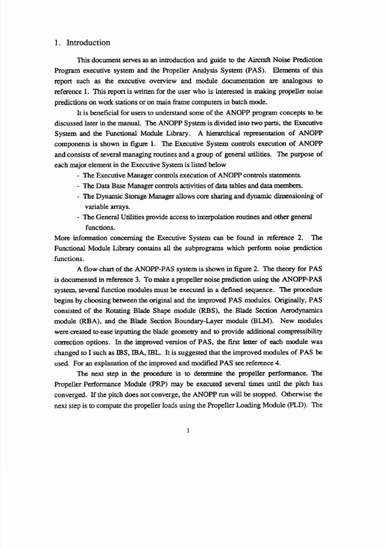
1.
Introduction
This document serves as an introduction and guide to the Aircraft Noise Prediction
Program executive system and the Propeller Analysis System (PAS). Elements of this
report such as the executive overview and module documentation are analogous to
reference 1. This report is written for the user who is interested in making propeller noise
predictions on work stations or on main frame computers in batch mode.
It is beneficial for users to understand some of the ANOPP program concepts to be
discussed later in the manual. The ANOPP
System
is divided into two parts, the
Executive
System and the Functional Module
Library.
A hierarchical representation
of
ANOPP
components is shown in figure 1. The Executive System controls execution of ANOPP
and consists of several managing routines and a group of general utilities. The purpose of
each major element in the Executive System is listed below
- The Executive Manager controls execution of ANOPP controls statements.
- The Data Base Manager controls activities of data tables and data members.
- The Dynamic Storage Manager allows core sharing and dynamic dimensioning of
variable arrays.
The General Utilities provide access to interpolation routines and other general
functions.
More information concerning the Executive System can be found in reference 2. The
Functional Module Library contains all the subprograms which perform noise prediction
functions.
A flow chart of the
ANOPP-PAS
system is shown in figure 2. The theory for PAS
is documented in reference 3. To make a propeller noise prediction using the ANOPP-PAS
system, several function modules must be executed in a defined sequence. The procedure
begins by choosing between the original and the improved PAS modules. Originally, PAS
consisted of the Rotating Blade Shape module (RBS), the Blade Section Aerodynamics
module (RBA), and the Blade Section Boundary-Layer module (BLM). New modules
were created to ease inputting the blade geometry and to provide additional compressibility
correction options. In the improved version of PAS, the first letter of each module was
changed to I such as IBS, IBA, IBL. It is suggested that the improved modules of PAS be
used. For an explanation of the improved and modified PAS see reference 4.
The next step in the procedure is to determine the propeller performance. The
Propeller Performance Module (PRP) may be executed several times until the pitch has
converged. If the pitch does not converge, the ANOPP run will be stopped. Otherwise the
next step is to compute the propener loads using the Propeller Loading Module (PLD). The

8/10/2019 NASA ANOP Propellers
http://slidepdf.com/reader/full/nasa-anop-propellers 8/104
last step is to calculate the propeller noise using the three noise prediction modules which
are the Subsonic Propeller Noise (SPN), the Transonic Propeller Noise (TPN), and the
Propeller Trailing Edge Noise (PTE) Modules.
PAS allows predictions
to be made in several reference frames. For wind tunnel
noise predictions, modules one to six are executed. For flyover noise predictions, modules
one to fourteen are executed. The Atmospheric Module (ATM) and the Atmospheric
Absorption Module (ABS) build the atmospheric table. The flight path is defined by the
Steady Flyover Module (SFO). The Geometry Module (GEO) computes the range and
directivity angles from observer to the noise source. The Tone Propagation module (PRT)
propagates the tone noise from the tone noise modules SPN and TPN and the Broadband
Propagation module (PRO) propagates the broadband noise from the PTE module. The
Noise Level Module (LEV) sums the noise, computes overall sound pressure level
(OASPL), A-weighted sound pressure level, D-weighted sound pressure level, perceived
noise level (PNL), and tone-corrected perceived noise level (PNLT). Effective Noise
Module (EFF) computes effective perceived noise level (EPNL) and sound exposure level
(SEL). A summary of the ANOPP PAS functional modules can be found in Appendix A.
Section 2 contains information resources that can be of aid to users. Module
documentation with
examples containing
informative comments
are
the
subject of
Section
3. Section 4 describes the eleven most often used ANOPP control statements which will
enable the user to set up and execute any ANOPP module. Three examples are provided in
Section 5 which show how to set up a PAS prediction. Section 6 provides a summary of
the improved and updated PAS (third version) which incorporates angle-of-attack in
the
noise prediction.
A
brief description of the capabilities
and
options of PAS is presented in
Section 7. Section 8 contains ten templates to assist users in building a blade geometry
table, an aerodynamics table such as lift and drag, and to compute the performance and the
loads. Templates for the wind tunnel noise prediction and for the flyover noise prediction
are included. Several templates
are
provided as examples to help users build a job for
particular purposes. Results of the studies using PAS and the comparison of the measured
data with
PAS
predictions
are
shown in
Section 9.
The appendices provide supplemental information which will be useful as reference
material. Appendix A is a summary of the functional modules provided in tabular format.
Included in this table is the full title for each module, the associated ANOPP abbreviation,
and a brief description of the function of that module. Appendix B includes a more in-
depth discussion of the TABLE control statement.

8/10/2019 NASA ANOP Propellers
http://slidepdf.com/reader/full/nasa-anop-propellers 9/104
2. Information Resources
Fivemanualsareavailablefor usersto obtainmoreinformationabout PAS. The first
document is the Aircraft Noise Prediction Program User's Manual (ref. 5) which contains a
detailed explanation of the ANOPP executive system. The second document is the
Aircraft
Noise Prediction Program Theoretical Manual, Part 1 which contains the propagation and
atmospheric absorption models (ref. 6). The third document is Part 3 of the
Aircraft
Noise
Prediction Program Theoretical Manual which contains the propeller analysis theories,
reference 3. The fourth document is the NASA Aircraft Noise Prediction Program
Improved Propeller Analysis System (ref. 4). This manual describes the modifications and
improvements that were made to the propeller analysis system. For the user who is
interested in making propeller noise predictions without angle-of-attack on an IBM-PC, the
Aircraft Noise Prediction Program Propeller Analysis System IBM-PC Version User's
Manual (ref. 7) is available.
3

8/10/2019 NASA ANOP Propellers
http://slidepdf.com/reader/full/nasa-anop-propellers 10/104
3. Module Documentation
User
documentation
is maintained
as a
preface to the FORTRAN source code. This
is done to ensure that the correct documentation is available for each version of the program
in existence. This
documentation
is maintained
on
line and is
accessible to
the
user.
Figure 3 shows the format for the documentation of each module. The most
important descriptors to the user
are
the INPUT, OUTPUT, and DATA BASE
STRUCTURE. Under INPUT and OUTPUT, there are user parameters and unit
members. A user parameter retains its value for each execution of a module.
A
unit
member is closely related to a
file
and contains a block of data. Unit members will be
discussed in more detail in section 4.2. The DATA BASE Smactures descriptor provides
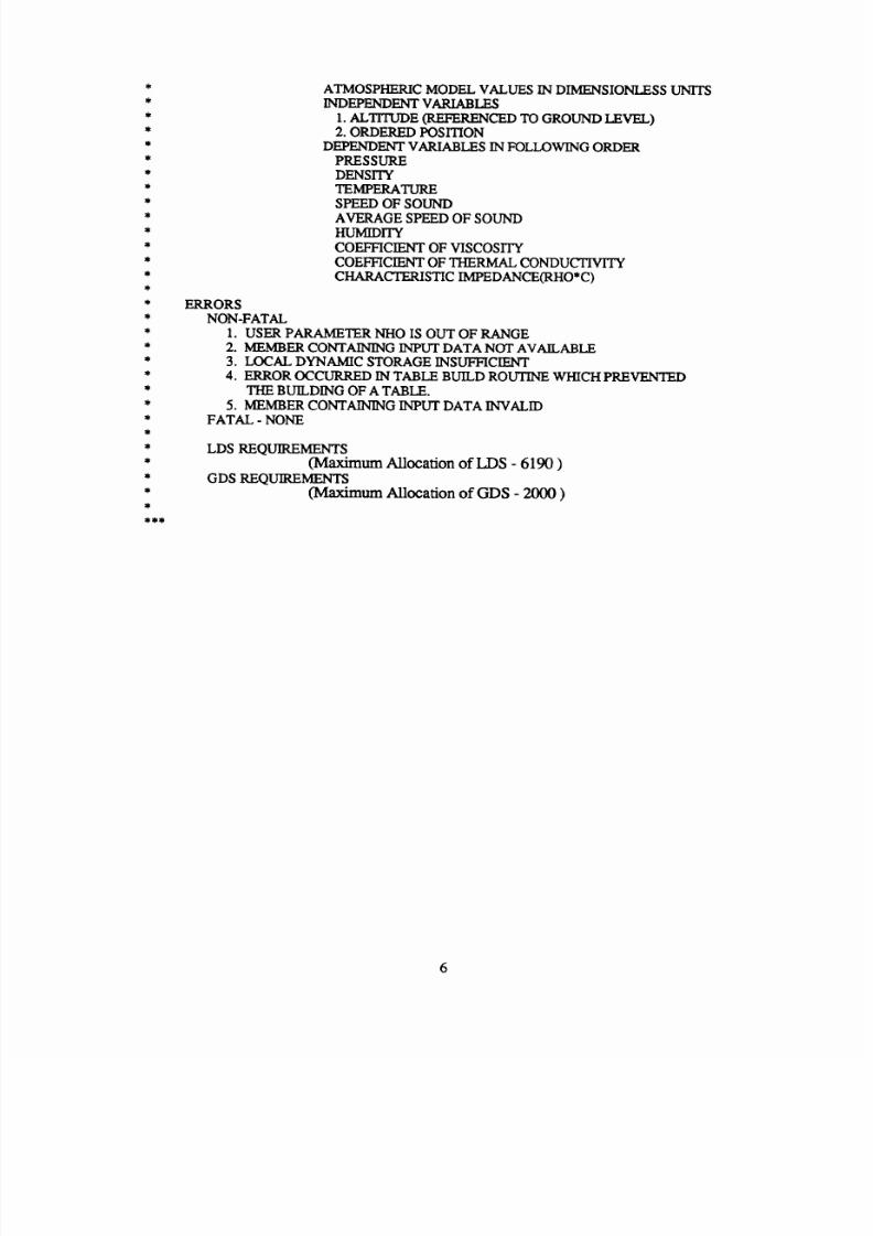
details concerning all unit members. The ERRORS descriptor provides useful error
diagnostics. Computer core requirement are under LDS _ Dynamic Storage) and GDS
(Global Dynamic Storage).
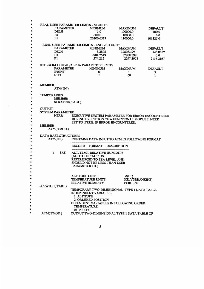
Example 3.1 depicts user documentation for the Atmospheric Module (ATM).
Included in the documentation are various types of user parameters: integer (1), real single
(RS), and alphanumeric (A). Two examples of table members are included. Example 3.1
will be referred to extensively in Section 4 with further examples demonstrating how to use
the documentation.
Example 3.1 Atmospheric Module Prologue
PURPOSE
- BUILD
TABLE
OF ATMOSPHERIC MODEL
DATA
AS
FUNCTIONS
OF
ALTITUDE
AUTHOR
-
SWP(L03KI0/00)
INPUT
USER PARAMETERS
DELH
H1
IUNITS
NHO
P1
IPRINT
ALTITUDE
INCREMENT FOR OUTPUT, M (FT)
GROUND LEVEL ALTITUDE REFERENCED
TO
SEA LEVEL
M(FT)
INPUT UNITS
CODE
--2HSI, INPUTS ARE IN SI UNITS
=THENGLISH,
INPUTS ARE IN
ENGLISH
UNITS
NUMBER OF ALTITUDES FOR
OUTPUT
ATMOSPHERIC
FUNCTIONS
ATMOSPHERIC PRESSURE AT GROUND LEVEL
N/M**2 (LBF/FT**2)
PRINT CODE FOR FORTRAN
WRITE
0 NO PRINT DESIRED
1 INPUT PARAMETER PRINT
ONLY
2
OUTPUT
PRINT ONLY
3 BOTH INPUT PARAMETER AND OU'I_UT PRINT
4
8/10/2019 NASA ANOP Propellers
http://slidepdf.com/reader/full/nasa-anop-propellers 11/104
tO
tO
tO
tO
tO
tO
tO
tO
tO
tO
tO
tO
tO
tO
tO
tO
tO
tO
tO
tO
tO
tO
tO
tO
_t
tO
REAL USER PARAMETER LIMITS - SI UNITS
PARAMETER
MINIMUM
MAXIMUM
DEFAULT
DELH
1.0 100000.0 100.0
H1 -300.0 10000.0 0.0
P1 26200.6517 110000.0 101325.0
REAL USER PARAMETER
LIMITS -
ENGLISH UNITS
PARAMETER
MINIMUM MAXIMUM DEFAULT
DELH 3.2808 328083.99 328.0839
H1
-984.2519
32808.399 0.0
P 1 574.212 2297.3978 2116.2167
INTEGER/LOGICAL/ALPHA PARAMETER LIMITS
PARAMETER MINIMUM MAXIMUM DEFAULT
IPRINT
0
3 3
NHO 1 60 1
MEMBER
ATM(_)
TEMPORARIES
MEMBER
SCRATCH( TAB1 )
OUTPUT
SYSTEM PARAMETER
NERR EXECU'HVE SYSTEM PARAMETER
FOR
ERROR ENCO_D
DURING EXECUTION OF A FUNCTIONAL MODULE. NERR
SET TO .TRUE. IF ERROR ENCOUNTERED.
MEMBER
ATM(
TMOD
)
DATA BASE STRUCTURES
ATM( IN ) CONTAINS DATA INPUT TO ATM IN FOLLOWING FORMAT
RECORD
FORMAT
DESCRIPTION
1 3RS
ALT, TEMP, RELATIVE HUMIDITY
(ALTITUDE, "ALT", IS
REFERENCED TO SEA LEVEL AND
SHOULD NOT BE LESS THAN USER
PARAMETER H1.)
SCRATCH( TAB1 )
ATM( TMOD )
ALTITUDE UNITS
TEMPERATURE UNITS
RELATIVE HUMIDITY
M(Fr)
KELVlN(RANKINE)
PERCENT
TEMPORARY TWO-DIMENSIONAL TYPE 1 DATA TABLE
INDEPENDENT VARIABLES
1. ALTITUDE
2. ORDERED POSITION
DEPENDENT
VARIABLES IN FOLLOWING ORDER
TEMPERATURE
HUMIDITY
OUTPUT TWO-DIMENSIONAL TYPE 1 DATA TABLE OF
8/10/2019 NASA ANOP Propellers
http://slidepdf.com/reader/full/nasa-anop-propellers 12/104
ERRORS
ATMOSPHERIC MODEL VALUES IN DIMENSIONLESS
UNITS
INDEPENDENT VARIABLES
1. ALTITUDE (REFERENCED TO GROUND LEVEL)
2. ORDERED POSITION
DEPENDENT VARIABLES IN FOLLOWING ORDER
PRESSURE
DENSITY
TEMPERATURE
SPEED OF SOUND
AVERAGE SPEED OF SOUND
HUMIDITY
COEFFICIENT
OF
VISCOSITY
COEFFICIENT OF THERMAL CONDUCTIVITY
CHARACTERISTIC
IMPEDANCE(RHO*C)
NON-FATAL
1. USER PARAMETER NHO IS OUT OF RANGE
2. MEMBER CONTAINING INPUT DATA NOT AVAILABLE
3.
LOCAL
DYNAMIC
STORAGE
INSUFFICIENT
4. ERROR
OCCURRED
IN TABLE BUILD ROUTINE
WHICH
PREVENTED
THE
BUILDING
OF A
TABLE.
5.
MEMBER CONTAINING
INPUT
DATA
INVALID
FATAL - NONE
LDS REQUIREMENTS
(Maximum Allocation
ofLDS
-
6190
)
GDS REQUIREMENTS
(Maximum Allocation of GDS - 2000 )
6

8/10/2019 NASA ANOP Propellers
http://slidepdf.com/reader/full/nasa-anop-propellers 13/104
4. Control Statements
Described in this section are ten of the most frequently used statements for
preparing a PAS module for execution. A complete description of all the ANOPP control
statements can be found in reference 5.
Each executive control statement has a specific format indicated in the following
subsections. All control statement formats adhere to the following conventions:
* Each control statement directive is a free-form sequence, using columns 1 to
80
* A control statement may begin in any column and continue across as many as 5
lines to complete the directive.
* Each control statement is terminated by the $ character.
* Comments may appear in columns following the $ character terminator.
* Comments may continue across lines only if the first character on the line is the
$ character terminator.
The general format of a control statement (CS) is as follows:
CSNAME OPERANDS $ COMMENTS
CSNAME control statement name
Listed below are the twelve most frequently used
ANOPP control statements:
ANOPP
STARTCS
LOAD UNLOAD
PARAM
EVALUATE
EXECUTE
ENDCS
UPDATE TABLE
OPERANDS These are the operand fields that are required for each
of the individual control statements.
COMMENTS Any user desired comment can be included.
ANOPP control statements can be divided into two categories, Single Directive and
Multiple Directive. As the name implies, single directive control statements require only
one statement to execute a given function. These commands are described in Section 4.1.
Multiple directive control statements, described in Section 4.2, require sub-commands to
execute a given function.

8/10/2019 NASA ANOP Propellers
http://slidepdf.com/reader/full/nasa-anop-propellers 14/104
4.1
4.1.1
Single Directive Control
ANOPP Pu _rpose:
Fo_at:
Statements
The ANOPP control statement is the first CS in the
input deck.
ANOPP
JECHO=.TRUE. JLOG=.TRUE. $
JECHO: print control during edit phase
/LOG:
print control during execution phase
A complete
list of system parameters
has
been
tabulated on page 3-8 of the ANOPP User's Manual
reference 5.
4.1.2 STARTCS Purpose:
Format:
The
STARTCS
control
statement is
the second
CS
in
the input deck. STARTCS begins the execution.
STARTCS $
4.1.3 LOAD Purpose:
The LOAD control statement loads unit members
from an ANOPP library which has been previously
stored on an external file via the UNLOAD control
statement.
Fo_t-
Example:
4.1.4 UNLOAD Puroose:
LOAD/external fileAmitl ..... unim $
Load the unit ATM from the external file LIBRARY.
Unit ATM contains tables which are required by the
PRT module.
LOAD/LIBRARY/ATM $
The UNLOAD control statement establishes an
ANOPP library for storage of one or more units on
an external file.
Format:
Example:
4.1.5 PARAM Purpose:
Format:
UNLOAD/external file/unit1 ..... unim $
Create an ANOPP library with units UN1 and UN2
and store it on external file EXTFIL.
UNLOAD/EXTFK,/UN 1,UN2 $
The PARAM control statement establishes values of
one or more user parameters.
PARAM pnamel=value 1..... pnamen=value n $

8/10/2019 NASA ANOP Propellers
http://slidepdf.com/reader/full/nasa-anop-propellers 15/104
4.1.6 EVALUATE
Example:
Purpose:
_o_at"
Ex_mpl¢:
pname:
value:
user parameter name
any required integer, real single
precision, logical, or alphanumeric value
Referring to example 3.1, assign values to the
following user parameters:
DELH altitude increment for
output
150.
m
H1 ground level altitude 10. m
NHO number of altitudes for
output atmospheric
functions 50
IPRINT print option output only
IUNITS units metric
PARAM
DELH=150.,H1=10.,NHO=50,
IPRINT=2,IUNITS=2HSI $
The EVALUATE control statement establishes the
value of a user parameter via an arithmetic
expression.
EVALUATE Pnam_xpmssion $
Vname-
expression:
user parameter name
a sequence of constants, user
parameters and functions separated by
operators and parentheses
The arithmetic operators are as
follows:
+ addition
- subtraction
* multiplication
/ division
** exponentiation
It is important to note that the arithmetic operators '+'
and '-' must be preceded and followed by at least one
blank space when used in the EVALUATE
statement.
Additional functions are available as shown in Table 1.
Evaluate the nondimensional velocity V given a
velocity of 102 meters per second and the default
speed of sound, C, equals 340.294 meters per
second.
EVALUATE V=102./C $

8/10/2019 NASA ANOP Propellers
http://slidepdf.com/reader/full/nasa-anop-propellers 16/104
Nanle
ABS
ANTtt.OG
COS
INT
LOG
REAL
SIN
Definition
txl
10 x
cos(x)
convert to
integer
logl0(x), x>0
convert to real
sin(x)
Number of
Ar_rnents
Type of
Aq_ments
any type
I,RS,RD
any type
any type
I,RS,RD
any type
any type
Example
Y = ABS(X)
y_
ANTILOG(K)
Y = COS(X)
X in degrees
Y = INT(X)
Y
=
LOG(X)
Y = REAL(X)
SQRT "(-x, x > 0 1 any type
TAN sin(x)/cos(x) 1 any type Y = TAN(X)
X in degrees
Y
=
SIN(X)
X indegrees
Y = SQRT(X)
Table 1.
Generic
Functions
for
the EVALUATE Control
Statement
4.1.7 EXECUTE Purpose:
Fo_at:
Example:
The EXECUTE control statement calls a specific
functional module
into
execution.
EXECUTE functional
module
name $
Execute the Geometry module, GEO.
EXECUTE GEO $
4.1.8 ENDCS Purpose:
Fo_at:
The ENDCS control statement is the last line in the
input deck and terminates the ANOPP run.
ENDCS $
10
8/10/2019 NASA ANOP Propellers
http://slidepdf.com/reader/full/nasa-anop-propellers 17/104
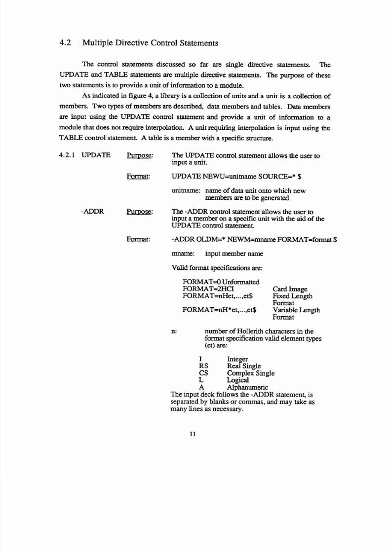
4.2 Multiple Directive Control Statements
The
control
statements discussed
so far
are single directive
statements.
The
UPDATE and
TABLE
statements are multiple directive statements. The purpose of these
two statements is to provide a unit of information to a module.
As indicated in figure 4, a library is a collection of units and a unit is a collection of
members. Two types of members are described, data members and tables. Data members
are input using the UPDATE control statement and provide a unit of information to a
module that does not require interpolation. A unit requiring interpolation is input using the
TABLE control statement. A table is a member with a specific structure.
4.2.1 UPDATE Purpose: The UPDATE control statement allows the user to
input a unit.
Format:
UPDATE
NEWU=unitname SOURCE=* $
unitname: name of data unit onto which new
members are to be generated
-ADDR Purpose:
The -ADDR control statement allows the user to
input a member on a specific unit with the aid of the
UPDATE control statement.
Format:
-ADDR OLDM=* NEWM=mname FORMAT=format $
mname: input member name
Valid format specifications are:
FORMAT=0
Unformatted
FORMAT=2HCI
FORMAT=nHet,
. ... et$
FORMAT=nH*et
..... et$
Card Image
Fixed Length
Format
Variable Length
Format
n_
number of Hollerith characters in the
format specification valid element types
(et) are:
I Integer
RS
Real
Single
CS Complex Single
L Logicra
A Alphanumeric
The input deck follows the -ADDR statement, is
separated by blanks or commas, and may take as
many lines as necessary.
11

8/10/2019 NASA ANOP Propellers
http://slidepdf.com/reader/full/nasa-anop-propellers 18/104
END*
Purpose:
Example:
Examole:
Example:
The END* control statement signals the termination
of input to the unit. This statement is also used with
the TABLE and DATA statements.
A user is required to
input
unit member
OBSERV(COORD) with each record having three
real single
precision
values.
UPDATE NEWU=OBSERV SOURCE=* $
-ADDR OLDM=* NEWM=COORD FORMAT=4H3RS$
i0. 20. 30. $
20. 2O. 2O. $
30. 20. I0. $
END* $
A
user
is required to input unit
SFIEI.D
which
consists of members FREQ, THETA, and PHI.
This unit member
represents
the 1/3-octave band
frequencies, polar directivity angles, and azimuthal
directivity angles required by
every
source noise
module for calculation purposes.
UPDATE NEWU=SFIELD SOURCE=* $
-ADDR OLDM=* NEWM=FREQ FORMAT=4H*RS$
50. 63. 80. 100. 125.
160. 200. 250. 315. 400.
500. 630. 800. i000. 1250.
1600. 2000. 2500. 3150. 4000.
5000. 6300. 8000. i0000. $
ADDR OLDM=* NEWM=THETA FORMAT=4H*RS$
I0. 30. 50. 70. 90. II0.
150. 170. $
-ADDR OLDM=* NEWM=PHI FORMAT=4H*RS$ $
0. $
END* $
A user is required to input unit ATM which consists
of the member IN. This unit member is required as
input to the
Atmosphere
Module. It consists of a
temperature and humidity profile as a function of
altitude.
UPDATE NEWU=ATM SOURCE=* $
-ADDR OLDM=* NEWM=IN FORMAT=4H3RS$
0. 313.2 70. $
i000. 306.7 70. $
2000. 300.2 70. $
3000. 293.7 70. $
4000. 287.2 70. $
5000. 280.7 70. $
END* $
$
12

8/10/2019 NASA ANOP Propellers
http://slidepdf.com/reader/full/nasa-anop-propellers 19/104
4.2.2 TABLE**
Purpose:
Format:
Example 1:
The TABLE control statement builds a table member
in accordance with a set of user supplied instructions
for interpolation.
Type 1 Tables (only type currently available).
TABLE UNIT(MEMBER) 1 SOURCE--* $
INT=0,1,2
IND I=RS,n 1,2,2, independent variable values
separated by commas or blanks
IND2=RS,n2,2,2, independent variable values
separated by commas or blanks
IND3=RS,n3,2,2, independent variable values
separated by commas or blanks
IND4=RS,n4,2,2, independent variable values
separated by commas or blanks
DEP=RS, dependent variable values separated by
commas or blanks
END* $
The integer values nl ..... n4 are the number of values
of
the corresponding independent variables. If the
table has less than four dimensions, then fewer
independent variables are needed. If the independent
variable is ordered position, then the RS is replaced
by a 0 and no independent variable values are
needed. Independent and dependent variable values
may
take as many lines as needed.
The
following
two functions, pressure and
temperature, are input as table ATM(SAMPLE) using
ordered position. The tabulated pressure values are
entered first followed by the temperature values.
IND2 is used to indicate ordered position by
replacing RS with 0 and setting n2 equal to 2
indicating the two functions, pressure and
temperature.
Mfimde pressure mm_tmrature
0. 2116. 510.
2000. 1965. 506.
4000. 1824. 502.
6000. 1692. 498.
TABLE ATM
SAMPLE)
1
INT=0 1 2
INDI=RS 4 2 2 0.
IND2=0 2 2 2
DEP=RS 2116. 1965.
510. 506.
SOURCE=* $
2000. 4000.
6000.
1824.1692.
502. 498.
** See Appendix B of this manual for a detailed discussion of the TABLE control statement
13

8/10/2019 NASA ANOP Propellers
http://slidepdf.com/reader/full/nasa-anop-propellers 20/104
Example 2:
END* $
The following example is a table of the pressure and
the skin friction loadings as functions of the
spanwise station (XI1), the chordwise station (XI2),
and the in-plane station (PSI). This table is built by
PLD or it can be built by the user if the loading
information is available. In this table, beside the
three independent variables
XI1,
XI2, and PSI, there
are two ordered positions: the first one is the
pressure loading and the second one is the skin
friction loading.
XI1 XI2
0.7000 0.0000
0.8000 1.2566
0.8500 1.8850
0.9000 2.5133
0.9500 3.1416
0.9750 3.7699
0.9970 4.3982
5.0265
5.6549
6.2832
PSI
0.000
The first 70 numbers arc the pressure loadings, and
the next 70 numbers are the skin friction loadings.
The table is formed as follows:
TABLE PLD (LOADS ) 1 SOURCE=*
INT= 0 1 2
INDI= RS 7 2 2
0.7000 0.8000 0.8500 0.9000
0.9500 0.9750 0.9970
IND2= RS i0 2 2
0.0000 1.2566 1.8850 2.5133
3.1416 3.7699 4.3982
5.0265 5.6549 6.2832
IND3= RS 1 1 1
0.0000
IND4= 0 2
DEP= RS
0.0649 0.0718
0.0114 0.0126
-0.1681 -0.1873
-0.2728 -0.3350
-0.0724 -0.1310
-0.2257 -0.8863
0.2360 0.2774
0.0501 0.0775
0.1717 0.1965
0 0
0.0907 0.1129 0.1279
-0.1025 -0.1491 0.1600
-0.4114 -0.4462 -0.2604
-0.4054 -0.4530 -0.0585
-0.2345 -0.2339 -0.2190
-1.0035 0.1932 0.2041
0.3473 0.3634 0.4279
0.0873 0.0948 0.0905
0.0542 0.0726 0.0842
14

8/10/2019 NASA ANOP Propellers
http://slidepdf.com/reader/full/nasa-anop-propellers 21/104
0.0959
0.0441
0.0462
0.0906
0.I000
0.0009
0.0017
0.0015
0.0014
0.0028
0.0025
0.0000
0.0014
0.0027
0.0017
0.0012
O.0025
0.0016
0.0013
END* $
0.1018 0.0654 0.0792 0.0351
0.0517 0.0596 0.0635 0.0385
0.0540 0.0674 0.0745 0.0814
0.0860 0.0933 0.0698 0.0786
0.1251 0.1416 -0.0249 -0.0258
0.0011 0.0013 0.0014 0.0016
0.0023 0.0010 0.0012 0.0014
0.0017 0.0018 0.0025 0.0011
0.0016 0.0017 0.0019 0.0021
0.0014 0.0018 0.0020 0.0023
0.0027 0.0037 0.0000 0.0000
0.0000 0.0000 0.0000 0.0000
0.0018 0.0020 0.0022 0.0025
0.0036 0.0011 0.0014 0.0016
0.0019 0.0021 0.0028 0.0010
0.0014 0.0015 0.0017 0.0018
0.0009 0.0012 0.0013 0.0014
0.0017 0.0023 0.0009 0.0011
0.0014 0.0016 0.0017 0.0023
15

8/10/2019 NASA ANOP Propellers
http://slidepdf.com/reader/full/nasa-anop-propellers 22/104
5. Example Programs
In this section, examples will be given showing how to obtain user documentation
for the ATM module and prepare input for execution. The examples include the control
statements necessary to prepare any module for execution.
Example 5.1
To obtain the user
documentation for
the ATM module, the following ANOPP input
deck can be executed. Appendix A lists the names of modules currently included in PAS-
ANOPP. To obtain user documentation for any one of these modules, replace ATM in the
following example with the name of the desired module.
ANOPP JECHO=. TRUE. $
STARTCS $
LOAD LIBRARY MANUAL $
MEMLIST MANUAL (ATM) FORMAT=2HCI
ENDCS $
The MEMLIST is an ANOPP control statement which allows a user to list the contents of a
unit member. The unit MANUAL contains documentation for all functional modules. The
member ATM contains documentation for the ATM module.
Example 5.2
A
demonstration of
the use
of
the Atmospheric Module
(ATM)
is
presented in this
example. The purpose of this module is to generate tables of atmospheric data that can be
used by other modules for subsequent calculations. One table is generated in this example.
This table provides conditions for a standard sea level atmosphere based on a 70% relative
humidity (i.e. 0.2 percent mole fraction). Refer to the Atmospheric Module prologue,
presented as Example 3.1, for more information concerning the input and output of this
module.
ANOPP JECHO=.TRUE. $
STARTCS $
$
$ create the required input data base members
$
UPDATE NEWU=ATM SOURCE=* $
-ADDR OLDM=* NEWM=IN FORMAT=4H3RS$ $
0. 288.15 70.
200. 286.85 70.
400. 285.55 70.
16

8/10/2019 NASA ANOP Propellers
http://slidepdf.com/reader/full/nasa-anop-propellers 23/104
600. 284.25
800. 282.95
I000. 281.65
END* $
$
$ generate atmospheric properties
$
PARAM DELH=I00. HI=0. NH0=II PI=I01325.
$
EXECUTE ATM $
$
ENDCS $
70. $
70. $
70. $
IPRINT=3 $
Example 5.3
The geometry module (GEO) is executed in this example. For any module to
function properly, it must be supplied with certain tables or units of information. Normally
the data can be generated by one module and then used in subsequent modules. In some
cases, it may be more convenient for the user to provide input data required by a module.
This is accomplished using the UPDATE control statement. For example, when examining
pages 4-5 and 4-6 of the ANOPP User's Manual (ref. 5), it can be seen that the Geometry
Module, GEO, requires the following data base structures: ATM(TMOD), FLI(PATH),
and OBSERV(COORD) as input. The table ATM(TMOD) will be generated using the
Atmospheric Module, ATM. The unit member FLI(PATH) can be generated by the SFO
modules or it can be generated by the user. A detailed description of the unit member
FLI(PATH) is given on page 4-7 of reference 6.
ANOPP JECHO=.TRUE. JLOG= TRUE $
STARTCS $
$
$ demonstration problems for geometry module
$
$ create required input data base members
$
UPDATE NEWU=ATM SOURCE=* $
-ADDR OLDM=* NEWM=IN FORMAT=4H3RS$ $
0. 536.670 50. $
END* $
$
PARAM
200
400
600
800
i000
1500
2000
2500
535.957 50. $
535.244 50. $
534.530 50. $
533.817 50. $
533.104 50. $
532.604 50. $
532.236 50. $
532.082 50. $
DELH=I00.
NH0=26
HI=0. UNITS=7HENGLISH
PI=2116.22 IPRINT=3
17

8/10/2019 NASA ANOP Propellers
http://slidepdf.com/reader/full/nasa-anop-propellers 24/104
EXECUTE ATM $
$
$
UPDATE NEWU=FLI SOURCE=* $
-ADDR OLDM=* NEWM=PATH FORMAT=5HIORS$ $
0.0 0. 50. -1000. 0.
20.0 700. 50. -1000. 0.
40.0 1400. 50. -1000. 0.
60.0 2100. 50. -I000. 0.
80.0 2800. 50. -1000. 0.
END* $
$
UPDATE NEWU=OBSERV SOURCE=* $
-ADDR OLDM=* NEWM=COORD FORMAT=4H3RS$ $
END* $
$
I00
I00
i000
i000
2000
2000
50 5
0 I0
-50 5
0 I0
I00 5
-I00 i0
$
$
PARAM CTK=I. 0
$
EXECUTE GEO $
$
$
ENDCS $
level flight path and START=I0 and STOP=50
START=I0. STOP=50. $
0. 0. 0. 0. 0. $
0. 0. 0. 0. 0. $
0. 0. 0. 0. 0. $
0. 0. 0. 0. 0. $
0. 0. 0. 0. 0. $
18

8/10/2019 NASA ANOP Propellers
http://slidepdf.com/reader/full/nasa-anop-propellers 25/104
6. Module Update
6.1 Propeller Performance (PRP) Module Modification
An error was found in equation (36) of the
Aircraft
Noise Prediction Program
Theoretical Manual, Propeller Aerodynamics and Noise (ref. 3), page 10.5-9. This
equation computes the resultant velocity of the fluid in the disk plane in the direction of
rotation. Originally the equation was
V_g (r,_) = -[ (r + _ sin 0iv cos _g) (1 - a2) ]
The
correct equation
becomes
V¥ (r,_g) = -[ (r + k sin otr, sin _) (1 - a2) ]
where
r
X
_p
/g
a2
R
spanwise stations, re R
local advance ratio
propeller angle-of-attack, rack
blade rotation angle, rack
induced tangential velocity component, re rR_
blade length
angular velocity of blade, rad/s
Figure 5 shows results from the incorrect equation and the modified equation for
non-zero angle-of-attack. For a zero angle-of-attack simulation no error is involved in the
prediction.
19

8/10/2019 NASA ANOP Propellers
http://slidepdf.com/reader/full/nasa-anop-propellers 26/104
6.2 Subsonic Propeller Noise (SPN) Module Modification
ThePASmoduleshavebeencontinuously
updated
and validated by comparing with
measured data. A major modification was made for inclusion of shaft angle-of-attack in the
Subsonic PropeUer Noise (SPN) module.
NOIVIENCLATUR_
co ambient speed of sound
f function defining blade surface
local force per unit area of blade acting on fluid
£r component of loading vector in direction of of radiation vector, (2, = £i_i )
M some Mach number
M r component of source Mach vector in direction of radiation vector, ( M r = Mi/'i)
n blade surface normal vector
p' acoustic pressure
PL acoustic pressure produced by loading
Pr acoustic pressure produced by thickness
r distance from source point at emission time to observer
unit vector in direction r
S surface area
t time at which noise signal is received by observer
v
source velocity
vector
V F forward
velocity
of
aircraft
v n source velocity component in direction of blade normal, ( Vn--Vin i )
x
observer
position
in ground fixed frame
y source position in ground fixed frame
ot aircraft angle-of-attack
1"1 source position in blade fixed frame
x time at which noise signal is emitted at source position
Xl/ angle between X1 and rll axes, (xg=_z)
f2 angular velocity of blade
20

8/10/2019 NASA ANOP Propellers
http://slidepdf.com/reader/full/nasa-anop-propellers 27/104
SPN Noise Model
Originally, the PAS ANOPP noise module SPN did not include propeller angle-of-
attack (inflow angle) in the module formulation. Modifications were made to SPN to
incorporate the effects due to angle-of-attack and the new version was tested and compared
with DNW data. In the following discussion, the analysis pertains to the Full Blade
Formulation. The physical model on which the module is based expresses the acoustic
pressure as (ref. 3).
4_p__(x,t) = co,] kr(l_M,l -..as+ Jkr (l_M,) dS
f=0 f=O
+--1 fV£r(rlV[i_'l'c°Mr-c°M2) 1 dS
Co./L
r2(1-- Mr) 3 j,
f=O
(6.1 a)
where
f
_pr(x,t ) =
f=O
-PoVn (r_tIiri + CoM, -CoM2)]
_-S'7._- ,3" ./dS
r (1- M,) j,
P P
p'(x,t) = PL(X,t) + pT(X,t)
(6.1b)
(6.1c)
Since the integrands depend on vector operations, appropriate reference frames must be
established. Three reference frames, which are illustrated in figure 6, are employed in the
computational scheme. These frames are the ground (medium) fixed x-frame, the aircraft
fixed X-frame and the blade fixed r I -frame. At the initial time, the propeller hub is located
at the origin of the x-frame. The x 3 axis defines the flight direction. Initially, the X-frame
coincides with the x-frame but afterwards translate at the constant rate V F, the aircraft
forward velocity. Operations involving blade normals or surface pressures are more easily
computed in the 11 -frame. But it is more convenient to express the source position, y, in
the x-frame then compute r=x-y and _=r/r in the x-frame and transform the vector
components to the rl -frame. Considering equation (6.1), it is seen that the quantities that
need to be revised to include angle-of-attack are
r,
[, v n and M. Note that v n and M are
21
8/10/2019 NASA ANOP Propellers
http://slidepdf.com/reader/full/nasa-anop-propellers 28/104
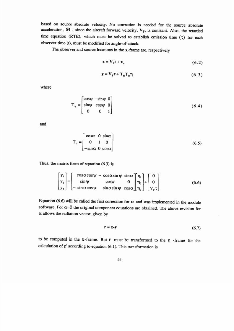
based on source absolute velocity. No correction is needed
for
the source absolute
acceleration, 1_I , since the aircraft forward velocity, VF, is constant. Also, the retarded
time equation (RTE), which must be solved to establish emission time (x) for each
observer time (t), must be modified for angle-of-attack.
The observer and source locations in the x-frame are, respectively
x=VFt+x ° (6.2)
y = VF'C+ T_T_ri
(6.3)
where
T.-lsi7
os 0
(6.4)
and
T0t _
cosa0 01 siva ]
-sina 0 cosaj
(6.5)
Thus, the matrix
form
of equation (6.3) is
Iyllcos cos
2 = sin_g
Y3 - sin
acos_g
-cosasin_
sinai[tit
] I 0 ]
cos
sinasinxg cosaJ[_rl3J LvFxJ
(6.6)
Equation (6.6) will be called the fhst correction for
a
and was implemented in the module
software. For
a---O
the original component equations are obtained. The above revision for
a allows the radiation vector, given by
r = x-y (6.7)
to be computed in the
x-frame. But
r must be transformed to the rl
-frame
for the
calculation of p' according to equation (6.1). This transformation is
22

8/10/2019 NASA ANOP Propellers
http://slidepdf.com/reader/full/nasa-anop-propellers 29/104
El] Frl
2 = T_IT_ ' r 2
r3 _ r3
x
(6.8)
where
cosvcosa
sin
V - cosvsinot-
-
sinvcoso_
cos V
sinvsina
sin a 0 cos o_
(6.9)
Equation (6.8) represents the
second
correction for a in the
SPN
module. The absolute
velocity for each source point is expressed as
V=VF+f2 x rl (6.10)
In the 11-frame, equation (6.10) can be written as
r°l
=T_IT_ 1
0
+f_xT
LVFJ
(6.11)
From equation (6.11), k is found that the components ofv are
Evl]vFin c°s l
2 =
:_rl:
V F sin ot sin Xl
v 3 V F coso_
(6.12)
This is the third correction for ct. As indicated in equation (6.1), emission times must be
found for the RTE:
Ix(t)
_
y(x)[2
= c.2(t
_ ,1:)2
(6.13)
Using equations (6.2) and (6.3) allows the above relation to be stated in terms of 1]
-frame
components as
23

8/10/2019 NASA ANOP Propellers
http://slidepdf.com/reader/full/nasa-anop-propellers 30/104
['Fv_T_l[XoVr(t-'_)]-B[ 2 = c2(t- _) 2 (6.14)
where
'Fv_'F_
[Xo
+
VF(t-
x)]
= T_,_T_='
Lx3
xl]
2
+ VF(t -
x)
(6.15)
Equation (6.14) produces the following retarded time relation
A¢ 2 + B¢ +C + cos(O+D) + EOcos(¢+F) = 0
(6.16)
where
¢ = _('_-t )
2
A= Co-
2Tlx*_ 2
B = vF[-x;sina + (x; - rl3)cosa]
_2TIX"
C = Ix'2 + r12+ (x; + 11)_]
2x'T1
D = W,_-Wx+f_t
V F sin
a
E =
f2x °
F =
-V',I
+f2t
x_ = x lCosa- x 3sina
x; = x 3cosa+ xlsina
* 4 * 2 2
= X 1 + X 2
24
8/10/2019 NASA ANOP Propellers
http://slidepdf.com/reader/full/nasa-anop-propellers 31/104
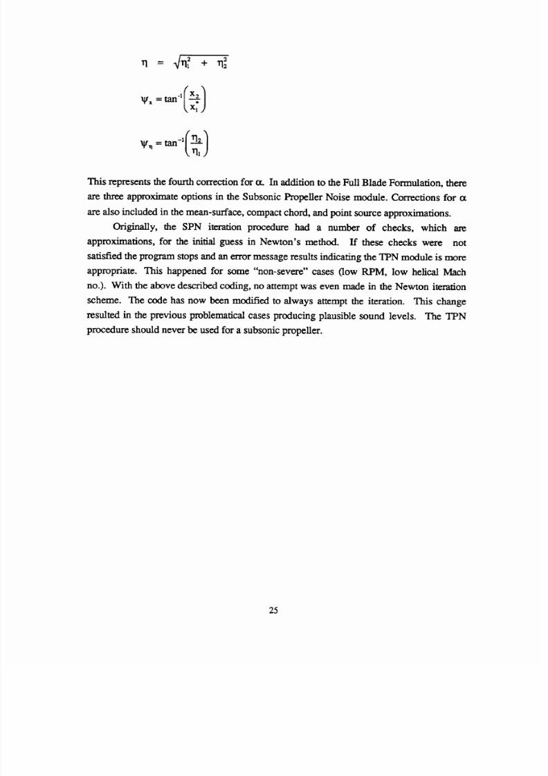
n
- +
This represents
the fourth correction
for o_. In addition to
the
Full
Blade Formulation,
there
are three approximate options in the Subsonic PropeUer Noise module. Corrections for ot
are also included in the mean-surface, compact chord, and point source approximations.
Originally, the SPN iteration procedure had a number of checks, which are
approximations, for the initial guess in Newton's method. If these checks were not
satisfied the program
stops
and an error message results indicating the TPN
module
is
more
appropriate. This happened for some "non-severe" cases flow RPM, low helical Mach
no.). With the above described coding, no attempt was even made in the Newton iteration
scheme. The code has now been modified to always attempt the iteration. This change
resulted in the previous problematical cases producing plausible sound levels. The TPN
procedure should never be used for a subsonic propeller.
25
8/10/2019 NASA ANOP Propellers
http://slidepdf.com/reader/full/nasa-anop-propellers 32/104
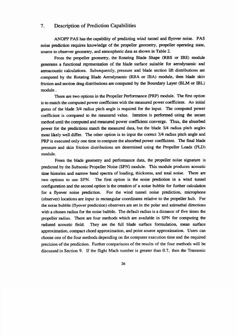
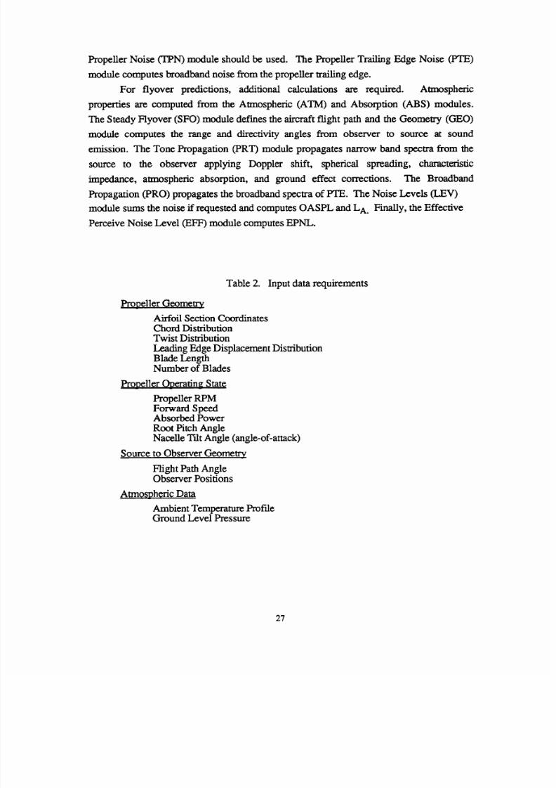
7. Description of Prediction Capabilities
ANOPP PAS has the capability of predicting wind tunnel and flyover noise. PAS
noise prediction requires knowledge of the propeller geometry, propeller operating state,
source to observer geometry, and atmospheric data as shown in Table 2.
From
the
propeller
geometry, the Rotating Blade
Shape
(P,
BS or IBS)
module
generates a functional
representation
of
the blade surface suitable
for
aerodynamic
and
aeroacoustic calculations. Subsequently, pressure and blade section lift distributions are
computed by the Rotating
Blade
Aerodynamic (RBA or IBA) module, then blade skin
friction and section drag distributions are computed by the
Boundary
Layer (BLM or IBL)
module.
There are two options in the Propeller Performance (PRP) module. The first option
is to match the computed power coefficient with the measured power coefficient. An initial
guess of the blade 3/4
radius
pitch angle is
required
for the input. The computed power
coefficient is compared
to the
measured value.
Iteration
is performed using the secant
method until the computed and measured power coefficient converge. Thus, the absorbed
power for the predictions match the measured data, but the blade 3/4 radius pitch angles
most likely well differ. The other option is
to
input the correct
3/4 radius
pitch angle and
PRP
is executed only one time
to
compute the absorbed power coefficient. The final blade
pressure and
skin
friction distributions are determined using
the
Propeller Loads (PLD)
module.
From
the blade geometry and performance data, the propeller noise signature is
predicted by the Subsonic Propeller Noise (SPN) module. This module produces acoustic
time histories and narrow band _ of loading, thickness, and total noise. There are
two options to use SPN. The trn'st option is the noise prediction in a wind tunnel
configuration and the second option is the creation of a noise bubble for further calculation
for a flyover noise prediction. For the wind runnel noise prediction, microphone
(observer) locations are input in rectangular coordinates relative to the propeller hub. For
the noise bubble (flyover prediction) observers are set in the polar and azimuthal directions
with a chosen
radius
for the noise bubble, The default
radius
is a distance of five times
the
propeller radius. There are four methods which are available in SPN for computing the
radiated acoustic field. They are
the
full blade surface formulation, mean surface
approximation, compact chord approximation, and point source approximation. Users can
choose one of the four methods depending on the computer execution time and the required
precision of the prediction. Further comparisons of the results of the four methods will be
discussed in Section 9. If the flight Mach number is greater than 0.7, then the Transonic
26
8/10/2019 NASA ANOP Propellers
http://slidepdf.com/reader/full/nasa-anop-propellers 33/104
Propeller
Noise
(TPN) module should
be used. The
PropcUcr
Trailing
Edge
Noise (PTE)
module computes broadband noise from the propeUer trailing edge.
For flyover predictions, additional calculations are required. Atmospheric
properties are computed from the Atmospheric (ATM) and Absorption (ABS) modules.
The Steady Hyover (SFO) module def'mes the aircraft flight path and the Geometry (GEO)
module computes
the range and
dircctivity angles from observer
to
source at sound
emission. The Tone Propagation (PRT) module propagates narrow band spectra from the
source
to the
observer
applying
Doppler shift, spherical spreading, characteristic
impedance, atmospheric absorption,
and ground
effect corrections.
The
Broadband
Propagation
(PRO)
propagates
the
broadband spectra of PTE.
The Noise
Levels
(LEV)
module sums the noise if requested and computes OASPL and LA. Finally, the Effective
Perceive
Noise Level (EFF)
module computes EPNL.
Table
2. Input
data
requirements
Propeller Geometry
Airfoil Section
Coordinates
Chord
Distribution
Twist Distribution
Leading Edge Displacement Distribution
Blade Length
Number of Blades
Propeller _Operating State
Propeller RPM
Forward Speed
Absorbed Power
Root Pitch Angle
Nacelle Tilt Angle (angle-of-attack)
Source to Observer Geometry
Hight
Path Angle
Observer Positions
Atmo_hedc Data
Ambient
Temperature Profile
Ground Level Pressure
27
8/10/2019 NASA ANOP Propellers
http://slidepdf.com/reader/full/nasa-anop-propellers 34/104
8. PAS Program Templates
This section contains ten templates which have been developed to demonstrate the
types of problems that can be solved using ANOPP-PAS. Templates one and two
demonstrate how the blade geometry is input using the improved and the original ANOPP-
PAS modules. Templates three and four demonstrate how to compute the propeller
performance. In template three, the blade pitch is known and the performance is computed
directly by the PLD module. In template
four,
the
pitch
is unknown and an
iterative
scheme is used. Template five demonstrates how the propeller loads are calculated using
the PLD module. Template six demonstrates how measured propeller loads can be input
directly,
bypassing
the
PLD module.
Templates seven and
eight
demonstrate how the
propeller noise is calculated using the SPN module. Template seven calculates the near-
field noise. Template eight calculates the noise on a sphere around the propeller (i.e.
"sound bubble") for propagation to the far-field. Finally, template nine demonstrates a
simple flyover prediction and then template ten demonstrates how
ANOPP-PAS
can be
used to add noise from multiple rotors such as the tilt rotor. Each template builds upon the
information of the preceding template. The input and output of each module can be found
in reference 3. In most cases this information is also available on line using the "man"
command on UNIX systems and the HELP command on VMS systems. The ANOPP
control
statements
are described in section 4
of
this
document. Additional
information
concerning the control statements can be found in reference 5.
8.1 Blade Geometry
8.1.1 Template 1 - The Improved Version of PAS
Problem: Given
a
propeller blade geometry with 5 identical cross
sections,
tables
of
cross sectional lift, drag and pressure coefficients are built in the given ranges of angle-of-
attack and Mach number.
Solution: The fast step is to transform the airfoil section data from Cartesian
coordinate to the elliptical coordinate defined by the inverse Joukowski transformation.
This procedure is performed in IBS. The second step is to compute the sectional lift
coefficient using the Kutta-Joukowski theorem. Also, the pressure coefficient is computed
using Bemoulli's equation. The compressibility con'ection is extended to subsonic flow by
Karman-Tsien or Glauert compressibility corrections in IBA. Finally, the profile drag
coefficient is computed by the method of Squire and Young in IBL.
28

8/10/2019 NASA ANOP Propellers
http://slidepdf.com/reader/full/nasa-anop-propellers 35/104
Input thebladegeometryasrequiredn theImprovedBladeShape(IBS) Module. A
descriptionof thebladegeometrycanbe found in reference3. Thebladecrosssectionis
describedin rectangularcoordinates. Chordwiselocationsare designatedby x where
x=0.0 is theleadingedgeandequalsx=l.0 is the trailing edge. The uppersurfacey is
input beforethelower surfacey. Coordinatesx and y arenormalizedby crosssection
chord, c.
In this template, there are 5
propeller
cross sections with the same spatial
coordinates. The improved modules are used to shorten the input and provides additional
compressibility correction options. Beside the Cartesian coordinates of the cross sections,
other informations about the propeller are required. After showing how many cross
sections are given, the next five lines which have eight numbers in each are
- Spanwise station normalized by the blade radius R
- Leading-edge abscissa as shown in the following plot normalized by R
- Leading-edge ordinate as shown in the following plot normalized by R
- Chord length, normalized by R
- Leading-edge radius, re chord length of the cross section
- Blade twist angle measured positive clockwise looking from hub toward
propeller tip
- Number of x,y pairs for the upper surface
- Number of x,y pairs for the lower surface
An illustration of the blade geometry is shown below.
leading edge
ordinate
.,¢"
""r12eading
/
....
edg / y .---
/
_leading edge
..
......... _S
., X
leading edge
abcissa
Til
29

8/10/2019 NASA ANOP Propellers
http://slidepdf.com/reader/full/nasa-anop-propellers 36/104
The
followings
are
considerations that users
should
remember to
avoid
errors
and also
to
obtain better predictions.
- The spanwisc stations (XI1), rc R (blade length) array should be in the range of
XI1 in the given blade geometry.
- The chordwise stations (XI2), re 2_, are from 0.0 to 1.0. From 0.0 to 0.5, these
arc points in chordwise direction from trailing edge to leading edge for upper surface. For
lower surface, XI2 is fzom 0.5 to 1.0 from leading edge to wailing edge. For more
accurate
results,
it
is important to refine the grids
at
the
leading
edge.
- Blade section angles-of-attack and Mach numbers should be input to adequately
cover the range of the flight condition of the prediction.
ANOPP JECHO=. TRUE. JLOG=.FALSE.
STARTCS $
PARAM R -- 13.205 $ blade radius in ft
PARAM IUNITS = 7HENGLISH $ use English units
UPDATE NEWU=GEOM SOURCE=* $
-ADDR OLDM=* NEWM=BLADE
FORMAT=0
$
5 $ five spanwise stations
5 $ five identical airfoil _ections
0.00 -0.0106 0.000 0.043 0.025 0.00 20 19 $ 0%
0.25 -0.0106 -0.000 0.043 0.025 -2.25 20 19 $ 25%
0.50 -0.0106 -0.001 0.043 0.025 -4.50 20 19 $ 50%
0.75 -0.0106 -0.001 0.043 0.025 -6.75 20 19 $ 75%
1.00 -0.0106 -0.002 0.043 0.025 -9.00 20 19 $100%
1.00000
.97000
94000
85000
79000
73000
67000
61000
.55000
.49000
.43000
37000
31000
25000
19000
13000
O7OOO
01750
00250
.00000
.00250
.01000
.04000
.00158
$
.00674
.01172
.02566
.03417
.04207
.04937
.05600
.06191
.06695 $
.07097 $
.07376
$
.07499
.07427 $
.07095 $
.06399 $
.05108 $
.02772
.01090
$
.o00oo $
-.01090 $
-.02130 $
-.04035 $
station
station
station
station
station
3O

8/10/2019 NASA ANOP Propellers
http://slidepdf.com/reader/full/nasa-anop-propellers 37/104
END* $
$
$
I0000
16000
22000
28OO0
34000
40000
46000
.52000
.58000
.64000
.70000
.76000
.82000
.88000
.94000
1.00000
UPDATE NEWU=GRID SOURCE =* $
- 05853 $
- 06802 $
- 07298 $
- 07491 $
- 07459 $
- 07254 $
- 06910 $
- 06454 $
- 05905 $
-.05277 $
-.O458O $
-.03819 $
-.02999 $
-.02117 $
-.01172 $
-.0O158 $
END* $
$
$
-ADDR OLDM=* NEWM=XII FORMAT=4H*RS$ $
0.200 0.400 0.600 0.700 0.750
0.850 0.900 0.925 0.950 0.975
-ADDR OLDM =* NEWM=XI2 FORMAT=4H*RS$ $
0 00
0 20
0 41
0 46
0 51
0 56
0 625
0 85
0.025 0.05 0.i0 0.15
0.25 0.30 0.35 0.40
0 .42 0 .43 0 .44 0 .45
0.47 0.48 0.49 0.50
0.52 0.53 0.54 0.55
0.57 0.58 0.59 0.60
0.65 0.70 0.75 0.80
0.90 0.95 0.975 1.00
$
$
$
$
_DATE NE_=IBA SOURCE =* $
-_DR O_M =* NE_=MACH FORMAT=4H*RS$ $
0.I 0.3 0.5 0.7 $
-_DR OLDM =* NE_=ALPHA FORMAT=4H*RS$ $
-6.0 -3.0 0.0 3.0 6.0 5
END* $
0.800
1.000 $
The values of section Mach number and angle-of-attack in degrees
at which the blade section aerodynamics are computed are given here:
Choose the compressibility correction options
EXECUTE IBS $
PARAM ICL = 1 $ Glauert compressibility correction for the lift
$ coefficient
PARAM ICP = 1 $ Glauert compressibility correction for the pressure
$ coefficient
EXECUTE IBA $
EXECUTE IBL $
31

8/10/2019 NASA ANOP Propellers
http://slidepdf.com/reader/full/nasa-anop-propellers 38/104
UNLOADBLDGEOM IBS, IBA, IBL $
ENDCS $
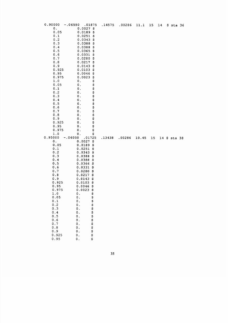
8.1.2 Template 2 - Blade description using the original PAS
modules.
Problem: Given a propeller blade geometry with 8 different cross sections, build
tables of cross sectional lift, drag and pressure coefficients in the given ranges of angle-of-
attack and Math number.
Solution: This template similar to template 1 except it serves as example for the use of
the
original
RBS, RBA and BLM modules. If IBS, IBA and IBL are preferred then in the
blade geometry input, after the "8 $" line, the next added line is 1, 1, 1, 1, 1, 1, 1, 1 $ to
show that there are 8 different cross sections. Note that the leading edge is input
first.
The
same resuks are provided as in template 1 except the unit-members or table names should
start with RBS, RBA or BLM instead of IBS, IBA and IBL.
ANOPP $
$
STARTCS $
$
$
$
$
$
specify 21 evenly
spaced chordwise grid points
UPDATE NEWU=GRID SOURCE=* $
-ADDR OLDM=* NEWM=XI2 FORMAT=4H*RS$ MNR=I $
.00 .05 .10 .15 .20 .25 .30 .35
.40 .45 .50 .55 .60 .65 .70 .75
.80 .85 .90 .95 1.0 $
END* $
PARA/_ R=I.0 IUNITS=2HSI $
CREATE GEOM$
UPDATE NEWU=GEOM SOURCE=* $
-ADDR NEWM=BLADE OLDM =* FORMAT=0 $
8 $ NO. OF RADIAL SECTIONS
0.30000 -.05690 .03090 .14375 .02166 28.5
0. 0.0151 $
0.05 0.0475 $
0.I 0.0632 $
15 14
sta 12
32

8/10/2019 NASA ANOP Propellers
http://slidepdf.com/reader/full/nasa-anop-propellers 39/104
0.2
0.3
0.4
0.5
0.6
0 7
0 8
0 9
0 925
0 95
0 975
1 0
0 O5
0 1
0.2
0.3
0.4
0.5
0.6
0.7
0.8
0.9
0. 925
0.95
0.97
1.0
0.45000
O.
0.05
0.1
0.2
0.3
0.4
0.5
0.6
0.7
0.8
0.9
0. 925
0.95
0.975
1.0
0.05
0.i
0.2
0.3
0.4
0.5
0.6
0.7
0.8
0.9
O. 925
O.95
0.975
1.0
0.60000
O.
0 0846 $
0 0950 $
0 0979 $
0 0950 $
0 0846 $
0 0718 $
0 0544 $
0 0324 $
0 0151 $
0 0116 $
0 0069 $
0 0000 $
-0. 0116 $
-0. 0185 $
-0. 0278 $
-0. 0324 $
-0.0336 $
-0. 0324 $
-0. 0301 $
-0. 0266 $
-0 0220 $
-0 0168 $
-0 0151 $
-0 0116 $
-0 0069 $
0 0000 $
-.06932 .02730
O. 0230 $
0.0466 $
O. O578 $
O. 0702 $
O. O755 $
0.0741 $
0.0689 $
O. 0603 $
O. 0490 $
O. 0364 $
O. 0231 $
O. 0153 $
O. OO82 $
0 0031 $
0 0000 $
0 OO82 $
0 0051 $
0 0021 $
0 $
0 $
0 $
0 $
0 $
0 $
0 $
0 $
0 $
0 $
0 $
-.07300 .02450
O. 0089 $
.16300
.16875
.00919
.00395
21.5
16.9
15 14 $ sta 18
15 14 $ sta 24
33

8/10/2019 NASA ANOP Propellers
http://slidepdf.com/reader/full/nasa-anop-propellers 40/104
0.05
0.i
0.2
0.3
0.4
0.5
0.6
0.7
0.8
0.9
0.925
0.95
0.975
1.0
0.05
0.1
0.2
0.3
0.4
0.5
0.6
0.7
0.8
0.9
0. 925
0.95
0. 975
1.0
O.75000
O.
0.05
0.1
0.2
0.3
0.4
0.5
0.6
0.7
0.8
0.9
0.925
0.95
0.975
1.0
0.05
0.1
0.2
0.3
0.4
0.5
0.6
0.7
0.8
0.9
0.925
0.95
0.975
1.0
O. 0281
$
0 0395 $
0 0513 $
0 0553
$
0 0543 $
0 0513 $
0 0454
$
O. 0375 $
O. 0286 $
0. 0183 $
O. 0148 $
0. 0099 $
O. 0049 $
O. 0000 $
0.0029 $
0.0010 $
O. $
O. $
O. $
O. $
O.
$
O.
$
O.
$
o.
$
O. $
O. $
O. $
O.
$
-.07450 .02050
0.0033 $
O. 0201 $
O. 0281 $
O. 0382 $
0.0422 $
0.0427 $
0.0412 $
O. 0372 $
O. 0312 $
O. 0231 $
O.
0151 $
0.0101 $
o. 0071 $
O. 0O40 $
O. $
O. $
0 $
0 $
0
$
0 $
0 $
0
$
0 $
0 $
0 $
0
$
0 $
0 $
0
$
.16575 .00352 13.5 15 14 $ sta 3O
8/10/2019 NASA ANOP Propellers
http://slidepdf.com/reader/full/nasa-anop-propellers 41/104
0.90000
O.
0.05
0.I
0.2
0.3
0.4
0.5
0.6
0.7
0.8
0.9
0.925
0.95
0.975
1.0
0.05
0.1
0.2
0.3
0.4
0.5
0.6
0.7
0.8
0.9
0.925
0.95
0.975
1.0
0.95000 -.06050
O.
0.05
0.1
0.2
0.3
0.4
0.5
0.6
0.7
0.8
0.9
0.925
0.95
0.975
1.0
0.05
0.i
0.2
0.3
0.4
0.5
0.6
0.7
0.8
0.9
0.925
0.95
-.06550 .01875
O. 0027 $
0.0189 $
0. 0251 $
O. 0343 $
o.0388 $
0 0388 $
0 0365 $
0 0331 $
0 o280 $
0 0217 $
0 0143 $
0 0103 $
0 0046 $
0 0023 $
o $
o $
o $
o. $
o. $
o. $
o. $
o. $
o. $
o. $
o. $
o. $
o. $
o. $
o. $
.01725
O. 0027 $
O. 0189 $
0. 0251 $
0. 0343 $
0.0388 $
0.0388 $
O. 0366 $
O. 0331 $
o.0280 $
O. 0217 $
0. 0143 $
0. 0103 $
O. 0046 $
0. 0023 $
O. $
o $
o $
o $
o $
0 $
o $
o $
o $
o $
o $
o $
0 $
.14575
.13438
.00286
.00286
ii.i
10.45
15 14 $ sta 36
15 14 $ sta 38
35

8/10/2019 NASA ANOP Propellers
http://slidepdf.com/reader/full/nasa-anop-propellers 42/104
0.975
1.0
0.97500
O.
0.05
0.i
0.2
0.3
0.4
0.5
0.6
0.7
0.8
0.9
0.925
0.95
0.975
1.0
0.05
0.1
0.2
0.3
0.4
0.5
0.6
0.7
0 8
0 9
0 925
0 95
0 975
1 0
0.99750
O.
0.05
0.1
0.2
0.3
0.4
0.5
0.6
0.7
0.8
0.9
0.925
0.95
0.975
1.0
0.05
0.1
0.2
0.3
0.4
0.5
0.6
0.7
0.8
0.9
O.
$
O.
-.05250 .01750
O. 0O20
$
0. 0178
0. 0244
0. 0311
0. 0340
O. 0355
0. 0340
0. 0304
0. 0259
0.0200
O. 0133
O. 0074
0.0029
0.0015
0 $
0
0
0
$
0
$
0
$
0 S
0 $
0
$
0 $
0 $
0 $
0 $
0 $
0
-.0125 .00925
O.002
0. 0178
0 0244
0 0311
0 0340
0 0355
$
0 0340
0 0304
0 0259 $
O.
0200
O. 0133
O. 0074
0.0029
$
O. 0015
$
O. $
O. $
O.
O. $
O.
$
O. $
O.
$
O. $
O. $
O.
O. $
.11250
.02950
.00296
.00296
I0.12
9.83 15
15 14 $ sta
39
14 $ sta
39.9
36

8/10/2019 NASA ANOP Propellers
http://slidepdf.com/reader/full/nasa-anop-propellers 43/104
0. 925 0. $
0.95 0. $
0.975 0. $
1.0 0. $
END* $
compute smooth blade shape using RBS module
EXECUTE RBS $
compute blade aerodynamics with RBA & BLM module
EVALUATE R = 40. * .0254 $ convert inches to meters
PARAM VNU = .17894E-04
CA=
340.29 $
EVALUATE RINF = CA * R VNU $
PARAM IPRINT=3 NORDER=4 $
CREATE
REA$
UPDATE NEWU=RBA SOURCE=*
-ADDR NEWM=MACH OLDM = *
.I 3 5 7
-ADDR NEWM=ALPHA OLDM =*
-6. -3. 0.0 3.
END*$
$
FORMAT=4H*RS$ MNR=I$
$
FORMAT=4H*RS$ MNR=I$
6. $
EXECUTE RBA $
EXECUTE BLM $
UPLIST $
save the tables created up to this point on file BCPLIB
UNLOAD BCPLIB RBS,RBA, BLM $
ENDCS $
37
8/10/2019 NASA ANOP Propellers
http://slidepdf.com/reader/full/nasa-anop-propellers 44/104
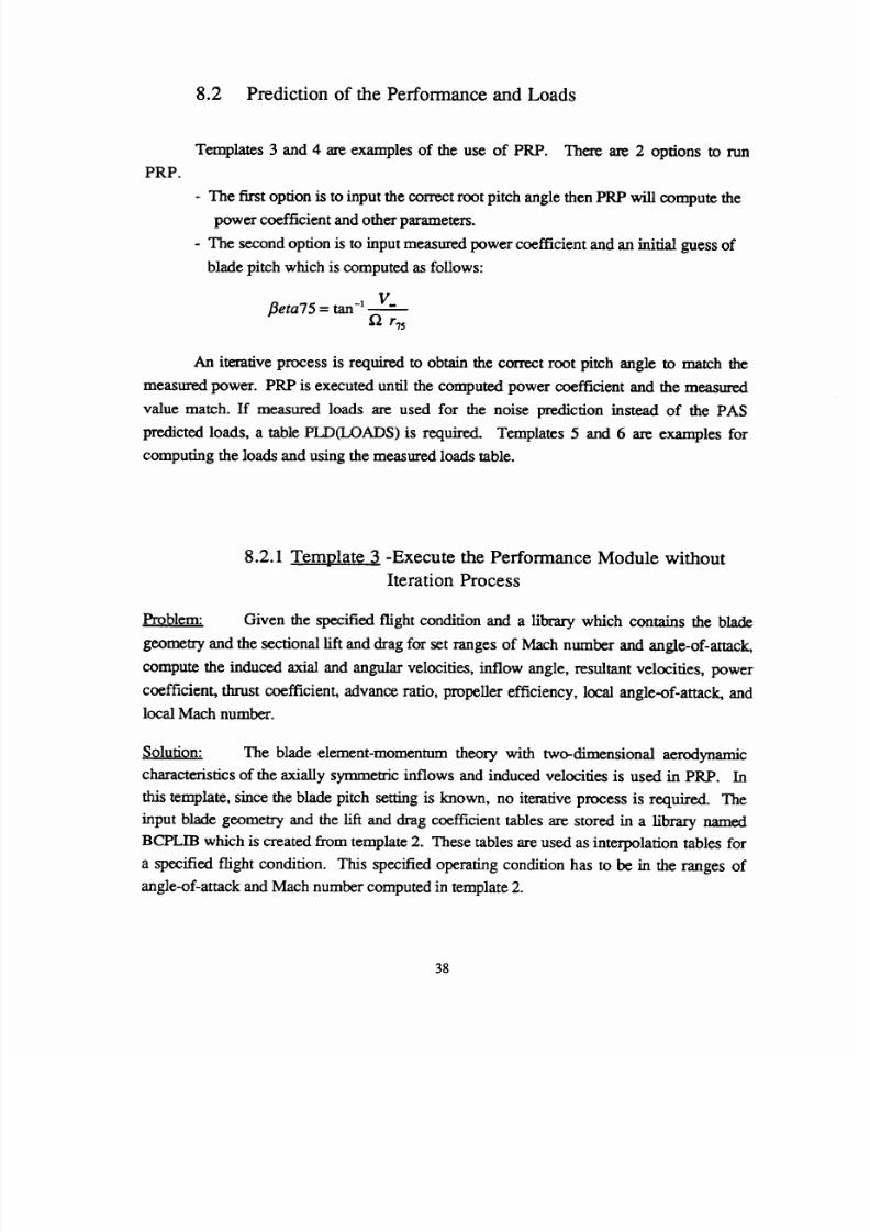
8.2 Prediction of the Performance and Loads
PRP.
Templates 3 and 4 are examples of the use of PRP. There are 2 options to run
- The first option is to input the correct root
pitch
angle then PRP will compute the
power coefficient and other parameters.
- The second option is to input measured power coefficient and an initial guess of
blade pitch which is computed as follows:
fleta75
= tan -1 1t".
f_r75
An iterative process is required to obtain the correct root pitch angle to match the
measured power. PRP is executed until the computed power coefficient and the measured
value match. If measured loads are used for the noise prediction instead of the PAS
predicted loads, a table PLD0.,OADS) is required. Templates 5 and 6 are examples for
computing the loads and using the measured loads table.
8.2.1 Template 3 -Execute the Performance Module without
Iteration Process
Problem: Given the specified flight condition and a library which contains the blade
geometry and the sectional lift and drag for set ranges
of
Mach number and angle-of-attack,
compute the induced axial and angular velocities, inflow angle, resultant velocities, power
coefficient, thrust coefficient, advance ratio, propeller efficiency, local angle-of-attack, and
local Mach number.
Solution: The blade element-momentum theory with two-dimensional aerodynamic
characteristics of the axially symmetric inflows and induced velocities is used in PRP. In
this template, since the blade pitch setting is known, no iterative process is required. The
input blade geometry and the lift and drag coefficient tables are stored in a library named
BCPLIB
which is created from template 2. These tables are used as interpolation tables for
a specified flight condition.
This
specified operating condition has to be in the ranges of
angle-of-attack and Mach number computed in template 2.
38

8/10/2019 NASA ANOP Propellers
http://slidepdf.com/reader/full/nasa-anop-propellers 45/104
ANOPP $
STARTCS $
LOAD BCPLIB RBS RBA BLM $
PARAM ALPHAP = 0.
PARAM IDPDT = 0
PARAM BETA75 = 19.9
PARAM VF = 51.2
PARAM ORIG = 13.5
EVALUATE BETA = BETA75
EVALUATE THETAR = BETA *
EVALUATE ALPHAP = ALPHAP
PARAM MACHRF = 0.69
PARAMMZ = 0.26
EXECUTE PRP $
ENDCS $
$ set propeller angle-of-attack in degrees
$ propeller loading is steady
$ propeller
3/4
span pitch angle in degrees
$ flow velocity in m/s
$ blade twist angle at 3/4 span in degrees
$ (obtain from the blade geometry at 3/4
$ span)
- ORIG
$ compute root pitch in degrees
PI 180.
$ convert root pitch to radians
* PI 180.
$ convert propeller angle-of-attack to
$ radians
$
$
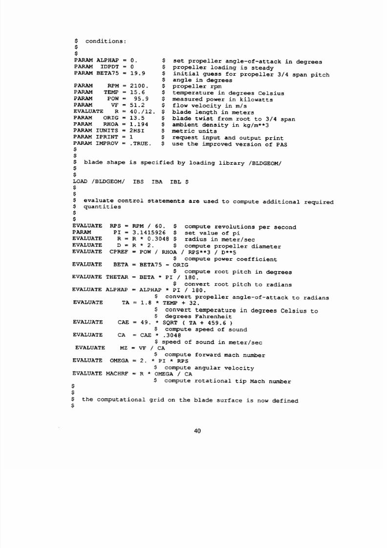
8.2.2 Template 4 - Execute the Performance Module with
Iteration Process
Problem: The power input is known. The blade geometry and the lift and drag
coefficient tables are provided from template 1. Compute the performance and find the
correct root pitch angle in the specified operating condition.
Solution: This template is the same as template 3. The difference is the power input is
known in this problem when the root pitch setting is known in template 3. An iterative
process is required to find the correct root pitch angle. PRP is executed until the computed
power coefficient matches the measured power coefficient.
ANOPP JECHO=.TRUE. JLOG=.FALSE.
STARTCS $
$
$
$
$
$
$
$
LENGL=20000 $
this run predicts the noise for the FAA DNW wind tunnel propeller
tests. It applies a correction to the propeller blade pitch to
match the measured power.
the following parameters set the tunnel and propeller operating
39
8/10/2019 NASA ANOP Propellers
http://slidepdf.com/reader/full/nasa-anop-propellers 46/104
$ conditions:
$
PARAM
ALPHAP
= 0.
PARAM IDPDT = 0
PARAM BETA75
= 19.9
PARAM RPM =
2100.
PARAM TEMP
=
15.6
PARAM POW = 95.9
PARAM VF = 51.2
$ set propeller angle-of-attack in degrees
$ propeller loading is steady
$ initial guess for propeller
3/4
span pitch
$ angle in degrees
$ propeller rpm
$ temperature in degrees Celsius
$ measured power in kilowatts
$ flow velocity in m/s
EVALUATE
PARAM ORIG = 13.5
PARAM RHOA = 1.194
PARAM IUNITS = 2HSI
PARAM
IPRINT = 1
PARAM IMPROV = .TRUE.
$
$
R = 40./12. $ blade length in meters
$ blade twist from root to 3/4 span
$ ambient density in kg/m**3
$ metric units
$ request input and output print
$ use the improved version of PAS
$ blade shape is specified by loading library BLDGEOM
$
LOAD BLDGEOM IBS IBA IBL $
$
$
$ evaluate control statements are used to compute additional required
$ quantities
$
EVALUATE
PARAM
EVALUATE
EVALUATE
EVALUATE
EVALUATE
RPS = RPM 60. compute revolutions per second
PI = 3.1415926
$ set value
of
pi
R = R * 0.3048 $ radius in meter/sec
D = R * 2. $ compute propeller diameter
CPREF = POW RHOA RPS**3 D**5
$ compute power coefficient
BETA = BETA75 - ORIG
$ compute root pitch in degrees
EVALUATE THETAR
=
BETA * PI
180.
$ convert root pitch to radians
EVALUATE ALPHAP = ALPHAP * PI 180.
$ convert propeller angle-of-attack to radians
EVALUATE
TA = 1.8 * TEMP + 32.
$ convert temperature in degrees Celsius to
$ degrees Fahrenheit
EVALUATE CAE = 49. * SQRT ( TA + 459.6 )
$ compute speed of sound
EVALUATE CA = CAE * .3048
$ speed of sound in
meter/sec
EVALUATE MZ = VF CA
$ compute forward mach number
EVALUATE OMEGA = 2. * PI *
RPS
$ compute angular velocity
EVALUATE MACHRF = R * OMEGA CA
$ compute rotational tip Mach number
$
$
$ the computational grid on the blade surface is now defined
$
4O

8/10/2019 NASA ANOP Propellers
http://slidepdf.com/reader/full/nasa-anop-propellers 47/104
$
UPDATE NEWU=GRID SOURCE=* $
-ADDR OLDM=* NEWM=XII FORMAT=4H*RS$ $
0.30 0.35 0.40 0.45 0.50 0.55
0.70 0.75 0.775 0.80 0.825 0.85
0. 925 0.95 0. 975 0. 997 $
-ADDR OLDM=* NEWM=XI2 FORMAT=4H*RS$ $
0.00 0.05 0.10 0.15 0.20 0.25 0.30 0.35
0.425 0.45 0.46 0.47 0.475 0.48 0.485 0.49
0.505 0.51 0.515 0.52 0.525 0.53 0.54 0.55
0.625 0.65 0.70 0.75 0.80 0.85 0.90 1.00
-ADDR OLDM=* NEWM=PSI FORMAT=4H*RS$ $
0.00 $
END* $
0.60
0.875
0.65
0.90
0.375 0.40
0.495 0.50
0.575 0.60
$
the 3/4 span blade pitch must be adjusted so that the computed power
coefficient matches the measured power. This requires an iterative
solution in the propeller performance (PRP) module. The secant method
is used to find the root to the equation F(Z) = CPREF - CP
convergence is assumed when the computed value is within one percent
of the measured value.
PARAM Z1 = THETAR $
EXECUTE PRP $
EVALUATE FZI = CPREF - CP $
EVALUATE THETAR = THETAR + PI 180. $
PARAM Z2 = THETAR $
PARAM COUNT = 1 $
LAB1 CONTINUE $
EXECUTE PRP $
EVALUATE FZ2 = CPREF - CP $
EVALUATE DIFF = FZ2 CPREF $
EVALUATE DIFF = ABS(DIFF) $
EVALUATE COUNT = COUNT + 1 $
IF ( DIFF .LT.
0.01
) GOTO LAB2 $
EVALUATE
Z
=
Z2
-
FZ2 * ( Z2
-
Zl ) ( FZ2 - FZI ) $
PARAM Z1 = Z2
PARAM
Z2
= Z
PARAM FZI = FZ2
PARAM THETAR = Z
EVALUATE COUNT = COUNT + 1
IF ( COUNT .GT. 10 ) GOTO LAB3
GOTO LAB1
LAB2 CONTINUE
UNLOAD PRPLIB
GOTO LAB4
LAB3 CONTINUE
LAB4 CONTINUE
ENDCS $
41

8/10/2019 NASA ANOP Propellers
http://slidepdf.com/reader/full/nasa-anop-propellers 48/104
8.2.3 Template 5 - Use PAS to Compute Loads
Problem: From the blade shape and the performance libraries, compute the pressure and
friction loadings for the noise prediction.
Solution: This template is an example of computing the loads using ANOPP PAS.
The input
for
the PLD module are the blade
shape
and the performance libraries which are
created by the blade shape, aerodynamic, boundary layer, and propeller performance
modules. PLD is executed to create a load table based on blade element theory together
with two-dimensional aerodynamic characteristics.
ANOPP JECHO=.TRUE. JLOG=.F ALSE.
LENGL=20000
STARTCS $
$
$
blade
shape
is
specified
by loading library
LDGEOM
$
$
LOAD
LDGEOM
IBS IBA IBL
$
load
the
performance results
$
LOAD
PRPLIB/
$
$
the
following parameters set the tunnel and propeller operating
conditions:
$
$
PARAM
NBLADE = 2
PARAM
IUNITS = 2HSI
PARAM IPRINT = 3
PARAM IMPROV = .TRUE.
$
$
EXECUTE
PLD
$
UNLOAD
PLDLI $
$
number of propeller blades
$
metric units
request input and output
use the improved version of PAS
compute loads
ENDCS $
Problem:
template 1.
8.2.4 Template 6 - Experimental Loads for Input
Compute the noise for 2 observers from measured loads for the propeUer in
42
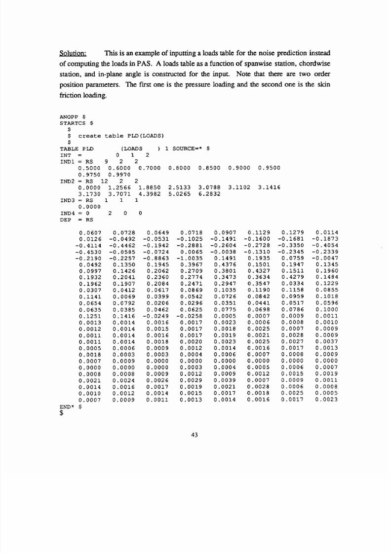
8/10/2019 NASA ANOP Propellers
http://slidepdf.com/reader/full/nasa-anop-propellers 49/104
Solution: This is an example of inputting a loads table for the noise prediction instead
of computing the loads in PAS. A loads table as a function of spanwise station, chordwise
station, and in-plane angle is constructed for the input. Note that there are two order
position parameters. The first one is the pressure loading and the second one is the skin
friction loading.
ANOPP $
STARTCS $
s
$ create table PLD(LOADS)
$
TABLE PLD (LOADS )
INT = 0 1 2
INDI = RS 9 2 2
0.50OO O.60OO O.7O00
0.9750 0.9970
IND2 = RS 12 2 2
0.0000 1.2566 1.8850
3.1730 3.7071 4.3982
IND3 = RS 1 1 1
0.0000
IND4 = 0 2 0 0
DEP = RS
0.0607
0.0126
-0.4114
-0.4530
-0.2190
0.
0492
0.0997
0 1932
0 1962
0 0307
0 1141
0 0654
0 0635
0 1251
0.0013
0.0012
0.0011
0.0011
0 .O005
0.0018
0.0007
0.0000
0.0008
0.0021
0.0014
0.0010
0.0007
END* $
S
0.0728
-0.0492
-0.4462
-0.0585
-0.2257
0.1350
0.1426
0.2041
0.1907
0.0412
0.0069
0.0792
0.0385
0 1416
0 0014
0 0014
0 0014
0 0014
0 0006
0 0003
0 0009
0 0000
0 0008
0 0024
0 0016
0.0012
0.0009
0 0649
-0 0531
-0 1942
-0 0724
-0 8863
0 1945
0 2062
0 2360
0 2084
0 0617
0.0399
0.0206
0.0462
-0.0249
0.0016
0.0015
0.0016
0.0018
0.0009
0.0003
0.0000
0.0000
0.0009
0.0026
0.0017
0.0014
0.0011
1 SOURCE =* $
0.8000 0.8500 0.9000 0.9500
2.5133 3.0788 3.1102 3.1416
5.0265 6.2832
0 0718
-0 1025
-0 2881
0 0O65
-I 0035
0 3967
0 2709
0 2774
0 2471
0 0869
0 0542
0 0296
0.0625
-0.0258
0.0017
0.0017
0.0017
0.0020
0.0012
O.OO04
0.0000
0.0003
0.0012
0.0029
0.0019
0.0015
0.0013
0.0907
-0.1491
-0.2604
-0.0038
0 1491
0 4376
0 3801
0 3473
0 2947
0 1035
0 0726
0 0351
0 0775
0.0005
0.0023
0.0018
0.0019
0.0023
0.0014
0.0006
0.0000
0.0004
0.0009
0.0039
0.0021
0.0017
0.0014
0.1129 0
-0.1600 -0
-0.2728 -0
-0.1310 -0
0.1935 0
0.1501 0
0.4327 0
0.3634 0
0.3547
0.1190
0.0842
0.0441
0.0698
0.0007
0.0006
0.0025
0.0021
0.0025
0.0016
O.OOO7
0 0000
0 OOO5
0 0012
0 00O7
0 0028
0 0018
0 0016
.1279
.1681
.3350
.2345
.0759
.1947
.1511
.4279
0.0334
0.1158
0.0959
0.0517
0.0786
0.0009
0.0008
0 0007
0 0028
0 0027
0 0017
0 0008
0 0000
0 0006
0.0015
0.0009
0.0006
0.0025
0.0017
0.0114
-0 1873
-0 4054
-0 2339
-0 0047
0 1345
0 1960
0 1484
0 1229
0 0855
0 1018
0 0596
0 i000
0 0011
0 0010
0 0009
0 0009
0 0037
0 0013
0 0009
0 0000
0.O007
0.0019
0.0011
0.0008
0.0005
0.0023
43
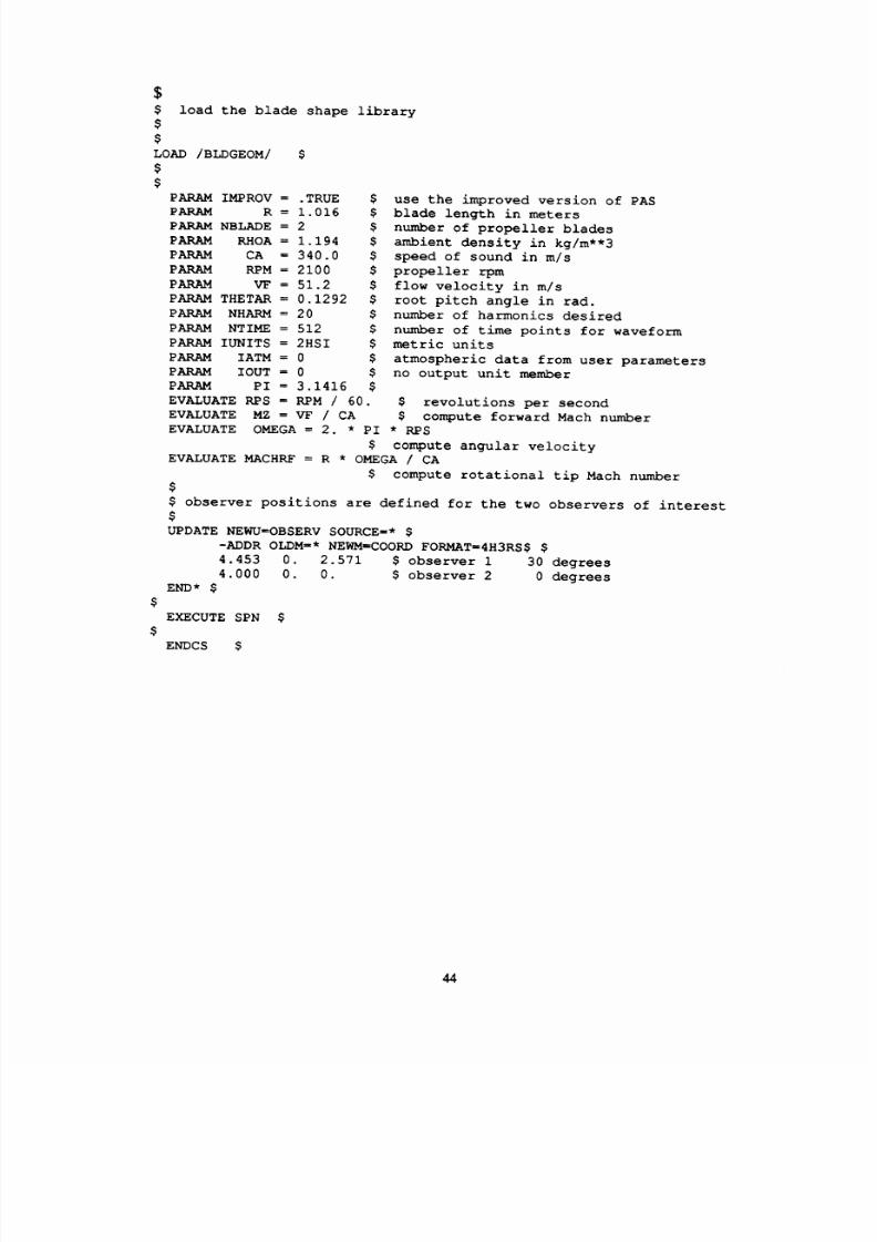
8/10/2019 NASA ANOP Propellers
http://slidepdf.com/reader/full/nasa-anop-propellers 50/104
$
$
$
$
LOAD BLDGEOM
$
$
load the blade shape
library
PARAM
IMPROV
= .TRUE
PARAM
R
=
1.016
PARAM
NBLADE =
2
PARAM
RHOA =
1.194
PARAM CA
=
340.0
PARAM RPM = 2100
PARAM VF = 51.2
PARAM THETAR = 0.1292
PARAM NHARM = 20
PARAM NTIME = 512
PARAM IUNITS = 2HSI
PARAM IATM = 0
PARAM IOUT = 0
PARAM PI = 3.1416
$ use the improved version of PAS
$ blade length in meters
$ number of propeller blades
$ ambient density in kg/m**3
$ speed of sound in
m/s
$ propeller rpm
$ flow velocity in m/s
$ root pitch angle in tad.
$ number of harmonics desired
$ number of time points for waveform
$ metric units
$ atmospheric data from user parameters
$ no output unit member
$
EVALUATE RPS = RPM 60. $ revolutions per second
EVALUATE MZ = VF CA $ compute forward Mach number
EVALUATE OMEGA = 2. * PI * RPS
$ compute angular velocity
EVALUATE MACHRF = R * OMEGA CA
$ compute rotational tip Mach number
$
$ observer positions are defined for the two observers of interest
$
UPDATE NEWU=OBSERV SOURCE=* $
-ADDR OLDM z* NEWM=COORD FORMAT=4H3RS$ $
4.453 0. 2.571 $ observer 1 30 degrees
4.000 0. 0. $ observer 2 0 degrees
END*
$
EXECUTE SPN $
ENDCS $
44

8/10/2019 NASA ANOP Propellers
http://slidepdf.com/reader/full/nasa-anop-propellers 51/104
8.3 Template 7 - Near-Field Noise Prediction
Problem:
respect to the propeller hub given by
4.453 m
0.
m
2.571m
4.000 m 0. m 0. m
at the following operating condition:
propeller RPM =
number of blades =
blade length =
inflow velocity =
root pitch angle =
Predict the noise for the two observers having x,y,z coordinates with
observer 1
observer 2
2100
2
1.016 m
51.2 m/s
0.1292 rad.
Solution: The blade geometry and the blade surface pressure are known from template
1 and template 5. The computation of the periodic acoustic pressure signature and the
spectrum of the propeller with subsonic tip speed are based on a solution of the Ffowcs
Williams-Hawkings equation without the quadrupole source term. The observers are
assumed to be moving with the aircraft and the full blade approximation is used in this
prediction.
ANOPP $
STARTCS $
$
$ observer positions are defined for the two microphones of interest
$
UPDATE NEWU=OBSERV SOURCE =* $
-ADDR OLDM=* NEWM=COORD FORMAT=4H3RS$ $
4.453 0. 2.571 $ observer 1 30 degrees from propeller plane
4.000 0. 0. $ observer 2 0 degrees or in the propeller plane
END* $
$
$ blade shape is specified by loading library BLDGEOM
$
LOAD BLDGEOM IBS IBA IBL $
$
$ Pressure and skin loadings
$
UNLOAD PLDLIB $
$
PARAM IMPROV = .TRUE $
PARAM R = 1.016 $
PARAM NBLADE = 2 $
PARAM RHOA = I. 194 $
PARAM CA = 340.0 $
PARAM RPM
=
2100 $
in the PLDLIB library
blade length in meters
number of propeller blades
ambient density in kg/m**3
speed of sound in m/s
propeller rpm
45

8/10/2019 NASA ANOP Propellers
http://slidepdf.com/reader/full/nasa-anop-propellers 52/104

8/10/2019 NASA ANOP Propellers
http://slidepdf.com/reader/full/nasa-anop-propellers 53/104
8.4 Template 8 - Noise Bubble for Far-Field Noise Prediction
Problem: This problem is similar to the problem in template 7 with the exception that
observer coordinates are input in the spherical format. In this example, the observers are
on the plane perpendicular to the propeller plane starting from the flight direction to the
back of the propeller at the following angles:
10o 30° 50 ° 90° 120 ° 150 ° 179 °
Source radius = 5 * R where R is the propeller radius
Solution: The same computational method is used in template 7. In this template,
observers are defined on an imaginary bubble which is specified by a constant radius, polar
directivity angles, and the azimuthal angles. The polar directivity angle is specified from
the front of the propeUer (0 °) to the back of the propeller (180 °) in the inflow direction. The
azimuthal angle is determined from the left hand side to right hand side of the propeller
specified from the inflow direction looking toward the propeller. A noise table is created
on the bubble which is used later by way of interpolation to evaluate the noise at specified
observers on the ground. It is important to set the parameter IOUT=2 and to input the unit
member SFIELD(THETA) and SFIELD(PHI). The source radius RX, re R is also
required.
ANOPP $
STARTCS $
$
$ the sound field arrays must be defined.
$ chosen only on the propeller plane
$
UPDATE NEWU=SFIELD SOURCE =* $
-ADDR OLDM=* NEWM=THETA FORMAT=4H*RS$ $
10. 30. 50. 90. 120. 150. 179.
-ADDR OLDM=* NEWM=PHI FORMAT=4H*RS$ $
0. .i .2 .3 .4 .5 .6 .7 .8 .9
In this case observers are
$
I. $
END* $
$
$ additional output control
$
PARAM IATM = 0
PARAM IOUT = 1
PARAM IDPDT = 1
PARAM ALPHAP = 0.020
PARAM R = 1.016
PARAM MZ = 0.157
PARAM THETAR = 0.0576
PARAM MACHRF = 0.649
PARAM CA = 342.5
PAKAM RHOA = 1.162
parameters are required
$ use atmospheric user parameters
$ generate farfield noise table in SPN
$ unsteady because of angle-of-attack
$ propeller angle-of-attack in radians
$ blade length in meters
$ flight Mach number
$ root pitch angle in radians
$ rotational tip Mach number
$ speed of sound in meters/sec
$ density in kg/meters**3
47

8/10/2019 NASA ANOP Propellers
http://slidepdf.com/reader/full/nasa-anop-propellers 54/104
$
$ the blade shape
library
is BLDGEOM and the
load library
is
PLDLIB
$
LOAD BLDGEOM/ $
LOAD PLDLIB $
$
EXECUTE SPN $
UNLOAD SPNLIB $
ENDCS $
48
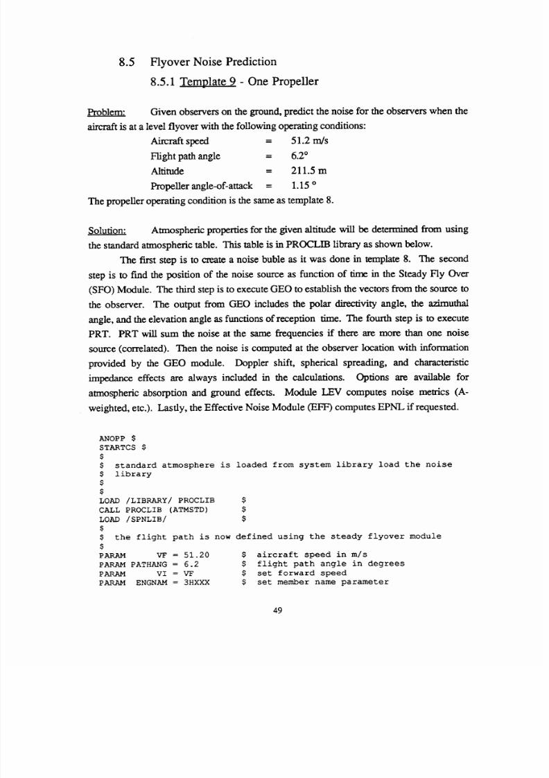
8/10/2019 NASA ANOP Propellers
http://slidepdf.com/reader/full/nasa-anop-propellers 55/104
8.5
Flyover Noise Prediction
8.5.1 Template 9 - One Propeller
Problem: Given observers on the ground, predict the noise for the observers when the
aircraft is at a level flyover with the following operating conditions:
Aircraft speed = 51.2 m/s
Flight path angle = 6.2 °
Altitude = 211.5 m
Propeller angle-of-attack = 1.15 o
The propeller operating condition is the same as template 8.
Solution: Amaospheric properties for the given altitude will be determined from using
the standard atmospheric table. This table is in PROCLIB library as shown below.
The first step is to create a noise buble as it was done in template 8. The second
step is to find the position of the noise source as function of time in the Steady Fly Over
(SFO) Module. The third step is to execute GEO to establish the vectors from the source to
the observer. The output from GEO includes the polar directivity angle, the azimuthal
angle, and the elevation angle as functions of reception time. The fourth step is to execute
PRT. PRT will sum the noise at the same frequencies if there are more than one noise
source (correlated). Then the noise is computed at the observer location with information
provided by the GEO module. Doppler shift, spherical spreading, and characteristic
impedance effects are always included in the calculations. Options are available for
atmospheric absorption and ground effects. Module LEV computes noise metrics (A-
weighted, etc.). Lastly, the Effective Noise Module (EFF) computes EPNL if requested.
ANOPP $
STARTCS $
$
$ standard atmosphere is
$ library
$
$
LOAD LIBRARY PROCLIB
CALL PROCLIB (ATMSTD)
LOAD SPNLIB
$
loaded from system library load the noise
$ the flight path is now defined using the steady flyover module
$
PARAM VF = 51.20 $ aircraft speed in m/s
PARAM PATHANG = 6.2 $ flight path angle in degrees
PARAM VI = VF $ set forward speed
PARAM ENGNAM = 3HXXX $ set member name parameter
49
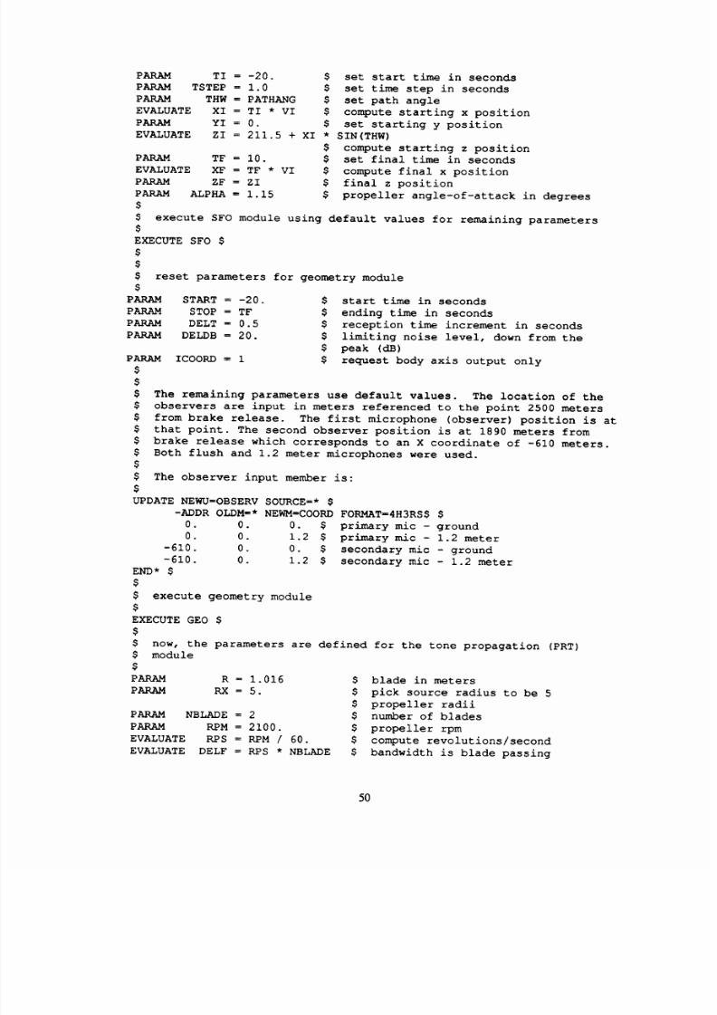
8/10/2019 NASA ANOP Propellers
http://slidepdf.com/reader/full/nasa-anop-propellers 56/104
PARAM
PARAM
PARAM
EVALUATE
PARAM
EVALUATE
PARAM TF = I0.
EVALUATE XF = TF * VI
PARAM ZF = ZI
PARAM ALPHA = 1.15
$
TI = -20. $ set start time in seconds
TSTEP = 1.0 $ set time step in seconds
THW = PATHANG $ set path angle
XI = TI * VI $ compute starting x position
YI = 0. $
set
starting y position
ZI = 211.5 + XI * SIN(THW)
$ compute starting z position
$ set final time in seconds
$ compute final x position
$ final z position
$ propeller angle-of-attack in degrees
$ execute SFO module using default values for remaining parameters
$
EXECUTE SFO $
$
$
$ reset parameters for geometry module
$
PARAM START = -20.
PARAM STOP = TF
PARAM DELT = 0.5
PARAM
DELDB
=
20.
PARAM
$
ICOORD = 1
$ start time in seconds
$ ending time in seconds
$ reception time increment in seconds
$ limiting noise
level,
down
from
the
$ peak (dB)
$ request body axis output only
The remaining
parameters
use
default
values.
The location
of
the
observers are input in meters referenced to the point 2500 meters
from brake release. The first microphone (observer) position is at
that point. The second observer position is at 1890 meters from
brake release which corresponds to an X coordinate of -610 meters.
Both flush and 1.2 meter microphones were used.
The observer input member is:
UPDATE NEWU=OBSERV SOURCE=*
-ADDR OLDM=*
NEWM=COORD FORMAT=4H3RS$ $
0. 0. 0. $
0. 0. 1.2 $
-610. 0. 0. $
-610. 0. 1.2 $
END* $
$
$ execute geometry module
$
EXECUTE GEO $
$ now, the parameters are defined for the tone propagation (PRT)
$ module
$
PARAM R
=
1.016
PAKAM RX = 5.
PARAM NBLADE = 2
PARAM RPM = 2100.
EVALUATE RPS = RPM 60.
EVALUATE DELF = RPS * NBLADE
primary
mic
- ground
primary mic - 1.2
meter
secondary mic - ground
secondary mic - 1.2 meter
$ blade in meters
$ pick source radius to be 5
$ propeller radii
$ number of blades
$ propeller rpm
$ compute revolutions/second
$ bandwidth is blade passing
50

8/10/2019 NASA ANOP Propellers
http://slidepdf.com/reader/full/nasa-anop-propellers 57/104
EVALUATE
RS
=
RX * R
PARAM SURFACE
=
4HSOFT
PARAM ABSORP = .TRUE.
PARAM
GROUND = .TRUE.
$
$ frequency
$
convert
to dimensional source
$ radius
$ soft boundary
$ predict standard absorption effect
$ predict ground effects
$ tone propagation module is executed with remaining parameters
$ defaulted
$
EXECUTE PRT YYYYYY=SPN GEOM=BODY $
$
$ the noise levels module (LEV) is executed to compute frequency
$ integrated levels. Only narrow band levels are computed.
$
PARAM NAWT=.TRUE. NDWT=.TRUE. NOSPL=.TRUE.
$ set narrow band level flags to true
PARAM IAWT=.FALSE. IDWT=.FALSE. IOSPL=.FALSE. IPNL=.FALSE.
IPNLT=.FALSE. $ set I/3-octave band level flags to false
PARAM MEMSUMN=4HPRT 4HPRES
$ define input member
$
$ the lev module is now executed
$
EXECUTE LEV $
$
EXECUTE EFF $
$
ENDCS $
8.5.2 Template 10 - Tilt Rotor
Problem: Predict the
noise for
the tilt rotor in propeller mode. This tilt rotor
has
two
identical propellers, the NACA 16 airfoil. The aerodynamic information such as lift and
drag
coefficients
are built in the library NACALB. The operating conditions are
Flight altitude
=
250 ft
Indicated airspeed
=
150 knots
Number of blades
=
4
Propeller radius = 4 ft
Propeller RPM = 1550.
Distance from each propeller hub to the centerline of the aircraft is 12.5 ft
Solution: This example is a flyover noise prediction for a tilt rotor in the propeller
mode. SPN creates a noise bubble for each propeller. A common point between the two
51
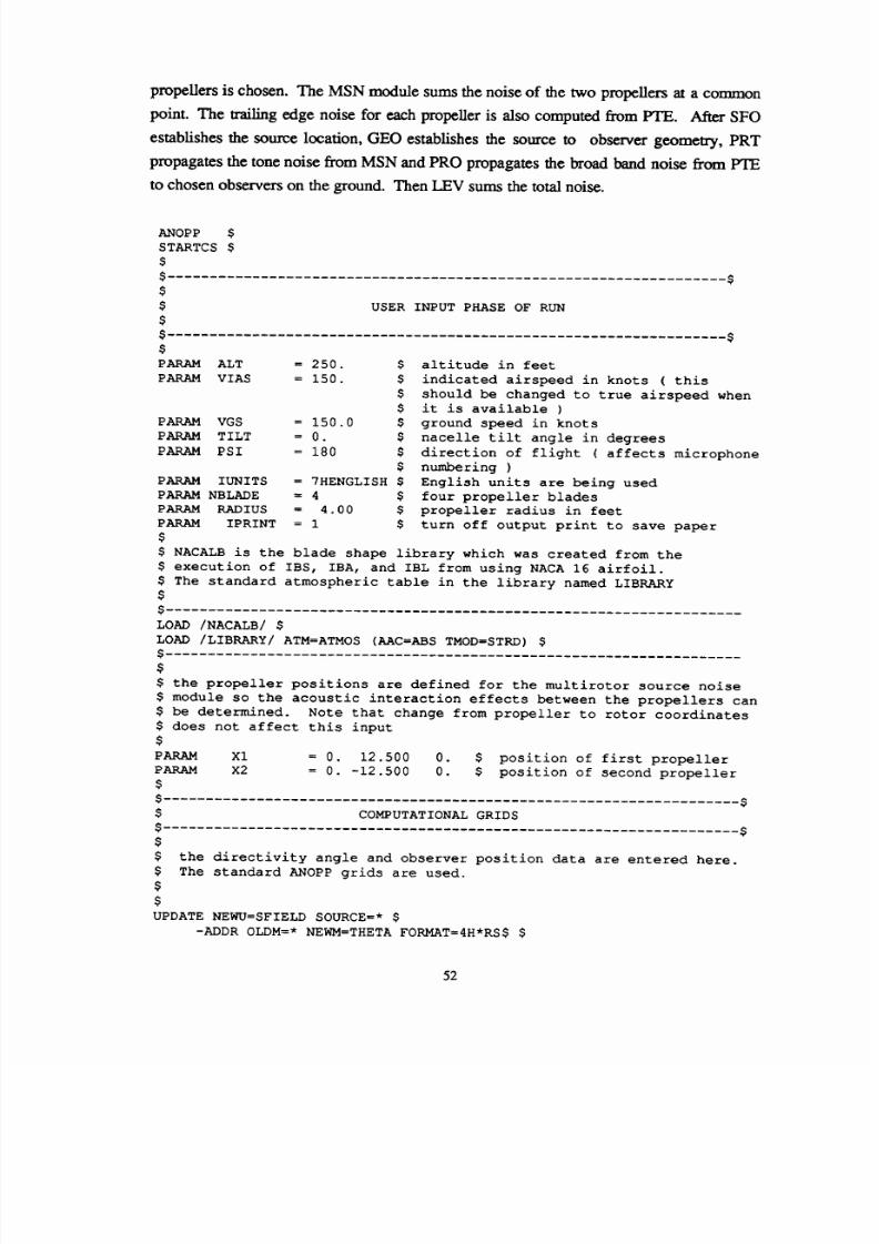
8/10/2019 NASA ANOP Propellers
http://slidepdf.com/reader/full/nasa-anop-propellers 58/104
propellersis chosen.
The
MSN module sums
the noise
of the
two propellers at a
common
point. The trailing edge noise for each propeller is also computed from PTE. After SFO
establishes the source location, GEO estabhshes the source to observer geometry, PRT
propagates the tone noise from MSN and PRO propagates the broad band noise from PTE
to chosen observers on the ground. Then LEV sums the total noise.
ANOPP $
STARTCS $
$
$
.....
USER INPUT PHASE OF RUN
$
PARAM ALT = 250.
PARAM VIAS = 150.
PARAM VGS = 150.0
PARAM TILT = 0.
PARAM PSI = 180
PARAM IUNITS = 7HENGLISH $
PARAMNBLADE = 4 $
PARAM RADIUS = 4.00 $
PARAM
IPRINT =
1
$
$ altitude in feet
$ indicated airspeed in knots ( this
$ should be changed to true airspeed when
$ it is available )
$ ground speed in knots
$ nacelle tilt angle in degrees
$ direction of flight ( affects microphone
$ numbering )
English units are being used
four propeller blades
propeller radius in feet
turn off output print to save paper
$ NACALB is the blade shape library which was created from the
$ execution of IBS, IBA, and IBL from using NACA 16 airfoil.
$ The standard atmospheric table in the library named LIBRARY
$
$
LOAD NACALB $
LOAD LIBRARY ATM=ATMOS (AAC=ABS TMOD=STRD) $
$
$
$ the propeller positions are defined for the multirotor source noise
$ module so the acoustic interaction effects between the propellers can
$ be determined. Note that change from propeller to rotor coordinates
$ does not affect this input
$
PARAM Xl = 0. 12.500 0. $ position of first propeller
PARAM X2 = 0. -12.500 0. $ position of second propeller
$
$
-----$
COMPUTATIONAL GRIDS
-$
$
$ the directivity angle and observer position data are entered here.
$ The standard ANOPP grids are used.
$
$
UPDATE NEWU=SFIELD SOURCE =* $
-ADDR OLDM=* NEWM=THETA FORMAT=4H*RS$ $
52
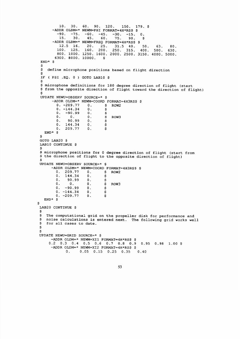
8/10/2019 NASA ANOP Propellers
http://slidepdf.com/reader/full/nasa-anop-propellers 59/104
i0. 30. 60. 90. 120. 150. 179. $
-ADDR OLDM=* NEWM=PHI FORMAT=4H*RS$ $
-90. -75. -60. -45. -30. -15. 0.
15. 30. 45. 60. 75. 90. $
-ADDR OLDM=* NEWM=FREQ FORMAT=4H*RS$ $
12.5 16. 20. 25. 31.5 40. 50. 63. 80.
100. 125. 160. 200. 250. 315. 400. 500. 630.
800. 1000. 1250. 1600. 2000. 2500. 3150. 4000. 5000.
6300. 8000. 10000. $
END* $
$
$ define microphone positions based on flight direction
$
IF ( PSI .EQ. 0 ) GOTO LAB10 $
$
$ microphone definitions for 180 degree direction of flight (start
$ from the opposite direction of flight toward the direction of flight)
$
UPDATE NEWU=OBSERV SOURCE=* $
-ADDR OLDM=* NEWM=COORD FORMAT=4H3RS$ $
0
0
0
0
0
0
0
END* $
$
-209.77
-144.34
-90.99
0.
90.99
144.34
209.77
0
$ ROW2
0 $
0
$
0 $ ROW3
0 $
0 $
0 $
GOTO LAB20 $
LAB10
CONTINUE $
$
$ microphone positions for 0 degree direction of flight (start from
$ the direction of flight to the opposite direction of flight)
$
UPDATE NEWU=OBSERV SOURCE=* $
-ADDR OLDM=* NEWM=COORD FORMAT=4H3RS$ $
0. 209.77 0. $ ROW2
0. 144.34 0. $
0. 90.99 0. $
0. 0. 0. $ ROW3
0. -90.99 0. $
0. -144.34 0. $
0. -209.77 0. $
END*
$
$
LAB20 CONTINUE $
$
The computational grid on the propeller disk for performance and
noise calculations is entered next. The following grid works well
0.95 0.98 1.00 $
0.40
$
$
$ for all cases to date.
$
$
UPDATE NEWU=GRID SOURCE =* $
-ADDR OLDM=* NEWM=XII FORMAT=4H*RS$ $
0.2 0.3 0.4 0.5 0.6 0.7 0.8 0.9
-ADDR OLDM=* NEWM=XI2 FORMAT=4H*RS$ $
0. 0.05 0.15 0.25 0.35
53

8/10/2019 NASA ANOP Propellers
http://slidepdf.com/reader/full/nasa-anop-propellers 60/104
0.45 0.50 0.55 0.60 0. 625
0.70 0.75 0.80 0.85 0.90
-ADDR OLDM=* NEWM=PSI FORMAT=4H*RS$
0.00
END* $
$
$
0.65
0.95 1.00 $
DERIVED AND STANDARD USER PARAMETERS
$
$
$
PARAM IMPROV = .TRUE.
PARAM CA = 1115.49
PARAM ALPHAP = TILT
PARAM IDPDT = 0
PARAM NBLADE = 4
PARAM PI =
3.1415927
PARAM
RPM = 1550.
$ improved blade section modules are used
$ speed of sound in ft/sec
$ set propeller angle-of-attack to tilt
$ angle
$ propeller loading is steady
$ number of propeller blades
$ define value of pi
$ propeller RPM
EVALUATE OMEGA = RPM * PI 30.
$ compute propeller angular velocity
EVALUATE MACHRF = OMEGA * RADIUS CA
$ compute propeller hover tip Mach number
EVALUATE KNTFPS = 0.5144444 .3048
$ conversion factor from knots to
$ feet/sec
EVALUATE MZ = VIAS * KNTFPS CA
$ compute propeller relative forward
$ speed
= RADIUS * 2. $ compute propeller diameter
= RPM 60. $ compute revolutions per second
EVALUATE D
EVALUATE RPS
$
$
$
EVALUATE
RS
=
I0. * RADIUS
PARAM R1 = RADIUS
PARAM R2
=
RADIUS
PARAM IOPT = 2
$
$ SPN module
here the inputs for the first execution of the MSN module are set up
$
PARAM METHOD
=
1
PARAM IOUT = 2
PARAM NTIME = 128
PARAM NHARM = 16
PARAM RX =
5.
$
$ SFO module
$
PARAM ENGNAM
$ compute dimensional observer distance
$ radius of first propeller
$ radius of second propeller
$ propeller coordinate system option
PARAM TSTEP
=
i.
EVALUATE VI
EVALUATE XI
$ use line
source
method to
save
time
$ request near field noise analysis
use 128
time points in time history
$ request 32 harmonics
$ set propeller source radius to five
$ diameters
= 3HXXX $ change value of engnam to match default
$ values of other modules
$ data generated at 1 second intervals
= VGS * KNTFPS
$ convert forward speed to feet/sec
= - ALT SIN 15. )
$ start flight path at polar directivity
$ of 15 degrees
54

8/10/2019 NASA ANOP Propellers
http://slidepdf.com/reader/full/nasa-anop-propellers 61/104
EVALUATE START = XI VI
PARAM TI = START
EVALUATE XF
EVALUATE
TF
PARAM VF
$
$ GEO module
$
EVALUATE AW
$
$
$
= -i. * XI $
$
=
-I. * START $
= VI $
PARAM WEIGHT = 12872.
EVALUATE
MASSAC
= PI * RADIUS**2
$
$
PARAM
DTIME
=
0.5
PARAM
ICOORD =
1
$
$ PRO and PRT modules
$
EVALUATE DELF
PARAM SURFACE
PARAM ABSORP
PARAM GROUND
$
$ LEV module
$
PARAM IAWT
PARAM IDWT
PARAM
IOSPL
PARAM IPNL
PARAM IPNLT
PARAM NAWT
PARAM NDWT
PARAM NOSPL
$
set start time of flight path
start is a geo parameter - it is
changed by SFO so both are set here
final flight path distance set at same
distance past overhead
corresponding final time
final velocity
aircraft reference area in square feet
= WEIGHT 32.174
$ compute mass of aircraft in slugs
$ compute in 1/2 second increments for
$
EPNL
calculations
$ request body axis coordinate system
= OMEGA * NBLADE 2. PI
$ the propeller bandwidth is the
$ fundamental frequency
= 4HHARD $ microphones were on hard surfaces
= .TRUE. $ request atmospheric absorption effects
$ be applied to the data
=
.TRUE. $
request ground effects
be applied to the
$ data
=
.TRUE. $
= .FALSE. $
= .TRUE. $
= .TRUE. $
= .TRUE. $
=
.FALSE. $
= .FALSE. $
=
.FALSE. $
$ bring the load libraries
$
LOAD PLDLIB/ $
$
$
set flags for metric calculations
MODULE
EXECUTION
PHASE OF RUN
$
$ now, the MSN module is executed
$
EXECUTE MSN OBSERV=DUMMY $
$
$ the SPN module is executed for the first propeller using the name
$ overrides for the first propeller.
$
$
$
55
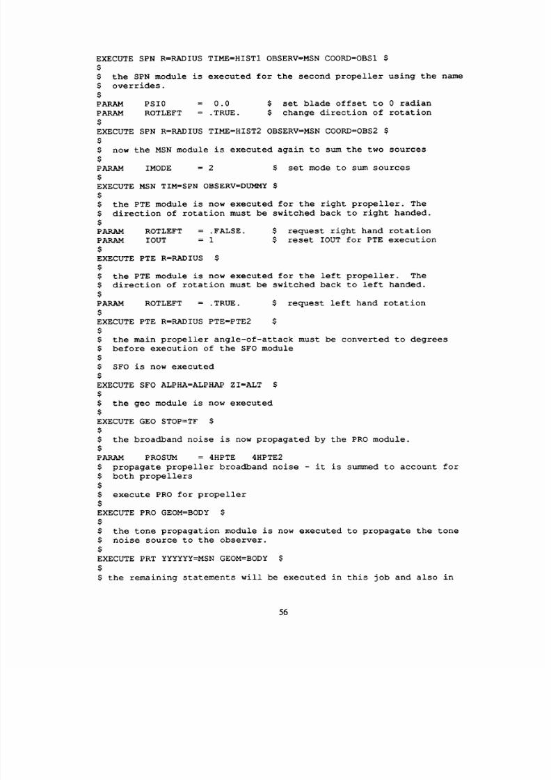
8/10/2019 NASA ANOP Propellers
http://slidepdf.com/reader/full/nasa-anop-propellers 62/104
EXECUTE SPN R=RADIUS TIME=HISTI OBSERV=MSN COORD=OBSI $
$
$ the SPN module is executed for the second propeller using the name
$ overrides.
$
PARAM PSI0 = 0.0 $ set blade offset to 0 radian
PARAM ROTLEFT = .TRUE. $ change direction of rotation
$
EXECUTE SPN R=RADIUS TIME=HIST2 OBSERV=MSN COORD=OBS2 $
$
$ now the MSN module is executed again to sum the two sources
$
PARAM IMODE = 2 $ set mode to sum sources
$
EXECUTE MSN TIM=SPN OBSERV=DUMMY $
$
$ the PTE module is now executed for the right propeller. The
$ direction of rotation must be switched back to right handed.
$
PARAM ROTLEFT = .FALSE. $ request right hand rotation
PARAM IOUT = 1 $ reset IOUT for PTE execution
$
EXECUTE PTE R=RADIUS $
$
$ the PTE module is now executed for the left propeller. The
$ direction of rotation must be switched back to left handed.
$
PAKAM ROTLEFT = .TRUE. $ request left hand rotation
$
EXECUTE PTE R=RADIUS PTE=PTE2 $
$
$ the main propeller angle-of-attack must be converted to degrees
$ before execution of the SFO module
$
$ SFO is now executed
$
EXECUTE SFO ALPHA=ALPHAP ZI=ALT $
$
$ the geo module is now executed
$
EXECUTE GEO STOP=TF $
$
$ the broadband noise is now propagated by the PRO module.
$
PARAM PROSUM = 4HPTE 4HPTE2
$ propagate propeller broadband noise - it is summed to account for
$ both propellers
$
$ execute PRO for propeller
$
EXECUTE PRO GEOM=BODY $
$
$ the tone propagation module is now executed to propagate the tone
$ noise source to the observer.
$
EXECUTE PRT YYYYYY=MSN GEOM=BODY $
$
$ the remaining statements will be executed in this job and also in
56

8/10/2019 NASA ANOP Propellers
http://slidepdf.com/reader/full/nasa-anop-propellers 63/104
the restart job that propagates tone noise predictions. The noise
levels (LEV)
module is now
executed to
compute
the frequency
$ integrated levels and to sum noise sources. The parameter MEMSUMN
$ has the unit member name of the PRT output to be summed. Note
$ that all names in MEMSUMN must have the same hollerith length.
$ Similarly the user parameter memsum has the names of the PRO output.
$
PARAM IPRINT
= 3
PARAM MEMSUMN = 4HPRT
PARAM MEMSUM
=
4HPRO
$ turn on output print for total noise
4HPRES
$ propagate tone noise source
4HPRES
$ propagate broadband noise source
$
$ the lev module
is
now executed
$
EXECUTE LEV LEV=LEVTOT $
$
$ the source summed 1/3 octave band spectra are written to the
$ external file finally the effective noise module is executed
$
EXECUTE EFF LEV=LEVTOT $
$
$ the job is
finished
$
PROCEED $
ENDCS $
57

8/10/2019 NASA ANOP Propellers
http://slidepdf.com/reader/full/nasa-anop-propellers 64/104
9. PAS Prediction and Measured Data
9.1 PAS Prediction Results
9.1.1 Four Methods from SPN
The results from using the different options in the Subsonic Propeller Noise (SPN)
module
is presented and compared with measured data. In general, the predictions from
the four methods are very close for the first few harmonics, but for higher harmonics, the
discrepancy increases. These options permit greater compatibility with users computer
resources. The full blade
surface
method uses the
most
CPU time compared to the
other
methods and the point source approximation uses the least amount of CPU time.
Figure 7 illustrates the DNW tunnel configuration along with 2 chosen
microphones. Predictions from the four methods are shown in figures 8, 9 and 10. Data
available for the comparison is obtained from reference 8. Operating conditions for the
predictions are as follows:
Run RIM Flow Vel. Attitude Total Mach
number m/s Angle (deg.)
number
BN4 2100 51.2 0. 0.67
GN3 2700 77.0 -7.4 0.87
EN2 2400 51.9 7.3 0.77
9.1.2 Synchrophasing Using PAS
Synchrophasing was studied using PAS to determine the effects of blade phase
angle for a tilt rotor in the propeller mode. In template 9, note that there is one blade offset
parameter name PSI0. This parameter is to input the blade offset angle (phase) for the
study of the effect of the blade phasing angle in the tilt rotor case.
Propeller geometry:
• NACA 16 series blade
• 8 feet diameter
• 25 ft hub to hub separation
• Each propeller has 4 blades
58
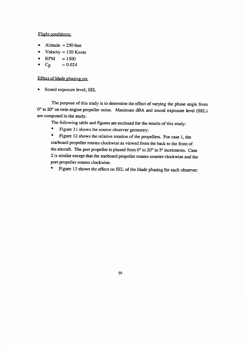
8/10/2019 NASA ANOP Propellers
http://slidepdf.com/reader/full/nasa-anop-propellers 65/104
Flight conditions:
* Altitude = 250 feet
• Velocity = 150 Knots
• RPM = 1500
• Cp = 0.024
Effect of blade phasing on;
• Sound exposure level, SEL
The purpose of this study is to determine the effect of varying the phase angle from
0 ° to 20 ° on twin engine propeller noise. Maximum dBA and sound exposure level (SEL)
are computed in the study.
The following table and figures are enclosed for the results of this study:
* Figure 11 shows the source observer geometry.
* Figure 12 shows the relative rotation of the propellers. For case 1, the
starboard propeller rotates clockwise as viewed from the back to the front of
the aircraft. The port propeller is phased from 0 ° to 20 ° in 5 ° increments. Case
2 is similar except that the starboard propeller rotates counter clockwise and the
port propeller rotates clockwise.
* Figure 13 shows the effect on SEL of the blade phasing for each observer.
59
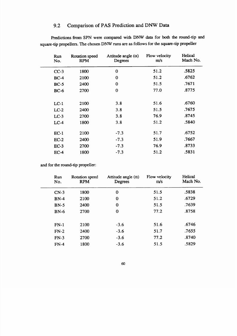
8/10/2019 NASA ANOP Propellers
http://slidepdf.com/reader/full/nasa-anop-propellers 66/104
9.2 Comparison of PAS Prediction and DNW Data
Predictions from SPN were
compared
with
DNW
data
for
both the round-tip
square-tip propellers. The chosen DNW runs are as follows for the square-tip propener
Run Rotation
speed Attitude angle (or) Flow velocity
Helical
No. RPM Degrees m/s Mach No.
and
CC-3 1800 0 51.2 .5825
BC-4 2100 0 51.2 .6762
BC-5 2400 0 51.5 .7671
BC-6 2700 0 77.0 .8775
LC-1 2100 3.8 51.6 .6760
LC-2 2400 3.8 51.5 .7675
LC-3 2700 3.8 76.9 .8745
LC-4 1800 3.8 51.2 .5840
EC-1 2100 -7.3 51.7 .6752
EC-2 2400 -7.3 51.9 .7667
EC-3 2700 -7.3 76.9 .8733
EC-4 1800 -7.3 51.2 .5831
and for the round-tip
propeller:
Run Rotation speed Attitude angle (00 Flow velocity Helical
No. RPM Degrees m/s Mach No.
CN-3 1800 0 51.5 .5838
BN-4 2100 0 51.2 .6729
BN-5 2400 0 51.5 .7639
BN-6 2700 0 77.2 .8758
FN-1 2100 -3.6 51.6 .6746
FN-2 2400 -3.6 51.7 .7655
FN-3 2700 -3.6 77.2 .8740
FN-4 1800 -3.6 51.5 .5829
60

8/10/2019 NASA ANOP Propellers
http://slidepdf.com/reader/full/nasa-anop-propellers 67/104
GN- 1 2100 7.4 51.4 .6751
GN-2 2400 7.4 51.7 .7664
GN-3 2700 7.4 77.0 .8735
GN-4 1800 7.4 51.2 .5830
The microphone configuration is shown in figure 14. The five chosen microphones
are microphones 2, 4, 6, 8, 9. The angles-of-attack for the round-tip propeller are 0 °,
-3.6 ° , and 7.4 ° . For the square-tip propeller, the chosen angles-of-attack are 0 ° , 3.8 °, and
-7.3 ° . The positive angle means that the propeller is nose down to the microphone array
and the negative angle it is nose up.
Figures 15 to 18 show the comparison of the PAS and DNW data for the round-tip
propeller for microphones 2 and 4 for 1800, 2100, 2400, and 2700 RPM and the attitude
angles are 0 °, -3.6 °, and 7.4 °. Figures 19 to 22 are also for the round-tip propeller at the
angles-of-attack -3.6 ° and 7.4 ° for microphones 6, 8, and 9. Figure 19 is for 1800 RPM,
figure 20 is for 2100 RPM, figure 21 is for 2400 RPM, and figure 22 is for 2700 RPM.
Figures 23 to 30 depict the results for the square-tip propeller for the same operating
conditions. The comparisons of PAS predictions and DNW data for the round-tip propeller
seem to be better than for the square-tip propeller, especially at high RPM.
61
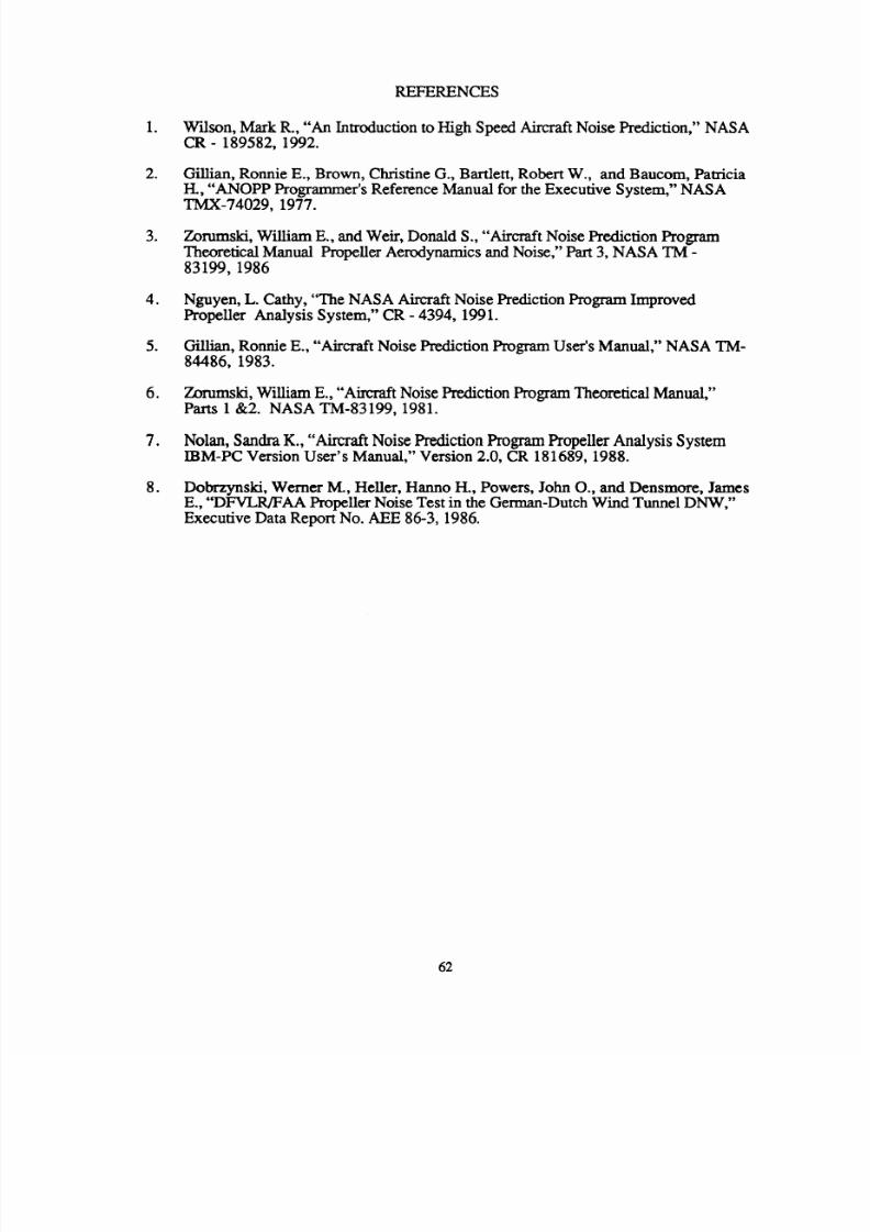
8/10/2019 NASA ANOP Propellers
http://slidepdf.com/reader/full/nasa-anop-propellers 68/104
o
.
.
°
.
.
7_
.
REFERENCES
Wilson, Mark R., "An Introduction to High Speed Aircraft Noise Prediction," NASA
CR- 189582, 1992.
Ginian, Ronnie E., Brown, Christine G., Bartlett, Robert W., and Baucom, Patricia
I-L, "ANOPP Programmer's Reference Manual for the Executive System," NASA
TMX-74029, 1977.
Zonmaski, William E., and Weir, Donald
S.,
"Aircraft Noise Prediction Program
Theoretical Manual Propeller Aerodynamics and Noise," Part 3, NASA TM -
83199, 1986
Nguyen,
L. Cathy, "The NASA Aircraft Noise Prediction Program Improved
Propeller Analysis System," CR - 4394, 1991.
Gillian, Ronnie E., "Aircraft Noise Prediction Program User's Manual," NASA TM-
84486, 1983.
Zorumski, William E., "Aircraft Noise Prediction Program Theoretical Manual,"
Parts 1 &2. NASA TM-83199, 1981.
Nolan, Sandra K., "Aircraft Noise Prediction Program Propeller Analysis System
IBM-PC Version User's Manual," Version 2.0, CR 181689, 1988.
Dobrzynski, Werner M.,
Heller, Harm, H.,
Powers, John O., and Densmore, James
E., "DFVLR/FAA Propeller Noise Test in the German-Dutch Wind Tunnel DNW,"
Executive Data Report No. AEE 86-3, 1986.
62
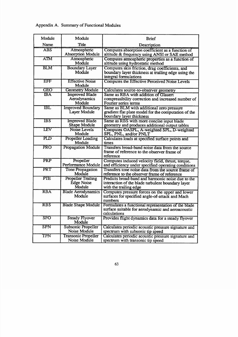
8/10/2019 NASA ANOP Propellers
http://slidepdf.com/reader/full/nasa-anop-propellers 69/104
AppendixA. Summaryof FunctionalModules
Module
Name
ABS
ATM
BLM
EFF
GEO
IBA
IBL
IBS
LEV
PLD
PRO
Module
rifle
Atmospheric
Absorption Module
Atmospheric
Module
Boundary Layer
Module
Effective Noise
Module
Geometr
7
Module
Improved Blade
Aerodynamics
Module
Improved Boundary
Layer Module
Improved Blade
Shape Module
Noise Levels
Module
Propeller Loading
Module
Propagation Module
PRP Propeller
Performance Module
PRT
FI'E
RBA
RBS
SFO
SPN
TPN
Tone Propagation
Module
Propeller Trailing
Edge Noise
Module
Blade Aerodynamics
Module
Blade Shape Module
Steady Flyover
Module
Subsonic Propeller
Noise Module
Transonic Propeller
Noise Module
Brief
Description
Computes absorption coefficient as a function of
altitude & frequency
usin_
ANSI
or
SAE method
Computes atmospheric properties as a function of
altitude using hydrostatic method
Computes skin friction, drag coefficients, and
boundary layer thickness at trailing edge using the
inte_g'al formulations
Computes the Effective Perceived Noise Levels
Calculates source-to-observer _eometr_¢
Same as RBA with addition of Glauert
compressibility correction and increased number of
Fourier series terms
Same as BLM with additional zero pressure
gradient flat plate model for the computation of the
boundary layer thickness
Same as RBS with more concise input blade
_eometry and produces additional output tables
Computes OASPL, A-weighted SPL, D-weighted
SPL, PNL, and/or PNLT
Calculates loads at specified surface points and
times
Transfers broad-band noise
data
from the source
frame of reference to the observer fl'ame of
reference
Computes induced velocity field, thrust, torque,
and efficiency under specified opemtin_ conditions
Transfers tone noise data from the source frame of
reference to the observer frame of reference
Predicts broad-band and harmonic noise due to the
interaction of the blade turbulent boundary layer
with the trailin_ edge
Computes pressure forces on the upper and lower
surfaces for specified angle-of-attack and Mach
numbers
Formulates a functional representation of the blade
surface suitable for aerodynamic and aeroacoustic
calculations
Provides flight dynamics data for a steady flyover
Calculates periodic acoustic pressure signature and
spectrum with subsonic tip speed
Calculates periodic acoustic pressure signature and
spectrum with transonic tip speed
63

8/10/2019 NASA ANOP Propellers
http://slidepdf.com/reader/full/nasa-anop-propellers 70/104
Appendix
B.
- TABLE
Control
Statement Discussion
The TABLE control statement builds an ANOPP data table which can be used as
input to the following functional modules. What follows is a brief description of the
elements
of
a
table control
statement
and how these
elements
fit together to form a usable
ANOPP table. For more detailed information refer to Section 3.7.3 of reference 2.
Fo_at: Type 1 Tables (only type currently available).
A table is generally has the following format:
TABLE UNIT(MEMBER) 1 SOURCE=* $
INT=0,1,2
IND l=RS,n 1,2,2, independent variable values separated by commas or blanks
IND2=RS,n2,2,2, independent variable values separated by commas or blanks
IND3=RS,n3,2,2, independent variable values separated by commas or blanks
IND4=RS,n4,2,2, independent variable values separated by commas or blanks
DEP=RS, dependent variable values separated by commas or blanks
END* $
The first word of the first line is TABLE following the data unit member names.
Number 1 shows that type one table is currently available. SOURCE= specifies where the
data is located from which the table will be built. The * indicates that the data will
immediately follow the TABLE control statement. As with any ANOPP control statement,
this line must end with a dollar sign symbol ($).
The line beginning with INT determines which interpolation procedures will be
permitted in this table. A 0 indicates no interpolation, a 1 indicates linear interpolation, and
a 2 indicates cubic-spline interpolation.
The next four lines define the independent variables (IND). The maximum for the
independent variable types is four. Each of the independent variable cards has the
following descriptions:
RS : real single precision
The first number is the number of independent variables in that line
The second integer number is the interpolation code for the extrapolation
procedure to be used if the specified value for this independent variable falls
beyond the last table value for the independent variable.
64
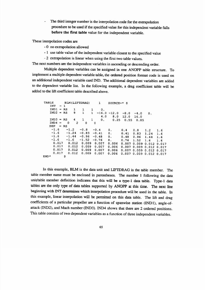
8/10/2019 NASA ANOP Propellers
http://slidepdf.com/reader/full/nasa-anop-propellers 71/104
Thethird integernumbers theinterpolationcodefor theextrapolation
procedureo beusedf thespecifiedvaluefor thisindependentariablefalls
beforethe first table valuefor the independentvariable.
These interpolation codes are
- 0 no extrapolation
allowed
- 1 use table value of the independent variable closest
to
the specified value
- 2 extrapolation is linear when using the first two table values.
The
next numbers are the
independent
variables in amending or descending order.
Multiple dependent variables can
be
assigned
in
one ANOPP table
structure.
To
implement a multiple dependent variable table, the ordered position format code is used on
an additional independent variable card IND. The additional dependent variables are added
to the dependent variable list. In the following example, a drag coefficient table will be
added to the lift coefficient table described above.
TABLE BLM (L IFTDRAG)
INT = 1
INDI
= RS 1 1
IND2 = RS 9 1
1 SOURCE =* $
1 0.
1 -16.0 -12.0 -8.0 -4.0
4.0 8.0 12.0 16.0
IND3 = RS 4 1 1 0. 0.25 0.55 0.85
IND4 = 0 2 0 0
DEP = RS
-I. 6 -1.2 -0.8 -0.4 0. 0.4 0.8
-1.6 -1.24 -0.83 -0.41 0. 0.41 0.83
-1.6 -1.44 -0.96 -0.48 0. 0.48 0.96
-1.6 -1.6 -1.52 -0.76 0. 0.76 1.52
0.017 0.012 0.009 0.007 0.006 0.007 0.009
0.017 0.012 0.009 0.007 0.006 0.007 0.009
0.017 0.012 0.009 0.007 0.006 0.007 0.009
0.017 0.012 0.009 0.007 0.006 0.007 0.009
END* $
0 •
1.2 1.6
1.24 1.6
1.44 1.6
1.6 1.6
0.012
0.017
0.012 0.017
0.012 0.017
0.012 0.017
In
this example,
BLM
is the data unit and LIFTDRAG is the table
member.
The
table member name must be enclosed in parentheses. The number 1 following the data
unit/table member definition indicates that this will be a type-1 data table. Type-1 data
tables are the only type of data tables supported by ANOPP at this time. The next line
beginning with INT determines which interpolation procedure will be used in the table. In
this example, linear interpolation will be permitted on this data table. The lift and drag
coefficients of a particular propeller are a function of spanwise station (IND1), angle-of-
attack (IND2), and Mach number (IND3). IND4 shows that there are 2 ordered positions.
This table consists of two dependent variables as a function of three independent variables.
65
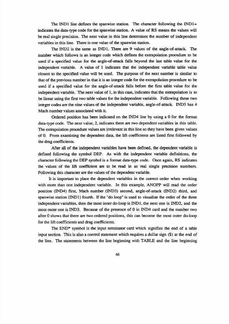
8/10/2019 NASA ANOP Propellers
http://slidepdf.com/reader/full/nasa-anop-propellers 72/104
The IND 1 line defines the spanwise station. The character following the IND 1=
indicates the data-type code for the spanwise station. A value of RS means the values will
be real single precision. The next value in this line determines the number of independent
variables in this line. There is one value of the spanwise station.
The IND2 is the same as IND 1. There are 9 values of the angle-of-attack. The
number
which follows
is
an
integer
code
which defines
theextrapolationrocedure to
be
used if
a
specifiedvalue
for the angle-of-attackalls
beyond
the
last
table
value
for the
independentvariable. A value of 1 indicatesthatthe independent variabletablevalue
closestto thespecifiedvalue willbe used. The purpose of the nextnumber issimilarto
that
of
the previous number in that
it
is an integer
code for
the extrapolation procedure to be
used if a specified value for the angle-of-attack falls before the first table value for the
independent variable. The next value of 1, in this case, indicates that the extrapolation is to
be linear using the first two table values for the independent variable. Following these two
integer codes are the nine values of the independent variable, angle-of-attack. IND3 has 4
Mach number values associated with it.
Ordered position has been indicated on the IND4 line by using a 0 for the format
data-type code. The next value, 2, indicates there are two dependent variables in this table.
The extrapolation procedure values are irrelevant in this line so they have been given values
of 0. From examining the dependent data, the lift coefficients are listed fast followed by
the drag coefficients.
After all of the independent variables have been defined, the dependent variable is
defined following the symbol DEP. As with the independent variable definitions, the
character following the DEP symbol is a format data-type code. Once again, RS indicates
the values of the lift coefficient
are
to be read in as real single precision numbers.
Following this character are the values of the dependent variable.
It is important to place the dependent variables in the correct order when working
with more than one independent variable. In this example, ANOPP will read the order
position (IND4) first, Mach number (IND3) second, angle-of-attack (IN'D2) third, and
spanwise station (IND 1) fourth. If the "do loop" is used to visualize the order of the three
independent variables, then the most inner do-loop is IND 1, the next one is IND2, and the
most outer one is IND3. Because of the presence of 0 in IND4 card and the number two
after 0 shows that there are two ordered positions, this can become the most outer do-loop
for the lift coefficients and drag coefficients.
The END* symbol is the input terminator card which signifies the end of a table
input section. This is also a control statement which requires a dollar sign ($) at the end of
the line. The statements between the line beginning with TABLE and the line beginning
66

8/10/2019 NASA ANOP Propellers
http://slidepdf.com/reader/full/nasa-anop-propellers 73/104
with END* are table description cards, not control statements, therefore, they do not
require dollar sign symbols ($) at the end of each line.
67

8/10/2019 NASA ANOP Propellers
http://slidepdf.com/reader/full/nasa-anop-propellers 74/104
Z
°,F,,4
611

8/10/2019 NASA ANOP Propellers
http://slidepdf.com/reader/full/nasa-anop-propellers 75/104
®rs_
@13o--1
@Fa
®
NO
NO _ YES
Figure 2.
®
Flowchart of ANOPP-PAS program modules used for wind
tunnel and flight predictions
@
69

8/10/2019 NASA ANOP Propellers
http://slidepdf.com/reader/full/nasa-anop-propellers 76/104
:g
:g
PURPOSE
-
short description of the functional module
AUTHOR
-
programmer's initials and level number, such as LO1/O0/O0
INPUT
USER PARAMETERS
Namel - description
Name n - description
REAL USER PARAMETER LIMITS - SI UNITS
PARAMETER MINIMUM MAXIMUM DEFAULT
Name 1 number number number
Namen number number number
REAL USER PARAMETER LIMITS - ENGLISH UNITS
PARAMETER MINIMUM MAXIMUM DEFAULT
Name 1 number number number
Namen number number number
INTEGER/LOGICAL/ALPHA PARAMETER UNITS
PARAMETER MINIMUM MAXIMUM DEFAULT
Name 1 number number number
Namen number number number
MEMBERS
DATA UNIT(DATA MEMBER)
TEMPORARIES
MEMBERS
DATA UNIT(DATA MEMBER)
OUTPUT
SYSTEM PARAMETERS
Name - description
USER PARAMETERS - same as for iNPUT
MEMBERS
DATA UNIT(DATA MEMBER)
70
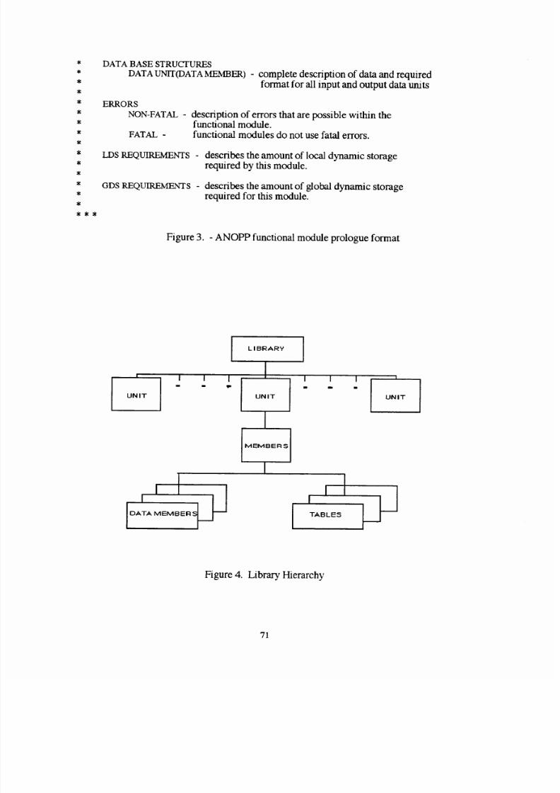
8/10/2019 NASA ANOP Propellers
http://slidepdf.com/reader/full/nasa-anop-propellers 77/104
DATA BASE STRUCTURES
DATA UNE(DATA MEMBER) - complete description of data and required
format for all input and output data units
ERRORS
NON-FATAL -
FATAL -
description of errors
that
are possible within
the
functional module.
functional modules do not use fatal errors.
LDS
REQUIREMENTS -
describes the amount of local dynamic storage
required by this module.
GDS
REQUIREMENTS -
describes the amount of global dynamic storage
required for this module.
Figure 3. - ANOPP functional module prologue format
|
I
l 1
NIT
LIBRARY
I
I
ii
DATA MEMBER S/
TABLES
I
UNIT
Figure 4. Library Hierarchy
71
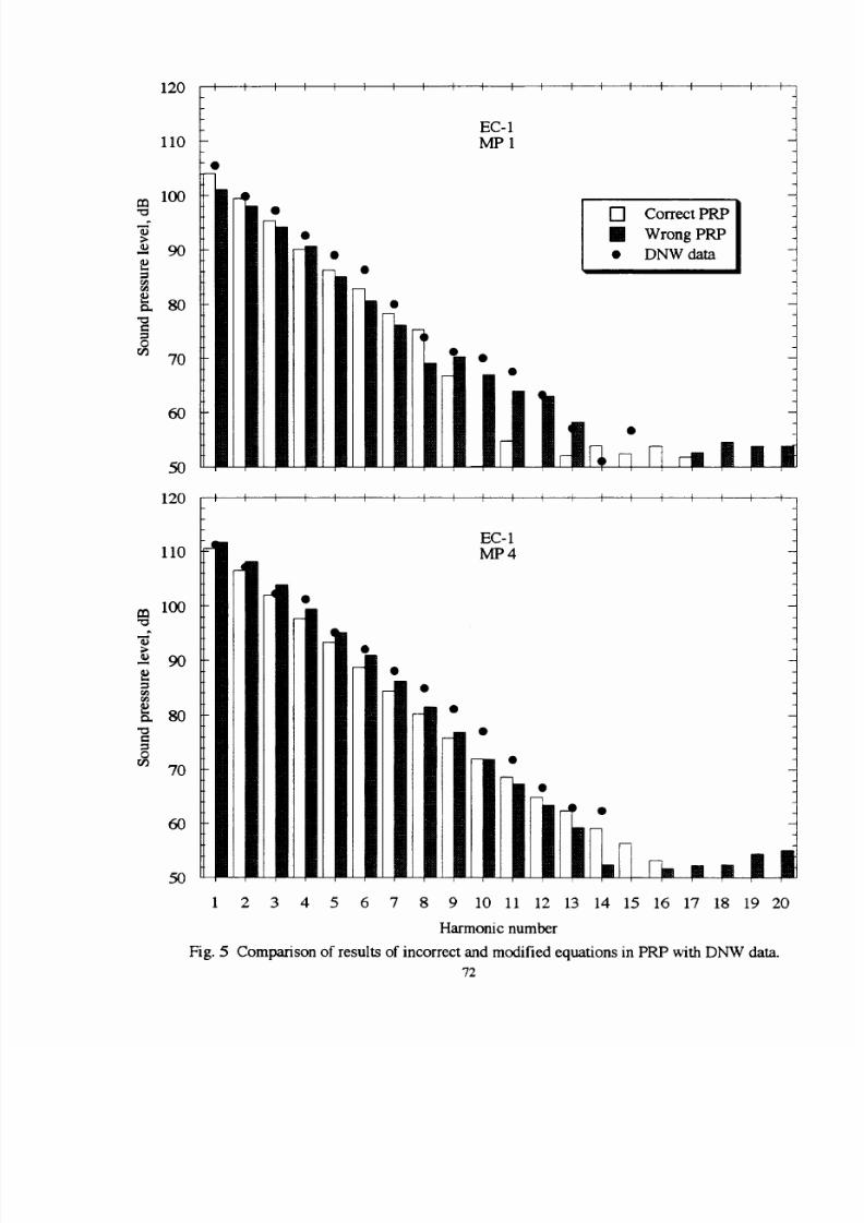
8/10/2019 NASA ANOP Propellers
http://slidepdf.com/reader/full/nasa-anop-propellers 78/104
m
_2
I=
0
09
m
m
:1
t_
0
r._
120
110
100
9O
80
70
6O
50
120
110
100
90
80
7O
6O
5O
Fig. 5
I I I I I I I
I
t I I
I
L I I I J I
I
EC-1
MP1
[] Correct PRP
m Wrong PRP
•
DNW dam
EC-1
MP4
2 3 4 5 6 7 8 9 10 11 12 13 14 15 16 17 18 19 20
Harmonic number
Comparison of results of incorrect and modified equations in PRP with DNW data.
72

8/10/2019 NASA ANOP Propellers
http://slidepdf.com/reader/full/nasa-anop-propellers 79/104
x 1
x__iu__: _ F_mo,
->< -,,L.x
Blade Fixed Reference "%,,../"/]] _,_-"¢'- ,,, .., ...
x;- v=_ x_ .
r12
Fig. 6 Reference frames.
_Observer
1
"_ __ Observer2
\ F--
I
4m
5.1m
\
-_.
10_
\
(
........... . .--- ;..-.:v
,,
-'(X
+Or,
r-
.......... - __-: j'
Fig. 7 Microphone position relative to propeller in the DNW test.
73
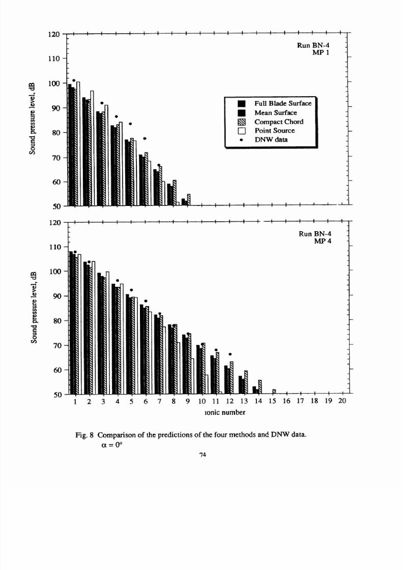
8/10/2019 NASA ANOP Propellers
http://slidepdf.com/reader/full/nasa-anop-propellers 80/104
120 I I I I I I I I I I I I I I I I I I I I
Run BN-4
MP 1
110 -
Orl • Full Blade Surface
90 mlWlml. [] Me.,
Sue.:e
I_llill I_1 lffl *
[] Compact
Chord -[
80-[l[lll[IEll[I
[]
Point Source ]-
•
• DNW
data
i
70
60
50
o
o
0
c_
120
110
100
90
80
70
60
50
Run BN-4
MP4
1
2 3 4 5 6 7 8 9
10
11 12 13 14 15 16 17 18 19 20
ionic number
Fig.
8 Comparison of the predictions of the four
methods
and DNW data.
ot=O °
74

8/10/2019 NASA ANOP Propellers
http://slidepdf.com/reader/full/nasa-anop-propellers 81/104
t_
>
tD
r_
rA_
0
120
110 I •
100
90
80
70
f
[
f I I f I _ t
[ J I I [ t
• Full Blade Surface
i Mean Surface
[] Compact Chord
[] Point Source
• DNW data
[ [
I
F
Run GN-3 l
MP 1
6O
50
120
110
m 100
;>
-
90
80
n_
o
70
6O
50
1 2 3 4 5 6 7 8 9 10 11 12 13 14 15 16 17
Harmonic number
Fig. 9 Comparison of the predictions of the four methods and DNW data.
ot = -7.4 °
75
18 19 20

8/10/2019 NASA ANOP Propellers
http://slidepdf.com/reader/full/nasa-anop-propellers 82/104
_a
O_
"0
o
r_
12°
10
100
9O
8O
7O
6O
I
F t
I I
I I I
I
I
I
I I t I I
t
I I
I
Run EN-2MP1 1
•
Full Blade Method
1
Mean Surface
[]
Compact Chord
[]
Point Source
•
DNW data
e_
o
r_
5O
120
110
100
9O
80
70
6O
50
2
3
4 5 6 7 8 9 10 11 12 13 14 15 16
Harmomc
number
Run EN-2
MP4
17 18 19 2O
Fig. 10
Comparison of the predictions of the four methods and DNW data.
ct = 7.3 °
76
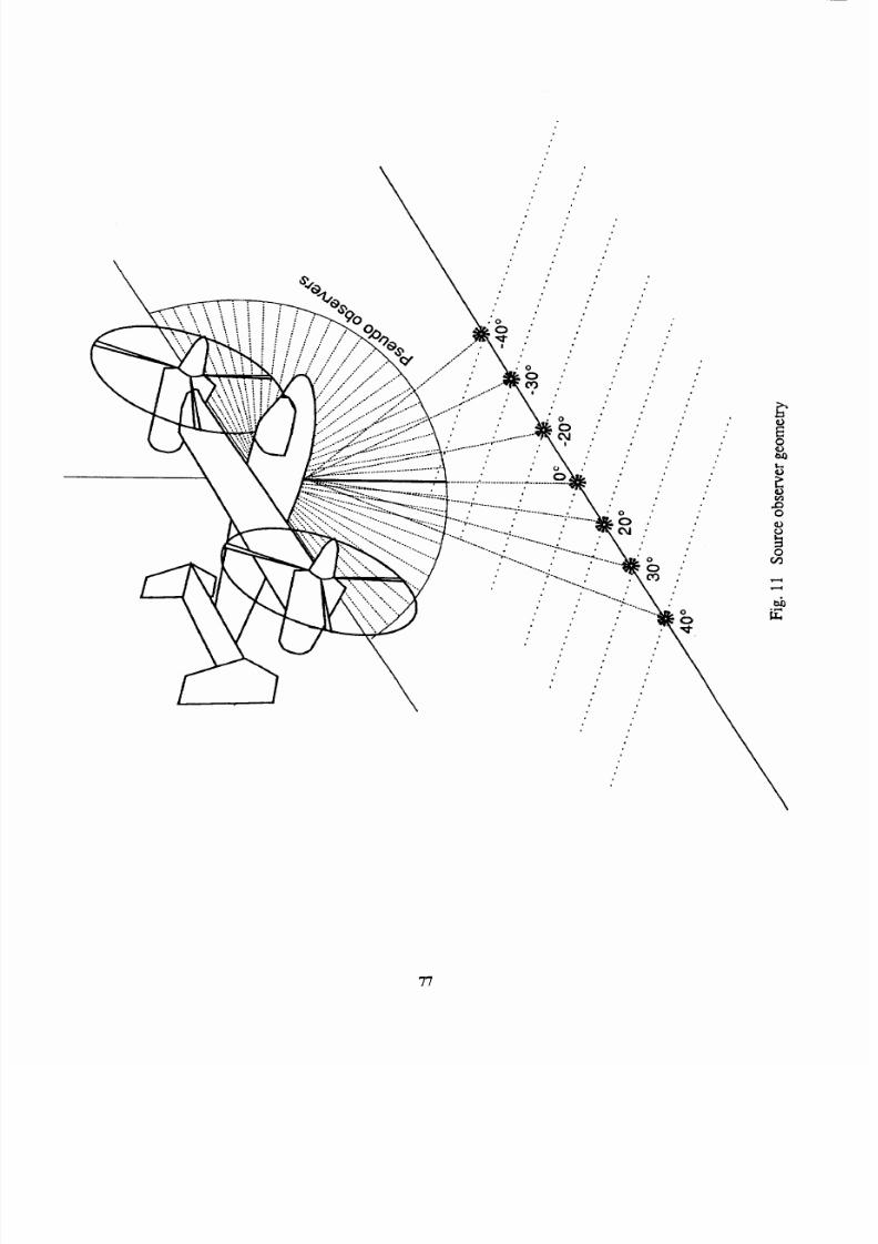
8/10/2019 NASA ANOP Propellers
http://slidepdf.com/reader/full/nasa-anop-propellers 83/104
0
0
0
, S
•
.
0
° •
0
• °
• °
0'
°
0"
°°
*
°°
°°
°°
°"
°°
o°
°°
o°
77
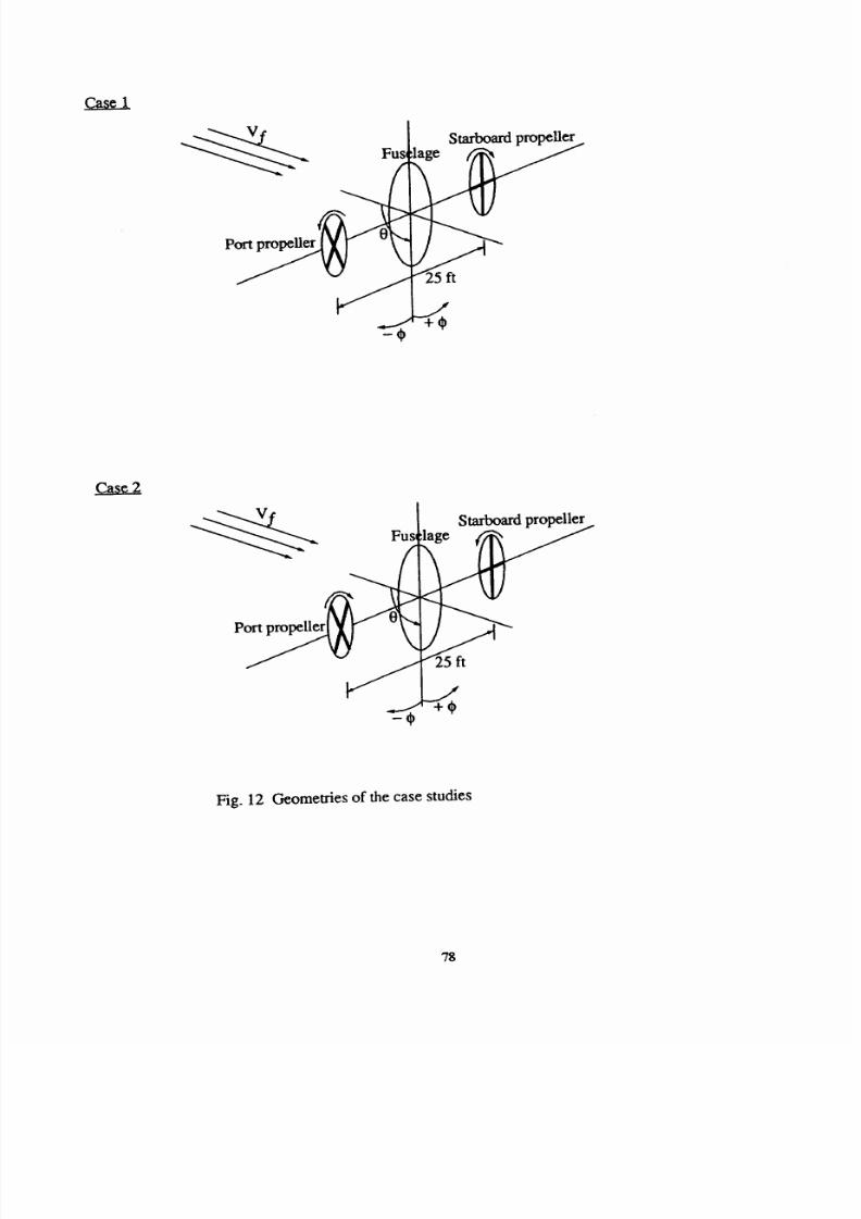
8/10/2019 NASA ANOP Propellers
http://slidepdf.com/reader/full/nasa-anop-propellers 84/104
Starboard propeUer
"__ _25 ft
Fus,
Port pro_
-%
Starboard propeller
lage
Fig.
12
Geometries of the case studies
78

8/10/2019 NASA ANOP Propellers
http://slidepdf.com/reader/full/nasa-anop-propellers 85/104
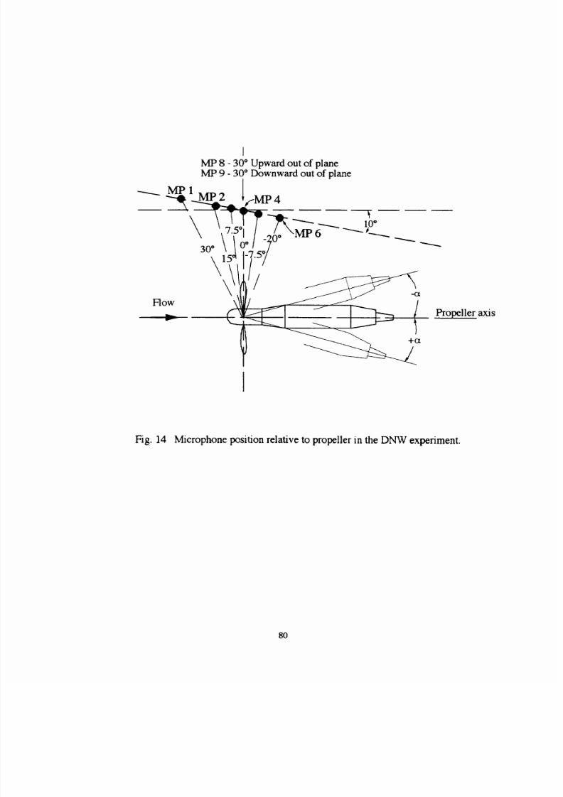
8/10/2019 NASA ANOP Propellers
http://slidepdf.com/reader/full/nasa-anop-propellers 86/104
Flow
I
MP 8 - 30* Upward out of plane
MP 9 - 30* Downward out of plane
"_1 MP2 ,lfMP4
v
;./-_0 _
\15,1 1-_/.5_
\_ Id
/
_ Propeller
Fig. 14 Microphone position relative to propeller in the DNW experiment.
80

8/10/2019 NASA ANOP Propellers
http://slidepdf.com/reader/full/nasa-anop-propellers 87/104
120 ......................
CN-3 i
L
110 ';-
10o
k o
9OP
E
80
L
7o
60 i
,
O
O
o
a= o ° MP2
2
d
-i
o J
J
120
110
100
90:
8O
7O
60
A_
I I ; I I I I ; t 1 I I ; I I I I _ I
CN-3
a = 0 ° MP 4
)
I
PAS
O DNW
O
0 0
' t
'
I I I L : t I I I ,
120_ .................. -_-_-=
q
ct = -3.6 ° FN-4
110 _ MP2
_- P
aa 100 ":-
>
b
90
O1
[
"_ 80
O
7O
60
O
©
O
-q
-I
4
--4
O
-I
o
d
o q
5
-4,'
I _ I L 1 t ; i 1 i i i I I ;
120 i ..... _-'-_-_'--_--_'-_---'--_--_-_--_--'--_-"
L
110 F-
F
100_ o
k
1-
90.:-
80)
L
70 _-.
60 I,
O
O
O
(x = -3.6 ° FN-4 _
MP 4 -4,'
7
4
o
, I I I I I [ i I I i I I I _
120
110
100
9O
80
7O
6O
I I I ; I I I I ; t z i r ; I I I i ;
a = 7.4 ° GN-4
MP 2
1
O
3
5 7 9 11 13 15 17 19
120 r_--r ,---_-_--T- ..... _-,---_--_--_---_--,---_-_
k
110
L
loo
E
90_
i--i
80_
l--i
70_
6oi
=
7.4°
GN-4
MP4 i
4
4
-M
: l I I i ', 1 r I I = I I ,
1 3 5 7 9 11 13 15 17 19
Harmonic number Harmonic number
Fig. 15 Comparison of PAS prediction with DNW data at MP2 and MP4 for the round tip propeller.
Q = 1800 RPM
81

8/10/2019 NASA ANOP Propellers
http://slidepdf.com/reader/full/nasa-anop-propellers 88/104
120, ....................
,_ BN-4
110
L
_.,-_)
U.
100L-
'-'
b
F
9O_
g.
70
F
k
60 .
O
O
Or= 0 °
MP2 -'
-q
)
(1)
-'-4
ll0L
@
I--I
_-I C)
100
9O
80-
70,-
*.--I
60 ""
120
_ ....................
..
(x =
0 ° BN-4
MP4
@ ,
I PAS -q
o
o
DNW ]
® j
(
i o o 4
, I I i t I l ' a--_ _'*
120:, , , , , :
, , ,
. ,
,
_--_--_-_------_-_--
f --,
110
,._ _,
"_ 100 _ o
=
9O_
"
--i
80.,
t
70,-,
60-1
)
O
O
¢.--_
_'_ O
a
=
-3.6 ° FN- 1 -
MP2
±
--4
O
-4
o
i
1 i I
i
_
: i
I_
120
,--,-
-_--,--_--,-_
,
,
, ,
, _
, ,
,-_--,---_-_
FN-I i
110
b
100
90_-
sol:
F
F
70 L
60 i ,
c_
=
-3.6 °
MP4 __
4
0 -.
©
Q
@
4
t
q
lilll_ll
120 ....................
110
100
90
8O
7O
60
ct = 7.4 ° GN- 1
MP2
O
O
9
I
O
O o
I
120.-_=-,--,--_--_ , , _ _ ,
,
, _ , , , ,
,
,:
c_
=
7.4 ° GN-1 -_
110 _ MP4_
4
,:_ -i
100_
_
i 4
,_ i ®O 4
90L
i.-
F c_
L.
80_ _.
F 0
F
70 -
2
60 _
1 3 5 7 9 II 13 15 17 19 I 3 5 7 9 II 13 15 17 19
Harmonic number Harmonic number
]zig.16 Comparison ofpredictionwith DNW dataatMP 2 and MP 4 fortheround tippropeller.
= 2100 RPM
82
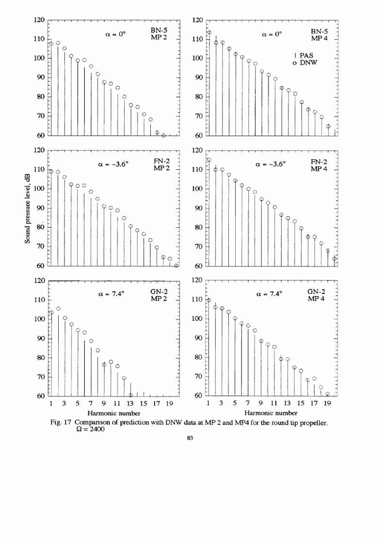
8/10/2019 NASA ANOP Propellers
http://slidepdf.com/reader/full/nasa-anop-propellers 89/104
0 -__ o
11o L
t
80
7O
o
_oo
()
o
Oo
o
o
MP 2
d
-4
d
o
o
120 ,:...................
r-
llOi- cG._
i--
L
100_
+_
90-
80 P-
k
7o
60:;
(
(D
(P
c)
o
...4 I
__-0
°
©o
o
(_1 ()
BN-5 +.
-i
MP4 :
-i
I PAS i
DNW
o i
---4
IlT
120 ................ -_--_-_:
:;_ +++
L
110
_o
I:I::1 i-+
_100_
= 90-
k--i
C_
t'u +_
O +.-+
70_
;-I
C.)
)oo
ct = -3.6 °
O
O
'-'O
I o
Ii
FN-2 i
MP2
2::
d
"1
---I
-]
o
o
Id
120 _-==--,--, .......
. a = -3.6 °
110 _ ,_"©
•-, @
+' (+1)
100_ ©
_, O
,-.j
()
90_ O
+--I
80_
+--I
I-i
+.-I
70_
,-I
60
@
©
.J
FN-2 i
MP4
--.q,
.-1
O "
l,i-+
120
11o
lO0
9O
80
70
<.3
60 i
1
I I I ; 1 I I I ; I I I ; I I I t
= 7.4 ° GN-2
MP2
o
o
o 0
3 5
o
o
(DOoI) _
7 9 11 13 15 17 19
Harmonic number
120 ; ......... - ........... :
¢x = 7.4 ° GN-2
MP 4 -
110_
-, _ )
+--I
100
,--I
,..-I
_-I
_-I
;-I
80 _4
LI
_-I
:--I
70-+
,--i
,--I
+--I
60 ''
1 3
o
Q
_a_ 0
o
@
o
I
)
0
t
d
-t
-]
-i
Q
1°
5 7 9 11 13 15 17 19
Harmonic number
Fig. 17 Comparison of prediction with DNW data at MP 2 and MP4 for the round tip propeller.
f2 = 2400
83
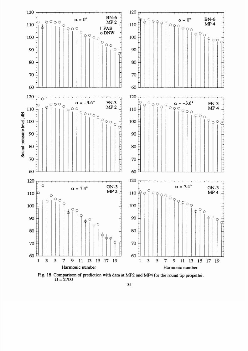
8/10/2019 NASA ANOP Propellers
http://slidepdf.com/reader/full/nasa-anop-propellers 90/104
120, .................... j
o BN-6 _
0_=0
,'_ 0000
110 _ ¢
F
L
100 :_
9oh
L
mF
F
70
L
60 _ ,
0
O00
O
OO
MP2 -,
I
PAS
o DNW -
o o q
0 "1
O0 4
o4
4_
4
J
4
4
J
120 L.................... "
.,ki) O
110
lOO
b
90_
F
70
b
k
60 L_____ ..... ... .
Gt=O
°
0 0 0
© 0 0
BN-6
MP4
¢O O
r_o o c_
"4
120 .................... 120
r o o 3 a = -3.6 ° FN-3 "
110
o 100 :'-
90,':-
O
r/_ L
70 '_
F
60 i.
0
)OO
0 0 0,.,
"0
4
MP 2 _i...'
q
4
00 0
0 -'
"I
4
"i
4
"-
I
110
100
9O
8O
7O
60
0
C) 0
0 o
a =
-3.6 ° FN-3 -,
ooo MP4
A
00 '0 -_
O00 ..,
f-)
120 ..........
110
100
9O
80
7O
60
0
0 o
,9
0
i i i ; i i i i
a = 7.4 ° ON-3
MP 2
O
(I)
Oo
O
(1)
¢
(D_
120 ,T--_,--_-_-_--_
........
_-_--_----_,
-i
,_ _ = 7.4° ON-3
110_¢°Oo_, MP4
--i _J O
"" 0 4
100_ °o 4
'-' (DO0 .4
"
90 ..T., 0
:,.-_
_-i '0_
"-'
80 _ -_
4
I I i
I
, 60 rl _ i ,
1 3 5
7
9 11 13 15 17 19 1 3 5
7
9 11 13 15 17 19
Harmonic number Harmonic number
Fig. 18 Comparison of prediction with data at MP2 and MP4 for the round tip propeller.
f_ = 2700
84

8/10/2019 NASA ANOP Propellers
http://slidepdf.com/reader/full/nasa-anop-propellers 91/104

8/10/2019 NASA ANOP Propellers
http://slidepdf.com/reader/full/nasa-anop-propellers 92/104
120
110
100
90
8O
-i
-i
-I
,..,-n
,,-I
I-.-]
I
I
I
70
z,,-t t
F_
L' t
6o_i ,
a = -3.6 ° FN-1
MP6
I
.k
[, o
d
J
--d
d
--i
i
J,l ,i _
110
120 : ....................
L GN-1
a = 7.4 °
_- MP6
-
lO0
90
8O
7O
6O
)
}
_}
,_>
I
PAS _:
o DNW -i
-4
k
110
100-
- __
=90,'.:-
° t
-
70 _ I
i,
60i, _
ot
= -3.6 °
FN-1
MP 8
t
I
I
II•
,
[
i
I
I T
I
I
:
120,
,
r---_--_-_-, ............ .;
F c_
=
7.4
°
GN- 1
- sa,8
II0 )
;r
_.
,_'.T, -
100 _
':';
_ d
90- _ -_
70
E_
I f
-_
120
110
100
9O
8O
7O
6O
I l I i n
r
I I ; r I T_T T r I P _ ;
et = -3.6 ° FN-1
MP9
0
0
I
i
I
i
3 5
(D
, [ I i
illll
7 9 11 13 15 17 19
Harmonic number
120 ry ................. _-_-__,
F
110
100
9O
°
70
6O
1
_
c9
a=7.4 °
GN-1
MP9 _.
4
0 4
, I I : I I i I I i
5 7 9 l l 13 15 17 19
Harmonic number
Fig. 20 Comparison of prediction with DNW data at MP6, MP8 and MP9
for the round tip propeller, fZ = 2100 RPM
86
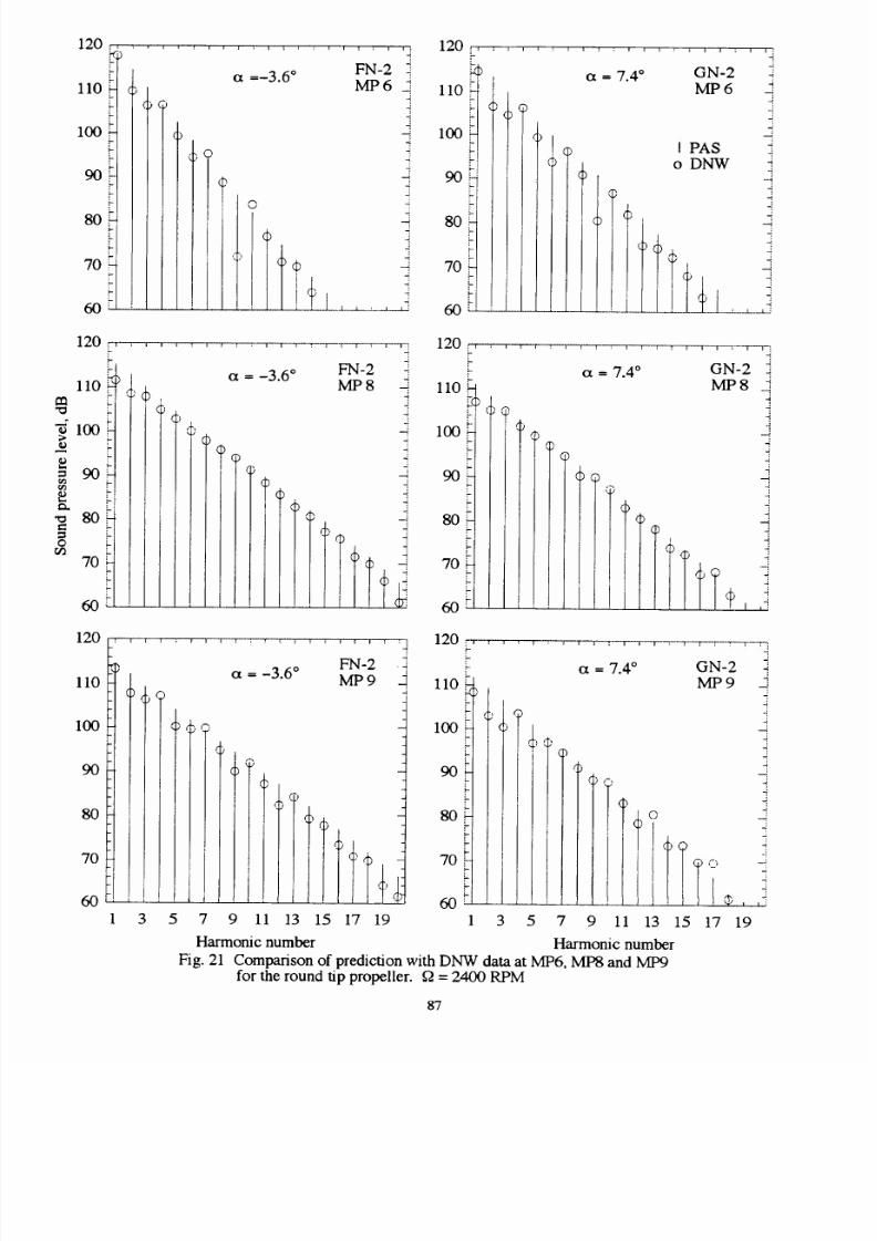
8/10/2019 NASA ANOP Propellers
http://slidepdf.com/reader/full/nasa-anop-propellers 93/104
F
llOL ¢
100_
120 ....................
FN-2 i
90
80-
70-
I
(0
O0
_,O
, ¢',
a =-3.6 °
©
0 L,
_6_
q
-i
-.4
? i
'I_,
'4) 1
120
110
100
9O
8O
l
t
7O
60
;Itl:llZill_tlll,ll;
@
"'[¢
¢
i,
I
ct =
7.4
°
+
i
GN-2 i
MP 6 -,
I PAS -'
o
DNW -'
120
:.,.
................... j
FN2 -
a
=
-3.6 ° - "
110_ _
100_
>
=90-
_ L
_
L
_
==
80)
O t
r,_
L
70 ';-
v0
¢) .
¢
fl)
(
q)
q)
(1)
{
MP8
S
-I
-4
......4
.4
tTti
120 _ ......
P
110 _
100-
90
80
7O
6O
a = 7.4 °
,¢
(
@
¢ ,
I
Ii,
I
GN-2
MP8
,q
--.4
J
)
lift,
J i , I
120 • _ .... ... ... ... .. ... .
110 _-
v-
100,-
90,-
v-
v-
l=-
I--'
80_
FI
i-i
70_
1
,©
FN-2
ct = -3.6 ° MP 9
;
©
q0
(1)
(D
, i i i
J
1 , I , , )
5 7 9 11 13 15 17 19
Harmonic number
120
110
100
: I _ I ; _ I I : I ""l I _ r I I _ I'--T-{
.
_x =
7.4 °
GN-2 -.:
<)L MP9
,©
-4
90 '
.q
I I
60 . ' _ , I I . . ¢, ,q
1 3 5 7 9 11 13 15 17 19
Harmonic number
Fig. 21 Comparison of prediction with DNW data at MP6, MP8 and M1x)
for the round tip propeller, fa = 2400 RPM
87
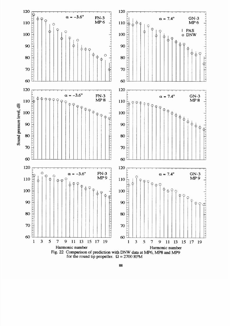
8/10/2019 NASA ANOP Propellers
http://slidepdf.com/reader/full/nasa-anop-propellers 94/104
120, .. ... ... .. ..
L
110
F
100 F
F
g
9O,"-
L
70 F
6OL
)
0
f
©
ct =
-3.6
°
©
O
03
..I_¢ o
4
MP6q
q
q
q
4
i
q
¢ 4
120 ................
110
100
90
8O
7O
6O
©
O
4
ct = 7.4 ° GN-3
q
MP6 -.
..
o I PAS ":
_)
._
o DNW -:.
i "_ -q
i •
o -
i (1) .2:
i
1
120 , ......... _--_--_ ',', , ,j
_ ct
=
-3.6 ° FN-3
110:,_¢
,cD )©o
_c_ MP8
4
>° 100-_ ¢o¢ -_
90-
t_
0,, :
0 __
_ L
70 _-
60 L
120 _,
,t_
110 _ ¢ • ¢ :_,¢,
_..
100 ::-
80-
L
70 _-
P
b
F
60 _,
_t
=
7.4 ° GN-3
MP8 q
"4
OM() i
¢®
i (D® ._
4
I ,
120
110
100
9O
8O
7O
60
i
[-I
_4
1
(D
o FN-3
o o MP9
(D (I)@
t
3 5 7
ct = -3.6 °
O
,a., (I)
r-_
( _ ,q.,
I
I
'
I
i
I
I
(0
÷
I
I
I
I
9 11 13 15 17 19
Harmonic number
120 [-_-----,--,-,
o
110 _
,-, )©
e/
100_
,..-i
90_
i--i
8oN
w-I
70-.
®i
1 3 5
1 r
:
i i
1
_ i I--I' r I I
:
ct
=
7.4 ° GN-3 ___
-4
MP9 __
¢_)0o
0 -
i
7 9 11 13 15 17 19
Harmonic number
Fig. 22 Comparison of prediction with DNW data at MP6, MP8 and MP9
for the round tip propeller. _ = 2700 RPM
88

8/10/2019 NASA ANOP Propellers
http://slidepdf.com/reader/full/nasa-anop-propellers 95/104
120
110
100
9O
8O
7O
6O
.qq)
a = 0 ° CC-3 ._
MP2_
o
O
o
O
q
A
O -1..
O
, 1,9., ,, _,,,.,, _
120 :, ,
110 _-
k
100 i
90 -
8oj
i
70
i J
6o
O
a=O °
0
I PAS
o DNW
IL
o
CC-3
MP4 _
-4
--4
I I :
120 f., .. .. ... ... ... .. ... .
ct = 3.8 ° LC-4 -
110
_a 100_
90
r_
r_
-_ 80
70
60
o
o
O
O
i T II l
MP 2
2,,
-I
-I
4
I I :
L_
110
___
100 _ 0
90_
i-
80.::-
k
7O
O
o
c1 = 3.8
°
LC-4
MP4_
4
-1
"--I
4
_j
O
I
_l_lllilLi,i
I :
120
110
100
9O
8O
70
6O
I
I I ;
I I
i
I i 1 I
I
l _ t I I I
a
= -7.3
°
EC-4
MP2
-o
o
O
o
©
1 3 5
o
o
o
o
7 9 11 13 15 17 19
Harmonic number
120_ .......... _.., ,
L
_- (x =
-7.3
°
110 _
100_ i ° °
90 , o
i-
0
80 o
70 I o
C,
60 ] ] o , ,
1 3
EC-4 _
MP4 3
-4
-4
4
I _ I i I
I
i
5 7 9 l l 13 15 17 19
Harmonic number
Fig. 23 Comparison of prediction with
data
at MP2 and MP4 for the square tip propeller.
Q = 1800
89

8/10/2019 NASA ANOP Propellers
http://slidepdf.com/reader/full/nasa-anop-propellers 96/104
a = 0 ° BC-4
MP2
110
7"
b--
o
9O
80-
L
b
70
1.
60 I ,
100
0
0
1
i
o
o
o
o
I°°
I
o
1
.4
-4
d
q
q
tililillJ
110 _ MP4 _.
bl
100 >
b
9OP
L
8O-
b-
70
k
6o_
p
Q o I PAS
o o DNW
©
I
i
o
o
o
o
Oo
.i
q
--4
"i
--i
3.8° Lc-1
110_
F
100 ::-
90-
b
7O
60-,
©
O
0
o
o
o
o
i
O
4
4
-4"
4
A
I
i
I
I _ :
I
I i
120 r_=---_---_--_--'---_---r--_-_.--_--_--_---_-'-,--_--r--=--r--_
a= 3.8 ° LC-1
L
MP4_
'0
o
i
1
I
i
i
i
J
o
o
o
I
o
o
110 [-
-t ¢-,
1t30.--,
--I
90
80
70 _
q
4
d
-i
4
-q
d
I i I I i ' 1 I i
120 _ ................
-r--r--
c_
=
-7.3 ° EC-1
MP2
110
100
90
80
7O
O
O
-I
1
6O
Q
O
f't
"_O
O
Q
0
Oo
O
O
3 5 7 9 11 13 15 17 19
Harmonic number
120 _TT---'r-- T'----r-- i i r
I i
1
;
-_i_--_-.
b- -:
110 -
o
_..
10o
9O_-
b
8o
k
_._
7O
60
1 3
<x
=
-7.3°
EC-1
MP4.
i
0
©
o
o
o
o
O
0
I
I
5 7
d
-4
d
4
9 11 13 15 17 19
Harmonic number
Fig. 24 Comparison of prediction with data at MP2 and MP4 for the square tip propeller.
= 2100
90
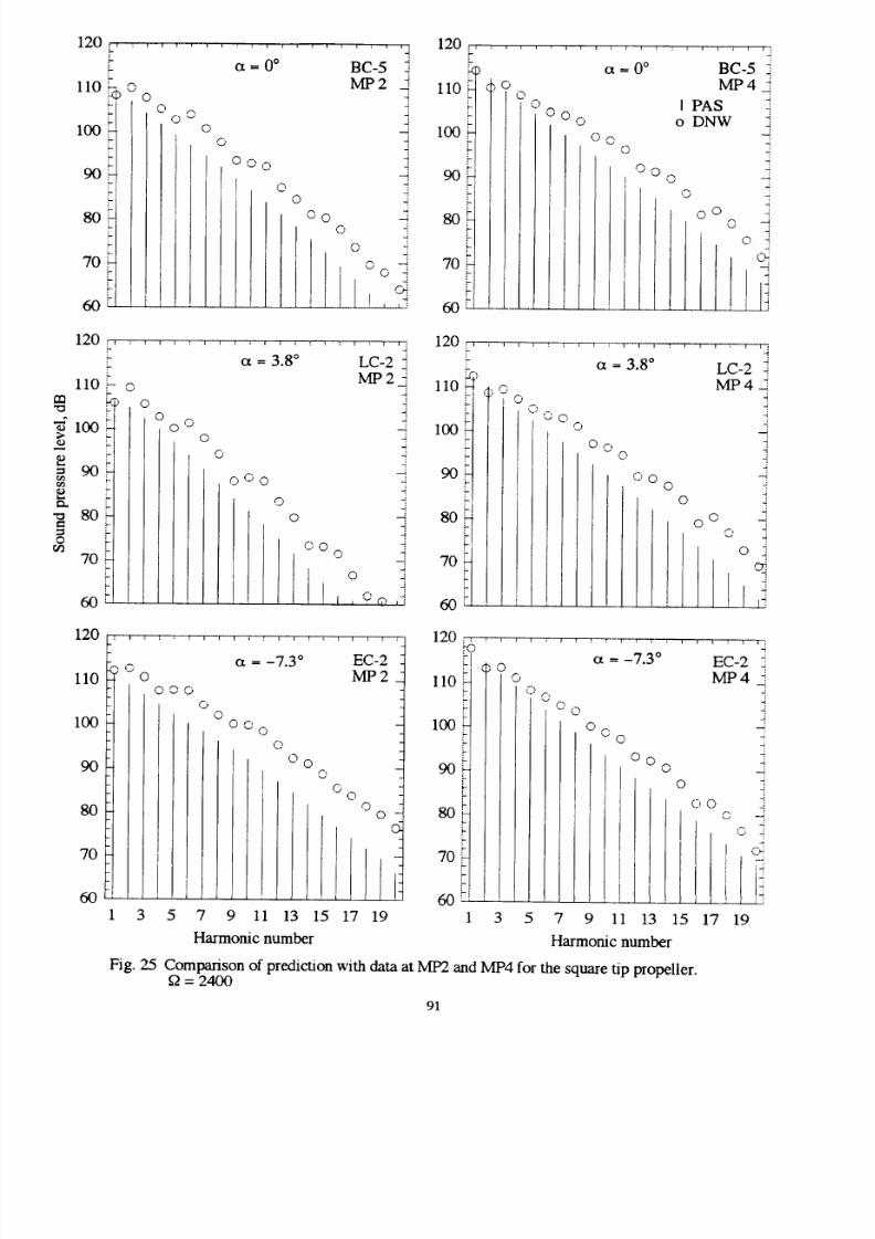
8/10/2019 NASA ANOP Propellers
http://slidepdf.com/reader/full/nasa-anop-propellers 97/104
120 .....................
-
t
llOto
t
8o
'2-
7o
60 t ,
0
0
0 o
I
i
I
0
0
ot=O °
BC-5 -
MP2
O0 o
I 0
0
I'10000,
-1
-I
i
I, ,i
120 _...................
110_ cno
t 0
L
100
_..
90_
L
80.:-
t
70
0 _ i
)0 o
00
0
00:,
LJ
i
I'
ct=O °
I PAS
o DNW
I ;
BC-5
MP4_
q
0
oO i
120
110
"_ 100
=
90
r.e2
O
m 70
60 .
;lll_lli;lll l-"l'l;[yq
O
0 o
0
0
0
o
c_ = 3.8 °
000
0
Ili
I o
d
LC-2 2,,:
4
d
-4
5
--3.
"I
©
o
,L_4}
110 _ _ o
©
i..-i
100
u-i
90--,
;--i
80,-,
70_
60 ''
120 _ ..... _-_--.-_ ...... T-T-- ,TT'-]
c_ = 3.8 ° LC-2 i
MP4£;
fi
0 0
0
o 4
000
0
0 0 q
0 q
I
I
i
i
I
i ,
0
, I",,"
120
110
100
90
8O
70
6O
0
O
OOO
I 1 I
;
I I I 1 _ _ I I 1 _ I I I I ;
ct = -7.3 ° EC2
MP2
0
0
d
O0 o
0
°o
0
©
iioo
9 11 13 15 17 19
120 _ ........ --,--, .......
110
100
9O
80
70
,<)
,_ 0
, 0 0
' 60
1 3 5 7 1 3 5
Harmonic number
d
ct - -7.3 ° EC-2
MP4_
-4
C) 0
0 _
0
I ©0
o
0 _
0 0
"I
0 '
I
7 9 11 13 15 17 19
Harmonic number
Fig. 25 Comparison of prediction with data at MP2 and MP4 for the square tip propeller.
f_ = 2400
91

8/10/2019 NASA ANOP Propellers
http://slidepdf.com/reader/full/nasa-anop-propellers 98/104
130 - .................... q
ot
=
0 ° BC-6 q
MP2]
-q
O
O Oo
L
120 i- o
110 '
i
0
80
70
0000
Q
I PAS
o DNW
©O o
0 0 0 0
130: .................... j
a
=
0
°
BC-6 -
t-
120
h
110 _
100 _
r
,2
80_
L
70 _,
00000
' I
, I
1
O00
oO o
±
000
MP4_
O00
-i
I
L
120_
o
"d 110 :.L
100
•_ 90
0
m 80
70
000
c_
=
3,8 °
0
000
0
0 o
O0
LC-3
000 fi
0
?
130 ._--,-_-,--_-=-_--_,
c_ = 3.8 °
120 _
0 () 0 O 0
llO F
9o) ,
I
L _
70 _, I
000000
LC-3 ]'
MP4 q
0 () 0 ]
0 O 0
c_
]
i
q
130
120
110
100
9O
80
7O
:
I I I
•
I I I I _ _ I
I ;
;
T I
I I
ot
=
-7.3
°
EC-3
Oo
MP2
-0
0 o
0 OOO0
0
0 -
1 3
] I
I
_ [
5 7 9 11 13 15 17 19
Harmonic
number
130,, :
,
I--T--'7"--'FrrTT I , _ , I 1 r I
h _
=
-7.3° EC-3
MP4
120
c ,
o o o c o 0 0 o
0 () 0
i
110
100
9O
8O
7O
1
O0 o
0
0 0
t I
3 5 7 9 11 13 15 17 19
Harmonic number
Fig. 26 Comparison of prediction with data at MP2 and MP4 for the square tip propeller.
f_ = 2700
-4
92

8/10/2019 NASA ANOP Propellers
http://slidepdf.com/reader/full/nasa-anop-propellers 99/104
120, ....................
_ MP6q
10_-
100'
k
80
70
60
o
)
©
i
©
O
--4
,
II:lll]lll'll:
120
_....................
i a
=-7.3
° EC-4
110 _ MP6j
h
Q
100 -
C)
90
0 o
80
I1
60 • |*
I PAS
o DNW
J _J___I--L--..d----.L_ I
-q
I ' I I ;
120 , ...................
E
110 P
m ::
100_
k
_ 90
"_ 80
o
m 70
6O
©
©
©
J ©
a
=
3.8 ° LC-4 -,
MP8 -
.-I
-t
.-t
0 _
, I ....... , .... i
120 ,_-, ............
b ot = -7.3 °
110 _
100 _
,3
O
9oE o
©
80
0
70
60 ,
EC-4
_
-4
q
----t
4
.q
i
I l ] i I I i : I t i
120 ....................
cx = 3.8 ° LC-4
110
100
9O
8O
7O
6O
O
©
1 3
()
MP9
v
©
©
I I I ' i _
I
I _ 1 I I I I
5 7 9 11 13 15 17 19
Harmonic number
110 ._
100 _
9O
80
70
60
1
0
(i)
'4
et = -7.3 ° EC-4
j
q
A
4
o i
G 4
4
5 7 9 11 13 15 17 19
Harmomc number
Fig. 27 Comparison of prediction with DNW data at MP6, MP8 and MiX)
for the square tip propeller, f_ = 1800 RPM
93
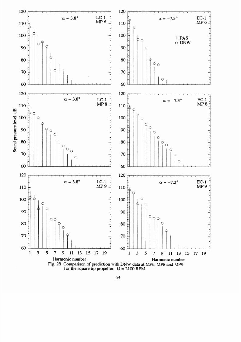
8/10/2019 NASA ANOP Propellers
http://slidepdf.com/reader/full/nasa-anop-propellers 100/104
110
100_
90-
80-_
70_
60 ,.
120 : ....................
,- -i
ct=38 ° LC 1
MP6_
]
o
I
tl
q
12oF
................... i
r a = -7 3 ° EC-1
-_
MP6_:
--1
110
1-
100 i-"
b J (I) 0
F
[
80_
L
70 _
r
60 L ....
Oo
I PAS
o DNW
q
--I
F
I ¢ i 1 I ,i
: L
I :
120
:
...................
k
L
L
110 _-
"_ _o
_ 100_
VI I"1
_ ,.-i
70_
o
)
} 0
0
0
o
'q
ot = 3.8 ° LC-1
MP8 __
4
4
---4
4
0
© - ,
, I
I
i I I I I I
I
120 ;_
110_
k
b
90_
k
k
L
70P
i_
60 i ,
i r r -I ;l
= -7.3 °
(D
o
_j
o
o
o
o
-1-- I l ; I _ i
"
EC-1 Z::
MP8q
4
o
....-4
o
120
110
100
9O
8O
7O
6O
I I 1 i i I I 1 i I 1 I -[ 1 I I i "-7
ct
= 3.8 °
LC-1
MP 9
3
0
@o
I
II
I
0
IIl:l
120 ..... - .... --, ....
c_
=-7.3
°
EC-1
110
0
i-
_
100 _-
90a
i-
8o _
70 ) :
k
6O_. i
1 3
0
0
T (
0
I
5 7 9 11 13 15 17 19 5 7
Harmonic number Harmonic number
Fig. 28 Comparison of prediction with DNW data at MP6, MP8 and MP9
for the square tip propeller,
g2
= 2100 RPM
MP9£:
4
4
4
I
O
4
-
1
' I I I i 1 t i
9 11 13 15 17 19
94

8/10/2019 NASA ANOP Propellers
http://slidepdf.com/reader/full/nasa-anop-propellers 101/104
120 _....................
L
110_
loo#
F
80
L
70/
F_
60:,
®9
'<b
0
(D
()
ot
=
3.8
°
0
O
I
I
i
LC-2
MP6_
-4
i
i
l °°
, <_ ,_
120 ,o ....................
::: a
=
-7.3 ° EC-2
(_I)
110 _-
F
P
,a
100 _
F
8o _
F
70 ';-
F
i-
@0
@
__i
©
0
I
I i
MP6
I PAS
o DNW
-i
, i
LL
120
..........
110 _ ._ ©
I:rl [ O0 0
Q
100 ..-,
-i
90'-"
[..9
.'u 80
o
7O
6O
-i
-i
-i
-i
-i
-i
-, l
O0
i i , I ---r--'T---Z--T--'T 7
=
3.8 ° LC-2 _
0
0
O
0
0
0 o
_ d
I 4
'li , ,
1
.It z-v ,r'T---r--. -r _ _ _ _ _ _ :
, ,
: _ r ---r---q---T---r--
}-
., (_©
110 '_
I'-I
80 _
:1 ,
1
70 _
60 FI .
0
Q
0
I
0
0
c_
=
-7.3 ° EC-2
MP8
0
O
0
0
0
0
0
©
0
0 0
120
110
100
9O
8O
7O
6O
i i i _ i i i ;
i
T ( _ 1
i
i ; i
i
i
ot
=
3.8 ° LC-2
MP 9
@
©
@
1 3
_0 o
I
I
O
0
0
O
0
O0
ii iOo
5 7 9 11 13 15 17 19
Harmonic number
120 i
.......... -,-., ........ ,
t ° i
c_
=-7.3
° EC-2
110 i
90
80
70
6O
1
MP9
d
I
'1
iI
5 7 9 11 13 15 17 19
Harmonic number
Fig. 29 Comparison of prediction with DlX_ data at MP6, MP8 and MP9
for the square tip propeller, g2 = 2400 RPM
95

8/10/2019 NASA ANOP Propellers
http://slidepdf.com/reader/full/nasa-anop-propellers 102/104
120
o 110
>
= 100
rll
e_
•_ 90
o
80
130 ...................
a
= 3.8 ° LC-3
120 MP 6
110 o
O
i
100
, ¢ Ooo
z"-,
C-' 0
9O I
I 0
I
8o I
I
i ,I
2
70 ' --'-
130 ....................
a = 3.8 ° LC-3
MP8
70
130
120
110
100
9O
80
70
o00OOOOo
O0
I
0 0 C,
I
I
I
I
---_
fm
"_0
0
0
I
r
I
]
I
I
_ _ .- -- .4,'
cx = 3.8" LC-3
MP9
)_
0
OoOo00
O000
0 o
0
"_C
3
I
I
I
5 7 9 11 13 15 17 19
Harmonic number
130 ....................
a
= -7.3 ° EC-3
MP6
120
(1) _ 6)
110
100
90
80
0 -_--
c}
© O
¢,
,::J)
i
I PAS
o DNW
130 ....................
k
a
= -7.3 °
120
P
[ ¢ Q(:'O 000 O Oo
t ) 0 o
llOI °o
[
t
lOO[
t
9ol
' I
+of
t I
70 t .....
A
......... ,....
130 .........
EC-3 i
MP8
1
O
O O
OC
I
1
1
120 o
0
110
i
i
100
90
80
70
1 3
a = -7.3 °
0
C;, 0 0 0 '0
'0 0
IIJ:lll,l
EC-3
MP 9
5
OO
O
O o
0
I
i
7 9 11 13 15 17 19
Harmonic number
Fig. 30 Comparison of prediction with DNW data at MP6, MP8 and MP9
for the square tip propeller, f_ = 2700 RPM
96

8/10/2019 NASA ANOP Propellers
http://slidepdf.com/reader/full/nasa-anop-propellers 103/104

8/10/2019 NASA ANOP Propellers
http://slidepdf.com/reader/full/nasa-anop-propellers 104/104
REPORT DOCUMENTATION PAGE
F or m A pp ro ve d
OMB No. 0704. 0188
Public reporting burden for this collectmn of 0ntormal_n is estm_amd to average 1 hour per response, mduding the "me for rewewmg instnx:lmnS, ma.rch,ng oxming data sources,
gallN_ircj a¢<l rn_ntanng
U_
data needed, and ¢ornp4ehng aP,¢l mvmvang
_
coiklchon of infofwlabon. ,Send oommen_ regardincj
this
b_rdqm eltima_ or any ott ler aspect of
this
o=41ecl_ of infom_bon, including suggestions f or mduang _ burden, to Washington Headquartlrs Servmes. Oimclorata for Infom ,a_on Operation= and Repocts. 1215 Jeflemon Daws
Highway.Suite;204. Arhngton,A 222O2-43O2,andto theOffmeof ManagementndBudgeLPaperwo_Reductx_Project0704-0188),Washmgt_,DC 205O3
1. AGENCY USE ONLY ( Leave blank) 12. REPORT DATE 3. REPORT TYPE AND DATES COVERED
J February 1997
4. TITLE ANDSU_/i/LE
A Users Guide
for
the NASA ANOPP
Propeller
Analysis System
6. AUTHOR(S)
L. Cathy Nguyen and Jeffrey J. Kelly
7. PERFORMING ORGANIZATION NAME(S) AND ADDRESS(ES)
Lockheed Martin Engineering and Sciences
Hampton, Virginia 23666
9. SPONSC_,:t G I
MONITORING
AGENCY NAME(S) AND ADDRESS(ES)
NASA Langley Research Center
Hampton, VA 23681-0001
11. SUPPLEMENTARY NOTES
Langley Technical Monitor: Robert A. Golub
Final Report
Contractor Report
5. FUNDING NUMBERS
NAS1-96014
538-03-13-01
8. PERFORMING ORGANIZATION
REPORT NUMBER
10. SPONSORING/MONITORING
AGENCY REPORT NUMBER
NASA CR-4768
12L OI, _I di UTION I AVAILABILITY STATEMENT
Unclassified/Unlimited
Subject Category 71
13. AI_._THACT l_xi mum 200 _.,,i_4)
121). DISTRIBUTION CODE
The purpose of thisreport is to document improvementsto the PropellerAnalysis System of the AircraftNoise Prediction
Program (PAS-ANOPP) and to serve as a users guide. An overviewof the functional modules and modificationsmade to the
PropellerANOPP systemare described. Propeller noisepredictionsare made byexecuting a sequence of functional
modules throughthe use ofANOPP controlstatements. The most commonly used ANOPP controlstatements are discussed
with
detailed
examples
demonstrating
the use ofeach controlstatement. Originally, the Propeller
Analysis
System included