autodock by anop singh ranawat
TRANSCRIPT

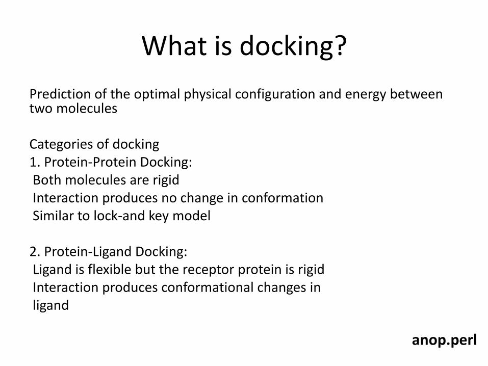
What is docking?
Prediction of the optimal physical configuration and energy between two molecules Categories of docking 1. Protein-Protein Docking: Both molecules are rigid Interaction produces no change in conformation Similar to lock-and key model 2. Protein-Ligand Docking: Ligand is flexible but the receptor protein is rigid Interaction produces conformational changes in ligand
anop.perl

AUTODOCK
• An Automated Docking Software for Predicting Optimal Protein-Ligand Interaction.
• Download from -: http://autodock.scripps.edu/downloads/autodock-4-2-x-installation-on-windows
AutoDock has applications in: • X-ray crystallography; • structure-based drug design; • lead optimization; • virtual screening (HTS); • combinatorial library design; • protein-protein docking; • chemical mechanism studies
anop.perl
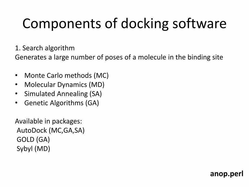
Components of docking software
1. Search algorithm Generates a large number of poses of a molecule in the binding site
• Monte Carlo methods (MC) • Molecular Dynamics (MD) • Simulated Annealing (SA) • Genetic Algorithms (GA)
Available in packages: AutoDock (MC,GA,SA) GOLD (GA) Sybyl (MD)
anop.perl
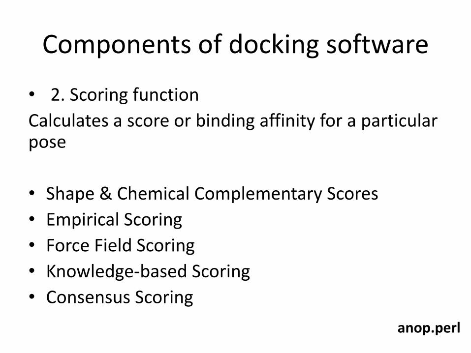
Components of docking software
• 2. Scoring function
Calculates a score or binding affinity for a particular pose
• Shape & Chemical Complementary Scores
• Empirical Scoring
• Force Field Scoring
• Knowledge-based Scoring
• Consensus Scoring
anop.perl
The Algorithms
anop.perl
Simulated Annealing
• Algorithm modeled after the cooling of a solution to form glass, though it’s better explained by crystal formation
• Given a long enough cooling time, molecules will relax into their lowest energy state to form the largest crystals
– Quick cooling - highly disordered system
– Slow cooling - highly ordered crystal, with each molecule in its lowest energy state
– Algorithm simulates either linear or proportional slow cooling
anop.perl
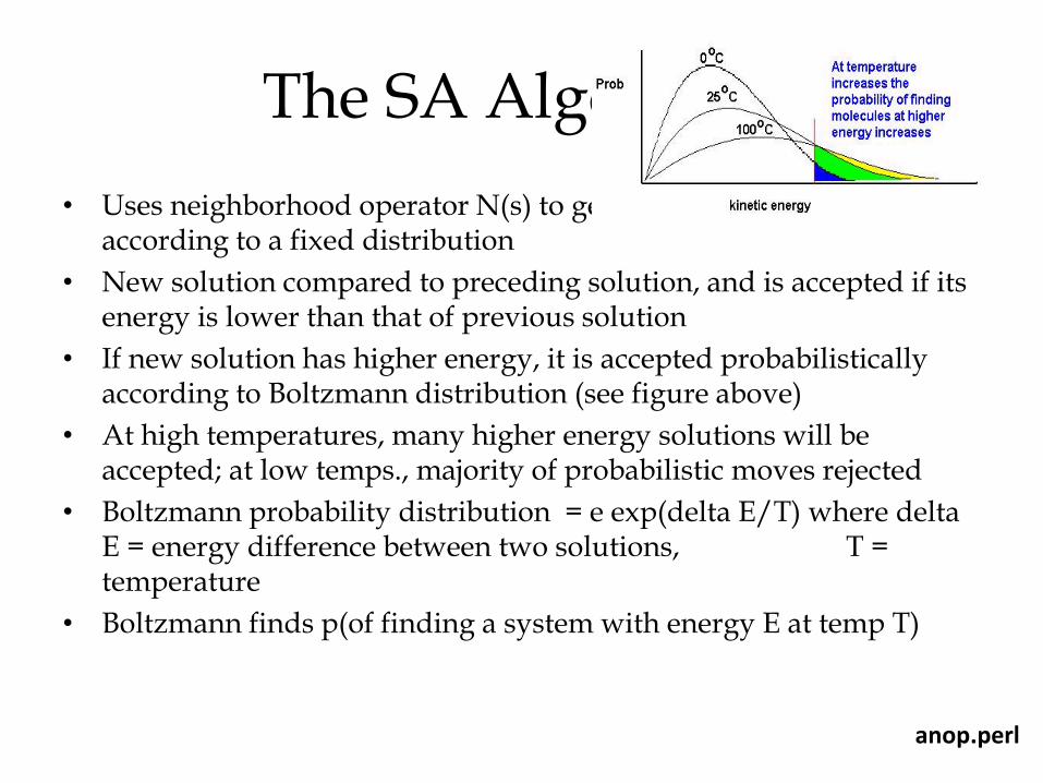
The SA Algorithm
• Uses neighborhood operator N(s) to generate a set of solutions according to a fixed distribution
• New solution compared to preceding solution, and is accepted if its energy is lower than that of previous solution
• If new solution has higher energy, it is accepted probabilistically according to Boltzmann distribution (see figure above)
• At high temperatures, many higher energy solutions will be accepted; at low temps., majority of probabilistic moves rejected
• Boltzmann probability distribution = e exp(delta E/T) where delta E = energy difference between two solutions, T = temperature
• Boltzmann finds p(of finding a system with energy E at temp T)
anop.perl
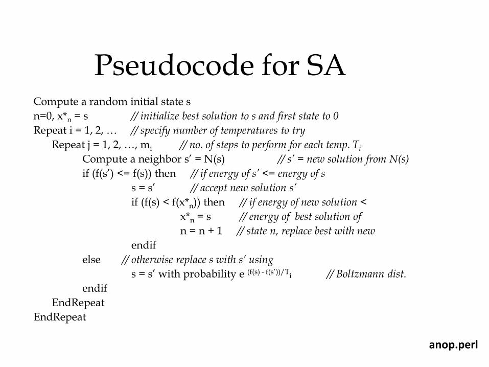
Pseudocode for SA Compute a random initial state s
n=0, x*n = s // initialize best solution to s and first state to 0
Repeat i = 1, 2, … // specify number of temperatures to try
Repeat j = 1, 2, …, mi // no. of steps to perform for each temp. Ti
Compute a neighbor s’ = N(s) // s’ = new solution from N(s)
if (f(s’) <= f(s)) then // if energy of s’ <= energy of s
s = s’ // accept new solution s’
if (f(s) < f(x*n)) then // if energy of new solution <
x*n = s // energy of best solution of
n = n + 1 // state n, replace best with new
endif
else // otherwise replace s with s’ using
s = s’ with probability e (f(s) - f(s’))/Ti // Boltzmann dist.
endif
EndRepeat
EndRepeat
anop.perl
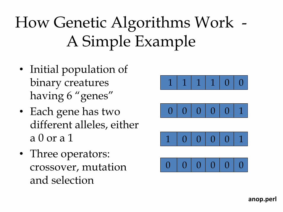
How Genetic Algorithms Work - A Simple Example
• Initial population of binary creatures having 6 “genes”
• Each gene has two different alleles, either a 0 or a 1
• Three operators: crossover, mutation and selection
1 1 1 1 0 0
0 0 0 0 0 1
1 0 0 0 0 1
0 0 0 0 0 0
anop.perl

Selection
• Selection based on a fitness function f(x)
• This operator chooses those individuals with the lowest values
• Those with higher values chosen with a very low probability
1 1 1 1 0 0
0 0 0 0 0 1
1 0 0 0 0 1
0 0 0 0 0 0
20
13
48
52
anop.perl
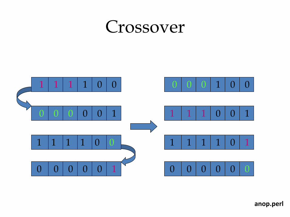
Crossover
0 0 0 1 0 0
1 1 1 0 0 1
1 1 1 1 0 1
0 0 0 0 0 0
1 1 1 1 0 0
0 0 0 0 0 1
1 1 1 1 0 0
0 0 0 0 0 1
anop.perl
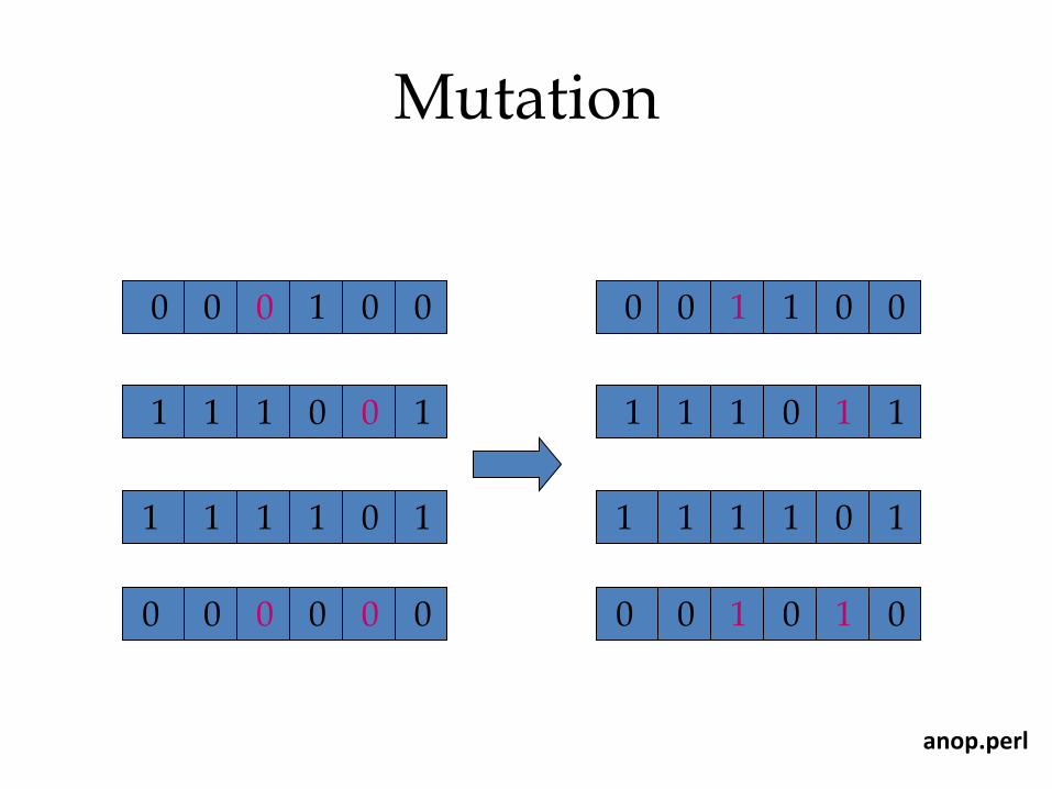
Mutation
0 0 1 1 0 0
1 1 1 0 1 1
1 1 1 1 0 1
0 0 1 0 1 0
0 0 0 1 0 0
1 1 1 0 0 1
1 1 1 1 0 1
0 0 0 0 0 0
anop.perl
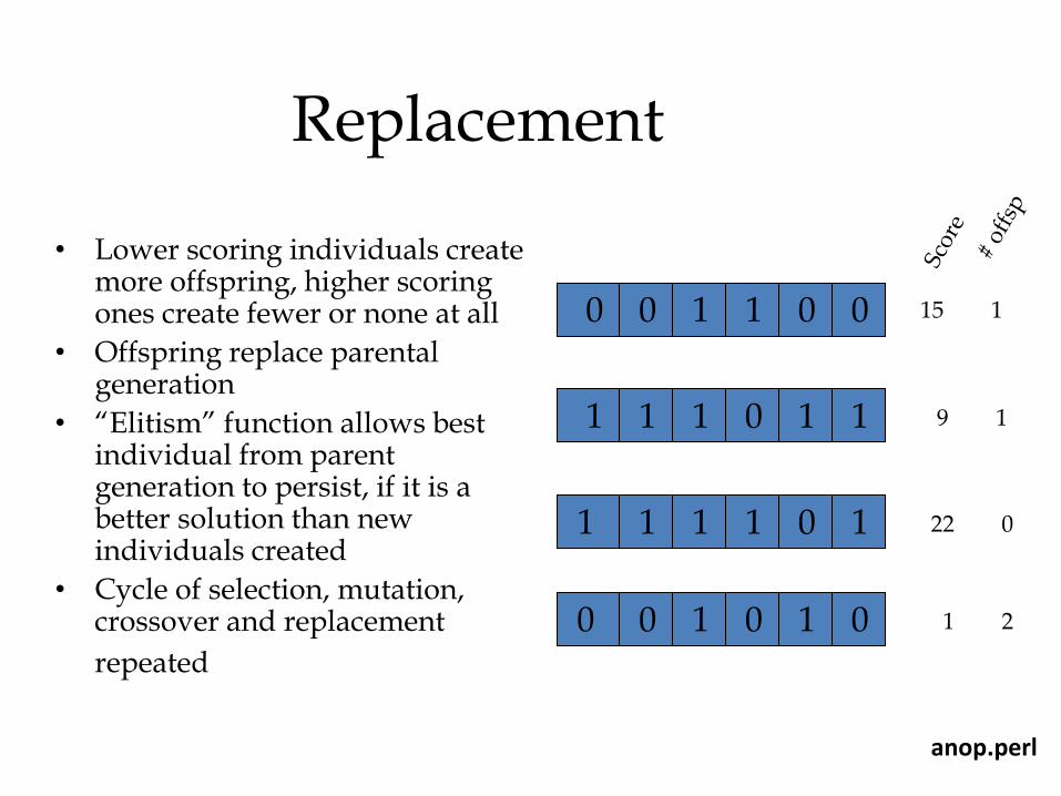
Replacement
• Lower scoring individuals create more offspring, higher scoring ones create fewer or none at all
• Offspring replace parental generation
• “Elitism” function allows best individual from parent generation to persist, if it is a better solution than new individuals created
• Cycle of selection, mutation, crossover and replacement
repeated
0 0 1 1 0 0
1 1 1 0 1 1
1 1 1 1 0 1
0 0 1 0 1 0
15 1
9 1
22 0
1 2
anop.perl
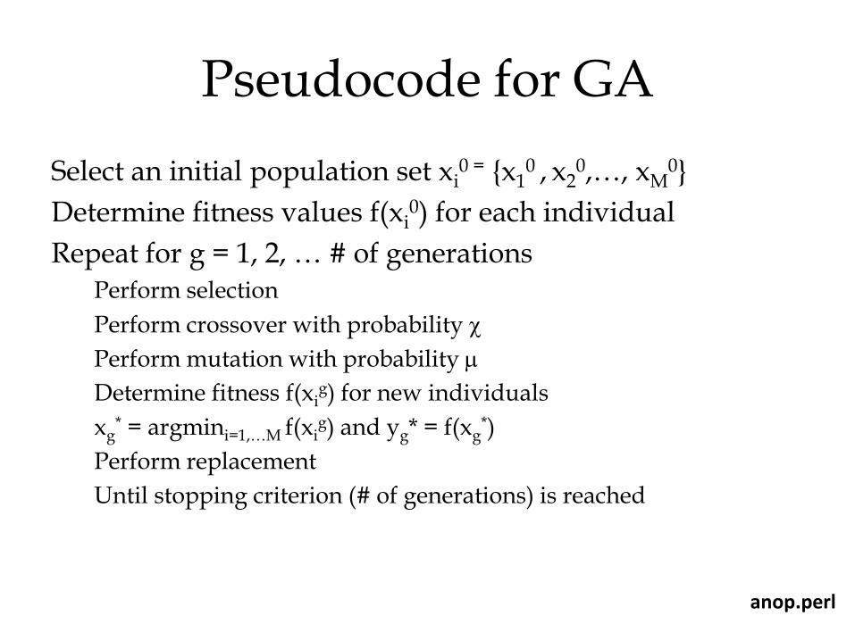
Pseudocode for GA
Select an initial population set xi0 = {x1
0 , x20,…, xM
0}
Determine fitness values f(xi0) for each individual
Repeat for g = 1, 2, … # of generations Perform selection
Perform crossover with probability
Perform mutation with probability
Determine fitness f(xig) for new individuals
xg* = argmini=1,…M f(xi
g) and yg* = f(xg*)
Perform replacement
Until stopping criterion (# of generations) is reached
anop.perl
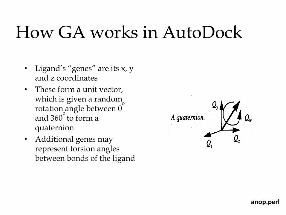
How GA works in AutoDock
• Ligand’s “genes” are its x, y and z coordinates
• These form a unit vector, which is given a random rotation angle between 0
o
and 360o
to form a quaternion
• Additional genes may represent torsion angles between bonds of the ligand
anop.perl
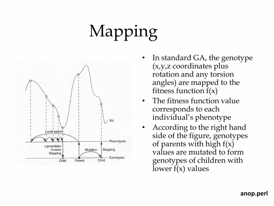
Mapping
• In standard GA, the genotype (x,y,z coordinates plus rotation and any torsion angles) are mapped to the fitness function f(x)
• The fitness function value corresponds to each individual’s phenotype
• According to the right hand side of the figure, genotypes of parents with high f(x) values are mutated to form genotypes of children with lower f(x) values
anop.perl
Selection, Crossover & Mutation • Selection chooses ligands with
the lowest fitness (energy) values
• Crossover exchanges x, y, z coordinates, or rotations or torsions between these ligands
• Example: Two ligands with xyz coordinates Abc and aBc Crossover results in new individuals with coordinates abc and ABc
• Mutation operator mutates coordinate or other angle values by adding a random real number according to a Cauchy distribution, which is similar to a Gaussian but has thicker tails
anop.perl
Replacement
• Individuals with better-than-average fitness receive proportionally more offspring
no= (fw – fi)/(fw - <f>),
fw != <f>
where
no= number of offspring
fi = fitness of individual (energy of ligand)
fw = fitness of worst individual in last g generations (typically 10)
<f> = mean fitness of population
anop.perl
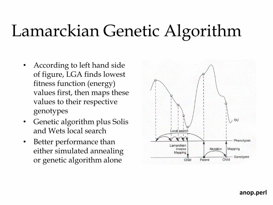
Lamarckian Genetic Algorithm
• According to left hand side of figure, LGA finds lowest fitness function (energy) values first, then maps these values to their respective genotypes
• Genetic algorithm plus Solis and Wets local search
• Better performance than either simulated annealing or genetic algorithm alone
anop.perl

Step
1. Coordinate file preparaEon
2. AutoGrid calculaEon
3. Docking using AutoDock
4. Analysis using AutoDock Tools (ADT)
anop.perl

• Get detail
autodock.scripps.edu/faqs.../autodock4.../AutoDock4.2_UserGuide.pdf
anop.perl