n -l d equations - byu physics and astronomy · differential equations are the language of physics,...
TRANSCRIPT

COMPUTATIONAL PHYSICS 330
NON-LINEAR DYNAMICS AND DIFFERENTIAL EQUATIONS
Ross L. Spencer and Michael Ware
Department of Physics and AstronomyBrigham Young University


COMPUTATIONAL PHYSICS 330
NON-LINEAR DYNAMICS AND DIFFERENTIAL EQUATIONS
Ross L. Spencer and Michael Ware
Department of Physics and AstronomyBrigham Young University
Last revised: May 21, 2018
© 2005–2018
Ross L. Spencer, Michael Ware, and Brigham Young University
Our objective in this course is to learn how to use numerical techniques toanalyze physics problems, with a focus on ordinary differential equations. Theinstructor and teaching assistants will highlight the important ideas and to coachyou through the laboratory exercises. This is not an independent study course.Students who try to work through this material on their own usually spend manyhours looking for trivial programming mistakes and consequently don’t have timeto learn the nonlinear dynamics which is at the heart of the course. Attendance atthe scheduled lab periods is critical.
We assume that you are already familiar with Mathematica, and we will oc-casionally use it to help with some of the symbolic manipulation. The first fewlabs focus on learning some of the necessary programming techniques. Later weuse both study nonlinear dynamics, including entrainment, limit cycles, perioddoubling, intermittency, chaos, ponderomotive forces, and hysteresis using Mat-lab. This course only provides a very brief introduction to nonlinear dynamics.To master this subject, you should pursue independent reading and take morecomplete courses in the subject.
Suggestions for improving this manual are welcome. Please direct them toMichael Ware ([email protected]).


Contents
Table of Contents v
1 Introduction to Matlab 1Basic Syntax . . . . . . . . . . . . . . . . . . . . . . . . . . . . . . . . . . . 1Writing Scripts . . . . . . . . . . . . . . . . . . . . . . . . . . . . . . . . . 1Loops, Logic, and Debugging . . . . . . . . . . . . . . . . . . . . . . . . . 2
2 Visualizations and Qualitative Analysis 5Line Plots . . . . . . . . . . . . . . . . . . . . . . . . . . . . . . . . . . . . 5How does a differential equation make a curve? . . . . . . . . . . . . . . 6
3 Phase Space and Matlab Functions 9Surface and Flow Plots . . . . . . . . . . . . . . . . . . . . . . . . . . . . . 9Phase Space . . . . . . . . . . . . . . . . . . . . . . . . . . . . . . . . . . . 9Functions in Matlab . . . . . . . . . . . . . . . . . . . . . . . . . . . . . . 11
4 Calculus and a Bouncing Ball 13Calculus on a Discrete Grid . . . . . . . . . . . . . . . . . . . . . . . . . . 13Roundoff . . . . . . . . . . . . . . . . . . . . . . . . . . . . . . . . . . . . . 14Numerical Solutions to Differential Equations . . . . . . . . . . . . . . . 14
5 Playing Baseball with ODEs 17Numerically Solving Differential Equations . . . . . . . . . . . . . . . . 17Baseball . . . . . . . . . . . . . . . . . . . . . . . . . . . . . . . . . . . . . 18
6 The Harmonic Oscillator and Resonance 21The Basic Oscillator . . . . . . . . . . . . . . . . . . . . . . . . . . . . . . 21The Damped Oscillator . . . . . . . . . . . . . . . . . . . . . . . . . . . . 21The Driven, Damped Oscillator and Resonance . . . . . . . . . . . . . . 23Resonance Curves . . . . . . . . . . . . . . . . . . . . . . . . . . . . . . . 23
7 The Pendulum 27The Simple Pendulum . . . . . . . . . . . . . . . . . . . . . . . . . . . . . 27Period and Frequency of the Pendulum . . . . . . . . . . . . . . . . . . . 27Differential Equations in Mathematica . . . . . . . . . . . . . . . . . . . 30
v

8 Two Gravitating Bodies 31Interpolation and Extrapolation . . . . . . . . . . . . . . . . . . . . . . . 32Linear Algebra . . . . . . . . . . . . . . . . . . . . . . . . . . . . . . . . . 33Center of Mass Coordinates . . . . . . . . . . . . . . . . . . . . . . . . . . 33
9 Fourier Transforms 37Fourier Transforms . . . . . . . . . . . . . . . . . . . . . . . . . . . . . . . 37FFTs and Fourier Transforms . . . . . . . . . . . . . . . . . . . . . . . . . 37The Uncertainty Principle . . . . . . . . . . . . . . . . . . . . . . . . . . . 38Windowing . . . . . . . . . . . . . . . . . . . . . . . . . . . . . . . . . . . 39
10 Pumping a Swing 41Pumping With Angular Momentum . . . . . . . . . . . . . . . . . . . . . 41Pumping With Parametric Oscillations . . . . . . . . . . . . . . . . . . . 43Interpreting the Spectrum of the Parametric Oscillator . . . . . . . . . . 44
11 The Pendulum with a High Frequency Driving Force 49Perturbation Theory . . . . . . . . . . . . . . . . . . . . . . . . . . . . . . 49Driven Pendulum . . . . . . . . . . . . . . . . . . . . . . . . . . . . . . . . 50
12 Chaos 53The van der Pol Oscillator . . . . . . . . . . . . . . . . . . . . . . . . . . . 53Limit Cycles and Attractors . . . . . . . . . . . . . . . . . . . . . . . . . . 53Entrainment . . . . . . . . . . . . . . . . . . . . . . . . . . . . . . . . . . . 54Dynamical Chaos . . . . . . . . . . . . . . . . . . . . . . . . . . . . . . . . 55Intermittency, 1/ f Noise, and the Butterfly Effect . . . . . . . . . . . . . 56Fractals . . . . . . . . . . . . . . . . . . . . . . . . . . . . . . . . . . . . . . 58
13 Coupled Nonlinear Oscillators 59Coupled Equations of Motion via Lagrangian Dynamics . . . . . . . . . 59Coupled Wall Clocks . . . . . . . . . . . . . . . . . . . . . . . . . . . . . . 61Solving Nonlinear Equations . . . . . . . . . . . . . . . . . . . . . . . . . 62
Index 65

Lab 1
Introduction to Matlab
Differential equations are the language of physics, but most of the interestingproblems involve differential equations that can’t be solved analytically. In thiscourse we’ll learn techniques to numerically solve differential equations with thegoal of studying interesting physics problems. Our first step is to learn the basicsof the Matlab programming language.
Basic Syntax
P1.1 Read and work through Introduction to Matlab, Chapter 1. Type and executeall of the material written in this kind of font. After you have workedthrough the chapter, use the Matlab command line to define the matrices
A=[1,2,3;4,5,6;7,8,9]
B=[1,4,5;9,6,3;2,3,1]
Also define the row and column vectors
v1=[1,1,2]
v2=[0.40824829 ; -0.81649658 ; 0.40824829]
(a) Use both * and .* to multiply A and B. Explain the difference.
(b) Perform the operation A./B and explain the result.
(c) Perform the operations A*v1, v1*A, and A*v2 and explain the results.
(d) Multiply only the center elements of A and B together
(e) Perform the operation exp(A+i*B) and explain what it means.
(f) Extract the center column of A, and then divide each element of thiscolumn by the corresponding element in v2.
Writing Scripts
P1.2 Read and work through Introduction to Matlab, Chapter 2. Type and executeall of the material written in this kind of font. Then complete thefollowing exercises:
(a) In your Freshman physics course, you learned that in the absence ofair resistance, a battleship’s projectile travels a horizontal distance
d = v2
gsin(2θ) ,
1
2 Computational Physics 330
where v is its initial speed and θ is the initial angle above the horizon-tal. Write a Matlab script that asks the user to enter a value for v in m/sand θ in degrees, and then calculates and prints the range formattedwith one decimal place, like this: “Range: 45.2 meters”. Rememberthat the standard trig functions are permanently set to use radians,but degree versions also exist. Use your program to find the properangle to hit a target exactly 10 km away if the initial velocity is 750 m/s.A battleship’s guns can’t elevate above 45 degrees.
(b) A planet’s velocity with respect to its star is v1 = 30000 x m/s when it ishit by an asteroid with velocity v2 = (−5000 x+8000 y+1000 z) m/s.The planet has mass m1 = 6×1024 kg and the asteroid has mass m2 =1×10¹⁹ kg. Write a script that defines the masses and velocities ofthe planet and asteroid using the variables m1, m2, v1, and v2. Thencalculate and display the final velocity of the planet after the collision:
v f =m1v1 +m2v2
m1 +m2
Your variables and your answer should be vectors. If it bothers youthat the planet’s velocity didn’t change, think about the precision youare using to display it.
Loops, Logic, and Debugging
P1.3 Read and work through Introduction to Matlab, Chapters 3-4. Type andexecute all of the material written in this kind of font, and run thecode in the listings.
(a) Write a script that uses a for loop to find the factors of 24 by testingevery number from 1 to 12 using the mod function. Once you are sureyour code correctly finds all of the factors of 12, use it to find all ofthe factors of 18648. To pass this exercise off, you must have at least 4comment lines in your code.
(b) Use a while loop to automate the process of finding the answer to thebattleship range problem in P1.2(a). Start the elevation at zero degreesand increase it in steps of 0.1 degrees until your range exceeds 5 km,and then break out of the while loop.
(c) Your roommate has borrowed $100,000 in student loans. The loancharges a 6% annual interest rate, and interest charges are appliedeach month. In other words, every month the loan charges a 0.5%interest fee on the remaining balance. This means that the amountby which you reduce your balance each month is not the amount youpay, but your payment minus the monthly interest. Your roommate

Lab 1 Introduction to Matlab 3
plans to pay your loan off by paying $1,000 per month. Write a pro-gram using loops and logic to calculate how long it will take to finishpaying off the loan. Don’t get fancy and derive an analytic formula forcompound interest payoff time. Just write a loop to track the balanceover time, and break out when the balance gets to zero.


Lab 2
Visualizations and Qualitative Analysis
Let’s start with some review of loops, logic, and matrices.
P2.1 Write a Matlab script that defines the following array
A=[14,42,91,79,95,65,3,84,93,67,75,74,39,65,17]
and then performs a “bubble sort” to order the array elements in A fromsmallest to largest. A bubble sort is a simple sorting algorithm that works
t The bubble sort is not an ef-ficient way to sort. Matlab’ssort command is much bet-ter, but we are learning howto program here.
by repeatedly looping through an array using a for loop, comparing eachpair of adjacent items and swapping them if they are in the wrong order.The for is nested inside a while that repeats until no swaps are needed inthe for loop. The algorithm gets its name from the way smaller elements“bubble” to the top of the list. Step through your code using the debuggingcommands while watching the values in A to make sure it is doing what youthink it should. To pass this exercise off, you must have at least 6 commentlines in your code.
Line Plots
Matlab has a wealth of visualization tools available to help you view your data.Let’s look at some of the 1-dimensional plotting tools.
P2.2 Read and work through Introduction to Matlab, Chapters 5. Type andexecute all of the material written in this kind of font and execute theexamples. Then complete the following exercises.
(a) Make a graph of f (x) = x sin(x) from x = 0 to x = 4π. Label the axesand give the plot a title. Then overlay on the same frame a plot ofcos(x) and add a legend to the plot that identifies each curve. UseMatlab help for the legend command to learn how to do this.
(b) Write a script with a for loop that calculates the first 20 terms of therecursion relation
a1 = 1 ; an+1 =(
n
(n −1/2)(n +1/2)
)an .
and stores each value in an array a. Use Matlab’s debugging com-mands to step through your code while you watch the values changein the workspace window. (HINT: a20 ≈ 1.3×10⁻¹⁷)
5

6 Computational Physics 330
When you are sure your program is working correctly, add some codeto plot the values of an versus n using semilogy. Then overlay plotsof e−n and 1/n! and label each line with a legend. Which function bestmatches the way the an terms fall off with n? You must have at leastfour comment lines in your code to pass it off.
(c) Define an array x that contains the values from x = 0 to x = 5 with astep size ∆x = 0.01. Make an empty array f the same size as x usingthe zeros command. Then use a for loop and logic commands toload f with the values:
f (x) ={
ex , 0 ≤ x < 1e ×cos(x −1) , 1 ≤ x ≤ 5
, (2.1)
Finally, plot f (x) vs. x and label your axes. You must have at least fourcomment lines in your script to pass it off.
HINT: For this problem do not use a command like
if x < 1
because x is an array, not a single number. You will need to addressindividual elements of the arrays when you do your logic tests andassignment statements.
How does a differential equation make a curve?
Our purpose in this course is to analyze problems with differential equations.Before becoming reliant on numerical ODE solvers, you need to develop anintuition for how differential equations behave. You will need this intuition topropose and refine mathematical models for physical processes and have a senseof whether the solutions that a computer spits out are reasonable. If you don’tdevelop good intuitive skills, the many differential equations you’ll encounter inyour physics courses will appear mysterious to you.
Let’s look at a simple differential equation and try to translate it into words:
d
d ty = y (2.2)
Since dd t y is the slope of the function y(t ) this differential equation says that the
bigger y gets the bigger its slope gets. Let’s consider the two possible cases forinitial conditions.
Case 1: y(0) > 0
The differential equation then says that the slope is positive, so y is increas-ing. But if y increases its slope increases, making y increase more, makingits slope increase more, etc. So the solution of this equation is a functionlike e t that gets huge as t increases.

Lab 2 Visualizations and Qualitative Analysis 7
Case 2: y(0) < 0
Now the differential equation says that the slope is negative, so y will haveto decrease, i.e., become more negative than it was at t = 0. But if y is morenegative then the slope is more negative, making y even more negative, etc.Now the solution is a strongly decreasing function like −e t .
Now consider another example. Suppose that you have discovered someprocess in which the rate of growth of the quantity y is not proportional to y itself,as in exponential growth, but is instead proportional to some power of y ,
d
d ty = y p (2.3)
This idea is referred to as “explosive growth.” Keeping in mind that with p = 1we get the exponential function, this equation says that if y starts out positive,y should increase even more than it did before, i.e., get bigger faster than theexponential function. That would have to be pretty impressive, and it is—y goesto infinity before t gets to infinity. Figure 2.1 shows a plot of the explosive growthfunction for the cases of P = 2 and P = 3.
Figure 2.1 The explosive growthfunction defined by Eq. 2.3 for twovalues of P .
You can play this qualitative analysis game with second-order differentialequations too. Let’s translate the simple harmonic oscillator equation
d 2
d t 2 y =−y (2.4)
into words. We need to remember that the second derivative means the curvatureof the function: a positive second derivative means that the function curveslike the smiley face of someone who is always positive, while negative curvaturemeans that it curves like a frowny face. And if the second derivative is large inmagnitude then the smile or frown is very narrow, like a piece of string suspendedbetween its two ends from fingers held close together. If the second derivative issmall in magnitude it is like taking the same piece of string and stretching yourarms apart to make a wide smile or frown.
So what does Eq. (2.4) say if y = 1 and y ′ = 0 to start? The first derivative iszero, so y(t ) comes out flat, and the second derivative is negative, so the functioncurves downward, making y smaller, which makes the frowniness smaller, butstill negative, so y keeps curving downward until it crosses y = 0. Then with ynegative the differential equation says that the curvature is positive, making ystart to smile and curve upward. It doesn’t curve much at first because y is prettysmall in magnitude, but eventually y will have a large enough negative valuethat y(t) turns into a full-fledged smile, stops going negative, and heads backup toward y = 0 again. When it gets there y becomes positive, the function getsfrowny and turns back around toward y = 0, etc. So the solution of this equationis an oscillation, cos(t ) or sin(t ).
P2.3 For each of the following cases, use qualitative analysis to sketch the solu-tion of the equation on paper.

8 Computational Physics 330
(a)d
d ty = y2 with y(0) =−1
(b)d 2
d t 2 y = y with y(0) = 1 andd
d ty(0) = 0
P2.4 Don’t start this problem until after making all of your sketches in P2.3.
(a) Verify, on paper, that the analytic solution to P2.3(a) is y(t ) =−1/(1+ t ) .Use Matlab to plot this function and compare it to your sketch.
(b) Verify that the analytic solution to P2.3(b) is y(t ) = (e−t +e t )/
2. UseMatlab to plot this function and compare it to your sketch.

Lab 3
Phase Space and Matlab Functions
Surface and Flow Plots
P3.1 Read and work through Introduction to Matlab, Chapter 6. Type and ex-ecute all of the material written in this kind of font and execute theexamples. Then do the following exercises:
Figure 3.1 The “mountain” func-tion.
(a) Write a script that makes a Matlab surface plot of the “mountain”function Fig. 3.1:
f (x, y) = e−|x−sin y |(1+ 1
5cos(x/2)
)(1+ 4
3+10y2
). (3.1)
Plot it from -5 to 5 in x and from -6 to 6 in y and add labels for thex and y axes. Make sure the labels correspond to the correct axes. Ifyour plot is solid black, don’t use such a fine grid in x and y .
(b) In a certain region of the atmosphere, the wind is blowing with velocitythat is constant in time, but varies spatially according to
d x
d t= vx = 0.2x2 +0.5y2 +20
d y
d t= vy =−0.1y3 +0.5x2 −10
(3.2)
Write a script that makes a quiver plot of the wind velocity over theregion -10 to 10 for x and y . Now add some stream lines beginning onthe left edge of your plot using the streamline command as shown inFig. 3.2.
Figure 3.2 Streamlines and windvelocity for the a wind velocityfield.
The plot you created in P3.2(b) is referred to as a flow plot. The arrows thatyou produced with the quiver command show the magnitude and the directionof the velocity at each point, and the streamlines show the path that a particlewould follow in this velocity field. You can also use this type of plot to understandthe behavior of differential equations.
Phase Space
You can often visualize the solution of a second-order differential equation with-out actually solving it using phase space1 techniques. In classical mechanics you
1R. Baierlein, Newtonian Dynamics (McGraw Hill, New York, 1983), p. 51-54, 140-144, and G.Fowles and G. Cassiday, Analytical Mechanics (Saunders, Fort Worth, 1999), p. 93-98.
9

10 Computational Physics 330
will learn to call the two-dimensional plane defined by the variables q and p = ∂L∂q
phase space (L is the Lagrangian). But for simplicity, in this lab we will use theposition x and velocity v as the phase space variables.
A second order differential equation can always be separated into a set offirst-order equations by defining an intermediate variable. For instance, a one-dimensional projectile with the constant acceleration is described by the differen-tial equation
d 2x
d t 2 =−g (3.3)
By defining an intermediate variable v , this second-order differential equationcan be written as a system of first-order differential equations like this:
d x
d t= v and
d v
d t=−g (3.4)
Notice that the position and velocity coordinates in Eq. (3.4) have the same formas the flow velocities in Eq. (3.2), i.e. the first derivatives on the left equal expres-sions on the right with no derivatives. If you think of d x/d t and d v/d t in Eq. (3.4)as flow velocities in the x-v plane, the right-hand sides of these equations tellyou what the “flow” velocity is at each point in space. At any point in time t , thecoordinate [x(t ), v(t )] gives the phase-space point that represents the “state” ofthe system. Given an initial starting point, you can then trace out a curve called aphase space trajectory analogous to the streamlines we plotted in the flow plot.
Part of the power of phase space flow plots is that you don’t have to solve thedifferential equation to make the flow plot. You just evaluate the right-hand sidesof Eq. (3.4), for example, and draw arrows at each point in the (x, v) space thatindicate which way the solution at that point will move if we take a small step intime. To draw the phase space trajectories, we just connect up the arrows overshort time intervals (or let Matlab do it for with with streamline). In this wayyou can explore the behavior of the system for a wide range of initial conditionswithout ever actually solving the ODE for any of these conditions.
P3.2 Sketch a phase space diagram for the one-dimensional projectile in Eq. (3.4)by hand on paper. Then draw some phase-space trajectories for a ball beingthrown up with various velocities. After you have done your work by hand,check it by using Matlab with the quiver and streamline tools.
P3.3 Make a phase space diagram for a simple harmonic oscillator given by:
d 2x
d t 2 =−x (3.5)
First sketch on trajectory by hand on a paper, then use Matlab to plotthe phase space diagram with many trajectories using the quiver andstreamline tools. Verbally describe the motion represented by each curve.

Lab 3 Phase Space and Matlab Functions 11
P3.4 Use Matlab to plot a phase space diagram for the angle of a rigid pendulum,given by
d 2θ
d t 2 =−sin(θ) (3.6)
Play with the range of the plot until you can clearly see motions that wig-gle back and forth, and others that just spin around like a propeller on aplane. Identify curves that are clockwise spinning, curves that are counter-clockwise spinning, and curves that wiggle back and forth.
P3.5 Use qualitative analysis to sketch the solution of the equation
d 2
d t 2 y =−y2 with y(0) = 1 andd
d ty(0) = 0
on paper like we did in the last lab. This ODE doesn’t have an analyticsolution. Make a phase-space quiver plot and use streamline to overlaya phase-space trajectory corresponding to the correct initial conditions andcompare this trajectory with your sketched solution and make sure they areconsistent.
Functions in Matlab
To this point, we’ve mostly relied on Matlab’s built-in functions tied together withsome code to perform our work. As our numerical techniques advance, we’ll needto be able to write our own functions. Pay close attention to this material, becauseit will be important throughout the remainder of the course.
P3.6 Read and work through Introduction to Matlab, Chapter 7. Type and executeall of the material written in this kind of font. Then do the followingexercises:
(a) Write an m-file function called EulerSum.m that computes the quan-tity
Se (N ) =(
N∑n=1
1
n
)− ln(N )
You can either use a loop or the sum command to compute the sum.Write a separate script that loads a variable Se with Se (N ) from N = 1to N = 1,000. Show that as N becomes large Se approaches a limit.This limit is called Euler’s constant, often represented by the Greekletter γ. To 15 digits, Euler’s constant is
γ= 0.577215664901532
Add a second output to EulerSum.m that returns the error |Se (N )−γ|.Use semilogy to plot this error as a function of N .

12 Computational Physics 330
(b) A square wave can be approximated by a sum of sine waves accordingto
f (x) =N∑
n=1,3,5,...an(x) (3.7)
where
an = 4
nπsin
(nπx
L
)(3.8)
Make an anonymous function that evaluates an(x) and then write aloop that evaluates f (x) for a given value of N . Use L = 1 and plotf (x) from -5 to 5. Notice that your function will need to accept twoarguments: n and x. Use your code to explore how big N needs to beto get a good approximation to a square wave. If you get a nice cleanpicture of a square wave, make your x grid finer and finer until yousee the Gibbs phenomenon spikes at the points of discontinuity thatyou learned about in Physics 318.

Lab 4
Calculus and a Bouncing Ball
For the past couple of labs we’ve focused on ways to visualize the solutions todifferential equations using phase-space plots and qualitative analysis. In this labwe’ll begin to learn how to solve differential equations numerically. To do this, werepresent functions of space and time using discrete grids rather than continuousvariables. Then we approximate derivatives as finite differences on this discretegrid rather than the infinitesimally small differences in analytic calculus. Webegin by exploring how to do calculus on grids. Then we’ll use these ideas todevelop a crude technique for numerically solving the differential equations for abouncing ball.
Calculus on a Discrete Grid
P4.1 Read and work through Introduction to Matlab, Chapter 8. Type and executeall of the material written in this kind of font. Then complete thefollowing exercises.
(a) Use the simple mid-point rule to numerically do the integral∫ 2
0x2e−x cos xd x . (4.1)
Experiment with different values of N until you are confident that youhave the answer correct to 6 decimal places. Then verify that you didit right by doing the same integral using Matlab’s integral commandwith an anonymous function.
(b) Consider the function f (x) = ex . The derivative of this function is ob-viously f ′(x) = ex , but imagine you didn’t know that, and numericallyevaluate f ′(x) at x = 1 using both the forward and centered differenceapproximation to the first derivative with a step size h = 0.5. Thencompare the approximations with the analytic answer (i.e. f ′(1) = e).
When you are sure you have the numerical derivatives coded correctly,switch h to be an array with values[
1
2,
1
4,
1
8, · · · ,
1
265
]Then write a for loop that calculates the error of the two derivative for-mulas as err=abs(fp/exp(1)-1) (where fp is the numerical deriva-tive) for each value of h, and stores the error in another array that
13

14 Computational Physics 330
is the same size as h. Finally, make overlaid loglog plots of the twoerrors vs. h. Show that the centered difference formula works better,but that both formulas are bad for very small values of h.
Explain why very small values of h make the approximate derivativebe wrong, giving zero instead of a good approximation to f ′. Thesection below on roundoff will be helpful.
Roundoff
The effect illustrated in exercise 4.1(b) is called roundoff and it rears its ugly headevery time you subtract two numbers on a computer. To understand round-off, consider the following two 15-digit numbers: a = 1.2345678912345 andb = 1.2345678918977. These are impressively accurate numbers, but their differ-ence is not so impressive: b−a = .0000000006632. Where did all of the significantdigits go; we started with 15 and now we only have 4? The problem is that thenumbers were so close together that subtraction made most of the significantfigures go away. When you work with numerical data on a computer you onlyhave a finite number of significant digits (15 in Matlab), so you have to be carefulwhen you subtract. And because subtraction is the key idea in differentiating, wehave to be careful about how we choose our step size h. As you can see in thisexercise, making it very small makes things worse, not better.
Numerical Solutions to Differential Equations
Now that we understand the basics of taking derivatives on a grid, let’s look at howto numerically solve differential equations. Consider the motion of a projectilenear the surface of the earth with no air resistance. The differential equationsthat describe the projectile are
d x
d t= vx
d y
d t= vy
d vx
d t= 0
d vy
d t=−g
(4.2)
along with some initial conditions, x(0), y(0), vx (0), and vy (0). This set of equa-tions is easily solved analytically, but imagine that we didn’t have an analyticsolution. How could we numerically model the motion of the projectile?
The basic idea behind a numerical solution is to think of your independentvariable (time in this case) as being a discrete grid rather than a continuousquantity. It is easiest represent time with an evenly spaced grid [t0, t1, t2, ...] witht0 = 0, t1 = τ, t2 = 2τ, etc. Then we label the dependent variables (space in thiscase) using the same indexing as the time grid, like this: x0 ≡ x(0), x1 ≡ x(τ),x2 ≡ x(2τ), etc. With this notation, we can write the equations in (4.2) using the

Lab 4 Calculus and a Bouncing Ball 15
(inaccurate) forward difference approximation of the derivative that you learnedabout in the reading:
xn+1 −xn
τ= vx,n
yn+1 − yn
τ= vy,n
vx,n+1 − vx,n
τ= 0
vy,n+1 − vy,n
τ=−g
(4.3)
Notice that the left sides of these equations are centered on the time tn+1/2, butthe right sides are centered at time tn . This makes this approach inaccurate, butif we make τ small enough it can work well enough to see the principles involved.
By solving the equations in (4.3) we can obtain a simple algorithm for steppingour solution forward in time:
xn+1 = xn + vx,nτ yn+1 = yn + vy,nτ
vx,n+1 = vx,n vy,n+1 = vy,n − gτ(4.4)
This method of approximating solutions is called Euler’s method. In general, it’st The name Euler does not
rhyme with “cooler”; itrhymes with “boiler”. Youwill impress your fellow stu-dents and your professorsif you give this importantname from the history ofmathematics its properpronunciation.
not very good, especially over many time steps. However, it provides a foundationfor learning other better methods.
P4.2 Make a program in Matlab to model the motion of a ball bouncing on thefloor using Euler’s method. In your script, define the initial position of theball with x=0 and y=1, and the initial velocity with vx=1 and vy=0. Thenwrite a while loop to step the position and velocity forward in time usingEq. (4.4). Have your while loop exit when x > 10. Use new variable namesfor the quantities at time level n +1, like this:
xnew = x + vx*tau;
vynew= vy - g*tau;
etc.
Then when you have advanced all four quantities, update the current valuesto get ready for the next step, like this:
xnew=x;
ynew=y;
etc.
(a) To simulate bouncing, put an if statement in your loop that checks ify is less than zero. When it is, make vy positive like this
vy=abs(vy)
Make a movie by plotting the position of the ball as a dot each timethe loop iterates, like this:
plot(x,y,'.')
axis([0 10 0 1.5])
pause(0.001)

16 Computational Physics 330
(b) Our bouncing condition in part (a) is lousy. Make it better by addingsome more logic that does the following:
(i) Test to see if y will go less than zero on this time step, but don’tactually change y yet.
(ii) If y won’t go less than zero this step, just do a regular Euler step.
(iii) If it will go negative this time step, determine a smaller time stepτ1 such that an Euler step will take the ball to y = 0. Then take anEuler step with τ1. After taking this small step, make the y-velocitypositive as before
vy=abs(vy)
and then take an Euler step of τ2 = τ−τ1 to finish off the time interval.
Play with different values of τ and notice that even with this improvedbouncing condition, Euler’s method is always unstable (i.e. the ampli-tude of the bounce continues to grow). This is a limitation of Euler’smethod, and we’ll develop better methods to overcome this shortcom-ing next time.
(c) Make your model look more realistic by adding some energy lossduring the bounce process by changing your bounce code to look likethis
vy=0.95*abs(vy)
This damping will mask the growth of Euler’s method for a suitablysmall τ.

Lab 5
Playing Baseball with ODEs
In the previous lab, we learned a crude method for numerically solving dif-ferential equations called Euler’s method. In this lab we learn how to take thenext step in refining that rudimentary technique into a more accurate ODE solver.After we have a good idea how ODE solvers are built and refined, we will introduceyou to some powerful differential equation solvers built into Matlab.
Numerically Solving Differential Equations
P5.1 Read and work through Introduction to Matlab, Sections 9.1-9.2. Type andexecute all of the material written in this kind of font. Then work thefollowing problems.
(a) Let’s start simple by modeling an object dropped from rest 10 m abovethe ground. Neglect air resistance, so that the gravitational force issimply F = mg . On a piece of paper, write down Newton’s secondlaw for this system and then convert it to a first-order set of coupledequations. Write the derivatives as finite differences on a grid in timelike we did in the last lab, and solve the resulting algebra equationsto derive the equations for Euler’s method. (Don’t peek at the answer,derive Euler’s method again from scratch.)
(b) Implement your equations from part (a) in a Matlab script to solve thedifferential equation. Keep track of all the values, and plot y(t ) untilyour object hits the ground. Overlay a plot of the analytic solution andcompare these plots for various values of τ.
(c) Modify your code from part (b) to use second-order Runge-Kutta.Evaluate how your accuracy changes as you vary τ, and overlay plotsof the Euler’s method solution, the Runge-Kutta solution, and theanalytic solution. Compare the answer for various values of τ.
P5.2 Read and work through Introduction to Matlab, Sections 9.3.
Important: As you work through this material in Introduction to Matlab,you will learn how to use an M-file named rhs.m to solve differential equa-tions. As you do this problem and in later labs, please don’t keep usingthe name rhs.m over and over. Invent a unique name, like rhs5_2.m, andchange the call to ode45 to correspond: ode45(@rhs5_2,...). This willmake it possible for you to come back later and see how you did each of theproblems.
17

18 Computational Physics 330
(a) Use Matlab’s numerical differential equation solver ode45 to solve themotion of the particle dropped from rest at a height of 10 m (no airfriction) by writing a rhs function and using Matlab’s ode45.
(b) Make another version of your code from part (a) that uses an anony-mous function instead of an external m-file rhs function. In subse-quent problems and labs, you are free to use either syntax, but whenthe functions get complicated its usually easier to use the external rhsfunction.
P5.3 Use Matlab’s ode45 to numerically solve the following equation.
d y
d t= y sin t ; y(0) = 1 (5.1)
Plot the numerical solutions from t = 0 to t = 100 and overlay a plot of theanalytic solution
y(t ) = e1−cos(t )
Fiddle RelTol and get a feel for how the accuracy changes with this param-eter. Note: this differential equation is only first order, so you won’t haveu(1) and u(2) this time. Think carefully about how to change your codefrom P5.2 to do this first-order problem.
Baseball
In Physics 121 you did the problem of a hard-hit baseball, but because you didit without air friction you were playing baseball on the moon. Let’s play ball in areal atmosphere now. The air-friction drag1 on a baseball is approximately givenby the following formula
Fdrag =−1
2Cdρairπa2|v|v (5.2)
where Cd is the drag coefficient, ρair is the density of air, a is the radius of the ball,and v is the vector velocity of the ball. The absolute value in Eq. (5.2) pretty muchguarantees that we won’t find a formula for the solution of this problem, but that’sfine since we know how to numerically solve differential equations now.
Figure 5.1 The trajectory for ahome run hit, including the effectof air friction. Note that the path isnot a parabola.
There are two forces acting on a baseball: air drag and gravity. Using Newton’ssecond law mr =∑
F, we see that equation of motion for the ball is
mr = Fdrag −mg y (5.3)
where r is the vector position of the ball, m is the mass of the baseball, g is theacceleration of gravity, and we have chosen the y direction to be up. Since this is
1For more information about the subject of air drag see R. Baierlein, Newtonian Dynamics(McGraw Hill, New York, 1983), p. 1-7, and G. Fowles and G. Cassiday, Analytical Mechanics(Saunders, Fort Worth, 1999), p. 55-65.

Lab 5 Playing Baseball with ODEs 19
a vector equation, it represents a system of equations—one for each dimension.To simplify our life, let’s consider the motion to be just in the x-y plane with x asthe horizontal direction. Using the definition of velocity, we can convert Eq. (5.3)into the following set of four coupled first-order equations
d x
d t= vx
d vx
d t=−
Cdρairπa2vx
√v2
x + v2y
2m
d y
d t= vy
d vy
d t=−
Cdρairπa2vy
√v2
x + v2y
2m− g
(5.4)
P5.4 (a) Use Matlab’s ODE solver to solve the set of equations (5.4) for a base-ball with the following parameters:
Cd = 0.35 ρair = 1.2 kg/m3
a = 0.037 m m = 0.145 kg
g = 9.8 m/s2
Put the point of contact between bat and ball at the origin (x(0) = 0,y(0) = 0). Write your initial conditions in terms of the initial angle θand velocity v0 of the baseball (i.e. v0x = v0 cosθ, v0y = v0 sinθ) so wecan play with the angle and initial speed.
Plot y(t ) and x(t ) for the initial conditions of θ = 45◦ and v0 = 60 m/s.Then plot the trajectory y(t ) vs. x(t ).
(b) Once you have your plot for the trajectory in air, overlay the trajectorythat the ball would have experienced without air drag on the sameplot. Estimate the difference in range caused by air friction.
(c) Power hitters say they would rather play in Coors Field in Denver thanin sea-level stadiums because it is so much easier to hit home runs.Do they know what they are talking about? To find out, repeat part (a),but instead of overlaying the no air friction plot, overlay the trajectoryof a ball hit in Denver and see if the ball goes significantly farther. Thedensity of air in Denver is about 15% lower than it is at sea level.


Lab 6
The Harmonic Oscillator and Resonance
The harmonic oscillator is probably the most studied system in dynamics. Inthis lab we use the numerical tools that we have developed to explore some ofthe behavior of this system.1 Before we dive into the computational details, let’sremind ourselves of the basic physics of a harmonic oscillator.
The Basic Oscillator
The basic oscillator equation is given by
d 2
d t 2 x(t ) =−ω20 x(t ). (6.1)
The solutions to this equation are just sines and cosines that wiggle forever intime with angular frequency ω0:
x(t ) = A sin(ω0t )+B cos(ω0t ) (6.2)
or equivalently,x(t ) = A sin(ω0t +φ) (6.3)
P6.1 (a) Sketch a phase space diagram for the harmonic oscillator by handon paper. Draw at least two phase-space curves for initial conditionsx(0) = 1, v(0) = 0 and another for x(0) = 0 and v(0) = 1.
(b) Use Matlab to make a phase-space plot of x(t) and v(t) for a simpleharmonic oscillator with ω0 = 2.
(c) Solve Eq. (6.1) numerically using Matlab’s ODE solver with initial val-ues x0 = 1 and v0 = 0, v0 = 1.4, and v0 =−1 and run them from t = 0to t = 1. Overlay the three trajectory plots on your flow plot. Identifyeach of the three initial conditions on your plot, and explain what theharmonic oscillator does along each trajectory.
Of course, no real oscillator wiggles forever. To model a real system we need toadd damping.
1You can read more about the simple harmonic oscillator in the following references: R. Baierlein,Newtonian Dynamics (McGraw Hill, New York, 1983), Chap. 2, and G. Fowles and G. Cassiday,Analytical Mechanics (Saunders, Fort Worth, 1999), Chap. 3.
21
22 Computational Physics 330
The Damped Oscillator
If we add some linear damping to the system, the harmonic oscillator equationbecomes
d 2
d t 2 x(t ) =−ω20 x(t )−2γ
d
d tx(t ), (6.4)
where the damping factor γ describes the amount of damping—a large γ meansthat there is a lot of damping. If you ask Mathematica to solve Eq. (6.4), it will tellyou that the solution is
x(t ) = Ae−t
(γ+pγ2−ω2
0
)+Be
−t(γ−pγ2−ω2
0
)(6.5)
Equation (6.5) looks impressive, but if it’s supposed to be an oscillator that damps,where are the sines and cosines? The problem is that we haven’t specified howbig ω0 and γ are yet. Let’s think physically for a minute.
Suppose that you put a pendulum in motor oil at 50 degrees below zero. Thisis an oscillator with a big γ. If you pull the pendulum back and release it, youare not going to see any swinging; the pendulum will just slowly ooze back tothe vertical position and stay there. We refer to this system as being overdamped.Look at Eq. (6.5) and convince your lab partner that this solution is made up ofdecaying exponentials when γ is big (specifically γ>ω0).
Now imagine what would happen if we decrease the damping, say by warmingthe oil up, or using WD-40 instead, or maybe even just air. In this case, thependulum will swing back and forth, but the amplitude will decrease over time.But by what miracle did the exponential functions in the original solution becomesines and cosines? Recall Euler’s formula
e iθ = cos(θ)+ i sin(θ)
which relates exponentials to wiggles through an imaginary argument. Note thatwhen γ<ω0, the square-root in Eq. (6.5) has a negative argument, and the squareroot is imaginary. In this situation, we can rewrite Eq. (6.5) as
x(t ) = e−tγ[
Ae−iωd t +Be iωd t]
(when γ<ω0) (6.6)
where the frequency at which the damped oscillator “wants” to wiggle is given by
ωd =ω0
√1−γ2/ω2
0 (6.7)
If the argument of this square root is positive (γ>ω0), then both of the fundamen-tal solutions in Eq. (6.5) are decaying exponentials and we only have damping(no wiggles). The transition between the two is when the argument of the squareroots is zero, i.e., when γ=ω0. This special case is called critical damping.
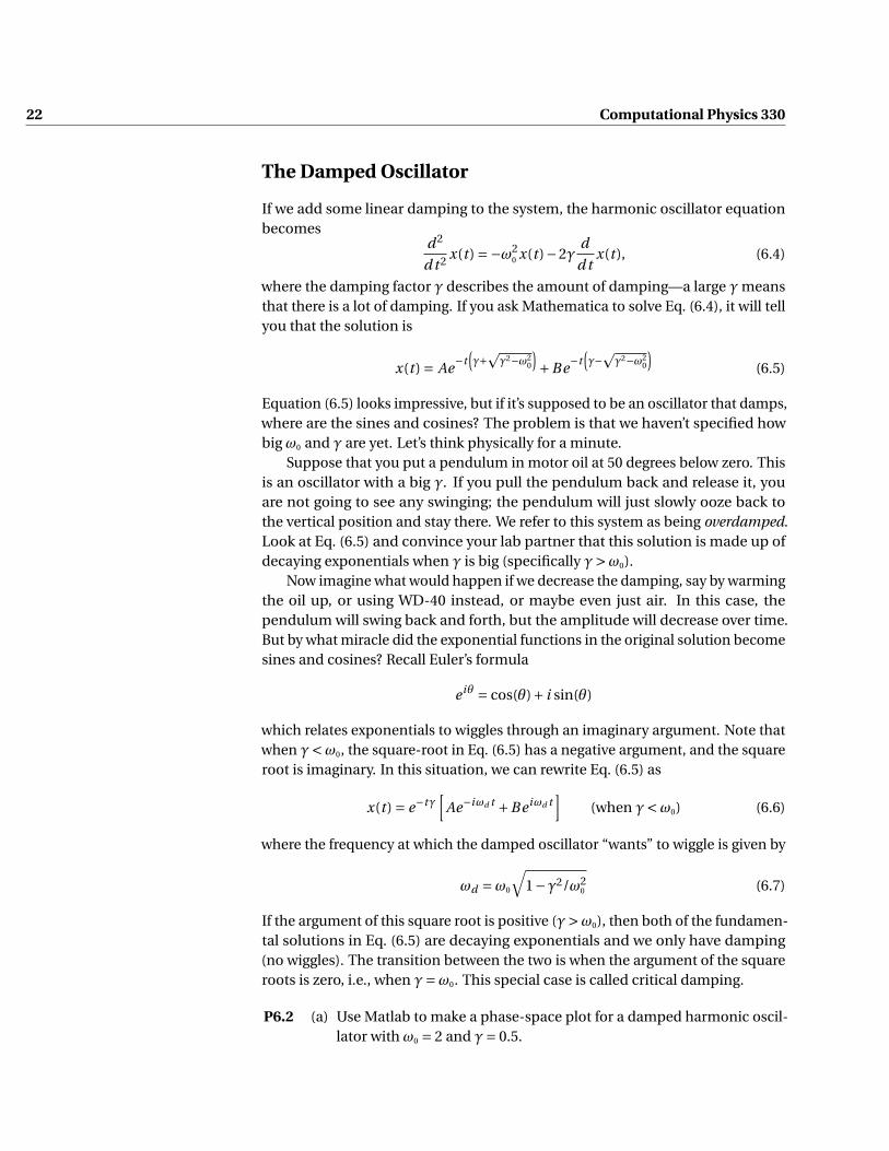
P6.2 (a) Use Matlab to make a phase-space plot for a damped harmonic oscil-lator with ω0 = 2 and γ= 0.5.

Lab 6 The Harmonic Oscillator and Resonance 23
(b) Solve Eq. (6.4) numerically using Matlab’s ODE solver with initial val-ues x0 = 1 and v0 = 0, v0 = 1.4, and v0 = −1, and run from t = 0 tot = 20. Overlay the three trajectory plots on your flow plot. Identifyeach of the three initial conditions on your plot, and explain what theharmonic oscillator does along each trajectory.
(c) Change the damping coefficient to γ= 4 and repeat (a) and (b). Ex-plain how the flow plot describes the overdamped system.
(d) An air-damped oscillator has damping more closely proportional tothe square of velocity rather than proportional to velocity. In equationform, we write this as
d x
d t= v ;
d v
d t=−ω2
0x −2γv |v | . (6.8)
Repeat (a) and (b), but change your model to use the quadratic air-damping in Eq. (6.8) with γ= 0.5 instead of linear damping. Explainhow this picture looks different from the ones in (a) and (b), and why.
The Driven, Damped Oscillator and Resonance
If we add a sinusoidal driving2 force at a frequency ω to the harmonic oscillator,the equation of motion becomes
d 2
d t 2 x(t ) =−ω20 x(t )−2γ
d
d tx(t )+ F0
mcos(ωt ) (6.9)
Now we have two frequencies in play—the driving frequency ω and the damped-oscillator frequency ωd given by Eq. (6.7). The typical behavior of the driven-damped harmonic oscillator starting from rest is as follows: an initial period ofstart-up with some beating between the two frequencies (ω and ωd ), then theoscillations at ωd damp out and the system transitions to a state of oscillation atthe driving frequency ω.
It is possible to solve Eq. (6.9) symbolically, but let’s study its behavior numer-ically for practice.
P6.3 Use Matlab to numerically solve Eq. (6.9) and plot x(t ) from t = 0 to t = 300with ω0 = 1, F0 = 1, m = 1, ω = 1.1, and γ = 0.01. Start from rest, withx(0) = 0 and x(0) = 0. Note the initial beating between frequencies andverify graphically that the final oscillation frequency of x(t ) is ω.
2For more information about the driven, damped harmonic oscillator, see: R. Baierlein, Newto-nian Dynamics (McGraw Hill, New York, 1983), p. 55-62, and G. Fowles and G. Cassiday, AnalyticalMechanics (Saunders, Fort Worth, 1999), p. 99-106.

24 Computational Physics 330
Resonance Curves
When you push someone in a swing, you find that if you drive the system at theright frequency, you can get large amplitude oscillations. This phenomenon is anexample of resonance, and the frequency at which the system has the maximumresponse is called the resonance frequency ωr . If you drive a system at a frequencyfar from ωr you only get small oscillations.
P6.4 (a) Make a new script by modifying your script from P6.3 so it makes aplot of x(t) starting from rest and running for a long time so all thebeating has stopped. Use F0 = 1, m = 1, γ = 0.1 ω0 = 1. Drive thesystem at ω= 1.1. Then write some code that measures the amplitudeof the steady-state oscillations using the colon command to selecta few cycles of oscillation at the end of the time period and the max
command to find the maximum value within these oscillations.
(b) Add a for loop to your code in (a) that varies the driving frequencyfromω= 0.5 toω= 1.5 in steps of∆ω= 0.2. For each driving frequency,use your code to measure the steady-state oscillation amplitude A(i.e. the amplitude of oscillation after all the beating has died out)and make a plot of the steady-state amplitude A versus the drivingfrequency ω. Note the region where this curve has a maximum valuesomewhere in the vicinity of ωd , but our resolution is too coarse tosee exactly where the maximum is.
(c) To better locate the maximum, modify your loop to look at the regionω= 0.98 toω= 1.02 with steps of∆ω= .001. Find the frequency wherethis curve has a maximum, and compare its location to ωd for thissystem. Are they the same?
In this problem you should note that the resonance frequency ωr (i.e. the peak ofthe resonance curve) is not the same as the same as the damped frequency ωd .When damping is small, ωr and ωd are close, but they are not the same.
The plot you made in P6.3 is called a resonance curve. A resonance curveplots the steady state oscillation amplitude (after the beating has died away)vs. the driving frequency. You did this by brute force, but for the simple driven-damped equation we can find an analytic solution for the resonance curve. Thesteady-state oscillation has the form
x(t ) = A cos(ωt −φ) (6.10)
where A is the steady state amplitude, ω is the driving frequency, and φ is thephase difference between the driving force and the oscillator’s response. Bysubstituting Eq. (6.10) into Eq. (6.9) and analyzing the result, we find that thesteady-state amplitude A is given by
A(ω) = F0/
m√(ω2
0 −ω2)2 +4γ2ω2(6.11)

Lab 6 The Harmonic Oscillator and Resonance 25
while the phase shift φ is given by
tanφ= 2γω
ω20 −ω2
. (6.12)
P6.5 (a) Write a matlab script that plots Eq. (6.11) for the parameters in P6.4and compare the plot with your numerical results. Also plot φ(ω) anddescribe to your lab partner what φ represents.
(b) Now make plots of A(ω) for several values of γ and verify that a smallerdamping coefficient γ leads to larger and sharper resonance.
(c) Show analytically that the peak of the resonance curve A(ω) is not atthe damped frequency ωd , but occurs at
ωr =√ω2
d −γ2 =√ω2
0 −2γ2 (6.13)
HINT: Remember that to find the peak of a curve, you take its deriva-tive and set it equal to zero.


Lab 7
The Pendulum
The harmonic oscillator is an incredibly useful system to understand becauseit is a reasonably good approximation to essentially every system that exhibitsoscillations, as long as the amplitude remains small. The classic example of aoscillating system is a simple pendulum. In this lab we’ll study how the pendulumresembles a harmonic oscillator and also how it differs.
The Simple Pendulum
The equation of motion of a simple pendulum is
θ =−ω20 sinθ , (7.1)
where θ is the angle (in radians) between the pendulum and the vertical directionand ω0 is the small-amplitude oscillation frequency. This is a nonlinear equation,so we often use the small angle approximation sinθ ≈ θ to simplify Eq. (7.1) into asimple harmonic oscillator. But it doesn’t take a very large amplitude before thesmall angle approximation falls apart. In this lab, we study the large amplitudebehavior of the pendulum, which can be quite different from the simple harmonicoscillator.
Figure 7.1 A phase space flow plotfor a pendulum.
P7.1 Show that Eq (7.1) is, in fact, nonlinear by showing that if you have two ofits solutions θ1(t ) and θ2(t ), then their sum θ1(t )+θ2(t ) is not a solution ofthe differential equation. When this happens, we say that the differentialequation is nonlinear. Use pencil and paper; Mathematica will just slowyou down.
P7.2 Use Eq. (7.1) with Matlab to make a phase space diagram with Matlab’squiver and streamline commands. Use this diagram to describe the pen-dulum behavior for small oscillations, large oscillations, and motion wherethe pendulum is rotating completely around rather than oscillating backand forth. Identify trajectories for both clockwise and counter-clockwiserotations.
Period and Frequency of the Pendulum
A pendulum is an extended object that is free to rotate with moment of inertia Iabout a pivot point. The distance from the pivot point to the center of mass of theobject is `, and the small-amplitude oscillation frequency is ω0 =
√mg`/I . If the
27

28 Computational Physics 330
pendulum is a simple massless stick of length ` with all of the mass at the end ofthe stick, the small-amplitude oscillation frequency simplifies to ω0 =
√g /`.
Figure 7.2 A simple pendulumcomprised of a massless stick oflength ` with a mass m at the end.
We can find the large-amplitude oscillation frequency of the pendulum byusing an energy method.1 The kinetic energy of the pendulum is I θ2/2 and thepotential energy is mg`(1−cosθ) (see Fig. 7.2). The total energy of a pendulumcan be found when the pendulum is at the maximum displacement, which wewill denote by θ0. At this point, the center of mass is at a height of `(1−cosθ0)above the equilibrium position and the kinetic energy is zero, so the total energyis mg`(1− cosθ0). As the pendulum oscillates, energy shuttles back and forthbetween kinetic and potential according to
1
2I θ2 +mg`(1−cosθ) = mg`(1−cosθ0) (7.2)
The first term on the left is the kinetic energy, the second term is the potentialenergy, and the right side is the total energy of the system.
P7.3 Using paper and pencil, separate the variables θ and t in Eq. (7.2) and showthat it can be written as
ω0d t = dθ√2cosθ−2cosθ0
(7.3)
Figure 7.3 The frequency of a pen-dulum depends on the amplitudeof oscillation. The variation of fre-quency with amplitude is smallestfor low-amplitude oscillations, soits easier to get good accuracy withlong pendulum and small angleoscillations as in a grandfatherclock.
To find the period of oscillation, we integrate both sides of Eq. (7.3) over aquarter period of the motion (from θ = 0 to θ = θ0 on the angle side and fromt = 0 to t = T /4 on the time side), like this
ω0
∫ T /4
0d t = 1p
2
∫ θ0
0
dθ√cosθ−cosθ0
(7.4)
The time integral on the left is simply ω0T /4, but the θ integral on the right isdifficult. After carrying out the time integral and performing some judiciousvariable substitutions and a little algebraic massaging, we can rewrite Eq. (7.4) as
T = 4
ω0
∫ π/2
0
dφ√1− sin2(θ0/2)sin2φ
(7.5)
The φ integral in Eq. (7.5) is not any easier than the θ integral in Eq. (7.4), but ithas come up in enough problems that it has been given a name: the completeelliptic integral of the first kind, called K (m):
K (m) ≡∫ π/2
0
dφ√1−m sin2φ
(7.6)
1 G. Fowles and G. Cassiday, Analytical Mechanics (Saunders, Fort Worth, 1999), p. 318-320

Lab 7 The Pendulum 29
Matlab and Mathematica know how to evaluate K (m) functions for 0 ≤ m ≤ 1 justlike they can evaluate sines, cosines, and Bessel functions. Thus, we can write theperiod T of the pendulum as
T = 4
ω0K
(sin2(θ0/2)
)(7.7)
Now we can use the relation ω = 2π/T to obtain an expression for the angularfrequency of the pendulum as a function of amplitude θ0.
ω(θ0) = πω0
2K(sin2(θ0/2)
) (7.8)
00
Figure 7.4 Oscillation frequencyas a function of the maximumamplitude θ0.
Note that the natural oscillation frequency ω(θ0) of the pendulum dependson amplitude θ0, as shown in Fig. 7.4. This gives the pendulum some interestingcharacteristics.
P7.4 Use Matlab to plot ω(θ0) from θ0 = 0 to θ0 = π with ω0 = 1 and explainphysically why it looks like it does. In particular, explain why the frequencygoes to zero at θ0 =π. You’ll need to use the online help to see the syntaxfor evaluating the elliptic integral function.
Now let’s solve the pendulum equation numerically using Matlab.
P7.5 Use Matlab’s numerical differential equation solver ode45 to solve the pen-dulum, again with ω0 = 1 and initial conditions θ(0) = θ0 and ω(0) = 0. Plotthe solution θ(t ) for the following values of θ0: 0.1, 0.5, 1.0, π/2, 0.9π, and0.98π. For each case overlay a plot of a cosine function of matching ampli-tude and with a frequency ω(θ0) from Eq. (7.8). Verify that Eq. (7.8) givesthe correct frequency, but that for large amplitudes the pendulum motionis not sinusoidal.
P7.6 Now let’s study what happens when we add driving and damping.
(a) First we’ll review what happens when we drive an undamped har-monic oscillator. Write a Matlab script that solves the driven oscillatorequation
y +ω20 y(t ) = F0 sin(ωt ) (7.9)
and plot the solution y(t) with ω0 = ω = 1. Start from rest and runfor a long enough time that you can see the amplitude heading off toinfinity, even with small values of F0.
(b) Now drive an undamped pendulum with an external torque, like this
θ+ω20 sinθ =αsinωτt . (7.10)
Drive the pendulum at resonance for small amplitudes, with ω0 = 1,ωτ = 1, and α= 0.1. Start at rest and run for a long enough time thatyou can see that the pendulum amplitude doesn’t simply go to infinitylike the harmonic oscillator. Explain why not.

30 Computational Physics 330
(c) Finally, add some linear damping, to the pendulum equation like this:
θ+ω20 sinθ =αsinωτt −γθ . (7.11)
Use γ = 0.1 and the same conditions as in (b) and watch how themotion changes. Explain the damped behavior and explore howit depends on α. Also vary the driving frequency ω in the range0.90ω0 → 1.05ω0 and explain why ω = ω0 doesn’t give the largestamplitude.
Differential Equations in Mathematica
While the focus of this course is on learning numerical techniques in Matlab,Mathematica also has some excellent differential equation solving abilities thatyou should be aware of. Let’s take a break from Matlab and learn some of thebasics in Mathematica.
P7.7 Read the section titled “Symbolic solutions to ordinary differential equa-tions” in the Mathematica tutorial Differential equations with Mathematica(available on the Physics 330 course web page).
P7.8 Use Mathematica to solve the following differential equations in generalform (no initial conditions).
(a) Bessel’s Equation
x2(
d 2
d x2 f (x)
)+x
(d
d xf (x)
)+ (x2 −n2) f (x) = 0
(b) Legendre’s Equation
(1−x2)
(d 2
d x2 f (x)
)−2x
(d
d xf (x)
)+n(n +1) f (x) = 0
P7.9 Read the section titled “Numerical solutions to ordinary differential equa-tions” in the Mathematica tutorial Differential equations with Mathematica.
(a) Ask Mathematica to solve the following differential equation symboli-cally and see what happens.
d 2
d x2 y(x) = 10sin(y (x)
)cos(x) (7.12)
Now write the equation as a first order set, and solve it numericallywith y(0) = 0 and v(0) ≡ y ′(0) = 0.1. Plot y(x) from x = 0 to x = 100.

Lab 8
Two Gravitating Bodies
Let’s continue our study of differential equations by considering two massesinteracting through Newton’s law of gravity.1 The Newton’s second-law equationsdescribing this situation are
m1r1 =− Gm1m2
|r1 − r2|3(r1 − r2) (8.1)
m2r2 =− Gm1m2
|r1 − r2|3(r2 − r1) (8.2)
wherer1 = x1x+ y1y+ z1z
r2 = x2x+ y2y+ z2z
There are twelve components of the motion described by these equations:
x1(t ), y1(t ), z1(t ) x1(t ), y1(t ), z1(t )
x2(t ), y2(t ), z2(t ) x2(t ), y2(t ), z2(t )(8.3)
so you’ll need to be careful when writing out the solution.
−4 −2 0
05
10−8
−6
−4
−2
0
y
Two Masses Orbiting and Drifting
x
z
Figure 8.1 Two masses interactingvia the inverse-square law.
P8.1 (a) Use Eqs. (8.1) and (8.2), plus x1 = vx1, etc., to obtain the 12 first orderdifferential equations for this system. Write them down on paper interms of the individual components of the motion listed in Eq. (8.3).
(b) Now use your information from (a) to code up a right-hand-side func-tion for this system. Have Matlab solve this system of equations usingG = 1, m1 = 1, m2 = 2 and initial conditions
x1(0) = 1, x2(0) =−1y1(0) = 0.5, y2(0) =−0.3z1(0) =−0.3, z2(0) = 0.6vx1(0) = 0.65, vx2(0) =−0.45vy1(0) = 0.2, vy2(0) = 0.3vz1(0) = 0.1, vz2(0) =−0.3.
Run the solution from t = 0 to t = 50, and then plot the two trajectoriesoverlaid on the same plot using plot3.
1R. Baierlein, Newtonian Dynamics (McGraw Hill, New York, 1983), Chap. 5, and G. Fowles andG. Cassiday, Analytical Mechanics (Saunders, Fort Worth, 1999), Chap. 6.
31

32 Computational Physics 330
A plot like Fig. 8.1 gives us some sense of how these two objects interact, butit doesn’t show what the dynamics of this system are like. For that, it would bebetter to make a movie of the interaction by plotting the positions as dots, andthen making a movie by showing successive plots at equal time intervals.
The problem with making movies directly from the data returned by Matlab’sODE solvers is that the data that Matlab’s ODE solver returns is not equally spacedin time. You can force the Matlab functions to return equally-spaced data bygiving it a list of specific times for which you want the solution evaluated, but thisis computationally expensive if you need a lot of closely spaced time intervals.A better approach is to get the uneven data back from the solver and then useinterpolation to resample it out over a much finer grid.
Interpolation and Extrapolation
P8.2 Read and work through Introduction to Matlab, Chapter 10. Type andexecute all of the material written in this kind of font. Then write aMatlab script that creates coarse and fine grids for sin x like this
x=0:2*pi;
y=sin(x);
xfine=-2*pi:0.1:2*pi;
yfine=sin(xfine);
Use linear interpolation to plot a line using the fine grid that passes throughy(1) and y(2). Then use the pchip method (cubic interpolation) andthe spline method to plot a curve on the fine grid that passes throughy(1), y(2), and y(3). Overlay all of the curves: the coarse plotted asstars, the fine and the interpolated curves as lines. Use these curves toexplain the benefits and hazards of using linear and cubic interpolationand extrapolation.
P8.3 Now let’s go back to your code from P8.1. After obtaining the solutionarrays interpolate them onto new arrays equally spaced in time (x1e, y1e,
z1e, x2e, y2e,... with N=5*length(t)). The point here is to make anevenly-spaced array of time points with 5 times as many time values asode45 returned, but covering the same amount of time. This can be done bydefining the evenly-spaced time interval dt=t(end)/N and then buildingthe evenly spaced time array like this:
te=0:dt:t(end)
Then use interp1 to build evenly-spaced position data like this:
x1e=interp1(t,x1,te,'spline')
Now animate the motion of the two masses by using the plot3 command.A nice way to do this animation is to use the arrays that are equally spacedin time, so that you can see the masses speed up as they approach each

Lab 8 Two Gravitating Bodies 33
other, and to plot the orbits in segments of 5, or so, data points. Using justone point makes the orbits appear as sequences of dots, and using morepoints makes the plots be “jerky.” A loop that will do this kind of animationis shown below:
for n=5:4:N
plot3(x1e(n-4:n),y1e(n-4:n),z1e(n-4:n),'b-');
hold on
plot3(x2e(n-4:n),y2e(n-4:n),z2e(n-4:n),'r-');
axis equal;
pause(.1)
end
hold off
As your script runs you should see your masses doing an intricate gravita-tional dance, and the final picture should look just like the one in Fig. 8.1(after the appropriate rotation of your figure).
Linear Algebra
P8.4 Read and execute the examples in Introduction to Matlab, Chapter 11. Thencomplete the following exercises.
(a) Use Matlab’s dot command to find the angle between the vectorsA = [1,2,3] and B = [−3,2,1].
HINT: You will need to calculate the magnitude of a vector to do thisproblem.
(b) Use Matlab’s cross command to find the angular momentum L =mr×v of a particle at r = [1,2,3] with velocity v = [6,3,1] and massm = 2.3.
Center of Mass Coordinates
In physics we always seek the simplest description of the motion, which is why inclassical mechanics we trade in r1 and r2 for the center of mass position and therelative position of m1 with respect to m2:
R = m1r1 +m2r2
m1 +m2; r = r1 − r2 (8.4)
P8.5 (a) Use plot3 to graph R and V = R for the initial conditions in P8.1and show that their motion is very simple. To do the calculationsin Eq. (8.4) it will be easier to transform the separate x, y , and z arraysinto vectors. For instance, the r1 vector would be a matrix with 3columns and as many rows as there were time steps. For example tomake the matrix representing r1(t ), you would use code like this:

34 Computational Physics 330
r1=[x1,y1,z1];
Also define versions of these vectors with the data equally spaced intime so we can animate some plots. Once you have the R matrices,you can access the various components using the colon syntax. Forexample R(:,1) gives the x-component of R etc.
(b) Make a 3d plot of the difference vector r and use the frame rotationtool on the figure frame to see that this vector seems to sweep out acurve that lies in one plane and looks like an ellipse. Then animateyour plot to show the orbit as a function of time.
(c) To see why the difference motion r(t) lies in a plane, compute theangular momentum in the center of mass frame
L = m1(r1 −R)× (v1 −V)+m2(r2 −R)× (v2 −V) (8.5)
and show numerically that this vector is constant in time. Since youhave the vectors that appear on the right-hand side of this expressionfor L you can evaluate the angular momentum as a matrix (rows aretime, columns are x, y, z components):
L=m1*cross(r1-R,v1-V)+m2*cross(r2-R,v2-V);
And then plot each component of the angular momentum vs. time.
(d) Show graphically that L is perpendicular to both r1−R and r2−R (andhence to r1 − r2). To evaluate these two dot products using Matlab’sdot command you will need to make a slight change to the syntaxwe used above with the cross command. The dot command whenused with matrices needs to know whether we want to do the dotproduct along the row direction or the column direction. In this labthe rows label time, and the columns label x, y, z components. Sincewe want to do the dot product with the x, y, z components, we tell thedot product command to use the second, or column, index like this:
dot1=dot(r1-R,L,2)
dot2=dot(r2-R,L,2)
Do not panic when your plots of these two dot products look surpris-ing; check the scale on the left side of the plot. Note that this meansthat the planar motion you observed in the plot of r is simply a conse-quence of conservation of angular momentum (think about this anddiscuss it with your lab partner until you are convinced that it is true).
−1 −0.5 0 0.5 1−1
−0.5
0
0.5
1
x
y
Non−inverse Square Law
Figure 8.2 Precession of the orbit,non-inverse-square.
P8.6 Play around with initial condition and plot r(t ) for a bunch of cases to seewhat orbital shapes you can observe. Then choose some initial conditionsthat make a nice ellipse. Once you have an ellipse, change the power in thedenominator of the force law from 3 to 3.1 to see what kinds of orbits powerlaws other than inverse square make. You should find that the orbit is stillsort of elliptical, but that the semi-major and semi-minor axes rotate; wecall this kind of motion “precession” and it looks like Fig. 8.2.

Lab 8 Two Gravitating Bodies 35
In general relativity the gravitational force law is not precisely inverse-square, so this kind of precession is expected to occur. Mercury’s orbithas a small precession of this kind (the famous “precession of the equinoxof Mercury”) which has been measured for centuries. When Einstein’sequations correctly predicted this precession it was a major triumph for histheory of general relativity.


Lab 9
Fourier Transforms
Fourier Transforms
Suppose that you went to a Junior High band concert with a digital recorder andmade a recording of Mary Had a Little Lamb. Your ear told you that there were awhole lot of different frequencies all piled on top of each other, but perhaps youwould like to know exactly what they were. You could display the signal on anoscilloscope, but all you would see is a bunch of wiggles. What you really want isthe spectrum: a plot of sound amplitude vs. frequency.
The mathematical method for finding the spectrum of a signal f (t) is theFourier transform
g (ω) = 1p2π
∫ ∞
−∞f (t )e iωt d t (9.1)
If you remember Euler’s relation e iωt = cos(ωt)+ i sin(ωt), you can see that thereal part of g (ω) is the overlap of your signal with cos(ωt) and the imaginarypart of g (ω) is the overlap with sin(ωt ).1 Often, we aren’t interested in the phaseinformation provided by the complex nature of g (ω), so we just look at the powerspectrum P (ω)
P (ω) = |g (ω)|2 (9.2)
P (ω) gives the signal intensity as a function of frequency without any phaseinformation. In this lab, we will learn how to make these types of plots.
FFTs and Fourier Transforms
Power Spectrum (linear scale)
Power Spectrum (log scale)
Figure 9.1 The power spectrum ofthe first four notes of Beethoven’s5th symphony.
P9.1 Read and work through Introduction to Matlab, Chapter 13. Type andexecute all of the material written in this kind of font.
P9.2 On the class web site is a file called “Beethoven.wav” that has the first fournotes of Beethoven’s 5th symphony. Save it to your computer and listen toit. Load the sound waveform into the matrix f using
f = audioread('beethoven.wav');
Then construct the corresponding t time series by noting that the recordingwas sampled at 44100 points/second. Plot the signal versus time and plotits power spectrum versus ν (not ω) over the range 0-1000 Hz with both alinear scale and with semilogy. (You should get in the habit of looking at
1People often work with complex signals, in which case this separation is less clear.
37

38 Computational Physics 330
spectra with a log scale to see structure that may not be evident on a linearscale.)
Now we need to make sense of the spectrum. The short notes at the begin-ning of the music are the note “G” (repeated three times) played in octavesby the violins/violas (394 Hz), cellos (197 Hz), and basses (99 Hz). The lastnote is an “E-flat,” again played in octaves by the various stringed instru-ments (312 Hz, 156 Hz, and 78 Hz). Identify each of these peaks on thespectrum, and explain what their relative amplitudes mean.
Figure 9.2 A string’s fundamen-tal mode of vibration has nodesat the ends and an antinode inthe middle. However, the stringcan also vibrate in harmonicmodes with nodes between theends. When a musician dragsher bow across a string, sheexcites mostly the fundamen-tal, but the harmonics are alsopresent. The frequencies of thesemodes are: ν0 = fundamental,2ν0 = second harmonic, 3ν0 =third harmonic, etc.
Note that there are also smaller peaks at 234 Hz, 468 Hz, 624 Hz, 788 Hz,and 936 Hz. Explain where these extra peaks come from, and how each ofthe smaller peaks are connected to the notes in the four-note theme (seeFig. 9.2).
To convince yourself that you know what you are doing, split the time seriesinto two pieces: one that contains the first three short notes, and a secondthat only contains the one last long note. Then repeat the analysis aboveand compare your two new spectra to the original one. Show the TA allthree spectra and explain the origin of all of the peaks.
The Uncertainty Principle
The uncertainty principle connects the duration of a signal in time with thespread of its spectrum. It was made famous in quantum mechanics by WernerHeisenberg, but it is really an idea from classical wave physics2 which we canunderstand by using the fft.
Suppose that we have a time signal which has a frequency ω0, but which onlylasts for a finite time ∆t . For example, consider the Gaussian function
f (t ) = cos(ω0t )e−(t−t0)2/W 2(9.3)
which has a “bump” centered at t0 with a width controlled by W . Because thesignal oscillates at ω0 we would expect to see a peak in the spectrum at ω=ω0.This frequency peak also has a well-defined width, and this width is related to thewidth of the signal in time through the uncertainty principle.
P9.3 Write a Matlab script to build f (t) from Eq. (9.3), with t0 chosen so thatthe bump is in the center of your time window. Plot f (t) and its powerspectrum for ω0 = 200 s−1 and W = 10, 1, and 0.1.
Choose appropriate values for your number of points N and your time stepτ so that
(i) fft will run fast
2The weirdness of quantum comes not from the fact that waves obey the uncertainty principle,but from the idea that things like electrons behave like waves.

Lab 9 Fourier Transforms 39
(ii) you can see frequencies up to ω= 400 s−1 without aliasing trouble
(iii) your spectral resolution will be at least dω= 0.2 s−1.W ∆t ∆ωplot ∆t∆ωplot
101
0.1
Table 9.1 Enter your data here
To see where the uncertainty principle is lurking in these plots, visuallymeasure and write down the full width at half maximum (FWHM) of thetime signal (∆t) and FWHM of the frequency peak (∆ωplot). Write thesemeasurements in Table 9.1 for each value of W . Then deduce a roughproduct relation ∆ω∆t ≈ const between the width of the time signal andthe width of the frequency peak from this data.3
You have probably experienced the uncertainty principle when listening tomusic. For a musical instrument to play a nice-sounding note the width of itsspectrum must be narrow relative to the location of the peak. So for a flute playinga high note at ω= 6000 s−1 to produce a spectrum with, say, a 1% width requires∆ω= (0.01)(6000 s−1) = 60 s−1. Then the uncertainty principle tells us that thisnote can be produced by only holding it for the relatively short time of
∆t ≈ 1
60= 0.017 s
where we have arbitrarily chosen ∆ω∆t = 1 to make the calculation. But whena tuba plays a low note around ω = 200 s−1, the same calculation using ∆ω =(200)(.01) = 2 gives a note-duration of only
∆t ≈ 1π
∆ω≈ 1
2= 0.5 s
Now tubas can play faster than this, but if you listen carefully, when they dotheir sound becomes “muddy”, which simply means that the note isn’t a very purefrequency, corresponding to a wide frequency peak.4 Your ear/brain system alsohelps you out here. It is pretty talented at turning lousy signals into music, so youcan still enjoy “Flight of the Bumblebee” even when played by a tuba.5
You can also hear this effect simply by clapping your hands. If you cup yourhands when you clap, you trap a lot of air, which responds rather slowly to yourclap. This makes a larger value of ∆t , which in turn means that ∆ω is smaller,corresponding to the low frequencies that make up the low, hollow boom of acupped clap. But if you slap your third and fourth fingers quickly on your palmyou trap almost no air, resulting in a very small ∆t , and hence, via the uncertaintyprinciple, a larger ∆ω. And a larger ∆ω means a higher set of frequencies in thesound of your clap, which you can clearly hear as a higher-pitched burst of sound.
3This is not a mathematically rigorous uncertainty relation, but it illustrates the idea.4The length of the tuba also contributes to the “muddyness” of the sound, since it takes a while
for sound to propagate back and forth between the mouthpiece and the bell and set up the standingwave. This causes a messy “attack” transient at the beginning of each note, which means you haveless of the sustained pitch to listen to.
5At tuba frequencies, your ear/brain system can perceive pitch for pulses containing only a fewcycles.

40 Computational Physics 330
Windowing
Review the material on windowing in Introduction to Matlab, then work throughthe following problem.
P9.4 Modify Listing 13.1 in Introduction to Matlab so that it uses the followingtime signal
f=sin(t)+.5*sin(3*t)+.4*sin(3.01*t)+.7*sin(4*t)+.2*sin(6*t);
Plot the power spectrum versusω and verify the relative amplitude problemdiscussed in the windowing section in Introduction to Matlab. To make theratio issue clear, normalize the spectrum so the biggest peak has height 1(i.e. plot P/max(P) instead of P).
Multiply the time signal by a Gaussian window function like this
win = window(@gausswin,length(f),alpha)';
f = f .* win;
The transpose operator (') at the end of the first line switches the windowfrom a column vector to a row vector so that the multiplication works. Theparameter alpha is specific to a Gaussian window, and is related to Eq. (9.3)via α∝ 1/W —i.e. a bigger α creates a narrower signal in time. Try severalvalues of alpha and look at plots of win and f.*win to see what the windowfunction does.
Make the window really narrow with alpha=25 and plot the power spec-trum of f.*win. Look at the peaks at ω= 1,4,6, and verify that the relativeamplitudes are now right on. (Remember that power is proportional toamplitude squared.) But what happened to the peaks atω= 3 andω= 3.01?We’ve made the peaks so broad that they’ve smooshed into each other dueto leakage. Find an alpha that is a good compromise between getting theright peak amplitude and maintaining good resolution. Explain the con-cepts of windowing and leakage, and tell how they relate to resolving theheight and width of closely spaced peaks.
P9.5 Use Matlab to numerically verify the trig identity cos4(t ) = 3/8+(1/2)cos(2t )+(1/8)cos(4t ) by plotting the Fourier transform of the function. You will needto choose an appropriate time series and window function to see the rela-tionships accurately.

Lab 10
Pumping a Swing
A playground swing is basically a driven and damped pendulum. But thereare two ways to pump a swing: angular momentum pumping and parametricoscillation. In this lab we’ll study and numerically model both methods.
Pumping With Angular Momentum
You are probably most familiar with angular momentum pumping. In this tech-nique, you sit on the seat and lean back, then lean forward, and lean back, etc. Youenhance angular momentum pumping when you stretch your legs out in front asyou swing forward and lean back, then tuck your legs back under as you swingbackward and lean forward. You can see why this works by imagining yourselfsuspended in outer space with your arms extended to the side. If you were tomove your right arm up and your left arm down, your body would twist sidewaysin the opposite direction to conserve angular momentum. Now imagine doingthe same thing with your arms while sitting on a swing. When your body twistsopposite to your arms to try to conserve angular momentum, friction betweenyour jeans and the swing seat will drag the swing with your body and you willstart the swing moving to the side.
Usually you want to pump a swing forward and backward rather, rather thanside to side. Since your torso and legs have more mass than your arms, you cando a better job of pumping the swing by leaning your body and moving your legsthan you can by waving your arms. When you twist your body backward, youexert a torque on the swing in the forward direction, and when you sit up againyou create a torque in the other direction. When you repeat these motions at theresonant frequency ω0 of the swing, you will be resonantly driving the pendulum,as we discussed in lab 7. This seems to be something that kids on a playgroundjust do without knowing any physics at all.
Figure 10.1 A simple model of aswing being pumped from theseated position.
To see how this works analytically, consider a the model of a swinger shown inFig. 10.1.1 The overall position of the swing is described by θ. The swinger is rep-resented by the masses m1, m2, and m3 and the possibility for the swinger to twistis represented by φ. If we make the assumption m2`2 = m3`3, the Lagrangian forthis system simplifies to
L = 1
2I1θ
2 + 1
2I2(θ+ φ)2 +M g`1 cosθ (10.1)
where M = m1 +m2 +m3, I1 = M`21, and I2 = m2`
22 +m3`
23.
1This model is taken from W. B. Case and M. A. Swanson, “The pumping of a swing from theseated position”, American Journal of Physics 58, 463-467 (1990).
41

42 Computational Physics 330
P10.1 On paper, use the Lagrangian equation of motion for θ, i.e.
∂L
∂θ− d
d t
(∂L
∂θ
)= 0
to generate the equation of motion for θ. Then assume that the swingertwists harmonically, with
φ(t ) = A+ A cos(ωφt ) (10.2)
and show that the equation of motion becomes
θ+ω20 sinθ =αcos(ωφt ) (10.3)
where
ω20 =
M g`1
I1 + I2α=
I2 Aω2φ
I1 + I2(10.4)
Compare with Eq. (7.11) and confirm that this is the equation for a drivenpendulum.
P10.2 Add some friction to Eq. (10.3) by appending a linear damping term −γθ onthe right-hand side, and then solve the modified equation numerically us-ing Matlab. Use the following ballpark numbers for a child on a playgroundswing: `1 = 2 m, m1 = m2 = m3 = 10 kg, `2 = `3 = 0.5 m, and A = 0.5 rad(about 30◦). By experiment with a backyard swing, we find that γ= 0.1 s−1
is reasonable. Start from at-rest conditions and pump with ωp =ωφ =ω0.Plot the solution from t = 0 to t = 800 s and note that it comes to a steadystate amplitude as driving and damping balance. Then use the followingcode to animate the pumping process.
Listing 10.1 (pumpanimate.m)
% Put the code solving the equation above. The code below assumes
% that you have evenly spaced time steps with the following variables
% te -> time array
% xe -> angle theta
% wp -> the pumping frequency
% A -> the pumping amplitude
% l1 -> the main swing length
% l2 -> the head-to-middle and middle-to-foot length
tau=te(2)-te(1); L = l1+l2;
for istep=1:length(te)
% Position of swing relative to the pivot
theta = xe(istep);
xswing=l1*sin(theta);
yswing=-l1*cos(theta);
% position of head/legs with respect to swing
phi=A + A*cos(wp*te(istep));

Lab 10 Pumping a Swing 43
xpers=l2*sin(phi + theta);
ypers=l2*cos(phi + theta);
% Plot the swing and the swinger
plot([0, xswing],[L,L+yswing],...
[xswing+xpers,xswing-xpers],[L+yswing-ypers,L+yswing+ypers])
% Make the x and y dimensions scale equally
axis([-L/2 L/2 0 L])
axis square
% We'd like the plots frames to show at intervals of tau so the movie
% matches the physical time scale. However, the calculations
% and plotting take some time, so we decrease the pause a bit.
% Depending on the speed of your computer, you may need to adjust
% this offset some.
pause(tau-0.01)
end
Pumping With Parametric Oscillations
You can also pump a swing by standing on the seat and doing deep knee bends.As you start to swing forward you bend your knees and then stand up hard asyou go through the bottom of the motion. When you start back you repeat thismotion by bending your knees and then standing up hard as you go backwardthrough the bottom of your motion.2 This was easy to do on the solid woodenseats that swings used to have. However, after a couple of generations of kidsgetting their teeth knocked out by these wicked flying planks, playgrounds putin soft flexible seats. These seats are safer, but they are hard to stand on whilemoving your body up and down, so you may not have pumped a swing this way.Nevertheless, it is a very good way to pump a swing, although it seems a bitmysterious since no rotation is taking place. All you do is move your center ofmass up and down vertically and rotation of the swing magically appears. Thename of this mysterious technique is parametric oscillation.
The so-called parametric oscillator equation is 3
x +γx +ω20(1+εcos(ωp t ))x = 0 . (10.5)
Notice that this is different from a driven oscillator because the oscillating termcos(ωp t ) is multiplied by x(t). What is happening here is that the natural fre-quency (one of the system parameters) is wiggling in time, which is why this is
2 There are some nice videos of pumping a swing this way at http://retro.grinnell.edu/academic/physics/faculty/case/swing.
3L. D. Landau and E. M. Lifshitz Mechanics (Pergamon Press, New York, 1976), p. 80-83, and M.Abramowitz and I. A. Stegun Handbook of Mathematical Functions (Dover, New York, 1971), Chap.20.

44 Computational Physics 330
called a parametric oscillator. In the case of a swing (which is really just a pen-dulum) you are changing the distance ` from the top of the chain to your centerof mass. Since the natural frequency of a pendulum is given by ω2
0 = g /`, as youwiggle your center of mass you are wiggling the natural frequency. Equation (10.5)is simpler than the real equation for a pendulum. We will do the pendulum cor-rectly later in this lab, but for small oscillation angles of the swing Eq. (10.5) givesa reasonable approximation to the the motion of a swing.
P10.3 (a) Use Matlab to solve Eq. (10.5) with initial conditions x(0) = 0 andv(0) = 1, and parameters ω0 = 1, γ= 0, ε= 0.1, and ωp = 1.1. Plot thesolution x(t) for a long enough time that you can see that nothingmuch happens except wiggles with some beating between the naturalmotion at ω0 and the parametric drive at ωp .
Figure 10.2 Pumped swing insta-bility.
Then run your code again with ω0 = 1, ωp = 1, γ = 0, and ε = 0.1.This matches the pumping frequency with the natural frequency ofthe swing, something you might expect would resonantly drive theoscillator. Verify that the system is only weakly unstable (meaning thatthe motion slowly grows exponentially with time.) You might have torun for a long time to see this instability.
(b) Now run your Matlab code again withωp = 2 and watch what happens.You should reproduce Fig. 10.2. Verify that ωp = 2ω0 is more unstable(i.e. the amplitude grows faster) than ωp = ω0. Once you see the2ω0 instability on your screen, come observe it with the physicalpendulum at the front of the class.
(c) Show by numerical experimentation that the oscillator is unstableat ωp = 2ω0 for all choices of ε, but that the instability growth rate issmall for small ε.
(d) Show that when ωp is not quite 2ω0 the oscillator is stable for small ε,but that when ε exceeds some threshold, it becomes unstable again.Find this threshold value for ωp = 2.05ω0 and for ωp = 1.95ω0.
(e) Now add damping by setting γ= 0.03 and show that there is a thresh-old value of ε even at ωp = 2ω0. Find it by numerical experimentation.
You should have discovered by now that the best way to parametrically drivean oscillator is to use ωp = 2ω0. Is this what you do when you pump a swing bystanding on the seat? Think about how often you move your center of mass upand down in one period of the swing and explain to your TA how ωp and ω0 arerelated as you do this.
Interpreting the Spectrum of the Parametric Oscillator
To gain some insight into whyωp = 2ω0 is more unstable thanωp =ω0 it is helpfulto look at the power spectrum of x(t ) for the parametric oscillator. In doing this

Lab 10 Pumping a Swing 45
analysis we will use a form of perturbation theory which all physicists love, butwhich you may not have seen. So before we look at the spectrum of x(t), let’s do aperturbation theory problem as a warm-up.
Suppose that you wanted to solve the equation
x3 = 1+0.1ex (10.6)
for a real solution near x = 1. This equation is horrible, but if it weren’t for the ex
term, it wouldn’t be so bad: x3 = 1 so x = 1. But look; the exponential term is notso important since it is multiplied by 0.1, which is small. Shouldn’t we be able toexploit this smallness somehow? The answer is yes, and here is how to do it, stepby step.
Step 0: Ignore the small ex term altogether and just solve the easy equation:
x3 = 1 ⇒ x0 = 1 (10.7)
We call this beginning, and easiest, solution x0 to keep track of which stepwe are in.
Step 1: We will now get a better approximation to the solution by writing theequation down again, but with a twist in the small exponential term. Wewill guess that since it is small, it might be OK to replace the horrible ex byan approximate version of it, namely ex0 :
x3 = 1+0.1ex0 ⇒ x3 = 1+0.1e1 ⇒ x1 = (1+0.1e1)1/3 (10.8)
The replacing of ex by ex0 again made the equation easy to solve, which isgood, but we still haven’t found the correct solution.
Step 2: To further improve our solution we repeat step 1, writing
x3 = 1+0.1ex1 ⇒ x3 = 1+0.1exp[(1+0.1e1)1/3] (10.9)
⇒ x2 = (1+0.1exp[(1+0.1e1)1/3] )1/3
P10.4 This procedure starts to look ugly analytically, but if we just want a numer-ical answer there is no point in writing all of this out. Solve Eq. 10.6 bycontinuing this step by step approach all the way to 15 significant figures inthe Matlab command window by typing
format long e
x=1
and then
x=(1+0.1*exp(x))^(1/3)

46 Computational Physics 330
and then using the ↑ key to repeat the last step over and over again. Justwatch the result for x and quit when the digits in the answer quit changing.You should find that the procedure converges to x = 1.090733645657879;verify that this is the solution to the equation
x3 = 1+0.1ex
This is a very powerful trick and we will now use it to understand the paramet-ric instability at ωp = 2ω0.
P10.5 Using x(0) = 0, v(0) = 1, ω0 = 1, ωp = 1.3, γ= 0, and ε= 0.3, run your modelfrom t = 0 to t = 500 with 214 equally spaced time steps. Take the Fouriertransform and display its power spectrum using a semilogy plot. Ourupcoming analysis will be easier if we consider negative frequencies, souse ft.m from Chapter 14 of Introduction to Matlab and construct yourfrequency array appropriately.
You should immediately notice the big peaks at ±ω0. This is not a surprisebecause what we have is an oscillator at frequency ω0 = 1 plus a smallperturbation of size ε at frequency ωp = 1.3. But if you look for a peak atω= 1.3, you won’t find it, even though there are plenty of other peaks. Ourjob now is to explain why these other peaks are where they are.
Since ε is small and the damping is weak, let’s begin by ignoring them both(ε= 0 and γ= 0). (This is step 0 in our perturbation analysis.) Then note that withthese simplifications Eq. (10.5) is solved by
x0(t ) = A cos(ω0t ) (10.10)
Now we will proceed by perturbation theory as we did in the previous problem,like this. Make a more precise guess at the solution by writing Eq. (10.5) downagain, but with x0 in place of x in the small term ω2
0εcos(ωp t )x:
x +γx +ω20(1+εcos(ωp t ))x0 = 0 ⇒ (10.11)
x +γx +ω20x ≈−εω2
0 cos(ωp t ))x0
With x0 = A cos(ω0t ) this is just a complicated version of the driven harmonicoscillator.
P10.6 Use Mathematica to solve this equation with γ= 0. You may need to recallthat inhomogeneous linear differential equations like this have solutionsof the form x = xh + xp , where xh is the homogeneous solution (withoutthe parametric driving term) and where xp is the particular solution withthe driving term included. Mathematica will give you a pretty complicatedanswer, but if you look at it closely you will see that the homogeneoussolution is just our friend x0 = A cos(w0t ) and that the particular solution(the messy part) can be written as a sum of terms that involve sines and

Lab 10 Pumping a Swing 47
cosines at new frequencies. It’s as if the driving force had a split personalityinvolving more than one driving frequency. This is exactly right, as you cansee by using the identity
cosαcosβ= 1
2
(cos(α+β)+cos(α−β)
)to rewrite the driving term on the right side of the differential equationabove. Do the math and see what frequencies turn up. Can you seethese“sideband” frequencies in your spectrum from P10.5 and in yourMathematica solution?
In this first-order perturbation theory we see that in addition to the peak atω0,there are two other, smaller, sideband contributions at (ω0 +ωp ) and at (ω0 −ωp ).If we now take the second step in perturbation theory the driving term will be
−εω0 cos(ωp t ))x1 . (10.12)
If you use the trig identity above for this second step in the perturbation theory,you will find that each of the frequency components from the first-order step ismultiplied by cosωp t and that they then produce new sidebands shifted againfrom the first-order frequencies ±ωp . These second-order sidebands are smallerin magnitude than the first-order sidebands because in each step the new drivingterm is multipled by another factor of ε. But they are clearly there in the spectrum.This procedure, of course, never ends, so it is easy to see that this equation canproduce a very rich spectrum.
Now, what does this have to do with the observed instability atωp = 2ω0? Well,as we saw in first-order perturbation theory, when we parametrically oscillate atωp the system looks like a driven oscillator with driving frequencies at ω0 ±ωp .When ωp = 2ω0, the sum and difference frequencies fall at 3ω0 and −ω0. Sinceone of the apparent driving frequencies is at ω0 (note that −ω0 is just as resonantas ω0), the system feeds back on itself and is unstable.
This effect also allows us to see why ωp =ω0 is not the most unstable choice.The reason is that with this choice the sideband frequencies are 0 and 2ω0, neitherone of which is resonant. But the second-order sidebands are −ω0, ω0, ω0, and3ω0. Three out of four come back to ω0 in second order, so there is a possibility ofinstability due to this nonlinear resonance. But because it takes two perturbationsteps to get to this resonance, and since each step involves another power of ε,this choice for ωp is less unstable.
P10.7 Explain all of the frequency peaks in your spectrum from P10.5 using theconcepts explained above. Explain what the amplitudes of the variouspeaks mean and how the ωp = 2ω0 instability arises.
Parametrically unstable pendulum
When you pump a real swing, your oscillation amplitude doesn’t become infinitebecause the swing is a pendulum, not a harmonic oscillator. Using the Lagrangian

48 Computational Physics 330
formulation of mechanics to obtain the equation of motion of a pendulum whoselength `(t) is changing with time, and adding some damping because of airfriction, gives us the equation
θ+2˙
`θ+γθ+ g
`sinθ = 0 . (10.13)
If we let the length change sinusoidally at frequency ωp by only the small amount∆L about the constant length L0, then
`(t ) = L0 +∆L cosωp t . (10.14)
P10.8 Use Matlab to solve Eqs. (10.13) with (10.14) using the following realisticparameter values. A typical backyard swing has a length of about L0 = 2 m.As you do deep knee bends you move most of your mass up and down, sothe ∆L of your parametric oscillation is about half the distance you dropyour body during the bend. Use γ = 0.1 s−1 again for the decay. In yournumerical solution gradually increase∆L from zero up to around 0.3 m withωp = 2ω0 and find the threshhold value of ∆L at which the swing becomesunstable. (Explain to your TA why the pendulum amplitude doesn’t justkeep getting bigger forever.)

Lab 11
The Pendulum with a High Frequency Driving Force
Consider1 an un-driven equation of motion of the form
x =−∂V
∂x. (11.1)
For instance, a harmonic oscillator has V (x) = kx2/2m and pendulum has V (x) =−(g /L)cos x. Let the characteristic time over which this system changes appre-ciably be the period T , e.g. T = 2π/
√g /L for the pendulum. We now drive this
system with a very high frequency force that depends on both the particle positionx and time t so that the equation of motion becomes
x =−∂V
∂x+ A(x)sinωt , (11.2)
withωÀ 2π/T (11.3)
defining what we mean by high frequency. If we use our intuition (perhapsthinking about what it feels like to drive at high speed over a back-country dirtroad that has developed wash boards) we might guess that the motion describedby this differential equation would consist of some sort of slowly varying motionon the time scale T plus a high frequency low amplitude vibration at frequency ω.We make this guess precise by writing
x(t ) = X (t )+ξ(t ) , (11.4)
where X (t ) describes the slow motion (think about the car winding its way aroundcurves and over hills) and ξ(t ) describes the small amplitude high frequency oscil-lations (think about stuff in the glove compartment rattling, your teeth chattering,etc.). An example of this kind of motion is shown in Fig. 11.1. The smooth curve isX (t ) while the bumpy curve is x(t ) = X (t )+ξ(t ). The function ξ(t ) is the differencebetween the two curves.
Perturbation Theory
Because ξ(t) is caused by the sinusoidal driving force, we will see that its timeaverage is zero, and the wide separation of time scales allows us to assume that
1This analysis is borrowed from Mechanics by Landau and Lifshitz: L. D. Landau and E. M.Lifshitz Mechanics (Pergamon Press, New York, 1976), p. 93-95.
49

50 Computational Physics 330
X (t ) changes only slightly during one period of the high frequency motion. Sub-stituting Eq. (11.4) into Eq. (11.2) and expanding in small ξ through first ordergives
X + ξ=− ∂V
∂x
∣∣∣∣x=X
−ξ ∂2V
∂x2
∣∣∣∣x=X
+ A(X )sinωt +ξ ∂A
∂x
∣∣∣∣x=X
sinωt . (11.5)
We first attack this equation by looking at the high frequency terms. The termA sinωt is a big term, as is ξ because of its rapid variation in time (ξ≈−ω2ξ withω large). All of the other high frequency terms are small compared to these twobecause ξ is small, so we have (approximately)
ξ= A(X )sinωt , (11.6)
with X approximately constant because it varies so slowly. A simple integrationyields the rapidly varying position and velocity
ξ(t ) =− A(X )
ω2 sinωt ; ξ(t ) =− A(X )
ωcosωt . (11.7)
We now substitute this result into Eq. (11.5) and time average every term inthe equation over one period of the high frequency motion. Terms that containsingle powers of ξ, cosωt , or sinωt average to zero while in the last term, whichcontains sin2ωt , we may replace sin2ωt by its time average of 1/2 to obtain
X =−V ′(X )− A(X )
2ω2
d A
d X(11.8)
As you can see, the low frequency motion of the oscillator is altered by the pres-ence of this rapidly oscillating force, provided that the force depends on X . Thismeans that a simple high-frequency external force of the form A sinωt with Aconstant has no effect on the slow motion.
We are not quite finished because we haven’t discussed the initial conditions.Suppose that we have initial conditions
x(0) = x0 ; x(0) = v0 ,
Using Eq. (11.4) we have
X (0)+ξ(0) = x0 ; X (0)+ ξ(0) = v0
which can be combined with Eq. (11.7) at t = 0 to obtain the proper initial condi-tions for the slow-motion variable X :
X (0) = x0 ; X (0) = v0 + A(x0)/ω . (11.9)
With this choice of initial conditions a combined plot of x(t ) and X (t ) shows thatx(t) wiggles and slowly varies, while X (t) tracks right with it, but with all of thewiggles smoothed out.

Lab 11 The Pendulum with a High Frequency Driving Force 51
Driven Pendulum
An interesting example of this kind of system is a pendulum whose support pointvibrates rapidly up and down like this:
ysupport = b sinωt . (11.10)
A simple way to find the new equation of motion of the pendulum is to use Ein-stein’s principle of equivalence between acceleration and gravity: If the supportpoint is accelerating upward with acceleration asupport, then the pendulum willexperience a downward gravitational force −masupport. Hence we may write forthe effective acceleration of gravity acting on the pendulum asupport = ysupport =−ω2b sinωt so that the total acceleration, including ordinary gravity is
geff = g −asupport = g − ysupport = g +bω2 sinωt , (11.11)
which then leads to the equation of motion
θ =−ω20 sinθ− bω2
Lsinθ sinωt , (11.12)
where ω20 = g /L. This equation of motion matches Eq. (11.2) if we write
A(θ) =−bω2
Lsinθ , (11.13)
which then leads to the following slow time-averaged equation of motion [seeEq. (11.8)]:
Θ=−ω20 sinΘ− b2ω2
2L2 sinΘcosΘ . (11.14)
0 1 2 3 4 5−1
−0.5
0
0.5
1
t
x(t)
High−frequency Driving Force
Figure 11.1
P11.1 (a) Use Matlab’s ode45 to solve for the motion of a rapidly driven pen-dulum by solving both Eq. (11.12) and Eq. (11.14) with ω0 = 1, L = 1,b = .02, and ω= 30 with initial conditions θ(0) = 1, θ(0) = 0 and runfor a total time of 30 seconds. Overlay the plots of θ(t ) from both equa-tions to see that the averaged solution approximates the un-averagedsolution.
Now run it again with initial conditions θ(0) = 3.1, θ(0) = 0 and checkthe agreement again.
Note: The averaged solution won’t go through the middle of the wig-gles of the full solution unless you adjust the averaged initial condi-tions as shown in Eq. (11.9). When you do it right your plot shouldlook like Fig. 11.1.
(b) Now redo part (a) with everything the same except use b = .05 this time.You should be surprised, astounded, and amazed at what happenswith θ(0) = 3.1. This case is a nearly straight up pendulum, whichshould fall over, but as you can clearly see, the pendulum is now stablein the straight-up position. This is not a mistake, as you can discoverby examining the electric saber-saw demonstration at the front of theroom.

52 Computational Physics 330
(c) Analyze this situation more carefully by finding the effective potentialthat produces the right-hand side of the slow equation of motion,Eq. (11.14), i.e., find V (Θ) such that
−∂V /∂Θ=−ω20 sinΘ− b2ω2
2L2 sinΘcosΘ (11.15)
(integrate both sides of this equation to obtain V (θ)). Then plot thispotential from Θ = 0 to Θ = 2π for various values of b in the rangeb = 0 to b = .1 and notice what happens atΘ=π as b increases. Thenuse calculus to find the critical value of b at which the straight-uppendulum first becomes stable and use your code from part (b) toverify that this threshold value is correct.
These low frequency effective forces that arise from high-frequency non-lineareffects are called ponderomotive forces and they show up all the time in physicalproblems. This problem is just a small taste of a very large field.

Lab 12
Chaos
The van der Pol Oscillator
Consider the following non-linear oscillator equation, called the van der Poloscillator:1
x −ε(`2 −x2)x +ω20x = 0 . (12.1)
This is a simple model differential equation for systems that have an externalsource of energy which causes the resting state (x = 0, v = 0) to be unstable,but which also have sufficient damping that the instability cannot grow to anarbitrarily large amplitude.
Begin by studying Eq. (12.1) and convincing yourself that the resting state isindeed unstable, but that large amplitude motion is damped (on average). Youcan’t see that x = 0, v = 0 is unstable by starting the system there and waiting forsomething to happen, because nothing will happen. This is an equilibrium pointand if you start it there it will remain there forever. To test for stability, start thesystem in a point very close to equilibrium and watch to see if it stays near theequilibrium point, or runs away from it. Appropriate initial conditions to testfor stability might be x = 0.0001, v = 0. The phase-space flow plot, made withquiver, in Fig. 12.1 illustrates these two features. Notice the arrows leading awayfrom the origin and the general inward flow at the outer edges of the picture. Theflow is not uniformly inward, however, and later in this lab you will see the effectof the squeezed inward flow patterns visible in the figure.
−3 −2 −1 0 1 2 3−4
−3
−2
−1
0
1
2
3
4
xv
Van der Pol Phase Space
Figure 12.1 Flow in phase spacefor the Van der Pol oscillator withω0 = 1, `= 1, and ε= 1.P12.1 (a) Use Matlab’s ode45 to solve Eq. (12.1) numerically for ε = 0.3, ω0 =
1.3, and ` = 1. Use options=odeset('RelTol',1e-5) to set theaccuracy of ode45 at a level that will make it possible to do long runsin a reasonable time. (We would normally use a smaller tolerancethan this, but we only have 3 hours together). Make both a plot of x vs.t as well as a phase space plot of v vs. x for a bunch of different initialconditions. Notice that the phase space plot eventually settles on thesame curve for any initial conditions you pick. The phase space curveon which the solutions settle is called a limit cycle
(b) Repeat part (a) for ε = 1 and ε = 20 and note how the limit cyclechanges shape. Also plot the power spectrum of x(t ) with semilogy
using an axis command to display the spectrum from ω= 0 to ω= 20and note where the major peaks are. Remember to interpolate x(t)onto an even time grid before computing the Fourier transform.
1R. Baierlein, Newtonian Dynamics (McGraw Hill, New York, 1983), p. 88-93.
53

54 Computational Physics 330
Limit Cycles and Attractors
The limit cycle you observed in this problem is a simple example of an attractorin phase space. An attractor is a curve in the phase-space of the differentialequation to which many different solutions (having different initial conditions)tend. For instance, for the damped un-driven harmonic oscillator the attractor isjust the state of no motion: x = 0, v = 0, because all solutions end up here. For thedriven damped harmonic oscillator the attractor is more interesting: it is the finaldriven steady state of the oscillator, which looks like an ellipse in phase space.Since this attractor is not a single point, we also call it a limit-cycle. For the vanDer Pol equation the attractor is the oddly-shaped curve (or limit-cycle) in the(x, v) phase space to which all solutions tend.
Sometimes an attractor is not a single curve, but rather a very complex struc-ture, like the famous Lorenz attractor (which you can explore a little bit by typinglorenz at the command prompt in Matlab). These kind of attractors are calledstrange attractors, and are examples of chaotic systems. We’ll study chaos later inthis lab and you will see other examples of attractors, but none of the attractorsencountered in this lab are strange attractors (except the Lorenz attractor).
P12.2 Now let’s add a driving force to the van der Pol oscillator, like this:
x −ε(`2 −x2)x +ω20x = A cosωt . (12.2)
Using `= 1, ε= 2, ω0 = 1.3, and ω= 1.4, gradually increase A from 0 to 1.5and watch what happens to the power spectrum of x(t ). Change A by stepslarge enough to see qualitative changes, i.e., don’t do A = 0.01, A = 0.02,A = 0.03, etc.
You should find that as A is increased the limit cycle becomes fuzzy and thatthe power spectrum becomes increasingly filled with spikes. Finally, aroundA = 1.25 → 1.27 the power spectrum becomes so complicated that it is fuzzytoo (use the zoom feature on the spectrum to see that the spectrum is madeup of many tiny peaks). And then, quite abruptly, at about A = 1.28 theoscillator becomes slaved to the drive, meaning that the oscillator vibratesat the driving frequency ω= 1.4 and its harmonics, making the spectrumsimple again. (Look carefully at the power spectrum to see that this is true).
Entrainment
The kind of behavior illustrated in P12.2 is called entrainment, in which an oscil-lator becomes synchronized to another periodic signal. An important example ofa system like this is the human heart. The heart has an external source of power,has an unstable resting state (it wants to beat rather than sit still), and, normally, astable limit cycle (thump-Thump, thump-Thump,...). Sometimes this stable limitcycle becomes irregular, in which case it is desirable to supply a periodic driving

Lab 12 Chaos 55
signal via a pacemaker which, if strong enough, can force the heart to becomeentrained with it, restoring a stable limit cycle, albeit at a frequency determinedby the pacemaker rather than by the physical needs of the patient.
Dynamical Chaos
Now let’s switch gears a bit and take a brief tour through one of the most excitingareas in the study of differential equations: dynamical chaos. A chaotic system isone where dynamical variables (e.g. position and velocity) behave in seeminglyerratic ways and exhibit extreme sensitivity to initial conditions. Chaotic systemsare deterministic, since a given set of parameters and initial conditions repro-duce the same motion, but it is usually difficult to predict how tiny variations inparameters or initial conditions will affect the motion.
Chaotic systems have been known and studied for a long time. For instance,it comes as no surprise that when you have 1023 atoms bouncing around inside acontainer, hitting the walls and hitting each other, that the motion of any givenatom is pretty chaotic. But in the middle of the twentieth century it was discoveredthat even simple systems can be chaotic. For instance, here is the apparentlynice, smooth, and well-behaved differential equation for the driven dampedpendulum:
d 2θ
d t 2 +γθ+ω20 sinθ = A cosωt . (12.3)
This system has only two degrees of freedom (way less than 1023) and all of thefunctions that appear in it are nice and smooth. But for certain choices of A, ω,ω0, and γ the solutions of this differential equation are almost as unpredictableas the motion of an atom in a gas.
Chaos is hard to study because that old standby of physical theory, the for-mula, is not of much help. If we had a formula for the solution of this differentialequation its behavior would be perfectly predictable and un-chaotic. Since thedynamics in chaotic systems are not represented by analytic formulas, their so-lution had to wait for computers to be invented and to become powerful. Thecomputers we will use in this laboratory are more powerful than the computerswe used to send men to the moon and to design nuclear weapons in the 1960sand 1970s, so we have all the computing power we need to at least be introducedto this fascinating field.
P12.3 A simple system in which chaos can be observed is a particle moving in apotential well with two low spots:
U (x) =−x2
2+ x4
4. (12.4)
(a) Plot this potential vs. x and locate the two stable equilibrium points(the one in the middle is unstable).
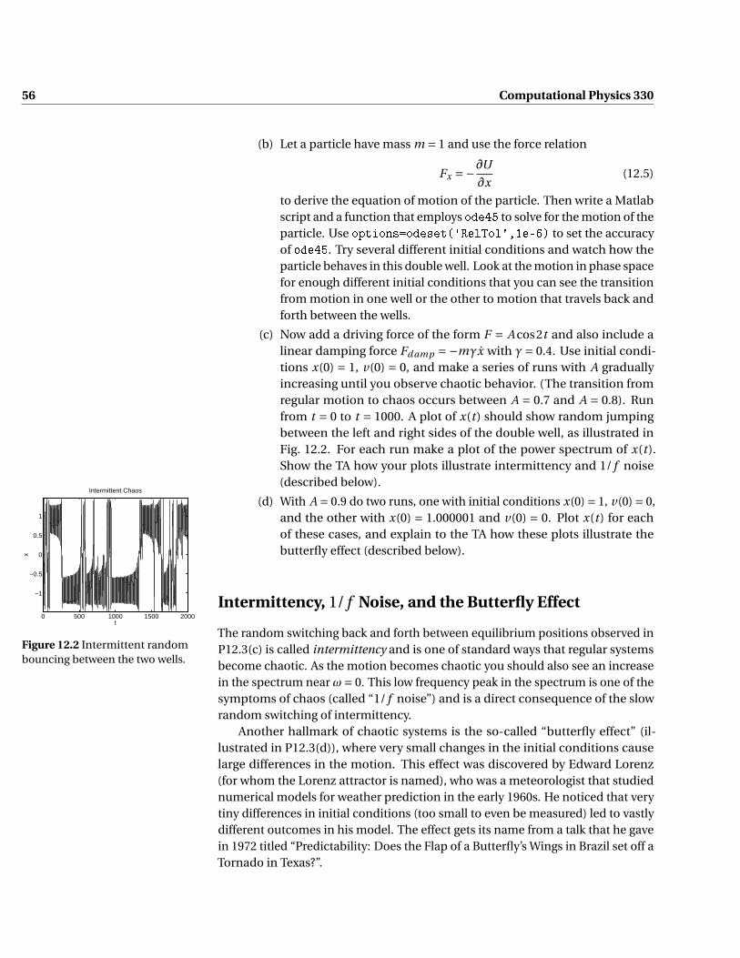
56 Computational Physics 330
(b) Let a particle have mass m = 1 and use the force relation
Fx =−∂U
∂x(12.5)
to derive the equation of motion of the particle. Then write a Matlabscript and a function that employs ode45 to solve for the motion of theparticle. Use options=odeset('RelTol',1e-6) to set the accuracyof ode45. Try several different initial conditions and watch how theparticle behaves in this double well. Look at the motion in phase spacefor enough different initial conditions that you can see the transitionfrom motion in one well or the other to motion that travels back andforth between the wells.
(c) Now add a driving force of the form F = A cos2t and also include alinear damping force Fd amp =−mγx with γ= 0.4. Use initial condi-tions x(0) = 1, v(0) = 0, and make a series of runs with A graduallyincreasing until you observe chaotic behavior. (The transition fromregular motion to chaos occurs between A = 0.7 and A = 0.8). Runfrom t = 0 to t = 1000. A plot of x(t) should show random jumpingbetween the left and right sides of the double well, as illustrated inFig. 12.2. For each run make a plot of the power spectrum of x(t).Show the TA how your plots illustrate intermittency and 1/ f noise(described below).
0 500 1000 1500 2000
−1
−0.5
0
0.5
1
t
x
Intermittent Chaos
Figure 12.2 Intermittent randombouncing between the two wells.
(d) With A = 0.9 do two runs, one with initial conditions x(0) = 1, v(0) = 0,and the other with x(0) = 1.000001 and v(0) = 0. Plot x(t) for eachof these cases, and explain to the TA how these plots illustrate thebutterfly effect (described below).
Intermittency, 1/ f Noise, and the Butterfly Effect
The random switching back and forth between equilibrium positions observed inP12.3(c) is called intermittency and is one of standard ways that regular systemsbecome chaotic. As the motion becomes chaotic you should also see an increasein the spectrum near ω= 0. This low frequency peak in the spectrum is one of thesymptoms of chaos (called “1/ f noise”) and is a direct consequence of the slowrandom switching of intermittency.
Another hallmark of chaotic systems is the so-called “butterfly effect” (il-lustrated in P12.3(d)), where very small changes in the initial conditions causelarge differences in the motion. This effect was discovered by Edward Lorenz(for whom the Lorenz attractor is named), who was a meteorologist that studiednumerical models for weather prediction in the early 1960s. He noticed that verytiny differences in initial conditions (too small to even be measured) led to vastlydifferent outcomes in his model. The effect gets its name from a talk that he gavein 1972 titled “Predictability: Does the Flap of a Butterfly’s Wings in Brazil set off aTornado in Texas?”.

Lab 12 Chaos 57
P12.4 (a) Make a phase space plot for the system in P12.3(c) with A = 0.96. Youshould find that the chaotic behavior quiets down and is replaced bya limit cycle in phase space. It will be difficult to see the limit cycle onthe phase space plot because of the messy transients at the beginning.To eliminate the transients make the phase space plot like this (Wechose to skip the first 60%–you can try your own value):
N=length(x);
n1=ceil(.6*N); % n1 starts 60% into the array
plot(x(n1:N),v(n1:N));
(b) Make another phase space plot at A = 1.30. The single limit cycleshould be replaced by a 2-cycle (two loops in phase space beforerepeating);
Note: to really see the multiple character of these cycles, use the zoomfeature in the plot window to look carefully at them, especially nearthe tight loops. This is shown in Fig. 12.3 for the 4-cycle state. Inthe upper window the full time history is shown from the beginningwhile in the lower window the late-time final state in the windowfrom the upper frame is shown. There are clearly 4 repeated loopsin phase space, so this is called a 4-cycle. This is an example of thefamous “period-doubling route” to chaos, as well as an example ofregular behavior in a region of parameter space where you might haveexpected chaos.
−1.5 −1 −0.5 0 0.5 1 1.5
−1
0
1
x
v
4−cycle
−0.8 −0.75 −0.7 −0.65 −0.6 −0.55 −0.5−0.1
−0.05
0
0.05
x
v
Figure 12.3 Full time history, thenfinal 4-cycle state from the smallwindow. There are fewer loops inthe lower trace because it is thefinal state; the extra loops in thebox in the upper trace are fromearly times.
(c) Make phase space plots of the limit cycle at A = 1.36 (a 4-cycle state),which is then replaced by an 8-cycle at A = 1.371, and then chaostakes over again.
If you run with A = 1.97, 1.99, and 2.0, you will see chaos disappear tobe replaced by a 2-cycle, a 4-cycle, and an 8-cycle. Beyond 2 there ischaos again.
At A = 3 the amplitude is large enough that the oscillator becomesslaved to the drive and we have entrainment. You might think thatlarge A would always cause entrainment, but A = 50 is chaotic, andthere are probably lots of 2,4,8,... cycles and chaotic regions as A isvaried. We ran out of patience; let us know what you find.
Note: when you run with A = 1.36 your phase-space picture may looklike an upside-down left-right flipped version of Fig. 12.3. This is OK–the differential equation is almost unchanged if (x, v) is replaced with(−x,−v). The only difference is that the driving term is replaced byits negative, which is equivalent to a phase shift of π. Such a phaseshift could occur by having the oscillator start up in a different way,which might easily happen if your initial conditions were not exactlythe same as ours. This flipped-over state is to be expected on physicalgrounds. Our picture has tight loops on the left and big loops on theright, but the potential is left-right symmetric; there should be anotherstate with tight loops on the right and big ones on the right as well.

58 Computational Physics 330
Fractals
P12.5 (a) The Fibonacci sequence Fn is defined by
F1 = 1 ; F2 = 1 ; Fn = Fn−1 +Fn−2 for n ≥ 3 (12.6)
(The first few numbers in the sequence are 1,1,2,3,5,8,13, ...). Writea loop that fills the array Fn with the first 100 values of the Fibonaccisequence.
Figure 12.4 The function plottedin P12.5
(b) Now define an array x that goes from −2π to 2π with 50,001 equallyspaced values, like this:
h=4*pi/50000;
x=-2*pi:h:2*pi;
Then write a loop that evaluates the Fourier-like series
G(x) =100∑n=1
cos(Fn x)
Fn. (12.7)
Plot this function vs. x and carefully observe its shape (this functionis shown in Fig. 12.4). Then use the zoom feature to more closelyexamine some of the smaller mountain peaks to discover that eachmountain peak contains smaller versions of itself.
If you zoom in too much you will run out of points, so now plot thefunction again using 50,001 points between x = 3.1 and x = 3.2, andzoom in again. This kind of curve is called a fractal, or fractal curve 2
and such curves are important in chaos theory.
2S. N. Rasband, Chaotic Dynamics of Nonlinear Systems (John Wiley and Sons, New York, 1990),Chap. 4, and http://sprott.physics.wisc.edu/fractals.htm

Lab 13
Coupled Nonlinear Oscillators
When two or more oscillators are hooked together, we say that they are cou-pled. 1 Our final model for driving a swing was an example of coupled pendula.In that case the rotation of the swinger was coupled to the rotation of the overallswing, which allows you to drive the swing.
In this lab we consider a different method for coupling pendula. Consider twopendula hanging from the same piece of horizontally-stretched rubber tubing.If one pendulum is held fixed and the second is displaced from equilibrium, thesecond one experiences a restoring torque from two separate sources: (a) gravityand (b) the rubber tubing. If both pendulums are displaced together each oneexperiences gravity and restoring torque from the tubing, but the tubing betweenthe two plays no role because they both twist it in the same direction. But if thependulums are displaced in opposite directions then the tubing between themis flexed, causing an extra restoring torque. This difference in restoring forcebetween the “together” and “opposite” motions is the cause of the two slightlydifferent frequencies that produce the beating you will see throughout this lab.
Coupled Equations of Motion via Lagrangian Dynamics
For small displacements, the effect of gravity (plus a small contribution from thetubing) can be modeled as restoring torsional springs with spring constants κ1
and κ2 for pendulum 1 and pendulum 2, respectively. This leads to a potentialenergy
U = 1
2κ1θ
21 +
1
2κ2θ
22 . (13.1)
The tubing also adds a coupling term to the potential energy of the form
Uc = 1
2κc (θ1 −θ2)2 (13.2)
Note that this extra restoring potential energy is zero if the angular displacementsare equal. The total potential energy is
U = 1
2κ1θ
21 +
1
2κ2θ
22 +
1
2κc (θ1 −θ2)2 . (13.3)
P13.1 Combine this potential energy function with the kinetic energy
T = 1
2I1θ1
2 + 1
2I2θ2
2(13.4)
1 G. Fowles and G. Cassiday, Analytical Mechanics (Saunders, Fort Worth, 1999), p. 443-460.
59

60 Computational Physics 330
to build the Lagrangian (L = T −U ). Use the Lagrangian equation of motion
∂L
∂qi− d
d t
(∂L
∂qi
)= 0 (13.5)
to derive equations of motion for θ1(t) and θ2(t). Then simplify theseequations by assuming that the two pendula are identical so thatκ1 = κ2 = κand I1 = I2 = I . Also eliminate the spring constants and moments of inertiain favor of frequencies according to the definitions
ω20 =
κ
I; ω2
c =κc
I. (13.6)
Finally, put these two second-order differential equations in coupled firstorder form.
If you did P13.1 correctly, you should have arrived at the following four first-order differential equations for describing the motion of the coupled-pendulumsystem:
θ1 = ω1 (13.7)
θ2 = ω2 (13.8)
ω1 = −ω20θ1 −ω2
c (θ1 −θ2) (13.9)
ω2 = −ω20θ2 −ω2
c (θ2 −θ1). (13.10)
The four variables are: the angular positions of the two pendulums θ1(t) andθ2(t ) (remember that θ = 0 corresponds to the pendulum hanging straight down)and, the angular velocities of the two pendulums ω1(t ) and ω2(t ). The parameterω0 is associated with the natural frequency of a single pendulum without anycoupling, and the parameter ωc is associated with the natural frequency of themiddle section of tubing when attached to the two pendula.
P13.2 (a) Use Mathematica to solve Eqs. (13.7)-(13.10) symbolically withoutinitial conditions to see if you can find the two separate frequenciesthat cause the beating you will see when you solve them in Matlab.
(b) Now numerically solve this system in Matlab with ω0 = 1.3 and ωc =0.3; for initial conditions let everything be zero except θ1(0) = 0.3.Make plots of θ1(t ) and θ2(t ), one above the other using subplot2 likethis:
subplot(2,1,1)
plot(te,th1e)
subplot(2,1,2)
plot(te,th2e)
0 50 100 150 200 250−1
0
1
t
θ 1
Beats
0 50 100 150 200 250−1
0
1
t
θ 2
Figure 13.1 Energy passes backand forth between θ1 and θ2 dueto beating.
Run long enough that something interesting happens, i.e., run at leastlong enough that θ2(t) becomes large, then small again. You should
2For more information about subplots, look it up via help subplot using online help in Matlab.

Lab 13 Coupled Nonlinear Oscillators 61
be looking at the beat plot in Fig. 13.1. This pattern of increasing anddecreasing amplitude in the plots of θ1(t ) and θ2(t ) is an example ofinterference beats caused by the presence of two different frequenciesin the dynamics.
(c) Run the solution out for long enough that when you take the FFT ofθ1(t ) you can see the two peaks in the power spectrum correspondingto the two frequencies whose mixing causes the beats. Verify thatthe beat frequency ωb = 2π/Tb , (where Tb is the time for one of theoscillators to be at maximum amplitude, go to zero amplitude, thencome back to maximum amplitude again) is related to the two peaksin the spectrum ω+ and ω− by
ωb =ω+−ω− . (13.11)
Also verify that the two frequencies you observe in the FFT are the twofrequencies predicted by your Mathematica calculation.
Note: the figure at the beginning of this lab does not have enoughoscillations in it for the FFT to work well. As a general rule, your timeplots should look solid if you want to use the FFT. A maximum timearound 2000 works fine.
(d) Now add a linear damping term to the equation of motion for pendu-lum number 2, start the system with these initial conditions: θ1(0) =0.3, θ1(0) = 0, θ2(0) = 0, θ2(0) = 0. and study the motion of the twooscillators. Use
θ2 =−γθ2 +·· · (13.12)
with γ= 0.07. Look at the plots for θ1(t) and θ2(t) and discuss whathappens to the energy that was initially put into pendulum number 1.
(e) Now drive pendulum number 1 by applying a small negative torqueN1 =−0.3 whenever θ1 is positive and θ1 is negative. You will need
t This driving force is essen-tially the same as the inter-mittent torque you apply tosomeone when you pushthem in a swing.
to use an if statement in the M-file that defines the right-hand sideof your set of differential equations to make this work. This drivingforce is similar to the escapement in a pendulum clock in which amechanical linkage allows the weights to push on the pendulum whenit is at the proper place in its motion. Think about this drive and verifythat it always puts energy into pendulum number 1.
As in part (b), don’t damp pendulum number 1; just keep the dampingin pendulum number 2. Run the code long enough that the systemcomes to a steady state in which both pendulums have constant am-plitude. Discuss the flow of energy in this system.
Coupled Wall Clocks
Now we are ready to study a very famous problem in dynamics. In the 1600sChristian Huygens observed that when two clocks are hung next to each other

62 Computational Physics 330
on a wall, they tend to synchronize with each other. Let’s see if we can make ourequations of motion do this.
P13.3 (a) Begin by making both pendulums be damped and driven as describedin P13.2(d) and (e), but remove the coupling by setting ωc = 0. Runthe code and make sure that each clock comes to its own independentsteady state.
Now add weak coupling between the two by setting ωc = 0.3 again(the slight pushes and pulls that each clock exerts on the wall is thesource of this coupling) and see if the clocks ever synchronize witheach other. (Synchronization means that the two pendulums have thesame period with some definite phase shift between them. This effectis called entrainment in the nonlinear dynamics literature).
When you do these runs, start pendulum 1 with θ1 = 1 and θ1 = 0 andtry various choices for the initial conditions of pendulum number 2.When they become entrained, check the phase difference betweenthe two clocks. (A visual inspection is probably sufficient). In yournumerical experiments, how many different phase relationships doyou observe? (Try overlaid plots of θ1 and θ2 to see the phase relation-ships). Do your in-phase and out-of-phase entrained states have thesame frequencies?
(b) According to the nonlinear dynamics literature, entrainment is aneffect that depends on the oscillators being damped, driven, andnonlinear. Where is the nonlinearity in our equations of motion?
(c) Finally, let’s make these clocks a little more realistic by (i) replacing−ω2θ by −ω2 sinθ in each equation of motion and by (ii) having theirnatural frequencies be slightly different. Do this by changingω2 in theequation of motion for pendulum 2 to 1.03ω2, 1.1ω2, and 1.25ω2 (doall three cases). You should find that entrainment is relatively robust,meaning that the clocks don’t have to have exactly the same period tosynchronize, but that if they are too different the effect is lost. Doesthis robustness depend on the strength of the coupling parameter ωc ?Comment on what your answer to this last question has to do withreal clocks on a wall.
Solving Nonlinear Equations
P13.4 Read and execute the examples in Introduction to Matlab, Chapter 14. Thencomplete the following exercises.
(a) Write a loop that makes an array containing the first 40 zeros of theBessel Function J0(x). Find these zeros by writing a loop to load themusing Matlab’s fzero command. You will have to give fzero a search

Lab 13 Coupled Nonlinear Oscillators 63
range instead of just an initial guess, and this will be easier if youremember that the zeroes of J0(x) are separated by about π.
Look through your list of zeros and make sure that there are no re-peated values. Then plot J0(x) and put a red x at every zero.
(b) Solve the following set of equations using Matlab’s fsolve command
x2 + y2 + z2 = 139x
x + y − z= 3
xp
z = (10− y)2


Index
Amplitude, 23Attractor, 54
Baseball with air, 18Bessel function zeros, 63Butterfly effect, 56
Chaos, 53Coupled oscillators, 59critical damping, 22
Differential equations with Matlab, 53Dynamical chaos, 53, 55
Entrainment, 54, 57, 62Euler’s constant, 11
FFT, 37Fibonacci numbers, 58Fourier transform, 37Fractal curve, 58
Gravitating bodies, 31
harmonic oscilator, 22High-frequency driving forces, 51
Integrals, numerical, 13Intermittency, 56
Limit cycle, 54
Parametric oscillator, 41Pendulum, 27Pendulum period, 28Pendulum, driven, 29Period-doubling route to chaos, 57Phase shift, 23Phase space, 9
Ponderomotive forces, 52Pumping a swing, 41
resonance curve, 24Roundoff, 14
Simple harmonic oscillator, 23Strange attractor, 54
Zeros, Bessel functions, 63
65