picturing the physics behind equations and graphs
TRANSCRIPT

PICTURING THE PHYSICS BEHIND EQUATIONS AND GRAPHS: A GROUNDED
COGNITION BASED MODEL FOR MULTIMEDIA LEARNING AND ITS
APPLICATION IN PHYSICS EDUCATION
BY
ZHONGZHOU CHEN
DISSERTATION
Submitted in partial fulfillment of the requirements
for the degree of Doctor of Philosophy in Physics
in the Graduate College of the
University of Illinois at Urbana-Champaign, 2012
Urbana, Illinois
Doctoral Committee:
Professor Mats Selen, Chair
Professor Gary Gladding, Director of Research
Professor Lance Cooper
Professor Elizabeth Stine-Morrow

ii
ABSTRACT
This thesis tries to answer a fundamental question in physics education: How does the design of
instructional representations affect the process of constructing physics knowledge? This question is
important for the creation of instructional materials of any form, ranging from printed textbooks to
blackboard writings in the classroom. It is especially critical for the creation of computerized multimedia
lectures, as the visualization power of the computer opens up almost limitless possibilities to represent
physics concepts in novel ways.
To answer this question, I bring together knowledge from three different areas: physics education
research (PER), multimedia learning (MML) theory, and most importantly, the perceptual symbols
system (PSS) framework of grounded cognition. I argue that neither the existing PER theories nor the
existing MML models are able to provide a satisfactory answer to this question alone. The reason of
which, I believe, is that these theories are based on an amodal symbol view of cognition.
The PSS framework, however, “grounds” human cognition in “modal symbols”: neural activation of
sensory/motor modals of the brain. By adopting this framework, I have constructed a new cognitive
model for physics learning from multimedia representations that has much greater predictive power
compared to the existing models, especially with respect to the effectiveness of visual representations.
This new model predicts that the perceptual features of instructional representations (graphs, equations
and text), can have a significant impact on students’ learning outcome. If correctly designed, perceptual
features can greatly improve the effectiveness of instructional materials.
We examined the major predictions of the model in two clinical experiments. The results of experiment 1
shows that perceptually enhanced design based on the new model has a positive impact on students’
conceptual understanding, as well as on their ability to transfer the knowledge learned to a different
context. The results of experiment 2 suggest that perceptually enhanced design may also improve
knowledge activation and facilitate the creation of multi-step solutions. However, several other factors not
included in this model may also have a significant impact on the learning outcomes. None of the existing
models of MML are able to account for these results.
In the last chapter, we discuss several factors of the learning process that are not covered in the current
model, and point out several possible directions for future improvements.

iii
To: My Mother and Father

iv
ACKNOWLEDGEMENT
I would like to thank my thesis adviser, Professor Gary Gladding, for his
guidance, support and trust throughout this project. I would like to thank Professor
Jose Mestre, Professor Brian Ross and Professor Tim Stelzer for provocative
discussions and insightful suggestions. Many thanks to Michael Scott who
provided critical technical support for both experimental setup and data collection.

v
Table of Contents
1 Introduction ........................................................................................................................................... 1
2 Cognitive Theories of PER ................................................................................................................. 12
2.1 The misconceptions view: ........................................................................................................... 13
2.2 The Knowledge in Pieces View: ................................................................................................. 14
2.3 The Ontological Categorization View: ....................................................................................... 19
2.4 Summary ..................................................................................................................................... 21
3 Multimedia Learning Theories ............................................................................................................ 23
3.1 Multimedia Learning theory of Richard Mayer .......................................................................... 23
3.2 Multimedia Learning Model by Schnotz .................................................................................... 28
3.3 Common Difficulties Facing Existing Theories of Multimedia Learning .................................. 32
4 The Perceptual Symbols System Framework of Grounded Cognition ............................................... 35
4.1 Perceptual Symbols ..................................................................................................................... 35
4.2 Simulations: ................................................................................................................................ 38
4.3 Concepts ...................................................................................................................................... 40
5 The Process of Learning from a Grounded Cognition Perspective ..................................................... 42
5.1 A grounded cognition definition of learning ............................................................................... 42
5.2 The Symbolic Method ................................................................................................................. 42
5.3 The Perceptual Method ............................................................................................................... 44
5.4 The Categorical Inferences Method ............................................................................................ 47
5.5 Final Remarks ............................................................................................................................. 49
6 A Grounded Cognition Based Multimedia Learning Model ............................................................... 51
6.1 The Model ................................................................................................................................... 51
6.2 The impact of instructional material design on problem solving ................................................ 65
7 Experiment 1 ....................................................................................................................................... 70
7.1 Multimedia Design and Predictions ............................................................................................ 70
7.2 Methods and Implementation...................................................................................................... 78
7.3 Experiment 1 Results .................................................................................................................. 81
7.4 Discussion ................................................................................................................................... 91

vi
8 Experiment 2 ....................................................................................................................................... 99
8.1 Multimedia Design and Predictions ............................................................................................ 99
8.2 Methods and Implementation.................................................................................................... 107
8.3 Results ....................................................................................................................................... 109
8.4 Discussion ................................................................................................................................. 117
9 Summary ........................................................................................................................................... 123
10 Limitations and Future Directions ................................................................................................ 126
Reference: ................................................................................................................................................. 129
Appendix A: Experiment 1 Pretest ........................................................................................................... 136
Appendix B: Experiment 1 Posttest .......................................................................................................... 137
Appendix C: Experiment 1 Posttest Detailed Grading from each grader ................................................. 145
Appendix D: Experiment 2 Pretest ........................................................................................................... 146
Appendix E: Experiment 2 Posttest .......................................................................................................... 148

1
1 Introduction
In his 2007 article to the American Physical Society(C. Wieman, 2007), Carl Wieman described
in detail the so called “curse of knowledge”: the more expertise one gains in any field, the less likely he is
able to convey that expertise to a novice. This peculiar nature of the human mind is all too familiar to us
as physics teachers, as our well prepared, crystal clear lectures are often greeted with students’ blank
faces and confused expressions; our carefully designed, powerful computer simulations frequently result
in little if any learning gains. As Wieman puts it “…it is almost as if the instructor and the student are
speaking different languages but neither realizes it”.
Among the many possible ways to understand this strange phenomenon, the one that I found most
intriguing comes from an idea expressed in a 1979 book chapter by Michael Reddy(Reddy, 1979), called
the “conduit metaphor”1. Reddy argues that most of us involuntarily think of language as a conduit, which
we could “put our thoughts into”, and others could “get the meaning out of”.
When it comes to teaching physics, we often naturally assume that our physics knowledge is
contained within the equations we write, the graphs we draw, and the explanations we give to students.
Upon receiving the graphs and equations, students should have received the physics knowledge contained
in them. Therefore, their learning difficulties are either caused by them not spending enough effort to
“extract” what was received or us forgetting to “load” enough knowledge into our representation.
Of course, knowledge can neither be contained in language nor transferred from one brain to
another. Knowledge, which is by nature connection patterns of neurons, is strictly confined within the
brain itself. The equations and graphs we put down could be seen as traces and marks left behind due to
the thought process involving our physics knowledge. Upon receiving these traces, the receiver has to
reconstruct, with whatever mental resource he possesses within his own brain, a thought process that is
similar enough to that of the sender’s, according to what he has received. 2
Apparently, the more similar the knowledge backgrounds are between sender and receiver, the
more likely it is for the regeneration to be successful. Chess grandmasters are able to reconstruct chess
1 Reddy’s discussion is based on the English language and limited to English speakers. As a native Chinese, I think the same idea
applies perfectly to Chinese speakers as well. 2 The idea of constructivism has been around for quite a long time. However, Reddy demonstrated how easily it is (sometimes
even inevitably) for us to slip back into the conduit metaphor.

2
positions taken from grandmaster games by a quick glance at the board, while the same position would be
almost impossible for a novice to remember(Chase & Simon, 1973). 3
However, the knowledge background between instructor and student couldn’t be more different.
Therefore, an instructor who does not deliberately take into account what his students are capable of
reconstructing, could easily end up generating knowledge representations that sound like a foreign
language to his students, even though the equations and explanations appears to himself as being crystal
clear and beautifully written. In fact, the feeling of them being clear and beautiful is a result of his own
physics knowledge in the background; and if he happens to have slipped into the “conduit metaphor”,
which is almost inevitable according to Reddy, he would have thought that the clarity and beauty of the
equations should have also reached his students together with the equations.
To make matters worse, in most cases it is not that the instructor is unwilling to consider what his
students are capable of reconstructing, but rather that he is unable to do so. It has been shown that it can
be extremely hard, if not totally impossible, for an expert mind to think intuitively from the perspective of
a novice. The chess grand masters who were able to memorize the game positions of other grand masters
in a blink of an eye had considerable difficulty reconstructing game positions played by novices, which
they report to be “unreasonable”. 4 Experienced physics instructors who are well aware of the “curse of
knowledge”, even Carl Wieman himself, are constantly surprised at the way their students perceive and
interpret their knowledge representations(C. E. Wieman & Perkins, 2006).
How then, could we learn to “speak the language” of our students, and design our instructional
materials so that they can be easily interpreted by our students?
When our intuitions fail us, we have to rely on knowledge to serve as our dictionary of “students’
language”. Knowledge of how the novice mind comprehends and learns from representations, which
would allow us to look beyond our “cursed” intuitions, and present physics in ways that we would never
have thought of before.
It may seem that the first thing we need is a “catalogue” of the resources, especially physics
resources, possessed by our students, with which they are able to reconstruct meaning. However, the
catalogue wouldn’t be of much use to us if it consists entirely of factual statements such as: “know how
to calculate electric potential using the equation”, “have difficulty with conductors”, or “cannot determine
the limits of this integral”.
3 Grandmasters and novices have no difference in memorizing random chess positions, so this is not caused by a
difference in memory capacity. 4 In fact, chess players of all levels are shown to have best memories for games of their own level.

3
Knowing that students have difficulties with conductors does not explain why our attempts to
teach the properties of conductors consistently fail. We would like to know why, after telling our students
“electric potential stays the same inside a conductor” for so many times, a significant number of them still
often treat the electric potential as zero.
Therefore, what we really need is a finer grained theoretical frame work with which to describe
the underlying structure of concepts. We would like to find out what “ingredients” students add to their
understanding of concepts such as “electric potential”, “stays the same” and “conductor”, so that we could
identify which ingredient(s) went wrong.
Such theoretical frameworks have already been developed to some extent, in the field of physics
education research (PER)(Docktor, 2010).
For example, some researchers (DiSessa, 1993; Hammer, 2000) hypothesize that bigger concepts
are made of “miniature pieces of thought”, called phenomenological primitives (p-prims). P-prims are
small basic units of ideas that are used without further explanation during a reasoning process. For
example, the p-prim of “more is more”, is often used by students in reasoning about a number of physics
concepts, either correctly or incorrectly, such as “a larger capacitor stores more charges” and “heavier
objects fall faster”.
Others have proposed that a body of smaller pieces of knowledge is organized under a single
general category, such as an “object” or a “process”(M. T. H. Chi & Slotta, 1993; Gupta, Hammer, &
Redish, 2010; Slotta, Chi, & Joram, 1995). If students happen to think of force as an “object”, then the
body of knowledge associated with the “object” category, such as “can be used up” and “can be divided”,
are used to reason about force. As a result, students would generate arguments such as “an object slows
down when the initial pushing force is used up”, or “force is divided between two blocks traveling
together”.
These theories provide novel ways of understanding students’ difficulties with physics concepts,
and they have inspired a number of new interventions. However, there still exist plenty of details in each
of these theories that require further explanation. For example, how does the students’ brain learn to
activate the appropriate p-prim to reason about a certain concept? Why are some physics entities, such as
electric potential, much harder to be correctly categorized than other entities such as electric charge? As
we shall see in the next chapter, we are still in short supply of proper tools that would allow us to
effectively reshape students’ knowledge structure

4
Aside from a “mental resource catalogue”, it is also important for us to know how to efficiently
and accurately activate the intended mental resources in the students mind. In other words, what equations,
graphs and demonstrations should we give our students, so that the right mental “building blocks” are
being brought to their mind, and are combined correctly to form the idea that we want to teach them?
As a simple example, if we wish to activate the resource of the color yellow, reading the word
“yellow” certainly requires much less processing and is less error prone than reading “electromagnetic
wave of approximate wavelength 570nm ”, but how does it compare to seeing a patch of yellow color?
How should we represent abstract physics ideas, such as ‘electric potential is the accumulation of electric
field over space’, that lacks both an apparent visual appearance, and proper descriptive language that is
easy to understand by students?
The question of how knowledge is constructed based on various forms of representations is by
definition the core focus of research in multimedia learning (MML). However, as is reviewed in chapter 0,
current multimedia learning theories are unable to answer many of the questions that we are interested in.
Current multimedia learning theories (Mayer, 2001; Reed, 2006; Schnotz, 2003) describe in detail
how the brain allocates different types of memory resources, such as visual working memory and verbal
working memory, to process visual and verbal signals. It provides principles for designing multimedia
instruction representations that efficiently utilize the limited capacity of these memory systems, so that
the brain is not overwhelmed by a single type of signal at any time.
However, avoiding memory overload is certainly not the solution to all our problems in teaching.
In physics, even some of the easiest representations, such as the acceleration vs. time graph, has a high
chance of being misinterpreted by students(Kozhevnikov, Motes, & Hegarty, 2007; Trowbridge &
McDermott, 1981). Processing such an easy graph should be well within the visual memory capacity of
any college student. Apparently, the problem here is not caused by insufficient memory resources, but
rather by the knowledge construction process taking place inside these memory resources.
Unfortunately, neither of the theoretical models reviewed in chapter 0 present a satisfactory
description of how the brain constructs new knowledge based on external signals received. A direct result
of missing such a description is that neither theory is able to judge the quality of an individual
representation from a knowledge construction perspective, less providing suggestions for improvements5.
In other words, the theories couldn’t inform an instructor in advance whether his drawing of
5 The theoretical model by Schnotz is able to judge the usefulness of diagrams in a limited number of cases.
However, it is only applicable to cases where the exact same diagram could be used for a number of problems, which is fairly uncommon in physics.

5
electromagnetic field might be confusing to students, nor would it be able to provide any useful
suggestions as to improving the drawing.
Not surprisingly, according to both our own experience (Chen, Stelzer, & Gladding, 2010) and
published research from other groups(Byrne, Catrambone, & Stasko, 1999), multimedia instructional
materials created for sophisticated domains such as physics and computer science, designed based on
existing principles of MML , have had mixed results in learning gains ranging from significant
improvements to even negative effects.
Therefore, in order for us to more productively apply MML theories to the teaching of physics,
we must first fill in the missing details of the knowledge construction process.
Upon closer examination, it is easy to notice that the missing pieces from PER and MML have
much in common. Specifically, PER provides a description of students’ internal knowledge structure, but
is unable to relate it to perceived external representations. On the other hand, MML models outlined the
process of comprehending perceivable representations, but are vague on what kind of knowledge structure
is constructed from the comprehension. Missing from both disciplines is a satisfactory link between
external knowledge representations, such as graphs and equations, and internal knowledge representations
such as p-prims and concept categories.
Missing such a link in both theories left us in a rather awkward situation. From a PER perspective,
we know a lot about students’ misunderstandings, but don’t know for sure what to do about it. From the
MML perspective, we are able to make instructions easy for students to understand, but don’t know what
kind of understanding would result from the instructions.
We believe that the cause of this problem lies in the way we understand the nature of knowledge.
For the past 30 years, mainstream cognitive psychologists believe that the brain represents knowledge in
the form of “amodal symbols”: abstract symbols that are being processed by specialized neural circuits of
the brain, independent of all the sensory/motor systems. For example, upon seeing a chair, the brain
translates the perception into a “chair” symbol (bearing no resemblance to the perceived chair), which is
linked to other features such as “back”, “leg” or “sit” through propositional relations such as HAS(CHAIR,
BACK), and SIT(PERSON, CHAIR). If the brain could be viewed as a computer, then the “amodal
symbols” are its “0”s and “1”s that are computed by its specialized CPU. Sensory/motor systems on the
other hand, function much like the graphics card and the sound card, which are responsible for translating
back and forth between amodal symbols and perception of images, sounds, movements and emotions.
6
Such an amodal symbol approach is adopted, either implicitly or explicitly, by theories from both PER
and MML.
However, one of the most prominent challenges facing the amodal symbol view of knowledge, is
that a satisfactory explanation of how these symbols arise from, and feed back into the sensory/motor
systems has never been found (Lawrence W. Barsalou, 1999). Even after 30 years of research, these
mysterious symbols still lie in a black box within the brain, impenetrable by all of our senses. Therefore,
it is no surprise that both PER and MML theories adopting this view of knowledge are having a hard time
linking external representations to internal knowledge structures.
Recently in cognitive psychology, there has been an increasing amount of skepticism on the
validity of amodal symbols(Lawrence W. Barsalou, 2008, 2010). Motivated by a number of intrinsic
difficulties faced by the amodal symbol view (including the one mentioned above), and supported by
accumulating neuro-imagery evidence, a number of researchers such as Barsalou are starting to argue that
amodal symbols are the “ether” of human cognition.
Stemming from their research is a new branch of cognitive psychology called grounded cognition.
The central idea behind grounded cognition is that all of peoples’ knowledge and cognition are being
stored and carried out (or ‘grounded’) in the sensory/motor domains of the brain. According to
researchers in grounded cognition, evolution has enabled the human brain to cleverly utilize existing
neural circuits in sensory/motor domains, to perform more advanced cognitive tasks such as abstract
reasoning and language comprehension. (Anderson, 2007; Lawrence W. Barsalou, 1999)
Under the framework of grounded cognition, the connection between perceived representation
and internal knowledge structure almost “rides for free”, since they are written in the same “language”,
and processed by much of the same domains in the brain6. What is left for us to do is to rewrite both the
knowledge structures of PER and the knowledge construction process of MML in terms of activation of
sensory motor domains, under the framework of grounded cognition, in much the same way as rewriting a
physics problem in terms of math. Just as solving math equations leads us to new physics insights,
rewriting (and combining) PER and MML theories under grounded cognition will provide us with new
principles to guide the design of effective instruction.
In the following chapters, we will first review the results and limitations of current PER and
MML theories, followed by a brief introduction to the “perceptual symbols system” theoretical
6 With the exception of language comprehension

7
framework developed by Barsalou. We will also demonstrate that the various knowledge structures
proposed by PER theories could all be included under the grounded cognition framework.
We will then revisit MML learning theories, and show how understanding multimedia learning
from a grounded cognition perspective could lead us to a new theoretical model, which has significant
structural differences with the existing models reviewed in the previous chapter.
By combining the new MML framework with the new physics knowledge structure, we are able
to obtain some new insights for physics instruction. Namely, the biggest potential power of computer
animation is not that it can provide more “information”, but rather it is able to provide extra visual
perception compared to static figures. Visual perception, when properly integrated into instruction, will be
able to 1) facilitate knowledge transfer between different contexts and 2) improve the recall of proper
knowledge during certain types of problem solving.
In the second part of this thesis, we will try to provide evidence for those two theoretical
predictions through two clinical experiments.
Experiment one explores whether providing proper visual perception could improve students’
understanding of a worked out solution to an example problem, and then transfer this understanding to a
new problem with very different surface features.
In this experiment, we created three different versions of multimedia solutions to two difficult
problems involving the calculation of electric potential in space by properly integrating the electric field
(Figure 1). Version 1 and 3 are designed as controls, and version 2 contains proper visual perceptions
according to grounded cognition principles.
All three versions of the solution take the form of a piece of audio narration accompanied by
visual animation. Version 2 and 3 contain exactly the same audio narration, while version 1’s narration
contains some trivial differences that will become obvious below.
The accompanying animation in version 1 is designed to mimic the illustration that could be
created by any experienced instructor or teaching assistant, when explaining the problem to a student in
detail. In version 2, a visual sense of “accumulation” is created by displaying colored equipotential lines
appearing one by one, when the audio script talks about the integration of electric field. Although the
color and thickness of equipotential lines roughly resemble the relative magnitude of electric potential in
space, it was never mentioned in the audio narration. In version 1, the integration process is illustrated by
a straight line going through a series of points, which leads to the slight difference in audio narration.

8
Version 3 also contains equipotential lines, but the lines are drawn in black with equal thickness, and
remain static throughout the narration, completely eliminating the visual sense of “accumulation”, while
keeping all the spatial relations exactly the same.
Figure 1: : Snapshot of three different versions of animation showing the integral of electric field from experiment one: a)
version 1 mimics the drawing by a teacher on blackboard b) version 2 provides perception of accumulating electric
potential c) version 3 uses uniform black equipotential lines which conveys the same spatial relation but no perception.
Since the three versions are only different in details of visual representation design, they all
comply with existing multimedia design principles to the exact same degree. Moreover, electric potential
is an abstract concept with no “look”. Unlike mechanical devices such as pumps and ratchets (Mayer &
Anderson, 1991; Schwartz & Black, 1996), it does not require explicit mental imagery to reason about.
Therefore, according to some researchers (Byrne et al., 1999; Mireille Betrancourt, 2005), animation
should have only a limited effect on understanding this type of abstract concept.
Strictly speaking, since version 2 contains many more visual elements (color, thickness) than the
other two versions, while the explicit meaning of these visual element are not explained verbally, it
should require the most amount of visual cognitive capacity to process, which means that there’s a high
probability of cognitive overload. Therefore, current multimedia learning theories would predict that
version 2 would actually impede learning in low ability students.
However, looking at the problem from a grounded cognition perspective would result in
predictions in the opposite direction. According to grounded cognition (Lawrence W. Barsalou, Ava,
Simmons, & Wilson, 2008; Zwaan & Madden, 2005), deep semantic meanings of words are processed
through the sensory/motor domains of the brain. Abstract concepts are understood via (unconsciously)
mentally simulating one or more situations relevant to the concept(Lawrence W. Barsalou & Wiemer-
Hastings, 2005). In this case, students’ difficulty in understanding the integral expression of the electric
potential is caused by the fact that a situated mental simulation of the accumulation process is very hard to
generate. The conventional ways of depicting the integral process contains no sense of accumulation,
c) b) a)

9
which interferes with neural circuits in visual and other domains of the brain trying to generate the mental
simulation corresponding to the accumulation idea.
According to grounded cognition, the visual sense of “accumulation” in version 2 would
significantly help students in understanding the idea that electric potential difference is the accumulation
of electric field along a certain path. On the other hand, students who studied the other two versions of the
solution would have significant difficulty understanding this idea, and are more likely to interpret the
verbal explanation superficially. Consequently, when faced with a new problem with a different context
but testing the same underlying principle, these students are more likely to generate an incorrect answer
that is superficially similar to the one they’ve learned.
The second experiment is aimed at testing whether providing a perceptual basis for conceptual
understanding would enhance the chance of proper knowledge being recalled for problem solving,
especially for problems that should be solved by execution of multiple explicit rules.
In this experiment, we designed a short piece of multimedia instruction, also in the form of audio
narration accompanied by visual animation. In the instruction, seven explicit rules for calculating the
capacitance, charge and voltage of series and parallel capacitor circuits are introduced in detail. Every
problem students received in the post test can be solved by implementing two or more of these seven rules
in series.
Two different versions of animation are created to accompany the same piece of audio narration
(Figure 2). Version 1 again mimics the drawing that would be created by an experienced teacher in class.
Version 2 schematically represents the charge stored in capacitor by the number of charge icons,
represents the capacitance of each capacitor with their physical sizes, and represents the relative voltage
in different branches of the circuit with different colors and thickness. None of the representations are
explicitly stated in the audio script.

10
Figure 2: Snapshot of two versions of animations in experiment two: a) version 1 mimics the drawing of a teacher on
blackboard b) version 2 represents charge, voltage and capacitance perceptually.
According to the amodal symbol view of knowledge, explicit rules such as “voltage of series
capacitors are inversely proportional to their capacitance” are exclusively coded in propositions and
semantics without doubt. Therefore, these rules should be conveyed predominantly through the verbal
channel, since amodal symbols are thought to closely resemble word forms. (Lawrence W. Barsalou,
1999)
Hence, current multimedia learning theories would once again predict that the added animations
should have little effect on student’s learning, if not being distractive, and should have absolutely no
effect at all when it comes to recalling and implementing these rules for problem solving.
Grounded cognition, on the other hand, rejects the view of the human brain being a rule executing
machine. From an evolution point of view, the ability of understanding language and abstract rules is the
latest addition to the human brain, which makes it hard to believe that it has become the core of brain
functions. Rather, the brain should be extremely fine tuned towards processing and organizing senses and
body movements, since the sensory/motor domains have been evolving ever since the existence of the
brain as an organ.
Hence, implementing abstract rules stored in the form of language should be a rather challenging
and unfamiliar task for the brain. In contrast, it is much more powerful at processing rules when they
come with a concrete perceptual basis.
In addition, language forms alone could not carry any meaning, but rather serve as pointers to
semantic meanings in the brain. Grounded cognition views language as an index for activating
corresponding neural circuits in the sensory/motor domains. In other words, the comprehension of an
abstract verbal rule still needs to be carried out in the sensory/motor domains. Therefore, a rule that is
stored in language form needs to be first “grounded” in perception when recalled, before it could be used
a) b)

11
for reasoning. In comparison, recalling a rule stored perceptually requires no extra translation process,
and therefore should be much more efficient to use.
In conclusion, grounded cognition predicts that students who learned the rules with proper
perception are able to recall and think about these rules much more efficiently, which means that they
could think about and evaluate more rules at any given step, as well as foreseeing more steps ahead,
leading to better decisions in problem solving.
We will show that our experimental results provide strong evidence for the grounded cognition
predictions. Significant effects could be observed even in groups of about 15 subjects.

12
2 Cognitive Theories of PER
In this chapter we will review three major theoretical viewpoints on understanding students’
physics reasoning within the field of PER: the misconceptions view, the knowledge in pieces view, and
the ontological categorization view. All three views try to explain the cause of students’ difficulties with
understanding and reasoning about physics concepts, building on more fundamental cognitive processes.
Based on these explanations, each view suggests its own teaching strategies for treating the difficulties.
To better illustrate the theoretical constructs, we’ll use as an example a particular student
difficulty frequently observed while teaching calculus based introductory electricity and magnetism. The
same topic is later developed into our first experiment in this thesis.
We observed in our E&M class that whenever a problem asks about electric potential in space,
the majority of students consistently prefer using the simple relation of kQ/r, over the integral expression
of∫– , regardless of the context of the problem.
For example, in the following case illustrated in Figure 3, a charge Q is enclosed at the center of
a neutral conducting shell. When asked to calculate the potential difference between points A and B,
students tend to use kQ(1/RB- 1/RA), rather than integrating the E-field from B to A, and skipping the part
inside the shell. When asked to reason about whether changing the thickness or the position of the shell
would affect the potential difference, many students answered that it wouldn’t, since the electric field at
the two points stay the same, or because neither Q nor Rb or Ra has changed.
In addition, when explicitly asked to use the integral expression, many students do not exclude
the part that is inside the conductor.
Figure 3: A point charge Q enclosed by a thick conducting shell shown in gray.

13
In the following, we will demonstrate how this student difficulty could be explained using ideas
from the three different views, and what teaching strategy might each of these views suggest. More
importantly, we’ll also discuss the challenges and limitations faced by each view.
2.1 The misconceptions view:
The misconception view dates back to the 1980s, when it was first proposed by researchers such
as Posner, Clement and McDermott.(J Clement, 1982; Etkina, Mestre, & O’Donnell, 2005; McDermott,
1984; Posner, Strike, Hewson, & Gertzog, 1982)
This view suggests that, before coming into the classroom, students have already gained much
experience with the physical world in which they live. Based on these experiences, they form naïve
explanations of the physical world, such as heavier objects fall faster and exert more force, that are almost
always very different from canonical, scientific understanding. These naïve explanations, or so called
“misconceptions”, are found to be particularly resistant to change. For example, ideas such as heavier
objects fall faster than lighter objects are often found to persist even after college education.
In our case of electric potential, however, it is not obvious what type of everyday experience
might have contributed to the student difficulty, since the concept of electric potential is hardly ever
encountered in everyday life. However, almost all of us have had experience of measuring or calculating
other quantities, such as height, weight, density, speed, and force. All of these values are “local”: the
weight of an object doesn’t depend on other objects nearby, and the height of an object would not depend
on whether it is enclosed by a shell. Students might have treated electric potential as another localized
value, which would explain some of the observed difficulties.
According to the work of Posner and colleagues(Posner et al., 1982; Strike & Posner, 1982),
changing a misconception generally involves four steps: 1) Dissatisfaction with current concept, 2)
Intelligibility of the new concept, 3) Initial plausibility of new concept, and 4) Usefulness of new concept.
In order to create the sense of dissatisfaction, we will need to confront the misconception, which could be
achieved by creating problems in which using the kQ/r equation would result in answers that either
conflict with common sense or are different from experimental observation. This process needs to be
repeated until the dissatisfaction accumulates to the degree that students are willing to give up their naive
understanding. At that point, we can then demonstrate how using the integral equation would provide a
more reasonable result, and hope that at that point students will learn to appreciate it.
Among the three viewpoints, the misconception view is least compatible with the current work
for the following reasons. First of all, it assumes that misconceptions originate from experience with the
14
physical world before formal instruction. Such an assumption in some way implies that misconceptions
are almost inevitable among novices, and instruction could only correct it instead of preventing it.
However, as is discussed in the introductory section, we have reasons to believe that ineffective design of
instruction could be held accountable for at least part of students’ difficulties with physics.
In addition, misconceptions are described as “resistant to change”. Therefore, whenever an
intervention fails to show any effect, it could always be attributed to the resilient nature of misconception
itself, leaving little room for improving the effectiveness of the instruction design. Moreover, the origin of
such “resistance” is attributed to students’ unwillingness to give up their misconception, instead of them
being unable to properly interpret new material. Therefore, the intervention suggested by the
misconception view is focused on creating dissatisfaction for the misconception and showing the
usefulness of the correct conception. The underlying assumption seems to be that the instructor’s
presentation of the correct concept is flawless, and the reason why students don’t learn is because they’re
not thinking hard enough, which is in sharp contradiction with the “curse of knowledge” viewpoint
expressed in the introduction section.
Because of these reasons, in the rest of this thesis we will not incorporate the misconception view
in our theoretical construct. This does not mean that all the ideas of misconceptions view are being
abolished. Instead, some of its core observations are being shared by the other two views. As we will see,
the knowledge in pieces view also acknowledges that students bring a large body of everyday life
knowledge into the classroom. The observation that some students’ conceptions are particularly resistant
to change appears in the ontological categorization view as well.
2.2 The Knowledge in Pieces View:
2.2.1 Overview
As is discussed above, while the intervention suggested by the misconceptions view serves to
create the impetus for initiating conceptual change, it provides little or no scaffolding for making the
changes. Aside from the fact that the student’s “unwillingness to change” is considered as a dominant
factor, the theoretical construct of the misconceptions view also makes it difficult for designing effective
scaffolding.
The misconceptions view treats physics concepts holistically as the basic unit of students’
reasoning, which could only be judged as either right or wrong. While a wrong concept could be
discarded due to dissatisfaction, a right concept cannot be directly placed into the mind. Rather, it has to
be constructed from other things that are already understood (for example English).

15
Apparently, a holistic view of the concept provides little insight on the construction process, and
therefore cannot provide guidance for the designing of appropriate scaffolding that facilitates the process.
In order to do that, we need to know what cognitive “electrons” “protons” and “neutrons” resides beneath
the surface of the “concept atom”.
Researchers holding the knowledge in pieces view, such as David Hammer and Andrea Disessa,
refer to these “basic particles” that compose a concept as “resources”(DiSessa, 1993; Hammer, 1996,
2000; Smith III, diSessa, & Roschelle, 1994). Hammer’s own explanation of “resources” draws on a
similar metaphor:
“This use of the word ‘‘resource’’ derives loosely from the notion of a
resource in computer science, a chunk of computer code that can be
incorporated into programs to perform some function. Programmers virtually
never write their programs from scratch. Rather, they draw on a rich store of
routines and subroutines, procedures of various sizes and functions.”
For example, a frequently mentioned resource is the idea of “closer is stronger”, which is used by people
to make sense of a number of phenomena, from “light is more intense closer to the bulb” to the inverse
square law of gravity.
Past experience with the physical world is the largest source of cognitive resources. The
knowledge in pieces view treats these resources as potential building blocks of a new concept, rather than
obstacles that need to be confronted. A resource such as the idea of “closer is stronger” cannot be simply
judged as being “right” or “wrong”, instead, what really matters is whether it is correctly activated to
reason about a certain concept.
An important claim of the knowledge in pieces view is that the resources a novice activates to
reason about a certain concept is highly context dependent and inconsistent. For example, Steinberg and
Sabella(Steinberg & Sabella, 1997) have found that students’ answers to problems on Newton’s law could
change significantly, depending on the problem’s context (elevator going up vs. platform going down)
and the situation (exam vs. classroom discussion). In addition, Hammer(Hammer, 1996) noticed that
students could put forward both (seemingly) correct and incorrect arguments in the same discussion about
the same concept.
Back to the example of electric potential, a possible explanation of the observed difficulty from
the knowledge in pieces perspective would be that the context of the problem activates the knowledge
piece of “localized value” among students. While this explanation may seem very similar to the one given

16
by the misconceptions view, the two views differ drastically in the suggested intervention to resolve this
difficulty.
The knowledge in pieces view would probably argue that, although the “localized value” resource
seems to be activated quite often, it is neither stable nor resilient to change. On the other hand, students do
possess other resources that could be used productively for correct reasoning. For example, every student
knows that the total number of tolls paid for driving on a segment of a toll road depends on the density of
the toll stations on the road. Therefore, avoiding part of the toll road will result in paying less toll, which
means the “money difference” between the start and end of the trip becomes smaller.
The knowledge in pieces view suggests that intervention should focus on creating a context in
which it is easier for students to activate productive resources. One possible way of doing so involves a
series of scaffolding analogies.(John Clement, Brown, & Zietsman, 1989; Hammer, 1996; Podolefsky &
Finkelstein, 2007) For example, students may first be asked to compare the similarity between paying toll
on a highway and the work done moving a particle through electric field. Then they move from a particle
with a certain charge, to a particle with unit charge, and eventually arriving at the integral for electric
potential. With each analogy, certain key resources are transferred from one context to another, and
finally becoming the building block of electric potential.
To this point, we have used the term “resources” to loosely refer to any small piece of an idea that
seems intuitively less sophisticated than a concept. Apparently, more precise definitions of what counts as
a “resource” is indispensible for constructing a theory of physics learning. To date, several different types
of “resources” have been proposed (DiSessa, 1993; Hammer, Elby, Scherr, & Redish, 2005; diSessa,
1998). Here, we will briefly review as an example the most well-known type of resource:
phenomenological primitives (p-prim).
2.2.2 P-prim as cognitive resource
P-prims are thought to be the smallest units of thought that require no further explanation. The
concept of p-prim was first introduced by Andy Disessa as “base level of our intuitive explanations of
physical phenomena”. (DiSessa, 1993; Sherin, 2006)They are “phenomenological” in the sense that they
are often interpretations of perceptual experiences. A typical example of a p-prim is “closer is stronger”,
which relates two experiences, “closer” and “stronger”. P-prims function by being “recognized”, or
“activated”. They are “primitive” in that their activation is usually intuitive, requiring no further
explanation. They may form the basis of more a complicated explanation, but the validity of themselves
often cannot be explained by the person’s own knowledge system.

17
For example, when feeling cold, one would definitely move towards a nearby camp fire instead of moving
away from it, without thinking about verifying if the relation between radiation power and distance
actually obeys an inverse square law. An (incomplete) list of p-prims identified by diSessa is presented in
Table 1.
P-prim Definition Example usage
Ohm’s p-prim An agent that is the locus of an impetus that acts
against a resistance to produce some sort of result.
One pushes harder to move
heavy objects, which "resist"
motion more.
Resistance Spontaneous resistance to force and influence. A wall does not “push back”,
but rather “resist” pushing.
Force as a mover Pushing an object from rest causes it to move in the
direction of the push
Dying
away/warming
up
The force on an object being
tossed takes time to die away,
and it also takes time for the
object to get up to full speed
(warm up)
Table 1: A sample list of p-prims identified by Disessa(DiSessa, 1993).
In our example of electric potential, part of the difficulty in the use of the integral expression for
potential difference might be explained by students being unable to activate the P-prim called “more is
more”. More precisely, this p-prim takes the form of “more A leads to more B”, in which A and B could
be any two related phenomenon, for example, “the harder you push the faster it moves”, or “the longer
you cook the hotter the food becomes”. In the case of electric potential, the “more is more” p-prim, if
activated, would enable such reasoning as “the more distance accumulated over an E-field, the larger the
potential difference”, or “the stronger the E-field being activated, the larger the total potential difference”
2.2.3 Limitations of knowledge in pieces view
The knowledge in pieces view provides a detailed explanation of students’ difficulties based on
the activation of cognitive resources. What remains unanswered, however, is how the brain determines

18
the proper resources to activate based on perceived external representations, and how such ability can be
acquired through instruction.
Resources such as P-prims do not have a definite one to one correspondence with external
representations such as words and images. We know from experience in teaching that enforcing students
to memorize the sentence “electric potential is the accumulation of electric field, not an object created by
the local field” has very little, if any effect at all, on properly activating the “accumulation” resource
instead of the “localized value” resource for solving problems involving the concept of electric potential.
Nor is it obvious what kinds of graphical representation should be used to represent a particular p-
prim, since resources are defined as cognitive structures abstracted from various previous experiences,
which shouldn’t have a specific visual appearance.
Moreover, activation of resources depends heavily on background knowledge as well as context.
Representation that is generated by an expert according to the activated resource in his mind often results
in activating a completely different set of resources in the student’s mind due to difference in their
knowledge background.
The “scaffolding analogy”/ “bridging analogy” method mentioned above tries to resolve this
problem by placing the instructor and the student in a context in which both have similar expertise, for
example, everyday life experience. Under such a context, the instructor and student have a better chance
of activating a similar set of resources via the same representation, and the instructor could then guide the
student to transfer some of that resource to the unfamiliar physics context.
However, finding an appropriate analogy for every difficult physics concept can be a daunting
task. More importantly, transferring the correct subset of resources from the analogous situation to the
problem situation could sometimes be rather difficult. On the other hand, this method does not change the
effectiveness of conventional physics representation in activating proper resources. It’s possible that at
least in some cases, students’ learning difficulty could be avoided by improving the knowledge
representation itself, rather than having to employ a series of extra analogies to fight against it.
In conclusion, even though the current understanding of knowledge resources could suggest some
effective instructional methods, there’s still plenty of room for improvement if we could better understand
how cognitive resources are being activated by external representations.

19
2.3 The Ontological Categorization View:
The ontological categorization view of student difficulty was first developed by Chi et. al in the
1990s (M. T. H. Chi & Slotta, 1993; Slotta et al., 1995), which explains student difficulty with physics
based on a fundamental cognitive task: categorization.
We categorize objects encountered in real world into categories such as books, cups, birds, trees
etc. This process allows us to use categorical knowledge to deal with novel entities encountered. In other
words, thanks to categorization, we do not need to relearn drinking every time we use a new cup, despite
the fact that cups can come in various shapes and are made of very different materials. Once an object is
categorized as a cup, “drinking” is inherited as one of the various categorical inferences.
People categorize objects according to a hierarchical level of generality. For example, a sky lark
is categorized as a kind of bird, which is also an animal, a living thing, and finally, a real object rather
than an imaginative idea. The more general categories are, the less commonality they share between each
other. While a sky lark shares many common features with a finch or a robin, animals have much less in
common with minerals.
Categories at a very high level of generality share virtually no common features with each other,
and can be thought of as “ontologically distinct”. As a result, almost no categorical knowledge of one
“ontological” category can be applied to another. For example, an “event” can “happen” at a certain time,
but it makes no sense to say that a substance, such as a book, “happens”.
Chi argues that some of students’ learning difficulties arise from categorizing physics entities into
a wrong ontological category. The argument is based on observations that novices use language
applicable to the “substance” category, such as “bounce off” and “fill up”, to reason about physics
concepts such as heat and electricity, which are often thought of as a “process” by experts. Experts are
observed to reason about the same concepts using more “process” specific language such as “interact”
and “transform”. Chi suggests that changing the ontological category of a concept is particularly hard,
which explains why those misconceptions caused by placing a physics concept in the wrong ontological
category are particularly resistant to change.
In our case of electric potential, a possible explanation from the ontological categorization
perspective might be that students placed electric potential into the “substance” category, rather than the
“process” category. Since it is difficult to change the ontological categorization for any concept in general,
students would consistently invoke categorical references from the wrong ontological category to reason
about certain physics concepts.

20
However, the idea that the ontology of a concept is unique, static across context, and resistant to
change is in sharp contrast with the knowledge in pieces view, which states that the activation of
resources (categorical inferences) is largely dynamic and context dependent (the dynamic ontology view).
Researchers such as Hammer and Disessa (Levrini & DiSessa, 2008) have argued that, for
novice and experts alike, the ontology of a certain concept is actually rather dynamic, in other words,
different ontologies could be evoked to reason about the same concept under different contexts. Gupta et.
al. (Gupta et al., 2010)observed that both experts and novices frequently use language from both
“substance” and “process” category to productively reason about concepts such as heat and light under
different contexts. They argued that for experts, the ability to shift between different categories seems to
be a critical component of their understanding of the concept, and is indispensable for productive
reasoning under different contexts.
They also presented a case in which a student used the matter ontology for electric current to
reason about current conservation in Kirchoff’s current rule, and switched to a “direct process” ontology
when explaining why resistors connected in series have the same current. The student was observed to
productively switch between ontologies without any significant difficulty.
As a result, the two camps disagree on how to teach a physics concept. While Chi suggested that
instructors should completely avoid using language from the “substance” category to teach “process
category” concepts, Hammer and Disessa argue that such practice would actually impair students’ ability
to shift between different ontologies, which could potentially harm their ability to productively reason
about certain physics concepts.
2.3.1 Limitations of the Ontological Categorization view.
Both the dynamic and static views of ontological categories face certain challenges in guiding
instruction design.
The static ontology view suggests that instructors should avoid using language and graphs that
incorrectly implies a different category when teaching new concepts. Ironically, the text and graphs are
written by experts who possess the correct ontological category, and therefore the majority of it should be
composed of language and graphs derived from the correct categorical knowledge. How then, is it
possible that such a knowledge representation could lead students to commit to a different category? The
only possible explanations are that either correct categorical knowledge might sometimes generate largely
misleading words and pictures, or words and pictures from one category might have a significant chance
of being misinterpreted as coming from a different category. Unfortunately, the former explanation would

21
completely invalidate Chi’s research method of using words as prediction for category, while the latter
puts the validity of her instructional suggestion (using words from correct category) at risk.
From the dynamic ontology perspective, on the other hand, if people possess the ability to easily
and productively switch between different categories, then students should be able to shift to a productive
ontology under the guidance of instructors with relatively little difficulty. However, Chi’s observation of
robust and change-resistant ontology commission is undeniable. We also observed in our case of electric
potential that switching to an “accumulated value” ontology is particularly hard for students in this
context. It seems that under certain situations, the ability to switch between categories seems to have
disappeared from students. The dynamic ontology camp fails to provide an explanation to this observation.
In summary, regardless of whether students’ ontology is dynamic or static, a common question is
how do we decide to categorize a concept, or evoke categorical knowledge for a concept, based on the
external representation received?
2.4 Summary
In this chapter we reviewed three major theoretical viewpoints in the PER discipline, with the
focus on knowledge in pieces view and ontological categorization view.
Both views are able to provide detailed explanations of students’ learning difficulties based on
fundamental cognitive structures. While the cognitive structures are somewhat similar, the two views
disagree on the stability of these structures, which leads to different suggestions for instruction.
More importantly, both views face similar challenges and limitations. Missing from both
theoretical constructs is a description of the relation between the underlying cognitive structure and the
perceivable representations with which we communicate, which limits their ability to provide more
precise guidance on designing more effective instructional methods. Although we have gained much
understanding on the structural problems inside students’ mind, we lack the proper tools to make the
desired adjustments.
It is as if we have received an error message from our computer saying that “memory at address
xxxxxxxxx is read only”. Although the most apparent solution is to order the problematic program to
write to a different memory address, we do not know how to issue such an order to the computer. With
little knowledge of how the program is coded, and having no proper debugger to rewrite the code, we are
left with little choice but to reboot the computer.

22
Strictly speaking, finding the link between external representation and internal knowledge
structure should not be the research focus of PER. Instead, the question should be answered by
multimedia learning (MML) theory, which studies how people learn from different forms of
reresentations. Ideally, PER researchers should be able to borrow the general principles from MMLT,
adjust them to fit the cognitive structure discussed above, and design new instructions based on these
principles.
Unfortunately, as is reviewed in detail in the following chapter, current MML theories are largely
incompatible with the cognitive theories of PER, and are insufficient in filling the missing link between
external representation and internal cognitive structure.

23
3 Multimedia Learning Theories
How people learn from multiple forms of external representations has always been the core focus of
multimedia learning research. In this chapter, we will review two of the major existing multimedia
learning theories by Mayer and Schnotz. (For a more comprehensive review of the field of multimedia
learning, see (Reed, 2006))
3.1 Multimedia Learning theory of Richard Mayer
Mayer’s theoretical framework (Mayer, 2001, 2005) is based upon the dual coding hypothesis by
Paivio(Paivio, 1971, 1986) , the working memory model of Baddeley (Baddeley, 2002), and the research
on cognitive overload by Sweller (Paas, Renkl, & Sweller, 2003; Sweller, 1988).
The dual coding hypothesis states that people have two different ways of representing
information: verbal coding and imagery coding. According to Paivio, the two codes are being processed
by different systems in the brain. As a result, an item that is coded both verbally and visually (a picture of
a dog accompanied with the word “dog”) has a better
chance of being recalled, since it could be reached by both
codes.
Baddeley (Baddeley, 1996) proposed a model for
the processing of verbal and visual codes inside working
memory. Working memory is thought to provide temporary
storage for information during complex cognitive tasks such
as learning and problem solving. Baddeley’s initial model of
working memory consists of three subsystems (Figure 4A):
a phonological loop that processes speech-based
information, a visual-sketchpad for visual and spatial
information, and a central executive responsible for
controlling attention focus. He later added a fourth
component (Baddeley, 2001), the episodic buffer, which
serves to integrate visual and verbal codes into one piece of knowledge Figure 4B.
As is characteristic for any short term memory systems, each subsystem of Baddeley’s working
memory has a limited storage capacity. Baddely demonstrated that the storage capacity of the
Figure 4: Baddeley’s initial (a) and revised (b)
theory of working memory. Note: From “Is
Working Memory Working?” by A. Baddeley,
2001, American Psychologist, 56, p. 851–864.

24
phonological loop and the visual sketchpad are independent of each other. For example, when a subject’s
phonological loop was overwhelmed by being asked to continuously repeat a word, his ability to
reproduce chess positions, which involves only the visual sketchpad and central executive, was not
affected.
Sweller (Sweller, 1988) noted that for effective learning to take place, a certain amount of
working memory capacity must be dedicated to performing essential cognitive tasks such as sense making
(intrinsic cognitive load). However, badly designed instructional material may incur unnecessary tasks,
such as having to look back and forth between text and diagram in search for trivial information, that
could compete for the limited working memory capacities (extraneous cognitive load) and impede
learning.
Based on these findings, Mayer constructed a theoretical model for the multimedia learning
process, as shown in Figure 5. In Mayer’s model, verbal and visual signals enter the brain through two
separate channels and are processed in separate systems before being integrated inside the working
memory.
Figure 5: Mayer’s multimedia model. Note: From Multimedia Learning (p. 44), by R. E. Mayer, 2001, Cambridge,
England: Cambridge University Press.
The attention control function in this model is carried out via the “sensory memory” (instead of
the central executive in Baddely’s model). Sensory memory is responsible for selecting relevant or
significant words and images from what is being perceived, before sending the selected representation
into the working memory. Like working memory, the sensory memories also have limited capacities.
The significance of sensory memory is most apparent when it comes to the processing of printed
text. Since printed text is perceived visually, it is initially selected in the visual sensory memory, which
feeds visual working memory with images of selected words. Within the visual working memory, the
selected words are mentally pronounced into sound based words, which are then processed through the
phonological loop.

25
Once inside the working memory, both verbal and visual information are actively processed. The
phonological loop takes sound based verbal information, and organizes them into a “coherent verbal
representation” called “verbal model”. The visual sketchpad similarly creates a “pictorial representation”
by organizing selected visual images. The two internal representations are then integrated with each other
and also with prior knowledge from long term memory into a coherent piece of understanding, which is
stored in long term memory.
Mayer argues that the design of multimedia presentation should respect the limited capacity of
both sensory memory and working memory, and should avoid overloading individual signal pathways by
effectively utilizing both channels to present information. Based on his cognitive structure of multimedia
learning, Mayer proposed seven principles for multimedia design, most of which serve to minimize
extraneous cognitive load.
Mayer’s seven principles of multimedia design are as follows:
1) Multimedia principle: Students learn better from words and pictures than from words alone.
2) Spatial Contiguitiy Principle: Students learn better when corresponding words and pictures
are presented near rather than far from each other on the page or screen
3) Temporal Contiguity Principle: Students learn better when corresponding words and pictures
are presented simultaneously rather than successively.
4) Coherence Principle: Student learning is hurt when interesting but irrelevant
words/pictures/sound and music are present, and are improved when unneeded words are
eliminated.
5) Modality Principle: Students learn better from animation and narration, than from animation
and on-screen text.
6) Redundancy Principle: Students learn better from animation and narration, than from
animation, narration, and on-screen text.
7) Individual Difference Principle: Design effects are stronger for low-knowledge learners than
for high-knowledge learners and for high-spatial learner than than for low-spatial learners.
These learners are equipped to use cognitive strategy to work around cognitive overload,
distraction, or other effects of poor design.
Although most of the principles may seem no more than common sense, it is surprising how
easily and frequently these principles are violated. For example, most common design of PowerPoint™
presentations violate more than one principle, and cause a significant amount of extraneous cognitive load
on the audience. A PowerPoint™ slide showing the same sentences that the speaker is saying violates

26
both the redundancy principle and modality principle, causing the audience to receive the same
information twice through both channels. Even worse is a slide that shows a piece of text that is different
from what is being said, which violates the coherence principle. In that case, comprehension of audio text
competes with visual text for verbal working memory, and could cause insufficient processing of both
texts.
In addition, any graphs, icons or texts that appear on a slide that are not relevant to the immediate
topic, serve as a distraction for the audience, and is a good example of violating the coherence principle.
Part of the attention of audience will be drawn to processing of visual figures, which cannot be integrated
with the audio text received at the same time.
In fact, almost all the design templates provided by Powerpoint™, with a lot of decorative
patterns scattered in the background and foreground, serve as examples of violation of the coherence
principle.
3.1.1 Limitations of Mayer’s model of Multimedia learning
Although Mayer’s seven principles are useful in guiding the designs of multimedia presentations,
his cognitive structure faces significant difficulties when being applied to physics education.
The most prominent difficulty is that the current cognitive structure is incompatible with the view
that knowledge is being constructed by students, rather than received directly from the instructor. As was
discussed in the introduction section, verbal and visual representations only serve as “blue prints” for
knowledge construction7, while the actual cognitive materials that are being used for the construction
must pre-exist in long term memory, and are retrieved to the working memory according to the
verbal/visual codes. In the simplest case, to “process” the word “cat”, the meaning of that word, referring
to an animal with fur and claws and sharp ears, must already exist in long term memory, and is already
linked with either visual or phonological perception of the word “cat”.
However, in Mayer’s model, processing of verbal/visual codes takes place exclusively inside
working memory. How sensory/working memory alone is able to select/process verbal and visual
representations, without referring to long term memory for their meanings, remains a mystery under this
construction. It is as if a homunculus lived inside working memory, and carries out the job of “processing”
according to its own understanding of the word.
7 Except for certain elements in the visual representation that can be directly used as building blocks of knowledge,
such as spatial and geometrical information.

27
A serious consequence of having a “homunculus argument” inside the theoretical framework is
that the theory becomes powerless when the homunculus malfunctions, or misunderstanding happens in
the absence of cognitive overload.
As is often the case in physics, students frequently end up with wrong or inadequate
understanding, even when allowed to study relevant material as much as they want before and even
during the assessment process, such as when doing homework. In that case it is safe to say that the
possibility of cognitive overload is completely ruled out. Therefore, we could only conclude that the
homunculus residing in the working memory has failed to properly process the information it received
into correct knowledge. To understanding the reason for such misunderstanding would require a
“homunculus multimedia learning theory”.
In consequence, the current theory has very limited power of judging the design quality of
individual verbal and visual representations, since we do not know the causes of misunderstanding.
Only the redundancy principle provides one criteria for judging the quality of representations,
stating that representations should avoid interesting but irrelevant materials. However, it does not specify
how to determine the degree of relevance for a given piece of material. There is evidence showing that
features thought to be essential by experts are considered irrelevant and distractive by students(C.
Wieman, 2007). Therefore, in many cases this principle is impractical.
A third difficulty facing the current theory is the code integration problem (Reed, 2006) . In order
to integrate the “verbal model” and the “visual representation” into one piece, both of them have to be
translated into a (third type) common code, which is supposed to be neither verbal nor visual. Since it is
the end product of the learning process, this integrated final model written in the third party code must be
none other than knowledge itself. Therefore, theoretically speaking, we should be able to identify internal
knowledge structures such as p-prims and ontological categories within this final model.
However, a description of this third type of code is completely missing from the current theory.
Nor is there any mention of how the translation process could be accomplished. In Mayer’s book, the
integration process is described as “making connections between verbal and visual mental models”, which
seems to be another “homunculus argument”.
In conclusion, Mayer’s model could be viewed as a “first order” approximation of the multimedia
learning process, which is sufficient for guiding the teaching of encyclopedic knowledge such as “how a
pump works”. However, for more sophisticated fields such as physics and computer science, where

28
second order effects such as misinterpretation and miscategorization emerge and often dominate the
outcomes of learning, the theory falls short of its purpose.
3.2 Multimedia Learning Model by Schnotz
Schnotz (Schnotz, 2002, 2003; Schnotz & Rasch, 2005) constructed a different cognitive model
for multimedia learning, with more details on processing of verbal and visual information. The major
difference between Schnotz’s model and Mayer’s model is that in Schnotz’s model, the end products of
verbal and visual processing, counterparts of “verbal mental model” and “visual mental model” in
Mayer’s model, are not integrated into one piece. Instead, they are both stored in the brain, and are used
differently during problem solving.
Schnotz pointed out that there are two distinct types of representations: descriptive representation
and depictive representation. Descriptive representations consist of symbols, which are related to the
entities they represent by social norms, and can have arbitrary shapes. For example, all English speakers
agree that the word “bird” stands for the animal bird, although the word itself looks or sounds nothing like
a real bird. Depictive representation, on the other hand, consists of icons. Icons represent entities through
visual or structural similarity. Cartoon figures represent real figures through visual similarity, while data
graphs and knowledge maps represent corresponding entities via more abstract, structural similarity. Text
and graph belong to descriptive and depictive representation respectively, and therefore are processed
differently from each other.
Such a distinction also applies to internal representations as well. In Schnotz’s model, text is
processed through verbal working memory into an internal descriptive representation called
“propositional representation”, which could be viewed as an interrelated network of semantic meanings of
the text. Images, on the other hand, are processed into an internal depictive representation called “mental
model”.
A “mental model” is different from a “mental image” in two aspects. First, the mental model is
not bound to visual information. Instead, it could also contain auditory, kinesthetic, or haptic information
as well. For example, on seeing an image of a basketball, the mental model we construct may involve the
feeling of touching the ball and the experience of playing with it. Secondly, a “mental model” represents
spatial relation with semantic relations. The significance of this difference is most obvious in the
comprehension of data graphs and logic graphs. Perceived spatial relationships in a data graph, such as “A
above B”, “A is to the left of B” or “line A has an upward slope”, are mapped onto corresponding
semantic relations of “A is more than B” , “A happens later than B” or “the value of A is increasing”.

29
Figure 6: Schematic illustration of an integrative model of text and picture comprehension. (From (Schnotz, 2002))
Mental model and propositional representation are based on different sign systems and therefore
cannot be integrated into one piece. However, there is strong interaction between the two. The human
mind is able to either construct a mental model from propositional representation, or obtain propositional
information through mentally inspecting a mental model. For example, by reading the verbal description
of a house, we will be able to imagine what the house looks like and how we might feel living in it. On
the other hand, by looking at a graph showing the shift in mortgage price, we will be able to read off
information from the structure features (ups and downs) of the graph, to help us determine whether it is
the right time to buy the house.
An advantage of Schnotz’s model over Mayer’s is that it provides a criterion for judging the
usefulness of visual representations. According to Schnotz, information represented in a graph, needs to
be “read off” by the mind from the internal mental model corresponding to the graph, and feed into the
propositional model for problem solving. Read off strategies may include mental activities such as
inspecting, aligning, zooming and rotating the mental modal. A graphical design is judged to be more
useful for a certain problem, if reading off information necessary to solve that problem from the graph
requires fewer mental activities.

30
Schnotz (Schnotz, 2002, 2003; Schnotz & Kürschner, 2007a) studied the difference between two
graphical representations of geographical time difference: the carpet diagram and the circle diagram.
After studying one of the two graphical representations, each subject participating in the experiment was
given two types of problems to solve: the time difference task and the circumnavigation task. A typical
time difference task maybe: “What time and which day is it in Los Angeles when it is Tuesday 2 o’clock
p.m. in Tokyo?”, whereas a circum navigation task may sound like: “Why did Magellan’s sailors believe
that they arrived on a Wednesday after sailing around the world, although it was already Thursday?”
Figure 7: Example of Carpet diagram and circle diagram. (Note: from Schnotz & Kürschner, 2007)
It is easy to see that, reading off relevant information for the time difference task is easier using
the carpet diagram, whereas the circle diagram naturally lends itself to solving the circum navigation
problem. Therefore according to Schnotz’s model, subject will perform better on the type of task that are
suitable for the graphical representation they have learned, and perform worse on the other type of task.
For example, subjects who learned the carpet representation will perform better on the time difference
task, and perform worse on the circum navigation tasks. In comparison, Mayer’s model would predict that
a graphical representation would always facilitate the comprehension of text information.
Through the experiment, it was found that providing a task-inappropriate graph significantly
hindered performance. However, providing a task appropriate graph did not seem to facilitate learning as
compared to no diagram at all. In other words, the experiment results are contradictory with Mayer’s
model, and partially supported Schnotz’s model.
3.2.1 Limitations of Schnotz’s Model of Multimedia Learning
A major prediction of Schnotz’s theory is that a graphical representation may facilitate problem
solving, if its design allows relevant information to be easily read off from the corresponding mental
model. For this argument to be true, an essential condition is that the mental graph essential for problem

31
solving must have the exact same structure as the graph used for instruction, as is in the case of
geographical time difference diagrams.
Unfortunately, such a requirement is rarely met in the domain of physics. Hardly ever is there a
case in physics where a single graph, or similar graphs with the same structure, could be applied to solve
different problems involving the same principle. Suppose that, in our previously mentioned example of
electric potential problem, students learned the solution of the case involving a charged conducting sphere,
by studying a diagram of the electric potential distribution in space. It would be disastrous if they try to
generate the same diagram, or even a similar diagram, when the conducting sphere is replaced by an
insulating sphere. One might argue that good students are able to make necessary modifications to their
mental model according to the problem context. However, the ability to make necessary modifications to
the graph, which is the key to solving the problem, couldn’t be contained within the structure of the graph
itself. According to the Schnotz model, it could only come from the propositional representation which is
obtained through text comprehension. Therefore graphical representation of electric potential should have
no effect on problem solving ability. Moreover, if a student knows how to make the necessary mental
modifications to the graph, then he could apply the same principle to solve the problem, which means that
there is no further information that needs to be “read off” from the modified graph. Therefore,
constructing a modified mental graph becomes redundant.
In a word, for most cases in physics where moderate level of transfer is involved, Schnotz’s
model would predict that adding a visual representation would at best have no effect on problem solving,
which is rather hard to believe.
Descriptive representations such as equations and texts, on the other hand, seem to play a much
more important role in problem solving. According to Schnotz’s model, logical reasoning is carried out
through the propositional model, resulting mainly from text comprehension. However, Schnotz’s model,
like Mayer’s, didn’t provide any criteria for judging the effectiveness of descriptive representations.
According to Schnotz, the construction of propositional model according to text relies on
“bottom-up and top-down schemata”. Little details as to what those schemata are is provided in Schnotz’s
paper, which effectively leaves the execution of the schemata in the hands of the homunculus. Therefore,
Schnotz’s description of text comprehension suffers the same difficulties as Mayer’s.

32
3.3 Common Difficulties Facing Existing Theories of Multimedia Learning
Both Mayer’s and Schnotz’s theory of Multimedia learning faces similar difficulties when applied
to teaching of physics. On a closer look, we found that those difficulties may have the same root in
cognitive psychology.
The most significant difficulty facing Mayer’s model is that it used “homunculus arguments” to
describe the “code processing” and “code integration” processes. As a result, it could not explain how
misinterpretation of representations could happen in the absence of cognitive overload, and therefore
could not judge the quality of individual verbal and visual representations.
Schnotz’s model seems superior to Mayer’s in that it is able to judge the quality of graphical
representations for a limited number of cases. However, on a closer look, one would notice that the
superiority does not originate from a better description of the “code processing” process. On the contrary,
it originated from the mental model directly inheriting the structure of the visual representation. In other
words, all the predicting power of Schnotz’s model came from an unprocessed part of visual code, rather
than “processed” part. In cases when preserving the exact structure of visual representation is no longer
beneficial for problem solving, Schontz’s model faces similar difficulties as Mayer’s model.
Why is it that a satisfactory description of “code processing” process, supposedly the center piece
of multimedia learning theory, is missing from both multimedia learning theories?
We believe that the reason lies in the way people understand and describe the nature of new
knowledge, the end product of any learning process. In Schnotz’s model, the two end products are
described as a “propositional representation”, and a “mental model”. The entire “propositional
representation” as well as a large part of the “mental model”, consists of so called “semantic relations” in
the form of propositions. For example, upon reading the sentence “a person is sitting on a chair”, or
viewing a picture depicting the situation, an internal representation is generated containing a number of
propositions including: SIT(CHAIR, PERSON), ABOVE (PERSON, CHAIR), etc. .
According to mainstream cognitive psychology of the past 30 years, the semantics, SIT, CHAIR
and PERSON, are represented in the brain by so called “amodal symbols”: abstract symbols that are
being processed by specialized neural circuits of the brain, independent of all the sensory/motor systems.
For example, upon seeing a chair, the brain translates the perception into a “CHAIR” symbol. This form
of this symbol bears no resemblance to the perception of any particular chair, so it could be used to
represent the abstract idea of a general chair. In long term memory, the “CHAIR” symbol is closely

33
related to other symbols such as “BACK”, “LEG” and “SIT” , through propositional relations such as
such as HAS(CHAIR, BACK), and SIT(PERSON, CHAIR).
Traditionally, cognitive psychologists believed that amodal symbols serves as the internal
“language” used by the human brain to represent knowledge and carry out cognitive functions..
Sensory/motor systems on the other hand, merely serves to translate various perceptions into amodal
symbols, and generating perception (imaginary pictures) or control motor functions according to amodal
symbols.
In Mayer’s model, the end product of multimedia learning is described as a “coherent picture”
obtained by integrating “visual mental model”, “verbal mental model” and “information stored in LTM”.
Although not explicitly stated in Mayer’s own work, most people believe (Reed, 2006) that this “coherent
picture” must also be coded in “amodal symbols”.
However, a serious shortcoming facing the amodal symbol approach to describe knowledge, is
that a satisfactory theoretical account of how these symbols arise from perceivable representation, or feed
back into sensory/motor systems, simply does not exist in the broader field of cognitive psychology.
(Lawrence W. Barsalou, 1999) In consequence, multimedia learning theories adopting the amodal symbol
view had to use “homunculus arguments” to describe how the brain translates between representation and
knowledge.
One of the most fundamental hypotheses in cognitive psychology, the amodal symbols view of
knowledge impacts every other theory that builds upon it. Other than multimedia learning theory, the
amodal symbols view could also be held accountable for the limitations facing PER theories as well. As
was reviewed in chapter 2, limitations of those theories originated from a lack of connection between the
internal cognitive structures such as p-prims and ontological categories and external representations such
as words and figures. p-prims and ontological categories are constructs on an intermediate level that have
to be built upon, or grounded in, a more fundamental description of knowledge. Since the amodal
symbols view has been the predominant, if not the only available description at that level, p-prims and
ontological categories naturally inherit both its strengths and weaknesses, including not being able to be
relate to perception.
In recent years, there has been considerable skepticism in the field of cognitive psychology as to
whether amodal symbols exist at all (Anderson, 2007; Lawrence W. Barsalou, 2010). Accumulating
evidence show that the sensory motor systems of the brain are heavily involved in a vast majority of

34
cognitive tasks, such as categorization and logical reasoning, that were once thought to be carried out
solely through following abstract ruled coded in amodal symbols.
In light of this evidence, some researchers have proposed to abolish amodal symbols by arguing
that that all human cognition is actually “grounded” in the sensory/motor systems of the brain. .
According to researchers in grounded cognition, evolution has enabled the human brain to cleverly utilize
existing neural circuits in sensory/motor domains, to perform more advanced cognitive tasks such as
understanding math and language. (Anderson, 2007; Lawrence W. Barsalou, 1999)
One of the most significant advantages of a grounded view of knowledge, is that the connection
between perceived representation and internal knowledge structure now almost “rides for free”, since they
are both represented by activation of neural circuits in the sensory/motor systems.
A systematic theoretical framework, outlining the mechanisms by which the sensory/motor
domains are able to carry out various cognitive functions, was first put forward by Barsalou in his paper
“Perceptual Symbol Systems”.(Lawrence W. Barsalou, 1999, 2008, 2010)
In the rest of this thesis, I will adopt the theoretical framework of perceptual symbols system, and
try to rewrite both multimedia learning theory and cognitive theories of PER from a grounded cognition
perspective, which will serve to provide the common missing piece in both theories: how internal
cognitive structures arise from perceived external representations. As a result, the new theories will have
much more predictive power than the old ones.

35
4 The Perceptual Symbols System Framework of Grounded Cognition
In this chapter, we will first introduce the basic concepts of Perceptual Symbol Systems (PSS), a
theoretical framework of grounded cognition developed by Barsalou(Lawrence W. Barsalou, 1999, 2005,
2008; Lawrence W. Barsalou et al., 2008). We will demonstrate that PSS could nicely account for the
cognitive structures behind physics knowledge suggested by PER researchers, such as p-prims and
ontological categories as reviewed in Chapter 2. More importantly, grounded cognition is able to explain
the nature of these cognitive structures, as well as how these structures, or resources, could be activated
by external representation.
4.1 Perceptual Symbols
According to Barsalou, the most fundamental building blocks of human cognition are perceptual
symbols: records of neural activation in the sensory/motor system as a result of perception.
For example, as you are looking at this paper, various neural circuits are activated in the visual
domain of the brain in response to the perceived color, size, edges, vertices, lines and surfaces while the
motor domain is actively controlling your hand to hold this paper. At any moment, your attention is only
focused on a certain aspect of experience. For instance, you might be focusing on looking at a few words,
or on the overall length and shape of the paragraph, or on the feeling of holding the paper in your hand,
but not all of them at the same time. No matter what aspect of perception is selected by attention, the
neural activation patterns resulting from that perception will very likely be recorded in long term memory.
Such a record of neural activation is referred to as a “perceptual symbol” in PSS.
A common misunderstanding of a perceptual symbol is that it is a holistic picture similar to a
camera snapshot. In fact, however, as one of the basic hypothesis of PSS, our perceptions are never
recorded as a holistic picture, due to our selective attention. For example, when looking at a polygon,
such as a hexagon, the brain may record neural activations resulting from perceiving lines and vertices,
but neglects other aspect such as size, orientation, color, or even the number of lines and vertices (later
confusing it with a pentagon). Perceptual symbols may even be indeterminate in certain aspects. When
perceiving a tiger, neural activities resulting from perceiving black and white stripes have a high chance
of being recorded, whereas the number of stripes and the width of each line are likely to be neglected.
Perceptual symbols are not stored in isolation. Rather, the relation between different perceptual
symbols reflects the statistical probability of the perceptions being made simultaneously. A large body of
experimental results supports the correlation of perceptual symbols (for a review see (Lawrence W.
Barsalou, 2008)). For example, Hansen et. al. (Hansen, Olkkonen, Walter, & Gegenfurtner, 2006)

36
showed that the when people were told to paint a banana with grey color on the computer, they instead
gave the bananas a blueish color, over compensating for yellow (and the same is true for the variety of
fruit they tested). Presumably, the perceptual record of yellow color was activated by the banana shape
and mixed with the perceived gray color. Tucker and Ellis (Tucker & Ellis, 1998) showed that perceiving
a cup handle would inadvertently invoke the brain to simulate a grasping motion, to the extent that it
affects an unrelated task. Chao and Martin (Chao & Martin, 2000) showed through fMRI that perceiving
pictures of tools activates the motor areas controlling hand movement.
Other than perception and motor function, another important source of perceptual symbols is
introspection, the internal activities of the brain. According to Barsalou, introspection comes in three
major forms: representational states, cognitive operation, and emotional states. Representational states are
“neural activities responsible for representing an object in its absence.” Cognitive operation could include
comparison, search, transformation, elaboration and so on. Emotional states include emotion, mood, and
affect (Barsalou 1999). Perceptual symbols of introspection are particularly important to the
understanding of abstract concepts such as “Truth”. (Lawrence W. Barsalou & Wiemer-Hastings, 2005)
4.1.1 Understanding p-prims in terms of perceptual symbols
If perceptual symbols are the basic units of all human cognition, then they must also be able to
account for cognitive structures behind physics ideas. We will try to demonstrate that it is at least
theoretically unproblematic and natural to understand p-prims in terms of two or more closely related
perceptual symbols.
For example, the “resistance” p-prim could be understood as the perceptual symbol of sensing a
solid surface (touching a wall) associated with the perceptual symbol of being unable to complete an
intended motion. From a perceptual symbol perspective, it is easy to understand why the idea of “wall
also exerting a force on hand” is much harder to learn, since neither do we have any perceptual record
from the perspective of a wall, nor can we sense the tiny deformation of a solid surface under the pressure
exerted by our body. The complete absence of perceptual records from the wall naturally leads us to
conclude that the wall does nothing.
Association of perceptual symbols reflects the frequency of co-occurring perceptions in the real
world. Therefore, the tight association between the motor function of pushing and the visual perception of
things moving in the direction of pushing correctly reflects their high frequency of co-occurrence in the
real world in which friction is prevalent. Since we do not have sensory neurons in other objects, we
cannot feel the friction experienced by that object. Therefore, the p-prim of “force as mover” is formed

37
between the perception of pushing and the perception of motion with finite distance, while friction is
being left out.
More abstract p-prims such as “dying away/warming up”, could be understood as association
between introspections, especially cognitive operations. For example, “dying away” could be understood
as a series of comparison (resulting in decreasing of magnitude) made on the same object over a period of
time.
Some other p-prims, such as Ohm’s p-prim, may involve more than a few perceptual symbols.
These p-prims might involve a more sophisticated structure called “simulations”, which will be discussed
in the next section.
Disessa (DiSessa, 1993) proposed a total of 16 “heuristic principles” for identifying p-prims from
transcript data, among which 6 of them reflect properties of p-prims themselves, as listed below. (Other
principles reflect the fact that p-prims don’t have a one to one correspondence with language)
Principles Definition
Impenetrability P-prims are often used without further explanation.
Diversity There are a large number of different p-prims
Coverage The breadth of common experience must be covered by p-prims
Unproblematic
genesis
There should exist common events in which a p-prim might archetypically
be used and from which it may plausibly have been abstracted
Body Agency, (muscle) tension, and so on are likely to be represented in
important base vocabulary for p-prims.
Functionality P-prims evolve to serve individuals in dealing effectively with the physical
world
Table 2: Heuristic principles for identifying p-prims from transcript data.
All of these principles could be easily explained by properties of perceptual symbols. Some of these,
such as diversity, coverage and body, are self-evident from the definition of perceptual symbols. Since the
association strength of perceptual symbols reflects the statistical probability of co-occurring perceptions,
tightly associated perceptual symbols such as p-prims must have come from co-occurring perceptions that
have a very high frequency of repeating, such as touching a solid surface with the hand and feeling the

38
motion of the arm being stopped. Therefore, p-prims must have come from extremely common events
that are experienced by virtually anybody (unproblematic genesis). Since their association comes directly
from the statistical frequency of experience, they cannot be explained further than “that’s the way it has
always been” (Impenetrability). Finally, the principle of functionality reflects the componential and
symbolic nature of perceptual symbols, i.e. they can be used as components of reasoning, and are
invariant across different contexts.
Therefore from a theoretical perspective, it seems at least plausible, and natural, to think of p-prims
as associated clusters of a few perceptual symbols. As we shall see later, grounding p-prims in the
perceptual system is able to provide much insight as well as testable predictions for how p-prims could be
activated.
4.2 Simulations:
According to grounded cognition, the process of thinking about a particular object, event or
situation, is essentially the process of activating a coherent set of perceptual symbols that belongs to that
object or event. In other words, the brain simulates, to a certain degree of detail, a perceptual experience
of that object or event, in the absence of direct perception. For example, when trying to decide whether a
certain property belongs to an object, such as whether “horns” belong to “horses”, people will (mostly
unconsciously) simulate the experience of looking at a horse to verify if it has horns. Neuroimaging
experiments have shown that when performing these verification tasks, perceptual domains responsible
for processing the features become activated (property “sweet” activates the taste domain, while property
“horn” activates the visual domain). Therefore, under the PSS framework, this activated set of perceptual
symbols is referred to as a “simulation”.
It must be noted that a “simulation” in PSS is significantly different from the common notion of
an imagistic mental simulation ( for example, see (Hegarty, 1993; Schwartz & Black, 1996)) in several
important aspects.
A “mental simulation” traditionally refers to the process of consciously imagining concrete
objects and processes, such as the function of mechanical devices like ratchets, sinks or pumps (Mayer &
Anderson, 1991) or processes such as the motion of stellar systems (Rebetez, Betrancort, Sangin, &
Dillenbourg, 2010). “Simulations”, on the other hand, could function unconsciously, probably being
unconscious more often than conscious (Lawrence W. Barsalou, 2009).
For example, Zwaan and Meddin (Zwaan & Madden, 2005) showed that unconscious perceptual
simulation underlies language comprehension. In their experiment, subjects reading the sentence “John

39
pounded the nail into the wall” are faster at identifying the picture of a horizontal nail than that of a
vertical nail, whereas the opposite is true for subjects reading the sentence “John pounded the nail into the
floor”. Barsalou (Lawrence W. Barsalou, 1999) points out that research on skill acquisition has found that
conscious awareness falls away as automaticity develops during skill acquisition, leaving unconscious
mechanisms largely in control. (For more evidence on unconscious processing, see Barsalou 1999 p 583).
In addition, a “mental simulation” must contain enough details to form conscious mental imagery
of objects and processes, and is often a similar regeneration of a previous experience. A “simulation”, on
the other hand, could contain only skeletal components of a visual image, since it is able to function
unconsciously. For example, an unconscious simulation of a triangle may consist of perceptual symbols
of its shape, but not its orientation. We know from neuroanatomy of vision that distinct channels in the
visual system process different dimensions such as shape and orientation. Furthermore, it has been shown
that when people construct conscious visual images, they construct them sequentially, component by
component.(Lawrence W. Barsalou, 1999)
Also, a “simulation” almost never precisely represents any particular previous experience, since
the activated perceptual symbols are determined by various different factors such as body states, emotion
and context, and are very likely to come from a number of different previous experiences.
Furthermore, while “mental simulations” contain predominantly visual spatial information,
“simulations” could also contain perceptual symbols from motor motion and introspection, such as
cognitive operation and feeling. Therefore, “mental simulations” can only represent concrete objects and
processes, but “simulations” could in principle represent all human concepts and thoughts, both concrete
and abstract. (Lawrence W. Barsalou, 2005; Lawrence W. Barsalou & Wiemer-Hastings, 2005)
These differences between “mental simulation” and “simulation” lead to very different
suggestions for instructional design, especially for the design and use of computer animations in
sophisticated fields such as math and physics.
Since animation provides concrete and vivid visual perception, it was traditionally thought to be
most useful in situations where a conscious regeneration of the observed animation is required for
reasoning. In contrast, animation is generally thought to have no added benefit on the understanding of
abstract rules and concepts, since conscious mental imagery is unnecessary and often impossible for
thinking about abstract ideas such as mathematical operations or electric voltage. Moreover, abstract
concepts could be applied to various different situations that have very different visual-spatial features,
therefore regenerating a particular previous experience may often be totally useless if not misleading.

40
However, PSS predicts strongly that properly designed animation could have a significant impact
on teaching abstract concepts and rules.
According to PSS, unconscious perceptual simulation underlies the cognition of abstract concepts
and rules. Therefore, even if we cannot consciously see an abstract concept in our mind, visual perceptual
symbols may still be an indispensable part of its meaning. Moreover, visual perception may activate other
tightly associated perceptual symbols, such as motion and introspection, which serves as resources for the
learner to construct meaning from.
Since perceptual symbols are being stored and activated as schematic components instead of
holistic pictures, an animation is never remembered as a whole. Instead, it could provide certain essential
perceptual symbols, which enables the learner to generate different simulations under different situations.
As will be further discussed later, grounded cognition predicts that properly designed animation would
enhance instead of inhibit transfer of knowledge between different contexts.
4.3 Concepts
We store in our brain a very large number of interrelated perceptual symbols, which allows us to
generate a great variety of different simulations. Whenever one is able to generate a variety of simulations
about something, be it an object, a process, or an idea, to a socially acceptable degree, then he is thought
to have mastered that “concept”. Therefore, the PSS definition of a concept is the collection of perceptual
symbols and the interrelation between these symbols, which allows the mind to generate a large number
of different simulations from it.
Barsalou refers to this collection of perceptual symbols as a “simulator”, which suggests that the
core function of this structure is to generate simulations.
The entire collection of perceptual symbols in one concept could never be activated all at the
same time. For example, we can simulate cups with different colors, shapes, sizes and textures, but not a
cup that is both big and small, both red and blue, made of both paper and ceramic. Nor can we simulate
all the cups we could possibly think of at the same time. In fact, only a small subset of perceptual symbols
in a concept is activated to generate a simulation at any given time.
According to the PSS definition, a concept does not directly carry any cognitive function such as
reasoning or categorizing. All cognitive functions are carried out by the simulation that is generated by
the concept. The actual form of simulation that is generated under a given situation is based on complex
rules such as frequency, recency, and most importantly the context under which the concept is called
upon(Lawrence W. Barsalou, 1999).

41
As will be further discussed later, this “perceptual symbol-simulation-concept” construct
naturally supports the dynamic ontology view of concepts, since a concept could generate different
simulations that belong to different ontological categories under different contexts. However, it could also
explain the cause of ontological stubbornness observed by Chi.

42
5 The Process of Learning from a Grounded Cognition Perspective
In the previous chapter (chapter 4), we introduced the basic structures of the PSS framework. In this
chapter, we will try to define the concept of “learning” based on that framework. More specifically, we
will answer the question of how the brain generates meaning out of external representations from a
grounded cognition perspective. The ideas developed in this chapter serve as the basis for the construction
of a new cognitive model of multimedia learning, which is introduced in the next chapter (chapter 6).
5.1 A grounded cognition definition of learning
According to the PSS framework, a concept is the collection of correlated perceptual symbols that enables
the generation of simulations. Therefore, the process of learning a new “concept” is essentially the
process of learning to generate new simulations, either by recording new perceptual symbols, or by
making new connections between existing perceptual symbols. Since the majority of physics concepts,
such as force, energy and electric field, are not directly perceivable, learning a physics concept
predominantly involves the process of activating existing perceptual symbols and making new
connections between them. In other words, learning is the process through which the brain learns to
generate new simulations using existing perceptual symbols (or smaller scale simulations) that are being
activated by instruction.
It is easy to see that this grounded definition of learning is essentially the same as that of the “knowledge
in pieces” view, except that the concept of resource is replaced by the more precisely defined concept of
perceptual symbols
Similarly, creating multimedia instruction is essentially to design a set of external signals to activate
perceptual symbols in the students’ mind. There are at least three different methods through which
perceptual symbols (simulations) can be activated: the symbolic method, the perceptual method, and the
categorical method.
5.2 The Symbolic Method
The most common method to activate existing perceptual symbols is of course via language, or
more generally speaking, via the symbolic method. Here, we adopt a definition of the symbolic method
similar to Peirce (Peirce, 1906): when the connection between a concept and a signal is established via
convention, rather than perceptual similarity, then the signal is said to activate the perceptual symbols
included in this concept via the symbolic method. For example, the word “cup” by no means looks or
43
sounds like any real cup, and represents the concept of a cup by consensus among English speaking
people.
Various representations other than language can also serve to activate perceptual symbols via the
symbolic method, such as mathematical expressions and various types of diagrams. Graphs may also
utilize the symbolic method, if its interpretation requires a learned convention.
Two things are worth noticing for this definition of symbolic method. First of all, in our definition
of the symbolic method, a signal is associated with a concept, not any particular simulation that the
concept is able to generate. In the symbolic method, the perception of the signal causes the concept to
generate a simulation based on the background context. As a result, the perceptual symbols activated by
the same signal can be different for a different person, or for the same person at different times. (Simply
put, the interpretation of the same sentence can be different from time to time.)
Secondly, notice that our definition is about the activation method, not about the signal itself. i.e.
we do not claim that there are “symbolic” signals and “non-symbolic” signals. In the next chapter, we will
provide arguments that such a distinction is impossible to make, because our brain almost always makes
sense of any signal using multiple methods.
There is plenty of evidence supporting the claim that people construct (mostly unconscious)
perceptual simulations to comprehend language (Lawrence W. Barsalou, 2008; Lawrence W. Barsalou et
al., 2008). Neural imaging experiments showed that when people read certain words and think about their
properties, modal areas in the brain corresponding to shape, color, size, action etc. become activated.
Specifically, animal words lead to high activation in visual areas, while words of artifacts activate more of
the motor areas.
In teaching, the advantage of the symbolic method lies in its comprehensiveness of efficiency.
Language serves as the most comprehensive index system for all of our perceptual symbols in LTM,
especially for introspective perceptual symbols. Via the symbolic method, a large number of perceptual
symbols can be activated in the form of simulation by perceiving a relatively small number of signal, such
as a sentence or a math expression.
However, we know that there must be certain disadvantages associated with this method, at least
when it comes to teaching physics. If the symbolic method alone were sufficient for activating all the
proper cognitive resources, learning physics would require nothing more than reciting a well written
physics book. (This was exactly what college students in Brazil did when Richard Feynman visited in

44
1950. Not surprisingly, Feynman discovered that these students couldn’t solve any real physics problems
despite being able to memorize every physics law. (Feynman, 1985))
The most prominent difficulty with the symbolic method is that its proper function relies on a set
of conventions shared between the sender and receiver that links the signal to its corresponding concept.
More specifically, the sender and receiver must share a common set of symbols, a similar set of concepts,
and an identical set of conventions linking the two. It is easy to imagine situations under which the
symbolic method fails due to the lack of such a convention. For example, two people speaking different
languages cannot communicate because of the lack of a common set of symbols. It is impossible to
verbally explain the meaning of color to a blind person due to the total absence of the concept. Different
dialects of the same language, such as British English and American English, may often use the same
signal to refer to different concepts, which results in countless examples of miscommunication.
In teaching physics, all three scenarios are frequently encountered. First of all, physicists often
use math symbols that are rather unfamiliar to students. Secondly, students, by definition, have much less
experience with physics than their instructors. It is often the case that instructors overestimate what
students are capable of comprehending. Finally, the physics meaning of words such as “force”,
“momentum” and “energy” are very different from their meanings in everyday usage, which leads to a lot
of well documented miscommunications. In addition, Brookes (Brookes, 2006) points out that the English
language used in physics has its unique grammatical structure that is different from common English.
In addition to these obvious cases, there are more subtle difficulties faced by the symbolic method
in teaching. As will be discussed in more details in the next chapter, even if the proper concept is
activated by the signal through the symbolic method, the simulation that a student’s concept generate
maybe very different from what was intended by the instructor, due to differences in background
knowledge. Furthermore, the relevant perceptual symbols contained in that simulation may not be
properly selected by the student to form new knowledge.
Therefore, instructional materials that rely predominantly on the symbolic method most likely
have unsatisfactory effectiveness. Experienced instructors often utilize multiple ways of representation
such as analogies, demonstrations, and activities. From a grounded cognition perspective, these measures
improve the effectiveness of instruction by utilizing alternative methods of resource activation.
5.3 The Perceptual Method
As previously mentioned, certain perceptual symbols are tightly correlated with each other, so
that making one perception will activate a number of other stored perceptual records as inferences (seeing

45
a handle shape infers that it can be grasped). Therefore, perceptual inferences can also serve as an
effective method for activating perceptual symbols.
For example, the relative magnitude of electric potential in space is not directly
observable. However, perceptual records of “stronger” and “weaker” could be easily activated through
perceptual inference. As shown in Figure 8, saturated color seems stronger than transparent color, and a
thicker line looks stronger than a weaker line. Therefore, if we represent electric potential in space around
a charged particle using both color saturation and line thickness of equipotential surfaces, the
representation provides a perceptual feeling of being stronger closer to the charge and weaker away from
the charge as shown. This visual representation would almost certainly activate the p-prim of “closer is
stronger”, since “closer” is being perceived and “stronger” is being inferred. Strictly speaking, the
perceptual method includes both perceptual inferences and direct perception of the signal itself.
Figure 8: Conveying the idea of strength through perceptual inference. a) solid colors look stronger than more
transparent colors. B) Line thickness and color gradients used to convey the relative strength of electric potential in space.
In physics teaching, the perceptual method could be used to activate simulations that are hard to
activate precisely by the symbolic method. For example, expressions such as “voltage is constant along an
ideal wire” is hard to comprehend by students who had just learned the concept of “voltage” a couple of
weeks ago, since their “voltage” concept probably still does not contain the right set of perceptual
A
B
46
symbols to generate a proper simulation for the case of “constant voltage along a wire”. In contrast,
activating such a simulation through perceptual inference is almost trivial. As shown in Figure 9, it can be
easily done by coloring different wire segments.
Figure 9: Uniform voltage shown as uniformly colored wire segments in a circuit.
The most significant advantage of perceptual inference over language is that it is much less
sensitive to expert-novice differences. Correlations between perceptual symbols arise from numerous
encounters of coexisting perceptions with extremely high frequency in the physical world (such as objects
with solid colors are stronger than those with pale colors), and are therefore identical among everyone
living in the same physical world. Therefore, unlike the case of language, expert-novice difference is
almost negligible in perceptual inferences. As a result, when utilizing the perceptual method in the design
of instructional materials, instructors can rely more on his/her perceptual intuition. In other words, if a
darker and thicker ring looks stronger to an expert, it will probably also look stronger to a novice.
In addition, the perceptual method offers much more precision on activation of perceptual
symbols compared to the symbolic method. In the perceptual method, perceptual symbols are either
directly perceived or directly inferred from the perception of the signal, whereas in the symbolic method,
perceptual symbols are activated as a part of the simulation generated by a concept, which is subjected to
the interference of various factors.
For example, interpreting even a simple sentence such as “potential difference is the accumulation of
electric field over distance” would involve generating several simulations consisting of a large number of
perceptual symbols, which is a difficult and error prone task for students. (As will be discussed in detail
in the design of the first experiment, we think that the “electric field” simulation generated by students
might actually interfere with the generation of an “accumulation” simulation.) On the contrary, we could
easily create the visual impression of “accumulation”, by showing colored rings appearing one after
another, which activates essential perceptual symbols for students to simulate the accumulation of electric
field (For more details on the design see section 7.1.3).

47
Figure 10: "Accumulation" conveyed through colored rings appearing one after another. The outer edge of the figure is
cut out to create the effect of starting from infinity.
However, the superior precision of perceptual inferences comes at the cost of significantly lower
efficiency in the activation of perceptual symbols, since each perceptual symbol is only strongly
connected with a limited few others (which correctly reflects the largely unpredictable nature of the
physical world). Therefore, it is virtually impossible to convey a complete idea in whole via perceptual
inference alone, which means that perceptual inference could only be used as an important supplement to
language and other symbolic representations in instruction.
5.4 The Categorical Inferences Method A third method for activating resource is through categorization. When a newly encountered
entity is identified as the member of a certain category, previous knowledge about that category is
associated with that item in the form of categorical inferences. For example, when an item is identified as
a cup, inference from the cup category would predict that it probably won’t have a hole in its bottom,
even if we have never actually looked at its bottom.
Under the PSS framework, the process of generating categorical inferences can be understood as
activating resources based on an entire simulation.
In the cup example, upon perceiving a new cup, the brain first generates a simulation of a complete 3D
object, which includes both direct perception and inferred perceptual symbols such as the possible shape
of its other side and the possible feeling of touching its surface.
If a majority of perceptual symbols in that simulation happen to be also associated with the “cup” concept,
then the item is identified as a member of the “cup” category (See (Lawrence W. Barsalou, 1999) for a
more precise definition of the categorization process). By activating the cup concept, we are now able to

48
simulate the perceived object as a cup, such as simulating it holding water, or simulating the process of
drinking from it, using perceptual symbols from the cup concept that are acquired from previous
experiences with other cups. These new perceptual symbols serve as categorical inferences for the
perceived object.
The most significant difference between the categorization method and other two methods of resource
activation, is that categorization can only be performed on a complete simulation consisting of multiple
perceptual symbols, whereas the other two methods activate resources via one or more individual
perceptions.
Categorization as a method of resource activation can take place during both learning and problem
solving. During learning, categorization is based upon the simulation that is generated from the perceptual
symbols activated by the symbolic and perceptual methods (see next chapter for more details). For
example, when learning the concept of “electron”, the description of it being a “small particle”, together
with the illustration of it as a small sphere, creates a simulation that can be categorized as a small solid
object. As a result, we know from categorical inferences that the electron can probably be “placed” and
“moved”, but is very unlikely to “begin” or “flow”.
During problem solving, the solver needs to recall previously learned knowledge, which, in PSS terms,
means generating simulations from these concepts that are tailored to match the problem context.
Categorization can be performed on these simulations at the time of problem solving, which serves to
activate more resources to solve the problem. Most of the works by Hammer and Chi deal with this type
of categorization. (see for example: Chi, 1992; Gupta, Hammer, & Redish, 2010; Hammer, 1996; Slotta,
Chi, & Joram, 1995)
5.4.1 Dynamic vs. Static Ontology Revisited
Since we are developing a cognitive model for the learning of physics, it is important to answer whether
this grounded definition of categorization conforms to a dynamic or a static view of concept ontology.
Our answer to this question is that the unique simulation-concept construct of PSS reconciles both views.
In other words, under the current definition of categorization, both dynamic and static ontology can be
viewed as two sides of the same coin.
Under the current definition, the picture that a concept is sorted into a category like a book being placed
on a bookshelf is no longer valid, because categorization is performed over a simulation rather than over
an entire concept. If a concept is able to generate very different simulations under different contexts, these
simulations could very well belong to different ontological categories such as object and process. For

49
example, when interpreting the sentence “the dog is black”, the dog simulation consists predominantly of
perceptual symbols of visual perceptions of a dog, which are associated with the object ontology. On the
other hand, when interpreting the sentence “Our dog lasted 14 years” (example taken from Gupta et al.,
2010), the dog simulation consists predominantly of perceptual records that are time dependent, such as
“begin” and “end”, which are associated with the process ontology. Therefore, the idea of “dynamic
ontology” corresponds to the case where a concept is able to generate multiple simulations using different
sets of perceptual symbols.
On the other hand, ontology difficulty stems from the fact that the number of simulations a certain
concept is able to generate is finite. The number of simulations that could be easily created under a certain
context is even smaller. For a novice, it is likely that their concept has not yet stored enough perceptual
symbols to be able to generate certain simulations. For example, novices often simulate “electric current”
as charges coming out of the positive end of the battery and traveling through “empty” wires when the
switch is closed, a classic example of the “object” ontology. In reality, wires in an open circuit are filled
with static electrons (neglecting thermal diffusion) that will move together when a voltage difference is
applied (process ontology). If a student has never learned to simulate such a “filled” wire, it will be hard
for him to spontaneously generate an appropriate current simulation belonging to the “process” ontology.
It must be noted that although in physics education, the study of categorization has been
predominantly focused on ontological categories, categorization as a method of resource activation
function on all hierarchical levels of categories.
Finally, it is worth pointing out that categorical inference is very different from perceptual
inference in several aspects. Most importantly, perceptual inference happens at the individual perceptual
symbol level, is context independent, and is too simple to carry complete meanings. Categorization and
categorical inference, on the other hand, happens at a simulation level, involves a large number of
perceptual symbols, and therefore could carry complete ideas. Since simulations are highly context
dependent, categorical inferences are also highly context dependent. Perceptual inferences are directly
activated by perception with no intermediate steps, while categorical inferences are activated through the
process of categorization, which involves activating more than one simulation.
5.5 Final Remarks
In this chapter we introduced three methods of resource activation under this framework. It is an open
question whether these three methods are the only methods for resource activation. Empirically, we find
these three methods sufficient to understand a wide variety of observations in multimedia learning, and it
is difficult to name a fourth method that is totally different.

50
It is also an open question as to whether these three methods are mutually exclusive. (Or in
mathematical terms, whether these three methods form a set of complete orthogonal basis that spans the
“resource activation space”.) The basic difference between symbolic and perceptual methods lies in their
dependence on social convention. The categorization method is unique since it relies on an entire
simulation. However, one cannot exclude the possibility that two or even three of these methods involve
largely the same neural mechanism, and can be treated as special cases of a single, more fundamental
process, just as abstract and concrete ideas maybe carried out by much of the same brain areas.
In the next chapter, we’ll try to explain how each of these three methods contributes to the understanding
of a piece of signal, and how the quality of the signal affects the outcome of each method.

51
6 A Grounded Cognition Based Multimedia Learning Model
The previous two chapters introduced some of the basic concepts of grounded cognition, and re-visited
the concept of learning from a grounded cognition perspective. In this chapter, we revisit the cognitive
models of multimedia learning. As previously mentioned, existing multimedia theories are incompatible
with the constructivism models of PER, as they do not specify how audio and visual signals activate
cognitive resources in long term memory. As a result, these models only provide limited power in judging
the effectiveness of instructional representation designs. Therefore, in this chapter we will develop a new
model, based on grounded cognition principles, that describes how resources in long term memory are
being activated and integrated, or in other words, how the process of “sense making” takes place in the
brain. Such a model will not only allow us to better judge the effectiveness of existing instructional
designs, but also inspire the creation of novel designs that could significantly improve conceptual
understanding.
6.1 The Model
6.1.1 Relation with existing models
The new learning model we are about to develop is by no means a total refusal of the existing
multimedia theories. As was mentioned earlier, Mayer’s existing model (Mayer, 2001) could be viewed
as a first order approximation to the multimedia learning process, which is sufficient for describing the
learning of simpler knowledge. The current model, on the other hand, appends a second order term to the
description, which turns out to be indispensable for accounting for learning of more sophisticated and
abstract knowledge such as physics.
According to Mayer’s model (and Schnotz’s model too), when audio and visual signals are being
perceived, sensory memory first selects the ones that are salient and significant, which the brain then
allocates its limited cognitive resources to “make sense of” these selected signals.
The second order term that we will add to this model, consists of the details of the sense making
process, which was described rather superficially in Mayer’s model (see chapter 0). In other words, we try
to describe, using the principles of grounded cognition, what exactly those cognitive resources of the
brain are being used to do.
52
6.1.2 Revising the dual channel hypothesis:
Both existing models reviewed in chapter 0 take the dual coding hypothesis as a cornerstone.
However, the form of dual coding taken by these models faces difficulties in describing the sense making
process.
The classic dual coding hypothesis states that a piece of signal can only be processed by one of two
different systems. In the signal perception stage, visual signals are held in the visual working memory,
and auditorial signals are held in the auditory memory. In the sense making stage, verbal signals are being
processed into semantic meanings, and graphical signals are being processed into visual/perceptual
information. Schnotz provided a more precise distinction between the two different representations,
dividing them into “descriptive” representations and “depictive” representations, based on whether the
meaning of the signal relies on perceptual features (depictive) or social conventions (descriptive). Both
models assume that the two processing systems work largely in parallel, with occasional exchange of
information in between. (Such as generating a picture from word descriptions or mentally pronouncing
words).
While it is true that we can only see pictures and hear sounds, to say that independent brain systems are
also used to understand the meaning of these two different types of signals is quite a stretch. In fact, the
assumptions that there are clear distinctions between text and picture representations, or between
perceptual and semantic meanings, face significant challenges from an increasing body of experimental
evidence.
It has been shown in many cases that perceptual features of text and symbols constantly interfere with the
processing of their semantic meanings. The most well known example is the Stroop effect (MacLeod,
1991; Stroop, 1935): the perceived color of the ink used to write color words, such as ‘red’ written in blue
and ‘blue’ written in red, significantly affects the processing of their semantic meaning. Similar effects
have been shown for symbols with very abstract meanings, such as numbers. Henik and Tzelgov (Henik
& Tzelgov, 1982)showed that the perceived size of written numbers affects peoples judgment of their
represented magnitudes. Others have shown that numbers written in either Arabic (12) or text (twelve)
forms can lead to a difference in processing efficiency and accuracy, which could not be explained by the
difference in difficulty of translating the symbols into meanings.
In fact, a number of recent researches on number representation, both behavioral and brain imaging
studies, suggest that numbers are not represented by a single abstract system in the brain, but rather use a
number of neural circuits distributed across vision, sensory and motion domains. (Cohen Kadosh &
Walsh, 2009)

53
Furthermore, in a series of studies, Landy and Goldstone (Goldstone, Landy, & Son, 2010; D. Landy &
Goldtone, 2007; D. H. Landy, Jones, & Goldstone, 2008) show that our understanding of the order of
precedence in math calculation, which is nothing but a set of abstract rules, very likely shares much of the
same brain system responsible for detecting visual/spatial proximity. For example, 2 + 3*5 is calculated
faster and more accurately than 2+3 * 5.
None of these effects would be possible if math symbols are processed in a semantic system independent
of the perceptual system. If symbols as abstract and non-contextual as numbers are still not processed in
an isolated semantic system, then we have good reason to doubt whether such a system exists at all in our
brain.
In addition, from a practicality perspective, it can be very hard to determine whether a certain piece of
signal is “descriptive” or “depictive”, especially in sophisticated domains such as physics. On one hand,
certain math expressions have complex spatial structures, which clearly cannot be treated the same way as
written text. For example, the equation shown in Figure 11A is visually similar to written text, but is hard
to even mentally pronounce. In addition, math expression carries information in its geometrical
configuration such as the matrix shown in Figure 11B. On the other hand, many graphical symbols in
physics bear little perceptual similarity to their referents, such as the symbol for AC generators and
transistors. Interpretation of certain graphical representations, such as the phase diagram (Figure 12),
requires painstaking learning of conventions, which is a definitive feature of descriptive representation.

54
( ) ∑(
)
{
}
Figure 11: Common representation in physics. A) Equation B) Matrix C) Physics Icons: transistor (left), alternate
generator (right)
Figure 12: The phasor diagram on the right represents the voltage at any given time in an alternating circuit such as the
one shown on the right.
Alternatively, all the evidence are in line with a grounded view of knowledge representation, which
predicts that the brain simultaneously processes both the semantic meaning and perceptual features of a
single piece of signal, using much of the same brain areas.
Specifically, according to grounded cognition, a piece of signal can activate a number of perceptual
symbols (resources) both via social conventions and via direct perception or perceptual inferences. In
understanding the meaning of that signal, the brain selects and constructs a coherent simulation from all
the activated perceptual symbols. Since all the perceptual symbols are represented in various
A
B
C

55
sensory/motor domains of the brain, regardless of the method by which they’re activated, it is likely that
some perceptual symbols are represented in the same brain areas8. For example, the word “RED”
activates both the perceptual symbol of red color through its semantic meaning, and the perceptual
symbol of black color through direct visual perception. When these perceptual symbols are in conflict,
they compete for the same neural circuits causing interference, and the brain has to (mostly
subconsciously) suppress one of the perceptual symbols. The most obvious form of (subconscious)
suppression happens as we inadvertently avert our gaze from the environment when engaged in deep
thoughts (increasing our danger of running into obstacles). It has been shown that the aversion of gaze
facilitates the retrieval of general knowledge by disengaging visual stimulus in the
environment.(Glenberg, Schroeder, & Robertson, 1998) Under certain circumstances, suppressing a
perception or a perceptual symbol can be cognitively expensive, leading to detectable decrease in
processing efficiency and accuracy, which can be observed in experimental conditions.
In addition, more perceptual symbols could also be activated through categorization (at a later stage of
sense making). These perceptual symbols serve to enrich the initial simulation constructed from the signal.
In conclusion, the original form of the dual coding hypothesis is no longer applicable to the sense making
process, since the meaning of any single piece of signal is processed by multiple brain systems. During
the process of sense making, the “dual coding hypothesis” takes a new form, that is, a piece of signal
simultaneously activates cognitive resources (initially) via two different methods: the symbolic method
and the perceptual inference method (Figure 13).
Therefore, to model the sense making process is essentially to describe the details of how perceptual
symbols are activated via each of these two methods (as well as a third categorical method at a later stage),
and how the design of signal affects the accuracy and efficiency of each method.
8 It is easy to see that one major advantage of our grounded model over the dual channel construct is that it
naturally avoids the code combination difficulty.

56
Figure 13: The first two steps in our new model of multimedia learning. The first step in this model (primary selection)
directly inherits the first half of Mayer's multimedia learning model. In the second step, the same piece of perceived signal
activates two sense making methods at the same time: the symbolic method and the perceptual method.
6.1.3 The Symbolic Method (S method):
Upon perceiving a piece of signal, such as a line of text, the signal activates various concepts in
LTM that are associated with the signals via conventions and social norms. As a result, each concept
generates a simulation consisting of a collection of perceptual symbols. As discussed in the section 4.2,
most parts of these simulations are being generated subconsciously. The brain would then select and
actively attend to certain perceptual symbols from each activated simulations. These perceptual symbols
will be used to construct a new simulation (Figure 14).
Figure 14: The symbolic method of resource activation. (Continued from Figure 13)

57
It is helpful to point out that this selection of perceptual symbols is different from the selection of
signals in the first step of multimedia learning. Signals that are filtered in the first step are not being
actively made sense of, such as staring at a piece of text without really reading it. In selection of
perceptual symbols, part of the meaning that is judged to be relevant and important is being consciously
attended to.
Ideally, the perceptual symbols that are selected by the receiver should be precisely those that the sender
of the signal had intended to activate by the signal. In other words, under the perfect communication
scenario, the receiver should have the same idea as the sender after receiving the signals. Unfortunately,
such a scenario is extremely rare for the symbolic method, especially during teaching.
In the chapter 5, we suggested several possible causes for the symbolic method to fail: symbol mismatch
(foreign language), referent mismatch (insufficient knowledge) and convention mismatch (different use of
the same symbols). In addition, several other factors could also lead to imperfect communication.
First of all, research has shown that differences as trivial as body movements (swinging hands
and jumping up and down) could significantly influence our thoughts(Thomas & Lleras, 2009). Since the
immediate situation and environment of the receiver is always somewhat different from that of the sender
(even as minor as the difference between sitting and standing), there will always be some differences
between the simulations generated (or the perceptual symbols selected) by the receiver and the ones
intended by the sender. (see also Boroditsky & Ramscar, 2002)
More importantly, both the creation of simulation from a concept and selection of perceptual
symbols within a simulation are both sensitive to people’s background knowledge. Misinterpretation
caused by background difference is most significant between teacher and students, since their background
knowledge is by definition very different.
For example, when a physics expert describes the situation in Figure 15 as “the electric field inside the
conducting spherical shell is zero”, he is referring to the area between the outer and the inner surface of
the shell by “inside”. Such an expression has little problem when used among physics experts.
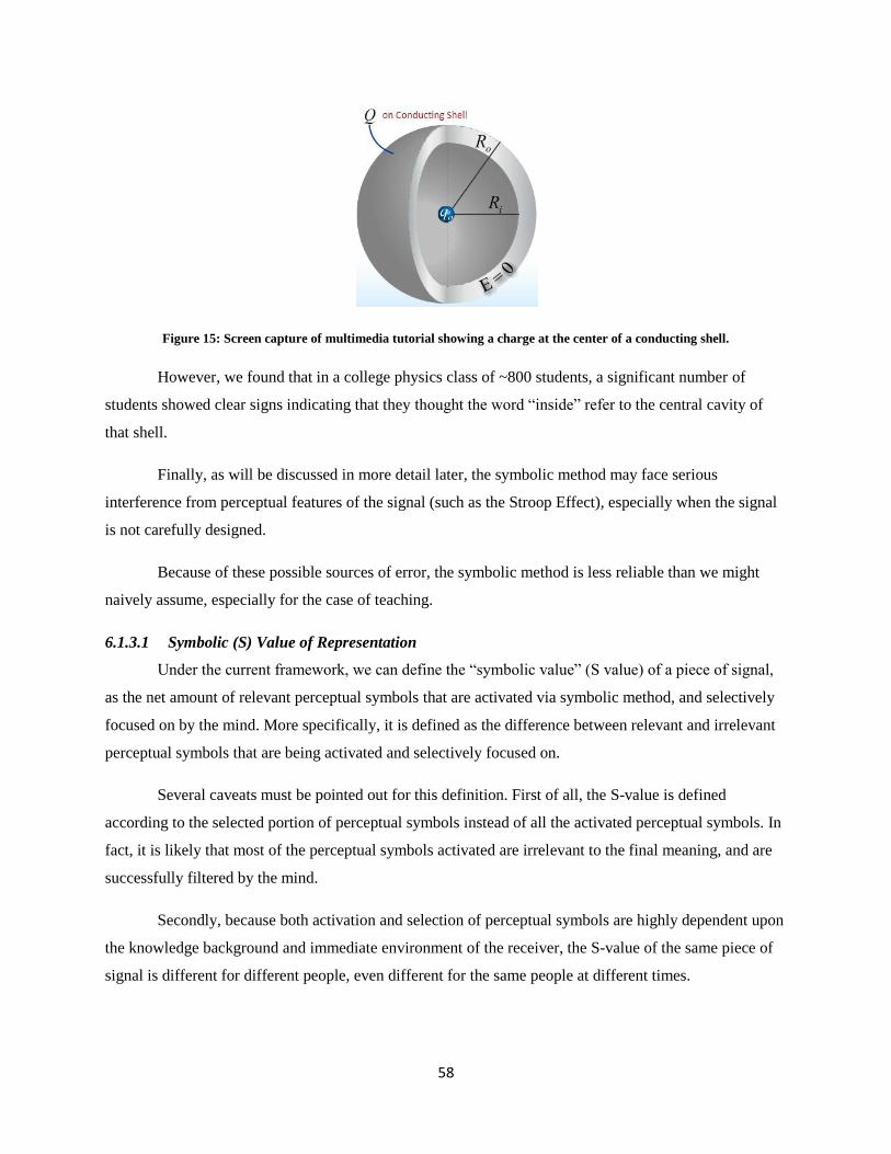
58
Figure 15: Screen capture of multimedia tutorial showing a charge at the center of a conducting shell.
However, we found that in a college physics class of ~800 students, a significant number of
students showed clear signs indicating that they thought the word “inside” refer to the central cavity of
that shell.
Finally, as will be discussed in more detail later, the symbolic method may face serious
interference from perceptual features of the signal (such as the Stroop Effect), especially when the signal
is not carefully designed.
Because of these possible sources of error, the symbolic method is less reliable than we might
naively assume, especially for the case of teaching.
6.1.3.1 Symbolic (S) Value of Representation
Under the current framework, we can define the “symbolic value” (S value) of a piece of signal,
as the net amount of relevant perceptual symbols that are activated via symbolic method, and selectively
focused on by the mind. More specifically, it is defined as the difference between relevant and irrelevant
perceptual symbols that are being activated and selectively focused on.
Several caveats must be pointed out for this definition. First of all, the S-value is defined
according to the selected portion of perceptual symbols instead of all the activated perceptual symbols. In
fact, it is likely that most of the perceptual symbols activated are irrelevant to the final meaning, and are
successfully filtered by the mind.
Secondly, because both activation and selection of perceptual symbols are highly dependent upon
the knowledge background and immediate environment of the receiver, the S-value of the same piece of
signal is different for different people, even different for the same people at different times.

59
Finally, since we cannot precisely measure the knowledge background and mental state of each
receiver, the S-value of a piece of signal cannot be precisely measured for any individual. However, it is
possible to roughly estimate the S-value of a piece of signal following two general principles. First of all,
the S-value of a signal is inversely proportional to the background different between the sender and the
receiver. Secondly, the more the sender understands the receiver’s background knowledge, the more
likely he is able to generate signal with higher S-value. This suggests that experts in general may not be
good teachers for introductory courses due to the large background difference, but they can improve their
teaching by gaining experience with students or learning about students’ difficulties from education
research.
6.1.4 The Perceptual inference (P) Method
When a piece of signal is perceived, neural circuits in the perceptual domain responsible for the
perception of the signal are activated. The perceptions made about the signal activate other tightly
associated perceptual symbols via perceptual inference. Both direct perception and inferred perceptual
symbols serve as potential resources for the brain to select and construct new simulations from. For the
sake of simplicity, we will refer to both as perceptual symbols, since direct perception functions almost
exactly the same as perceptual symbols when it comes to the construction of meaning (Figure 16).
Figure 16: The perceptual inference (p) method of resource activation (Continued from Figure 13).
As discussed above, any piece of signal that is selected by sensory memory, be it text, math symbol or
graph, will activate perceptual symbols through the perceptual method, regardless of whether such
activation was intended by the creator of the signal. For most signals, however, the majority of perceptual

60
symbols activated via the P-method are irrelevant to its intended meaning. For example, upon perceiving
the small blue sphere representing the positive charge in the previous example, the perception of its size,
color and shape of the sphere are all irrelevant to the understanding of the physics concept of the charge
and should be neglected.
If not actively suppressed by the brain, these irrelevant perceptual symbols would have a high
probability of interfering with relevant perceptual symbols activated and selected through the S-method,
by competing for the same neural circuits. As mentioned above, suppressing of these irrelevant perceptual
symbols places a small but detectable cognitive load on the brain, although in most cases such
suppressions are likely performed subconsciously.
Conventional physics representation design often includes many irrelevant perceptions. For
example, when we talk about how the voltage drop is divided across a large and a small capacitor in series,
the common practice (Figure 17) is to show two identical capacitors, indicate the voltage drop across
them, and write the mathematical expression next to the graph. A number of perceptions are in conflict
with its intended meaning in this representation. First of all, the perception of both capacitors being the
same size has to be filtered, since it activates the perceptual symbol of equivalence and uniformity among
the capacitors. Secondly, the voltage drops are represented by two similar letters with identical size,
which should be filtered for the same reason. Lastly, the letters may suggest voltage is a property that is
coagulated on the capacitors, and irrelevant to the wires connecting them, which is also irrelevant.
Figure 17: Conventional representation for capacitance circuit.
Unfortunately, these irrelevant perceptions are likely neglected by most instructors when creating
the representations, since their background knowledge allows them to easily identify and filter these
irrelevant perceptions, often without conscious attention.
However, we believe that for novices who are still learning the relevant background knowledge,
the cumulative cost of having to select and suppress large numbers of irrelevant perceptual symbols

61
coming from the p-method could be overwhelming, resulting in various forms of learning difficulties (the
specific forms of these learning difficulties will be listed later in this chapter). Sloutsky et. al. showed that
the amount of (irrelevant) visual features on symbols used in teaching abstract rules are inversely related
to the learning outcome (Sloutsky, Kaminski, & Heckler, 2005). We suggest that interference from
irrelevant perceptual features serves as a major cause of learning difficulties, yet unfortunately, has not
acquired much attention from researchers.
On the other hand, perceptual features of a piece of signal could be designed to reinforce, rather
than contradict, its intended meaning. For instance, in the previous example, the sizes of the capacitor
symbols could correspond to their relative magnitude. In that case, the interference between the P-method
and S-method would be constructive rather than destructive.
In addition to facilitating the understanding of S-method, the P-method also serves as an
independent method for activating perceptual symbols as resources. Compared to the S-method, which
suffers from miscommunication caused by inevitable expert-novice differences, the P-method is much
more reliable during teaching, since perception and perceptual inference are in general much less affected
by background knowledge. For instance, in the afore mentioned case of conducting shell, while saying the
word “inside” easily causes misunderstanding, simply highlighting the corresponding area would
certainly have avoided any potential misinterpretation. According to grounded cognition, P-method not
only conveys visual-spatial information, but can be used to facilitate any type of knowledge including
abstract concepts.
6.1.4.1 Perceptual (P) Value of Representation
Similar to the definition of the S-value, we can define the P-value of a representation as the
amount of net relevant perceptual symbols activated and selected via the P-method. Notice, however, that
although the filtered irrelevant perceptual symbols are not directly included in the definition, it has
significant indirect impact on the P-value. Most obviously, since the total number of perceptual features a
piece of signal possesses is constant, the presence of more irrelevant perceptual features means less
relevant perceptual features. More importantly, the more irrelevant perceptual features there are, the
greater the cognitive effort required to properly identify and filter them, and the more likely that the
process will be inaccurate. Therefore, the presence of a large number of irrelevant but relatively
insignificant perceptual features could be an indication that the P-value of a certain representation design
might be negative to students.
Like the S-value, the P-value is also dependent on the signal receiver, and also at the current stage can
only be roughly estimated for a given population of students. Despite this, the definition of P-value is still

62
a significant advance over the existing theories, since Mayer’s theory is unable to judge the effectiveness
of visual representation design on its own, and Schnotz’s criteria are only applicable to a very limited
number of cases.
6.1.5 The Categorical Inferences Method and the C Value of representation:
Once a new simulation is constructed out of the perceptual symbols activated via S and P
methods, the brain can then categorize this simulation, and draw categorical inferences from existing
categories. As explained in section 5.4, categorical inferences are themselves perceptual symbols, which
can be incorporated into the new simulation. This enriched new simulation, (or several simulations), is
then stored in long term memory, either as part of an existing concept, or as the first simulation of a new
concept. (Figure 18)

63
Figure 18: The Categorical inference (C) method. A): The initial simulation activates the category concept in LTM. B)
The concept creates a simulation (simulations) containing categorical inferences. C) Categorical inferences are added as
resources to enrich the current simulation, which is stored in LTM.
A
B
C

64
The perceptual symbols that are activated as categorical inferences via the C-method depend solely on the
quality of the initial simulation generated via the S and P methods. This means that the C-value of any
representation, defined as the net amount of relevant resources activated via the C-method during learning,
should be solely determined by its S and P values. In other words, the total value of any piece of
instructional material (to a particular student), should also be solely determined by its S and P values to
that student.
An implicit presumption behind this statement is that the ability to correctly categorize something into a
certain category is largely uniform amongst students. This assumption seems largely unproblematic when
we consider categories of higher hierarchy such as “object” and “process”, since these categories should
have been fully developed and extremely stable for any normal college student.
Associating the C-value of a piece of instructional material to its S and P values resolves the dilemma we
proposed earlier in section 2.3.1: why do students often end up with problematic categorization, even if
the instructor uses predominantly words from the correct category?
First of all, under PSS, categorization is performed based on perceptual symbols in a simulation, rather
than on words or semantic feature lists of a concept. Therefore, being exposed to a list of correct words is
no guarantee for correct categorization, unless these words can successfully activate the desired
perceptual symbols in the students’ mind (high S-value). Unfortunately, the S-value of verbal expression
is largely unrelated to its ‘technical correctness’. In other words, the same piece of text can easily be both
technically impeccable and practically confusing to a student at the same time.
In addition, the C-value of instructional material also depends on its P-value as well. Irrelevant perceptual
symbols activated via the P-method can seriously interfere with the interpretation of words. In physics
education, for example, the common visual representation of the electric field (Figure 19A) may interfere
with students’ understanding of “electric potential as the accumulation of electric field”, since it
perceptually looks like one single object, which conflicts with the simulation of the “accumulation”
process. In addition, the popular conventional representation of “Va-Vb”, consisting of only points and
letters (Figure 19B), provides no perceptual symbols relevant to the simulation of “accumulating electric
field from A to B along a certain path”. On the contrary, the blank area between the points perceptually
suggests that it is irrelevant, since irrelevant areas are always blank.
These conventional representation methods with low and probably negative P-value, while all being
technically unproblematic, make it difficult for students to simulate electric potential difference as the

65
result of an “accumulation process”. Rather, many students tend to think of it as a “local property” that
can be calculated from the local electric field at that point using kQ/R, just like the density of an object
can be calculated from its own weight and volume, and is independent of any change that happens to a
nearby object. On the contrary, the result of an “accumulation process” is affected by spatially distant
changes, such as the height at the tip of a pile of log will decrease if some pieces in the middle are taken
away.
As a result, students who categorizes electric potential as a ”local object”, will have much difficulty
understanding why the electric potential at one point will change when a neutral conducting shell is
placed a distance away from that point, which brings no change to the local electric field. (for example
see Figure 20)
Figure 19: Conventional physics representation that may interfere with proper categorization of electric potential. A)
Representation of electric field. B) Representation of potential difference.
In conclusion, we propose that the quality of instructional materials should be determined by the number
of relevant perceptual symbols it can activate in the students’ mind, rather than the number of words or
figures that can be determined as “correct” by any expert.
6.2 The impact of instructional material design on problem solving
Instructional material with adequate S and P values allow the learner to generate and store correct
simulations. On the other hand, those with low S or P values will either lead the learner to generate and
store an incorrect simulation, or confuse the learner so much that he is unable to create any coherent
simulation at all.
The previously mentioned case of “electric field inside a conducting shell” serves as a good example of
“incorrect simulation”: a simulation that is very different from what was intended by the instructor.
A B

66
Incorrect simulations may often end up belonging to a different ontology. For example, it is well
documented that students often simulate electric current as charges coming out of the positive plate of the
battery and reaching the negative plate after spending some time traveling through the circuits. According
to Chi, such a simulation belongs to the “object” ontology, while the correct simulation of the current
should belong to the “process” ontology.
Instructions with negative S and P values activate a large amount of irrelevant perceptual symbols in the
learner’s mind. When too many irrelevant perceptual symbols are present, the learner looses the ability to
identify and select a coherent subset to construct a simulation from. In other words, the material simply
doesn’t make much sense to the learner.
Normally, people would try to resolve the inconsistency in their understanding, either by thinking harder
or asking for help. However, we suspect that when students are subjected to the pressure of learning the
content in a given amount of time, or when adequate help is not immediately available, they would turn to
rote learning or shallow learning as an alternative strategy.
In the framework of the current model, we can define rote learning as storing the holistic direct perception
of the signal itself in long term memory, in place of the intended simulation. Technically speaking, these
perceptions are also stored as a simulation, except that the perceptual symbols contained in this simulation
are very different from the ones intended by the instructor. More precisely, rote learning often results in a
simulation that contains an excessive amount of unnecessary direct perception, and little inferred
perceptual symbols corresponding to shallow understanding of the meaning.
According to our current model, rote learning might be a natural response to confusing
instructions. When a lot of perceptual symbols activated through S and P methods are in contradiction
with each other, or contradicts common sense, their strength of activation is likely to be weaker. The most
significant signal left in the sensory/motor domains, in that case, would be the perception of instruction
itself. Consequently, they have a high chance of being recorded in LTM.
Naturally, both incorrect simulation and rote learning lead to various difficulties in problem
solving. We here propose that several types of difficulties that are frequently observed among novice
physics students can be directly linked to either incorrect simulation or rote learning.
6.2.1 Problem Solving
When facing a physics problem, the solver thinks about relevant physics concepts according to the
problem context. In grounded cognition terms, to “think about” a concept means that the brain generates a
simulation from that concept, which is coherent with the problem context. Although the generated

67
simulation is not exactly the same as any previously stored simulation, it is almost certainly based upon
one or more of them. However, exactly which previous simulation(s) will the new simulation be based
upon depends on various factors, including problem context, solver’s cognitive and bodily state, as well
as background simulation (See Chapter 4).
6.2.2 Incorrect simulation
When the new simulation is based upon an incorrect previous simulation, or one that doesn’t suit the
current problem, then the solver will end up with a wrong answer. As was discussed in section 2.3, in
many cases the new simulation will be unproductive if it happens to belong to a wrong ontological
category, or more precisely speaking, an ontological category that is different from the one that should be
used for the current problem.
Hammer’s dynamic ontology view suggests that a student is able to shift between different ontologies
under proper guidance. This scenario corresponds to the case that multiple simulations of different
ontology are stored under the same concept. Therefore, by changing external conditions, a different
previous simulation can be activated to create a different new simulation, which may be productive in the
current case.
However, for students studying some of the more difficult physics concepts, it is possible that a majority
of the previously stored simulations belongs to a single ontological category (often unproductive), due to
constant exposure to low quality instructional materials. For example, many students can only simulate
electric potential as created by a local electric field. In that case, generating a simulation with a different
ontology is virtually impossible for these students regardless of the external conditions. As a result, they
will display “ontology stubbornness” similar to that observed by Chi et. al. (Slotta et al., 1995)
From a grounded cognition perspective, to help students overcome ontology difficulty is to enable the
concept to generate a new type of simulation. The most direct method is to provide the essential
perceptual symbols necessary for the new simulation via instructional materials with high S and P value.
For example, in the first experiment, if a student is unable to simulate electric potential as the
accumulation of electric field, then the most effective way is to directly show him the accumulation
process, or technically speaking, provide him with essential perceptual symbols for creating the
accumulation simulation via both S and P method, especially the P method.
6.2.3 Rote Learning
Rote learning, on the other hand, results in some different types of difficulty in problem solving. Rote
learning stores holistic direct perception of the instructional material itself, instead of a proper simulation

68
generated from that. The first problem it creates is that the concept can only be activated, and will be
easily activated, by problem context of high surface similarity with the remembered instruction, such as
sentences containing the same words or similar pictures.
For example, if a student learns entirely by rote that “charges on a metal bar traveling in magnetic field
will move due to the Lorentz force”, then this piece of knowledge can only be activated via problems of
high surface similarity such as “what do electrons in a metal bar do when traveling in magnetic field”. It
is almost impossible for him to even think about that knowledge when facing the problem “why will there
be a slight potential difference between the two tips of the wings of a plane when flying in the earth’s
magnetic field?”. Yet, it is highly likely that when given the problem “what will happen to charges on an
insulating bar if it is traveling in a magnetic field”, he will answer “charges will move” simply because
the words are similar.
One needs to look no further than the autobiography of Richard Feyman to find perfect real life examples
of rote learning, which occurred in the chapter describing his teaching in Brazil (Feynman, 1985).
On the other hand, a correct simulation consists mostly of perceptual symbols inferred from S, P and C
methods from the instruction, and only a small fraction of direct perception from the signal itself. For a
relevant problem, although the problem body may present very little surface similarity with the original
instruction, the problem context will activate much of the same perceptual symbols contained in the
simulation. (The simulation of an airplane has much in common with the simulation of a metal bar)
Therefore, the problem has a good chance of activating the correct knowledge. For an irrelevant but
superficially similar problem, although it has much surface similarity with the instruction, most of the
surface features of the instruction itself has been discarded during learning. Therefore the problem only
has a small chance of activating the knowledge.
Notably, the idea of activating appropriate knowledge via inferred perceptual symbols is very similar to
the notion of “secondary inference” suggested by Chi et. al. in her well known study of problem
categorization (M. Chi & Feltovich, 1981).
Verbal rules that are learned by rote might have an exceptionally high chance of being (improperly)
activated. Barsalou and others have proposed that there is a “word processing” system in the brain, which
performs superficial reasoning based purely on statistical frequency of word association(Lawrence W.
Barsalou et al., 2008). Upon receiving verbal signal, that system is activated slightly earlier than the more
fundamental simulation system which carried out actual thinking. Therefore, rote learned knowledge
might reduce the chance of simulations stored in the same concept for being activated.

69
Furthermore, rote learning likely impairs students’ ability to construct and implement a multi-step
solution. Planning a multi-step solution requires the solver to generate and hold multiple simulations in
mind, which is very cognitively demanding. Rote learning causes a concept to regenerate the direct
perception of a piece of signal, which cannot be directly processed by the simulation system of the brain.
In order to continue further reasoning, one must first translate that piece of signal into a simulation (think
about what the sentence means in this problem). This extra task likely leaves the brain with insufficient
cognitive capacity to generate and hold enough simulations to solve the problem. For a problem that
requires a multi-step solution, this means that rote-learning students are less likely to identify whether an
intermediate step can eventually lead to the final answer, and have a higher tendency to generate a one-
step superficial answer.
6.2.4 No simulation.
In addition to the above mentioned cases, it is also likely that the students’ concept lacks the
ability to generate any meaningful simulation that is coherent with the problem context. In that case,
students may be forced to turn to alternative strategies of problem solving, such as blind equation hunting
or mathematical manipulation, since these strategies do not require much understanding of the physics
behind the problem to implement.
While all the aforementioned student behaviors have long been documented and widely studied,
previous researchers have either attributed their origins to the interference of naïve misconceptions from
everyday life (section 2.1), or to epistemological/psychological reasons (Elby, 1999), or implicitly treated
them as inevitable barriers during learning, which requires additional activities to overcome (see for
example McDermott & Shaffer, 1992). Our model is the first to explicitly link these behaviors to
discrepancies in the design of instructional materials. We predict that all of these problems can be reduced,
and even disappear, simply by improving the instructions for content knowledge, which improves the
students’ ability to generate proper simulations from physics concepts.

70
7 Experiment 1
7.1 Multimedia Design and Predictions
In experiment 1, we intend to verify the hypothesis that ill-designed representations could be at least
partly responsible for conceptual difficulties among students. Furthermore, we will test whether the
multimedia learning model constructed in the previous section has the power to identify flaws in the
design of instructional material, and provide guidance to improving its quality.
According to the current model, designing flaws in instructional materials could result in either low S
value or low P value. However, in most cases, flaws resulting in low S values are easier to identify, such
as containing words or expressions that are unfamiliar to the students, or containing a graph with no
legends. Careful and experienced instructors can usually avoid those mistakes with relatively little
difficulty.
Flaws that result in a low P-value, on the other hand, are much less obvious to most instructors,
since they possess ample background knowledge to filter out irrelevant perceptions. Many conventional
physics representations that have been used for decades probably have negative P-values for most
students, a typical example being the diagram for electromagnetic waves (Podolefsky & Finkelstein,
2007). Moreover, some of us may think of representations such as circuit diagrams as being
predominantly symbolic, and therefore perceptual features of these symbolic diagrams should be
irrelevant to understanding, in much the same way as the size of math symbols are thought of as irrelevant
to judging their value. Therefore perceptual imperfections are frequently being neglected by instructors.
Furthermore, traditional static visual representations face many physical restrictions from the media,
preventing them from providing many visual features such as continuous motion, resulting in a low P-
value.
Because of that, we will focus on low P-value instructions in the both experiments. According to
our model, the perceptual features of representations could have a direct impact on the final knowledge
constructed from them by the learner. In other words, our model predicts that students who received low
P-value instructions are more likely to display behaviors as a result of failed learning, such as ontological
stubbornness, rote or shallow learning, and equation hunting. On the other hand, if the P-value of the
same piece of instruction is increased by redesigning its visual representation, even if the amount of
“information” conveyed by the tutorial stays unchanged, we would still expect to see students
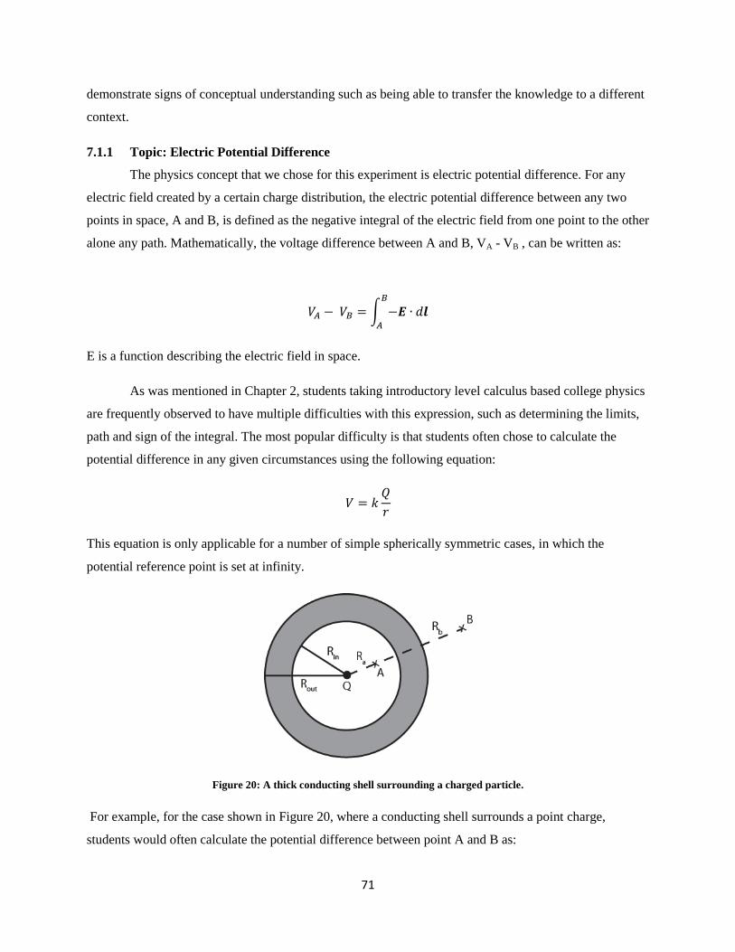
71
demonstrate signs of conceptual understanding such as being able to transfer the knowledge to a different
context.
7.1.1 Topic: Electric Potential Difference
The physics concept that we chose for this experiment is electric potential difference. For any
electric field created by a certain charge distribution, the electric potential difference between any two
points in space, A and B, is defined as the negative integral of the electric field from one point to the other
alone any path. Mathematically, the voltage difference between A and B, VA - VB , can be written as:
∫
E is a function describing the electric field in space.
As was mentioned in Chapter 2, students taking introductory level calculus based college physics
are frequently observed to have multiple difficulties with this expression, such as determining the limits,
path and sign of the integral. The most popular difficulty is that students often chose to calculate the
potential difference in any given circumstances using the following equation:
This equation is only applicable for a number of simple spherically symmetric cases, in which the
potential reference point is set at infinity.
Figure 20: A thick conducting shell surrounding a charged particle.
For example, for the case shown in Figure 20, where a conducting shell surrounds a point charge,
students would often calculate the potential difference between point A and B as:

72
Several possible causes of this difficulty have been mentioned in previous chapters. In particular,
the most probable cause seems to be that students treat electric potential as a local property that is created
by the local electric field at that point:
, in much the same way as the mass of an object results in its
weight. Therefore, comparing the potential difference between two points is like comparing the weight
difference of two objects, which should not depend on anything in between the two objects. The idea that
potential difference is defined by accumulation of the electric field along a line is hard to get across to
students.
We believe that this difficulty at least partly originates from the fact that conventional visual
representations used in the teaching of electric potential have low P-values for students at this level. We
will now examine the conventional representation, and show that it does contain a large number of
irrelevant and conflicting perceptions. Since we are mainly interested in the idea of integral and
accumulation, we will restrict our discussion only to cases with spherical symmetry, for the purpose of
eliminating unwanted complexity in the discussion and in our experiment.
7.1.2 Conflicting Design in Conventional Representation
Several perceptual features in the conventional representation are in conflict with the
“accumulation” idea. First of all, the field line representation of the electric field, shown in Figure 21,
depicts the electric field as a holistic, continuous substance that extends throughout the entire space.
According to PSS, in order to activate the concept of “accumulation”, we must simulate the process of
“accumulation” (adding up smaller units to result in a big difference) at least partially and subconsciously.
However, the continuous and holistic electric field line representation does not seem to consist of
separable smaller fragments that could fit into the “accumulation” simulation. Therefore, the perception
of this field line representation needs to be suppressed and filtered, whereas the simulation of
“accumulation” needs to be constructed from ground zero. In this case, the P-value of the E-field
representation is negative for students with no background knowledge for electric field.

73
Figure 21: Conventional representation of the electric field around a charged particle
When illustrating the potential difference between two points, the conventional visual representation is
simply two dots labeled with VA and VB (Figure 22 A). When the definition of electric potential is
introduced as the integral of electric field along a path, a line with an arrow is then drawn from one point
to another9 (Figure 22 B). More careful instructors would emphasis that dl stands for a small segment on
which the electric field is treated as constant, and the integral means dividing the path from A to B into
infinitely many small pieces of dl, and adding up the electric field for each small segment of dl. In that
case, the visual representation may be an arrow going through multiple points along the path. (Figure 22
B)
Figure 22: Conventional representation of electric potential differencde and integral of electric field. A) Electric potential
difference is represented by similar looking text lables. B) The integral porcess is represented as an arrow passing
through multiple segments representing dl.
In these designs, several perceptual features are in conflict with the concept of “difference caused
by accumulation”. First of all, the “difference” in potential between the two points is not perceived. The
two labels are almost identical, and the two points are identical, therefore, the brain has to filter the
perception of the “sameness”, and generate a simulation of “difference”. More importantly, the process of
“accumulation” is represented with an arrow moving through space. Perceptually, the arrow has uniform
width and color, and contains no perception that could be related to the concept of “accumulation”. In
addition, the subject that is being accumulated over distance: the electric field, is not perceivable.
9 To eliminate unwanted complexity, we will restrict our discussion to the case in which the two points are placed
along the radial direction, which means that the optimal path for the integral is a straight line between the two surfaces.
74
“Accumulation leading to difference” is a very natural idea, quite possibly a p-prim that could
come from numerous real life experiences of collecting things. However, since in this conventional
representation, none of the perceptual features are related to either “accumulation” or difference. Students
perceive two apparently unrelated entities, an arrow and two labels, and are told that one leads to another.
Since visual representation interferes with interpretation of verbal explanation, students will be driven to
learning the explanation by rote. In other words, the P-value of this representation is likely very negative.
Notice that none of the multimedia learning theories reviewed in chapter 0 could confidently
predict that this representation will have a negative effect on learning. According to Mayer’s theory,
multimedia learning material supports learning when verbal information are simultaneously accompanied
by corresponding visual representation. Judging from this criteria, the aforementioned representation
contains visual representations for all the objects mentioned in the verbal explanation of electric potential,
from “electric field”, “potential” to “integrate”. Therefore, as long as the verbal and visual materials are
delivered simultaneously, the instruction should facilitate understanding as the brain should be able to
actively make “links” between visual and verbal representations that result in better understanding.
On the other hand, Schnotz argues that visual representation should be suitable for the given task.
Therefore, as long as we ask questions regarding similar spatial constructs, then this representation should
be the most suitable choice.
On the contrary, our grounded cognition model not only suggests that the conventional
representation is problematic, but also points to detailed aspects for improvement. We here introduce our
own design of a new visual representation aimed at improving the P-value of the representation.
7.1.3 Perceptually enhanced design
We have just pointed out three different aspects of the conventional physics representation that
contains conflicting perceptions: the holistic electric field, the potential difference, and the accumulation
process. We will first redesign the visual representation of potential difference. The guideline for creating
such a representation is simple: a good representation of potential difference should visually look very
different at points A and B. This is because according to grounded cognition principles, at least part of the
neural circuits that creates a simulation representing the idea of “difference”, should also be in charge of
identifying a difference visual perception. Therefore, the perception of difference should facilitate the
understanding of the corresponding concept.
Among a number of possible visual designs, we chose to represent potential difference with the
color and thickness of equipotential surfaces, as shown in Figure 23 and Figure 24. The benefit of this

75
design is that it is relatively easier to detect small thickness changes on a ring, compared to smaller shapes
such as a dot. Therefore, we can demonstrate gradual change of thickness over a wider range without the
rings overlapping each other. We use both the line thickness and color saturation to create a strong visual
perception of difference between lines when showing the accumulation process.
It should be pointed out that the direct perception of color and line thickness are both irrelevant to
the electric potential. However, it could be safely assumed that a university student, even with little
knowledge of electric potential, should know very well that electric potential probably has neither color
nor shape, and should filter out these perceptions with little difficulty. The relative magnitude of electric
potential is conveyed through perceptual inference.
Since we have used equipotential surfaces to represent potential differences, the local electric
field could naturally be represented by radiating arrows in between. The density and saturation of the
arrows roughly corresponds to the magnitude of the electric field between the lines. This piece-wise
representation of electric field seems much more perceptually compatible with the idea of “accumulation”.
Figure 23: Perceptually enhanced representation of potential difference and electric field. Potential difference is
represented as colored equipotential surfaces with different colors(see also Figure 24). Electric field is represented by
black arrows in between
The visual effect of “accumulation” is created through animation, in which equipotential lines
appear one after another from one point to another. Before each new equipotential line appears, the local
electric field appears briefly, and a new ring emerges from the previous one, and moves across the electric
field while its thickness and color changes gradually.
Line thickness, color saturation (the amount of white in the color), as well as a color gradient
from blue to red, combine together to provide a strong visual perception of electric potential changing
from weak to strong. The change of all three factors roughly resembles the actual change of electric
potential in space.
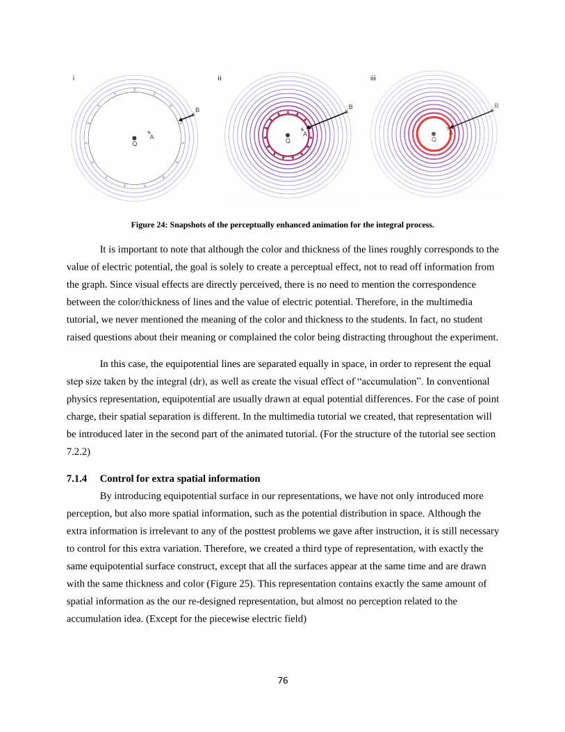
76
Figure 24: Snapshots of the perceptually enhanced animation for the integral process.
It is important to note that although the color and thickness of the lines roughly corresponds to the
value of electric potential, the goal is solely to create a perceptual effect, not to read off information from
the graph. Since visual effects are directly perceived, there is no need to mention the correspondence
between the color/thickness of lines and the value of electric potential. Therefore, in the multimedia
tutorial, we never mentioned the meaning of the color and thickness to the students. In fact, no student
raised questions about their meaning or complained the color being distracting throughout the experiment.
In this case, the equipotential lines are separated equally in space, in order to represent the equal
step size taken by the integral (dr), as well as create the visual effect of “accumulation”. In conventional
physics representation, equipotential are usually drawn at equal potential differences. For the case of point
charge, their spatial separation is different. In the multimedia tutorial we created, that representation will
be introduced later in the second part of the animated tutorial. (For the structure of the tutorial see section
7.2.2)
7.1.4 Control for extra spatial information
By introducing equipotential surface in our representations, we have not only introduced more
perception, but also more spatial information, such as the potential distribution in space. Although the
extra information is irrelevant to any of the posttest problems we gave after instruction, it is still necessary
to control for this extra variation. Therefore, we created a third type of representation, with exactly the
same equipotential surface construct, except that all the surfaces appear at the same time and are drawn
with the same thickness and color (Figure 25). This representation contains exactly the same amount of
spatial information as the our re-designed representation, but almost no perception related to the
accumulation idea. (Except for the piecewise electric field)

77
Figure 25: Representation of electric potential designed as a control for the extra spatial information.
7.1.5 Current Multimedia Learning Theories on These Three Representations:
Current multimedia learning theories have very limited power at distinguishing between these
three representations.
In Mayer’s multimedia principles, the one principle regarding the quality of visual representation
design is that interesting but irrelevant materials should be avoided. However, Mayer does not provide a
clear criteria for judging the relevance of visual perceptions. Therefore, from an amodal symbol point of
view, one could argue that since electric potential has neither color nor shape, and math expressions are
purely symbolic arguments, the colored lines and flashing arrows serve as significant distraction. In fact,
when the perceptually enhanced representation is played on a computer, the screen does seem extremely
busy.
If that argument is valid, then the learning outcome would be best for the conventional design,
and worst for the perceptually enhanced design, with the control of information design somewhere in
between.
Schnotz’s theory argues that visual representation should be compatible for the given task. Again,
in this case the difference between the visual representations is so small that judging task compatibility
becomes difficult. One might argue that for spherically symmetric geometry, spherical equipotential
surface is a more task suitable representation. In that case the control of information design should be as
effective as the perceptually enhanced design. However, since the symmetry of the electric potential
distribution is irrelevant to any of the posttest problems, the differences should be very small, if any.
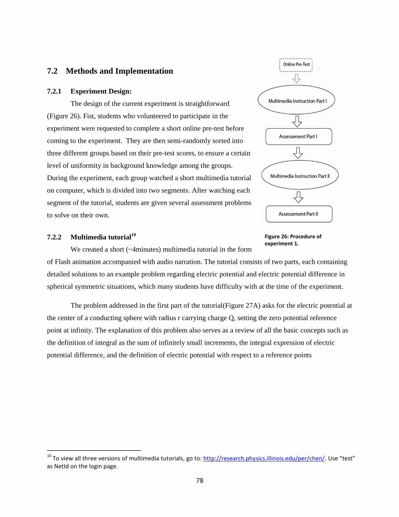
78
7.2 Methods and Implementation
7.2.1 Experiment Design:
The design of the current experiment is straightforward
(Figure 26). Fist, students who volunteered to participate in the
experiment were requested to complete a short online pre-test before
coming to the experiment. They are then semi-randomly sorted into
three different groups based on their pre-test scores, to ensure a certain
level of uniformity in background knowledge among the groups.
During the experiment, each group watched a short multimedia tutorial
on computer, which is divided into two segments. After watching each
segment of the tutorial, students are given several assessment problems
to solve on their own.
7.2.2 Multimedia tutorial10
We created a short (~4minutes) multimedia tutorial in the form
of Flash animation accompanied with audio narration. The tutorial consists of two parts, each containing
detailed solutions to an example problem regarding electric potential and electric potential difference in
spherical symmetric situations, which many students have difficulty with at the time of the experiment.
The problem addressed in the first part of the tutorial(Figure 27A) asks for the electric potential at
the center of a conducting sphere with radius r carrying charge Q, setting the zero potential reference
point at infinity. The explanation of this problem also serves as a review of all the basic concepts such as
the definition of integral as the sum of infinitely small increments, the integral expression of electric
potential difference, and the definition of electric potential with respect to a reference points
10
To view all three versions of multimedia tutorials, go to: http://research.physics.illinois.edu/per/chen/. Use “test” as NetId on the login page.
Figure 26: Procedure of experiment 1.

79
.
Figure 27: Illustration of the two problems used in the multimeida tutorial. A) Find the potential V(0) at the center of a
neutral conducting shell. The zero potential reference point is set at infinity. B) A positive charge Q is enclosed in a
conducting shell. What will happen to the potential difference between points A and B if the shell is enlarged?
In the example used in the second part of the tutorial (Figure 27B), a point charge with charge Q
is enclosed at the center of a thick neutral conducting shell. Two points, A and B, are separated by the
shell. The problem first asks for the potential difference between points A and B, then asks what would
happen to the potential difference, if the radius of the shell is increased while keeping the thickness
unchanged (Assuming that A and B are still separated by the shell.) This problem, together with its
solution, serves to address an important yet very obvious categorical inference of the category
“accumulated value”: the total accumulated value (potential difference) is larger if a smaller part of
what’s being accumulated (electric field) is taken away.
Also, the more common way of drawing equipotential surfaced at equal potential difference is
introduced in this part. (see section 7.1.3)
Three different versions of the multimedia tutorial were created, each using one of the three
different designs explained in the previous section. However, only two slightly different versions of
accompanying audio narration are created, one for the traditional representation version, and one for both
the enhanced perception version and the information control version. The two versions of audio narrations
are only different in the following two aspects: 1. The word “points” in the traditional version is replaced
by “equipotential surfaces” in the other version. For example, the sentence “voltage difference between
the two points” in the first version is replaced by “voltage difference between the two equipotential
surfaces” in the second version. 2. A short extra paragraph is added in the second version at the beginning
of the tutorial, with the sole purpose of introducing equipotential surfaces.
The audio script for the traditional version was first created, and later modified into the second
version, to ensure that the wording of the solution is not biased towards an equipotential representation.
Nowhere in the script did we mention the meaning of visual elements such as color and thickness of the

80
equipotential rings. Both audio scripts were created and examined by experienced instructors to ensure
their quality. Both audio scripts were read and recorded by the same instructor, with very similar speed,
tone and voice.
A flash animation is first created for the enhanced perception version, due to its technical and
graphical complexity. The animation is later modified into the other two versions by replacing or
removing certain visual elements, to ensure that the three animations are identically synchronized with the
audio scripts. All three versions were inspected by experienced instructors of the electricity and
magentism course to ensure that no misunderstanding would arise as a result of apparent discrepancy in
animation design.
The tutorial is designed for students who have some basic knowledge of electric field and Gauss’ law, are
familiar with properties of conductor and insulators, and have been introduced to the nomenclatures
related to electric potential, yet still have much difficulty with solving both problems in the tutorial.
The tutorial is designed for experimental purposes, instead of instructional ones. Therefore, it only covers
the special case of positive charge(s) in spherical symmetry, and neglects the details such as selecting the
proper path of integral, determining the sign of the integral, and non-spherical symmetric cases.
7.2.3 Assessment
The assessment used in this experiment consists of 14 problems; some of the problems have
multiple questions (see appendix) and are divided into two parts. Some of the problems are asked to
assess the knowledge we intend to teach, while the other problems serve to remind students of related
knowledge that is not covered in the tutorial, but required to solve the problem, such as how to calculate
the electric field in space. These electric field problems are very easy for average students in the class.
Students are asked to provide explanations to most multiple choice question, except for PI-4 and PII-1 for
obvious reasons.
The last problem in part I of the tutorial, PI-8, is the same as the example problem used in the second part
of the tutorial.
Part I of the assessment is given to students after they have completed the first part of the tutorial,
but not the second part. Part II of the assessment is given to students after they have completed both parts
of the tutorial. Students are instructed not to go back and change their answers in Part I once they’ve
proceeded to watching tutorial part 2.
81
At the end of the assessment, students are asked to rate the quality of the animated tutorial on a scale of 1-
10.
7.2.4 Participants and the timing of participation
We recruited a total of 61 undergraduate students from the fall 2010 class of the calculus based
electricity and magnetism course to participate in the experiment. The experiment is conducted near the
end of the semester, a couple of days before the final exam. We chose this time of the semester to
administer the experiment because of the following reasons. First, at this time students are more
motivated to learn the material as it will be tested on the final exam. Second, electric potential was being
taught near the beginning of the semester, and most students’ memory of this content is rather vague at
this point. This would result in better uniformity among students, since they are less likely to be
influenced by the memory of one or two particular problem(s) that they may have encountered before.
Students received $10 as a reward for participating in the experiment, which typically took
around 1 hour to finish.
7.2.5 Procedural details
The animations are distributed to students via Smartphysics™ multimedia player11
. The same
player is used weekly to distribute course materials for the electricity and magnetism course they are
taking, and therefore students are very familiar with the operation of the player.
Students are allowed to freely pause and rewind at any point of the multimedia tutorial. The
player sends the timestamp of each action (play, pause, rewind, stop) to a database on a remote server.
At the end of the first part of the tutorial, the player stops and advises students to complete the
first part of the assessment before continuing to the second part. Most (all but 2) of the students followed
the advice, according to the action data stored.
7.3 Experiment 1 Results
7.3.1 Participants and Background
A total of 61 students showed up for the experiment, 22 in group Ctrl. (conventional representaion), 21 in
group Exp (perceptually enhanced representation) and 18 in CInf (representation to control for extra
information).
A few students (<5 in each group) scored >=2 out of 3 points on the pretest. To ensure that students’
understanding of electric potential before the intervention was relatively weak and uniform among the
11
http://www.smartphysics.com/promo/

82
three groups, those who had scored 2 or more points out of 3 points on the pretest were excluded from the
final analysis (see Appendix I for pretest problems). The remaining population is 18, 20 and 16 for groups
Ctrl, Exp and Cinf respectively.
The average Hex 1 score for the remaining population is not significantly different between the three
groups, with the Ctrl group slightly lower and Cinf group slightly higher (p=0.2), as shown in the table
below. Hex 1 score is chosen as an indicator for students’ background content knowledge, since all of the
knowledge relevant to the problems in the posttest were learned before HEX1 and covered in HEX 1.
Ctrl Exp Cinf
HEX 1 65.77 ± 1.95 68.15 ± 1.88 71.19 ± 1.92
Table 3: Average scores on Hex 1 for each group.
7.3.2 Grading Scheme
Students’ answers for each question on both parts of the post test are first graded on a scale of 0-3. The
gradings for each problem is based on students’ written work and explanation of their reasoning (if
applicable), following the grading scheme listed in the table below.
Score Criteria
0 Completely wrong or no answer at all.
1 Showed some signs of understanding but made major mistakes.
2 Incomplete reasoning or minor mistakes.
3 Compeletely correct.
Table 4: Grading scheme for experiment 1 posttest problems.
Two individual graders graded all the students’ answers independantly at first. They then discussed the
grading with each other, and were able to reach consensus on the scores assigned to each each problem to
within 1 point. We will report analysis results based on gradings from both graders. Since no analysis we
performed showed major differences depending on the grader, we will only show graphs based on the
grading of Grader 1. (The graphs from Grader 2 were very similar).

83
Six questions relevant to electric potential were asked on posttest Part I, in which PI-6 and PI-7 are highly
correlated and graded as one problem. Therefore, the total points available for Part I of the posttest is 15.
Four questions on electric potential are given on Posttest part II (12 points in total).
7.3.3 Posttest Performance
The average posttest score, reported as the percentage of total points earned, is listed in Table 5 and
plotted in Figure 28.
As can be seen from the data, the average total score for the first part of the posttest slightly favors the
Exp group, while the average score for the second part of the posttest is significantly different between
the three groups, with Exp group having a higher average than both control groups. When comparing
between each two groups, simple t-tests on the posttest part II score yields p= 0.002 between Ctrl and Exp
group, and p=0.01 between Exp and Cinf group.12
(Scores are reported as the percentage of total possible
points for voltage problems in each part.)
Figure 28: Average posttest score for both part of the posttest. Posttest scores are reported as the percentage of total
available points earned.
12
Reported values are based on grading of grader 1. Same analysis on grading of grader 2 results in p = 0.0003 and p= 0.04 respectively.
0%
20%
40%
60%
80%
Part I Part II
% o
f p
oss
ible
po
ints
Ctrl
Exp
Cinf

84
Part I Ctrl Exp CInf P (ANOVA) θ Ctrl,Exp θ Exp,Cinf
Grader 1 29.26 ± 5.98% 46.33 ± 5.95% 35.83 ± 6.26% 0.13 0.64σ 0.24σ
Grader 2 31.48 ± 5.87% 46.67 ± 5.69% 39.58 ± 6.03% 0.19 0.59σ 0.27σ
Part II Ctrl Exp CInf P (ANOVA) θ Ctrl,Exp θ Exp,Cinf
Grader 1 42.59 ± 4.09% 67.08 ± 5.25% 46.88 ± 6.93% 0.004 1.17σ 0.79σ
Grader 2 40.27 ± 3.11% 65.00 ± 5.49% 51.04 ± 5.69% 0.002 1.24σ 0.59σ
Table 5: Students’ total score on both parts of the posttest. Scores are reported as percentage of points available in each
part. The θ column reports the effect size between two groups, σ stands for the pooled standard deviation between the two
groups.
To further investigate students’ posttest performance, we plotted the percentage of completely correct
answers (score = 3) in each group for every question on the posttest, as shown in Figure 29.
For every problem, the two graders are different by no more than 2 students within each group, and the
differences do not qualitatively change the results. (Grading of each grader on every electric potential
problem can be found in the Appendex (see the end).)
Figure 29: Correct rate for each electric potential problem. A) Correct rate for problems in Part I of the posttest B)
Correct rate for problems in Part II of the posttest.
As can be seen from the data, the Exp group outperformed both control groups on all problems.
0%
10%
20%
30%
40%
50%
60%
70%
80%
90%
100%
PI-1 PI-3 PI-4 PI-6&7 PI-8
% o
f co
rrec
t an
swe
r
Post test Part I
Ctrl
Exp
CInf
0
0.1
0.2
0.3
0.4
0.5
0.6
0.7
0.8
0.9
1
PII-1 PII-2 PII-4 PII-6
% o
f co
rrec
t an
swe
r
Post test Part II
Ctrl
Exp
Cinf
A
B
A B

85
Among the problems in part I, the Exp group significantly outperformed both control groups on P1-1. (p=
0.06 from grader 1, p = 0.02 from grader 2) P1-3 showed a similar but less significant trend (p = 0.25
grader 1, p = 0.14 grader 2) .
On part II of the posttest, the Exp group performed drastically better than both control groups on PII-1
and PII-6. (p<0.01 from both graders). Interestingly, PII-2 and PII-3 have a higher correct rate, and didn’t
shown much difference between the three groups.
7.3.4 Impact from students’ general ability
Given that students’ content knowledge on the subject is largely equivalent between the groups, the
difference on the posttest is likely caused by the difference in the multimedia tutorial. However, since our
sample size is rather small, it is also possible that other factors that are independent of students’ content
knowlege are non-uniform between the groups. These factors may also contribute to the observed
performance differences.
To measure how much these content independent factors such as math ability and learning habits are
different between the three groups, we look into their scores on other exams in the course: HEX2, HEX3,
and the final exam. Most of the content covered by those exams are not directly related to electric
potential, and therefore serve as indicators of students’ general ability. (
Table 6)
Another reason to look at these scores is because the experiment is carried out towards the end of the
semester, two months after HEX1. Students’ ability and understanding of E&M knowledge in general
might have changed during this period.
As can be seen in
Table 6, the exam scores of Exp group and Cinf group are almost identical, so that the differences on the
posttest cannot be attributed to difference in ability. However, students from the Ctrl group have lower
average HEX2, HEX3 and Final scores than the other two groups.
212 final hex1 hex2 hex3
Ctrl 65.16 ± 2.18 % 65.77 ± 1.95 % 63.22 ± 2.76 % 67.83 ± 2.69 %
Exp 73.40 ± 2.59 % 68.15 ± 1.88 % 74.70 ± 3.34 % 74.90 ± 3.17 %
Cinf 71.69 ± 3.13 % 71.19 ± 1.92 % 73.75 ± 4.06 % 74.13 ± 2.81 %
Table 6: Average exam scores of each group.

86
In order to understand how much (if at all) students’ exam scores correlate with their performance on the
posttest, we created scatter plots of posttest score vs. total exam score (Figure 30), which is defined as
(hex1+hex2+hex3 + 2*final)/5. The extra weight on final is because it is twice as long as the hour exams.
It is easy to see from these scatter plots that the correlation between total exam score and either part of the
posttest performance is fairly weak for all three groups. In fact, by performing a linear regression analysis
on each set of data, we found that the correlation coefficients (R2) in all cases are not significantly
different from zero, except for Cinf group in Part II.
Part I R2 p(t-test) α
Ctrl 0.003 0.83 0.2
Exp 0.082 0.22 0.8
Cinf 0.16 0.13 0.9
Part II R2 p(t-test) α
Ctrl 0.009 0.71 -0.2
Exp 0.048 0.35 0.6
Cinf 0.279 0.04 1.3
Table 7: Correlation coefficients (R2) and regression coefficients (α) for posttest scores vs. total exam score.
The distribution of scores in Part I of the posttest showed some interesting differences between the groups.
In both the Ctrl group and the Cinf group, most students earned between 20% ~ 40% of the total possible
points. In both groups, there are 3 students who scored much higher than the others. These students do not
have a higher ability score than the others.
On the other hand, majority of the students in the Exp group scored >40% on the posttest, except for 4
students who scored nearly zero points. Interestingly, very few students in the Exp group fell within the
20%~40% range. This difference in score distribution is most clearly shown in the histograms on the right
of the scatter plots.
A
B

87
Figure 30: Distribution of Part I posttest scores. A) B) C) Scatter plots of Part I posttest score vs. total exam score
compared between every two groups. D) E) F): Histogram of Part I posttest score distribution compared between every
two groups.
The score distribution for Part II of the posttest (Figure 31) shows a simpler pattern. In Part II of the
posttest, most students in the Exp group scored higher than both control groups regardless of their ability
scores.
0
0.2
0.4
0.6
0.8
1
40 60 80 100
po
stte
st s
core
Total exam score
Ctrl
Exp
0
0.1
0.2
0.3
0.4
0.5
0 0.2 0.4 0.6 0.8 1
% o
f st
ud
ents
posttest score
Ctrl
Exp
0
0.2
0.4
0.6
0.8
1
40 60 80 100
po
stte
st s
core
Total exam score
Exp
CInf
0
0.1
0.2
0.3
0.4
0.5
0 0.2 0.4 0.6 0.8 1
% o
f st
ud
ents
posttest score
Exp
Cinf
0
0.2
0.4
0.6
0.8
1
40 60 80 100
po
stte
st s
core
Total exam score
Ctrl
CInf
0
0.1
0.2
0.3
0.4
0.5
0 0.2 0.4 0.6 0.8 1
% o
f st
ud
ents
posttest score
Ctrl
Cinf
Posttest Part I Score Distribution
A D
B
C
E
F
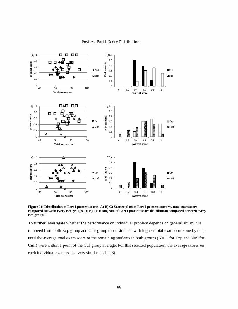
88
Figure 31: Distribution of Part I posttest scores. A) B) C) Scatter plots of Part I posttest score vs. total exam score
compared between every two groups. D) E) F): Histogram of Part I posttest score distribution compared between every
two groups.
To further investigate whether the performance on individual problem depends on general ability, we
removed from both Exp group and Cinf group those students with highest total exam score one by one,
until the average total exam score of the remaining students in both groups (N=11 for Exp and N=9 for
Cinf) were within 1 point of the Ctrl group average. For this selected population, the average scores on
each individual exam is also very similar (Table 8) .
0
0.2
0.4
0.6
0.8
1
40 60 80 100
po
stte
st s
core
Total exam score
Ctrl
Exp
0
0.1
0.2
0.3
0.4
0.5
0.6
0 0.2 0.4 0.6 0.8 1
% o
f st
ud
ents
posttest score
Ctrl
Exp
0
0.2
0.4
0.6
0.8
1
40 60 80 100
po
stte
st s
core
Total exam score
Exp
CInf
0
0.1
0.2
0.3
0.4
0.5
0.6
0 0.2 0.4 0.6 0.8 1
% o
f st
ud
ents
posttest score
Exp
Cinf
0
0.2
0.4
0.6
0.8
1
40 60 80 100
po
stte
st s
core
Total exam score
Ctrl
CInf
0
0.1
0.2
0.3
0.4
0.5
0.6
0 0.2 0.4 0.6 0.8 1
% o
f st
ud
ent
posttest score
Ctrl
Cinf
Posttest Part II Score Distribution
A
B
C
D
E
F

89
212 final hex1 hex2 hex3 Total Exam Score
Ctrl 65.16 ± 2.18 % 65.77 ± 1.95 % 63.22 ± 2.76 % 67.83 ± 2.69 % 65.43±1.70 %
Exp 66.0 ± 2.83 % 68.81 ± 3.13 % 65.73 ± 3.93 % 68.09 ± 4.26 % 66.4±1.93 %
Cinf 63.78 ± 3.16 % 71.78 ± 2.17 % 62.33 ± 3.98 % 67.44 ± 2.70 % 65.96±2.23 %
Table 8: Exam scores for selected population.
When we now plot the correct rate on each question for this selected sub population of students in Figure
32, we find that the correct rate is no longer different for PI-1 and PI-2. Note that 3 out of the 4 students
who scored near zero on Part I are included in this population, which significantly lowers the correct rate
on most problems for this small population.
However, the correct rate for PII-1 and PII-6 remains largely unchanged for this selected population, and
despite the smaller sample size, the correct rate remain significantly different between groups (p=0.003
for PII-1, and p=0.02 for PII-6, fisher’s exact test)
Figure 32: Posttest problem correct rate for selected population with equivalent ability score.
7.3.5 Student Rating of Tutorial and Viewing Data
Given the observed performance differences between the different groups, an important question to ask is
whether the tutorials given to the two control groups are of similar quality as the normal instructional
materials students receive every day. If students in the control group were confused by the tutorials, our
experiment would be an attack on a “straw-man” that we created ourselves.
To answer that question, we will examine two pieces of information. First, we look at students’ rating on
the quality of the multimedia tutorial. The students we recruited in our experiment had been viewing
similar multimedia tutorials as part of the physics 212 course for an entire semester, which provides them
with adequate experience with this type of material to give a reliable rating of their quality.
0
0.2
0.4
0.6
0.8
1
PI-1 PI-3 PI-4 PI-6&7 PI-8
% o
f co
rrec
t an
swer
Ctrl
Exp
Cinf
0
0.2
0.4
0.6
0.8
1
PII-1 PII-2 PII-4 PII-6
% o
f co
rrec
t an
swer
Ctrl
Exp
Cinf
A B

90
Part I Rating Part II Rating
Ctrl 7.73 ± 1.75 8.59 ± 1.18
Exp 8.10 ± 1.48 8.52 ± 1.66
Cinf 8.11 ± 1.75 7.83 ± 1.20
Table 9: Average students' rating of both parts of the tutorial.
All three groups gave almost identical average ratings (~ 8 out of 10) to the first part of the tutorial. The
Ctrl group and Exp group also gave identical ratings to the second part of the tutorial, while the Cinf
group gave a slightly lower (but statistically insignificant, p= 0.23) rating. One student in Cinf group
explicitly commented that the equipotential rings were distracting in this part.
Secondly, we look at the time students spent watching each part of the tutorial. From previous
experiences analyzing students’ interaction with multimedia (and also common sense), we know that if a
student is confused by certain parts of a multimedia tutorial, they will often tend to rewind through that
part and watch it again. Therefore, we could estimate the quality of the tutorial simply by looking at the
total time they spent on watching it. Furthermore, if one particular segment of the tutorial is confusing to
most students, then it would receive more rewinds in total compared to neighboring segments. Therefore,
we will be able to identify which segment of the tutorial they spent the most time watching, simply by
counting the number of times the cursor on the player is dragged pass that segment of animation.
Figure 33: Average number of times students watched every 10s segment of the animated tutorial.
We plot the average number of times each 10s of the tutorial is being watched by students. As can be seen
in Figure 33, the viewing pattern is essentially the same for the three groups of students. In addition, the
beginning and end of tutorial part 1 are the only two sections that received more frequent views than other
0
0.5
1
1.5
2
2.5
3
1 3 5 7 9 11 13 15 17 19 21 23
Ave
rage
nu
mb
er o
f ti
mes
w
atch
ed
Interval (10s)
Part I
Ctrl
Exp
Cinf
0
0.5
1
1.5
2
2.5
3
1 2 3 4 5 6 7 8 9 10111213141516
Ave
rage
nu
mb
er
of
tim
es
wat
ech
ed
Interval (10s)
Part II
Ctrl
Exp
Cinf

91
sections. The beginning of part 1 does not contain any important information, and from our experience
with students the frequent re-watching is most likely due to a number of students who forgot to turn on
the audio or plug in their headphone.
At the end of tutorial part 1, the mathematical expression of the integral is provided to the students. From
previous experience analyzing similar data from students viewing multimedia presentations, we found
that many students tend to re-watch the tutorial whenever a math result appears on screen, probably
attempting to write it down. In fact, we did see a number of students who wrote down the math expression
on their posttest worksheet.
Aside from these two areas, most other areas of the tutorial are viewed only once by most students,
although they are given the opportunity to freely rewind anytime during the experiment. There’s no single
part in any of the three tutorials that attracted or caused a significant number of students to want to or
have to watch it again.
7.4 Discussion
The key observation from the results of this experiment results is that there is a clear difference between
the three groups, on the conceptual understanding of the integral expression of electric potential. Given
that the participants’ content knowledge before the experiment were not significantly different, and their
general learning ability did not seem to correlate with their posttest performance, it is most likely that the
difference in posttest performance is caused by the difference in visual representation design.
Compared to previous experiments on multimedia learning, the differences between the designs in the
current experiment are much smaller. In most of Mayer’s experiments either the representing media or the
time order of presenting the material is different between the groups, and in Schnotz’s experiments,
graphs with completely different geometrical structures were given to different groups.
The fact that differences as subtle as changing the color and motion of equipotential rings can have an
observable effect over a period of ~5 minutes, suggests that we are one step closer to understanding and
identifying the critical factor that determines the effectiveness of computer animation as well as
multimedia instruction design in general. In other words, our new model has enabled us to better harness
the power of visualization enabled by computer technology.
As was mentioned previously, the existing MML models of Mayer and Schnotz make contradictory
predictions as to whether these small differences in visual representation design would lead to any
difference in learning outcome.
92
In addition, neither model was able to provide a satisfactory explanation as to why the control group
designs caused much difficulty in problem solving and knowledge transfer, and why the added
visualization in the EXP group design helped students to overcome these difficulties in a number of cases.
All three versions are designed to comply with Mayer’s seven principles of multimedia designs as well as
our interpretation of these principles would allow. This means that according to Mayer’s MML learning
theory, all three versions should have minimized the extraneous cognitive load, and will not result in
much difference in learning outcomes. Strictly speaking, since the EXP version design contains more
visual elements (color and motion) than the other two, it should require the most cognitive load to process,
which will leave fewer cognitive resources to process the mathematical expression. However, EXP group
students are at least as good as the other group students in constructing the integral expression on all
posttest problems, (even better in some cases (PI-1)), while at the same time significantly outperform the
control groups in other tasks.
Schnotz’s model assumes that students mentally recreate previously learned representation in the form of
a mental model, and read-off information from the model to facilitate reasoning. Vice versa, the mental
model can also incorporate information gained from the semantic network obtained from verbal and
symbolic explanation.
This model of MML might explain part of the difference observed in PII-1, since the information that
electric potential is constant within a conductor is more obvious from the EXP group animation (constant
color), and should be easier to read-off if the representation is recreated.
However, it is not clear why both control groups have almost no success in using their “semantic network”
to acquire the same information. More specifically, since the graphical representation of the posttest
problem is very different from that of the example problem (or the mental model), information from the
mental model cannot be directly applied to the problem. According to Schnotz, students must first “read-
off” information from their mental model, integrate that information into the semantic network, then
examine the figures in the problem based on that information. On the other hand, directly applying
semantic rules to the problem figures requires one less step of cognitive process (Figure 34). Yet, this
presumably more direct pathway resulted in almost no success at all, whereas the more indirect pathway
is significantly more accurate.

93
Figure 34: Schnotz's model's explanation of PII-1. As is shown in the figure, verbal explanation should be more directly
related to the figure.
Schnotz’ model faces more difficulty explaining the results of other problems such as PI-1 and PII-6. In
these problems, completely recreating the previously learned graphical representation will almost
certainly result in wrong answers since the problem context is different from the example. For example, in
PII-6, if one compares the previous graphical representation and the current problem context, the most
obvious difference is the thick shell being replaced by the thin shell. However, this feature is irrelevant to
solving the problem, and likely leads to reasoning such as “there’s no area where the electric field is zero,
so the result won’t change”, which is a wrong answer frequently observed among control group students.
On the other hand, if students are able to properly modify the example representation based on their
semantic network, then the same information is already sufficient to solve the problem. In other words, as
the mental model provides no new information, there is no need to create one. In fact, the solution to both
PI-1 and PII-6 involves either math manipulation or qualitative reasoning. According to conventional
amodal view of cognition, these tasks should be processed predominantly via the semantic network.
Therefore Schnotz’s model would predict that the difference in visual representation will have no effect
on the posttest performance.
In conclusion, neither model was able to identify the cause of difficulty in the design of two control
versions, nor are they able to identify the positive elements in the Exp version design that lead to the
observed improvement on the posttest.
From the perspective of our grounded cognition MML model, the problem with both control group
designs lies in their over-reliance on the S-method to convey physics ideas, while neglecting the P-
94
method. On the other hand, the Exp version overcomes this problem by properly utilizing the P-method to
more effectively activate cognitive resources, resulting in better knowledge construction.
As previously mentioned, the S-method is less effective in teaching since its proper functioning requires
the creator and receiver of the representation to have similar background knowledge, which is almost
never the case in teaching.
In consequence, representation design that relies solely on the S-method can be easily misinterpreted by
students, even if both visual and audio forms of representation are being used. Students’ answers to PII-1
serve as a good example of such misinterpretation: the expression “there is no potential difference inside
the conductor” is interpreted as “there is no potential inside the conductor”.
In contrast with Schnotz’s model (and amodal symbols view in general), grounded cognition refutes the
idea that semantic meaning is more closely related to words or symbols than to perception. Instead,
interpretation of symbolic meaning requires the creation of a simulation which is largely influenced by
background understanding. Therefore, since the participants in the experiment were chosen to have very
similar understanding of the subject, it is likely that a common misinterpretation (zero field means zero
potential) exists among these students.
In comparison, the P-method is much more robust and independent of background knowledge. When not
utilized properly, perceptual features of representation serve as a source of interference to the S-method,
which increases the chance of misinterpretation. In the Exp version, the animation design serves to
activate the perceptual symbol(s) representing the notion of “uniform” and “not change” through the P-
method. Although the geometric structures of the example animation and the correct problem figure are
very different, both of them contain perceptual features that could activate perceptual symbols
representing the concept of “not change” via perceptual inference, such as a patch of uniform color and a
straight line. These inferred perceptual symbols can be directly compared, without involving the language
system. From a grounded cognition perspective, perceptual features are more directly related to the
meaning by sharing part of the same neural circuits, and therefore results in much less misinterpretation.
Aside from low accuracy, another drawback of the S-method is that it is also more expensive in activating
cognitive resources, especially for novices who are not fluent with interpreting the meaning of symbols.
In addition, the need to frequently filter irrelevant perceptual symbols in a low P-value instructional
material further limits students’ cognitive resources that could be allocated to the execution of the S-
method.

95
As a result, students subjected to low P-value instructional materials often cannot activate enough
perceptual symbols to construct a proper simulation for the physics concept. Instead, many irrelevant
surface features of the representation are stored as part of the conceptual understanding (rote learning).
Since these surface features are simply memorized, it is difficult for students to determine whether they
apply to new problem contexts. As a result, students in the control groups are more successful when the
problem context or the format of solution shares more surface features with that of the example, such as
PII-2 and PII-4.
In contrast, when the problem context is very different from the example, students in control groups have
much difficulty in deciding whether certain surface features in the example still apply to the new problem
context.
For example in PI-1, more students in the control groups set the integral limit either to zero or to the inner
surface of the shell (r=a), which are both unnecessary surface features that existed in the example solution.
In PII-6, students in the control groups often focus on the shell being “infinitely thin”, so there is no area
where the E-field is zero, thus concluding that the change in radius will not affect the total potential
difference. However, the thickness of the shell is a feature that is relevant only in the example context
which has a conducting shell, but is not important for the thin insulating shell in the problem context.
On the other hand, the visual representation design of the Exp version utilizes the P-method to activate
more cognitive resources, which at the same time reduces the amount of irrelevant perceptual features that
require active filtering. The net result is that more cognitive resources are activated, which increases the
chance of constructing a proper simulation (grounded cognition equivalence of conceptual understanding)
through studying the material.
In that case, the exact form of the solution is not memorized as an arbitrary fact, but rather as an end
product that is created based on the simulation, or as a method of describing the simulation(s). When
encountering a new problem, the existing simulation is modified based on the problem context.
Modifying previously learned simulation based on text or graph is a basic skill that is required for any
text or figure comprehension task, and should be well mastered by our subjects. As the simulation is
modified to represent the problem context, the solution that is derived from that simulation changes
accordingly, avoiding the inclusion of irrelevant surface features. In addition, since the same simulation(s)
can be described in a number of different ways, students who are describing a simulation will tend to
generate solutions that use more of their own language, and has less surface similarity with the example
solution.
96
Those predictions are most significantly reflected in students’ answers to PII-6. For this problem,there are
two different types of solution. One could either evaluate the integral expression obtained in the previous
problem PII-4 (how each term of the integral change with R), or engage in qualitative reasoning of the
physical situation.
For experts, these two types of reasoning are the two sides of the same coin, and since expert’s physics
knowledge is so tightly bounded to the corresponding mathematical expression, it is sometimes hard for
some experts to notice any difference between the two solutions.
However, for novices who are much less fluent with the math language, we suspect that these two types
of reasoning may reflect different types of thought processes. Since mathematical evaluation can be
performed without much physics understanding, this method should be preferred by those who aren’t able
to construct a proper simulation of electric potential in the problem context. On the other hand, when
students are describing their simulations, they would prefer to describe their thoughts in their most
familiar language, which should be mostly the English language occasionally scattered with math
symbols.
A closer look at students’ answers to PII-6 reveals such a difference. In both control groups, a total of 8
students chose the math evaluation strategy, while only 2 adopted this strategy in the Exp group. In
contrast, 9 students in the Exp group produced correct qualitative reasoning, whereas only a total of 3
students from the other two groups were able to correctly use qualitative reasoning to answer the question.
In addition, the math evaluation required for this problem involves evaluating two terms changing in the
opposite direction, which is a non-trivial task for our subjects. As a result, only 1 out of the 8 students
who adopted this strategy in both control groups successfully came up with the correct answer (this
subject simplified his/her answer to PII-4, leaving her with only one term that is changing). All other
students neglected one of the two terms. One of the two students in the Exp group came up with the
correct mathematical answer. Another possible reason for the high error rate of mathematical evaluation
strategy is that most students likely do not have the corresponding physics model to check whether their
math evaluation made any sense.
On the other hand, the 9 students who gave correct verbal reasoning in the Exp group used rather non-
canonical language such as “the length of the first integral, which has a (Q+q) factor, increased”, or “(the
bigger electric field) would take up more of the integrand”, “k(Q+q) will contribute to more of the
integral”, which is similar to what we had expected from novices describing their simulation.

97
Another benefit of a proper simulation in problem solving is that it enables the appropriate categorical
inference to be activated through the C-method either during the learning stage or during the problem
solving stage.
In order to generate the correct qualitative reasoning for PII-6, a critical step is to notice the simple fact
that accumulating bigger elements over a longer period (or space) will result in a bigger total sum. This
idea is probably a p-prim that is gained from dealing with the accumulation process in everyday life, and
can be activated as a categorical inference through the “ad hoc category” (L.W. Barsalou, 1983) of
“things that can be accumulated”, such as money and effort. When the integral expression of electric
potential is treated as the description of a simulation that represents accumulating electric field along a
path, the appropriate categorical inference can be readily accessed.
Otherwise, if the integral expression is treated merely as a recipe to calculate a number, then it cannot be
categorized as an accumulation process, and the categorical inference cannot be activated even though
students “possess” that knowledge.
Without a proper simulation to support categorization based on structural similarities, the concept of
electric potential is often very naively sorted into the same category as electric field, since they share
many surface feature similarities in their names, math expression, and relevant problem contest. (Some
researchers argue that young children categorize objects based entirely on appearance similarities
(Sloutsky, Kloos, & Fisher, 2007).). Treating electric potential as being very similar to electric field likely
resulted in answers such as “electric potential doesn’t change so that electric field doesn’t change either”,
which is another type of common wrong reasoning among students.
Since students in the Exp group are much more likely to have a proper simulation of the electric potential,
it is not surprising that they are much more likely to come up with the correct qualitative reasoning.
Finally, our model also predicts that in easier cases, rote learning reduces the efficiency of problem
solving since the rote learned rules have to be interpreted as simulations before they could be used for
reasoning.
The form of the current experiment is not designed to demonstrate this effect, since students’ are allowed
to spend as much time as they would like on any problem, and the time on task is not recorded. Therefore,
there is no direct evidence for this prediction.
In summary, the experiment results demonstrate that subtle differences in the design of visual
representation of multimedia material can result in noticeable differences in learning outcomes in physics

98
education. The observed differences can neither be predicted nor satisfactorily explained by existing
MML models. Our grounded cognition MML model attributes the performance differences to the
different P-values of the representation, or in other words, the degree to which each representation utilizes
the P-method of resource activation. The predictions of our model are not only supported by the
difference in posttest scores, but are also in agreement with the types of reasoning observed among
students.
Of course, our MML model cannot explain all the results of the experiment. Especially for part I of the
posttest, several problems did not show significant between group differences. We suspect that several
other factors that are not considered in our model may explain this result. First of all, part I of the tutorial
is given to students immediately after they enter the experiment. Some of the students might still not be in
the right state for learning. In comparison, part II of the tutorial was given to students after they have tried
to solve several related problems, and resulted in a more significant outcome. It has been shown that
problem solving improves the learning of consecutive materials (Schwartz & Martin, 2004).
In addition, both the problems and the tutorial in part I are relatively easier, and are more similar to the
problems and examples students have encountered in class. For example, almost the exact problem of PI-
4 had been used as an example in class. Therefore, we suspect that the memory of similar previous
problems may be interfering with students’ choice on PI-4, which decreases the difference.
Lastly, in order to perform a clinical experiment within reasonable time and cost, we made a number of
compromises that could affect the learning outcome. Three of the major compromises are: 1. We did not
teach the concept anew, but rather offered the tutorial after the concept have already been introduced to
the students. Doing so allows us to use a wider variety of assessment problems following a relatively
short tutorial. Unfortunately, this also means that students could have already gained most of the wrong
ideas in the classroom due to conventional methods of teaching, and will have a harder time overcoming
these misconceptions. 2. The total time of the tutorial is only around 5 minutes, for the purpose of
controlling the total time of the experiment. This makes it harder to induce subtle conceptual changes in
students’ mind. 3. We are restricted to recruiting ~15 subject in each group due to cost restrictions. This
limits the statistical power to identify smaller changes.
However, the fact that we are able to observe some significant between group differences despite of all
those compromises suggests that the impact of P-value on students’ conceptual understanding is quite
significant, and should not be neglected by instructors.

99
8 Experiment 2
8.1 Multimedia Design and Predictions
In experiment 1, we showed evidence that the P-value of instruction could have a significant impact on
students’ understanding of difficult concepts such as electric potential.
However, in introductory physics, only a handful of concepts are as hard and unnatural as the electric
potential. For most concepts, the common level of understanding is somewhere between “total
misconception” and complete mastery. As a result, a more common difficulty faced by students during
problem solving, is to decide which piece(s) of physics knowledge they have learned is relevant to the
problem, especially for a problem that requires multiple pieces of knowledge.
As instructors, we often observe that students fail to activate knowledge that they seemingly possess
during problem solving, especially when the context of the problems is somewhat unfamiliar. (Hammer,
Elby, Scherr, & Redish, 2005) In addition, when a certain problem requires a multi-step solution, it is
especially hard for students to recognize the knowledge that is needed for the intermediate steps of the
problem.
Our model of multimedia learning provides a possible explanation for the origin of such difficulties in
knowledge activation. As was discussed in the section 6.2, a piece of knowledge, such as a physics
equation, can be stored in two different forms. Under successful learning conditions, the knowledge is
interpreted and stored as one or more simulations, while under unsuccessful learning condition, students
engage in rote learning and the physics law is stored as symbols encoding the law.
For easier problems with familiar context and a straight forward solution, knowledge stored in both forms
are sufficient, which leads to the impression that students “possess” that knowledge. However, when
faced with a problem of unfamiliar context, knowledge stored as simulations having a much higher
probability of being properly activated than those stored as symbols. For problems that require multiple
pieces of knowledge, the human brain can easily generate multiple simulations simultaneously (Lawrence
W. Barsalou, 2009), thereby allowing more pieces of knowledge to be considered for the solution. In
contrast, our brain’s ability to activate and interpret multiple symbolic rules is rather limited, probably
because the ability to interpret symbols is evolution wise a very new trick learned by the brain. Therefore,
thinking of physics rules as symbols significantly limits the brain’s ability to construct multi-step
solutions.
100
As was discussed in previous chapters and supported by the previous experiment, instructions with
positive P-values could facilitate the construction of new simulations and avoid rote learning. Therefore,
in addition to improving conceptual understanding and transfer for difficult concepts, increasing the P-
value of instruction should also result in increased probability of activating proper knowledge during
problem solving, especially for problems requiring multiple pieces of easier knowledge.
8.1.1 Topic: Simple Capacitance Circuit
In experiment 2, we will test this theoretical prediction in the context of simple capacitance circuit
networks. We chose the capacitance circuit as our topic for two major reasons. First of all, the behavior of
simple capacitor circuits are determined by a set of simple rules, describing the relation between charge,
voltage and capacitance of capacitors connected either in parallel or in series. Each rule is very simple by
itself, can be expressed in one short sentence, and only requires middle school math to interpret. All these
features encourage rote learning under low P-value condition. On the other hand, it is easy to create
problems that require three to four different steps to solve, for which students with proper simulation will
have an advantage. Therefore, simple circuits serve as an ideal testing ground for our predictions.
Secondly, we chose DC capacitor circuits over resistor circuits or other circuits, simply because there is
no current in the circuit and only static charges are stored on the capacitors. Proper animation of electric
current is technically much harder to create than static charges, and could easily carry unwanted visual
artifacts.
Therefore, we chose to use simple capacitor circuit problems as the testing ground for exploring the
relation between P-value of instruction and students’ problem solving ability.
8.1.2 Representation Design
In order to increase the P-values of the instructional materials on capacitance circuits, we
examined the conventional representation for every one of the rules that determines the state of the
capacitance circuit, and redesigned certain aspects of the representation with low or negative P-values.
The set of rules for capacitor circuits describes the relation between three physics quantities:
capacitance C, voltage V, and charge Q, for series and parallel connections. All other rules can be derived
from the basic equation Q=CV, and the definition of parallel and series connections.
For the purpose of demonstrating the visual representation design, we will start with the ones
having simpler visual representations, and discuss the basic rule of Q=CV at the end. However, it must be
pointed out that the actual order by which the rules are presented to the students is reversed, starting with
the basic capacitor equation Q=CV.

101
8.1.2.1 Capacitance
For capacitance C, the basic rule is that the equivalent capacitance of two parallel capacitors is
bigger than any one of them, and the equivalent capacitance of two series capacitors is smaller than any of
them. Mathematically, the rule can be expressed as:
Conventionally, visual representation accompanying this rule is very simple, as shown below:
Figure 35: Conventional representation of equivalent capacitance. Shown here is a schematic illustration of the
conventional representation of equivalent capacitance for series and parallel capacitance. In the actual tutorial, the
parallel and series cases are shown one at a time, and the diagram on the left would fade away while being replaced by the
diagram on the right.
Aside from showing the topology of series and parallel connection, the P-value of this
representation is low because of the following two reasons.
First of all, all the capacitors are drawn to the same size, regardless of their actual capacitance.
According to the PSS framework, the same neural circuits responsible for judging the perceived size of
the symbols are also involved in processing the magnitude of their represented value. Such interference
between perceived size and represented magnitude is well known for math symbols. (Henik & Tzelgov,
1982) Therefore, we have good reason to believe that the perception of identical sizes of two capacitor
symbols can interfere with simulating (in other words understanding) one capacitor having a bigger
capacitance than the other

102
Secondly, the idea that two capacitors can be viewed as one equivalent capacitor is not
perceptually represented. Students have to generate the simulation of the two capacitors being replaced by
one larger or smaller capacitor from scratch, which is both cognitively demanding and error prone.
Therefore, in our redesigned visual representation, the physical size of the capacitor symbol is
used to indicate the relative value of its capacitance. (For real parallel plate capacitors, the surface area of
the plate is also proportional to its capacitance.) In addition, the verbal explanation of “equivalent
capacitor” is accompanied by animations showing the two capacitors being gradually merged together,
into either a larger or a smaller capacitor. We believe that such an animation will make it easier for
students to think about equivalent capacitance in different topologies.
Figure 36: Screen shots of perceptually enhanced design for equivalent capacitance. Above: Screen shots of the animation
demonstrating two parallel connected capacitors gradually merging into one larger equivalent capacitor. Below: Screen
shots of the animation demonstrating two capacitors connected in series merging into a smaller equivalent capacitor.
Notice that the physical size of the capacitor symbols are used to represent the magnitude of their capacitance.
8.1.2.2 Voltage
Voltage across two capacitors connected in parallel are the same, and voltage across two
capacitors connected in series are inversely proportional to their capacitance. The mathematical
expression for this rule could be expressed as:
Parallel:

103
Series:
Conventionally, the visual representation accompanying this rule simply indicates V1 and V2
above the symbols of capacitors (Figure 37). The P-value of such a representation is predicted to be rather
low, because the symbols above the capacitor may leave the impression that voltage is stored on the
capacitor, in much the same way as charges are being stored on the capacitor, and the wires connected to
the capacitors are irrelevant to the voltage. In fact, voltage is uniform over a segment of circuit, and the
voltage drop across the capacitor, represented by the V symbols, reflects the difference in voltage
between two segments separated by the capacitor.
Figure 37: Conventional representation of voltage across capacitors.
In order to properly represent the concept of voltage drop, we redesigned the visual representation,
using color and thickness of the wires and plates to represent the voltage of that circuit segment, which
shows a radical change across capacitors (Figure 38). Under such a representation, the rule for the parallel
case becomes visually obvious, and the rule for the series case seems more intuitive.
The sizes of the capacitors are still used to indicate its capacitance, and the color/thickness
difference across the capacitor is used to indicate the magnitude of potential drop. The color and thickness
are chosen so that not only the difference is obvious, but the magnitude of difference can also be easily
detectable.

104
Figure 38: Perceptually enhanced representation of voltage across capacitors. Difference in colors and line thicknesses are
used to represent difference of potential in segments of circuits.
8.1.2.3 Charge
In capacitor circuits, parallel capacitors store charges proportional to their capacitances, while
series capacitors store the same amount of charge. Mathematically, this can be expressed as:
Parallel:
Series:
The conventional representations of the charge rule is much like that of the voltage rule, except
that occasionally, plus and minus signs are being added to the capacitors to indicate the signs of the
charges.
Figure 39: Example of conventional charge representation.

105
The P-value of this visual representation is not as low as the representation for voltage, since
charges stored are local valued of the elements. However, the P-value is still around zero, since there are
no perceptual features that correspond to the different magnitudes of the stored charges.
In addition, this representation also yields a very low P-value when it comes to teaching the proof
of these rules. For example, the reason that capacitors connected in series have the same charge is simply
because the two plates in the middle is essentially a neutral piece of metal, and therefore must have equal
charges on both sides. Under the current representation, no perceptual feature serves to facilitate this
understanding.
Therefore, in order to improve the P-value of this representation, we used a number of small
charge symbols to represent charges stored on each plate of the capacitor. The relative number of the
charges reflects the relative amount of charge stored on the plates. In addition, when introducing the
series capacitors case, the charges are created in pairs from the center of the middle segment, to facilitate
the simulation that there must be equal amount of charges on each plate of the capacitor.
Figure 40: Example of the perceptually enhanced charge representation. The relative number of the charge symbols
corresponds to the relative magnitude of charge stored.
8.1.2.4 The Capacitor Equation
For a capacitor circuit, the basic equation that connects voltage, charge and capacitance is the
capacitor equation:
From this equation one could easily derive the voltage and charge rules mentioned above.
Under conventional representation, none of the magnitudes of the three variables are perceptually
represented, and students have to generate the corresponding simulation on their own. Under our

106
redesigned representation, relative magnitudes of the variables can be directly perceived, which should
facilitate the proper construction of a simulation.
Figure 41: Two different types of visual design for the capacitor equation. Left: conventional design. Right: Perceptually
enhanced design.
In this experiment, each individual change of the design is relatively simple, some even trivial.
There’s little doubt that if only one or two of these rules are being taught and tested with conventional
representation, a normal student could easily overcome the deficits of its low P-value, and construct a
proper simulation through active thinking. In addition, even if the student practiced rote learning during
the learning phase, he would have little problem translating the symbols into a simulation during the
problem solving phase. The small “rule space” made it possible for students to traverse the entire rule
space for every problem. This means that for simpler cases, the possible impact of P-value on learning
outcome, if any, would be hard to measure.
However, we believe that when the entire set of rules is taught at the same time, the cumulative
cognitive load required to generate proper simulations for each of them becomes quite demanding. In
addition, the symbolic representation of each individual rule is so simple and easy to memorize, that it
likely invites shallow, rote learning when the P-value of the instruction is almost zero. Improving the P-
value of each representation should encourage the generation of simulation, and serve to offset the bias
towards rote learning.
On the other hand, with a larger “rule space”, rote learning students can no longer traverse the
entire space to solve assessment problems, especially problems that involve multiple steps. Since
translating a single symbolic rule into a simulation is cognitively demanding, translating two or more
rules in series is a daunting task for students, let alone having to determine which rule to translate. Data
from past final exams have shown that circuit problems involving more than three steps have significantly
lower averages than more straight forward problems.

107
In contrast, the human brain is well evolved to generate multiple simulations in series, or even in
parallel. As mentioned in chapter 6.2, physics rules stored as simulations are not only cognitively cheaper
to activate, but also more likely to be activated under the right context. Therefore, the enlarged “rule
space” provides a much better chance for us to detect rote learning among students.
In conclusion, we believe that although each individual change in visual representation only
brings about a small effect that is hard to identify, the cumulative effect of all the changes will be
measurable with multiple step problems.
8.2 Methods and Implementation
8.2.1 Procedure
The overall procedure of the current experiment is almost identical to that of Experiment 1. The only
difference is that in the current experiment, we created two, instead of three, different versions of
animated tutorials, because the perceptual-rich design of the current instruction does not introduce any
extra visual elements.
8.2.2 Animated tutorial
Two versions of a short (~4 minutes) animated tutorial were created, one for each visual
representation design. Both versions share the same audio narration script, which was written before the
creation of the animation. The audio script was created following the same procedure as in experiment 1.
Nowhere in the audio script do we mention the relationship between visual elements and the
corresponding physical values, such as the size of the capacitor symbol and their capacitance.
The tutorial consists of two parts. In the first part, the basic rules are introduced. The first part is
divided into two sections. The first section introduces the capacitor equation Q=CV, and the second
section introduces the voltage distribution and charge distribution rules. In the second part of the tutorial,
the capacitor circuit problem shown below was solved as an example. Similar to experiment 1, the current
tutorials are also developed as a review tool to help students prepare for the final exam. Therefore, the
derivation of the capacitor equation is not included in the tutorial, nor do we mention the capacitance
equation C= ε0 A/d, which is not related to the problems.

108
Figure 42: Example problem used for the second part of the tutorial. The problem asks when C2 is doubled, how will the
voltage and charge change on the two capacitors.
Animation was first created for the perceptually enhanced version due to technical complexity. A
traditional representation was then created by eliminating the added visual effects.
However, while creating the traditional representation version of the tutorial, we found that for
most of the time, the screen displays a static picture due to lack of a visual representation for voltage,
charge and capacitance. This violates Mayer’s multimedia learning model, which predicts that words
should be linked with appropriate visual counterparts for best learning outcome. However, in the
traditional representation, when the narration says: “under the same voltage, a larger capacitor stores more
charge”, the screen displays a static picture of a capacitor, a battery, and an equation during the whole
time. Therefore, one could argue that the words in this sentence have no corresponding visual counterpart
to be linked to.
To create a conventional representation version of the tutorial that complies with Mayer’s
principles, but does not facilitate the generation of a simulation, we chose to animate the size of the
symbols in the equation. For example, the above sentence corresponds to the enlarging of the variables Q
and C in the equation as shown below:
This animation is, by common sense, unquestionably relevant to the meaning of the verbal
sentence, and is visually clear and simple. Therefore, Mayer’s model predicts that it will likely be linked
with the sentence, and improve learning outcome.13
However, from a grounded cognition perspective, such animation would encourage rote learning
by bringing the focus onto the symbolic equation, rather than the physics process that the equation
13
According to Mayer, online text with audio narration is not optimal for learning. However, talking about an equation without writing it is completely absurd. In addition, as previously discussed, math expression lies on the boundary of picture and text. By introducing symbol animation, the equation shares even more commonalities with pictures than with text.
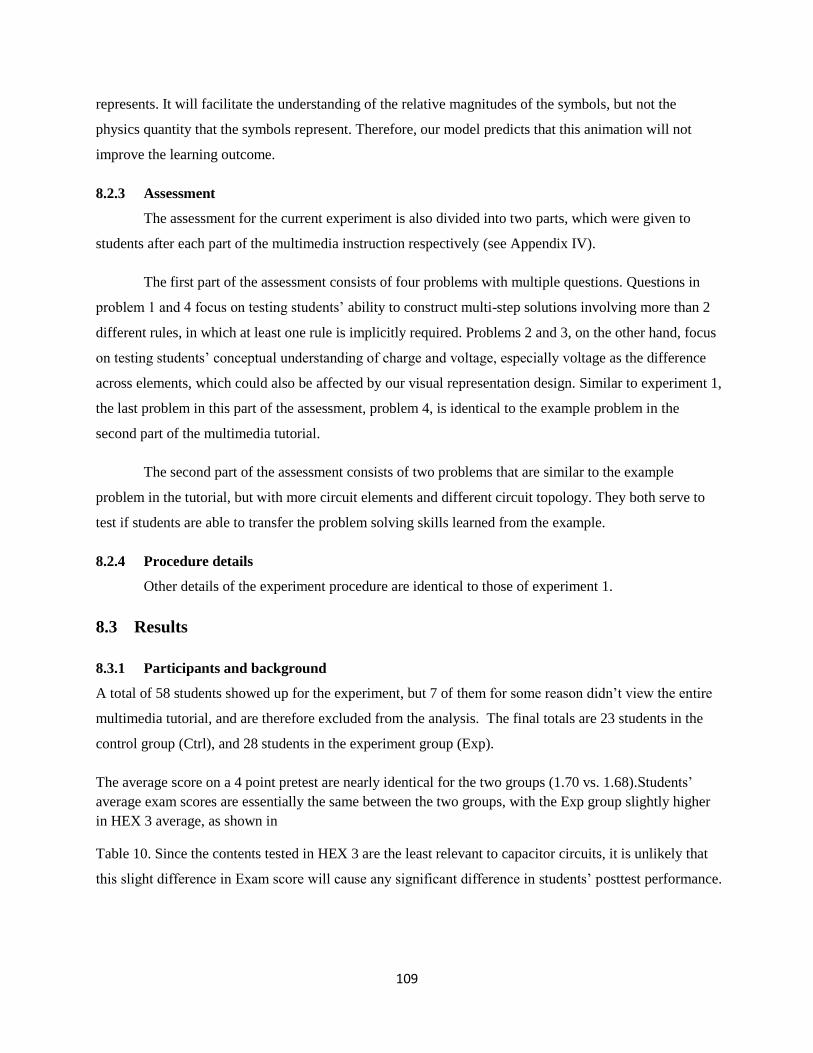
109
represents. It will facilitate the understanding of the relative magnitudes of the symbols, but not the
physics quantity that the symbols represent. Therefore, our model predicts that this animation will not
improve the learning outcome.
8.2.3 Assessment
The assessment for the current experiment is also divided into two parts, which were given to
students after each part of the multimedia instruction respectively (see Appendix IV).
The first part of the assessment consists of four problems with multiple questions. Questions in
problem 1 and 4 focus on testing students’ ability to construct multi-step solutions involving more than 2
different rules, in which at least one rule is implicitly required. Problems 2 and 3, on the other hand, focus
on testing students’ conceptual understanding of charge and voltage, especially voltage as the difference
across elements, which could also be affected by our visual representation design. Similar to experiment 1,
the last problem in this part of the assessment, problem 4, is identical to the example problem in the
second part of the multimedia tutorial.
The second part of the assessment consists of two problems that are similar to the example
problem in the tutorial, but with more circuit elements and different circuit topology. They both serve to
test if students are able to transfer the problem solving skills learned from the example.
8.2.4 Procedure details
Other details of the experiment procedure are identical to those of experiment 1.
8.3 Results
8.3.1 Participants and background
A total of 58 students showed up for the experiment, but 7 of them for some reason didn’t view the entire
multimedia tutorial, and are therefore excluded from the analysis. The final totals are 23 students in the
control group (Ctrl), and 28 students in the experiment group (Exp).
The average score on a 4 point pretest are nearly identical for the two groups (1.70 vs. 1.68).Students’
average exam scores are essentially the same between the two groups, with the Exp group slightly higher
in HEX 3 average, as shown in
Table 10. Since the contents tested in HEX 3 are the least relevant to capacitor circuits, it is unlikely that
this slight difference in Exam score will cause any significant difference in students’ posttest performance.

110
HEX1 HEX2 HEX3 Final
Ctrl 72.91±2.25 75.13±3.30 74.17±2.60 74.43±2.74
Exp 73.21±1.50 73.86±2.61 78.00±1.99 75.10±2.54
Table 10: Average exam score of students in both groups. Exam performance is measured by percentage rank in class.
8.3.2 Posttest problem types and grading scheme
The entire posttest consisted of 7 problems, 5 in part I and 2 in part II. Among these problems, five of
them (PI-1-1, PI-1-2, PI-4, PII-1, PII-2) require students to write an explanation for their choice or their
answer. For these four problems, scores of 0-3 are assigned based on both the answer and the quality of
their explanation, according to the rubric introduced in the previous experiment.
Among these four problems, PI-4 contains two highly correlated questions that measure student
understanding as a whole. The two questions are graded as one problem and assigned a total grade of 0-3.
Similarly the three questions in PII-2 are also graded as one problem.
All five problems are graded by two graders independently. During the grading process the graders are
unaware of the group assignment of each student. After some discussion, both graders and are able to
agree on the score given to each problem to within 1 point. The number of different scores assigned is less
than 25% of the population in each group for any problem. The only exception being P2-2, where the two
graders differ on half of the gradings. However, the majority of difference is between 0 and 1 points,
(except for 2 cases in Ctrl group and 3 cases in Exp group). As can be seen in the following analysis,
these differences have no significant impact on any of the following analyses.
Since some of the explanations given in the posttest are fairly ambiguous, the average score of both
graders are used in calculating the total score to prevent systematic bias from an individual grader.
For the other two problems, PI- 2 asks students to choose the correct reasoning among five possible
choices, and therefore requires no further explanation. Therefore, students are assigned 3 points if they
pick the correct answer, and 0 if not.
PI-3 is a quantitative problem similar to the ones students have seen on exams. The problem consisted of
three related questions, and students are given 1 point for giving the correct answer to each of the three
questions, so that the entire problem is also worth a total of 3 points. The students’ calculation process is
not considered during grading, since most of the students didn’t write down their complete calculation
process.

111
Since there is no ambiguity to the answers of these two problems, they are graded by one grader.
8.3.3 Posttest Performance
The average total scores for both parts of the post test showed no difference between the two groups, as
shown in the table below.
Part I Part II
Ctrl 41.30±5.05% 35.87±5.60%
Exp 40.23±3.79% 32.14±4.63%
Table 11: Overall posttest performance of students. Scores are reported as percentage of total points available.
However, some individual questions did show some between group differences. As is shown in Figure 43,
the percentage of students having a completely correct answer (3 points) is quite different for each
individual problem in the current experiment, which is very different from the previous experiment in
which most problems showed a similar trend.
One problem, PI-4 showed a significant between group difference. Namely, Exp group students
outperformed the Ctrl group students(p=0.03 one tailed fisher’s exact test) 14
. In PI-2, a slightly larger
fraction of students in the Ctrl group made the correct choice (p=0.13 one tailed fisher’s exact test).
Four of the problems, PI-1-1, PI-1-2, PII-1 and PII-2, seem to be too hard for students, with less than 15%
of students in each group scoring 3 points on these problems.
Figure 43: Percentage of correct answer on each individual problem.
14
For P1-4, there are only 2 cases in the Ctrl group and 1 case in the Exp group where one of the graders assigned 2 points and the other assigned 3 points to the answer. Using the grading of either grader will not change the results.
0
0.1
0.2
0.3
0.4
0.5
0.6
0.7
0.8
P1-1-1 P1-1-2 P1-2 P1-3 P1-4 P2-1 P2-2
% o
f an
swer
s =
3
Ctrl
Exp

112
Interestingly, the background dependence on the two problems that showed some difference is drastically
different. PI-2 seems to be highly dependent on background knowledge. As shown below, those who
made the correct choice on P1-2 have significantly higher exam scores on almost every exam than those
who didn’t make the correct choice. This is true for both the Ctrl group and the Exp group.
Figure 44: Exam scores of those who made the correct choice on PI-2 vs. those who didn’t.
On the contrary, those who scored 3 points on PI-4 showed no dependence on exam scores. In fact, as
shown in Figure 45, those who scored less than 3 points seem to have slightly higher average exam scores
than those who scored 3 points. We couldn’t make the same plot for the Ctrl group since only one student
in the Ctrl group scored 3 points on this problem.
Figure 45: Exam scores of students who scored 3 points on PI-4 vs. those who didn’t. The plot is made for students in the
Exp group only.
For the four harder problems, (PI-1-1, PI-1-2, PII-1, PII-2), less than 15% of the students scored3 points
(less than 30% >=2 points) in each group. For these problems , we would like to know if the difference in
multimedia design has caused any impact on some intermediate steps that may not have been reflected in
the scores, since all these problems require multiple steps to correctly solve.
PI-1-1 and PI-1-2 ask the students to explain what would happen to the properties of a simple two
capacitor circuit, if a third capacitor C3 is added to the circuit in two different ways. (see Figure 46)
0
20
40
60
80
100
HEX1 HEX2 HEX3 Final
Ctrl Group
P1-2 = 3
P1-2 < 3
0
20
40
60
80
100
HEX1 HEX2 HEX3 Final
Exp Group
PI-2 = 3
PI-2 < 3
0
20
40
60
80
100
HEX1 HEX2 HEX3 Final
Exam
% s
core
P1-4 = 3
P1-4 < 3

113
Figure 46: Illustration of PI-1-1 and PI-1-2. A new capacitor C3 is added to the circuit in two different ways. For more
details see the actual posttest in the appendix.
Correctly solving this problem requires students to treat two or more capacitors as one equivalent
capacitor. When we look at how students chose which capacitors to group together, we found an
interesting difference between the two groups.
In PI-1-1, students are asked to compare the voltage on C2 in the two final circuits. 14 and 13 students
scored > 1 points in the Ctrl and Exp group respectively, which means that their written explanation is
interpretable, and both graders agree that they contain some degree of understanding.
Figure 47: Illustration of the problem solving strategy adopted by some students in the Exp group. Capacitors considered
as one equivalent capacitor are circled in red.
In the Exp group, 5 students unambiguously indicated that they treated C1 and C3 as one equivalent
capacitor in both circuits, and indicated that the difference in capacitance between these equivalent
capacitors is the cause for the difference in voltage on C2. Among those 5 students, none of them wrote a
clear enough explanation so that both graders could assign 3 points. In addition, 2 of them made
subsequent mistakes causing them to choose the wrong answer, resulting in receiving only 1 point. Both
graders independently identified all the students that used this approach, and agreed on all the 5 cases
reported here.
In contrast, none of the 14 students who wrote understandable reasoning in the Ctrl group used this
approach. Although some treated C1 and C3 in circuit A as one equivalent capacitor, none of them treated
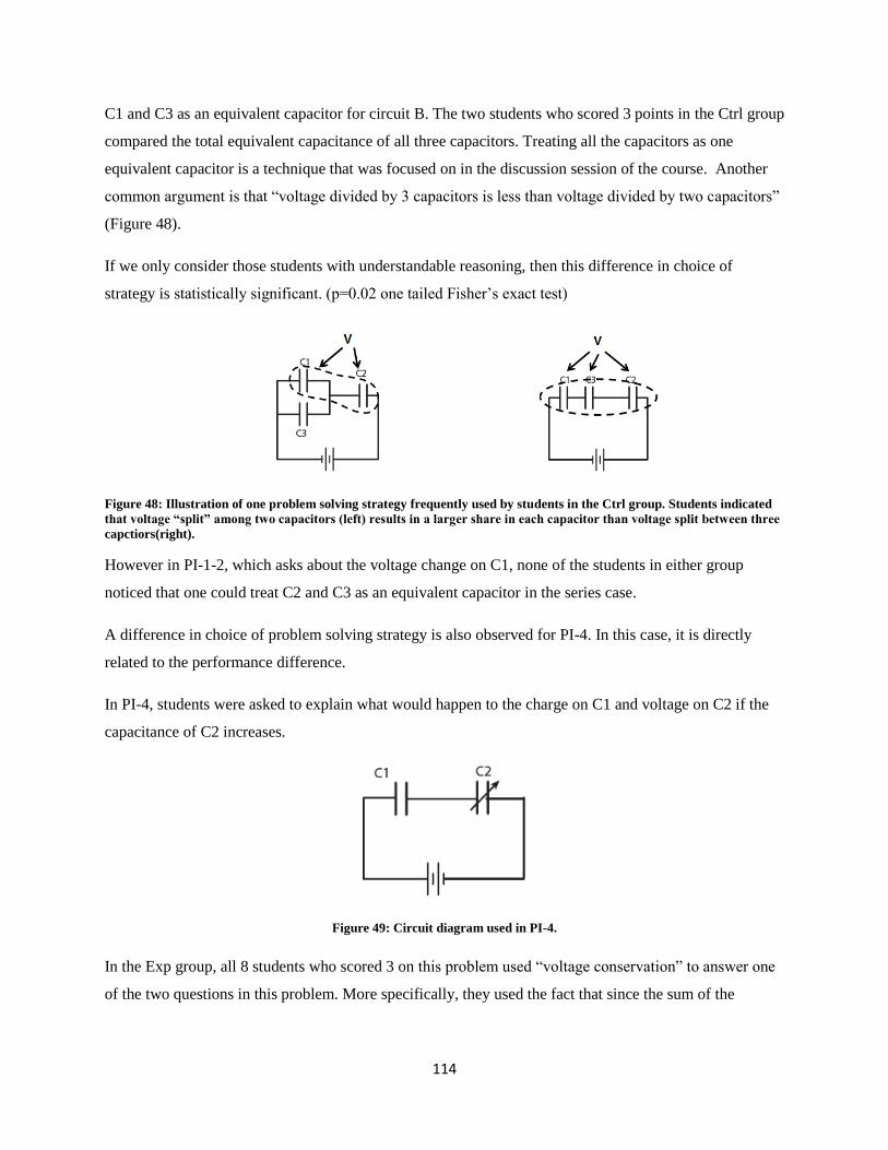
114
C1 and C3 as an equivalent capacitor for circuit B. The two students who scored 3 points in the Ctrl group
compared the total equivalent capacitance of all three capacitors. Treating all the capacitors as one
equivalent capacitor is a technique that was focused on in the discussion session of the course. Another
common argument is that “voltage divided by 3 capacitors is less than voltage divided by two capacitors”
(Figure 48).
If we only consider those students with understandable reasoning, then this difference in choice of
strategy is statistically significant. (p=0.02 one tailed Fisher’s exact test)
Figure 48: Illustration of one problem solving strategy frequently used by students in the Ctrl group. Students indicated
that voltage “split” among two capacitors (left) results in a larger share in each capacitor than voltage split between three
capctiors(right).
However in PI-1-2, which asks about the voltage change on C1, none of the students in either group
noticed that one could treat C2 and C3 as an equivalent capacitor in the series case.
A difference in choice of problem solving strategy is also observed for PI-4. In this case, it is directly
related to the performance difference.
In PI-4, students were asked to explain what would happen to the charge on C1 and voltage on C2 if the
capacitance of C2 increases.
Figure 49: Circuit diagram used in PI-4.
In the Exp group, all 8 students who scored 3 on this problem used “voltage conservation” to answer one
of the two questions in this problem. More specifically, they used the fact that since the sum of the
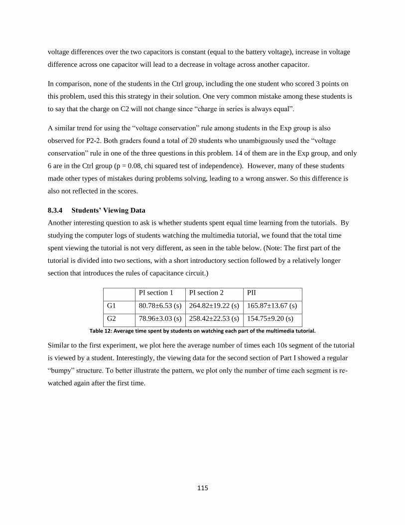
115
voltage differences over the two capacitors is constant (equal to the battery voltage), increase in voltage
difference across one capacitor will lead to a decrease in voltage across another capacitor.
In comparison, none of the students in the Ctrl group, including the one student who scored 3 points on
this problem, used this this strategy in their solution. One very common mistake among these students is
to say that the charge on C2 will not change since “charge in series is always equal”.
A similar trend for using the “voltage conservation” rule among students in the Exp group is also
observed for P2-2. Both graders found a total of 20 students who unambiguously used the “voltage
conservation” rule in one of the three questions in this problem. 14 of them are in the Exp group, and only
6 are in the Ctrl group (p = 0.08, chi squared test of independence). However, many of these students
made other types of mistakes during problems solving, leading to a wrong answer. So this difference is
also not reflected in the scores.
8.3.4 Students’ Viewing Data
Another interesting question to ask is whether students spent equal time learning from the tutorials. By
studying the computer logs of students watching the multimedia tutorial, we found that the total time
spent viewing the tutorial is not very different, as seen in the table below. (Note: The first part of the
tutorial is divided into two sections, with a short introductory section followed by a relatively longer
section that introduces the rules of capacitance circuit.)
PI section 1 PI section 2 PII
G1 80.78±6.53 (s) 264.82±19.22 (s) 165.87±13.67 (s)
G2 78.96±3.03 (s) 258.42±22.53 (s) 154.75±9.20 (s)
Table 12: Average time spent by students on watching each part of the multimedia tutorial.
Similar to the first experiment, we plot here the average number of times each 10s segment of the tutorial
is viewed by a student. Interestingly, the viewing data for the second section of Part I showed a regular
“bumpy” structure. To better illustrate the pattern, we plot only the number of time each segment is re-
watched again after the first time.

116
As can be seen from the plot for the second section
of Part I, there are three clear “peaks” in the Ctrl
group, and two in the Exp group. When we look at
the tutorial, the center of the peak corresponds to the
time when the conclusion of a rule, such as
“capacitors in series have the same charge” is
introduced, and the equation such as Q1=Q2 is shown
on the screen. The troughs in between correspond to
the explanation of the rule. This is quite
understandable since students often go back in the
tutorial to verify the equation they use during
problem solving.
The most significant difference between the two
groups is that the Exp group completely misses the
third peak. When looking at the tutorial, we found
that the center of the third peak corresponds to the
equivalent capacitance rule for series capacitors,
namely “the equivalent capacitance of two capacitors
in series is smaller than either C1 or C2.”
When looking at the viewing data for each student,
we found that some students re-watches the tutorial
much more than others, and therefore, these students
have a larger impact on the average viewing data. To
account for that effect, we plot in Figure 51 the fraction of students who chose to view every 10 second
segment more than once. In other words, every student who chose to view one segment more than once
contributes equally to the final data.
On this graph, there is still a clear difference between the two groups starting from 110s and ends at 150s
in section 2 of Part I. During this time span, two rules are being introduced. At around 110 second, the
“voltage conservation” rule mentioned above is introduced, and at around 150 second, the “equivalent
capacitance of series capacitors is smaller” is introduced. A much smaller fraction of students in the Exp
group chose to watch these two parts for a second time.
Figure 50: Average number of times each 10s interval of the tutorial is been re-watched.

117
Interestingly, students in the Exp group are more
likely to use those two rules that they do not watch
again in problem solving. As mentioned before, in PI-
4 and PII-2, Exp group students are more likely to use
the “voltage conservation” rule in their solutions, and
in PI-1-1, only those in the Exp group used the
“equivalent capacitance of series capacitors is smaller”
rule.
8.4 Discussion
The main focus of this experiment is to test whether a
difference in visual representation design could have
any impact on knowledge activation and execution of
abstract rules.
According to existing theories, abstract rules such as
“capacitors connected in series have the same charge”
are comprehended almost exclusively through abstract
semantic rules by the brain, in much the same way as
executing a line of computer code such as : if
(connected in series) then (charge1 = charge 2).
Since the semantic system was thought to operate
independently from perceptual domains, visual
representation should do no more than provide
information for judging whether the two capacitors
are connected in series, and have no impact on the actual execution of the “if…then…” clause, nor should
it have any impact on the activation of this knowledge, as long as it shows two capacitors connected in
series.
On the other hand, grounded cognition argues that these rules are represented by perceptual simulation(s).
Our grounded cognition based MML model predicts that increasing the P-value of a visual representation
will increase the chance of creating the proper simulation that represents the rule, and thereby reduce rote
learning. Since our brain is much better at processing simulation(s), learning the proper simulation instead
of memorizing the written form of the rule brings a number of benefits during problem solving, such as
easier and more accurate knowledge activation, and lower cognitive cost for execution.
Figure 51: Percentage of students re-watching each 10s interval of the tutorial.

118
In the experimental results, we found some evidence supporting these predictions.
In PI-4 and PII-2, students in the Exp group have a much higher chance of activating the “total voltage
conservation” rule. Notice that the figure used in both problems (Figure 52) are very similar to the ones
used in the Ctrl group design, with equal size capacitor symbols, and uniform black lines. If visual
features are compared independent of semantic meaning, then the problem figure should favor the Ctrl
group for knowledge activation, as they look more similar. On the other hand, from a grounded cognition
perspective, reading the problem text activates a set of perceptual symbols (such as “big” and “small”)
that are combined with the perception of the figure to form a simulation representing the problem context.
The EXP group animation design activates a similar set of perceptual symbols via the P-method, while
the Ctrl group design leads students to memorize the equation “V=V1+V2”, which is less similar to the
problem context. Therefore, on a simulation level, the Exp group design will facilitate knowledge
activation.
In PI-1-1, only students in the Exp group were able to treat C1 and C3 in series as one equivalent
capacitor, and notice that the capacitance difference with C1 and C3 in parallel causes the voltage
difference on C2.
Figure 52: From left to right: Figure used in the assessment (PI-4), representation for voltage conservation rule used in
Ctrl group design, the same representation used in Exp group design
This strategy is particularly interesting since it requires students to hold at least two factors in working
memory at the same time: the equivalent capacitance of two capacitors is bigger in parallel and smaller in
series (or at least they change in opposite directions), and that the change in capacitance in one part of the
circuit affects the voltage difference in other parts of the circuit (voltage conservation rule). Furthermore,
this strategy requires students to consider both circuits at the same time.
In comparison, other solutions provided by students are cognitively cheaper. For example, most students
compared each new case with the original case separately, some even used different strategies for each
case. This allows them to consider one case at a time. The only other strategy that involves directly
comparing the two cases is to state that the voltage split between two capacitors is bigger than the voltage
split between three capacitors, which apparently requires less cognitive load.

119
Therefore, assuming that students’ working memory have approximately equal capacities, it seems that
some students in the Exp group are able to execute certain abstract rules at a cheaper cognitive cost.
Student’s time logs for viewing the multimedia tutorial may also be an indication that enhancing the P-
value improves comprehension of the content.
When interpreting these data, we adopt two simple assumptions. First, we assume that the major cause for
watching a segment more than once is either because students had difficulty comprehending the material
in the first watch, or that they would like to confirm the details of a result before using it in problem
solving. Accordingly, students tend not to look at certain parts of the tutorial either because they think
that the content is obvious, or that they do not think it is useful for problem solving.
The second assumption is that if a significant number of students choose to re-watch a certain segment
more than once, then that segment is relatively difficult (or relevant to problem solving) for all students,
even for those who didn’t choose to re-watch it. In other words, individual differences among the subjects
are only quantitative, but not qualitative.
If we acknowledge these two assumptions, then the conclusion is quite obvious. The fact that most
students in the Exp group didn’t watch the “voltage conservation” rule and the “equivalent capacitance”
rule for a second time suggests that these two rules seem obvious to them, and there is no need to re-
confirm these rules when applying these rules to problem solving.
Admittedly, the difference in posttest performance between the two groups is not as significant as we had
expected. One obvious cause for this is that many of the problems (4 out of 7) turns out to be too hard for
most students, leaving us with insufficient problems to measure the difference.
In addition, we think that several different factors, such as the design of the experiment and assessment,
as well as an underestimation of the interference from students’ prior knowledge, may have also
prevented us from observing a more significant effect.
First of all, it is intrinsically difficult to measure differences in the cognitive cost of knowledge activation
and rule execution. These differences are most easily measured under high cognitive load situations, such
as solving a multiple-step problem, so that those who require more cognitive resources to activate
knowledge or to execute a rule will fail to solve the problem. However, if the problem is too hard, it could
exceed the capability of students in both groups. If the problem is too easy, then those in the Ctrl group
could also solve the problem by thinking a little harder. Most problems in our experiment seem to be
120
either too hard or too easy, showing that it is hard to find the right problem which inflicts the right amount
of cognitive load on students.
Secondly, in a multistep problem, the differences in knowledge activation and rule execution may be
reflected in one or two intermediate steps, but not on the final result, since under a high cognitive load
situation, students are more likely to make various types of careless mistakes. However, in many cases,
students’ explanations of their reasoning are hard to interpret, even though we explicitly asked them to
clearly write down their answers. This may be partly due to the fact that students are hardly ever asked to
put down their qualitative reasoning for their answer, be it in exam, homework, or quizzes. Therefore,
they are not well trained at all to clearly demonstrate their thought processes.
The results reported in the current work include only those cases for which both graders find the answers
unambiguously indicating one type of problem solving strategy. We did find a number of cases where we
suspect that the subject had adopted a certain strategy, but were unable to determine because of the
ambiguous verbal explanation. The ambiguity in explanation is especially severe for the current
experiment, since most problems require students to explain multiple steps of reasoning. As was already
seen in the previous experiment, students tend to prefer writing short answers instead of a complete
explanation.
Finally, in this experiment we tried different problem formats to determine which format is the most
suitable for detecting the intended effect. Therefore, some problem formats might be unsuitable for our
purpose. For example, PI-3 is a calculation task, for which students received frequent training on similar
tasks throughout the course. For this particular problem we find that students often use knowledge not
covered in our tutorial, such as Kirchoff’s voltage rule, to solve the problem. Therefore we suspect that
their performance on this problem may not reflect their learning from the current tutorial. In addition,
students’ description of their calculation process is even more unreadable than their verbal explanations.
So this particular problem format turns out to be unsuitable for our purpose.
In addition to problems in experimental design, we found that students’ prior misconceptions seem to
interfere with their learning from the multimedia tutorials.
From a grounded cognition perspective, the so called “misconceptions” should be defined as previously
stored simulations that do not reflect physics reality in the problem context as they are activated in an
unsuitable situation. For example, students often use the equation “Q=CV” in situations where all three
the variables are changing, and incorrectly (probably implicitly) assuming that Q is constant and solve for
121
V, or vice versa. In PI-4, many students argue that since Q2 = C2V2, when C2 increases, V2 also increases,
implicitly or explicitly neglecting the fact that Q2 also changes.
Note that this definition of “misconception” is compatible with the “knowledge in pieces” view, since
knowledge pieces correspond to one or more perceptual symbols, not simulations. Therefore, knowledge
pieces are not “wrong”, but need to be re-organized into a correct simulation.
An incorrect simulation such as this one could affect learning from multimedia in two different ways.
First, it affects the selection of activated perceptual symbols to be memorized. As discussed in chapter 5,
the brain actively selects part of all the perceptual symbols activated by the instructional material to form
an understanding of the material. If a strong prior simulation lies as a background understanding of the
subject, the brain may tend to look for those perceptual symbols that are coherent with that simulation,
and neglect those that are in conflict with the simulation. Therefore, even if both versions of multimedia
tutorial contain multiple pieces of content that are in conflict with unwarranted charge or voltage
conservation, explicitly demonstrating a case where Q, C and V change at the same time, students might
have (unintentionally) neglected all those segments due to the interference from 2 previous misconception.
Another possible method for an existing misconception to affect learning outcomes is by distorting the
regeneration of a newly learned simulation. As was also discussed in section 4.2, a simulation that is
stored in long term memory is almost never reactivated exactly as it was stored. When encountering a
new context, the brain generates a new simulation based on both the context and various previously stored
simulations based on various factors such as recency and activation frequency. Therefore, if a frequently
used prior simulation exists in long term memory, it has a high chance of being mixed with the newly
learned simulation, resulting in a new simulation that contains features from both prior simulations. If the
prior simulation is “strong” enough, it may even suppress the activation of newly learned simulation
under certain contexts. In other words, students may be more comfortable with their old way of thinking,
since it had led to some (lucky) success in the past.
The interference of prior misconceptions may be more severe in the current experiment than in the
previous one because of two possible reasons. First, the knowledge covered in this experiment such as
voltage and charge, is easier than electric potential in space, and more frequently used throughout the
course. Therefore, more students had stronger partial or incorrect simulations of this knowledge. Second,
we teach more concepts in this experiment compared to the previous one. Even though each individual
concept is easier, there may not be enough repetition for each newly learned simulation to gain a higher
priority for regeneration when it comes to problem solving.

122
In conclusion, aside from providing some evidence for the model, the results of this experiment also
suggests that there is still much to be done in investigating the impact of visual representation design on
knowledge activation and abstract rule execution.
123
9 Summary
In this thesis we constructed a new cognitive model describing the process of learning physics knowledge
from multimedia representations, based on the PSS framework of grounded cognition.
According to this model, external multimedia representations such as text, figure and animation, activate
cognitive resources in the form of perceptual symbols via S (symbolic), P (perceptual) and C
(categorization) methods at the same time. Activated perceptual symbols are filtered by selective attention
and form new simulation(s) of the concept being taught, which are then stored in LTM.
Compared with existing MML learning theories, this new model brings two major improvements.
First, existing theories focus on describing the “signal processing” phase of learning, describing in detail
how external signals are being selected and organized. Their description of the “sense making” phase,
however, are much less satisfactory. It is unclear from these theories how external signals obtain their
meaning while being “processed”. As a result, these models are incompatible with the “knowledge in
pieces” view of physics knowledge, which views new knowledge as being constructed from existing
resources in the LTM.
In comparison, our new model provides a detailed description of the “sense making” phase, modeling
sense making as activating and organizing existing cognitive resources (perceptual symbols) to form new
knowledge (simulation). Such a description is fully compatible with the constructivism view of learning.
In addition, by adopting the “perceptual symbol – simulation – concept (simulator) ” structure of PSS
framework, the model also enhanced our understanding of the nature of various cognitive resources in
PER such as p-prims. Although not the main focus of this thesis, we have pointed out that this three level
structure has the potential to resolve certain theoretical conflicts in PER literature, such as dynamic vs.
static ontology.
Secondly, previous multimedia learning models assume that different types of signals are processed by
different independent systems in the brain (dual coding). While the dual coding hypothesis is
unproblematic for the “signal processing” phase, it faces serious theoretical difficulty when applied to the
“sense making” phase. Namely, it is unclear how information obtained from different types of signals can
be combined into a single piece of understanding (code combination difficulty). Furthermore, the
hypothesis also faced practical difficulty when applied to teaching more sophisticated domains, especially

124
physics, where it often becomes virtually impossible to make the distinction between “verbal” signals and
“pictorial” signals, or between “symbols” and “icons”.
Our grounded cognition model proposes that all forms of representation activate perceptual symbols
through both S and P methods at the same time. Those irrelevant perceptual symbols, such as the color
and size of text fonts, are being filtered by selective attention. This critical difference leads to the
important prediction that perceptual features of any form of representation can potentially have a
significant impact on learning outcome. If most perceptual features of a certain representation is irrelevant
with its meaning, then filtering these perceptions may place a significant cognitive load on novice
students. We define P-value as the amount of relevant cognitive resources that can be activated by the
perceptual features of a certain representation. P-value serves as an important criterion for judging the
effectiveness of existing visual representations, and as a guideline for designing better new forms of
representation.
As a side note, it is worth pointing out that the definition of P-value is not limited to visual or audio
representations. Since grounded cognition assumes that all human cognition are grounded in the
perceptual domains, P-value can be defined for any type of instructional method, including hands on
activities, experiments and classroom demonstrations.
In addition to defining the S-value, P-value and C-value for a given representation, we also predicted the
possible consequences of learning from low P-value materials. Namely, low P-value materials will lead to
excessive focus on superficial surface features of the representation, and those unnecessary features have
a high chance of being memorized as part of the final understanding (rote learning). During problem
solving, rote learning can prevent proper transfer of knowledge, increase equation hunting, as well as
increase the cognitive cost for activating and executing relevant knowledge.
In two experiments, we tested most of the predictions made by our model on two different topics within
E&M. In both experiments, the multimedia tutorial given to treatment and control groups are only
different by the perceptual features of visual representation design. These differences are much smaller
compared to those used in previous research on multimedia learning. Existing theories predict that these
differences would cause no noticeable difference in learning outcomes.
However, we did observe substantial differences in posttest performance from the results of both
experiments, despite the fact that in each experiment the multimedia tutorial was only viewed by subjects
for ~5 minutes, and that all subjects have already learned the content before. The observed differences

125
agree well with the predictions made by our new multimedia learning model, supporting our new
description of multimedia learning.
Aside from these common observations, each experiment focused on a slightly different aspect of
multimedia learning. Experiment 1 focused on students’ understanding of a single, more difficult concept
(electric potential), and tests students’ ability to transfer this understanding to unfamiliar problem contexts.
Experiment 2 tested if visual representation design can have an impact on students’ ability to activate
proper abstract rule(s) from a finite set, and use these rules to construct a multiple step solution.
The results of Experiment 1 showed ample evidence for the impact of P-value on conceptual
understanding and ability to transfer, especially for far transfer. There are also some evidences from the
results of experiment 2, suggesting that higher P-value representations can improve knowledge activation
and rule execution in certain cases, although the difference between groups is smaller than expected. We
listed several different factors that may have been the cause for the smaller than expected difference. In
the next section, we will discuss in detail some of the possible future directions in improving the current
model.

126
10 Limitations and Future Directions
Compared to previous multimedia learning theories, our grounded cognition model provides a much more
comprehensive description of the knowledge construction process. However, there are still several
important aspects of the process that have not been discussed in detail, as they are beyond the scope of the
current work. We will briefly discuss these aspects in this chapter as possible directions of future
development of this model.
The first aspect is the selection of activated perceptual symbols during learning. According to our model,
perceptual symbols activated by external representation needs to be filtered by selective attention before
they could form a coherent simulation. This selection process is determined by various factors such as
perceptual salience, context and immediate environment and background knowledge. Exactly how the
brain determines the relevance of perceptual symbols cannot be answered by the experiments in this work,
and still remains an open question.
Context and epistemology may play a critical role in the selection process. More specifically, students’
anticipation of the future situation in which the knowledge learned may be tested or applied can strongly
bias their selective focus on the material. For example, if students anticipate that they will be tested on the
exact wording of the material such as “ two capacitors will store the same amount of charge when
connected in _______”, then they will certainly be driven to memorizing surface features, and reject all
perceptual features related to deep structure.
From a grounded cognition point of view, anticipation could be understood as a simulation representing
future situations. These simulations can often be partially activated in the background, and may bias the
selection process without the conscious awareness of the learner. One possible way to test these
background simulations is through a problem creation task, where students are asked to create their own
problem. It is interesting to see if the type of problems created by students correlates with their degree of
focus on surface features, or whether the problem creation task changes students’ anticipation by bringing
those background simulations to the front stage.
Changing these simulations may turn out to be a more challenging task, since these simulations may
originate from a number of earlier experiences, such as correctly answering a question based on surface
features. Also, these simulations are probably not sensitive to the representation design of content
knowledge. One possible way of changing students’ epistemology is to provide frequent assessment
during learning as well as immediate feedback. Practicing problem solving and receiving feedback may
outweigh the influence of previous experience. In our experiment 1, students in the Exp group seem to

127
learn better from the second part of the tutorial, after they have seen the problems in the first part of the
posttest and received some feedback.
A second aspect not addressed in our model is how the brain determines the activation priority of various
prior simulations associated with the same concept.
According to the PSS framework, only a subset of perceptual symbols associated with a concept is
activated to form a new simulation at any given time. Although every new simulation generated by a
concept is different to some degree, they are always based on one or more previously stored simulations
that serve as a “template”. Multiple “template” simulations could co-exist in one concept, even when they
are in conflict with each other.
How the brain determines which previous simulation(s) to activate and use as a template in a given
situation is an important question, especially for instructors.
We often observe that simulations representing so called “misconceptions” have a high priority of being
activated in many situations, and this high priority can be difficult to change. In some cases, students may
demonstrate that they possess the correct simulation when explicitly asked for, but that simulation seems
to be frequently suppressed by a different (wrong) simulation for slightly more difficult problem.
In experiment 2, we tested the impact of the visual representation design on the activation priority of
abstract rules. The experiment results suggest that the P-value of representation could only account for
activation difficulty in some cases. In other cases, the activation priority of “wrong” simulations remains
high, even if the simulation is clearly in conflict with the tutorial.
We think that at least two other factors may impact the activation priority of “template” simulations: the
frequency of activation for a particular simulation, and the feedback received from previous activations.
Namely, a “template” simulation is more likely to be activated in a new situation, if it was frequently
activated in the past, and most previous activations received positive feedback. Unfortunately, due to
technical restrictions, our experimental design didn’t allow us to test either of these hypotheses, and they
remain as possible directions for future development.
One last aspect that is not addressed in the current work is individual differences in multimedia learning.
In both experiments, we assumed that individual differences are only quantitative, not qualitative. This
assumption is based on the fact that associations between perceptual symbols are generated based on our
experience with the physical world; Therefore, people living in the same physical word should respond
similarly to perceptual signals.

128
However, this assumption may not be true for every case, since both biological and cultural difference
may affect our perception. For example, research has shown that people lose the ability to distinguish
between certain colors, if their mother language uses the same vocabulary for both colors. My own
experience may serve as another example of individual differences. During the creation of multimedia
tutorials, I showed a much stronger tendency than my colleagues to associate the color red with “stronger”
and “bigger”. This might have been caused by the fact that I was raised in China, and in Chinese culture
red is associated with good things ranging from marriage to the national flag to a rise in stock market.
In addition to perceptual inferences, there could also be individual differences in people’s sensitivity to
feedback and repetition, which may affect how easy it is to change the activation priority of simulations
mentioned above.
How these individual differences impact on the effectiveness of multimedia tutorial design on each
individual student is an important question and another potentially fruitful direction for future
development.

129
Reference:
Anderson, M. L. (2007). The Massive Redeployment Hypothesis and the Functional Topography of the
Brain. Philosophical Psychology, 20(2), 143-174. doi:10.1080/09515080701197163
Baddeley, A. D. (1996). Exploring the central executive. Journal of Experimental Psychology, 49A, 5-28.
Baddeley, A. D. (2001). Comment on Cowan: The magic number and the episodic buffer. Behavioral and
Brain Sciences, 24, 117-118.
Baddeley, A. D. (2002). Is Working Memory Still Working? European Psychologist, 7(2), 85-97.
doi:10.1027//1016-9040.7.2.85
Barsalou, Lawrence W. (1999). Perceptual symbol systems. The Behavioral and brain sciences, 22(4),
577-609; discussion 610-60.
Barsalou, Lawrence W. (2005). Abstraction as dynamic interpretation in perceptual symbol systems.
Behavioral and Brain Sciences, 22(4), 577-609.
Barsalou, Lawrence W. (2008). Grounded cognition. Annual review of psychology, 59, 617-45.
doi:10.1146/annurev.psych.59.103006.093639
Barsalou, Lawrence W. (2009). Simulation, situated conceptualization, and prediction. Philosophical
transactions of the Royal Society of London. Series B, Biological sciences, 364(1521), 1281-9.
doi:10.1098/rstb.2008.0319
Barsalou, Lawrence W. (2010). Grounded Cognition: Past, Present, and Future. Topics in Cognitive
Science, 2(4), 716-724. doi:10.1111/j.1756-8765.2010.01115.x
Barsalou, Lawrence W., Ava, S., Simmons, K. W., & Wilson, C. D. (2008). Language and simulation in
conceptual processing. In M. Vega De & A. M. Glenberg (Eds.), Symbols, Embodyment, and
meaning (pp. 245-283). Oxford University Press.
Barsalou, Lawrence W., & Wiemer-Hastings, K. (2005). Situating Abstract Concepts. In D. Pecher & R.
A. Zwaan (Eds.), Grounding cognition (pp. 129-163). Cambridge University Press.
Barsalou, L.W. (1983). Ad hoc Categories. Memory and cognition, 11(3), 211–227.

130
Boroditsky, L., & Ramscar, M. (2002). The roles of body and mind in abstract thought. Psychological
science, 13(2), 185-9.
Brookes, D. T. (2006). The Role of Language in Learning Physics. Rutgers, The State University of New
Jersey.
Byrne, M. D., Catrambone, R., & Stasko, J. T. (1999). Evaluating animations as student aids in learning
computer algorithms. Computers & Education, 33(4), 253–278. Elsevier.
Chao, L., & Martin, A. (2000). Representation of manipulable man-made objects in the dorsal stream.
Neuroimage, 12, 478-484.
Chase, W. G., & Simon, H. A. (1973). Perception in chess* 1. Cognitive psychology, 4, 55-81.
Chen, Z., Stelzer, T., & Gladding, G. (2010). Using multimedia modules to better prepare students for
introductory physics lecture. Physical Review Special Topics - Physics Education Research, 6(1), 1-
5. doi:10.1103/PhysRevSTPER.6.010108
Chi, M. (1992). Conceptual change within and across ontological categories: Examples from learning and
discovery in science. Cognitive Models of Science Minnesota Studies in the.
Chi, M., & Feltovich, P. (1981). Categorization and representation of physics problems by experts and
novices. Cognitive science, 5(2), 121-152.
Chi, M. T. H., & Slotta, J. D. (1993). The ontological coherence of intuitive physics. Cognition and
Instruction, 249–260. JSTOR.
Clement, J. (1982). Students’ preconceptions in introductory mechanics. American Journal of Physics,
50(1), 66-71. New York. doi:10.1119/1.12989
Clement, John, Brown, D. E., & Zietsman, A. (1989). Not all preconceptions are misconceptions: finding
“anchoring conceptions” for grounding instruction on students’ intuitions. International Journal of
Science Education, 11(5), 554-565. Taylor & Francis. doi:10.1080/0950069890110507
Cohen Kadosh, R., & Walsh, V. (2009). Numerical representation in the parietal lobes: abstract or not
abstract? The Behavioral and brain sciences, 32(3-4), 313-28; discussion 328-73.
doi:10.1017/S0140525X09990938

131
DiSessa, A. A. (1993). Toward an epistemology of physics. Cognition and instruction, 10(2), 105–225.
JSTOR.
Docktor, J. (2010). A Synthesis of Discipline-Based Education Research in Physics.
nationalacademies.org, 1-148. White paper commissioned by the National Research Council (147
pages).
Elby, A. (1999). Another reason that physics students learn by rote. American Journal of Physics, 67,
S52-S57. doi:10.1119/1.19081
Etkina, E., Mestre, J., & O’Donnell, A. (2005). The impact of the cognitive revolution on science learning
and teaching. In J. M. Royer (Ed.), The Cognitive revolution in educational psychology (pp. 119-
164). Greenwich: Information Age Publishing.
Feynman, R. P. (1985). Surely You’re Joking, Mr. Feynman! (pp. 211-219).
Glenberg, a M., Schroeder, J. L., & Robertson, D. a. (1998). Averting the gaze disengages the
environment and facilitates remembering. Memory & cognition, 26(4), 651-8.
Goldstone, R. L., Landy, D. H., & Son, J. Y. (2010). The Education of Perception. Topics in Cognitive
Science, 2(2), 265-284. doi:10.1111/j.1756-8765.2009.01055.x
Gupta, A., Hammer, D., & Redish, E. F. (2010). The Case for Dynamic Models of Learners ’ Ontologies
in Physics The Case for Dynamic Models of Learners ’ Ontologies in Physics. Physics, (917350193).
doi:10.1080/105084062010491751
Hammer, D. (1996). More than misconceptions: Multiple perspectives on student knowledge and
reasoning, and an appropriate role for education research. American Journal of Physics, 64, 1316.
Hammer, D. (2000). Student resources for learning introductory physics. American Journal of Physics,
68(S1), S52. doi:10.1119/1.19520
Hammer, D., Elby, A., Scherr, R. E., & Redish, E. F. (2005). Resources, framing, and transfer. In J.
Mestre (Ed.), Transfer of learning from a modern multidisciplinary perspective (pp. 89–120).
Information Age Publishing.

132
Hansen, T., Olkkonen, M., Walter, S., & Gegenfurtner, K. (2006). Memory modulates color appearence.
Nature neuroscience, 9, 1367-1368.
Hegarty, M. (1993). Constructing mental models of machines from text and diagrams. Journal of memory
and language, 32(6), 717-742.
Henik, a, & Tzelgov, J. (1982). Is three greater than five: the relation between physical and semantic size
in comparison tasks. Memory & cognition, 10(4), 389-95.
Kozhevnikov, M., Motes, M. a, & Hegarty, M. (2007). Spatial visualization in physics problem solving.
Cognitive science, 31(4), 549-79. doi:10.1080/15326900701399897
Landy, D., & Goldtone, R. L. (2007). Formal notations are diagrams: evidence from a production task.
Memory & cognition, 35(8), 2033-40.
Landy, D. H., Jones, M. N., & Goldstone, R. L. (2008). How the appearance of an operator affects its
formal precedence. Proceedings of the thirtieth annual conference of the Cognitive Science Society
(pp. 2109–2114).
Levrini, O., & DiSessa, A. (2008). How students learn from multiple contexts and definitions: Proper
time as a coordination class. Physical Review Special Topics - Physics Education Research, 4(1), 1-
18. doi:10.1103/PhysRevSTPER.4.010107
MacLeod, C. M. (1991). Half a century of research on the Stroop effect: An integrative review.
Psychological Bulletin, 109(2), 163-203.
Mayer, R. E. (2001). Multimedia Learning. Cambridge University Press.
Mayer, R. E. (2005). The Cambridge handbook of multimedia learning. (R. E. Mayer, Ed.)IThe
Cambridge Handbook of Multimedia Learning (Vol. 16, p. 663). Cambridge University Press.
doi:10.1075/idj.16.1.13pel
Mayer, R. E., & Anderson, R. B. (1991). Animations Need Narrations : An Experimental Test of a Dual-
Coding Hypothesis. Journal of Educational Psychology, 83(4), 484-490.
McDermott, L. C. (1984). Research on conceptual understanding in mechanics. Physics Today, 37(7), 24-
32. doi:10.1063/1.2916318

133
McDermott, L. C., & Shaffer, P. S. (1992). Tutorials in Introductory Physics. Upper Saddle River, NJ.:
Prentice Hall.
Mireille Betrancourt. (2005). The Animation and Interactivity Principles in Multimedia Learning. In R. E.
Mayer (Ed.), Cambridge Handbook of Multimedia Learning (pp. 287-296). Cambridge University
Press.
Paas, F., Renkl, A., & Sweller, J. (2003). Cognitive load theory and instructional design: Recent
developments. Educational Psychologist, 38(1), 1–4. Taylor & Francis.
Paivio, A. (1971). Imagery and Verbal Processes. New York: Holt, Rinehart, and Winston.
Paivio, A. (1986). Mental representations: a dual coding approach. Oxford. England: Oxford University
Press.
Peirce, C. S. (1906). Prolegomena to an apology for pragmaticism. The Monist, 16, 492-546.
Podolefsky, N., & Finkelstein, N. (2007). Analogical scaffolding and the learning of abstract ideas in
physics: Empirical studies. Physical Review Special Topics - Physics Education Research, 3(2), 1-
16. doi:10.1103/PhysRevSTPER.3.020104
Posner, G. J., Strike, K. A., Hewson, P. W., & Gertzog, W. A. (1982). Accommodation of a scientific
conception: Toward a theory of conceptual change. Science Education, 66(2), 211-227. Wiley
Online Library. doi:10.1002/sce.3730660207
Rebetez, C., Betrancort, M., Sangin, M., & Dillenbourg, P. (2010). Learning from animation enabled by
collaboration. Instructional Science, 38(5), 471-485.
Reddy, M. J. (1979). The conduit metaphor: A case of frame conflict in our language about language.
Metaphor and thought, 2, 164–201. Cambridge: Cambridge P.
Reed, S. (2006). Cognitive Architectures for Multimedia Learning. Educational Psychologist, 41(2), 87-
98. doi:10.1207/s15326985ep4102_2
Schnotz, W. (2002). Towards an Integrated View of Learning From Text and Visual Displays.
Educational Psychology, 14(1), 101-120.

134
Schnotz, W. (2003). Construction and interference in learning from multiple representation. Learning and
Instruction, 13(2), 141-156. doi:10.1016/S0959-4752(02)00017-8
Schnotz, W., & Kürschner, C. (2007a). External and internal representations in the acquisition and use of
knowledge: visualization effects on mental model construction. Instructional Science, 36(3), 175-
190. doi:10.1007/s11251-007-9029-2
Schnotz, W., & Kürschner, C. (2007b). A Reconsideration of Cognitive Load Theory. Educational
Psychology Review, 19(4), 469-508. doi:10.1007/s10648-007-9053-4
Schnotz, W., & Rasch, T. (2005). Enabling, facilitating, and inhibiting effects of animations in
multimedia learning: Why reduction of cognitive load can have negative results on learning.
Educational Technology Research and Development, 53(3), 47-58. doi:10.1007/BF02504797
Schwartz, D. L., & Black, J. B. (1996). Shuttling Between Depictive Models and Abstract Rules:
Induction and Fallback. Cognitive Science, 20(4), 457-497. doi:10.1207/s15516709cog2004_1
Schwartz, D. L., & Martin, T. (2004). Inventing to prepare for future learning: The hidden efficiency of
encouraging original student production in statistics instruction. Cognition and Instruction, 22(2),
129-184.
Sherin, B. (2006). Common sense clarified: The role of intuitive knowledge in physics problem solving.
Journal of research in science teaching, 43(6), 535–555. Wiley Online Library. doi:10.1002/tea
Slotta, J. D., Chi, M. T. H., & Joram, E. (1995). Assessing students’ misclassifications of physics
concepts: An ontological basis for conceptual change. Cognition and Instruction, 13(3), 373–400.
Taylor & Francis.
Sloutsky, V. M., Kaminski, J. a, & Heckler, A. F. (2005). The advantage of simple symbols for learning
and transfer. Psychonomic bulletin & review, 12(3), 508-13.
Sloutsky, V. M., Kloos, H., & Fisher, A. V. (2007). When looks are everything: appearance similarity
versus kind information in early induction. Psychological science : a journal of the American
Psychological Society / APS, 18(2), 179-85. doi:10.1111/j.1467-9280.2007.01869.x

135
Smith III, J. P., diSessa, A. a., & Roschelle, J. (1994). Misconceptions Reconceived: A Constructivist
Analysis of Knowledge in Transition. Journal of the Learning Sciences, 3(2), 115-163.
doi:10.1207/s15327809jls0302_1
Steinberg, R. N., & Sabella, M. S. (1997). Performance on multiple-choice diagnostics and
complementary exam problems. The Physics Teacher, 35, 150.
Strike, K. A., & Posner, G. J. (1982). Conceptual change and science teaching. (M. R. Matthews,
Ed.)European Journal of Science Education, 4(3), 231-240. OISE Press.
Stroop, R. J. (1935). STUDIES OF INTERFERENCE IN SERIAL VERBAL REACTIONS. Journal of
Experimental Psychology, 18, 643-662.
Sweller, J. (1988). Cognitive load during problem solving: Effects on learning. Cognitive Science, 12(2),
257-285. doi:10.1016/0364-0213(88)90023-7
Thomas, L. E., & Lleras, A. (2009). Swinging into thought: directed movement guides insight in problem
solving. Psychonomic bulletin & review, 16(4), 719-23. doi:10.3758/PBR.16.4.719
Trowbridge, D. E., & McDermott, L. C. (1981). Investigation of Student Understanding of the Concept of
Acceleration in One Dimension. AM. J. PHYS., 49(3), 242–253.
Tucker, M., & Ellis, R. (1998). On the relations between seen objects and components of potential actions.
Journal of experimental psychology. Human perception and performance, (24), 830-846.
Wieman, C. (2007). The “Curse of Knowledge” or Why Intuition About Teaching Often Fails. American
Physical Society News, 16(10), The Back Page.
Wieman, C. E., & Perkins, K. K. (2006). A powerful tool for teaching science. Nature physics, 2(5), 290.
Nature Publishing Group.
Zwaan, R. A., & Madden, C. J. (2005). Embodied Sentence Comprehension. In D. Pecher & R. A. Zwaan
(Eds.), Grounding Cognition (pp. 224-245). New York: Cambridge University Press.
diSessa, A. A. (1998). What changes in conceptual change? International Journal of Science, (July 2011),
37-41.

136
Appendix A: Experiment 1 Pretest
Quickly work through the following problems as a warm up exercise. Do not worry if you cannot solve
some of them, you will be given the answers to the problems after you hand in.
1. A positive charge of +2 µC is initially placed at point A in a uniform E-field of 5µC/m2.
a. How much work is required to move the charge
to point B which is separated from point A by a length of 2 cm?
b. What’s the potential difference between points A
and B?
2. A spherical conducting shell with inner radius a = 2cm and outer radius b = 3cm carries charge Q
= 6 μC.
1) Using Gauss’s law, calculate the E-field at r = 9 cm, r = 2.5 cm and r =
1 cm.
2) Calculate the potential at r = 1cm, taking the potential at infinity as zero.
3. The charge on the shell is now increased from Q = 6 μC to Q = 12 μC.
1) The electric FIELD at radius r = 1 cm:
a. Increases
b. Decreases
c. Stays the same
2) The electric POTENTIAL at radius r = 1cm:
a. Increases
b. Decreases
c. Stays the same
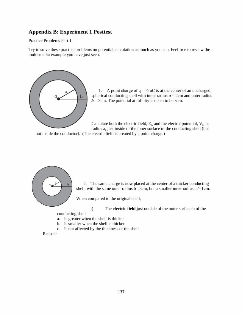
137
Appendix B: Experiment 1 Posttest
Practice Problems Part 1.
Try to solve these practice problems on potential calculation as much as you can. Feel free to review the
multi-media example you have just seen.
1. A point charge of q = 6 μC is at the center of an uncharged
spherical conducting shell with inner radius a = 2cm and outer radius
b = 3cm. The potential at infinity is taken to be zero.
Calculate both the electric field, Ea, and the electric potential, Va, at
radius a, just inside of the inner surface of the conducting shell (but
not inside the conductor). (The electric field is created by a point charge.)
2. The same charge is now placed at the center of a thicker conducting
shell, with the same outer radius b= 3cm, but a smaller inner radius, a’=1cm.
When compared to the original shell,
i) The electric field just outside of the outer surface b of the
conducting shell
a. Is greater when the shell is thicker
b. Is smaller when the shell is thicker
c. Is not affected by the thickness of the shell
Reason:

138
ii) The electric field just inside of the inner surface of the conducting shell
1) Is greater when a’=1cm (thicker shell) than when a=2cm (thinner shell).
2) Is smaller when a’=1cm (thicker shell) than when a=2cm (thinner shell).
3) Is the same in both shells
Reason:
3. The electric potential at the inner surface of the conducting shell
1) Is higher when a’=1cm (thicker shell) than when a=2cm (thinner shell).
2) Is lower when a’=1cm (thicker shell) than when a=2cm (thinner shell).
3) Is the same in both shells
Reason:
4. A conducting sphere of radius a carries positive charge Q. If the potential at
infinity is defined to be zero,
Which of the following graphs represents the electric potential in space as a function of r?
(a) (b) (c) (d)

139
5. A positive point charge Q is placed in space. Point A is located
at a distance Ra away from the charge, and point B is located at Rb away
from the charge.
An uncharged spherical conducting shell is now placed around the
charge. Point A is enclosed in the shell, and point B is outside of the
shell.
After placing the shell, how does the electric field at point B change?
(Hint: Create a Gaussian surface with radius Rb. Does the total charge
inside the surface change after placing the shell?)
a. Stays the same
b. Increases
c. Decreases
d. There will be no E-field at point B.
Reason:
6. After placing the shell, the potential difference between points A and B:
i. Stays the same
ii. Increases
iii. Decreases
iv. Goes to zero
Reason:

140
7. Calculate the potential difference Va-Vb , after the conducting shell is placed. Please explicitly
show how you would set up the integral(s) ; specify the limits of your integral(s), and express
electric fields in terms of k,Q, and r.
8. The conducting shell is now made bigger by increasing
Rin and Rout at the same time. The thickness of the shell, (Rout-
Rin), is unchanged. Point B is still on the outside of the shell.
Will this bigger conducting shell change the value of Va-Vb? If
so, will it become bigger or smaller?

141
Now please click on the second slide in the multimedia tutorial, which will give
you a detailed explanation on the solution of the last two problems you just
did.
Please do NOT change your previous answers after viewing the multimedia.

142
1. For the charge and shell in the previous problems,
which of the following graphs correctly represent the electric potential in
space?
2. What will happen to the potential
difference between A and B, if the inner radius of the shell stays the
same and the outer radius increases, i.e. the shell becomes thicker?
Why?
(a) (b)
(c) (d)

143
3. A point charge Q is surrounded by an
infinitely thin spherical insulating shell with radius R1. The shell
is charged with positive charge +q.
Point A is located at distance RA away from the charge,
and point B is located at distance RB away from the charge.
First, reason why the electric field at point B now becomes k( ) ,
but the electric field at point A remains to be kQ/Ra2.(Hint: set up two
Gaussian surfaces with radius RB and RA respectively, and find the total
charge enclosed inside each surface.)
4. Calculate the potential difference between points A and B. Explicitly write down the
each step of calculation.

144
5. If the radius of the shell becomes smaller,
i.e. the shell is closer to point A and further away from point B,
how would the electric field at points A and B change? (Hint: does
the charges enclosed inside your Gaussian surfaces change?)
6. If the radius of the shell becomes smaller, how would the potential difference
between A and B change? Why?

145
Appendix C: Experiment 1 Posttest Detailed Grading from each grader
Percentage of correct (=3) answer for each problem in Experiment 1.
Grader 1 (%) P1-1 P1-3 P1-4 P1-6&7 P1-8
Crtl 0.21 0.21 0.26 0.21 0.05
Exp 0.55 0.45 0.30 0.60 0.15
CInf 0.25 0.25 0.25 0.50 0.06
Grader 2 P1-1 P1-3 P1-4 P1-6&7 P1-8
Crtl 0.17 0.17 0.28 0.28 0.11
Exp 0.55 0.45 0.30 0.70 0.15
CInf 0.19 0.25 0.25 0.50 0.13
Part 2
Grader 1 P2-1 P2-2 P2-4 P2-6
Crtl 0.00 0.83 0.50 0.11
Exp 0.45 0.85 0.60 0.50
CInf 0.13 0.69 0.56 0.13
Grader 2 P2-1 P2-2 P2-4 P2-6
Crtl 0.00 0.67 0.39 0.06
Exp 0.45 0.90 0.50 0.45
CInf 0.13 0.56 0.50 0.19
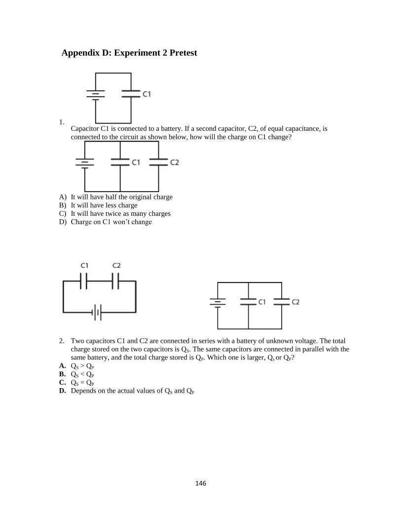
146
Appendix D: Experiment 2 Pretest
1. Capacitor C1 is connected to a battery. If a second capacitor, C2, of equal capacitance, is
connected to the circuit as shown below, how will the charge on C1 change?
A) It will have half the original charge
B) It will have less charge
C) It will have twice as many charges
D) Charge on C1 won’t change
2. Two capacitors C1 and C2 are connected in series with a battery of unknown voltage. The total
charge stored on the two capacitors is QS. The same capacitors are connected in parallel with the
same battery, and the total charge stored is QP. Which one is larger, Qs or QP?
A. QS > QP
B. QS < QP
C. QS = QP
D. Depends on the actual values of QS and QP

147
3. Three capacitors of equal capacitance 1μF are connected to a battery of unknown voltage. The
voltage difference between points A and B is measured to be 5V.
1) What is the equivalent capacitance of C1 and C2?
2) What is the charge on capacitor C1?
3) What is the battery voltage?

148
Appendix E: Experiment 2 Posttest Practice problems part 1:
P1-1
Identical capacitors C1 and C2 are connected to a battery as shown.
A third capacitor, C3, of unknown capacitance, is added to the circuit through two different types
of connections, as shown below:
(A) (B)
1) After C3 has been added, in which connection will C2 have a larger voltage difference, V2?
a. In connection A
b. In connection B
c. Both are the same.
d. Depend on the capacitance of C3
2) Compared to the original circuit, how will V1, the voltage difference across capacitor C1,
change in connections A and B? Explain.

149
P1-2. Two capacitors of UNEQUAL capacitance were initially connected in series with a battery, as
shown in figure (1) below. As a result, they have different voltage drops across them.
The switch is then turned to position B for a long time (figure 2), and then turned to position C.
After the switch has turned to position C, in which direction will the current, i.e. positive charges,
move?
(1) (2) (3)
A. Current will flow from C2 to C1 (counter clockwise) since positive charges will
move from higher potential to lower potential.
B. Current will flow from C1 to C2 (clockwise) since positive charges move from
higher potential to lower potential.
C. The charges will not move since there will be no voltage left on the capacitors after
the battery has been removed.
D. The charges will not move since the capacitors are connected in series and they originally have equal
charges.
E. None of the above is the right answer (specify) :

150
P1-3
Capacitors C1, C2 , C3 and C4 are connected to a battery of unknown voltage, as shown. Capacitance of
C1, C2 and C4 are 1 μF, and capacitance of C3 is 3 μF. The voltage difference between points A and B,
VAB = 4V, and the voltage difference between A and C, VAC =5V.
1) What is the voltage difference and charge on capacitor C2?
2) What is the charge stored on capacitor C4?
3) What is the battery voltage?
C1 = 1 μF,
C2 = 1 μF,
C3 = 3 μF,
C4 = 1 μF,
VAB = 4V,
VAC = 5V,

151
P1-4.
Capacitors C1 and C2 are connected in series with a battery. The capacitance of C2 is now increased.
1) How will the charge stored on capacitor C1 change? Explain
2) How will the voltage difference on capacitor C2 change? Explain
Try your best to answer the questions above. When you are done, go ahead and
view slide 3 of the animated tutorial.
Please do NOT change any of your previous answers once you have viewed slide 3.
152
Part 2
P2-1 A B
Capacitors C1 and C2 are connected with two different batteries in two different ways, as shown above.
Initially, the batteries were chosen so that the charge Q2 stored on capacitor C2 are the same in circuits A
and B.
The capacitance of C2 is then increased to twice its initial value.
1) As a result, the charge stored on the capacitor will:
A) Increase in circuit A and decrease in circuit B
B) Decrease in circuit A and increase in circuit B
C) Increase in both circuits.
D) Decrease in both circuits.
E) They will not change
2) After C2 has doubled, will Q2 still be the same in both circuits? If not, in which circuit will Q2 be
larger? Why?

153
P2-2
Three capacitors of equal capacitance, C1, C2 and C3, are connected to a battery as shown. The
capacitance of C2 is now increased.
1) How will the voltage difference across capacitor C1 change? Why?
2) How will the charge on capacitor C3 change? Why?
3) How will the total charge on capacitors C2 and C3 change? Why?
(This is the end of the review session.)