Prepared for submission to JHEP ARC-17-5

Surface operators, chiral rings and localization in

N = 2 gauge theories

S. K. Ashok,a,b M. Billo,c,d E. Dell’Aquila,c M. Frau,c,d V. Gupta,a,b R. R. John,a,b and

A. Lerda e,d

aInstitute of Mathematical Sciences

C. I. T. Campus, Taramani

Chennai, India 600113

bHomi Bhabha National Institute

Training School Complex, Anushakti Nagar,

Mumbai, India 400085

cUniversita di Torino, Dipartimento di FisicadArnold-Regge Center and I. N. F. N. - sezione di Torino,

Via P. Giuria 1, I-10125 Torino, Italy

eUniversita del Piemonte Orientale, Dipartimento di Scienze e Innovazione Tecnologica

Viale T. Michel 11, I-15121 Alessandria, Italy

E-mail: sashok@imsc.res.in, billo@to.infn.it, edellaquila@gmail.com,

frau@to.infn.it, varungupta@imsc.res.in, renjan@imsc.res.in,

lerda@to.infn.it

Abstract: We study half-BPS surface operators in supersymmetric gauge theories in four

and five dimensions following two different approaches. In the first approach we analyze

the chiral ring equations for certain quiver theories in two and three dimensions, coupled

respectively to four- and five-dimensional gauge theories. The chiral ring equations, which

arise from extremizing a twisted chiral superpotential, are solved as power series in the

infrared scales of the quiver theories. In the second approach we use equivariant localization

and obtain the twisted chiral superpotential as a function of the Coulomb moduli of the

four- and five-dimensional gauge theories, and find a perfect match with the results obtained

from the chiral ring equations. In the five-dimensional case this match is achieved after

solving a number of subtleties in the localization formulas which amounts to choosing

a particular residue prescription in the integrals that yield the Nekrasov-like partition

functions for ramified instantons. We also comment on the necessity of including Chern-

Simons terms in order to match the superpotentials obtained from dual quiver descriptions

of a given surface operator.

Keywords: N = 2 gauge theories, instantons, surface operators

arX

iv:1

707.

0892

2v3

[he

p-th

] 2

2 D

ec 2

017

Contents

1 Introduction 1

2 Twisted superpotential for coupled 2d/4d theories 3

2.1 SU(2) 4

2.2 Twisted chiral ring in quiver gauge theories 7

2.3 SU(3) 12

3 Twisted superpotential for coupled 3d/5d theories 14

3.1 Twisted chiral ring in quiver gauge theories 15

3.2 SU(2) and SU(3) 19

4 Ramified instantons in 4d and 5d 21

4.1 Localization in 4d 21

4.2 Localization in 5d 26

5 Superpotentials for dual quivers 28

5.1 Adding Chern-Simons terms 31

6 Conclusions and perspectives 33

A Chiral correlators in 5d 34

B Chern-Simons terms in an SU(4) example 35

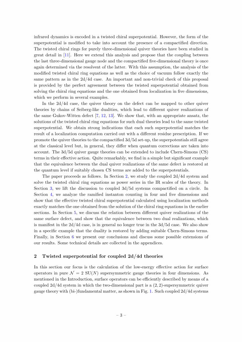
1 Introduction

In this paper we study the low-energy effective action that governs the dynamics of half-BPS

surface operators in theories with eight supercharges. We focus on pure SU(N) theories in

four dimensions and in five dimensions compactified on a circle, and explore their Coulomb

branch where the adjoint scalars acquire a vacuum expectation value (vev).

In four dimensions, a surface defect supports on its world-volume a two-dimensional

gauge theory that is coupled to the “bulk” four-dimensional theory, see [1] for a review.

This combined 2d/4d system is described by two holomorphic functions: the prepotential

F and the twisted superpotential W . The prepotential governs the dynamics of the bulk

theory and depends on the Coulomb vev’s and the infra-red (IR) scale of the gauge theory

in four dimensions. The twisted superpotential controls the two-dimensional dynamics on

the surface operator, and is a function of the continuous parameters labeling the defect,

the two-dimensional IR scales, and also of the Coulomb vev’s and the strong-coupling scale

– 1 –

of the bulk gauge theory. The twisted superpotential thus describes the coupled 2d/4d

system.

Surface operators in theories with eight supercharges can be studied from diverse points

of view. One approach is to treat them as monodromy defects (also known as Gukov-Witten

defects) in four dimensions along the lines discussed in [2, 3] and compute the corresponding

twisted superpotential W using equivariant localization as shown for example in [4–7]. A

second approach is to focus on the two-dimensional world-volume theory on the surface

operator [8]. In the superconformal theories of class S, a microscopic description of a generic

co-dimension 4 surface operator in terms of (2, 2) supersymmetric quiver gauge theories

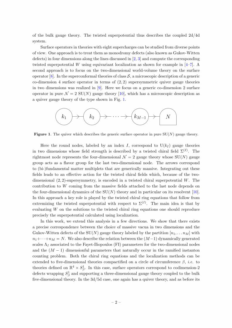
in two dimensions was realized in [9]. Here we focus on a generic co-dimension 2 surface

operator in pure N = 2 SU(N) gauge theory [10], which has a microscopic description as

a quiver gauge theory of the type shown in Fig. 1.

k1 k2. . . kM−1 N

Figure 1. The quiver which describes the generic surface operator in pure SU(N) gauge theory.

Here the round nodes, labeled by an index I, correspond to U(kI) gauge theories

in two dimensions whose field strength is described by a twisted chiral field Σ(I). The

rightmost node represents the four-dimensional N = 2 gauge theory whose SU(N) gauge

group acts as a flavor group for the last two-dimensional node. The arrows correspond

to (bi-)fundamental matter multiplets that are generically massive. Integrating out these

fields leads to an effective action for the twisted chiral fields which, because of the two-

dimensional (2, 2)-supersymmetry, is encoded in a twisted chiral superpotential W . The

contribution to W coming from the massive fields attached to the last node depends on

the four-dimensional dynamics of the SU(N) theory and in particular on its resolvent [10].

In this approach a key role is played by the twisted chiral ring equations that follow from

extremizing the twisted superpotential with respect to Σ(I). The main idea is that by

evaluating W on the solutions to the twisted chiral ring equations one should reproduce

precisely the superpotential calculated using localization.

In this work, we extend this analysis in a few directions. We show that there exists

a precise correspondence between the choice of massive vacua in two dimensions and the

Gukov-Witten defects of the SU(N) gauge theory labeled by the partition [n1, . . . nM ] with

n1+· · ·+nM = N . We also describe the relation between the (M−1) dynamically generated

scales ΛI associated to the Fayet-Iliopoulos (FI) parameters for the two-dimensional nodes

and the (M − 1) dimensionful parameters that naturally occur in the ramified instanton

counting problem. Both the chiral ring equations and the localization methods can be

extended to five-dimensional theories compactified on a circle of circumference β, i.e. to

theories defined on R4 × S1β. In this case, surface operators correspond to codimension-2

defects wrapping S1β and supporting a three-dimensional gauge theory coupled to the bulk

five-dimensional theory. In the 3d/5d case, one again has a quiver theory, and as before its

– 2 –

infrared dynamics is encoded in a twisted chiral superpotential. However, the form of the

superpotential is modified to take into account the presence of a compactified direction.

The twisted chiral rings for purely three-dimensional quiver theories have been studied in

great detail in [11]. Here we extend this analysis and propose that the coupling between

the last three-dimensional gauge node and the compactified five-dimensional theory is once

again determined via the resolvent of the latter. With this assumption, the analysis of the

modified twisted chiral ring equations as well as the choice of vacuum follow exactly the

same pattern as in the 2d/4d case. An important and non-trivial check of this proposal

is provided by the perfect agreement between the twisted superpotential obtained from

solving the chiral ring equations and the one obtained from localization in five dimensions,

which we perform in several examples.

In the 2d/4d case, the quiver theory on the defect can be mapped to other quiver

theories by chains of Seiberg-like dualities, which lead to different quiver realizations of

the same Gukov-Witten defect [7, 12, 13]. We show that, with an appropriate ansatz, the

solutions of the twisted chiral ring equations for such dual theories lead to the same twisted

superpotential. We obtain strong indications that each such superpotential matches the

result of a localization computation carried out with a different residue prescription. If we

promote the quiver theories to the compactified 3d/5d set-up, the superpotentials still agree

at the classical level but, in general, they differ when quantum corrections are taken into

account. The 3d/5d quiver gauge theories can be extended to include Chern-Simons (CS)

terms in their effective action. Quite remarkably, we find in a simple but significant example

that the equivalence between the dual quiver realizations of the same defect is restored at

the quantum level if suitably chosen CS terms are added to the superpotentials.

The paper proceeds as follows. In Section 2, we study the coupled 2d/4d system and

solve the twisted chiral ring equations as power series in the IR scales of the theory. In

Section 3, we lift the discussion to coupled 3d/5d systems compactified on a circle. In

Section 4, we analyze the ramified instanton counting in four and five dimensions and

show that the effective twisted chiral superpotential calculated using localization methods

exactly matches the one obtained from the solution of the chiral ring equations in the earlier

sections. In Section 5, we discuss the relation between different quiver realizations of the

same surface defect, and show that the equivalence between two dual realizations, which

is manifest in the 2d/4d case, is in general no longer true in the 3d/5d case. We also show

in a specific example that the duality is restored by adding suitable Chern-Simons terms.

Finally, in Section 6 we present our conclusions and discuss some possible extensions of

our results. Some technical details are collected in the appendices.

2 Twisted superpotential for coupled 2d/4d theories

In this section our focus is the calculation of the low-energy effective action for surface

operators in pure N = 2 SU(N) supersymmetric gauge theories in four dimensions. As

mentioned in the Introduction, surface operators can be efficiently described by means of a

coupled 2d/4d system in which the two-dimensional part is a (2, 2)-supersymmetric quiver

gauge theory with (bi-)fundamental matter, as shown in Fig. 1. Such coupled 2d/4d systems

– 3 –

have an alternative description as Gukov-Witten monodromy defects [2, 3]. The discrete

data that label these defects correspond to the partitions of N , and can be summarized in

the notation SU(N)[n1, . . . , nM ] where n1 + · · ·+ nM = N . The M integers nI are related

to the breaking pattern (or Levi decomposition) of the four-dimensional gauge group on

the defect, namely

SU(N) −→ S[U(n1)× . . .×U(nM )

]. (2.1)

They also determine the ranks kI of the two-dimensional gauge groups of the quiver in

Fig. 1 according to

kI = n1 + · · ·+ nI . (2.2)

The (bi-)fundamental fields connecting two nodes turn out to be massive. Integrating

them out leads to the low-energy effective action for the gauge multiplet. In the I-th node

the gauge multiplet is described by a twisted chiral field Σ(I) and the low-energy effective

action is encoded in a twisted chiral superpotential W (Σ(I)). The vacuum structure can

be determined by the twisted chiral ring equations, which take the form [14–16]

exp( ∂W

∂Σ(I)s

)= 1 (2.3)

where Σ(I)s are the diagonal components, with s = 1, . . . , k [17]. This exponentiated form

of the equations is a consequence of the electric fluxes which can be added to minimize the

potential energy and which lead to linear (in Σ(I)) terms in the effective superpotential.

We extend this analysis in the following manner: first of all, we show that in the

classical limit there is a very specific choice of solutions to the twisted chiral ring equations

that allows us to make contact with the twisted chiral superpotential calculated using

localization. We establish the correspondence between the continuous parameters labeling

the monodromy defect and the dynamically generated scales of the two-dimensional quiver

theory. We then show that quantum corrections in the quiver gauge theory are mapped

directly to corrections in the twisted superpotential due to ramified instantons of the four-

dimensional theory.

2.1 SU(2)

As an illustrative example, we consider the simple surface operator in the pure SU(2)

theory which is represented by the partition [1, 1]. From the two-dimensional perspective,

the effective dynamics is described by a non-linear sigma model with target-space CP1,

coupled to the four-dimensional SU(2) gauge theory in a particular way that we now

describe. We use the gauged linear sigma model (GLSM) description of this theory [17, 18]

in order to study its vacuum structure. We essentially follow the discussion in [10] although,

as we shall see in detail, there are some differences in our analysis. The GLSM is a U(1)

gauge theory with two chiral multiplets in the fundamental representation, that can be

associated to the quiver drawn in Fig. 2.

Let us first analyze the simple case in which the quantum effects of the SU(2) theory

are neglected. We consider a generic point in the Coulomb branch parameterized by the

vev’s a1 = −a2 = a of the adjoint SU(2) scalar field Φ in the vector multiplet. These

– 4 –

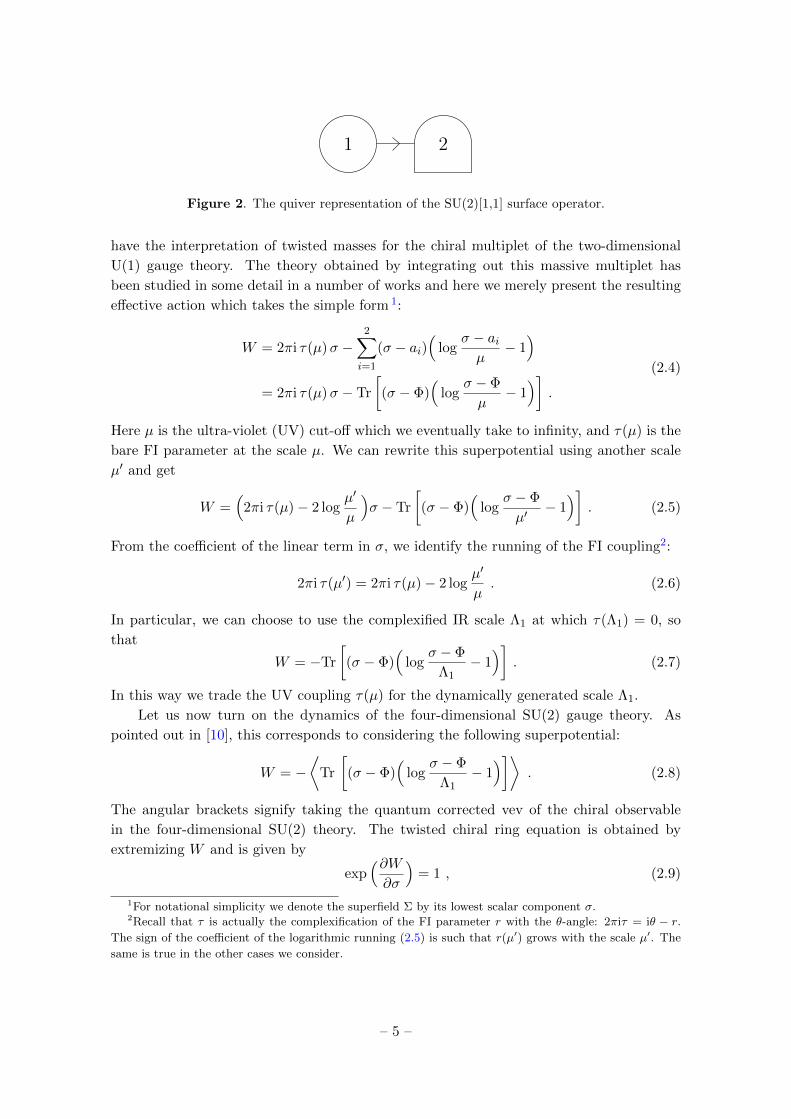
1 2

Figure 2. The quiver representation of the SU(2)[1,1] surface operator.

have the interpretation of twisted masses for the chiral multiplet of the two-dimensional

U(1) gauge theory. The theory obtained by integrating out this massive multiplet has

been studied in some detail in a number of works and here we merely present the resulting

effective action which takes the simple form 1:

W = 2πi τ(µ)σ −2∑i=1

(σ − ai)(

logσ − aiµ− 1)

= 2πi τ(µ)σ − Tr

[(σ − Φ)

(log

σ − Φ

µ− 1)]

.

(2.4)

Here µ is the ultra-violet (UV) cut-off which we eventually take to infinity, and τ(µ) is the

bare FI parameter at the scale µ. We can rewrite this superpotential using another scale

µ′ and get

W =(

2πi τ(µ)− 2 logµ′

µ

)σ − Tr

[(σ − Φ)

(log

σ − Φ

µ′− 1)]

. (2.5)

From the coefficient of the linear term in σ, we identify the running of the FI coupling2:

2πi τ(µ′) = 2πi τ(µ)− 2 logµ′

µ. (2.6)

In particular, we can choose to use the complexified IR scale Λ1 at which τ(Λ1) = 0, so

that

W = −Tr

[(σ − Φ)

(log

σ − Φ

Λ1− 1)]

. (2.7)

In this way we trade the UV coupling τ(µ) for the dynamically generated scale Λ1.

Let us now turn on the dynamics of the four-dimensional SU(2) gauge theory. As

pointed out in [10], this corresponds to considering the following superpotential:

W = −⟨

Tr

[(σ − Φ)

(log

σ − Φ

Λ1− 1)]⟩

. (2.8)

The angular brackets signify taking the quantum corrected vev of the chiral observable

in the four-dimensional SU(2) theory. The twisted chiral ring equation is obtained by

extremizing W and is given by

exp(∂W∂σ

)= 1 , (2.9)

1For notational simplicity we denote the superfield Σ by its lowest scalar component σ.2Recall that τ is actually the complexification of the FI parameter r with the θ-angle: 2πiτ = iθ − r.

The sign of the coefficient of the logarithmic running (2.5) is such that r(µ′) grows with the scale µ′. The

same is true in the other cases we consider.

– 5 –

which, using the superpotential (2.8), is equivalent to

exp

⟨Tr log

σ − Φ

Λ1

⟩= 1 . (2.10)

As explained in [10], the left-hand side of (2.10) is simply the integral of the resolvent of

the pure N = 2 SU(2) theory in four dimensions which takes the form [19]:⟨Tr log

σ − Φ

Λ1

⟩= log

(P2(σ) +

√P2(σ)2 − 4Λ4

2Λ21

). (2.11)

Here Λ is the four-dimensional strong coupling scale of the SU(2) theory and

P2(σ) = σ2 − u (2.12)

is the characteristic polynomial appearing in the Seiberg-Witten solution where

u =1

2

⟨Tr Φ2

⟩= a2 +

Λ4

2a2+

5Λ8

32a6+ . . . (2.13)

Using (2.11) and performing some simple manipulations, we find that the twisted chiral

ring relation (2.10) becomes

P2(σ) = Λ21 +

Λ4

Λ21

(2.14)

from which we obtain the two solutions

σ±? (u,Λ1) = ±

√u+ Λ2

1 +Λ4

Λ21

. (2.15)

Notice the explicit presence of two different scales, Λ1 and Λ, which are related respec-

tively to the two-dimensional and the four-dimensional dynamics. Clearly, the purely

two-dimensional result can be recovered by taking the Λ→ 0 limit. We can now substitute

either one of the solutions of the chiral ring equation into the twisted chiral superpotential

and obtain a function W±? . The proposal in [10] is that this should reproduce the twisted

superpotential calculated using localization methods. We shall explicitly verify this in Sec-

tion 4, but here we would like to point out an important simplification that occurs in this

calculation.

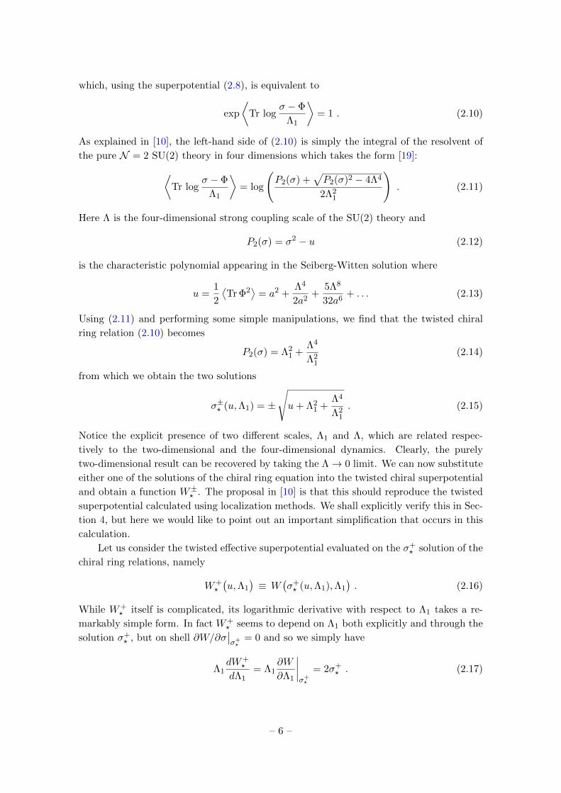
Let us consider the twisted effective superpotential evaluated on the σ+? solution of the

chiral ring relations, namely

W+?

(u,Λ1

)≡ W

(σ+? (u,Λ1),Λ1

). (2.16)

While W+? itself is complicated, its logarithmic derivative with respect to Λ1 takes a re-

markably simple form. In fact W+? seems to depend on Λ1 both explicitly and through the

solution σ+? , but on shell ∂W/∂σ

∣∣σ+?

= 0 and so we simply have

Λ1dW+

?

dΛ1= Λ1

∂W

∂Λ1

∣∣∣∣σ+?

= 2σ+? . (2.17)

– 6 –

where in the last step we used (2.8) and took into account the tracelessness of Φ.

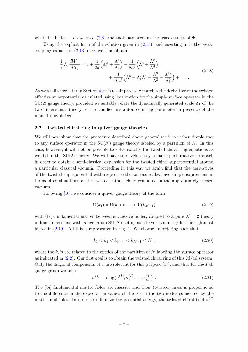
Using the explicit form of the solution given in (2.15), and inserting in it the weak-

coupling expansion (2.13) of u, we thus obtain

1

2Λ1dW+

?

dΛ1= a+

1

2a

(Λ2

1 +Λ4

Λ21

)− 1

8a3

(Λ4

1 +Λ8

Λ41

)+

1

16a5

(Λ6

1 + Λ21Λ4 +

Λ8

Λ21

+Λ12

Λ61

)+ . . . .

(2.18)

As we shall show later in Section 4, this result precisely matches the derivative of the twisted

effective superpotential calculated using localization for the simple surface operator in the

SU(2) gauge theory, provided we suitably relate the dynamically generated scale Λ1 of the

two-dimensional theory to the ramified instanton counting parameter in presence of the

monodromy defect.

2.2 Twisted chiral ring in quiver gauge theories

We will now show that the procedure described above generalizes in a rather simple way

to any surface operator in the SU(N) gauge theory labeled by a partition of N . In this

case, however, it will not be possible to solve exactly the twisted chiral ring equations as

we did in the SU(2) theory. We will have to develop a systematic perturbative approach

in order to obtain a semi-classical expansion for the twisted chiral superpotential around

a particular classical vacuum. Proceeding in this way we again find that the derivatives

of the twisted superpotential with respect to the various scales have simple expressions in

terms of combinations of the twisted chiral field σ evaluated in the appropriately chosen

vacuum.

Following [10], we consider a quiver gauge theory of the form

U(k1)×U(k2)× . . .×U(kM−1) (2.19)

with (bi)-fundamental matter between successive nodes, coupled to a pure N = 2 theory

in four dimensions with gauge group SU(N) acting as a flavor symmetry for the rightmost

factor in (2.19). All this is represented in Fig. 1. We choose an ordering such that

k1 < k2 < k3 . . . < kM−1 < N , (2.20)

where the kI ’s are related to the entries of the partition of N labeling the surface operator

as indicated in (2.2). Our first goal is to obtain the twisted chiral ring of this 2d/4d system.

Only the diagonal components of σ are relevant for this purpose [17], and thus for the I-th

gauge group we take

σ(I) = diag(σ

(I)1 , σ

(I)2 , . . . , σ

(I)kI

). (2.21)

The (bi)-fundamental matter fields are massive and their (twisted) mass is proportional

to the difference in the expectation values of the σ’s in the two nodes connected by the

matter multiplet. In order to minimize the potential energy, the twisted chiral field σ(I)

– 7 –

gets a vev and this in turn leads to a non-vanishing mass for the (bi)-fundamental matter.

Integrating out these massive fields, we obtain the following effective superpotential

W = 2πi

M−1∑I=1

kI∑s=1

τI(µ)σ(I)s −

M−2∑I=1

kI∑s=1

kI+1∑t=1

$(σ(I)s − σ

(I+1)t

)−kM−1∑s=1

⟨Tr$

(σ(M−1)s − Φ

)⟩ (2.22)

where, for compactness, we have introduced the function

$(x) = x(

logx

µ− 1)

(2.23)

with µ being the UV cut-off scale. Similarly to the SU(2) example previously considered,

also here we can trade the UV parameters τI(µ) for the dynamically generated scales ΛI for

each of the gauge groups in the quiver. To this aim, we unpackage of the terms containing

the $-function and rewrite them as follows:

$(σ(I)s − σ

(I+1)t

)=σ(I)

s

(log

σ(I)s − σ(I+1)

t

ΛI− 1

)− σ(I+1)

t

(log

σ(I)s − σ(I+1)

t

ΛI+1− 1

)+ σ(I)

s logΛIµ− σ(I+1)

t logΛI+1

µ

(2.24)

for I = 1, . . . ,M − 2, and

Tr$(σ(M−1)s − Φ

)= Tr

[(σ(M−1)s − Φ)

(log

σ(M−1)s − Φ

ΛM−1− 1

)]

+N σ(M−1)s log

ΛM−1

µ.

(2.25)

Considering the linear terms in the σ(I) fields we see that the FI couplings change with the

scale and we can define the dynamically generated scales ΛI to be such that

τI(ΛI) = τI(µ)− kI+1 − kI−1

2πilog

ΛIµ

= 0 (2.26)

for I = 1, . . . ,M − 1 3. Equivalently, we can write

ΛbII = e2πi τI(µ) µbI (2.27)

where

bI = kI+1 − kI−1 (2.28)

denotes the coefficient of the β-function for the running of the FI parameter of the I-th

node.

3We assume that k0 = 0 and kM = N .

– 8 –

Using these expressions, the twisted superpotential (2.22) can thus be rewritten as

W =−M−2∑I=1

kI∑s=1

kI+1∑t=1

σ(I)s

(log

σ(I)s − σ(I+1)

t

ΛI− 1

)

+M−1∑I=2

kI∑s=1

kI−1∑r=1

σ(I)s

(log

σ(I−1)r − σ(I)

s

ΛI− 1

)

−kM−1∑s=1

⟨Tr

[(σ(M−1)s − Φ)

(log

σ(M−1)s − Φ

ΛM−1− 1

)]⟩.

(2.29)

The I-th term (1 ≤ I ≤ M − 2)) in the first line and the (I + 1)-th term in the second

line of this expression are obtained by integrating out the bifundamental fields between the

nodes I and I + 1, while the last line is the result of integrating out the fundamental fields

attached to the last gauge node of the quiver. The angular brackets account for the four-

dimensional dynamics of the SU(N) theory. One can easily verify that for N = M = 2,

the expression in (2.29) reduces to (2.8).

The twisted chiral ring

The twisted chiral ring relations are given by

exp( ∂W∂σ

(I)s

)= 1 . (2.30)

In order to write the resulting equations in a compact form, we define a characteristic

gauge polynomial for each of the SU(kI) node of the quiver

QI(z) =

kI∏s=1

(z − σ(I)s ) . (2.31)

For I = 1, . . . ,M − 2, the equations are independent of the four-dimensional theory, and

read

QI+1(z) = (−1)kI−1 ΛbII QI−1(z) (2.32)

with z = σ(I)s for each s, and with the understanding that Q0 = 1 and k0 = 0. Note

that the power of ΛI , which is determined by the running of the FI coupling, makes the

equation consistent from a dimensional point of view. For I = M − 1, the presence of the

four-dimensional SU(N) gauge theory affects the last two-dimensional node of the quiver,

and the corresponding chiral ring equation is

exp⟨

Tr logz − Φ

ΛM−1

⟩= (−1)kM−2 Λ

bM−1−NM−1 QM−2(z) (2.33)

with z = σ(M−1)s for each s. We now use the fact that the resolvent of the four-dimensional

SU(N) theory, which captures all information about the chiral correlators, is given by [19]

T (z) :=

⟨Tr

1

z − Φ

⟩=

P ′N (z)√PN (z)2 − 4Λ2N

(2.34)

– 9 –

where PN (z) is the characteristic polynomial of degree N encoding the Coulomb vev’s of the

SU(N) theory and Λ is its dynamically generated scale. Since we are primarily interested

in the semi-classical solution of the chiral ring equations, we exploit the fact that PN (z)

can be written as a perturbation of the classical gauge polynomial in the following way:

PN (z) =

N∏i=1

(z − ei) (2.35)

where ei are the quantum vev’s of the pure SU(N) theory given by [20, 21]

ei = ai − Λ2N ∂

∂ai

(∏j 6=i

1

a2ij

)+O(Λ4N ) . (2.36)

Integrating the resolvent (2.34) with respect to z and exponentiating the resulting expres-

sion, one finds

exp⟨

Tr logz − Φ

ΛM−1

⟩=

PN (z) +√PN (z)2 − 4Λ2N

2ΛNM−1

. (2.37)

Using this, we can rewrite the twisted chiral ring relation (2.33) associated to the last node

of the quiver in the following form:

PN (z) +√PN (z)2 − 4Λ2N = 2 (−1)kM−2 Λ

bM−1

M−1 QM−2(z) , (2.38)

where z = σ(M−1)s . With further simple manipulations, we obtain

PN (z) = (−1)kM−2 ΛbM−1

M−1 QM−2(z) +Λ2N

(−1)kM−2 ΛbM−1

M−1 QM−2(z)(2.39)

for z = σ(M−1)s . In the limit Λ→ 0 which corresponds to turning off the four-dimensional

dynamics, we obtain the expected twisted chiral ring relation of the last two-dimensional

node of the quiver. Equations (2.32) and (2.39) are the relevant chiral relations which we

are going to solve order by order in the ΛI ’s to obtain the weak-coupling expansion of the

twisted chiral superpotential.

Solving the chiral ring equations

Our goal is to provide a systematic procedure to solve the twisted chiral ring equations

we have just derived and to find the effective twisted superpotential of the 2d/4d theory.

As illustrated in the case of the SU(2) theory in Section 2.1, we shall do so by evaluating

W on the solutions of the twisted chiral ring equations. Each choice of vacuum therefore

corresponds to a different surface operator.

In order to clarify this last point, we first solve the classical chiral ring equations, which

are obtained by setting ΛI and Λ to zero keeping their ratio fixed, i.e. by considering the

– 10 –

theory at a scale much bigger than ΛI and Λ. Thus, in this limit the right-hand sides of

(2.32) and (2.39) vanish. A possible choice 4 that accomplishes this is:

σ(1)s = as for s = 1, . . . , k1 ,

σ(2)t = at for t = 1, . . . , k2 ,

...

σ(M−1)w = aw for w = 1, . . . , kM−1 .

(2.40)

This is equivalent to assuming that the classical expectation value of σ for the I-th node is

σ(I) = diag(a1, a2, . . . , akI

). (2.41)

We will see that this choice is the one appropriate to describe a surface defect that breaks

the gauge group SU(N) according to the Levi decomposition (2.1).

Let us now turn to the quantum chiral ring equations. Here we make an ansatz for

σ(I) as a power series in the various ΛI ’s around the chosen classical vacuum. From the

explicit expressions (2.32) and (2.39) of the chiral ring equations, it is easy to realize that

there is a natural set of parameters in terms of which these power series can be written;

they are given by

qI = (−1)kI−1 ΛbII (2.42)

for I = 1, . . . ,M − 1. If the four-dimensional theory were not dynamical, these (M − 1)

parameters would be sufficient; however, from the chiral ring equations (2.39) of the last

two-dimensional node of the quiver, we see that another parameter is needed. It is related

to the four-dimensional scale Λ and hence to the four-dimensional instanton action. It

turns out that this remaining expansion parameter is

qM = (−1)N Λ2N(M−1∏I=1

qI

)−1. (2.43)

Our proposal is to solve the chiral ring equations (2.32) and (2.39) as a simultaneous power

series in all the qI ’s, including qM , which ultimately will be identified with the Nekrasov-like

counting parameters in the ramified instanton computations described in Section 4.

We will explicitly illustrate these ideas in some examples in the next section, but first

we would like to show in full generality that the logarithmic derivatives with respect to

ΛI are directly related to the solution σ(I)? of the twisted chiral ring equations (2.32) and

(2.39). The argument is a straightforward generalization of what we have already seen in

the SU(2) case, see (2.16) and (2.17). On shell, i.e. when ∂W/∂σ∣∣σ?

= 0, the twisted

superpotential W? ≡ W (σ?) depends on ΛI only explicitly. Using the expression of W

given in (2.29), we find

ΛIdW?

dΛI= ΛI

∂W

∂ΛI

∣∣∣∣σ?

= bI trσ(I)? , (2.44)

4All other solutions are related to this one by permuting the a’s.

– 11 –

where in the last step we used the tracelessness of Φ. This relation can be written in terms

of the parameters qI defined in (2.42), as follows

qIdW?

dqI= trσ

(I)? . (2.45)

If we express the solution σ? of the chiral ring equations as the classical solution (2.40)

plus quantum corrections, we find

q1dW?

dq1= a1 + . . . ak1 + corr.ns = a1 + . . .+ an1 + corr.ns ,

q2dW?

dq2= a1 + . . . ak2 + corr.ns = a1 + . . .+ an1+n2 + corr.ns

(2.46)

and so on. This corresponds to a partition of the classical vev’s of the SU(N) theory given

by ︸ ︷︷ ︸

n1

a1, · · · an1 , ︸ ︷︷ ︸n2

an1+1, · · · an1+n2 , · · · , ︸ ︷︷ ︸nM

aN−nM+1, . . . aN

, (2.47)

which is interpreted as a breaking of the gauge group SU(N) according to the Levi de-

composition (2.1). In fact, by comparing with the results of [6] (see for instance, equation

(4.1) of this reference), we see that the expressions (2.46) coincide with the derivatives of

the classical superpotential describing the surface operator of the SU(N) theory, labeled

by the partition [n1, n2, . . . , nM ], provided we relate the parameters qI to the variables tJthat label the monodromy defect according to

2πi tJ ∼M∑I=I

log qI for J = 1, . . . ,M . (2.48)

We now illustrate these general ideas in a few examples.

2.3 SU(3)

We consider the surface operators in the SU(3) theory. There are two distinct partitions,

namely [1, 2] and [1, 1, 1], which we now discuss in detail.

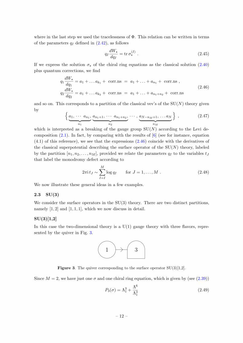
SU(3)[1,2]

In this case the two-dimensional theory is a U(1) gauge theory with three flavors, repre-

sented by the quiver in Fig. 3.

1 3

Figure 3. The quiver corresponding to the surface operator SU(3)[1,2].

Since M = 2, we have just one σ and one chiral ring equation, which is given by (see (2.39))

P3(σ) = Λ31 +

Λ6

Λ31

(2.49)

– 12 –

where the gauge polynomial is defined in (2.35). We solve this equation order by order in

Λ1 and Λ, using the ansatz

σ? = a1 +∑`1,`2

c`1,`2 q`11 q`22 (2.50)

where the expansion parameters are defined in (2.42) and (2.43), which in this case explicitly

read

q1 = Λ31 , q2 = −Λ6

Λ31

. (2.51)

Inserting (2.50) into (2.49), we can recursively determine the coefficients c`1`2 and, at the

first orders, find the following result

σ? = a1 +1

a12 a13

(Λ3

1 +Λ6

Λ31

)−( 1

a312 a

213

+1

a212 a

313

)(Λ6

1 +Λ12

Λ61

)+ . . . (2.52)

where aij = ai − aj . According to (2.45), this solution coincides with the q1-logarithmic

derivative of the twisted superpotential. We will verify this statement by comparing (2.52)

against the result obtained via localization methods.

SU(3)[1,1,1]

In this case the two-dimensional theory is represented by the quiver of Fig. 4.

1 2 3

Figure 4. The quiver diagram representing the surface operator SU(3)[1,1,1].

Since M = 3, there are now two sets of twisted chiral ring equations. For the first node,

from (2.32) we find

2∏s=1

(σ(1) − σ(2)

s

)= Λ2

1 , (2.53)

while for the second node, from (2.39) we get

P3

(σ(2)s

)= −Λ2

2

(σ(2)s − σ(1)

)− Λ6

Λ22

(σ

(2)s − σ(1)

) (2.54)

for s = 1, 2. From the classical solution to these equations (see (2.41)), we realize that this

configuration corresponds to a surface operator specified by the partition of the Coulomb

vev’s a1, a2, a3, which is indeed associated to the partition [1,1,1] we are consid-

ering. Thus, the ansatz for solving the quantum equations (2.53) and (2.54) takes the

– 13 –

following form:

σ(1)? = a1 +

∑`1,`2,`3

d`1,`2,`3 q`11 q`22 q`33 ,

σ(2)?,1 = a1 +

∑`1,`2,`3

f`1,`2,`3 q`11 q`22 q`33 ,

σ(2)?,2 = a2 +

∑`1,`2,`3

g`1,`2,`3 q`11 q`22 q`33 ,

(2.55)

with

q1 = Λ21 , q2 = −Λ2

2 , q3 =Λ6

Λ21Λ2

2

. (2.56)

Solving the coupled equations (2.53) and (2.54) order by order in qI , we find the following

result:

σ(1)? = a1 +

1

a12Λ2

1 +1

a13

Λ6

Λ21Λ2

2

− 1

a312

Λ41 −

1

a313

Λ12

Λ41Λ4

2

− 1

a12 a13 a23

(Λ2

1Λ22 −

Λ6

Λ21

)+ . . . , (2.57)

Trσ(2)? = a1 + a2 −

1

a23Λ2

2 +1

a13

Λ6

Λ21Λ2

2

− 1

a323

Λ42 −

1

a313

Λ12

Λ41Λ4

2

− 1

a12 a13 a23

(Λ2

1Λ22 +

Λ6

Λ22

)+ . . . . (2.58)

According to (2.45) these expressions should be identified, respectively, with the q1- and

q2-logarithmic derivatives of the twisted superpotential. We will verify this relation in

Section 4 using localization.

We have analyzed in detail the SU(3) theory in order to exhibit how explicit and

systematic our methods are. We have thoroughly explored all surface defects in the SU(4)

and SU(5) theories and also considered a few other examples with higher rank gauge groups.

In all these cases our method of solving the twisted chiral ring equations proved to be very

efficient and quickly led to very explicit results. One important feature of our approach is

the choice of classical extrema of the twisted superpotential which will allow us to make

direct contact with the localization calculations of the superpotential for Gukov-Witten

defects in four-dimensional gauge theories. A further essential ingredient is the use of the

quantum corrected resolvent in four dimensions, which plays a crucial role in obtaining the

higher-order solutions of the twisted chiral ring equations of the two-dimensional quiver

theory.

3 Twisted superpotential for coupled 3d/5d theories

Let us now consider the situation in which the 2d/4d theories described in the previous

section are replaced by 3d/5d ones compactified on a circle S1β of length β. The content

of these theories is still described by quivers of the same form as in Fig. 1. We begin by

considering the three-dimensional part.

– 14 –

3.1 Twisted chiral ring in quiver gauge theories

To construct the effective theory for the massless chiral twisted fields, which is encoded

in the twisted superpotential W , we have to include the contributions of all Kaluza-Klein

(KK) copies of the (bi)-fundamental matter multiplets. When the scalars σ(I) are gauge-

fixed as in (2.21), the KK copies of the matter multiplets have masses 5

σ(I)s − σ

(I+1)t + 2πin/β , (3.1)

for I = 1, . . . ,M − 2 (with an independent integer n for each multiplet). Similarly, the

copies of the matter multiplet attached to the 5d node have masses

σ(M−1)s − ai + 2πin/β (3.2)

when the 5d theory is treated classically.

All these chiral massive fields contribute to the one-loop part of W . As we saw in

(2.22) and (2.23), in 2d a chiral field of mass z contributes a term proportional to $(z).

Summing over all its KK copies results therefore in a contribution proportional to

`(z) ≡∑n∈Z

$(z + 2πin/β

)(3.3)

where the sum has to be suitably regularized. This function satisfies the property

∂z`(z) =∑n∈Z

∂z$(z + 2πin/β

)=∑n∈Z

log(z + 2πin/β

µ

)= log

(2 sinh

βz

2

). (3.4)

Note that the scale µ, present in the definition (2.23) of the function $(z), no longer

appears after the sum over the KK copies. Integrating this relation, one gets

`(z) =1

βLi2(e−βz

)+βz2

4− π2

6β, (3.5)

where the integration constant has been fixed in such a way that

`(z)β→0∼ z

(log(βz)− 1

)= $(z) . (3.6)

Note that here $(z) is defined taking the UV scale to be

µ = 1/β , (3.7)

as is natural in this compactified situation.

Therefore, the twisted superpotential of the three-dimensional theory is simply given

by (2.22) with all occurrences of the function $(z) replaced by `(z), for any argument z,

and with the UV scale µ being set to 1/β. Just as in the two-dimensional case, we would

like to replace the FI couplings at the UV scale, τI(1/β), with the dynamically generated

5This is consistent with the fact that gauge-fixing the scalars σ(I) as in (2.21) leaves a residual invariance

under which the eigenvalues shift by σ(I)s → σ

(I)s + 2πins/β.

– 15 –

scales ΛI . Since the renormalization of these FI couplings is determined only by the lightest

KK multiplets, the running is the same as in two dimensions and thus we can simply use

(2.26) with µ identified with 1/β according to (3.7). Note however that, in contrast to the

two-dimensional case described in (2.29), this replacement does not eliminate completely

the UV scale from the expression of W , and the dependence on β remains in the functions

`(z). Altogether we have

W =M−1∑I=1

kI∑s=1

bI log(βΛI)σ(I)s −

M−2∑I=1

kI∑s=1

kI+1∑t=1

`(σ(I)s − σ

(I+1)t

)−kM−1∑s=1

⟨Tr `

(σ(M−1)s − Φ

)⟩.

(3.8)

The expectation value in the last term is taken with respect to the five-dimensional gauge

theory defined on the last node of the quiver and compactified on the same circle of length

β as the three-dimensional sector.

The twisted chiral ring

Our aim is to show that the twisted superpotential (3.8), evaluated on a suitably chosen

vacuum σ?, matches the twisted superpotential extracted via localization for a correspond-

ing monodromy defect. Just as in the 2d/4d case, the vacuum σ? minimizes W , namely

solves the twisted chiral ring equation (2.30). Moreover, the logarithmic derivatives of W

with respect to ΛI , or with respect to the parameters qI in (2.42), evaluated on a solution

σ?, still satisfy (2.44) or (2.45) respectively. These derivatives are quite simple to compute

and these are the quantities that we will compare with localization results.

In close parallel to what we did in the 2d/4d case, the chiral ring equations (2.30) can

be expressed in a compact form if we introduce the quantity

QI(z) =

kI∏s=1

(2 sinh

β(z − σ(I)s )

2

)(3.9)

for each of the SU(kI) gauge groups in the quiver; note that QI(z) is naturally written in

terms of the exponential variables

S(I)s = eβσ

(I)s , (3.10)

which are invariant under the shifts described in footnote 5. Indeed, starting from (2.30)

and taking into account (3.4), for I = 1, . . . ,M − 2 we find

QI+1(z) = (−1)kI−1(βΛI

)bI QI−1(z) (3.11)

with z = σ(I)s . For the node I = M − 1 we obtain

exp⟨

Tr log(

2 sinhβ(z − Φ)

2

)⟩= (−1)kM−2

(βΛM−1

)bM−1 QM−2(z) (3.12)

with z = σ(M−1)s . To proceed further, we need to evaluate in the compactified 5d theory

the expectation value appearing in the left hand side of (3.12). To do so, let us briefly

recall a few facts about this compactified gauge theory.

– 16 –

The resolvent in the compactified 5d gauge theory

The five-dimensional N = 1 vector multiplet consists of a gauge field Aµ, a real scalar φ

and a gluino λ. Upon circle compactification, the component At of the gauge field along

the circle and the scalar φ give rise to the complex adjoint scalar Φ = At + iφ of the

four-dimensional N = 2 theory. The Coulomb branch of this theory is classically specified

by fixing the gauge [22]:

Φ = At + iφ = diag (a1, a2, . . . aN ) . (3.13)

However, there is a residual gauge symmetry under which

ai → ai + 2πini/β (3.14)

with ni ∈ Z; since we are considering a SU(N) theory, we must ensure that these shifts

preserve the vanishing of∑

i ai.

The low-energy effective action can be determined in terms of an algebraic curve and

a differential, just as in the usual four-dimensional case. The Seiberg-Witten curve for

this model was first proposed in [22] and later derived from a saddle point analysis of the

instanton partition function in [23, 24]; it takes the following form

y2 = P 2N (z)− 4

(βΛ)2N

. (3.15)

Here Λ is the strong-coupling scale that is dynamically generated and

PN (z) =N∏i=1

(2 sinh

β(z − ei)2

)(3.16)

where ei parametrize the quantum moduli space and reduce to ai in the classical regime,

in analogy to the four-dimensional case. Like the latter, they also satisfy a tracelessness

condition:∑

i ei = 0. Note that PN can be written purely in terms of the exponential

variables

Ei = eβei , Z = eβz , (3.17)

and is thus invariant under the shift (3.14). Indeed, using (3.17) we find

PN (z) = Z−N2

(ZN +

N−1∑i=1

(−1)iZN−i Ui + (−1)N), (3.18)

where Ui is the symmetric polynomial

Ui =∑

j1<j2<...ji

Ej1 . . . Ejk . (3.19)

In (3.18) we have used the SU(N) tracelessness condition, which implies UN =∏iEi = 1.

The resolvent of this five-dimensional theory, defined as [25]

T (z) =⟨

Tr cothβ(z − Φ)

2

⟩=

2

β

∂

∂z

⟨Tr log

(2 sinh

β(z − Φ)

2

)⟩, (3.20)

– 17 –

contains the information about the chiral correlators through the expansion

T (z) = N + 2∞∑`=1

e−`βz⟨

Tr e` βΦ⟩. (3.21)

On the other hand, the Seiberg-Witten theory expresses this resolvent as 6

T (z) =2

β

P ′N (z)√P 2N (z)− 4 (βΛ)2N

, (3.22)

so that, integrating (3.20), we have

exp⟨

Tr log(

2 sinhβ(z − Φ)

2

)⟩=PN (z) +

√P 2N (z)− 4(βΛ)2N

2.

(3.23)

With manipulations very similar to those described in Section 2 for the 2d/4d case, we can

now rewrite the twisted chiral ring relation (3.12) as follows

PN (z) = (−1)kM−2(βΛM−1

)bM−1 QM−2(z)

+

(βΛ)2N

(−1)kM−2(βΛM−1

)bM−1 QM−2(z)

(3.24)

for z = σ(M−1)s . It is easy to check that in the limit β → 0 we recover the corresponding

equation (2.39) for the 2d/4d theory.

Solving the chiral ring equations

At the classical level the solution to the chiral ring equations takes exactly the same form

as in (2.41). In terms of the exponential variables introduced in (3.10) we can write it as

S(I)? = diag(A1, . . . , AkI ) (3.25)

where Ai = eβai . These variables Ai represent the classical limit of the variables Ei defined

in (3.17). The SU(N) tracelessness condition implies that∏iAi = 1.

Our aim is to solve the chiral ring equations (3.11) and (3.24), and then compare the

solutions to the localizations results, which naturally arise in a semi-classical expansion.

Therefore, we propose an ansatz that takes the form of an expansion in powers of β, namely

S(I)? = diag

(A1 +

∑`

δS(I)1,` , . . . , AkI +

∑`

δS(I)kI ,`

). (3.26)

Notice that also the chiral ring equation (3.24) of the last node can be expanded in β.

Indeed, the quantity PN contains the moduli space coordinates Ui, which as shown in

Appendix A, admit a natural expansion in powers of(βΛ)2N

. Putting everything together,

we can solve all chiral ring equations iteratively, order by order in β and determine the

6Using (3.18) we can expand this expression in inverse powers of Z; then, comparing to (3.21), we can

relate the correlators 〈Tr e` βΦ〉, of which the first (N − 1) ones are independent, to the U`’s.

– 18 –

corrections δS(I)s,` and thus the solution S

(I)? . In this way, repeating the same steps of

the 2d/4d theories, we obtain the expression of the logarithmic derivative of the twisted

superpotential, namely

qIdW?

dqI=

1

β

kI∑s=1

logS(I)?,s = Trσ

(I)? . (3.27)

3.2 SU(2) and SU(3)

We now show how this procedure works in a few simple examples with gauge groups of low

rank.

SU(2)[1,1]

In this case the quiver is the one drawn in Fig. 2. Since M = 2, there is a single variable σ

for the U(1) node and a single FI parameter τ . The only chiral ring equation is given by

(3.24) with z = σ, namely

P2(σ) = β2(

Λ21 +

Λ4

Λ21

). (3.28)

Using (3.18) we can express P2 in terms of S = eβσ, obtaining

P2(S) = S +1

S− U1 = 2 cosh(βσ)− U1 (3.29)

where U1 = E1 + E2. A solution of the twisted chiral ring equation is therefore given by

σ? =1

βlogS? =

1

βarccosh

[U1

2+β2

2

(Λ2

1 +Λ4

Λ21

)]. (3.30)

In Appendix A we derive the semi-classical expansion of U1. This is given in (A.4) which,

rewritten in terms of a, reads

U1 = 2 cosh(βa)

(1 +

(βΛ)4

4 sinh2(βa)+ . . .

). (3.31)

Substituting this into (3.30), we find finally

σ? = a+β

2 sinh(βa)

(Λ2

1 +Λ4

Λ21

)− β3 cosh(βa)

8 sinh3(βa)

(Λ4

1 +Λ8

Λ41

)+ . . . . (3.32)

According to (3.27), this solution corresponds to the logarithmic q1-derivative of the su-

perpotential, namely

q1dW?

dq1= σ? . (3.33)

We will verify in the next section that this is indeed the case, by comparing with the

superpotential computed via localization and finding a perfect match.

– 19 –

SU(3)[1,2]

This case is described by the quiver in Fig. 3. Again, we have M = 2 and thus a single

variable σ and a single FI parameter τ . In this case, the chiral ring equation (3.24) reads

P3(S) = β3(

Λ31 +

Λ6

Λ31

)(3.34)

where

P3(S) = S−3/2(S3 − U1S

2 + U2S − 1). (3.35)

Using the semi-classical expansions of U1 and U2 given in (A.5) and (A.6), and solving the

chiral ring equation order by order in β according to the ansatz (3.26), we obtain

σ? =1

βlogS? = a1 + β2 A

1/21

A12A13

(Λ3

1 +Λ6

Λ31

)− β5

2

(A1(A1 +A2)

A312A

213

+A1(A1 +A3)

A212A

313

)(Λ6

1 +Λ12

Λ61

)+ . . .

(3.36)

where Aij = Ai −Aj . Rewriting this solution in terms of the classical vev’s ai, we have

σ? = a1 +β2

4 sinh(β

2a12

)sinh

(β2a13

)(Λ31 +

Λ6

Λ31

)(3.37)

− β5

32

( cosh(β

2a12

)sinh3

(β2a12

)sinh2

(β2a13

)+cosh

(β2a13

)sinh2

(β2a12

)sinh3

(β2a13

))(Λ61 +

Λ12

Λ61

)+ . . .

It is very easy to see that in the limit β → 0 this reduces to the solution of the corresponding

2d/4d theory given in (2.52). In the next section we will recover this same result by

computing the q1-logarithmic derivative of the twisted superpotential using localization.

SU(3)[1,1,1]

In this case the quiver is the one drawn in Fig. 4. Since M = 3, we have two FI parameters

and two sets of chiral ring equations. For the first node the equation is given by (3.11)

which, in terms of the exponential variables, explicitly reads

2∏s=1

(S(1) − S(2)s ) = β2 S(1)

√S

(2)1 S

(2)2 Λ2

1 . (3.38)

For the last node, instead, the chiral ring equations are given by (3.24), namely

P3

(S(2)s

)= −β2

Λ22

S(2)s − S(1)√S(1)S

(2)s

+β2Λ6

Λ22

√S(1)S

(2)s

S(2)s − S(1)

(3.39)

for s = 1, 2. Here P3 is as in (3.35) with U1 and U2 given in (A.5) and (A.6). Solving these

equations by means of the ansatz (3.26), we obtain

σ(1)? =

1

βlogS

(1)? = a1 + β

√A1A2

A12Λ2

1 + β

√A1A3

A13

Λ6

Λ21Λ2

2

+ . . . , (3.40)

– 20 –

and

Trσ(2)? =

1

β

(logS

(2)?,1 + logS

(2)?,2

)= a1 + a2 − β

√A2A3

A23Λ2

2 + β

√A1A3

A13

Λ6

Λ21Λ2

2

+ . . . .

(3.41)

In terms of the classical vev’s ai these solutions become, respectively,

σ(1)? = a1 +

β

2 sinh(β

2a12

)Λ21 +

β

2 sinh(β

2a13

) Λ6

Λ21Λ2

2

+ . . . , (3.42)

and

Trσ(2)? = a1 + a2 −

β

2 sinh(β

2a23

)Λ22 +

β

2 sinh(β

2a13

) Λ6

Λ21Λ2

2

+ . . . . (3.43)

In the limit β → 0 these expressions reproduce the first few terms of the 2d/4d solu-

tions (2.57) and (2.58) and, as we will see in the next section, they perfectly agree with

the qI -logarithmic derivatives of the twisted superpotential calculated using localization,

confirming (3.27).

We have also computed and checked higher order terms in these SU(3) examples, as

well as in theories with gauge groups of higher rank (up to SU(6)).

4 Ramified instantons in 4d and 5d

In this section we treat the surface operators as monodromy defects D. We begin by

considering the four-dimensional case and later we will discuss the extension to a five-

dimensional theory compactified on a circle of length β.

4.1 Localization in 4d

We parametrize R4 ' C2 by two complex variables (z1, z2) and place D at z2 = 0, filling

the z1 plane. The presence of the surface operator induces a singular behavior in the gauge

connection A, which acquires the following generic form [4, 26]:

A = Aµ dxµ ' − diag

(︸ ︷︷ ︸

n1

γ1, · · · , γ1, ︸ ︷︷ ︸n2

γ2, · · · , γ2, · · · , ︸ ︷︷ ︸nM

γM , · · · , γM)dθ (4.1)

as r → 0. Here (r, θ) denote the polar coordinates in the z2-plane orthogonal to D, and

γI are constant parameters that label the surface operator. The M integers nI are a

partition of N and identify a vector ~n associated to the symmetry breaking pattern of the

Levi decomposition (2.1) of SU(N). This vector also determines the split of the vev’s aiaccording to (2.47).

A detailed derivation of the localization results for a generic surface operator has been

given in [4–6], following earlier mathematical work in [27–29]. Here, we follow the discussion

in [6] to which we refer for details, and present merely those results that are relevant for

– 21 –

the pure gauge theory. The instanton partition function for a surface operator described

by ~n is given by 7

Zinst[~n] =∑dI

ZdI[~n] with ZdI[~n] =

M∏I=1

[(−qI)dIdI !

∫ dI∏σ=1

dχI,σ2πi

]zdI (4.2)

where

zdI =

M∏I=1

dI∏σ,τ=1

g (χI,σ − χI,τ + δσ,τ )

g (χI,σ − χI,τ + ε1)×

M∏I=1

dI∏σ=1

dI+1∏ρ=1

g (χI,σ − χI+1,ρ + ε1 + ε2)

g (χI,σ − χI+1,ρ + ε2)(4.3)

×M∏I=1

dI∏σ=1

nI∏s=1

1

g(aI,s − χI,σ + 1

2(ε1 + ε2)) nI+1∏t=1

1

g(χI,σ − aI+1,t + 1

2(ε1 + ε2)) .

Let us now explain the notation. The M positive integers dI count the numbers of ramified

instantons in the various sectors, with the convention that dM+1 = d18. When these

numbers are all zero, we understand that ZdI=0 = 1. The M variables qI are the ramified

instanton weights, which will be later identified with the quantities qI used in the previous

sections (see in particular (2.42) and (2.43)). The parameters ε1 and ε2 = ε2/M specify

the Ω-background [23, 24] which is introduced to localize the integrals over the instanton

moduli space; the rescaling by a factor of M in ε2 is due to the ZM -orbifold that is used

in the ramified instanton case [4]. Finally, the function g is simply

g(x) = x . (4.4)

This seems an unnecessary redundancy but we have preferred to introduce it because, as

we will see later, in the five-dimensional theory the integrand of the ramified instanton

partition function will have exactly the same form as in (4.3), with simply a different

function g.

The integrations over χI in (4.2) have to be suitably defined and regularized, and we

will describe this in detail. But first we discuss a few consequences of the integral expression

itself and show how to extract the twisted chiral superpotential from Zinst.

An immediate feature of (4.3) is that, unlike the case of the N = 2? theory studied in

[6], the counting parameters qI have a mass dimension. In order to fix it, let us consider

the contribution to the partition function coming from the one-instanton sector. This is a

sum over M terms, each of which has dI = 1 for I = 1, . . . ,M . Explicitly, we have

Z1−inst = −M∑I=1

∫dχI2πi

qIε1

nI∏s=1

1(aI,s − χI + 1

2(ε1 + ε2)) nI+1∏t=1

1(χI − aI+1,t + 1

2(ε1 + ε2)) .(4.5)

Since the partition function is dimensionless and χI carries the dimension of a mass, we

deduce that mass dimension of qI is[qI]

= nI + nI+1 = bI (4.6)

7Here, differently from [6], we have introduced a minus sign in front of qI in order to be consistent with

the conventions chosen in the twisted chiral ring.8Also in nI , χI and aI , the index I is taken modulo M .

– 22 –

where the last step follows from combining (2.2) and (2.28). Another important dimensional

constraint follows once we extract the non-perturbative contributions to the prepotential

F and to the twisted effective superpotential W from Zinst. This is done by taking the

limit in which the Ω-deformation parameters εi are set to zero according to [4, 26, 30]

logZinst = −Finst

ε1ε2+Winst

ε1+ . . . (4.7)

where the ellipses refer to regular terms. The key point is that the prepotential extracted

this way depends only on the product of all the qI . On the other hand, it is well-known that

the instanton contributions to the prepotential are organized at weak coupling as a power

series expansion in Λ2N where Λ is the dynamically generated scale of the four-dimensional

theory and 2N is the one-loop coefficient of the gauge coupling β-function. Thus, we are

naturally led to write 9

M∏I=1

qI = (−1)NΛ2N . (4.8)

Notice that the mass-dimensions (4.6) attributed to each of the qI are perfectly consistent

with this relation, since the integers nI form a partition of N . We therefore find that we

can use exactly the same parametrization used in the effective field theory and given in

(2.42) and (2.43), which we rewrite here for convenience

qI = (−1)kI−1 ΛbII for I = 1, . . . ,M − 1 ,

qM = (−1)N Λ2N(M−1∏I=1

qI

)−1.

(4.9)

Residues and contour prescriptions

The last ingredient we have to specify is how to evaluate the integrals over χI in (4.2). The

standard prescription [6, 31–33] is to consider aI,s to be real and then close the integration

contours in the upper-half χI,σ -planes with the choice

Im ε2 Im ε1 > 0 . (4.10)

It is by now well-established that with this prescription the multi-dimensional integrals

receive contributions from a subset of poles of zdI, which are in one-to-one correspondence

with a set of Young diagrams Y = YI,s, with I = 1, · · · ,M and s = 1, · · ·nI . This fact

can be exploited to organize the result in a systematic way (see for example [6] for details).

Let us briefly illustrate this for SU(2), for which there is only one allowed partition,

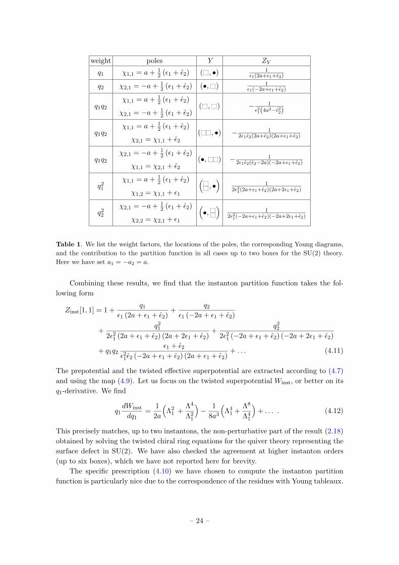
namely [1, 1], and hence one single surface operator to consider [34]. In Tab. 1 we list the

explicit results for this case, including the location of the poles and the contribution due

to all the relevant Young tableaux configurations up to two boxes.

9The sign in this formula is the one that, given our conventions, is consistent with the standard field

theory results.

– 23 –

weight poles Y ZY

q1 χ1,1 = a+ 12 (ε1 + ε2) ( , •) 1

ε1(2a+ε1+ε2)

q2 χ2,1 = −a+ 12 (ε1 + ε2) (•, ) 1

ε1(−2a+ε1+ε2)

q1q2

χ1,1 = a+ 12 (ε1 + ε2)

χ2,1 = −a+ 12 (ε1 + ε2)

( , ) − 1ε21(4a2−ε22)

q1q2

χ1,1 = a+ 12 (ε1 + ε2)

χ2,1 = χ1,1 + ε2( , •) − 1

2ε1ε2(2a+ε2)(2a+ε1+ε2)

q1q2

χ2,1 = −a+ 12 (ε1 + ε2)

χ1,1 = χ2,1 + ε2(•, ) − 1

2ε1ε2(ε2−2a)(−2a+ε1+ε2)

q21

χ1,1 = a+ 12 (ε1 + ε2)

χ1,2 = χ1,1 + ε1

(, •)

12ε21(2a+ε1+ε2)(2a+2ε1+ε2)

q22

χ2,1 = −a+ 12 (ε1 + ε2)

χ2,2 = χ2,1 + ε1

(•,

)1

2ε21(−2a+ε1+ε2)(−2a+2ε1+ε2)

Table 1. We list the weight factors, the locations of the poles, the corresponding Young diagrams,

and the contribution to the partition function in all cases up to two boxes for the SU(2) theory.

Here we have set a1 = −a2 = a.

Combining these results, we find that the instanton partition function takes the fol-

lowing form

Zinst[1, 1] = 1 +q1

ε1 (2a+ ε1 + ε2)+

q2

ε1 (−2a+ ε1 + ε2)

+q2

1

2ε21 (2a+ ε1 + ε2) (2a+ 2ε1 + ε2)+

q22

2ε21 (−2a+ ε1 + ε2) (−2a+ 2ε1 + ε2)

+ q1q2ε1 + ε2

ε21ε2 (−2a+ ε1 + ε2) (2a+ ε1 + ε2)+ . . . (4.11)

The prepotential and the twisted effective superpotential are extracted according to (4.7)

and using the map (4.9). Let us focus on the twisted superpotential Winst, or better on its

q1-derivative. We find

q1dWinst

dq1=

1

2a

(Λ2

1 +Λ4

Λ21

)− 1

8a3

(Λ4

1 +Λ8

Λ41

)+ . . . . (4.12)

This precisely matches, up to two instantons, the non-perturbative part of the result (2.18)

obtained by solving the twisted chiral ring equations for the quiver theory representing the

surface defect in SU(2). We have also checked the agreement at higher instanton orders

(up to six boxes), which we have not reported here for brevity.

The specific prescription (4.10) we have chosen to compute the instanton partition

function is particularly nice due to the correspondence of the residues with Young tableaux.

– 24 –

However, there are many other possible choices of contours that one can make. One way to

classify these distinct contours is using the Jeffrey-Kirwan (JK) prescription [35]. In this

terminology, the set of poles chosen to compute the residues is described by a JK parameter

η, which is a particular linear combination of the χI,s; the prescription chooses a set of

factors D from the denominator of zdI such that, if we only consider the χI,s-dependent

terms of these chosen factors, then, η can be written as a positive linear combination of

these. For instance, our prescription in (4.10) corresponds to choosing 10

η = −M∑I=1

χI (4.13)

For a detailed discussion of this method in the context of ramified instantons we refer to

[7] where it is also shown that different JK prescriptions can be mapped to different quiver

realizations of the surface operator.

Let us consider for example the prescription corresponding to a JK parameter of the

form

η = −M−1∑I=1

χI + ζ χM (4.14)

where ζ is a large positive number. In our notation this corresponds to closing the inte-

gration contours in the upper half-plane as before for the first (M − 1) variables, and in

the lower half plane for χM . Applying this new prescription to the SU(2) theory, we find

a different set of poles that contribute. They are explicitly listed in Tab. 2.

Comparing with Tab. 1, we see that, although the location of residues has changed, for

most cases the residues are unchanged. The only set of residues that give an apparently

different answer is the one with d1 = d2 = 1 with weight q1q2. As opposed to the earlier

case, where there were three contributions, now there are only two terms proportional

to q1q2. However, it is easy to see that if we sum these contributions, we find an exact

match between the two prescriptions. This fact should not come as surprise since it is

a simple consequence of the residue theorem applied to the χ2 integral. Therefore, all

results that follow from the instanton partition function (and in particular the twisted

superpotential) are the same in the two cases. Of course what we have just seen in the

simple SU(2) case at the two instanton level, occurs also at higher instanton numbers and

with higher rank gauge groups. The price one pays in changing the contour prescription

or equivalently in changing the JK parameter from (4.13) to (4.14) is the loss of a simple

one-to-one correspondence with the Young tableaux, but the gain is that, as shown in [7],

the second prescription produces at each instanton order an instanton partition that is

already organized in a factorized form in which the various factors account for the 2d, the

4d and the mixed 2d/4d contributions. This is a feature that will play a fundamental role

in the 3d/5d extension.

Let us now list our findings obtained by using the second residue prescription for the

SU(3) theory, limiting ourselves to the one-instanton terms for brevity. In the case of the

10We understand the extra index s running from 1 to nI .

– 25 –

weight poles ZY

q1 χ1,1 = a+ 12 (ε1 + ε2) 1

ε1(2a+ε1+ε2)

q2 χ2,1 = a− 12 (ε1 + ε2) 1

ε1(−2a+ε1+ε2)

q1q2

χ1,1 = χ2,1 + ε2

χ2,1 = −a− 12(ε1 + 3ε2)

− 12ε1ε2(2a+ε2)(2a+ε1+ε2)

q1q2

χ1,1 = χ2,1 + ε2

χ2,1 = a− 12(ε1 + ε2)

ε1+2ε22ε21ε2(2a+ε2)(−2a+ε1+ε2)

q21

χ1,1 = a1 + 12 (ε1 + ε2)

χ1,2 = χ1,1 + ε1

12ε21(2a+ε1+ε2)(2a+2ε1+ε2)

q22

χ2,1 = a− 12 (ε1 + ε2)

χ2,2 = χ2,1 − ε11

2ε21(−2a+ε1+ε2)(−2a+2ε1+ε2)

Table 2. We list the weight factors, the pole structure and the contribution to the partition function

in all cases up to two boxes for the SU(2) theory using the contour prescription corresponding to

the JK parameter (4.14).

surface operator corresponding to the partition [1,2] we get

Zinst[1, 2] = 1 +q1

ε1 (a12 + ε1 + ε2) (a13 + ε1 + ε2)+

q2

ε1 (a21 + ε1 + ε2) (a31 + ε1 + ε2)+ . . .

(4.15)

while for the surface operator described by the partition [1,1,1] we obtain

Zinst[1, 1, 1] = 1 +q1

ε1 (a12 + ε1 + ε2)+

q2

ε1 (a23 + ε1 + ε2)+

q3

ε1 (a31 + ε1 + ε2)+ . . . .

(4.16)

Applying (4.7) to extract Winst, we find that the qI -logarithmic derivatives of the twisted

superpotential for the two partitions perfectly match the non-perturbative pieces of the

solutions (2.57) and (2.58) of the twisted chiral ring equations. We have checked that

this agreement persists at the two-instanton level. We have also thoroughly explored all

surface operators in the SU(4) theory and many cases in higher rank theories up to two

instantons, always finding a perfect match between the qI -logarithmic derivatives of W and

the solutions of the corresponding twisted chiral ring equations.

4.2 Localization in 5d

We now turn to discuss the results for a gauge theory on R4 × S1β in the presence of a

surface operator also wrapping the compactification circle. This case has been discussed

by a number of recent works (see for instance [36, 37]).

Here we observe that the ramified instanton partition function is given by the same

expressions (4.2) and (4.3) in which the function g(x) is [23, 24, 38]

g(x) = 2 sinhβx

2(4.17)

– 26 –

Another difference with respect to the 2d/4d case is that the counting parameters qI are

now dimensionless and are given by

qI = (−1)kI−1(βΛI

)bI for I = 1, . . . ,M − 1 ,

qM = (−1)N(βΛ)2N(M−1∏

I=1

qI

)−1.

(4.18)

The final result is obtained by summing the residues of zdI over the same set of poles

selected by the JK prescription (4.14).

Let us illustrate these ideas by calculating the twisted effective superpotential that

governs the infrared behavior of the [1, 1] operator in SU(2). Up to two instantons, the

partition function using these rules is

Zinst.[1, 1] = 1 +q1

4 sinh(β

2 ε1)

sinh(β

2 (2a+ ε1 + ε2)) +

q2

4 sinh(β

2 ε1)

sinh(β

2 (−2a+ ε1 + ε2))

+q2

1

16 sinh(β

2 ε1)

sinh(βε1)

sinh(β

2 (2a+ ε1 + ε2))

sinh(β

2 (2a+ 2ε1 + ε2))

+q2

2

16 sinh(β

2 ε1)

sinh(βε1)

sinh(β

2 (−2a+ ε1 + ε2))

sinh(β

2 (−2a+ 2ε1 + ε2))

+q1q2 sinh

(β2 (ε1 + 2ε2)

)16 sinh2

(β2 ε1)

sinh(βε2)

sinh(β

2 (−2a+ ε1 + ε2))

sinh(β

2 (2a+ ε2))

+q1q2

16 sinh(β

2 ε1)

sinh(βε2)

sinh(β

2 (2a+ ε1 + ε2))

sinh(β

2 (2a+ ε2))

+ . . . (4.19)

where a1 = −a2 = a. From this instanton partition function we can extract the twisted

chiral superpotential in the usual manner according to (4.7). The result is

q1dWinst

dq1=

β

2 sinh(βa)

(Λ2

1 +Λ4

Λ21

)− β3 cosh(βa)

8 sinh3(βa)

(Λ4

1 +Λ8

Λ41

)+ . . . (4.20)

It is very easy to check that in the limit β → 0 this expression reduces to the 2d/4d result

in (4.12). Most importantly it agrees with the non-perturbative part of the solution (3.32)

of the chiral ring equation of the 3d/5d SU(2) theory, thus confirming the validity of (3.27).

Similar calculations can be performed for the higher rank cases without much difficulty,

and indeed we have done these calculations for all surface operators of SU(4) and for many

cases up to SU(6). Here, for brevity, we simply report the results at the one-instanton level

for the surface operators in the SU(3) theory. In the case of the defect of type [1,2] the

instanton partition function is

Zinst[1, 2] = 1 +q1

8 sinh(β

2 ε1)

sinh(β

2 (a12 + ε1 + ε2))

sinh(β

2 (a13 + ε1 + ε2)) (4.21)

+q2

8 sinh(β

2 ε1)

sinh(β

2 (−a12 + ε1 + ε2))

sinh(β

2 (−a13 + ε1 + ε2)) + . . . ,

– 27 –

while for the defect of type [1,1,1] we find

Zinst[1, 1, 1] = 1 +q1

4 sinh(β

2 ε1)

sinh(β

2 (a12 + ε1 + ε2)) +

q2

4 sinh(β

2 ε1)

sinh(β

2 (a23 + ε1 + ε2))

+q3

4 sinh(β

2 ε1)

sinh(β

2 (a31 + ε1 + ε2)) + . . . (4.22)

where aij = a1 − aj . These expressions are clear generalizations of the 2d/4d instanton

partition functions (4.15) and (4.16). Moreover one can check that the twisted superpo-

tentials that can be derived from them perfectly match the ones obtained by solving the

chiral ring equations as we discussed in Section 3.

5 Superpotentials for dual quivers

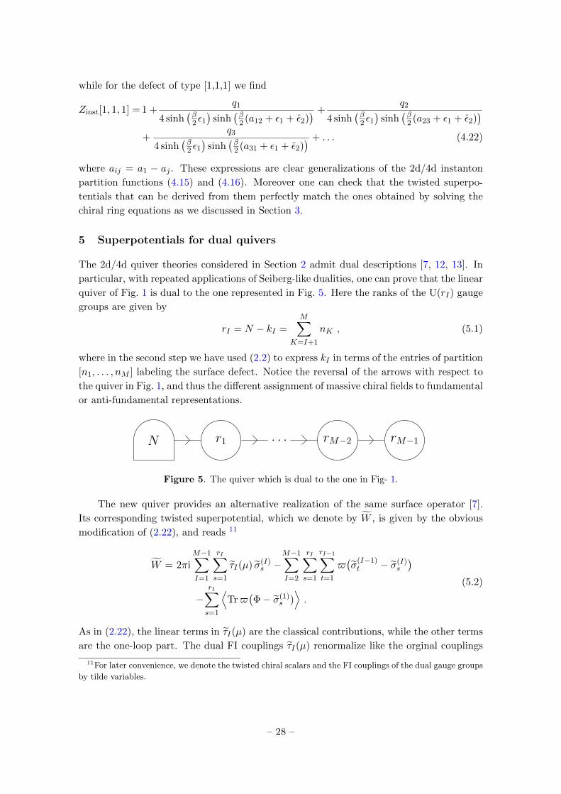
The 2d/4d quiver theories considered in Section 2 admit dual descriptions [7, 12, 13]. In

particular, with repeated applications of Seiberg-like dualities, one can prove that the linear

quiver of Fig. 1 is dual to the one represented in Fig. 5. Here the ranks of the U(rI) gauge

groups are given by

rI = N − kI =M∑

K=I+1

nK , (5.1)

where in the second step we have used (2.2) to express kI in terms of the entries of partition

[n1, . . . , nM ] labeling the surface defect. Notice the reversal of the arrows with respect to

the quiver in Fig. 1, and thus the different assignment of massive chiral fields to fundamental

or anti-fundamental representations.

N r1 . . . rM−2 rM−1

Figure 5. The quiver which is dual to the one in Fig- 1.

The new quiver provides an alternative realization of the same surface operator [7].

Its corresponding twisted superpotential, which we denote by W , is given by the obvious

modification of (2.22), and reads 11

W = 2πi

M−1∑I=1

rI∑s=1

τI(µ) σ(I)s −

M−1∑I=2

rI∑s=1

rI−1∑t=1

$(σ

(I−1)t − σ(I)

s

)−

r1∑s=1

⟨Tr$

(Φ− σ(1)

s )⟩.

(5.2)

As in (2.22), the linear terms in τI(µ) are the classical contributions, while the other terms

are the one-loop part. The dual FI couplings τI(µ) renormalize like the orginal couplings

11For later convenience, we denote the twisted chiral scalars and the FI couplings of the dual gauge groups

by tilde variables.

– 28 –

τI(µ) but with kI replaced by rI . In view of (5.1), this implies that the one-loop β-function

coefficient in the dual theory is opposite to that of the original theory, namely

bI = rI+1 − rI−1 = −kI+1 + kI−1 = −bI . (5.3)

In turn, this implies that the dynamically generated scale in the I-th node of the dual

theory is given by

ΛbII = e−2πi τI µbI , (5.4)

to be compared with (2.27). As usual we can trade the couplings τI(µ) for these scales

ΛI , and thus rewrite the twisted superpotential (5.2) in a form that is the straightforward

modification of (2.29).

If we make the following classical ansatz

σ(I) = diag(an1+...+nI+1, an1+...+nI+2, . . . , aN ) , (5.5)

which is dual to the one for σ(I) given in (2.41), then it is easy to check that

Tr σ(I) = −Trσ(I) . (5.6)

This clearly implies

1

2πi

∂Wclass

∂τI= − 1

2πi

∂Wclass

∂τI. (5.7)

Thus, if the FI parameters in the two dual models are related to each other by

τI = −τI , (5.8)

one has Wclass = Wclass. Notice that using (5.8) in (5.4) and comparing with (2.27), we

have

ΛI = ΛI . (5.9)

The relation (5.6) remains true also at the quantum level. This statement can be

verified by expanding σ(I) as a power series in the various ΛI ’s around the classical vacuum

(5.5), and iteratively solving the corresponding chiral ring equations in a semi-classical

approximation. Doing this and using (5.8) and (5.9), we have checked the validity of

(5.6) in several examples. Furthermore, we have obtained the same relations also using

the localization methods described in Section 4. Therefore, we can conclude that the two

quiver theories in Fig. 1 and 5, indeed provide equivalent descriptions of the 2d/4d defect

SU(N)[n1, . . . , nM ].

This conclusion changes drastically once we consider the 3d/5d quiver theories com-

pactified on a circle. In this case, the dual superpotential corresponding to the quiver in

Fig. 5, is obtained by upgrading (5.2) to a form analogous to (3.8), namely

W =M−1∑I=1

rI∑s=1

bI log(βΛI)σ(I)s −

M−1∑I=2

rI∑s=1

rI−1∑t=1

`(σ

(I−1)t − σ(I)

s

)−

r1∑s=1

⟨Tr `

(Φ− σ(1)

s

)⟩.

(5.10)

– 29 –

Here we have used the loop-function `(x) defined in (3.3), and taken into account the

renormalization of the FI couplings to introduce the scales ΛI . Using for the original

quiver the ansatz (3.25), and for the dual theory the ansatz (5.5), which can be rewritten

as

S(I) = diag(An1+...+nI+1 , An1+...+nI+2 , . . . , AN ) (5.11)

in terms of the exponential variables S(I) = eβσ(I)

and Ai = eβai , one can easily check that

the relation (5.6) still holds true.

However, in general, this is no longer valid for the full solutions of the chiral ring

equations. This happens whenever the ranks kI of the original quiver theory and the ranks

rI of the dual model are different from each other for some I, which is the generic situation.

Let us show this in a specific example, namely the defect of type [1,2] in the SU(3) theory.

The original quiver theory was discussed in detail in Section 3 where we have shown that

the solution of the chiral ring equation is (see (3.36))

σ? = a1 + β2 A1/21

A12A13

(Λ3

1 +Λ6

Λ31

)+ . . . . (5.12)

The dual quiver for this defect is depicted in Fig. 6.

3 2

Figure 6. The dual quiver for the SU(3)[1, 2] defect.

From (5.10), it follows that the corresponding twisted superpotential is

W =2∑s=1

[− 3

2πilog(βΛ1)σs −

⟨Tr `(Φ− σs)

⟩]. (5.13)

Using the function P3 defined in (3.35), we see that the twisted chiral ring equations are

P3(Ss) = β3(

Λ31 +

Λ6

Λ31

)(5.14)

for s = 1, 2. Solving iteratively these equations around the classical vacuum (5.5), we find

Tr σ? = a2 + a3 + β2(

Λ31 +

Λ6

Λ31

)( A1/23

A13A23− A

1/22

A12A23

)+ . . . . (5.15)

By comparing (5.12) and (5.15), we see that at the classical level Tr σ? is equal to negative

of the solution σ? in the original quiver; this simply follows from the SU(3) tracelessness

condition. However, the first semi-classical correction of order β2 spoils this relation,

even if we use the relation (5.9) between the dynamically generated scales. Therefore, as

anticipated, the two descriptions are not any more dual to each other.

– 30 –

It is interesting to observe that the twisted superpotential corresponding to the dual

solution (5.15) can also be obtained using localization. Indeed, if one evaluates the in-

stanton partition function Zinst[1, 2] for the compactified theory using the JK prescription

with

η = +χ1 − ξ χ2 , (5.16)

where ξ is positive and large, and then extracts from it the corresponding twisted superpo-

tential using (4.7), one obtains precisely the above result 12. Notice that the JK parameter

(5.16) is opposite in sign with respect to the one in (4.14) that we have adopted in the

original quiver realization. Actually, what we have seen in this particular example can be

generalized to other cases and for any M , we find that the JK parameter which has to be

used in the localization computations for the dual quiver theory to match the solution of

the chiral ring equations is

η =M−1∑I=1

χI − ξ χM . (5.17)

This fact points towards the nice scenario in which the twisted superpotentials W and W

for a pair of quiver theories related by a chain of Seiberg-like dualities can be obtained

in localization using two different JK prescriptions associated to opposite η parameters.

While in the 2d/4d systems all different JK prescriptions are equivalent to each other and

lead to the same superpotentials, in general this is no longer true in the 3d/5d theories

because of the particular structure of the instanton partition functions.

5.1 Adding Chern-Simons terms

We now investigate the possibility of restoring the duality between the two 3d/5d descrip-

tions of the SU(3)[1,2] defect by considering the addition of Chern-Simons (CS) couplings.

These can be written as a term in the twisted chiral superpotential that is quadratic in

the twisted scalars and proportional to the compactification circle β [14, 39]. For the Ith

node, the CS term is of the form:

WCS =k

2β Tr (σ(I))2 . (5.18)

Let us start from the original theory and let us turn on a CS term on the U(1) node

with coupling k. The resulting quiver is represented in Fig. 7 and the corresponding twisted

superpotential is

W = 3 log(βΛ1)σ +k

2β σ2 −

⟨Tr `(σ − Φ)

⟩. (5.19)

Repeating the same steps described in Section 3, we easily obtain the modified twisted

chiral ring equation

P3(S) = β3(SkΛ3

1 +Λ6

SkΛ31

)(5.20)

12We have checked this up to the two-instanton level, namely up to order β5.

– 31 –

1k 3

Figure 7. The quiver for the SU(3)[1,2] theory with a CS term with coupling k on the U(1) node.

where, as before, P3 is given in (3.35) and S = eβσ. Solving this equation with the usual

ansatz leads to

σ? = a1 + β2 A1/21

A12A13

(Ak1 Λ3

1 +Λ6

Ak1 Λ31

)+ . . . . (5.21)

Of course, for k = 0 one recovers the solution (5.12) in the absence of the CS term.

Let us now consider the dual quiver with a CS interaction with coupling k turned on

in the U(2) node.

3 2k

Figure 8. The quiver representing the dual realization of the SU(3)[1,2] with a CS term on the

U(2) node

This is represented in Fig. 8 and the corresponding twisted superpotential is

W =2∑s=1

[− 3 log(βΛ1) σs +

k

2β σ2

s −⟨

Tr `(Φ− σs)⟩]

. (5.22)

From this we can easily derive the twisted chiral ring equations, namely

P3(Ss) = β3( Λ3

1

Sks+Sks Λ6

Λ31

)(5.23)

for s = 1, 2, which are a simple generalization of (5.14). Solving these equations with the

ansatz (5.5) we find

σ?,1 + σ?,2 = a2 + a3 + β2

[(A1/2−k3

A13A23− A

1/2−k2

A12A23

)Λ3

1+(A1/2+k

3

A13A23− A

1/2+k2

A12A23

)Λ6

Λ31

]+ . . . .

(5.24)

Of course for k = 0 we recover the solution (5.15) in the absence of the CS coupling.

Our main observation is that if we take

k = −k =1

2(5.25)

then, using the SU(3) tracelessness condition and the relations (5.8) and (5.9), we have

σ?,1 + σ?,2 = −σ? (5.26)

– 32 –

This implies that

Λ1dW

dΛ1

= −Λ1dW

dΛ1, (5.27)

so that the duality between W and W is restored at the quantum level under the map

(5.8) and (5.9). We have checked that this match holds true at the next-order in the β-

expansion of the solutions of the chiral ring equations. Therefore, thanks to the CS terms

also in the 3d/5d case we can realize the same kind of relation which was manifest in the

2d/4d theories.

In Appendix B, we discuss a slightly more complicated example in which a similar

phenomenon occurs. It is a surface operator of type [1,1,2] in the SU(4) gauge theory

compactified on S1β. In this case as well, the two dual quivers lead to the same twisted

chiral superpotential provided suitable CS couplings are turned on.

6 Conclusions and perspectives

In this paper we have studied surface operators in four- and five-dimensional SU(N) gauge

theories, focusing on the effective twisted chiral superpotential which governs their infrared

dynamics. Our results are a natural generalization and extension of those in [10].

We have illustrated our findings in the context of the simplest defects in SU(2) and

SU(3) theories, even though we have performed several checks in a number of theories

with higher rank gauge groups. Already in the simplest SU(3) case we could observe that

different realizations of the same surface operator in terms of dual quivers lead, in the

five-dimensional case, to different twisted superpotentials. We have found that this feature

is reproduced also in the localization approach where the different superpotentials arise

from different choices of the Jeffrey-Kirwan residue prescription. In an interesting twist,

we have shown that the duality between the coupled 3d/5d quivers can be restored by the

addition of suitable three-dimensional Chern-Simons terms. Clearly, it would be desirable

to do a systematic analysis of this phenomenon and thoroughly explore the effects of the

Chern-Simons couplings, but we leave this to future work.

It would be very interesting to extend our results to surface operators in N = 2?

theories. As shown in our earlier work [6], the non-perturbative S-duality group of the

four-dimensional theory constrains the twisted superpotential of the monodromy defect,

which can be written in terms of elliptic and modular forms in a semi-classical expansion.

Therefore, it would be worthwhile to understand if it is possible to obtain these exact

results directly from the chiral ring analysis of a coupled quiver gauge theories and also to

extend them to five dimensions.

Surface operators in four- and five-dimensional gauge theories have been studied also

by exploiting their connections to integrable systems and in particular the relation between

the twisted chiral ring equations and Bethe ansatz for integrable spin chains [14–16]. In this

context, the wave-functions of the quantum systems can be related to the instanton parti-

tion function in the presence of surface operators [40, 41]. For the 3d/5d theories studied

in this work, recently there has been interesting developments on the connection between

the instanton partition function and the wave functions of relativistic Toda theories [42].

– 33 –

It would be worthwhile to explore this direction using our methods. Another interesting

possibility is to use dualities between three-dimensional quiver gauge theories with flavor

to study bi-spectral dualities between quantum integrable systems [11]. It would be de-

sirable to investigate the possible implications of our results for these integrable systems,

especially in the presence of Chern-Simons couplings.

Acknowledgments

We would like to thank Sourav Ballav, Noppadol Mekareeya, Madhusudhan Raman

and Jan Troost for many useful discussions. S.K.A. would especially like to thank for the

hospitality the Physics Department of the University of Torino and the Torino Section of

INFN where this work was initiated.

The work of M.B., M.F. and A.L. is partially supported by the MIUR PRIN Contract

2015MP2CX4 “Non-perturbative Aspects Of Gauge Theories And Strings”.

A Chiral correlators in 5d

In this appendix we briefly review some well-known results about the way in which chiral

correlators are computed using localization [43–45] that are useful for the calculations

presented in the main text. For details we refer to [46] and references therein.

In a four-dimensional theory SU(N) the generating function of all chiral correlators of

the form⟨Tr Φ`

⟩is

⟨Tr ezΦ

⟩=

N∑i=1

ezai − 1

Zinst

∞∑k=1

qk

k!

∫ k∏I=1

dχI2πi

zk(χI)O(z, χI) (A.1)

where zk(χI) is the k-instanton partition function and O is the following observable

O(z, χI) =k∑I=1

exχI (1− ezε1)(1− ezε2) . (A.2)

Rather interestingly, the same formula (A.1) can also be exploited to compute the quantum

corrected correlators in the five-dimensional SU(N) theory provided one uses the appro-

priate function g(x) as in (4.17) and sets z = `β for ` ∈ Z and ` < N .

With an explicit calculation, we find the following universal formula

V` ≡⟨

Tr e`βΦ⟩

=N∑i=1

A`i + `2(βΛ)2NN∑i=1

AN−2+`i∏

j 6=i(Ai −Aj)2+O

((βΛ)4N

)(A.3)

where Ai = eβai . Once the V` are obtained, the U`’s which appear in the five-dimensional

Seiberg-Witten curve can be calculated by forming the symmetric polynomials in the usual

manner. In particular, we have U1 = V1 and UN−1 = V−1. The last relation follows

– 34 –

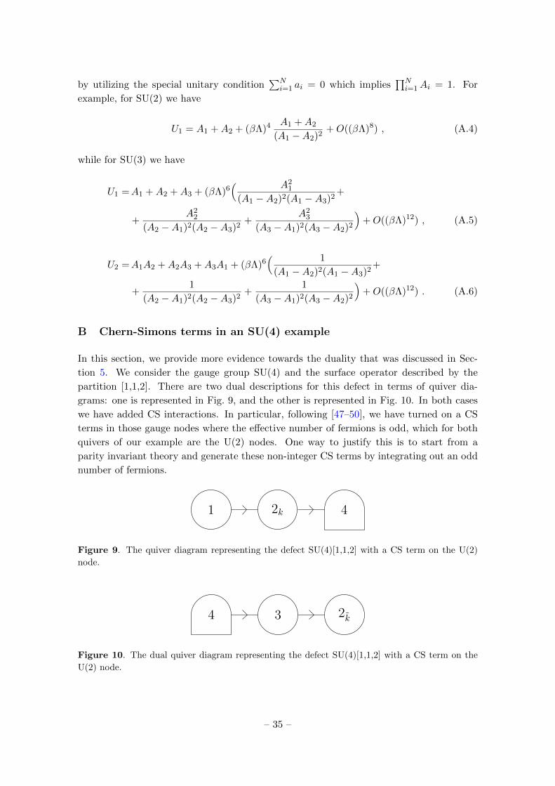
by utilizing the special unitary condition∑N

i=1 ai = 0 which implies∏Ni=1Ai = 1. For

example, for SU(2) we have

U1 = A1 +A2 + (βΛ)4 A1 +A2

(A1 −A2)2+O((βΛ)8) , (A.4)

while for SU(3) we have

U1 =A1 +A2 +A3 + (βΛ)6( A2

1

(A1 −A2)2(A1 −A3)2+

+A2

2

(A2 −A1)2(A2 −A3)2+

A23

(A3 −A1)2(A3 −A2)2

)+O((βΛ)12) , (A.5)

U2 =A1A2 +A2A3 +A3A1 + (βΛ)6( 1

(A1 −A2)2(A1 −A3)2+

+1

(A2 −A1)2(A2 −A3)2+

1

(A3 −A1)2(A3 −A2)2

)+O((βΛ)12) . (A.6)

B Chern-Simons terms in an SU(4) example

In this section, we provide more evidence towards the duality that was discussed in Sec-

tion 5. We consider the gauge group SU(4) and the surface operator described by the

partition [1,1,2]. There are two dual descriptions for this defect in terms of quiver dia-

grams: one is represented in Fig. 9, and the other is represented in Fig. 10. In both cases

we have added CS interactions. In particular, following [47–50], we have turned on a CS

terms in those gauge nodes where the effective number of fermions is odd, which for both

quivers of our example are the U(2) nodes. One way to justify this is to start from a

parity invariant theory and generate these non-integer CS terms by integrating out an odd

number of fermions.

1 2k 4

Figure 9. The quiver diagram representing the defect SU(4)[1,1,2] with a CS term on the U(2)

node.

4 3 2k

Figure 10. The dual quiver diagram representing the defect SU(4)[1,1,2] with a CS term on the

U(2) node.

– 35 –

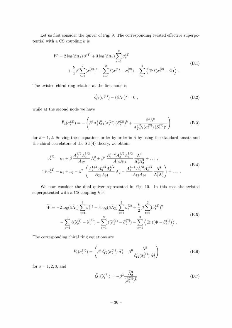
Let us first consider the quiver of Fig. 9. The corresponding twisted effective superpo-

tential with a CS coupling k is

W = 2 log(βΛ1)σ(1) + 3 log(βΛ2)2∑s=1

σ(2)s

+k

2β

2∑t=1

(σ(2)t )2 −

2∑t=1

`(σ(1) − σ(2)t )−

2∑t=1

⟨Tr `(σ

(2)t − Φ)

⟩.

(B.1)

The twisted chiral ring relation at the first node is

Q2(σ(1))− (βΛ1)2 = 0 , (B.2)

while at the second node we have

P4(σ(2)s ) = −

(β3Λ3

2 Q1(σ(2)s ) (S(2)

s )k +β5Λ8

Λ32Q1(σ

(2)s ) (S

(2)s )k

)(B.3)

for s = 1, 2. Solving these equations order by order in β by using the standard ansatz and

the chiral correlators of the SU(4) theory, we obtain

σ(1)? = a1 + β

A1/21 A

1/22

A12Λ2

1 + β2 A1−k1 A

1/23 A

1/24

A13A14

Λ8

Λ21Λ3

2

+ . . . ,

Trσ(2)? = a1 + a2 − β2

(A1+k

2 A1/23 A

1/24

A23A24Λ3

2 −A1−k

1 A1/23 A

1/24

A13A14

Λ8

Λ21Λ3

2

)+ . . . .

(B.4)

We now consider the dual quiver represented in Fig. 10. In this case the twisted

superpotential with a CS coupling k is

W = −2 log(βΛ1)

3∑s=1

σ(1)s − 3 log(βΛ2)

2∑t=1

σ(2)t +

k

2β

2∑t=1

(σ(2)t )2

−3∑s=1

`(σ(1)s − σ

(2)1 )−

3∑s=1

`(σ(1)s − σ

(2)2 )−

3∑s=1

⟨Tr `(Φ− σ(1)

s )⟩.

(B.5)

The corresponding chiral ring equations are

P4(σ(1)s ) =

(β2 Q2(σ(1)

s ) Λ21 + β6 Λ8

Q2(σ(1)s ) Λ2

1

)(B.6)

for s = 1, 2, 3, and

Q1(σ(2)t ) = −β3 Λ3

2

(S(2)t )k

(B.7)

– 36 –

for t = 1, 2. Solving these equations with the usual ansatz, we find

Tr σ(1)? = a2 + a3 + a4 − β

A1/21 A

1/22

A12Λ2

1

+ β2

(A

1/21 A1+k

3 A1/24

A31A34+A−k−1/21 A−k−1

2 A−k−1/23

A41A43

)Λ8

Λ21Λ3

2

+ . . . ,

(B.8)

Tr σ(2)∗ = a3 + a4 − β2

(A

1/22 A1−k

3 A1/24

A32A34+Ak−1

1 A−1/2+k2 A

−1/2+k3

A42A43

)Λ3

2

+ β2

(A

1/21 A1+k

3 A1/24

A31A34+A−1/2−k1 A−k−1

2 A−1/2−k3

A14A34

)Λ8

Λ21Λ3

2

+ . . . .

These expressions look very different from the solution (B.4) of the chiral ring equations

of the original quiver. However, if we impose the SU(4) tracelessness constraint∑

i ai = 0

and use the following map

k = −k =1

2and ΛI = ΛI , (B.9)

we find the following relations

Tr σ(1)? = −σ(1)

? ,

Tr σ(2)? = −Trσ

(2)? .

(B.10)

This proves that, to leading order in the instanton expansion, the superpotentials of the

dual pair match as expected. We have checked that this match continues to hold up to two

instantons as well.

References

[1] S. Gukov, Surface Operators, New Dualities of Supersymmetric Gauge Theories, 223-259,

2016, arXiv:1412.7127.

[2] S. Gukov and E. Witten, Gauge Theory, Ramification, And The Geometric Langlands

Program, hep-th/0612073.

[3] S. Gukov and E. Witten, Rigid Surface Operators, Adv. Theor. Math. Phys. 14 (2010), no. 1

87–178, [arXiv:0804.1561].

[4] H. Kanno and Y. Tachikawa, Instanton counting with a surface operator and the chain-saw

quiver, JHEP 06 (2011) 119, [arXiv:1105.0357].

[5] S. Nawata, Givental J-functions, Quantum integrable systems, AGT relation with surface

operator, Adv. Theor. Math. Phys. 19 (2015) 1277–1338, [arXiv:1408.4132].

[6] S. K. Ashok, M. Billo, E. Dell’Aquila, M. Frau, R. R. John, and A. Lerda, Modular and

duality properties of surface operators in N=2* gauge theories, JHEP 07 (2017) 068,

[arXiv:1702.02833].

[7] A. Gorsky, B. Le Floch, A. Milekhin, and N. Sopenko, Surface defects and instanton–vortex

interaction, Nucl. Phys. B920 (2017) 122–156, [arXiv:1702.03330].

– 37 –

[8] D. Gaiotto, Surface Operators in N = 2 4d Gauge Theories, JHEP 11 (2012) 090,

[arXiv:0911.1316].

[9] J. Gomis and B. Le Floch, M2-brane surface operators and gauge theory dualities in Toda,

JHEP 04 (2016) 183, [arXiv:1407.1852].

[10] D. Gaiotto, S. Gukov, and N. Seiberg, Surface Defects and Resolvents, JHEP 09 (2013) 070,

[arXiv:1307.2578].

[11] D. Gaiotto and P. Koroteev, On Three Dimensional Quiver Gauge Theories and

Integrability, JHEP 05 (2013) 126, [arXiv:1304.0779].

[12] F. Benini, D. S. Park, and P. Zhao, Cluster Algebras from Dualities of 2d N = (2, 2) Quiver

Gauge Theories, Commun. Math. Phys. 340 (2015) 47–104, [arXiv:1406.2699].

[13] C. Closset, S. Cremonesi, and D. S. Park, The equivariant A-twist and gauged linear sigma

models on the two-sphere, JHEP 06 (2015) 076, [arXiv:1504.06308].

[14] N. A. Nekrasov and S. L. Shatashvili, Supersymmetric vacua and Bethe ansatz, Nucl. Phys.

Proc. Suppl. 192-193 (2009) 91–112, [arXiv:0901.4744].

[15] N. A. Nekrasov and S. L. Shatashvili, Quantum integrability and supersymmetric vacua,

Prog. Theor. Phys. Suppl. 177 (2009) 105–119, [arXiv:0901.4748].

[16] N. A. Nekrasov and S. L. Shatashvili, Quantization of Integrable Systems and Four

Dimensional Gauge Theories, Proceedings, 16th International Congress on Mathematical

Physics (ICMP09): Prague, Czech Republic, August 3-8, 2009 arXiv:0908.4052.

[17] A. Hanany and K. Hori, Branes and N=2 theories in two-dimensions, Nucl. Phys. B513

(1998) 119–174, [hep-th/9707192].

[18] E. Witten, Phases of N=2 theories in two-dimensions, Nucl. Phys. B403 (1993) 159–222,

[hep-th/9301042].

[19] F. Cachazo, M. R. Douglas, N. Seiberg, and E. Witten, Chiral rings and anomalies in

supersymmetric gauge theory, JHEP 12 (2002) 071, [hep-th/0211170].

[20] E. D’Hoker, I. M. Krichever, and D. H. Phong, The Effective prepotential of N=2

supersymmetric SU(N(c)) gauge theories, Nucl. Phys. B489 (1997) 179–210,

[hep-th/9609041].

[21] S. G. Naculich, H. J. Schnitzer, and N. Wyllard, The N = 2 U(N) gauge theory prepotential

and periods from a perturbative matrix model calculation, Nucl. Phys. B651 (2003) 106–124,

[hep-th/0211123].

[22] N. Nekrasov, Five dimensional gauge theories and relativistic integrable systems, Nucl. Phys.

B531 (1998) 323–344, [hep-th/9609219].

[23] N. Nekrasov, Seiberg-Witten prepotential from instanton counting, Adv. Theor. Math. Phys.

7 (2004) 831–864, [hep-th/0206161].

[24] N. Nekrasov and A. Okounkov, Seiberg-Witten theory and random partitions, Prog. Math.

244 (2006) 525–596, [hep-th/0306238].

[25] M. Wijnholt, Five-dimensional gauge theories and unitary matrix models, hep-th/0401025.

[26] L. F. Alday and Y. Tachikawa, Affine SL(2) conformal blocks from 4d gauge theories, Lett.

Math. Phys. 94 (2010) 87–114, [arXiv:1005.4469].

– 38 –

[27] V. Mehta and C. Seshadri, Moduli of Vector Bundles on Curves with Parabolic Structures,

Math. Ann. 248 (1980) 205–240.

[28] I. Biswas, Parabolic bundles as orbifold bundles, Duke Math. J. 88 (1997) 305–325.

[29] B. Feigin, M. Finkelberg, A. Negut, and R. Leonid, Yangians and cohomology rings of

Laumon spaces, math-ag/0812.4656.

[30] L. F. Alday, D. Gaiotto, S. Gukov, Y. Tachikawa, and H. Verlinde, Loop and surface

operators in N=2 gauge theory and Liouville modular geometry, JHEP 1001 (2010) 113,

[arXiv:0909.0945].

[31] G. W. Moore, N. Nekrasov, and S. Shatashvili, D-particle bound states and generalized

instantons, Commun. Math. Phys. 209 (2000) 77–95, [hep-th/9803265].

[32] M. Billo, M. Frau, F. Fucito, A. Lerda, and J. F. Morales, S-duality and the prepotential in

N = 2? theories (I): the ADE algebras, JHEP 11 (2015) 024, [arXiv:1507.07709].

[33] M. Billo, M. Frau, F. Fucito, A. Lerda, and J. F. Morales, S-duality and the prepotential of

N = 2? theories (II): the non-simply laced algebras, JHEP 11 (2015) 026,

[arXiv:1507.08027].

[34] H. Awata, H. Fuji, H. Kanno, M. Manabe, and Y. Yamada, Localization with a Surface

Operator, Irregular Conformal Blocks and Open Topological String, Adv. Theor. Math. Phys.

16 (2012), no. 3 725–804, [arXiv:1008.0574].

[35] L. C. Jeffrey and F. C. Kirwan, Localization for nonabelian group actions, Topology 34

(1995) 291–327.

[36] D. Gaiotto and H.-C. Kim, Surface defects and instanton partition functions, JHEP 10

(2016) 012, [arXiv:1412.2781].

[37] M. Bullimore, H.-C. Kim, and P. Koroteev, Defects and Quantum Seiberg-Witten Geometry,

JHEP 05 (2015) 095, [arXiv:1412.6081].

[38] T. J. Hollowood, A. Iqbal, and C. Vafa, Matrix models, geometric engineering and elliptic

genera, JHEP 03 (2008) 069, [hep-th/0310272].

[39] H.-Y. Chen, T. J. Hollowood, and P. Zhao, A 5d/3d duality from relativistic integrable

system, JHEP 07 (2012) 139, [arXiv:1205.4230].

[40] K. K. Kozlowski and J. Teschner, TBA for the Toda chain, arXiv:1006.2906.

[41] N. Nekrasov, V. Pestun, and S. Shatashvili, Quantum geometry and quiver gauge theories,

arXiv:1312.6689.

[42] A. Sciarappa, Exact relativistic Toda chain eigenfunctions from Separation of Variables and

gauge theory, arXiv:1706.05142.

[43] U. Bruzzo, F. Fucito, J. F. Morales, and A. Tanzini, Multi-instanton calculus and equivariant

cohomology, JHEP 05 (2003) 054, [hep-th/0211108].

[44] A. S. Losev, A. Marshakov, and N. A. Nekrasov, Small instantons, little strings and free

fermions, In Shifman, M. (ed.) et al.: From fields to strings, vol. 1 581-621 hep-th/0302191.

[45] R. Flume, F. Fucito, J. F. Morales, and R. Poghossian, Matone’s relation in the presence of

gravitational couplings, JHEP 0404 (2004) 008, [hep-th/0403057].

[46] S. K. Ashok, M. Billo, E. Dell’Aquila, M. Frau, A. Lerda, M. Moskovic, and M. Raman,

– 39 –

Chiral observables and S-duality in N = 2* U(N) gauge theories, JHEP 11 (2016) 020,

[arXiv:1607.08327].

[47] G. V. Dunne, Aspects of Chern-Simons theory, in Topological Aspects of Low-dimensional

Systems: Proceedings, Les Houches Summer School of Theoretical Physics, Session 69: Les

Houches, France, July 7-31 1998, 1998. hep-th/9902115.

[48] D. Tong, Dynamics of N=2 supersymmetric Chern-Simons theories, JHEP 07 (2000) 019,

[hep-th/0005186].

[49] M. Aganagic, K. Hori, A. Karch, and D. Tong, Mirror symmetry in (2+1)-dimensions and

(1+1)-dimensions, JHEP 07 (2001) 022, [hep-th/0105075].

[50] O. Aharony and D. Fleischer, IR Dualities in General 3d Supersymmetric SU(N) QCD

Theories, JHEP 02 (2015) 162, [arXiv:1411.5475].

– 40 –