JHEP01(2016)045

Published for SISSA by Springer

Received: June 11, 2015

Revised: October 26, 2015

Accepted: December 17, 2015

Published: January 8, 2016

Interference effects in Higgs production through

Vector Boson Fusion in the Standard Model and its

singlet extension

Alessandro Ballestreroa and Ezio Mainaa,b

aINFN, Sezione di Torino,

Via Giuria 1, 10125 Torino, ItalybDipartimento di Fisica, Universita di Torino,

Via Giuria 1, 10125 Torino, Italy

E-mail: ballestrero@to.infn.it, maina@to.infn.it

Abstract: Interference effects play an important role in Electroweak Physics. They are

responsible for the restoration of unitarity at large energies. When, as is often the case,

higher order corrections are only available for some particular subamplitude, interferences

need to be carefully computed in order to obtain the best theoretical prediction. It has been

recently pointed out in gluon fusion that whenever more than one neutral, CP even, scalars

are present in the spectrum large cancellations can occur. We extend these studies to Vector

Boson Scattering, examining interference effects in the Higgs sector in the Standard Model

and its one Higgs Singlet extension. Already in the SM there is a significant difference

between the results obtained considering only s-channel Higgs exchange and those obtained

from the full set of scalar exchange diagrams. In the 1HSM these effects are modulated by

the interference between the two neutral Higgses. The full interference between the heavy

Higgs diagrams and the rest of the amplitude, which is the sum of light Higgs exchange

diagrams and of those diagrams in which no Higgs appear, is very small for values of the

mixing angle compatible with the experimental constraints.

Keywords: Higgs Physics, Beyond Standard Model, Standard Model

ArXiv ePrint: 1506.02257

Open Access, c© The Authors.

Article funded by SCOAP3.doi:10.1007/JHEP01(2016)045

JHEP01(2016)045

Contents

1 Introduction 1

2 The singlet extension of the Standard Model 3

3 New features in PHANTOM 4

4 Notation and details of the calculation 5

5 Higgs mediated Vector Boson Scattering signal in the SM 7

6 Higgs mediated Vector Boson Scattering signal in the 1HSM 9

7 Full processes 11

8 Cancellation of the heavy Higgs interferences 15

9 Conclusions 17

1 Introduction

Now that a resonance has been discovered at about 125 GeV [1, 2], the race is on to

measure all its properties. All studies based on LHC Run I data are consistent with the

hypothesis that the new particle is indeed the Standard Model Higgs boson. The mass

is already known with an uncertainty smaller than two per mill from the latest published

analyses [3, 4] and the signal strengths µi = σi/σiSM, where i runs over the decay channels,

are known to about 10 to 20% [3, 5, 6]. There is still room for more complicated Higgs

sectors but compatibility with experimental results is severely restricting their parameter

space [7]. In Run II, larger luminosity and energy will provide more precise measurements

of the characteristics of the new particle and extend the mass range in which other scalars

can be searched for.

Lately, a lot of attention has been paid to the prospects of detailed studies of off-shell

Higgs contributions, which are larger than could naively be expected [8]. On the one hand,

at large energies, Higgs exchange unitarizes processes like Vector Boson Scattering (VBS)

and fermion pair annihilation to Vector Bosons which would otherwise diverge. On the

other hand, the comparison of off-shell and peak cross sections can provide limits on the

total width of the Higgs [9–15]. Both aspects are sensitive to BSM physics through direct

production of new states and through their contributions in loops.

If additional neutral scalars are present in the physical spectrum, non trivial interfer-

ence effects have been demonstrated in Gluon Gluon Fusion (GGF) processes [16–19].

– 1 –

JHEP01(2016)045

It is quite natural to extend these studies to VBS which has been traditionally regarded

as the ultimate testing ground of the ElectroWeak Symmetry Breaking mechanism. The

ratio of the Higgs production cross section in Vector Boson Fusion (VBF) to the cross

section in gluon fusion grows for larger Higgs masses and, as a consequence, the importance

of VBF as a discovery channel for new scalar resonances of an extended Higgs sector

increases. VBF is not affected by BSM physics through loops [20], therefore it can be argued

that the limits it provides on the Higgs width are less model dependent than those obtained

in GGF. It is well known that interference effects between Higgs exchange diagrams and

all other ones are large in VBF. In the next few years, Vector Boson Fusion will be studied

in much greater detail than it was possible with the limited statistics collected in Run I.

There is one aspect in which the Higgs exchange contribution to VBF differs from

the GGF case: the set of diagrams which dominate the on-shell case, that is the usual

production times decay mechanism, pp → jjH → jjV V , is different from the set of

diagrams which is needed to describe the off-shell contribution. In general, in the latter

case, there are additional diagrams in which the Higgs field is exchanged in the u-, t-

channel which cannot be ignored and significantly modify the predictions based on a naive

continuation of s-channel exchange.

Since the landscape of possible extensions of the SM Higgs sector is quite complicated,

it makes sense to examine the simplest renormalizable enlargement, that is the one Higgs

Singlet Model (1HSM). It introduces one additional real scalar field which is a singlet under

all SM gauge groups. The 1HSM has been extensively investigated in the literature [16–19,

21–46]. Recently, a great deal of activity has concentrated on establishing the restrictions

imposed on its parameter space by theoretical and experimental constraints [39, 40, 43, 46];

on interference effects between the two neutral Higgs fields and with the continuum [17–19]

and on possible consequences on the determination of the Higgs width through a measure-

ment of the off-shell Higgs cross section [16, 44], as proposed in ref. [9].

In Run I VBF was a small fraction of the total diboson cross section. To the best of our

knowledge, all experimental analyses so far have treated VBF as a superposition of a Higgs

signal times decay sample to the continuum. Part of the appeal of this approach is that

higher order corrections can be applied to the signal. ElectroWeak corrections to pp→ jjH

are available at NLO [47, 48]. QCD NLO contributions have been presented in [49–51].

QCD corrections to the total cross section are known almost exactly at NNLO [52, 53] using

the structure function approach. NNLO correction to differential distribution have been

recently obtained [54]. It should always be kept in mind, however, that the interference

between Higgs fields of different masses will also be present in VBS and modulate the

cancellations which restore unitarity, producing non negligible modifications to the cross

section and to the resonance shape of the heavier scalars.

Since no public MC is available for VBS in the 1HSM, we have upgraded PHANTOM [55],

allowing for the simulation of the 1HSM and more generally for the presence of two neutral

CP even scalars.

In this paper we apply this new tool to study interference effects in pp→ jjl+l−l′+l′−

and pp→ jjl−νll′+νl′ production, where both l and l′ can be either an electron or a muon,

l 6= l′. This is a case study rather then a complete analysis and we are aware that rates

– 2 –

JHEP01(2016)045

are expected to be small [15, 56]. A careful investigation of all channels, including the

semileptonic ones and exploiting all techniques to identify vector bosons decaying hadron-

ically, will be required to assess the observability of the 1HSM through VBF in Run II

and beyond.

2 The singlet extension of the Standard Model

In the following we consider the singlet extension of the SM in the notation of ref. [39]. A

real SU(2)L ⊗ U(1)Y singlet, S, is introduced and the term:

Ls = ∂µS∂µS − µ21Φ†Φ− µ2

2S2 + λ1

(Φ†Φ

)2+ λ2S

4 + λ3Φ†ΦS2. (2.1)

is added to the SM Lagrangian, where Φ is the usual Higgs doublet. Ls is gauge invariant

and renormalizable. A Z2 symmetry , S ↔ −S, which forbids additional terms in the

potential is assumed. A detailed discussion of the 1HSM without Z2 symmetry can be

found in refs. [23, 25, 38, 41, 42].

The neutral components of these fields can be expanded around their respective Vac-

uum Expectation Values:

Φ =

G±

vd + l0 + iG0

√2

S =vs + s0

√2

. (2.2)

The minimum of the potential is achieved for

µ21 = λ1v

2d +

λ3v2s

2; µ2

2 = λ2v2s +

λ3v2d

2, (2.3)

provided

λ1, λ2 > 0; 4λ1λ2 − λ23 > 0 . (2.4)

The mass matrix can be diagonalized introducing new fields h and H:

h = l0 cosα− s0 sinα and H = l0 sinα+ s0 cosα (2.5)

with −π2 < α < π

2 .

The masses are

M2h,H = λ1 v

2d + λ2 v

2s ∓ |λ1 v

2d − λ2 v

2s |√

1 + tan2(2α) , tan(2α) =λ3vdvs

λ1v2d − λ2v2

s

, (2.6)

with the convention M2H > M2

h .

The Higgs sector in this model is determined by five independent parameters, which

can be chosen as

mh, mH , sinα, vd, tanβ ≡ vd/vs , (2.7)

– 3 –

JHEP01(2016)045

where the doublet VEV is fixed in terms of the Fermi constant through v2d = G−1

F /√

2. Fur-

thermore one of the Higgs masses is determined by the LHC measurement of 125.02 GeV.

Therefore, three parameters of the model, MH , sinα, tanβ, are at present undetermined.

The Feynman rules for the 1HSM have been derived using FeynRules [57, 58].1

It should be mentioned that allowing a discrete symmetry to be spontaneously broken,

as is the case in the simplified model considered here when the singlet field S has a non zero

vacuum expectation value, will introduce potentially problematic cosmic domain walls [60–

65]. These considerations, however have little bearing on the paper’s main point.

For future reference, we report the expression of the tree level partial width for the

decay of the heavy scalar into two light ones:

Γ(H → hh) =e2M3

H

128πM2W s

2W

(1−

4M2h

M2H

) 12(

1 +2M2

h

M2H

)2

s2αc

2α (cα + sα tanβ)2 (2.8)

and those of the width of both scalars:

Γh = ΓSM(Mh)c2α, ΓH = ΓSM(MH)s2

α + Γ(H → hh) (2.9)

where cα = cosα, sα = sinα.

The strongest limits on the parameters of the 1HSM [40, 43, 46] come from mea-

surements of the coupling strengths of the light Higgs [3, 5–7], which dominate for small

masses of the heavy Higgs, and from the contribution of higher order corrections to pre-

cision measurements, in particular to the mass of the W boson [40], which provides the

tightest constraint for large MH . The most precise result for the overall coupling strength

of the Higgs boson from CMS [3] reads

µ = σ/σSM = 1.00± 0.13. (2.10)

Therefore the absolute value of sinα cannot be larger than about 0.4. This is in agree-

ment with the limits obtained in ref. [40, 43, 46] which conclude that the largest possible

value for the absolute value of sinα is 0.46 for MH between 160 and 180 GeV. This

limit becomes slowly more stringent for increasing heavy Higgs masses reaching about 0.2

at MH = 700 GeV.

3 New features in PHANTOM

PHANTOM has been upgraded to allow for the presence of two neutral CP even scalars.

The parameters which control how the Higgs sector is simulated, with masses and widths

expressed in GeV, are:

• rmh: light Higgs mass. If rmh < 0 all light and heavy Higgs exchange diagrams are

set to zero.

1The corresponding UFO file [59], which allows the simulation at tree level of any process in the model,

can be downloaded from http://personalpages.to.infn.it/∼maina/Singlet.

– 4 –

JHEP01(2016)045

• gamh: light Higgs width. If gamh < 0 the width is computed internally following the

prescription of ref. [66] and multiplied by cos2 α if working in the 1HSM.

Within the SM framework, it also possible to modify all Higgs couplings by a common

factor setting the parameter ghfactor.

The parameter i singlet selects whether PHANTOM performs the calculations in the

SM (i singlet=0) or in the 1HSM (i singlet=1). If the 1HSM is selected the following

inputs are required:

• rmhh: heavy Higgs mass. If rmhh < 0 all heavy Higgs exchange diagrams are set to

zero.

• rcosa: the cosine of the mixing angle α.

• tgbeta: tanβ.

• gamhh: heavy Higgs width. If gamhh < 0 the width is computed internally following

the prescription of ref. [66] and then multiplied by sin2 α. Γ(H → hh), eq. (2.8), is

then added to the result.

Moreover the contribution of the Higgs exchange diagrams can be computed separately,

both in the SM and in the 1HSM, setting the following flag:

• i signal: if i signal = 0 the full matrix element is computed.

If i signal > 0 only a set of Higgs exchange diagrams are evaluated at O(α6EM):

– i signal = 1: s-channel exchange contributions.

– i signal = 2: all Higgs exchange contributions to VV scattering.

– i signal = 3: all Higgs exchange contributions to VV scattering plus the Hig-

gsstrahlung diagrams with h,H → V V .

4 Notation and details of the calculation

We are going to present results, at the 13 TeV LHC, for pp → jj e+e−µ+µ− and pp →jj e−νeµ

+νµ + c.c production. We have identified the light Higgs h with the resonance

discovered in Run I and set its mass to 125 GeV, concentrating on the scenario in which

the heavy Higgs H is still undetected.

Samples of events have been generated with PHANTOM using CTEQ6L1 parton distri-

bution functions [67]. The ratio of vacuum expectation values, tan β, has been taken equal

to 0.3 for MH = 600 GeV and MH = 900 GeV, and equal to 1.0 for MH = 400 GeV. This

corresponds, using eq. (2.8) for the H → hh width and ref. [66] for the SM Higgs width,

to ΓH = 4.08 GeV for MH = 400 GeV, sα = 0.3; ΓH = 6.45 GeV for MH = 600 GeV and

sα = 0.2; ΓH = 89.14 GeV for MH = 900 GeV and sα = 0.4.

The charged leptons are required to satisfy:

pT l > 20 GeV, |ηl| < 2.5, ml+l− > 20 GeV (4.1)

– 5 –

JHEP01(2016)045

while the cuts on the jets are:

pTj > 20 GeV, |ηj | < 5.0, mj1j2 > 400 GeV, ∆ηj1j2 > 2.0. (4.2)

For processes with two charged leptons and two neutrinos in the final state we further

impose:

6pT > 20 GeV, |mbl+νl −mtop| > 10 GeV, |mbl−νl−mtop| > 10 GeV. (4.3)

The latter requirement eliminates the large contribution from EW and QCD top production.

In the following we will discuss various sets of diagrams and different groups of pro-

cesses, therefore, we introduce our naming convention. We split the amplitude A, for each

process, as:

A = AB +Ah +AH ≡ A1HSM, (4.4)

where Ah/H denote the set of diagrams in which a light/heavy Higgs is exchanged, e.g.

diagrams (a) and (b) in figure 1, and AB the set of diagrams in which no Higgs is present,

e.g. diagrams (c) and (d), which we will also refer to as background or noHiggs amplitude.

Ah/H contain all VBS diagrams in which a h/H Higgs interacts with the vector bosons.

They also contain a small set of additional diagrams, e.g. Higgsstrahlung ones. These can

be ignored for all practical purposes since their contribution, with the present cut on the

minimum invariant mass of the two jets which forbids them to resonate at the mass of a

weak boson, is very small. From time to time we will refer to the sum of subamplitudes

using the notation Aij = Ai + Aj . A similar convention will be adopted for differential or

total cross sections so that σi corresponds to the appropriate integral over phase space of

|Ai|2 summed over all contributing processes. As an example, σBh is obtained integrating

the modulus squared of ABh = AB + Ah, the coherent sum of the diagrams without any

Higgs and those involving the light Higgs only. σ1HSM ≡ σ will denote the full (differential)

cross section.

The VBS diagrams in Ah/H can be further classified by the pair of vector bosons

which initiate the scattering and by the final state pair. In this paper we concentrate on

pp → jjl+l−l′+l′− and pp → jjl−νll′+νl′ production so that the only instances of VBS

which appear correspond to ZZ → ZZ (Z2Z) and WW → ZZ (W2Z) for the jjl+l−l′+l′−

case and to ZZ →WW (Z2W ) and WW →WW (W2W ) for the jjl−νll′+νl′ final state.

The W2Z and Z2W sets are particularly simple because the Higgs fields appear only

in the s-channel. In the Z2Z case scalars are exchanged in the s-, t- and u-channel, while

in the W2W set the Higgses contribute in the s- and t-channel.

Some of the processes contributing to 4ljj production include only the Z2Z subprocess,

for instance uc → uc e+e−µ+µ−; others only contain the W2Z subprocess, for instance

us → dc e+e−µ+µ−. Finally there is a class of processes, like ud → ud e+e−µ+µ−, which

include both kind of subdiagrams. They will be called P (Z2Z), P (W2Z) and P (Z2Z +

W2Z) processes respectively.

Some processes leading to the 2l2νjj final state contain only the Z2W set, for instance

uc → uc e+νeµ−νµ; others only contain the W2W set, like uc → ds e+νeµ

−νµ. A third

– 6 –

JHEP01(2016)045

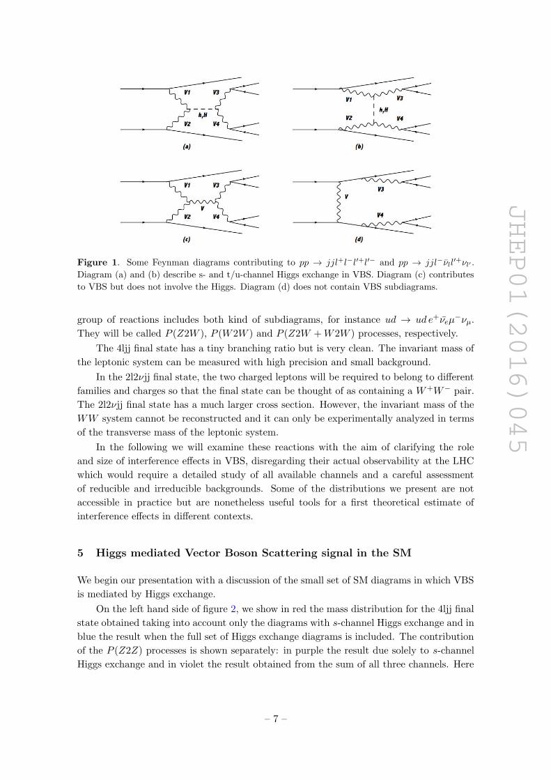
Figure 1. Some Feynman diagrams contributing to pp → jjl+l−l′+l′− and pp → jjl−νll′+νl′ .

Diagram (a) and (b) describe s- and t/u-channel Higgs exchange in VBS. Diagram (c) contributes

to VBS but does not involve the Higgs. Diagram (d) does not contain VBS subdiagrams.

group of reactions includes both kind of subdiagrams, for instance ud → ud e+νeµ−νµ.

They will be called P (Z2W ), P (W2W ) and P (Z2W +W2W ) processes, respectively.

The 4ljj final state has a tiny branching ratio but is very clean. The invariant mass of

the leptonic system can be measured with high precision and small background.

In the 2l2νjj final state, the two charged leptons will be required to belong to different

families and charges so that the final state can be thought of as containing a W+W− pair.

The 2l2νjj final state has a much larger cross section. However, the invariant mass of the

WW system cannot be reconstructed and it can only be experimentally analyzed in terms

of the transverse mass of the leptonic system.

In the following we will examine these reactions with the aim of clarifying the role

and size of interference effects in VBS, disregarding their actual observability at the LHC

which would require a detailed study of all available channels and a careful assessment

of reducible and irreducible backgrounds. Some of the distributions we present are not

accessible in practice but are nonetheless useful tools for a first theoretical estimate of

interference effects in different contexts.

5 Higgs mediated Vector Boson Scattering signal in the SM

We begin our presentation with a discussion of the small set of SM diagrams in which VBS

is mediated by Higgs exchange.

On the left hand side of figure 2, we show in red the mass distribution for the 4ljj final

state obtained taking into account only the diagrams with s-channel Higgs exchange and in

blue the result when the full set of Higgs exchange diagrams is included. The contribution

of the P (Z2Z) processes is shown separately: in purple the result due solely to s-channel

Higgs exchange and in violet the result obtained from the sum of all three channels. Here

– 7 –

JHEP01(2016)045

M4l GeV

200 400 600 800 1000 1200

fb

/GeV

d Mσ

d

7−

10

6−

10

5−

10

4−

10

3−

10

hs

h

hs_Z2Z

h_Z2Z

eemumu

M2l2v GeV

200 400 600 800 1000 1200

fb

/Ge

V

dMσ

d

5−

10

4−

10

3−

10

2−

10

1−

10

1hs

h

hs_W2W

h_W2W

emuvv

Figure 2. Invariant mass distribution of the four lepton system for the 4ljj final state (left) and

the 2l2νjj final state (right) in the SM. In red and purple the mass distribution obtained taking

into account only the diagrams with s-channel Higgs exchange and in blue and violet the result

when the full set of Higgs exchange diagrams is included. On the left(right), the two contributions

of the P (Z2Z)(P (W2W )) processes is shown separately.

and in the following, for readability, we use bins of different size around the peaks and in

the off-peak regions.

On the right hand side of figure 2 we show the corresponding results for the 2l2νjj

final state. In this case, it is the contribution of the P (W2W ) processes which is shown

separately.

We see that there is a significant difference between the curves obtained considering

only s-channel Higgs exchange and those obtained from the full set of scalar exchange

diagrams. This implies a conspicuous negative interference between the Higgs exchange

diagrams in P (Z2Z) and P (W2W ) processes. This interference is so large that it signif-

icantly modifies the result obtained when all processes are summed, even though there

are reactions which contribute substantially to the total which are not affected at all by

these effects like P (W2Z) and P (Z2W ) processes and others, the P (Z2W + W2W ) and

P (Z2Z +W2Z) groups, which are affected only partially.

Large cancellations in P (Z2Z) processes are expected. On shell ZZ → ZZ scattering is

zero in the absence of the Higgs and therefore does not violate unitarity at high energy. As

a consequence the corresponding Higgs diagrams, each of which grows as the invariant mass

squared of the process, must combine in such a way that their sum is actually asymptoti-

cally finite. At large energy, the longitudinal polarization vector of a Z boson of momentum

pµ can be identified with pµ/MZ and the sum of the three Feynman diagrams describing

the scattering behaves as s2/s+t2/t+u2/u = s+t+u ≈ 0. It is however surprising that the

cancellation grows so rapidly, above threshold, with the mass of the ZZ pair and becomes

substantial already at moderate invariant masses. For MZZ = 500 GeV the square of the

three Higgs exchange diagrams is an order of magnitude smaller than the result obtained

from s-channel exchange alone. The same cancellation takes place in the amplitude of the

P (Z2Z +W2Z) processes, while the P (W2Z) sector is unaffected. In the sum of all pro-

cesses the interference decreases the SM result for s-channel Higgs exchange by about 25%.

– 8 –

JHEP01(2016)045

Interference effects are present also in P (W2W ) processes, as shown in the right hand

side of figure 2. They are less prominent than in the P (Z2Z) case. The same cancellation

takes place in the amplitude of the P (Z2W +W2W ) processes, while the P (Z2W ) sector

is unaffected. Summing all processes, the difference between the result obtained from

the single s-channel exchange diagram (red) and the full set (blue) is larger than for 4ljj

production because WW initiated scatterings are more frequent than ZZ ones for the 2l2νjj

final state. The interference decreases the SM result for s-channel Higgs exchange by about

30%. The on shell reaction W+W− →W+W− violates unitarity in a Higgsless theory when

the W ’s are longitudinally polarized. Therefore Higgs exchange diagrams are necessary to

restore unitarity and the cancellation can only be partial. There is no u-channel exchange,

so, at large energy, the sum of the two diagrams behaves as t2/t+ s2/s = t+ s ≈ −u.

These results imply that, when producing Monte Carlo templates for the analysis of off

shell Higgs production, it is mandatory to include the full set of Higgs exchange diagrams.

This is coherent with the Caola-Melnikov method which isolates all terms in the amplitude

which are proportional to the same power of the Higgs couplings. As a consequence all

Higgs exchange diagrams need to be taken as a unit, regardless of the channel in which the

exchange takes place.

QCD radiative corrections in VBF are small. They are crucial in reducing the scale

dependence of the predictions to the 5-10% level. NNLO corrections bring the uncertainty

down to about 2%. When aiming for high accuracy, interference effects, which have a

comparable if not larger impact, cannot be ignored.

6 Higgs mediated Vector Boson Scattering signal in the 1HSM

We now turn to the 1HSM. In this case there are two sets of Higgs exchange diagrams, one

for each of the two Higgs fields in the model. In general, an amplitude involving a single

Higgs exchange can be written schematically as

A = AsP (s) +AtP (t) +AuP (u) +A0 (6.1)

where A0 does not involve the scalar fields and

P (x) =

(c2α

x−M2h + iΓhMh

+s2α

x−M2H + iΓHMH

)(6.2)

The real parts of the two terms in P (s) interfere destructively for M2h < q2 < M2

H and

constructively for q2 < M2h and M2

H < q2. In the region around s = M2h the heavy Higgs

amplitude becomes as large or larger than the light Higgs one and the interference can

be substantial. In P (t) and P (u) the two terms always have the same sign. Moreover,

the heavy Higgs amplitude will be decreased in comparison with the light Higgs one by

the larger value of the mass. As a consequence, while technically interference effects are

present in these subamplitudes, they are expected to be much less significant. Only at

large energies the masses can be neglected and the sum of the two contributions reproduce

the SM result in each channel, as required by unitarity.

– 9 –

JHEP01(2016)045

M4l GeV

200 400 600 800 1000 1200

fb

/Ge

Vd

Mσd

7−

10

6−

10

5−

10

4−

10

3−

10

hHs

hH

hHs_Z2Z

hH_Z2Z

eemumu

M2l2v GeV

200 400 600 800 1000 1200

fb

/GeV

d Mσ

d

5−

10

4−

10

3−

10

2−

10

1−

10

1hHs

hH

hHs_W2W

hH_W2W

emuvv

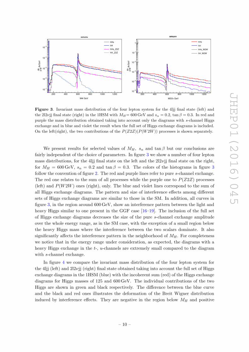
Figure 3. Invariant mass distribution of the four lepton system for the 4ljj final state (left) and

the 2l2νjj final state (right) in the 1HSM with MH= 600 GeV and sα = 0.2, tanβ = 0.3. In red and

purple the mass distribution obtained taking into account only the diagrams with s-channel Higgs

exchange and in blue and violet the result when the full set of Higgs exchange diagrams is included.

On the left(right), the two contributions of the P (Z2Z)(P (W2W )) processes is shown separately.

We present results for selected values of MH , sα and tanβ but our conclusions are

fairly independent of the choice of parameters. In figure 3 we show a number of four lepton

mass distributions, for the 4ljj final state on the left and the 2l2νjj final state on the right,

for MH = 600 GeV, sα = 0.2 and tanβ = 0.3. The colors of the histograms in figure 3

follow the convention of figure 2. The red and purple lines refer to pure s-channel exchange.

The red one relates to the sum of all processes while the purple one to P (Z2Z) processes

(left) and P (W2W ) ones (right), only. The blue and violet lines correspond to the sum of

all Higgs exchange diagrams. The pattern and size of interference effects among different

sets of Higgs exchange diagrams are similar to those in the SM. In addition, all curves in

figure 3, in the region around 600 GeV, show an interference pattern between the light and

heavy Higgs similar to one present in the GGF case [16–19]. The inclusion of the full set

of Higgs exchange diagrams decreases the size of the pure s-channel exchange amplitude

over the whole energy range, as in the SM case, with the exception of a small region below

the heavy Higgs mass where the interference between the two scalars dominate. It also

significantly affects the interference pattern in the neighborhood of MH . For completeness

we notice that in the energy range under consideration, as expected, the diagrams with a

heavy Higgs exchange in the t-, u-channels are extremely small compared to the diagram

with s-channel exchange.

In figure 4 we compare the invariant mass distribution of the four lepton system for

the 4ljj (left) and 2l2νjj (right) final state obtained taking into account the full set of Higgs

exchange diagrams in the 1HSM (blue) with the incoherent sum (red) of the Higgs exchange

diagrams for Higgs masses of 125 and 600 GeV. The individual contributions of the two

Higgs are shown in green and black respectively. The difference between the blue curve

and the black and red ones illustrates the deformation of the Breit Wigner distribution

induced by interference effects. They are negative in the region below MH and positive

– 10 –

JHEP01(2016)045

M4l GeV

200 400 600 800 1000 1200 1400

fb

/Ge

Vd

Mσd

7−

10

6−

10

5−

10

4−

10

3−

10

hH

h

H

h+H

eemumu

M2l2v GeV

200 400 600 800 1000 1200 1400

fb

/Ge

Vd

Mσd

5−

10

4−

10

3−

10

2−

10

1−

10

1hH

h

H

h+H

emuvv

Figure 4. Invariant mass distribution of the four lepton system for the 4ljj final state in the 1HSM

with MH= 600 GeV and sα = 0.2, tanβ = 0.3. In green and black the mass distribution obtained

taking into account the full set of Higgs exchange diagrams for Higgs masses of 125 and 600 GeV

respectively. In red the incoherent sum of the two contributions. In blue the result of all Higgs

diagrams in the 1HSM.

above the heavy Higgs resonance as demonstrated by the comparison of the blue and red

histograms. Effects are even larger if only the s-channel exchange is taken into account but

from now on we only consider the full set of Higgs exchange diagrams which, even though

not gauge invariant and therefore not physically observable, provides a better description

of the Higgs contribution in the off shell region.

Clearly, this interference between different Higgs fields is not a peculiarity of the Singlet

Model. It will indeed occur in any theory with multiple scalars which couple to the same

set of elementary particles, albeit possibly with different strengths.

7 Full processes

After our presentation of the interplay of the different sets of Higgs exchange diagrams,

we move to the discussion of the actual cross section for the production of a Singlet Model

heavy Higgs at the LHC. The plot on the left hand side of figure 5 shows the prediction

for 4ljj production in the 1HSM (blue) with MH= 600 GeV and sα = 0.2. Charged leptons

satisfy the requirements in eq. (4.1) while jets pass the cuts in eq. (4.2). The 1HSM exact

result, in blue, is compared with different approximations. The green histograms is the

light Higgs plus no-Higgs contribution, dσBh/dM ; the red one refers to dσBH/dM ; the gray

one to dσB/dM + dσH/dM and the brown one to dσB/dM + dσh/dM + dσH/dM . On the

right hand side of figure 5 the corresponding curves for the 2l2νjj final state are displayed.

None of the approximations in figure 5 approaches the exact result better than about 20%

in the region around the heavy scalar peak and they obviously fare even worse at large M4l,

with the exception of the green curve which misses only the heavy Higgs subamplitude,

which is proportional to s2α and numerically small in this energy range and outside the

peak region, though necessary for unitarity. Clearly, neglecting any part of an amplitude

requires a great deal of attention and a careful estimate of the resulting discrepancy.

– 11 –

JHEP01(2016)045

M4l GeV

200 300 400 500 600 700 800 900 1000

fb/G

eV

d

Mσd

5−

10

4−

10

1HSM

hB

HB

H+B

h+H+B

eemumu

M2l2v GeV

400 450 500 550 600 650 700 750 800 850

fb

/GeV

d Mσ

d

2−

10

1HSM

hB

HB

H+B

h+H+B

emuvv

Figure 5. In blue, the invariant mass distribution of the four lepton system for the 4ljj final state

(left) and the 2l2νjj final state (right) in the 1HSM with MH= 600 GeV and sα = 0.2. The other

curves are different approximations as detailed in the main text.

M4l GeV

200 300 400 500 600 700 800 900 1000

fb

/Ge

Vd

Mσd

5−

10

4−

10

3−

10

1HSM

hB+H

1HSM+qcd

eemumu

M2l2v GeV

200 300 400 500 600 700 800 900 1000

fb

/Ge

Vd

Mσd

3−

10

2−

10

1−

10

11HSM

hB+H

1HSM+qcd

emuvv

Figure 6. Invariant mass distribution of the four lepton system for the 4ljj final state (left) and

the 2l2νjj final state (right) in the 1HSM with MH= 600 GeV and sα = 0.2. The blue histogram is

the exact 1HSM result. The green line refers to dσBh/dM + dσH/dM . The red curve is the sum of

the 1HSM result and of the QCD contribution at O(α4EMα

2S).

There is however a combination of subamplitudes which provides a good approximation

to the exact result. In figure 6 the prediction for 4ljj/2l2νjj production in the 1HSM, in blue,

is compared with the curve, in green, obtained from the incoherent sum of dσBh/dM and

dσH/dM , both of them computed with 1HSM couplings and widths. The two histograms

agree remarkably well over the full mass range. This is particularly meaningful in the

region of the heavy Higgs peak where AH is large: it implies that the interference terms

of the heavy Higgs diagrams with Ah and AB cancel each other to a large degree. For

comparison, we also show in red the sum of the full O(α6EM) result discussed above and of

the QCD contribution at O(α4EMα

2S). The cross section is a factor of about three larger

than the EW result.

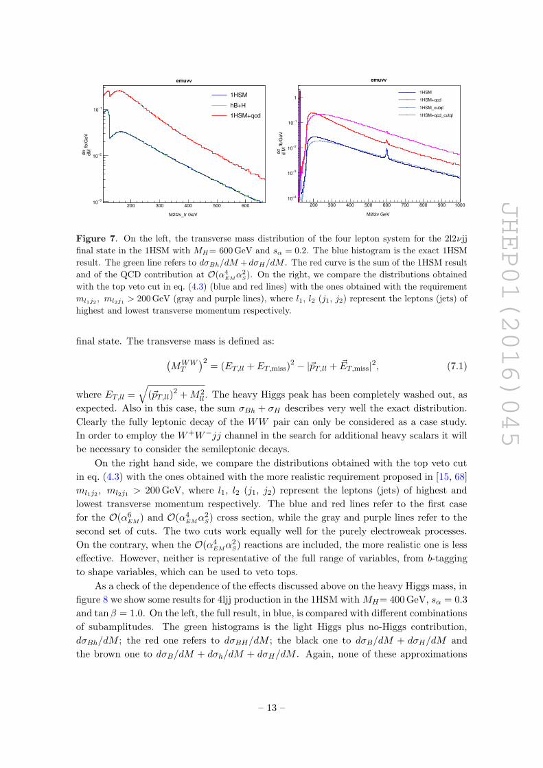
As mentioned before, the invariant mass of the W boson pair is not measurable, there-

fore on the left hand side of figure 7 we show the transverse mass distribution for the 2l2νjj

– 12 –

JHEP01(2016)045

M2l2v_tr GeV

200 300 400 500 600

fb/G

eV

d

Mσd

3−

10

2−

10

1−

10

1HSM

hB+H

1HSM+qcd

emuvv

M2l2v GeV

200 300 400 500 600 700 800 900 1000

fb

/GeV

d Mσ

d

4−

10

3−

10

2−

10

1−

10

11HSM

1HSM+qcd

1HSM_cutql

1HSM+qcd_cutql

emuvv

Figure 7. On the left, the transverse mass distribution of the four lepton system for the 2l2νjj

final state in the 1HSM with MH= 600 GeV and sα = 0.2. The blue histogram is the exact 1HSM

result. The green line refers to dσBh/dM + dσH/dM . The red curve is the sum of the 1HSM result

and of the QCD contribution at O(α4EMα

2S). On the right, we compare the distributions obtained

with the top veto cut in eq. (4.3) (blue and red lines) with the ones obtained with the requirement

ml1j2 , ml2j1 > 200 GeV (gray and purple lines), where l1, l2 (j1, j2) represent the leptons (jets) of

highest and lowest transverse momentum respectively.

final state. The transverse mass is defined as:(MWWT

)2= (ET,ll + ET,miss)

2 − |~pT,ll + ~ET,miss|2, (7.1)

where ET,ll =√

(~pT,ll)2 +M2

ll. The heavy Higgs peak has been completely washed out, as

expected. Also in this case, the sum σBh + σH describes very well the exact distribution.

Clearly the fully leptonic decay of the WW pair can only be considered as a case study.

In order to employ the W+W−jj channel in the search for additional heavy scalars it will

be necessary to consider the semileptonic decays.

On the right hand side, we compare the distributions obtained with the top veto cut

in eq. (4.3) with the ones obtained with the more realistic requirement proposed in [15, 68]

ml1j2 , ml2j1 > 200 GeV, where l1, l2 (j1, j2) represent the leptons (jets) of highest and

lowest transverse momentum respectively. The blue and red lines refer to the first case

for the O(α6EM) and O(α4

EMα2S) cross section, while the gray and purple lines refer to the

second set of cuts. The two cuts work equally well for the purely electroweak processes.

On the contrary, when the O(α4EMα

2S) reactions are included, the more realistic one is less

effective. However, neither is representative of the full range of variables, from b-tagging

to shape variables, which can be used to veto tops.

As a check of the dependence of the effects discussed above on the heavy Higgs mass, in

figure 8 we show some results for 4ljj production in the 1HSM with MH= 400 GeV, sα = 0.3

and tanβ = 1.0. On the left, the full result, in blue, is compared with different combinations

of subamplitudes. The green histograms is the light Higgs plus no-Higgs contribution,

dσBh/dM ; the red one refers to dσBH/dM ; the black one to dσB/dM + dσH/dM and

the brown one to dσB/dM + dσh/dM + dσH/dM . Again, none of these approximations

– 13 –

JHEP01(2016)045

M4l GeV

200 300 400 500 600 700

fb

/Ge

Vd

Mσd

4−

10

3−

10

1HSM

hB

HB

H+B

h+H+B

eemumu

M4l GeV

200 300 400 500 600 700 800

fb

/Ge

Vd Mσ

d

5−

10

4−

10

3−

10

1HSM

hB+H

1HSM+qcd

eemumu

Figure 8. Invariant mass distribution of the four lepton system for the 4ljj final state in the 1HSM

with MH= 400 GeV, sα = 0.3 and tanβ = 1.0. On the left, the 1HSM result, in blue, is compared

with different approximations as detailed in the main text. On the right the exact result is compared

with dσBh/dM + dσH/dM ,in green. The red curve is the sum of the 1HSM result and of the QCD

contribution at O(α4EMα

2S).

200 GeV < M4l < 1 TeV |M4l −MH | < 25 GeV

MH (GeV), sα σ σBh σBh+σH σSM σ σBh σBh+σH σSM

400, 0.3, 4l 91.2 81.2 91.3 80.8 17.0 7.5 17.0 7.5

600, 0.2, 4l 83.1 80.8 83.2 80.8 4.8 2.6 4.8 2.7

600, 0.2, 2l2ν 5565 5510 5567 5509 229 177 230 177

Table 1. Cross sections in attobarns at the LHC with a center of mass energy of 13 TeV. σ refers

to the full 1HSM result, while σSM corresponds to sα = 0. The SM cross section in |M4l −MH | <25 GeV can be considered as the SM background to the heavy Higgs.

describe satisfactorily the region around the heavy scalar peak. All of them, with the

exception of the green curve, lack terms which are crucial for the restoration of unitarity,

and progressively diverge from the exact result as the four lepton mass increases. On the

right the exact result is compared with dσBh/dM + dσH/dM . The agreement between the

two curves is impressive. In red we show the sum of the full O(α6EM) result and of the QCD

contribution at O(α4EMα

2S).

In table 1 we show the cross section in attobarns for two mass intervals: 200 GeV

< M4l < 1 TeV, which roughly coincides with the range employed so far by the experimental

collaborations to set limits on the presence and couplings of additional scalars, and |M4l−MH | < 25 GeV, as an indication of the possible effects on an analysis in smaller mass bins

which requires high luminosity. σ refers to the full 1HSM result, while σSM corresponds to

sα = 0.

We notice that σBh ≈ σSM(sα = 0) in both intervals. The only difference between the

two results is that in the first case the light Higgs couplings are scaled by cα. Therefore,

the off shell predictions are hardly affected by this modification.

The incoherent sum σBh+σH agrees with the exact result in all cases also when inte-

grated over.

– 14 –

JHEP01(2016)045

M4l GeV

500 520 540 560 580 600 620 640 660 680 700

fb/G

eV

dMσ

d

0

0.05

0.1

0.15

0.2

0.25

3−

10×

H

H+iHh

H+iHh+iHnoh

eemumu

fb

/Ge

V

dMσ

d

0.04−

0.02−

0

0.02

0.04

3−

10×

int_H_h

int_H_nohig

sum2int

eemumu

M4l GeV

560 580 600 620 640

2(I

H0

+IH

h)/

(IH

0-I

Hh

)

0.02−

0

0.02

0.04

M2l2v GeV

700 800 900 1000 1100 1200 1300 1400

fb/G

eV

dMσ

d

0.1−

0

0.1

0.2

0.3

0.4

0.5

0.6

0.7

3−

10×

H

H+iHh

H+iHh+iHnoh

emuvv

fb

/Ge

V

dMσ

d

0.2−

0.1−

0

0.1

0.2

0.33−

10×

int_H_h

int_H_nohig

sum2int

emuvv

M2l2v GeV

700 800 900 1000 1100

2(I

H0

+IH

h)/

(IH

0-I

Hh

)

0

0.1

0.2

Figure 9. In the upper row, the invariant mass distribution of the four lepton system for the 4l

final state in the 1HSM with MH= 600 GeV and sα = 0.2. In the lower row the corresponding plots

for the 2l2νjj final state with MH= 900 GeV and sα = 0.4. On the left we show dσH/dM (blue),

dσH/dM + dIhH/dM (red) and dσH/dM + dIhH/dM + dIBH/dM (green). On the right we show

dIhH/dM (red), dIBH/dM (violet) and dIhH/dM + dIBH/dM (green).

The predicted number of heavy Higgs events at the LHC in the three cases detailed in

table 1, taking into account an additional factor of two when summing over all combinations

of light leptons, is 6/1/18 for the expected luminosity of 300 fb−1 in Run II. The signal to

background ratio is of order one. Detecting a 1HSM heavy Higgs in VBF at the LHC will

be challenging, even after the high luminosity upgrade.

8 Cancellation of the heavy Higgs interferences

It is noteworthy that the interference terms of the heavy Higgs diagrams with Ah and ABcancel each other almost exactly for different ranges of invariant mass of the final state

vector boson pair and different small amounts of mixing between the light and heavy Higgs.

The interference corresponds to the integral of

I = 2< (A∗H × (AB +Ah)) = 2<(A∗H ×

(AB + c2

αASMh

)). (8.1)

Since Ah ∝ c2α, the cancellation cannot take place for arbitrary values of the mixing angle α.

– 15 –

JHEP01(2016)045

In order to investigate further this phenomenon, in figure 9 we isolate the interference

terms for different choices of parameters. In the upper row, we show the invariant mass

distribution of the four lepton system for the 4l final state in the 1HSM with MH= 600 GeV

and sα = 0.2. In the lower row the corresponding plots for the 2l2νjj final state is given

with MH= 900 GeV and sα = 0.4, a rather extreme case in view of the allowed parameter

space. Defining Iij as the integrated interference between Ai and Aj , on the right we show

dσhH/dM − dσh/dM − dσH/dM = dIhH/dM (red), dσHB/dM − dσB/dM − dσH/dM =

dIBH/dM (violet) and dIhH/dM + dIBH/dM (green). On the left we show dσH/dM in

blue, dσH/dM + dIhH/dM (red) and dσH/dM + dIhH/dM + dIBH/dM (green).

The plot in the upper left corner shows how, for MH= 600 GeV and sα = 0.2, the

interference between the heavy and the light Higgs deforms the Breit-Wigner distribution

of the heavy scalar and how the inclusion of the interference between the heavy Higgs and

the subamplitude without any Higgs practically eliminates the deformation. The plot on

the top right displays the two interferences and their sum, which is much smaller. The

red and violet continuous lines are fits to the corresponding histograms with functions of

the form:

f = AM2V V −M2

H(M2V V −M2

H

)2+ Γ2

HM2H

+B(M2V V −M2

H

)C(8.2)

where A, B and C are free parameters. The green continuous line is the sum of the red

and violet ones. The lower subplot shows the ratio

R = 2dIBH/dM + dIhH/dM

dIBH/dM − dIhH/dM, (8.3)

where the fitting functions have been used in place of the actual histograms in order to

smooth out the oscillations. Notice that in the ratio the common factor s2α cancels, there-

fore, the degree of cancellation between the two terms does not depend on the smallness

of the heavy Higgs couplings.

In the region of the heavy resonance R is about 4% .

The two plots in the lower part provide the same information for the 2l2νjj final state

with MH= 900 GeV and sα = 0.4. Since now s2α = 0.16 is larger than in the previous

example, the interference between the heavy scalar and the noHiggs amplitude is larger in

absolute value than the interference between the two Higgs. As a consequence the sum is

clearly non zero and agrees in sign with the former of the two interferences. In the region

of the heavy resonance R is about 20%.

In order to appreciate these results, it is useful to compare them with the correspond-

ing values for the gg → V V → 4l, 2l2ν case, which can be extracted from table 6 and

table 8 of ref. [18]. Under the reasonable assumption that the light Higgs and background

amplitudes vary little within one heavy Higgs width around the peak, the ratio of inte-

grated interferences reproduce the ratio of amplitudes which define R, eq. (8.3). For the

gg → ZZ → 4l, with MH= 600 GeV and sα = sin(π/15) = 0.208, one finds R = 1.78. For

the gg →W+W− → 2l2ν, with MH= 900 GeV and sα = sin(π/8) = 0.383, R = 1.49.

The vector bosons in the heavy Higgs decay, for all the masses we have considered,

are predominantly longitudinally polarized. Unitarity requires that the leading term of the

– 16 –

JHEP01(2016)045

contributions to jjVLVL production from vector boson interactions and the contribution

from all Higgs exchanges must cancel each other exactly in the large energy limit, where

vector and Higgs masses can be neglected. Subleading terms are not affected and therefore

jjVLVL production is not necessarily zero. The near perfect suppression we observe between

AB and Ah, which results in a small interference of the heavy Higgs with the rest of the

amplitude, suggests that the cancellation between AB and Ah sets in already for invariant

masses of the vector pair of a few hundred GeV, provided the mixing angle is not too large,

an energy much smaller than the scale at which on shell VLVL scattering violates unitarity

in a Higgsless theory.

From eq. (8.3) and eq. (8.1) one can extract the ratio of the two interferences, Rh/B

Rh/B =dIhH/dM

dIBH/dM= c2

α

dISMhH /dM

dIBH/dM= c2

αR0h/B = −1−R/2

1 +R/2. (8.4)

For MH= 600 GeV and sα = 0.2, Rh/B = −0.961, while for MH = 900 GeV and sα = 0.4,

Rh/B = −0.818. Eq. (8.4) shows that, as the mixing angle α approaches zero, the ratio

between the two interference terms approaches minus one. In fact, the values for R0h/B

in the two cases examined are −1.001 and −0.974, respectively. In this limit, the heavy

Higgs exchange amplitude is probing the cancellation between the Standard Model Higgs

exchange and background amplitudes, which appears to be at the percent level.

9 Conclusions

We have studied Higgs sector interference effects in Vector Boson Scattering at the LHC,

both in the Standard Model and its one Higgs Singlet extension as a prototype of theories

in which more than one neutral, CP even, scalars are present. We have concentrated

on pp → jj l+l−l′+l′− and pp → jj l−νll′+νl′ production. We have shown that large

interferences among the different Higgs exchange channels are present in the SM and that

a production times decay approach fails to reproduce the off shell Higgs contribution.

In the 1HSM, there are additional interferences between the two Higgs fields. Different

approximations have been tried and proved inaccurate. We have found that the interference

between the heavy Higgs diagrams and the rest of the amplitude, which is the sum of light

Higgs exchange diagrams and of those diagrams in which no Higgs appear, is very small

for values of the mixing angle compatible with the experimental constraints and can be

neglected.

Acknowledgments

Several stimulating discussions with Anna Kropivnitskaya and Pietro Govoni are grate-

fully acknowledged. This work has been supported by MIUR (Italy) under contract

2010YJ2NYW 006, by the Compagnia di San Paolo under contract ORTO11TPXK and

by the European Union Initial Training Network HiggsTools (PITN-GA-2012-316704).

Open Access. This article is distributed under the terms of the Creative Commons

Attribution License (CC-BY 4.0), which permits any use, distribution and reproduction in

any medium, provided the original author(s) and source are credited.

– 17 –

JHEP01(2016)045

References

[1] ATLAS collaboration, Observation of a new particle in the search for the Standard Model

Higgs boson with the ATLAS detector at the LHC, Phys. Lett. B 716 (2012) 1

[arXiv:1207.7214] [INSPIRE].

[2] CMS collaboration, Observation of a new boson at a mass of 125 GeV with the CMS

experiment at the LHC, Phys. Lett. B 716 (2012) 30 [arXiv:1207.7235] [INSPIRE].

[3] CMS collaboration, Precise determination of the mass of the Higgs boson and tests of

compatibility of its couplings with the standard model predictions using proton collisions at 7

and 8 TeV, Eur. Phys. J. C 75 (2015) 212 [arXiv:1412.8662] [INSPIRE].

[4] ATLAS, CMS collaborations, Combined Measurement of the Higgs Boson Mass in pp

Collisions at√s = 7 and 8 TeV with the ATLAS and CMS Experiments, Phys. Rev. Lett.

114 (2015) 191803 [arXiv:1503.07589] [INSPIRE].

[5] ATLAS collaboration, Updated coupling measurements of the Higgs boson with the ATLAS

detector using up to 25 fb−1 of proton-proton collision data, ATLAS-CONF-2014-009 (2014).

[6] ATLAS collaboration, Constraints on New Phenomena via Higgs Coupling Measurements

with the ATLAS Detector, ATLAS-CONF-2014-010 (2014).

[7] CMS collaboration, Searches for new processes in the scalar sector at the CMS experiment,

PoS(DIS2014)109 [INSPIRE].

[8] N. Kauer and G. Passarino, Inadequacy of zero-width approximation for a light Higgs boson

signal, JHEP 08 (2012) 116 [arXiv:1206.4803] [INSPIRE].

[9] F. Caola and K. Melnikov, Constraining the Higgs boson width with ZZ production at the

LHC, Phys. Rev. D 88 (2013) 054024 [arXiv:1307.4935] [INSPIRE].

[10] J.M. Campbell, R.K. Ellis and C. Williams, Bounding the Higgs width at the LHC using full

analytic results for gg → e−e+µ−µ+, JHEP 04 (2014) 060 [arXiv:1311.3589] [INSPIRE].

[11] J.M. Campbell, R.K. Ellis and C. Williams, Bounding the Higgs width at the LHC:

Complementary results from H →WW , Phys. Rev. D 89 (2014) 053011 [arXiv:1312.1628]

[INSPIRE].

[12] CMS collaboration, Constraints on the Higgs boson width from off-shell production and

decay to Z-boson pairs, Phys. Lett. B 736 (2014) 64 [arXiv:1405.3455] [INSPIRE].

[13] ATLAS collaboration, Constraints on the off-shell Higgs boson signal strength in the

high-mass ZZ and WW final states with the ATLAS detector, Eur. Phys. J. C 75 (2015)

335 [arXiv:1503.01060] [INSPIRE].

[14] CMS collaboration, Limits on the Higgs boson lifetime and width from its decay to four

charged leptons, Phys. Rev. D 92 (2015) 072010 [arXiv:1507.06656] [INSPIRE].

[15] J.M. Campbell and R.K. Ellis, Higgs Constraints from Vector Boson Fusion and Scattering,

JHEP 04 (2015) 030 [arXiv:1502.02990] [INSPIRE].

[16] C. Englert, Y. Soreq and M. Spannowsky, Off-Shell Higgs Coupling Measurements in BSM

scenarios, JHEP 05 (2015) 145 [arXiv:1410.5440] [INSPIRE].

[17] E. Maina, Interference effects in Heavy Higgs production via gluon fusion in the Singlet

Extension of the Standard Model, JHEP 06 (2015) 004 [arXiv:1501.02139] [INSPIRE].

– 18 –

JHEP01(2016)045

[18] N. Kauer and C. O’Brien, Heavy Higgs signal-background interference in gg → V V in the

Standard Model plus real singlet, Eur. Phys. J. C 75 (2015) 374 [arXiv:1502.04113]

[INSPIRE].

[19] C. Englert, I. Low and M. Spannowsky, On-shell interference effects in Higgs boson final

states, Phys. Rev. D 91 (2015) 074029 [arXiv:1502.04678] [INSPIRE].

[20] C. Englert and M. Spannowsky, Limitations and Opportunities of Off-Shell Coupling

Measurements, Phys. Rev. D 90 (2014) 053003 [arXiv:1405.0285] [INSPIRE].

[21] V. Silveira and A. Zee, Scalar phantoms, Phys. Lett. B 161 (1985) 136 [INSPIRE].

[22] R. Schabinger and J.D. Wells, A Minimal spontaneously broken hidden sector and its impact

on Higgs boson physics at the large hadron collider, Phys. Rev. D 72 (2005) 093007

[hep-ph/0509209] [INSPIRE].

[23] D. O’Connell, M.J. Ramsey-Musolf and M.B. Wise, Minimal Extension of the Standard

Model Scalar Sector, Phys. Rev. D 75 (2007) 037701 [hep-ph/0611014] [INSPIRE].

[24] O. Bahat-Treidel, Y. Grossman and Y. Rozen, Hiding the Higgs at the LHC, JHEP 05

(2007) 022 [hep-ph/0611162] [INSPIRE].

[25] V. Barger, P. Langacker, M. McCaskey, M.J. Ramsey-Musolf and G. Shaughnessy, LHC

Phenomenology of an Extended Standard Model with a Real Scalar Singlet, Phys. Rev. D 77

(2008) 035005 [arXiv:0706.4311] [INSPIRE].

[26] G. Bhattacharyya, G.C. Branco and S. Nandi, Universal Doublet-Singlet Higgs Couplings

and phenomenology at the CERN Large Hadron Collider, Phys. Rev. D 77 (2008) 117701

[arXiv:0712.2693] [INSPIRE].

[27] M. Gonderinger, Y. Li, H. Patel and M.J. Ramsey-Musolf, Vacuum Stability, Perturbativity

and Scalar Singlet Dark Matter, JHEP 01 (2010) 053 [arXiv:0910.3167] [INSPIRE].

[28] S. Dawson and W. Yan, Hiding the Higgs Boson with Multiple Scalars, Phys. Rev. D 79

(2009) 095002 [arXiv:0904.2005] [INSPIRE].

[29] S. Bock, R. Lafaye, T. Plehn, M. Rauch, D. Zerwas and P.M. Zerwas, Measuring Hidden

Higgs and Strongly-Interacting Higgs Scenarios, Phys. Lett. B 694 (2011) 44

[arXiv:1007.2645] [INSPIRE].

[30] P.J. Fox, D. Tucker-Smith and N. Weiner, Higgs friends and counterfeits at hadron colliders,

JHEP 06 (2011) 127 [arXiv:1104.5450] [INSPIRE].

[31] C. Englert, T. Plehn, D. Zerwas and P.M. Zerwas, Exploring the Higgs portal, Phys. Lett. B

703 (2011) 298 [arXiv:1106.3097] [INSPIRE].

[32] C. Englert, J. Jaeckel, E. Re and M. Spannowsky, Evasive Higgs Maneuvers at the LHC,

Phys. Rev. D 85 (2012) 035008 [arXiv:1111.1719] [INSPIRE].

[33] B. Batell, S. Gori and L.-T. Wang, Exploring the Higgs Portal with 10/fb at the LHC, JHEP

06 (2012) 172 [arXiv:1112.5180] [INSPIRE].

[34] C. Englert, T. Plehn, M. Rauch, D. Zerwas and P.M. Zerwas, LHC: Standard Higgs and

Hidden Higgs, Phys. Lett. B 707 (2012) 512 [arXiv:1112.3007] [INSPIRE].

[35] R.S. Gupta and J.D. Wells, Higgs boson search significance deformations due to mixed-in

scalars, Phys. Lett. B 710 (2012) 154 [arXiv:1110.0824] [INSPIRE].

[36] B. Batell, D. McKeen and M. Pospelov, Singlet Neighbors of the Higgs Boson, JHEP 10

(2012) 104 [arXiv:1207.6252] [INSPIRE].

– 19 –

JHEP01(2016)045

[37] D. Bertolini and M. McCullough, The Social Higgs, JHEP 12 (2012) 118 [arXiv:1207.4209]

[INSPIRE].

[38] J.M. No and M. Ramsey-Musolf, Probing the Higgs Portal at the LHC Through Resonant

di-Higgs Production, Phys. Rev. D 89 (2014) 095031 [arXiv:1310.6035] [INSPIRE].

[39] G.M. Pruna and T. Robens, Higgs singlet extension parameter space in the light of the LHC

discovery, Phys. Rev. D 88 (2013) 115012 [arXiv:1303.1150] [INSPIRE].

[40] D. Lopez-Val and T. Robens, ∆r and the W-boson mass in the singlet extension of the

standard model, Phys. Rev. D 90 (2014) 114018 [arXiv:1406.1043] [INSPIRE].

[41] S. Profumo, M.J. Ramsey-Musolf, C.L. Wainwright and P. Winslow, Singlet-catalyzed

electroweak phase transitions and precision Higgs boson studies, Phys. Rev. D 91 (2015)

035018 [arXiv:1407.5342] [INSPIRE].

[42] C.-Y. Chen, S. Dawson and I.M. Lewis, Exploring resonant di-Higgs boson production in the

Higgs singlet model, Phys. Rev. D 91 (2015) 035015 [arXiv:1410.5488] [INSPIRE].

[43] T. Robens and T. Stefaniak, Status of the Higgs Singlet Extension of the Standard Model

after LHC Run 1, Eur. Phys. J. C 75 (2015) 104 [arXiv:1501.02234] [INSPIRE].

[44] H.E. Logan, Hiding a Higgs width enhancement from off-shell gg(→ h∗)→ ZZ

measurements, Phys. Rev. D 92 (2015) 075038 [arXiv:1412.7577] [INSPIRE].

[45] V. Martın Lozano, J.M. Moreno and C.B. Park, Resonant Higgs boson pair production in the

hh→ bb WW → bb`+ν`−ν decay channel, JHEP 08 (2015) 004 [arXiv:1501.03799]

[INSPIRE].

[46] A. Falkowski, C. Gross and O. Lebedev, A second Higgs from the Higgs portal, JHEP 05

(2015) 057 [arXiv:1502.01361] [INSPIRE].

[47] M. Ciccolini, A. Denner and S. Dittmaier, Strong and electroweak corrections to the

production of Higgs + 2jets via weak interactions at the LHC, Phys. Rev. Lett. 99 (2007)

161803 [arXiv:0707.0381] [INSPIRE].

[48] M. Ciccolini, A. Denner and S. Dittmaier, Electroweak and QCD corrections to Higgs

production via vector-boson fusion at the LHC, Phys. Rev. D 77 (2008) 013002

[arXiv:0710.4749] [INSPIRE].

[49] B. Jager, C. Oleari and D. Zeppenfeld, Next-to-leading order QCD corrections to W+W-

production via vector-boson fusion, JHEP 07 (2006) 015 [hep-ph/0603177] [INSPIRE].

[50] B. Jager, C. Oleari and D. Zeppenfeld, Next-to-leading order QCD corrections to Z boson

pair production via vector-boson fusion, Phys. Rev. D 73 (2006) 113006 [hep-ph/0604200]

[INSPIRE].

[51] B. Jager, C. Oleari and D. Zeppenfeld, Next-to-leading order QCD corrections to W+ W+ jj

and W- W- jj production via weak-boson fusion, Phys. Rev. D 80 (2009) 034022

[arXiv:0907.0580] [INSPIRE].

[52] P. Bolzoni, F. Maltoni, S.-O. Moch and M. Zaro, Higgs production via vector-boson fusion at

NNLO in QCD, Phys. Rev. Lett. 105 (2010) 011801 [arXiv:1003.4451] [INSPIRE].

[53] P. Bolzoni, F. Maltoni, S.-O. Moch and M. Zaro, Vector boson fusion at NNLO in QCD: SM

Higgs and beyond, Phys. Rev. D 85 (2012) 035002 [arXiv:1109.3717] [INSPIRE].

[54] M. Cacciari, F.A. Dreyer, A. Karlberg, G.P. Salam and G. Zanderighi, Fully Differential

Vector-Boson-Fusion Higgs Production at Next-to-Next-to-Leading Order, Phys. Rev. Lett.

115 (2015) 082002 [arXiv:1506.02660] [INSPIRE].

– 20 –

JHEP01(2016)045

[55] A. Ballestrero, A. Belhouari, G. Bevilacqua, V. Kashkan and E. Maina, PHANTOM: A

Monte Carlo event generator for six parton final states at high energy colliders, Comput.

Phys. Commun. 180 (2009) 401 [arXiv:0801.3359] [INSPIRE].

[56] A. Ballestrero, D.B. Franzosi and E. Maina, Vector-Vector scattering at the LHC with two

charged leptons and two neutrinos in the final state, JHEP 06 (2011) 013 [arXiv:1011.1514]

[INSPIRE].

[57] N.D. Christensen and C. Duhr, FeynRules — Feynman rules made easy, Comput. Phys.

Commun. 180 (2009) 1614 [arXiv:0806.4194] [INSPIRE].

[58] A. Alloul, N.D. Christensen, C. Degrande, C. Duhr and B. Fuks, FeynRules 2.0 — A

complete toolbox for tree-level phenomenology, Comput. Phys. Commun. 185 (2014) 2250

[arXiv:1310.1921] [INSPIRE].

[59] C. Degrande, C. Duhr, B. Fuks, D. Grellscheid, O. Mattelaer and T. Reiter, UFO — The

Universal FeynRules Output, Comput. Phys. Commun. 183 (2012) 1201 [arXiv:1108.2040]

[INSPIRE].

[60] Ya. B. Zeldovich, I. Yu. Kobzarev and L.B. Okun, Cosmological Consequences of the

Spontaneous Breakdown of Discrete Symmetry, Zh. Eksp. Teor. Fiz. 67 (1974) 3 [INSPIRE].

[61] T.W.B. Kibble, Topology of Cosmic Domains and Strings, J. Phys. A 9 (1976) 1387

[INSPIRE].

[62] T.W.B. Kibble, Some Implications of a Cosmological Phase Transition, Phys. Rept. 67

(1980) 183 [INSPIRE].

[63] S.A. Abel, S. Sarkar and P.L. White, On the cosmological domain wall problem for the

minimally extended supersymmetric standard model, Nucl. Phys. B 454 (1995) 663

[hep-ph/9506359] [INSPIRE].

[64] A. Friedland, H. Murayama and M. Perelstein, Domain walls as dark energy, Phys. Rev. D

67 (2003) 043519 [astro-ph/0205520] [INSPIRE].

[65] V. Barger, P. Langacker, M. McCaskey, M. Ramsey-Musolf and G. Shaughnessy, Complex

Singlet Extension of the Standard Model, Phys. Rev. D 79 (2009) 015018 [arXiv:0811.0393]

[INSPIRE].

[66] LHC Higgs Cross Section Working Group collaboration, J.R. Andersen et al., Handbook of

LHC Higgs Cross Sections: 3. Higgs Properties, arXiv:1307.1347 [INSPIRE].

[67] J. Pumplin, D.R. Stump, J. Huston, H.L. Lai, P.M. Nadolsky and W.K. Tung, New

generation of parton distributions with uncertainties from global QCD analysis, JHEP 07

(2002) 012 [hep-ph/0201195] [INSPIRE].

[68] M. Szleper, The Higgs boson and the physics of WW scattering before and after Higgs

discovery, arXiv:1412.8367 [INSPIRE].

– 21 –