Incompressible Multiphase flow and Encapsulation

simulations using the moment of fluid method 1

Guibo Lia, Yongsheng Lianb, Yisen Guoc, Matthew Jemisond, MarkSussmane, Trevor Helmsf, Marco Arientig

aMechanical Engineering, University of Louisville, Louisville, KY, U.S.AbMechanical Engineering, University of Louisville, Louisville, KY, U.S.AcMechanical Engineering, University of Louisville, Louisville, KY, U.S.A

dMathematics, Florida State University, Tallahassee, FL, U.S.AeMathematics, Florida State University, Tallahassee, FL, U.S.AfMathematics, Florida State University, Tallahassee, FL, U.S.A

gSandia National Labs, Livermore, CA, U.S.A

Abstract

A moment of fluid method is presented for computing solutions to incom-pressible multiphase flows in which the number of materials can be greaterthan two. In this work, the multimaterial moment-of-fluid interface repre-sentation technique is applied to simulating surface tension effects at pointswhere three materials meet. The advection terms are solved using a direc-tionally split cell integrated semi-Lagrangian algorithm and the projectionmethod is used to evaluate the pressure gradient force term. The underlyingcomputational grid is a dynamic block structured adaptive grid. The newmethod is applied to multiphase problems illustrating contact line dynamics,triple junctions, and encapsulation in order to demonstrate its capabilities.Examples are given in 2D, 3D axisymmetric (R-Z), and 3D (X-Y-Z) coordi-nate systems.

Keywords: multi-phase flow, Moment of fluid method, Interface

1G. Li and Y. Lian acknowledge the support from General Electric. M. Sussman and M.Jemison acknowledge the support by the National Science Foundation under contract DMS1016381. M. Arienti acknowledges the support by Sandia National Laboratories via theLaboratory Directed Research and Development program. Sandia National Laboratoriesis a multi-program laboratory managed and operated by Sandia Corporation, a whollyowned subsidiary of Lockheed Martin Corporation, for the U. S. Department of Energy’sNational Nuclear Security Administration under contract DE-AC04-94AL85000.

Preprint submitted to International Journal for Numerical Methods in FluidsJune 22, 2015

reconstruction, Interface advection, contact line dynamics, triple junctions,gas-liquid jet flow, droplet impact, droplet collision

1. Introduction

Multiphase flow plays an important role in many technical applicationsincluding ink-jet printing, spray cooling, icing, combustion and agriculturalirrigation. The instability of the interface, mass and heat transfer acrossthe interface, and phase change make multiphase flow problems challeng-ing. Theoretical studies of multiphase flows are mainly based on linear the-ories (Rayleigh, 1878; Taylor, 1963) but yet most phenomena in multiphaseflows display nonlinear feedback mechanisms. Modern experimental studiesemploy high-speed cameras, pulsed shadowgraph, and holograph techniques(Sallam et al., 1999, 2004; Palacios et al., 2010) in order to understand thecomplex processes in multiphase flows, nonetheless, it is still very difficult tocapture the detailed flow fields.

Computational fluid dynamics (CFD) has the potential to increase ones’understanding of multiphase flow phenomena by allowing one to investigateflow fields deeply embedded within materials, study the effect of random fluc-tuations, and allowing one to precisely control initial and boundary condi-tions. Quantities such as interface surface area, streamlines, stress fields, andvorticity are easily extracted from CFD simulations. Three major challengesexist for the accurate and efficient computation of multiphase flows. First,the density and viscosity ratios between different phases can be high and itis difficult to accurately calculate the flux during the momentum advection(Raessi, 2008; Raessi and Pitsch, 2009). Second, surface tension takes effectonly at the interface between different phases and this singularity may causeproblems when solving the Navier-Stokes equations (Brackbill et al., 1992;Desjardins et al., 2008). Third, the drastic change of interface topology anddisparity in length scales make interface capturing and interface advectionchallenging (Menard et al., 2007; Li et al., 2010).

Among the different interface capturing methods, the volume-of-fluid(VOF) method (Hirt and Nichols, 1981; Brackbill et al., 1992; Pilliod Jrand Puckett, 2004) , the level set method (Osher and Sethian, 1988; Suss-man et al., 1994, 1998, 1999; Osher and Fedkiw, 2001) and their derivativesare widely used.

The VOF method tracks the volume fraction function within each com-putational grid cell. The interface is reconstructed and advected based on

2

the volume fraction function information. The benefit of VOF methods isthat there have been devised either directionally split advection algorithmsRudman (1998); Scardovelli and Zaleski (2003); Jemison et al. (2013); Wey-mouth and Yue (2010) or unsplit advection algorithms (Liovic et al., 2006;Chenadec and Pitsch, 2013; Jemison et al., 2015) which have excellent volumepreservation properties.

The level set method uses a smooth distance function to implicitly rep-resent the interface. On the one hand, the level set method is amenable tocomputing flows with surface tension effects since the distance function issmooth across the interface, on the other hand, volume conservation for thelevel set method is not guaranteed, even if the level set advection equation isdiscretized in conservation form. The coupled level set and volume-of-fluid(CLSVOF) method (Sussman and Puckett, 2000; Son and Hur, 2002; Suss-man, 2003; Menard et al., 2007; Wang et al., 2009) has also been developed.Even though the specific implementations of CLSVOF methods vary, theoverriding theme of CLSVOF methods is that they maintain the advantagesof both the level set method and the VOF method in simultaneously con-serving volume and accurately capturing the interface (Sussman and Puckett,2000; Wang et al., 2009).

Recently, the moment of fluid (MOF) method (Dyadechko and Shashkov,2005; Ahn and Shashkov, 2007; Dyadechko and Shashkov, 2008; Ahn andShashkov, 2009; Ahn et al., 2009; Jemison et al., 2013, 2014, 2015) has beendeveloped. In addition to the volume fraction function used in the VOFmethod, the MOF method considers the material centroid information inthe interface reconstruction process and can be considered a generalizationof the VOF method. The MOF interface reconstruction is completely localbecause of the introduction of centroid information. This feature enables theMOF method to capture corners and sheets significantly better than the VOFmethod for passively advected flows. Results of benchmark tests comparingMOF to VOF and CLSVOF are reported in (Kucharik et al., 2010; Wanget al., 2012; Jemison et al., 2013). A further advantage of the moment offluid representation is that the added centroid information enables the MOFmethod to straightforwardly reconstruct any number of materials, i.e. two ormore, in a given cell, conserving volume of each material (Ahn and Shashkov,2007; Jemison et al., 2015).

We remark that there have previously been developed the following VOFtriple junction reconstruction algorithms: the “onion skin” approach in whichthe materials do not intersect (Sijoy and Chaturvedi, 2010), the material or-

3

der independent weighted Voronoi diagram (also known as a power diagram)approach for 2D reconstruction of triple points applied to static configura-tions (Schofield et al., 2008), an optimization method for the localization ofthe triple point applied to 2D passive transport problems (Caboussat et al.,2008), and an improved material order independent weighted Voronoi dia-gram approach in which a novel optimization procedure was developed fordetermining interface(s) normals (Schofield et al., 2009).

We have taken the “nested dissection” MOF approach; if a computationalcell contains M materials, then there will be M − 1 linear cuts in the cell,some cuts potentially intersecting previous cuts. The MOF algorithm canreconstruct interface configurations where 3 materials meet at a single point,albeit one of the angles separating 2 of the materials must be 90 degrees.

In this paper, we describe a novel method in which we use the MOFmultimaterial reconstruction algorithm in order to simulate incompressiblemultiphase flow in two or three dimensions in which (i) two fluids with dis-parate material properties can meet at a third rigid material (contact linedynamics) and (ii) three fluids with disparate material properties meet at atriple junction. As in (Jemison et al., 2014), we maintain and update thevelocity at both cell centers and face centers. The velocity is interpolatedfrom cell centers to face centers using mass weighting where the MOF recon-struction determines the weights. Pressure is interpolated from cell centers toface centers using the condition of constant contact, where again the weightsdepend on the MOF reconstructed interface.

In what follows we describe our incompressible multi-phase MOF method,and we describe the algorithm that we have developed for the simulation ofcontact line dynamics and triple point dynamics. Example simulations aregiven with validations through grid refinement studies and comparisons withexperiments and finally conclusions are drawn.

2. Governing equations

The governing equations for incompressible, immiscible, multiphase flowsare:

∇ · u = 0 (1)

∂φm∂t

+ u · ∇φm = 0, m = 1, . . . ,M (2)

4

∂u

∂t+ u · ∇u = −∇pm

ρm+∇ · (2µmD)

ρm+ g if φm(x, t) > 0 (3)

where φm is a level set function for material m and satisfies,

φm(x, t) =

> 0 x ∈ material m≤ 0 otherwise

u = (u, v, w) is the velocity vector, t is the time, pm is the pressure for mate-rial m, g is the gravitational acceleration vector, D is the rate of deformationtensor,

D =∇u + (∇u)T

2,

and µm and ρm are the viscosity and density respectively for material m.At material interfaces, if there is no mass transfer, the velocity for all

materials are the same. For two phase flow problems (M = 2), at a materialinterface that separates material m1 from m2 (i.e. φm1(x, t) = φm2(x, t) = 0),the stress will have the following jump condition due to the effect of thesurface tension force,

((−pm1I + 2µm1D)− (−pm2I + 2µm2D)) · nm1 = σm1,m2κm1nm1

where σm1,m2 is the surface tension coefficient, the normal that points frommaterial m2 into m1 is,

nm1 =∇φm1

|∇φm1|,

and the curvature is,

κm1 = ∇ · ∇φm1

|∇φm1|.

An one-fluid formulation of (3) can be written as follows (Kim, 2007):

∂ρu

∂t+∇ · (ρu⊗ u) = −∇p+∇ · (2µD) + ρg −

M∑m=1

γmκm∇H(φm) (4)

where H(φ) is the Heaviside function defined as,

H(φ) =

1 φ ≥ 00 otherwise

, (5)

5

the combined density ρ is,

ρ =M∑m=1

ρmH(φm),

the combined viscosity, µ, is,

µ =M∑m=1

µmH(φm),

and (3 material case):

γ1 =σ12 + σ13 − σ23

2(6)

γ2 =σ12 + σ23 − σ13

2(7)

γ3 =σ13 + σ23 − σ12

2(8)

3. Numerical method

We describe our numerical method for two dimensional problems, but themethod is straightforwardly generalizable to three dimensions.

3.1. Overview of the method

The numerical method, which is based on an approximate projectionmethod (Jemison et al., 2013), is given in the following list of steps. Thespatial discretization details for each step are explained in the ensuing sec-tions.

1. At the beginning of the time step t = tn, and in each computational cell,

Ωi,j = x : xi −∆x/2 < x < xi + ∆x/2, yj −∆y/2 < y < yj + ∆y/2,

the following variables are given: mass weighted average of velocity(un

i,j), Discretely, divergence free velocity on MAC grid,

uMAC,ni+1/2,j − u

MAC,ni−1/2,j

∆x+vMAC,ni,j+1/2 − v

MAC,ni,j−1/2

∆y= 0,

volume fraction, F nm,i,j, and centroid, xnm,i,j, for each material m. Figure

1 illustrates our discretization.

6

2.Advection: Referring to (4) and (2), the directionally split cell integratedsemi-Lagrangian (CISL) method is used to solve the following equa-tions:

(ρu)t +∇ · (ρu⊗ u) = 0 (9)

(Fm)t +∇ · (uFm) = 0 (10)

The details of CISL advection are given in section 3.2.

3. Distance functions: Distance functions, φn+1m,i,j, are derived from the

non-tessellating MOF reconstructed interface for each material m =1, . . . ,M . The distance functions are used to approximate interfacecurvature. See section 3.3.

4. Viscosity, gravity, surface tension: Referring to (4),

V = uadvect + ∆t1

ρ

(∇ · (2µD) + ρg −

M∑m=1

γmκm∇H(φm)

)(11)

See sections 3.4 and 3.5.

5. Approximate projection: A variable density approximate projectionalgorithm is used to discretize the pressure gradient force,

un+1 = V −∆t∇pρ,

where p solves,

∇ · ∇pρ

=1

∆t∇ · V .

See section 3.6

6. The block structured adaptive grid is regenerated depending on the newlocations of material interfaces and then the algorithm returns back tostep 2.

7

Figure 1: The volume fractions Fm, centroids xm (filled in circles), and cellcentered velocity, u, are cell averaged quantities, and the face centered veloc-ity (filled in rectangles), uMAC , vMAC are face averaged quantities. There are3 materials illustrated in this figure. The center coordinate of the illustrated3x3 block of cells is (xi, yj).

8

3.2. Directionally Split CISL Multiphase Advection

The CISL algorithm has three parts: (i) interface reconstruction, (ii)momentum reconstruction, and (ii) mapping of reconstructed solution intocomputational cells from a given cells’ preimage.

3.2.1. Moment of Fluid Interface Reconstruction

The moment-of-fluid method(Dyadechko and Shashkov, 2005; Ahn andShashkov, 2007; Dyadechko and Shashkov, 2008; Ahn and Shashkov, 2009;Jemison et al., 2013) is used to represent material interfaces. For a compu-tational cell Ωi,j, the volume fraction (zeroth order moment) and centroid(first order moment) are:

Fm =1

|Ωi,j|

∫Ωi,j

H(φm(x))dx,

xm =

∫Ωi,j

H(φm(x))xdx∫Ωi,j

H(φm(x))dx.

When there are two materials in a cell, the material interface is recon-structed as a plane in three-dimensions (3D) and a line in two-dimensions(2D). This interface representation is called the piecewise linear interface cal-culation (PLIC). Take a 2D case for example, an interface Γ in cell Ωi,j isrepresented by a straight line as shown in Fig. 2 using the following vectorform equation:

Γ = Ωi,j ∩ x|n · (x− xi,j) + b = 0 (12)

where n is the interface unit normal vector, xi,j is the cell center of Ωi,j

and b is the distance from xi,j to the interface. Thus, the interface can beconstructed when the normal vector n and distance b are known.

In order to find the slope and intercept of the reconstructed plane (line in2D), we use the reference volume fraction, Fref , and the reference centroid,xcref . The reference volume fraction and centroid correspond to the realinterface which is not necessarily a straight line. The slope n and interceptb are selected so that the actual volume fraction function Fact = Fact(n, b)is equal to Fref and the actual centroid, xcact(n, b) is as close as possible toxcref . In other words, n and b are chosen in order to minimize EMOF (13)subject to the volume fraction constraint given in (14):

EMOF = ‖xcref − xcact(n, b)‖2 (13)

9

n

xi,j

0

y

x

Figure 2: The gas-liquid interface is represented by a straight line in 2D. Thesquare represents a computational cell and xi,j is the coordinate of the cellcenter.

10

|Fref − Fact(n, b)| = 0 (14)

An example of a real interface and the corresponding reconstructed inter-face is illustrated in Fig. 3. The curved solid line in the left figure representsthe true interface and the dashed line in the right figure is the reconstructedinterface. In Fig. 3 xcref is the centroid of the reference interface whose vol-ume fraction Fref is the blue area under the solid curved line, and xcact isthe computed centroid of the actual reconstructed interface whose volumefraction Fact is the blue area under the dashed straight line.

n

xcact x

cref

n

(a) (b)

Figure 3: MOF interface reconstruction. The solid curved line on the leftrepresents the real interface and the dashed straight line on the right is thereconstructed interface.

Since the normal vector n can be parametrized using the following equa-tion

n =

sin(Φ)cos(Θ)sin(Φ)sin(Θ)

cos(Φ)

(15)

EMOF becomes a function of angles Φ and Θ. Therefore, we need to find(Φ∗,Θ∗) such that

EMOF (Φ∗,Θ∗) = ‖f(Φ∗,Θ∗)‖2 = min‖f(Φ,Θ)‖2 (16)

11

wheref(Φ,Θ) = xcref − xcact(Φ,Θ)

The problem becomes a non-linear least square problem for (Φ,Θ). Eq. 16is solved numerically by the Gauss-Newton algorithm and the detailed step-by-step procedure is as follows:

0. choose initial angles (Φ0,Θ0) and set tolerance tol = 10−8∆x with ∆xthe grid size.

while not converged set k = 1

1. find bk(Φk,Θk) such that Eq. 14 holds

2. find centroid xck(bk,Φk,Θk)

3. find Jacobian matrix Jk of f evaluated at (Φk,Θk) and fk = f(Φk,Θk)

4. stop if one of the three conditions is fulfilled:

• ‖JTk · fk‖ < tol · 10−2∆x

• ‖fk‖ < tol

• k = 11

5. solve the linear least squares problem,

sk = argmins|Jks+ fk|2,

using the normal equations: JTk Jksk = JTk fk.

6. update the angles: (Φk+1,Θk+1) = (Φk,Θk) + sk7. k := k + 1 and go back to step 1.

The detailed process for the minimization of Eq. 13 can be found in (Jemi-son et al., 2013). Unlike the VOF method, the MOF interface reconstructionmethod only uses information from the computational cell under consider-ation. This property makes the MOF method more suitable for deformingboundary problems with sharp corners, with slender filaments, or containinggreater than two materials. Also, the MOF reconstruction algorithm makesitself more suitable for block structured dynamic adaptive mesh refinementsince conditions at coarse/fine grid interface can be interpolated from thecoarse grid using a stencil that does not depend circularly on the neighbor-ing fine grid.

When there are greater than two materials in cell (M > 2) Ωi,j, the follow-ing extension of the two-material MOF reconstruction procedure determinesM polygonal regions, Ωm, that tessellate Ωi,j (see Figure 4):

12

1. Initialize p = 0 where p is a counter that represents, at any given iter-ation, the number of materials (polygons) that have already been re-constructed in cell Ωi,j. The uncaptured space in this cell is initializedas,

Ωpu = Ωi,j, (17)

where Ωi,j represents cell (i, j). The centroid of Ωpu is denoted as xpu.

Tag all materials as “not defined.”

2. In the cell identify the material whose centroid (xmi,j) is furthest to theuncaptured centroid xpu among all “not defined” materials, i.e.,

mp = argmaxm,Fmi,j>0,mnot defined|x

mi,j − xpu|. (18)

3. Calculate the slope n and intercept b that minimizes the centroid errorwith the constraint that |Fmp

act (n, b)−Fmp

ref | = 0 and construct the MOFinterface. Ωmp is defined as:

Ωmp = Ωpu ∩ x|n · (x− xi,j) + b ≥ 0 (19)

The Gauss-Newton method as written for the 2-material scenario isused to solve the optimization problem. Tag material m as “defined.”

4. Update Ωp+1u

Ωp+1u = Ωp

u ∩ ΩComplementmp (20)

5. Let p = p+ 1 and go back to step 2.

As a remark on determining volumes and moments of polygonal regions,in contrast to earlier implementations of the Moment-of-Fluid Interface Re-construction method that used a Gauss-Green discretization to compute vol-umes and moments of polygonal regions (Ahn and Shashkov, 2007), our im-plementation makes use of triangulation (tetrahedralization in 3D) to com-pute reference volumes and reference centroids. Rectangular cells are sub-divided into triangles. The intersection of two triangular (tetrahedral) re-gions is expressed as the union of multiple triangular (tetrahedral) regions.A lookup table is utilized to efficiently cut a triangle (tetrahedron) with a

13

Figure 4: Illustration of volume preserving and tessellating MOF reconstruc-tion with three materials; in order to conserve volume, the MOF reconstruc-tion must tessellate a cell when it is used for advection (section 3.2.3). Theuncaptured region is initialized as the whole cell, Ω0

u = Ωi,j, and then progres-

sively reduced as each new material m fills the cell: Ωp+1u = Ωp

u∩ΩComplementmp .

The solid circles are the reference first order moments for each material.

linear (planar) interface and triangulate (tetrahedralize) the cut region. Vol-ume of the cut region is then computed as the sum of the volumes of theconstituent triangles (tetrahedra). Since all polygonal (polyhedral) regionsare decomposed into triangles (tetrahedra), it is easy to compute moments.For a given triangle (tetrahedra) T , the centroid xT is the average of itsvertices xj shown as follows:

xT =

∫T x · dx∫T dx

=1

3

3∑j=1

xj (21)

Any polygonal region P that we consider can be written as the union of Ntriangles Ti,

P =N⋃i=1

Ti. (22)

If each triangle has volume Vi and centroid xTi , then the volume VP of theregion P is equal to the sum of the volumes of Ti and the centroid xP of Pis the volume-weighted sum of the centroids:

VP =N∑i=1

Vi (23)

xP =

∫P x · dx∫P dx

=

N∑i=1

VixTi

VP(24)

14

3.2.2. MINMOD piecewise linear reconstruction of the momentum for eachmaterial

Without loss of generality, we describe the piecewise linear, MINMODslope limited, momentum reconstruction procedure for directionally splitCISL advection in the x direction in cell Ωi,j:

1. Initialize momentum for material m from density and velocity:

Unm,i′,j ≡ ρmun

i′,j i′ = i− 1, i, i+ 1

2. Initialize the slope for the linear reconstruction:

U ′i,j =

0 (D+U i,j)(D−U i,j) ≤ 0

SGN ·min(|D+U i,j

∆x|, |D−U i,j

∆x|) otherwise

D+U i,j ≡ U i+1,j −U i,j D−U i,j ≡ U i,j −U i−1,j SGN ≡ D+U i,j

|D+U i,j|

3. The slope limited reconstruction of the momentum for material m isnow:

Unm,i,j(x) = (U ′)nm,i,j(x− xnm,i,j) + Un

m,i,j (25)

3.2.3. Directionally split mapping of reconstructed solution into a target cellΩi,j

We have implemented two different directional splitting advection algo-rithms. The first directionally split algorithm that we implemented is basedon the alternating Eulerian-Implicit Lagrangian Explicit (EI-LE) algorithmdescribed in (Scardovelli and Zaleski, 2003) and (Aulisa et al., 2007). In two-dimensions, we advect in the X direction first using Eulerian-Implicit (EI)time discretization (backwards tracing) and then we advect in the Y directionusing the Lagrangian-Explicit (LE - forwards tracing) time discretization. In3D, the advection ordering is X (EI), Y (LE), and Z (EI). The ordering isreversed every time step so that in 2D, for this example, the next time stepwould involve (EI) advection in the Y direction, followed by (LE) advectionin the X direction. The alternating approach exactly conserves volume foreach material in two dimensions, but not in three dimensions and not usingan axisymmetric R-Z coordinate system.

The second directionally split algorithm that we implemented follows thealgorithm described in (Weymouth and Yue, 2010). The approach advects

15

in the X and Y (X-Y -Z in 3D) directions using the Eulerian Implicit (EI- backwards tracing) scheme and then reverses the direction ordering at thenext time step. In a given cell Ωi,j, the Weymouth and Yue algorithm foradvection in 2D solves the following equations in which the initial conditionat time t = tn, F n, is given:

Fτ + (uF )x = 0 0 ≤ τ ≤ ∆tFτ + (vF )y = 0 ∆t ≤ τ ≤ 2∆t

if F ni,j < 1/2

Fτ + (uF )x = ux 0 ≤ τ ≤ ∆tFτ + (vF )y = vy ∆t ≤ τ ≤ 2∆t

if F ni,j ≥ 1/2

Remarks:

• If the face velocity is discretely divergence free, then the EI-LE methodis free stream preserving and conserves volume exactly in 2D.

• If the face velocity is discretely divergence free, then the Weymouthand Yue algorithm preserves volume exactly in 2D, 3D axisymmetric,and 3D coordinate systems. Albeit, the Weymouth and Yue algorithmhas a more stringent time step constraint in 3D,

|U |∆t < ∆x

6,

than for the EI-LE approach,

|U |∆t < ∆x

2.

Here we illustrate the details for the backwards projection and forwardsprojection, but only in the x direction. The CISL algorithm in the y and zdirections is carried out analogously.

For backwards tracing of characteristics, the CISL mapping function is,

TCISLi,j (x, y) = (αx+ β, y)

in which α and β are chosen so that,

TCISLi,j : Ωdeparti,j → Ωtarget

i,j ,

16

where,

xLeft = xi−1/2 −∆tui−1/2

xRight = xi+1/2 −∆tui+1/2

Ωdeparti,j = (x, y)|xLeft < x < xRight, yj−1/2 < y < yj+1/2

Ωtargeti,j = (x, y)|xi−1/2 < x < xi+1/2, yj−1/2 < y < yj+1/2

α =∆x

xRight − xLeftβ = xi−1/2 − αxLeft.

For forwards tracing of characteristics, the mapping function is a piecewiselinear function broken up into three parts, i′ = −1, 0, 1:

TCISLi,j (x, y) =

TCISLi−1,j (x, y) if TCISLi−1,j (x, y) ∈ Ωi,j

TCISLi,j (x, y) if TCISLi,j (x, y) ∈ Ωi,j

TCISLi+1,j (x, y) if TCISLi+1,j (x, y) ∈ Ωi,j

TCISLi+i′,j (x, y) = (αx+ β, y)

xLeft = xi+i′−1/2 + ∆tui+i′−1/2

xRight = xi+i′+1/2 + ∆tui+i′+1/2

α =xRight − xLeft

∆xβ = xLeft − αxi+i′−1/2.

In Figures (5) and (6) we illustrate the backwards and forwards tracingof characteristics respectively. In Figure (5), the departure region,

Ωdeparti,j ≡ (TCISLi,j )−1(Ωi,j),

is intersected with each reconstructed (polygonal) material region in neigh-boring cells; this is denoted by V n

−1,i and V n0,i in Figure (5). Then these

material regions, and the momentum within these regions, are mapped for-ward under the action of TCISLi,j in order to form the material regions at thenew time:

V n+1−1,i = TCISLi,j (V n

−1,i)

V n+10,i = TCISLi,j (V n

0,i)

17

So, for either the forwards or backwards tracing algorithm, we solve thevolume fraction equation (10), centroid equation, and momentum advectionequation (9), as follows:

F n+1m,i,j =

∑1i′=−1 |TCISLi,j (Ωn

m,i+i′) ∩ Ωi,j||Ωi,j|

(26)

xn+1m,i,j =

∑1i′=−1

∫TCISLi,j (Ωn

m,i+i′ )∩Ωi,jxdx

F n+1m,i,j|Ωi,j|

(27)

uadvectm,i,j =

∑1i′=−1

∫Ωnm,i+i′∩(TCISLi,j )−1(Ωi,j)

Unm,i+i′,j(x)dx∑1

i′=−1 ρm|Ωnm,i+i′ ∩ (TCISLi,j )−1(Ωi,j)|

(28)

3.3. Distance functions

In order to approximate the curvature of interfaces (see section 3.5),signed distance functions φm,i,j are constructed. φm,i,j is the signed distancefrom the center of cell Ωi,j, xi,j, to the piecewise linear (planar in 3D) “tessel-lating” (in the vicinity of contact lines) or “non-tessellating” (in the vicinityof triple junctions) moment of fluid reconstructed material m interface (SeeFigure 7). The sign is positive if xi,j ∈ Ωm,i,j and negative otherwise.

At a triple point in cell Ωi,j, the “non-tessellating” moment of fluid re-constructed interface is formed as follows (see Figure 7):

For each material m (m = 1, . . . ,M) if Fm > 0 then we find the slope nand intercept b that minimizes the centroid error with the constraintthat |Fm

act(n, b)− Fmref | = 0.

The Gauss-Newton method as written in Section 3.2.1 is used to solve theoptimization problem. The minimization problem is carried out assuming, foreachm = 1, . . . ,M , that the uncaptured space Ωu (17) is the whole cell: Ωu =Ωi,j. In comparing Figure 4 to Figure 7, we illustrate the difference betweenthe MOF reconstruction that tessellates a cell and the MOF reconstructionthat is not required to tessellate a cell.

Once the piecewise linear (planar in 3D) interfaces are reconstructed, thenwe find the exact signed distance to these reconstructed interfaces(Sussmanand Puckett, 2000).

Remarks:

18

i-1 i i+1

, 1mV −

1nT +

nT1,n

iV−0,niV

11,n

iV +−

10,niV +

( )a

( )bDeparture region depart

iΩ

arg

Target region t et

i iΩ = Ω

1/2ix − 1/2ix +

1/2 1/2i ix u t− −− ∆ 1/2 1/2i ix u t+ +− ∆

1,n

ix− 0,n

ix

11,

nix +

−1

0,n

ix +

Figure 5: Backward projection for the directionally split method. The dashedrectangle in (b) represents the departure region (Ωdepart

i ). We denote thedeparture region of material m as Ωdepart

m,i = V n−1,i ∪ V n

0,i which is shaded in(b). V n

−1,i and V n0,i are the intersection of the departure region with material

m in cell i−1 and i, respectively, i.e., V n−1,i ≡ Ωn

m,i−1∩Ωdeparti and V n

0,i ≡ Ωnm,i∩

Ωdeparti . xn−1,i and xn0,i are the centroid of regions V n

−1,i and V n0,i, respectively.

The target region of material m is denoted as Ωtargetm,i = V n+1

−1,i ∪ V n+10,i which

is shaded in (a). The overall target region in (a) is cell i and we denote thisas Ωtarget

i

19

i-1 i i+1

, 1mV −

, 1nm i−Ω ,

nm iΩ

1 , 1CISL n

i m iT − −Ω,0mV

,CISL n

i m iT Ω

Departure region departiΩ1Departure region depart

i−Ω

arg1Target region t et

i−Ω argTarget region t etiΩ

(a)

(b)

1nT +

nT

1/2ix − 1/2ix +

1/2 1/2i ix u t+ ++ ∆1/2 1/2i ix u t− −+ ∆

Figure 6: Forward projection for the directionally split method. The dashedrectangles in (b) represent the target regions (Ωtarget

i−1 and Ωtargeti ). The de-

parture regions are cells i− 1 and i in (a). The departure regions of materialm in cells i− 1 and i are Ωn

m,i−1 and Ωnm,i, respectively. The target regions of

material m are TCISLi−1 Ωnm,i−1 and TCISLi Ωn

m,i. Vm,−1 and Vm,0 are the overlap-

ping regions of the target regions with cell i, i.e., Vm,−1 ≡ TCISLi−1 (Ωnm,i−1)∩Ωi,

and Vm,0 ≡ TCISLi (Ωnm,i) ∩ Ωi

20

• As in (Arienti and Sussman, 2014), the signed distance functions φmrepresenting fluid materials are extrapolated into rigid boundaries. Whencreating the signed distance to material m, where m represents a fluid,we ignore interfaces that separate m from rigid boundaries. The ex-trapolated value of φm,i,j, where xi,j is inside of a rigid body material,is taken as the value of φm,i′,j′ where xi′,j′ is the closest cell outside ofthe rigid body to xi,j. See Figure 8.

• It is possible for φm to be positive for more than one value of m and it isalso possible that φm < 0 for all values of m, so in computational cellsΩi,j containing a triple junction, we project these distance functions totessellating distance functions as follows:

φm ←

φm if φm ≥ 0 and m = argmaxm′Fm′φm if φm < 0 and m 6= argmaxm′Fm′−ε∆x if φm ≥ 0 and m 6= argmaxm′Fm′ε∆x if φm < 0 and m = argmaxm′Fm′

m = 1, . . . ,M(29)

We assign ε = 0.01 in all of our sample calculations.

3.4. Viscosity forces

The viscosity force, F viscous, is discretized using a sub-cycling algorithm(Wang et al., 2012):

1. Determine the number of sub-cycling steps, K, such that the followingstability condition is satisfied:

∆t

K≤ max

m=1,...,M

ρm2DIMµm

∆x2

2. u(0) = uadvect

3. For k = 1, . . . , K,

u(k) = u(k−1) +∆t

K

∇ · (2µn+1D(k−1))

ρn+1(30)

4. F viscous = (u(K) − uadvect)/∆t.

Remarks:

21

Figure 7: TOP: Signed distance functions φm are the exact signed distanceto the piecewise linear non-tessellating Moment-of-Fluid reconstructed inter-face. φm are used to find the curvature (section 3.5). MIDDLE: Illustrationof non-tessellating MOF reconstruction. The uncaptured region for each newmaterial is always the whole cell: Ωu = Ωi,j. The solid circles are the refer-ence centroids for each material. BOTTOM: The non-tessellating distancefunctions are projected onto tessellating distance functions in cells containinga triple junction (29).

22

Figure 8: When constructing the distance functions φ1 and φ2 outside ofthe rigid boundary (φ3 < 0), the rigid boundary interface is ignored. Thethin dashed lines represent the closest distance to the interface separatingmaterials 1 and 2. The values of φ1 and φ2 where φ3 ≥ 0 are extrapolatedfrom the nearest cell in which φ3 < 0 (thick dashed lines). The extrapolatedfluid interface is the thick solid line.

23

• ρn+1 (30) is written in terms of the volume fractions in multimaterialcells Ωi,j:

ρn+1i,j =

M∑m=1

ρmFn+1m,i,j (31)

• µn+1 (30) is written in terms of the half volume fractions at multima-terial faces Ωi+1/2,j:

µi+1/2 =Ωi+1/2,j∑M

m=11µm

(|Ωm

i,j ∩ Ωi,R|+ |Ωmi+1,j ∩ Ωi+1,L|

) .The regions, Ωi+1/2,j, Ωi,R, and Ωi+1,L are illustrated in Figure 13 below.

• The spatial discretization of D(k−1) = (∇u(k−1) + (∇u(k−1))T )/2 is thesame as that described in section 3 of (Stewart et al., 2008) in whichall terms are discretized using second order central differencing exceptfor the coupling terms in the vicinity of interface(s) separating multiplematerials.

3.5. Surface Tension

The spatial discretization of the surface tension force corresponds to theghost fluid method (Kang et al., 2000) when two materials are present. Thesurface tension force,

−∆tσκ∇Hρ

,

is discretized at cell faces as,

FMAC,tensioni+1/2,j ≡ −∆t

σκi+1/2,j (H(φi+1,j)−H(φi,j))

ρn+1i+1/2,j∆x

, (32)

where H(φ) is the Heaviside function (5), φ is a signed distance function andκi+1/2,j is the curvature at the point on the interface that crosses inbetweencells Ωi+1,j and Ωi,j. ρn+1

i+1/2,j ≡ (ρi,R + ρi+1,L)/2 is the density for the facecontrol volume Ωi+1/2,j. ρi,R and ρi+1,L are half cell densities (see (46) and(47)).

24

The surface tension force is discretized at cell centers as,

F tensioni,j ≡

ρi,RFMAC,tensioni+1/2,j + ρi,LF

MAC,tensioni−1/2,j

2ρn+1i,j

. (33)

The level set height function method (Arienti and Sussman, 2014; Suss-man and Ohta, 2009) is used to approximate the curvature, κi+1/2,j, awayfrom triple points and contact lines. Referring to Figure 9, κi+1/2,j in (32) isapproximated as follows:

κi±1/2,j =

κi,j |φi,j| < |φi±1,j|κi±1,j otherwise

(34)

h′′ ≈ hi+1 − 2hi + hi−1

∆x2h′ ≈ hi+1 − hi−1

2∆x(35)

κi,j =−h′′

(1 + (h′)2)3/2(36)

If the 3x3 stencil about cell (i, j) in (34) contains a third material, thenκi+1/2,j is approximated using central difference techniques:

Stencil contains rigid boundary Referring to Figure 11, if the 3x3 sten-cil contains a 3rd rigid material, m = 3, then we approximate thecurvature κi,j in (34) as follows:

κi,j = ∇ · (H(φ3)nghost + (1−H(φ3))n) (37)

H(φ3)i+1/2,j+1/2 =

0 φ3,i+i′,j+j′ ≤ 0, all i′, j′ = 0, 11 otherwise

(38)

nghost is defined as follows (see (Arienti and Sussman, 2014)):

φ ≡ φ1 − φ2

2

n3 = − ∇φ3

|∇φ3|n =

∇φ|∇φ|

t1 = n3 × n t2 = n3 × t1

nghost = sign(n3 · t2) sin(θ)t2

|t2|− cos(θ)n nghost =

nghost

|nghost|

25

Stencil contains 3rd fluid Referring to Figure 10, if the 3x3 stencil con-tains a 3rd fluid, m = 3, the distance functions, φ1 and φ2, are linearlyinterpolated to the 3x3 stencil centered at the point (i+ θ, j) where,

θ =|φi,j|

|φi,j|+ |φi+1,j|φ ≡ φ1 − φ2

2. (39)

Then we discretize the curvature using central differences,

κi+1/2,j =γ1∇·

∇φ1|∇φ1|

−γ2∇·∇φ2|∇φ2|

σ12,

where γ is defined in (6-7). ∇φ is discretized at the nodes surroundingcell (i+ θ, j); e.g.

(φx)i+θ+1/2,j+1/2 ≈φi+θ+1,j + φi+θ+1,j+1 − φi+θ,j − φi+θ,j+1

2∆x(40)

Figure 9: The level set height function method is used to approximate thecurvature of the interface. The square symbols are located at the zero cross-ings of φ; e.g. hi = (1− θi,j+1/2)yj + θi,j+1/2yj+1 where θi,j+1/2 ≡ |φi,j |

|φi,j |+|φi,j+1| .

26

Figure 10: Illustration of the 3x3 stencil used to calculate the curvatureκi+1/2,j when the stencil contains a 3rd fluid material (material 3 in this dia-gram). (i+θ, j) is the Γ1,2 interface crossing between cells (i, j) and (i+1, j)(θ = |φi|/(|φi|+ |φi+1|), φ = (1/2)(φ1 − φ2)). Given a 4x3 stencil of distancefunction values, φi+i′,j+j′ , i

′ = −1, . . . , 2, j′ = −1, 0, 1 (open circles), the dis-tance functions are first interpolated to a 3x3 stencil (filled circles) centeredat (i + θ, j). Then given the 3x3 stencil of values for the distance func-tions φi+θ+i′,j+j′ , i

′ = −1, 0, 1, j′ = −1, 0, 1, the central difference curvaturediscretization technique is used (see (40)).

27

Figure 11: Illustration of the 3x3 stencil used to calculate the curvatureκi when the stencil contains a rigid material (material 3). Given the 3x3stencil of values for the distance function φi+i′,j+j′ , i

′ = −1, 0, 1, j′ = −1, 0, 1(φ ≡ (1/2)(φ1−φ2)), the central difference curvature discretization techniqueis used (see (37)). φ3 and φ are defined at the closed circles and the normalsnghost and n are defined at the open circles.

28

3.6. Approximate projection method

Given the cell centered velocity field, V ,

V = uadvect + ∆t(F viscous + F tension + g

)we “approximately” project this velocity field onto the space of divergencefree velocity fields.

1. Interpolate V from cell centers to cell faces,

V MAC = I(V − F tension) + FMAC,tension (41)

where I is a momentum preserving interpolation operator (Kwatraet al., 2009; Jemison et al., 2014) and the discretized surface tensionforces, F tension and FMAC,tension, are defined above by equations (32)and (33).

2. Project V MAC exactly onto the space of discretely divergence free velocityfields:

uMAC,n+1 = V MAC −∆t∇pρn+1

(42)

∇ · ∇pρn+1

=∇ · V MAC

∆t(43)

3. Interpolate the pressure p found in (43) from cell centers to face centersusing the condition of constant contact (Kwatra et al., 2009; Jemisonet al., 2014) and then update the new cell centered velocity:

u = V −∆t∇pMAC

ρn+1. (44)

Remarks:

• We call our method an “approximate projection method” (Almgrenet al., 1996; Jemison et al., 2013) because, although the process ofderiving uMAC,n+1 from V MAC is an exact projection(Chorin, 1968;Bell et al., 1989), i.e.,

uMAC,n+1 ≡ PMACV MAC PMAC = (PMAC)2 PMAC ⊥ I − PMAC ,

29

the process of deriving un+1 from V is not an exact projection. Inother words, if we implicitly define P as,

un+1 ≡ PV ,

it is not necessarily true that P = (P)2 or that P ⊥ I − P .

• The interpolation operator I (41) is a mass weighted interpolation fromcell control volumes to face control volumes. The cell, Ωi,j, is separatedinto left and right control volumes, e.g., Ωi,L and Ωi,R for interpolatingthe horizontal velocity. The interpolation of cell centered velocity tocell faces should respect conservation of momentum, so it is requiredthat the integral over all face centered control volumes (45) be equal tothe integral over all cells. We define the face control volume Ωi+1/2 as

Ωi+1/2 = Ωi,R ∪ Ωi+1,L (45)

where Ωi,R is the right half control volume of cell i and Ωi+1,L is theleft half control volume of cell i + 1 as illustrated in Figure 12. Thedensity over each half control volume is derived from the MOF linearlyreconstructed interface:

ρi,R =1

|Ωi,R|

M∑m=1

|Ωm,i ∩ Ωi,R|ρm (46)

ρi+1,L =1

|Ωi+1,L|

M∑m=1

|Ωm,i+1 ∩ Ωi+1,L|ρm (47)

The face centered density ρi+1/2 is defined as the mass in the half-cell regions Ωi,R and Ωi+1,L divided by the volume of the face-centeredcontrol volume Ωi+1/2 (48),

ρi+1/2 =ρi,R|Ωi,R|+ ρi+1,L|Ωi+1,L|

|Ωi+1/2|. (48)

The face centered velocity that is to be projected (41) is now definedas a mass-weighted interpolation of the cell centered velocity that is tobe projected, e.g.,

ui+1/2 =uiρi,R|Ωi,R|+ ui+1ρi+1,L|Ωi+1,L|

ρi+1/2|Ωi+1/2|. (49)

30

• The finite volume method is used to discretize (43). For example,

(∇ · V MAC)i,j ≈ui+1/2,j − ui−1/2,j

∆x+vi,j+1/2 − vi,j−1/2

∆y

(px/ρ)i+1/2,j ≈pi+1,j − pi,jρi+1/2,j∆x

• The cell-averaged momentum is updated in a conservative fashion (44).It is required to interpolate the cell centered pressure to the cell faces.As in (Kwatra et al., 2009; Jemison et al., 2014), we define the momen-tum equation in each half cell region, Ωi,R and Ωi+1,L:

Dui,RDt

=un+1i,R − u∗i,R

∆t= −

pi+1/2 − piρi,R∆x/2

(50)

and

Dui+1,L

Dt=un+1i+1,L − u∗i+1,L

∆t= −

pn+1i+1 − pn+1

i+1/2

ρi+1,L∆x/2. (51)

We apply the constraint that the interface between cells must remain incontact (Kwatra et al., 2009); i.e.

Dui,RDt

=Dui+1,L

Dt. Using this constraint

and Equations (50 - 51), the pressure at the cell face pi+1/2 (52) is found:

pi+1/2 =ρi,Rpi+1 + ρi+1,Lpiρi,R + ρi+1,L

(52)

The derivations of the half cell densities, ρi,R and ρi+1,L, are given by(46) and (47). With pressure defined at cell faces, we can conservativelyupdate the cell-averaged momentum, e.g. for the horizontal velocity(53):

un+1i = u∗i −∆t

pn+1i+1/2 − p

n+1i−1/2

ρi∆x(53)

4. Results and discussion

The time step, ∆t, is chosen according to the following scheme:

∆t = min(∆tadvect,∆ttension) (54)

31

1/2i+Ω

iΩ 1i+Ω

,i RΩ 1,i L+Ω

Figure 12: Left and right control volumes Ωi,R, Ωi+1,L, with face-centeredcontrol volume Ωi+1/2. Cell centers are shown as dots, and the boundary ofthe face-centered control volume is shown as dashes.

32

1/2i+Ω

iΩ 1i+Ω

,m iρ, 1m iρ +

, ,m i i RΩ Ω , 1 1,m i i R+ +Ω Ω

,i Rρ 1,i Lρ +

Figure 13: To compute the half cell densities ρi,R and ρi+1,L in cut cells, theMOF reconstructed interface is used to determine the half cell volume frac-tions Fm, i, R and Fm, i+ 1, L, so that one can derive ρi,R =

∑m Fm,i,Rρm,i

and ρi+1,L =∑m Fm,i+1,Lρm,i+1.

33

∆tadvect = CFL∆x

maxi,j |ui,j|(55)

∆ttension = minm,n

∆x3/2√2πσm,nρm+ρn

(56)

If the Weymouth and Yue (Weymouth and Yue, 2010) directionally splitalgorithm is used then,

CFL =1

2DIM, (57)

where “DIM” is 2 or 3. If the Eulerian Implicit, Lagrangian Explicit (EI-LE (Aulisa et al., 2007; Scardovelli and Zaleski, 2003)) directionally splitalgorithm is used, then CFL = 1/2.

We use dynamic block structured adaptive mesh refinement in order todefine the computational grid (Sussman et al., 1999; Sussman, 2005) (AMR).A computational domain that is organized using AMR is made up of a hi-erarchy of adaptive levels ` = 0, . . . , `max with each level being the union ofdisjoint rectangular grids. Level ` = 0 is the coarsest level and the mesh sizeon each finer level is half the mesh size of the preceding level, ∆x`+1 = ∆x`/2.

Referring to figure (14), filled circles represent cells or faces not hiddenby a finer mesh. Open circles are either hidden coarse level cells or faces orfictitious fine grid cells. The solution at cells or faces corresponding to opencircles are interpolated from the solution at cells or faces corresponding tofilled circles. Coarse and fine levels are synchronized by “averaging down”the fine level solution onto the coarser level. For example, the hidden coarsegrid cell value at cell “3” is the volume weighted average of the finer levelcells “5,” “6,” “7,” and “8.” It could be that the stencil for the fine level cell“6” includes the fictitious fine level cell “9.” In this case, the fictitious cell“9” value is interpolated from the coarse level values at cells “1,” “2,” “3,”and “4.” The algorithm used for interpolating volume fraction and momentdata from coarse levels to fine levels, and the algorithm used for averagingdown volume fraction and moment data from fine level cells to hidden coarselevel cells is identical to that reported in (Jemison et al., 2013).

Momentum and pressure are interpolated from coarse to fine levels usingpiecewise constant interpolation. This is in contrast to our recent work in(Jemison et al., 2014), in which conservative minmod limited second order

34

interpolation was used for momentum, and bilinear interpolation was used forinterpolating pressure from the coarse grid to fine grid ghost cells. The reasonwe choose piecewise constant interpolation is because we find little differencein accuracy when computing the example calculations in this paper, and thepiecewise constant interpolation for pressure leads to a symmetric matrixsystem for discretizing (43) which can be inverted quickly(Duffy et al., 2012).When piecewise constant interpolation is used for pressure, it is importantthat the gravitational force is expressed as,

F gravity = ∇phydro(z), phydro(z) = gz (58)

and then the gradient operator in (58) is discretized the same as that in (42)and (44).

We simulate the following cases using the proposed method to illustrateits robustness and accuracy. These test problems are: (1) severe 2D and3D deformation of three materials in a prescribed deformational flow field,(2) relaxation to static shape for 2D droplet on a slope, (3) the liquid lenstriple point problem, (4) downward liquid jets, (5) upward liquid jets, (6)Binary collision of two water drops (7) Binary collisions of a water drop anda diesel drop (8) droplet impingement onto a thin liquid film, and (9) dropletimpingement onto a smooth solid wall.

4.1. Severe 2D and 3D multimaterial deformation in a prescribed deforma-tional flow field

We first test our multimaterial reconstruction and advection algorithmsfor interface deformation in a prescribed flow field. In the results that followwe compare the computed solution to the exact solution using the symmetricdifference error. We define ΩC and ΩE to be the computed and exact regionsrespectively of a deforming material in the domain. The symmetric differenceerror is then,

Esym = |ΩC ∪ ΩE − ΩC ∩ ΩE|. (59)

(59) can also be defined as,

Esym =∑i,j

∫Ωi,j|H(n · (x− xi,j) + b)−H(φE(x))|dx. (60)

H is the Heaviside function (5), n and b are derived from the interfacereconstruction (12), xi,j is the center of the cell Ωi,j, and the zero level setof φE(x) is the exact interface location.

35

Figure 14: Illustration of a coarse/fine interface on an AMR grid. Filledcircles represent cells or faces not hidden by a finer mesh. Open circles areeither hidden coarse level cells or faces or fictitious fine grid cells.

We compute the symmetric difference error by approximating the integralin (60) using adaptive quadrature.

4.1.1. 2D Single Vortex

In this test, a circle of radius R0 = 0.15 and center (0.5, 0.75) is placedinside a unit sized box. The velocity field is given by the stream function

36

Bell et al. (1989):

Ψ(x, y, t) =1

πsin2(πx) sin2(πy) cos(

πt

T), (61)

where T = 8 is the period of the reversing vortical flow.The resulting velocity field first stretches the circle into an ever thinner

filament that wraps around the center of the box, then after time t = T/2,slowly reverses and pulls the filament back into the initial circular shape attime t = T .

For this test we prescribe the velocity at the cell faces in terms of finitedifferences of the exact stream function Ψ (61).

In table 1, we compare the error at t = T (T = 8), Esym (59), for thefollowing two cases: (i) Weymouth and Yue advection strategy(Weymouthand Yue, 2010) in which the initial circle is artificially cut in half along thevertical axis, and (ii) alternating EI-LE advection strategy(Aulisa et al., 2007;Scardovelli and Zaleski, 2003) also in which the initial circle is artificially cutin half along the vertical axis.

The results using the Weymouth and Yue advection strategy on a 512×512 grid is illustrated in Figures 15 and 16. For comparison purposes we alsoshow the results for the deformation of the circle in which the initial circleis not artificially cut in half. We note that both advection strategies givecomparable errors on the finest mesh, but the alternating EI-LE strategyis twice as fast since the CFL condition is more lenient than that for theWeymouth and Yue advection strategy. We also note that as the grid isrefined, the error for the 3 material deformation problem approaches theerror of the 2 material case.

Size 3 material Weymouth and Yue 3 material EI-LE 2 material Weymouth and Yue128 7.6E − 3 2.4E − 3 1.0E − 3256 1.4E − 3 6.4E − 4 7.1E − 5512 3.2E − 5 3.2E − 5 1.8E − 5

Table 1: Symmetric Difference Error from Section 4.1.1, for the reversible2D vortex. Errors are taken at the end time t = T .

37

Figure 15: Deformation problem with period T = 8. Results at t = 4.0.LEFT: 2 materials. RIGHT: 3 materials. The corresponding piecewise linearreconstructed interface is plotted. Base grid 64x64. three levels of AMR;effective fine grid resolution 512x512.

4.2. Reversible Vortex - 3D

In this test problem, a sphere with radius 0.15 and center (0.35, 0.35, 0.35)is placed in the following flow field:

u = 2 cos(πt/3) sin2(πx) sin(2πy) sin(2πz) (62)

v = − cos(πt/3) sin2(πy) sin(2πx) sin(2πz) (63)

w = − cos(πt/3) sin2(πz) sin(2πx) sin(2πy) (64)

The initial sphere undergoes severe deformation for 0 < t < 3/2. For 3/2 <t < 3, the flow is “reversed” and the final expected shape is a sphere again.

38

Figure 16: Deformation problem with period T = 8. Results at t = 8.0.LEFT: 2 materials. RIGHT: 3 materials. The corresponding piecewise linearreconstructed interface is plotted. Base grid 64x64. three levels of AMR;effective fine grid resolution 512x512.

In table 2, we compare the error at t = 3, Esym (59), for the following twocases: (i) Weymouth and Yue advection strategy(Weymouth and Yue, 2010)in which the initial sphere is artificially cut in half along the vertical axis, and(ii) alternating EI-LE-EI advection strategy(Aulisa et al., 2007; Scardovelliand Zaleski, 2003) also in which the initial sphere is artificially cut in halfalong the vertical axis.

The results using the alternating EI-LE-EI advection strategy on a 64×64×64 grid are illustrated in in Figures 17 and 18. For comparison purposeswe also show the results for the deformation of the sphere in which the initialsphere is not artificially cut in half.

39

Size 3 material Weymouth and Yue 3 material EI-LE-EI 2 material EI-LE-EI32 6.5E − 3 5.6E − 3 4.7E − 364 2.1E − 3 1.8E − 3 2.0E − 3

Table 2: Symmetric Difference Error from Section 4.2, for the reversible 3Dvortex. Errors are taken at the end time t = 3.

Figure 17: 3D Deformation problem with period T = 3. Results at t = 1.5.LEFT: 2 materials. RIGHT: 3 materials. The corresponding piecewise planarreconstructed interface is plotted. 64x64x64 grid.

4.3. 2D droplet on a slope

As in (Arienti and Sussman, 2014; Noel et al., 2012), we tested our MOFalgorithm by performing a convergence study for the relaxation of a two-dimensional water droplet in gas on an 180 inclined solid plane. See Figure

40

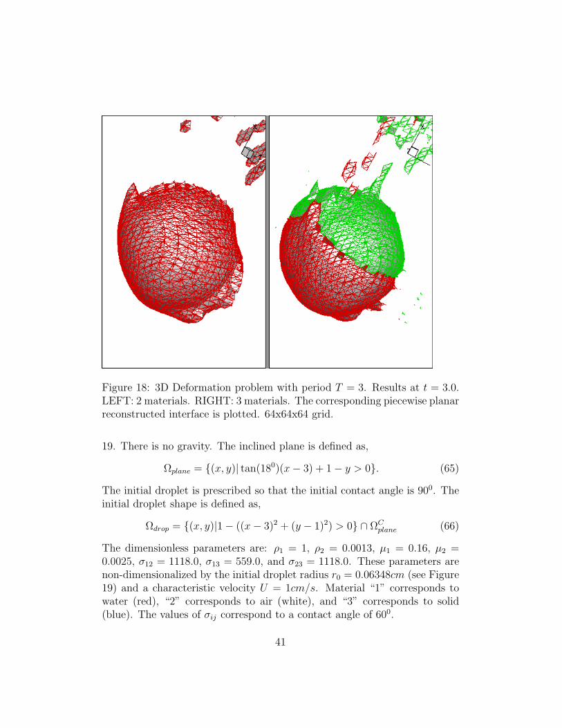
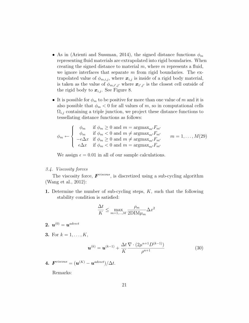
Figure 18: 3D Deformation problem with period T = 3. Results at t = 3.0.LEFT: 2 materials. RIGHT: 3 materials. The corresponding piecewise planarreconstructed interface is plotted. 64x64x64 grid.

19. There is no gravity. The inclined plane is defined as,

Ωplane = (x, y)| tan(180)(x− 3) + 1− y > 0. (65)

The initial droplet is prescribed so that the initial contact angle is 900. Theinitial droplet shape is defined as,

Ωdrop = (x, y)|1− ((x− 3)2 + (y − 1)2) > 0 ∩ ΩCplane (66)

The dimensionless parameters are: ρ1 = 1, ρ2 = 0.0013, µ1 = 0.16, µ2 =0.0025, σ12 = 1118.0, σ13 = 559.0, and σ23 = 1118.0. These parameters arenon-dimensionalized by the initial droplet radius r0 = 0.06348cm (see Figure19) and a characteristic velocity U = 1cm/s. Material “1” corresponds towater (red), “2” corresponds to air (white), and “3” corresponds to solid(blue). The values of σij correspond to a contact angle of 600.

41

The expected drop height is,

e0 = (1 + cos(π − θ))Rθ, (67)

and the expected base length is

L0 = 2 sin(π − θ)Rθ, (68)

where Rθ is the final radius,

Rθ =

√π

2θ − sin(2θ)R0. (69)

In table 3, we give the percent error for e0 and L0 when computed onsuccessively refined grids.

Table 3: Percent error for the relaxation of a water drop on a sloped inclinefrom a 900 contact angle to a 600 contact angle. The computational domain is6x3 in dimensionless units. The computational grid is a hierarchy of adaptive,dynamic, rectangular grids with a base coarse grid of 96x48 grid cells. Theerror is checked for 3 different grid resolutions.

Levels 100|e0−eexact0 |eexact0

100|L0−Lexact0 |Lexact0

1 3.4 4.02 0.9 1.43 0.4 0.3

4.4. Liquid Lens test problem

We repeat the Liquid Lens test problem as in (Kim, 2007) (section 4.4of (Kim, 2007)). Initially there are 3 materials with material 2 occupying acircle of diameter 0.3 in the center of the domain, material 1 occupying theremaining top half of the computational domain, and material 3 occupyingthe remaining bottom half of the computational domain. All 3 materialshave the same unit density and share the same viscosity of 1/60. The surfacetension coefficient between materials one and two and between materials twoand three was set to σ12 = 2/45 and σ23 = 2/45 respectively. We tested ouralgorithm for four different values of the surface tension between materialsone and three (σ13): σ13 = 3/90, 4/90, 5/90, and 6/90. The expected steady

42

Figure 19: Relaxation of droplet (red) on a slope (blue) from 900 contactangle to 600 contact angle. Base coarse grid is a rectangular 96x48 grid. Ef-fective fine grid resolution is 384x192. Left: initial conditions, Right: dropletat final static shape t = 0.8.

state solution has material 2 being stretched into a lens shape with majoraxis length of Lexact0 = 0.381, 0.416, 0.460, and 0.522 for the four cases ofσ13. In Figure 20 we illustrate the initial and steady state interfaces that wecompute using our multimaterial MOF method for the case when σ13 = 5/90.In Table 4, we give the percent error in major axis length for the four differentcases of σ13. In all of our test cases, the volume fluctuated by less than 0.001percent throughout the simulations.

4.5. Downward liquid jets

We study a downward liquid jet from a 3D round nozzle. Fig. 21 illus-trates the geometry of the nozzle and the computational conditions. Thegeometry of the nozzle can be defined by the nozzle diameter D and nozzleheight Hn. Uniform flow velocity is assigned at the nozzle inlet. Nonslipboundary condition is applied at the nozzle walls and top surface. Outflowboundary condition is applied on the rest boundaries.

The following fluid properties are used: water density ρl = 1.0×103 kg/m3

, air density ρg = 1.225 kg/m3 , water viscosity µl = 1.3× 10−3 kg/m.s , airviscosity µg = 2.0× 10−5 kg/m.s, surface tension σ = 7.28× 10−2 kg/s2 andthe gravitational acceleration g = 9.8 m/s2.

In the simulation the nozzle diameter D is 0.4 cm and the nozzle heightHn is 0.6 cm. Two levels of adaptive mesh refinement are used, resulting in

43

Figure 20: Stretching of a liquid lens. Red region indicates material 1, whiteregion is material 2 and blue region is material 3. All materials have thesame constant viscosity µ = 1/60. σ12 = 2/45, σ13 = 1/18, and σ23 = 2/45.The computational domain dimensions are 1x1. The base coarse grid is arectangular 64x64 grid. Effective fine grid resolution is 256x256. Left: initialconditions, Right: liquid lens at t = 6.

Inflow

D Hn

Outflow

Nonslip

Figure 21: Illustration of nozzle geometry and computational domain for adownward jet. D is the nozzle diameter and Hn is the nozzle height.

44

Table 4: Percent error for the stretching of a liquid lens at static shape.Initially material 2 is a circle centered at (1/2, 1/2), material 1 occupies theremaining top half, and material 3 occupies the remaining bottom half. Thedensity and viscosity is constant for all three materials: ρ = 1, µ = 1/60.The surface tension coefficients are σ12 = 2/45, σ23 = 2/45, and σ13 = 3/90,4/90, 5/90, and 6/90. The computational domain dimensions are 1x1. Thecomputational grid is a hierarchy of adaptive, dynamic, rectangular gridswith a base coarse grid of 64x64 grid cells and two levels of refinement.

σ13 L0 Lexact0 100|L0−Lexact0 |Lexact0

3/90 0.374 0.381 1.8%4/90 0.407 0.416 2.2%5/90 0.463 0.460 0.7%6/90 0.531 0.522 1.7%

a mesh which has 12 grid points per nozzle diameter.When the flow rate is lower, jet behavior is dominated by the gravita-

tional force and the surface tension force. Dripping regime will occur if thegravitational force is larger than the surface tension force. Fig. 22 shows thetime evolution of the dripping regime at a low nozzle inlet velocity of v0 = 6.0cm/s; When the flow rate is higher, the jet behavior is dominated by the iner-tial force and surface tension force, which leads to the jetting regime. Fig. 23shows the time evolution of the jetting regime at a high nozzle inlet velocityof v0 = 20.0 cm/s.

For purpose of generality, we introduce three non-dimensional parameters:the Reynolds number, the Weber number and the Ohnesorge number. TheReynolds number, Re = ρv0D/µ, gives a measure of the ratio of inertialforces to viscous forces. The Weber number, We = ρv2

0D/σ, represents therelative importance of inertia and surface tension. The Ohnesorge number,Oh =

√We/Re = µ/

√ρσD, relates viscous forces to the inertial and surface

tension forces.For the studied high inlet velocity case, the Reynolds number is 307,

the Weber number is 1.1 and the Ohnesorge number is 0.0034. The smallOhnesorge number means that the viscous forces are less important than theinertial force and surface tension. The breakup length, which is defined asthe distance between the nozzle tip and the point just before the first drop of

45

Figure 22: Snapshots of jet interface with a low velocity of v0 = 6.0 cm/s.

46

Figure 23: Snapshots of jet interface with a high velocity of v0 = 20.0 cm/s.

47

the liquid jet, can be computed using the following formula (Ashgriz, 2011):

L

D= 1.04C

√We (70)

where L is the jet breakup length, and C is an empirical parameter. (Grantand Middleman, 1966) suggested the value of C = 13 based on experimentaldata for Rayleigh breakup of low viscosity jets.

The computed breakup length, as shown in Fig. 23, is about 6 cm and itis very close to the value of 5.7 cm using Eq. 70.

4.6. Upward liquid jets

We simulate upward liquid jet based on a geometry shown in Fig. 24. InFig. 24 SLOW and SUP represent the lower and upper section of the nozzleoutlet respectively. Two different nozzle configurations are used in our sim-ulations. In the first case, both upper and lower surfaces are circles with thesame diameter of 3.2 mm. In the second case, the lower surface is a circle butthe upper surface is an ellipse which has the same cross sectional area as thelower surface and the ratio of its major axis and minor axis is 3. The nozzlehas an inlet of diameter (D) of 17.4 mm, a wall thickness H1 of 3 mm, anda height H2 of 9.4 mm. Three levels of adaptive mesh refinement are usedfor these cases and the effective grid size is about D1/10. i.e., 10 grid pointsper nozzle outlet diameter. The physical properties of the liquid and air arethe same as that in the downward jet example.

In the first case, a uniform velocity v0 = 4.0 cm is applied at the nozzleinlet. Fig. 25 shows the jet interface evolution with time. The maximum jetheight is 14 cm. The jet height first increase, reach the maximum height andthen decrease with water accumulating at the jet tip because of the gravityeffect.

In the second case the same nozzle inlet velocity of 4.0 cm/s is applied.Fig. 26 shows the jet interface evolution. It is noticed that after leaving thenozzle, the major axis and minor axis of the jet switch. This phenomenonwas discussed by (Lin, 2003) who argued that this switch is due to the effectof surface tension, which causes the jet section vibration about a equilibriumcircle shape.

4.7. Binary collisions of two water drops

Binary collisions of liquid drops have been experimentally studied by(Ashgriz and Poo, 1990) and (Orme, 1997) and numerically studied by (Tan-guy and Berlemont, 2005), (Chen and Yang, 2014), and (Nikolopoulos et al.,

48

D

H1

H2

SLOW

SUP

Figure 24: Illustration of nozzle geometry for upward jet. SUP is the uppersection of nozzle outlet, SLOW is the lower section of nozzle outlet, D is thediameter of nozzle inlet, H1 is the nozzle wall thickness and H2 is the nozzleheight.

Figure 25: Snapshots of upward liquid jet. A round nozzle is used.

49

Figure 26: Snapshots of upward liquid jet. The nozzle has a round lowsurface and an elliptical top surface

2009). For equal sized head-on collisions the outcomes depend on the Reynoldsnumber, Weber number which are defined as follows:

Re =ρdu

µWe =

ρdu2

σ

where ρ and µ are the liquid density and viscosity, respectively, d is thedrop diameter, u is the relative velocity of the two drops, and σ is the liquidsurface tension. With the Reynolds number in the range of 500 and 4000,Ashgriz and Poo found that the Reynolds number did not play a significantrole on the outcome (Ashgriz and Poo, 1990). In Figure 27, we show resultsof the simulation of the head-on collision of two equal sized water drops atthe Weber number of 25, 40 and 96. In the experiments, it was found thatreflexive separation occurs for a Weber number greater than nineteen andcoalescence or bouncing occurs for a Weber number less than twenty. Ournumerical results (Figure 27) corroborate these results.

4.8. Binary collisions of one water drop and one diesel drop

In Figure 28, we show results of the collision of a diesel oil drop with awater drop. These results can be compared with the experimental resultsreported by (Chen and Chen, 2006). As with the case for the collision of two

50

water drops, again we have agreement between simulation and experimentfor capturing the Weber number cutoff separating the coalescence regimefrom the reflexive separation regime.

4.9. Impingement of droplet on a thin liquid film

The complex phenomenon of droplet impingement on a thin film phe-nomenon is characterized by the Reynolds number Re, the Weber numberWe, the Ohnesorge number Oh and the nondimensional film thickness Hdefined as follows:

Re = ρv0D/µWe = ρv2

0D/σOh = µ/

√ρσD

H = h/D

(71)

where v0 is the impact velocity, D is the droplet diameter and h is the filmthickness. Also, a nondimensional time T = tv0/D is introduced and it is setto zero at the first contact between the droplet and the film.

At high We numbers, a crown structure is formed on the film surface andliquid jets or secondary droplets are splashed from the crown rim. This iscalled the splashing regime. At low We numbers, the droplet may depositon the film surface without secondary droplets. This is called the deposi-tion regime. The critical We number separating the splashing regime andthe deposition regime is studied by many researchers (Cossali et al., 1997;Okawa et al., 2006). Two Weber numbers are simulated: We = 100 whichcorresponds to the deposition regime and We = 600 which corresponds tothe splashing regime.

Fig. 29 shows the time evolution of the deposition process and Fig. 30shows the splashing process. The effective grid size is about D/70 for thedeposition case and D/135 for the splashing case. Different Rieber (Rieberand Frohn, 1999) who introduced random disturbance in his simulation, norandom disturbance was introduced in our simulation. The initial distancefrom the droplet to the film is 0.13D. For the deposition regime, as shownin Fig. 29, a crown-like structure is formed at the first stage of the impact.This crown-like structure travels outwards with a maximum crown height of0.5D without any secondary droplet splashing. For the splashing regime, asshown in Fig. 30, fingers are formed at the top of crown rim. These fingersare then breakup into secondary droplets due to Rayleigh instability.

51

Figure 27: Numerical simulation of head-on collision of two water drops.From top to bottom Weber Number is 15, 25, 40, and 96, respectively. Thecomputational grid is a block structured mesh with 16 cell per initial dropradius. One grid refinement is used(effective fine grid resolution is 32 cells perinitial drop radius). Results are in agreement with experiments (Ashgriz andPoo, 1990). We capture the correct transition point for reflexive separation.

52

Figure 28: Numerical simulation of head-on collision of a diesel oil drop(cyan) with a water drop (gold) and resulting encapsulation. Weber Num-ber equals 9.6, 45.3, and 58.9 for the top, middle and bottom rows respec-tively. Dimensionless drop diameter is 1 and computational domain size is0 < r < 1.3, −3.9 < z < 3.9. The computational grid is a block struc-tured dynamic adaptive mesh with 48x288 coarse grid cells and 2 additionallevels of adaptivity (effective fine grid resolution is 192x1152). Results arein agreement with experiments (Chen and Chen, 2006). We capture thecorrect transition point for reflexive separation. Simulations are done in 3daxisymmetric (RZ) coordinate system.

53

Figure 29: Snapshot of droplet-liquid film impingement, We = 100. Fromleft to right, top to bottom: T = 0.0, T = 1.0, T = 2.0, and T = 3.0

Figure 30: Snapshot of droplet-liquid film impingement, We = 600.

54

4.10. Impingement of droplet onto a solid wall

The impingement of a droplet on a smooth solid wall can result in differentregimes such as spreading, splashing, receding and rebounding (Yarin, 2006).The Weber number, Ohnesorge number as well as the contact angle play animportant role in the impact dynamics. We choose the droplet diameterD = 3.6 mm, density ρ = 1.0× 103 kg/m3, viscosity µ = 8.67× 10−4 kg/m.s,surface tension σ = 7.17 × 10−2 kg/s2 and impact velocity v0 = 0.77 m/s,which correspond to We = 30 and Oh = 0.0017. A dynamic contact anglemodel from (Jiang et al., 1979) is used, and the equilibrium contact angle isset to 87. Two levels of grid adaptation are used and the effective grid sizeis D/72.

Figure 31: Droplet impinging on a solid wall. Left, experimental results from(Kim and Chun, 2001). Right, present numerical results.

Figure 31 shows the evolution of the droplet shape. The computed dropletshape is also compared with experimental data from Kim and Chun(Kim andChun, 2001). As can be seen from Fig. 31, the experimental results and thenumerical results are in good agreement.

5. Concluding remarks

A new method was presented to study incompressible flows involvingmore than two materials. In this method, the MOF interface reconstructionmethod was used to capture the material interfaces. The directionally split

55

cell integrated semi-Lagrangian method was used to advect interfaces andmomentum. The block structured adaptive mesh refinement was used toincrease the resolution near material interfaces. Various 2D, 3D axisymmetricand 3D problems were simulated. Comparisons were made with analyticalor experimental results. Our simulation showed that the proposed methodis able to simulate multiphase problems involving more than two materials.The method is also able to capture the contact line dynamics and triplejunctions.

References

Ahn, H. T., Shashkov, M., 2007. Multi-material interface reconstruction ongeneralized polyhedral meshes. Journal of Computational Physics 226 (2),2096–2132.

Ahn, H. T., Shashkov, M., 2009. Adaptive moment-of-fluid method. Journalof Computational Physics 228 (8), 2792–2821.

Ahn, H. T., Shashkov, M., Christon, M. A., 2009. The moment-of-fluidmethod in action. Communications in Numerical Methods in Engineering25 (10), 1009–1018.

Almgren, A. S., Bell, J. B., Szymczak, W. G., 1996. A numerical methodfor the incompressible navier-stokes equations based on an approximateprojection. SIAM Journal on Scientific Computing 17 (2), 358–369.

Arienti, M., Sussman, M., 2014. An embedded level set method for sharp-interface multiphase simulations of diesel injectors. International Journalof Multiphase Flow 59, 1–14.

Ashgriz, N., 2011. Handbook of atomization and sprays. Springer.

Ashgriz, N., Poo, J., 1990. Coalescence and separation in binary collisions ofdroplets. J. Fluid Mech. 221, 183–204.

Aulisa, E., Manservisi, S., Scardovelli, R., Zaleski, S., 2007. Interface recon-struction with least-squares fit and split advection in three-dimensionalcartesian geometry. Journal of Computational Physics 225 (2), 2301 – 2319.URL http://www.sciencedirect.com/science/article/pii/S0021999107001325

56

Bell, J. B., Colella, P., Glaz, H. M., 1989. A second-order projection methodfor the incompressible navier-stokes equations. Journal of ComputationalPhysics 85 (2), 257–283.

Brackbill, J., Kothe, D. B., Zemach, C., 1992. A continuum method formodeling surface tension. Journal of computational physics 100 (2), 335–354.

Caboussat, A., Francois, M. M., Glowinski, R., Kothe, D. B., Sicilian, J. M.,2008. A numerical method for interface reconstruction of triple pointswithin a volume tracking algorithm. Mathematical and Computer Mod-elling 48 (11), 1957–1971.

Chen, R.-H., Chen, C.-T., 2006. Collision between immiscible drops withlarge surface tension difference: diesel oil and water. Experiments in Fluids41, 453–461.

Chen, X., Yang, V., 2014. Thickness-based adaptive mesh refinementmethods for multi-phase flow simulations with thin regions. Journal ofComputational Physics 269 (0), 22 – 39.URL http://www.sciencedirect.com/science/article/pii/S0021999114001612

Chenadec, V. L., Pitsch, H., 2013. A 3d unsplit forward/backward volume-of-fluid approach and coupling to the level set method. Journal of Compu-tational Physics 233 (0), 10 – 33.

Chorin, A. J., October 1968. Numerical solution of the Navier-Stokes equa-tions. Journal of Computational Physics 22, 745–762.

Cossali, G., Coghe, A., Marengo, M., 1997. The impact of a single drop on awetted solid surface. Experiments in fluids 22 (6), 463–472.

Desjardins, O., Moureau, V., Pitsch, H., 2008. An accurate conservativelevel set/ghost fluid method for simulating turbulent atomization. Journalof Computational Physics 227 (18), 8395–8416.

Duffy, A., Kuhnle, A., Sussman, M., 2012. An improved variabledensity pressure projection solver for adaptive meshes, unpublished.http://www.math.fsu.edu/sussman/MGAMR.pdf.

57

Dyadechko, V., Shashkov, M., 2005. Moment-of-fluid interface reconstruc-tion. Los Alamos report LA-UR-05-7571.

Dyadechko, V., Shashkov, M., 2008. Reconstruction of multi-material in-terfaces from moment data. Journal of Computational Physics 227 (11),5361–5384.

Grant, R. P., Middleman, S., 1966. Newtonian jet stability. AIChE Journal12 (4), 669–678.

Hirt, C. W., Nichols, B. D., 1981. Volume of fluid (vof) method for thedynamics of free boundaries. Journal of computational physics 39 (1), 201–225.

Jemison, M., Loch, E., Sussman, M., Shashkov, M., Arienti, M., Ohta, M.,Wang, Y., 2013. A coupled level set-moment of fluid method for incom-pressible two-phase flows. Journal of Scientific Computing 54 (2-3), 454–491.

Jemison, M., Sussman, M., Arienti, M., 2014. Compressible, multiphase semi-implicit method with moment of fluid interface representation. Journal ofComputational Physics 279, 182–217.

Jemison, M., Sussman, M., Shashkov, M., 2015. Filament capturing with themultimaterial moment-of-fluid method. Journal of Computational Physics.

Jiang, T.-S., Soo-Gun, O., Slattery, J. C., 1979. Correlation for dynamiccontact angle. Journal of Colloid and Interface Science 69 (1), 74–77.

Kang, M., Fedkiw, R. P., Liu, X.-D., 2000. A boundary condition capturingmethod for multiphase incompressible flow. Journal of Scientific Comput-ing 15 (3), 323–360.

Kim, H.-Y., Chun, J.-H., 2001. The recoiling of liquid droplets upon collisionwith solid surfaces. Physics of fluids 13, 643.

Kim, J., 2007. Phase field computations for ternary fluid flows. Computermethods in applied mechanics and engineering 196, 4779–4788.

Kucharik, M., Garimella, R. V., Schofield, S. P., Shashkov, M. J., 2010. Acomparative study of interface reconstruction methods for multi-materialale simulations. Journal of Computational Physics 229 (7), 2432–2452.

58

Kwatra, N., Su, J., Gretarsson, J. T., Fedkiw, R., 2009. A method for avoid-ing the acoustic time step restriction in compressible flow. Journal of Com-putational Physics 228 (11), 4146–4161.

Li, X., Arienti, M., Soteriou, M. C., Sussman, M., 2010. Towards an effi-cient, high-fidelity methodology for liquid jet atomization computations.In: AIAA Aerospace Sciences Meeting.

Lin, S.-P., 2003. Breakup of liquid sheets and jets. Cambridge UniversityPress New York.

Liovic, P., Rudman, M., Liow, J.-L., Lakehal, D., Kothe, D., 2006. A 3dunsplit-advection volume tracking algorithm with planarity-preserving in-terface reconstruction. Computers & fluids 35 (10), 1011–1032.

Menard, T., Tanguy, S., Berlemont, A., 2007. Coupling level set/vof/ghostfluid methods: Validation and application to 3d simulation of the primarybreak-up of a liquid jet. International Journal of Multiphase Flow 33 (5),510–524.

Nikolopoulos, N., Nikas, K.-S., Bergeles, G., 2009. A numerical investigationof central binary collision of droplets. Computers and Fluids 38 (6), 1191– 1202.URL http://www.sciencedirect.com/science/article/pii/S0045793008002296

Noel, E., Berlemont, A., Cousin, J., Menard, T., 2012. Application of the im-mersed boundary method to simulate flows inside and outside the nozzles.ICLASS 2012, 12th Triennial International Conference on Liquid Atom-ization and Spray Systems, Heidelberg, Germany, September 26.

Okawa, T., Shiraishi, T., Mori, T., 2006. Production of secondary drops dur-ing the single water drop impact onto a plane water surface. Experimentsin fluids 41 (6), 965–974.

Orme, M., 1997. Experiments on droplet collisions, bounce, coalescence anddisruption. Prog. Energy Combust. Sci. 23, 65–79.

Osher, S., Fedkiw, R. P., 2001. Level set methods: an overview and somerecent results. Journal of Computational physics 169 (2), 463–502.

59

Osher, S., Sethian, J. A., 1988. Fronts propagating with curvature-dependentspeed: algorithms based on hamilton-jacobi formulations. Journal of com-putational physics 79 (1), 12–49.

Palacios, J., Gomez, P., Zanzi, C., Lopez, J., Hernandez, J., 2010. Exper-imental study on the splash/deposition limit in drop impact onto solidsurfaces. Proceedings of 23rd ILASS-2010, Brno, Czech Republic.

Pilliod Jr, J. E., Puckett, E. G., 2004. Second-order accurate volume-of-fluid algorithms for tracking material interfaces. Journal of ComputationalPhysics 199 (2), 465–502.

Raessi, M., 2008. A level set based method for calculating flux densities intwo-phase flows. Annual Research Briefs (Center for Turbulence Research,Stanford).

Raessi, M., Pitsch, H., 2009. Modeling interfacial flows characterized by largedensity ratios with the level set method. Annual Research Brief, Centerfor Turbulence Research.

Rayleigh, L., 1878. On the instability of jets. Proceedings of the LondonMathematical Society, 4–13.

Rieber, M., Frohn, A., 1999. A numerical study on the mechanism of splash-ing. International Journal of Heat and Fluid Flow 20 (5), 455–461.

Rudman, M., 1998. A volume-tracking method for incompressible multifluidflows with large density variations. International Journal for NumericalMethods in Fluids 28 (2), 357–378.

Sallam, K., Aalburg, C., Faeth, G., 2004. Breakup of round nonturbulentliquid jets in gaseous crossflow. AIAA journal 42 (12), 2529–2540.

Sallam, K., Dai, Z., Faeth, G., 1999. Drop formation at the surface of planeturbulent liquid jets in still gases. International journal of multiphase flow25 (6), 1161–1180.

Scardovelli, R., Zaleski, S., 2003. Interface reconstruction with least-squarefit and split eulerian–lagrangian advection. International Journal for Nu-merical Methods in Fluids 41 (3), 251–274.

60

Schofield, S. P., Garimella, R. V., Francois, M. M., Loubere, R., 2008. Ma-terial order-independent interface reconstruction using power diagrams.International Journal for Numerical Methods in Fluids 56 (6), 643–659.URL http://dx.doi.org/10.1002/fld.1544

Schofield, S. P., Garimella, R. V., Francois, M. M., Loubere, R., 2009. Asecond-order accurate material-order-independent interface reconstructiontechnique for multi-material flow simulations. Journal of ComputationalPhysics 228 (3), 731 – 745.URL http://www.sciencedirect.com/science/article/pii/S0021999108005081

Sijoy, C., Chaturvedi, S., 2010. Volume-of-fluid algorithm with differentmodified dynamic material ordering methods and their comparisons.Journal of Computational Physics 229 (10), 3848 – 3863.URL http://www.sciencedirect.com/science/article/pii/S0021999110000549

Son, G., Hur, N., 2002. A coupled level set and volume-of-fluid method forthe buoyancy-driven motion of fluid particles. Numerical Heat Transfer:Part B: Fundamentals 42 (6), 523–542.

Stewart, P., Lay, N., Sussman, M., Ohta, M., 2008. An improved sharpinterface method for viscoelastic and viscous two-phase flows. Journal ofScientific Computing 35 (1), 43–61.

Sussman, M., 2003. A second order coupled level set and volume-of-fluidmethod for computing growth and collapse of vapor bubbles. Journal ofComputational Physics 187 (1), 110–136.

Sussman, M., 2005. A parallelized, adaptive algorithm for multiphase flowsin general geometries. Computers and Structures 83, 435–444.

Sussman, M., Almgren, A. S., Bell, J. B., Colella, P., Howell, L. H., Welcome,M. L., 1999. An adaptive level set approach for incompressible two-phaseflows. Journal of Computational Physics 148 (1), 81–124.

Sussman, M., Fatemi, E., Smereka, P., Osher, S., 1998. An improved levelset method for incompressible two-phase flows. Computers & Fluids 27 (5),663–680.

61

Sussman, M., Ohta, M., 2009. A stable and efficient method for treatingsurface tension in incompressible two-phase flow. SIAM J. Sci. Comput.31 (4), 2447–2471.

Sussman, M., Puckett, E. G., 2000. A coupled level set and volume-of-fluid method for computing 3d and axisymmetric incompressible two-phaseflows. Journal of Computational Physics 162 (2), 301–337.

Sussman, M., Smereka, P., Osher, S., 1994. A level set approach for comput-ing solutions to incompressible two-phase flow. Department of Mathemat-ics, University of California, Los Angeles.

Tanguy, S., Berlemont, A., 2005. Application of a level set method forsimulation of droplet collisions. International Journal of Multiphase Flow31 (9), 1015 – 1035.URL http://www.sciencedirect.com/science/article/pii/S0301932205000832

Taylor, G., 1963. Generation of ripples by wind blowing over viscous fluid.The Scientific Papers of GI Taylor, 244–254.

Wang, Y., Simakhina, S., Sussman, M., 2012. A hybrid level set-volumeconstraint method for incompressible two-phase flow. Journal of Compu-tational Physics.

Wang, Z., Yang, J., Koo, B., Stern, F., 2009. A coupled level set and volume-of-fluid method for sharp interface simulation of plunging breaking waves.International Journal of Multiphase Flow 35 (3), 227–246.

Weymouth, G., Yue, D. K.-P., 2010. Conservative volume-of-fluid methodfor free-surface simulations on cartesian-grids. Journal of ComputationalPhysics 229 (8), 2853–2865.

Yarin, A., 2006. Drop impact dynamics: splashing, spreading, receding,bouncing. Annu. Rev. Fluid Mech. 38, 159–192.

62