multiphase enkf

International Journal of Multiphase Flow 29 (2003) 1283–1309www.elsevier.com/locate/ijmulflow

Tuning of parameters in a two-phase flow model usingan ensemble Kalman filter

R.J. Lorentzen a,*, G. Nævdal a, A.C.V.M. Lage b

a RF-Rogaland Research, Thormøhlensgt. 55, N-5008 Bergen, Norwayb Petrobras, Research and Development center (CENPES), Cidade Universit�aaria, Q.7 Ilha do Fund~aao 21949-900,

Rio de Janeiro, Brazil

Received 1 September 2002; received in revised form 24 April 2003

Abstract

A new methodology for online tuning of model parameters in a two-phase flow model by taking intoaccount measured data is presented. Important model parameters are tuned using the ensemble Kalman

filter. The present study is motivated by applications in underbalanced drilling, although the idea of using

the ensemble Kalman filter in tuning of model parameters should be of interest in a wide area of appli-

cations. A description of modeling of the two-phase flow in the well is presented, as well as the imple-

mentation of the ensemble Kalman filter. The performance of the filter is studied, both using synthetic and

experimental data.

� 2003 Elsevier Ltd. All rights reserved.

Keywords: Ensemble Kalman filter; Two-phase flow; Well-flow modeling

1. Introduction

The development of increased computer power and advances in measuring techniques give newopportunities in online tuning of complex models. Within atmospheric and oceanic literaturethere has been a strong interest in data assimilation during the last decade. This has resulted in theadaption of Kalman filter techniques to large-scale non-linear models. The use of these Kalmanfilter techniques within other areas seems to be a promising area of research. In this paper we will

*Corresponding author. Fax: +47-55543860.

E-mail address: [email protected] (R.J. Lorentzen).

0301-9322/03/$ - see front matter � 2003 Elsevier Ltd. All rights reserved.

doi:10.1016/S0301-9322(03)00088-0

mail to: [email protected]

1284 R.J. Lorentzen et al. / International Journal of Multiphase Flow 29 (2003) 1283–1309

demonstrate how the ensemble Kalman filter can be used to tune model parameters of a two-phase flow system.

Modeling of two-phase flow is a difficult task, and simplifications have to be done. In thepresent application we study two-phase flow in wells. As a simplification we treat this as an onedimensional problem using a model obtained from cross sectional averaging of the Navier–Stokesequations, replacing second order diffusion terms by empirical correlations (including modelparameters) which are flow regime dependent. These correlations are obtained from laboratoryexperiments conducted in different surroundings than real full-scale facilities, and possibilities ofinaccuracies due to system dependencies does therefore exist. It is crucial to use all availableinformation to tune the model parameters, as their values have large impact on the behaviour ofthe system. In particular it is useful to do online tuning, to exploit the current measurements. Weshow that such tuning can be done using a Kalman filter approach by including model parametersin the state vector of the system. The parameters are then updated as new measurements becomeavailable. In this paper we will show that the model parameters we chose are updated satisfac-torily, leading to improved forecasts of the future flow.

Several Kalman filter techniques have been developed to work with large-scale non-linearsystem. We have implemented the ensemble Kalman filter, first introduced by Evensen (1994).The ensemble Kalman filter is based on a Monte-Carlo approach, using an ensemble of modelrepresentations to build up the necessary statistics. The ensemble Kalman filter is easy to im-plement and handles strong non-linearities better than other known Kalman filter techniques forlarge-scale problems (Verlaan and Heemink, 2001). There is a lot of ongoing work within me-teorology and oceanography using Kalman filter techniques, both using ensemble Kalman filterand other techniques. Some recent works in this direction are (e.g. Verlaan and Heemink, 2001;Anderson, 2001; Hamil et al., 2001). We refer to these works, and the works cited therein forthose who are interested in the state of the art of the research on Kalman filter for large-scalenon-linear models.

To our knowledge, there has been a limited number of applications on ensemble Kalman filtertechniques for tuning model parameters. In the above mentioned works, the focus is on im-proving the estimate of the state variables, although the tuning of one model parameter is dis-cussed using an ensemble adjustment Kalman filter in Anderson (2001). (The ensembleadjustment Kalman filter is a slight modification of the ensemble Kalman filter.) Here we will usethe ensemble Kalman filter to tune nine model parameters. The promising result of the presentwork has motivated further studies in using the ensemble Kalman filter for tuning of modelparameters. In Nævdal et al. (2002a,b) the tuning of the permeability field in a porous mediamodel is studied.

The setup of our model is motivated by applications within underbalanced drilling. The en-semble Kalman filter was used for tuning of the model parameters in Lorentzen et al. (2001a). Inthat study, using both synthetic and full-scale experimental data, we showed that the tuningimproved the fitting of the data, and that more reliable predictions were obtained. Here we bothpresent results from a study on the robustness of the methodology, using synthetic data, as well assome more results with full-scale experimental data. An alternative to using the ensemble Kalmanfilter to tune the model parameters is to use a least square approach. This technique was exploitedin Lorentzen et al. (2001b). The least square approach is, however, more computationally de-manding, and seems therefore not to be suitable to online tuning (Lorentzen, 2002).

R.J. Lorentzen et al. / International Journal of Multiphase Flow 29 (2003) 1283–1309 1285

We will study the robustness of the ensemble Kalman filter using synthetic data. Measurementsare generated synthetically using different sets of model parameters. It is shown that by using theensemble Kalman filter the model parameters are tuned so that the measurements are fitted, andreasonable predictions are obtained, thereby giving evidence for the robustness of the ensembleKalman filter. Although the final judgment of the methodology has to be based on its perfor-mance on real data, the use of synthetic data give some more possibilities in judging the results.After studying the robustness of the approach using synthetic data, we present results using a setof experimental data.

The paper is organized as follows. In Section 2 the physical model is presented. In Section 3 theimplementation of the ensemble Kalman filter is presented. For the convenience of the reader, aself-contained presentation of the ensemble Kalman filter in general is included. In Section 4 wediscuss the details of the chosen variables (including different covariance matrices) in the setup ofthe filter for the present application and present the results.

2. Dynamic model

A model describing one-dimensional two-phase flow in pipelines consists of non-linear partialdifferential equations describing mass, momentum and energy balances for each of the phases (seee.g. Ishii, 1975). This model is obtained from cross sectional averaging of the Navier–Stokesequations and replacing second order diffusion terms by empirical correlations which are flowregime dependent. The dynamics of multiphase flow are determined by these balance equationswhich involve complicated terms for interface exchanges of mass, momentum and energy. Inaddition, wall friction and volumetric forces like gravity are highly responsible for the develop-ment of the flow.

The focus of this work is the application of filter techniques rather than a detailed fluid de-scription, and we limit ourselves to consider gas–liquid flow in vertical wells. We assume that nomass enters or leaves the system through the pipe walls, and we neglect mass transfer between thephases. The simplified mass conservation equations are then written

o

otðakAqkÞ þ

o

osðakAqkvkÞ ¼ 0; k ¼ l; g; ð1Þ

where l, g represents the liquid and gas phase respectively, t denote the time variable, a is thevolume fraction, A is cross-section area, q is the density, s denote the coordinate along the pipeand v is the velocity.

The fundamental two-phase model consists of separate momentum conservation equations foreach phase, and includes complicated terms related to phase interaction. It is however a commonpractice in two-phase modeling to add the momentum equations together, which causes thedifficult phase interaction terms to cancel (see Fjelde, 2000; Faille and Heintz�ee, 1999; Pauchonet al., 1994). This results in the following simplified equation for the mixture phase (drift fluxformulation):

o

otAðalqlvl þ agqgvgÞ þ

o

osAðalqlv

2l þ agqgv

2gÞ þ A

o

osp ¼ �AðK � qmixg sin hÞ; ð2Þ


where p is the pressure, K is a friction pressure loss term, h is the well inclinationand qmix ¼ qgag þ qlal is the mixture density. We further assume that there is no heat ex-change in the fluid, which makes the energy conservation equation redundant (isentropicflow).

The stated governing partial differential equations for the two-phase flow are insufficient tocompletely describe the physical processes involved. There are more unknowns than equationsand thus closure conditions are required. The missing information in the mixture momentumequation must be replaced by empirical closure relations which provide information about phasevelocities and pressure loss terms. These relations consist of complicated time-dependent equa-tions (see e.g. Franca and Lahey, 1992; Bendiksen, 1984; Cassaude et al., 1989; Lage, 2000) andinclude several parameters which are only approximately known. Inaccuracies in these parametersrelates to system dependencies such as complex fluid properties, geometry, impurities in the fluids,flow regime (laminar/turbulent) and unknown pipe properties. The object of this paper is to showhow measurements can be used to improve these parameters, leading to better forecasts of thetwo-phase flow. We consider one set of simple closure relations for downward two-phase flow inthe drillstring, and a more sophisticated mechanistic model for upward two-phase flow in theannulus. This model takes into account the complex and regime-dependent relations for the phasevelocities and pressure loss terms.

In addition to closure relations describing phase velocities it is necessary to specify thermo-dynamic relations, generally derived by assuming a system in thermodynamic equilibrium (PVT-models). In this work, the PVT-models are obtained by assuming an ideal gas law and a liquiddensity model with fixed compressibility. It is also necessary to provide boundary conditions forthe system. In this context, the flow rates are assumed to be known at the inlet, and the pressure isassumed to be given at the outlet.

2.1. Closure relations for downward two-phase flow in the drillstring

In the standard drift-flux approach, the closure of the system is achieved by specifying a slipmodel between the phases:

vg ¼ C0;dðagvg þ alvlÞ þ C1;d ¼ C0;dvmix þ C1;d : ð3Þ

In addition, it is necessary to provide an appropriate model for the frictional pressure loss term inthe momentum equation. A frequently used expression for this term is

K ¼ C2;d2fD

qmixv2mix; ð4Þ

where f is a known flow dependent friction factor, D is the pipe diameter and vmix ¼ vgag þ vlal isthe mixture velocity. In Eqs. (3) and (4), the factors C0;d , C1;d and C2;d are assumed to be givenparameters, and are among the parameters which are tuned by the filter technique described insubsequent sections.


2.2. Mechanistic model for upward two-phase flow in the annulus

Mechanistic models have become quite popular for describing steady-state two-phase flow inproducing wells. The mechanistic models provide information about flow patterns, pressure dropsand phase velocities:

MðD1;D2; ql;qg; s;ll; lg; qmix; ag; alÞ ! ðvg; vl; pressure lossÞ; ð5Þ

where D1 and D2 are the inner and outer diameter respectively, ll and lg are the viscosities for theliquid and gas phase, s is the interfacial tension and qmix ¼ qgagvg þ qlalvl is the mixture mo-mentum. Furthermore, it is possible to integrate these mechanistic steady-state procedures intofully dynamic two-phase flow models to provide the necessary information regarding phase ve-locities and pressure loss terms (see e.g. Pauchon et al., 1994; Lage et al., 2000a,b; Bendiksen et al.,1991). We have implemented a recently developed mechanistic model for two-phase flow in an-nulus, described in the work by Lage (2000), Lage and Time (2000).

A mechanistic model consists of basically two parts, where one part is composed of criteria forpredicting the flow pattern. The other part consists of models for treating each specific pattern.The framework developed by Taitel and Barnea (1983) is the basis for the definition of thetransition criteria. They considered five different flow configurations (bubble, dispersed bubble,slug, churn and annular) for upward two-phase flow in pipes and formulated boundaries betweenthem. Although the implemented method include all five configurations, we limit the followingpresentation to bubble flow and slug flow. These flow regimes are dominant in the examples wehave considered, and parameters related to these regimes are tuned by the ensemble Kalman filterpresented in Section 3.

2.2.1. Bubble flow model

Harmathy (1960) proposed

v01 ¼ C1;b1:53ðql � qgÞgs

q2l

� �0:25ð6Þ

for the rise velocity of a single bubble rising in an infinite medium, with C1;b ¼ 1. It is only afunction of the physical properties of gas and liquid. However, Wallis (1969) proposed that for abubble rising in a swarm of bubbles, Eq. (6) should be corrected by

v0 ¼ v01ð1� agÞn; ð7Þ

where the exponent n is assumed to be known.The slippage between gas and liquid phases is the key aspect to be considered for determining

the flow parameters. As suggested by Papadimitriou and Shoham (1991), the slip velocity is de-fined as

vg ¼ v0 þ C0;bvmix:


This equation is used to calculate the unknownphase velocities. The friction pressure loss is given by

K ¼ C2;b2fDh

qmixv2mix;

where Dh is the difference between the outer and inner diameter. The parameters C0;b, C1;b and C2;b

are added to the vector of parameters which is tuned by the ensemble Kalman filter.

2.2.2. Slug flow modelFig. 1 presents a schematic diagram of an idealized slug unit in an annulus. Large Taylor

bubbles of length ltb, move upward, and Kelessidis and Dukler (1989) proposed the followingexpression for the translational velocity vtb:

vtb ¼ C0;svmix þ C1;s0:35ffiffiffiffiffiffiffiffiffiffiffiffiffiffiffiffiffiffiffiffiffiffiffigðD1 þ D2Þ

p;

with C0;s ¼ 1:2 and C1;s ¼ 1. The Taylor bubbles are followed by liquid slugs containing small,uniformly distributed bubbles with an average gas fraction ag;ls ¼ 0:2. By integrating over theentire slug unit, the following equation for the gas velocity is obtained:

vg ¼ vtb �ag;lsag

ðvtb � vg;lsÞ;

where ls indicates the value of the flow variable in the liquid slug zone. The gas velocity in theliquid slug zone (vg;ls) is found by using vmix and the equations derived for bubble flow. The liquidvelocity is then found by substituting vg in the expression for qmix. A detailed discussion ofmodeling of slug flow, and choice of parameters values, is found in Bendiksen et al. (1996).

A mass balance calculation for the slug unit provides values for the length of the slug unit andthe length of the liquid slug. All the parameters are then available for the pressure drop calcu-lations. The friction pressure gradient is evaluated in the liquid slug zone as

K ¼ C2;s2fDh

qmixv2mix

llslsu

:

Fig. 1. Slug flow structure.


The parameters C0;s, C1;s and C2;s complete the list of parameters which are tuned by the ensembleKalman filter.

2.2.3. Transition regime

In order to ensure a smooth development of the two-phase flow, the mechanistic model uses atransition regime between the bubble flow regime and the slug flow regime. The transition regimeis modeled by performing interpolations of the flow variables resulting from the bubble flowmodel and the slug flow model.

2.3. Numerical scheme

The non-linear and coupled characteristic of the drift-flux model makes it impossible to solvethe equations analytically, and a numerical solution strategy is required. The aim of the numericalsolver is to compute accurate and stable approximations of the flow variables (e.g. pressure,velocity, volume fractions etc.). Numerical methods replace the continuous problem representedby the Eqs. (1) and (2) by a finite set of discrete values.

The drift-flux model can be written as a system of conservation laws which has been analyzedby Th�eeron (1989) and Gavage (1991). The model was shown to be hyperbolic in a physicallyreasonable region of parameters and three distinct and real eigenvalues were obtained under themain assumption that the liquid phase was considered incompressible. Two of the eigenvalues (k1and k3) correspond to rapid pressure waves propagating in the upstream and downstream di-rection of the fluid flow, while the last eigenvalue (k2) is associated to gas volume waves and equalto the gas velocity. The eigenvalues corresponding to the pressure pulses are generally 10–100times bigger than the eigenvalue corresponding to the mass transport, i.e. jk1j; jk3j � jk2j.

We have chosen a numerical method which follows the idea described in Frøyen et al. (2000). Itis a semi-implicit solution strategy which treats the acoustic signals associated with k1 and k3implicit while maintaining the explicit treatment of the mass transport. The time step is thuslimited by the time interval the mass transport signal use to traverse a grid block. Some of thesolution details are thus sacrificed to increase computational efficiency. This method has beentested against experimental data in an underbalanced drilling scenario in Lage et al. (2000b).

3. Estimation theory

In the models presented in Section 2 there are some influential parameters which are uncertain.Improved knowledge on the value of these parameters leads to significantly better predictions ofthe system behavior. There are several approaches available to fit these parameters. In Lorentzenet al. (2001a) the parameters were fitted using the ensemble Kalman filter. A minimization be-tween the model output and measurements using a least squares approach was pursued in Lo-rentzen et al. (2001b). Here, we will continue the studies from Lorentzen et al. (2001a), and studythe robustness of the ensemble Kalman filter in the tuning of the model parameters, in addition topresenting more results using experimental data.

The Kalman filter was initially developed for the discrete-data linear filtering problem. Anintroduction to the general idea of the Kalman filter can be found in Maybeck (1979). As the


measurements become available, they are used to estimate the state of the process. (The states ofthe system are the time dependent variables.) It is straightforward to extend the state variableswith model parameters, by treating the model parameters as time dependent variables. TheKalman filter has been the subject of extensive research, and several adaptions to non-linearsystems have been developed. A recent approach which has been applied successfully for large-scale non-linear models within oceanographic modeling is the ensemble Kalman filter, first in-troduced in Evensen (1994).

For the convenience of the reader we present our implementation of the ensemble Kalmanfilter. The filter can be divided in two steps, a forecast step and an analysis step. In the forecaststep the state of the system is updated by solving the dynamic model as described in Section 2. Inthe analysis step the state of the model is updated to take into account the measurements. Thestate vector after running the forecast step is denoted byWf

k, the state vector after the analysis stepby Wa

k .The ensemble Kalman filter is based on a Monte-Carlo approach, using an ensemble of

model representations to evaluate the necessary statistics. We have used 100 members in theensemble. We selected this size of the ensemble since an ensemble size of this order have beenfound to be sufficient for much larger atmospheric models (Houtekamer and Mitchell, 1998).The influence of the size of the ensemble on the performance of the ensemble Kalman filter forthis application is a topic worthwhile further research. The experience in using the ensembleKalman filter for parameter estimation and also for tuning of multiphase flow models islimited.

The forecast step consists in running the model (i.e. the simulator developed as described inSection 2.3), which we denote by f, one time step for each member of the ensemble. For the i�thmember of the ensemble at time step k, we denote the forecast state vector by Wf

k;i and the ana-lyzed state by Wa

k;i. In the forecast step the simulator is run from the current time (say timestepk � 1) to the point in time where the next measurement becomes available (timestep k). Thesimulator is run once for each member of the ensemble using the analyzed state Wa

k�1;i as initialvalue. In addition to the updating of the state given by the simulator, random model noise isadded. This gives the equation

Wfk;i ¼ fðWa

k�1;iÞ þ emk;i; ð8Þ

where emk;i � Nð0;QkÞ. The notation emk;i � Nð0;QkÞ denotes that the model noise is generated bydrawing realizations from a Gaussian distribution with zero mean and covariance matrix Qk.Here the distribution of the model noise may be time dependent. The time dependence of thedistribution of the model noise is due to the fact that the covariance matrix Q may be time de-pendent.

The filter is initialized by generating an initial ensemble. This is done by specifying a meanvalue, Wa

0 and a covariance matrix, Q0 of the initial ensemble. The mean value of the initial en-semble should preferably be a good estimate of the initial true state. The members of the en-sembles are then drawn randomly assuming a Gaussian distribution,

Wa0;i ¼ Wa

0 þ em0;i; ð9Þ

where em0;i � Nð0;Q0Þ.


The analyzed state at time step k is computed by taking into account the measurement vector attime step k. We assume that there is a linear relationship between the measurements, dk, and thestates, Wk, expressed by the equation

dk ¼ HWk: ð10Þ
The above equation refers to an idealized situation with no noise and no representation error inthe measurements. We assume that these effects can be expressed by a Gaussian random variablewith zero mean and covariance matrix Rk. The index k is included since the covariance matrix ofthe measurement noise may be time dependent, for instance when the measurement accuracy isgiven as a relative accuracy. We assume that there is no correlation in the noise of measurementstaken at different time steps.
As pointed out in Burgers et al. (1998) it is necessary to define new observations for propererror propagation in the ensemble Kalman filter. The actual measurement dk serves as the ref-erence observation. For each member of the ensemble an observation vector dk;i is generatedrandomly as

dk;i ¼ dk þ eok;i;

where eok;i � Nð0;RkÞ.To apply the Kalman filter, the error covariance matrix for the model is needed. In the Kalman

filter this is defined in terms of the true state as the expectation

EððWfk �Wt

kÞðWfk �Wt

kÞÞ:

Since the true state is not known, we approximate the true state by the mean of the ensemble

Wtk �

cWfkWfk ¼

1

N

XNi¼1

Wfk;i;

where N is the sample size of the ensemble. With this approximation of the true state, an ap-proximation of a left factor of the error covariance matrix of the model is

Lfk ¼

1ffiffiffiffiN

p Wfk;1 �

cWfkWfk

� �Wf

k;2 �cWf

kWfk

� �. . . Wf

k;N � cWfkWfk

� �h i:

The approximation of the model error covariance matrix then becomes

Pfk ¼ Lf

kðLfkÞ

T: ð11Þ

The expression of the Kalman gain matrix is (see e.g. Maybeck, 1979)

Kk ¼ PfkH

TðHPfkH

T þ RkÞ�1:

The analyzed state of each member of the ensemble is computed as

Wak;i ¼ Wf

k;i þ Kkðdk;i �HWfk;iÞ:

The analyzed error covariance matrix, Pak , of the model can be computed along the same lines as

Pfk. Since the updating of the ensemble is linear, the new estimate of the true state, based on the

ensemble after the analysis step is


Wtk � cWa

kWak ¼

cWfkWfk þ Kk dk

��HcWf

kWfk

�;

and the model error covariance matrix after the analysis step is

Pak ¼ ðI� KkHÞPf

k:

The underlying assumptions behind the filter are that there is zero covariance between the modelerror and the measurement error and that both the model error and measurement error are un-correlated in time. For the practical implementation of the above procedure, it is important tobear in mind that while evaluating the Kalman gain matrix, Pf

k should be entered factorized as in(11), and the product should be evaluated in an order such that the dimensions of temporarymatrices are kept as low as possible.

4. Results

In this section we present and discuss examples which demonstrate the filter technique de-scribed above. Details regarding discretization, model error and measurement error are outlinedin Sections 4.1–4.3. Section 4.4 contains two examples where two sets of model parameters areused to generate synthetic measurements. The ability to reconstruct the parameters by using theensemble Kalman filter is then investigated, and forecasts using the estimated parameters arecompared to the synthetic measurements. Section 4.5 contains an example where full-scale ex-perimental measurements are used to tune the model parameters. A forecast of the two-phase flowis then compared to the measurements.

4.1. Discretization and state vector

Use of a numerical method requires a discretization of the time and space variables. We haveused a spatial discretization where Ds ¼ 20 m. Furthermore, a maximum value of 15 m/s is as-sumed for the gas velocity, which gives a maximum valid time-step Dt ¼ Ds=15 s � 1:3 s.

By using the ensemble Kalman filter it is possible to combine the information obtained from themeasurements with the model to get an improved estimation of the state vector. The state vector(W) is composed of discretized pressure values and discretized gas and liquid mass rates. This ismotivated by the fact that these variables are usually measured at some positions during drillingoperations. The observation operator (H) is then composed by choosing the matrix which selectsthe values from the state vector corresponding to the measurements. In addition, the state vectorincludes several parameters from the closure relations related to drillstring and annulus. The statevector is then defined as

W ¼ v p½ �T;

where

v ¼ � � � pJ FJR;g FJR;l � � �½ �


and

p ¼ C0;d C1;d C2;d C0;b C1;b C2;b C0;s C1;s C2;s½ �:
Here J indicates the cell number, pJ is the average pressure value of the cell, and FJR;g and FJR;l arethe mass rate of gas and liquid, evaluated at the right cell wall.
4.2. Model error

The model error consists of both an initial error and an accumulating error term, with co-variance matrixes Q0 and Qk respectively. In this context we assume that the model error for thewell flow variables v is accounted for by the uncertainty in the model parameters. This is donebecause the well flow parameters have notable impact on the flow behavior. The friction pa-rameters influence the pressure gradient, while the slip parameters directly affect the flow velocitiesand flow rates. In addition, it is difficult to produce good estimates of the uncertainty of thediscretized flow variables and the correlations which inevitably exist between them.

We assume Qk to be time independent, and it can be written as

fQgij ¼

0; if i 6¼ j; i or j6M�; if i ¼ j6MðrQ

i Þ2; if i ¼ j > M

rQi r

Qj q

Qij ; otherwise

8>><>>: ;

where M is the number of variables in v, and � is a small positive number (2.22 · 10�16) whichensures that Q is positive definite. We note that qQ

ij must be chosen in order to preserve positivedefiniteness. The matrix Q0 is expressed in the same manner.

The values qQij represent the correlation coefficients for the model errors related to the pa-

rameters. It is difficult to obtain accurate values for these correlations, and several values havebeen tried in the process leading to the results shown here. If no correlation between the pa-rameters was assumed, we experienced cases where the parameters drifted towards unphysicalvalues. This is due to the fact that parameters can counteract and several compositions canproduce the same result. Based on this, we have chosen a common correlation qQ

ij ¼ qQ0ij ¼ 0:85

between all the parameters. (The value for these correlation coefficients is also based on experienceresulting from the examples in Lorentzen et al., 2001a.) The consequences of this assumption isdiscussed further in Section 4.4.

As pointed out, the choice of the covariance matrix Q, has great impact on the performance ofthe filter. Here we have demonstrated that a certain choice of Q give reasonable performance ofthe filter, but we have not tried to tune the the entries of the covariance matrix Q to optimize theperformances. This is a topic for further research.

We also need to specify the expected initial state Wa0 in Eq. (9). This is done by assuming that

the well is initially filled with stagnant liquid and by using a set of predefined default modelparameters. The predefined parameters are C0;d ¼ 1 and C1;d ¼ �0:1 for the parameters in Eq. (3),and C2;d ¼ 1 in Eq. (4). For the parameters in the mechanistic model, we use the values as pro-posed by Lage and Time (2000). This gives an expected initial parameter vector

pa0 ¼ 1 �0:1 1 1 1 1 1:2 1 1½ �:


4.3. Measurement error

The covariance matrix Rk must be specified in order to apply the ensemble Kalman filter. In thiscontext, we assume that measurement errors are uncorrelated. As done in Cohn (1997), themeasurement error can be split into a term related to the measurement device and one term whichis state-dependent due to a discretized numerical model (representativeness error). In Section 4.4the pump pressure, bottom hole pressure and gas and liquid return rates are used as measuredvariables. In Section 4.5 measurements resulting from five pressure sensors in drillstring andannulus are used. We assume that flow rates and pump pressure are evaluated at the cellboundaries, and that representativeness error can be neglected for these values. The uncertainty istherefore only related to the measurement gauge. A value of 1% is adopted for the rate mea-surements, and 0.15% is used for the pump pressure.

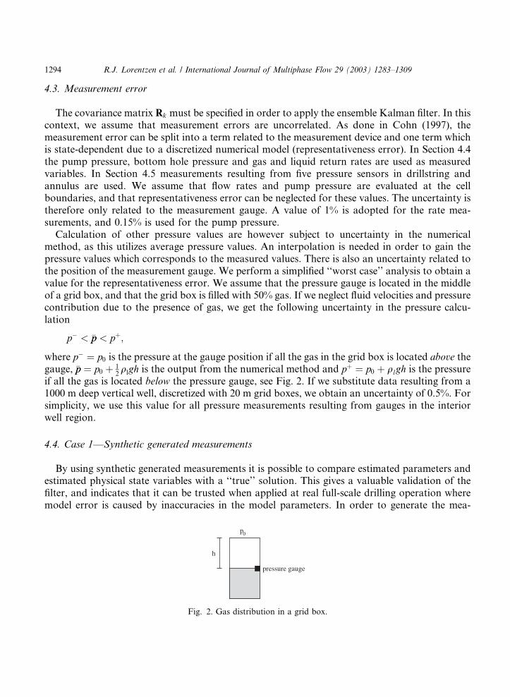
Calculation of other pressure values are however subject to uncertainty in the numericalmethod, as this utilizes average pressure values. An interpolation is needed in order to gain thepressure values which corresponds to the measured values. There is also an uncertainty related tothe position of the measurement gauge. We perform a simplified ‘‘worst case’’ analysis to obtain avalue for the representativeness error. We assume that the pressure gauge is located in the middleof a grid box, and that the grid box is filled with 50% gas. If we neglect fluid velocities and pressurecontribution due to the presence of gas, we get the following uncertainty in the pressure calcu-lation

p� < �pp < pþ;

where p� ¼ p0 is the pressure at the gauge position if all the gas in the grid box is located above thegauge, �pp ¼ p0 þ 1

2qlgh is the output from the numerical method and pþ ¼ p0 þ qlgh is the pressure

if all the gas is located below the pressure gauge, see Fig. 2. If we substitute data resulting from a1000 m deep vertical well, discretized with 20 m grid boxes, we obtain an uncertainty of 0.5%. Forsimplicity, we use this value for all pressure measurements resulting from gauges in the interiorwell region.

4.4. Case 1––Synthetic generated measurements

By using synthetic generated measurements it is possible to compare estimated parameters andestimated physical state variables with a ‘‘true’’ solution. This gives a valuable validation of thefilter, and indicates that it can be trusted when applied at real full-scale drilling operation wheremodel error is caused by inaccuracies in the model parameters. In order to generate the mea-

Fig. 2. Gas distribution in a grid box.


surements, the numerical method described in Section 2.3 is used to calculate a true state vectorWt

k according to the equations

Fig. 3

filter i

Wtk ¼ fðWt

k�1Þ þfemkemk
and
Wt0 ¼ Wt

0 þfem0em0 : ð12Þ
Eq. (10) is then used to calculate synthetic measurements representing pump pressure, bottom
hole pressure and gas and liquid return rates. In this context, we use Wt0 ¼ Wa

0. The error terms femkemkand fem0em0 are assumed to have the same distribution as emk;i and em0;i, but possibly different correlation

factorsfqQijqQij and

gqQ0ijqQ0ij . In order to investigate the importance of these correlation factors, we show

one example (Section 4.4.1) where measurements are generated by using the same correlation

factors as in the Kalman filter equations (8) and (9), and one example (Section 4.4.2) wherefqQijqQij

andgqQ0ijqQ0ij are randomly distributed between 0 and 1. The motivation for adding stochastic noise to

the true parameter values is to simulate external time varying effects caused by the surroundingenvironments and drilling equipment (e.g. change of fluid properties, flow variations and tem-perature variations). In both examples, we have chosen to run the simulator for 80 min, andsample the measurements every 60 s.

Based on experience, a value of 0.2 is chosen as initial standard deviation (rQ0i ) for all pa-

rameters. A value of 5 · 10�3 is used as the accumulating error term (rQi ). Note that this value

depends upon how often the measurements are sampled.We have chosen a dynamic test scenario where gas and liquid are injected (unloading) in two

steps. The well configuration consists of a 1000 m deep vertical drillstring with a 6.03· 10�2 minner diameter, and an annulus with inner diameter equal to 8.89· 10�2 m, and outer diameterequal to 1.59· 10�1 m. The well is initially at rest and filled with water. Flow rates are increased to4.25 Sm3/min for gas and 400 l/min for liquid during a 60 s period. These rates are then keptconstant in 40 min. The injection of gas in the drillstring causes the pump pressure to increasesharply, see the dashed curve in Fig. 3. At approximately 10 min gas enters the annulus and causes

(a) (b)

. The figure shows the pressure measurements in example 1, along with estimated data and a solution where the

s not applied. (a) Pump pressue, (b) bottom hole pressure.


the bottom hole pressure to decrease. The gas front reaches the surface after approximately 25min. At 40 min a new 60 s injection period starts, where the gas and liquid rates are doubled. Theincrease in mass rates generates higher frictional pressure loss. This results in a sudden increase inthe pump pressure and the bottom hole pressure. At approximately 50 min a new gas frontreaches the outlet.

4.4.1. Example 1––equal correlation

In this example the parameter correlation used to generate measurements is the same as in the

Eqs. (8) and (9), that isfqQijqQij ¼ qQ

ij andgqQ0ijqQ0ij ¼ qQ0

ij . Eq. (12) is used to generate an initial true state,and in this case the resulting initial parameter vector is 1

1 M

is det

pt0 ¼ 0:80 �0:30 0:82 0:88 0:83 0:75 1:08 0:81 0:76½ �:

Figs. 3 and 4 show the measurements, the filtered solution and a solution where the filter is notapplied. The non-filtered solution generated with pa0, gives a solution which is different from themeasurements, and spurious gas breakthrough and pressure values are calculated. This indicatesthe importance and need of accurate estimates of the parameter values. As the solid line indicates,the ensemble Kalman filter updates the well flow variables and better agreement with the mea-surements is obtained.

As the measurements are generated synthetically, it is possible to compare estimated and trueflow variables which are not directly measured. Fig. 5 shows the estimated and true gas fraction at500 m below sea surface in the drillstring and annulus. The figure shows good agreement betweenthe estimated and true gas fraction, and indicates that the filter gives a good overall estimate of thewell flow. As we will show below, the updated solution will to some degree remain in its new track,due to a simultaneous update of the parameter vector.

Figs. 6–8 show the evolution of parameter values. Note that the initial estimated parame-ters deviate slightly from their mean values pa0, as they result from the mean of the initial (finitesized) ensemble. The initial leap towards the true parameter values is due to the initial model errorwhich has a larger standard deviation than the accumulating error term. This causes the filter totrust the model less, and measurements more. An improvement in C0;b and C0;s is observed atapproximately 30 min, see Figs. 7 and 8. At this time gas reaches the outlet where it is highlysensitive to variations in the model parameters. This causes the error covariance matrix for theforecasted state to increase, and the model will again be trusted less. In addition, the flow patternbecomes more complex as a transition regime and a slug flow regime are introduced at approx-imately 30 min, see Fig. 9. The estimation of the slug flow parameters has prior to this time beenupdated solely based upon the parameter correlations. The introduction of the transition and slugflow regime is due to increased presence of gas in annulus, which leads to a coalescence of the gasbubbles.

The filter will continuously exert to produce the best overall solution. This implies that the flowvariables with the largest deviation from the measurements are improved, while possibly sacri-

ATLABe�s randn-function is used, which produces quasi-random numbers. The sequence of numbers generated

ermined by the state of the generator. By storing this state, the numbers can be reproduced.

Fig. 4. The figure shows the rate measurements in example 1, along with estimated data and a solution where the filter

is not applied. (a) Gas return rate, (b) liquid return rate.

Fig. 5. True and estimated void fraction in example 1 at two different positions in the well.


ficing accuracy where the error is small. This is achieved by updating the parameters which havethe largest influence on the solution. In the process of estimating the governing parameters, othersmight be withdrawn from their optimal value due to the correlation which exists between theparameters. This is probably the case for C1;d which tends to drift away as C0;b and C0;s approachtheir true values, see Fig. 6.

As the governing parameters approach the corresponding true values one can also expect theforecasted solution to better represent the measured data. We perform a forecast at 5 min, whichillustrates the quality of the estimated solution when only a few measurements are taken intoaccount. In addition, a forecast is performed at 30 min, which is prior to the dynamic behaviorresulting from the second increase in the gas flow rate. Figs. 10 and 11 show the forecasts at these

Fig. 6. Drillstring parameters in example 1. The dashed line represents the true value and the solid line represents the

estimated value.

Fig. 7. Bubble flow parameters in example 1. The dashed line represents the true value and the solid line represents the

estimated value.


moments. As the parameters are quickly improved due to the initial model error, the forecastsolution starting from 5 min gives a considerable improvement when compared to the non-filteredsolution. The pressure levels after the second injection are however underestimated, and the gasbreakthrough is slightly displaced. The forecast starting from 30 min has reduced the deviation inthe bottom hole pressure, and we believe this is due to a better estimate of C0;s, see Fig. 8. Theincrease of this parameter has probably also caused an increase of parameter C1;d , which results ina slightly overestimated pump pressure, see Fig. 10. The overall estimate is however improvedcompared to the forecast starting from 5 min.

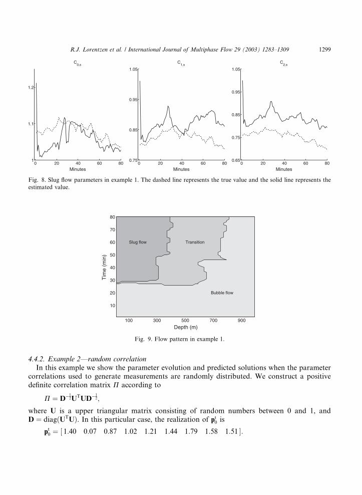
Fig. 8. Slug flow parameters in example 1. The dashed line represents the true value and the solid line represents the

estimated value.

Fig. 9. Flow pattern in example 1.


4.4.2. Example 2––random correlation

In this example we show the parameter evolution and predicted solutions when the parametercorrelations used to generate measurements are randomly distributed. We construct a positivedefinite correlation matrix P according to

P ¼ D�12UTUD�1

2;

where U is a upper triangular matrix consisting of random numbers between 0 and 1, andD ¼ diagðUTUÞ. In this particular case, the realization of pt0 is

pt0 ¼ 1:40 0:07 0:87 1:02 1:21 1:44 1:79 1:58 1:51½ �:

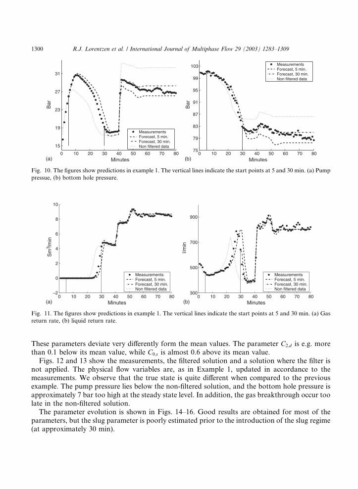
Fig. 10. The figures show predictions in example 1. The vertical lines indicate the start points at 5 and 30 min. (a) Pump

pressue, (b) bottom hole pressure.

Fig. 11. The figures show predictions in example 1. The vertical lines indicate the start points at 5 and 30 min. (a) Gas

return rate, (b) liquid return rate.


These parameters deviate very differently form the mean values. The parameter C2;d is e.g. morethan 0.1 below its mean value, while C0;s is almost 0.6 above its mean value.

Figs. 12 and 13 show the measurements, the filtered solution and a solution where the filter isnot applied. The physical flow variables are, as in Example 1, updated in accordance to themeasurements. We observe that the true state is quite different when compared to the previousexample. The pump pressure lies below the non-filtered solution, and the bottom hole pressure isapproximately 7 bar too high at the steady state level. In addition, the gas breakthrough occur toolate in the non-filtered solution.

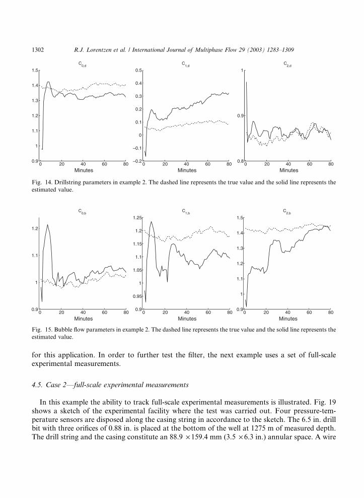
The parameter evolution is shown in Figs. 14–16. Good results are obtained for most of theparameters, but the slug parameter is poorly estimated prior to the introduction of the slug regime(at approximately 30 min).

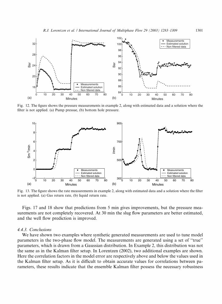
Fig. 12. The figure shows the pressure measurements in example 2, along with estimated data and a solution where the

filter is not applied. (a) Pump pressue, (b) bottom hole pressure.

Fig. 13. The figure shows the rate measurements in example 2, along with estimated data and a solution where the filter

is not applied. (a) Gas return rate, (b) liquid return rate.


Figs. 17 and 18 show that predictions from 5 min gives improvements, but the pressure mea-surements are not completely recovered. At 30 min the slug flow parameters are better estimated,and the well flow prediction is improved.

4.4.3. ConclusionsWe have shown two examples where synthetic generated measurements are used to tune model

parameters in the two-phase flow model. The measurements are generated using a set of ‘‘true’’parameters, which is drawn from a Gaussian distribution. In Example 2, this distribution was notthe same as in the Kalman filter setup. In Lorentzen (2002), two additional examples are shown.Here the correlation factors in the model error are respectively above and below the values used inthe Kalman filter setup. As it is difficult to obtain accurate values for correlations between pa-rameters, these results indicate that the ensemble Kalman filter possess the necessary robustness

0 20 40 60 800.9

1

1.1

1.2

1.3

1.4

1.5

Minutes

C0,d

0 20 40 60 80–0.2

–0.1

0

0.1

0.2

0.3

0.4

0.5

Minutes

C1,d

0 20 40 60 800.8

0.9

1

Minutes

C2,d

Fig. 14. Drillstring parameters in example 2. The dashed line represents the true value and the solid line represents the

estimated value.

Fig. 15. Bubble flow parameters in example 2. The dashed line represents the true value and the solid line represents the

estimated value.


for this application. In order to further test the filter, the next example uses a set of full-scaleexperimental measurements.

4.5. Case 2––full-scale experimental measurements

In this example the ability to track full-scale experimental measurements is illustrated. Fig. 19shows a sketch of the experimental facility where the test was carried out. Four pressure-tem-perature sensors are disposed along the casing string in accordance to the sketch. The 6.5 in. drillbit with three orifices of 0.88 in. is placed at the bottom of the well at 1275 m of measured depth.The drill string and the casing constitute an 88.9 · 159.4 mm (3.5 · 6.3 in.) annular space. A wire

Fig. 16. Slug flow parameters in example 2. The dashed line represents the true value and the solid line represents the

estimated value.

Fig. 17. The figures show predictions in example 2. The vertical lines indicate the start points at 5 and 30 min. (a) Pump

pressue, (b) bottom hole pressure.


line logging tool is monitoring real time pressure and temperature in the drillstring at 490 m. Inthis context, the temperature measurements are neglected, and pressure measurements from foursensors in annulus and one sensor in drillstring are used. The measurements are sampled every60 s, and a period of 180 min is simulated. The effect of variations in the sampling rate and re-duction of available sensors are discussed in Lorentzen (2002).

In this example we have used 5· 10�4 as standard deviation for the accumulating model error(rQ

i ). A value of 1.5· 10�3 is adopted as initial standard deviation (rQ0i ). These values should

reflect presumed uncertainty in the model parameters. It was however found necessary to restrictthe standard deviations to some degree, to prevent too radical changes in the parameters from one

Fig. 18. The figures show predictions in example 2. The vertical lines indicate the start points at 5 and 30 min. (a) Gas

return rate, (b) liquid return rate.

Fig. 19. Well configuration for the test facility.


time step to the next. If this happened, we experienced breakdowns in the simulator in periodswhere the flow is highly dynamic.

The tests start with the well at rest and filled with water, and the flow rates are increased to 7.6Sm3/min and 605.5 l/min for gas and liquid respectively. The injection of gas in the drillstringcauses the pump pressure to increase sharply. At approximately 20 min the gas enters the annulusand causes the bottom hole pressure to decrease, see Fig. 24. The pressure sensors detect thepresence of gas as the gas phase reaches their positions. After approximately 50 min of injection,the gas flow rate is adjusted to 15.2 Sm3/min, while the liquid injection is kept at a constant rate.The increased presence of gas causes the bottom hole pressure to decrease with time. After 140min, the gas rate is further increased to 25.4 Sm3/min.


Figs. 20–22 show the measurements, the filtered solution and a solution where the filter is notapplied. The model error is reduced when compared to Case 1, and the estimated solution is notfollowing the measurements with the same accuracy as in that case. Improvements are howeverseen from approximately 30 min. As can be seen from the figures, the model is over-predicting thepressure throughout the well, and the (important) bottom hole pressure has at the most an errorof 15 bar. The aim of applying the filter is to estimate parameters with higher validity for this wellscenario, and thereby obtain more accurate forecasts of the flow.

The measurements show some pressure variations which are not present in the forecast solution(e.g. in the drillstring at approximately 100 min). These variations are due to complex chokeconstrains in the experimental facility, and these constrains are not included in the physical modelused here. The focus in this case is therefore to capture the main tendencies of the two-phase flow.

Fig. 20. The figure shows estimation of the drillstring pressure at 490 m. The measurements and an initial prediction are

also shown.

Fig. 21. The figures show estimations of the bottom hole pressure and the annulus pressure at 998 m. The measure-

ments and an initial prediction are also shown. (a) Bottom hole pressure, (b) annulus pressure at 998 m.

(a) (b)

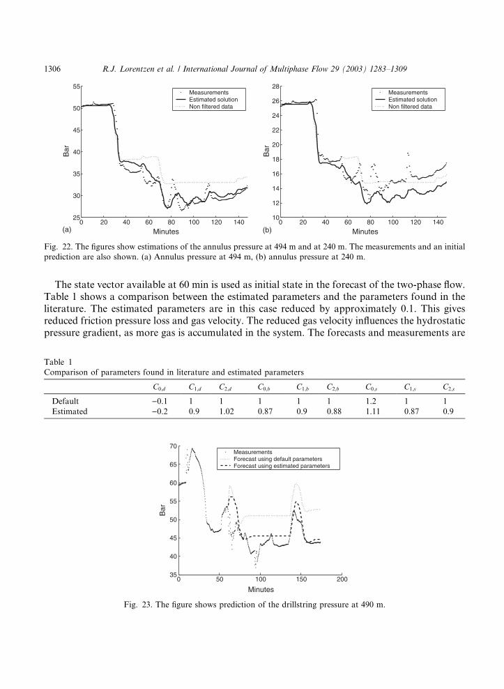
Fig. 22. The figures show estimations of the annulus pressure at 494 m and at 240 m. The measurements and an initial

prediction are also shown. (a) Annulus pressure at 494 m, (b) annulus pressure at 240 m.


The state vector available at 60 min is used as initial state in the forecast of the two-phase flow.Table 1 shows a comparison between the estimated parameters and the parameters found in theliterature. The estimated parameters are in this case reduced by approximately 0.1. This givesreduced friction pressure loss and gas velocity. The reduced gas velocity influences the hydrostaticpressure gradient, as more gas is accumulated in the system. The forecasts and measurements are

Table 1

Comparison of parameters found in literature and estimated parameters

C0;d C1;d C2;d C0;b C1;b C2;b C0;s C1;s C2;s

Default )0.1 1 1 1 1 1 1.2 1 1

Estimated )0.2 0.9 1.02 0.87 0.9 0.88 1.11 0.87 0.9

Fig. 23. The figure shows prediction of the drillstring pressure at 490 m.

Fig. 24. The figures show predictions of the bottom hole pressure and the annulus pressure at 998 m. (a) Bottom hole

pressure, (b) annulus pressure at 998 m.

Fig. 25. The figures show predictions of the annulus pressure at 494 m and at 240 m. (a) Annulus pressure at 494 m,

(b) annulus pressure at 240 m.


shown in Figs. 23–25. The figures also show a forecast where the estimated physical variables (v) isused as an initial condition, but the default parameters are still kept. This forecast shows that is iscrucial to update the model parameters, as the well flow in this case quickly approaches thesolution obtain without the filter (compare with the non-filtered data shown in Figs. 20–22).The forecast using estimated parameters show large improvements at the sensor position in thedrillstring and at the two deepest positions in the annulus. At the positions close to the outlet,the predictions are drifting away from the optimal track. This is due to the fact that largestdifference between model and measurements occur at positions where the pressure is high.Measurements at these positions does therefore obtain a larger weight in the Kalman filterequations, and parameters are tuned so that better agreement is achieved. Accurate prediction ofthe bottom hole pressure is however considered to be of particular interest during several oper-ations related to drilling and production.


5. Summary and conclusions

A new approach of tuning of parameters in two-phase flow models is presented. The approachuses an ensemble Kalman filter in the tuning. Motivated by applications in underbalanceddrilling, the modeling of two-phase flow in wells is outlined and the implementation of the en-semble Kalman filter is presented. We have shown one way of including model parameters in thefilter and present two studies of the suggested approach.

First, we study the robustness of the method using synthetic data. Synthetic measurements aregenerated by running the simulator using different sets of model parameters. Although the modelparameters are not correctly recovered, the filter produce solutions which fits the observations andgive improved forecasts compared to using the standard choice of model parameters. As this holdsfor different choices of ‘‘true’’ model parameters, this leads us to conclude that the ensembleKalman filter approach has necessary robustness properties for this application.

The second study applies the suggested approach to experimental data. It is shown that tuningthe chosen model parameters gives a solution which improved fitting of the measurements, andthe forecast is significantly better than the solution obtained without the filter. Still there are somebehavior of the flow which the filter is not able to track. This points to the fact that there arechallenges ahead both on the modeling of the process and in the use of the Kalman filter tech-niques for online model parameter tuning.

Acknowledgements

We thank the Norwegian Research Council for financial support through the Strategic InstituteProgram ‘‘Complex Wells’’. We also thank our colleagues at RF-Rogaland Research, ErlendH. Vefring, Kjell K. Fjelde, Ove Sævareid and Johnny Frøyen, for useful discussions.

References

Anderson, J.L., 2001. An ensemble adjustment Kalman filter for data assimilation. Monthly Weather Rev. 129, 2884–

2903.

Bendiksen, K., 1984. An experimental investigation of the motion of long bubbles in inclined tubes. Int. J. Multiphase

Flow 10, 467–483.

Bendiksen, K., Malnes, D., Moe, R., Nuland, S., 1991. The dynamic two-fluid model OLGA: Theory and application.

SPE Production Engineering.

Bendiksen, K.H., Malnes, D., Nydal, O.J., 1996. On the modelling of slug flow. Chem. Eng. Comm. 141–142, 71–102.

Burgers, G., van Leeuwen, P.J., Evensen, G., 1998. On the analysis scheme in the ensemble Kalman filter. Mon.

Weather Rev. 126, 1719–1724.

Cassaude, B., Fabre, J., Jean, C., Ozon, P., Theron, B., June 1989. Unsteady phenomena in horizontal gas–liquid slug

flow. In: Proceedings of the 4th International Conference on Multi-phase Flow. Nice, France, Cranfield, BHRA ,

pp. 469–484.

Cohn, S.E., 1997. An introduction to estimation theory. J. Meteorolog. Soc. Jpn. 75, 257–288.

Evensen, G., 1994. Sequential data assimilation with a nonlinear quasi-geostrophic model using Monte Carlo methods

to forecast error statistics. J. Geophys. Res. 99, 10143–10162.

Faille, I., Heintz�ee, E., 1999. A rough finite volume scheme for modeling two-phase flow in a pipeline. Computers &

Fluids, 213–241.


Fjelde, K.K., 2000. Numerical schemes for complex nonlinear hyperbolic systems of equations. Ph.D. thesis,

Department of Mathematics, University of Bergen.

Franca, F., Lahey, R., 1992. The use of drift-flux techniques for the analysis of horizontal 2-phase flows. Int. J.

Multiphase Flow 18, 787–801.

Frøyen, J., Sævareid, O., Vefring, E.H., 2000. Discretization, implementation and testing of a semi-implicit method.

Tech. rep., RF–– Rogaland Research, confidential.

Gavage, S.B., 1991. Analyse num�eerique des mod�eeles hydrodynamiques d��eecoulements diphasiques instationnaires dans

les r�eeseaux de production p�eetroli�eere. Th�eese, ENS Lyon France.

Hamil, T.M., Whitaker, J.S., Snyder, C., 2001. Distance-dependent filtering of background error covariance estimates

in an ensemble Kalman filter. Monthly Weather Rev. 129, 2776–2790.

Harmathy, T., 1960. Velocity of large drops and bubbles in media of infinite or restricted extent. AIChE J. 6, 281–288.

Houtekamer, P.L., Mitchell, H.L., 1998. Data assimilation using an ensemble Kalman filter technique. Monthly

Weather Rev. 126, 796–811.

Ishii, M., 1975. Thermo-Fluid Dynamic Theory of Two-Phase Flow. Eyrolles, Paris.

Kelessidis, V., Dukler, A., 1989. Modeling flow pattern transitions for upward gas–liquid flow in vertical concentric and

eccentric annuli. Int. J. Multiphase Flow 15, 173–191.

Lage, A.C.V.M., 2000. Two-phase flow models and experiments for low-head and underbalanced drilling. Ph.D. thesis,

Stavanger University College, Norway.

Lage, A.C.V.M., Time, R.W., October 2000. Mechanistic model for upward two-phase flow in annuli. In: The 2000 SPE

Annual and Technical Conference and Exhibition. Dallas, Texas, SPE 63127.

Lage, A.C.V.M., Fjelde, K.K., Time, R.W., September 2000a. Underbalanced drilling dynamics: Two-phase flow

modeling and experiments. In: The 2000 IADC/SPE Asia Pacific Drilling Technology. Kuala Lumpur, Malaysia,

IADC/SPE 62743.

Lage, A.C.V.M., Frøyen, J., Sævareid, O., Fjelde, K.K., October 2000b. Underbalanced drilling dynamics: Two-phase

flow modeling, experiments and numerical solution techniques. In: The Rio Oil & Gas Conference. Rio de Janerio,

Brazil, IBP 41400.

Lorentzen, R.J., April 2002. Higher order numerical methods and use of estimation techniques to improve modeling of

two-phase flow in pipelines and wells. Ph.D. thesis, Department of Mathematics, University of Bergen.

Lorentzen, R.J., Fjelde, K.K., Frøyen, J., Lage, A.C.V.M., Nævdal, G., Vefring, E.H., 30 September–3 October 2001a.

Underbalanced and low-head drilling operations: Real time interpretation of measured data and operational

support. In: 2001 SPE Annual Technical Conference and Exhibition. SPE 71384.

Lorentzen, R.J., Fjelde, K.K., Frøyen, J., Lage, A.C.V.M., Nævdal, G., Vefring, E.H., 27 February–1 March 2001b.

Underbalanced drilling: Real time data interpretation and decision support. In: SPE/IADC Drilling Conference.

Amsterdam, The Netherlands, SPE/IADC 67693.

Maybeck, P.S., 1979. In: Stochastic models, estimation, and control, Vol. 1. Academic Press, New York.

Nævdal, G., Mannseth, T., Vefring, E.H., 3–6 September 2002a. Instrumented wells and near-well reservoir monitoring

through ensemble Kalman filter. In: Proceedings of 8th European Conference on the Mathematics of Oil Recovery.

Freiberg, Germany.

Nævdal, G., Mannseth, T., Vefring, E.H., April 2002b. Near-well reservoir monitoring through ensemble Kalman filter.

In: SPE/DOE Improved Oil Recovery Symposium. Tulsa, Oklahoma, SPE 75235.

Papadimitriou, D., Shoham, O., April 1991. A mechanistic model for predicting annulus bottomhole pressures in

pumping wells. In: 1991 Production Operations Symposium. Oklahoma City, SPE 21669.

Pauchon, C.L., Dhulesia, H., Binh-Cirlot, G., Fabre, J., September 1994. Tacite: A transient tool for multiphase

pipeline and well simulation. In: The 1994 SPE Annual and Technical Conference and Exhibition. New Orleans, LA,

SPE 28545.

Taitel, Y., Barnea, D., 1983. Counter current gas–liquid vertical flow, model for flow pattern and pressure drop. Int. J.

Multiphase Flow 9, 637–647.

Th�eeron, B., 1989. Ecoulements diphasique instationnaires en conduite horizontale. Th�eese, INP Toulouse, France.

Verlaan, M., Heemink, A.W., 2001. Nonlinearity in data assimilation applications: A practical method for analysis.

Monthly Weather Rev. 129, 1578–1589.

Wallis, G., 1969. One Dimensional Two-Phase Flow. McGraw-Hill Book Co. Inc.

multiphase enkf

Documents