multidimensional signalling -...

Journal of Mathematical Economics 14 (1985) 261-284. North-Holland

MULTIDIMENSIONAL SIGNALLING

Martine QUINZII

Laboratoire d’Economttrie de I’Ecole Polytechnique and Universit6 Paris II, Paris, France

Jean-Charles ROCHET*

Ecole Polytechnique and CEREMADE, Universik Paris IX, Paris, France

Received November 1985

Spence’s model of market signalling is extended to the case of multidimensional characteristics. Assuming separable costs, we give a characterization of equilibria as related to the convex solutions of some partial differential equation. An existence result is obtained under an additional assumption, which was not needed in dimension one.

1. Introduction

Many recent papers have emphasized the importance of informational asymmetries in the functioning of markets. Since the pioneering article of Akerlof (1970), it has been recognized that, in some cases, they can preclude mutually profitable exchanges between buyers and sellers.

Spence (1973, 1974) introduced the idea that market signalling can partly remedy to this imperfection. Spence considered mainly the example of the labor market, for which he defined, in the competitive case, the notion of signalling equilibrium. Riley (1979) extended the model so as to deal with more general contexts of asymmetric information than the labor market. In all this work, there is a one dimensional parameter which is unknown of one side of the market and information goes through a one dimensional signal. Under natural conditions, there exists a one parameter family of equilibria, all ranked by the Pareto criterion.

It was more or less implicitly assumed that generalization of these results to a more realistic case of manifold uncertainty would be straightforward. However Kohlleppel (1983) exhibited an example of a two dimensional extension of the model of Spence for which no equilibrium exists.

The purpose of this paper is to clarify the qualitative difference between one and several dimensions. The analysis is restricted to a multidimensional

*We are indebted to Martin Hellwig, Lauren2 Kohlleppel and especially Jean-Michel Lasry for their helpful comments. All remaining errors are of course our own responsibility.

03044068/85/$3.30 0 198.5, Elsevier Science Publishers B.V. (North-Holland)

262 M. Quinzii and J.-C. Rochet, Multidimensional signalling

generalization of the Spence’s model of labor market. In section 2 we present the model and the notion of equilibrium that we study. In a signalling equilibrium, agents of different productivity are sorted out by the signals they choose. In section 3 we analyze the cause of inexistence of equilibrium in Kohlleppel’s counterexample: the second order condition of the workers’ maximization problem cannot be fulfilled in a separating equilibrium. In section 4 we provide, in the case of separable costs, a simple characterization of signalling equilibria in terms of convex solutions to some partial differential equation. An existence result is given in section 5 with an additional assumption which was not needed in dimension 1. We also prove that the same assumption implies that separating equilibrium is the only form of equilibrium compatible with Nash-Bertrand competition on the firms’ side. Finally section 6 discusses the ‘pure signalling’ case in which the signal is not productive. A counter example is given which shows that, even with separable costs and improductive signals, an additional assumption is necessary to obtain existence of equilibrium in the case of multiple dimensions.

2. The model

We will use a straightforward extension of the one dimensional partial equilibrium model of labor market proposed by Spence (1973,1974). The sellers’ side is represented by a continuum of workers, selling their labor to a set of competitive firms. The crucial feature of the market is the asymmetry of information between buyers and sellers. The productivity of an individual at work (therefore the quality of the good he or she sells) depends on innate ‘characteristics’ of this individual which are unobservable by the employers prior to hiring. Even if these ‘characteristics’ are difticult to define precisely, it seems clear that in many cases they are manifold, and thus impossible to subsume in a unique index. Consequently we will represent these characteristics by a k-dimensional vector n=(ni, . . . , Q). The set of all possible characteristics is a subset N of R:.

The second determinant of a worker’s productivity is a vector Y=

(Y i,.“, yh) of observable and alterable attributes (essentially educational performances). Investment in education serves as a signal upon which employers make evaluations about individual productivities. The set of possible signals will be all Rt.

In the following, when we refer to the one dimensional model, we refer to the case where h = k = 1.

Except for the possibility of multidimensional characteristics and signals, we make the same simplifying assumptions as Spence:

_ the firms are all the same in the sense that agents have the same productivity in each firm,

M. Quinzii and J.-C. Rochet, Multidimensional signalling 263

- the technology has constant returns to scale so that a firm’s output is the sum of individual products of all workers in this firm.

We can then speak of the productivity s(n, y) of an agent of characteristics n choosing signals y. For such an agent, signalling costs are, in monetary units, c(n, y).

Since all the firms are the same and employers can observe only the signals, we will study symmetric situations where all firms propose the same wage schedule based on the observable signals. This wage schedule will be denoted w(y).

We assume that an agent of characteristics n, given the wage schedule w(a), selects a signal y(n) so as to maximize his or her net income

W(Y) - 4% Y).

We would like to prove existence of symmetric Nash equilibria of this market where an infinite number of potential firms compete through the wage schedule that they offer to the workers.

Unfortunately Riley (1979) has shown that, even in the one dimensional model Nash equilibria need not exist.

What always exists in dimension one under natural conditions is an equilibrium where

- firms make zero profits, _ individuals are completely sorted out by the signal in the sense that agents

of different characteristics choose different levels of signal.

These two conditions can be summarized in the relation

dY(4) = sh Y(4). (2.1)

It is clear that, in one or multidimensions, free entry of potential firms in the market drive profits to zero.

In dimension one, one can prove [Riley (1979)] that only separating equilibria are compatible with competition among firms. If agents of different abilities were induced to choose the same signal j, they would all receive the same wage w(j) equal to their average productivity. A firm could enter and propose a wage w(Y) +E to the workers choosing signal Y+ a, zero to the others. E and a can be chosen such as to attract only the more able workers in the ‘pool’ and make a profit.

In the multidimensional case, this reasoning does not hold because characteristics can no longer be linearly ordered. Pooling equilibria cannot be disregarded in higher dimensions for the reason that they are unstable under the pressure of competition.


Definition. A signalling equilibrium is a pair of functions

w: rw:+rw+,

y: N+[W: such that, for all n in N:

(a) y(n) maximizes {w(y) - c(n, y)> over R:,

V-4 wdv(4) = shy(n)).

Existence of signalling equilibria has been proved, in the one dimensional case (k = h = l), by Spence (1973,1974) under the following assumptions:

(a.]) N = [n, ?I],

(a.2) c and s are twice continuously differentiable,

(a.3) (a2c/~y dn)(y, n) < 0 for all (y, n),

(a.4) (W~Y)(Y, 4 > 0, (WW(y, n) > 0, (Way)(y, 4 2 0 for all (Y, 4,

(~3) total surplus [s(n, y)-c(n, y)] is a concave function of y having, for all n, a maximum on R + .

While (a.1) and (a.2) are technical assumptions, and (a.4), (a.5) express natural conditions on (y, n), the crucial assumption is (a.3). In order for education to be used as a proxy for natural ability n, marginal cost of education has to be a decreasing function of n. On more technical grounds, Spence proved that signalling equilibria could be identified with a one parameter family of solutions to a certain ordinary differential equation. Moreover these equilibria can be ranked by the Pareto criterion.

As told earlier, Riley (1975,1979) studied the stability of these equilibria to competitive behaviour of firms. He proved that, if none of them is a Nash equilibrium, the Pareto superior one is stable in a weaker sense. It can be

M. Quinzii and J.-C. Rochet, Multidimensional signding 265

supported as a ‘reactive equilibrium’ where firms do not deviate if they anticipate that their profitable deviations can raise reactions from the other firms which can lead them finally to suffer losses.

One could conjecture, and indeed this was more or less implicit in the papers of Spence and Riley, that the existence results could be easily adapted to the case of multiple characteristics, under a natural extension of assumptions (a.1) to (a.5). However, Kohlleppel (1983) gave an example of non- existence of equilibrium for h = k = 2. Kohlleppel’s counterexample, which we study in section 3, shows that there are qualitative differences between models with one dimensional uncertainty and more general models with manifold uncertainties. This point was also made clear in a different context by Baron-Myerson (1982).

3. Kohlleppel’s counter-example

In order to get some insight of the differences between one and several characteristics, let us briefly recall Kohlleppel’s counter-example. This will help to identify the cause of inexistence of an equilibrium. The cost and productivity functions are given by

shy)=n,, (3.1)

c(n 7 y)-y’ f y:+y:

9

n2 n1n2 (3.2)

where n=(ni, n2) belongs to a compact subset N of rW: + and y =(yi, y2) is a vector of rW:. It is easy to see that these functions fulfill the natural extensions of assumptions (a.l)<aS) to the several dimensions case. For instance, it is easy to check that

&(n, y) ~0 for all i,j and (n, y). 1 J

Eq. (3.1) shows that we are in a ‘pure signalling’ case. In other words, the signal adds nothing to the productivity of the agents. Eq. (3.2) suggests the change of variables (z,, z2) = (yf + y& y2), that will simplify our computations.

Let 2 = (z E rW:, z1 2 z$> be the set of possible signals and w:Z-+R be a candidate for equilibrium. Assuming differentiability, an interior solution of the program

max w(z)---? i

21 ZEZ n1n2 n2 I

(3.3)

266 M. Quinzii ana’ J.-C. Rochet, Multidimensional signalling

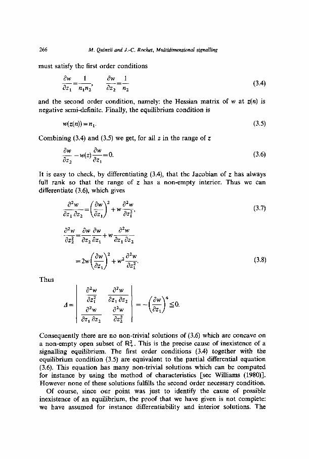
must satisfy the first order conditions

aw I at4 i -- 3g-n&

-=- 82, n2

(3.4)

and the second order condition, namely: the Hessian matrix of w at z(n) is negative semi-definite. Finally, the equilibrium condition is

w(z(n)) =nl.

Combining (3.4) and (3.5) we get, for all z in the range of z

(3.5)

aw - -w(z)g=o. 82, 1

(3.6)

It is easy to check, by differentiating (3.4), that the Jacobian of z has always full rank so that the range of z has a non-empty interior. Thus we can differentiate (3.6), which gives

a2w aw 2 a% ---= - aZ, a2, aZ, + Wq ( ) a2w aw aw a% 2@=aZ,az,+ w az, az2

Thus

A=

=2w g 2+wz$. ( > 1 1

a% a% -___ a$ az, az, ah a2w

aZ,aZ, ( ) aw 4<o =- - aZ, =.

(3.7)

(3.8)

Consequently there are no non-trivial solutions of (3.6) which are concave on a non-empty open subset of W:. This is the precise cause of inexistence of a signalling equilibrium. The first order conditions (3.4) together with the equilibrium condition (3.5) are equivalent to the partial differential equation (3.6). This equation has many non-trivial solutions which can be computed for instance by using the method of characteristics [see Williams (1980)]. However none of these solutions fulfills the second order necessary condition.

Of course, since our point was just to identify the cause of possible inexistence of an equilibrium, the proof that we have given is not complete: we have assumed for instance differentiability and interior solutions. The

M. Quinzii ana’ J.-C. Rochet, Multidimensional signalling 267

reader can find a complete proof not based on differential techniques in Kohlleppel (1983).

4. The case of separable costs: A characterization theorem

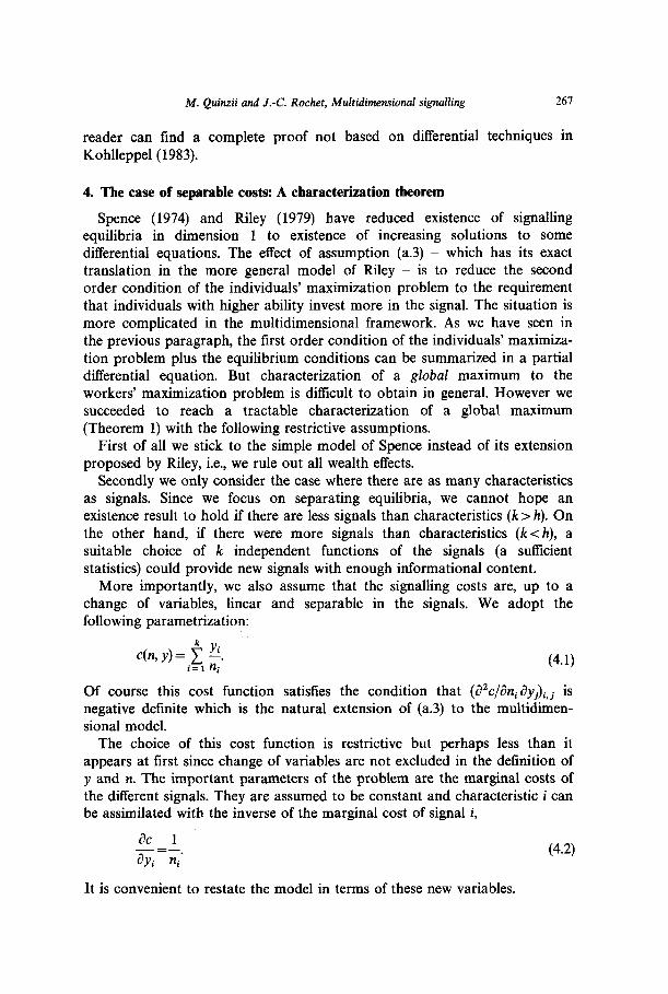
Spence (1974) and Riley (1979) have reduced existence of signalling equilibria in dimension 1 to existence of increasing solutions to some differential equations. The effect of assumption (a.3) - which has its exact translation in the more general model of Riley - is to reduce the second order condition of the individuals’ maximization problem to the requirement that individuals with higher ability invest more in the signal. The situation is more complicated in the multidimensional framework. As we have seen in the previous paragraph, the first order condition of the individuals’ maximization problem plus the equilibrium conditions can be summarized in a partial differential equation. But characterization of a global maximum to the workers’ maximization problem is difficult to obtain in general. However we succeeded to reach a tractable characterization of a global maximum (Theorem 1) with the following restrictive assumptions.

First of all we stick to the simple model of Spence instead of its extension proposed by Riley, i.e., we rule out all wealth effects.

Secondly we only consider the case where there are as many characteristics as signals. Since we focus on separating equilibria, we cannot hope an existence result to hold if there are less signals than characteristics (k>h). On the other hand, if there were more signals than characteristics (k<h), a suitable choice of k independent functions of the signals (a sufficient statistics) could provide new signals with enough informational content.

More importantly, we also assume that the signalling costs are, up to a change of variables, linear and separable in the signals. We adopt the following parametrization:

(4.1)

Of course this cost function satisfies the condition that (J’C/aniayj)i,j is negative definite which is the natural extension of (a.3) to the multidimensional model.

The choice of this cost function is restrictive but perhaps less than it appears at first since change of variables are not excluded in the definition of y and n. The important parameters of the problem are the marginal costs of the different signals. They are assumed to be constant and characteristic i can be assimilated with the inverse of the marginal cost of signal i,

ac i - =-. aYi ni

It is convenient to restate the model in terms of these new variables.

(4.2)


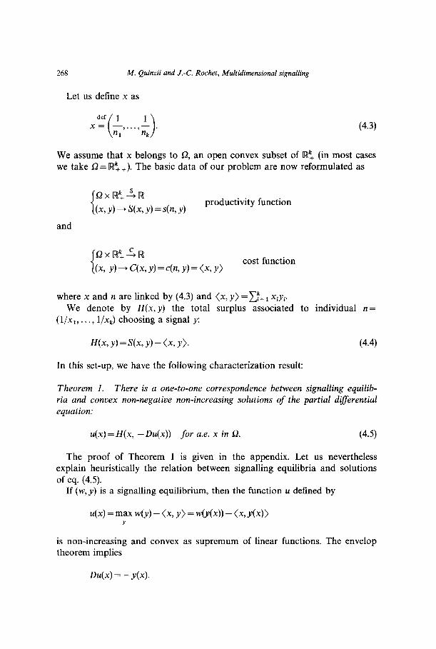
Let us define x as

. (4.3)

We assume that x belongs to 52, an open convex subset of R: (in most cases we take D = lF!$ +). The basic data of our problem are now reformulated as

productivity function

and

i

52x[w:%! (x, Y) - cc? Y) = ch Y) = <x7 Y>

cost function

where x and n are linked by (4.3) and (x, y) =I!= 1 Xiy,. We denote by H(x,y) the total surplus associated

(l/x I,..., l/xk) choosing a signal y:

H(x, Y) = w, Y) - <x, Y>.

to individual n=

(4.4)

In this set-up, we have the following characterization result:

Theorem 1. There is a one-to-one correspondence between signalling equilibria and convex non-negative non-increasing solutions of the partial differential equation:

u(x) = H(x, - Du(x)) for a.e. x in 52. (4.5)

The proof of Theorem 1 is given in the appendix. Let us nevertheless explain heuristically the relation between signalling equilibria and solutions of eq. (4.5).

If (w, y) is a signalling equilibrium, then the function u defined by

44 = max W(Y) - <A Y > = 4.W) - <x9 Y(x)> Y

is non-increasing and convex as supremum of linear functions. The envelop theorem implies

h(x) = -y(x).


The equilibrium conditions w@(x)) = S(x, y(x)) then implies that u satisfies eq. (4.5).

The proof of Theorem 1 essentially consists in showing that the converse holds. If (4.5) has a convex non-increasing solution u then

4.w) = 44 - (x, Mx)), y(x) = - Du(x)

define almost everywhere a signalling equilibrium.

5. An existence result

Theorem 1 provides us, in the case of linear separable costs, with a convenient characterization of signalling equilibria. An equilibrium exists if and only if there exists at least one convex non-negative non-increasing solution to eq. (4.5):

u(x) = H(x, -&J(X)) for a.e. x in Sz. (4.5)

In fact, equations like (4.5) are well known in optimal control theory and variations calculus. Under certain assumptions one can obtain explicit solutions to equations like (4.5) as value functions of a well-chosen calculus of variations problem. Let us set, for x in Q and 4 in IWk

ff*c% 4) = sup {H(x, Y) + (4, Y>>. YERf

(5.1)

H*(x, .) is the conjugate function of -H(x, .) [Rockafellar (1970, p. 104)]. We set

$4 = ccEf,x ‘{ e-‘H*(t(O, 80) dt), (5.2)

where

%={5Eg(R+,Q)/[. is continuous except on a finite set

and c(O) = x}. (5.3)

%‘X is, as usual in control theory, a set of trajectories starting from x, remaining in 52 for all t, and having only a finite number of kinks. H* being continuous in (x,q) on the interior of its domain, the integral in (5.2) is well defined. In fact we will prove that as soon as (5.2) defines a finite number for all x in C?, U(x) is a solution to eq. (4.5). The following theorem gives sufficient conditions for U to be a convex solution of (4.5). For simplicity, we will take from now on 52 = rW$ +.


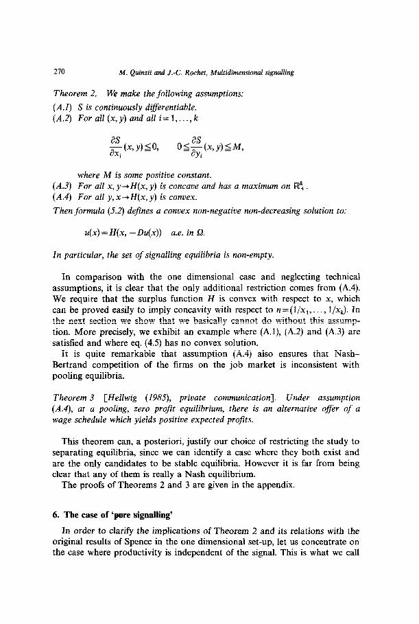
Theorem 2. We make the following assumptions:

(A.1) S is continuously dt@erentiable. (A.2) For all (x, y) and all i= 1,. . . , k

where M is some positive constant. (A.3) For all x, y+H(x, y) is concave and has a maximum on Wt. (A.4) For all y, x-+H(x, y) is convex.

Then formula (5.2) dejnes a convex non-negative non-decreasing solution to:

u(x) = H(x, - Du(x)) a.e. in 52.

In particular, the set of signalling equilibria is non-empty.

In comparison with the one dimensional case and neglecting technical assumptions, it is clear that the only additional restriction comes from (A.4). We require that the surplus function H is convex with respect to x, which can be proved easily to imply concavity with respect to n =( l/x1,. . . , l/xJ. In the next section we show that we basically cannot do without this assumption. More precisely, we exhibit an example where (A.l), (A.2) and (A.3) are satisfied and where eq. (4.5) has no convex solution.

It is quite remarkable that assumption (A.4) also ensures that Nash- Bertrand competition of the firms on the job market is inconsistent with pooling equilibria.

Theorem 3 [Hellwig (198.5), private communication]. Under assumption (A.4), at a pooling, zero profit equilibrium, there is an alternative ofleer of a wage schedule which yields positive expected profits.

This theorem can, a posteriori, justify our choice of restricting the study to separating equilibria, since we can identify a case where they both exist and are the only candidates to be stable equilibria. However it is far from being clear that any of them is really a Nash equilibrium.

The proofs of Theorems 2 and 3 are given in the appendix.

6. The case of ‘pure signalling’

In order to clarify the implications of Theorem 2 and its relations with the original results of Spence in the one dimensional set-up, let us concentrate on the case where productivity is independent of the signal. This is what we call


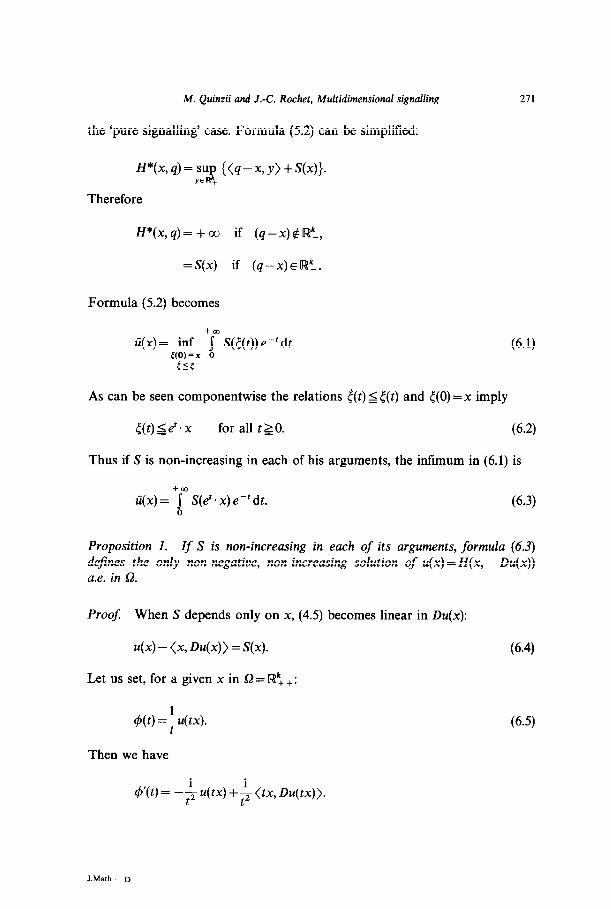
the ‘pure signalling’ case. Formula (5.2) can be simplified:

H*(x, 4) = sup {+I - x, Y> + WI. YER+

Therefore

H*(x,q)= +cc if (q-x)$Rk,

=S(x) if (q-x)ElRk.

Formula (5.2) becomes

U(x) = inf +Jm S({(t)) e-‘dt. C(O)=x 0 rs<

(6.1)

As can be seen componentwise the relations t(t) 5 c(t) and c(O) =x imply

<(t)see’.x for all t?O. (6.2)

Thus if S is non-increasing in each of his arguments, the infimum in (6.1) is

-km U(x)= j S(e’.x)e-‘dt.

0 (6.3)

Proposition 1. Zf S is non-increasing in each of its arguments, formula (6.3) defines the only non-negative, non-increasing solution of u(x) = H(x, -Du(x)) a.e. in Sz.

Proof: When S depends only on x, (4.5) becomes linear in Du(x):

u(x) - (x, h(x)) = S(x).

Let us set, for a given x in s2 = R: + :

(6.4)

4(t) =f u(tx). (6.5)

Then we have

4’(t) = -f u(tx) +$ (tx, Du(tx)).

J.Math- D


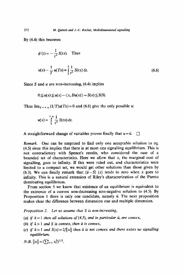
By (6.4) this becomes

4’(t) = - ;S(“x). Thus

u(x) - ; u( TX) = 7 $ S(tx) dt.

Since S and u are non-increasing, (6.4) implies

0 5 u(x) 5 U(X) - (x, Du(x)) = S(x) 5 S(0).

Thus lim,, + m (l/T)u( TX) = 0 and (6.6) give the

u(x) = +im ; S(tx) dt.

(6.6)

only possible u:

A straightforward change of variables proves finally that u=ii. 0

Remark. One can be surprised to find only one acceptable solution to eq. (4.5) since this implies that there is at most one signalling equilibrium. This is not contradictory with Spence’s results, who considered the case of a bounded set of characteristics. Here we allow that x, the marginal cost of signalling, goes to infinity. If this were ruled out, and characteristics were limited to a compact set, we would get other solutions than those given by (6.3). We can finally remark that (U-S) (x) tends to zero when x goes to infinity. This is a natural extension of Riley’s characterization of the Pareto dominating equilibrium.

From section 5 we know that existence of an equilibrium is equivalent to the existence of a convex non-decreasing non-negative solution to (4.5). By Proposition 1 there is only one candidate, namely U. The next proposition makes clear the difference between dimension one and multiple dimension.

Proposition 2. Let us assume that S is non-increasing,

(a) if k= 1 then all solutions of (4.9, and in particular ii, are convex,

(b) if k> 1 and S is convex, then ii is convex,

(c) if k>l and S(x)=2/(/ )I h x t en ii is not convex and there exists no signalling equilibrium.

N.B. llxll =(I;= 1 xy2.


Proof (a) if k= 1, eq. (4.5) is

u(x) - xu’( x) = S(8c)

which by differentiation gives

-xxu”(X) = s’(x).

Thus u”>Oos’<O.

(b) obvious from (6.3).

(c) when S(x) =2/11xll, formula (6.3) gives:

U(x)= +~-$$e-“du=&,.

ii is not convex and there is no signalling equilibrium. More insight can be gained by computing the only possible candidate for equilibrium:

Thus by eliminating x we get the only wage schedule compatible with equilibrium:

Let us solve now the optimization program:

The first order conditions give three candidates for the solution:

_ y/IIyl13’2 =x for the interior solution,

_ y, =0 and l/y:/2 =x2,

- y,=O and l/~:/~=x,.

Computation of the three possible solutions give

- y(x) =x/~~x~~~ for th e interior solution, giving {w(y) -(x, y)} = l/llxll,

- y’(x) = (l/x:, 0) and y2(x) =(O, l/x:)


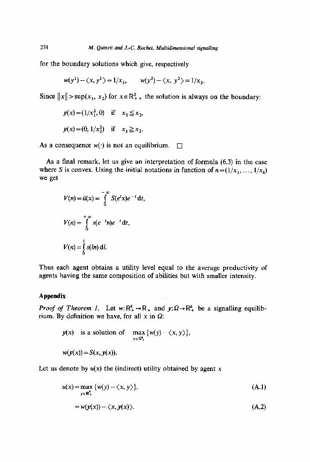
for the boundary solutions which give, respectively

W(Y’) - <x9 Y’> = l/Xl, NY”) - (x, Y2> = l/x,.

Since llxll >sup(x,, x2) for XE R2, + the solution is always on the boundary:

y(x) =( l/x:, 0) if x1 5 x2,

y(x) =(O, l/x$ if x1 2xX,.

As a consequence w(e) is not an equilibrium. 0

As a final remark, let us give an interpretation of formula (6.3) in the case where S is convex. Using the initial notations in function of n = (l/x,, . . . , l/x,J we get

V(n) = C(X) = ‘p” S(e’x)e-‘dt, 0

V(n) = +f s(e-‘n)e-‘dt, 0

V(n) = j s(h) dl. 0

Thus each agent obtains a utility level equal to the average productivity of agents having the same composition of abilities but with smaller intensity.

Appendix

Proof of Theorem 1. Let w: R$ -+R+ and y:sZ+[w: be a signalling equilibrium. By definition we have, for all x in Sz:

y(x) is a solution of rnnc {w(y) - (x, y)},

wti(x)) = S(x, Y(X)).

Let us denote by u(x) the (indirect) utility obtained by agent x

u(x) =max {W(Y) - <x, Y>>, FZ

(A.11

= wet(x)) - (x9 Y(X) >. (A-2)

M.

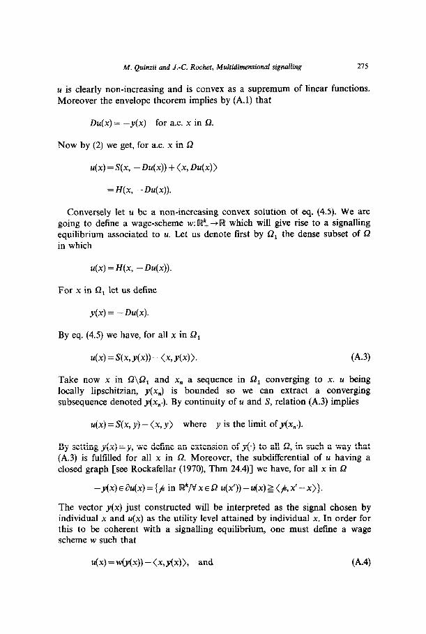
u is clearly non-increasing and is convex as a supremum of linear functions. Moreover the envelope theorem implies by (A.1) that

Da(x)= -Y(x) for a.e. x in 52.

Now by (2) we get, for a.e. x in Sz

u(x) = S(x, -h(x)) + (x, h(x))

= H(x, -h(x)).

Conversely let u be a non-increasing convex solution of eq. (4.5). We are going to define a wage-scheme w:aB: +[w which will give rise to a signalling equilibrium associated to a. Let us denote first by Sz, the dense subset of Sz in which

u(x) =H(x, -h(x)).

For x in Q, let us define

y(x) = -h(x).

By eq. (4.5) we have, for all x in Q2,

u(x) = w, Y(X)) - <x, Y(X)>. (A.3)

Take now x in 8\52, and x, a sequence in Q, converging to x. u being locally lipschitzian, Y(x,) is bounded so we can extract a converging subsequence denoted Y(x,.). By continuity of u and S, relation (A.3) implies

U(X) = S(x, y) - (x, y) where y is the limit of Y(x,,).

By setting Y(x) = y, we define an extension of y(a) to all 51, in such a way that (A.3) is fulfilled for all x in Sz. Moreover, the subdifferential of u having a closed graph [see Rockafellar (1970), Thm 24.4)] we have, for all x in B

-Y(X) E au(x) = (;kc in lRk/VxesL u(x))-u(x)~(#,x’--x>}.

The vector y(x) just constructed will be interpreted as the signal chosen by individual x and u(x) as the utility level attained by individual x. In order for this to be coherent with a signalling equilibrium, one must define a wage scheme w such that

44 =wti(x)) - <wM), and (A-4)


wdv(xN = 8% Y(X)). (A.5)

(A.4) and (A.5) are compatible because of eq. (A.3). By eq. (A.4) we must have

vx E Q w@(x)) = u(x) + (x&x)>. (-4.6)

Let us assume that y(xJ =y(xz) =y for some x1 #x2. Since y(v) is a selection of the subdifferential au(*) we have by definition

4x2) - 44 2 (Y, x1 -x2>, and

u(xl)-~tx2)~(Y,x2--xl).

Consequently

YW =Je2) =3 %) + <Xl~Y(Xl)> =4x2) + (X2,Y(X2)>.

Thus it is perfectly legitimate to define

w:[w: + R,

y + w(Y) = 44 + <x7 Y(X) > if 3 X/Y(X) = Y,

w(y) = 0 in the other case.

The only thing that remains to be proved is that, confronted with such a wage scheme, individual x will indeed choose signal y(x). Therefore we have to prove

VY E % 4Yb)) - <w44> 2 W(Y) - <xv Y>. (A.7)

If y # Range Q then w(y) - (x, y) 50 and (A.7) comes from the fact that

u(x) = d_Y(x)) - (x, Y(X)> 2 0.

If y=y(x’) for some x’ in Q then (A.7) is equivalent to

u(x) Zu(x’) + <x’-x&x’)>

which is a consequence of -y(x’) E&(X’). 0

Proof of Theorem 2. It is adapted from Lions (1983, pp. 26-28).


Step 1. u is non-increasing, with values in lR + .

Indeed: t(t) z x belongs to %Zs, so

U(x) 5 +Jrn e-‘H*(x, 0) dt =H*(x, 0), and 0

H*(x, 0) = sup H(x, y) < + co by assumption (A.3). YER5

Moreover H*(x, q) 2 H(x, 0) 2 0 for all (x, q) so that ii(x) 2 0. Finally since S is non-increasing in x by assumption (A.2), it is also the

case for H* and U. 0

Step 2. ii is convex.

It comes from assumption (A.4) which implies that H* is convex in (x,q)

since

so that H* is a supremum of convex functions of (x, 4). Now take E>O and

x=lx,+(l-2)x,, 1E]O, l[.

351 W1 such that u(q) 2 ‘jm e-‘H*(t,, g,) dt--E, 0

x2m2 such that U(xJ 2 ‘fm e-‘H*(c,, t,) dt--E, 0

Q being convex c =(ncl +(l -II)<,) belongs to %7x and

ii(x) 5 +jm e-‘H*((, 4) dt 0

which, by convexity of H* implies

Thus G(x) 5 Ati +( 1 -+i(x,) +E. Since this is true for all s>O, we have proved the convexity of U. 17


Step 3. ii is a subsolution to (4.5) i.e.,

U(x) 5 H(x, -E(x)) a.e. in 52. (A.8)

By the dynamic programming principle [see for instance Lions (1983, pp. 22- 23)] we have, for all t>O

IS(X) =r:f e-%(<(t)) +a e-“H*(t(s), t(s)) ds . = x

Thus for all u in IWk and t small enough t(s) =(x +su) belongs to B for all Olslt and --

u(x) s e-‘u(x + tu) + i e-W*(x + su, u) ds 0

which implies

O$i[e-‘u(x+tu)-u(x)]+fbe-“H*(x+su,u)ds.

Let t tend to 0. Since H*(., u) is measurable, the integral tends for a.e. x to H*(x, u); whenever U is differentiable in x, the first term converges to

Thus for all u in [Wk and a.e. x in 52:

4x) I {W(x), u> +H*(x, u)},

zi(x) s inf {(E(x), u) +H*(x, u)}. “ERk

By Fenchel’s duality theorem [see Rockafellar (1970)] the concavity of H(x, *) implies

inf {(Dzi(x), u) +H*(x, u)} =H(x, -E(x)) “ERk

and the proof of (A.8) is complete. 0


Step 4. denote by 4(v) the functional in formula (5.2):

(A.9)

We are going to prove that the intimum of 4 over ggx, which defines U(x), can be restricted to

G?;,={~&:,/vd=l,..., k VtzO -Ms[i(t)S5i(t)},

where M is the constant of assumption (A.2). By definition of H* we have

H*(x, 4 =T~u$ ((4 -x, Y> + Sk Y>>.

Thus H* has the following properties:

(i) if (q-x) $ rWk then H*(x, q) = + co

(ii) if qi< -M for some i then, by assumption (A.2)

VYE lR$ (aS/ayi)(X,y)+(qi-xi) <O and thus

H*(x, 4 = sup {S(x, Y) + (4 -x, Y>> Y& yi=o

so that H* is locally independent of qi.

Let us suppose that r in gx is such that, for some i in { 1,. . . , k} and to > 0

liCtO) ’ SittO).

Then, 5 being piecewise %‘l the same relation holds on some interval I:

4dt) > titt)v tgl.

It follows from property (i) that c$(() = + co. Similarly let us assume that for somej in {l,...,k) and t,>O we have


Let 5’ be a perturbation of 5 defined by

1

00) = x,

&t)=ti(t) for i#j,

4J(t)=SUp(-M, ~j(t)).

Then we clearly have, for all t>O:

c(t)?<(t) and thus l’(t) belongs to G!

~~~t)#~j(t)~ej(t)~-M=~~~t).

Since H* is non-increasing in x we have

Vt 20 H*(W), t(t)) S H*(W), &t>>.

It follows from (ii) and (A.lO) that

VtzO H*(<‘(t), &t))=H*(r’(t), t’(t)).

By a finite replication of the argument above, we have proved that

Step 5.

zi(x) = ,in,f 4(t). E x

U is a supersolution of (4.5), i.e.,

i(x) 1 H(x, -LX(x)) a.e. in 52.

Let us use again the dynamic programming principle, this’time on @,:

Vt>O “5(x)=(“of E x i

P’ti(~(t))+~e~“H*(~,~)ds

This implies, after dividing par (1 -em’)

1 o=sup-

tsax 1 -e-’ ii(x)-e-‘li(&t))-~e-sH*([, [)ds .

(A.lO)

q

(A.ll)

M. Quinzii and J.-C. Rochet, MultidimensionaL signalling 281

Whenever ii is differentiable at x, we have

lq(5(0) =+4 + <5(t)-% wd) + IIx-S(t)llEw

with lim,,, I = 0 since lim,,, t(t) =x. By an integration by parts we have

Therefore

U(X)-ii(t(t))e-‘=(l -e-‘)ii(x)- E(x), d &s)e-“ds >

+ LX(x), d (t(s) -x)e-“ds >

Combining with (A.ll), we get

&d C(W4 &s)> + H*(5, f)le-“ds

+ &b (DU(x), c(s)-x)e-“ds- e-’ 1 --em’

/lx-S@)lldf)}.

This implies

[@U(x), 4(s)> +H*(&), &4W”ds

(A.12)

But by definition of @‘, we have

Vi VsSO, -M 5 &(s) 5 &(s).


Thus by integrating we get, for all sst,

(i(s) - xi 2 - Mt and <i(s) $ x&.

Thus for all s $ t

In particular, when t+O:

115wxll 1 -e-’

is bounded.

Consequently,

sup tsBx

- e-’ 11x-i;(t)lle(t)]=v,(t)-0 when t-+0. l-e-’

(A.13)

Moreover

Fyt&[ (o4x),5(s)-x)e-“ds=v,(t)~O when t+O. (A.14)

Finally, H* being non-increasing in x, we have

vsst - H*(4W, &4> 5 - H*G=‘, &4>

since <E@~* <(s)sxxe”sxe’. Thus by (A.12), (A.13), (A.14) we get

OSti(x)- &a !i-$ [(hi(x), o) +iY*(xe’, u)]e-‘ds

+ Vl@) + v&)7

OSU(x) - inf [<Ofi( 0) +H*(xd, u)] + v,(t) +vJt). veR’

Using again Fenchel’s theorem and the concavity of H*(x, *) we get

05ii(x)-H(xe’, -LXi(x))+v,(t)+v,(t).

Since v1 and v2 tend to zero the continuity of H gives the announced property and the proof is complete. 0

M. Quinzii and J.-C. Rochet, Multidimensiona! signalling 283

Proof of Theorem 3. Let w(o) be a wage

c= {x @(x, Y,) $ W(Yo) + 4

which is convex by assumption (A.4). The Hahn-Banach Theorem implies

3pe Rk, QE R, sup <p, x) <a < inf <p, x). xeB XEC

Possibly redefining p, it is always possible to ensure that a < E. Consider now the new wage offer C

+W=wh)+a if Y=Y~+P,

G(y) = 0 if Y#Y,+P.

It is clear that all individuals in B choose this new offer and that any individual x doing the same must be such that

w(Y~) + a - (y. + P, x> 2 4Ax)) - tib), x> 2 4~~) - <yo, x>

which implies (p, x) 5 a and then x does not belong to C. Therefore

W, Y, + PI 2 W, yo) 2 4~~) + E > w(Y,) + a

which implies positive profit. 0

References

Akerlof, G.A., 1970, The market for ‘Lemons’: Qualitative uncertainty and the market mechan- ism, Quarterly Journal of Economics LXXXIV, 488-500.

Baron, D.P. and R.B. Myerson, 1982, Regulating a monopoly with unknown costs, Economet- rica 50, no. 4,91 l-930.

284 M. Quinzti and J.-C. Rochet, Multidimensional signalling

Cresta, J.P. and J.J. LaiTont, 1982, The value of statistical information in insurance contracts, GREMAQ DP 8212 (UniversitB de Toulouse, Toulouse).

Kohlleppel, L., 1983, Multidimensional market signalling, Universitlt Bonn, DP no. 125. Leland, H. and D.H. Pyle, 1977, Informational asymmetries, financial structure and financial

intermediation, Journal of Finance 32, 371-387. Lions, P.L., 1982, Generalized solutions of Hamilton-Jacobi equations (Pitman, London). Riley, J.G., 1975, Competitive signalling, Journal of Economic Theory 10, 174-186. Riley, J.G., 1979, Informational equilibrium, Econometrica 47, no. 2, 331-359. Rockafellar, R.T., 1970, Convex analysis (Princeton University Press, Princeton, NJ). Rothschild, M. and J.E. Stiglitz, 1976, Equilibrium in competitive insurance markets: An essay

on the economics of imperfect information, Quarterly Journal of Economics XC, 629649. Spence, A.M., 1973, Market signalling: Information transfer in hiring and related processes

(Harvard University Press, Cambridge, MA). Spence, A.M., 1974, Competitive and optimal responses to signals, Journal of Economic Theory

7, 296332. Williams, W.E., 1980, Partial differential equations (Clarendon Press, Oxford).

multidimensional signalling -...

Documents