Prof. John H. Munro munro5@chass.utoronto.caDepartment of Economics john.munro@utoronto.caUniversity of Toronto http://www.economics.utoronto.ca/munro5/

1 April 2009

ECONOMICS 303Y1

The Economic History of Modern Europe to1914

Prof. John Munro

Lecture Topic No. 29:

II. PROBLEMS AND GROWTH IN THE BRITISH ECONOMY, 1870 - 1914

A. Economic Trends, 1870 - 1914: the ‘Great Depression’ and the

‘Industrial Retardation’ Debates

B. British Financial Institutions and Capital Exports, to 1914

1

VII. PROBLEMS AND GROWTH IN THE BRITISH ECONOMY, 1870 - 1914

A. ECONOMIC TRENDS, 1870 - 1914: The DEBATES ON: ‘INDUSTRIAL

RETARDATION’ and ‘THE GREAT DEPRESSION’

1. The Current Debate about the British Economy, 1870 - 1914

There are really four inter-linked debates (and thus four different essay topics) on these issues,

about the British economy from 1870 to 1914:

a) The Debate about Industrial Retardation:

i) Did the British economy fail to cope adequately with the emergence of foreign industrial

competition after 1870,

# and consequently did it suffer some form of economic decline,

# if so, was that economic decline absolute or relative?

ii) Was such an economic decline, even if only relative, experienced in the form of a depression, or

economic stagnation, or in what is called ‘industrial retardation’?: i.e., a slowing down of the rate of

economic growth (as opposed to the absence of actual growth, or actual decline)?

iii) Did such ‘industrial retardation’ -- if it occurred -- govern the entire era 1870 to 1914, or just

part of this era?

iv) Did it indeed continue on after World War I, i.e., into the inter-war period, up to WWII?

b) The Debate about British Entrepreneurship:

i) Can be British businessmen, entrepreneurs, be held responsible for the supposed faults of the

British economy in this era?

ii) Can they be held accountable for failing to respond properly to foreign challenges?

iii) Was there a ‘Buddenbrooks’ syndrome?

(1) The renowned German author Thomas Mann (1875-1955) produced his earliest masterpiece

Buddenbrooks in 1901: situated in the German Baltic town of Lübeck

# a novel tracing the rise, decline, and fall of a Lübeck business family, over four generations,

# the last of which ruin the family fortunes established by the first and built up by the second.

(2) This theme of ‘rags to riches and back to rags’ can be seen historically, for example,

# in the 15th-century Florentine family of the Medici (over three generations)

# here in Toronto, in the Thomas Eaton family (do you remember Eaton’s?)

(3) But of course, if British business families rose, expanded, and then declined, they would not have

done so together, in the same periods: i.e., so that as one family’s fortunes declined another might be

rising in the same period.

iii) Or were the perceived faults those of industrial and financial structure that had evolved from

earlier in the nineteenth century? -- i.e., from the 1820s, without much relevance to foreign

competition.

iv) We have in fact already examined most of this issue, earlier: in the lectures on German

industrialization, especially lecture no. 24 (late February-early March)

c) The Problem of Capital Exports and post-1870 Capitalist Imperialism:

i) Did the British invest too heavily abroad at the expense of domestic investment? and

ii) Did the British thus rely too much on overseas investment incomes?

iii) Closely related to this topic is the still ongoing debate about Capitalist Imperialism, or the ‘New

Imperialism’ of the post 1870 era.

iv) the Marxist-Leninist theory of Imperialism: a summary

(1) that imperialism is ipso facto the export of capital abroad,

(2) but in particular to those areas offering higher investment returns than in the domestic economy,

(3) and thus British business necessarily had to export capital in order to avoid the fatal consequences of

the inevitable fall in the rate of interests and profits and rents at home, in the domestic economy:

(4) For this negative prediction was an axiom in 19th-century Classical economic theory, as well as a basic

principle of Marxism, that

# investment yields – in terms of profits, interest, and rent – have an inevitable historical tendency

to fall

# i.e., with increasing competition and growth of capital stock, etc.

(5) The Marxist belief was that, in response to this fall in investment yields, capitalists would necessarily

seek or strive to exploit their workers (in the Marxist view, the sole source of ‘surplus value’, and hence

of profits for the capitalists) far more intensively

(6) That increased exploitation, it was expected, would lead to industrial strife, strikes, and then

revolution.

d) The issue of the ‘Great Depression’ of 1873 - 1896: with several sub-issues

i) Did the international, European, or British economies suffer a ‘Great Depression’ after 1873:

specifically from 1873 to 1896?

ii) If not, why was there such a sharp and steep deflation in this period?

iii) What caused that deflation: real or monetary factors, or some combination of the two?

iv) Did the British and European economies then recover to experience a powerful pre-war

economic boom, from 1896 to 1914?

v) This was also a period of pronounced inflation: is the inflation itself evidence for an economic

boom?

vi) What were the causes of this inflation: again, monetary or real, or some combination of the two?

2. The Debate about the ‘Great Depression’ of 1873-96?

a) Was there such a ‘Great Depression’?

i) No, not for the entire period; and few if any historians, would now consider this entire era to have

been one of a ‘Great Depression’.

ii) Many, however, would contend that several commercial-industrial depressions or recessions did

occur during this era, along with alternating periods of boom or expansion; but that does not justify

using the term for the entire quarter-century.

b) Why then is the term ‘Great Depression’ so commonly used?

i) First, public perceptions:

(1) because British businessmen and government officials themselves in this era -- the 1870s and 1880s

# thought that they were experiencing depressions,

# ushered in by the international financial crisis of 1873.

(2) Indeed they believed so much in a depression that in 1884 the British government established a Royal

Commission to seek solutions for it.

ii) Second, monetary deflation and ‘money illusion’:

(1) because, as just noted, prices fell so sharply from 1873 to 1896 [see the graph]

(2) and along with prices also fell nominal interest rates and profits

(3) but not nominal or money wages, which generally continued to rise, if slowly: so that real wages rose

considerably.

iii) But third: were there any major economic costs arising from deflation? Yes, those that arose

from the stickiness of the factor costs of production.

(1) wages: as noted, money wages did not fall, while some in fact rose: historically, money wages have

always experienced or demonstrated downward stickiness (for reasons that I have sought to explain in a

journal article).1

(2) interest rates (price of borrowing capital):

1 John H. Munro, ‘Wage Stickiness, Monetary Changes, and Real Incomes in Late-Medieval England and the Low Countries, 1300 - 1500: Did Money Matter?’ Research in Economic History, 21 (2003), 185 - 297.

# most loan contracts specified a fixed rate of interest for the duration of the contract

# thus for long-term contracts, the annual interest payments would rise in real terms

# and the real cost of repaying the loan, with deflation (including presumably a fall in the price of

the product being manufactured and sold), would rise

(3) land rents: the same logic applies – and most rental contracts were long-term

(4) Did such a rise in the real factor costs of labour, capital, and land have any injurious effects on the

British economy during this period of deflation, from 1873 to 1896?

# so far no one has provided any such evidence

# but it may exist and be revealed by future research.

(5) Deflation as a stimulus to technological changes:

# Insofar as deflation did prove to be an economic problem, in raising factor costs as suggested,

above, then deflation may have been a positive spur to technological innovations to offset those

rising factors costs

# certainly there are abundant examples of many interrelated technological changes in British (and

other European) industries in this period

# And as noted, those technological innovations in turn are credited, to some extent, as real factors

that help to explain the deflation itself.

iv) Fourth, the problem of British Agriculture: because British grain farmers so clearly and definitely

suffered a very severe economic contraction (which is probably a better term than ‘depression’).

(1) particularly as and when the international transportation revolution finally brought home the bitter

fruits of Free Trade for the grain sector in particular, for agriculture in general, from the 1870s

(2) with sharply falling real prices, severe cut-backs in production, and that dramatic contraction in the

agricultural sector already demonstrated.

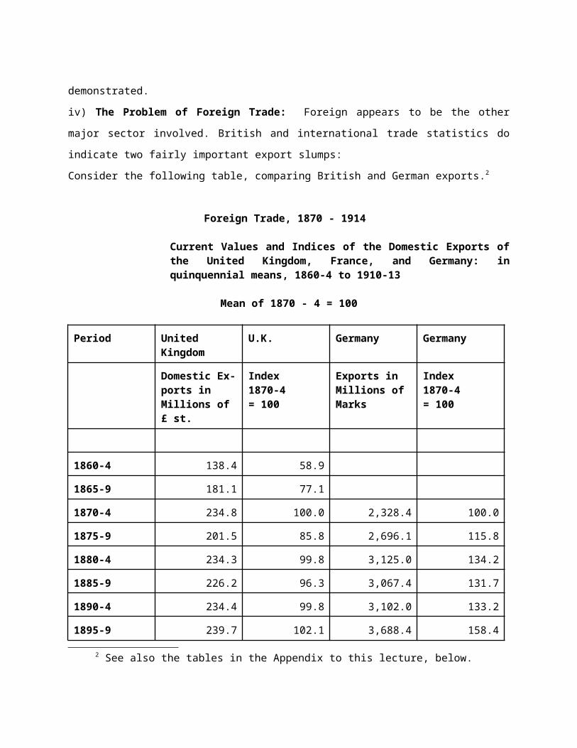
iv) The Problem of Foreign Trade: Foreign appears to be the other major sector involved. British and

international trade statistics do indicate two fairly important export slumps:

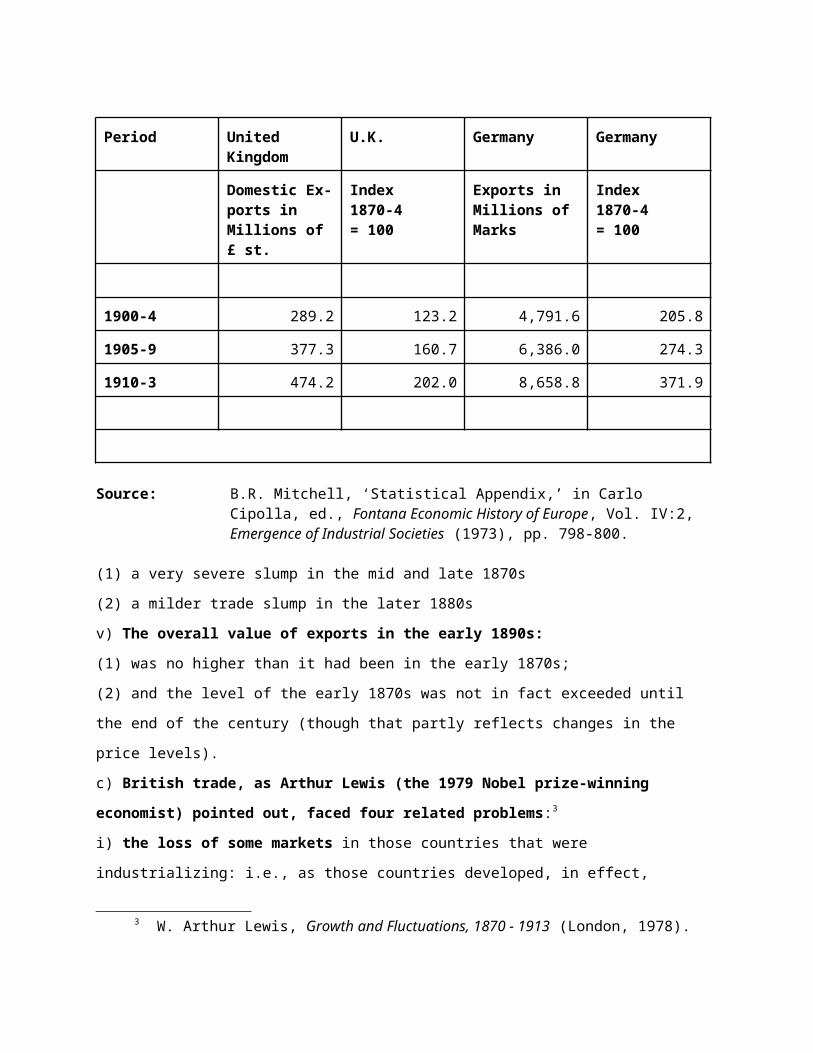
Consider the following table, comparing British and German exports.2

Foreign Trade, 1870 - 1914

Current Values and Indices of the Domestic Exports of the United Kingdom, France, and Germany: in quinquennial means, 1860-4 to 1910-13

Mean of 1870 - 4 = 100

2 See also the tables in the Appendix to this lecture, below.

Period United Kingdom U.K. Germany Germany

Domestic Ex-ports inMillions of £ st.

Index1870-4 = 100

Exports in Millions ofMarks

Index1870-4= 100

1860-4 138.4 58.9

1865-9 181.1 77.1

1870-4 234.8 100.0 2,328.4 100.0

1875-9 201.5 85.8 2,696.1 115.8

1880-4 234.3 99.8 3,125.0 134.2

1885-9 226.2 96.3 3,067.4 131.7

1890-4 234.4 99.8 3,102.0 133.2

1895-9 239.7 102.1 3,688.4 158.4

1900-4 289.2 123.2 4,791.6 205.8

1905-9 377.3 160.7 6,386.0 274.3

1910-3 474.2 202.0 8,658.8 371.9

Source: B.R. Mitchell, ‘Statistical Appendix,’ in Carlo Cipolla, ed., Fontana Economic History of Europe, Vol. IV:2, Emergence of Industrial Societies (1973), pp. 798-800.

(1) a very severe slump in the mid and late 1870s

(2) a milder trade slump in the later 1880s

v) The overall value of exports in the early 1890s:

(1) was no higher than it had been in the early 1870s;

(2) and the level of the early 1870s was not in fact exceeded until the end of the century (though that

partly reflects changes in the price levels).

c) British trade, as Arthur Lewis (the 1979 Nobel prize-winning economist) pointed out, faced four

related problems:3

i) the loss of some markets in those countries that were industrializing: i.e., as those countries developed,

in effect, import-substitution industries to produce goods formerly imported from Britain

ii) the loss of some markets in other or third countries that were being invaded by Britain's new

industrial rivals.

iii) the loss of relative access to many foreign markets: with the Return to Protectionism,

# i.e., with the restoration and rise of protective tariffs from the later 1870s.

# consider again the significance of Russia’s Mendeleyev Tariff of 1891: to block

entry of foreign goods and thus to force foreign producers to establish branch

plants within Russia

iv) the loss of some of Britain's own domestic or home market:

(1) Since Great Britain continued to practise complete Free Trade, with the Gold Standard, that market

was, and so was invaded by Britain's rivals.

(2) we have already seen the example of German steel products so strongly invading British domestic

markets.

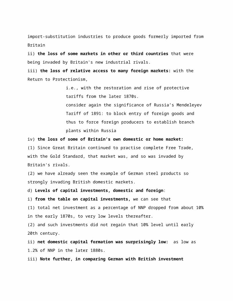
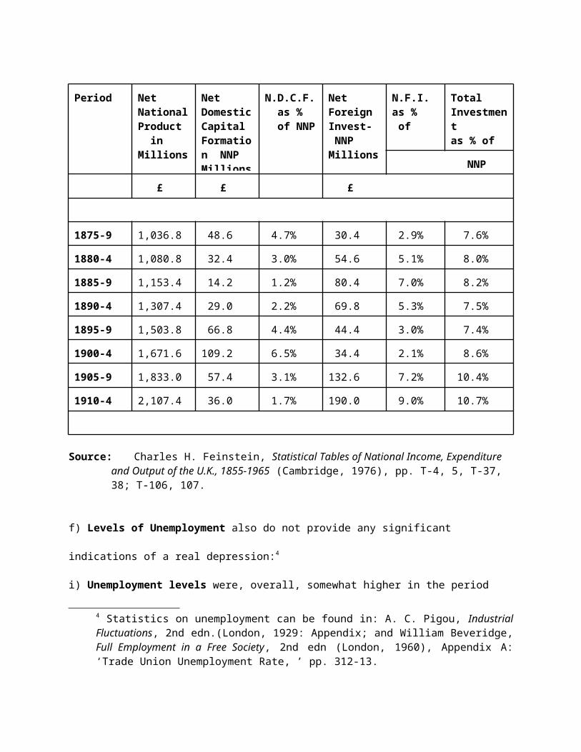
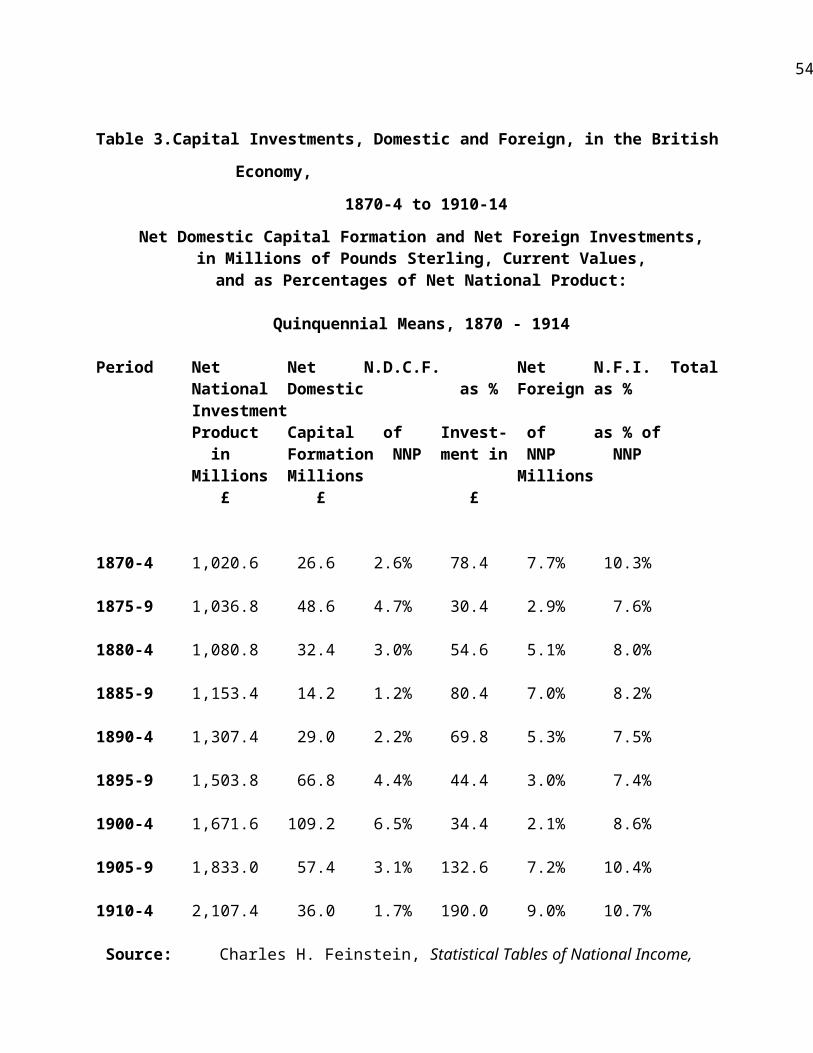
d) Levels of capital investments, domestic and foreign:

i) from the table on capital investments, we can see that

(1) total net investment as a percentage of NNP dropped from about 10% in the early 1870s, to very low

levels thereafter.

(2) and such investments did not regain that 10% level until early 20th century.

ii) net domestic capital formation was surprisingly low: as low as 1.2% of NNP in the later 1880s.

iii) Note further, in comparing German with British investment figures, how much lower the British

figures are.

Capital Formation Ratios in the UK and Germany, 1865 - 1904

in current nominal values and in constant 1913 values

3 W. Arthur Lewis, Growth and Fluctuations, 1870 - 1913 (London, 1978).

Years UK:

NDCF/

NDP

current

values

UK:

NDCF/

NDP

constant

values

UK:

NNCF/N

NP

current

values

UK:

NNCF/

NNP

constant

values

Germ-

any

NDCF/

NDP

current

Germ-

any

NNCF/

NNP

current

Germ-

any

NNCF/

NNP

constant

1860-

1870

7.2 8.6 10.0 11.5 8.5 9.7 10.6

1870-

1880

8.2 7.3 11.8 10.9 11.6 13.5 13.0

1880-

1890

6.4 3.4 10.9 8.1 11.2 14.0 14.5

1890-

1900

7.3 3.0 10.1 6.0 13.9 15.4 15.9

1900-

1910*

8.8 4.8 10.5 6.7 15.6 16.5 15.9

* For the UK: 1895-1904; for Germany: 1901-13

NDCF/NDP: Net Domestic Capital Formation as a Percentage of Net Domestic Product

NNCF/NNP: Net National Capital Formation (Total) as a Percentage of Net National Product

Source: Y. Goo Park, ‘Depression and Capital Formation: the United Kingdom and Germany, 1873 - 1896’, Journal of European Economic History, 26:3 (Winter 1997), p.514

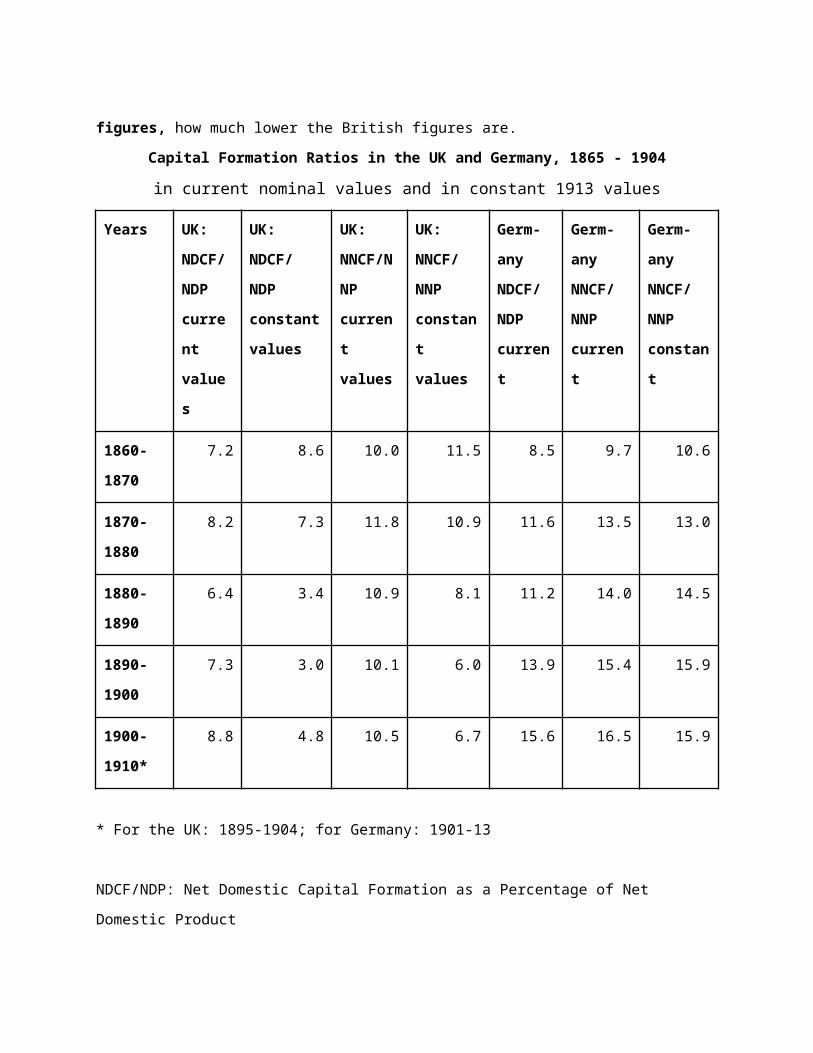
e) But there still remains no evidence for a genuine depression or even a secular economic decline

(apart from agriculture):

(1) note from the figures on Gross Domestic Product on the screen that GNP continued to rise over this

entire period,

(2) without any prolonged slumps that must characterize a depression.

(3) questions: what is depression, and also what is a recession?

Capital Investments, Domestic and Foreign, in the British Economy,

1870-4 to 1910-14

Net Domestic Capital Formation and Net Foreign Investments,in Millions of Pounds Sterling, Current Values,

and as Percentages of Net National Product:

Quinquennial Means, 1870 - 1914

Period

NetNationalProduct inMillions

NetDomesticCapitalFormation NNPMillions

N.D.C.F. as % of NNP

NetForeignInvest- NNPMillions

N.F.I.as % of

TotalInvestmentas % of

NNP

£ £ £

1870-4 1,020.6 26.6 2.6% 78.4 7.7% 10.3%

1875-9 1,036.8 48.6 4.7% 30.4 2.9% 7.6%

1880-4 1,080.8 32.4 3.0% 54.6 5.1% 8.0%

1885-9 1,153.4 14.2 1.2% 80.4 7.0% 8.2%

1890-4 1,307.4 29.0 2.2% 69.8 5.3% 7.5%

1895-9 1,503.8 66.8 4.4% 44.4 3.0% 7.4%

1900-4 1,671.6 109.2 6.5% 34.4 2.1% 8.6%

1905-9 1,833.0 57.4 3.1% 132.6 7.2% 10.4%

1910-4 2,107.4 36.0 1.7% 190.0 9.0% 10.7%

Source: Charles H. Feinstein, Statistical Tables of National Income, Expenditure and Output of the U.K., 1855-1965 (Cambridge, 1976), pp. T-4, 5, T-37, 38; T-106, 107.

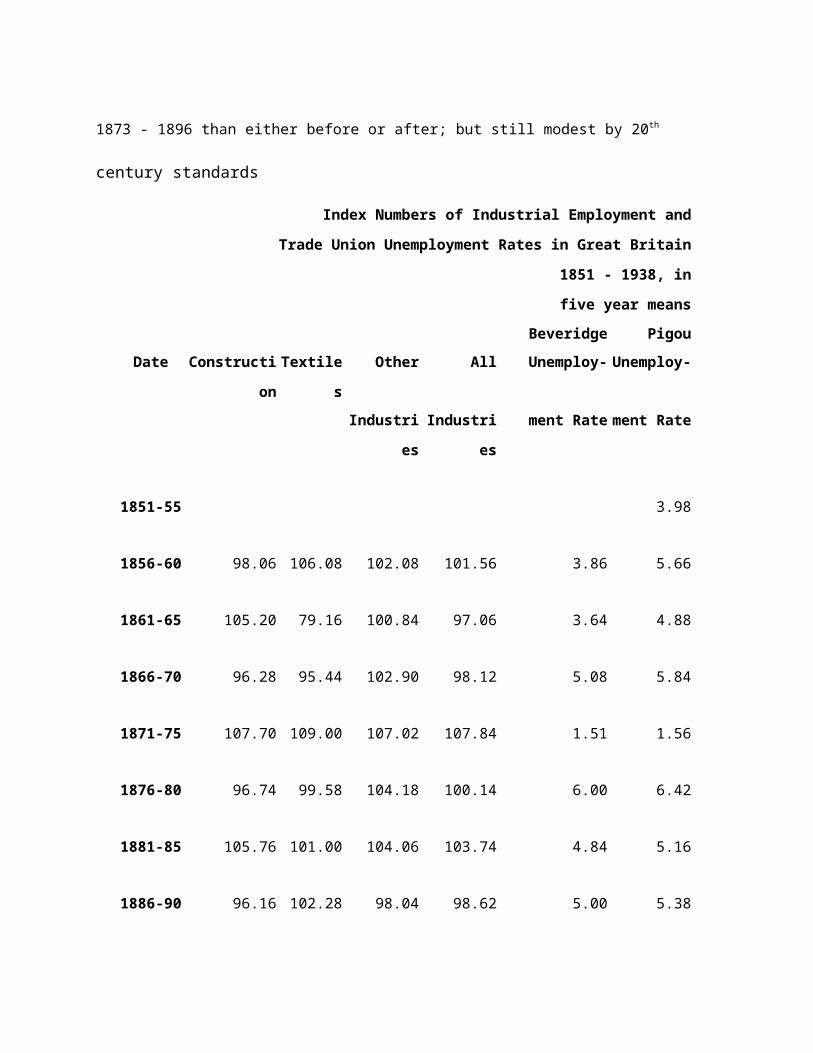
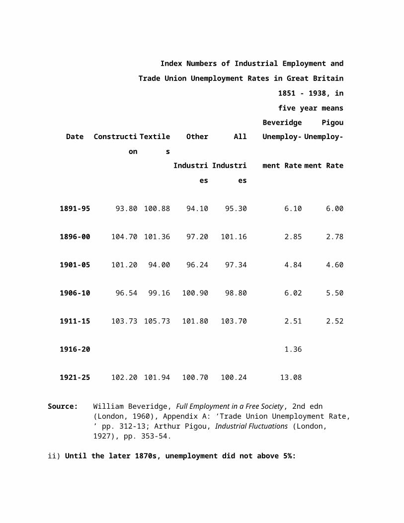
f) Levels of Unemployment also do not provide any significant indications of a real depression:4

4 Statistics on unemployment can be found in: A. C. Pigou, Industrial Fluctuations, 2nd edn.(London, 1929: Appendix; and William Beveridge, Full Employment in a Free Society, 2nd edn (London, 1960), Appendix A: ‘Trade Union Unemployment Rate, ’ pp. 312-13.

i) Unemployment levels were, overall, somewhat higher in the period 1873 - 1896 than either before or

after; but still modest by 20th century standards

Index Numbers of Industrial Employment and

Trade Union Unemployment Rates in Great Britain

1851 - 1938, in five year means

Beveridge Pigou

Date Construction Textiles Other All Unemploy- Unemploy-

Industries Industries ment Rate ment Rate

1851-55 3.98

1856-60 98.06 106.08 102.08 101.56 3.86 5.66

1861-65 105.20 79.16 100.84 97.06 3.64 4.88

1866-70 96.28 95.44 102.90 98.12 5.08 5.84

1871-75 107.70 109.00 107.02 107.84 1.51 1.56

1876-80 96.74 99.58 104.18 100.14 6.00 6.42

1881-85 105.76 101.00 104.06 103.74 4.84 5.16

1886-90 96.16 102.28 98.04 98.62 5.00 5.38

1891-95 93.80 100.88 94.10 95.30 6.10 6.00

1896-00 104.70 101.36 97.20 101.16 2.85 2.78

1901-05 101.20 94.00 96.24 97.34 4.84 4.60

1906-10 96.54 99.16 100.90 98.80 6.02 5.50

Index Numbers of Industrial Employment and

Trade Union Unemployment Rates in Great Britain

1851 - 1938, in five year means

Beveridge Pigou

Date Construction Textiles Other All Unemploy- Unemploy-

Industries Industries ment Rate ment Rate

1911-15 103.73 105.73 101.80 103.70 2.51 2.52

1916-20 1.36

1921-25 102.20 101.94 100.70 100.24 13.08

Source: William Beveridge, Full Employment in a Free Society, 2nd edn (London, 1960), Appendix A: ‘Trade Union Unemployment Rate, ’ pp. 312-13; Arthur Pigou, Industrial Fluctuations (London, 1927), pp. 353-54.

ii) Until the later 1870s, unemployment did not above 5%:

(1) for 1876-80, the mean was 6.00% (or 6.42%, according to Pigou’s earlier figures).

(2) the highest annual level was 10.70% in 1879

(3) The only other year of very high unemployment was 1886, with 9.55%

iii) In general, in the 1880s, unemployment averaged: 4.84% and 5.00% in each quinquennium

iv) Unemployment did not again reach the 6% level: until the end of this era, in 1891-95

v) and then fell sharply to just 2.85% in 1896-1900 (but rose to 6.02% in 1906-10).

vi) From 1911, and through that war-time decade: unemployment dropped sharply

vii) But rose sharply after World War I: with an astoundingly high mean of 13.08% in 1921-25.

3. The Course of Prices I: from 1873 to 1896:

a) The Period of the ‘Great Depression’, 1873 - 1896:

i) Deflation: This period, if not one of true depression, was nevertheless, as just noted, one of very severe

deflation, perhaps the severest deflation ever recorded (since the late 14th century), at least before that of

the 1930s.

ii) The Psychological Impact: as just emphasized, the steady fall in retail prices, interest rates, rents, and

in nominal profits, etc. was a major reason why contemporary businessmen thought that they were then

experiencing a depression.

iii) The real economic impact:

(1) If nominal money wages and nominal interest rates did not fall or adjust easily, to the overall decline

in the price level, then to repeat what was noted before:

(2) that provides obviously problems for many industrial and commercial entrepreneurs,

(3) or certainly those for whom wage and interest costs constitute a significant portion of their total costs,

for:

# interest rates on contracts obviously cannot be altered once a contract is issued

# historic problem of downward ‘wage-stickiness’: resistance of workers to wage cuts.

b) What was the cause of this deflation: monetary or real?

For this period (as indeed for many others, such as the 16th-century Price Revolution), there is an ongoing

debate in the journal literature between these two schools: monetary and real.

i) The ‘Real’ School: i.e., focusing on technological change, investments, populations, etc.: is led by

Rostow, Lewis, Landes;

ii) The monetary school: focusing on monetary factors (stocks and flows): is headed by Friedman,

Schwartz, and Bordo.

c) The Monetary School's arguments for deflation:

i) That almost all countries were now on the gold standard (Russia the last in 1894-97),

(1) with currency stocks determined by gold reserves;

(2) that the gold standard had the effect of isolating gold stocks and impeding world gold movements.

ii) That world gold supplies for monetary purposes were further dwindling,

(1) because there had been no new gold mining booms since those of the 1850s (California and

Australia); and,

(2) furthermore, because more gold was being consumed for industrial purposes.

(3) As you can see from the graph on the screen, and from Table 16, there was indeed a decline in world

gold mining outputs from the late 1860s, and a sharp decline in the early 1870s, followed by a general but

more gentle decline to the early 1890s

(4) note that the graph and table are expressed in decennial means, with the mid-decade point plotted on

the graph.

iii) That in general world money supplies failed to keep pace with the increasing volume of world

industrial production and trade:

iv) that in general, the monetary role is a passive one in deflation, as in the equation:5

M.V ≡ P.y [where y = NNI net national income = NNP net national product];

or M = k.P.y [in which k equals that proportion of NNI = P.y that the public chooses to hold in cash

balances, i.e., in high powered money that earns no investment income.

Thus, if y expands more than does M.V, then P must fall: If Δy > Δ (M.V) P ↓.⇒

v) Note that there is no clear evidence of any net contraction in national money stocks; no monetary

contraction as such.

(1) as for the gold question, as seen with Britain, France, and Russia, 19th century money supplies, with

the increasing role of bank credit, were no longer dependent upon gold stocks:

(2) there was no linear relationship between gold stocks and effective money supplies, as we just saw last

week, in examining Russian money and banking in the late 19th century.

v) Are the monetary arguments refuted by a fall in interest rates?

(1) Not necessarily, because it is the nominal rate of interest that fell, not real interest rates;

(2) and real interest rates in fact rose slightly with the much more pronounced deflation.

(3) Note that the real rate of interest = nominal rate minus the annual rate of inflation, or plus the annual

rate of deflation.

(4) This is the so-called Gibson Paradox, which was resolved in this fashion by Prof. Knick Harley.6

5 See my web document on the Quantity Theory of Money from Fisher to Friedman: http://www.economics.utoronto.ca/munro5/QUANTHR2.pdf

6 C. K. Harley, ‘Goschen's Conversion of the National Debt and the Yield on Consols’, Economic History Review, 2nd ser. 29 (1976), 101-06.

(5) In 1888, the British government converted its 3.0% Consols into 2.75% consols for this

reason.7

# in that the real return on 2.75% consols was equivalent to the earlier return on 3.0% consols;

#

7 Known as Goschen’s Conversion (after the Chancellor of the Exchequer), the act had another provision: that this rate of 2.75% would continue unchanged until 1902, then the rate would drop to 2.5%; and Consols still trade on the London Stock exchange today, at this same coupon of 2.5%, as noted last Fall in the lecture on the 18 th-century ‘Financial Revolution’.

i.e. to the real rate pertaining before 1870.

d) Arguments on the Real Side: appear, however, to be more solidly based.

i) Basic thesis: that the very sharp cost productions from an accelerating rate of technological change in

all sectors thus reduced prices throughout the economy:

(1) in industry, certainly; in transportation; in agriculture;

(2) and with sharp reductions in transaction costs from greater efficiencies in the commercial and

financial sectors.

ii) We have already seen many impressive examples:

(1) the tremendous growth in world agricultural production, with many new low cost areas servicing

world food markets, with cheap transport;

(2) and thus: the fruition of the transportation revolution in railroads and steam shipping, world wide,

leading to a dramatic fall in shipping rates;

(3) the revolution in steel, for which we recently noted that steel costs and prices fell over 80% from the

1860s to the 1890s.

(4) the Second Industrial Revolution in mechanical power: with the new electrical, chemical industries,

and internal combustion (automotive) industries;

(5) plus quite dramatic changes in the consumer goods industries to be seen shortly and in the distribution

trades, which all reduced consumer prices considerably.

iii) Note that dozens or hundreds of interrelated minor technical changes had collectively a far

greater impact than isolated dramatic changes.

iv) Added to this is the tremendous expansion in the world production and trade of a tremendous

range of agricultural and industrial commodities, as both continental Europe and the Americas began

industrializing.

v) Nevertheless this real side does not negate the validity of the previously mentioned monetary

side: we still come to the same conclusion that, in terms of modern income version of the quantity theory,

y expanded much more than M.V combined, so that prices had to fall.

e) Johnson’s ‘Monetary Approach to the Balance of Payments’:

i) It is also possible to argue that world gold stocks did determine world price levels; but obviously

also in relation to the world production and distribution of goods and services.

ii) In turn world prices are transmitted to each country via international commodity and capital

flows, especially with fixed exchange rates under the international gold standard.

iii) Those prices at the national level then help determine the quantity of money, via the banking

system, required for all economic transactions.8

f) For Great Britain in particular: keep in mind two very important economic factors that meant an

almost automatic transmission of changes in foreign or world prices to the British economy (more so than

for other European countries):

i) Free Trade: with no barriers to entry of foreign goods.

ii) The Gold Standard: which meant fixed exchange rates, with each country's currency pegged to fixed

units of gold and freely convertible into gold and into each other.

iii) Both meant: the free flow of capital as well as of goods.

4. The Course of Prices II: 1896 - 1914 :

How then do we explain the reversal of price trends, and the obviously inflationary upsurge in prices

world wide after 1896, up to and including World War I?

a) The basic Real Theory does not seem to fit so well here:

i) Can we say that technological changes were less fruitful or less cost-cutting after 1890s than

before?

(1) On the face of it, that seems most unlikely and unreasonable when we remember in particular

# the great productivity gains achieved in German industry from the 1890s,

# especially in the steel, chemical, and electrical industries.

# and in world-wide transportation costs (though most achieved by the 1890s).

(2) Certainly in the first two, the greatest gains came after 1890.

ii) But this issue does depend on the country

(1) and for Great Britain we shall shortly see some considerable evidence (from Feinstein's recent

publications) that industrial growth rates were indeed falling from the 1890s:

(2) growth rates were much lower from 1895 to 1914 than they had been before then.

iii) For world agricultural production, and possibly the production of raw materials in general, W.A.

Lewis does argue some such theory on falling productivity: rising marginal costs of grain production and

in world distribution:9

We have seen that US wheat exports were declining absolutely. To make up the deficit, the world 8 See: Harry Johnson, ‘Towards a General Theory of the Balance of Payments,’ in his International Trade and Economic Growth (London, 1958), pp. 153-68; Harry Johnson, ‘The Monetary Approach to Balance of Payments Theory,’ in his Further Essays in Monetary Theory (London, 1972); and Jacob Frenkel and Harry Johnson, ‘The Monetary Approach to the Balance of Payments: Essential Concepts and Historical Origins,’ in J.A. Frenkel and H.G. Johnson, The Monetary Approach to the Balance of Payments (Toronto, 1976), pp. 21-45.9 W. A. Lewis, Growth and Fluctuations, 1870-1913 (London, 1978).

had to turn to expansion of wheat production in Canada, Argentina, Australia, Russia, and Central Europe. Costs were higher in those countries because they were less mechanized; moreover transportation costs to Europe were higher from Argentina or Australia than from the USA. So even if volume sold had been the same, the price would have been higher. In sum, we find as follows: First the original cause of the Kondratiev swing lies in changes in the rate of flow of agricultural output. Secondly, these changes had cumulative effects on the price level...

[But unfortunately Lewis fails to show precisely and mathematically how ‘these changes had

cumulative effects on the price level...’]

b) A Keynesian variant: following in particular W.W. Rostow, we could attribute the price recovery and

subsequent inflation to the very expansionary effects of three related factors: in terms of the formula for

national income determination (and the inflationary gap):

Y = C + I + G + (X - M)

i) substantially higher levels of capital investments, in particular foreign investments, with much

longer gestation periods: i.e., to reach fruition in producing consumer goods to sop up consumer

demand.

ii) A new export boom, partly financed by those foreign investments, doubling exports between 1895

and 1914.

iii) thirdly, unproductive and therefore clearly inflationary investments in military production:

from the Boer War of the 1890s to World War I.

c) The Monetary Explanations: also bear some weight here.

i) The major and most dramatic event was gold mining:

(1) the two gold mining booms of the mid 1890s in South Africa and the Yukon.

(2) As the graph (and table on which it is based) clearly demonstrate: there is a truly dramatic increase in

world gold-mining outputs, veritably an explosive increase

(3) In decennial means, total outputs rise from an annual mean of 135.0 metric tonnes in the 1880s:

# to one of 255.6 metric tonnes in the 1890s,

# then more than doubling to a mean of 513.9 metric tonnes in the early 20th century (up to WWI).

ii) Great expansion in world gold movements and bank gold reserves:

(1) evidently led to a considerable expansion in currencies and bank lending, probably exceeding the

growth in world production and trade.

(2) It must be stressed once more, however, that there is no linear relationship between growth in gold

stocks and in the expansion of the money supply, whether reckoned as M1 or M2.

iii) Note that Rostow considers gold mining to be inflationary itself: the capital investment produces

employment and investment incomes, but without any new consumer goods to match.

5. Industrial Trends and the ‘Retardation’ Question

a) The price trends can be misleading:

i) The prolonged deflation of 1873-1896 does not mean an overall depression: or even stagnation for

this period;

ii) nor does the prolonged inflation of 1896-1914 mean an overall economic boom with stronger

growth for that period; to the contrary.

iii) As the national income tables on the screen show:

(1) there is general economic growth over the entire period, from the 1870s to 1914 (WWI),

(2) though incontestably there were years of economic slump or slowdown.

b) But what about rates of economic and particularly industrial growth?

i) do they show any slackening or slowing down, i.e., retardation?

ii) How do British growth rates in this period 1870 - 1914 compare with prior and succeeding periods;

iii) How do they compare with those for other nations?

6. The Statistical Evidence :

On this question, as tables show, the statistical evidence is mixed:

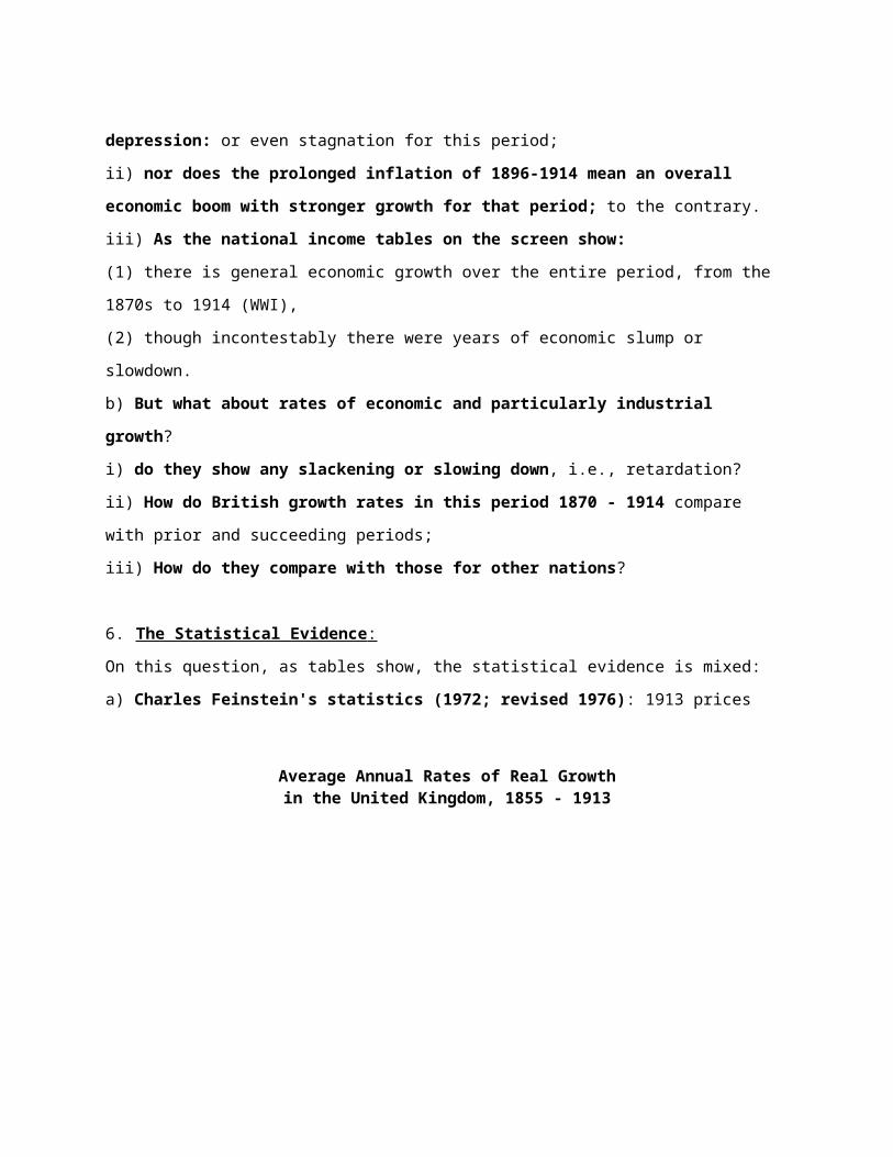
a) Charles Feinstein's statistics (1972; revised 1976): 1913 prices

Average Annual Rates of Real Growthin the United Kingdom, 1855 - 1913

Period Years Total Real Gross Domestic Product

(No.) Industrial at Constant Factor Prices

Output (at (from output data)

constant price)

1855-1913 59 2.29% 1.87%

Period Years Total Real Gross Domestic Product

(No.) Industrial at Constant Factor Prices

Output (at (from output data)

constant price)

1870-1913 44 2.09% 1.82%

...............................

1855-69 15 2.08% 1.63%

1870-84 15 2.04% 1.71%

1885-99 15 2.91% 2.14%

1900-13 14 1.60% 1.64%

Source: Charles Feinstein, Statistical Tables of National Income, Expenditure, and Output of the United Kingdom, 1855 - 1965 (Cambridge, 1976).

Notes:

i) These growth rate statistics do show that the overall rate of economic growth for the entire period

1870 - 1914 was slightly less than for the longer comparison period 1855 - 1913, and thus for the prior

period of 1855 - 70.

ii) But of the sub-periods given, note that the period 1885-99 showed a significant increase in both

industrial output and in GNP: and note further that two-thirds of this period are supposedly years of the

‘Great Depression’ (1873-96).

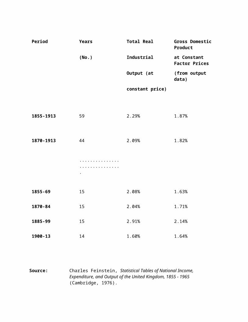
b) A.R. Lewis's Statistics:

i) A somewhat different picture, however, is provided by W. Arthur Lewis's statistics of 1978: from

his Growth and Fluctuations, 1870 - 1913 (London, 1978):

Average Annual Growth Rates inthe United Kingdom, 1853 - 1913

Period Number of Manufacturing Gross Domestic Productof Growth Rates Years and Mining at 1907 Prices

1853-1873 20 2.7% 1.95%

1873-1883 10 2.2% 1.90%

1883-1899 16 2.1% 1.85%

1899-1913 14 2.0% 1.70%

ii) Notes:

(1) Lewis uses slightly different time periods from those of Feinstein, with different estimates of GDP (at

1907 prices), and a different index of manufacturing production, excluding construction (housing,

buildings).

(2) His figures (with higher rates generally) show a consistent and overall pattern of decline in growth

rates from 1873 to 1914, in both Manufacturing and Mining and also in Gross Domestic Product.

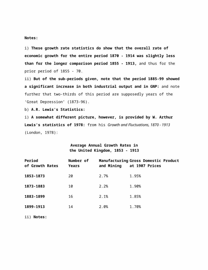
c) Feinstein, subsequently (in August 1990), retaliated with a new set of statistics:

i) This time the measurement is Real Gross Domestic Product per Worker: measured three different

ways:

ii) measurements: by income data, by expenditure data, and by output data (none of them agreeing with

each other, though showing somewhat similar overall trends):

Real Gross Domestic Product per Worker, 1856 - 1913Average Annual Percentage Rates of Growth

Period Income Expenditure Output

1856 - 73 1.32 1.38 1.12

1873 - 82 0.90 1.03 1.20

1882 - 99 1.49 1.27 0.85

1899 - 1913 0.09 0.33 0.72

.....................................

1856 - 1882 1.18 1.26 1.15

1882 - 1913 0.86 0.84 0.79

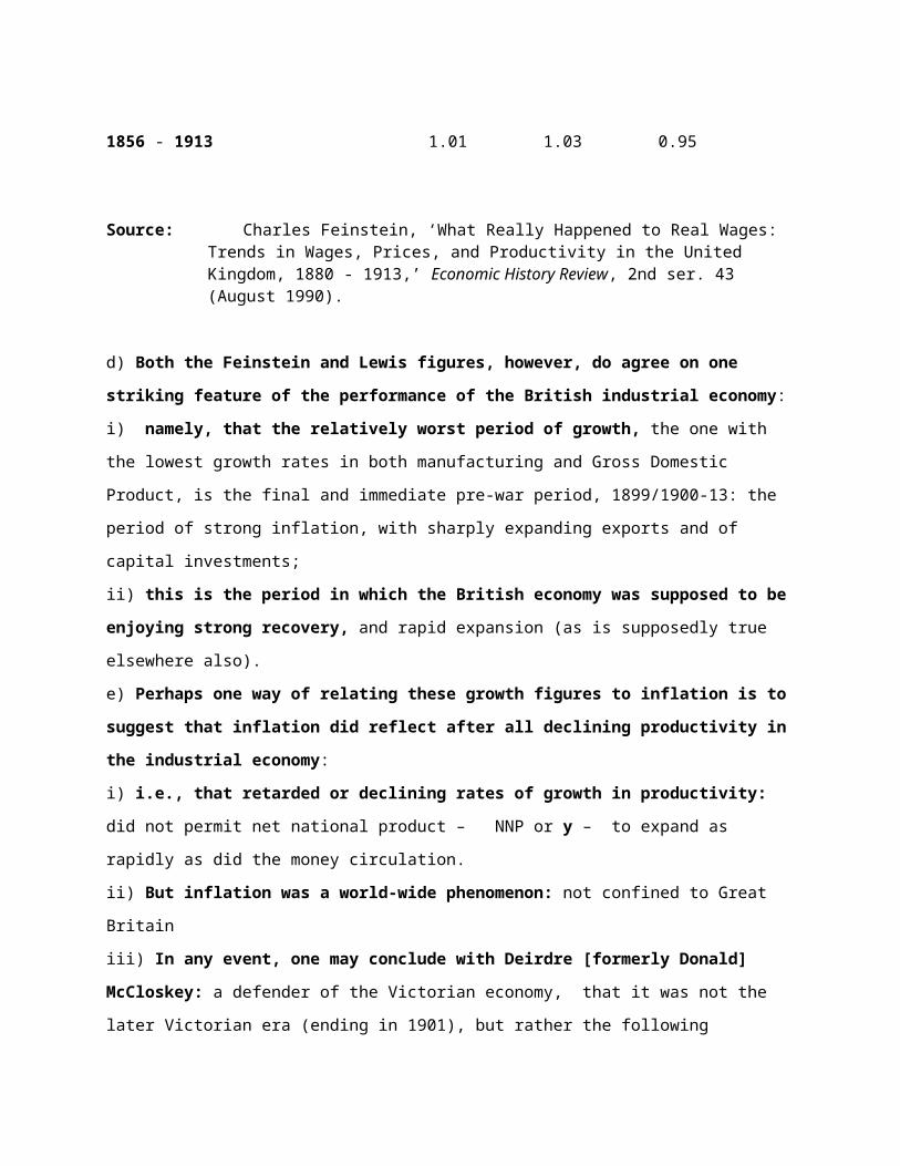
1856 - 1913 1.01 1.03 0.95

Source: Charles Feinstein, ‘What Really Happened to Real Wages: Trends in Wages, Prices, and Productivity in the United Kingdom, 1880 - 1913,’ Economic History Review, 2nd ser. 43 (August 1990).

d) Both the Feinstein and Lewis figures, however, do agree on one striking feature of the

performance of the British industrial economy:

i) namely, that the relatively worst period of growth, the one with the lowest growth rates in both

manufacturing and Gross Domestic Product, is the final and immediate pre-war period, 1899/1900-13: the

period of strong inflation, with sharply expanding exports and of capital investments;

ii) this is the period in which the British economy was supposed to be enjoying strong recovery, and

rapid expansion (as is supposedly true elsewhere also).

e) Perhaps one way of relating these growth figures to inflation is to suggest that inflation did

reflect after all declining productivity in the industrial economy:

i) i.e., that retarded or declining rates of growth in productivity: did not permit net national product –

NNP or y – to expand as rapidly as did the money circulation.

ii) But inflation was a world-wide phenomenon: not confined to Great Britain

iii) In any event, one may conclude with Deirdre [formerly Donald] McCloskey: a defender of the

Victorian economy, that it was not the later Victorian era (ending in 1901), but rather the following

Edwardian era that is the true period of relative retardation.

iv) Lewis, however, would still insist, however, that the period overall from 1870 to 1914 was one of

continuing decline in economic growth rates;

v) But I will leave it do you to decide amongst the Lewis and Feinstein statistical data.

f) Comparisons of British Industrial Growth with the French, German, and American from 1860 to

1914:

i) Finally, we cannot escape the undeniable fact that Britain's industrial growth rates in this period

overall are considerably less than those for the United States and Germany:

(1) less than half Germany’s and only third of the American growth rates.

(2) And indeed no better than France's growth rate, in a period when France was accused of suffering

economic stagnation.

ii) As for Germany and the U.S.: we have already seen how they overtook Great Britain rapidly in many

key industrial sectors: in steel-making (in aggregate terms, but not in all types of steel-making), in the

new chemical and electrical industries especially.

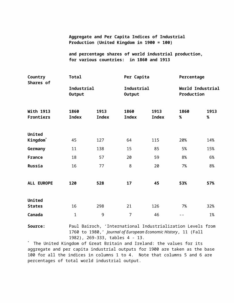
iii) If we can believe the statistics of Paul Bairoch on the screen: from The Journal of European

Economic History, 1982: by 1913, the United States was accounting for more than twice as much

industrial production as the British (32% of world output vs. 14%); and Germany for slightly more (15%).

Aggregate and Per Capita Indices of IndustrialProduction (United Kingdom in 1900 = 100)

and percentage shares of world industrial production, for various countries: in 1860 and 1913

Country Total Per Capita Percentage Shares ofIndustrial Industrial World IndustrialOutput Output Production

With 1913 1860 1913 1860 1913 1860 1913Frontiers Index Index Index Index % %

UnitedKingdom* 45 127 64 115 20% 14%

Germany 11 138 15 85 5% 15%

France 18 57 20 59 8% 6%

Russia 16 77 8 20 7% 8%

ALL EUROPE 120 528 17 45 53% 57%

UnitedStates 16 298 21 126 7% 32%

Canada 1 9 7 46 -- 1%

Source: Paul Bairoch, ‘International Industrialization Levels from 1760 to 1980,’ Journal of European Economic History, 11 (Fall 1982), 269-333, tables 4 - 13.

* The United Kingdom of Great Britain and Ireland: the values for its aggregate and per capita industrial outputs for 1900 are taken as the base 100 for all the indices in columns 1 to 4. Note that columns 5 and 6 are percentages of total world industrial output.

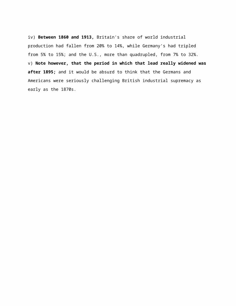
iv) Between 1860 and 1913, Britain's share of world industrial production had fallen from 20% to 14%,

while Germany's had tripled from 5% to 15%; and the U.S., more than quadrupled, from 7% to 32%.

v) Note however, that the period in which that lead really widened was after 1895; and it would be

absurd to think that the Germans and Americans were seriously challenging British industrial supremacy

as early as the 1870s.

B. British Banking: the Response to Continental Investment Banking

1. Features and Faults of the British Banking System, 1870 - 1914

a) If inadequate domestic investments, i.e., capital formation, are deemed to be a fault of the post-

1870 British economy, did the fault lie with the British banking system?

i) Was it an institutional fault?

(1) i.e., the failure to adopt investment banking according to the continental model really established by

the French bank Crédit Mobilier in 1853?

(2) The standard view, of course, is:

# that the British did not engage in such investment banking,

# if only because it was not really required, with Britain’s more highly developed capital

markets and alternative financial institutions to raise and invest such capitals.

ii) Consider Gerschenkron's following comment on European banking:10

The difference between the banks of the crédit-mobilier type and commercial banks in the advanced country of the time (England) was absolute. Between the English bank essentially designed to serve as a source of short-term capital and a bank designed to finance the long-run investment needs of the economy there was a complete gulf. The German banks, which may be taken as a paragon of the type of the universal bank, successfully combined the basic idea of the crédit mobilier with the short-term activities of commercial banks [and thus are now commonly known as Universal Banks]

b) But was there no positive response from this older British banking system, such as the one found

in France?

i) In discussing the conflict between the New and Old Banks, between Crédit Mobilier and the

Rothschilds (the Paris Branch), Gerschenkron also comments, as follows:

...what is so seldom realized is that in the course of this conflict the ‘new wealth’ succeeded in forcing the old wealth to adopt the policies of its opponents. The limitation of old wealth in banking policies to flotations of government loans and foreign exchange transactions could not be maintained in the face of the new competition. When the Rothschilds prevented the Pereires [Brothers] from establishing the Austrian Credit-Anstalt [bank], they succeeded only because they became willing to

10Alexander Gerschenkron, Economic Backwardness in Historical Experience: A Book of Essays (New York, 1962; reissued in paperback in 1965): in particular ‘Social Attitudes, Entrepreneurship, and Economic Development,’ pp. 52-71.

establish the bank themselves and to conduct it not as an old-fashioned banking enterprise but as a crédit mobilier, that is, as a bank devoted to railroadization and industrialization of the economy.

ii) So was there any such similar response in Britain from the 1850s?

2. British Forays into Investment Banking, 1860 - 1914

a) Baring Bros of London (a family-owned merchant bank, of Dutch origin) and Glyn, Mills & Co.

(joint-stock bank) worked together in new forms of investment banking, to engage in:

i) railway financing, at home and abroad, especially in North America; and

ii) in the financing of some foreign banks: especially

# the Ottoman Bank (1856)

# the Bank of London and South America (1863), and

# the Anglo-Austrian Bank (1864).

iii) and also in overseas lending: especially in foreign state loans.

iv) Amongst joint-stock banks:

(1) two such banks – Glyn, Mills and Co. and the Union Bank of London – seem to have been the very

few exceptions to engage in such forms of direct investment banking

(2) especially in North American railway financing.

b) Such financing was in the form of both long-term loans and in equity: i.e., in underwriting stock

issues, as the table on the screen indicates (with Baring Bros. as the leader).

c) Investment and commercial roles of London merchant banks:

i) London merchant banks were just that: commercial businesses whose primary role was in

international trade, and whose banking activities were related to financing that trade

ii) Baring Brothers were very actively engaged in overseas trade, certainly until the 1870s, when they

shifted more and more to finance.

iii) In the 1880s, Barings, Hambros, Gibbs and some other merchant banking houses

(1) did undertake and underwrite share issues in brewery houses,

(2) which ‘are sometimes cited as an exception to the inhibitions of the system’;

(3) but in any event this new interest evaporated quickly in 1890 [with the Baring crisis over Argentinian

loans].’

iv) Consider Stanley Chapman's quote on general bank avoidance of stock underwriting: ‘Most of

the merchant bankers, like the Rothschilds, “just took a bite or two at the cherry and retired, finding the

morsel not so tasty as they expected”.’11

v) Basic Problems: industrial scale and the costs of underwriting:

# Chapman points out that the costs involved -- in terms of bank commission (up to 5%),

underwriting commission, brokerage fees, advertising, legal fees -- made underwriting

too expensive for most merchant banks, so that:

# ‘even as late as the 1930s, any issue below £200,000 or £250,000 was reckoned to be

uneconomic’.

# ‘Before the First World War, companies of this size [i.e., with that amount of

capitalization] were still exceptional.’

vi) Stockbrokers and the financial press: greatly influenced investing public and did not direct such investors to merchant banks.

2.Chapman's Conclusions on British Merchant Banking in the later 19 th Century :

a) role of English merchant-banking in 19th century marginal and unimportant:

i) Quotation: ‘London merchant banks did not become seriously interested in industrial issues until

their traditional business fell away to nothing and the average size of companies rose to meet their ceiling.

Case studies show that, even then, there were major problems in directing thinking towards new

opportunities’.

ii) Thus there was not really a substantial shift towards genuine investment banking in Britain until

after World War II.

b) retained emphasis on acceptance banking over merchant banking:

‘The evidence of this book serves to emphasise that, with very few exceptions, the merchant banks were

much more commonly interested in acceptances [bills of exchange] than [in stock] issues...’

c) The example of N[athan] .M. Rothschilds and Sons (founded in London in 1798)

i) despite the engagement of the continental Rothschilds in investment banking, the London

Rothschild bank generally eschewed and avoided any forms of industrial investment banking, contenting

themselves to their traditional roles in ‘bonds, bills, and bullion.’

ii) N.M. Rothschild did, however, engage in considerable underwriting of foreign state loans and bonds,

often in financial syndicates; and had done so since the Napoleonic Wars.

iii) Many of these state loans, by Rothschilds, Baring Bros, and other merchant banking houses, were

in fact used to finance railways in these countries.

11 Stanley Chapman, The Rise of Merchant Banking (London, 1984), pp. 120-22.

iv) in the volume of loans, national and international, Rothschilds was always well ahead of Baring

Brothers.

d) Final Observations of Stanley Chapman on British banking and industrial financing:

i) ‘Most economic historians have agreed that the London capital market was biased towards

overseas investment, neglecting the opportunities of domestic industry, and Professor Saville and others

have seen clear evidence of lack of entrepreneurial spirit in the situation.’

ii) Chapman's explanation: is based upon

(1) the family-nature and family-capital control of most merchant banks,

(2) their diverse international origins in many cases (seeking freedom of trade and finance in London),

(3) and their extensive international mercantile connections.

iii) Such comments: are thus very close to those so commonly made against French banking!

e) International Role of British banking:

i) Chapman: ‘In 1914 British accepting houses still dominated the finance of world trade. In 1914 --

indeed until the crisis of 1931 -- international trade was still largely conducted in sterling bills on

London.’ (Chapman, p. 124).

ii) British dominance can be explained not only by the role of British shipping, commerce, and

banking.

iii) but also by the role of a large number of international banks, attracted by London's international

status, which established branches in London, and which thereby developed close relationships with each

other.

iv) Thus a conclusion may still remain that the British banking system diverted too much of

available investments sources, capital, abroad rather than at home; but that conclusion still needs to

be verified (i.e., in terms of comparisons with potential domestic capital investments, including domestic

demand for such investments and the willingness of British firms to depend upon German-style

investment banks).

4. Summary of Reasons why British investment banking was so limited in scale: Some Recent

Views

a) traditional British banks, both family firms and joint-stock company banks, continued the

established tradition of focusing mainly on commercial deposit banking with discounting and short-term

lending.

i) Recently several articles have appeared that reinforce, with both statistics and complicated

econometric analyses, these same conclusions:

ii) Two of these are the by the British team: of Mae Baker and Michael Collins:12

b) Baker and Collins on British Investment Banking:

i) They contend that British bank conservatism, and an orientation to short term lending, became

even more, all the more pronounced after two major banking crises from the 1870s:

(1) 1878: the collapse of the City of Glasgow Bank, a joint-stock bank with 133 branches,

# which, however, despite the 1862 legislation, had not offered its shareholders limited

liability,

# believing that creditors would have more faith in the bank if they believed that

shareholders would be fully responsible for all deposits, loans, and other legal

obligations.

(2) 1890: the Baring Crisis, in which the collapse of this very major merchant-investment bank was

avoided only because the Bank of England did step in to act as a Lender of Last Resort, while organizing

a financial consortium to guarantee the loans made by Baring Brothers.

ii) Both crises were due to unwise lending with insufficient liquid assets:

(1) City of Glasgow Bank (1878):

# far too much of its loans were concentrated with too few, and unreliable borrowers,

# a problem complicated by management fraud, and obviously not resolved by imposing

unlimited liability upon the shareholders.

(2) Baring Crisis of 1890:

# 75% of Baring’s assets were in loans to the governments of Argentina and Uruguay, for

whose economies boom turned to bust in 1890,

# preventing Argentina in particular from paying interest on its outstanding loans.

# History sometimes repeats itself: consider Argentina’ recent financial disasters, in and

after 2002

iii) They argue that these, by far the two worst financial crises of the 19th century, caused almost all

British banks to become far more conservative in their lending and to increase their liquidity

iv) Two-fold response: which is born out by their econometric analyses:

(1) to readjust the structure of their finances and bank assets in particular: to shift their assets away from

industrial private-sector credits into proportionately larger cash reserves and more liquid assets in the

12 Mae Baker and Michael Collins, ‘English Industrial Distress Before 1914 and the Response of English Banks’, European Review of Economic History, 3:1 (April 1999), 1-24; Mae Baker and Michael Collins, ‘Financial Crises and Structural Change in English Commercial Bank Assets, 1860 - 1913’, Explorations in Economic History, 26:4 (October 1999), 428-44.

form of short-term government bonds, etc.

(2) Thus in general a shift from whatever longer-term industrial finance they had engaged in to much

more short-term, fully collateralized lending.

(3) And from proportionately fewer investments or loans in the private industrial sector to thus

proportionately more in the public sector, i.e., municipal and state bonds.

English Commercial Banking Asset Ratios (percentages)

Years Private Sector Loans

Advances Bills Investments Cash

1860 69.4 46.7 30.7 16.2 13.1

1870 75.9 49.0 33.6 13.3 13.8

1880 65.1 47.6 20.0 17.7 19.2

1890 62.6 50.1 15.7 18.5 17.8

1900 57.0 50.6 11.1 22.8 18.7

1910 54.0 48.0 10.2 22.0 22.2

1913 55.6 46.8 12.0 17.9 24.6

Source: Mae Baker and Michael Collins, ‘Financial Crises and Structural Change in English Commercial Bank Assets, 1860 - 1913’, Explorations in Economic History, 26:4 (October 1999), 428-44.

c) Banking Concentration and lower rates of efficiency: the views of Grossman:13

i) on banking amalgamation and concentration: he notes that the numbers of joint stock and private

banks in England were, for the following dates:

(1) 1880: 120 joint-stock banks and 200 private banks

(2) 1918: just 16 joint-stock banks and only 6 private banks

(3) 1920s: the five leading banks controlled over 80% of total bank assets

ii) As the graph shows, his analyses reveal that overall returns to bank stocks fell from 1870 to

1913, i.e., with a distinct downward trend: reflecting a shift of advantages to other financial institutions.

iii) Banking amalgamation was designed to eliminate competition and increases yields, which, for

the larger banks was a successful strategy

iv) but from various econometric analyses he concludes that the result was a lower level of

13 Richard Grossman, ‘Rearranging Deck Chairs on the Titanic: English Banking Concentration and Efficiency, 1870-1914’, European Review of Economic History, 3:3 (Dec. 1999), 323-50.

competitiveness and of bank efficiency, probably inferior to that of the U.S., with far more independent

banks.

v) The arguments, therefore, that the U.S. banking system, with too many small banks, has a higher

risk of default has to be weighed against the evidence for lower bank efficiency in Britain, with far larger

banks and far more concentration.

d) The Predominance of Foreign Firms in British Investment Banking:

i) the London-based international merchant-banks of foreign origin (Dutch, German, Jewish,

American) were thus the chief ones to experiment or briefly engage in investment banking:

(1) But they were again primarily merchant banks, literally speaking, whose chief role was to engage

directly in foreign trade, and thus their banking was related to financing such trade transactions.

(2) As we have seen now several times in the course, the chief mechanism of financing international trade

was through bills of exchange which, from the 17th or 18th centuries, had become much better known as

acceptances.

(3) So long as the British remained pre-eminent in acceptance banking and so long as it continued to be

immensely profitable there was little incentive to switch into more active investment banking;

(4) and as Chapman notes firms such as the Baring Bros did so only when their international trade and

acceptance finances began to decline in the very late 19th century (i.e.,, in the face of stronger domestic

and foreign competition for acceptances).

ii) since most of these international merchant banks were family firms -- like the Baring Brothers

and Rothschilds – or partnerships, rather than joint-stock companies, they were generally far too

small in scale and too undercapitalized -- in comparison with the German joint-stock investment banks --

to find German-style investment banking feasible and profitable.

(1) as Chapman notes, with such small scale, the costs of investment banking were too high: in terms of

bank commissions, underwriting commissions, brokerage fees, legal and advertising fees

(2) And to repeat his crucial observation here: ‘even as late as the 1930s, any [stock or bond] issue below

£200,000 or £250,000 was reckoned to be uneconomic’.

iii) Finally, we must again note the apparent reluctance of British firms, even joint-stock

companies, to resort to investment banks, evidently for fear of losing control to banks; and the

reluctance of stockbrokers and the financial press to recommend or promote investment banking.

iv) In summary: Genuine large-scale investment banking, in Britain, on the German model, was really

only a post- World War II phenomenon.

v) Finally, to prove this point, consider the comparison with German Universal (investment) and

Russian banking:

(1) The German and Russian joint-stock investment ‘Universal’ Banks were vastly larger in scale, i.e.,

with far, far larger capitalizations than any of the largest British joint-stock banks

(2) Furthermore, they generally operated in syndicates, which pre-WWI British banks were reluctant to

do

(3) Remember also that the British institutions most interested in this type of banking were the very small

-scale London-based merchant-banking firms: chiefly family firms and partnerships

(4) Remember also that the role of the German and Russian banks was:

# to fill a void or vacuum in their capital markets – i.e., the absence of other financial

institutions able to fulfill these investment-oriented tasks –

# which had not been the case in Britain, with a well organized capital markets, with a wide

variety of financial institutions (mortgage and insurance companies, for example)

# and a well developed stock market, in many British cities

Table 1. Foreign Trade

Current Values and Indices of the Domestic Exports of the United Kingdom, France, and Germany: in quinquennial means, 1860-4 to 1910-13

Mean of 1870 - 4 = 100

Period United Kingdom

U.K. France France Germany Germany

Domestic Ex-ports inMillions

Index1870-4 = 100

Exports inMillions ofFrancs

Index1870-4= 100

Exports in Millions ofMarks

Index1870-4= 100

1860-4 138.4 58.9 2402.6 71.0

1865-9 181.1 77.1 2992.0 88.4

1870-4 234.8 100.0 3385.0 100.0 2,328.4* 100.0

1875-9 201.5 85.8 3459.2 102.2 2,696.1* 115.8

1880-4 234.3 99.8 3457.4 102.1 3125.0 134.2

Period United Kingdom

U.K. France France Germany Germany

Domestic Ex-ports inMillions

Index1870-4 = 100

Exports inMillions ofFrancs

Index1870-4= 100

Exports in Millions ofMarks

Index1870-4= 100

1885-9 226.2 96.3 3306.8 97.7 3067.4 131.7

1890-4 234.4 99.8 3419.6 101.0 3102.0 133.2

1895-9 239.7 102.1 3607.4 106.6 3688.4 158.4

1900-4 289.2 123.2 4215.4 124.5 4791.6 205.8

1905-9 377.3 160.7 5191.4 153.4 6386.0 274.3

1910-3 474.2 202.0 6476.0 191.3 8658.8 371.9

* estimated

Source: B.R. Mitchell, ‘Statistical Appendix,’ in Carlo Cipolla, ed., Fontana Economic History of Europe, Vol. IV:2, Emergence of Industrial Societies (1973), pp. 798-800.

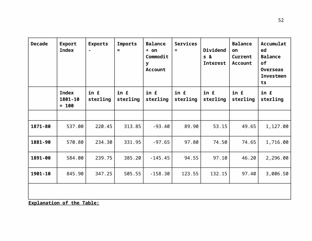
Table 2. British Foreign Trade Components, 1801/10 - 1901/10

Decennial Means of British Exports, Imports, "Invisible" Earnings, Balances on Current Account, and Accumulated Balances of Overseas Investments, in Millions of Pounds Sterling, in Current Prices

Decade ExportIndex

Exports - Imports = Balance + on Commodity Account

Services + Dividends & Interest

Balance on Current Account

Accumulated Balance of Overseas Investments

Index1801-10 = 100

in £ sterling in £ sterling in £ sterling in £ sterling in £ sterling in £ sterling in £ sterling

1801-10 100.00 41.05 50.95 -9.90

1811-20 101.30 41.60 49.80 -8.20

1821-30 89.20 36.60 47.05 -10.45 12.40 4.40 6.35 104.50

1831-40 110.00 45.15 63.70 -18.55 16.35 6.70 4.50 149.50

1841-50 140.00 57.45 79.35 -21.90 18.70 8.50 5.30 197.00

36

Decade ExportIndex

Exports - Imports = Balance + on Commodity Account

Services + Dividends & Interest

Balance on Current Account

Accumulated Balance of Overseas Investments

Index1801-10 = 100

in £ sterling in £ sterling in £ sterling in £ sterling in £ sterling in £ sterling in £ sterling

1851-60 259.60 106.55 137.20 -30.65 33.60 14.10 17.05 314.50

1861-70 404.60 166.10 223.60 -57.50 62.50 26.30 31.30 591.00

1871-80 537.00 220.45 313.85 -93.40 89.90 53.15 49.65 1,127.00

1881-90 570.80 234.30 331.95 -97.65 97.80 74.50 74.65 1,716.00

1891-00 584.00 239.75 385.20 -145.45 94.55 97.10 46.20 2,296.00

1901-10 845.90 347.25 505.55 -158.30 123.55 132.15 97.40 3,006.50

Explanation of the Table:

37

Subtract imports from exports to obtain the balance on the commodity account, which was always negative (i.e. the British imported a greater value of goods than they exported). To that negative balance on the commodity account, add the "invisibles" consisting of "services" (i.e. shipping, banking, insurance revenues, etc.) and those dividends and interest payments received on foreign (overseas) investments, in order to obtain the final balance on Current Account, which was always positive. Gold movements and other items on Capital Account are not shown here.

The Equation: Exports - Imports = Balance on the Commodity Account + Services + Dividends & Interest = Balance on the Current Account.

* The accumulated net balance of overseas investments (foreign credits) includes the retained or re-invested interest and dividends on accumulated foreign investments. Gold movements and other items on the capital account are not given.

Source: Calculated from Peter Mathias, First Industrial Nation (London, 1969), Table VII, p. 305.

38

Table 3.Capital Investments, Domestic and Foreign, in the British Economy,

1870-4 to 1910-14

Net Domestic Capital Formation and Net Foreign Investments,in Millions of Pounds Sterling, Current Values,

and as Percentages of Net National Product:

Quinquennial Means, 1870 - 1914 Period Net Net N.D.C.F. Net N.F.I. Total National Domestic as % Foreign as % Investment

Product Capital of Invest- of as % of in Formation NNP ment in NNP NNPMillions Millions Millions £ £ £

1870-4 1,020.6 26.6 2.6% 78.4 7.7% 10.3%

1875-9 1,036.8 48.6 4.7% 30.4 2.9% 7.6%

1880-4 1,080.8 32.4 3.0% 54.6 5.1% 8.0%

1885-9 1,153.4 14.2 1.2% 80.4 7.0% 8.2%

1890-4 1,307.4 29.0 2.2% 69.8 5.3% 7.5%

1895-9 1,503.8 66.8 4.4% 44.4 3.0% 7.4%

1900-4 1,671.6 109.2 6.5% 34.4 2.1% 8.6%

1905-9 1,833.0 57.4 3.1% 132.6 7.2% 10.4%

1910-4 2,107.4 36.0 1.7% 190.0 9.0% 10.7%

Source: Charles H. Feinstein, Statistical Tables of National Income, Expenditure and Output of the U.K., 1855-1965 (Cambridge, 1976), pp. T-4, 5, T-37, 38; T-106, 107.

39

Table 4 Net Capital Formation (Domestic and Foreign) as a Percentage of Net National

Product in Germany and the U.K.: 1860-1910

Decade Germany U.K. U.K.

(Mitchell (Kuznets (Feinstein 1975) 1961) 1976)

1860-9 11.9% 10.0% -

1870-9 12.1% 11.8% 8.9%

1880-9 11.1% 10.9% 8.1%

1890-9 13.6% 10.1% 7.5%

1900-9 14.4% 11.7% 9.5%

40

Table 5: Capital Formation Ratios in the UK and Germany, 1865 - 1904

in current nominal values and in constant 1913 values

Years UK:NDCF/NDPcurrent values

UK: NDCF/NDPconstant values

UK: NNCF/NNPcurrent values

UK: NNCF/NNPconstant values

Germ-anyNDCF/NDP current

Germ-anyNNCF/NNP current

Germ-anyNNCF/NNP constant

1860-1870

7.20 8.60 10.00 11.50 8.50 9.70 10.60

1870-1880

8.20 7.30 11.80 10.90 11.60 13.50 13.00

1880-1890

6.40 3.40 10.90 8.10 11.20 14.00 14.50

1890-1900

7.30 3.00 10.10 6.00 13.90 15.40 15.90

1900-1910*

8.80 4.80 10.50 6.70 15.60 16.50 15.90

* For the UK: 1895-1904; for Germany: 1901-13

NDCF/NDP: Net Domestic Capital Formation as a Percentage of Net Domestic ProductNNCF/NNP: Net National Capital Formation (Total) as a Percentage of Net National Product

Source:

Y. Goo Park, ‘Depression and Capital Formation: the United Kingdom and Germany, 1873 - 1896’, Journal of European Economic History, 26:3 (Winter 1997), p.514

Table 6. United Kingdom

Average Annual Growth Rates (% p.a.)

Period Manufacturing Gross Domestic Product & Mining (1907 Prices)

1853-1873 2.7% 1.95%

1873-1883 2.2% 1.90%

1883-1899 2.1% 1.85%

1899-1913 2.0% 1.70%

Source: W.A. Lewis, Growth and Fluctuations, 1870-1913 (1978)

Table 7. Average Annual Rates of Real Growth

in the United Kingdom, 1855 - 1913

Period No. Total Real Gross Domestic ProductYears Industrial at Constant Factor Prices

Output (at (from output data)constant price)

1855-69 15 2.08% 1.63%

1870-84 15 2.04% 1.71%

1885-99 15 2.91% 2.14%

1900-13 14 1.60% 1.64%

......................................................

1855-1913 59 2.29% 1.87%

1870-1913 44 2.09% 1.82%

Source: Charles Feinstein, Statistical Tables of National Income, Expenditure, and Output of the United Kingdom, 1855-1965 (1976)

Table 8. Aggregate and Per Capita Indices of IndustrialProduction (United Kingdom in 1900 = 100), and percentageshares of World Industrial Production, for variouscountries: in 1860 and 1913

Country Total Per Capita Percentage Shares ofIndustrial Industrial World IndustrialOutput Output Production

With 1913 1860 1913 1860 1913 1860 1913Frontiers Index Index Index Index % %

UnitedKingdom* 45 127 64 115 20% 14%

Germany 11 138 15 85 5% 15%

France 18 57 20 59 8% 6%

Russia 16 77 8 20 7% 8%

ALL EUROPE 120 528 17 45 53% 57%

UnitedStates 16 298 21 126 7% 32%

Canada 1 9 7 46 -- 1%

Source: Paul Bairoch, ‘International Industrialization Levels from 1760 to 1980,’ Journal of European Economic History, 11 (Fall 1982), 269-333, tables 4 - 13.

* The United Kingdom of Great Britain and Ireland: the values for its aggregate and per capita industrial outputs for 1900 are taken as the base 100 for all the indices in columns 1 to 4. Note that columns 5 and 6 are percentages of total world industrial output.

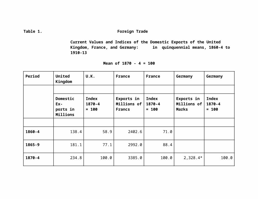
Table 9. Indices of Industrial Output*: in the United Kingdom, France, Germany, and the United States in quinquennial means, 1860-4 to 1910-13

Mean of 1870-4 = 100

Period United France Germany United Kingdom States

1860-64 72.6

1865-69 82.8 95.8 72.6 75.5

1870-74 100.0 100.0 100.0 100.0

1875-79 105.5 109.5 120.8 111.4

1880-84 123.4 126.6 160.6 170.4

1885-89 129.5 130.3 194.9 214.9

1890-94 144.2 151.5 240.6 266.4

1895-99 167.4 167.8 306.4 314.2

1900-04 181.1 176.1 354.3 445.7

1905-09 201.1 206.2 437.4 570.0

1910-13 219.5 250.2 539.5 674.9

* Excluding construction, but including building materials.

Source: W. Arthur Lewis, Growth and Fluctuations, 1870 - 1913 (London, 1978), pp. 248-50, 269, 271, 273.

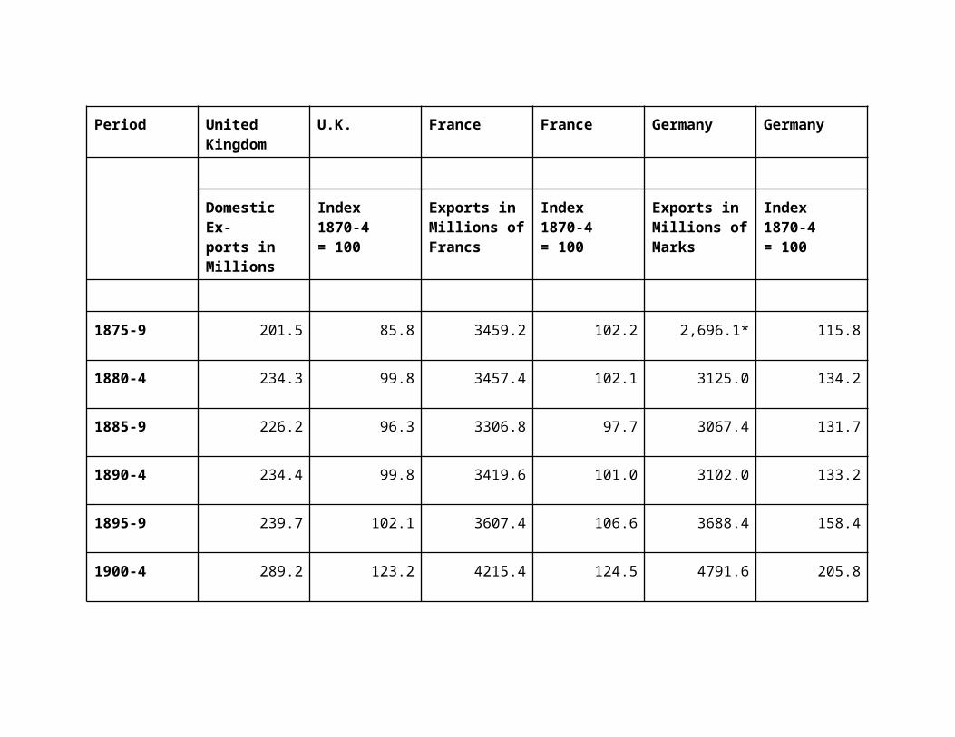
Table 10 Real Gross Domestic Product per Worker

in the United Kingdom, 1856 - 1913

Average Annual Percentage Rates of Growth

Period Income Expenditure Output

1856 - 73 1.32 1.38 1.12

1873 - 82 0.90 1.03 1.20

1882 - 99 1.49 1.27 0.85

1899 - 1913 0.09 0.33 0.72

...................................................................

1856 - 1882 1.18 1.26 1.15

1882 - 1913 0.86 0.84 0.79

1856 - 1913 1.01 1.03 0.95

.................................................................

Source: Charles Feinstein, ‘What Really Happened to Real Wages: Trends in Wages, Prices, and

Productivity in the United Kingdom, 1880 - 1913,’ Economic History Review, 2nd ser. 43

(August 1990).

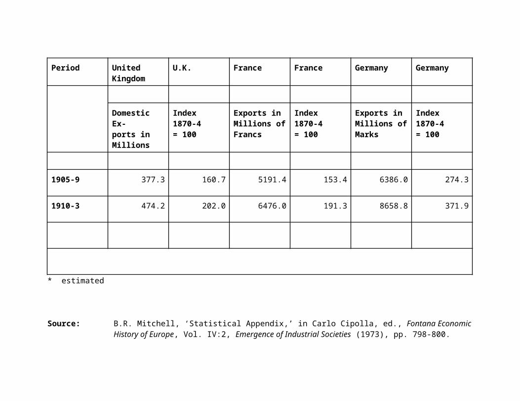
Table 11: Indices of Industrial Output and of Unemployment in the British Economy,

1851 - 60 to 1926 - 30

Mean of Industrial Outputs, 1920 - 1938 = 100

Index Numbers of Industrial Employment and

Trade Union Unemployment Rates in Great Britain

1851 - 1938, in five year means

Beveridge Pigou

Date Construction Textiles Other All Unemploy- Unemploy-

Industries Industries ment Rate ment Rate

1851-55 3.98

1856-60 98.06 106.08 102.08 101.56 3.86 5.66

1861-65 105.20 79.16 100.84 97.06 3.64 4.88

1866-70 96.28 95.44 102.90 98.12 5.08 5.84

1871-75 107.70 109.00 107.02 107.84 1.51 1.56

1876-80 96.74 99.58 104.18 100.14 6.00 6.42

1881-85 105.76 101.00 104.06 103.74 4.84 5.16

1886-90 96.16 102.28 98.04 98.62 5.00 5.38

1891-95 93.80 100.88 94.10 95.30 6.10 6.00

1896-00 104.70 101.36 97.20 101.16 2.85 2.78

1901-05 101.20 94.00 96.24 97.34 4.84 4.60

Index Numbers of Industrial Employment and

Trade Union Unemployment Rates in Great Britain

1851 - 1938, in five year means

Beveridge Pigou

Date Construction Textiles Other All Unemploy- Unemploy-

Industries Industries ment Rate ment Rate

1906-10 96.54 99.16 100.90 98.80 6.02 5.50

1911-15 103.73 105.73 101.80 103.70 2.51 2.52

1916-20 1.36

1921-25 102.20 101.94 100.70 100.24 13.08

Source: William Beveridge, Full Employment in a Free Society, 2nd edn (London, 1960), Appendix A: ‘Trade Union Unemployment Rate, ’ pp. 312-13; Arthur Pigou, Industrial Fluctuations (London, 1927), pp. 353-54.

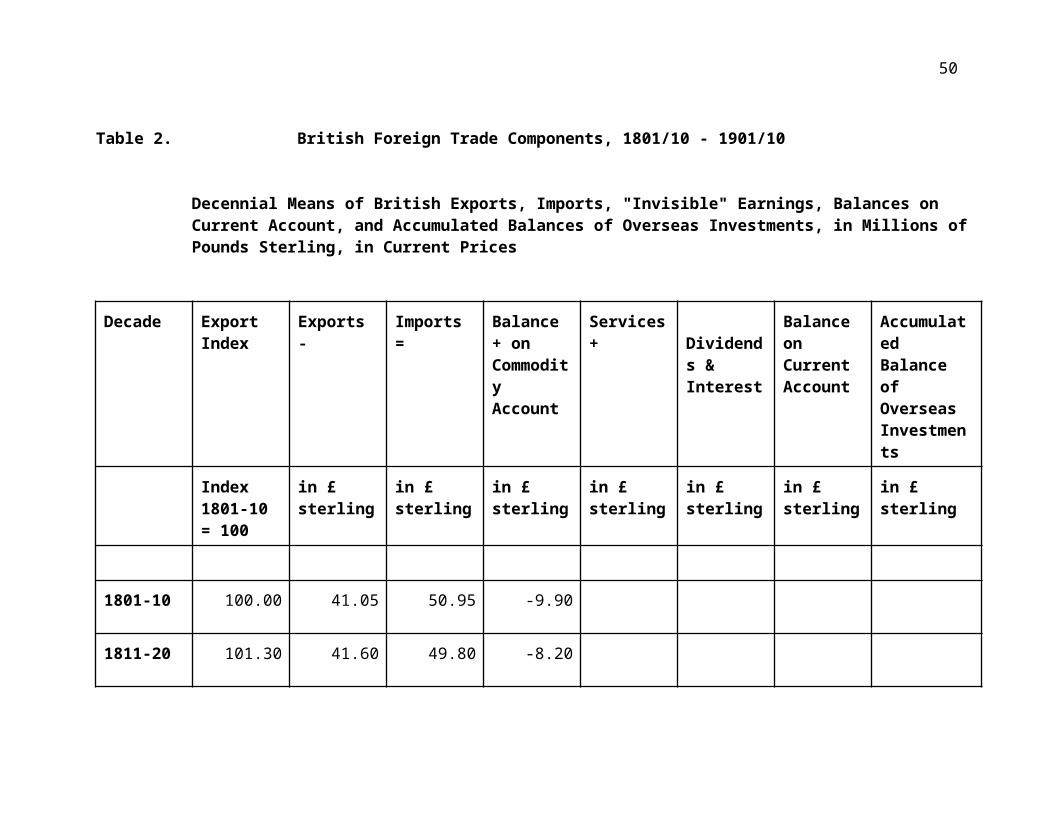
Table 12: Per Capita Product in Selected

European Countries, 1850 - 1910:

Measured in Constant 1970 U.S. Dollars

COUNTRY 1850 1870 1890 1910 Percent-age Total Growth1850-1910

BRITAIN 660 904 1,130 1,302 197%

FRANCE 432 567 668 883 204%

GERMANY 418 579 729 958 229%

BELGIUM 534 738 932 1,110 208%

NETHER-LANDS

481 591 768 952 198%

Source: Nicholas Crafts, ‘Gross National Product in Europe, 1870 - 1910: Some New Estimates,’ Explorations in Economic History, 20 (October 1983), 387-401.

Table 13: International Acceptance Banking by Britishand Continental Banks in 1900 and 1913

in Millions of Pounds Sterling

Name of the Bank Date Founded

1900: Acceptances in £ millions

1913: Acceptances in £ millions

London Merchant Banks:* German origin + Dutch origin ++ U.S. origin

Kleinwort, Sons & Co.* 1796 8.2 13.6

J. Henry Schröder & Co.* 1815 5.9 11.6

Baring Bros & Co. Ltd.+ 1763 3.9 6.6

Brown, Shipley & Co.++ 1805 n.d. 5.1

W. Brandt's Sons & Co.* 1805 1.2 3.3

N.M. Rothschild & Sons * 1798 1.5 3.2

C.J. Hambro & Son* 1800 1.9 3.0

British Joint Stock Banks

London Country & Westminster 1834 0.2 7.8

Union of London & Smiths Bank 1839 3.1 5.8

Parr's Bank 1865 2.4 5.4

London Joint Stock Bank 1836 1.4 3.2

Manchester & Liverpool District 1829 1.7 2.7

Glyn, Mills, and Co. 1753 1.2 1.4

Continental Banks

Dresdner Bank 1872 6.1 14.4

Discontogesellschaft 1851 3.0 12.5

Crédit Lyonnais 1863 0.0 5.7

Russian Bank of Foreign Trade 1871 2.2 3.7

Credito Italiano 1870 n.d. 1.9

Source: Stanley Chapman, The Rise of Merchant Banking (London, 1984), Table 7.2, p. 121.

Table 14. London Merchant Banks: Issuance of U.S. and CanadianRailroad Stocks, 1865 - 1890

Name of the Merchant Bank Value of Issues in £ millions

Percentage of Total Issues

Baring Bros 34.68 28.7%

J.S. Morgan * 26.09 21.6%

Bischoffsheim & Goldschmidt 10.17 8.4%

Morton, Rose & Co.* 9.48 7.8%

Speyer Bros. * 9.16 7.6%

Brown, Shipley & Co. ** 6.39 5.2%

Robert Benson & Co. 6.07 5.0%

Jay Cooke, McCulloch & Co. * 5.12 4.2%

L. Cohen & Sons 2.31 1.9%

Union Bank of London (Schuster) 2.24 1.9%

Thomson, Bonar & Co. 2.00 1.7%

J.H. Schröder & Co. 1.85 1.5%

R. Raphael & Sons 1.50 1.2%

Seligman & Co. * 1.40 1.2%

N.M. Rothschild & Sons 0.80 0.7%

C. de Murrieta & Co. 0.55 0.5%

C.J. Hambro & Sons 0.50 0.4%

Henry S. King & Co. * 0.45 0.4%

Jay & Co. * 0.10 0.1%

TOTAL of 19 merchant banks 120.86 100.0%

* Branch of a U.S. banking house ** U.S. origins

Source: Stanley Chapman, The Rise of Merchant Banking (1984), p. 97.

Table 15. Banking Structures in England & Wales and the United Kingdom

EW: England and Wales

UK: United Kingdom (England, Wales, Scotland, and Ireland)

PB: private partnership banks

JSB: joint-stock banks

Year EW: Private Banks

EW: PB Offices/Branches

EW:Joint-Stock Banks

EW: JSBOffices/Branches

UK:Total Banks

UK:Total Offices/Branches

UK: Average No. of Branches

1850 327 518 99 576 459 1,685 3.67

1875 236 595 122 1,364 381 3,320 8.71

1900 81 358 83 4,212 184 6,269 34.07

1913 29 147 41 6,426 88 8,610 97.84

Table 16: English Commercial Banking Asset Ratios (percentages)

Years Private Sector Loans

Advances Bills Investments Cash

1860 69.4 46.7 30.7 16.2 13.1

1870 75.9 49.0 33.6 13.3 13.8

1880 65.1 47.6 20.0 17.7 19.2

1890 62.6 50.1 15.7 18.5 17.8

1900 57.0 50.6 11.1 22.8 18.7

1910 54.0 48.0 10.2 22.0 22.2

1913 55.6 46.8 12.0 17.9 24.6

Source: Mae Baker and Michael Collins, ‘Financial Crises and Structural Change in English Commercial Bank Assets, 1860 - 1913’, Explorations in Economic History, 26:4 (October 1999), 428-44.

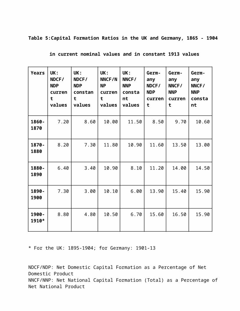
Table 17. World Gold Mining Outputs in the 19th Century, 1850 - 1913Average Annual Gold Outputs in Metric Tonnes

Decade Australia New Zealand Russia South Africa Rhodesia Mexico Canada United States World Total Total in kg.

1850-976.8 0.3 25.4 83.4 185.9 185,900

1860-961.9 14.1 25.1 70.6 171.7 171,700

1870-946.0 12.0 37.1 1.6 61.5 158.2 158,200

1880-935.8 6.7 34.8 4.5 1.6 2.0 49.6 135.0 135,000

1890-959.7 8.4 38.4 62.0 1.2 8.0 7.7 70.2 255.6 255,600

1900-1494.6 13.4 39.9 171.2 14.6 25.1 22.8 132.3 513.9 513,900

Totals374.8 54.9 200.7 237.7 15.8 36.3 32.5 467.6 1,420.3 1,420,300

Percent26.4% 3.9% 14.1% 16.7% 1.1% 2.6% 2.3% 32.9% 100.0%

Sources:C.J. Schmitz, World Non-Ferrous Metal Production and Prices, 1700-1976 (London, 1979).

Barry Eichengreen and Ian McLean, ‘The Supply of Gold under the Pre-1914 Gold Standard,’ Economic History Review, 2nd ser. 47:2 (May 1994).

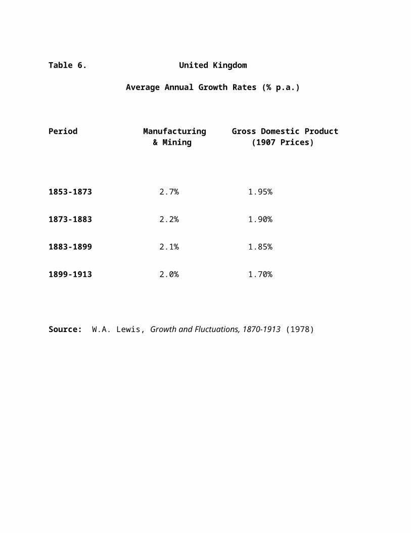
Table 18 Money Supply, GDP, and Prices in Canada, 1955 - 2007: Annual Means of monthly data

M: MB V k P y GDP = Y Population Inflation:= Y/M Gross

DomesticYear Money: Income Cambridge CPI Real GDP: Product in Canadian Percent Bank Real GDP

Monetary Velocity cash June 1992= in billions of billions population Change Rate perBase in of M: balances 100.00 1992 dollars current in millions in CPI in percent capitabillions Mon Base k = 1/V CANSIM CANSIM market in dollars

pricesCANSIM

1955 2.2588 16.83 15,681,250 1.8961956 2.3793 17.07 16,070,250 1.39% 3.1531957 2.4378 17.60 16,579,500 3.12% 4.0231958 2.5973 18.04 17,062,250 2.51% 2.4991959 2.7276 18.25 17,467,500 1.15% 5.1281960 2.7500 18.48 17,855,250 1.23% 3.5391961 2.8565 14.414 0.06938 18.70 220.176 41.1730 18,224,500 1.22% 3.061 12,081.341962 3.0239 14.771 0.06770 18.87 236.740 44.6650 18,570,750 0.89% 4.477 12,748.021963 3.1361 15.293 0.06539 19.22 249.561 47.9610 18,919,000 1.86% 3.875 13,191.001964 3.3160 15.847 0.06310 19.57 268.564 52.5490 19,277,250 1.81% 4.042 13,931.651965 3.5971 16.105 0.06209 20.03 289.288 57.9300 19,633,500 2.34% 4.292 14,734.431966 3.8743 16.730 0.05977 20.78 311.875 64.8180 19,997,500 3.79% 5.167 15,595.691967 4.1888 16.639 0.06010 21.53 323.675 69.6980 20,363,750 3.61% 4.979 15,894.661968 4.2691 17.833 0.05608 22.39 339.997 76.1310 20,692,000 3.99% 6.792 16,431.331969 4.7133 17.785 0.05623 23.43 357.717 83.8250 20,994,250 4.65% 7.458 17,038.801970 4.9789 18.112 0.05521 24.21 372.512 90.1790 21,287,500 3.31% 7.125 17,499.111971 5.5635 17.692 0.05652 24.87 395.827 98.4290 21,747,314 2.72% 5.188 18,201.191972 6.3914 17.197 0.05815 26.08 421.392 109.9130 22,187,140 4.89% 4.750 18,992.611973 7.3540 17.535 0.05703 28.06 459.600 128.9560 22,453,775 7.57% 6.125 20,468.701974 8.3454 18.458 0.05418 31.13 494.769 154.0380 22,772,045 10.96% 8.500 21,727.021975 9.7236 17.856 0.05600 34.46 503.858 173.6210 23,102,980 10.68% 8.500 21,809.211976 10.9117 18.328 0.05456 37.06 539.673 199.9940 23,414,365 7.55% 9.292 23,048.821977 12.0083 18.402 0.05434 40.03 552.087 220.9730 23,694,035 8.01% 7.708 23,300.69

Table 18 Money Supply, GDP, and Prices in Canada, 1955 - 2007: Annual Means of monthly data

M: MB V k P y GDP = Y Population Inflation:= Y/M Gross

DomesticYear Money: Income Cambridge CPI Real GDP: Product in Canadian Percent Bank Real GDP

Monetary Velocity cash June 1992= in billions of billions population Change Rate perBase in of M: balances 100.00 1992 dollars current in millions in CPI in percent capitabillions Mon Base k = 1/V CANSIM CANSIM market in dollars

prices1978 13.4578 18.196 0.05496 43.61 561.537 244.8770 23,935,651 8.95% 8.979 23,460.281979 14.8698 18.802 0.05319 47.59 587.449 279.5770 24,170,445 9.13% 12.104 24,304.451980 16.0130 19.633 0.05093 52.43 599.695 314.3900 24,471,129 10.16% 12.891 24,506.221981 17.1964 20.962 0.04771 58.94 611.572 360.4710 24,785,059 12.43% 17.931 24,675.051982 17.4193 21.807 0.04586 65.31 581.639 379.8590 25,083,479 10.80% 13.958 23,188.151983 17.7398 23.190 0.04312 69.13 595.062 411.3860 25,336,505 5.86% 9.553 23,486.341984 17.9203 25.088 0.03986 72.11 623.481 449.5820 25,577,353 4.30% 11.312 24,376.301985 18.7576 25.894 0.03862 74.97 647.907 485.7140 25,813,854 3.96% 9.647 25,099.181986 19.9900 25.640 0.03900 78.10 656.262 512.5410 26,068,353 4.18% 9.214 25,174.681987 21.0964 26.495 0.03774 81.49 685.897 558.9490 26,399,956 4.34% 8.403 25,981.001988 22.2465 27.559 0.03629 84.79 723.059 613.0940 26,754,940 4.05% 9.686 27,025.261989 23.5343 27.948 0.03578 89.03 738.813 657.7280 27,219,748 4.99% 12.293 27,142.531990 24.4104 27.854 0.03590 93.27 729.008 679.9210 27,638,583 4.76% 13.045 26,376.441991 25.3470 27.039 0.03698 98.51 695.745 685.3670 27,987,829 5.62% 9.034 24,858.851992 26.7329 26.203 0.03816 99.98 700.655 700.4800 28,319,473 1.49% 6.783 24,741.111993 28.2746 25.719 0.03888 101.83 714.092 727.1840 28,648,235 1.86% 5.088 24,926.221994 29.2574 26.348 0.03795 102.00 755.758 770.8730 28,958,270 0.16% 5.766 26,098.171995 29.5420 27.433 0.03645 104.21 777.698 810.4260 29,262,649 2.17% 7.308 26,576.471996 30.1993 27.711 0.03609 105.85 790.613 836.8640 29,570,577 1.58% 4.531 26,736.481997 31.7384 27.813 0.03595 107.57 820.638 882.7330 29,868,726 1.62% 3.521 27,474.831998 33.5764 27.250 0.03670 108.63 842.258 914.9730 30,125,715 0.99% 5.104 27,958.111999 36.5423 26.885 0.03720 110.52 888.953 982.4410 30,369,575 1.73% 4.917 29,271.162000 38.1102 28.223 0.03543 113.53 947.357 1,075.5660 30,650,631 2.73% 5.771 30,908.242001 39.6666 27.919 0.03582 116.41 951.357 1,107.4590 30,973,522 2.53% 4.313 30,715.172002 42.3101 27.280 0.03666 119.03 969.716 1,154.2040 31,322,332 2.25% 2.708 30,959.242003 43.9059 27.700 0.03610 122.32 994.297 1,216.1910 31,626,552 2.77% 3.188 31,438.68

Table 18 Money Supply, GDP, and Prices in Canada, 1955 - 2007: Annual Means of monthly data

M: MB V k P y GDP = Y Population Inflation:= Y/M Gross

DomesticYear Money: Income Cambridge CPI Real GDP: Product in Canadian Percent Bank Real GDP

Monetary Velocity cash June 1992= in billions of billions population Change Rate perBase in of M: balances 100.00 1992 dollars current in millions in CPI in percent capitabillions Mon Base k = 1/V CANSIM CANSIM market in dollars

prices2004 45.2319 28.524 0.03506 124.56 1,035.808 1,290.1850 31,932,015 1.83% 2.500 32,437.912005 47.3058 28.991 0.03449 127.34 1,076.965 1,371.4250 32,258,138 2.23% 2.917 33,385.842006 49.6239 29.145 0.03431 129.90 1,113.400 1,446.3070 32,603,606 2.01% 4.313 34,149.612007 52.1695 29.436 0.03397 131.65 1,166.461 1,535.6460 32,881,904 1.35% 4.604 35,474.26

Money Source Definition

Monetary Base CANSIM notes and coin in circulation, chartered bank and other Canadian Payments Association members' deposits with the Bank of Canada

M1 IMF notes, coins, chequable deposits: narrowly defined

M1B CANSIM currency outside banks, chartered bank chequable deposits, less inter-bank chequable deposits

M1+ Gross IMF M1 broadly defined: notes, coins, chequable and other deposits; Canada Savings Bond and other liquid assets