U.S. Department of the InteriorU.S. Geological Survey

Data Series 901

Mount St. Helens—Controlled-Source Audio-Frequency Magnetotelluric (CSAMT) Data and Inversions

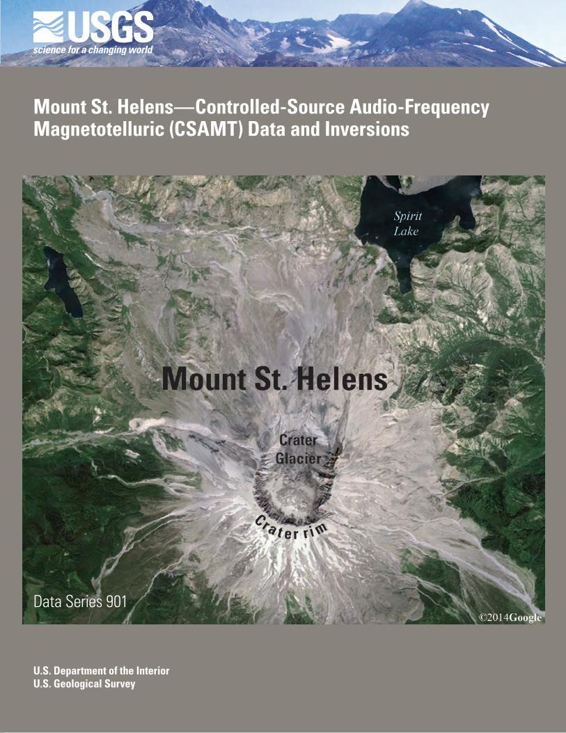
Cover. A Google Earth image taken in 2014 of Mount St. Helens, Washington.

Mount St. Helens—Controlled-Source Audio-Frequency Magnetotelluric (CSAMT) Data and InversionsBy Jeff Wynn and Herbert A. Pierce

Data Series 901

U.S. Department of the InteriorU.S. Geological Survey

U.S. Department of the InteriorSALLY JEWELL, Secretary

U.S. Geological SurveySuzette M. Kimball, Acting Director

U.S. Geological Survey, Reston, Virginia: 2015

For more information on the USGS—the Federal source for science about the Earth, its natural and living resources, natural hazards, and the environment—visit http://www.usgs.gov or call 1–888–ASK–USGS.

For an overview of USGS information products, including maps, imagery, and publications, visit http://www.usgs.gov/pubprod/..

Any use of trade, firm, or product names is for descriptive purposes only and does not imply endorsement by the U.S. Government.

Although this information product, for the most part, is in the public domain, it also may contain copyrighted materials as noted in the text. Permission to reproduce copyrighted items must be secured from the copyright owner.

Suggested citation:Wynn, Jeff, and Pierce, H.A., 2015, Mount St. Helens—controlled-source audio-frequency magnetotelluric (CSAMT) data and inversions: U.S. Geological Survey Data Series 901, 8 p., http://dx.doi.org/10.3133/ds901.

ISSN 2327-638X (online)

iii

Contents

Introduction.....................................................................................................................................................1Data Acquisition .............................................................................................................................................12010...................................................................................................................................................................42011...................................................................................................................................................................4Data Processing .............................................................................................................................................4Assigning TE and TM directions..................................................................................................................4Occam Inversions ..........................................................................................................................................4Fischer Inversions..........................................................................................................................................5Marquardt Inversions....................................................................................................................................5References Cited............................................................................................................................................8

Figures 1. A Google Earth image of Mount St. Helens, showing the controlled-source audio-

frequency magnetotelluric (CSAMT) station locations ..........................................................2 2. Images showing data acquisition ................................................................................................3 3. Example of an Occam inversion of controlled-source audio-frequency magnetotelluric

(CSAMT) data .....................................................................................................................................5 4. Example of a Fischer Inversion of the controlled-source audio-frequency

magnetotelluric (CSAMT) data ...................................................................................................6 5. Example of a Marquardt Inversion of the controlled-source audio-frequency

magnetotelluric (CSAMT) data ...................................................................................................7

Tables 1. GPS coordinates and elevations for the controlled-source audio-frequency

magnetotelluric (CSAMT) stations acquired in and adjacent to Mount St. Helens, Washington. (Datum: WGS 84) ...................................................................................................3

IntroductionThis report describes a series of geoelectrical

soundings carried out on and near Mount St. Helens volcano, Washington, in 2010–2011. These soundings used a controlled-source audio-frequency magnetotelluric (CSAMT) approach (Zonge and Hughes, 1991; Simpson and Bahr, 2005). We chose CSAMT for logistical reasons: It can be deployed by helicopter, has an effective depth of penetration of as much as 1 kilometer, and requires less wire than a Schlumberger sounding.

This Data Series provides the edited data for these CSAMT soundings as well as several different types of 1-D inversions (where the signal data are converted to conductivity-versus-depth models). In addition, we include a map showing station locations on and around the volcano and the Pumice Plain to the north.

The apparent conductivity (or its inverse, apparent resistivity) measured by a geoelectrical system is caused by several factors. The most important of these are water-filled rock porosity and the presence of water-filled fractures; however, rock type and minerals (for instance, sulfides and clay content) also contribute to apparent conductivity. In situations with little recharge (for instance, in arid regions), variations in ionic content of water occupying pore space and fractures sampled by the measurement system must also be factored in (Wynn, 2006). Variations in ionic content may also be present in hydrothermal fluids surrounding volcanoes in wet regions. In unusual cases, temperature may also affect apparent conductivity (Keller, 1989; Palacky, 1989). There is relatively little hydrothermal alteration (and thus fewer clay minerals that might add to the apparent conductivity) in the eruptive products of Mount St. Helens (Reid and others, 2010), so conductors observed in the Fischer, Occam, and Marquardt inversion results later in this report are thus believed to map zones with significant water content. Geoelectrical surveys thus have the potential to reveal subsurface regions with significant groundwater content, including perched and regional aquifers. Reid and others (2001) and Reid (2004) have suggested that groundwater involvement may figure in both the scale

Mount St. Helens—Controlled-Source Audio-Frequency Magnetotelluric (CSAMT) Data and Inversions

By Jeff Wynn and Herbert A. Pierce

and the character of some if not all volcanic edifice collapse events. Ongoing research by the U.S. Geological Survey (USGS) and others aims to better understand the contribution of groundwater to both edifice pore pressure and rock alteration as well as its direct influence on eruption processes by violent interaction with magma (Schmincke, 1998).

Data AcquisitionThe CSAMT soundings were carried out using

a Geometrics Stratagem EH-4 system on and near Mount St. Helens in 2010 and 2011. In all cases save one (station MSH-1102, where a natural-source audio-frequency magnetotelluric [NSAMT] approach was used), a controlled-source inductive transmitter was used to improve the quality of the received signal. The transmitter substantially improves the signal/noise ratio and thus shortens the time required for a measurement. Station MSH-1102 (NSAMT) was repeated using a controlled-source electromagnetic transmitter, with station MSH-1110 (CSAMT) measured subsequently as a quality check. The transmitter was always located approximately 250 meters away from each receiver location to maximize signal quality, but also to avoid near-field distortion effects. The transmitter was only needed to augment the weak mid-band natural signals (450–2,700 Hz), so we acquired preliminary bulk resistivity data and used the Stratagem EH-4 manual (Geometrics, 2007, fig. 5) to calculate skin-depth and guide us on where to place the transmitter. We used high-sensitivity EMI Corporation magnetic coils and orthogonal, 25-meter electric dipoles. The latter were coupled to porous-pot ceramic, non-polarizing electrodes, as sensors. The CSAMT station locations are shown in figure 1, and the station coordinates and elevations are provided in the “GPS Data” section (table 1). Photographs of the CSAMT equipment are shown in figure 2. A Long Ranger (Bell 206L) helicopter was used for access to all stations, with permission of the Mount St. Helens National Volcanic Monument. Two load trips were required for each station.

2 Mount St. Helens—Controlled-Source Audio-Frequency Magnetotelluric (CSAMT) Data and Inversions

Spirit Lake

CastleLake

0

0 2 MILES

3 KILOMETERS

P u m i c e

P l a i n

1106

1105

1104step scarp

11031103,1004

11101106,1101,1002

1109

MSH-site number

1107

1108

©2014Google

North Fork Toutle River

Figure 1. A Google Earth image of Mount St. Helens, showing the controlled-source audio-frequency magnetotelluric (CSAMT) station locations. The step scarp, a pronounced topographic offset (north side down), is shown as a blue line.

Data Acquisition 3

Figure 2. Images showing data acquisition. A, The controlled-source audio-frequency magnetotelluric (CSAMT) transmitter for repeat station MSH-1001-1002, located north of Crater Glacier (black ridge visible in the middle distance) and the 1980–86 and 2004–2008 dacite lava domes (left upper background) inside Mount St. Helens crater (crater walls seen in the top center and upper right). USGS photograph by Jeff Wynn. B, The first author with the Stratagem EH-4 controlled-source audio-frequency magnetotelluric (CSAMT) receiver and the electrodes used for the electrical-field measurements. The location here is station MSH-1001-1002, just north of Crater Glacier (seen in the background behind the umbrella). USGS photo by Tami Christensen.

Table 1. GPS coordinates and elevations for the controlled-source audio-frequency magnetotelluric (CSAMT) stations acquired in and adjacent to Mount St. Helens, Washington. (Datum: WGS 84)

StationUTM zone 10N

Latitude LongitudeSurface elevation

Northing Easting (ft) (m)

2010

MSH-1001/2 5117961 562593 46.212 -122.189 5570 1698MSH-1003/4 5118187 562600 46.214 -122.188 5496 1675

2011

MSH-1102 5117948 562577 46.212 -122.189 5597 1706MSH-1103 5118806 562640 46.222 -122.188 5017 1530MSH-1104 5119891 562818 46.232 -122.185 4035 1230MSH-1105 5120906 562821 46.241 -122.185 3762 1147MSH-1106 5122024 562873 46.251 -122.184 3634 1108MSH-1107 5113516 563243 46.174 -122.181 5622 1714MSH-1108 5116637 559491 46.203 -122.229 5004 1526MSH-1109 5116186 564853 46.198 -122.159 6022 1836MSH-1110 5117948 562587 46.212 -122.189 5590 1704

[Coordinates given represent CSAMT receiver locations. The transmitter was located ~250 meters away. Stations 1001/1002 were repeats using the same transmitter-receiver locations. Stations 1003/1004 were repeats using the same transmitter-receiver locations. Stations 1001–1004 were acquired north of and near the toe of the Mount St. Helens Glacier on September 14, 2010. Stations 1102 & 1110 were acquired on separate days using close but not identical transmitter-receiver locations. Stations 1102 & 1110 were acquired very close to the toe of the Mount St. Helens Glacier on September 6 and 7, 2011.]

BA

4 Mount St. Helens—Controlled-Source Audio-Frequency Magnetotelluric (CSAMT) Data and Inversions

2010

The soundings carried out in September 2010 were done as a proof-of-concept experiment. They successfully identified a shallow conductor seen earlier in time-domain electromagnetic (TEM) profiling carried out in 2007 (Bedrosian and others, 2008). The soundings represent two repeat measurements each at two different receiver locations inside the crater, and close to the terminus of the growing Crater Glacier at that time. The double measurements were made to ascertain the precision that we could anticipate during subsequent measurements and inversions of the data. Two different receiver locations (see next section) were utilized with an equidistant transmitter for all four measurements. The 2010 stations are labeled MSH-1001 to MSH-1004.

2011

Additional soundings were carried out in September 2011 in two stages. Environmental conditions were virtually identical both years. The first stage acquired a profile from the terminus of the Crater Glacier to the North Fork Toutle River, crossing and sampling the Pumice Plain in a north-south transect. This profile was designed to map the deep regional aquifer, and to determine what (if any) connection it had to the shallow aquifer observed a year earlier inside the crater. Three additional stations were acquired subsequently on the south, west, and east flanks of the volcanic edifice, plus a repeat station at the north edge of the Crater Glacier. These stations were acquired to ascertain if there was any perched water within the edifice. Stations could not be acquired in the central core of the volcano, in the vicinity of the 1980-86 or 2004-2008 lava domes, as there is no way to make an adequate electrical connection with the ground here due to loose talus and ice. The 2011 stations are labeled MSH-1102 to MSH-1110.

Data Processing

After the CSAMT data were downloaded from the field computer system, they were examined for anisotropy and noise both visually and with software. The data were edited using the WinGLink software package in the following manner: (1) Data were evaluated to ensure that individual phase values were in the correct quadrants. (2) Data curves were smoothed using D+ (the delta function of Parker and Booker, 1996). (3) Data were checked to ensure that the rho (resistivity) values did not rise or fall steeper than 45 degrees in log-log space. The effect of this standard processing is to remove the occasional noise outliers and stack the data for the smoothest possible 1-D model fit. While data quality varied somewhat, it was acceptable. All data are reported and released in this report.

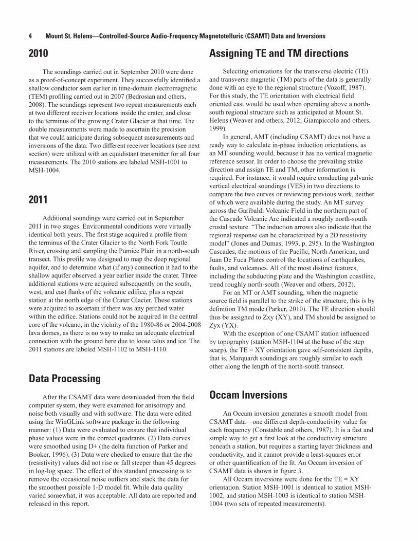
Assigning TE and TM directionsSelecting orientations for the transverse electric (TE)

and transverse magnetic (TM) parts of the data is generally done with an eye to the regional structure (Vozoff, 1987). For this study, the TE orientation with electrical field oriented east would be used when operating above a north-south regional structure such as anticipated at Mount St. Helens (Weaver and others, 2012; Giampiccolo and others, 1999).

In general, AMT (including CSAMT) does not have a ready way to calculate in-phase induction orientations, as an MT sounding would, because it has no vertical magnetic reference sensor. In order to choose the prevailing strike direction and assign TE and TM, other information is required. For instance, it would require conducting galvanic vertical electrical soundings (VES) in two directions to compare the two curves or reviewing previous work, neither of which were available during the study. An MT survey across the Garibaldi Volcanic Field in the northern part of the Cascade Volcanic Arc indicated a roughly north-south crustal texture. “The induction arrows also indicate that the regional response can be characterized by a 2D resistivity model” (Jones and Dumas, 1993, p. 295). In the Washington Cascades, the motions of the Pacific, North American, and Juan De Fuca Plates control the locations of earthquakes, faults, and volcanoes. All of the most distinct features, including the subducting plate and the Washington coastline, trend roughly north-south (Weaver and others, 2012).

For an MT or AMT sounding, when the magnetic source field is parallel to the strike of the structure, this is by definition TM mode (Parker, 2010). The TE direction should thus be assigned to Zxy (XY), and TM should be assigned to Zyx (YX).

With the exception of one CSAMT station influenced by topography (station MSH-1104 at the base of the step scarp), the TE = XY orientation gave self-consistent depths, that is, Marquardt soundings are roughly similar to each other along the length of the north-south transect.

Occam Inversions

An Occam inversion generates a smooth model from CSAMT data—one different depth-conductivity value for each frequency (Constable and others, 1987). It is a fast and simple way to get a first look at the conductivity structure beneath a station, but requires a starting layer thickness and conductivity, and it cannot provide a least-squares error or other quantification of the fit. An Occam inversion of CSAMT data is shown in figure 3.

All Occam inversions were done for the TE = XY orientation. Station MSH-1001 is identical to station MSH-1002, and station MSH-1003 is identical to station MSH-1004 (two sets of repeated measurements).

Marquardt Inversions 5

Figure 3. Example of an Occam inversion of controlled-source audio-frequency magnetotelluric (CSAMT) data. A, The computer inversion of the data into a resistivity versus depth vertical profile for station MSH-1105. B, The original resistivity data and the inversion model fit for resistivity as a function of measurement frequency. C, The original phase data and the inversion model fit for phase as a function of measurement frequency.

100

1,000

10,000

50

500

5,000

1,000

100

10

135

90

45

0

100,000 10,00010,000 1,0001,000 100100 1010

Frequency, in hertz

Phas

e an

gle,

in d

egre

es

Dept

h, in

met

ers

Resis

tivity

, in o

hm-m

eter

s

Resistivity, in ohm-meters

11

EXPLANATION

CSAMT dataat station MSH-1105

Model for TE = XY orientation

Fischer InversionsThe singular advantage of a Fischer-type inversion

is that it does not rely on a starting model. Rather, it makes direct use of the CSAMT data for information regarding layering. A typical use of the Fischer inversion is to determine how many layers can be resolved with the existing data; generally, the layers are visually obvious in the inversion (see fig. 4). These results are then used to help build a Marquardt starting model and then iterated to a true inversion (Fischer and others, 1981; Pedersen and Gharibi, 2000).

All Fischer inversions were done for the TE = XY orientation. Station MSH-1001 is identical to station MSH-1002, and station MSH-1003 is identical to station MSH-1004 (two sets of repeated measurements not duplicated here).

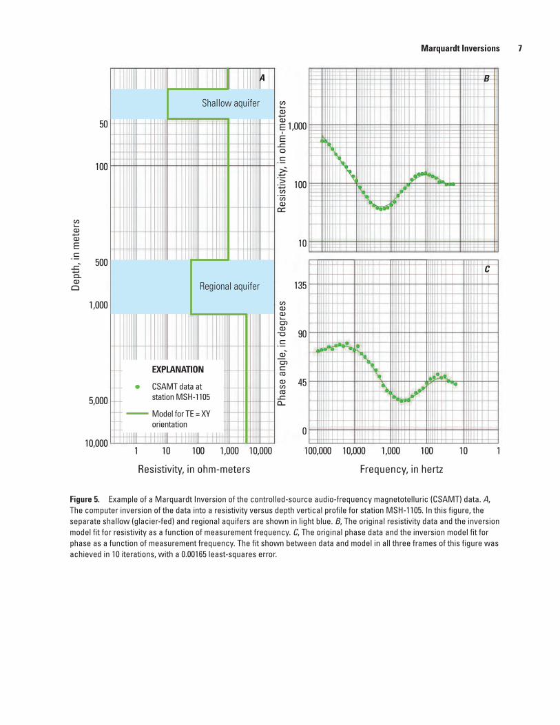
Marquardt Inversions

A Marquardt inversion is a damped, least-squares ridge-regression algorithm used to obtain conductivity versus depth from electromagnetic sounding data (see fig. 5). It requires a starting model that has equal to or less than the number of layers that can reasonably be observed in a Fischer inversion. The algorithm modifies the resistivities and thicknesses of the specified number of layers until it minimizes the least-squares error between the model response and the observed data. It is very sensitive to the starting (initial) model and commonly will not work if one attempts to invert for more layers than are resolved by the data (Marquardt, 1963; Pujol, 2007).

All Marquardt Inversions were done for the TE = XY orientation. If there was apparent anisotropy, the inversion was also done for TE = YX.

A B

C

6 Mount St. Helens—Controlled-Source Audio-Frequency Magnetotelluric (CSAMT) Data and Inversions

Figure 4. Example of a Fischer Inversion of the controlled-source audio-frequency magnetotelluric (CSAMT) data. A, The computer inversion of the data into a resistivity versus depth vertical profile for station MSH-1105. B, The original resistivity data and the inversion model fit for resistivity as a function of measurement frequency. C, The original phase data and the inversion model fit for phase as a function of measurement frequency.

100

1,000

10,000

50

500

5,000

1,000

100

10

1

135

90

45

0

100,000 10,00010,000 1,0001,000 100100 1010

Frequency, in hertz

Phas

e an

gle,

in d

egre

es

Dept

h, in

met

ers

Resi

stiv

ity, i

n oh

m-m

eter

s

Resistivity, in ohm-meters

11

EXPLANATION

CSAMT dataat station MSH-1105

Model for TE = XY orientation

C

BA

Marquardt Inversions 7

Figure 5. Example of a Marquardt Inversion of the controlled-source audio-frequency magnetotelluric (CSAMT) data. A, The computer inversion of the data into a resistivity versus depth vertical profile for station MSH-1105. In this figure, the separate shallow (glacier-fed) and regional aquifers are shown in light blue. B, The original resistivity data and the inversion model fit for resistivity as a function of measurement frequency. C, The original phase data and the inversion model fit for phase as a function of measurement frequency. The fit shown between data and model in all three frames of this figure was achieved in 10 iterations, with a 0.00165 least-squares error.

100

1,000

10,000

50

500

5,000

1,000

100

10

135

90

45

0

100,000 10,00010,000 1,0001,000 100100 1010

Frequency, in hertz

Phas

e an

gle,

in d

egre

es

Dept

h, in

met

ers

Resi

stiv

ity, i

n oh

m-m

eter

s

Resistivity, in ohm-meters

11

EXPLANATION

CSAMT data at station MSH-1105

Model for TE = XY orientation

Shallow aquifer

Regional aquifer

A B

C

8 Mount St. Helens—Controlled-Source Audio-Frequency Magnetotelluric (CSAMT) Data and Inversions

References Cited

Constable, S.C., Parker, R.L., and Constable, C.G., 1987, Occam’s inversion: a practical algorithm for generating smooth models from electromagnetic sounding data: Geophysics, v. 52, no. 3, p. 289–300.

Fischer, G., Schnegg, P.A., Peguiron, M., and LeQuang, B.V., 1981, An analytic one-dimensional magnetotelluric inversion scheme: Geophysical Journal of the Royal Astronomical Society, v. 67, no. 2, p. 257–278.

Geometrics, Inc., 2007, Operation manual for Stratagem [26716–01 rev. F] systems running Imagem ver. 2.19: Geometrics, Inc., 41 p., accessed July 17, 2103, at ftp://geom.geometrics.com/pub/GeoElectric/Manuals/EH4_manual_F.pdf.

Giampiccolo, E., Musumeci, C., Malone, S.D., Gresta, S., and Privitera, E., 1999, Seismicity and stress-tensor inversion in the central Washington Cascade Mountains: Bulletin of the Seismological Society of America, v. 89, no. 3, p. 811–821.

Jones, A.G., and Dumas, I., 1993, Electromagnetic images of a volcanic zone: Physics of the Earth and Planetary Interiors, v. 81, nos. 1–4, p. 289–314.

Kantor, Michael, and Burrows, J.H., 1996, Announcing the standard for electronic data interchange (EDI): National Institute of Standards and Technology, accessed October 11, 2012, at http://www.limswiki.org/index.php/Electronic_data_interchange.

Keller, G.V., 1989, Electrical properties, in Carmichael, R.S., ed., Practical Handbook of Physical Properties of Rocks and Minerals: Boca Raton, Fla., CRC Press, p. 359–427.

Marquardt, Donald, 1963, An algorithm for least-squares estimation of nonlinear parameters: SIAM Journal on Applied Mathematics, v. 11, no. 2, p. 431–441.

Palacky, G.J., 1989, Resistivity characteristics of geologic targets, in Nabighian, M.N., ed., Electromagnetic Methods in Applied Geophysics Theory: Tulsa, Okla., Society of Exploration Geophysics, v. 1, p. 53–129.

Parker, R.L., 2010, Can a 2-D MT frequency response always be interpreted as a 1-D response?: Geophysical Journal International, v. 181, no. 1, p. 269–274.

Parker, R.L., and Booker, J.R., 1996, Optimal one-dimensional inversion and bounding of magnetotelluric apparent resistivity and phase measurements: Physics of the Earth and Planetary Interiors, v. 98, no. 3–4, p. 269–282, doi:10.1016/S0031-9201(96)03191-3.

Pedersen, L.B., and Gharibi, M., 2000, Automatic 1-D inversion of magnetotelluric data—finding the simplest possible model that fits the data: Geophysics, v. 65, no. 3, p. 773–782.

Pujol, Jose, 2007, The solution of nonlinear inverse problems and the Levenberg-Marquardt method: Geophysics, v. 72, no. 4, p. W1–W16.

Reid, M.E., 2004, Massive collapse of volcano edifices triggered by hydrothermal pressurization: Geology, v. 32, no. 5, p. 373–376.

Reid, M.E., Keith, T.E.C., Kayen, R.E., Iverson, N.R., Iverson, R.M., and Brien, D.L., 2010, Volcano collapse promoted by progressive strength reduction—new data from Mount St. Helens: Bulletin of Volcanology, v. 72, no. 6, p. 761–766.

Reid, M.E., Sisson, T.W., and Brien, D.L., 2001, Volcano collapse promoted by hydrothermal alteration and edifice shape, Mount Rainier, Washington: Geology, v. 29, no. 9, p. 779–782.

Schmincke, H.-U., 1998, Volcanism: Berlin, Springer-Verlag, 335 p.

Simpson, Fiona, and Bahr, Karsten, 2005, Practical magnetotellurics: Cambridge, Cambridge University Press, 254 p.

Vozoff, Keeva, 1987, The magnetotelluric method, in Nabighian, M.N., ed., Electromagnetic methods in applied geophysics, v. 1, Society of Exploration Geophysicists, Tulsa, Okla., p. 641–707.

Weaver, C.S., Grant, W.C., and Shemeta, J.E., 2012, Local crustal extension at Mount St. Helens, Washington: Journal of Geophysical Research, Solid Earth, v. 92, no. B10, p. 10,170–10,178.

Wynn, J.C., 2006, Mapping ground water in three dimensions—an analysis of airborne geophysical surveys of the upper San Pedro River Basin, Cochise County, southeastern Arizona: U.S. Geological Survey Professional Paper 1674, 33 p.

Zonge, K.L., and Hughes, L.J., 1991, Controlled source audio-frequency magnetotellurics, in Nabighian, M.N., ed., Electromagnetic Methods in Applied Geophysics, v. 2, Society of Exploration Geophysicists, Tulsa, Okla., p. 713–809.

Produced in the Menlo Park Publishing Service Center, CaliforniaManuscript approved on November 15, 2014Edited by Jessica L. DykeLayout by Cory D. Hurd

Wynn and Pierce—

Mount St.. H

elens—Controlled-Source A

udio-Frequency Magnetotelluric (CSA

MT) D

ata and Inversions—Data Series 901

ISSN 2327-638X (online)http://dx.doi.org/10.3133/ds901