Monte Carlo Calculation of Exposure Profiles and Greeks for

Bermudan and Barrier Options under the Heston Hull-White

Model

Q.Feng ∗ C.W.Oosterlee†

December 12, 2014

Abstract

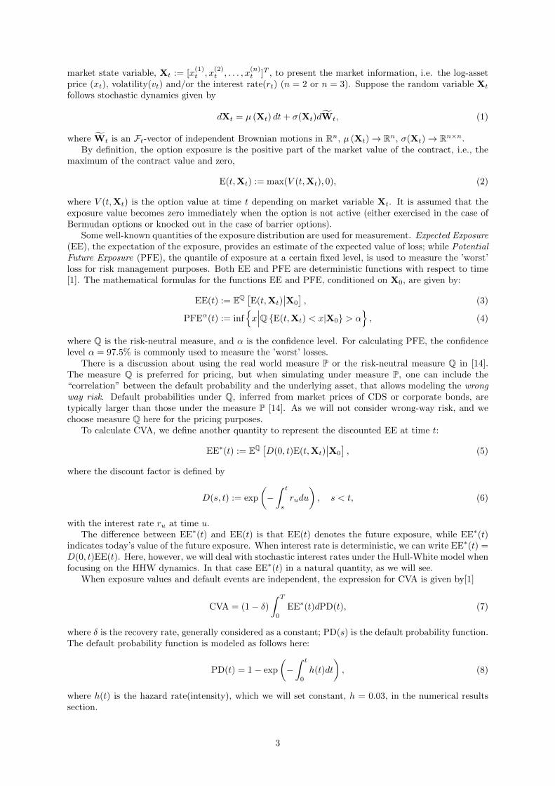
Valuation of Credit Valuation Adjustment (CVA) has become an important field as its calculationis required in Basel III, issued in 2010, in the wake of the credit crisis. Exposure, which is definedas the potential future loss of a default event without any recovery, is one of the key elements forpricing CVA. This paper provides a backward dynamics framework for assessing exposure profiles ofEuropean, Bermudan and barrier options under the Heston and Heston Hull-White asset dynamics.We discuss the potential of an efficient and adaptive Monte Carlo approach, the Stochastic GridBundling Method (SGBM), which employs the techniques of simulation, regression and bundling.Greeks of the exposure profiles can be calculated in the same backward iteration with little extraeffort. Assuming independence between default event and exposure profiles, we give examples ofcalculating exposure, CVA and Greeks for Bermudan and barrier options.

Keywords: Credit Valuation Adjustment (CVA), exposure profiles, European, Bermudan, barrier options,Stochastic Grid Bundling Method, Monte Carlo simulation, least-squares-polynomial-approximation,Greeks, Heston model, Heston Hull-White-model.

1 Introduction

Counterparty Credit Risk (CCR) refers to the risk that a counterparty of a financial contract will defaultprior to the expiration of the contract, and thus cannot make all payments required by the contract.The management of CCR has caught special attention since the financial crisis which started in 2007[1]. OTC (over-the-counter) derivative contracts are especially subject to CCR, since trades are madedirectly between two parties without supervision of a third party. Basel III issued in 2010 introducedan additional capital charge requirement, called Credit Valuation Adjustment (CVA) to cover the riskof losses on a counterparty default event for OTC derivatives. The CVA equals the difference betweenthe risk-free value and the market value of a contract with the possibility of counterparty default, whichindicates that CVA materializes the market value of CCR [1].

One difficulty in pricing CVA arises from the uncertainty of the losses in the event of default, whichis commonly defined as Exposure. As the market moves, exposure values of contracts evolve over time,diverting away from the initial book value [1].

The presence of CCR may have significant impact, for example, on the exercise-strategy of a Bermu-dan option, as the holder can decide to exercise the option earlier to reduce the risk of a future defaultevent [2]. In the present paper however, we assume independence between default and exposure values,and we further assume that the presence of counterparty default has no influence on the holder’s decisionof exercising options.

Monte Carlo simulation is a widely used approach to determine an empirical distribution of theunderlying asset, but also other pricing approaches have been adapted to the computation of exposure.In [3], the COS method is adapted for pricing the exposure of Bermudan options under Levy process ;in [4], the finite difference method is employed for calculation of the exposure values under the Hestonmodel.

∗CWI, center for mathematics and computer science, Amsterdam, the Netherlands, qian@cwi.nl†CWI center of mathematics and computer science, and Delft University of Technology, Delft, the Netherlands,

c.w.oosterlee@cwi.nl

1

arX

iv:1

412.

3623

v1 [

q-fi

n.C

P] 1

1 D

ec 2

014

One focus of this paper is to develop and understand an adaptive and efficient Monte Carlo approach,the Stochastic Grid Bundling Method (SGBM) for computation of exposure profiles of European, Bermu-dan, barrier options with a single asset under stochastic volatility and stochastic interest rate dynamics(Heston and Heston Hull-White model, respectively).

We will study the convergence and performance of SGBM for valuing mainly the exposure of Bermu-dan options, determine accurate Greeks, and also present the corresponding results for barrier options.

SGBM was proposed for pricing Bermudan multiple asset derivative contracts under Black-Scholesdynamics, by Jain and Oosterlee in [5]. The method is based on simulation, regression and bundling.The idea of using simulation and regression for pricing American options has been used earlier byCarriere(1996) [6], Tsitsiklis and Van Roy(2001) [7], or Longstaff and Schwartz(2001) [8]. All thesemethods, though different in some aspects, approximate the continuation value at each time point basedon regression to determine the optimal exercise-strategy. There are several modifications and comparisonsof the original pricing techniques, like in [9], or Broadie, Glasserman and Ha (2000) [10]. In [11],Glasserman and Yu(2002) compare the so-called ’regression later’ approach with a ’regression now’approach, and conclude the superiority of ’regression later’. SGBM is also based on the ’regression laterapproach’; in combination with bundling of grid points at each simulated time step, the regression stepis enhanced. An important feature of SGBM is that at each time point the option value (and thusthe exposure value) is available at each grid point of the stochastic grid, not only for in-the-moneypoints. This is beneficial within the dynamic programming principle giving accurate direct estimators,and facilitates the accurate computation of Greeks at all time points. In section 3, the framework toapply SGBM for computing exposure profiles for European, Bermudan and barrier options is explained;we will give insight in the approximation of the option and continuation values on a polynomial space,and thus on the choice of basis functions for the regression step; based on convergence analysis, the needto use bundles can be explained. Computational details and numerical results for Heston and the HestonHull-White (HHW) models are given in sections 4, respectively.

The HHW model is a useful model when pricing long-term contracts in which we observe an impliedvolatility smile in the asset, and we require a stochastic interest rate. The model is encountered in FXmarkets, for example, as well as in embedded options or inflation options in the pension and insuranceindustry. Our SGBM exposure pricing technique for the HHW model is based on approximations of thefull-scale dynamics in [12].

Before we start to focus on SGBM, we will give an overview of the concepts and mathematicalformulation of CVA and exposure, and provide a backward pricing dynamics of pricing in section 2.

2 CVA, exposure and option pricing

Basically, there are three key elements in pricing CVA: (1) loss given default (LGD), which is thepercentage of loss in a default event, (2) expected exposure (EE), which quantifies the expectation of thelosses at a future time point and (3) probability of the counterparty default (PD). It is often assumedthat LGD is a fixed ratio based on market information, and we also make the assumption that LGD isconstant [1].

In a general real-life situation however these three elements are correlated and not independent, asindicated by the concept wrong-way (or right-way) risk. Here, we assume independence and focus on theaccurate computation of exposure and the corresponding Greeks under stochastic volatility/stochasticinterest rate asset dynamics. The wrong-way risk concept is left for our future research.

Credit exposure represents the economic loss for the derivatives contract holder in a default eventwithout any recovery. The contract holder suffers a loss only if the contract has a positive mark-to-market (MtM) value when the other party defaults, i.e. the exposure is defined as the maximum of thecontract’s market value and zero. We are concerned with unilateral CVA in this paper, although CCRis bilateral between two parties in the contract.

The future exposure value is uncertain as the market moves unpredictably. We can generate an em-pirical exposure density via simulation by generating a large number of asset paths. A general frameworkis presented for calculating exposure distributions on OTC derivative products at each future point in[13]. There are three basic steps in the valuation of exposure profiles: (1) Monte Carlo path generationfor a series of simulation dates under some underlying dynamics; (2) valuation of mark-to-market val-ues of the contract for each realization at each simulation date, applying some numerical method; (3)calculation of exposure for each simulation at each simulation date.

In order to quantify exposure and CVA, we need mathematical expressions. We use an n-dimensional

2

market state variable, Xt := [x(1)t , x

(2)t , . . . , x

(n)t ]T , to present the market information, i.e. the log-asset

price (xt), volatility(vt) and/or the interest rate(rt) (n = 2 or n = 3). Suppose the random variable Xt

follows stochastic dynamics given by

dXt = µ (Xt) dt+ σ(Xt)dWt, (1)

where Wt is an Ft-vector of independent Brownian motions in Rn, µ (Xt)→ Rn, σ(Xt)→ Rn×n.By definition, the option exposure is the positive part of the market value of the contract, i.e., the

maximum of the contract value and zero,

E(t,Xt) := max(V (t,Xt), 0), (2)

where V (t,Xt) is the option value at time t depending on market variable Xt. It is assumed that theexposure value becomes zero immediately when the option is not active (either exercised in the case ofBermudan options or knocked out in the case of barrier options).

Some well-known quantities of the exposure distribution are used for measurement. Expected Exposure(EE), the expectation of the exposure, provides an estimate of the expected value of loss; while PotentialFuture Exposure (PFE), the quantile of exposure at a certain fixed level, is used to measure the ’worst’loss for risk management purposes. Both EE and PFE are deterministic functions with respect to time[1]. The mathematical formulas for the functions EE and PFE, conditioned on X0, are given by:

EE(t) := EQ [E(t,Xt)∣∣X0

], (3)

PFEα(t) := infx∣∣∣Q E(t,Xt) < x|X0 > α

, (4)

where Q is the risk-neutral measure, and α is the confidence level. For calculating PFE, the confidencelevel α = 97.5% is commonly used to measure the ’worst’ losses.

There is a discussion about using the real world measure P or the risk-neutral measure Q in [14].The measure Q is preferred for pricing, but when simulating under measure P, one can include the“correlation” between the default probability and the underlying asset, that allows modeling the wrongway risk. Default probabilities under Q, inferred from market prices of CDS or corporate bonds, aretypically larger than those under the measure P [14]. As we will not consider wrong-way risk, and wechoose measure Q here for the pricing purposes.

To calculate CVA, we define another quantity to represent the discounted EE at time t:

EE∗(t) := EQ [D(0, t)E(t,Xt)∣∣X0

], (5)

where the discount factor is defined by

D(s, t) := exp

(−∫ t

s

rudu

), s < t, (6)

with the interest rate ru at time u.The difference between EE∗(t) and EE(t) is that EE(t) denotes the future exposure, while EE∗(t)

indicates today’s value of the future exposure. When interest rate is deterministic, we can write EE∗(t) =D(0, t)EE(t). Here, however, we will deal with stochastic interest rates under the Hull-White model whenfocusing on the HHW dynamics. In that case EE∗(t) in a natural quantity, as we will see.

When exposure values and default events are independent, the expression for CVA is given by[1]

CVA = (1− δ)∫ T

0

EE∗(t)dPD(t), (7)

where δ is the recovery rate, generally considered as a constant; PD(s) is the default probability function.The default probability function is modeled as follows here:

PD(t) = 1− exp

(−∫ t

0

h(t)dt

), (8)

where h(t) is the hazard rate(intensity), which we will set constant, h = 0.03, in the numerical resultssection.

3

The market value of the contract is observed at a set of discrete times, T =tm∣∣m = 0, 1, . . . ,M

,

with t0 = 0, tM = T , T being the tenor of the contract. The notation of the variables at time tm issimplified by Xm := Xtm . A discrete version of the CVA formula in (7) can be written as

CVA ≈ (1− δ)M−1∑m=0

EE∗(tm) (PD(tm+1)− PD(tm)) . (9)

In (9), the key elements to calculate CVA are the values of the EE∗(t) function and the default prob-ability at the discrete observation dates. We are also interested in values of the PFE function and thecorresponding Greeks. Hence it becomes crucial to validate exposure of each realized scenarios at allsimulated dates.

2.1 Backward pricing dynamics of options

In this section, we present the backward pricing dynamics framework for financial derivatives. When anoption is exercised, the holder receives the payoff value, i.e.

g(Sm) := max (ω(Sm −K), 0) , with

ω = 1, for a call;

ω = −1, for a put,(10)

where Sm = exp(xm) is the underlying asset variable at time tm.When the option contract is still alive, the discounted option value, the continuation value w.r.t.

state vector Xm, reads

cm(Xm) := EQ[Vm+1(Xm+1) ·D(tm, tm+1)

∣∣∣∣Xm

], (11)

where Vm+1(·) represents the option value at time tm+1. At time tM = T , cM := 0. A filtration satisfiesF0 ⊂ · · · Fm ⊂ · · · FM , which describes the information flow.

We establish the backward pricing dynamics framework based on the Snell Envelope concept [15].The owner of the American option makes the exercise decision for the option based on the informationat time tm.

For European options, the option value equals the continuation value before maturity and the holderreceives the payoff value only at time tM , i.e.

V Eurom (Xm) =

g(SM ), for tM ,

cm(Xm), for tm ∈ T − tM .(12)

For Bermudan options, the problem becomes more involved as the option holder has the right toexercise the option at a series of times before maturity. We make the assumption here that the creditinformation of the counterparty does not influence the exercise decision of the option holder: the holdermakes the exercise decision based on the maximum profit he/she can gain. So, at each exercise date theholder compares the payoff value with the continuation value of the option, conditioned on the currentmarket information. Once the payoff value is higher, the option will be exercised; otherwise the holderwill hold the option.

Suppose that the option holder is allowed to exercise the option at the exercise dates, Te =te∣∣te ∈ T , e > 0

.

When the option is still active at time tm, the Bermudan option can be computed via

V Bermm (Xm) =

max cm(Xm), g(Sm) , for tm ∈ Te,cm(Xm), for tm ∈ T − Te.

(13)

We construct the pricing dynamics for barrier options in a similar way. Barrier options becomeactive/knocked out when the underling reaches a predetermined level (the barrier). There are four maintypes of barrier options: up-and-out, down-and-out, up-and-in, down-and-in options. Here we focus ondown-and-out put barrier options.

A down-and-out put barrier option is active initially and gets value zero when the underlying reachesthe barrier; if the option is not knocked out during its lifetime, the holder will receive the payoff value atthe end of the contract. At time tm, when the option is still active, the pricing dynamics are given by,

V barrm (Xm) =

g(Sm) · 1Sm≤L, for tM ,

cm(Xm) · 1Sm≤L, for tm ∈ T − tM ,(14)

4

where 1 (·) is the indicator function.The value of the exposure is defined as the value of the option when the option is still active. When

the option is exercised/knocked out, the exposure value becomes 0. The pricing dynamics of the exposurecan be put in the following formulas:

Em(Xm) =

0, when the option is knocked out;

Vm(Xm), when the option is alive;(15)

where Em(·) represents the exposure at time tm, m = 1, 2, · · · ,M − 1. We define EM = 0.Once options have been exercised/knocked out at time tm, the exposure later than time tm becomes

zero.

3 Stochastic Grid Bundling Method

We present the Stochastic Grid Bundling Method (SGBM). SGBM is based on simulation, bundling andregression. A stochastic grid is defined via generation (simulation) of a large number of stochastic paths,where we can determine the empirical distribution of the state variable at each future time point. Denotethe values of the state variables of the i-th path at time tm as xm(i), i = 1, . . . , N , and once we computedthe exposure values of these scenarios at times tm, m = 0, . . . ,M − 1 the values of the EE function canbe approximated by

EE(tm) ≈ 1

N

N∑i=1

Em(xm(i)), (16)

where N represents the number of paths. The values of the PFE function can also be approximated bythe corresponding quantiles based on the realized exposure values of the generated scenarios.

The exposure profiles presented in formula (16) are values without discount factor. However, forpricing CVA, it is the discounted exposure value that is needed. When the stochastic interest rate isdeterministic, the discounted exposure is the product of the discount factor and EE. When the interestrate is stochastic, we need to discount the realized values of the generated scenarios as follows:

EE∗(tm) ≈ 1

N

N∑i=1

(exp

(m−1∑k=0

rk(i) (tk+1 − tk)

)· Em(xm(i))

), (17)

where rk(i) is the realized interest value at time tk in the i-th path.The option values at the paths at each time point are needed for the calculation of the exposure

distribution, and thus the continuation values, defined in (11), of all paths at each time point need to becalculated. In the following sections, we discuss how to approximate the continuation values in SGBM.

3.1 Least-squares approximation

Option function Vm+1(·) at time tm+1 is L2-measurable on a bounded domain Im+1 , and we approximateit by a simpler function Vm+1(·), i.e.

Vm+1(Xm+1) ≈ Vm+1(Xm+1), Xm+1 ∈ Im+1. (18)

The approximation is made by projecting the option onto a polynomial space, where the values arelinear combinations of H basis functions, defined by

Pp(Im+1) = f |f(x) =

H∑k=1

β(k)ψk(x), x ∈ Im+1,∀k, β(k) ∈ R, (19)

where p is the order of the polynomial subspace, and H represents the number of basis functions. Thus,the approximated option value can be written as

Vm+1(Xm+1) =

H−1∑k=0

β(k)ψk(Xm+1), Xm+1 ∈ Im+1, (20)

5

where the coefficient set β(k)H−1k=0 can be determined in least-squares sense by regression when option

values at time tm+1 are available,

min∀k,β(k)∈R

N∑i=1

(Vm+1(xm+1(i))−

H−1∑k=0

β(k)ψk(xm+1(i))

)2

. (21)

Essentially, formula (21) gives the best approximation on polynomial space Pp(I) of the option func-tion in the L2 norm, which is called the projection on polynomial space Pp(I). Notice that approximatinga function by interpolation and approximating a function in least-squares sense are two different con-cepts. By interpolation, the values of the approximation function are exact at discrete nodes, while whenapproximating in least-squares sense, we study the approximation in average. In the latter case, we findthe projection of the function f onto some subspace Ω, denoted by PΩ, such that the difference f −PΩfis orthogonal to all functions in subspace Ω [16]. The L2 projection does not need to be continuous, orhave well-defined nodal values, which is convenient in our case, as the grid nodes have been generatedvia simulation.

When we approximate the option function by a linear combination of basis functions, the continuationfunction at the earlier time point can be approximated by a linear combination of conditional expectationsof the discounted basis functions, i.e.

cm (Xm) ≈ cm (Xm) = EQ[Vm+1(Xm+1) ·D(tm, tm+1)

∣∣∣∣Xm

]= EQ

[H−1∑k=0

β(k)ψk(Xm+1) ·D(tm, tm+1)

∣∣∣∣Xm

]

=

H−1∑k=0

β(k)EQ[ψk(Xm+1) ·D(tm, tm+1)

∣∣∣∣Xm

]

=

H−1∑k=0

β(k)φk(Xm), (22)

where we denote the conditional expectations of the discounted basis functions by

φk(Xm) := EQ[ψk(Xm+1) ·D(tm, tm+1)

∣∣∣∣Xm

], k = 0, . . . ,H. (23)

In fact, it is easy to see that the span of the series φkkk=0 forms a closed subspace of functions inL2 space, denoted as:

EP(Im) = Ef |Ef(x) =

H∑k=1

β(k)φk(x), x ∈ Im, β(k) ∈ R,∀k. (24)

In other words, we approximate the continuation function on space EP(Im), and the coefficients areobtained via approximation of the option function at a later time point tm+1.

When the basis functions are chosen such that analytic formulas of the corresponding conditionalexpectations of the discounted basis functions are available, the continuation value can be calculatedimmediately, and the option value at the same point can be calculated applying formulas (12), (13) and(14) for European, Bermudan or barrier options, respectively.

Though there are many possibilities for choosing the set of basis functions for a polynomial space oforder p, we choose monomials of degree equal or lower than order p as the basis functions. A monomialis a polynomial with only one term, which can be defined as a product of powers of variables withnon-negative integer exponents. The degree of a monomial is defined as the sum of all exponents of thevariables. Considering an n-dimensional problem with a polynomial space of order p, it is easy to seethat the set of monomials with degree less or equal to order p is a span of polynomials1, and the total

number of these basis functions is equal to 1(n−1)!

∑pd=0

(d+n−1)!d! .

It is convenient to construct the polynomial subspace with monomials. Moreover, we then haveanalytic formulas for the expectations of the discounted monomials: when we use monomials as the basisfunctions, the conditional expectations of the discounted basis functions are discounted moments. For2-d dynamics these moment are given in definition 3.1.

1The number of monomials of n variable with order d is(d+n−1)!(n−1)!d!

.

6

Definition 3.1 (Discounted moments) In a time period [t, T ], t < T , conditioned on the informa-tion at time t, the discounted moments of a state variable Yt = [yt, zt]

T of order p + q is defined asEQ [(yT )

p · (zT )q ·D(t, T )

∣∣Yt

].

There is a useful link between the discounted moments and the discounted characteristic function(dChF) of the dynamics. By derivatives w.r.t yT and zT , respectively, we find

EQ [(yt)p · (zt)q ·D(t, T )∣∣Yt

]=

1

(i)p+q· ∂

pΦ

∂up1· ∂

qΦ

∂uq2(u1, u2; Yt, t, T )

∣∣∣∣u1=0,u2=0

, (25)

where Φ(; ) is the dChF. The higher-dimensional case can be defined in a similar way.For the constant basis function (of degree 0), the discounted first moment equals the zero coupon

bond in interval [t, T ]:

φ0(Xt) = φ0 := EQ [D(t, T )|Xt] = EQ[e−

∫ Ttrudu

∣∣Xt

]=: P (t, T ). (26)

Once analytic formulas of the discounted moments are derived, multiplication of the coefficient setsdetermined at time tm+1 gives us the formula for approximating the continuation value at time tm.

3.2 Greeks

The state variable Xm must at least contain the underlying asset information, and we always put thelog-asset variable as the first element in the vector that Xm = [xm, . . . ]

T , where xm := log(Sm). Herewe present the sensitivity w.r.t the initial asset value S0, which can be applied for all models discussedin this paper.

It is direct to approximate the sensitivities of the exposure profile in SGBM. At time tm, the sensitivityDelta (∆) of the EE w.r.t the change in the underlying asset price S0 can be derived by

∆EE(tm) =∂EE(tm)

∂S0≈ 1

N

N∑i=1

∂Em∂S0

(xm(i))

=1

N

N∑i=1

∂Em∂xm

· ∂xm∂Sm

· ∂Sm∂S0

(xm(i)) , m = 0, . . . ,M − 1, (27)

where xm(i) = [log(Sm(i)), . . . ]T is the i-th realization at time tm of the state variable; applying thechain rule and calculating the partial derivative, we get2

∂xm∂Sm

=1

Sm,

∂Sm∂S0

=SmS0

, m = 0, . . . ,M − 1. (30)

The first-derivative of the exposure profile is defined as:

∂Em∂xm

:=

0 when the option is exercised,∂cm∂xm

when the option is active,m = 0, . . . ,M − 1, (31)

with formula (22), the first derivative of the continuation function w.r.t Xm is approximated by

∂cm∂Xm

≈ ∂cm∂Xm

=

H∑k=0

β(k)∂φk∂Xm

, m = 0, . . . ,M − 1, (32)

2 Since

Sm = S0 exp

((rm −

1

2σ2m

)tm + σmW

xtm

), (28)

it is easy to derive that:

∂Sm

∂S0= exp

((rm −

1

2σ2m

)tm + σmW

xtm

)=Sm

S0, (29)

where σm =√vm and rm, are the volatility and interest rate at time tm respectively. Here the variance variable and

interest rate can be either a constant or a stochastic value.

7

where the coefficient set is the same as in (22). Hence

∆EE(tm) ≈ 1

N

N∑i=1

∂Em∂xm

(xm(i)) · 1

S0, m = 0, . . . ,M − 1, (33)

Further, we can get an easy formula for Gamma (Γ), as

ΓEE(tm) ≈ 1

N

N∑i=1

(∂2Em∂X2

m

(xm(i))− ∂Em∂xm

(xm(i))

)· 1

S20

, m = 0, . . . ,M − 1, (34)

Comment: In a similar way, we are able to calculate Rho(ρ), which is defined as the sensitivity tothe interest rate r0, and Vega(ν), which is the sensitive to the volatility v0. However, it is a somewhatinvolved to calculate Vega(ν) along the whole time horizon as it is nontrivial to calculate ∂vm

∂v0.

3.3 Convergence and choice of bundles

There are interesting studies on the convergence and bias of Monte Carlo based regression methods. In[17], Clement, Lamberton and Protter prove the almost surely convergence of the Longstaff-Schwartzalgorithm and determine the rate of the convergence. Other available studies show that there is anupward-bias in the direct estimates, and the result based on the obtained optimal exercise-strategy isa lower bound estimate of the option price [8, 7, 9]. In [18], Broadie and Cao propose to apply a localsimulation to improve the lower and upper bound algorithms and reduce the variance.

When approximating the option value, there are two types of errors appearing [17]:

• Type 1 : the error source is the difference between the true and the approximate option values, asthe value is approximated by its projection onto a polynomial space. This error is related to theproperties of the polynomial space;

• Type 2: the error source is the noise in estimating the coefficients via regression based on sampleddata, which related to the accuracy of the Monte Carlo simulation and thus to the number of paths.

We need to reduce the errors of Type 1 and Type 2. According to Central Limit Theorem, the errorof Type 2 can be diminished by increasing the number of paths to infinity with probability 1 a.s. [17].Some available results show that the error of Type 1 goes to zero when the number of basis functionsgoes to infinity as well [5]. In this paper, we will present an accurate upper bound for the error of Type1 related to the properties of the polynomial space, and give a reasoning for the use of bundles.

In [17], the discussion is on the error of Type 2. Although it is focused on the Longstaff-Schwartzmethod, the analysis can be applied to our method as well. As in [17], we add the error of Type 2 as anoise term:

V (Xm+1) = V (Xm+1) + εm+1, (35)

V (Xm+1) =

H∑k=0

β(k)ψk(Xm+1), (36)

where when the number of paths N is sufficiently large, εm+1 ∼ N (0,σ2m+1

N ) i.i.d, and independent of

variable Xm+1 ; V (·) is the ’true’ value of the option on the polynomial space, whereas V (·) is theapproximation of the option with the coefficients set β(k)Hk=1.

We futher define the approximation of the continuation function as:

cm(Xm) := EQ[Vm+1(Xm+1) ·D(tm, tm+1)

∣∣∣∣Xm

], (37)

hence

cm(Xm) ≈ cm(Xm) = cm(Xm) + εm+1, (38)

We first give a proposition regarding the boundedness of the error of the approximating continuationvalue by the error of the approximating option value in the L2 norm.

8

Proposition 1 Assuming that ∀Xm ∈ Im, the conditional density function satisfies∫Im+1

f(Xm+1;Xm)dXm+1 = 1− ε, Xm+1 ∈ Im+1, (39)

where f(·;Xm) is the density function conditioned on Xm, ε is a small error generated by the truncationof the integration range. The error of approximating the continuation function at time tm can be boundedby the error of approximating the option function at time tm+1 as:

‖cm − cm‖L2(Im) ≤ ‖Vm+1 − Vm+1‖L2(Im+1) ·√

(1− ε)h(Im), (40)

where h(Im) is the size of the bounded domain Im.

Proof is given in Appendix A.1.Proposition 1 ensures that, when the approximation of the option function is accurate, the approx-

imation of the continuation function at an earlier stage will be accurate as well. The boundedness inProposition 1 includes errors of both Type 1 and Type 2.

For Error of Type 1, we give two well-known insights, from [16] and [19] , which gives a bound of theerror by projection onto a linear polynomial space in a 1-d and 2-d domain, respectively.

Theorem 3.2 In a one-dimensional domain I, suppose that the function f(x) is twice differentiable,and P1(I) is the linear polynomial space. The projection onto the space P1(I) in interval I in the L2

norm satisfies the best approximation result,

minf∈P1(I)

‖f − f‖L2(I) ≤ Ch2‖f (2)‖L2(I), (41)

where h is the length of the interval I and f (2) is the second derivative function.

Theorem 3.3 In a two-dimensional domain I, suppose that the function f(x1, x2) is twice differentiable,and P1(I) is the linear polynomial space. The projection onto the space P1(I) in interval I in the L2

norm satisfies the best approximation result

minf∈P1(I)

‖f − f‖L2(I) ≤ Ch2‖D2f‖L2(I), (42)

where h is a representative size of the mesh and D2 is a 2-d differential operator with mixed derivatives.

The details of the construction of the mesh can be found in [19].Theorems 3.2 and 3.3 provide upper bounds of the error by approximating a function by its projection

on a linear polynomial space. Though we do not know much about the properties of the function, theerror can be reduced by approximating the function on some discrete subdomains I1, . . . , IJ , such thatI = ∪Ji=1I

i, the projection of the function in each subdomain Ii is written as

f(x) ≈ fi(x), x ∈ Ii, , i = 1, . . . , J. (43)

In 1-d notation, the error can be bounded by,

J∑i=1

minfi∈P1(Ii)

‖f − fi‖L2(Ii) ≤ CJ∑i=1

h2i ‖f

(2)i ‖L2(Ii) ≤ C

(J

maxi=1

hi

)2

‖f (2)‖L2(I), (44)

where Ii is the size of Ii.It tells us that the error can be reduced efficiently by approximating the function in subdomains.

Theorems 3.2 and 3.3 give upper bounds for projection on a linear polynomial space (p = 1). Wegeneralize the results to a polynomial space of order p, in Proposition 2.

Proposition 2 In a 1-d interval I, suppose that the function f(x) is (p + 1) times differentiable, andPp(I) is a polynomial of order p on I. The projection on the space Pp(I) on interval I in the L2 normsatisfies the best approximation result as follows

minf∈Pp(I)

‖f − f‖L2(I) ≤ Chp+1‖f (p+1)‖L2(I), (45)

where h is the length of interval I.

9

Proof is given in Appendix A.2.Proposition 2 provides a rough estimate of the accuracy of the approximation function in the poly-

nomial subspace Pp(I) for a 1-d problem. The accuracy depends on the length of the interval, thepolynomial order and the value of the (p+ 1)-th derivative.

In practice, the determination of subdomains is done in SGBM by making bundles from the simulatedpaths. We define the subdomains at time tm+1 by clustering paths into bundles at time tm. One aim isto satisfy the assumptions in Proposition 1. The paths at time tm are clustered based on criteria, so thatthe values of paths in the same bundle fall into the same subdomain at time tm+1. When all subdomainsare of the same size, the 1-d accuracy can be approximated by

J∑i=1

minV jm+1∈Pp(Iim+1)

‖Vm+1 − V jm+1‖L2(Iim+1) ∼C2

J (p+1)‖f (p+1)‖L2(Im+1), (46)

where J is the number of bundles.V jm+1 is the exact projection of the function on the polynomial space within the j-th bundle. In

practice, we estimate it by regression, denoted by V jm+1, based on cross-sectional data, where the errorof Type 2 plays its role. We need to ensure that there are enough paths within each bundle, so that theerror of Type 2 is sufficiently small, otherwise it is meaningless to analyze the error of Type 1.

We propose a principle for defining the bundles: cohesive in value and equal in number. In short,within each bundle, the state variable path values should be as close as possible, and the paths shouldbe distributed into each bundle in a way such that there are ’sufficient’ paths within each bundle. Insection 4, methods of making bundles are presented.

3.4 Backward iteration for exposure values

We present the procedure for calculating the exposure values in a backward iteration, starting at finaltime T . Suppose the path generation has finished and the realized values of the state variable of Npaths at all observation dates tmMm=0 are available, denoted by xm(i),m = 0, . . . ,M, i = 1, . . . , N.At time tM , the exposure values are set to 0 as the contract ended. The option value of the i-th path iscalculated as VM (xM (i)), for European, Bermudan or barrier options, applying formulas (12), (13) and(14), respectively.

At time tM−1, the paths are clustered into J bundles applying some bundling method, and we denotethe j-th bundle at time tM−1 by BM−1,j . On a polynomial space of order p, where there are H basisfunctions in the span, we can find the ’best coefficients set’ via OLS regression within the same bundleby minimizing the following expression,

min∀β(k,BM−1,j)∈R

∑paths in bundle BM−1,j

(VM (xM (i))−

H∑k=0

β(k,BM−1,j)ψk(xM (i))

)2

, (47)

where the k-th coefficient at time tM−1 in the j-th bundle is denoted by β(k,BM−1,j), and thus at timetM , within the j-th bundle, the option function can be approximated by

VM (XM ) ≈H−1∑k=0

β(k,BM−1,j)ψk(XM ), for values of paths in bundle BM−1,j , (48)

With (22), the analytic formula of the approximation of the continuation function at time tM−1,

cM−1(XM−1) ≈H−1∑k=0

β(k,BM−1,j)φk(XM−1), for values of paths in bundle BM−1,j at tM−1, (49)

where φk(·) defined in (23) represents the corresponding discounted moments.Hence for all paths, the continuation values cM−1(xM−1(i)), i = 1, . . . , N , can be calculated directly;

the option values at the i-th path at time M − 1, VM−1(xM (i)), and the exposure values, EM−1(xM (i)),can be determined as well.

Then the iteration goes back with one time step to time tM−2, repeating the procedures of bundlingand regression for the calculation of the continuation, option and exposure values. We progress inbackward direction until we reach initial time t0 where we have the option/exposure values of all paths

10

along the whole time horizon. The calculation of the sensitivity values can be done at the same time inthe iteration as it requires the same set of coefficients.

The backward calculation procedure is basically the same for European, Bermudan or barrier op-tions, except that the pricing formulas for option values differ: we apply formulas (12), (13) and (14),respectively, for these options.

When computing exposure profiles for Bermudan options, we also need to determine the optimal early-exercise strategy. At time tm, if the option has not been exercised, both option and exposure values ateach path are set to the corresponding continuation value; for each path, the payoff value is calculated, andcompared with the continuation value to determine whether the option should be exercised, conditionedon the available information. For a specified path, if the option should be exercised, the exposure at thispath from time tm on will be equal to zero, and the option value at time tm is equal to the payoff value.

We store the ”optimal“ exercise strategy for all paths and the corresponding cash flow, and estimatethe corresponding EE value at a time point by taking the mean of the discounted cash-flow as:

EE(tm) ≈ 1

N

∑τi>tm

(D(tm, τi) · cash-flow(i)) , (50)

where τi is the exercise time (or stopping time) of the i-th path, and the cash flow is the payoff value attime τi, known as

cash-flow(i) :=g(Sτi(i)) = max (ω(Sτi(i)−K), 0) , with

ω = 1, for a call;

ω = −1, for a put,(51)

with Sτi(i) the value of the stock of the i-th path at time τi. If the option is not exercised for somepaths and expiration dates, then the cash flow value is just zero. Notice that the discount factor needsto be incorporated in the realized values along each simulated path when dealing with stochastic interestrates.

In practice, we call the EE values calculated via formula (16) the direct estimators. and EE valuescalculated via formula (50) based another set of simulated scenarios the path estimators. The detailedprocedure calculating the path estimator is as follows:

• In the regression procedure of in the backward iteration, at each time point, the coefficient sets ofeach bundle are saved;

• We simulate another set of paths of twice the size;

• We calculate backward from time tM−1 till time t0:

– at time tm, make bundles, and use the same coefficient set of each bundle obtained in the firstsimulation to determine the continuation values of the paths;

– calculate the option value and determine the exercise strategy at each path at time tm; savethe exercise strategy of each path and the corresponding cash flow values;

• Applying formula (50) to calculate the EE values based on the obtained ”optimal” exercise strategy.

3.5 Comments

The path estimator is commonly the lower bound while the direct estimator represents the upper bound[8, 5], because of the convexity property of the “max“ function. This is a useful result and we can testthe convergence of SGBM by comparing the difference between these upper and lower bounds.

For Bermudan options, the estimation of the exposure heavily depends on the accuracy of the ”op-timal” early-exercise strategy. There is a discontinuity in the exposure function at the early-exercisepoint, thus at the exercise date, the exposure value jumps immediately to zero for a specific path whenthe option is exercised; if the calculated “optimal“ early-exercise strategy is inaccurate, the differencebetween the ’true’ and the calculated exposure values would be as high as the option value at this timepoint. Pricing an option at each time point is much less sensitive to the accuracy of the ”optimal“early-exercise strategy as the option function is smooth.

11

4 Basis functions and bundles

As we see, the number of basis functions is equal to (n+p)!n!p! , where n is the dimension and p is the order

of the polynomial space. We will apply bundling to enhance the accuracy.

4.1 Heston model

We consider the 2-d state variable Xt = [xt, vt]T , with xt = log(St) the log-asset variable and vt represents

the variance variable. The dynamics are given by the Heston stochastic volatility model

dvt = κ(v − vt)dt+ γ√vtdW

vt ,

dxt =

(r − 1

2vt

)dt+

√vtdW

xt , (52)

where r is the constant interest rate; W xt and W v

t are Brownian motions, and dW xt · dW r

t = ρx,rdt; theconstant parameters κ, v represent the speed and the mean level of the reverting in the volatility process,and γ is called the vol-of-vol parameter.

The option function is a function of the log-asset price and variance. For orders p = 0, 1, 2, 3, theset of basis functions is presented in table 1.

order p of the polynomial space the corresponding basis functions

0 11 1, x, v2 1, x, v, x2, x · v, v23 1, x, v, x2, x · v, v2, x3, x2 · v, x · v2, v3

Table 1: The basis functions and order p.

The Heston model belongs to the so-called class of affine asset dynamics, which means that analyticformulas for the discounted moments can be obtained, for example, via the dChF. The discountedmoments are given in Appendix B.1.1.

In [5], the recursive bifurcation method was proposed for bundling asset paths when pricing multipleassets under the Black-Scholes model. A reduced space-recursive bifurcation method based on the valuesof the payoff was introduced to reduce the complexity. An important different for bundling under theHeston model is that here the log-asset and variance processes are highly correlated when there is astrong correlation between the Brownian motions of these two processes.

With a large correlation parameter, applying the 2-d recursive bifurcation method directly results inthe problematic fact that we may not have accurate results, as the number of paths in some bundles isnot large enough for accurate regression, not even with a large total number of paths.

Hence we adapt the recursive-bifurcation method by adding a rotation step, and propose anothermethod for bundling as well.

4.1.1 Recursive-bifurcation-with-rotation

The bundles are made based on the cross-sectional data at each time point, and we denote the tworealized data sets at time tm as: d1 = xm(i)Ni=1, and d2 = vm(i)Ni=1. The basic idea is that weproject the correlated data sets d1 and d2 onto two almost independent data sets q1 and q2 by a rotationwith an angle α1.

Step 1: The values of trigonometric functions of the rotation angle α1 are defined as:

cosα1 =

√1

1 + k21

sign(k1), sinα1 =

√k2

1

1 + k21

, (53)

12

where k1 is the slope defined as3

k1 :=E [(xm − E[xm]) (vm − E[vm])]

E[(xm − E [xm])

2] ≈ covariance(d1, d2)

variance(d1)(54)

The new two sets of data are calculated by(q1

q2

)=

(cosα1 sinα1

− sinα1 cosα1

)(d1

d2

)(55)

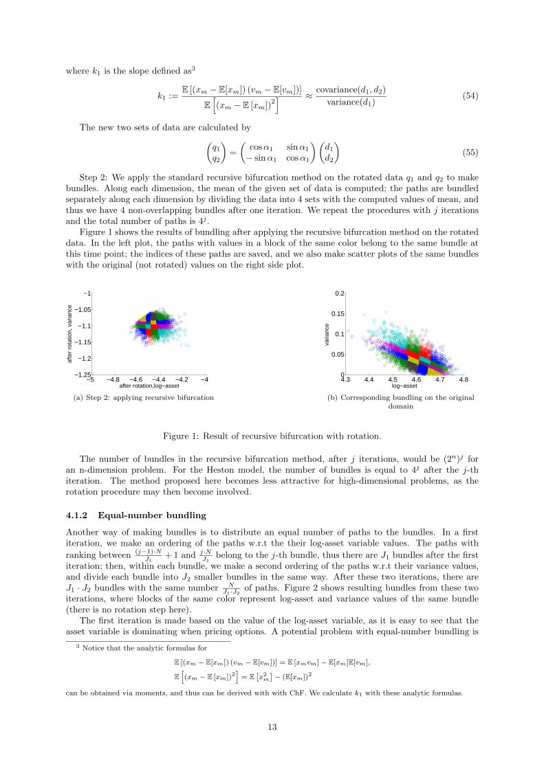
Step 2: We apply the standard recursive bifurcation method on the rotated data q1 and q2 to makebundles. Along each dimension, the mean of the given set of data is computed; the paths are bundledseparately along each dimension by dividing the data into 4 sets with the computed values of mean, andthus we have 4 non-overlapping bundles after one iteration. We repeat the procedures with j iterationsand the total number of paths is 4j .

Figure 1 shows the results of bundling after applying the recursive bifurcation method on the rotateddata. In the left plot, the paths with values in a block of the same color belong to the same bundle atthis time point; the indices of these paths are saved, and we also make scatter plots of the same bundleswith the original (not rotated) values on the right side plot.

−5 −4.8 −4.6 −4.4 −4.2 −4−1.25

−1.2

−1.15

−1.1

−1.05

−1

after rotation,log−asset

afte

r ro

tatio

n, v

aria

nce

(a) Step 2: applying recursive bifurcation

4.3 4.4 4.5 4.6 4.7 4.80

0.05

0.1

0.15

0.2

log−asset

varia

nce

(b) Corresponding bundling on the originaldomain

Figure 1: Result of recursive bifurcation with rotation.

The number of bundles in the recursive bifurcation method, after j iterations, would be (2n)j foran n-dimension problem. For the Heston model, the number of bundles is equal to 4j after the j-thiteration. The method proposed here becomes less attractive for high-dimensional problems, as therotation procedure may then become involved.

4.1.2 Equal-number bundling

Another way of making bundles is to distribute an equal number of paths to the bundles. In a firstiteration, we make an ordering of the paths w.r.t the their log-asset variable values. The paths with

ranking between (j−1)·NJ1

+ 1 and j·NJ1

belong to the j-th bundle, thus there are J1 bundles after the firstiteration; then, within each bundle, we make a second ordering of the paths w.r.t their variance values,and divide each bundle into J2 smaller bundles in the same way. After these two iterations, there areJ1 · J2 bundles with the same number N

J1·J2 of paths. Figure 2 shows resulting bundles from these twoiterations, where blocks of the same color represent log-asset and variance values of the same bundle(there is no rotation step here).

The first iteration is made based on the value of the log-asset variable, as it is easy to see that theasset variable is dominating when pricing options. A potential problem with equal-number bundling is

3 Notice that the analytic formulas for

E [(xm − E[xm]) (vm − E[vm])] = E [xmvm]− E[xm]E[vm],

E[(xm − E [xm])2

]= E

[x2m]− (E[xm])2

can be obtained via moments, and thus can be derived with with ChF. We calculate k1 with these analytic formulas.

13

4.3 4.4 4.5 4.6 4.7 4.80

0.05

0.1

0.15

0.2

log−asset

varia

nce

(a) Step 1: bundles on the log-asset domain

4.3 4.4 4.5 4.6 4.7 4.80

0.05

0.1

0.15

0.2

log−asset

varia

nce

(b) Step 2: bundles on the variance domain

Figure 2: Result of equal-number bundling.

that when the Feller condition is not satisfied, there are zero variance values which may be confusingwhen ordering these paths.

An advantage of equal-number bundling is that one can freely choose the number of subdivisions ineach dimension. We can choose a larger number in log-asset domain, as the log-asset value will have amore significant impact on option values. Equal-number bundling is also more efficient compared to therecursive bifurcation method.

4.2 Heston-Hull-White model

When we add interest rate as a stochastic variable, the state variable becomes Xt := [xt, vt, rt], for whichthe corresponding dynamics are given, under the Heston Hull-White model, by

drt = λ(θ − rt)dt+ ηdW rt ,

dvt = κ(v − vt)dt+ γ√vtdW

vt ,

dxt =

(rt −

1

2vt

)dt+

√vtdW

xt , (56)

with W rt Brownian motion, dW v

t · dW rt = 0 and dW x

t · dW rt = ρx,r; constant parameters λ, θ and η

represent the speed of mean reversion, mean level of the interest rate and the volatility of the interestrate process, respectively; the other parameters are the same as in (52).

Basis functions of the polynomial space of order p, up to order 2, are presented in Table 2.

order p the basis functions

0 11 1, x, v, r2 1, x, x2, v, v2, r, r2, x · v, x · r, r · v

Table 2: The basis functions and order p.

A difficulty when applying SGBM for the HHW dynamics, is that analytic formulas of the discountedmoments are not available as the HHW model does not belong to the affine class when ρx,r 6= 0. We cansee this from the covariance matrix

σ (Xt)σ (Xt)T

=

vt ρx,vvt√vtηρx,r

∗ γ2vt 0∗ ∗ η2

. (57)

Therefore, we will use an affine H1HW model, as proposed in [12], to approximate the HHW modeland to find analytic formulas of the discounted moments for an approximate HHW model.

4.2.1 Basis functions and H1HW model

To obtain an alternative affine formulation of the HHW dynamics, we approximate the stochastic term√v(t) in (57) by a deterministic function, E

[√vt∣∣vs] , which is the conditional expectation of

√v(t) in

14

time interval [s, t], and hence the covariance matrix of the approximate model can be written as:

σ(Xt

)σ(Xt

)T=

vt ρx,vvt E[√vt∣∣vs] ηρx,r

∗ γ2vt 0∗ ∗ η2

. (58)

The model connected to the covariance matrix in (58) is called the H1HW model [12]. Error analysis,comparing the full-scale HHW model with the performance of the approximate H1HW model is givenin [12], where it is shown that the errors in option values is typically very small.

In Appendix B.3, the discounted ChF of the H1HW model is presented, based on which we candetermine the discounted moments.

The expression for the conditional expectation of the volatility is given by:

E[√vt∣∣vs] =

√2c(τ)e−

λ(τ)2

∞∑k=0

1

k!

(λ(τ, vs)

2

)k Γ(

1+d2 + k

)Γ(d2 + k

) , (59)

with τ := t− s,where

c(τ) =1

4κγ2(1− e−κτ ), d =

4κv

γ2, λ(τ, vs) =

4κvse−κτ

γ2(1− e−κτ ), (60)

which is truncated when computing this sum. In numerical calculations, however, it turns out that theformula (59) is not robust, particularly not when τ is small. Hence for small values of τ , the conditionalexpectation of the square root of the variance is approximated as

E[√vt∣∣vs] ≈ √vs,

which is becauseE[√vt∣∣vs]→ √vs, when (t− s)→ 0.

When d > 12 , we can simplify the expression for the conditional expectation of the variance using the

following the formula :

E[√vt∣∣vs] ≈

√c(τ)

(λ(τ, vs)− 1 + d+

d

2(d+ λ(τ, vs))

), (61)

where c(τ), d and λ(τ, vs) are as defined in (59), see [12]. When d < 12 , it is suggested to use the accurate

formula in (59).

4.2.2 Bundles

We develop the two bundling methods in this 3-d problem. First, we present the recursive-bifurcation-with-rotation method for HHW model.

Step 1: project the two sets of data (d1, d2, d3) into two independent sets of data (q1, q2, q3) by thefollowing way. We define the rotation angles α1, α2 as

cosα1 =

√1

1 + β21

sign(β1), sinα1 =

√β2

1

1 + β21

, (62)

cosα2 =

√1

1 + β22

sign(β2), sinα2 =

√β2

2

1 + β22

, (63)

where4

β1 :=E [(xm − E(xm)) (vm − E(vm))]

E[(xm − E[xm])

2] ≈ covariance(d1, d2)

variance(d1), (64)

β2 :=E [(xm − E(xm)) (rm − E(rm))]

E[(xm − E[xm])

2] ≈ covariance(d1, d3)

variance(d1), (65)

4These needed moments can be derived from the (non-discounted) ChF, and we calculate the slopes with the analyticformulas.

15

We rotate data d1, d2 and d3 by angles α1, α2 using the following matrix,q1

q2

q3

=

cosα1 sinα2 sinα1 − cosα1 cosα2

− sinα1 sinα2 cosα1 sinα1 cosα2

cosα2 0 sinα2

d1

d2

d3

(66)

The idea of making bundles in the 3-d case with equal-numbering is also similar as for the Hestonmodel. First, we make a ranking of the paths by their stock values, and determine J1 bundles; after thisiteration, within each bundle, a ranking of the paths is made by the interest rate values to determine J2

bundles in this direction followed by the ranking of the variance values to have J3 sub-bundles withineach bundle. After these three iterations, we have (J1 · J2 · J3) bundles.

Notice that when the Feller condition is not satisfied, there are many ”zeros“ in the variance values ofthe paths. The second bundling step is therefore made with interest rate values. The first step, however,should be based on the stock values, as the option values are dominated by stock values.

4.3 Bundles for barrier options

When we make bundles for pricing barrier options, we only consider the ’active paths’. Hence, we findthe paths that did not reach the barrier, and apply a regular bundling method. This is visualized inFigure 3 as a 2-D example.

4.3 4.4 4.5 4.6 4.7 4.80

0.05

0.1

0.15

0.2

log−asset value

varia

nce

valu

e

(a) recursive-bifurcation-with-rotation,barrier

4.3 4.4 4.5 4.6 4.7 4.80

0.05

0.1

0.15

0.2

log−asset value

varia

nce

valu

e

(b) Equal-number-bundling, barrier

Figure 3: Bundling result for barrier options.

5 Numerical results

In this section, several numerical results obtained by the SGBM method are presented. We first discussthe impact of stochastic volatility and stochastic interest rate on the exposure quantities. Following this,we analyze the convergence and accuracy of SGBM, by comparing the path and direct estimators andby comparing with reference value (obtained via the COS method or the discounted cash flow of thesimulated path).

For all tests presented here, we will employ the Quadratic Exponential (QE) scheme [20] for gen-eration of the forward MC paths, for robustness reasons. We have compared the QE scheme valuationresults with the results obtained with an SDE Euler scheme and concluded that particularly in the casein which the Feller condition is not satisfied the QE scheme is superior.

We have tested several parameter sets for which the Feller condition is satisfied and for which theFeller condition is not satisfied. We found that the Feller condition had very little impact on theperformance of SGBM, due to the method components chosen (QE scheme, type of bundling and choiceof basis functions). We therefore only show results for parameter sets for which the Feller condition isnot satisfied, as it is supposed to be more difficult for valuation. Generally the cases in which the Fellercondition was satisfied were somewhat easier regarding the choice of time step.

We apply formula (9) to calculate CVA with recovery rate δ = 0. The default probability functionhas been defined in equation (8) with a constant intensity h = 0.03.

16

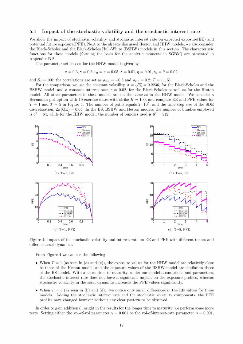
5.1 Impact of the stochastic volatility and the stochastic interest rate

We show the impact of stochastic volatility and stochastic interest rate on expected exposure(EE) andpotential future exposure(PFE). Next to the already discussed Heston and HHW models, we also considerthe Black-Scholes and the Black-Scholes Hull-White (BSHW) models in this section. The characteristicfunctions for these models (forming the basis for the analytic moments in SGBM) are presented inAppendix B.2.

The parameter set chosen for the HHW model is given by

κ = 0.3, γ = 0.6, v0 = v = 0.05, λ = 0.01, η = 0.01, r0 = θ = 0.02,

and S0 = 100; the correlations are set as ρx,v = −0.3 and ρx,r = 0.2; T = 1, 5.For the comparison, we use the constant volatility, σ =

√v0 = 0.2236, for the Black-Scholes and the

BSHW model, and a constant interest rate, r = 0.02, for the Black-Scholes as well as for the Hestonmodel. All other parameters in these models are set the same as in the HHW model. We consider aBermudan put option with 10 exercise dates with strike K = 100, and compare EE and PFE values forT = 1 and T = 5 in Figure 4. The number of paths equals 2 · 105, and the time step size of the SDEdiscretization, ∆t(QE) = 0.05. In the BS, BSHW and Heston models, the number of bundles employedis 43 = 64, while for the HHW model, the number of bundles used is 83 = 512.

0 0.2 0.4 0.6 0.8 10

2

4

6

8

10

time

EE

BS

Heston

BSHW

HHW

(a) T=1, EE

0 1 2 3 4 50

5

10

15

20

time

EE

BS

Heston

BSHW

HHW

(b) T=5, EE

0 0.2 0.4 0.6 0.8 10

10

20

30

time

PF

E

BS

Heston

BSHW

HHW

(c) T=1, PFE

0 1 2 3 4 50

20

40

60

time

PF

E

BS

Heston

BSHW

HHW

(d) T=5, PFE

Figure 4: Impact of the stochastic volatility and interest rate on EE and PFE with different tenors anddifferent asset dynamics.

From Figure 4 we can see the following:

• When T = 1 (as seen in (a) and (c)), the exposure values for the HHW model are relatively closeto those of the Heston model, and the exposure values of the BSHW model are similar to thoseof the BS model. With a short time to maturity, under our model assumptions and parameters,the stochastic interest rate does not have a significant impact on the exposure profiles, whereasstochastic volatility in the asset dynamics increases the PFE values significantly.

• When T = 5 (as seen in (b) and (d)), we notice only small differences in the EE values for thesemodels. Adding the stochastic interest rate and the stochastic volatility components, the PFEprofiles have changed however without any clear pattern to be observed.

In order to gain additional insight in the results for the longer time to maturity, we perform some moretests. Setting either the vol-of-vol parameter γ = 0.001 or the vol-of-interest-rate parameter η = 0.001,

17

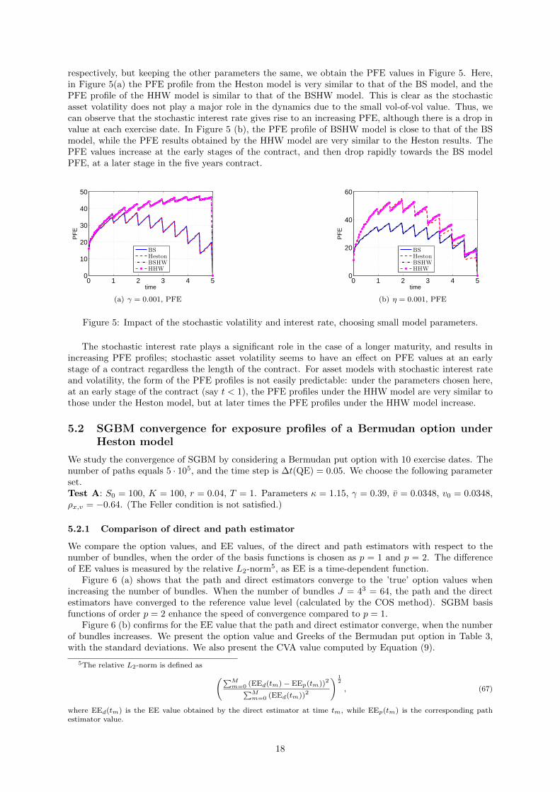
respectively, but keeping the other parameters the same, we obtain the PFE values in Figure 5. Here,in Figure 5(a) the PFE profile from the Heston model is very similar to that of the BS model, and thePFE profile of the HHW model is similar to that of the BSHW model. This is clear as the stochasticasset volatility does not play a major role in the dynamics due to the small vol-of-vol value. Thus, wecan observe that the stochastic interest rate gives rise to an increasing PFE, although there is a drop invalue at each exercise date. In Figure 5 (b), the PFE profile of BSHW model is close to that of the BSmodel, while the PFE results obtained by the HHW model are very similar to the Heston results. ThePFE values increase at the early stages of the contract, and then drop rapidly towards the BS modelPFE, at a later stage in the five years contract.

0 1 2 3 4 50

10

20

30

40

50

time

PF

E

BS

Heston

BSHW

HHW

(a) γ = 0.001, PFE

0 1 2 3 4 50

20

40

60

time

PF

E

BS

Heston

BSHW

HHW

(b) η = 0.001, PFE

Figure 5: Impact of the stochastic volatility and interest rate, choosing small model parameters.

The stochastic interest rate plays a significant role in the case of a longer maturity, and results inincreasing PFE profiles; stochastic asset volatility seems to have an effect on PFE values at an earlystage of a contract regardless the length of the contract. For asset models with stochastic interest rateand volatility, the form of the PFE profiles is not easily predictable: under the parameters chosen here,at an early stage of the contract (say t < 1), the PFE profiles under the HHW model are very similar tothose under the Heston model, but at later times the PFE profiles under the HHW model increase.

5.2 SGBM convergence for exposure profiles of a Bermudan option underHeston model

We study the convergence of SGBM by considering a Bermudan put option with 10 exercise dates. Thenumber of paths equals 5 · 105, and the time step is ∆t(QE) = 0.05. We choose the following parameterset.Test A: S0 = 100, K = 100, r = 0.04, T = 1. Parameters κ = 1.15, γ = 0.39, v = 0.0348, v0 = 0.0348,ρx,v = −0.64. (The Feller condition is not satisfied.)

5.2.1 Comparison of direct and path estimator

We compare the option values, and EE values, of the direct and path estimators with respect to thenumber of bundles, when the order of the basis functions is chosen as p = 1 and p = 2. The differenceof EE values is measured by the relative L2-norm5, as EE is a time-dependent function.

Figure 6 (a) shows that the path and direct estimators converge to the ’true’ option values whenincreasing the number of bundles. When the number of bundles J = 43 = 64, the path and the directestimators have converged to the reference value level (calculated by the COS method). SGBM basisfunctions of order p = 2 enhance the speed of convergence compared to p = 1.

Figure 6 (b) confirms for the EE value that the path and direct estimator converge, when the numberof bundles increases. We present the option value and Greeks of the Bermudan put option in Table 3,with the standard deviations. We also present the CVA value computed by Equation (9).

5The relative L2-norm is defined as (∑Mm=0 (EEd(tm)− EEp(tm))2∑M

m=0 (EEd(tm))2

) 12

, (67)

where EEd(tm) is the EE value obtained by the direct estimator at time tm, while EEp(tm) is the corresponding pathestimator value.

18

0 1 2 3 45

6

7

8

9

number of bundles 4j

Optionvalue

COS-referenc valuedirect esimator p=1path estimator p=1direct estimator p=2path estimator p=2ErrorbarErrorbar

(a) Option value

0 1 2 3 410

−3

10−2

10−1

100

differen

ce

number of bundles 4j

p=1

p=2

(b) EE difference between direct and pathestimator

Figure 6: Option values and relative difference of the EE values of the direct and the path estimator vs.the number of bundles.

COS SGBM direct (std.) SGBM path (std.)

V (0) 5.483 5.486 (2.4e-04) 5.476 (4.0e-03)∆EE(0) -0.327 -0.328 (7.9e-05) -ΓEE(0) 0.0247 0.0247 (2.3e-05) -

CVA 0.0924 0.0926 (8.9e-05) 0.0949 (7.9e-05)

Table 3: Values of Bermudan option, Greeks and CVA; SGBM based on 5 simulations.

5.2.2 Study of the order of basis functions

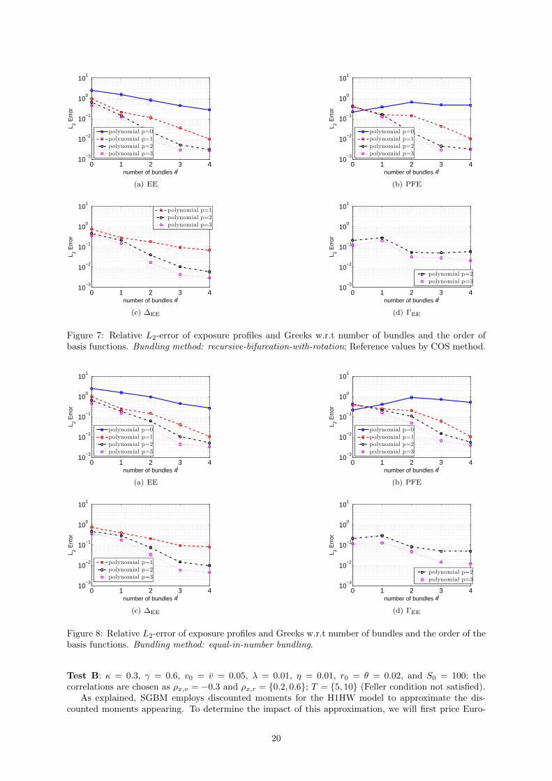
The COS method is an efficient and accurate method for pricing Bermudan options based on Fouriercosine expansion [21]. We adapted the COS method in [21] so that it can also be applied for computingexposure profiles, see also [4]. With the COS method as our reference, we study the convergence of EEand PFE and the EE Greeks.

In Figures 7 and 8, we present the accuracy of SGBM for exposure quantities w.r.t the type ofbundling, the number of bundles and the order of the basis functions. We check the difference of EE,PFE, ∆EE, and ΓEE between the SGBM and COS methods. When the basis function set only includesthe constant p = 0, then all derivatives w.r.t the initial asset value or variance value are equal to zero,and we cannot determine the Greeks values at all. When the basis functions are of order 1, then wecan calculate the first-derivative w.r.t the initial asset value, but the second-derivatives values of thesefunctions are zero.

The bundling method in Figure 7 is recursive-bifurcation-with-rotation, while the results equal-in-number bundling in Figure 8 are very similar.

Unless stated otherwise, recursive-bifurcation-with-rotation bundling is employed in the experimentsto follow.

It is clear that increasing the number of bundles and/or the order of the basis functions can enhancethe accuracy of the results; The impact of the polynomial order on the accuracy becomes smaller whenthe number of bundles increases. With J = 44 bundles and p = 2 the results are as highly satisfactoryas the approximations by p = 3.

In particular, we see that by a higher polynomial order p and a larger number of bundles the accuracyof the Greek values increases. When the number of bundles is sufficiently large (43), basis functions oforder p = 2 perform as well as p = 3 for ∆EE, but for ΓEE, basis functions of order p = 3 improve theaccuracy.

5.3 SGBM results for the Heston Hull-White model

Here, we will analyze exposure results under the HHW model. For validation of the choices for theSGBM components however we first consider the pricing of options.

Our discretization of the HHW model is based on the QE Heston scheme, combined with an Eulerdiscretization for the interest rates. We employ time step ∆t(QE) = 0.05 and the number of paths usedis N = 5 · 105. The following set of parameters has been used:

19

0 1 2 3 410

−3

10−2

10−1

100

101

number of bundles 4j

L 2 Err

or

polynomial p=0

polynomial p=1

polynomial p=2

polynomial p=3

(a) EE

0 1 2 3 410

−3

10−2

10−1

100

101

number of bundles 4j

L 2 Err

or

polynomial p=0

polynomial p=1

polynomial p=2

polynomial p=3

(b) PFE

0 1 2 3 410

−3

10−2

10−1

100

101

number of bundles 4j

L 2 Err

or

polynomial p=1

polynomial p=2

polynomial p=3

(c) ∆EE

0 1 2 3 410

−3

10−2

10−1

100

101

number of bundles 4j

L 2 Err

or

polynomial p=2

polynomial p=3

(d) ΓEE

Figure 7: Relative L2-error of exposure profiles and Greeks w.r.t number of bundles and the order ofbasis functions. Bundling method: recursive-bifurcation-with-rotation; Reference values by COS method.

0 1 2 3 410

−3

10−2

10−1

100

101

number of bundles 4j

L 2 Err

or

polynomial p=0

polynomial p=1

polynomial p=2

polynomial p=3

(a) EE

0 1 2 3 410

−3

10−2

10−1

100

101

number of bundles 4j

L 2 Err

or

polynomial p=0

polynomial p=1

polynomial p=2

polynomial p=3

(b) PFE

0 1 2 3 410

−3

10−2

10−1

100

101

number of bundles 4j

L 2 Err

or

polynomial p=1

polynomial p=2

polynomial p=3

(c) ∆EE

0 1 2 3 410

−3

10−2

10−1

100

101

number of bundles 4j

L 2 Err

or

polynomial p=2

polynomial p=3

(d) ΓEE

Figure 8: Relative L2-error of exposure profiles and Greeks w.r.t number of bundles and the order of thebasis functions. Bundling method: equal-in-number bundling.

Test B: κ = 0.3, γ = 0.6, v0 = v = 0.05, λ = 0.01, η = 0.01, r0 = θ = 0.02, and S0 = 100; thecorrelations are chosen as ρx,v = −0.3 and ρx,r = 0.2, 0.6; T = 5, 10 (Feller condition not satisfied).

As explained, SGBM employs discounted moments for the H1HW model to approximate the dis-counted moments appearing. To determine the impact of this approximation, we will first price Euro-

20

pean options by SGBM and compare the results obtained by the discounted cash flow plain Monte Carloresults.

As in [12], we also compare the implied volatility values for different strike values to analyze theaccuracy.

Subsequently, we present results for Bermudan options, and confirm the SGBM convergence by thecomparison of the direct and the path estimator.

5.3.1 Pricing European options under the HHW model

Employing SGBM for pricing European options, the problem is easier than pricing Bermudan options,as the option can not be exercised prior to maturity, i.e., for all tm < tM ,

V0(X0) = EQ[VM (XM )D(t0, tM )

∣∣∣∣X0

]= EQ

[EQ[VM (XM )D(tm, tM )

∣∣∣∣Xm

]D(t0, tm)

∣∣∣∣X0

]. (68)

We can thus compute the European option estimate either directly from the discounted averaged optionvalues at time tM ; or we can use intermediate time points, t1, . . . , tm, between t0 and tM to calculate theoption values at the paths in a backward iteration, where the option value at time t0 would be calculatedbased on the option values of all paths at time t1. The latter is an SGBM accuracy test which we performhere.

When the analytic formulas and the SGBM simulation are accurate, there should be no significantdifference between these two approaches. However, as we use approximated HHW discounted momentsderived from H1HW, the size of the time step will have impact on the accuracy of the results. We testthis by choosing three different time steps in SGBM, with ∆t = 0.05, 0.5, 10 (the latter being only onetime step).

Table 4 presents the calculated implied volatility (%) results of MC and SGBM with different timesteps and strike values K = 40, 80, 100, 120, 180 when T = 10. Figure 9 displays the correspondingerrors in the implied volatility results. The reference value is the discounted cash flow results obtainedvia Monte Carlo.

ρx,r Strike Monte Carlo QE SGBM ∆t = 0.05 SGBM ∆t = 0.5 SGBM ∆t = 10

0.2

40 25.96(0.02) 25.96(0.007) 25.98(0.006) 26.09(0.010)80 19.96(0.01) 19.95(0.005) 19.98(0.010) 20.04(0.010)

100 18.35(0.01) 18.34(0.005) 18.38(0.008) 18.40(0.009)120 17.45(0.01) 17.43(0.002) 17.48(0.005) 17.45(0.011)180 17.34(0.03) 17.32(0.007) 17.36(0.004) 17.22(0.016)

0.6

40 26.46(0.03) 26.48(0.006) 26.49(0.005) 26.64(0.013)80 20.71(0.02) 20.70(0.005) 20.75(0.008) 20.86(0.016)

100 19.23(0.01) 19.21(0.002) 19.28(0.008) 19.35(0.013)120 18.42(0.02) 18.39(0.003) 18.48(0.008) 18.49(0.014)180 18.27(0.04) 18.25(0.006) 18.34(0.005) 18.26(0.017)

Table 4: Implied volatility (%) results of Monte Carlo method and SGBM method. Number of bundlesJ = 64 and polynomial order p = 2. Test B with T = 10.

The table and figure show that when we take more time steps between t0 and tM , the results becomemore accurate. However, the results with larger time steps are also highly satisfactory. We can thusenhance the accuracy of the SGBM by using more time steps, but this will reduce the method’s efficiency.

5.3.2 Exposure profiles of Bermudan options under HHW model

We now price a Bermudan put option which can be exercised at 10 equally-space exercise date beforematurity T . The strike is set to K = 100. We use the parameters from Test B, with ρx,r = 0.2, andT = 5 and ρx,r = 0.6, and T = 10 respectively.

We test the convergence of SGBM by comparing the direct estimator and the path estimator. Thecomparison of option value convergence with SGBM basis functions of different order is made in Figure10. Figure 11 then shows the SGBM convergence of the difference of the EE values obtained by thedirect and path estimators, when p = 1 and p = 2 w.r.t the number of bundles. The results indicate that

21

0 50 100 150 2000

0.05

0.1

0.15

0.2

Strike

Err

or o

f im

plie

d vo

latil

ity

SGBM, ∆t = 0.05SGBM, ∆t = 0.5SGBM, ∆t = 10

(a) ρx,r = 0.2

0 50 100 150 2000

0.05

0.1

0.15

0.2

Strike

Err

or o

f im

plie

d vo

latil

ity

SGBM, ∆t = 0.05SGBM, ∆t = 0.5SGBM, ∆t = 10

(b) ρx,r = 0.6

Figure 9: Error of the implied volatility (%) vs. strike values. obtained via the same results in Table 4.Reference values: Monte Carlo results.

approximation by p = 2 is favorable, and the number of bundles is best set to 83 = 512. The differencein the EE values of the direct and path estimator decreases with an increasing number of bundles. TheseHHW results support the conclusions in section 5.2 and thus the convergence of the SGBM.

0 1 2 310

12

14

16

18

20

number of bundles 8j

Optionvalue

direct estimator p=1path estimator p=1direct estimator p=2path estimator p=2ErrorbarErrorbar

(a) ρx,r = 0.2, T = 5

0 1 2 314

16

18

20

22

24

26

number of bundles 8j

Optionvalue

direct estimator p=1path estimator p=1direct estimator p=2path estimator p=2ErrorbarErrorbar

(b) ρx,r = 0.6, T = 10

Figure 10: Comparison of option values by the direct estimator and path estimator, when p = 1 andp = 2. Test B with T = 10.

0 1 2 310

−3

10−2

10−1

100

number of bundles 8j

differen

ce

p=1p=2

(a) ρx,r = 0.2, T = 5

0 1 2 310

−3

10−2

10−1

100

The number of bundles 8j

differen

ce

p=1p=2

(b) ρx,r = 0.6, T = 10

Figure 11: Comparison of EE values obtained by the SGBM direct estimator and path estimator, whenp = 1 and p = 2.

For comparison purposes, we also present the corresponding converged results at time t0 in Table 5.We also present the CVA value computed by Equation (9).

5.4 Pricing barrier options and the accuracy

In this subsection, we present results for a knock-out barrier put option under the Heston and HHWmodels, with barrier level H = 0.8S0. Basis functions of order p = 2 are chosen for calculation so that

22

SGBM direct(std.) SGBM path(std.)

ρx,r = 0.2, T = 5

V (0) 11.3747( 6.5e-04) 11.3507(1.5e-02)∆EE(0) -0.2935( 3.0e-05) -ΓEE(0) 0.0143(3.6e-05) -

CVA 0.9829(3.1e-03) -

ρx,r = 0.6, T = 10

V (0) 15.9162(1.28e-02) 15.9310(1.9e-03)∆EE(0) -0.2608(6.39e-04) -ΓEE(0) 0.0085(2.08e-05) -

CVA 2.9678(3.42e-03) -

Table 5: Values of option, Greeks and CVA; Bermudan put option; SGBM based on 5 simulations.

we obtain accurate sensitivities when applying SGBM. The reference values are obtained by the COSmethod for the Heston model. For the HHW model, we use the discounted cash flow Monte Carlo resultsas a reference. If the path does not hit the barrier, the cash flow is equal to the payoff at the maturity;otherwise the option is knocked out at a path and the cash flow is zero.

Under the Heston model, with the parameters from Test A, Figure 12 confirms the convergence ofSGBM by plotting the L2-error of the exposure and their Greek values for barrier options w.r.t thenumber of bundles under the Heston model, where COS method is available for the reference values.The corresponding values are presented in Table 6.

0 1 2 3 410

−4

10−3

10−2

10−1

100

number of bundles 4j

L 2 Err

or

EEPFE

(a) Exposure: EE and PFE

0 1 2 3 410

−3

10−2

10−1

100

101

number of bundles 4j

L 2 Err

or

∆

Γ

(b) Greeks:∆EE and ΓEE

Figure 12: Relative L2-error of the exposure and Greeks for a barrier option. Parameters of Test Aunder the Heston model.

COS SGBM direct(std.) Monte Carlo(std.)

V (0) 1.2300 1.2299(1.8e-03) 1.2283(4.9e-03)∆EE(0) -0.0605 -0.0609(1.2e-04) -ΓEE(0) 0.0031 0.0020(3.3e-05) -

CVA 0.0363 0.0363(8.7e-05) 0.0362(1.4e-04)

Table 6: Values of option, Greeks and CVA; knocked-out barrier put option; SGBM and MC based on5 simulations. Parameters of Test A under the Heston model.

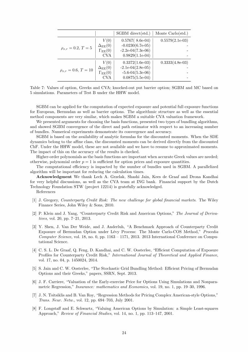
For the HHW model computations, we use the parameters in Test B, and the resulting values aregiven in Table 7.

6 Conclusion

In this paper we have applied the Stochastic Grid Bundling Method (SGBM) for the computation ofexposure profiles and Greek values for asset dynamics with stochastic volatility and stochastic interestrate.

23

SGBM direct(std.) Monte Carlo(std.)

ρx,r = 0.2, T = 5

V (0) 0.5767( 8.6e-04) 0.5579(2.1e-03)∆EE(0) -0.0230(6.7e-05) -ΓEE(0) -2.2e-04(7.3e-06) -

CVA 0.9829(1.1e-04) -

ρx,r = 0.6, T = 10

V (0) 0.3372(1.6e-03) 0.3333(4.8e-03)∆EE(0) -2.1e-04(2.8e-05) -ΓEE(0) -5.6-04(5.3e-06) -

CVA 0.0875(5.5e-04) -

Table 7: Values of option, Greeks and CVA; knocked-out put barrier option; SGBM and MC based on5 simulations. Parameters of Test B under the HHW model.

SGBM can be applied for the computation of expected exposure and potential full exposure functionsfor European, Bermudan as well as barrier options. The algorithmic structure as well as the essentialmethod components are very similar, which makes SGBM a suitable CVA valuation framework.

We presented arguments for choosing the basis functions, presented two types of bundling algorithms,and showed SGBM convergence of the direct and path estimator with respect to an increasing numberof bundles. Numerical experiments demonstrate its convergence and accuracy.

SGBM is based on the availability of analytic formulas for the discounted moments. When the SDEdynamics belong to the affine class, the discounted moments can be derived directly from the discountedChF. Under the HHW model, these are not available and we have to resume to approximated moments.The impact of this on the accuracy of the results is checked.

Higher-order polynomials as the basis functions are important when accurate Greek values are needed;otherwise, polynomial order p = 1 is sufficient for option prices and exposure quantities.

The computational efficiency is impacted by the number of bundles used in SGBM. A parallelizedalgorithm will be important for reducing the calculation times.

Acknowledgment We thank Lech A. Grzelak, Shashi Jain, Kees de Graaf and Drona Kandhaifor very helpful discussions, as well as the CVA team at ING bank. Financial support by the DutchTechnology Foundation STW (project 12214) is gratefully acknowledged.

References

[1] J. Gregory, Counterparty Credit Risk: The new challenge for global financial markets. The WileyFinance Series, John Wiley & Sons, 2010.

[2] P. Klein and J. Yang, “Counterparty Credit Risk and American Options,” The Journal of Deriva-tives, vol. 20, pp. 7–21, 2013.

[3] Y. Shen, J. Van Der Weide, and J. Anderluh, “A Benchmark Approach of Counterparty CreditExposure of Bermudan Option under Levy Process: The Monte Carlo-COS Method,” ProcediaComputer Science, vol. 18, no. 0, pp. 1163 – 1171, 2013. 2013 International Conference on Compu-tational Science.

[4] C. S. L. De Graaf, Q. Feng, D. Kandhai, and C. W. Oosterlee, “Efficient Computation of ExposureProfiles for Counterparty Credit Risk,” International Journal of Theoretical and Applied Finance,vol. 17, no. 04, p. 1450024, 2014.

[5] S. Jain and C. W. Oosterlee, “The Stochastic Grid Bundling Method: Efficient Pricing of BermudanOptions and their Greeks,” papers, SSRN, Sept. 2013.

[6] J. F. Carriere, “Valuation of the Early-exercise Price for Options Using Simulations and Nonpara-metric Regression,” Insurance: mathematics and Economics, vol. 19, no. 1, pp. 19–30, 1996.

[7] J. N. Tsitsiklis and B. Van Roy, “Regression Methods for Pricing Complex American-style Options,”Trans. Neur. Netw., vol. 12, pp. 694–703, July 2001.

[8] F. Longstaff and E. Schwartz, “Valuing American Options by Simulation: a Simple Least-squaresApproach,” Review of Financial Studies, vol. 14, no. 1, pp. 113–147, 2001.

24

[9] L. Stentoft, “Value Function Approximation or Stopping time Approximation: a Comparison ofTwo Recent Numerical Methods for American Option Pricing Using Simulation and Regression,”Journal of Computational Finance, vol. 18, pp. 1–56, 2010.

[10] M. Broadie, P. Glasserman, and Z. Ha, “Pricing American Options by Simulation Using a StochasticMesh with Optimized Weights,” in Probabilistic Constrained Optimization (S. Uryasev, ed.), vol. 49of Nonconvex Optimization and Its Applications, pp. 26–44, Springer US, 2000.

[11] P. Glasserman and B. Yu, “Simulation for American Options: Regression Now or Regression Later?,”in Monte Carlo and Quasi-Monte Carlo Methods 2002 (H. Niederreiter, ed.), pp. 213–226, SpringerBerlin Heidelberg, 2004.

[12] L. Grzelak and C. Oosterlee, “On the Heston Model with Stochastic Interest Rates,” SIAM Journalon Financial Mathematics, vol. 2, no. 1, pp. 255–286, 2011.

[13] M. Pykhtin and S. Zhu, “A Guide to Modelling Counterparty Credit Risk,” GARP Risk Review,pp. 16–22, July/August 2007.

[14] D. Brigo, “Counterparty Risk FAQ: Credit VaR, PFE, CVA, DVA, Closeout, Netting, Collateral, Re-hypothecation, WWR, Basel, Funding, CCDS and Margin Lending,” Papers 1111.1331, arXiv.org,Nov. 2011.

[15] D. Lamberton and B. Lapeyre, Introduction to Stochastic Calculus Applied to Finance, SecondEdition. Chapman & Hall/CRC Financial Mathematics Series, Taylor & Francis, 1996.

[16] M. Larson and F. Bengzon, “Piecewise Polynomial Approximation in 1D,” in The Finite ElementMethod: Theory, Implementation, and Applications, vol. 10 of Texts in Computational Science andEngineering, pp. 1–22, Springer Berlin Heidelberg, 2013.

[17] E. Clement, D. Lamberton, and P. Protter, “An Analysis of a Least Squares Regression Method forAmerican Option Pricing,” Finance and Stochastics, p. 2002.

[18] M. Broadie and M. Cao, “Improved Lower and Upper Bound Algorithms for Pricing AmericanOptions by Simulation,” Quantitative Finance, vol. 8, no. 8, pp. 845–861, 2008.

[19] M. Larson and F. Bengzon, “Piecewise Polynomial Approximation in 2D,” in The Finite ElementMethod: Theory, Implementation, and Applications, vol. 10 of Texts in Computational Science andEngineering, pp. 45–69, Springer Berlin Heidelberg, 2013.

[20] L. B. G. Andersen, “Simple and Efficient Simulation of the Heston Stochastic Volatility Model,”Journal of Computational Finance, vol. 11, pp. 1–48, 2008.

[21] F. Fang and C. Oosterlee, “A Fourier-Based Valuation Method for Bermudan and Barrier Optionsunder Heston’s Model,” SIAM Journal on Financial Mathematics, vol. 2, no. 1, pp. 439–463, 2011.

25

Appendices

A Proofs

A.1 Proof of proposition 1

Here we provide the proof of Proposition 1.

‖cm − cm‖2L2(Im)

=

∫Im

(EQ[Vm+1 (Xm+1) ·D(tm, tm+1)

∣∣∣∣Xm

]− EQ

[Vm+1 (Xm+1) ·D(tm, tm+1)

∣∣∣∣Xm

])2

dXm

≤∫Im

(EQ[(Vm+1 (Xm+1)− Vm+1 (Xm+1)

)2

· (D(tm, tm+1))2

∣∣∣∣Xm

])dXm

≤∫Im

(EQ[(Vm+1 (Xm+1)− Vm+1 (Xm+1)

)2∣∣∣∣Xm

])dXm

≤∫Im

∫Im+1

(Vm+1 (Xm+1)− Vm+1 (Xm+1)

)2

f (Xm+1; Xm) dXmdXm+1

≤∫Im+1

(Vm+1 (Xm+1)− Vm+1 (Xm+1)

)2(∫

Im

f (Xm+1; Xm) dXm

)dXm+1

≤

(∫Im+1

(Vm+1 (Xm+1)− Vm+1 (Xm+1)

)2

dXm+1

)·

(∫Im+1

(∫Im

f (Xm+1; Xm) dXm

)dXm+1

)= (1− ε)‖Vm+1 − Vm+1‖2L2(Im+1) · h(Im), (69)

where h(Im) is the size of the domain Im, as∫Im+1

∫Im

f (Xm+1; Xm) dXmdXm+1

=

∫Im

∫Im+1

f (Xm+1; Xm) dXm+1dXm =

∫Im

(1− ε)dXm = (1− ε)h(Im). (70)

A.2 Proof of proposition 2

We approximate function f(x) by a polynomial f(x) of order p on interval I, where the residual value isdefined as

ep(x) := f(x)− f(x), x ∈ I. (71)

Notice that e(p+1)p (x) = f (p+1)(x) as f (p+1)(x) = 0.

The error of the ’best’ estimation in L2 sense can be bounded when f(x) is p+ 1 times differentiable.Choose p+ 1 distinct points, x0,0, x0,1, . . . , x0,p ∈ I, and apply interpolation, ∀x ∈ I, ∃ η(x) ∈ I, suchthat

ep(x) =f (p+1)(η(x))

(n+ 1)!

p∏i=0

(x− x0,i). (72)

This implies that we can find a polynomial, such that the residual function ep(x0,0) = ep(x0,1) =· · · = ep(x0,p). By Rolle’s theorem, points x1,0, x1,1, . . . , x1,p−1 exist, so that the first derivativee(1)(x1,0) = e(1)(x1,1) = · · · = e(1)(x1,p−1) = 0. By induction, ∀r ≤ p, there exist p − r + 1 pointsxr,0, xr,1, . . . , xr,p−r, From the fundamental theorem of calculus,∀r ≤ p, we have that for any point yin I,

e(r)p (y) = e(r)

p (xr,0) +

∫ y

xr,0

e(r+1)p (x)dx. (73)

26

As e(r)p (xr,0) = 0, we have following

e(r)p (y) =

∫ y

xr,0

e(r+1)p (x)dx ≤

∫ y

xr,0

∣∣e(r+1)p (x)

∣∣dx≤∫ y

xr,0

∣∣1∣∣ · ∣∣e(r+1)p (x)

∣∣dx ≤ (∫ y

xr,0

∣∣1∣∣2dx) 12(∫ y

xr,0

∣∣e(r+1)p (x)

∣∣2dx) 12

≤ h 12 ‖e(r+1)

p ‖L2(I). (74)

When we square both sides, we obtain(e(r)p (y)

)2

≤ h‖e(r+1)p ‖2L2(I), (75)

and as a result, the L2 norm of e(r)p (y) in interval I is given by,

‖e(r)p ‖L2(I) =

(∫I

(e(r)p (y)

)2

dy

) 12

≤(∫

I

h‖e(r+1)p ‖2L2(I)dy

) 12

≤ h‖e(r+1)p ‖L2(I). (76)

By induction, it is easy to find that

‖ep‖L2(I) ≤ h‖e(1)p ‖L2(I) ≤ · · · ≤ hp+1‖e(p+1)

p ‖L2(I) = hp+1‖f (p+1)‖L2(I) (77)

B The joint discounted characteristic functions

In this appendix we provide the reader with known results about characteristic function. Based on these,it is easy to determine (either by hand or by a computer program) the discounted moments, needed inSGBM.

B.1 Heston model

The expression for the discounted ChF of the Heston model is given by[21]:

Φ(u1, u2, T |Xt) = exp(A(u1, u2, τ) + B(u1, τ)xt + C(u1, u2, τ)vt

), (78)

where,

A(u1, u2, τ) = I1 + I2, B(u1, τ) = iu1,

C(u1, u2, τ) = r+ −2D1

γ2 (1− ge−D1τ ),

(79)

where

g =iu2 − r−iu2 − r+

, D1 =

√(κ− γρx,viu1)

2+ γ2u1(u1 + i),

r± =1

γ2(κ− γρx,viu1 ±D1) , (80)

and

I1 = κv

(r−τ −

2

γ2log

(1− ge−D1τ

1− g

)), I2 = r(iu1 − 1)τ.

27

B.1.1 Discounted moments

The analytic formulas for the discounted moments and their first and second derivatives are obtainedwith symbolic calculations in MATLAB. We will present the discounted moments for the Heston model.

EQ [xT ·D(t, T )|Xt] =

(xt +

1

2κ(v − vt)

(1− e−κτ

)+ (r − 1

2v)τ

)e−rτ , (81)

EQ [x2T ·D(t, T )|Xt

]=

((xt +

1

2κ(v − vt)

(1− e−κτ

)+

(r − 1

2v

)τ

)2

+v

8κ3Ω1 +

vt4κ3

Ω2

)e−rτ , (82)

EQ [vT ·D(t, T )|Xt] =(v + (vt − v) e−κτ

)e−rτ , (83)

EQ [v2T ·D(t, T )|Xt

]=

(vtγ

2

κ

(e−κτ − e−2κτ

)+vγ2

2κ

(1− e−κτ

)2+(v + (vt − v) e−κτ

)2)e−rτ , (84)

EQ [xT · vT ·D(t, T )|Xt] =

((v + (vt − v) e−κτ )

(xt +

1

2κ(v − vt) (1− e−κτ ) + (r − 1

2v)τ

)

+vγ2

4κ2Ω3 +

vtγ2

2κ2Ω4

)e−rτ , (85)

with Xt = [xt, vt]T , τ = T − t, where

Ω1 =e−2κτγ2 + 4e−κt((1 + κτ)γ2 − 2ρκγ (2 + κt) + 2κ2

)+ (2κτ − 5) γ2

− 8ρκγ (κτ − 2) + 8κ2 (κτ − 1) , (86)

Ω2 =− e−2κτγ2 + 2e−κτ(−κτγ2 + 2ρκγ (1 + κτ)− 2κ2

)+ γ2 − 4κργ + 4κ2, (87)

Ω3 =e−2κτ + 2κe−κτ (τ − 2ρ

γ(1 + κτ)) +

4κρ− γγ

, (88)

Ω4 =e−κτ(

1− κτ +2ρκ2τ

γ

)− e−2κτ . (89)

B.2 Black-Scholes-Hull-White model

The expression for discounted ChF of the BSHW model is given by:

Φ(u1, u2, u3, T |Xt) = exp(A(u1, u2, w, τ) + B(u1, τ)xt + D(u1, u3, τ)rt

), (90)

with B(u1, τ) as in B.1, and

A(u1, u2, u3, τ) = I1 + I2 + I3 + I4, D(u1, u3, τ) =iu1 − 1

λ

(1− e−λτ

)+ iu3e

−λτ ,

(91)

and

I1 =1

2σ2iu1(iu1 − 1)τ,

I2 = θ

((iu1 − 1)τ +

1

λ(e−λτ − 1)(iu1 − 1)− iu3

(e−λτ − 1

)),

I3 =η2

2λ2

(2

λ(u1 + i)(e−λτ − 1)(λu3 − u1 − i) +

1

2λ

(e−2λτ − 1

)(λu3 − u1 − i)2 − (u1 + i)2τ

),

I4 =ηθσρx,r

λ

(− iu1 + u2

1

λ(λτ + e−λτ − 1) + u1u3(e−λτ − 1)

). (92)

Again the discounted moments are obtained by symbolic computations in MATLAB.

28

B.3 H1HW model

The expression for the discounted ChF for the approximate HHW model, called the H1HW model, isgiven by[12]:

Φ(u1, u2, u3, T |Xt) = exp(A(u1, u2, u3, τ) + B(u1, τ)xt + C(u1, u2, τ)vt + D(u1, u3, τ)rt

), (93)

where the coefficients B(u1, τ), C(u1, u2, τ) and D(u1, u3, τ) are the same in sections B.1 and B.2, and

A(u1, u2, u3, τ) = I1 + I2 + I3 + I4, (94)

where expressions g, D1 and r± are the same one as for the Heston model, and

I1 = θ

((iu1 − 1)τ +

1

λ(e−λτ − 1)(iu1 − 1)− iu3

(e−λτ − 1

)), (95)

I2 = κv

(r−τ −

2

γ2log

(1− ge−D1τ

1− g

)),

I3 =η2

2λ2

(2

λ(u1 + i)(e−λτ − 1)(λu3 − u1 − i) +

1

2λ

(e−2λτ − 1

)(λu3 − u1 − i)2 − (u1 + i)2τ

),

I4 = ηρx,r

(− iu1 + u2

1

λG1(τ, vt)− u1u3G2(τ, vt)

). (96)

The two integrals appearing above are computed numerically as

G1(τ, vt) :=

∫ τ

0

E[√vT−s

∣∣vt] (1− e−λs) ds ≈ L−1∑k=0

E[√v(T−k∆s)

∣∣vt] (1− e−λ(k∆s))

∆s, (97)

G2(τ, vt) :=

∫ τ

0

E[√vT−s

∣∣vt] e−λsds ≈ L−1∑k=0

E[√v(T−k∆s)

∣∣vt] (e−λ(k∆s))

∆s, (98)

where τ = T − t, ∆s = τL , L is the number of integration intervals and the conditional expectation of

the square root of the variance is given by (59).

29