monetary dynamics in a general equilibrium version of the ...epge.fgv.br/files/1687.pdf · monetary...
TRANSCRIPT
Monetary Dynamics in a General Equilibrium
Version of the Baumol-Tobin Model
André C. Silva∗
July, 2004
Abstract
I study the welfare cost of inflation and the effect on prices after a perma-
nent increase in the interest rate. In the steady state, the real money demand is
homogeneous of degree one in income and its interest-rate elasticity is approx-
imately equal to −1/2. Consumers are indifferent between an economy with10% p.a. inflation and one with zero inflation if their income is 1% higher in
the first economy. A permanent increase in the interest rate makes the price
level to drop initially and inflation to adjust slowly to its steady state level.
∗Email: [email protected], [email protected] (after September 2004). I have greatly benefited
from comments by the members of my thesis committee: Fernando Alvarez, Lars P. Hansen, Robert
E. Lucas, Jr. and Hanno Lustig. I am specially grateful to the Chairman, Fernando Alvarez for
suggestions and encouragement. I have also benefited from comments by Rodrigo Bueno, Francisco
Buera, Vasco Carvalho, Raphael de Coninck, Rubens Cysne, Jean-Pierre Dube, Julio Elias, Alejan-
dro Rodriguez and the members of the Economic Dynamics Working Group at the University of
Chicago. I thank Donour Sizemore for discussions on the computer program used in section 5. All
errors are my own.
1
1. INTRODUCTION
This paper offers a monetary model with two applications: to measure the welfare
cost of inflation, and to analyze the behavior of prices after an interest rate shock. The
link between inflation and welfare is the deviation of resources from consumption to
the management of money. Prices are flexible, but they do not adjust instantaneously
to a change in the nominal interest rate.
As in Baumol (1952) and Tobin (1956), money is useful for transactions but agents
incur a transfer cost whenever they exchange bonds for money. Moreover, money
holdings do not receive interest. The economy has infinitely-lived consumers with
different endowments and constant relative risk aversion utility. The utility function
is in terms of goods only: neither money nor the transfer cost enter in the utility
function.
The analysis offers two contributions. The first is to measure the welfare cost of
inflation for different preference parameters with infinitely-lived consumers, consump-
tion smoothing, and transfer cost in goods. The second is to describe the behavior of
prices after a permanent increase in the nominal interest rate.
The welfare cost of inflation is defined as the income compensation required to
leave consumers indifferent between an economy under positive interest rate and one
with zero interest rate. According to the model, consumers are indifferent between
an economy with 10% p.a. inflation and an economy with zero inflation if the income
of each consumer is 1% higher in the first economy. This estimate agrees with the
findings in Lucas (2000). The elasticity of intertemporal substitution has a small
effect on the welfare cost of inflation. The model is calibrated using U.S. data from
1900 to 1997.
When the nominal interest rate is positive, agents use their resources to maintain
the optimal level of money holdings. An increase in the interest rate decreases average
2
consumption and increases the variation of consumption. The first effect happens
because agents exchange bonds for money more frequently. The second effect is a
consequence of the concentration of consumption in the beginning of each holding
period.
The optimal monetary policy is to decrease the money supply at the rate of time
preferences and set the nominal interest rate to zero, as in Friedman (1969). When
the nominal interest rate decreases towards zero, money demand converges to the
present value of production discounted by the intertemporal discount rate.
We also study a 1% permanent increase in the nominal interest rate in an economy
initially in the steady state with zero inflation. This shock produces an initial price
drop and then a period of around 5 months with inflation under 1% p.a. After this
period, inflation starts to vary between 5% and −3% p.a. in cycles of about 6 months.Eventually, inflation approaches its new steady state value of 1% p.a.
General equilibrium versions of the Baumol-Tobin model were also presented by
Jovanovic (1982), Romer (1986), and Fusselman and Grossman (1989). In Jovanovic,
consumption is assumed constant within holding periods. As a result, the optimal
interval between transfers is finite even when the nominal interest rate is zero. There-
fore, zero interest rate minimizes the welfare cost, but it does not reduce it to zero.
In Romer, the economy is populated by consumers with finite life and zero intertem-
poral discount factor. Jovanovic and Romer do not calculate the welfare cost and
they do not study a shock to the nominal interest rate. Fusselman and Grossman
consider agents with logarithmic utility and transfer cost in utility terms. They have
a different calibration and they do not discuss the welfare cost of inflation. With
transfer cost in utility terms, the path of prices in their model does not converge to
a new steady state after a nominal interest rate shock.
Romer (1987) studies the effect on money demand after a permanent change in the
nominal interest rate using the framework in Romer (1986). But he keeps the real
3
interest fixed during the transition. Here, the real interest rate varies after the shock
because the price level does not change instantaneously with the nominal interest
rate.
The framework in this paper is adapted from the formulation in Grossman (1987).
In this model, agents exchange bonds for money in fixed periods. I include the decision
of the optimal interval between transfers1. As in Alvarez, Atkeson and Edmond
(2002), agents keep their resources in two separate accounts: one for the goods market
and another one for the asset market.
The structure of the remaining of the paper is the following. Section 2 contains the
description of the economy and the utility maximization problem. Section 3 has the
analysis of the economy in the steady state. Section 4 contains the measurement of
the welfare cost of inflation. Section 5 has the study of the effects of a change in the
nominal interest rate. Section 6 concludes. All proofs are in the appendix.
2. THE MODEL
The model consists of a continuum of consumers who need to use money for goods
transactions and who incur a cost to transfer resources from the asset market to
the goods market. The transfer cost is paid in goods. It covers administrative,
opportunity, and non-pecuniary costs involved in making a transfer, as motivated by
Baumol (1952) and Tobin (1956). Time is continuous2. The model is adapted from
Grossman (1987)3.
1The possibility of paying a proportional transaction cost between holding periods is removed. I
use the same notation as in Grossman (1987) whenever possible.2This is a simplifying assumption. It allows us to ignore integer constraints to find the optimal
interval between transfers.3In Grossman (1987), the interval between transfer is fixed and the derivation of the steady state
is obtained supposing that agents equalize their marginal utility of wealth. The characterization of
the steady state is done here explicitly as a function of the endowments.
4
Consumers are infinitely-lived and they discount the future at the rate ρ > 0.
They choose how much to consume and the time of each transfer. Let c (t) denote
consumption at time t and Nj ≥ 0 j = 1, 2, ... denote the interval between transfers.The time of each transfer is given by the summation of the intervals Nj, define thus
Tj ≡Pj
s=1Nj, T0 ≡ 0. Each Tj denotes the time in which a transfer is made.
Consumers have preferences given by
U (c) =∞Xj=0
Z Tj+1
Tj
e−ρtu (c (t)) dt. (1)
The utility function is assumed to have the constant relative risk aversion form,
u (c) =
c1−σ
1− σfor σ 6= 1, σ > 0,
log c for σ = 1.
This family of preferences will generate an aggregate real money demand linear in
income. Preferences are a function of goods only: neither money nor the transfer cost
enter in the utility function4.
Each agent owns two accounts: a brokerage account and a bank account. The
brokerage account contains all resources used in the asset market. The bank account
contains the monetary resources used for goods purchases.
There is a single and nonstorable good. Each consumer produces Y units of the
good in every period. Consumption goods are traded in the goods market. The price
level at time t is given by P (t) and inflation is given by π (t). Taxes at each time t
are denoted by τ (t). Taxes are lump sum and are levied in the brokerage account.
At each time, production is sold in the goods market and the proceeds after taxes are
deposited in the brokerage account. Although the good is sold in the goods market
for money, agents cannot use this money to buy goods in the same period5.4Since the model is deterministic, we will make reference to the elasticity of intertemporal sub-
stitution 1/σ.5It is interesting to view an agent as a family composed of two types of individuals, a worker and
5
In order to transfer resources from the brokerage account to the bank account,
agents have to pay a fee in goods. The transfer cost is proportional to income, it
is given by γY , γ > 0. A value γ = 1 means that the transfer cost is equal to one
working day per transfer.
Government bonds are traded in the asset market. Let Q (t) be the value at time
zero of one dollar to be received at time t. The nominal interest rate is denoted by
r (t) and it is assumed positive in every period.
Let B0 denote bond holdings held by each consumer at time zero and letW0 denote
total wealth initially available in the brokerage account. We have
W0 = B0 +
Z ∞
0
Q (t) [P (t)Y − τ (t)] dt. (2)
All consumers have the same present value of production. Any difference in the
balance of the brokerage accounts across consumers is given by the amount of bonds
held.
At time zero, in addition to the deposits in the brokerage account, agents have M0
in money holdings in the bank account.
What distinguishes consumers in this economy is the pair (M0,W0). There is an
initial given distribution F of M0 and W0 along with its density function f .
The importance of money is given by its transaction role: in order to buy goods,
agents need to use money. Let M (t,M0,W0) denote the quantity of money held at
time t by consumer (M0,W0). Whenever there is a purchase of goods, the amount
of money necessary for the purchase is subtracted from the bank account. Therefore,
the cash in advance constraint in this economy is
M (t,M0,W0) = −P (t) c (t,M0,W0) , t 6= T1, T2, ... (3)
a shopper, as in Lucas (1990). The worker produces the consumption good Y in each period and
deposits the procedures in a brokerage account in the form of bonds. The shopper decides when to
sell bonds for money and how to use the money to buy goods.
6
where c (t,M0,W0) denotes consumption at time t of consumer (M0,W0) and x (t) ≡∂x (t) /∂t.
Notice that M0 can be used promptly for good transactions. In order to use the
balance in the brokerage account to buy goods, however, the agents need to pay
γY , sell a certain amount of bonds and transfer the monetary proceeds to the goods
market.
If it were costless to transfer resources from the asset market to the goods market,
agents would hold only the quantity of money needed to buy goods for each particular
time. The reason is that interest is accrued to bonds in every period whereas it is
not accrued to money. After trading, consumers would have zero money holdings and
they would transfer resources in every period.
A transfer cost induces agents to maintain resources sufficient for consumption in
several periods. Just after the transfer, agents hold a relatively large quantity of
money.
After the first transfer, at time T1, consumers will withdraw the exact amount of
money necessary to consume until the next transfer. Agents use their money holdings
until they exhaust them. When it happens, they make another transfer.
Agents have to decide consumption and money holdings for each time t, and when
they will transfer resources between their accounts. This decision is done at time zero,
given the path of the nominal interest rate and of the price level. Money holdings in
the beginning of each holding period are denoted by M+ (t).
The initial value of money holdings, M0, is exogenously given. It is not necessarily
the amount of money required for consumption between 0 and T1. Agents are, there-
fore, allowed to transfer an amount K ≥ 0 from the bank account to the brokerage
account at time T1. The variable K denotes the quantity of money not used in [0, T1)
and deposited in the brokerage account at t = T16.
6We have K > 0 if M0 is higher than the value otherwise chosen by the agent. This is likely to
7

The individual maximization problem is to maximize (1), subject to (3) and
∞Xj=1
Q (Tj)M+ (Tj) +
∞Xj=1
Q (Tj)P (Tj) γY ≤W0 +Q (T1)K, (4)
Z T1
0
P (t) c (t) +K ≤M0 (5)
plus the nonnegativity constraints for c (t), M (t), Nj, and K7.
The constraint (4) states that the present value of all money transfers is equal to
the present value of the deposits in the brokerage account. The constraint (5) states
that consumption until the first transfer must be financed from M0.
The initial amount of the money supply is given byMS0 . The money supply at time
t is given by MS (t) and its growth rate is given by α (t). The government sets taxes
and issues money in order to finance its real purchases g (t) and the initial quantity
of bonds held by the public BS0 .
The government budget constraint is given by
BS0 +
Z ∞
0
Q (t)P (t) g (t) dt =
Z ∞
0
Q (t) τ (t) dt+
Z ∞
0
Q (t)P (t)MS (t)
P (t)dt. (6)
If the government wants to inject money, it needs to exchange bonds for money with
the consumers in the asset market. The present value of these open market operations
is reflected by the term BS08.
The market clearing conditions for money and bonds are given respectively byZM (t,M0,W0) dF (M0,W0) =MS (t) , (7)
happen if M0 is too high relative to W0 or if inflation is high in the beginning periods. In principle
we would need a variable K for each holding period, Kj . But we know that, with positive nominal
interest rates, the quantity of money will be chosen to make Kj = 0 for j ≥ 2.7I remove the reference to (M0,W0) of these variables to simplify notation when it does not lead
to ambiguity.8Taxes τ (t) and government purchases g (t) are described for completeness. These variables will
be set to zero and bonds will be financed by seigniorage.
8
ZB0 (M0,W0) dF (M0,W0) = BS
0 , (8)
for all t.
We have to take into account the transfer cost to write the market clearing condition
for goods. Let
A (t, δ) ≡ {(M0,W0) : Tj (M0,W0) ∈ [t, t+ δ)}
for a certain j = 1, 2... denote the set of consumers making a transfer during the
interval [t, t+ δ). The measure of A (t, δ) gives the number of transfers from time t
to time t+ δ. The total amount of resources directed to financial transfers at time t
is then given by
γY limδ→0
ZA(t,δ)
1
δdF (M0,W0) . (9)
The market clearing condition for goods is therefore given byZc (t,M0,W0) dF (M0,W0) + g (t) + γY lim
δ→0
ZA(t,δ)
1
δdF (M0,W0) = Y . (10)
Equilibrium in this economy is defined as prices P (t), Q (t), demands c (t,M0,W0),
interval between transfers Nj (M0,W0), government consumption g (t) and taxes τ (t)
such that (i) c (t,M0,W0) solves the maximization problem of each individual (M0,W0),
(ii) the government budget constraint holds, and (iii) the market clearing conditions
for goods, money and bonds hold.
It is interesting to rewrite the individual budget constraint for t ≥ T1 as∞Xj=1
Q (Tj)
Z Tj+1
Tj
P (t) c (t) dt+∞Xj=1
Q (Tj)P (Tj) γY ≤W0 +Q (T1)K.
For this, we use the fact that money holdings are exhausted in the end of each holding
period.
The first order condition with respect to consumption in the interior of a holding
period is given by
e−ρtu0 (c (t)) = λ (M0,W0)Q (Tj)P (t) , Tj < t < Tj+1, j = 1, 2, ..., (11)
9
for consumer (M0,W0)9. λ (M0,W0) is the Lagrange multipliers of the constraint
(4). Notice that, since u is concave, if inflation at time t is greater than or equal
to −ρ then consumption within a holding period is decreasing. Consumers concen-trate consumption in the beginning of a holding period to avoid losing resources for
inflation.
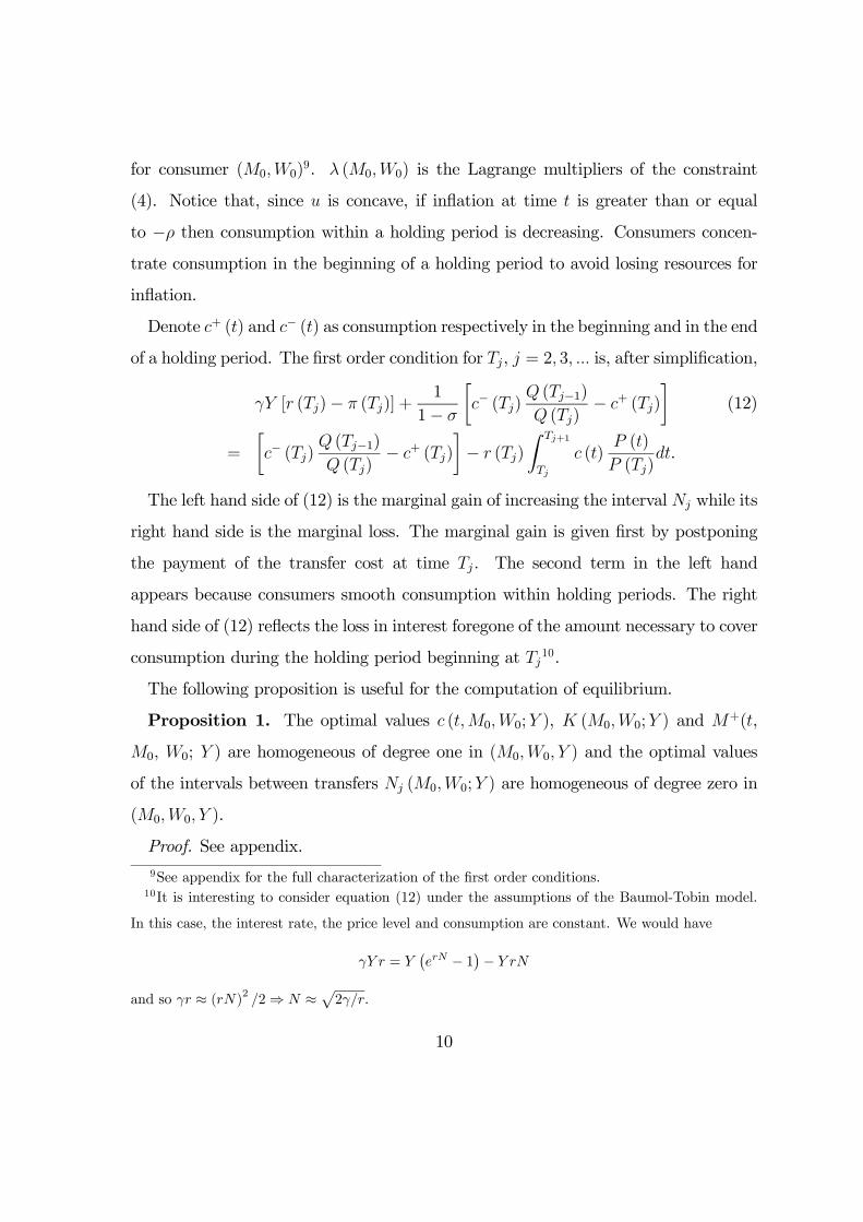
Denote c+ (t) and c− (t) as consumption respectively in the beginning and in the end
of a holding period. The first order condition for Tj, j = 2, 3, ... is, after simplification,
γY [r (Tj)− π (Tj)] +1
1− σ
·c− (Tj)
Q (Tj−1)Q (Tj)
− c+ (Tj)
¸(12)
=
·c− (Tj)
Q (Tj−1)Q (Tj)
− c+ (Tj)
¸− r (Tj)
Z Tj+1
Tj
c (t)P (t)
P (Tj)dt.
The left hand side of (12) is the marginal gain of increasing the interval Nj while its
right hand side is the marginal loss. The marginal gain is given first by postponing
the payment of the transfer cost at time Tj. The second term in the left hand
appears because consumers smooth consumption within holding periods. The right
hand side of (12) reflects the loss in interest foregone of the amount necessary to cover
consumption during the holding period beginning at Tj10.
The following proposition is useful for the computation of equilibrium.
Proposition 1. The optimal values c (t,M0,W0;Y ), K (M0,W0;Y ) and M+(t,
M0, W0; Y ) are homogeneous of degree one in (M0,W0, Y ) and the optimal values
of the intervals between transfers Nj (M0,W0;Y ) are homogeneous of degree zero in
(M0,W0, Y ).
Proof. See appendix.9See appendix for the full characterization of the first order conditions.10It is interesting to consider equation (12) under the assumptions of the Baumol-Tobin model.
In this case, the interest rate, the price level and consumption are constant. We would have
γY r = Y¡erN − 1¢− Y rN
and so γr ≈ (rN)2 /2⇒ N ≈p2γ/r.10
For the proof, we use the linearity of the budget constraints and the fact that the
transfer cost is proportional to income. Since all agents have the same income Y , we
drop this identifier and index the individual solutions by (M0,W0).
3. THE ECONOMY IN THE STEADY STATE
We now describe the economy in the steady state. In this case, the values of the
nominal interest rate and of the inflation rate are constant. Moreover, the interval
between transfers for all consumers are equal. We aggregate individual money hold-
ings and find the aggregate money demand. We find the distribution of M0 and W0
such that the economy is in the steady state since t = 0. The steady state is unique.
The calibration of the transfer cost parameter γ is done so that the steady state
money demand passes through the geometric mean of the nominal interest rates and
of the money-income ratios for U.S. during the period 1900-1997. See appendix for
the description of the data.
Suppose that the monetary authority sets the growth rate of money creation at a
constant α. We look for an equilibrium in which individuals visit the asset market at
constant intervals N2 (M0,W0) = N3 (M0,W0) = ... = N . The values of T1 (M0,W0)
will be different across consumers and they will depend on (M0,W0). The properties
of the economy in the steady state allow us to call the equilibrium of this type a
stationary equilibrium. We need first a formal definition.
Definition 1. A stationary equilibrium is given by prices r, π, demands c (t,M0,W0),
intervals between transfers Nj (M0,W0), j = 1, 2, ..., a distribution F of (M0,W0),
government consumption g (t), and taxes τ (t) such that
i. r (t) = r, π (t) = π;
ii. Nj (M0,W0) = N for all (M0,W0) and j = 2, 3, ... is such that consumers
maximize utility given prices;
iii. the distribution of F (M0,W0) is such that T1 (M0,W0) is uniformly distributed
11
along [0, N);
iv. the market clearing conditions for goods, money and bonds hold;
v. the government budget constraint holds; and
vi. agents have the same consumption pattern along their holding period. That is,
c (T1 (M0,W0) + t,M0,W0) = c (T1 (M00,W
00) + t,M 0
0,W00) , (13)
for all pairs (M0,W0), (M 00,W
00) in the support of F and all t ≥ 0.
Equation (13) states that consumption is the same for two different consumers
if the time elapsed since the first transfer is the same for both consumers. The
only difference across consumers in the stationary equilibrium is their position in the
holding period. In particular, consumption just after a transfer is the same for all
agents. Denote this value by c0. This is also the highest level of consumption within
a holding period.
We now characterize the optimal behavior of a consumer given the individual initial
endowments M0 and W0. Set g (t) = 0 and τ (t) = 0.
We first characterize the decision of Nj (M0,W0), j ≥ 2, and then proceed to thechoice of T1 (M0,W0). We write N (r, ρ, σ, γ) to stress the dependence of the steady
state interval between transfers to the parameters of the model.
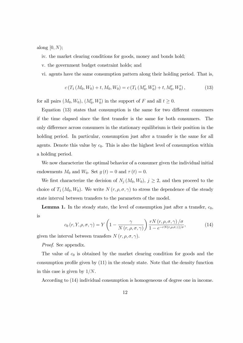
Lemma 1. In the steady state, the level of consumption just after a transfer, c0,
is
c0 (r, Y, ρ, σ, γ) = Y
µ1− γ
N (r, ρ, σ, γ)
¶rN (r, ρ, σ, γ) /σ
1− e−rN(r,ρ,σ,γ)/σ, (14)
given the interval between transfers N (r, ρ, σ, γ).
Proof. See appendix.
The value of c0 is obtained by the market clearing condition for goods and the
consumption profile given by (11) in the steady state. Note that the density function
in this case is given by 1/N .
According to (14) individual consumption is homogeneous of degree one in income.
12
Consumers direct γY/N of their resources to transfers. We need NY > γY to have
positive consumption: production during a holding period must be greater than the
transfer cost paid to obtain money holdings for the same period.
Consider the case in which the elasticity of intertemporal substitution is high and
preferences are close to linear (σ → 0). In this case, the value of N is large and each
agent consumes almost his present value of production in the beginning of the holding
period. So c0 is very large relative to Y and c0/Y → +∞.Proposition 2 gives the value of N (r, ρ, σ, γ). Proposition 3 assures existence and
uniqueness.
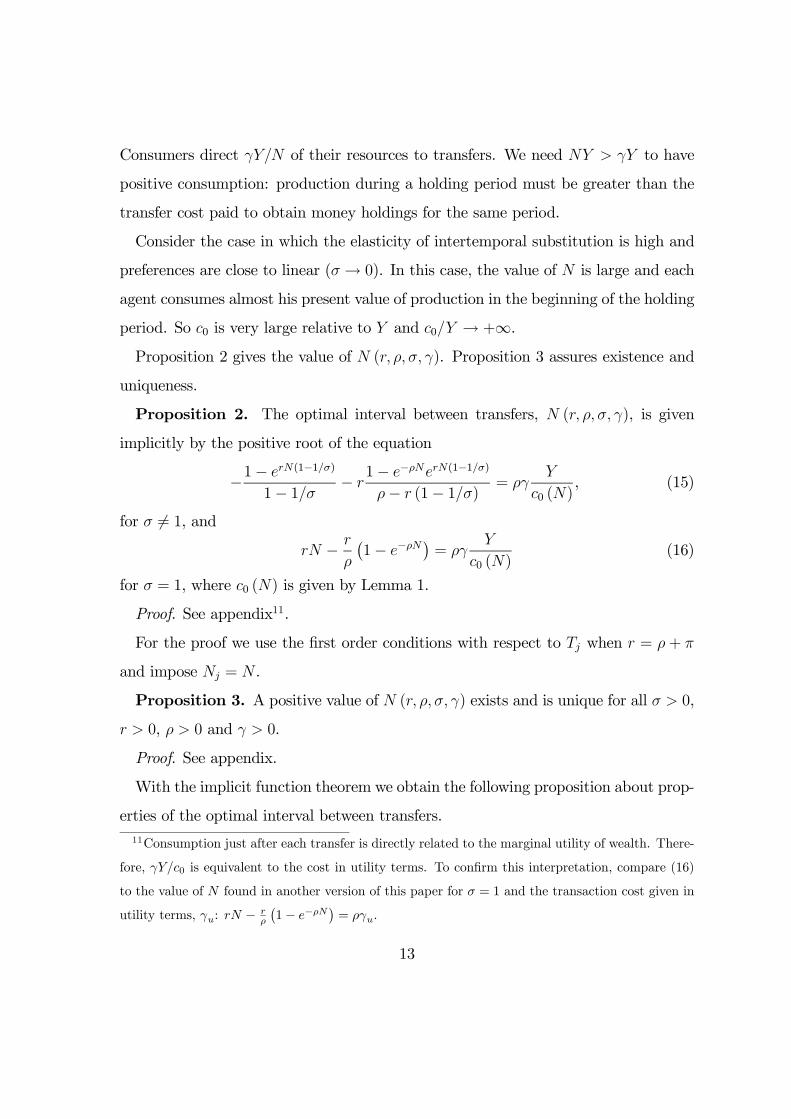
Proposition 2. The optimal interval between transfers, N (r, ρ, σ, γ), is given
implicitly by the positive root of the equation
−1− erN(1−1/σ)
1− 1/σ − r1− e−ρNerN(1−1/σ)
ρ− r (1− 1/σ) = ργY
c0 (N), (15)
for σ 6= 1, andrN − r
ρ
¡1− e−ρN
¢= ργ
Y
c0 (N)(16)
for σ = 1, where c0 (N) is given by Lemma 1.
Proof. See appendix11.
For the proof we use the first order conditions with respect to Tj when r = ρ + π
and impose Nj = N .
Proposition 3. A positive value of N (r, ρ, σ, γ) exists and is unique for all σ > 0,
r > 0, ρ > 0 and γ > 0.
Proof. See appendix.
With the implicit function theorem we obtain the following proposition about prop-
erties of the optimal interval between transfers.11Consumption just after each transfer is directly related to the marginal utility of wealth. There-
fore, γY/c0 is equivalent to the cost in utility terms. To confirm this interpretation, compare (16)
to the value of N found in another version of this paper for σ = 1 and the transaction cost given in
utility terms, γu: rN − rρ
¡1− e−ρN
¢= ργu.
13
Proposition 4. The optimal value of the interval between transfers is such that
(i) ∂N∂r
< 0; (ii) ∂N∂γ
> 0; (iii) ∂N∂ρ
> 0; (iv) N > γ; (v) limγ→0N = 0; (vi) limr→0 rN =
ε > 0.
The interval between transfers is decreasing in the nominal interest rate and in-
creasing in the transfer cost. It increases without bound as the interest rate decreases
towards zero. The product rN , however, converges to a small positive constant when
r goes to zero. We will see that this will make the real money demand bounded when
r goes to zero.
The interval N (r, ρ, σ, γ) goes to zero if the transfer cost goes to zero. We also ob-
tained numerically that it decreases when the elasticity of intertemporal substitution
decreases.
When r and ρ are close to zero, the terms rN and ρN are also close to zero12. With
a second-order Taylor expansion of the terms e−ρN and e−rN(1−σ)/σ we obtain
N2 −Nγ
µ1− 1
σ
¶− 2γ
r= 0.
With r small and σ bounded away from zero, the term 2γ/r is much larger than the
term (1− 1/σ). Therefore, the value of N is approximated by
N ≈r2γ
r.
We have the square-root formula for the interval between transfers13. The elasticity
of intertemporal substitution does not appear in this formula. It reflects the fact that12When σ = 1, limr→0 rN ≈ ργ/(1 + ργ/2) = 1.5× 10⁻⁴ for the parameterization used here. See
the proof of proposition 4 in the appendix for details.
13The approximation is better the higher is the value of σ. For an idea of the degree of the
approximation, the true value of N is higher than the approximated value by 0.3%, 0.4% and 3.7%
respectively for σ = 1, σ = 0.5, and σ = 0.05. The other parameters used in this example were
γ = 1.791, r = 4% p.a. and ρ = 3% p.a. Note that as σ increases then consumption is less variable
and we are closer to the assumptions of the Baumol-Tobin model. Jovanovic (1982) also obtains
14
the interval between transfers is more sensitive to the nominal interest rate and to
the transfer cost.
By proposition 2, the steady state N (r, ρ, σ, γ) does not depend on the initial
conditions M0 and W0, as we need for the stationary equilibrium. The time of the
first visit to the asset market, T1, depends on these values. Proposition 5 gives the
time of the first transfer.
Proposition 5. In the steady state, the first transfer from the brokerage account
to the bank account, T1(r, ρ, σ, γ, M0, W0), is given implicitly by the solution of
rT1 = logλ
µ+ rN ,
where λ (r, ρ, σ, γ,W0, T1) and µ (r, ρ, σ, γ,M0, T1) are the Lagrange multipliers of (4)
and (5) respectively.
Proof. See appendix.
We can now describe the behavior of consumption in the steady state within any
holding period. Let c (x) denote consumption at the position x ∈ [0, N (r, ρ, σ, γ)).In the stationary equilibrium, consumption is periodic. That is, c is such that
c (x) = c [x+ T1 + (j − 1)N,M0,W0]
for all x in [0, N) and for all (M0,W0) in the support of F , j = 1, 2, ... The function
c (x) is given by
c (x) = c0e− rσx, 0 ≤ x < N (r, ρ, σ, γ) ,
where c0 is given by Lemma 1 and Proposition 2.
The ratio of consumption in the beginning of a holding period to consumption in
the end of a holding period, erN/σ, is approximately equal to 1+√2γr/σ. If r is close
the square-root formula as an approximation of his model. Lucas (2000) obtains the square-root
formula with the McCallum-Goodfriend framework, where time and real money balances interact
via a transactions technology.
15
to zero or σ is high, then consumption is approximately constant. If the transfer cost
γ is close to zero then the interval between transfers goes to zero and consumption is
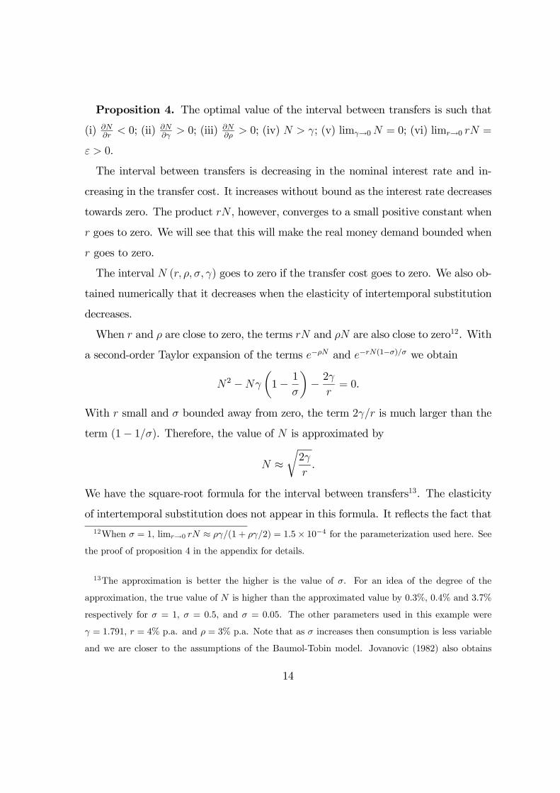
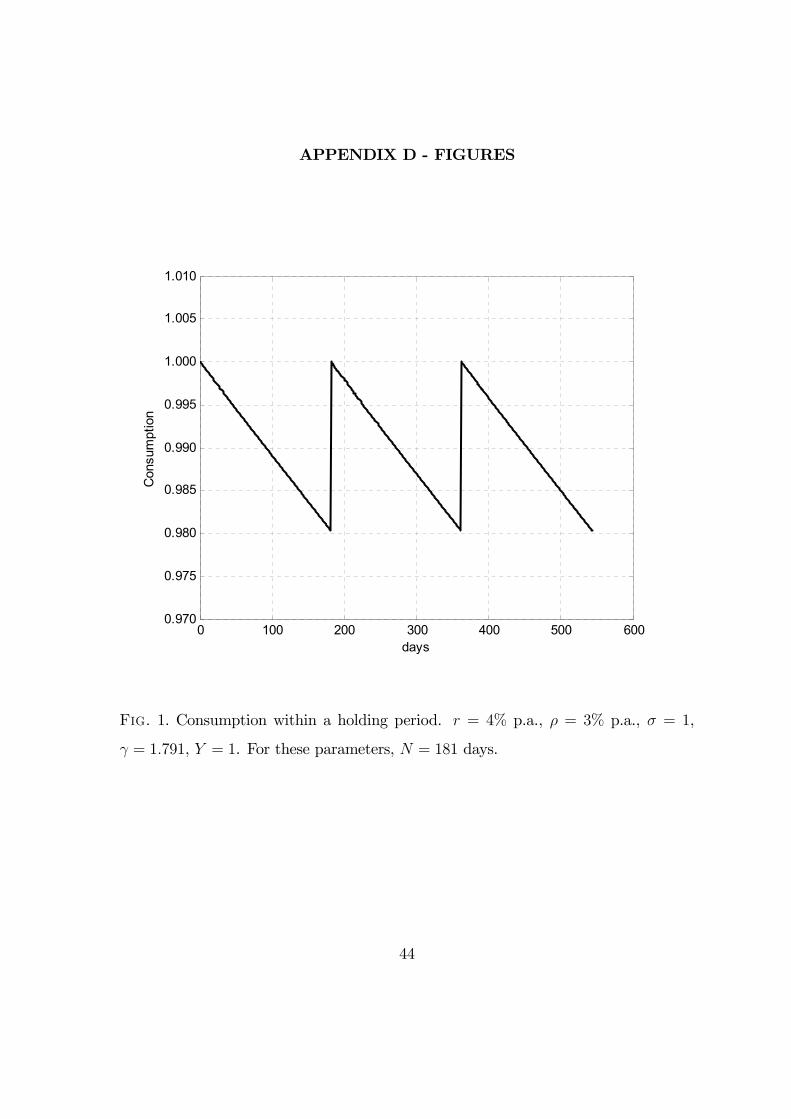
also approximately constant. Figure 1 shows the behavior of consumption within a
holding period for an arbitrary consumer14.
Now we move to the money demand. In the steady state we have a uniform distri-
bution of consumers along the interval [0, N). Index consumers by their position in
this interval, n ∈ [0, N)15. For t > jN , j = 1, 2, ..., consumers with n ∈ [0, t − jN)
will be in their (j + 1)th holding period, and consumers with n ∈ [t− jN,N) will be
in their jth holding period. Aggregate money demand is given by
M (t) =1
N
Z t−jN
0
M (t, n) dn+1
N
Z N
t−jNM (t, n) dn,
where M (t, n) denotes the individual money demand. Solving the integrals above
yields the following proposition.
Proposition 6. In the steady state, the real money demand is given by
m (r, Y, ρ, σ, γ) =c0 (r, Y, ρ, σ, γ)
ρ− r (1− 1/σ)µ1− e−rN/σ
Nr/σ+ e−rN/σ
1− e(r−ρ)N
(r − ρ)N
¶, (17)
where c0 = c0 (r, Y, ρ, σ, γ) is given by Lemma 1 and N = N (r, ρ, σ, γ) is given by
proposition 2.
Proof. See appendix16.
The real money demand is homogeneous of degree one in Y , as c0 is homogeneous
of degree one in Y . Thus, the elasticity of the money demand with respect to income
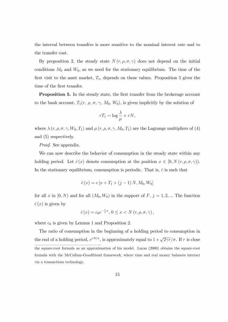
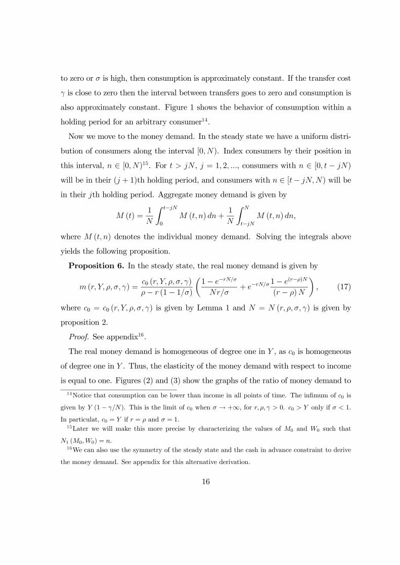
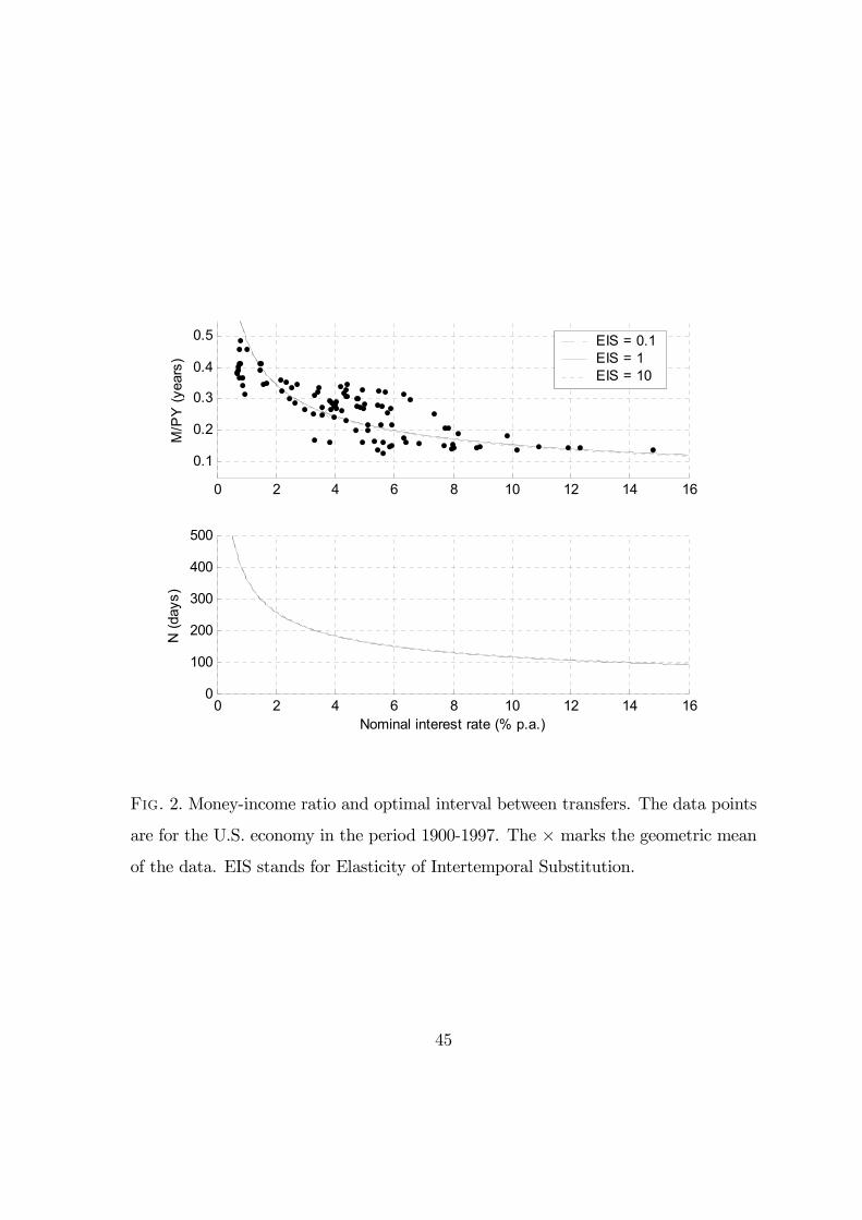
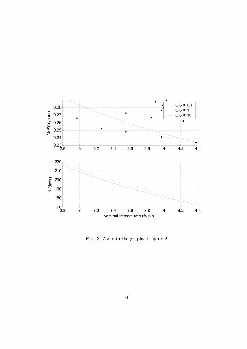
is equal to one. Figures (2) and (3) show the graphs of the ratio of money demand to
14Notice that consumption can be lower than income in all points of time. The infimum of c0 is
given by Y (1− γ/N). This is the limit of c0 when σ → +∞, for r, ρ, γ > 0. c0 > Y only if σ < 1.
In particulat, c0 = Y if r = ρ and σ = 1.15Later we will make this more precise by characterizing the values of M0 and W0 such that
N1 (M0,W0) = n.16We can also use the symmetry of the steady state and the cash in advance constraint to derive
the money demand. See appendix for this alternative derivation.
16
GDP, M/ (PY ), and the equilibrium value of the interval between transfers. Figures
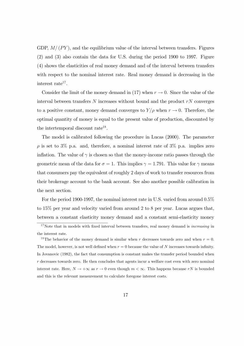
(2) and (3) also contain the data for U.S. during the period 1900 to 1997. Figure
(4) shows the elasticities of real money demand and of the interval between transfers
with respect to the nominal interest rate. Real money demand is decreasing in the
interest rate17.
Consider the limit of the money demand in (17) when r → 0. Since the value of the
interval between transfers N increases without bound and the product rN converges
to a positive constant, money demand converges to Y/ρ when r → 0. Therefore, the
optimal quantity of money is equal to the present value of production, discounted by
the intertemporal discount rate18.
The model is calibrated following the procedure in Lucas (2000). The parameter
ρ is set to 3% p.a. and, therefore, a nominal interest rate of 3% p.a. implies zero
inflation. The value of γ is chosen so that the money-income ratio passes through the
geometric mean of the data for σ = 1. This implies γ = 1.791. This value for γ means
that consumers pay the equivalent of roughly 2 days of work to transfer resources from
their brokerage account to the bank account. See also another possible calibration in
the next section.
For the period 1900-1997, the nominal interest rate in U.S. varied from around 0.5%
to 15% per year and velocity varied from around 2 to 8 per year. Lucas argues that,
between a constant elasticity money demand and a constant semi-elasticity money
17Note that in models with fixed interval between transfers, real money demand is increasing in
the interest rate.18The behavior of the money demand is similar when r decreases towards zero and when r = 0.
The model, however, is not well defined when r = 0 because the value of N increases towards infinity.
In Jovanovic (1982), the fact that consumption is constant makes the transfer period bounded when
r decreases towards zero. He then concludes that agents incur a welfare cost even with zero nominal
interest rate. Here, N → +∞ as r → 0 even though m <∞. This happens because rN is bounded
and this is the relevant measurement to calculate foregone interest costs.
17
demand, the function that best fits the data is a constant elasticity money demand
with elasticity equal to −1/2.According to the graphs in figures (2), (3) and (4) we have the following. (i) The
money demand derived in propositions 2 and 6 is close to the Baumol-Tobin money
demand. This is clear by figure (4) where the numerically-calculated elasticities are
very close to −1/2. (ii) The elasticity of intertemporal substitution has a small effecton the money demand. Three values were used to illustrate this: 0.1, 1 and 10. Only
when we increase the precision of the graph it is possible to distinguish the three
curves. The difference is discernible for the elasticities with respect to the interest
rate, but the differences are small. These calculations were also done for various
values of ρ and the results were similar.
We calculated numerically the elasticities of real money demand and of the interval
N with respect to the transfer cost γ. These values are also around 0.5 for the same
elasticities of intertemporal substitution considered above.
We obtain the equilibrium value of the price level at time zero, P0, with the real
money balances, m, and the initial supply of money, MS0 . It is immediate to verify
that in the steady state inflation is equal to the growth rate of money α and hence
r = ρ + π. Given that the goods and money markets clear, the bonds market also
clears by Walras’ Law.
We now write the values of M0 and W0 that imply a uniform distribution of con-
sumers along the interval [0, N). Let n ∈ [0, N) index consumers by the time ofthe first transfer. Define the functions M0 (n) and W0 (n) respectively as the ini-
tial amounts of deposits in the bank and brokerage accounts such that a consumer³M0 (n) , W0 (n)
´transfers resources at t = n, n + N , n + 2N etc. After the first
withdrawal, the interval between transfers is constant and equal to N .
M0 (n) must be exactly enough to allow the consumer to consume at the steady
state rate in the interval [0, n). On the other hand W0 (n) is equal to the present
18
value of all future transfers from t = n and on, plus the present value of the total
transfer cost. Proposition 7 gives the values of M0 (n) and W0 (n).
Proposition 7. Given the values of N (r, ρ, σ, γ), c0 (r, Y, ρ, σ, γ) and of the price
level at t = 0, P0, the values of the initial money holdings in the bank account, M0 (n),
and of the initial wealth in the brokerage account, W0 (n), such that the consumer
chooses T1 = n are given by
M0 (n) = P0c0erσne−
rσN 1− e−(ρ−r(1−1/σ))n
ρ− r (1− 1/σ)and
W0 (n) =e−ρn
1− e−ρN
µP0c0
1− e−(ρ−r(1−1/σ))N
ρ− r (1− 1/σ) + P0γY
¶,
for n ∈ [0, N (r, ρ, σ, γ)).Proof. See appendix.
M0 (n) is increasing in n while W0 (n) is decreasing in n. A consumer with more
initial money holdings and less initial bond holdings will make the first transfer later
than a consumer with less money and more bonds.
4. WELFARE COST OF INFLATION
When the nominal interest rate is positive, agents deviate real resources from con-
sumption to financial services to maintain the optimal level of money holdings.
The optimal monetary policy is to set the money growth rate at −ρ. In this case,the inflation rate is equal to −ρ and the nominal interest rate is equal to zero. Thisis in accordance to Friedman (1969). But how much does a positive nominal interest
rate cost to society?
The welfare cost of inflation19 is defined as the percentage income compensation
required to leave consumers indifferent between r > 0 and r = 0. Let UT (r, Y ) be
the total welfare, derived from all consumers with equal weight, for an economy with19Or, the “welfare cost of a positive nominal interest rate”.
19
income Y and nominal interest rate r > 0. The welfare cost w (r) is defined as the
solution to
UT [r, (1 + w (r))Y ] = UT (0, Y ) . (18)
In the present model, consumption follows c0e−rt/σ within a holding period for each
agent in the steady state. At each time t we have consumers along the interval [0, N)
in different positions of their holding period. To calculate total utility, we first sum
total utility for each time t and then we sum this value from t = 0 to infinity. This
yields
UT (r, Y ) =1
ρ
1
N
Z N
0
¡c0 (r, Y, ρ, σ, γ;Y ) e
−rt/σ¢1−σ1− σ
dt, (19)
where c0 (r, Y, ρ, σ, γ;Y ) is given by (14). Instead of comparing r > 0 to r = 0, it is
useful to allow a comparison with r > 0. Using (18) and (19) with r > 0 we have the
following proposition.
Proposition 8. The income compensation to leave consumers indifferent between
r > 0 and r > 0 is given by
1 + w (r) =
·³1− γ
N
´ rN/σ
1− e−rN/σ
¸ ·³1− γ
N
´ rN/σ
1− e−rN/σ
¸−1×"rN
rN
1− erN(1−1/σ)
1− erN(1−1/σ)
# 11−σ
,
for σ 6= 1, and
1 + w (r) =
·³1− γ
N
´ rN
1− e−rN
¸ ·³1− γ
N
´ rN
1− e−rN
¸−1× exp
µrN
2− rN
2
¶,
for σ = 1.
Proof. See appendix.
Figure (5) shows the welfare cost for r between zero and 100% p.a. Bringing down
the nominal interest rate from 15% p.a. to 0% p.a yields an increase in welfare
20
equivalent to a permanent increase in income of 2%. Figure (6) shows the welfare
compensation in units that help its interpretation in terms of inflation. The welfare
cost was set to zero for r = 3% p.a., the nominal interest rate compatible with zero
inflation for the U.S. Bringing down inflation from 10% p.a. to 0% p.a. is equivalent
to a permanent increase in income of 1%.
The variable m in the model was interpreted asM1 in the calibration above. With
the transfer cost γ set to 1.791 working days per transfer we have velocity of around
4 per year and an interval between transfers of around six months when r = 4%
p.a. This size for the interval may be viewed as excessive for M1 but it is not for
broader definitions of money. As pointed out by Vissing-Jorgensen (2002) a large
fraction of agents trade assets with higher yields very infrequently, less than once a
year. Moreover, in the data summarized by Alvarez, Atkeson and Edmond (2002), the
opportunity cost in terms of foregone interest is similar for currency, savings deposits
and time deposits (M2 less retail money market mutual funds).
We then reinterpretm according to this broader definition of money and recalibrate
the parameter γ. Alvarez, Atkeson and Edmond find that the opportunity cost of
holding M2 less retail money market is about 200 basic points. Therefore, we set γ
such that velocity equals 1.6 per year when the interest rate is 2% p.a., that is, the
average nominal interest rate of 4% p.a. minus 2% p.a. in opportunity costs. We
obtain γ = 5.9 working days per transfer. This implies an interval between transfers
of around 470 days when the interest rate is 2% p.a. This lower frequency of transfers
is compatible with this broader definition of money. Using this calibration, bringing
down inflation from 10% p.a. to 0% p.a. is equivalent to a permanent increase in
income of 1.75%.
We compare the welfare compensation implied by this model with the one calculated
directly from the Baumol-Tobin money demand. As the interest foregone cancel out
across consumers, the total cost for society is given only by the transfer cost, γY/N .
21
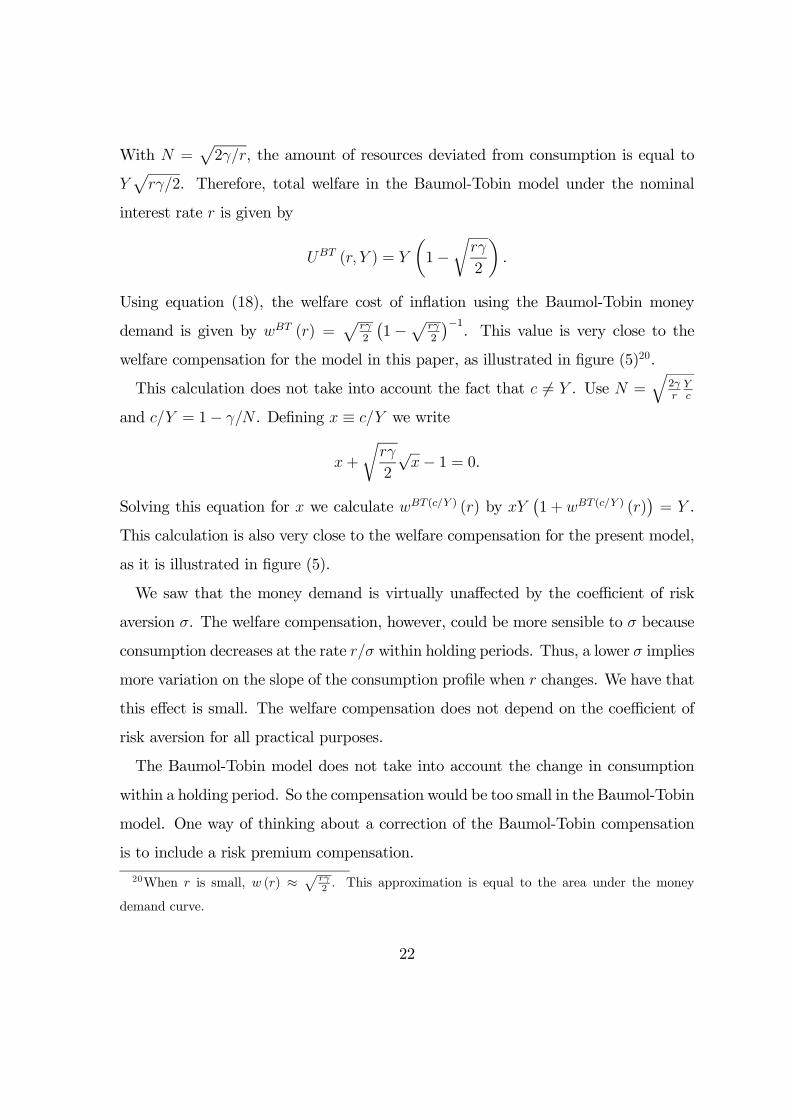
With N =p2γ/r, the amount of resources deviated from consumption is equal to
Yprγ/2. Therefore, total welfare in the Baumol-Tobin model under the nominal
interest rate r is given by
UBT (r, Y ) = Y
µ1−
rrγ
2
¶.
Using equation (18), the welfare cost of inflation using the Baumol-Tobin money
demand is given by wBT (r) =p
rγ2
¡1−prγ
2
¢−1. This value is very close to the
welfare compensation for the model in this paper, as illustrated in figure (5)20.
This calculation does not take into account the fact that c 6= Y . Use N =q
2γrYc
and c/Y = 1− γ/N . Defining x ≡ c/Y we write
x+
rrγ
2
√x− 1 = 0.
Solving this equation for x we calculate wBT (c/Y ) (r) by xY¡1 + wBT (c/Y ) (r)
¢= Y .
This calculation is also very close to the welfare compensation for the present model,
as it is illustrated in figure (5).
We saw that the money demand is virtually unaffected by the coefficient of risk
aversion σ. The welfare compensation, however, could be more sensible to σ because
consumption decreases at the rate r/σ within holding periods. Thus, a lower σ implies
more variation on the slope of the consumption profile when r changes. We have that
this effect is small. The welfare compensation does not depend on the coefficient of
risk aversion for all practical purposes.
The Baumol-Tobin model does not take into account the change in consumption
within a holding period. So the compensation would be too small in the Baumol-Tobin
model. One way of thinking about a correction of the Baumol-Tobin compensation
is to include a risk premium compensation.
20When r is small, w (r) ≈ prγ2 . This approximation is equal to the area under the money
demand curve.
22
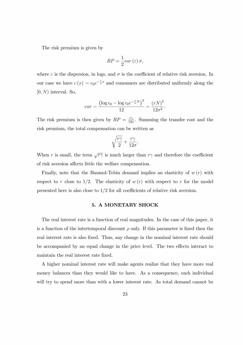
The risk premium is given by
RP =1
2var (ε)σ,
where ε is the dispersion, in logs, and σ is the coefficient of relative risk aversion. In
our case we have c (x) = c0e− rσx and consumers are distributed uniformly along the
[0, N) interval. So,
var =
¡log c0 − log c0e− r
σN¢2
12=(rN)2
12σ2.
The risk premium is then given by RP = rγ12σ. Summing the transfer cost and the
risk premium, the total compensation can be written asrrγ
2+
rγ
12σ.
When r is small, the term√rγ is much larger than rγ and therefore the coefficient
of risk aversion affects little the welfare compensation.
Finally, note that the Baumol-Tobin demand implies an elasticity of w (r) with
respect to r close to 1/2. The elasticity of w (r) with respect to r for the model
presented here is also close to 1/2 for all coefficients of relative risk aversion.
5. A MONETARY SHOCK
The real interest rate is a function of real magnitudes. In the case of this paper, it
is a function of the intertemporal discount ρ only. If this parameter is fixed then the
real interest rate is also fixed. Thus, any change in the nominal interest rate should
be accompanied by an equal change in the price level. The two effects interact to
maintain the real interest rate fixed.
A higher nominal interest rate will make agents realize that they have more real
money balances than they would like to have. As a consequence, each individual
will try to spend more than with a lower interest rate. As total demand cannot be
23
higher than total output, and output is constant, the price level increases. The price
change will curb any upward movement in demand. This explanation for the increase
in prices can be found, for example, in Friedman (1969)21.
Therefore, eventually the price level will adapt to the new interest rate. Nothing
indicates, however, how fast the price level will reach its new path. In the present
model, the transfer cost makes agents economize the use of money. In order to avoid
making a transfer too soon, agents will not increase their consumption as they would
without the transfer cost. Consequently, prices do not change instantaneously with
the change in the nominal interest rate.
This behavior can be seen in figure (7). It contains the price in logs after an increase
in the nominal interest rate of one percentage point. The initial nominal interest rate
is equal to the discount parameter ρ = 3% p.a. Hence, this change implies a 1% p.a.
inflation rate in the new steady state from an economy with zero inflation.
According to the simulation results displayed in figure (7), the price level drops
at the moment of the shock. Moreover, the inflation rate is initially lower than its
steady state value of 1% p.a.
After about six months, however, two groups of consumers with different consump-
tion patterns meet. The first group is composed of those who had substantial money
holdings at time zero and have not made a transfer after the shock. The second group
is formed by the consumers who have already made a transfer and are now doing their
second transfer. When the two groups meet there is a fast increase in the price level,
otherwise, demand would be much higher because the second group consumes at a
faster rate. After the nominal interest rate shock, therefore, the model predicts an
initial price drop, followed by relatively low inflation, and an inflation overshooting
21Friedman studies a permanent increase in the individual money holdings, not an increase in the
nominal interest rate. But in both cases agents have more real balances than they would like to
have.
24
after six months. The effects of the change in the nominal interest rate can be felt
long after the shock.
The price level does not adjust instantaneously to the interest rate shock. This
addresses the apparent price stickiness after a change in the nominal interest rate
reported, for example, in Christiano, Eichenbaum and Evans (1999).
Grossman and Weiss (1983) and Rotemberg (1984) study the effects of monetary
shocks in economies where agents transfer funds periodically. A more recent model
with this feature is Alvarez, Atkeson and Edmond (2002). In these models, the
interval between transfers is exogenously set22.
We now define the structure to study a nominal interest shock. We want to ap-
proximate a situation in which the economy is initially in the steady state and the
interest rate changes unexpectedly. The money holdings at the time of the shock are
equal to the values compatible with the economy in the steady state.
Suppose the existence of two possible states denoted by s = 1, 2. In state 1 the
government sets the nominal interest rate at r1 for all periods. In state 2, the nominal
interest rate is set at r2. The realization of the state occurs at time zero.
Agents trade bonds contingent on the realization of the states. Denote by θ the
probability of the state being equal to 1. Trade occurs through the brokerage account.
Only deposits in the brokerage account change according to the state. Money holdings
are not state contingent.
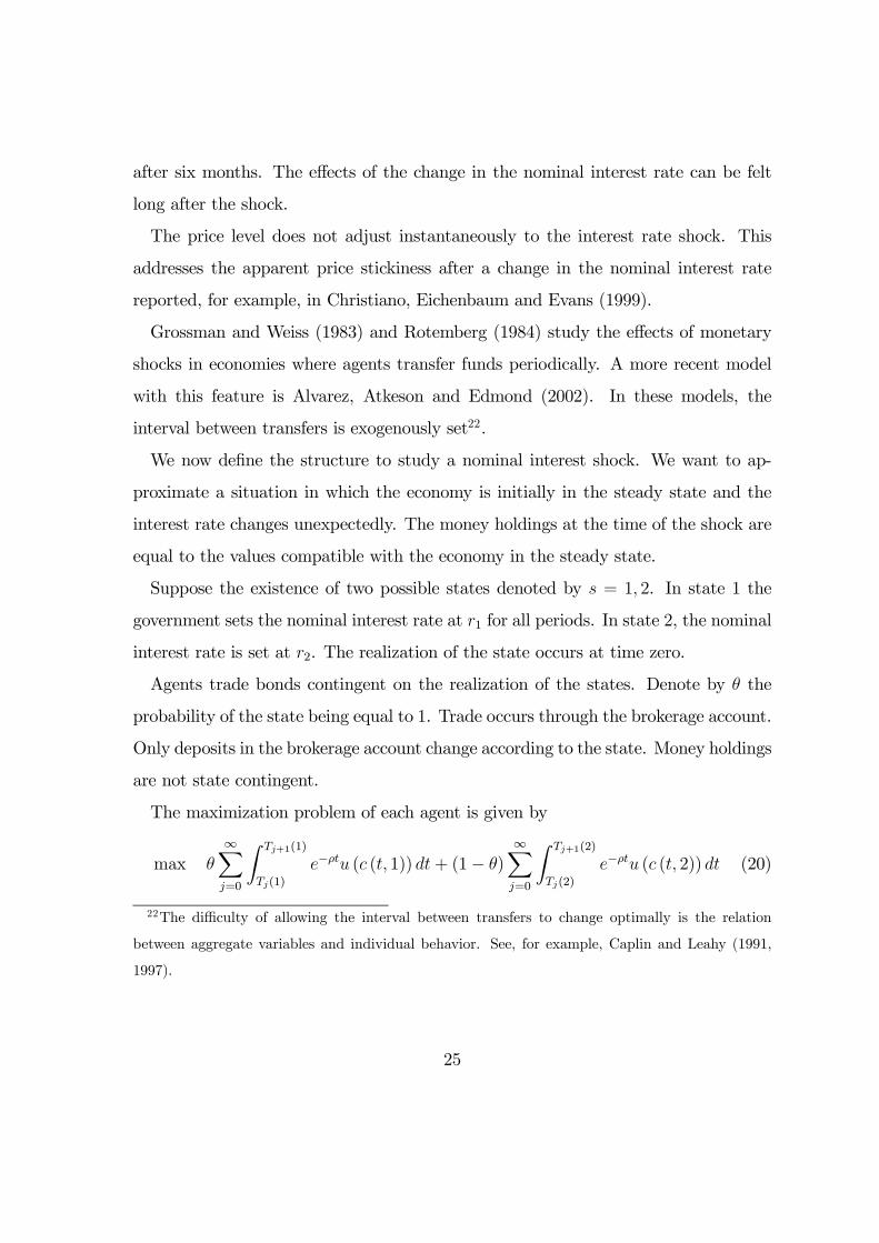
The maximization problem of each agent is given by
max θ∞Xj=0
Z Tj+1(1)
Tj(1)
e−ρtu (c (t, 1)) dt+ (1− θ)∞Xj=0
Z Tj+1(2)
Tj(2)
e−ρtu (c (t, 2)) dt (20)
22The difficulty of allowing the interval between transfers to change optimally is the relation
between aggregate variables and individual behavior. See, for example, Caplin and Leahy (1991,
1997).
25
subject to
Xs=1,2
" ∞Xj=1
Q (Tj (s) , s)
Z Tj+1(s)
Tj(s)
P (t, s) c (t, s) dt
+∞Xj=1
Q (Tj (s) , s)P (Tj (s) , s) γY
#=W0 +
Xs=1,2
Q (T1 (s) , s)K (s) , (21)
Z T1(1)
0
P (t, 1) c (t, 1) dt+K (1) =M0, (22)Z T1(2)
0
P (t, 2) c (t, 2) dt+K (2) =M0. (23)
Where W0 denotes deposits in the brokerage account,
W0 ≡ B0 +Xs=1,2
Z ∞
0
Q (t, s)P (t, s)Y dt.
Agents differ by their money and bond holdings M0 and W0.
Note that we have a single budget constraint after the first transfer. Agents are
able to trade bonds using the resources of the brokerage account. But their money
holdings do not change with the state.
In section 3, we start from an economy with constant nominal interest rate and we
move backwards to find a distribution ofM0 andW0 over consumers. This distribution
is such that the economy is in equilibrium since time zero and hence it is in fact
compatible with a constant nominal interest rate.
Following the same reasoning, we seek a distribution of M0 and W0 such that the
economy is in equilibrium after the realization of the state. The difference is that
now the price level will not increase at a constant inflation rate as in the stationary
equilibrium. For either state 1 or state 2, the inflation rate will not be constant.
The task of find M0 and W0 for each agent is facilitated if we assume that the
probability θ is arbitrarily close to one. In this case, M0 and W0 are very close to the
values such that the economy is under state one without the possibility of starting
26
in state two. These are the amounts of money and bonds calculated in section 3.
Moreover, the Lagrange multiplier associated to the present value budget constraint
(21), denoted by λ, is the same as if the economy had only state 1 as the possible
starting state. Recall that λ is the same across agents in the steady state.
To summarize, we first calculate the money holdings and bond holdings such that
the economy is in the steady state under the nominal interest rate r1. With this,
we calculate the value of λ associated to this state. We then calculate individual
consumption using the first order conditions of the maximization given above, with
the value of M0 for each agent and the value of λ.
In the steady state, agents can be distributed over the interval [0, N), where the
interval between transfers N is given by the parameters ρ, σ and γ, and the nominal
interest rate r. The values of M0 and W0 are then given by M0 (n) and W0 (n), for
n ∈ [0, N), stated in proposition 7.The individual consumption depends on the price level P (t). We need to find, for
each agent, the optimal consumption and the optimal timing of a transfer. We have
these values by the two following propositions23.
Proposition 9. The timing of a transfer Tj (n) of consumer n ∈ [0, N) is given by
− e(1−1/σ)r2Nj(n) − 11− 1/σ +
γY [r2 − π (Tj (n))]
c+ (Tj (n))
= −r2 eρTj(n)/σ
P (Tj (n))1−1/σ
Z Tj+1(n)
Tj(n)
e−ρt/σP (t)1−1/σ dt,
where c+ (Tj (n)) =£λeρTj(n)Q (Tj (n))P (Tj (n))
¤−1/σand j = 2, 3, ... The consump-
tion level c (t, n) of agent n at time t is given by
c (t, n) =
·e−ρt
λQ (Tj)P (t)
¸1/σ, t ∈ (Tj (n) , Tj+1 (n)) , j = 1, 2, ...
23Recall that Q (t) = e−rt and that Tj (n) ≡ N1 + ... + Nj . We also have that λ = 1P0cσ0
, where
P0 is the price level in the initial steady state (before the shock) and c0 is the level of consumption
just after a transfer in the initial steady state. See section 3 for notation.
27

For the logarithmic case, σ = 1, the values of Tj (n), j = 2, 3, ..., are given by
−r2Nj (n) +γY [r2 − π (Tj (n))]
c+ (Tj (n))= −r21− e−ρNj+1(n)
ρ.
Proof. See appendix.
Proposition 10. The first transfer T1 (n) of consumer n ∈ [0, N) is given by"µµ (n)
λ
¶1−1/σe(1−1/σ)r2T1(n) − 1
#σ
1− σ+
γY [r2 − π (T1 (n))]
c+ (T1 (n))
− r2K (n)
P (T1 (n)) c+ (T1 (n))= −r2 eρT1(n)/σ
P (T1 (n))1−1/σ
Z T2(n)
T1(n)
eρt/σP (t)1−1/σ dt,
for σ 6= 1, and
−r2T1 − log µ (n)λ
+γY [r2 − π (T1 (n))]
c+ (T1 (n))− r2K (n)
P (T1 (n)) c+ (T1 (n))= −r21− e−ρN2
ρ,
for σ = 1. µ (n) is the Lagrange multiplier associated to the budget constraints (22)
and (23).
Proof. See appendix.
We proceed numerically in order to obtain the values of the timing of the transfers
and consumption. We assume that after the Jth transfer each consumer chooses
NJ+1 = N 0, where N 0 is the interval between transfers under the new nominal interest
rate r2. We also start with a guess of the price level P (t).
Therefore, propositions 9 and 10 imply a system of J equations and J unknowns
given by the intervals N1, ..., NJ . Once we determine the values of the Nj’s, we also
obtain the consumption levels of each agent.
We discretize the interval [0, N) to {n1, n2, ..., nmax} where n1 = 0 and nmax < N .
For each time t we must have, in equilibrium,
1
nmax
Xn
c (t, n) +1
nmaxγY ×Number of Transfers (t) = Y . (24)
The left hand side of this equation is equal to aggregate demand. Their components
are consumption and resources used to transfer assets from the brokerage account to
the bank account. The right hand side is equal to aggregate supply.
28
If the equilibrium condition in (24) is not satisfied, we change the price level at
time t and recalculate the consumption levels and transfer times. We continue to do
this until the difference between demand and supply is smaller than a preestablished
value for every t. If demand is higher than supply, we increase the price level at t. If
demand is lower than supply, we decrease the price level.
The results reported in this paper are for the simulations with J = 40 and a number
of consumers such that the difference ni+1 − ni is given by 0.20 days. This implies
1, 047 consumers for the parameters used. In particular, we assume utility to be
logarithmic and γ = 1.791. The nominal interest rate increases from 3% to 4% p.a.
The number of transfers at t is calculated summing the agents with Tj (n) such that
t ≤ Tj (n) < t + 1. The maximum difference between demand and supply after the
last iteration is given by 2.2% for a total of 150 iterations24,25.
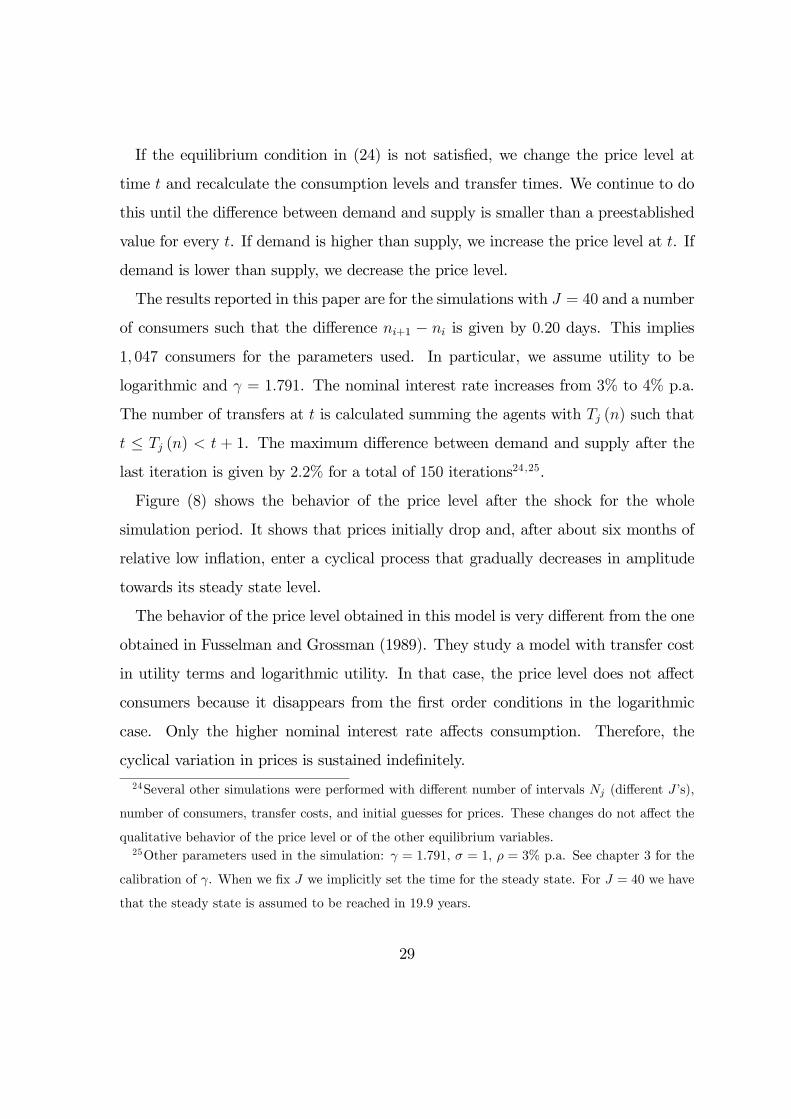
Figure (8) shows the behavior of the price level after the shock for the whole
simulation period. It shows that prices initially drop and, after about six months of
relative low inflation, enter a cyclical process that gradually decreases in amplitude
towards its steady state level.
The behavior of the price level obtained in this model is very different from the one
obtained in Fusselman and Grossman (1989). They study a model with transfer cost
in utility terms and logarithmic utility. In that case, the price level does not affect
consumers because it disappears from the first order conditions in the logarithmic
case. Only the higher nominal interest rate affects consumption. Therefore, the
cyclical variation in prices is sustained indefinitely.
24Several other simulations were performed with different number of intervals Nj (different J ’s),
number of consumers, transfer costs, and initial guesses for prices. These changes do not affect the
qualitative behavior of the price level or of the other equilibrium variables.25Other parameters used in the simulation: γ = 1.791, σ = 1, ρ = 3% p.a. See chapter 3 for the
calibration of γ. When we fix J we implicitly set the time for the steady state. For J = 40 we have
that the steady state is assumed to be reached in 19.9 years.
29
What is making prices to smooth gradually in the present model is the change
in behavior caused by the variation of prices. If prices are unusually high during a
certain period, agents avoid making a transfer because they will pay a higher transfer
cost. This redistributes consumers in a way that the number of transfers does not
continue indefinitely to be concentrated over some intervals. This redistribution is
slow, even five years after the shock the economy still experiences strong variation in
the price level.
The rate of inflation after the shock implied by the price series is in figures (9) and
(10)26. The shock to the interest rate causes a strong variation in the inflation rate.
Gradually, the peaks and troughs of the inflation rate converge towards its steady
state level of 1% p.a.
Figures (11) and (12) show respectively the nominal demand and the money-income
ratio after the shock. In the second steady state, the nominal money demand increases
at the steady state rate of inflation, 1% p.a. According to the simulations, we find
that the nominal money demand decreases about 13% during the first 6 months after
the shock. We have then a long period of money demand cycles with high amplitude.
The cycles of the nominal money demand seem to converge in around 14 years after
the shock, after all consumers made about 28 transfers. We still find, however, a new
series of cycles, with smaller amplitude after this period27.
The money-income ratio or, equivalently, the real money demand, has a similar
behavior as observed in figure (12). Note that the real money demand must eventually
decrease with a higher nominal interest rate. According to the simulations, the real
money demand decreases around 12% in the first six months. A little less than the
26In order to filter the variation of the price level caused by the numerical simulation, the price
series in this figure was filtered for the calculation of inflation. It was used the Hodrick-Prescott
filter. Since the original series is in days, the parameter λ was set to 400× 365.27It is possible that these new cycles are caused by the numerical procedure, magnified by the
continuous increase in the money demand of 1% p.a.
30
15% decrease predicted by the −1/2 elasticity after the 1 percentage point increase inthe nominal interest rate28. After that, the real money demand shows cycles of high
amplitude for a long period, but apparently converge to a lower value, with cycles of
smaller amplitude29.
6. CONCLUSION
We present a Baumol-Tobin model in general equilibrium to measure the welfare
cost of inflation and to calculate the effects on prices after an interest rate shock.
Spending is constant in Baumol and Tobin. But even when agents exhibit high
elasticity of intertemporal substitution and consumption varies considerably within
holding periods, the optimal choice of the interval and the aggregate money demand
are close to the ones in Baumol and Tobin.
The monetary policy that maximizes welfare is to decrease money supply at the
rate of intertemporal discounting, ρ. This sets the nominal interest rate to zero.
When the nominal interest rate decreases towards zero, money demand increases to
the present value of output, Y/ρ.
The welfare cost calculations could differ substantially according to the intertem-
poral elasticity. But the calculations yield that consumers are affected in the same
way by inflation in the steady state, independently of their elasticity of intertemporal
substitution.
The source of welfare loss caused by inflation in this model is the deviation of
resources from consumption to the management of money holdings. But other sources
28Since the beginning interest rate is equal to 3%. An increase to 4% is a 33% increase in the
nominal interest rate. The real money demand decreases 13% after 194 days, the lowest point in
the first year.29As for the nominal money demand, it is possible that these new cycles are caused by the
numerical procedure.
31
of welfare loss may be more important, specially for high inflation rates. One of them
is the difficulty in obtaining information through the price mechanism, as pointed out
by Harberger (1998).
The model is suitable to study the effects of a change in the nominal interest rate
when agents decide the moment to exchange bonds for money. The adjustment to
the new steady state involves a slow increase in the inflation rate, as opposed to the
instantaneous adjustment found in most models. The convergence to the new steady
state is slow. According to the simulations with the calibrated model, inflation varies
high above and below its steady state level after 5 years after the shock. The path of
prices and consumption during the transition leads to the study of the gain in welfare
of a price stabilization program.
APPENDIX A - FIRST ORDER CONDITIONS
The Lagrangian of the problem in (1), (4) and (5) is
L =∞Xj=0
Z Tj+1
Tj
e−ρtu (c (t)) dt+ λ (M0,W0)
W0 +Q (T1)K (M0,W0)
−∞Xj=1
Q (Tj)
Z Tj+1
Tj
c (t,M0,W0)P (t) dt−∞Xj=1
Q (Tj)P (Tj)Y γ]
#
+µ (M0,W0)
·M0 −
Z T1
0
P (t) c (t,M0,W0) dt−K (M0,W0)
¸where we use the fact thatM+ (Tj) =
R Tj+1Tj
P (t) c (t,M0,W0) dt and Tj = Tj (M0,W0).
The first order conditions are given by the equations below.
c (t,M0,W0) :
e−ρtu0 (c (t,M0,W0)) = λ (M0,W0)Q (Tj)P (t) , t ∈ (Tj, Tj+1) ,e−ρTju0
¡c+ (Tj,M0,W0)
¢= λ (M0,W0)Q (Tj)P (Tj) ,
e−ρTj+1u0¡c− (Tj+1,M0,W0)
¢= λ (M0,W0)Q (Tj)P (Tj+1) ,
32
for j = 1, 2, ...;
e−ρtu0 (c (t,M0,W0)) = µ (M0,W0)P (t) , t ∈ (0, T1) ,u0¡c+ (0,M0,W0)
¢= µ (M0,W0)P (0) ,
e−ρT1u0¡c− (T1,M0,W0)
¢= µ (M0,W0)P (T1) .
T1 :
e−ρT1u¡c− (T1)
¢− e−ρT1u¡c+ (T1)
¢= λ
·−Q (T1)K + Q (T1)
Z T2
T1
c (t)P (t) dt−Q (T1) c+ (T1)P (T1) dt
¸+λY γ
hQ (T1)P (T1) +Q (T1) P (T1)
i+µP (T1) c
− (T1) ;
Tj, j = 1, 2, ... :
e−ρTju¡c− (Tj)
¢− e−ρTju¡c+ (Tj)
¢= λ
"Q (Tj)
Z Tj+1
Tj
c (t)P (t) dt
−Q (Tj) c+ (Tj)P (Tj) +Q (Tj−1) c− (Tj)P (Tj)¤
+ λγYhQ (Tj)P (Tj) +Q (Tj) P (Tj)
i.
K :
Q (T1)λ (M0,W0)− µ (W0,M0) ≤ 0 ( = 0 if K > 0);
and the budget constraints.
With CRRA utility, u0 (c (t)) c (t) = (1− σ)u (c (t)) for σ 6= 1. Using this in the
first order condition for Tj, j = 2, 3, ..., we have, after simplification
γY [r (Tj)− π (Tj)] +1
1− σ
·Q (Tj−1)Q (Tj)
c− (Tj)− c+ (Tj)
¸=
·Q (Tj−1)Q (Tj)
c− (Tj)− c+ (Tj)
¸− r (Tj)
Z Tj+1
Tj
P (t) c (t)
P (Tj)dt.
33
If σ = 1, we obtain
γY [r (Tj)− π (Tj)] + c+ (Tj) logQ (Tj)
Q (Tj−1)= −r (Tj)
Z Tj+1
Tj
c (t)P (t)
P (Tj)dt.
Using the budget constraint and the first order condition with respect to consump-
tion, the value of λ (M0,W0) is given by
λ (M0,W0) =∞Xj=1
Z Tj+1
Tj
e−ρt [c (t)]1−σ dt
×"W0 +Q (T1)K − γY
∞Xj=1
Q (Tj)P (Tj)
#−1for σ 6= 1, and
λ (M0,W0) =e−ρT1
ρ
"W0 +Q (T1)K − γY
∞Xj=1
Q (Tj)P (Tj)
#−1(25)
for σ = 1. Working analogously for µ (M0,W0) using the budget constraint for 0 ≤t < T1, we obtain
µ (M0,W0) =1
M0 −K
·Z T1
0
e−ρt [c (t)]1−σ dt¸
(26)
for σ 6= 1, andµ (M0,W0) =
1
M0 −K
1− e−ρT1
ρ
for σ = 1.
APPENDIX B - PROOFS
Proposition 1
Proof. Consider the solution c (t,M0,W0;Y ), K (M0,W0;Y ), and Nj (M0,W0;Y )
of a consumer with (M0,W0, Y ). Multiply (M0,W0, Y ) by h > 0. The values
hc (t,M0,W0;Y ), hK (t,M0,W0;Y ), and Tj (M0,W0;Y ) satisfy the budget constraint
of the new problem. By the equations for the Lagrange multipliers, we see that
34
λ (W0,M0;Y ) and µ (W0,M0;Y ) are homogeneous of degree (−σ) in (W0,M0, Y ).
Hence, hc (t,M0,W0;Y ), hK (t,M0,W0;Y ), and Tj (M0,W0;Y ) satisfy the first or-
der conditions for consumption, for Tj and for K. For money holdings, we have
M+ (Tj, hM0, hW0;hY ) = hM+ (Tj,M0,W0;Y ) using
M+ (Tj,M0,W0;Y ) =
Z Tj+1
Tj
P (t) c (t,M0,W0;Y ) dt.¥
Lemma 1
Proof. Consumption within a holding period is given by c (t) = c0e− rσ(t−Tj), Tj ≤
t < Tj+1 using its first order condition. In the steady state, total consumption at
each time t is given by
1
N (r, ρ, σ, γ)
Z N(r,ρ,σ,γ)
0
c0e− rσxdx.
Hence the market clearing condition in the steady state implies
1− e−rσN(r,ρ,σ,γ)
rN (r, ρ, σ, γ) /σc0 +
γY
N (r, ρ, σ, γ)= Y
⇒ c0 = Y
µ1− γ
N (r, ρ, σ, γ)
¶rN (r, ρ, σ, γ) /σ
1− e−rN(r,ρ,σ,γ)/σ.¥
Proposition 2
Proof. The first order condition with respect to Tj in the steady state implies, after
simplification,
− σ
1− σ
£c+ (Tj)− c− (Tj) erNj
¤= −r
Z Tj+1
Tj
c (t)P (t)
P0eπTjdt+ γY (r + π) .
Using c (t) = c0e− rσ(t−Tj), j = 1, 2, ..., r = ρ+ π, and simplifying, yields
− 1
1− 1/σ£1− erNj(1−1/σ)¤− ργ
Y
c0= r
1− e−ρNj+1erNj+1(1−1/σ)
ρ− r (1− 1/σ) .
With Nj = Nj+1 = N we have the desired result. The steps for σ = 1 are analogous.
Note also that
limσ→1− 1
1− 1/σ£1− erN(1−1/σ)
¤= rN .¥
35
Proposition 3
Proof. Define the functions a, b,G : (γ,+∞)→ R for σ 6= 1 by
a (N) =
µ1− e−rN/σ
rN/σ
¶³1− γ
N
´−1,
b (N) =σ
1− σ
¡1− e−rN(1−σ)/σ
¢− r1− e−rN(1−σ)/σe−ρN
ρ+ r (1− σ) /σ,
and
G (N) = b (N)− ργa (N) .
Note that a = Y/c0. The optimal interval N∗ is such that G (N∗) = 0.
We have limN→γ+ a (N) = +∞ and limN→γ+ b (N) = 0. Therefore,
limN→γ+
G (N) = −∞.
We also have that limN→∞ a (N) = 0. Intuitively, if N →∞ then the consumer is
consuming almost his total present value in the beginning of the holding period. So
c0 is very large, and a = Y/c0 → 0. Moreover, b0 (N) > 0, and a0 (N) < 0 because
erN/σ > 1 +Nr/σ − γr/σ. Hence,
G0 (N) = b0 (N)− ργa0 (N) > 0.
Even though G is always increasing, it can be the case that limN→+∞G (N) < 0.
This possibility is ruled out for σ ≥ 1 because limN→∞ b0 (N) = +∞ for σ > 1 and
limN→∞ b0 (N) = r for σ = 1. On the other hand, limN→∞ b0 (N) = 0 for 0 < σ < 1.
In this case, limN→+∞G (N) = limN→+∞ b (N) = σρ > 0.¥Proposition 4
Proof.
(i) ∂N/∂r = − (∂G/∂r) /G0 (N). We know that G0 (N) > 0. On the other hand,
∂b (N, r)
∂r= Ne−rN(1−σ)/σ
µ1− r (1− σ) /σe−ρN
ρ+ r (1− σ) /σ
¶> 0
36
and∂a (N, r)
∂r=
µ(1 + rN/σ)− erN/σ
erN/σr2 (N/σ)
¶³1− γ
N
´−1< 0.
Therefore, ∂G/∂r = ∂b (N) /∂r − ργ∂a (N) /∂r > 0 and then ∂N/∂r < 0.
(ii) ∂G/∂γ = −ρa (N)−ργ∂a (N) /∂γ, ∂a (N) /∂γ =³1−e−rN/σrN/σ
´N
(N−γ)2 > 0. Thus,
∂G/∂γ < 0 and ∂N/∂γ = − (∂G/∂γ) /G0 (N) > 0.
(iii) For σ = 1,
ρ∂G
∂ρ=
r
ρ
¡1− e−ρN
¢− rNe−Nρ − ργ
µ1− e−rN
rN
¶³1− γ
N
´−1.
Use the value of the third term in the left hand side implied by G (N∗) = 0 to obtain
ρGρ = 2r
ρ
¡1− e−ρN
¢− rN¡1 + e−ρN
¢.
Then, Gρ < 0⇐⇒ −2¡1− e−ρN
¢+ ρN
¡1 + e−ρN
¢> 0. Define
f (x) = −2 ¡1− e−x¢+ x
¡1 + e−x
¢.
We have f (0) = 0 and f 0 (x) = 1− e−x (1 + x) > 0. Therefore, Gρ < 0 and ∂N/∂ρ =
−Gρ/G0 (N) > 0. As G (σ,N) is continuous in σ, we also have ∂N/∂ρ > 0 for σ
sufficiently close to 1. Moreover, numerical simulations yield that ∂N/∂ρ > 0 for any
σ > 0.
(iv) The optimal N is given by G (N) = 0. As G is increasing and continuous in
N , and limN→γ+ G (N) = −∞ then it must be the case that the optimal N is higher
than γ.
(v) We saw that N decreases when γ decreases and that N > γ. The equation that
determines N converges to
− 1
1− 1/σ¡1− erN(1−1/σ)
¢= r
1− e−N(ρ−r(1−1/σ))
ρ− r (1− 1/σ)when γ → 0. This expression holds if and only if N = 0.
37
(vi) When r decreases, N increases. But limr→0 rN is bounded because |∂N/∂r| <1. Define x ≡ limr→0 rN . Using the equation that defines N and limr→0N = +∞,the value of x is given by
− 1
1− 1/σ¡1− ex(1−1/σ)
¢= ργ
µ1− e−x/σ
x/σ
¶.
In order to have an idea of the magnitude of this number, consider this equation for
σ = 1,
x = ργ
µ1− e−x
x
¶.
This value of x is approximately equal to ργ/ (1 + ργ/2).¥Proposition 5
Proof. By the first order condition for T1 and e−ρtu (c) = cµ (M0,W0)P (t) / (1− σ).
We obtain, after rearranging,
σ
1− σ
µ
Q (T1)c− (T1)− σ
1− σλc+ (T1)
= λ
"−Q (T1)Q (T1)
K
P (T1)
Q (T1)
Q (T1)
Z T2
T1
c (t)P (t)
P (T1)dt
#+ λY γ
"Q (T1)
Q (T1)+
P (T1)
P (T1)
#.
In the steady state, we know that c (t) = c0e− rσ(T2−t), T1 ≤ t < T2, c− (T1) = c0e
− rσN ,
and c+ (T1) = c0. Also, inflation is constant and r = ρ + π. Then, with K = 0 and
after simplification
σ
1− σerT1e−
rσN − σ
1− σ
λ
µ=
λ
µ
·−r1− e−(ρ−r(σ−1)/σ)N
ρ− r (σ − 1) /σ − ρY
c0γ
¸.
With the optimality condition for N , we obtain
erT1e−rσN =
λ
µe−
rσNerN .
Taking logs on both sides yields the desired result.¥Proposition 6
Proof. We provide two proofs for this proposition.
38
(1) For t > jN , consumers will be in their jth or (j + 1)th holding period, j =
1, 2, ... Individual money demand is given by
M (t, n) =
R Tj+2(n)t
P (t) c0e− rσ(t−Tj+1(n))dt, n ∈ [0, t− jN),R Tj+1(n)
tP (t) c0e
− rσ(t−Tj(n))dt, n ∈ [t− jN,N).
where Tj (n) ≡ n + (j − 1)N . Solving the integrals and with a change of variables,aggregate money demand is given by
M (t) =1
N
Z t
t−NP0c0
eπ(s+N)e−rN/σ − eπte−r(t−s)/σ
(π − r/σ)ds
or,M (t)
P (t)=
c0N
Z N
0
e(r−ρ−r/σ)Ne−(r−ρ)x − e−rx/σ
(r − ρ− r/σ)dx.
Solving the integral, with the value of c0 given by Lemma 1 and withm ≡M (t) /P (t),
we obtain the real money demand in the text.¥(2) Real money demand for any consumer in the stationary equilibrium is such that
mn (t) = −cn (t)− πmn (t) ,
where m denotes real money demand and the superscript refers to the consumer
with n ∈ [0, N). For n = 0, the boundary condition for this differential equation ism (N) = 0. Solving the differential equation, we obtain
m0 (t) = c0e−rt e
ρ(t−N)er(1−1/σ)N − er(1−1/σ)t
r (1− 1/σ)− ρ.
By the symmetry of the steady state, aggregate real money demand is given by
m (t) =1
N (r, ρ, σ, γ)
Z N(r,ρ,σ,γ)
0
m0 (t) dt.
Substituting m0 (t) and solving the integral yields the desired result.¥Proposition 7
39
Proof. M0 (n) is exactly enough to allow the consumer to consume at the steady
state rate in the interval [0, n). This value is such that
M (n) =
Z n
0
P (t) c (t) dt.
c (0) is not necessarily equal to the level of consumption when a transfer is made.
This is only true for the consumer n = 0. We know that
c− (n) = c0e− rσN ,
for all n ∈ [0, N), and thatc
c= − r
σ.
Solving this differential equation yields
c (x, n) = c0erσne−
rσNe−
rσx, 0 ≤ x < n.
Therefore, solving the integral
M (n) =
Z n
0
P0eπtc0e
rσne−
rσNe−
rσtdt
we have the desired result for M (n) .
For W0 (n). First, the value of money needed in each holding period is given by
Mj =
Z n+jN
n+(j−1)NP (t) c0e
− rσ(t−Tj)dt,
where j = 1, 2, ... and Tj = n+ (j − 1)N . So,
Mj = P0c0eπn e
(π−r/σ)N − 1(π − r/σ)
eπ(j−1)N ≡ Meπ(j−1)N
The value at t = n of these transfers is AM ≡ M 11−e−ρN . For the transfer cost, we
have
TCj = γY P (n+ (j − 1)N) , j = 1, 2, ...= P0γY e
π(n+(j−1)N).
40
Working analogously, ATC ≡ P0γY eπn 11−e−ρN . Finally, the value of W (n) is given by
W (n) = e−rnAM + e−rnATC.¥
Proposition 8
Proof. Substitute the value of c0 given by equation (14) in the integral in the text.
Use this calculation in equation (18) to obtain the desired result. For σ = 1, follow
the same steps with u (c) = log c.¥Proposition 9
Proof. From the first order conditions of the utility maximization problem with
respect to c (t) and Tj we have
c+ (Tj)
·Q (Tj−1)Q (Tj)
c− (Tj)c+ (Tj)
− 1¸
σ
1− σ+ γY [r2 − π (Tj)] = −r2
Z Tj+1
Tj
P (t) c (t)
P (Tj)dt.
Where we used the fact that³c+(Tj)
c−(Tj)
´−σ=
Q(Tj)
Q(Tj−1)= e−r2Nj , j = 2, 3, ... and c(t)
c+(Tj)=h
e−ρTjP (t)e−ρtP (Tj)
i−1/σ, and substituted Q (t) = e−r2t. With further algebraic manipulation
we obtain the formula in the body of the text. The logarithmic case is analogous.¥Proposition 10
Proof. From the first order conditions of the utility maximization problem with
respect to c (t) and Tj we have
c+ (T1)
·µ (n)
λ
1
Q (T1)
c− (T1)c+ (T1)
− 1¸
σ
1− σ− r2
K
P (T1)= −r2
Z T2
T1
P (t) c (t)
P (T1)dt
− γY [r2 − π (T1)] .
Where we used the fact that³c+(T1)c−(T1)
´−σ= λ
µ(n)Q (T1) =
λµ(n)
e−r2N1. With further
algebraic manipulation we obtain the formula in the body of the text. The logarithmic
case is analogous.¥
41
APPENDIX C - DATA
I am using a similar data set as the one used in Lucas (2000) to facilitate compar-
isons between the two models.
GDP
From 1900 to 1928 it is from the Bureau of the Census (1975), Historical Statistics
of the United States: Colonial Times to 1970. Series F1, Nominal GDP. From 1929
to 2000 it is from NIPA, Tables 1.1.5, 1.1.6.
Interest Rate
The nominal interest rate is the short commercial paper rate. From 1900 to 1975
it is from Friedman and Schwartz (1982), Monetary trends in the United States and
the United Kingdom: their relation to income, prices and interest rates, 1875-1975,
Chicago: University of Chicago Press, Table 4.8, column 6, p. 122, “Interest Rate,
Annual Percentage, Short-Term, Commercial Paper Rate”. From 1976 to 1997 it is
from the Economic Report of the President, Table B-73 “Bond Yields and Interest
rates”. In Friedman and Schwartz, “these are annual averages of monthly rates on
sixty-to-ninety-day, through 1923, since four-to-six-month commercial paper in New
York City, based on weekly figures of dealers’ offering rates until 1944, thereafter,
on daily figures”. In the Economic Report of the President, data are for commercial
paper 6 months, and 4 to 6 months commercial paper prior to November 1979. The
last value of the series available is for 1997.
Money
From 1900 to 1913, it is from the Bureau of the Census (1960), Historical Statistics
of the United States: colonial times to 1957, Series X-267, “demand deposits adjusted
plus currency outside banks”. From 1914 to 1958 it is from Friedman and Schwartz
(1963), A Monetary History of the United States, 1867-1960, December of each year,
seasonally adjusted. For M1, I used column 7, sum of currency and demand deposits.
42
For M2, I used column 8, sum of currency, demand and time deposits. From 1959 to
1997 it is from the Federal Reserve Bank of St. Louis, FRED Database. Series M1SL
and M2SL for M1 and M2 respectively, December of each year, seasonally adjusted.
43
APPENDIX D - FIGURES
0 100 200 300 400 500 6000.970
0.975
0.980
0.985
0.990
0.995
1.000
1.005
1.010
days
Con
sum
ptio
n
Fig. 1. Consumption within a holding period. r = 4% p.a., ρ = 3% p.a., σ = 1,
γ = 1.791, Y = 1. For these parameters, N = 181 days.
44
0 2 4 6 8 10 12 14 16
0.1
0.2
0.3
0.4
0.5
M/P
Y (y
ears
)
EIS = 0.1EIS = 1EIS = 10
0 2 4 6 8 10 12 14 160
100
200
300
400
500
N (d
ays)
Nominal interest rate (% p.a.)
Fig. 2. Money-income ratio and optimal interval between transfers. The data points
are for the U.S. economy in the period 1900-1997. The × marks the geometric meanof the data. EIS stands for Elasticity of Intertemporal Substitution.
45
2.8 3 3.2 3.4 3.6 3.8 4 4.2 4.40.23
0.24
0.25
0.26
0.27
0.28
M/P
Y (y
ears
)
EIS = 0.1EIS = 1EIS = 10
2.8 3 3.2 3.4 3.6 3.8 4 4.2 4.4170
180
190
200
210
220
N (d
ays)
Nominal interest rate (% p.a.)
Fig. 3. Zoom in the graphs of figure 2.
46
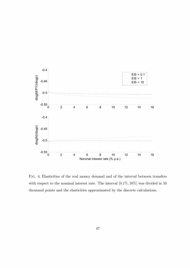
0 2 4 6 8 10 12 14 16-0.55
-0.5
-0.45
-0.4
dlog
(M/P
Y)/d
log(
r) EIS = 0.1EIS = 1EIS = 10
0 2 4 6 8 10 12 14 16-0.55
-0.5
-0.45
-0.4
dlog
(N)/d
log(
r)
Nominal interest rate (% p.a.)
Fig. 4. Elasticities of the real money demand and of the interval between transfers
with respect to the nominal interest rate. The interval [0.1%, 16%] was divided in 50
thousand points and the elasticities approximated by the discrete calculations.
47
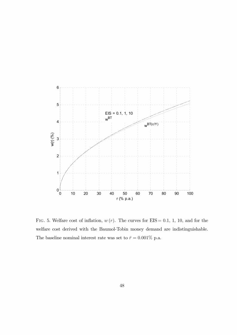
0 10 20 30 40 50 60 70 80 90 1000
1
2
3
4
5
6
EIS = 0.1, 1, 10wBT
wBT(c/Y)
w(r)
(%)
r (% p.a.)
Fig. 5. Welfare cost of inflation, w (r). The curves for EIS= 0.1, 1, 10, and for the
welfare cost derived with the Baumol-Tobin money demand are indistinguishable.
The baseline nominal interest rate was set to r = 0.001% p.a.
48
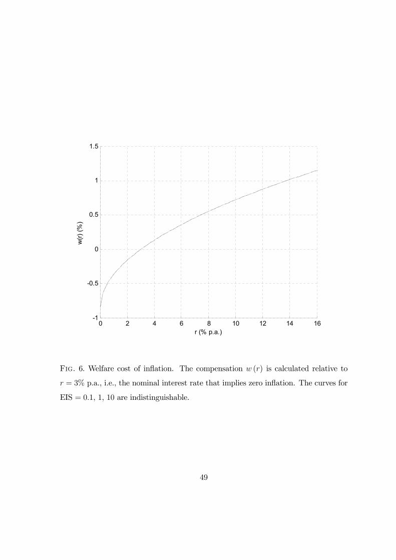
0 2 4 6 8 10 12 14 16-1
-0.5
0
0.5
1
1.5
w(r)
(%)
r (% p.a.)
Fig. 6. Welfare cost of inflation. The compensation w (r) is calculated relative to
r = 3% p.a., i.e., the nominal interest rate that implies zero inflation. The curves for
EIS = 0.1, 1, 10 are indistinguishable.
49
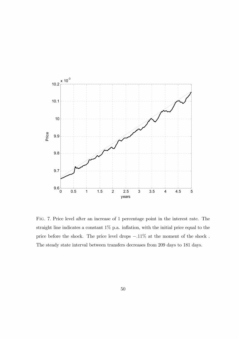
0 0.5 1 1.5 2 2.5 3 3.5 4 4.5 59.6
9.7
9.8
9.9
10
10.1
10.2x 10⁻³
years
Pric
e
Fig. 7. Price level after an increase of 1 percentage point in the interest rate. The
straight line indicates a constant 1% p.a. inflation, with the initial price equal to the
price before the shock. The price level drops −.11% at the moment of the shock .
The steady state interval between transfers decreases from 209 days to 181 days.
50
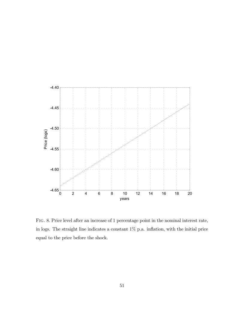
0 2 4 6 8 10 12 14 16 18 20-4.65
-4.60
-4.55
-4.50
-4.45
-4.40
years
Pric
e (lo
gs)
Fig. 8. Price level after an increase of 1 percentage point in the nominal interest rate,
in logs. The straight line indicates a constant 1% p.a. inflation, with the initial price
equal to the price before the shock.
51
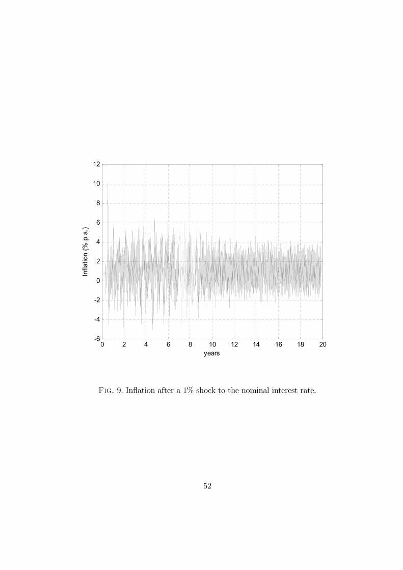
0 2 4 6 8 10 12 14 16 18 20-6
-4
-2
0
2
4
6
8
10
12
years
Infla
tion
(% p
.a.)
Fig. 9. Inflation after a 1% shock to the nominal interest rate.
52
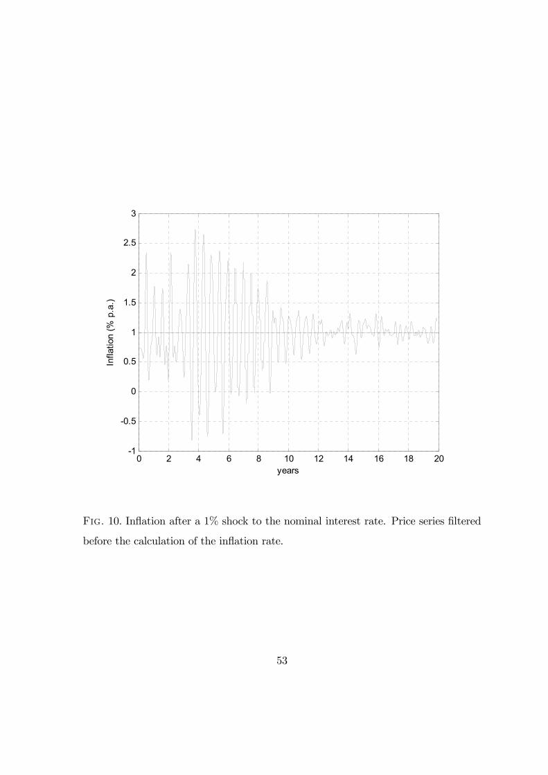
0 2 4 6 8 10 12 14 16 18 20-1
-0.5
0
0.5
1
1.5
2
2.5
3
years
Infla
tion
(% p
.a.)
Fig. 10. Inflation after a 1% shock to the nominal interest rate. Price series filtered
before the calculation of the inflation rate.
53
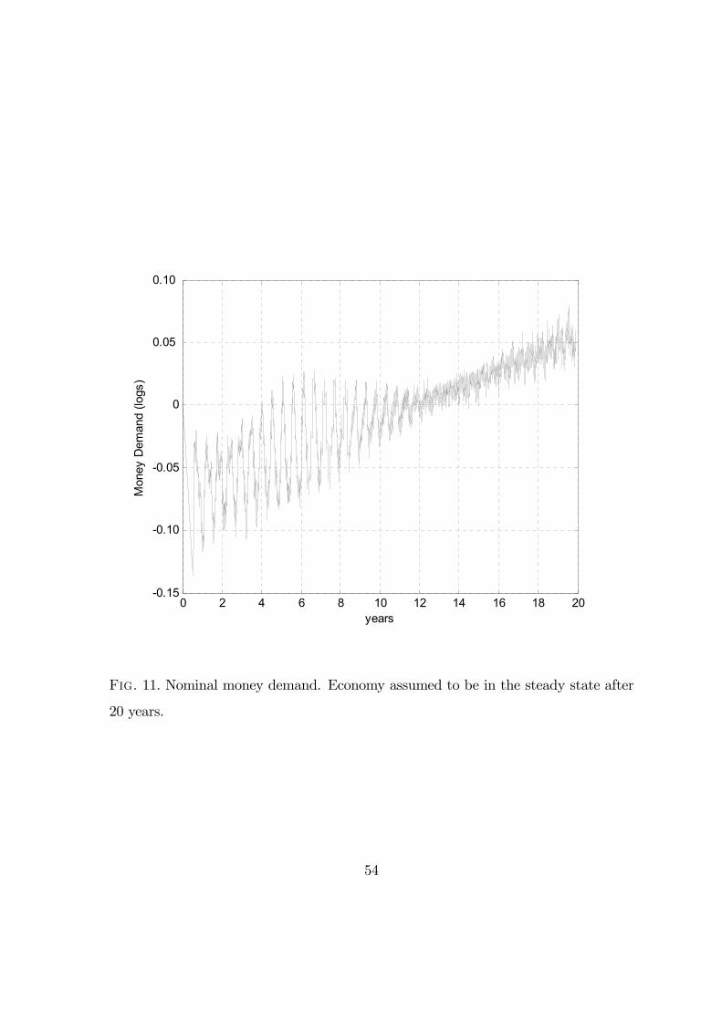
0 2 4 6 8 10 12 14 16 18 20-0.15
-0.10
-0.05
0
0.05
0.10
years
Mon
ey D
eman
d (lo
gs)
Fig. 11. Nominal money demand. Economy assumed to be in the steady state after
20 years.
54
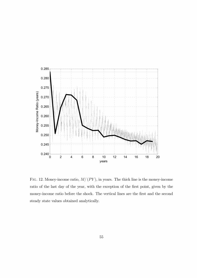
0 2 4 6 8 10 12 14 16 18 200.240
0.245
0.250
0.255
0.260
0.265
0.270
0.275
0.280
0.285
years
Mon
ey-In
com
e R
atio
(yea
rs)
Fig. 12. Money-income ratio,M/ (PY ), in years. The thick line is the money-income
ratio of the last day of the year, with the exception of the first point, given by the
money-income ratio before the shock. The vertical lines are the first and the second
steady state values obtained analytically.
55
REFERENCES
Alvarez, Fernando, Andrew Atkeson, and Chris Edmond (2002). “On the
sluggish response of prices to money in an inventory theoretic model of money
demand.” University of California, Los Angeles Working Paper.
Bailey, Martin J. (1956). “The Welfare Cost of Inflationary Finance.” Journal of
Political Economy, 64(2): 93-110.
Baumol, William J. (1952). “The Transactions Demand for Cash: an Inventory
Theoretic Approach.” Quarterly Journal of Economics, 66(4): 545-556.
Caplin, Andrew, and John Leahy (1997). “Aggregation and Optimization with
State-Dependent Pricing.” Econometrica, 65(3): 601-625.
Caplin, Andrew, and John Leahy (1991). “State Dependent Pricing and the
Dynamics of Money and Output.” Quarterly Journal of Economics, 106(3): 683-
708.
Christiano, Lawrence J., Martin Eichenbaum, and Charles Evans (1999).
“Monetary Policy Shocks: What We Have Learned and to What End?” Handbook
of Macroeconomics, Michael Woodford and John Taylor (eds.). Amsterdam: North
Holland.
Friedman, Milton (1969). “The Optimum Quantity of Money.” In Friedman, Mil-
ton, The Optimum Quantity of Money and Other Essays. Aldine: Chicago.
Fusselman, Jerry and Sanford Grossman (1989). “Monetary Dynamics with
Fixed Transaction Costs.” Princeton University Working Paper.
Grossman, Sanford J. (1987). “Monetary Dynamics with Proportional Transac-
tion Costs and Fixed Payment Periods.” In Barnett, William A. and Kenneth
56
J. Singleton (eds.), New Approaches to Monetary Economics. University Press:
Cambridge.
Grossman, Sanford J. and Laurence Weiss (1983). “A Transactions Based
Model of the Monetary Transmission Mechanism.” American Economic Review,
73(5): 871-880.
Harberger, Arnold C. (1998). “A Vision of the Growth Process.” American Eco-
nomic Review, 88(1): 1-32.
Jovanovic, Boyan (1982). “Inflation and Welfare in the Steady State.” Journal of
Political Economy, 90(3): 561-577.
Lucas, Robert E., Jr. (1990). “Liquidity and Interest Rates.” Journal of Economic
Theory, 50: 237-264.
Lucas, Robert E., Jr. (2000). “Inflation and Welfare.” Econometrica, 68(2): 247-
274.
Romer, David (1986). “A Simple General Equilibrium Version of the Baumol-
Tobin Model.” Quarterly Journal of Economics, 101(4): 663-686.
Romer, David (1987). “The Monetary Transmission Mechanism in a General Equi-
librium Version of the Baumol-Tobin Model.” Journal of Monetary Economics, 20:
105-122.
Rotemberg, Julio J. (1984). “A Monetary Equilibrium model with Transactions
Costs.” Journal of Political Economy, 92(1): 40-58.
Tobin, James (1956). “The Interest-Elasticity of the Transactions Demand for
Cash.” Review of Economics and Statistics, 38(3): 241-247.
57
Vissing-Jorgensen, Annette (2002). “Towards an Explanation of Household Port-
folio Choice Heterogeneity: Nonfinancial Income and Participation Cost Struc-
tures.” Working Paper.
58