monetary dynamics in a network economy
TRANSCRIPT

HAL Id: halshs-03165773https://halshs.archives-ouvertes.fr/halshs-03165773
Submitted on 15 Mar 2021
HAL is a multi-disciplinary open accessarchive for the deposit and dissemination of sci-entific research documents, whether they are pub-lished or not. The documents may come fromteaching and research institutions in France orabroad, or from public or private research centers.
L’archive ouverte pluridisciplinaire HAL, estdestinée au dépôt et à la diffusion de documentsscientifiques de niveau recherche, publiés ou non,émanant des établissements d’enseignement et derecherche français ou étrangers, des laboratoirespublics ou privés.
Monetary dynamics in a network economyAntoine Mandel, Vipin Veetil
To cite this version:Antoine Mandel, Vipin Veetil. Monetary dynamics in a network economy. Journal of Economic Dy-namics and Control, Elsevier, 2021, 125, pp.104084. �10.1016/j.jedc.2021.104084�. �halshs-03165773�

Monetary Dynamics in a Network Economy
Antoine Mandel∗ Vipin P. Veetil†
February 2, 2021
Abstract
We develop a tractable model of price dynamics in a general equilibrium economywith cash-in-advance constraints. The dynamics emerge from local interactions betweenfirms that are governed by the production network underlying the economy. Weanalytically characterise the influence of network structure on the propagation ofmonetary shocks. In the long run, the model converges to general equilibrium andthe quantity theory of money holds. In the short run, monetary shocks propagateupstream via nominal changes in demand and downstream via real changes in supply.Lags in the evolution of supply and demand at the micro level can give rise to arbitrarydynamics of the distribution of prices. Our model provides an explanation of the pricepuzzle: a temporary rise in the price level in response to monetary contractions. In oursetting, the puzzle emerges under two assumptions about downstream firms: they aredisproportionally affected by monetary contractions and they account for a sufficientlysmall share of the wage bill. Empirical evidence supports the two assumptions for theUS economy. Our model calibrated to the US economy using a data set of more thanfifty thousand firms generates the empirically observed magnitude of the price level riseafter monetary contractions.
JEL Codes C63, C67, D80, E31, E52Key Words Price Puzzle, Production Network, Money, Monetary Non-Neutrality, Out-of-Equilibrium Dynamics.
∗Paris School of Economics and Centrre d’Economie de la Sorbonne UMR CNRS 8174, Universite Paris 1Pantheon-Sorbonne. Maison des Sciences Economiques, 106-112 Boulevard de l’hopital 75647 Paris Cedex13, France. Mandel acknowledges the support of the EU H2020 programme through grant agreements ITNEXSIDE 721846, ITN EPOC 956107, and TIPPING+ 884565.†Department of Humanities and Social Sciences, Indian Institute of Technology Madras, Chennai, India
600036.
1

1 IntroductionA basic implication of the quantitative theory of money is that monetary contractionsinduce a decrease in the price level. However, numerous empirical studies report monetarycontractions generate a temporary increase in the price-level. This “price puzzle” is sizeable:a monetary contraction that generates a 0.1% decrease in the price-level in three years iscapable of generating a 0.1% increase in three months (Rusnak et al., 2013, Table 4). Thesizeable wrong directional movement in the price-level is significant because the price-levelmediates the relation between money and output in theoretical models of monetary neutrality(Lucas, 1972; Ball and Mankiw, 1994). Within sticky-price and sticky-information models ofmonetary neutrality, a wrong directional change in the price-level implies a counterfactualrelation between money and output (Mankiw and Reis, 2002). The Price Puzzle is thereforeempirically sizeable and theoretically significant.
In this paper, we show that the price puzzle can be explained by the propagation ofmonetary shocks through the production network of the economy. The propagation ofmonetary shocks generate differential and time-varying responses in the supply and demandfor consumer goods. The price puzzle emerges if monetary shocks have a strong short-term impact on the supply and a weak short-term impact on the demand of consumptiongoods. Two conditions prove sufficient to induce these dynamics: downstream firms must bedisproportionally affected by monetary contractions and they must account for a sufficientlysmall share of the wage bill, or more precisely sufficiently small to ensure that demand for finalgoods does not decline relative to supply following a monetary shock. Both conditions findempirical support. Also, our model calibrated to the US economy generates the empiricallyobserved magnitude of the wrong directional movement in the price-level following a monetarycontraction.
Our approach builds on Acemoglu et al.’s (2012) model of the network origins of aggregatefluctuations. We consider an economy with a representative consumer and a finite number offirms with Cobb-Douglas production functions. The production network of the economy isidentified with the weights of these Cobb-Douglas functions. We introduce two novel elementsin this framework. First, we consider prices are set locally by firms. Second,we assume firmsface cash-in-advance constraints.
These assumptions yield an analytically tractable model of price and monetary dynamics .Building on the existing literature emphasizing the heterogeneous impact of monetary
shocks on firms (Greenwald and Stiglitz, 1993; Holmstrom and Tirole, 1997; Clementi andHopenhayn, 2006), we model negative monetary shocks as (non-uniform) decrease of theworking capital of firms. A monetary contraction then affects both the demand and thesupply of consumer goods but through different mechanisms and with different time lags. Onthe demand side, firms hurt by the initial impact and subsequent propagation of a monetarycontraction decrease wages. The decrease in wages decreases the household’s income andtherefore the demand for consumer goods. The time necessary for a monetary contractionto generate the long run decrease in nominal demand for consumer goods depends on thetopology of the production network and the distribution of labor among firms. On the supplyside, firms hurt by a monetary contraction and its propagation temporarily decrease theiroutput as their inputs are bid away by competing users. This decrease in output propagates
2

downstream through the production network1.We then investigate how the propagation of monetary shocks affect price dynamics.
In the long run, the model converges to general equilibrium and the quantity theory ofmoney holds. In the short run, monetary disequilibrium propagates upstream via changes innominal demand and downstream via changes in real supply. In this setting, we analyticallycharacterise two conditions under which the price puzzle emerges. The first condition isfirms hurt by monetary contractions are sufficiently downstream. This condition guaranteesthat monetary contractions generate a decrease in the supply of consumer goods. Thesecond condition is firms hurt by monetary contractions bear a sufficiently small share of theeconomy’s wage bill. This condition guarantees that monetary contractions take sufficienttime to generate the long run decrease in the nominal demand for consumer goods.
Theory and data support the two aforementioned conditions. The first condition followsfrom the joint observation that downstream firms are disproportionately small and smallfirms are disproportionately hurt by monetary contractions (Gertler and Gilchrist, 1994;Gaiotti and Generale, 2002; Iyer et al., 2013; Carbo-Valverde et al., 2016).
Our second condition emphasizes that nominal demand decreases slowly because smallfirms which bear the brunt of the initial impact of monetary contractions account for alimited portion of the economy’s wage bill. Firms with annual receipts of less than one millionaccount for less than 8% of the wage bill in the US economy. Therefore the initial impact ofa monetary contraction generates a limited decrease in wages.
We further investigate the empirical validity of the model by calibrating it on the USproduction network using a novel data set with more than 100,000 buyer-seller relationsbetween more than 50,000 US firms including all major publicly listed firms. We use MonteCarlo methods to study the dynamics of the calibrated synthetic economy with computationalexperiments. In the experiments, the initial impact of monetary shock scales sublinearly withfirm size: small firms are disproportionately hurt by contractions. The model calibrated tothe US production network robustly reproduces the empirically observed magnitude of theincrease in price level after monetary contractions.
1.1 Related literatureThe existence of the Price Puzzle has been documented in a number of economies includingAustralia, France, Germany, India, Italy, Japan, United Kingdom, and the United States(Sims, 1992; Gaiotti and Secchi, 2006; Mishra and Mishra, 2012; Bishop and Tulip, 2017).Following the seminal work by Sims (1992) and Eichenbaum (1992), a large number ofcontributions have attempted to identify variables whose inclusion in VAR models wouldeliminate the puzzle.
Rusnak et al. (2013) present a meta analysis of the empirical literature on the subject.They find that about 50% of modern studies find a temporary rise in the price level followinga monetary contraction after controlling for a variety of variables. Similarly, Ramey (2016, p.
1A corollary of the argument is that a monetary contraction can increase the supply of consumer goods iffirms most hurt by the shock are sufficiently upstream. When firms far upstream are hurt by a monetarycontraction, downstream firms purchase more of the inputs used by both sets of firms by outbidding upstreamfirms. This allows downstream firms to expand the output of consumer goods.
3

36) finds most models of monetary policy shocks “are plagued by the Price Puzzle to greateror lesser degree”.
Against this background, three main types of explanations have been put forward in theliterature. the “common factors hypothesis”, the“reverse causation hypothesis”, and the“cost channel hypothesis”. The common factors hypothesis states that the price level increaseand monetary contraction are driven by common factors (Brown and Santoni, 1987). Theempirical performance of the common factors hypothesis is mixed. In a meta analysis ofempirical studies on the Price Puzzle, Rusnak et al. (2013) find that eight of eleven estimatesusing factor augmented VAR exhibit the Price Puzzle.
The reverse causation hypothesis states that the present monetary contraction is caused byfuture increase in the price level (Brissimis and Magginas, 2006; Barakchian and Crowe, 2013;Cloyne and Hurtgen, 2016). More specifically, present monetary contraction is a consequenceof a policy decision based on an expectation of a future increase in the price level. Thapar(2008) however finds the Price Puzzle to be present even after conditioning for the informationset of central banks. And Hanson (2004) finds no correlation between a variable’s abilityto forecast inflation and its ability to resolve the Price Puzzle. Ramey (2016) re-estimatesseveral models to control for all information available to the Federal Reserve. Her estimatesshow that the wrong directional movement in the price level does not dampen due to theexpansion of the information set, in fact it increases the price puzzle.
The cost channel hypothesis argues that an increase in the interest rate increases the costof production and therefore the price level (Barth III and Ramey, 2001)
However, since a negative monetary shocks entails a decrease in the quantity of money,the rise in prices of some goods must be more than compensated for by the fall in pricesof other goods. Our model presents an explanation for why those goods whose prices risehappen to be disproportionately represented in basket of consumer goods.
Our approach also emphasizes the role of the production network in monetary transmissionmechanisms. In this respect, our contribution is related to recent work on ‘micro to macrovia production networks’ (see e.g. Acemoglu et al., 2012; Di Giovanni et al., 2014; Carvalhoand Tahbaz-Salehi, 2018; Baqaee and Farhi, 2019; Moran and Bouchaud, 2019).
However, few of these contributions have investigated the role of production networks inmonetary transmission mechanisms. Notable “historical” exceptions are Cantillon (1755),Mises (1953), and Friedman (1961). Among contemporary contributions, Nakamura andSteinsson (2010) and Paston et al. (2018) show intermediate inputs amplify the impact ofmonetary shocks. Anthonisen (2010) formalises monetary dynamics on production networksusing an overlapping generations model. In a previous contribution, Mandel et al. (2019), westudy price dynamics on production networks using an agent-based computational model andshow, by means of simulations that there can be wrong-directional price movements followinga monetary shock. However the analysis in Mandel et al. (2019) (i) focuses only on the microlevel: it shows that certain prices move in the wrong direction but gives no evidence thatthis effect can scale up to the macro level, i.e. that the price level per se can move in thewrong direction, (ii) does not provide analytical results (it relies entirely on simulations), (iii)considers a “toy” simulation model rather than one calibrated on empirical data and (iv)more broadly does not discuss the empirical conditions under which the prize puzzle canmaterialize. Ò Ozdagli and Weber (2017) present the only notable empirical measure of therole of production network in transmitting monetary shocks. They attribute 50-85% of the
4

real effect of monetary shocks to propagation through the production network. Preliminaryempirical evidence therefore suggests the production network is a significant transmissionmechanism.
The rest of the paper is organized as follows. Section 2 presents the model. Section 3analytically characterizes the propagation of monetary shocks in the model and providessufficient conditions for the price level to increase after a monetary contraction. Section 4presents empirical evidence on the sensitivity of small firms to monetary shocks as well astheir contribution to the price level and to the wage bill in the US. Section 5 presents theresults of simulations performed with the model calibrated to granular data on more than100,000 buyer-seller relations between more than 50,000 US firms. Section 6 concludes thepaper. All proofs are in the Appendix.
2 Model
2.1 The general equilibrium frameworkWe consider a general equilibrium economy as in Acemoglu et al. (2012) with a finite numberof firms and a representative household. The firms and the differentiated goods they produceare indexed by M = {1, · · · ,n}. The household has index 0 and N = {0, · · · ,n} denotes theset of agents. The representative household inelastically supplies λ0 units of labor and has aCobb-Douglas utility function of the form:
u(x0,1, · · · ,x0,n) :=∏j∈M
xaj,00,j (1)
where for all j ∈ M, aj,0 ∈ R+ is the share of good j in the household’s consumptionexpenditures, thus ∑j∈M aj,0 = 1.
Each firm i ∈M has a Cobb-Douglas production function of the form
fi(xi,0, · · · ,xi,n) := λi∏j∈N
xaj,ii,j (2)
where λi ∈ R++ is a productivity parameter. For all j ∈M, aj,i ∈ R+ is the share of good jin firm i’s intermediary consumption expenditures, thus ∑j∈N aj,i = 1 and there are constantreturn to scale. We assume each firm uses a non-zero quantity of labor in its productionprocess, i.e. for all i ∈M, a0,i > 0. The production structure is a network with adjacencymatrix A= (ai,j)i,j∈N where ai,j > 0 if and only if agent i is a supplier of agent j and |ai,j |measures the share of good i in the production costs of j. The network economy is denotedby E(A,λ) and satisfies the following assumption.
Assumption 1. The adjacency matrix of the production network A is irreducible and aperi-odic.
The adjacency matrix A is irreducible if there exists a path between every two nodes inthe network, i.e. for every i, j ∈N, there exists t∈N such that Ati,j > 0. An irreducible matrixis aperiodic if there is no period in the length of cycles around any node, i.e. the greatest
5

common divisor of {k ∈ N | ∃i ∈NAki,i > 0} is 1. In our setting, mild sufficient conditions forirreducibility and aperiodicity can be expressed in terms of the relationship between firmsand the representative household. Given that each firm uses some labor in its productionprocess, the matrix is irreducible if each good enters the supply chain of at least one goodconsumed by the household (the production of a good not satisfying this condition would bezero at equilibrium). The matrix is aperiodic if at least one firm uses another good as aninput in its production process, i.e. if it is not the case that all firms produce using laboronly. To sum up, Assumption 1 holds in all but degenerate cases. The standard notion ofgeneral equilibrium can then be defined as follows for the network economy E(A,λ).
Definition 1. A collection (pi,xi, qi)i∈N ∈ RN+ × (RN+ )N ×RN+ of prices, intermediary con-sumption vectors, and outputs is a general equilibrium of E(A,λ) if and only if:
∀i ∈M, qi = λi∏j∈N
xaj,ii,j and q0 = λ0 feasibility (3)
∀i, j ∈N, xi,j := aj,ipiqipj
profit and utility maximization (4)
∀i ∈N,∑j∈N
xj,i = qi market clearing (5)
This definition is standard but for the fact that the condition for profit and utilitymaximization have been expressed directly through first order conditions. It also accountsfor the fact that profit at equilibrium is zero given there are constant returns to scale. UnderAssumption 1, there exists a unique general equilibrium in the economy.
Proposition 1. Up to price normalization, the economy E(A,λ) has a unique equilibrium(pi,xi, qi)i∈N ∈ RN+ × (RN+ )N ×RN+ , which moreover satisfies:
∀i ∈M, pi = 1λi
∏j∈N
(pjaj,i
)aj,i . (6)
Using the normalization p0 = 1, this can also be written as:
log(p) = (I−A′|M )−1γ (7)
where A′ denotes the transpose of A, A′|M its restriction to M and for all i ∈M, γi :=− log(λi)−
∑j∈Maj,i log(aj,i).
2.2 DynamicsBuilding on Gualdi and Mandel (2016), we introduce a simple discrete-time model of out-of-equilibrium dynamics in the network economy E(A,λ) in order to study the short-termeffects of monetary shocks on prices.
The defining characteristic of our approach is that we model local decision-making offirms without a central signal about prices or quantities. This implies agents must use a
6

decentralized mechanism to make decisions about prices they set, combinations of inputsthey demand, and quantities of output they produce.
Agents must hold money balances in order to engage in decentralized trades. We assumeeach agent i ∈ N initially holds a certain money balance m0
i ∈ R+ and denote by mti the
money balance of agent i in period t ∈ N. The money balances of the household correspondto its consumption budget. The money balances of a firm can be thought of as its workingcapital or as a credit line extended by funders. Each firm i ∈M initially holds a certain stockof output q0
i ∈ R+. More generally, we denote by qti ∈ R+ the stock of output of firm i atthe beginning of period t. The household supplies a constant quantity of labor qt0 = λ0 everyperiod. We study the dynamics of prices, quantities, and money balances which emerge fromsuch a setting.
With Cobb-Douglas production technologies the optimal allocation of the working capitalof a firm among intermediary inputs is independent of the prices of inputs. More specifically,given working capital mt
i firm i’s nominal demand to agent j ∈N is equal to aj,imti. Simi-
larly, the representative household’s optimal nominal demand to agent j is aj,0mt0 because
preferences are Cobb Douglas. Thus total nominal demand faced by agent j is ∑i∈N aj,imti.
For sake of parsimony and to remain as close as possible to the conventional equilibriumframework, as a first approximation we assume prices are fully flexible and thus each agentj ∈N sets its price in period t to:
ptj =∑i∈N aj,im
ti
qtj(8)
This has two implications. First, firms sell their complete stock of output every period andthus do not carry inventories. Second, the intermediary consumption of good j by firm i inperiod t, xti,j ∈ R+ is given by:
xti,j = aj,imti
ptj(9)
Hence, the production and the stock of output available next period is:
qt+1i = fi(xti) (10)
Finally, each firm i must determine the share of revenues to carry over as working capitalto the next period. In this paper, we consider a stylized setting in which all revenues arecarried over. Namely, we assume:
mt+1i =
∑j∈N
ai,jmtj (11)
Remark 1. Equation 11 implicitly conveys assumptions about the target profit rate of thefirm on the one hand and its demand expectations on the other hand.
• First, the choice of the share of revenues carried over as working capital for the nextperiod implicitly corresponds to the choice of the profit rate at a stationary state. Inour setting as all revenues are reinvested, the profit rate at a stationary state ought to
7

be zero. This ensures that the stationary state is consistent with general equilibrium(see Proposition 2 below). From a behavioural perspective, it amounts to consider thatcompetitive pressure, or threat to entry, is such that firms consider zero profit rate asthe benchmark.The model can be extended to a setting where firms pay a dividend, or an interest, to itsfunders by assuming that a firm with revenue m ∈R+ only uses a share µ ∈ [0,1] of therevenue as working capital for next period. Then, at a stationary state, the firm makesa profit of m−µm and the profit rate is (1−µ). This profit can be distributed to thefunders of the firm as dividends in case of equity funding, or interests in case of debtfunding. Our zero profit assumption corresponds to the case where µ= 1. Consideringan arbitrary µ ∈ [0,1] would not qualitatively change the linear structure of the modelnor our results about price dynamics. The notion of equilibrium would however slightlydeviate from the conventional one (see Gualdi and Mandel, 2016) and the model wouldhave an additional free parameter. We thus focus on the case µ= 1 below.
• Second, the fact that the working capital for next period is determined as a functionof the revenues of the current period only, amounts to assuming that the firms havemyopic expectations and assuming that nominal demand is stationary. This assumptionis consistent with the fact that all preferences and technologies in the economy are Cobb-Douglas and thus that nominal demand is a priori inelastic to price changes. However,this assumption neglects potential changes in the revenues, and thus in nominal demands,of customers. Furthermore, myopic expectations discard the possibility for the firm tosave cash for precautionary motives in the face of the variability of its own revenues(note however that such precautionary motives would be unnecessary at a stationarystate).
Equations (8) to (11) define a dynamical system on RN+ ×RN+ × (RN+ )N ×RN+ , which definethe trajectories of prices (pti)t∈Ni∈N , intermediary and final consumptions (xti)t∈Ni∈N , output (qti)t∈Ni∈Nand money balances (mt
i)t∈Ni∈N in the network economy E(A,λ). In particular, this dynamicalsystem provides an analytically tractable model of price dynamics with good properties ofconvergence towards equilibrium. Namely, the dynamics of prices can be characterized bythe following lemma:
Lemma 1. In the dynamical system defined by Equations (8) to (11), for all t ∈ N and forall i ∈M :
pt+1i = 1
λi
mt+2i
mti
∏i∈N
(ptjaj,i
)aj,i(12)
Furthermore, if p0 is an equilibrium price:
log(pt+1i ) = log(p0
i ) +t∑
τ=0
∑j∈N
Aτj,i logmt+2−τ
j
mt−τj
(13)
This lemma highlights the fact that price dynamics are eventually determined by monetarydynamics. In particular, the lemma underlines, through the term mt+2−τ
j /mt−τj , the role of a
8

two-period long budgetary cycle. Although production is instantaneous, inputs are purchasedusing revenues from the previous period (mt−τ
i ) and output is sold in the following period(yielding revenues mt−τ+2
i ). This 2-period cycle impacts the price dynamics as the firm setsits price by confronting the nominal demand in the period following the production withoutput produced using the revenues from the period preceding the production.
Remark 2. The existence of this 2-period cycle reflects lags in the accounting/budgetaryprocess rather than in the production process. This lag is somehow minimal. Indeed, inour setting, production is instantaneous. However, goods cannot be sold more than onceper period and thus there must be a one period lag between purchase of inputs and sale ofoutput. Moreover, if there is a cash-in-advance constraint, or more generally if the financingconditions of firms depend on observables (e.g. in case of bank credit), the purchase of inputsdepend on the revenues of the preceding period. Hence the two periods lag. If there is delayin production, the lag can be greater than two periods. More precisely, it is straightforwardto extend the model to a setting where the production process of firm i ∈M lasts for νi ∈ Nperiods, Equation 13 is then extended to
log(pt+1i ) = log(p0
i ) +t∑
τ=0
∑j∈N
Aτj,i log mt+2−τ
j
mt−τ−νjj
(14)
where price dynamics depend on monetary dynamics through the heterogenous distribution oflags (2 +νj)j∈M .
As monetary dynamics are linear according to Equation (11), we can use standard resultsfrom the theory of Markov chains to show the convergence of monetary holdings to aninvariant distribution and therefrom, using Lemma 1, the convergence of the system togeneral equilibrium. Namely, one has:
Proposition 2. Assume m0 > 0, q0 > 0 and p0 > 0. The only globally asymptotically stablestate of the dynamical system defined by equations (8) to (11) is the element (mi,pi,xi, qi)i∈N ∈RN+ ×RN+ × (RN+ )N ×RN+ such that:
m= Am (15)(p,x,q) is a general equilibrium of E(A,λ) (16)∑
j∈Mpjqj =
∑j∈M
mj . (17)
Moreover, there exists κ ∈ R+ such that for all m0 ∈ RN , one has:
‖mt−m‖ ≤ κρt (18)
where ρ is the second largest eigenvalue of A.
In the absence of exogenous shocks, the out-of-equilibrium dynamics introduced aboveconverges to the general equilibrium of the network economy E(A,λ). The level of prices iscompletely determined by the monetary mass in circulation. And in equilibrium the revenueof a firm is proportional to its eigenvector centrality (Equation 15). The speed of convergenceand thus the very notion of the long-run depends on the structure of the network throughthe second largest eigenvalue.
9
3 Monetary shocks and price dynamicsIn this section, we aim to analyze the impact of exogenous monetary shocks on price dynamics.As hinted at by Lemma 1, a potential channel for this impact is through changes in theworking capital of firms. Monetary policy cannot impact directly cash holdings of firms butif these holdings are associated to a form of external funding, e.g. a credit line offered by abank, the reduction of the latter mechanically induces a reduction of the former.
Accordingly, in the following, we represent a negative monetary shock as the reduction ofthe working capital available to firms2. More precisely, we assume (although we do not modelit explicitly) that the working capital of firms is financed by some form of external funding,e.g. a credit line. The economy is initially in an equilibrium state, which is in particular suchthat firms are not credit constrained. The monetary shock is assumed to reduce the creditline of firms, and thus their working capital, below the level required to sustain equilibrium.Hence, following the monetary shock, firms temporarily become credit constrained (as in e.g.Greenwald and Stiglitz, 1993; Clementi and Hopenhayn, 2006). As emphasized below, themonetary shock and the induced credit constraints are eventually resorbed by the adjustmentof the price level as the economy reverts back to equilibrium. We shall however mostly beconcerned with the rich set of transient dynamics that emerge from the heterogeneous initialimpact of monetary shock among firms.
More formally, we consider an economy E(λ,A) that is initially at an equilibrium(m0
i ,p0i ,x
0i , q
0i ) := (mi,pi,xi, qi). The economy faces a monetary shock at the end of period 0.
This shock is represented by a vector ε ∈ RN such that for all i ∈N the working capital ofagent i is shifted to mi+ εi. Shocks can have heterogenous impacts at the micro-economiclevel. The long-term behavior of the economy following the shock is completely determinedby Proposition 2. Namely:
Corollary 1. An economy at the equilibrium (mi,pi,xi, qi)∈RN+ ×RN+ × (RN+ )N ×RN+ subjectto a monetary shock ε ∈ RN converges, for the dynamical system defined by equations (8) to(11) to the new equilibrium (mi, pi,xi, qi) ∈ RN+ ×RN+ × (RN+ )N ×RN+ such that for all i ∈M :
mi = (1 + ι)mi and pi = (1 + ι)pi (19)
where ι=∑i∈N εi∑i∈Nmi
.
Hence in the long-run the the monetary shock and the induced credit constraints areresorbed by the adjustment of the price level and the economy reverts back to equilibrium.Moreover, the quantitative theory of money holds: prices adjust exactly to the quantity ofmoney in circulation. Our principle question is however the short run dynamics of pricesfollowing a monetary shock. What drives the short run dynamics of prices is the heterogeneityof shocks at the micro-level. It is straightforward to check using Equation 8 that if shocks arehomogeneous, i.e. if for all i, j ∈N εi/εj = mi/mj, prices adjust instantaneously to their new
2We neglect potential short-term credit constraints faced by households and thus assume their consumptionbudget is only indirectly impacted by the monetary shock, i.e. through changes in wages as the shockpropagates. Indeed, short-term credit to household is much less available than to firms, except in certaincountries such as the US.
10

equilibrium values. Non-trivial dynamics materialize only if the initial impact of monetaryshocks is heterogeneous., i.e. if εi/εj 6= mi/mj where either ε ∈ RN+ (positive monetary shock)or ε ∈ RN− (negative monetary shock) .
3.1 Introductory ExampleWe consider the circular economy introduced in Figure 1 to highlight the effects at play whenthe initial impact of monetary shocks is heterogeneous. Within the circular economy theconsumer assigns the same consumption budget to each firm and each firm uses a share 1/2 oflabor in its production process. Furthermore, each firm has a single supplier and a singlebuyer among firms. We assume the productivity parameter is such that λi = 2 for each firm.The household supplies n units of labor.
F1
F2
F3
F4
Fn
C0A=
0 1/2 . . . . . . . . . 1/21/n 0 . . . . . . . . . 1/2... 1/2
. . . 0... 0 . . . . . . ...... ... . . . . . . 0 ...
1/n 0 0 0 1/2 0
Figure 1: A circular economy with n firms, F1, · · ·Fn and a consumer C0. The consumerassigns the same consumption budget to each firm, each firm uses a share 1/2 of labor inits production process, has a single supplier and a single buyer among firms. Links aredirected from suppliers towards buyers. Thick lines correspond to weights of 1/2 thin linescorrespond to weights of 1/n. The matrix A is the adjacency matrix of the network where thefirst line (resp. column) corresponds to the revenues (resp. expenses) of the household andthe subsequent lines (resp. columns) to these of the firms.
In this framework, assuming total monetary mass is 3n, it is clear that at equilibrium allprices are equal to 1, each firm holds 2 units of working capital, produces 2 units of outputusing 1 unit of labor and 1 unit of input from its supplier. The household holds n units ofwealth and consumes 1 unit of every good. The equilibrium distribution of wealth, output,and prices are given by the following table.
agent 0 1 2 3 · · · nm n 2 2 2 2 2q n 2 2 2 2 2p 1 1 1 1 1 1
Suppose firm 1 receives a positive monetary shock of 2ε > 0 at the end of period 0. Theinduced change in demand for firm 1 leads to the following state in stage 1.
11

agent 0 1 2 3 · · · nm1 n 2 + 2ε 2 2 2 2q1 n 2 2 2 2 2p1 1 + ε/n 1 1 + ε/2 1 1 1m2 n+ ε 2 2 + ε 2 2 2
Following the shock, firm 1 increases its demand to firm 2 and the household. This raisesthe price of labor and of firm 2’s output. For firm 1 the rise in labor price is more thancompensated by its increase in working capital. Firm 1 thus increases its output. For theother firms the rise in the price of labor induces a decrease in output. The state at t= 2 isgiven by:
agent 0 1 2 3 · · · nm2 n+ ε 2 2 + ε 2 2 2
q2 n 2
√√√√ (1 + ε)2
(1 + ε/n)(1 + ε/2) 2√
11 + ε/n
2√
11 + ε/n
2√
11 + ε/n
2√
11 + ε/n
p2 1 + ε/2n2 + ε/n
2
√√√√ (1 + ε)2
(1 + ε/n)(1 + ε/2)
2 + ε/n
2√
11 + ε/n
2 + ε/2 + ε/n
2√
11 + ε/n
2 + ε/n
2√
11 + ε/n
2 + ε/n
2√
11 + ε/n
m3 n+ ε/2 2 + ε/n 2 + ε/n 2 + ε/2 + ε/n 2 + ε/n 2 + ε/n
The increase in nominal demand triggered by the initial shock at this stage is mainlyconcentrated on firm 3 and on the household. This implies firm 3 has to increase price givenoutput has not increased. Furthermore, the nominal demand faced by firm 1 is decoupledfrom the increase in its output. Therefore, firm 1 has to decrease its price. Thus a positivemonetary shock can induce both increase and decrease of prices in the short-run.
To simplify analysis, we assume n is large and discard the terms ε/n. This simplifies theexpression of the state in stage 2 to:
agent 0 1 2 3 · · · nm2 n+ ε 2 2 + ε 2 2 2
q2 n 2
√√√√ (1 + ε)2
(1 + ε/2) 2 2 2 2
p2 1√
1 + ε/2
(1 + ε)2 1 1 + ε/4 1 1
m3 n+ ε/2 2 2 2 + ε/2 2 2The shock propagates further through two effects on production. Firm 2 increases its
output because of the increase in nominal demand it faced. Firm n increases its outputbecause of the decrease in the price of the input it buys from firm 1. This leads to the
12

following state in stage 3 (neglecting terms of order ε/n):
agent 0 1 2 3 4 · · · nm3 n+ ε/2 2 2 2 + ε/2 2 2 2
q3 n 2 2
√√√√(1 + ε/2)2
(1 + ε/4) 2 2 2 2((1 + ε)2
1 + ε/2)1/4
p3 1 1√
1 + ε/4
(1 + ε/2)2 1 1 + ε/8 1 ( 1 + ε/2
(1 + ε)2 )1/4
m4 n+ ε/4 2 2 2 2 + ε/4 2 2
As for firm 1 in stage 2, the increase of output by firms 2 and n is not matched by correspondingincrease in demand. Both firms thus decrease prices.
In the following periods, the sequence of events “positive demand shock, increase of output,decrease in price, increase in output” propagates further. However, the size of the shockdecays progressively each period as a part of the shock is absorbed by the household whichredistributes demand uniformly among firms (through the term ε/n neglected in our analysis).Eventually, the shock is evenly distributed among firms generating a general rise in prices bya factor of 1 + 2ε/3n.
3.2 Network structure and transmission of shocksThe above example shows that the impact of a monetary shock can be ambiguous in theshort run. For example, a positive monetary shock can induce both increase and decrease inprices in the short run. The temporary volatility in prices generated by a monetary shockpropagates across the network through two channels. One, a direct channel whereby themonetary shock induces a change in demand for inputs. Two, an indirect channel wherebyfirms respond to changes in the prices of inputs.
More generally, the short-term dynamics of prices is related to the network structureas follows. From equation 11, we have mt = At(m0 + ε) = Atm0 +Atε = m0 +Atε. UsingEquation (13) we can completely characterize the dynamics of prices following a monetaryshock by the structure of the supply network. First, for t= 2, for all i ∈N :
log(p2i ) = log(p0
i ) + log(m3i
m1i
)+∑k∈N
Ak,i log(m2k
m0k
)(20)
= log(p0i ) + log
(m0i +A3
i,·ε
m0i +Ai,·ε
)+∑k∈N
Ak,i logm0
k +A2k,·ε
m0k
(21)
Equation (21) suffices to illustrate the main drivers of price dynamics. The primitive causeof the variation of prices is the non-uniform speed of propagation of monetary shocks acrossthe network. The shocks get propagated through walks of different lengths in the networkand thus reach a given node with different lags. This implies firms might experience changesin the nominal demand they face as highlighted by terms of the form mt+2
k /mtk. The changes
in nominal demand has a direct impact on prices corresponding to the term log(m3i/m1
i
)in
13

Equation (20). The direct channel induces a rate of change of prices that is proportionalto the rate of change of nominal demands. This direct impact propagates upstream in thenetwork: from buyers to sellers. The changes in nominal demand also has an indirect impactrepresented by the term ∑
k∈N Ak,i log(m2k/m0
k
), which corresponds to the feedback effect on
a firm from the changes in the prices of inputs induced by the direct demand effect. Thisindirect effect is mediated by the fact that changes in prices of the suppliers affects theproduction level of the firm and thus its price. The indirect effect propagates downstream inthe network: from sellers to buyers.
More generally, the relation between price dynamics, network structure, and shocks isgiven by:
log(pt+1i )− log(p0
i ) =t−1∑τ=0
∑k∈N
Aτk,i log m0
k +At+2−τk,· ε
m0k + ξ{τ<t}A
t−τk,· ε
(22)
where ξ denotes the indicator function.
A linear expansion of this expression highlights the relative role of upstream and down-stream propagation mechanisms. Namely, denoting by log(pt)∈RN the column vector formedby the log(pti) and by A′ the transpose of A, one has:
Proposition 3. For small enough monetary shocks ε, the dynamics of prices can be approxi-mated by:
log(pt+1)− log(p0) =t∑
τ=0(A′)τ∆mA
t−τ (A2− I)ε+ (A′)t∆mε (23)
where ∆m is the diagonal matrix whose coefficients are the (m0k)k∈N .
In line with the preceding discussion, Equation (23) highlights the fact that the primitivedriver of the dynamics is the volatility in nominal demand induced by the initial shock. Thisis represented by the term (A2− I)ε corresponding to the differences between the directimpact of the shock ε and its impact after a two period lag A2ε. As emphasized in Remark 2,the two period lag embodies the fact that inputs are purchased using the revenues from theprevious period and yield new revenues in the following period. This lag in the propagationof shocks creates a mismatch between supply and demand which is resorbed by a deviation ofprices from their equilibrium values. The size of this initial deviation (A2− I)ε is determinedby the local structure of the network. More precisely, it depends on the incoming degreeof order two i.e. the weights of incoming paths of length two. The initial price deviationis likely to be small if the network is homogeneous and the distribution of two-degrees iscentred around average (equal to one). If a node has a large incoming degree of order two i.e.it is a large indirect supplier of the economy, it is likely to initially react in an unconventionalmanner to a monetary shock. For example, the firm may decrease its price following a positivemonetary shock (indeed A2
i,·ε− εi is likely to be positive if ε ∈ RN+ ). Conversely, a node withsmall incoming degree of order two is likely to initially exacerbate the effect of a monetaryshock. This role of second order interconnectivity is reminiscent of the results in Acemogluet al. (2012).
This initial volatility is then propagated in the network. The propagation is representedby the linear operator ∑t
τ=0(A′)τ∆mAt−τ . The operator corresponds to the combination of
14

upstream/forward and downstream/backward propagation channels identified above. Theterm At−τ corresponds to the upstream propagation of the variation of demand and of thecorrelated variation of price from a firm to its suppliers. The term (A′)τ corresponds to thepropagation of the feedback effect induced by the price variation of a firm on the price ofits buyers through changes in production costs. Hence the term (A′)τAt−τ (A2− I)ε can beinterpreted as the propagation of the shock (A2− I)ε for t− τ steps in the upstream/forwarddirection and then for τ steps in the downstream/backward direction. In other words, theshock propagates through demand effects for t− τ steps via At−τ and through price effectsfor τ steps via (A′)τ . More formally, (A′)τAt−τ is the matrix of weights of walks of lengthn whose t− τ first steps are in the direction of the edges of the network and whose τ laststeps are in the opposite direction. The factor ∆m corresponds to the scaling of the shockproportionally to the initial monetary holdings. The operator ∑t
τ=0(A′)τ∆mAt−τ corresponds
(up to the rescaling factor ∆m) to the total weights of walks of length t in the network whenallowing for both forward and backward propagation. To sum up, the log-variation of priceat the end of period t+ 1, log(pt+1)− log(p0), corresponds to the propagation of the initialshock (A2− I)ε through the network in both forward and backward directions. The term(A′)t∆mε is a corrective term accounting for the fact that there is no variation of prices inperiod 0 to be propagated backwards.
Remark 3. The propagation operator is very similar to the matrix of weights of walksof length t upon which the computation of feedback centrality measures is based (see e.g.Bonacich, 1987; Jackson, 2010). Explicitly, if one discards the rescaling factor ∆m, one has∑tτ=0(A′)τAt−τ = (A+A′)t, which corresponds to the matrix with the walks of length t for the
adjacency matrix A := A+A′ of the undirected network obtained by discarding the directionof links in A. Thus, up to the rescaling factor ∆m, the cumulative logarithmic variation ofprices at time T, VT :=∑T
t=0 log(pt+1)− log(p0), is proportional to the sum of the Bonacichcentrality, truncated at time T, of the undirected network A with weights (A2− I)ε and of theoriginal network A with weights ε (see Ballester et al., 2006).
It is worth noting that the transient variations in nominal demand at a node i followinga shock mt+2
i /mti = (m0
i+At+2k,· ε)/(m0
i+Atk,·ε) are to a certain extend arbitrary. The transient
changes in demand are determined by the ratio between the weights of walks of differentlength leading from the sources of the shocks to the node under consideration. This ratio isdetermined by the structure of the network and can assume a wide range of value as discussedbelow (see Proposition 4). A foremost consequence of this remark is that a given monetaryshock can induce heterogeneous transient price response in different parts of the productionnetwork. In particular, a positive monetary shock could induce negative price change inthe short-run. In what follows, we derive the behavior of the distribution of prices and theprice-level in the course of the out-of-equilibrium propagation of monetary shocks.
3.3 The dynamics of the distribution of pricesAt the micro-economic level, empirical evidence suggests monetary shocks generate wrongdirectional movement in some prices. For instance, Lastrapes (2006) and Balke and Wynne(2007) find that about 50% of commodity prices change in the wrong direction in response to
15

monetary shocks3. Our model provides an explanation of the wrong directional movement insome prices.
Suppose a local positive shock induces an increase in the working capital of a firm i andconsequently its demand for inputs from firm j. Firm j is likely to increase its price. Howeverin so far as other buyers of firm j are not yet affected by the shock, the increase in price maybe less than the increase in demand by firm i. This allows firm i to purchase more inputsand increase output. Given the local nature of the shock, the increase in output may not bematched by a corresponding rise in demand faced by firm i. And thus firm i may decreaseits price next period. The price decrease induced by the intertemporal gap between supplyand demand faced by firms propagates upstream through the supply chain, i.e. it affects thesuppliers of the firm with a delay. Firm i’s price decrease creates a second source of potentialprice anomalies: following the price decrease, the buyers of firm i can increase their output.The process can lead to further decrease in prices if the increase in output is not matchedby a corresponding increase in demand. This effect propagates downstream through thesupply chain: from a firm to its buyers. These price anomalies progressively disappear as theinitial monetary shock diffuses in the network. Over time the increase in nominal demandbecomes uniform and is matched by a corresponding general rise in prices. In the long-runthe quantity theory of money holds.
As emphasized in Propositions 1 and 3, the magnitude and the duration of the priceanomalies are determined by the structure of the network and the characteristics of the initialshock. At the micro-economic level, the variations induced by the shock can be arbitrary.Namely, one has:
Proposition 4. For every finite sequence of prices p = (p0,p1, · · · ,pT ) ∈ RT+1+ such that
p1 ≥ p0, there exists a network economy E(A,λ), a monetary shock ε ∈ RN , and a firm i suchthat the sequence of prices of firm i in the T first periods is p.
More generally, according to Proposition 3, the dynamics of the price distribution iscompletely determined by the structure of the network.
3.4 The Price PuzzleNumerous econometricians have reported a short run increase in the price level in responseto monetary contractions (see e.g. Hanson, 2004; Rusnak et al., 2013, and references therein).Our model generates a rise in the price level if monetary contractions disproportionatelyaffect the suppliers of consumer goods but are transmitted to consumer’s final demand witha lag. Under these two conditions, in the short run the supply of consumer goods decreasesmore than the final demand thereby generating an increase in the prices of consumer goods.In what follows, we characterize a general class of “supply-chain” economies which generatean increase in the price level following a contractionary monetary shock.
We define a supply-chain economy as a network economy E(A,λ) together with a set of Llayers: {L1, · · · ,LL}. The set of layers form a partition of the set of firms M . A firm in layer `
3Balke and Wynne (2007) use data on monthly changes in the components of commodities Producer PriceIndex (PPI). At the highest level of disaggregation (the eight digit level) the data contains 130 time series in1959 to 1228 time series in 2001. Lastrapes (2006) uses data of 69 commodity price indexes with completemonthly observations from 1959:1 to 2003:10.
16

has all its suppliers in layer `−1 and all its consumers in layers `+1 (among firms). In otherwords, the adjacency matrix (restricted to firms) of the economy is upper triangular by block.This structure is very similar to the one considered in early contributions investigating thepropagation of shocks in production networks (Bak et al., 1993; Scheinkman and Woodford,1994; Battiston et al., 2007). We assume the household consumes goods produced by firmsin layer LL . The household’s supply of labor is normalized to 1. Let k denote the share oflabor supplied to layer LL at equilibrium. Assuming without loss of generality that the totalwealth is such that the price of labor is normalized to 1, one has:
k =∑i∈LL
a0,im0i and (1−k) =
∑j∈L−L
a0,jm0j (24)
where L−L denote the layers others than L.In this setting, suppose all firms in the LL are affected by an homogeneous negative
monetary shock of magnitude ρ: the working capital of each firm i in layer LL decreases to(1−ρ)m0
i . One has:Proposition 5. Assume the share of labor supplied to layer LL at equilibrium is k and thatthere is an homogeneous negative monetary shock of magnitude ρ on the firms of layer LL,then the price of firms of layer LL in period 2 is given by:
p2i = (1−ρk)a0,i+1
(1−ρ)a0,ipi,0. (25)
Corollary 2. Under the conditions of Proposition 5, for k sufficiently small, following anegative monetary shock, all consumer prices (i.e. all prices in layer LL) increase in theshort run (i.e. in period 2).
Under Corollary 2 a negative monetary shock induces a short-term increase (at leastin period 2) of the price level. Two conditions are sufficient for a rise in the price level inresponse to monetary contractions to emerge in the network economy. First, the shock mustbe sufficiently downstream (in layer LL). This condition ensures a monetary contractiongenerates a decrease in the supply of consumer goods. Second, firms initially affected bythe monetary contraction must bear a sufficiently low proportion of the economy’s wagebill (k must be sufficiently small). This condition ensures that the monetary contractiontakes sufficiently long time to generate the full long run decrease in final demand. The twoconditions jointly guarantee that in the short run supply decreases more than final demand,thereby generating an increase in the price-level in response to monetary contractions. Thelower the share k of downstream firms in the wage bill, the larger the discrepancy between thevariations of final supply and demand for consumer goods. And thus the more pronouncedthe rise in the price level after a monetary contraction as highlighted by Equation 25.
4 Empirical evidenceOur explanation of the price puzzle relies on three empirical assertions: (i) the fact thatsmall firms are disproportionally affected by monetary shocks, (ii) the fact that there is
17

a disproportionately high presence of small firms downstream and (iii) the share of smallfirms in the wage bill is small. Subsection 4.1 summarises the substantial evidence in theliterature that small firms are disproportionally affected by monetary shocks. Subsection4.2 presents empirical evidence supporting the claim that small firms are disproportionatelypresent downstream. Subsection 4.3 analyzes the share of small firms in the wage bill.
4.1 Empirical evidence on the impact of monetary contraction onsmall firms
There is substantial empirical evidence published in the literature supporting the claim thatsmall firms are disproportionally affected by monetary shocks.
• First, there is a direct empirical evidence that small firm are more affected by monetarycontractions in the US (Gertler and Gilchrist, 1994; Thorbecke and Coppock, 1996;Basistha and Kurov, 2008), Germany (Ehrmann, 2005), Japan (Masuda, 2015), andthe UK (Bougheas et al., 2006). Overall, there is a reallocation of all kinds of creditfrom small to large firms after a monetary contraction (Oliner and Rudebusch, 1996).
• Second, there is indirect evidence stemming from the fact firm size appears to havea significant impact on the response to monetary policy at the sectoral and regionallevels. Peersman and Smets (2005) and Dedola and Lippi (2005) find that variationin the impact of monetary contraction across sectors is partly due to variation in firmsize across the sectors. Similarly, the variation in the impact of monetary shocks acrossregions in the US is partly accounted for by variation in firm size across regions (Carlinoand DeFina, 1998). Overall the impact of monetary policy is not neutral to firm size.
• Finally, there is evidence that small firms face binding financial and liquidity con-straints (Froot, 1993; Carpenter and Petersen, 2002) and that these constraints affecttheir production decisions (BaÃśos-Caballero et al., 2002; Carreira and Silva, 2010;Chakraborty and Mallick, 2012). Accordingly, small firms are disproportionately af-fected by monetary contractions both through the bank-lending channel (Kashyapet al., 1996; Morgan, 1998) and the balance-sheet channel (Gaiotti and Generale, 2002;Ashcraft and Campello, 2007).
4.2 Small firms and price indices4.2.1 Variation in firm sizes across sectors
In what follows, unless otherwise explicitly stated ‘small firms’ mean firms with annualsales of less an a million USD. Figure 2 presents the share of small firms across sectors inthe US economy. The figure uses data from the Small Business Administration on the sizedistribution of the population of firms in the US economy pertaining to the year 2007. Figure2 shows that there is sizeable heterogeneity in the share of small firms across different sectorsof the US economy at the three digit NAICS-level. Sizeable heterogeneity at the three digitNAICS level exists with alternate definitions of small firms such as those with annual sales ofless than ten million USD. Furthermore, the heterogeneity exists both at higher and lower
18

levels of granularity. At the lowest level of granularity, we consider 1095 sectors4. At thislevel of granularity, firms with annual sales of less than ten million USD account for lessthan 1% of the total sales in 105 sectors, however they account for more than 10% of thetotal sales in 656 sectors. At the highest level of granularity, we consider nine major sectorclassifications5. Firms with annual sales of less than a million USD account about 20% theoutput of Services, while their share in Manufacturing, Mining, and Utilities is less than 2%.
4Of the 1095 sectors, 644 are at the NAICS six digit level, 378 at the five digit level, 72 at the four digitlevel, and 1 at the three digit level. All sectors are considered at the most granular level for which firm sizedistribution data is available.
5The major sectors are created by aggregating two digit NAICS sectors as follows: Agriculture: 11,Services: 61-62, 71-72, 81, Construction: 23, Retail: 44-45, Wholesale: 42, Manufacturing: 31-33, Mining: 21,Utilities: 22, Others: 48-56, 61-62.
19

Figure 2: The contribution of small firms to total sectoral sales. The figure takes “small firms”to mean firms with annual sales of less than a million USD.
4.2.2 Small firms and the price-level
The sizeable difference in the share of small firms suggests that in so far as small firmsrespond differently to monetary shocks (see Section 4.1), the response of a price index tomonetary shocks will depend on the sectoral composition of the index. We now present datato show the disproportionately high contribution of small firms to the basket of goods thatmake up the price-level. We consider two definitions of the price-level: Personal ConsumptionExpenditure (PCE) deflator and Consumer Price Index (CPI) Urban (The SupplementaryAppendix presents details on the construction of the CPI). We combine data from the BEA
20

on consumer expenditure across sectors with the data from SBA on size distribution of firmsacross sectors to determine the relation between the role of small firms in sector and theweight of the sector in the price-level. We find that sectors in which small firms accountfor more than 10% of the annual sales make up 14.7% of the economy, 34.8% of the PCE,and 48.8% of the CPI. In other words, sectors with a significant share of small firms havea higher representation in the price-level than in the economy, with these sectors playing asizeably greater role in the CPI than the PCE6. A more direct measure is the share of smallfirms in PCE rather than the share of sectors with a significant share of small firms. Thismeasure too suggests that small firms play a disproportionately high role in determining theprice-level7. More specifically, small firms account for 8.6% (resp. 9.4%) of the sales of basketof goods used to compute the PCE (resp. CPI) while their share in the economy is 4.4%.
Figure 3 compares the share of small firms in a sector to the relative importance of thesector in CPI, which is measured by the ratio between the share of the sector in the economyand its share in the CPI. More specifically, the figure considers the 53 sectors plotted inFigure 2. The x-axis of Figure 3 marks the share of small firms in the total sales of a sector.The y-axis marks the ratio of the share of a sector in CPI to its share in the economy, i.e.the disproportionally in a sector’s share in the price index. Pearson’s correlation coefficientbetween the variables on the x and y axis of Figure 2 is 0.22. The share of small firms ina sector is therefore positively correlated with its importance in the CPI. The correlationcoefficient declines to 0.09 when we consider PCE instead of CPI. This is consistent with theprevious observation about the higher presence of small firm sectors in CPI than in PCE.
6Note the basic mechanism of our model along with this empirical observation is consistent with thefinding that CPI exhibits greater wrong directional change than the PCE.
7We match sectors using the NAICS-BEA codes mapping provided by the BEA. Not all the sectoralclassification of the Input-Output are at the same NAICS digit level as the SBA size distribution. Exactmatching of NAICS codes accounts for about 78% of PCE, whereas fuzzing matching accounts for more than99% of PCE. Fuzzy matching of NAICS follows the simple rule of matching unmatched NAICS codes fromthe Input-Output table with up to 1-3 digit higher level codes.
21

Figure 3: Contribution of small firms to CPI. Slope and intercept of OLS regression line are0.13 and -0.07 respectively.
4.3 Share of small firms in the wage billWe measure the share of small firms in the wage bill of the economy using Small BusinessAdministration’s data on sectoral contribution to wages for the year 2007. Figure 4 presentsthe relation between size of firms and their share in the economy’s wage bill. The x-axispresent annual receipts. The y-axis presents cumulative share in wages. Figure 4 showsthat small firms do not account for the majority of the wage bill in the US economy. Morespecifically, firms with annual revenues of less than a million USD account for 8.6% of theeconomy’s wage bill, and firms with annual revenues of less than ten million US account forless than a third of the economy’s wage bill. Note that the share of small firms in the wagebill determines the initial impact of monetary contraction on nominal demand. The lowerthe share of small firms in the wage bill, the lower the initial decline in nominal demand, andtherefore the lower the initial decline in real supply necessary for the realization of the PricePuzzle.
A direct comparison between the 8.6% percent share of small firms in the wage bill andtheir 9.4% share in the PCE might suggest this difference is far from sufficient to generatethe Price Puzzle. Let us however first remark that the difference is more substantial whenthe CPI is taken into consideration as the share of small firms in the CPI is 10.7%. Thisdifference of more than 20% scales up when an alternative definition of small firms is used.Furthermore, the direct impact of the monetary shock on nominal demand and real supplymediated by small firms is more than proportional to their share in the wage bill and theprice index respectively because of the θ parameter. Finally, and more importantly, a majoramplification of the shock on real supply occurs through network effects: if small firms are
22

sufficiently downstream, upstream sectors will bid resources away from downstream sectors,thereby generating a decline in final output.
Figure 4: The plot marks the share of firms with different sizes in the wage bill of the economy.The y-axis is the cumulative wage bill. The x-axis is the log of the annual receipts with 17different sizes.
5 Computational experiments on the U.S. productionnetwork
Section 3 illustrates the emergence of an increase in the price level in response to a monetarycontraction within a stylised setting. In this section, we investigate the empirical relevance ofour model by calibrating it to granular data on the US production network. Furthermore,we extend the model to study the consequences of a more general distribution of monetaryshocks. Rather than assuming the initial impact of monetary shock falls upon firms in specificparts of the network, we allow all firms to bear the initial impact of monetary shocks albeitto different degrees. The magnitude of the initial impact of a monetary shock is inverselycorrelated to the size of the firm.
5.1 US firm network dataWe use firm-level data from S&P Capital IQ and Orbis BvD datasets to calibrate our model.Our data set includes 105,940 buyer-seller relationships between 51,913 firms for whom wehave revenue information and NAICS codes8. While the coverage of our data set is sparse
8S&P Capital IQ has a rich database about supply relationships between US firms from 2005 to 2017.We restricted the universe of firms to private firms and publicly listed firms. We excluded banks, non-
23

compared to the universe of US firms, it is nevertheless the most comprehensive dataseton supply relationships between US firms currently available. Our data set contains bothprivate and publicly listed firms whereas datasets used in previous studies on productionnetworks are limited to only contain listed firms (Atalay et al., 2011; Wu and Birge, 2014)or aggregated input-output network (Acemoglu et al., 2012). The inclusion of a subset ofnon-listed firms is relevant given the role of small firms in our explanation of the price puzzle.Figure 5 shows our data set matches the stylized fact that the degree distribution of theproduction network follows a power-law (Atalay et al., 2011; Konno, 2009). And Figure6 shows the revenue distribution of the firms in our data set follows a power-law like therevenue distribution of the universe of firms in the US (Axtell, 2001).
Figure 5: Degree distribution counter CDF.
banking financial corporations, and government entities. These restrictions left us with data on the businessrelationships between 80,092 US firms. Of the 80,092 firms Capital IQ provided data on revenues and NAICSsector codes for 43,321 firms. We used Orbis BvD to gather data on revenues or NAICS codes for 8,592 ofthe 36,771 firms with missing data. Completing the Capital IQ data set with information from Orbis BvDyielded a total of 105,940 supply relations between 51,913 firms for whom we know revenues and NAICSsectoral codes.
24

Figure 6: Annual revenues.
5.2 Baseline computational experimentsWe calibrate the model to US firms production network by assigning the matrix of observedsupply relationships as the adjacency matrix of the network. This matrix is however un-weighted (as Capital IQ does not collect the corresponding information). We use a tailoredalgorithm to calibrate the weights in such a way that the empirical distribution of revenues forthe firms is an invariant distribution of Equation 159. We also calibrate the network economyso that the households spending on different firms in our data set matches the sectoraldistribution of household personal consumption expenditure (PCE) in the Input-Outputtable. We then set the initial value of prices, money holdings, and stocks of output to theirequilibrium values. The system is initialized in the steady state—in the sense of Proposition2—corresponding to empirical observations about revenues and supply relationships.
We then run a series of computational experiments to investigate the dynamic responseof prices following a monetary shock. In these experiments, each time step of the modelis interpreted as a quarter on the basis of empirical observations about the frequency ofprice changes. Blinder (1991) for instance finds firms change prices in response to changesin cost and demand with the delay of a quarter. The monetary shocks considered in ourexperiments are constructed as follows. A first parameter s ∈ [0,1] measures the aggregatesize of the shock. A second parameter θ ∈ R+ measures the heterogeneity of the shockwith respect to firms’ sizes. Let M =∑
i∈Nmi denote the total money in circulation in theeconomy. A monetary contraction of size s removes sM units of money from circulation. Amonetary contraction is implemented through a reduction in the working capital of each firmi proportional to mθ
i . We focus on the case where θ < 1 when small firms are disproportionally9Estimating the network weights so that given firm sizes are the invariant distribution is a large matrix
quadratic programming problem. We solved the problem using IBM’s CPlex software.
25

affected by monetary contractions. The case θ > 1 would correspond to large firms beingdisproportionally affected by the contraction. While the case θ = 1 corresponds to the casewhere firms are homogeneously affected by the shock and prices instantaneously adjust totheir new equilibrium value (see Corollary 1).
We run series of computational experiments with variation in the size s of the monetaryshock and the heterogeneity θ of the initial impact of the shock. We focus on the dynamics ofthe price level measured using weights of the Personal Consumption Expenditure (PCE) fromthe Input-Output Table10. The figures below summarise data from about 500 computationalexperiments on the calibrated US economy with more than a million firm interactions.
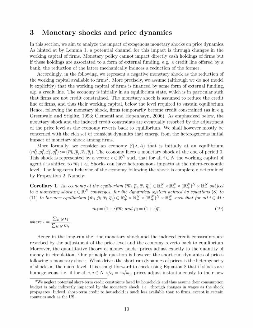
Figure 7 highlights a typical response of the system following a shock in that case. Thex-axis represents quarters, the y-axis represents the price-level. Since one time step of ourmodel represents one month, we average three month prices to compute the quarterly pricelevel. Figure 7 shows that the wrong directional change in the price level is of the same orderof magnitude as the long run right directional change. Furthermore, the wrong directionalchange in the price level generated by our model is on the same order of magnitude as thatwhich is reported by several empirical studies (see Rusnak et al., 2013).
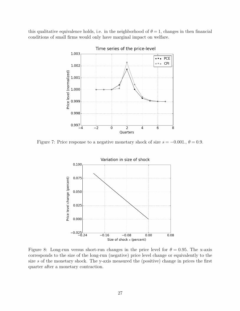
An increase in the price level after monetary contractions systematically occurs when smallfirms are disproportionally affected by monetary contractions for sufficiently low value of θ.The presence of the price puzzle is robust to changes in the magnitude s and the heterogeneityof the shock θ (for a sufficiently low value of θ). Figure 8 illustrates the sensitivity of themodel with respect to the strength of the monetary shock by showing the relation betweenthe size of the monetary contraction (that is measured indirectly by the long-run change inthe price level) and the size of the short-run change of the price level in the opposite direction.The y-axis in Figures 8 and 9 measure the percent change between the pre-shock price leveland the maximum price level in six quarters after a monetary contraction. Figure 8 showsthat the wrong directional change in the price level is of the same order of magnitude as thelong-term effect of the monetary contraction. Figure 9 illustrates the sensitivity of the pricelevel response with regards to the heterogeneity of the impacts. The response is non-linear11.The size of the price puzzle increases rapidly with the heterogeneity in initial impact ofmonetary shocks (|1−θ|). This highlights the importance of the correlation between networkstructure and firm size in the propagation of monetary shocks. Taking the magnitude ofthe price puzzle as an indirect indicator of the welfare losses during a monetary contraction,this sensitivity analysis implies that improving the financial conditions of small firms canhave positive welfare implications. Yet the non-linear response of the economy to a decreasein θ imply that a sizeable positive impact will materialise only if the financial conditions ofsmall firms become qualitatively similar to that of large firms. Outside of the range where
10The price level is computed in the following manner. The sectoral weights of the Personal ConsumptionExpenditure Index (PCE) are obtained from the Input-Output Table. The total weights of firms of a givensector in the price level is set equal to the share of that sector in the PCE. The total weight of a given sectoris equally divided among firms in that sector within our data set.
11Note that in Figure 9 a monetary contraction of size s=−0.001 does not cause a temporary increase inthe price level in the calibrated economy when θ > 0.97. This is simply because when θ is sufficiently highthe decrease is supply of consumer goods is overwhelmed by the short run decrease in the nominal demandfor consumer goods for the given size of monetary contraction. The exact value of θ beyond which monetarycontractions will not generate an increase in the price level will depend on the size of the contraction and thesize distribution of firms within the production network.
26
this qualitative equivalence holds, i.e. in the neighborhood of θ = 1, changes in then financialconditions of small firms would only have marginal impact on welfare.
Figure 7: Price response to a negative monetary shock of size s=−0.001., θ = 0.9.
Figure 8: Long-run versus short-run changes in the price level for θ = 0.95. The x-axiscorresponds to the size of the long-run (negative) price level change or equivalently to thesize s of the monetary shock. The y-axis measured the (positive) change in prices the firstquarter after a monetary contraction.
27

Figure 9: Short-run price level change as a function of the heterogeneity parameter θ for afixed size of monetary shock s=−0.001.
5.3 Impact of price rigidityWe investigate the sensitivity of our results to price rigidity by considering a variant of theprobabilistic price change model a la Calvo (1983). Namely, instead of considering that eachfirm i updates its price every period, we consider that it updates its price at time t with aprobability φti given by:
φti =( ρti
1 +ρti
)ψ(26)
where ψ ≥ 0 is a scaling parameter and ρti = |pt−1i −pti|pt−1i
with pt−1 the current price and pti theclearing price given by Equation 8. Note that the source of heterogeneity in the probability ofprice change is intrinsically related to the model dynamics we have empahized in explainingthe Price Puzzle. More specifically, after a monetary shock, firms that experience greaterchanges in their excess demands are more likely to change prices. And in so far as the networkpositions of firms determine the temporal sequence of the changes in money balances (andtherefore in excess demands), the network positions are intricately related to the probabilityof price change. More specifically, downstream firms are disproportionally hurt by the initialimpact of monetary contraction, they and their suppliers are more likely to change pricesin the early time steps after a monetary shock. As the shock propagates and dissipatesthrough the production network, all firms become less likely to change prices and thereforeless heterogeneous with regards to probability of price change.
We ran 100 computational experiments for each value of ψ ranging from 0.05 to 0.50with increments of 0.05. Figure 10 shows a time series of the price level from four of theseexperiments. The price-level increases in the transition from the pre-shock to the post-shockequilibrium. Figure 11 presents boxplots of the maximum price-level for different values of ψ.
28

Figure 11 therefore summarizes results from 1000 experiments (100 for each of the 10 valuesof ψ). The figure shows that a wrong directional change in the price-level is realized in allexperiments. Furthermore, the wrong directional response of the price-level declines withan increases in the scaling parameter ψ. This is because as ψ increase, the probability ofprice change decreases. The wrong directional change in the price-level is less pronouncedwhen fewer firms respond to monetary dynamics by changing prices. In other words, theprice puzzle is more likely to emerge if there is overshooting in the price adjustment process.
Figure 10: Time series of PCE after a monetary contraction with endogenous price-stickiness.Parameters: ψ = 0.1, s=−0.001.
29

Figure 11: Boxplot of maximum PCE after a monetary contraction with endogenous price-stickiness. Parameters: s=−0.001.
5.4 Structural change and the price puzzleAs we have access to a single dataset on the U.S. network, we can not empirically investigateimpacts of the network structure on price dynamics and the price puzzle in particular.However, Equation 18 in Proposition 2 highlights that the relaxation time of the economyto equilibrium depends on the second eigenvalue of the network. Thus, the duration, if notthe magnitude, of the price puzzle increases with the second eigenvalue of the network. Thesecond eigenvalue is a well-known measure of connectivity in graph theory (see e.g. Lovasz,2007). Notably, one can derive from an upper bound on the second eigenvalue, a lower boundon the edge and vertex connectivity of a graph12 (Abiad et al., 2017). Hence, productionnetworks with large second eigenvalues correspond to less diversified/integrated economies,whose sectoral components can easily be disconnected. This implies in particular, in linewith the findings in subsection 3.4, that the price puzzle ought to be more pronounced ineconomies with a clearcut separation between upstream and downstream sectors. In thisrespect, empirical evidence (Carvalho and Voigtlander, 2014) suggests that producers directtheir search for new inputs along vertical linkages, thus increasing the connectivity betweenupstream and downstream sectors and, incidentally, dampening the price puzzle.
Another structural limitation of our analysis is that we focus on Cobb-Douglas productionfunctions. Atalay (2017) finds that complementarities between inputs across sectors canamplify sector-specific productivity shocks. The basic dynamics of our model suggests thatcomplementarities between inputs across firms can amplify the wrong directional change in
12The edge (resp. vertex) connectivity is the minimal number of edges (resp. vertex) that must be removedfor the graph to become disconnected.
30
the price-level. Indeed, monetary contractions percolate through the production networkby inducing changes in relative prices or equivalently by inducing changes in the relativesupply/demand of different intermediate inputs. Thus, the lower the substitutability betweeninputs, the greater shall be the decline in output due to the decline in the supply of any giveninput (for any given increase in other inputs). The impact of monetary contractions on thereal supply of final goods shall therefore increase with an increase in input-complementarity.In so far as the wrong directional change in the price-level arises because the real supplyof final goods decreases more than the nominal demand for these goods, greater input-complementarity will exacerbate the price-puzzle by generating a greater decline in realsupply while leaving nominal demand for final goods unchanged.
Entry and exit processes might also interact with the propagation of monetary shocksto the extent that they modify the financial conditions of firms (or the average financialconditions within a sector). More specifically, in our setting, an increase in the liquidityavailable to small firms contributes to dampening the price puzzle. If, following a monetaryshock, small firms exit because of insolvency and are replaced by firms with a more sustainablefinancial structure but the same liquidity, there is no impact on the dynamics. If enteringfirms have better (worse) access to liquidity than exiting ones, entry might milden (resp.exacerbate) the price puzzle. This might in particular be the case if small exiting firms arereplaced or taken over by larger firms.
The role of the financial conditions of small firms on the transmission of monetary policyis well illustrated by the case of Germany. On the one hand, the strength of relationshiplending in Germany, notably via the hausbank model, leads to improved financial conditionsfor small firms (see e.g. Agarwal and Elston, 2001; Chatelain et al., 2003). On the other hand,the Price Puzzle is much less pronounced in Germany than in countries where commerciallending is predominant (see Sims, 1992; Rusnak et al., 2013).
6 ConclusionMore than 150 years ago, Thomas Tooke (1844, p. 85) observed that much of the data on therelation between money and the price-level shows conventional wisdom “is not only not true,but the reverse of the truth”. By conventional wisdom he meant the quantity theory of moneyrelation. Generations of economists since Tooke rediscovered the empirical phenomena undervarious guise including the ‘Price Puzzle’ and the ‘Gibson Paradox’ (Sargent, 1973). Despitethe empirical findings, most economist did not abandoned conventional wisdom (Laidler,1991). There are good reasons for this conservative attitude, not the least of which is theremarkable ability of the quantity theory to explain the long run co-movements in moneyand the price level (Lucas, 1996). Our paper reconciles the apparent contradiction between ‘apositive relation between money and the price-level in the long run’ with ‘a negative relationin the short run’. In constructing such a theory we did not resort to treating the price-level asthe independent variable and money as the dependent variable, nor did we let money and theprice-level be driven by common factors. Rather, we constructed a model in which monetaryshocks causally generate temporary wrong directional change in the price-level.
Unlike most models of monetary non-neutrality, within our model firms’ prices are fullyflexible. We introduced the production network as a mechanism for the transmission of
31

monetary shocks and let firm size distribution within the network influence magnitudes andtime-lags of changes in demand and supply of consumer goods. Under certain empiricallyplausible conditions, a monetary contraction causes supply of consumer goods to decreasemore than demand in the short-run, thereby generating an increase in the price-level. In thelong-run, real supply of consumer goods remains unchanged and nominal demand decreasesas the economy reaches a new equilibrium with a lower price-level.
We substantiated our theoretical results with computational experiments on the USeconomy. There is great scope to extend the empirical analysis. The network used inthis paper contains more firms and buyer-seller relations than hitherto available on the USeconomy. But our network data is two orders of magnitude short of the empirical reality.The US economy has more than six millions firm with employees related to each other on aproduction network. Our data set therefore contains fewer than one in every hundred firmsin the US economy (Axtell, 2001). Some of the structure of production must have beenlost in the truncation. The problem is particularly pronounced in the context of argumentsdeveloped in this paper because small firms which drive the dynamics of the price-level aretypically underrepresented in non-universal data sets of an economy’s production network13.We hope to have presented some motivations for the collecting detailed production networkdata to understand the dynamics of the price level: a variable of non-trivial significance forthe formulation of monetary policy.
13Within our setting the Input-Output table is no substitute for firm level network data. The Input-OutputTable does not contain the long supply chain linkages through which products pass from upstream producersto retail firms. More specifically, beginning from the final consumer any sector of the Input-Output Table canbe reached within two steps. This is certainly not true of the production network between firms. Within ourdata set of US firms network, some firms are up to seven steps away from the final consumer. The long chainsof flow of goods and money matter because they influence the time sequence and magnitudes of the responsesof supply and demand of consumer goods to monetary shocks, thereby shaping the behavior of the price-level.
32

ReferencesA. Abiad, B. Brimkov, X. Martinez-Rivera, O. Suil, and J. Zhang. Spectral bounds for the connectivity of
regular graphs with given order. arXiv preprint arXiv:1703.02748, 2017.
D. Acemoglu, V. M. Carvalho, A. Ozdaglar, and A. Tahbaz-Salehi. The network origins of aggregatefluctuations. Econometrica, 80(5):1977–2016, 2012.
R. Agarwal and J. A. Elston. Bank–firm relationships, financing and firm performance in germany. EconomicsLetters, 72(2):225–232, 2001.
N. Anthonisen. Monetary shocks in a spatial overlapping generations model. Journal of Economic Dynamicsand Control, 34(12):2461–2484, 2010.
A. B. Ashcraft and M. Campello. Firm balance sheets and monetary policy transmission. Journal of MonetaryEconomics, 54:1515–1528, 2007.
E. Atalay. How important are sectoral shocks? American Economic Journal: Macroeconomics, 9(4):254–80,2017.
E. Atalay, A. Hortacsu, J. Roberts, and C. Syverson. Network structure of production. Proceedings of theNational Academy of Sciences, 108(13):5199–5202, 2011.
R. L. Axtell. Zipf distribution of us firm sizes. Science, 293(5536):1818–1820, 2001.
P. Bak, K. Chen, J. Scheinkman, and M. Woodford. Aggregate fluctuations from independent sectoral shocks:self-organized criticality in a model of production and inventory dynamics. Ricerche Economiche, 47(1):3–30, 1993.
N. S. Balke and M. a. Wynne. The relative price effects of monetary shocks. Journal of Macroeconomics, 29(1):19–36, 2007.
L. Ball and N. G. Mankiw. A sticky-price manifesto. Carnegie-Rochester Conference Series on Public Policy,41:127–151, 1994.
C. Ballester, A. Calvo-Armengol, and Y. Zenou. Who’s who in networks. wanted: The key player. Econometrica,74(5):1403–1417, 2006.
D. R. Baqaee and E. Farhi. The macroeconomic impact of microeconomic shocks: beyond hulten’s theorem.Econometrica, 87(4):1155–1203, 2019.
S. M. Barakchian and C. Crowe. Monetary policy matters: Evidence from new shocks data. Journal ofMonetary Economics, 60:950–966, 2013.
M. J. Barth III and V. A. Ramey. The cost channel of monetary transmission. NBER MacroeconomicsAnnual, 16:199–240, 2001.
A. Basistha and A. Kurov. Macroeconomic cycles and the stock marketâĂŹs reaction to monetary policy.Journal of Banking & Finance, 32(12):2606–2616, 2008.
S. Battiston, D. D. Gatti, M. Gallegati, B. Greenwald, and J. E. Stiglitz. Credit chains and bankruptcypropagation in production networks. Journal of Economic Dynamics and Control, 31(6):2061–2084, 2007.
S. BaÃśos-Caballero, P. J. GarcÃŋa-Teruel, and P. MartÃŋnez-Solano. How does working capital managementaffect the profitability of spanish smes? Small Business Economics, 39(2):517–529, 2002.
J. Bishop and P. Tulip. Anticipatory monetary policy and the price puzzle. Reserve Bank of AustraliaDiscussion Paper 2017-02, 2017.
33

A. S. Blinder. Why are prices sticky? preliminary results from an interview study. Technical report, NBERWorking Paper No. 3646, 1991.
P. Bonacich. Power and centrality: A family of measures. American Journal of Sociology, 92(5):1170–1182,1987.
S. Bougheas, P. Mizen, and C. Yalcin. Access to external finance: Theory and evidence on the impact ofmonetary policy and firm-specific characteristics. Journal of Banking & Finance, 30(1):199–227, 2006.
S. N. Brissimis and N. S. Magginas. Forward-looking information in var models and the price puzzle. Journalof Monetary Economics, 53:1225–1234, 2006.
W. W. Brown and G. J. Santoni. Interest rates, commodity price changes, and gibson’s paradox. FederalReserve Bank of St.Louis Working Paper 1983-004, 1987.
G. A. Calvo. Staggered prices in a utility-maximizing framework. Journal of Monetary Economics, 12(3):383–398, 1983.
R. Cantillon. Essai Sur La Nature Du Commerce En General. 1755.
S. Carbo-Valverde, F. Rodrıguez-Fernandez, and G. F. Udell. Trade credit, the financial crisis, and smeaccess to finance. Journal of Money, Credit and Banking, 48(1):113–143, 2016.
G. Carlino and R. DeFina. The differential regional effects of monetary policy. Review of economics andstatistics, 80(4):572–587, 1998.
R. E. Carpenter and B. C. Petersen. Is the growth of small firms constrained by internal finance? Review ofEconomics and Statistics, 84(2):298–309, 2002.
C. Carreira and F. Silva. No deep pockets: Some stylized empirical results on firmsâĂŹ financial constraints.Journal of Economic Surveys, 24(4):731–753, 2010.
V. M. Carvalho and A. Tahbaz-Salehi. Production networks: A primer. Annual Review of Economics, 11,2018.
V. M. Carvalho and N. Voigtlander. Input diffusion and the evolution of production networks. Technicalreport, NBER Working Paper 20025, 2014.
A. Chakraborty and R. Mallick. Credit gap in small businesses: Some new evidence. International Journalof Business, 17(1):65–80, 2012.
J.-B. Chatelain, A. Generale, I. Hernando, U. von Kalckreuth, and P. Vermeulen. New findings on firminvestment and monetary transmission in the euro area. Oxford Review of Economic Policy, 19(1):73–83,2003.
G. L. Clementi and H. A. Hopenhayn. A theory of financing constraints and firm dynamics. The QuarterlyJournal of Economics, 121(1):229–265, 2006.
J. Cloyne and P. Hurtgen. The macroeconomic effects of monetary policy: A new measure for the unitedkingdom. American Economic Journal: Macroeconomics, 8(4):75–102, 2016.
L. Dedola and F. Lippi. The monetary transmission mechanism: evidence from the industries of five oecdcountries. European Economic Review, 49(6):1543–1569, 2005.
J. Di Giovanni, A. A. Levchenko, and I. Mejean. Firms, destinations, and aggregate fluctuations. Econometrica,82(4):1303–1340, 2014.
34

M. Ehrmann. Firm size and monetary policy transmissionâĂŤevidence from german business survey data. InIfo Survey Data in Business Cycle and Monetary Policy Analysis, pages 145–172. Springer, 2005.
M. Eichenbaum. Comments on interpreting the time series facts: The effects of monetary policy by sims.European Economic Review, 36(5):975–1000, 1992.
M. Friedman. The lag in effect of monetary policy. Journal of Political Economy, 69(5):447–466, 1961.
Froot. (Num), 1993.
E. Gaiotti and A. Generale. Does monetary policy have asymmetric effects? a look at the investment decisionsof italian firms. Giornale degli Economisti e Annali di Economia, 61(1):29–59, 2002.
E. Gaiotti and A. Secchi. Is there a cost channel of monetary policy transmission: An investigation into thepricing behavior of 2000 firms. Journal of Money, Credit, and Banking, 38(8):2012–2037, 2006.
M. Gertler and S. Gilchrist. Monetary policy, business cycles, and the behavior of small manufacturing firms.The Quarterly Journal of Economics, 109(2):309–340, 1994.
B. C. Greenwald and J. E. Stiglitz. Financial market imperfections and business cycles. The QuarterlyJournal of Economics, 108(1):77–114, 1993.
S. Gualdi and A. Mandel. On the emergence of scale-free production networks. Journal of Economic Dynamicsand Control, 73:61–77, 2016.
M. S. Hanson. The ‘price puzzle’ reconsidered. Journal of Monetary Economics, 51:1385–1413, 2004.
B. Holmstrom and J. Tirole. Financial intermediation, loanable funds, and the real sector. The QuarterlyJournal of Economics, 112(3):663–691, 1997.
R. Iyer, J.-L. Peydro, S. da Rocha-Lopes, and A. Schoar. Interbank liquidity crunch and the firm creditcrunch: Evidence from the 2007–2009 crisis. The Review of Financial Studies, 27(1):347–372, 2013.
M. O. Jackson. Social and Economic Networks. Princeton University Press, 2010.
A. K. Kashyap, J. C. Stein, and D. W. Wilcox. Monetary policy and credit conditions: Evidence from thecomposition of external finance: Reply. American Economic Review, 86(1):310–314, 1996.
T. Konno. Network structure of japanese firms. Economics: The Open-Access, Open-Assessment E-Journal,3:1–13, 2009.
D. Laidler. The quantity theory is always and everywhere controversial: Why? Economic Record, 67(4):289–306, 1991.
W. D. Lastrapes. Inflation and the distribution of relative prices: The role of productivity and money supplyshocks. Journal of Money, Credit and Banking, 38(8):2159–2198, 2006.
L. Lovasz. Eigenvalues of graphs. 2007.
R. E. Lucas. Expectations and the neutrality of money. Journal of Economic Theory, 4(2):103–124, 1972.
R. E. Lucas. Nobel lecture: Monetary neutrality. Journal of Political Economy, 104(4):661–682, 1996.
A. Mandel, D. Taghawi-Nejad, and V. P. Veetil. The price effects of monetary shocks in a network economy.Journal of Economic Behavior & Organisation, 164(1):300–316, 2019.
N. G. Mankiw and R. Reis. Sticky information versus sticky prices: a proposal to replace the new keynesianphillips curve. The Quarterly Journal of Economics, 117(4):1295–1328, 2002.
35

K. Masuda. Fixed investment, liquidity constraint, and monetary policy: Evidence from japanese manufac-turing firm panel data. Japan and the World Economy, 33:11–19, 2015.
H. Minc. Nonnegative matrices. Wiley, 1988.
L. Mises. The Theory of Money and Credit. Yale University Press, 1953.
A. Mishra and V. Mishra. Inflation targeting in india: A comparison with the multiple indicator approach.Journal of Asian Economics, 23(1):86–98, 2012.
J. Moran and J.-P. Bouchaud. Will a large economy be stable. Available at SSRN, 2019.
D. Morgan. The credit effects of monetary policy: Evidence using loan commitments. Journal of Money,Credit and Banking, 30(1):102–118, 1998.
E. Nakamura and J. Steinsson. Monetary non-neutrality in a multisector menu cost model. The QuarterlyJournal of Economics, 125(3):961–1013, 2010.
S. D. Oliner and G. D. Rudebusch. Is there a broad credit channel for monetary policy? EconomicReview-Federal Reserve Bank of San Francisco, pages 3–13, 1996.
A. Ozdagli and M. Weber. Monetary policy through production networks: Evidence from the stock market.NBER Working Paper No. 23424, 2017.
E. Paston, R. Schoenle, and M. Weber. The propagation of monetary policy shocks in a heterogeneousproduction economy. NBER Working Paper No. 25303, 2018.
G. Peersman and F. Smets. The industry effects of monetary policy in the euro area. The Economic Journal,115(503):319–342, 2005.
V. A. Ramey. Macroeconomic shocks and their propagation. NBER Working Paper 21978, 2016.
J. S. Rosenthal. Convergence rates for markov chains. Siam Review, 37(3):387–405, 1995.
M. Rusnak, T. Havranek, and R. Horvath. How to solve the price puzzle? a meta analysis. Journal of Money,Credit, and Banking, 45(1):975–1011, 2013.
T. J. Sargent. Interest rates and prices in the long run: a study of the gibson paradox. Journal of Money,Credit and Banking, 5(1):385–449, 1973.
J. A. Scheinkman and M. Woodford. Self-organized criticality and economic fluctuations. The AmericanEconomic Review, 84(2):417–421, 1994.
E. Seneta. Non-negative matrices and Markov chains. Springer Science & Business Media, 2006.
C. Sims. Interpreting the macroeconomic time series facts: The effects of monetary. European EconomicReview, 36(5):975–1000, 1992.
A. Thapar. Using private forecasts to estimate the effects of monetary policy. Journal of Monetary Economics,55(4):806–824, 2008.
W. Thorbecke and L. Coppock. Monetary policy, stock returns, and the role of credit in the transmission ofmonetary policy. Southern Economic Journal, 62(4):989–1001, 1996.
T. Tooke. An Inquiry into the Currency Principle: The Connection of the Currency with Prices and theExpediency of a Separation of Issue from Banking. Longman, Brown, Green, and Longmans, 1844.
J. Wu and J. R. Birge. Supply chain network structure and firm returns. SSRN Working Paper No. 2385217,2014.
36

A ProofsProof: (proof of Proposition 1 ). By substituting first-order conditions for profit maximiza-tion in the production technology of firms, one obtains for all i ∈M :
qi = λi∏
jÂă∈N
(aj,i
piqipj
)aj,i
Using the fact that ∑j∈Naj,i = 1, one can then factor out the term piqi to obtain equation 6 :
∀i ∈M, pi = 1λi
∏j∈N
( pjaj,i
)aj,i
Under the assumption that p0 = 1 and thus log(p0) = 0, this can be written in matricial formsas:
log( p) = At|M log(p) +γ (27)
where log(p) denotes the vector (log(p1), · · · , log(pn)) ∈Rn, At|M denotes the restriction to Mof At and for all i ∈M, γi :=− log(λi)−
∑j∈Maj,i log(aj,i).
Furthermore by combining the market clearing and the first-order conditions for profitand utility maximization, one obtains for all i ∈ n, the equation
pjqj =∑i∈N
aj,ipiqi
This can be written in matricial form as
pq = Apq (28)
where pq := (p0q0, · · · ,pnqn)Given that A is aperiodic and irreducible and p0q0 is fixed, it is a standard result from
the theory of non-negative matrices that there exist a unique solution to Equation 28(see e.g.Seneta, 2006) .
Moreover, given that for all i ∈M, a0,i > 0 and ∑j∈N aj,i = 1, it is clear that the sum oflines of At|M are all strictly less than one. It is then a standard result from the theory ofnon-negative matrices that the spectral radius of At|M is strictly less than one (see e.g. Minc,1988). This implies that (I−At|M ) is invertible and hence that Equation 27 has a uniquesolution given by:
log(p) = (I−At|M )−1γ
Equations 27 and 28 hence determine a unique vector of outputs q ∈ RN and normal-ized prices p ∈ RN . It is then straightforward to check that (p,q) induces a unique generalequilibrium in the sense of definition 1.
Proof: (proof of Lemma 1). Let us first show Equation 12 holds. Using Equations (8) to
37

(11) sequentially yields:
pt+1i = mt+2
i
qt+1i
= mt+2i
fi(xti)
= mt+2i
fi
(a0,imt
i
pt0, · · · , an,im
ti
ptn
)
= mt+2i
λi∏j∈N
(aj,im
ti
ptj
)aj,i
Then using the fact that ∑j∈N aj,i = 1, one gets:
pt+1i = 1
λi
mt+2i
mti
∏j∈N
(ptjaj,i
)aj,i(29)
As for 13, let us show by recursion it holds if p0is an equilibrium price and thus satisfiesEquation 6:
• For t= 1, using the preceding condition one has
p1i = m2
i
m0i
1λi
∏j∈N
(p0j
aj,i
)aj,i
Using equation 6 then yields:
p1i = m2
i
m0i
p0i
or equivalently:
log(p1i ) = log(p0
i ) + log(m2i
m0i
)
• Let us then assume the property holds up to rank t.One has according to Equation 29:
log(pt+1i ) =− log(λi) + log
(mt+2i
mti
)+∑j∈N
(aj,i log(ptj)−aj,i log(aj,i))
38

Hence, by recursion:
log(pt+1i ) =− log(λi)−
∑j∈N
aj,i log(aj,i) + log(mt+2i
mti
)
+∑j∈N
aj,i
log(p0j) +
t−1∑τ=0
∑k∈N
(Aτ )k,j log(mt+1−τk
mt−τ−1k
)which can equivalently be written as:
log(pt+1i ) =− log(λi)−
∑j∈N
aj,i log(aj,i) +∑j∈N
aj,i log(p0j) + log
(mt+2i
mti
)
+t−1∑τ=0
∑k∈N
(Aτ+1)k,i log(mt+1−τk
mt−τ−1k
)
log(pt+1i ) =− log(λi)−
∑j∈N
aj,i log(aj,i) +∑j∈N
aj,i log(p0j)+
+t∑
τ=0
∑k∈N
(Aτ )k,i log(mt+2−τk
mt−τk
)
which eventually yields using Equation 6:
log(pt+1i ) = log(p0
i ) +t∑
τ=0
∑k∈N
(Aτ )k,i log(mt+2−τk
mt−τk
)(30)
Proof: (Proposition 2). Given Assumption 1, the convergence of (mt)t∈N to m and thebound on convergence speed given by Equation (18) are straightforward consequences ofexisting results about Markov chains (see e.g. Seneta, 2006; Rosenthal, 1995). It is thenstraightforward using Equation 8 that pt0 =mt+1
0 and thus that pt0 converges towards m0.
To show the convergence of (pti)t∈N, we shall first show it is bounded above and bounded awayfrom 0.
• To show that pti is bounded away from 0, it suffices, using Equation 8, to show that (i)production of each firm is uniformly bounded above and that (ii) monetary holdingsfor each firm are bounded away from 0. The former follows from the fact that laborresources are bounded and for each i ∈M, a0,i > 0. The latter follows from the fact thatmt
0 is bounded away from 0 (using the fact that for each i ∈M, a0,i > 0) and from theirreducibility of A.
• To show that pti is bounded above, it suffices, using Equation 8, to show that (i) themonetary holdings of each firm are bounded above and (ii) the output of each firm isbounded below. The former follows directly from the fact that total monetary holdings isbounded above. The latter follows from the fact that given monetary holdings of eachfirm are bounded below and above, there is a minimal share µ > 0 of the output of its
39

supplier that the firm can purchase at each time step. Then, if ε > 0 denotes the minimallevel of output among firms in period t, one has for all i ∈M qt+1
i ≥ µa0,i(µε)1−a0,i andthus qt+1
i ≥ ε as soon as ε≤ µ1/a0,i . In other words, one has for all i ∈M, and all t ∈N,qti ≥min(µ1/a0,i ,minτ<t qτi ) and thus qti is bounded away from 0 as soon as for all i ∈M,q0i > 0.
The fact that for all i ∈M, (pti)t∈N is bounded above and bounded away from 0 implies thatfor all i ∈M, (log(pti)t∈N is bounded. Furthermore using Equation 12, one has for all i ∈Mand all t ∈ N
log(pit+ 1) =− log(λi)−∑j∈N
aj,i log(aj,i) + log(mt+2i
mti
) +a0,i log(pt0) +∑j∈M
aj,i log(ptj)
log(pt+1i ) =− log(λi)−
∑j∈N
aj,i log(aj,i) + log(mt+2i
mti
) +a0,i log(mt+10 ) +
∑j∈M
aj,i log(ptj) (31)
Let us then denote by Xt := (log(pti))i∈M , Yt = (log(mt+2i
mti
) + a0,i log(mt+10 ))i∈M and Zt =
(− log(λi)−∑j∈N aj,i log(aj,i))i∈M . One can then write Equation 31 in matricial form as:
Xt+1 = Z+Y t+A′|MXt (32)
where Y t converges to some Y ∈ RM because of the convergence of (mt)t∈N and ‖A′|M‖< 1because A is column stochastic and for all i ∈M,a0,i > 0.
Thus, one hasXt+1−Xt = Y t−Y t−1 +A′|M (Xt−Xt−1).
It is then straightforward to show that the sequence (Xt+1−Xt)t∈N can not have otheradherence value than 0. As it is bounded, it must then be that Xt+1−Xt tends towards 0.
Now, as (Xt)t∈N is bounded, it has at least an adherence value. Let us then considersuch a value X. Equation 32 implies that one must have X = (I −A′|M )−1(Z + Y ). Thisimplies that (Xt)t∈N has at most one adherence value/ As it is bounded, it must converge. Inother words, one has shown the convergence of (log(pit))t∈N for all i ∈M. One can deduce,by continuity, the convergence of (pt)t∈N. Equation 12 then implies that the limit of (pt)t∈Nindeed is the equilibrium price p. The convergence of (xt)t∈N and (qt)t∈N to their equilibriumvalues as well as Equation 17 are then obtained by substitution in the Equations (9) and (10).
Proof: (Proposition 3). For all i ∈N, one can write equation 22 as:
log(pt+1i ) = log(p0
i ) +t∑
τ=0
∑k∈N
(Aτ )k,i log1 +
(At+2−τk,· − ξ{τ<t}At−τk,· )εm0k + ξ{τ<t}A
t−τk,· ε
40

A linear expansion in ε then yields:
log(pt+1i ) = log(p0
i ) +t∑
τ=0
∑k∈N
(Aτ )k,i
At+2−τk,· − ξ{τ<t}At−τk,·
m0k
ε+o(ε)
where lim‖ε‖→0 o(ε) = 0. This yields
log(pt+1i ) = log(p0
i ) +t∑
τ=0
∑k∈N
(A′)τi,k1m0k
(At+2−τk,· − ξ{τ<t}At−τk,·
)ε+o(ε)
This can be written in matricial terms as
log(pt+1) = log(p0) +t∑
τ=0(A′)τ∆m0(At+2−τ − ξ{τ<t}At−τ )ε+o(ε)
where ∆m is the diagonal matrix whose coefficients are the m0k. This eventually yields:
log(pt+1) = log(p0) +(
t∑τ=0
(A′)τ∆mAt−τ (A2− I)ε+ (A′)t∆mε
)+o(ε)
Proof: (Proposition 4). We consider an economy with 2S firms, where S > T +1, such thatfirm 1 uses only labor in its production process, for every i≥ 2 firm i uses only the outputof firm i−1 as input and the household only consumes the output of firm 2S. Formally, itcorresponds to the adjacency matrix A= (Ai,j)i,j∈N such that aj,i = δ(j,i−1 [2S+1]) where δ isthe Kronecker symbol and [2S+ 1] indicates that the sum is modulo 2S+ 1. Explicitly:
A=
0 1 0 · · · 00 . . . . . . . . . ...... . . . . . . . . . 00 · · · 0 . . . 11 0 · · · · · · 0
We shall further assume that the productivity parameter is such that λi = 1 for each firm
and that the household supplies 1 unit of labor. In this framework, assuming total monetarymass is Np0 it is clear that at the initial equilibrium all prices are equal to p0, each agentinitially holds m0
i = p0 units of wealth, produces 1 unit of output using 1 unit of input andthe household provides one unit of labor and consumes one unit of good 2S.
Let us then restrict attention to vectors of shocks ε that affect only the S last firms, i.esuch that for all i ≤ S,εi = 0. We shall show that this vector of shocks can be chosen suchthat the induced sequence of prices for firm S is p. Indeed, in this simple setting, the pricevariation of firm S are completely determined by the monetary shocks received downstream inthe supply chain whose variations induce a volatility of demand and thus of price for firmS. The simple structure of then economy allows to derive analytically the expression of thisvolatility and then to choose the sequence of shocks generating the desired price sequence.
Let us first remark that Lemma 1 implies that, in our framework, one has for all i≥ 1
41

and all t ∈ N :pt+1i = mt+2
i
mti
pti−1
and for all t≤ Tmti =m0
i +Ati,·ε= p0 + εi+t.
Thus, one has for all i≥ 1 and all t≤ T :
pt+1i = p0 + εi+t+2
p0 + ξ{t>0}εi+tpti−1
where ξX denotes the indicator function of the set X. Noting that εi = 0 for all i ≤ S, astraightforward recursion then shows that, one has for all 1≤ t≤ T :
ptS−1 = pt−1S
Therefore, one has for all t≤ T :
pt+1S = p0 + εi+t+2
p0 + ξ{t>0}εi+tpt−1S
It is then straightforward to choose (εS+2, · · · , · · ·εS+T+1) such that
(p0S , · · · ,pTS ) = p.
This ends the proof.
Proof: (proof of Proposition 5 and of the corollary). We consider that all firms in layer Lare affected by an homogeneous negative monetary shock of magnitude ρ, i.e. the workingcapital of each firm i in layer L is decreased to (1−ρ)m0
i . Then, the nominal demand of laborof firms in layer L is reduced to ∑i∈LL a0,i(1−ρ)m0
i = (1−ρ)k while the demand of labor offirms in other layers is maintained at =∑
j∈L−L a0,jm0j = (1−k). Thus the supply of labor to
each firm in layer L is reduced by a factor (1−ρ)/1−ρk < 1 in period 1.As firms in layer L are the only consumers of the firms of layer L−1, their supply of inputs
is not modified by the negative shock on their nominal demand. Overall, the production of firm
i in layer L in period 1, and thus its supply in period 2 is reduced by a factor(
1−ρ1−ρk
)a0,i
In parallel, the revenues of the household in period 1, and thus her demand in period 2, arereduced to 1−ρk
The price of a firm i in layer L in period 2 is therefore given by:
p2i = (1−ρk)ai,0(
1−ρ1−ρk
)a0,i
q0i
= (1−ρk)pi,0(1−ρ1−ρk
)a0,i = (1−ρk)a0,i+1
(1−ρ)a0,ipi,0
where q0i is the initial production level and p0
i the initial, equilibrium, price.
42

One then has p2i ≥ p0
i if and only if (1−ρk)a0,i+1
(1−ρ)a0,i≥ 1 or equivalently:
a0,i+ 1a0,i
<log(1−ρ)log(1−ρk) (33)
It is then clear that Equation 33 holds as long as k is sufficiently small.
43