Quasi-Equilibrium Dynamics of the Tropical Atmosphere

Kerry Emanuel Massachusetts Institute of Technology

1. Introduction Compared to the extratropical atmosphere, the dynamics of the tropical atmosphere are poorly understood. The cornerstone of dynamical meteorology – quasigeostrophic theory and its contemporary encapsulation in potential vorticity thinking – works well in middle and high latitudes, where the motion is quasi-balanced over a large range of scales and where diabatic and frictional effects are usually small and can often be neglected on short time scales. For this reason, the dynamics of fundamental processes such as Rossby wave propagation and baroclinic instability are well understood, and owing to the steep energy spectrum of quasi-geostrophic turbulence, the evolution of the extratropical atmosphere can be predicted many days in advance. By contrast, much of what occurs in the tropical atmosphere is neither quasi-balanced nor adiabatic, and the thus the tools that have served middle and high latitude meteorology so well are poorly suited to understanding the Tropics. Moreover, most of the belt between the Tropics of Cancer and Capricorn is covered by ocean, and so, before the advent of satellites, the atmosphere in this region was poorly observed. Even though there have been remarkable advances in satellite remote sensing, it is still difficult to produce reliable analyses of wind and water vapor. Advanced data assimilation techniques that work well outside the Tropics yield questionable results in tropical regions, not only because of the paucity of observations but because global atmospheric models are often inconsistent in rendering such basic tropical phenomena as the Madden-Julian Oscillation (Slingo and coauthors, 1996). Poor models and sparse observations, together with the greater influence of convective and mesoscale phenomena, also make weather forecasting problematic. Under the circumstances, it is hardly surprising that tropical meteorology has advanced less rapidly than the meteorology of middle and high latitudes. The advent of better models and faster computers has led to the circumstance that numerical simulation of the tropical atmosphere, for all of its problems, has in many ways outpaced advances in conceptual understanding. It may be that ever improved model physics and resolution will someday overcome present obstacles to improved analysis and prediction and thereby obviate any practical need for improved understanding. But history teaches us that simulation without understanding can be perilous, and is in any case intellectually empty. Yet there has been very substantial progress over the lasts few decades in understanding tropical phenomena. It is my purpose here to present an overview of the most important cornerstones of that progress, and to offer some speculations about future directions. I begin, in the next section, by positing radiative-moist convective equilibrium as the logical starting point for understanding the Tropics, in much the same way that zonal wind in thermal wind balance is an important starting point for understanding extratropical dynamics. Yet the radiative-convective equilibrium state is by no means trivial, and there are subtleties about it that continue to elude understanding. Because it is a statistical rather than an actual equilibrium, the classical

analysis of the stability of such a state to small fluctuations is circumscribed by the requirement that the space and time scales of the fluctuations be sufficient to average over the random fluctuations of the equilibrium state, much as continuum mechanics is restricted to fluid motions on super-molecular scales. In section 3, I review the linear theory of small perturbations to radiative-convective equilibrium, focusing on the great simplifications that result from assuming that convection maintains moist adiabatic lapse rates. The phenomenon of moist convective damping is examined, and an overview is presented of possible energy sources for the perturbations, including surface fluxes and cloud-radiation interactions. The successes and failures of the linear theory to explain observed tropical phenomena are discussed. The theory of finite amplitude perturbations to radiative-convective equilibrium – in which deep convection is entirely suppressed in certain regions – is reviewed in section 4 and compared to observations of such phenomena as the Hadley and Walker circulations, monsoons, and tropical cyclones. Section 5 presents a few examples illustrating the application of quasi-equilibrium, and Section 6 presents a summary. 2. Radiative-convective equilibrium: A useful starting point In the absence of large-scale circulations, the tropical atmosphere would assume a state of radiative-moist convective equilibrium, in which the divergence of the net vertical radiative flux (shortwave and longwave) would be compensated by the convergence of the vertical flux of enthalpy in convective clouds, except for in a thin boundary layer next to the surface, in which ordinary dry turbulence would carry the flux. There is, of course, no guarantee that such a radiative-convective state is stable to large-scale perturbations, and there is now considerable evidence that it is not. This in no way obviates its utility as an equilibrium state, though it may pose problems for its numerical simulation. The canonical problem of radiative-dry convective equilibrium was first developed by Prandtl (1942). In this problem, a semi-infinite but Boussinesq atmosphere subject to constant radiative cooling overlies a surface of fixed temperature. Assuming high Reynolds Number turbulence, there is only one external control parameter in the problem, the surface buoyancy flux, sF ; this is also proportional to the longwave radiative flux at infinity. On dimensional grounds alone, one may deduce that the

turbulence kinetic energy scales as ( )2

3sF z , where z is the altitude above the surface,

while the unstable stratification decreases as 4

3z− . This fully turbulent convecting fluid does not support any waves. Later work on the finite version of this problem (Deardorff, 1972) demonstrated that the turbulence kinetic energy throughout the layer scales as

( )2

3sF h , where h is the layer depth.

One easy variant of the classical Prandtl problem replaces the lower

boundary by a water surface, but assumes that any condensed water remains suspended in the air; i.e., there is no precipitation. Under these circumstances, most of the air is water-saturated. As in the classical dry problem, the turbulent enthalpy flux is known at each altitude, since it must balance the imposed radiative flux, but here the system specific enthalpy, k , is given by

,p vk c T L q= + (1) where pc is the heat capacity at constant pressure, T the temperature, vL the latent heat of vaporization, and q the mass concentration of water vapor. Since the entire system is water saturated, q is given by its saturation value, *q , which, by the Clausius-Clapeyron equation, is just a function of temperature and pressure. Thus the buoyancy flux has a direct relationship to the known enthalpy flux (as in the dry problem), and it can be shown that at each level, the buoyancy flux is reduced from its dry counterpart by the factor

2

2

*1

*1

v

d

v

p v

L qR T

L qc R T

+

+,

where dR and vR are the gas constants for dry air and water vapor, respectively. This is just the ratio of the moist adiabatic and dry adiabatic lapse rates and is always less than unity, showing that for an imposed radiative flux, the buoyancy flux will be less than in the dry case. In our atmosphere, this factor can be as low as 0.3. But in other respects, the saturated Prandtl problem is nearly isomorphic to the classical problem, and once again, the fluid is everywhere unstably stratified and does not support waves. The fun begins when one allows condensed water to precipitate. This deeply irreversible process depletes water from the ascending, cloudy currents, causing much of the descending air to be subsaturated and, owing to partial re-evaporation of the falling rain, driving strong downdrafts. As shown by Bjerknes (1938), the dry air between clouds is stably stratified and the asymmetry in stability to upward saturated displacements versus downward, unsaturated displacements causes a profound asymmetry in the fractional area occupied by up- and down-drafts. For Earth-like conditions, the updrafts occupy a very small fractional area, so that most of the fluid is unsaturated and stably stratified, thereby supporting buoyancy oscillations. Since air outside of clouds is generally subsaturated, the enthalpy flux (1) no longer specifies the buoyancy flux but instead acts as a constraint on the upward flux of water. As of this writing, there exists no generally accepted theory for the buoyancy flux in the precipitating Prandtl problem, though it can be shown to be necessarily less than that of the saturated Prandtl problem for the same imposed enthalpy flux. Although there is presently little understanding of precipitating radiative-convective equilibrium, there have been a number of numerical simulations approximating this state in doubly periodic domains and capped by a stable layer that represents the stratosphere. These simulations use nonhydrostatic models that explicitly, albeit crudely, simulate the convective cells themselves while at the same time having large enough domains to simulate many cells simultaneously. The surface temperature is generally fixed at a constant value, while internal radiative cooling is either calculated or imposed. Examples of three-dimensional simulations of radiative-convective equilibrium include those of Islam et al. (1993), Robe and Emanuel (1996) and Pauluis and Held (2002). Among the important results of these simulations are:

1) Convection maintains a nearly moist adiabatic lapse rate from cloud base to the tropopause;

2) As expected, active updrafts occupy only a very small fraction of the domain at any

one time; 3) In the absence of imposed shear, the convection is disorganized but more nearly

regular than random; i.e., cells are less likely to be adjacent than if they were truly randomly distributed. But in at least some models, convection appears to self-aggregate even in the absence of shear (Bretherton and Khairoutdinov, 2004);

4) Imposing a background wind with vertical shear organizes convection in squall lines

or arcs; these arcs may be parallel to the shear, perpendicular to it, or at an odd angle to it; depending on the shear profile;

5) Momentum transport by the convection is broadly downgradient but highly nonlocal; 6) Increasing the forcing (i.e. the imposed rate of radiative cooling) results in increased

spatial and temporal density of clouds but does not change the characteristic updraft velocities.

This latter point is interesting, but so far lacks a theoretical explanation. Although explicit simulations of radiative-convective equilibrium have shed light on a number of important aspects of such states, they are very expensive and it is still not quite possible to perform such simulations in domains large enough to contain internal waves with wavelengths much greater than characteristic intercloud spacing. Thus it has not been possible, so far, to explicitly simulate in three dimensions the interaction between convection and circulations large enough in scale to consider the convection to be in statistical equilibrium with the larger scale. 3. Behavior of small perturbations to the equilibrium state

a. Conditions for statistical equilibrium in perturbations

We now inquire about the disposition of small perturbations to radiative-

convective equilibrium. But since the equilibrium is statistical, the nature of the problem

depends very much on the scale of the perturbations. Convection itself is a chaotic

process, and introducing perturbations on the scale of the convective clouds themselves

can be expected to change the details of the state, but not its statistical properties. For

example, an internal gravity wave introduced at a scale smaller than that of the

characteristic intercloud spacing will rapidly lose its coherence amid the chaos of small

scale gravity waves excited by individual convective events. As with the continuum

hypothesis in statistical mechanics, great simplifications can be made by considering

perturbations large enough in space and long enough in time to average over many

convective cells, so that the convection may be approximated as remaining in statistical

equilibrium with the larger scales. This point was first emphasized by Arakawa and

Schubert (1974). On the other hand, there is little appreciation of just how large

perturbations need to be to meet the requirement of statistical equilibrium. Judging from

the results of explicit simulations of radiative-convective equilibrium, where the intercloud

spacing is on the order of several tens of kilometers, perturbations need to have scales

of at least 100 km to "see" the convective state as a continuum. But when vertical shear

is present, the spacing of squall lines in radiative-convective equilibrium simulations is

on the order of several hundred kilometers, so in that case statistical equilibrium might

only apply at scales more than 1,000 km or so. This suggests that statistical equilibrium

will never be as good an approximation, even for planetary scale phenomena, as the

continuum hypothesis is for geophysical fluid flows. Certain macroscale atmospheric

phenomena may prove as susceptible to the chaos of convection as a dust particle in

Brownian motion is to random molecular fluctuations.

In spite of these pessimistic considerations, much progress in tropical

meteorology is arguably attributable to the success of statistical equilibrium theory.

Virtually all global climate and weather prediction models, and most regional models,

rely on the parameterization of convection, which is as dependent on the notion of

statistical equilibrium as the Navier-Stokes equations are on the continuum hypothesis.

And, although it is not generally recognized outside the tropical meteorology community,

statistical equilibrium theory made several concrete predictions about tropical

phenomena that were later verified by observations.

b. Formulation of statistical physics

The cornerstone of the contemporary statistical equilibrium theory of convection

was first stated by Arakawa and Schubert (1974), who postulated that moist convection

consumes potential energy at the rate it is provided by larger scale processes. (They

called this the "quasi-equilibrium" hypothesis.) Thus potential energy, as quantified for

example by the "convective available potential energy" or "CAPE", does not accumulate

in the atmosphere but is released by convection as fast as it is produced. This

hypothesis, when coupled with a detailed model of how clouds redistribute enthalpy and

water, provides a closed representation of convective heating and moistening in terms of

large-scale variables. The Arakawa-Schubert formulation places no restrictions on the

actual amount of CAPE available at any given time; nor does it require CAPE to be

strictly invariant, any more than quasi-geostrophy requires flows to be steady. Quasi-

equilibrium is highly analogous to first order closure in turbulence theory, which

postulates that dissipation of turbulence kinetic energy locally balances generation.

Energy (or buoyancy) -based closures have now largely replaced earlier, Kuo-type

representations of moist convection based on the statistical equilibrium of water rather

than energy.

For simplicity and conceptual transparency, we here work with a somewhat more

restrictive formulation of quasi-equilibrium which proves more amenable to analytical

treatment. This formulation rests on two assumptions:

1) Moist convection always acts to maintain a moist adiabatic (virtual) temperature

profile, and

2) Convection always acts to maintain the neutral buoyancy of air lifted from the

subcloud layer to levels above cloud base.

These general notions have been implemented in two ways. The first, and simplest, is to

rigidly enforce both 1) and 2) above; this has sometimes been called "strict equilibrium".

The second involves relaxing the actual atmospheric state toward the satisfaction of 1)

and 2) over some finite time scale; this is often referred to as "relaxed equilibrium". The

use of 1) has been advocated by Betts (1986), Emanuel (1987), Yano and Emanuel

(1991), Neelin and Yu (1994), and Emanuel et al. (1994), among others. Assumption 2)

was introduced by Raymond (1995) and applied by many others.

In the spirit of simplicity, we will examine the behavior of small amplitude

perturbations to radiative-convective equilibrium states using the above approximations.

By "small", we mean literally infinitesimal; at any rate, we do not here consider

perturbations large enough to shut down deep convection anywhere. One working

definition of "nonlinear" as applied to this problem is "sufficient to shut off deep

convection somewhere in the perturbation". As we shall see in section 4, the transition

from "linear" to "nonlinear" thus defined may be fairly sharp.

c. Empirical restrictions on the validity of statistical equilibrium

Before continuing, it is worthwhile to examine the theoretical and empirical bases

for quasi-equilibrium in general and the restricted definition given by 1) and 2) above in

particular. First, the neutral state for moist convection is one in which the temperature

lies along a moist adiabat and for which boundary layer air lifted vertically is precisely

neutral. Convection is a comparatively fast process, and it is not unreasonable to

assume that it is efficient in driving the observed state toward criticality, much as the dry

convective boundary layer is always observed to have a dry adiabatic lapse rate, except

very near the surface. But there are several potential problems with moist criticality.

First, it may be objected that real convective clouds are observed to entrain

environmental air, greatly reducing their average buoyancy; thus a state that is neutral to

strictly adiabatic ascent would be quite stable to an entraining plume. Second, there is

the nontrivial question of how to define a moist adiabat. The buoyancy of air lifted

reversibly, for example, will be noticeably less than air lifted pseudo-adiabatically, in

which the condensed water loading is absent. There is also the problem of how and if to

include the ice phase, since supercooling of liquid water is common in clouds and thus

phase equilibrium cannot be assumed.

Yet observations of real convective clouds show that they are poorly modeled as

classical, entraining plumes. In the latter, studied extensively in the laboratory (Morton,

1956), entrained fluid is assumed to be instantly homogenized across the plume,

yielding a single buoyancy or a one parameter buoyancy distribution. Real clouds are,

however, highly inhomogeneous, containing a broad spectrum of mixtures, including

some air that has ascended nearly adiabatically (Paluch, 1979). This observation nicely

explains the paradox identified by Warner (1970), that real clouds are both highly dilute

and ascend nearly to levels predicted by adiabatic ascent of subcloud air.

Tropical (and many extratropical) temperature soundings are, to a first

approximation, moist adiabatic. Figure 1 is a buoyancy diagram, plotting the difference

between the density temperature1 of a reversibly lifted parcel and that of its environment,

as a function of the level from which the parcel is lifted (abscissa) and the level to which

it is lifted (ordinate). The ice phase has been ignored here, and the buoyancy has been

averaged over an entire year (about 1400 soundings) from Kapingamoranga in the far

western tropical Pacific. Note that the environment is precisely neutral (to within

measurement error) to a parcel lifted reversibly from around 950 hPa. This seems to be

a ubiquitous feature of the Tropics (Xu and Emanuel, 1989), though one may question

the relevance of the reversible adiabatic process. Figure 2 shows a time series from the

same tropical station comparing the density temperature of a sample lifted reversibly

from 950 hPa to the pressure-weighted vertical mean density temperature of its

environment. A running average of 10 days has been applied to the lifted parcel density

temperature, while the vertically averaged density temperature of the environment has

been smoothed over 2 days. There is a reasonably good correspondence between

fluctuations of the two quantities, suggesting that on these time scales, convective

criticality is a fairly good approximation. When the quantities are smoothed over shorter

times, the correspondence is less good, though it is not clear whether this is more

because criticality is a weaker approximation or because of measurement error. (The

lifted parcel temperature is particularly sensitive to the water content of the sample,

which suffers from relatively large measurement error. For example, a relative humidity

error of 5% in the boundary layer yields a 2.5 K error in the temperature of a parcel lifted

to 200 hPa. Thus to reduce the noise to a level comparable to the observed signal of

order .5 K in the free tropospheric temperature, one needs to average over around 25

soundings, or 8 days.) Figure 3 compares the mean density temperatures of the lower

and upper troposphere, smoothed over 2 days. Once again, there is good

correspondence, particularly of the low frequency components, suggesting that

assumption 1) above is reasonable.

There is still considerable uncertainty about the space and time scales over

which quasi-equilibrium may hold. Brown and Bretherton (1995) compared MST

temperature observations to measurements of boundary layer entropy fluctuations and

1 The density temperature is defined so that multiplying by the gas constant for dry air and dividing by pressure gives the actual inverse density. Its relationship to temperature and water substance is given by

( )1t

qT T qρ ε= + − , where q is the mass concentration of water vapor, qt is the mass concentration of all

water in the sample, and ε is the ratio of the molecular weight of water to that of dry air.

concluded that strict equilibrium can only be applied on time scales longer than about 40

days. Islam et al. (1993) analyzed space-time variability of precipitation in an explicit

three-dimensional simulation of radiative-convective equilibrium and concluded that

averaging over several hours and around 100 km is necessary to appreciably reduce the

variance produced by the chaotic behavior of individual convective cells. To illustrate the

process by which perturbations to moist equilibrium decay, we first ran a single-column

model into a state of radiative-convective equilibrium and then introduced a small

perturbation to the equilibrium state. The single column model uses a parameterization

of moist convection developed by Emanuel and Živković-Rothman (1999) as well as a

sophisticated radiative transfer formulation, and applied a fixed ocean temperature and

time-invariant clouds. Figure 4 shows the decay with time of a temperature perturbation

of peak magnitude 3 K introduced into the equilibrium state at 450 hPa. The temperature

perturbation spreads vertically while decaying over a time scale of roughly 12 hours, but

it also clearly has an oscillatory component with a period of around 5 days.

Taken together, these findings suggest that convective equilibrium fails on time

scales shorter than around 2 days and space scales less than around 100 km, but a

more precise determination of these limiting scales awaits further research.

d. Implications of the moist adiabatic lapse rate for the structure of tropical disturbances

Now consider the structure of hydrostatic perturbations to radiative-convective

equilibrium states in which moist adiabatic lapse rates are strictly enforced. We shall

slightly simplify the definition of "moist adiabatic" to the state in which the saturation

moist entropy, *s , is invariant with altitude. This quantity is defined as the specific

entropy air would have were it saturated with water vapor at the same temperature and

pressure. It is given approximately by2

0 0

** ln ln ,vp d

L qpTs c RT p T = − +

(2)

2 See Emanuel , K. A., 1994: Atmospheric Convection. Oxford Univ. Press, New York, 580 pp for an exact definition.

where 0T is a reference temperature, 0p is a reference pressure, and the other symbols are as defined previously. We shall show now that the requirement that *s remain constant with height places strong constraints on the structure of perturbations. Denoting perturbations from radiative-convective equilibrium by primes, the hydrostatic equation in pressure coordinates may be written

' 'pφ α∂

= −∂

, (3)

where φ is the geopotential and α is the specific volume. Ignoring virtual temperature effects, we regard α as a function of the two state variables p and *s . Fluctuations of α at constant p can then be written

*

' * ' * ',* p s

Ts ss pαα

∂ ∂ = = ∂ ∂ (4)

where in the second part of (4) we have made use of one of Maxwell's relations (Emanuel, 1994). The quantity in brackets on the far right side of (4) is just the moist adiabatic lapse rate. Substituting (4) into (3) and integrating in pressure gives ( )' '( , , ) ( , , ) * ',b x y t T x y t T sφ φ= + − (5) where T is the pressure-weighted vertical mean temperature in the troposphere. We have chosen the integration constant so that 'bφ is the pressure-weighted vertically averaged geopotential perturbation in the troposphere. Thus we can interpret 'bφ as the barotropic component of the geopotential perturbation. This shows that in a moist adiabatic atmosphere, geopotential perturbations associated with hydrostatic motions consist of a barotropic part plus a "first baroclinic mode" contribution with a single node in the troposphere. This latter has a vertical structure dictated by the shape of a moist adiabat. The restrictive vertical structure of geopotential perturbations indicated by (5) also constrains the structure of horizontal velocity. In particular, the linearized inviscid momentum equations show that both horizontal velocity components must have a structure identical in form to (5). Integrating the hydrostatic version of the mass continuity equation,

u v

p x yω ∂ ∂ ∂= − + ∂ ∂ ∂

with height (pressure) gives

( ) ( )( )0

0 0* *' ,

pb bp

u v u vp p p p T Tdpx y x y

ω ∂ ∂ ∂ ∂

= − + − − − + ∂ ∂ ∂ ∂ ∫ (6)

where ω is the pressure velocity, 0p is the surface pressure and we have represented the baroclinic parts of the horizontal velocities u and v with asterisks. Thus the structure of the vertical velocity is the accumulated difference between the temperature along a moist adiabat and its vertical mean value. By the definition of T , the second term on the right of (6) vanishes when ω is evaluated at the tropopause, so

( )0b b

t tu vp px y

ω ∂ ∂

= − + ∂ ∂ , (7)

where the subscript t denotes evaluation at the tropopause. Thus if we apply a rigid lid at the tropopause, we then require that the divergence of the barotropic component of the velocity vanish. In the linear undamped system, there is then no coupling between the baroclinic and barotropic motions, and the latter are independent of the former. We shall see later that the barotropic component must be present if we allow wave radiation into the stratosphere, and/or the baroclinic and barotropic components are coupled through surface friction or nonlinearity. The observed tendency of the tropical atmosphere to maintain moist adiabatic lapse rates is consistent with the prominence of first baroclinic mode structure in tropical disturbances, as first noted by Reed and Recker (1971) and Madden and Julian ( ), among others, and collapses the linear inviscid primitive equations into shallow water equations. What is left to determine is the feedback of perturbation motions on the temperature. e. Feedback of air motion on temperature In the classical theory of dry wave motions in the tropical atmosphere, first formulated by Matsuno (1966), the wave motions influence temperature by adiabatic warming and cooling associated with vertical air motion. Here we regard as "canonical" the problem of the disposition of an infinitesimal internal wave launched into a state otherwise in radiative-convective equilibrium, with the restriction that we must consider waves whose space and time scales are large compared to characteristic scales associated with the convection, so that statistical equilibrium may be assumed. It is clear from the outset that such perturbations cannot even crudely be considered (dry) adiabatic. But for the sake of simplicity, in what follows we shall neglect all diabatic effects except for those associated with the phase changes of water. Convection only redistributes enthalpy and so cannot alter the mass-weighted vertical enthalpy given by (1). Thus the moist static energy, h , given by the sum of the specific enthalpy and the specific potential energy, can only be changed by large-scale advection. In the absence of horizontal advection and perturbations to the surface enthalpy flux and the radiative cooling, the evolution of the vertically integrated enthalpy is given by

,hkdp dpt p

ω∂ ∂= −

∂ ∂∫ ∫ (8)

where the integral is over the depth of the troposphere and ω is the wave-associated vertical motion. Using tropical sounding data, Neelin and Held (Neelin and I. M. Held, 1987) showed that the observed structure functions of ω and h p

∂∂ in the Tropics yield

negative integrated enthalpy tendency when air is ascending. From (1), we have

p vT qc dp kdp L dpt t t

∂ ∂ ∂= −

∂ ∂ ∂∫ ∫ ∫ . (9)

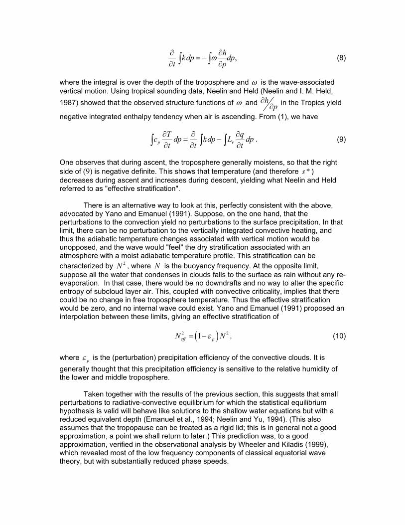
One observes that during ascent, the troposphere generally moistens, so that the right side of (9) is negative definite. This shows that temperature (and therefore *s ) decreases during ascent and increases during descent, yielding what Neelin and Held referred to as "effective stratification". There is an alternative way to look at this, perfectly consistent with the above, advocated by Yano and Emanuel (1991). Suppose, on the one hand, that the perturbations to the convection yield no perturbations to the surface precipitation. In that limit, there can be no perturbation to the vertically integrated convective heating, and thus the adiabatic temperature changes associated with vertical motion would be unopposed, and the wave would "feel" the dry stratification associated with an atmosphere with a moist adiabatic temperature profile. This stratification can be characterized by 2N , where N is the buoyancy frequency. At the opposite limit, suppose all the water that condenses in clouds falls to the surface as rain without any re-evaporation. In that case, there would be no downdrafts and no way to alter the specific entropy of subcloud layer air. This, coupled with convective criticality, implies that there could be no change in free troposphere temperature. Thus the effective stratification would be zero, and no internal wave could exist. Yano and Emanuel (1991) proposed an interpolation between these limits, giving an effective stratification of ( )2 21eff pN Nε= − , (10) where pε is the (perturbation) precipitation efficiency of the convective clouds. It is generally thought that this precipitation efficiency is sensitive to the relative humidity of the lower and middle troposphere. Taken together with the results of the previous section, this suggests that small perturbations to radiative-convective equilibrium for which the statistical equilibrium hypothesis is valid will behave like solutions to the shallow water equations but with a reduced equivalent depth (Emanuel et al., 1994; Neelin and Yu, 1994). (This also assumes that the tropopause can be treated as a rigid lid; this is in general not a good approximation, a point we shall return to later.) This prediction was, to a good approximation, verified in the observational analysis by Wheeler and Kiladis (1999), which revealed most of the low frequency components of classical equatorial wave theory, but with substantially reduced phase speeds.

f. Quasi-linear equatorial system for the first baroclinic mode The preceding development can be codified in a relatively simple set of equations set on an equatorial β plane. The main approximations used here are that convection maintains a moist adiabatic lapse rate, so that (5) applies, and that the tropopause can be treated as a rigid lid and that friction acts linearly on the first baroclinic mode, so that that we may neglect the barotropic component. This is likely not to be a good approximation, but we apply it here in the spirit of simplicity. Also, we neglect all advective nonlinearity, but retain nonlinearity in the surface fluxes, following the scaling and empirical analysis of Yano et al. (1995). The quasi-linear equations are

( ) *s

u sT T yv rut x

β∂ ∂= − + −

∂ ∂, (11)

( ) *s

v sT T yu rvt y

β∂ ∂= − − −

∂ ∂, (12)

( )2* d

rad pm m

s NQ M wt

εΓ∂= + −

∂ Γ Γ, (13)

( ) ( )( )0| | *bk b b m

sh C s s M w s st

∂= − − − −

∂V , (14)

0u v wx y H∂ ∂

+ + =∂ ∂

. (15)

The momentum equations, (11) and (12), are derived using (5) and adding a linear damping of the first baroclinic mode. The thermodynamic equation for the free troposphere, (13), uses the saturation entropy as the thermodynamic variable and includes the effects of radiative heating, radQ , vertical advection, and convective heating, given by pMε , where pε is the precipitation efficiency and M is the convective updraft

mass flux. (In the is equation, dΓ and mΓ are the dry and moist adiabatic lapse rates, and N is the (dry) buoyancy frequency.) It is important to note that the assumption of moist adiabatic lapse rates renders *s not a function of height, so the momentum equations have the same mathematical form as the shallow water equations. Equation (14) is an equation for the actual moist entropy of the subcloud layer, assumed to have a thickness h . The first term on the right is the surface entropy flux, where kC is the enthalpy exchange coefficient, | |V the magnitude of the surface wind, and 0 *s the saturation entropy of the ocean surface. The second term on the right represents the import of low entropy into the subcloud layer by convective and nonconvective downdrafts; ms is a characteristic entropy of the middle troposphere. In the mass continuity equation, (15), H is a characteristic half-depth of the troposphere. The set (11) – (15) is closed by making the assumption of convective neutrality:

*bs s

t t∂ ∂

=∂ ∂

. (16)

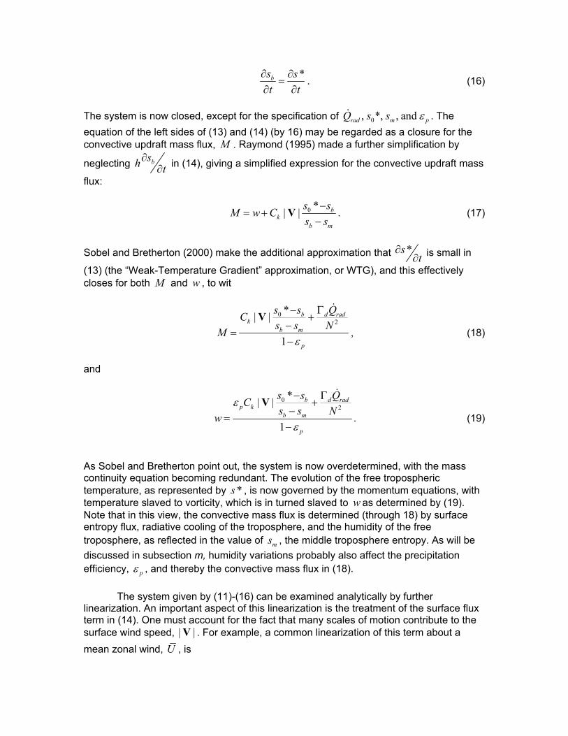
The system is now closed, except for the specification of 0, *, , andrad m pQ s s ε . The equation of the left sides of (13) and (14) (by 16) may be regarded as a closure for the convective updraft mass flux, M . Raymond (1995) made a further simplification by

neglecting bsh t∂

∂ in (14), giving a simplified expression for the convective updraft mass

flux:

0 *| | bk

b m

s sM w Cs s

−= +

−V . (17)

Sobel and Bretherton (2000) make the additional approximation that *s

t∂

∂ is small in

(13) (the “Weak-Temperature Gradient” approximation, or WTG), and this effectively closes for both M and w , to wit

02

*| |

1

b d radk

b m

p

s s QCs s NM

ε

− Γ+

−=

−

V, (18)

and

02

*| |

1

b d radp k

b m

p

s s QCs s Nw

ε

ε

− Γ+

−=

−

V. (19)

As Sobel and Bretherton point out, the system is now overdetermined, with the mass continuity equation becoming redundant. The evolution of the free tropospheric temperature, as represented by *s , is now governed by the momentum equations, with temperature slaved to vorticity, which is in turned slaved to w as determined by (19). Note that in this view, the convective mass flux is determined (through 18) by surface entropy flux, radiative cooling of the troposphere, and the humidity of the free troposphere, as reflected in the value of ms , the middle troposphere entropy. As will be discussed in subsection m, humidity variations probably also affect the precipitation efficiency, pε , and thereby the convective mass flux in (18). The system given by (11)-(16) can be examined analytically by further linearization. An important aspect of this linearization is the treatment of the surface flux term in (14). One must account for the fact that many scales of motion contribute to the surface wind speed, | |V . For example, a common linearization of this term about a mean zonal wind, U , is

2 2

*

| | ,U uU u+

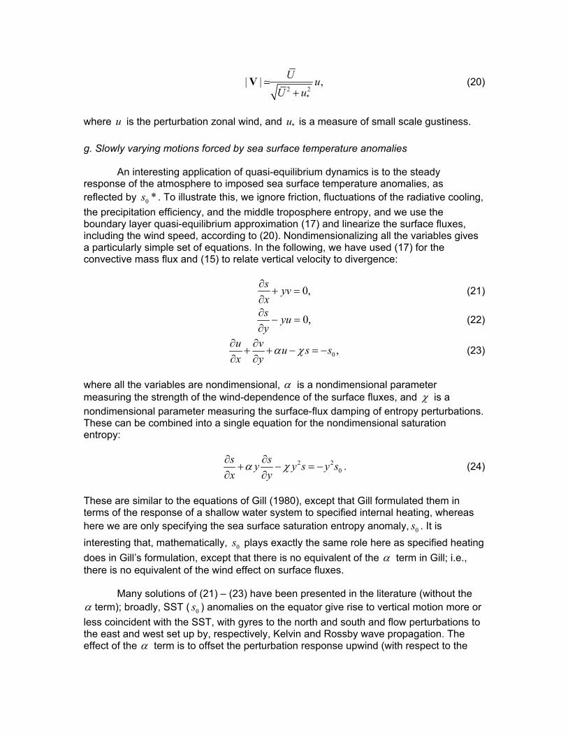
V (20)

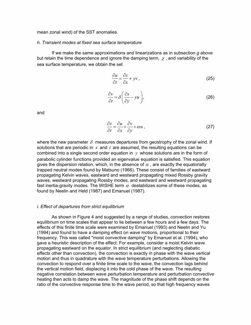
where u is the perturbation zonal wind, and *u is a measure of small scale gustiness. g. Slowly varying motions forced by sea surface temperature anomalies An interesting application of quasi-equilibrium dynamics is to the steady response of the atmosphere to imposed sea surface temperature anomalies, as reflected by 0 *s . To illustrate this, we ignore friction, fluctuations of the radiative cooling, the precipitation efficiency, and the middle troposphere entropy, and we use the boundary layer quasi-equilibrium approximation (17) and linearize the surface fluxes, including the wind speed, according to (20). Nondimensionalizing all the variables gives a particularly simple set of equations. In the following, we have used (17) for the convective mass flux and (15) to relate vertical velocity to divergence:

0,s yvx∂

+ =∂

(21)

0,s yuy∂

− =∂

(22)

0 ,u v u s sx y

α χ∂ ∂+ + − = −

∂ ∂ (23)

where all the variables are nondimensional, α is a nondimensional parameter measuring the strength of the wind-dependence of the surface fluxes, and χ is a nondimensional parameter measuring the surface-flux damping of entropy perturbations. These can be combined into a single equation for the nondimensional saturation entropy:

2 20

s sy y s y sx y

α χ∂ ∂+ − = −

∂ ∂. (24)

These are similar to the equations of Gill (1980), except that Gill formulated them in terms of the response of a shallow water system to specified internal heating, whereas here we are only specifying the sea surface saturation entropy anomaly, 0s . It is interesting that, mathematically, 0s plays exactly the same role here as specified heating does in Gill’s formulation, except that there is no equivalent of the α term in Gill; i.e., there is no equivalent of the wind effect on surface fluxes. Many solutions of (21) – (23) have been presented in the literature (without the α term); broadly, SST ( 0s ) anomalies on the equator give rise to vertical motion more or less coincident with the SST, with gyres to the north and south and flow perturbations to the east and west set up by, respectively, Kelvin and Rossby wave propagation. The effect of the α term is to offset the perturbation response upwind (with respect to the

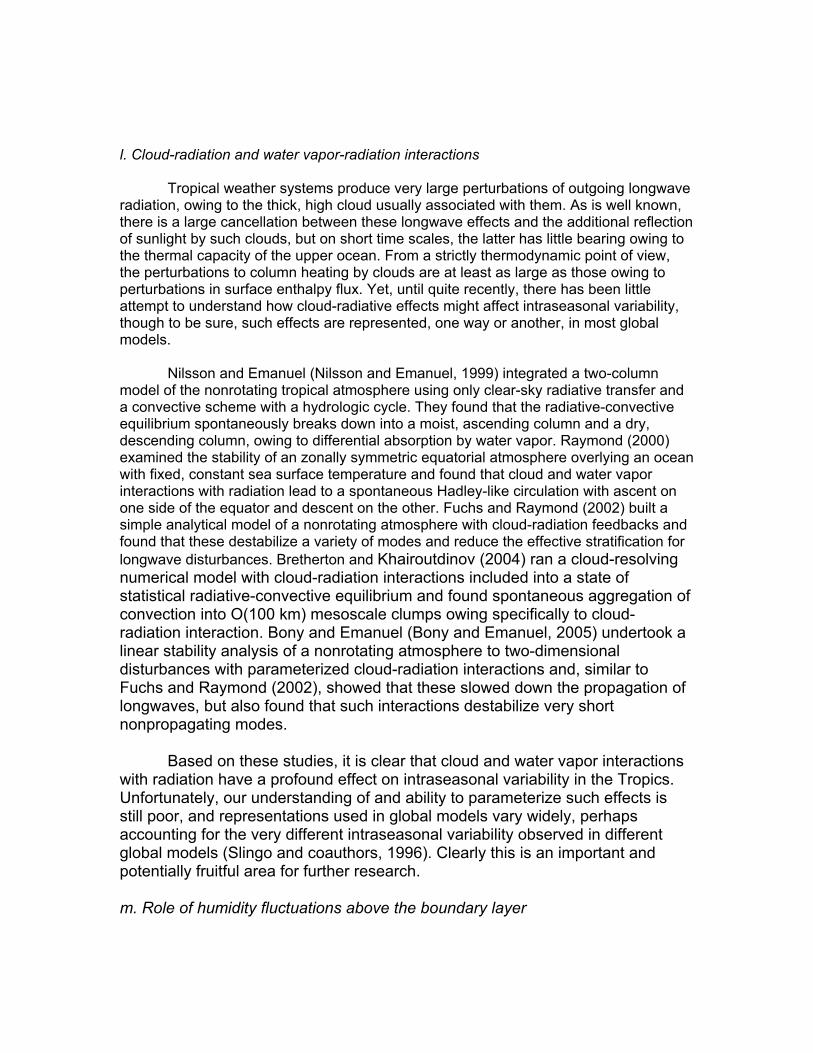
mean zonal wind) of the SST anomalies. h. Transient modes at fixed sea surface temperature If we make the same approximations and linearizations as in subsection g above but retain the time dependence and ignore the damping term, χ , and variability of the sea surface temperature, we obtain the set

u s yvt x

∂ ∂= +

∂ ∂, (25)

v s yut y

δ ∂ ∂

= − ∂ ∂ , (26)

and

s u v ut x y

α∂ ∂ ∂= + +

∂ ∂ ∂, (27)

where the new parameter δ measures departures from geostrophy of the zonal wind. If solutions that are periodic in x and t are assumed, the resulting equations can be combined into a single second order equation in y whose solutions are in the form of parabolic cylinder functions provided an eigenvalue equation is satisfied. This equation gives the dispersion relation, which, in the absence of α , are exactly the equatorially trapped neutral modes found by Matsuno (1966). These consist of families of eastward propagating Kelvin waves, eastward and westward propagating mixed Rossby gravity waves, westward propagating Rossby modes, and eastward and westward propagating fast inertia-gravity modes. The WISHE term α destabilizes some of these modes, as found by Neelin and Held (1987) and Emanuel (1987). i. Effect of departures from strict equilibrium As shown in Figure 4 and suggested by a range of studies, convection restores equilibrium on time scales that appear to lie between a few hours and a few days. The effects of this finite time scale were examined by Emanuel (1993) and Neelin and Yu (1994) and found to have a damping effect on wave motions, proportional to their frequency. This was called "moist convective damping" by Emanuel et al. (1994), who gave a heuristic description of the effect. For example, consider a moist Kelvin wave propagating eastward on the equator. In strict equilibrium (and neglecting diabatic effects other than convection), the convection is exactly in phase with the wave vertical motion and thus in quadrature with the wave temperature perturbations. Allowing the convection to respond over a finite time scale to the wave, the convection lags behind the vertical motion field, displacing it into the cold phase of the wave. The resulting negative correlation between wave perturbation temperature and perturbation convective heating then acts to damp the wave. The magnitude of the phase shift depends on the ratio of the convective response time to the wave period, so that high frequency waves

are preferentially damped. This may help explain the very red spectrum found in the Tropics (Wheeler and Kiladis, 1999). j. Taking the lid off The tropopause is not a physical barrier but represents a rather large change from the small effective stability of the tropical troposphere to the large stability of the stratosphere. The classical theory of (dry) equatorial waves may be supposed to apply in the stratosphere, and much work has been done on this topic, owing partially to the importance of upward propagating waves in driving the quasi-biennial oscillation of the equatorial stratosphere. In general, higher frequency waves also lose energy more rapidly to the stratosphere. Yano and Emanuel (1991) coupled a linear moist model of the tropical troposphere to a dry stratosphere, applying a wave radiation condition to the top, and showed that all but the lowest frequency moist waves of the troposphere are strongly damped by upward wave radiation. This is another effect that undoubtedly reddens the tropical tropospheric wave spectrum, but other than the above cited work, very little analytical research has been performed on this subject. k. WISHE It is important to note that in the statistical equilibrium theory of convection reviewed here, the interaction between large-scale circulations and convection per se is a stable one, leading the neutral or damped oscillatory solutions of linear equations that, when a rigid lid is applied at the tropopause, are mathematically identical to the shallow water equations. Observed circulations in the Tropics must therefore originate in stochastic forcing of the equatorial waveguide, in physical processes that serve to destabilize the oscillations, in externally forced gradients of the sea surface temperature, or in coupled instabilities of the ocean-atmosphere system.

One mechanism for internally destabilizing tropical perturbations takes advantage of the large reservoir of potential energy inherent in the thermodynamic disequilibrium that normally exists between the tropical oceans and atmosphere. (This disequilibrium is responsible for hurricanes, for example.) On reasonably short time scales, the ocean temperature may be assumed fixed, and fluctuations in the surface enthalpy flux will then be largely owing to fluctuations in near-surface wind speed. Neelin and Held (1987) and Emanuel (1987) showed that such an interaction, in the context of strict statistical equilibrium, destabilizes many of the moist equatorial modes, though their growth rates maximize at small scales. (Neelin and Held referred to this destabilization as “wind-evaporation feedback, while I have referred to it as “wind-induced surface heat exchange”, or WISHE.) Later work showed that either allowing wave radiation into the stratosphere (Yano and Emanuel, 1991) or accounting for the finite time scale of convection (Emanuel, 1993) damps the higher frequency modes, yielding maximum growth rates at synoptic to planetary scales. In particular, Emanuel (1993) showed that the surviving unstable modes are primarily planetary scale eastward-propagating Kelvin modes, eastward- and westward-propagating mixed Rossby-gravity modes, and westward-propagating Rossby modes. This is well in accord with the later findings of Wheeler and Kiladis (1999), analyzing space-time spectra of satellite-measured outgoing longwave radiation. Yet MJO-like modes are not among those predicted by WISHE theory.

l. Cloud-radiation and water vapor-radiation interactions Tropical weather systems produce very large perturbations of outgoing longwave radiation, owing to the thick, high cloud usually associated with them. As is well known, there is a large cancellation between these longwave effects and the additional reflection of sunlight by such clouds, but on short time scales, the latter has little bearing owing to the thermal capacity of the upper ocean. From a strictly thermodynamic point of view, the perturbations to column heating by clouds are at least as large as those owing to perturbations in surface enthalpy flux. Yet, until quite recently, there has been little attempt to understand how cloud-radiative effects might affect intraseasonal variability, though to be sure, such effects are represented, one way or another, in most global models. Nilsson and Emanuel (Nilsson and Emanuel, 1999) integrated a two-column model of the nonrotating tropical atmosphere using only clear-sky radiative transfer and a convective scheme with a hydrologic cycle. They found that the radiative-convective equilibrium spontaneously breaks down into a moist, ascending column and a dry, descending column, owing to differential absorption by water vapor. Raymond (2000) examined the stability of an zonally symmetric equatorial atmosphere overlying an ocean with fixed, constant sea surface temperature and found that cloud and water vapor interactions with radiation lead to a spontaneous Hadley-like circulation with ascent on one side of the equator and descent on the other. Fuchs and Raymond (2002) built a simple analytical model of a nonrotating atmosphere with cloud-radiation feedbacks and found that these destabilize a variety of modes and reduce the effective stratification for longwave disturbances. Bretherton and Khairoutdinov (2004) ran a cloud-resolving numerical model with cloud-radiation interactions included into a state of statistical radiative-convective equilibrium and found spontaneous aggregation of convection into O(100 km) mesoscale clumps owing specifically to cloud-radiation interaction. Bony and Emanuel (Bony and Emanuel, 2005) undertook a linear stability analysis of a nonrotating atmosphere to two-dimensional disturbances with parameterized cloud-radiation interactions and, similar to Fuchs and Raymond (2002), showed that these slowed down the propagation of longwaves, but also found that such interactions destabilize very short nonpropagating modes. Based on these studies, it is clear that cloud and water vapor interactions with radiation have a profound effect on intraseasonal variability in the Tropics. Unfortunately, our understanding of and ability to parameterize such effects is still poor, and representations used in global models vary widely, perhaps accounting for the very different intraseasonal variability observed in different global models (Slingo and coauthors, 1996). Clearly this is an important and potentially fruitful area for further research. m. Role of humidity fluctuations above the boundary layer

The quasi-equilibrium theory of tropical convection delineates a clear dependence of convection and large-scale ascent on the relative humidity of the lower and middle troposphere. Broadly, to balance a given surface enthalpy flux, there have to be more or stronger convective downdrafts if the entropy of the middle troposphere (the source region of the downdrafts) is higher, implying more convection. The WTG equations (18) and (19) make it clear that, all other things being equal, there will be more convection and more large-scale ascent in regions where the middle troposphere entropy, ms , is larger. Moreover, the precipitation efficiency ( pε ) is almost certainly a function of the relative humidity of the troposphere, being larger in a more humid atmosphere where less evaporation of precipitation occurs, and this works in the same direction. On the other hand, it is observed that ascending regions are generally more humid than regions where air is descending on the large scale, implying a possible feedback between mid-level moisture and convection. This feedback has come to be known as “moisture-convection” feedback and was perhaps first detected in the two-dimensional cloud-resolving simulations by Held et al. (1993). They found that when vertical wind shear is suppressed, moisture accumulates in one small region and the moist convection locks on to that region, being suppressed elsewhere. But modest amounts of shear disrupt the moisture anomaly and randomize the cloud field. Apparently, this feedback is not strong enough to organize moist convection in three dimensions…according to the work of Bretherton and Khairoutdinov (2004), self aggregation does not occur in the absence of cloud-radiative feedbacks. But Grabowski and Moncrieff (2004) find that that moisture-convection feedback is essential to obtain large-scale organization of convection in their aqua-planet, constant sea surface temperature model. Since moisture-convection feedback is sensitive to small scale processes such as turbulent entrainment and cloud microphysics, the magnitude of this effect is bound to depend on the nature of the model used. As in the case of cloud-radiation interaction, this is an area ripe for further research. n. Coupling to the ocean At time scales longer than a few days, the ocean cannot be considered to be an infinite heat capacitor and one must account for the energy budget of at least the ocean’s mixed layer. The tropical oceans exhibit substantial variability on intraseasonal time scales (Krishnamurti et al., 1988) and there is evidence that coupling to the ocean may be essential for explaining aspects of this variability (Sobel and Gildor, 2003; Maloney and Sobel, 2004). At even longer time scales, the dynamics of the ocean come into play, as for example with El Niño/Southern Oscillation. 4. Behavior of finite amplitude perturbations The quasi-linear theory of small perturbations to convective atmospheres, based on quasi-equilibrium ideas, may be expected to be approximately valid as long as the perturbations do not become so strong that deep convection is completely annihilated in certain regions. Once this happens, the convection-free regions are not constrained to be convectively neutral, and the physics that limits the strength of the circulations changes.

A simple model of the Walker Circulation, based on quasi-equilibrium and WTG,

suffices to illustrate some of issues involved. This model represents the circulation in terms of two boxes….one over relatively warm ocean and the other over relatively cold ocean, as illustrated in Figure 5. For simplicity, we take the boxes to have the same dimensions, and look for steady solutions to the QE WTG equations. There are two possible regimes: one in which deep convection occurs on both boxes (Figure 5a) and one in which deep convection is suppressed over the cold water (Figure 5b).

According to the postulate of convective neutrality, we insist on moist adiabatic

temperature lapse rates in both boxes in the first regime and over the warmer water in the second regime. But WTG also insists that there be no temperature gradient in the free troposphere between the two boxes. Taken together, these two postulates mean that we can represent the temperature in both boxes, in both regimes, as a single value of the saturation entropy, *s . Convective neutrality also stipulates the boundary layer entropy, bs , be equal to the saturation entropy of the free troposphere wherever there is deep convection. But in the second regime, the cold box does not contain deep convection and we allow bs to be lower than the free troposphere *s .

For simplicity, we omit WISHE, cloud-radiation and moisture-convection

feedbacks simply by taking | |DC constant=V ,

2d radQ R constantN

Γ≡ − = ,

p constantε = , and b ms s s constant− ≡ ∆ = . We then apply the WTG equations, (18) and (19), to each box of the first regime. Mass continuity demands that warm coldw w= − , and this condition, together with (18) and (19), determines the system saturation entropy, *s . It is convenient to replace the variables in this problem by nondimensional counterparts, according to

,1 p

Rw wε

→−

,1 p

RM Mε

→−

.| |D p

R ss sC ε

∆→

V

Then, in the first regime, where deep convection occurs in both boxes, the solutions for the single value of the entropy (which is the saturation entropy of both boxes and the boundary layer entropy of both boxes) and the vertical motion and convective mass fluxes in each box are

( )

( )

( )

( )

0 0

0 0

0 0

0 0

1 1,2

1 ,2

1 11 ,2

1 11 .2

w c

w c w c

w w cp p

c w cp p

s s s

w w s s

M s s

M s s

ε ε

ε ε

= + −

= − = −

= − + −

= − − −

Thus the system entropy is just the average of the saturation entropy of the sea surface in both boxes, minus a constant related to the radiative cooling of the troposphere. The large-scale circulation increases linearly with the imposed ocean saturation entropy difference, while the mass flux over the cold water decreases linearly with same. The mass flux over the cold water will decrease to zero when the saturation entropy difference between the two boxes exceeds the critical value ( )2 1 pε− . At that point, the solutions above are no longer viable and we must confront a different balance over the cold water. When deep convection is absent over the cold water, subsidence warming of the free troposphere must balance radiative cooling. In dimensional terms, this means that cw R= − . At the same time, the surface entropy flux in the cold box must be balanced by

the downward advection of low entropy from above the boundary layer…in dimensional

terms, ( )0| |D

c c cCw s ss

− = −∆

V. These two conditions determine the boundary layer

entropy of the cold box, cs . Since cs now differs from ws we have to allow for advection of entropy from the cold to the warm box. At the same time, the original WTG equations must apply in the warm box, modified by the horizontal entropy advection, and of course, warm coldw w= − . Using the same nondimensionalizations as before, the solution in this

regime is given by (1 ),c w pw w ε= − = − −

0c c ps s ε= − ,

( )0 02

* ,1

w p c pw

s ss s

ε χ εχ

+ − + −= =

+

( )2 1 p

wp

Mε

ε

−= ,

0,cM = where | |k

RCχ ≡ V . (This measures the relative strength of horizontal entropy

advection.) Clearly, the circulation no longer increases with increasing sea surface

temperature difference in this regime: the magnitude of the circulation is absolutely limited by the radiative cooling over the cold water. Reducing the temperature of the cold water reduces both the system entropy and the boundary layer entropy over the cold water, but does not affect the circulation strength. In the real word, though, the relative areas covered by the deep convection and no convection regimes are free to vary, and so there may be additional increases in the strength of the circulation with increasing SST gradient. Bretherton and Sobel (2002) took this into account in a similar model of the Walker Circulation, but one which is horizontally continuous. They also showed that the interaction between low clouds and radiation is an important effect in such circulations.

Quantitatively, it takes little sea surface temperature gradient to shut off deep

convection over the colder water. Once this happens, the magnitude of the circulation becomes rate-limited by the amount of radiational cooling that can occur in the dry regions.

The fact that most tropical circulations are strong enough to shut off deep

convection in various regions perhaps limits the utility of the theory of linear perturbations to radiative convective equilibrium states, though it does not, in and of itself, invalidate the notion of quasi-equilibrium. But it does mean that the separation between moist ascending regions and dry subsiding regions, on a large scale, is an important and irreducibly nonlinear aspect of many tropical circulation systems.

A possible exception to this conclusion is the case of tropical cyclones. The

existing theory (see Emanuel (2003) for a review) shows that the intensity of the circulation is limited by surface fluxes in the high wind core near the eyewall with no rate-limiting role played by the broad descent outside the core. This is no doubt owing to the circular geometry of these storms, which allows for broad outer regions of descent to compensate for a narrow, intense plume of ascent at the core. 5. Some examples of the application of quasi-equilibrium closure To illustrate the power of quasi-equilibrium, I here show two rather different examples of the application of quasi-equilibrium dynamics to the tropical atmosphere. The first is a simple model of the equatorial beta plane on an aqua planet, and the second is to the real time prediction of hurricane intensity. a. A simple quasi-equilibrium model of the equatorial waveguide

This model simply integrates the first baroclinic mode equations (11) - (15), ignoring any contribution for the barotropic mode. (For this reason, it effectively assumes a rigid lid and ignores the coupling of baroclinic and barotropic motions through surface friction or nonlinearity.) An equilibrium convective updraft mass flux is defined using boundary layer QE, according to (17), and the actual convective updraft mass is relaxed toward this equilibrium value over a finite time, to allow for the effects of nonzero convective response time, as discussed in section 3i. Cloud-radiation interactions are parameterized as a function of the middle troposphere relative humidity, following Bony and Emanuel (2005), and the precipitation efficiency is also function of the mid-troposphere relative humidity. The model is run in an equatorially centered channel, from 40o S to 40o N, with only 42 grid points in each direction. For the simulations presented here, the underlying sea surface temperature is specified as a zonally symmetric profile with a broad, flat peak at the equator. Figure 6 shows the equatorially symmetric and asymmetric power spectra of the vertical velocity averaged over 200 days. On these plots, positive zonal wavenumbers correspond to eastward propagation, while negative wavenumbers show westward propagation. The plot of the symmetric component (Figure 6a) shows a prominent Kelvin wave signal corresponding to eastward propagation at about 120 ms− , while the asymmetric component (Figure 6b) shows a mixed Rossby-gravity signal. Power spectra of the asymmetric meridional wind (not shown) also display a prominent planetary Rossby modes. These diagrams are quite similar to the power spectra of outgoing longwave radiation produced by Wheeler and Kiladis (1999), but the Madden-Julian Oscillation (MJO) is notably absent. The variability evident in Figure 6 is caused in the model mostly by WISHE and cloud-radiation interactions. b. Tropical cyclones In some ways, the inner core of a tropical cyclone provides a severe test for quasi-equilibrium. The intrinsic dynamical space and time scales of the inner core are

related to the eye diameter and the rotational frequency max

max

vr , the ratio of the

maximum tangential wind to the radius of maximum winds. These space and time scales are not very different from those associated with cumulonimbus clouds, and so one should be concerned whether the convection ever approaches statistical equilibrium with the cyclone. Nevertheless, a simple model based on quasi-equilibrium simulates actual tropical cyclones well enough that it is used as a forecasting aid by operational prediction centers. The model in question is called the Coupled Hurricane Intensity Prediction System (CHIPS) and is described in detail in Emanuel et al. (2004). Quasi-equilibrium is implemented in this model by assuming that the free tropospheric temperature lapse rate is always moist adiabatic on surfaces of constant absolute angular momentum about the storm’s central axis. This is tantamount to assuming that in a strongly baroclinic environment, such as the eyewall of a hurricane, slantwise (rather than upright) convective neutrality is maintained. No first-baroclinic-mode assumption is made; instead, angular momentum conservation is invoked at the tropopause as an additional constraint, and the partitioning between first baroclinic and barotropic modes is made naturally by the model itself. As in the equatorial wave guide model described in the previous subsection, relaxed boundary layer quasi-equilibrium is employed, although in

this case it is necessary to account for horizontal entropy advection within the boundary layer. In the limiting case of a tropical cyclone reaching its potential intensity, the surface entropy flux is balanced by radial advection of entropy rather than by import of low entropy by convective downdrafts. Figure 7 shows a hindcast of a particular Atlantic hurricane. The hindcast has the advantage that the actual track is known, and the environmental shear is better known than in a forecast. The model does a good job simulating the intensity evolution of this and other events. This suggest that the assumption of quasi-equilibrium is, at any rate, not a terribly bad one even in a hurricane. 6. Summary and concluding thoughts Moist convection plays an important role in many and perhaps most tropical circulation systems. Convection itself is a deeply chaotic phenomenon with space scales of meters to kilometers and time scales of second to hours. On the other hand, the space and time scales of many tropical circulations systems are substantially larger, offering the hope that the fast, small-scale convective processes may be regarded as approximately in statistical equilibrium with the slower and bigger tropical circulations. In this review I discussed one popular rendition of statistical equilibrium in which it is assumed that convection maintains moist adiabatic lapse rates and the neutral stability of the tropical troposphere with respect to adiabatically lifted air from the subcloud layer. This is not the only form of statistical equilibrium that has been tried, nor is it necessarily the best, but it does seem to work well for a variety of phenomena, even including tropical cyclones. As pointed out by Arakawa and Schubert (1974), statistical equilibrium is a precondition for parameterization. Without some kind of equilibrium or near-equilibrium assumption, the collectively effects of a small scale process cannot be uniquely related to large-scale variables. Of course, convection in the real world may not be characterized as nearly in statistical equilibrium, at least in certain places at certain times. One of the supposed benefits of simulating the tropical atmosphere with convection-resolving models is the ability to do away with convective parameterization and all the baggage it carries, including the assumption of equilibrium. But it is important to be clear about this. To the extent that statistical equilibrium does not exist, then more than one realization of convection may occur for the same large scale flow. If the feedback of convection on the large scale is important, this means that there may be more than one (and perhaps many) large-scale tendencies for exactly the same large-scale realization. Fundamentally, this means that the high frequency chaos of small scale convection is immediately felt at the large scale, and one must then confront a basic predictability problem. Explicitly resolving the unpredictable small scale convection buys one nothing unless one is prepared to run large ensembles. Resolving the unpredictable is not obviously preferable to predicting the unresolvable. In its current state of development, the statistical equilibrium theory of moist convection makes certain testable predictions about tropical dynamics. First, it predicts that the available potential energy inherent in the vertically unstable stratification of the

tropical atmosphere is not available to power large-scale disturbances. Indeed, the simple rendition of equilibrium as enforcing moist adiabatic lapse rates and boundary layer quasi-equilibrium predicts that large scale motions will be damped by their interaction with convection. Observed tropical atmospheric phenomena would then have to be powered by one or more of the following:

• Sea surface temperature gradients • Energy propagation into the Tropics from higher latitudes • WISHE • Cloud and moisture interactions with radiation • Feedbacks involving convection and middle tropospheric moisture • Feedbacks involving the ocean and/or land surfaces

Simple models based on statistical equilibrium postulates appear to be successful in explaining basic aspects of many tropical phenomena, ranging from tropical cyclones to the Walker circulation. On the other hand, no generally accepted paradigm for the Madden-Julian Oscillation has emerged, though there is no shortage of candidates. Among the many tropical processes that could profit from a better theoretical understanding are

• Coupling of the first baroclinic and barotropic modes, through surface friction and through wave radiation into the stratosphere

• The possible role of the second and higher baroclinic modes • The effects of convective momentum transfer • Cloud and moisture interactions with radiation • The effect of mid-level moisture on convection

As advancing computer power begins to allow us to resolve convective clouds and large-scale circulations simultaneously, it will become possible to rigorously test the quasi-equilibrium postulate, to refine our understanding of some of the processes mentioned above, and also to build better representations of those processes to run in faster and cheaper models.

References Arakawa, A. and W. H. Schubert, 1974: Interaction of a cumulus cloud ensemble with

the large-scale environment, Part I. J. Atmos. Sci., 31, 674-701 Betts, A. K., 1986: A new convective adjustment scheme. Part I: Observational and

theoretical basis. Quart. J. Roy. Meteor. Soc., 112, 677-691. Bjerknes, J., 1938: Saturated-adiabatic ascent of air through dry-adiabatically

descending environment. Quart. J. Roy. Meteor. Soc., 64, 325-330. Bony, S. and K. Emanuel, 2005: On the role of moist processes in tropical intraseasonal

variability: cloud-radiation and moisture-convection feedbacks. J. Atmos. Sci., 62, in press

Bretherton, C. S. and M. F. Khairoutdinov, 2004: Convective self-aggregation in large

cloud-resolving model simulations of radiative convective equilibrium. AMS Conference on Hurricanes and Tropical Meteorology, Miami, Amer. Meteor. Soc.

Bretherton, C. S. and A. H. Sobel, 2002: A simple model of a convectively coupled

Walker Circulation using the weak temperature gradient approximation. J. Climate, 15, 2907-2920

Brown, R. G. and a. C. S. Bretherton, 1995: Tropical wave instabilities. J. Atmos.. Sci.,

51, 67-82. Deardorff, J. W., 1972: Numerical investigation of neutral and unstable planetary

boundary layers. J. Atmos.. Sci., 29, 91-115. Emanuel, K., 2003: Tropical cyclones. Ann. Rev. Earth Plan. Sci., 31, 75-104 Emanuel, K., C. DesAutels, C. Holloway and R. Korty, 2004: Environmental control of

tropical cyclone intensity. J. Atmos. Sci., 61, 843-858 Emanuel, K. A., 1987: An air-sea interaction model of intraseasonal oscillations in the

tropics. J. Atmos.. Sci., 44, 2324-2340. ______, 1993: The effect of convective response time on WISHE modes. J. Atmos.. Sci.,

50, 1763-1775 ______, 1994: Atmospheric Convection. Oxford Univ. Press, New York, 580 pp. pp Emanuel, K. A. and M. Živkovic-Rothman, 1999: Development and evaluation of a

convection scheme for use in climate models. J. Atmos. Sci., 56, 1766-1782 Emanuel, K. A., J. D. Neelin and C. S. Bretherton, 1994: On large-scale circulations in

convecting atmospheres. Quart. J. Roy. Meteor. Soc., 120, 1111-1143 Fuchs and D. J. Raymond, 2002: Large-scale modes of a nonrotating atmosphere with

water vapor and cloud–radiation feedbacks. J. Atmos. Sci., 59, 1669-1679 Gill, A. E., 1980: Some simple solutions for heat-induced tropical circulation. Quart. J.

Roy. Meteor. Soc., 106, 447-462 Grabowski, W. W. and M. W. Moncrieff, 2004: Moisture-convection feedback in the

tropics. Quart. J. Roy. Meteor. Soc., 130, 3081-3104 Held, I. M., R. S. Hemler and V. Ramaswamy, 1993: Radiative-convective equilibrium

with explicit two-dimensional moist convection. J. Atmos. Sci., 50, 3909-3927 Islam, S., R. L. Bras and K. Emanuel, 1993: Predictability of mesoscale rainfall in the

tropics. J. Appl. Meteor., 32, 297-310 Krishnamurti, T. N., D. K. Oosterhof and A. V. Mehta, 1988: Air–sea interaction on the

timescale of 30 to 50 days. J. Atmos. Sci., 45, 1304-1322

Maloney, E. D. and A. H. Sobel, 2004: Surface fluxes and ocean coupling in the tropical

intraseasonal oscillation. J. Climate, 17, 4368-4386 Matsuno, T., 1966: Quasi-geostrophic motions in the equatorial area. J. Meteor. Soc.

Japan, 44, 25-42 Morton, B. R., G. I. Taylor, and J. S. Turner, 1956: Turbulent gravitational convection

from maintained and instantaneous sources. Proc. Roy. Soc. London, A234, 1-23

Neelin, J. D. and a. K. H. C. I. M. Held, 1987: Evaporation-wind feedback and low-

frequency variability in the tropical atmosphere. J. Atmos.. Sci., 44, 2341-2348. Neelin, J. D. and J. Yu, 1994: Modes of tropical variability under convective adjustment

and the Madden-Julian oscillation. Part I: Analytical theory. J. Atmos. Sci., 51, 1876-1894

Nilsson, J. and K. A. Emanuel, 1999: Equilibrium atmospheres of a two-column radiative

convective model. Quart. J. Roy. Meteor. Soc., 125, 2239-2264 Paluch, I. R., 1979: The entrainment mechanism in Colorado cumuli. J. Atmos. Sci., 36,

2462-2478 Pauluis, O. and I. M. Held, 2002: Entropy budget of an atmosphere in radiative-

convective equilibrium. Part I: Maximum work and frictional dissipation. J. Atmos. Sci., 59, 125-139

Prandtl, L., 1942: Fürher durch die Strömungslehre. Braunschweigh Vieweg und Sohn,

407 pp [English translation: Prandtl, L., 1952: Essentials of Fluid Dynamics. Hafner, 452 pp.]

Raymond, D. J., 1995: Regulation of moist convection over the west Pacific warm pool.

J. Atmos. Sci., 52, 3945-3959 ______, 2000: The Hadley circulation as a radiative–convective instability. J. Atmos.

Sci., 57, 1286-1297 Reed, R. J. and E. E. Recker, 1971: Structure and properties of synoptic-scale wave

disturbances in the equatorial western Pacific. J. Atmos. Sci., 28, 1117-1133. Robe, F. R. and K. Emanuel, 1996: Dependence of tropical convection on radiative

forcing. J. Atmos. Sci., 53, 3265-3275 Slingo, J. M. and coauthors, 1996: Intraseasonal oscillations in 15 atmospheric general

circulation models: results from an AMIP diagnostic subproject. Clim. Dyn., 12, 325-357

Sobel, A. H. and C. S. Bretherton, 2000: Modeling tropical precipitation in a single

column. J. of Climate, 13, 4378-4392

Sobel, A. H. and H. Gildor, 2003: A simple time-dependent model of SST hot spots. J. Climate, 16, 3978-3992

Warner, J., 1970: On steady state one-dimensional models of cumulus convection. J.

Atmos. Sci., 27, 1035-1040 Wheeler, M. and G. N. Kiladis, 1999: Convectively coupled equatorial waves: Analysis of

clouds and temperature in the wavenumber-frequency domain. J. Atmos. Sci., 56, 374-399

Xu, K.-M. and a. K. A. Emanuel, 1989: Is the tropical atmosphere conditionally unstable?

Mon. Wea. Rev., 117, 1471-1479 Yano, J.-I. and a. K. A. Emanuel, 1991: An improved WISHE model of the equatorial

atmosphere and its coupling with the stratosphere. J. Atmos. Sci., 48, 377-389 Yano, J.-I., J. C. McWilliams, M. W. Moncrieff and K. Emanuel, 1995: Hierarchical

tropical cloud systems in an analog shallow-water model. J. Atmos. Sci., 52, 1723-1742

Figure Captions 1. Contour plot of the difference between the environmental density temperature and the density temperature of a parcel lifted reversibly and adiabatically from the pressure level given on the abscissa to the pressure level on the ordinate. This quantity has been averaged over several thousand soundings taken at Kapingamarangi in the tropical western South Pacific. 2. 2-day running mean of the density temperature averaged between 900 and 200 hPa, and a 10-day running mean of the density temperature of a sample lifted reversibly from 940 hPa, also averaged between 900 and 200 hPa. The time series at Kapingamarangi runs from 1 July 1992 to 30 June 1993. 3. 2-day running mean of the density temperature averaged between 900 and 500 hPa (solid) and between 545 and 200 hPa (dashed); an offset of 34 K has been added to the latter. The time series at Kapingamarangi runs from 1 July 1992 to 30 June 1993. 4. Evolution with time of the vertical profile of perturbation temperature in a single-column model in which the initial temperature has been perturbed away from equilibrium by a maximum of 3 K, centered at 450 hPa. 5. Illustrating the two regimes of a two-box model of the Walker circulation. In (a), deep convection is assumed to occur in both boxes, while in (b) it is assumed to occur only over the warmer water, at left. The saturation entropy (i.e. the temperature) of the ocean surface is specified as 0ws for the warm column at left, and 0cs for the cold column at right. The free troposphere temperature in the warm box is assumed to lie along a moist adiabat, so that the saturation entropy, *s , is constant with height; the weak temperature gradient (WTG) approximation holds that the free troposphere temperature (and therefore *s ) must be the same over the cold water. In the warm regime, convective neutrality specifies that the boundary layer entropy, bs must equal the saturation entropy of the overlying troposphere in both boxes, but in the cold regimes, the boundary layer entropy in the cold box, bcs is less than *s , signifying stability to deep moist convection. 6. Frequency-wavenumber power spectra of the equatorially symmetric (a) and asymmetric (b) parts of the vertical velocity averaged over a 120-day integration of an equatorial channel model in which the troposphere is assumed to have a moist adiabatic lapse rate, only the first baroclinic mode is retained, and convection is represented according to a relaxed version of boundary layer quasi-equilibrium. Positive wavenumbers indicate eastward wave propagation. 7. Hindcast of the evolution with time of the maximum surface winds in Atlantic Hurricane Charley of 2004 (dashed) compared to estimates from observations (solid). The simulation was done using the Coupled Hurricane Intensity Prediction System (CHIPS), a model that uses a simple quasi-equilibrium convection scheme. The hindcast uses the actual track of the hurricane to estimate environmental conditions.

Figure 1

Figure 2

Figure 3

Figure 4

(a)

(b)

Figure 5

Figure 6

(a)

(b)

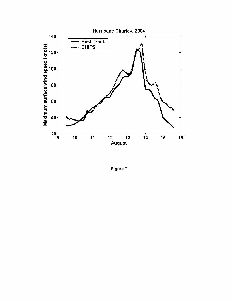
Figure 7