quasi-equilibrium theory of small perturbations to...
TRANSCRIPT

Quasi-equilibrium Theory of Small Perturbations to Radiative-
Convective Equilibrium States• See “CalTech 2005” paper on web site• Free troposphere assumed to have moist
adiabatic lapse rate (s* does not vary with height
• Boundary layer quasi-equilibrium applies

Basis of statistical equilibrium physics
• Dates to Arakawa and Schubert (1974)• Analogy to continuum hypothesis:
Perturbations must have space scales >> intercloud spacing
• TKE consumption by convection ~ CAPE generation by large scale
• Numerical models on the verge of simulating clouds + large-scale waves
• We further assume convective criticality

Implications of the moist adiabatic lapse rate for the structure of
tropical disturbances• Approximate moist adiabatic condition as
that of constant saturation entropy:
• Assume hydrostatic perturbations:0 0
** ln ln vp d
L qpTs c RT p T⎛ ⎞ ⎛ ⎞= − +⎜ ⎟ ⎜ ⎟⎝ ⎠ ⎝ ⎠
' 'pφ α∂
= −∂

• Maxwell’s relation:
• Integrate:
*
' * ' * '* p s
Ts ss pαα
⎛ ⎞∂ ∂⎛ ⎞= = ⎜ ⎟⎜ ⎟∂ ∂⎝ ⎠ ⎝ ⎠
( )' '( , , ) ( , , ) * 'b x y t T x y t T sφ φ= + −
Only barotropic and first baroclinic mode survive
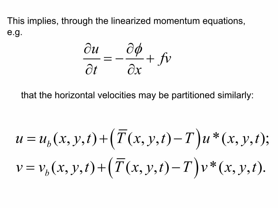
This implies, through the linearized momentum equations, e.g.
u fvt x
φ∂ ∂= − +
∂ ∂
that the horizontal velocities may be partitioned similarly:
( )( )
( , , ) ( , , ) *( , , );
( , , ) ( , , ) *( , , ).b
b
u u x y t T x y t T u x y t
v v x y t T x y t T v x y t
= + −
= + −


Implications for vertical structure of vertical velocity
u vp x yω ⎛ ⎞∂ ∂ ∂= − +⎜ ⎟∂ ∂ ∂⎝ ⎠
Integrate:
( ) ( )( )0
0 0* *' .
pb bp
u v u vp p p p T Tdpx y x y
ω⎛ ⎞ ⎛ ⎞∂ ∂ ∂ ∂
= − + − − − +⎜ ⎟ ⎜ ⎟∂ ∂ ∂ ∂⎝ ⎠ ⎝ ⎠∫
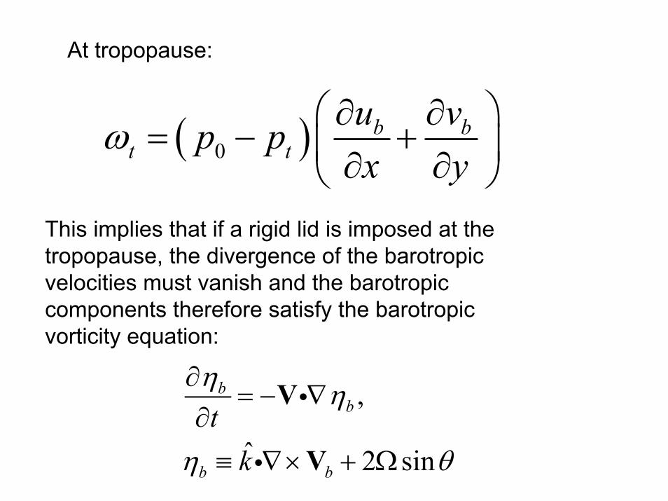
At tropopause:
( )0b b
t tu vp px y
ω⎛ ⎞∂ ∂
= − +⎜ ⎟∂ ∂⎝ ⎠This implies that if a rigid lid is imposed at the tropopause, the divergence of the barotropicvelocities must vanish and the barotropiccomponents therefore satisfy the barotropicvorticity equation:
,
ˆ 2 sin
bb
b b
tk
η η
η θ
∂= − ∇
∂≡ ∇× + Ω
V
V
i
i

Feedback of Air Motion on (virtual) Temperature
• Convection cannot change vertically integrated enthalpy,
• The neglecting surface fluxes, radiation, and horizontal advection,
• Neelin and Held (1987): This function is negative for upward motion
p vk c T L q= +
,hkdp dpt p
ω∂ ∂= −
∂ ∂∫ ∫
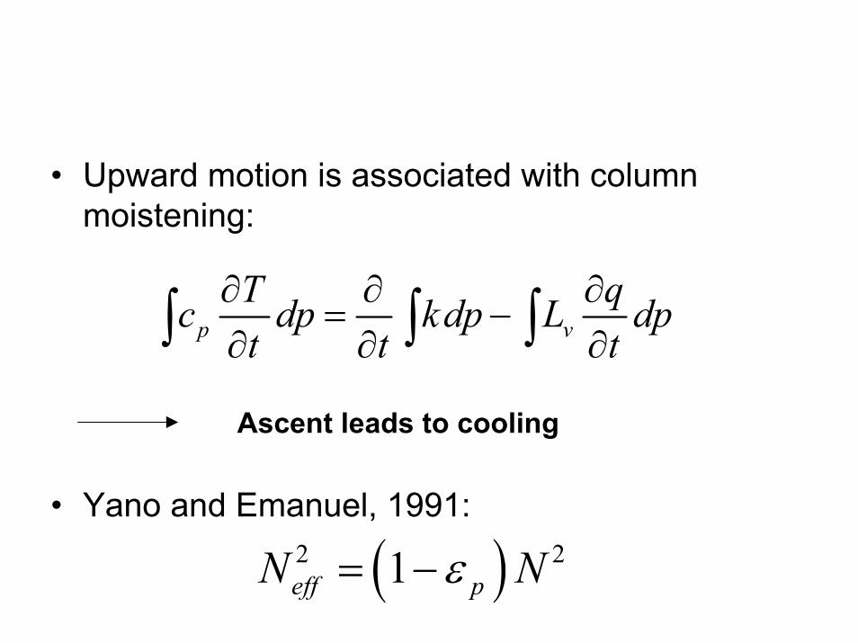
• Upward motion is associated with column moistening:
• Yano and Emanuel, 1991:
p vT qc dp kdp L dpt t t
∂ ∂ ∂= −
∂ ∂ ∂∫ ∫ ∫
Ascent leads to cooling
( )2 21eff pN Nε= −

Prediction: Inviscid, small amplitude perturbations under rigid lid: Shallow water solutions with reduced equivalent depth

Quasi-Linear Plane System , Neglecting Barotropic Mode
β
( ) *s
u sT T yv rut x
β∂ ∂= − + −
∂ ∂
( ) *s
v sT T yu rvt y
β∂ ∂= − − −
∂ ∂
( )* d drad p
m
ss Q M wt z
εΓ ∂∂ ⎛ ⎞= + −⎜ ⎟∂ Γ ∂⎝ ⎠&
( ) ( )( )0| | *bk b b m
sh C s s M w s st
∂= − − − −
∂V
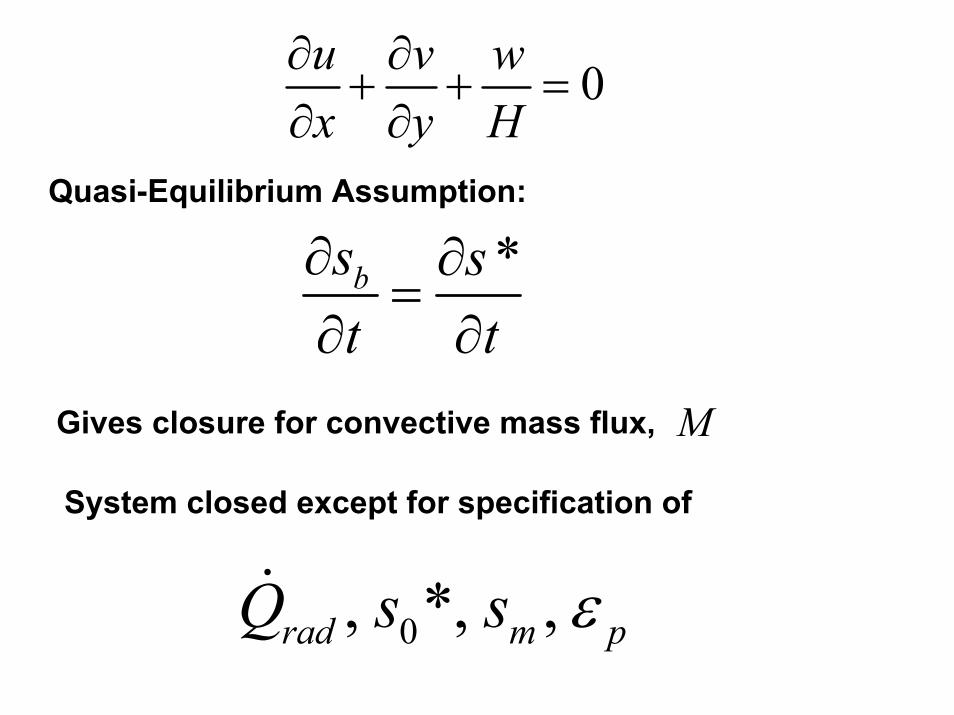
0u v wx y H∂ ∂
+ + =∂ ∂
Quasi-Equilibrium Assumption:
*bs st t
∂ ∂=
∂ ∂Gives closure for convective mass flux, M
System closed except for specification of
0, *, ,rad m pQ s s ε&

Additional Approximations:
• Boundary Layer QE (Raymond, 1995): Neglect , gives simpler expression for
• Weak Temperature Approximation(Sobel and Bretherton, 2000): Neglect (Over-determined system, ignore momentum equation for irrotational flow)
bsh t∂
∂M
*st
∂∂
0 *| | bk
b m
s sM w Cs s
−= +
−V

Important Feedbacks:
• Wind-Induced Surface Heat Exchange(WISHE) Coupling of surface enthalpy flux to wind perturbations (Neelin et al. 1987, Emanuel, 1987)
• Moisture-Convection Feedback: Dependence of on and/or on
• Cloud-Radiation Feedback: Dependence of on or
ms pεM * ms s−
radQ& M * ms s−

• Ocean-Atmosphere Feedback (e.g. ENSO): Feedback between perturbation surface wind and ocean surface temperature, as represented by 0 *s

Simple Example:• Ignore perturbations of• Ignore fluctuations of • Make boundary layer QE approximation • Fully linearize surface fluxes:
radQ&pε
2 2| | *U u= +V
'| | '| |Uu
=VV

Introduce scalings:
:yLFirst define a merdional scale,
( )42
1 pd dy s
m
sL T T Hz
εβ−Γ ∂
= −Γ ∂
Then let
( )
2
2
| |
| | | |* *
y
k
y
y k k y
s
x a x y L y
aCat t u uL H
L C aC Lv v s s
H H T T
β
β
→ →
→ →
→ →−
V
V V

Separate scalings for ocean temperature and lower tropospheric entropy:
( )
( )( )
0
2
0
1*
1
* *
po b m
p
b mpm m
p
s s s s
s ss s
s s
εε
εε
−→ −
−−→
−

Nondimensional parameters:
( )( )
( )( )( )
0
2
20
2
2
* *1( )
| | *
( )
* *1 | |( )
*
( )
p k
p m
y
p k y
p s m
y
s saC U WISHEH s s
ra Rayleigh frictionL
s saC Lsurface damping
H T T s s
a zonal geostropyL
εα
ε
β
ε βχ
ε
δ
−−≡
−
≡
−−≡
− −
⎛ ⎞= ⎜ ⎟⎜ ⎟⎝ ⎠
V
V
R

Nondimensional Equations:
u s yv ut x
∂ ∂= + −
∂ ∂R
v s yu vt y
δ⎛ ⎞∂ ∂
= − −⎜ ⎟∂ ∂⎝ ⎠R
0 ms u v u s s st x y
α χ∂ ∂ ∂= + + + + −
∂ ∂ ∂
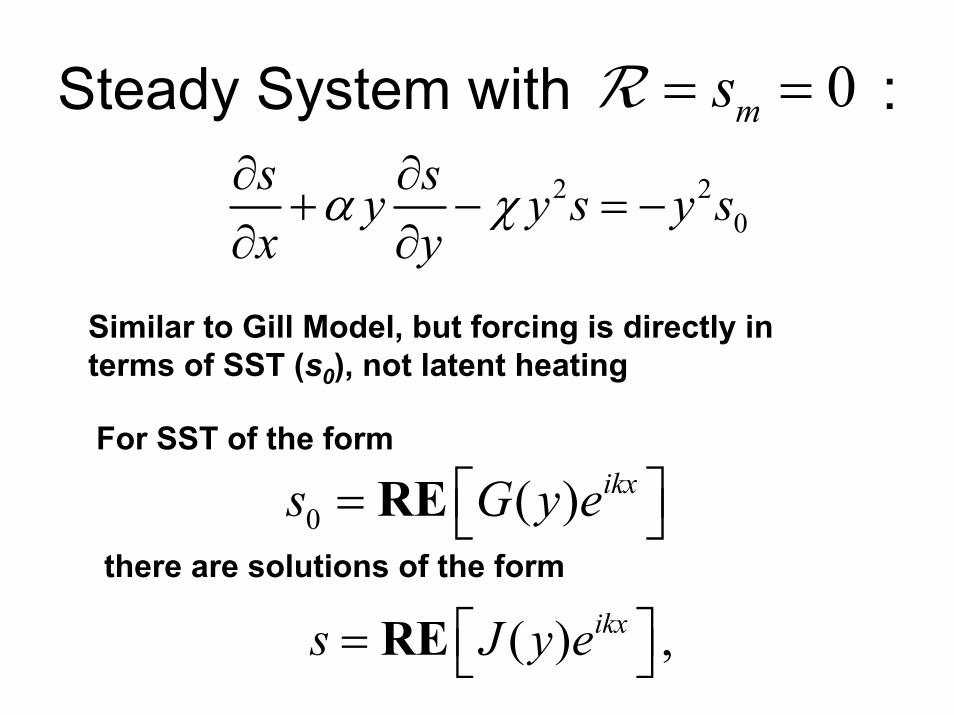
Steady System with : 0ms= =R2 2
0s sy y s y sx y
α χ∂ ∂+ − = −
∂ ∂
Similar to Gill Model, but forcing is directly in terms of SST (s0), not latent heating
For SST of the form
0 ( ) ikxs G y e⎡ ⎤= ⎣ ⎦REthere are solutions of the form
( ) ,ikxs J y e⎡ ⎤= ⎣ ⎦RE
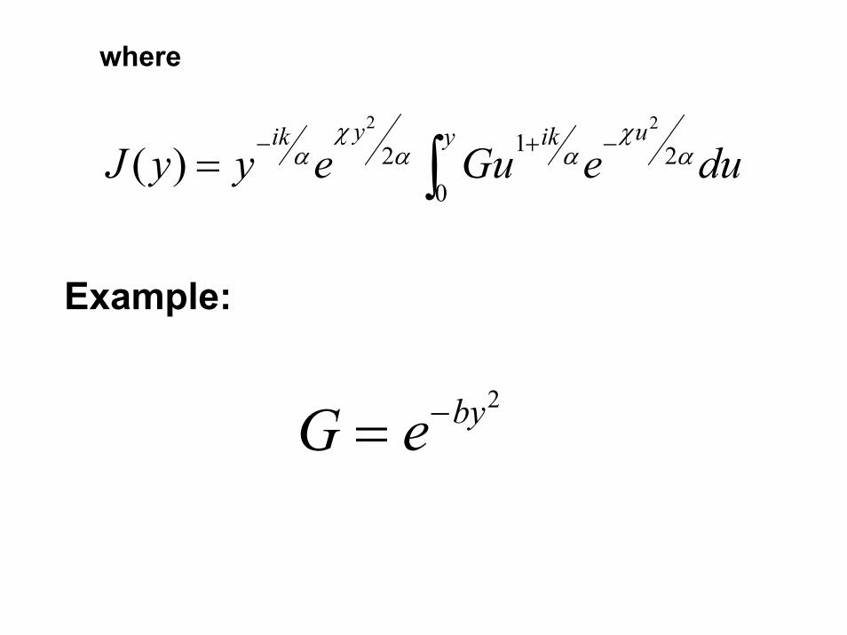
where
2 212 2
0( )
y uik ikyJ y y e Gu e du
χ χα α α α− + −= ∫
Example:
2byG e−=
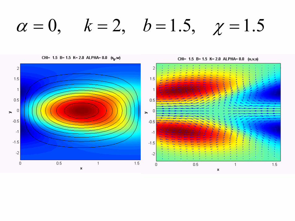
0, 2, 1.5, 1.5k bα χ= = = =

1, 2, 1.5, 1.5k bα χ= − = = =
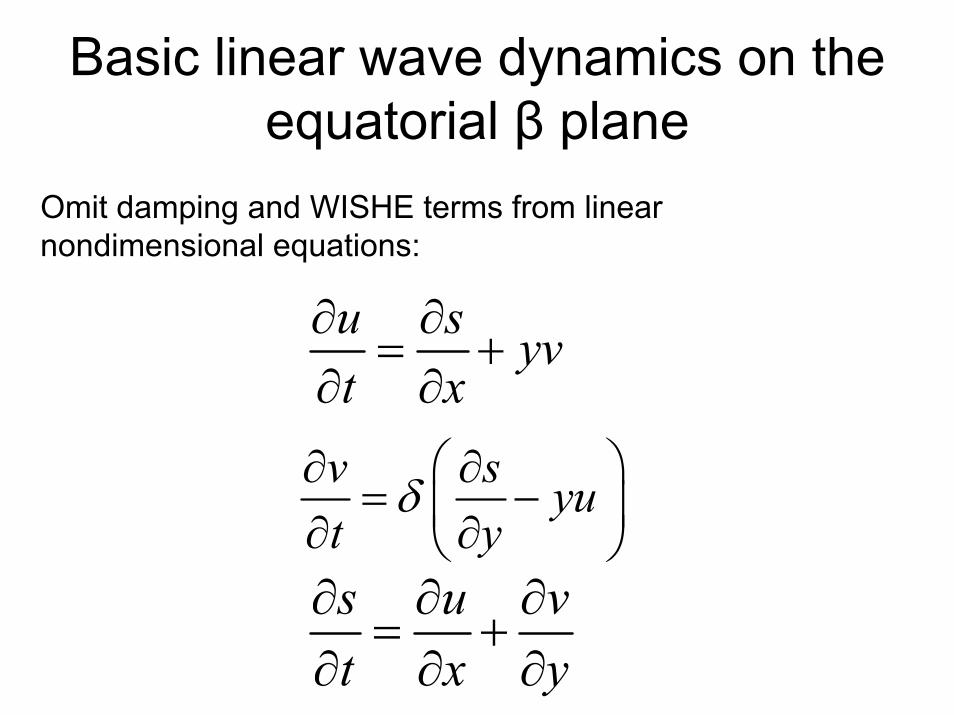
Basic linear wave dynamics on the equatorial β plane
Omit damping and WISHE terms from linear nondimensional equations:
u s yvt x
∂ ∂= +
∂ ∂
v s yut y
δ⎛ ⎞∂ ∂
= −⎜ ⎟∂ ∂⎝ ⎠s u vt x y∂ ∂ ∂
= +∂ ∂ ∂

Fully equivalent to the shallow water equations on a β plane
Eliminate s and u in favor of v:
2 2 22
2 2 2 0v v v vy vt t x y x
δ δ δ⎧ ⎫∂ ∂ ∂ ∂ ∂
− − + − =⎨ ⎬∂ ∂ ∂ ∂ ∂⎩ ⎭
( ) ikx i tv V y e ω−=Let
2 2 22
2 0d V k k y Vdy
ωδ ω
⎛ ⎞−→ + − − =⎜ ⎟
⎝ ⎠

y→±∞Boundary conditions: V well behaved at
:nDSolution in terms of discrete parabolic cylinder functions
22 2
( ),
1, 2 , 4 2,n
yn
v D y
where D e y y−
=
⎡ ⎤= −⎣ ⎦K
provided ω satisfies the dispersion relation
2 2
2 1k k nωδ ω−
− = +

There is, in addition, another mode satisfying v=0 everywhere. From first and third linear equations:
( )
2 2
2 2 0.
.
u ut xSatisfied by u F x t
∂ ∂− =
∂ ∂= −
Eastward-propagating, nondispersiveequatorially trapped Kelvin wave
Note that this happens to satisfy derived dispersion relation when n= -1.
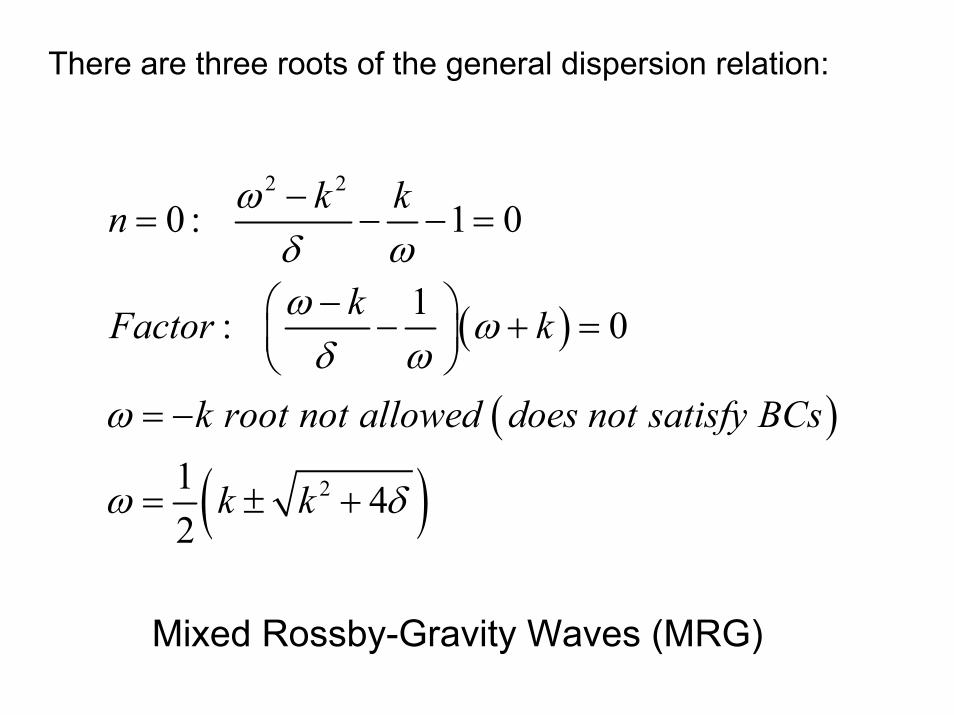
There are three roots of the general dispersion relation:
( )
( )
( )
2 2
2
0 : 1 0
1: 0
1 42
k kn
kFactor k
k root not allowed does not satisfy BCs
k k
ωδ ωω ωδ ω
ω
ω δ
−= − − =
−⎛ ⎞− + =⎜ ⎟⎝ ⎠
= −
= ± +
Mixed Rossby-Gravity Waves (MRG)
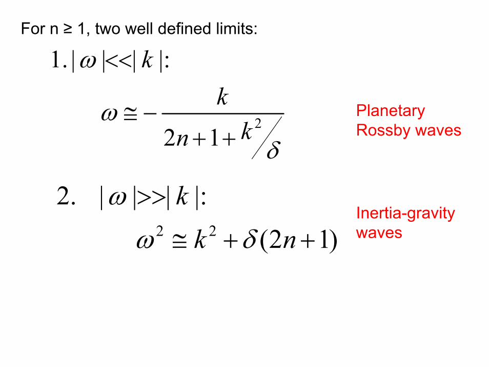
For n ≥ 1, two well defined limits:
2
1. | | | |:
2 1
kkkn
ω
ωδ
<<
≅ −+ +
Planetary Rossby waves
2 2
2. | | | |:(2 1)
kk n
ω
ω δ
>>
≅ + +Inertia-gravity waves
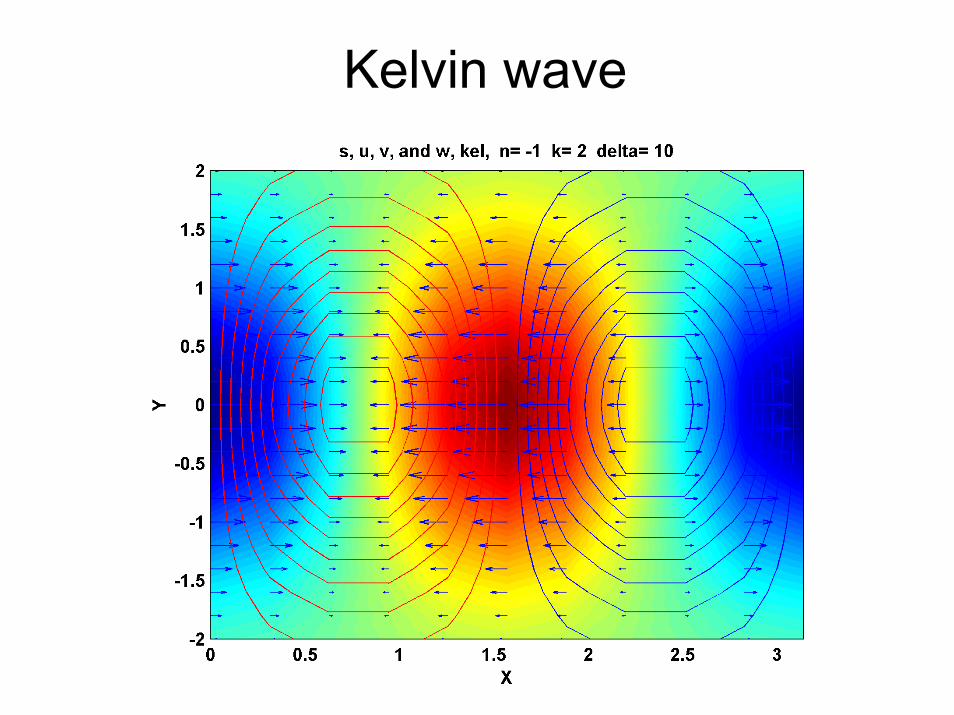
Kelvin wave
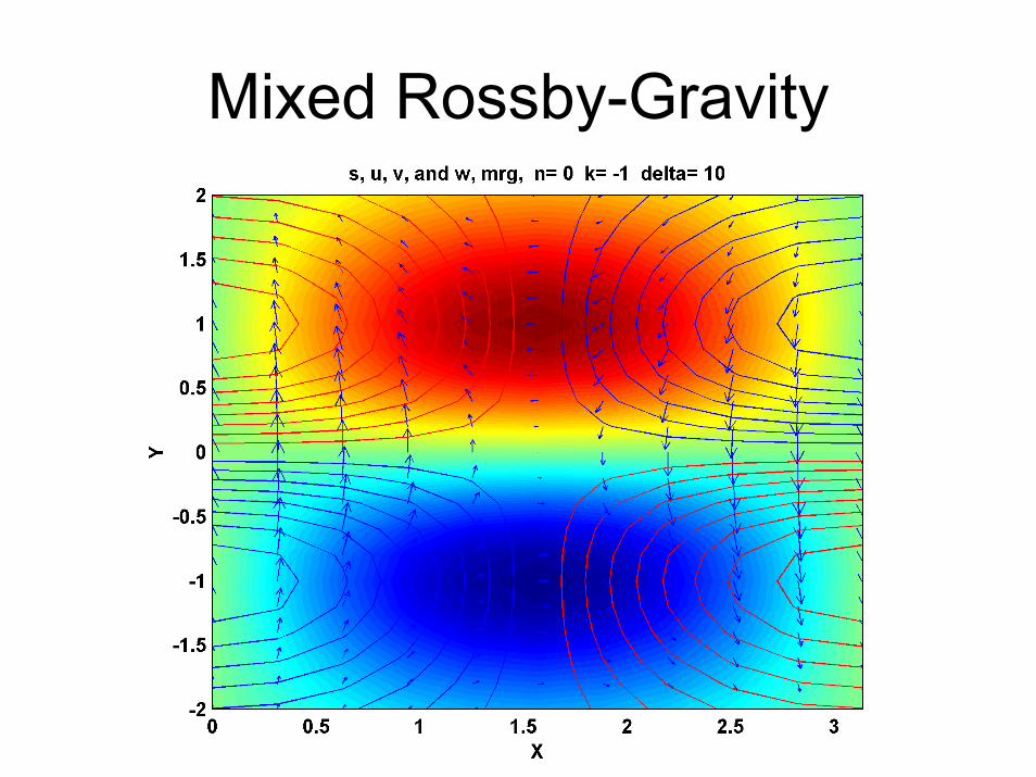
Mixed Rossby-Gravity
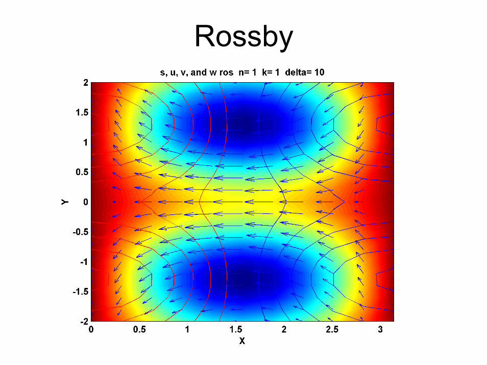
Rossby
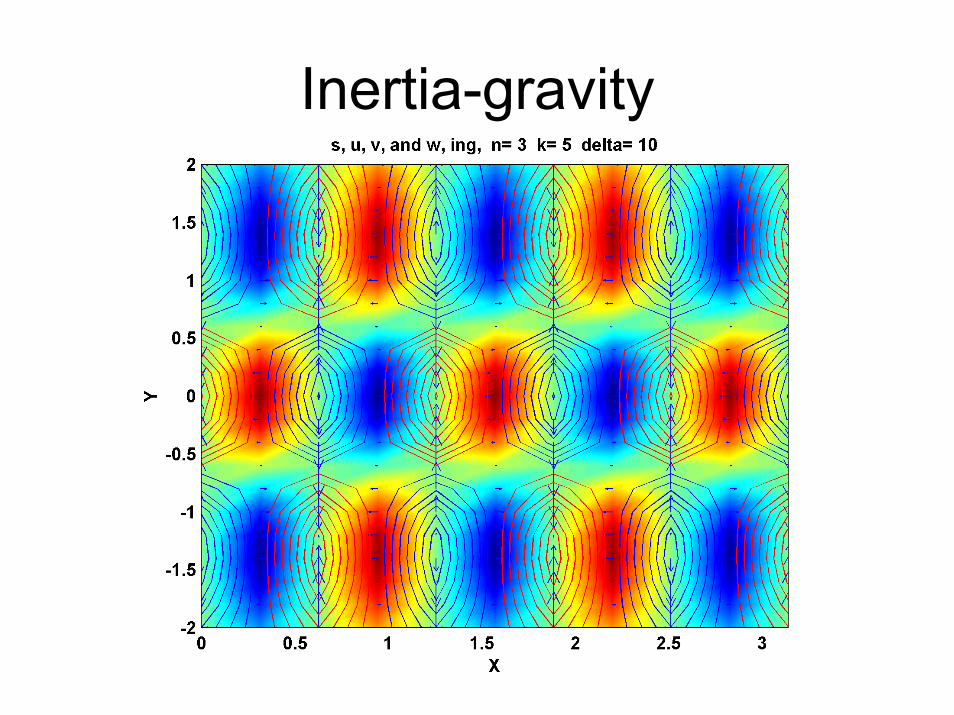
Inertia-gravity

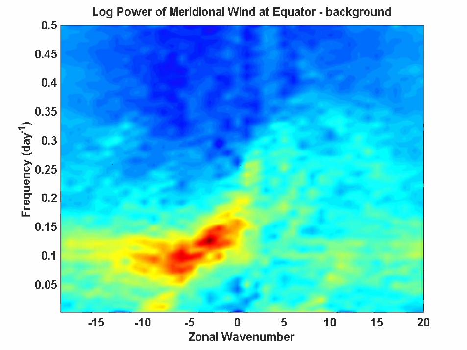
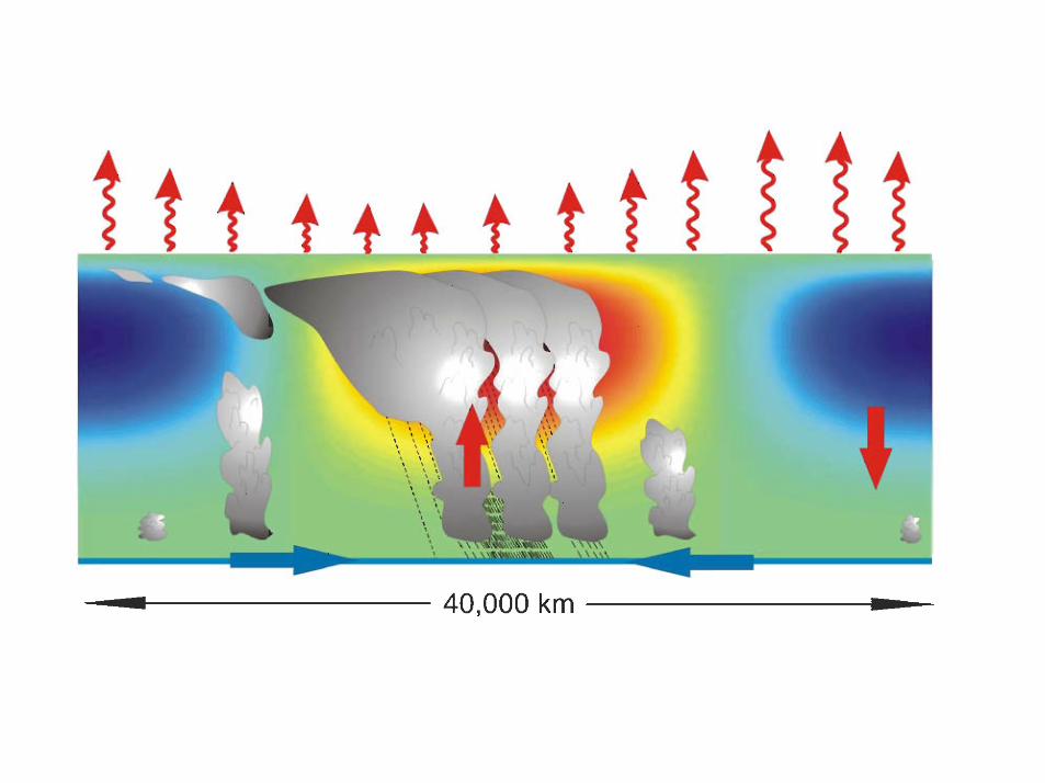
Intraseasonal Variability
• Stochastic excitation of the equatorial waveguide
• WISHE• Moisture-convection feedback• Cloud-radiation feedback• Ocean interaction
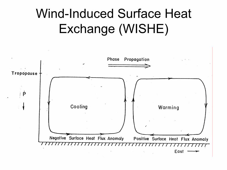
Wind-Induced Surface Heat Exchange (WISHE)

Add back WISHE term to linear undamped equations:
u s yvt x
∂ ∂= +
∂ ∂
v s yut y
δ⎛ ⎞∂ ∂
= −⎜ ⎟∂ ∂⎝ ⎠s u v ut x y
α∂ ∂ ∂= + +
∂ ∂ ∂

First look for Kelvin-like modes with v=0:
2 2
2 2
02 2
:ikx i t
u st xs u ut xu u ut x x
Let u u e
k i k
ω
α
α
ω α
−
∂ ∂=
∂ ∂∂ ∂
= +∂ ∂
∂ ∂ ∂→ = +
∂ ∂ ∂=
= −
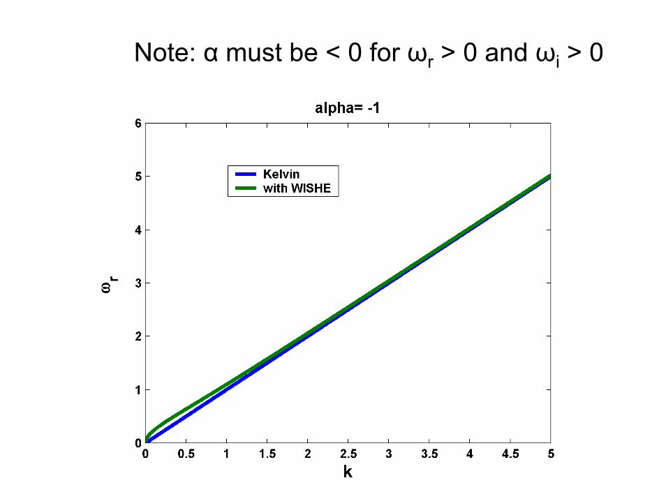
Note: α must be < 0 for ωr > 0 and ωi > 0

As k → ∞ ωi → -α/2
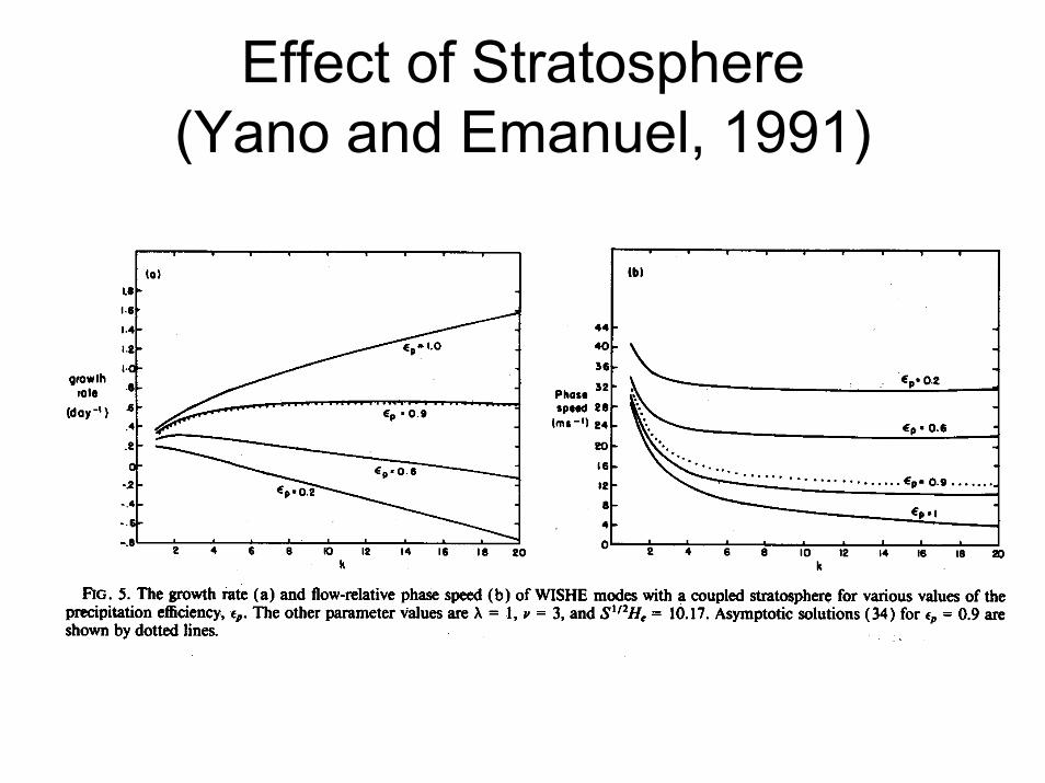
Effect of Stratosphere(Yano and Emanuel, 1991)

Effect of finite convective response time:
11
1
p
peq
p
eq
c
s u v Mt x y
u vM ux y
M MMt
ε
εα
ε
τ
⎛ ⎞∂ ∂ ∂= + +⎜ ⎟∂ − ∂ ∂⎝ ⎠
− ⎛ ⎞∂ ∂= + +⎜ ⎟− ∂ ∂⎝ ⎠
−∂=
∂


Go back to dimensional, quasi-linear QE equations on β plane”
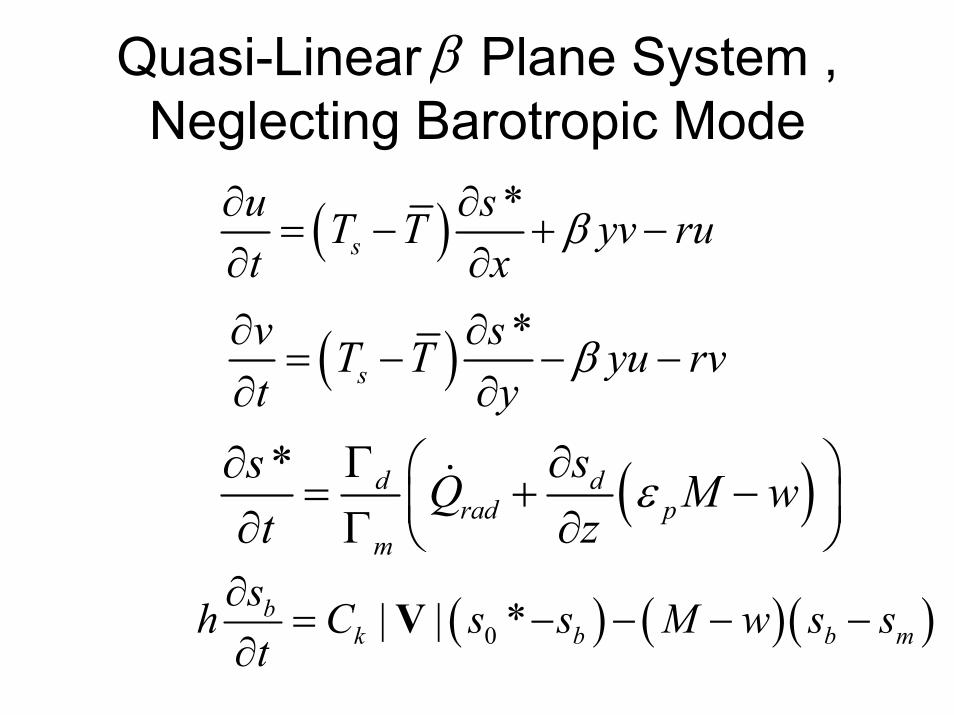
Quasi-Linear Plane System , Neglecting Barotropic Mode
β
( ) *s
u sT T yv rut x
β∂ ∂= − + −
∂ ∂
( ) *s
v sT T yu rvt y
β∂ ∂= − − −
∂ ∂
( )* d drad p
m
ss Q M wt z
εΓ ∂∂ ⎛ ⎞= + −⎜ ⎟∂ Γ ∂⎝ ⎠&
( ) ( )( )0| | *bk b b m
sh C s s M w s st
∂= − − − −
∂V
0u v wx y H∂ ∂
+ + =∂ ∂
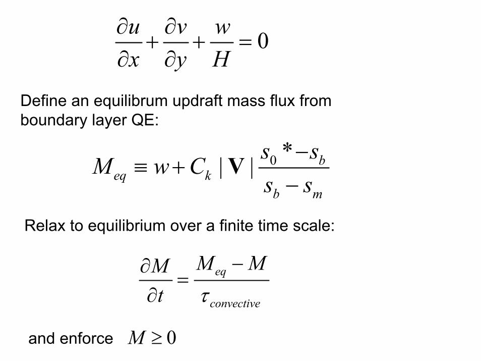
Define an equilibrum updraft mass flux from boundary layer QE:
0 *| | beq k
b m
s sM w Cs s
−≡ +
−V
Relax to equilibrium over a finite time scale:
eq
convective
M MMt τ
−∂=
∂
0M ≥and enforce

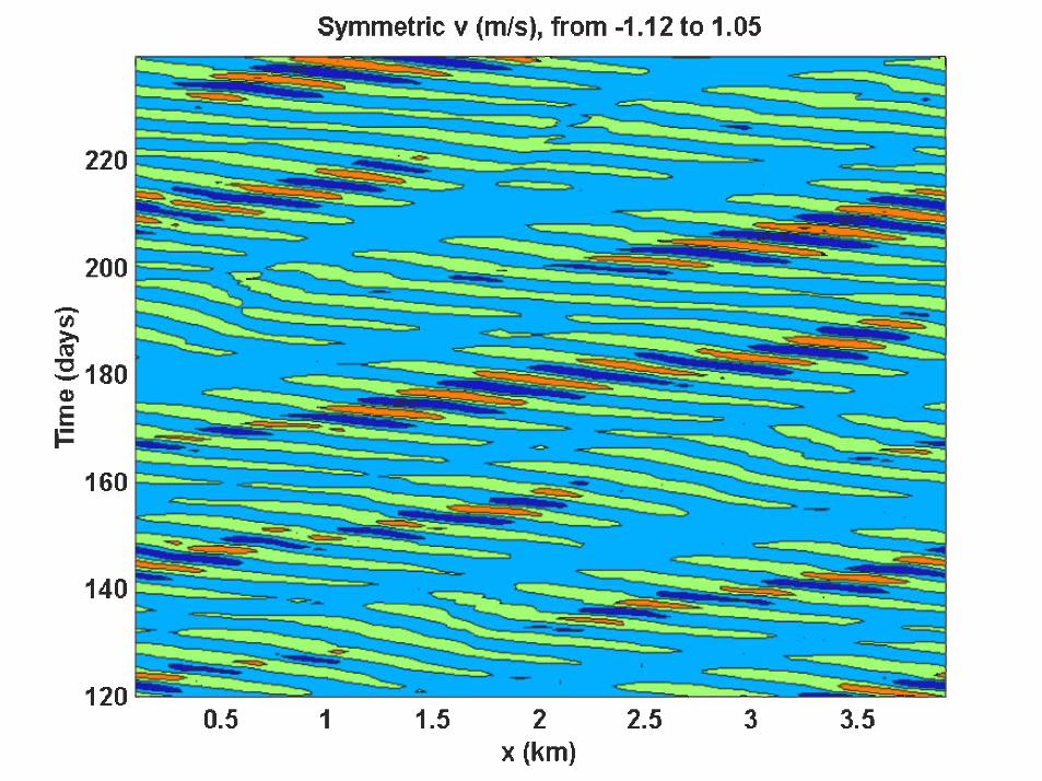
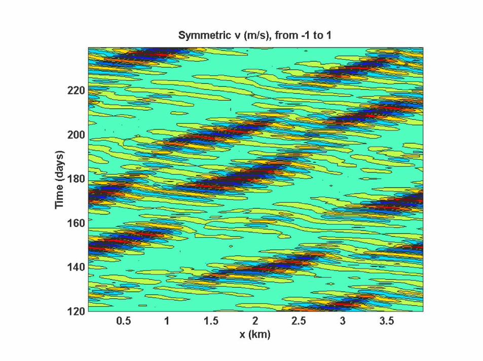
Numerical solution of β plane quasi-linear equations
• Nonlinearity retained only in surface fluxes• Zonally symmetric SST specified; also
symmetric about equator• Background easterly wind of 2 ms-1
imposed• Convection relaxed to equilibrium over
time scale of 3 hours


Cloud-Radiative Feedback• Set OLR proportional to difference in θe
between boundary layer and mid troposphere (Sandrine Bony)

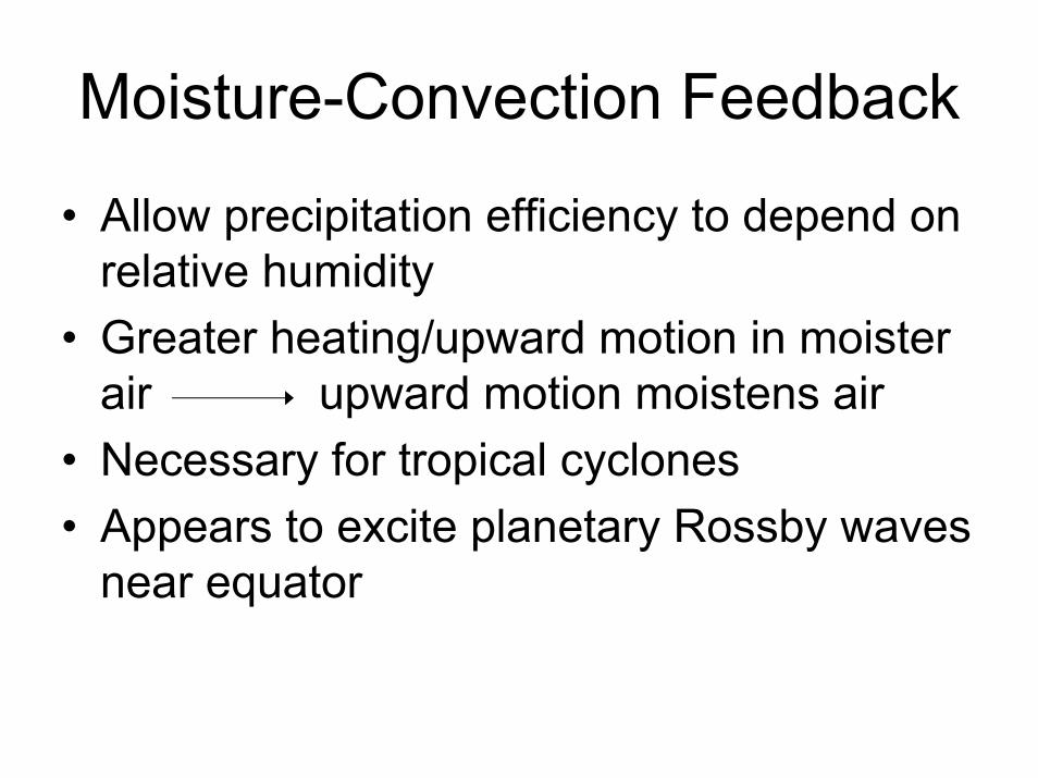
Moisture-Convection Feedback
• Allow precipitation efficiency to depend on relative humidity
• Greater heating/upward motion in moister air upward motion moistens air
• Necessary for tropical cyclones• Appears to excite planetary Rossby waves
near equator

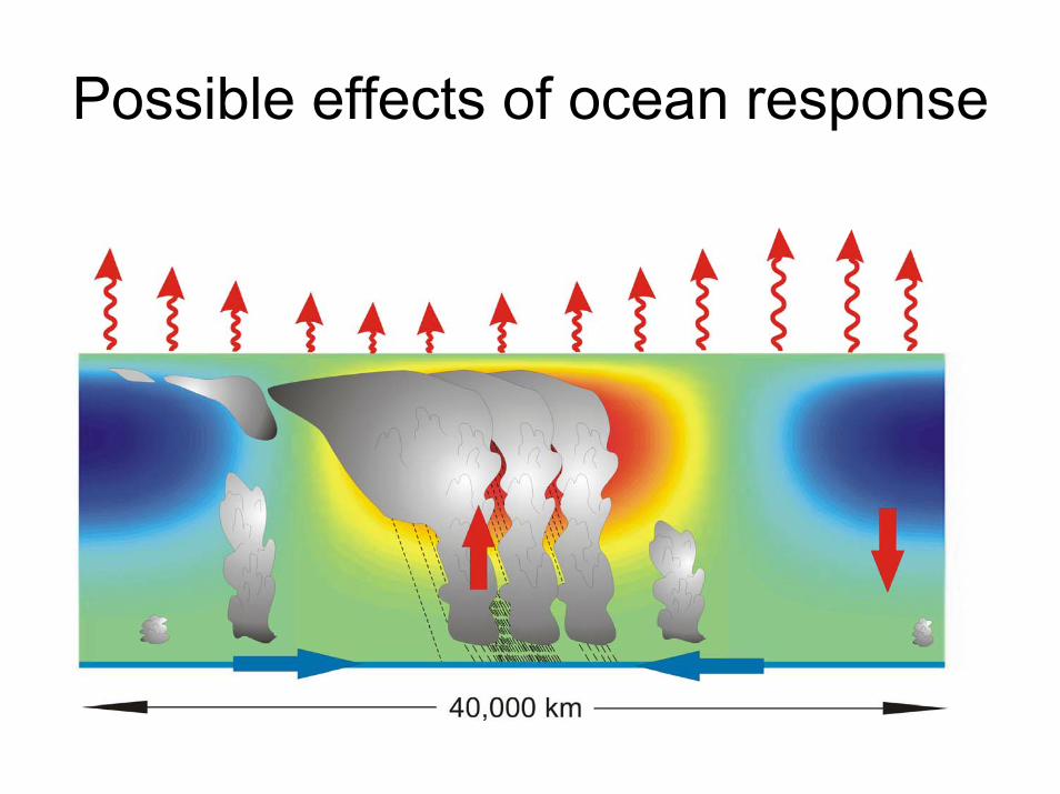
Possible effects of ocean response