1

Molecular Dynamics I: Principles Basics of the molecular-dynamics (MD) method1-3 are described, along with corresponding data structures in program, md.c. Newton’s Second Law of Motion TRAJECTORY, COORDINATE, AND ACCELERATION • Physical system = a set of atomic coordinates:

!

{r r i = (xi ,yi ,zi ) | xi ,yi ,zi "#,i = 0,...,N $1} ,

where ! is the set of real numbers (in the program, represented by a double precision variable) and we use a vector notation,

r r i.

(Data strcutures in md.c) int nAtom: N, the number of atoms. NMAX: Maximum number of atoms that can be handled by the program. double r[NMAX][3]: r[i][0], r[i][1], and r[i][2] are the x, y, and z coordinates of the i-th atom, where i = 0, .., N-1.

x

y

z

1 2

N

• Trajectory: A mapping from time to a point in the 3-dimensional space,

!

t "#ar r i (t)" #

3 . In fact, a trajectory of an N-atom system is regarded as a curve in 3N-dimensional space. A point on the curve is then specified by a 3N-element vector,

r r

N= (x

0, y0,z0, x1, y1,z1,..., xN!1, yN !1,zN !1 ) .

ri(t=0)

vi(t=0)

ri(t=t1)

vi(t=t1)

• Velocity: Short-time limit of an average speed (how fast and in which direction the particle is moving),

!

r v

i(t) =

r ˙ r i(t) =

dr r

dt" lim

#$0

r r i(t + #) %

r r i(t)

#.

double rv[NMAX][3]: rv[i][0], rv[i][1], and rv[i][2] are the x, y, and z components of the velocity vector,

r v

i, of the i-th atom.

• Acceleration: Rate at which a velocity changes (whether the particle is accelerating or decelerating),

!

r a i (t) =

r ˙ ̇ r i (t) =d

2r r

dt2

=dr v i

dt" lim#$0

r v i (t + #) %

r v i (t)

#.

2

double ra[NMAX][3]: ra[i][0], ra[i][1], and ra[i][2] are the x, y, and z components of the acceleration vector,

r a

i, of the i-th atom.

vi(t)

vi(t+!)

vi(t)

vi(t+!)

ai(t)!

The acceleration of a particle can be estimated from three consecutive positions on its trajectory separated by small time increments:

!

r a

i(t) = lim

"#0

r v

i(t + " /2) $

r v

i(t $" /2)

"

= lim"#0

r r i(t + ") $

r r i(t)

"$

r r i(t) $

r r i(t $")

"

"

= lim"#0

r r i(t + ") $ 2

r r i(t) +

r r i(t $")

"2

NEWTON’S EQUATION Newton’s equation states that the acceleration of a particle is proportional to the force acting on the particle,

m

r ˙ ̇ r i( t) =

r F

i(t) ,

where m is the mass of the particle. For a heavier particle, the same force causes less acceleration (or deceleration).

• Initial value problem: Given initial particle positions and velocities,

!

r r i (0),

r v i (0)( ) i = 0,...,N "1{ } ,

obtain those at later times,

!

r r i ( t),

r v i ( t)( ) i = 0,...,N "1;t # 0{ } . Note that both positions and velocities

must be specified in order to predict future trajectories.

Potential Energy We consider forces which are derived from a potential energy, V(

r r

N

) , which is a function of all atomic positions.

!

r F k = "

#

#r r k

Vr r

N( ) = "#V

#xk

,#V

#yk

,#V

#zk

$

% &

'

( ) .

Here partial derivative is defined as

!

"V

"xk= limh#0

V (x0,y0,z0,...,xk + h,yk,zk ,...xN$1,yN$1,zN$1) $V (x0,y0,z0,...,xk ,yk,zk ,...xN$1,yN$1,zN$1)

h,

i.e., what is the rate of change in V when we slightly change one coordinate of an atom while keeping all the other coordinates fixed. LENNARD-JONES POTENTIAL To model certain materials such as neon and argon liquids, the Lennard-Jones potential is often used by scientists:

3

!

Vr r

N( ) = u(rij )i< j

" =i= 0

N#2

" u(|r r ij |)

j= i+1

N#1

"

where

r r ij =

r r i !

r r j is the relative position vector between atoms i and j, and

!

u(r) = 4"#

r

$

% &

'

( ) 12

*#

r

$

% &

'

( ) 6+

, - -

.

/ 0 0 .

• Physical meaning of the potential: An atom consists of a nucleus and electrons surrounding it. Two atoms interact with each other in the following ways.

> Short-range repulsion (the first term): the Pauli exclusion principle states that electrons cannot occupy the same position, resulting in repulsion between the atoms. Note that for r → 0, this term is dominant.

> Long-range attraction (the second term): Electrons around nuclei polarize (change distribution),

creating electrostatic attraction between atoms. Note that for r → ∞, this term becomes dominant.

• For Argon atoms, > m = 6.6 × 10-23 gram > ε = 1.66 × 10-14 erg (erg = gram•cm2/(second2) is a unit of energy) > σ = 3.4 × 10-8 cm

* Don’t program with these numbers (in the CGS unit); it will cause floating-point under- or over-flows. NORMALIZATION • We introduce normalized coordinates,

r ! r

i, potential energy, V', and time, t', that are dimensionless

and are defined as follows.

!

r r i=

r " r

i# = 3.4 $10%8[cm]$

r " r

i

V = " V & =1.66 $10%14[erg]$ " V

t =# m /& " t = 2.2 $10%12[sec]$ " t

'

( )

* )

With these substitutions, Newton’s equation becomes

!

m"

m# 2#

d2r $ r

i

d $ t 2

= %"

#

& $ V

&r $ r

i

.

* In the derivation above, note that

!

md2r r i

dt2

= m lim"#0

r r i(t + ") $ 2

r r i(t) +

r r i(t $")

"2

= m lim"#0

%r & r

i(t + ") $ 2

r & r

i(t) +

r & r

i(t $")[ ]

% m /'[ ]2

& " ( )2

4

In summary, the normalized Newton’s equation for atoms interacting with the Lennard-Jones potential is given below. (From now on, we always use normalized variables, and omit primes.)

d2 r r i

dt2= !

"V

"r r i

=r a i

V(r r

N) = u(rij )

i < j

#

u(r) = 41

r12 !

1

r6

$

% &

'

( )

The figure in the right shows the normalized Lennard-Jones potential, u(r), as a function of interatomic distance, r. The distance, r0, at which the potential takes its minimum value, u(r0), is obtained as follows.

du

dr r =r0

= 0 ! r0 = 21/6 "1.12

u(r0 ) = 41

212/ 6#1

26 / 6

$

% &

'

( ) = #1

-1

-0.5

0

0 0.5 1 1.5 2 2.5 3

u(r

)/!

r/"

21/6

~ 1.12

Figure: Lennard-Jones potential.

ANALYTIC FORMULA FOR FORCES

!

r a k = "

#

#r r k

u(rij )i< j

$

= "#rij

#r r ki< j

$du

drij

Let’s evaluate the two factors in the above expression:

1.

!

"rij

"r r k

="

"xk

,"

"yk

,"

"zk

#

$ %

&

' ( xi ) x j( )

2

+ yi ) y j( )2

+ zi ) z j( )2

=2(xi ) x j ),2(yi ) y j ),2(zi ) z j )( )

2 xi ) x j( )2

+ yi ) y j( )2

+ zi ) z j( )2*ik )* jk( )

=

r r ij

rij

*ik )* jk( )

Qd

dxf (x)[ ]

1/ 2=1

2f (x)[ ]

)1/ 2 df

dx

#

$ %

&

' (

2.

!

du

dr= 4 "

12

r13

+6

r7

#

$ %

&

' ( = "

48

r

1

r12"1

2r6

#

$ %

&

' (

Qd

drr"n

= "nr"n"1#

$ %

&

' (

In the first result,

5

!ik

=1 (i = k)

0 (i " k)

# $ %

is called Kronecker’s delta expression. Substituting these two results back into the expression for

r a

k, we obtain

r a k =

r r ij !

1

r

du

dr

"

# $

%

& '

r= riji< j

( ) ik ! ) jk( )

where

!1

r

du

dr=48

r2

1

r12!1

2r6

"

# $

%

& '

Summary of Molecular-Dynamics Equation System

Given initial atomic positions and velocities,

!

r r i (0),

r v i (0)( ) i = 0,...,N "1{ } , obtain those at later times,

!

r r i ( t),

r v i ( t)( ) i = 0,...,N "1;t # 0{ } , by integrating the following differential equation:

!

r ˙ ̇ r k (t) =r a k (t) = "

#

#r r k

u rij( ) =i< j

$r r ij (t) "

1

r

du

dr

%

& '

(

) *

r= rij ( t )i< j

$ +ik "+ jk( )

where

!

"1

r

du

dr=48

r2

1

r12"1

2r6

#

$ %

&

' (

The sum over i and j to evaluate the acceleration is implemented in a program as follows: for i = 0 to N-1,

r a i = 0

for i = 0 to N-2 for j = i+1 to N-1

compute

!

r " =

r r ij #

1

r

du

dr

$

% &

'

( )

r=r r ij

r a i + =

r !

r a j ! =

r "

Discretization We need to discretize the trajectories in order to solve the problem on a computer: Instead of considering

r r i(t),

r v

i(t)( ) for t ! 0

for continuous time, we consider a sequence of states

r r i(0),

r v

i(0)( ) a

r r i(!),

r v

i(!)( )a

r r i(2!),

r v

i(2!)( ) aL

ri(0)

ri(2!)ri(!)

The question is: How to predict the next state,

r r i(t + !),

r v

i(t + !)( ) , from the current state,

r r i(t),

r v

i(t)( ) ?

6

double DeltaT: Δ in md.c.

VERLET DISCRETIZATION Let’s apply the Taylor expansion

!

f (x0 + h) =hn

n!n=0

"

#dnf

dxn

x=x0

= f (x0) + hdf

dx x=x0

+h2

2

d2f

dx2

x=x0

+h3

3!

d3f

dx3

x=x0

+L,

which predicts a function value at a distant point, x0+h, from derivatives at x0, to an atomic coordinate.

!

r r i(t + ") =

r r i(t) +

r v

i(t)" +

1

2

r a

i(t)"

2+

1

6

r ˙ ̇ ̇ r i(t)"

3+ O("

4)

+r r i(t #") =

r r i(t) #

r v

i(t)" +

1

2

r a

i(t)"

2#

1

6

r ˙ ̇ ̇ r i(t)"

3+ O("

4)

!

r r i(t + ") +

r r i(t #") = 2

r r i(t) +

r a

i(t)"

2+ O("

4)

!

"r r i(t + #) = 2

r r i(t) $

r r i(t $#) +

r a

i(t)#

2+ O(#

4)

To obtain velocities,

!

r r i(t + ") =

r r i(t) +

r v

i(t)" +

1

2

r a

i(t)"

2+

1

6

r ˙ ̇ ̇ r i(t)"

3+ O("

4)

#r r i(t #") =

r r i(t) #

r v

i(t)" +

1

2

r a

i(t)"

2#

1

6

r ˙ ̇ ̇ r i(t)"

3+ O("

4)

!

r r

i(t + ") #

r r

i(t #") = 2

r v

i(t)" + O("

3)

!

"r v i (t) =

r r i (t + #) $

r r i (t $#)

2#+ O(#

2)

The above two results constitute the Verlet discretization scheme.

(Verlet discretization scheme)

!

r r i (t + ") = 2

r r i (t) #

r r i (t #") +

r a i (t)"

2+ O("4 ) (1)

r v i (t) =

r r i (t + ") #

r r i (t #")

2"+ O("2) (2)

$

% &

' &

The Verlet algorithm for MD integration is a straight-forward application of these two equations.

(Verlet algorithm) Given

r r i(t ! ") and

r r i(t) ,

1. Compute

r a

i(t) as a function of

{r r i(t)} ,

2.

r r i(t + !)" 2

r r i(t) #

r r i(t # !) +

r a

i(t)!

2 , 3.

!

r v i (t)"

r r i (t + #) $

r r i (t $#)[ ] 2#( ) ,

A problem of this discretization scheme is that the velocity at time t cannot be calculated until the coordinate at time t+Δ is calculated. In the slight variation, called the velocity-Verlet scheme, of the above discretization scheme, we are given

r r i(t),

r v

i(t)( ) and predict

r r i(t + !),

r v

i(t + !)( ) .

7

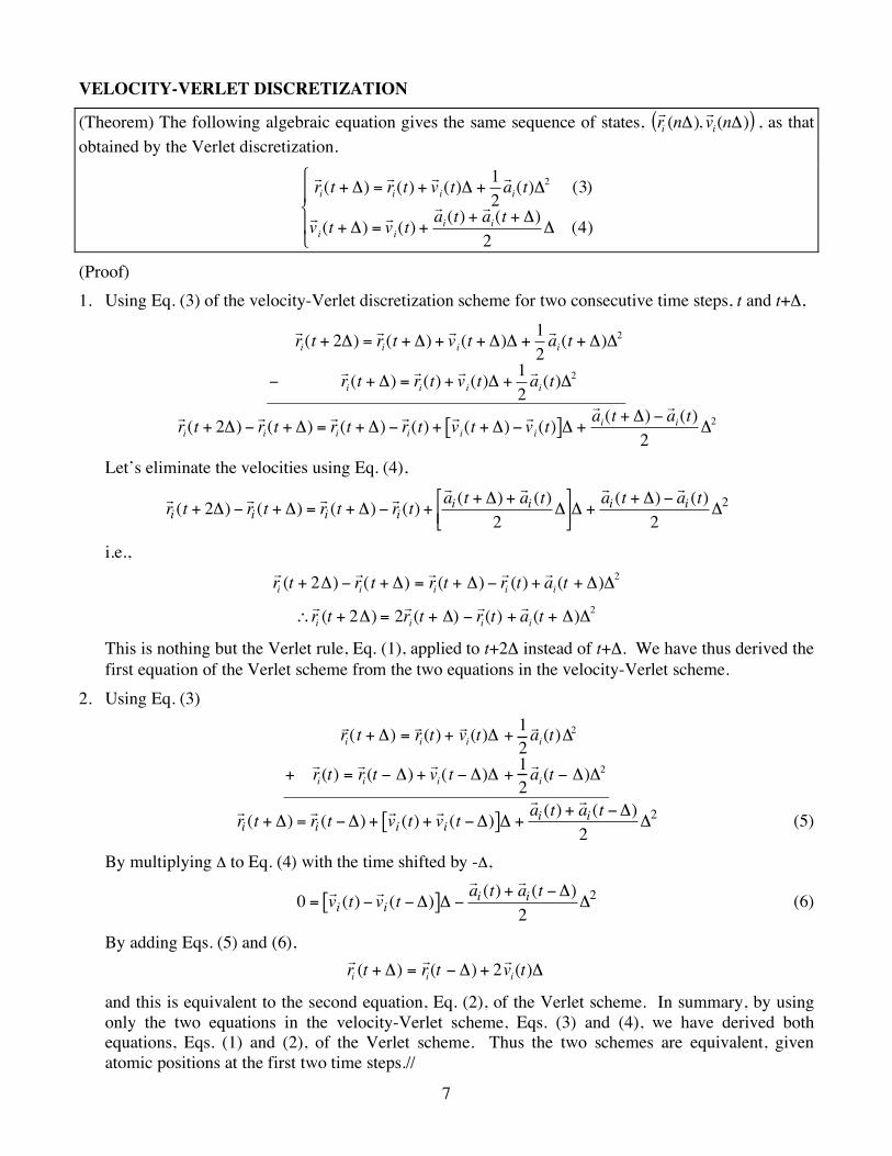
VELOCITY-VERLET DISCRETIZATION

(Theorem) The following algebraic equation gives the same sequence of states,

r r i(n!),

r v

i(n!)( ) , as that

obtained by the Verlet discretization.

!

r r i(t + ") =

r r i(t) +

r v

i(t)" +

1

2

r a

i(t)"2 (3)

r v

i(t + ") =

r v

i(t) +

r a

i(t) +

r a

i(t + ")

2" (4)

#

$ %

& %

(Proof) 1. Using Eq. (3) of the velocity-Verlet discretization scheme for two consecutive time steps, t and t+Δ,

!

r r i(t + 2") =

r r i(t + ") +

r v

i(t + ")" +

1

2

r a

i(t + ")"

2

#r r i(t + ") =

r r i(t) +

r v

i(t)" +

1

2

r a

i(t)"

2

!

r r i(t + 2") #

r r i(t + ") =

r r i(t + ") #

r r i(t) +

r v

i(t + ") #

r v

i(t)[ ]" +

r a

i(t + ") #

r a

i(t)

2"2

Let’s eliminate the velocities using Eq. (4),

!

r r i (t + 2") #

r r i (t + ") =

r r i (t + ") #

r r i (t) +

r a i (t + ") +

r a i (t)

2"

$

% & '

( ) " +

r a i (t + ") #

r a i (t)

2"2

i.e.,

r r i(t + 2!) "

r r i( t + !) =

r r i(t + !) "

r r i(t) +

r a

i(t + !)!

2

!

r r i(t + 2") = 2

r r

i(t + ") #

r r i(t) +

r a

i(t + ")"

2

This is nothing but the Verlet rule, Eq. (1), applied to t+2Δ instead of t+Δ. We have thus derived the first equation of the Verlet scheme from the two equations in the velocity-Verlet scheme.

2. Using Eq. (3)

r r i( t + !) =

r r i(t) +

r v

i(t)! +

1

2

r a

i(t)!2

+r r i(t) =

r r i(t " !) +

r v

i( t " !)! +

1

2

r a

i(t " !)!2

!

r r i (t + ") =

r r i (t #") +

r v i (t) +

r v i (t #")[ ]" +

r a i (t) +

r a i (t #")

2"2 (5)

By multiplying Δ to Eq. (4) with the time shifted by -Δ,

!

0 =r v i (t) "

r v i (t "#)[ ]# "

r a i (t) +

r a i (t "#)

2#2 (6)

By adding Eqs. (5) and (6),

r r i(t + !) =

r r i(t " !) + 2

r v

i(t)!

and this is equivalent to the second equation, Eq. (2), of the Verlet scheme. In summary, by using only the two equations in the velocity-Verlet scheme, Eqs. (3) and (4), we have derived both equations, Eqs. (1) and (2), of the Verlet scheme. Thus the two schemes are equivalent, given atomic positions at the first two time steps.//

8

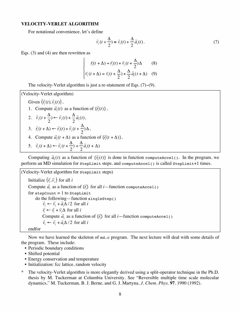
VELOCITY-VERLET ALGORITHM For notational convenience, let’s define

r v

i(t +

!

2) "

r v

i(t) +

!

2

r a

i(t) . (7)

Eqs. (3) and (4) are then rewritten as

r r i(t + !) =

r r

i(t) +

r v

i(t +

!

2)! (8)

r v

i(t + !) =

r v

i(t +

!

2) +

!

2

r a

i( t + !) (9)

"

# $ $

% $ $

The velocity-Verlet algorithm is just a re-statement of Eqs. (7)−(9).

(Velocity-Verlet algorithm)

Given

r r i(t),

r v

i(t)( ) ,

1. Compute

r a

i(t) as a function of

{r r i(t)} ,

2.

!

r v

i(t +

"

2)#

r v

i(t) +

"

2

r a

i(t),

3.

r r i(t + !)"

r r

i(t) +

r v

i(t +

!

2)! ,

4. Compute

r a

i(t + !) as a function of

{r r i(t + !)},

5.

r v

i(t + !)"

r v

i(t +

!

2) +

!

2

r a

i(t + !)

Computing

!

r a i (t) as a function of

!

{r r i (t)} is done in function computeAccel(). In the program, we

perform an MD simulation for StepLimit steps, and computeAccel() is called StepLimit+1 times.

(Velocity-Verlet algorithm for StepLimit steps)

Initialize

r r i,r v

i( ) for all i

Compute

r a

i as a function of

{r r i} for all i—function computeAccel()

for stepCount = 1 to StepLimit do the following—function singleStep()

r v

i!

r v

i+

r a

i" / 2 for all i

r r i!

r r i+

r v

i" for all i

Compute

r a

i as a function of

{r r i} for all i—function computeAccel()

r v

i!

r v

i+

r a

i" / 2 for all i

endfor

Now we have learned the skeleton of md.c program. The next lecture will deal with some details of the program. These include:

• Periodic boundary conditions • Shifted potential • Energy conservation and temperature • Initialization: fcc lattice, random velocity

* The velocity-Verlet algorithm is more elegantly derived using a split-operator technique in the Ph.D. thesis by M. Tuckerman at Columbia University. See “Reversible multiple time scale molecular dynamics,” M. Tuckerman, B. J. Berne, and G. J. Martyna, J. Chem. Phys. 97, 1990 (1992).

9

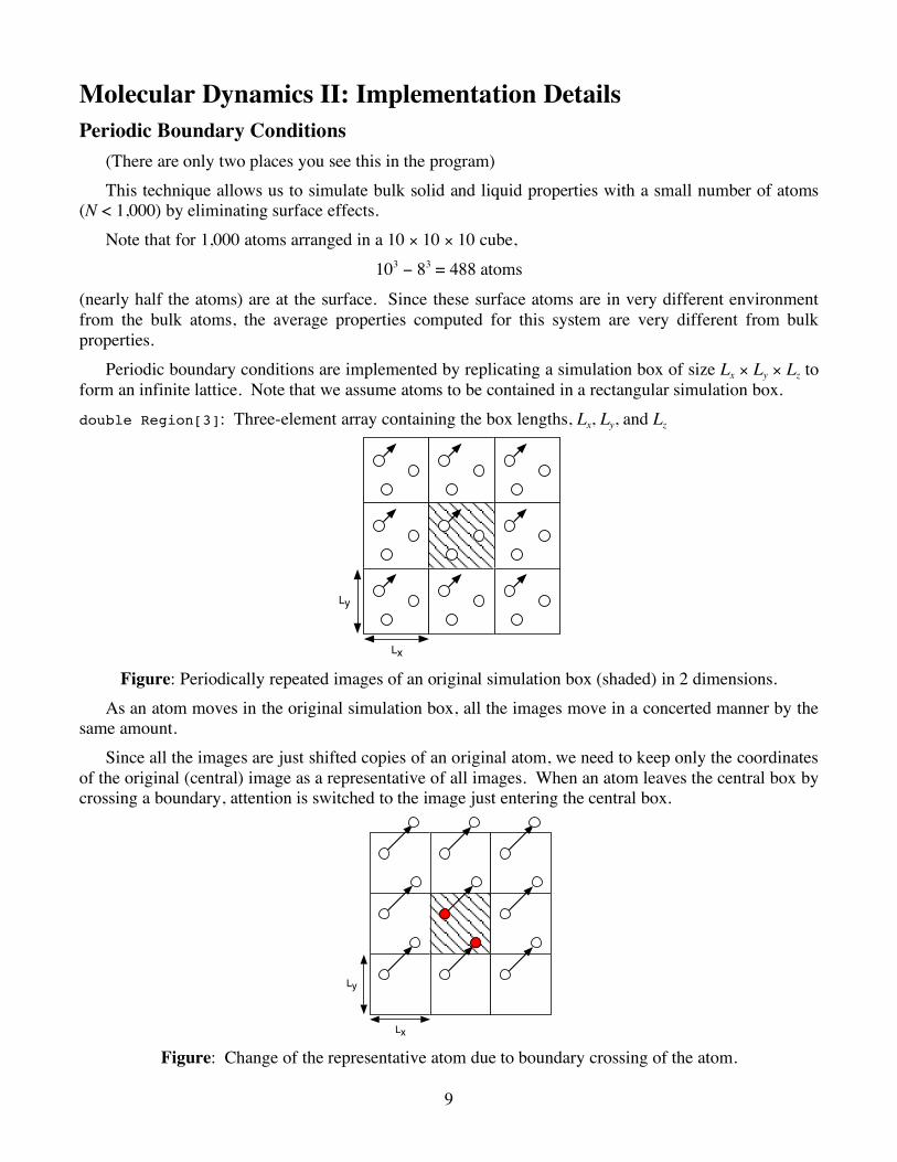
Molecular Dynamics II: Implementation Details Periodic Boundary Conditions (There are only two places you see this in the program) This technique allows us to simulate bulk solid and liquid properties with a small number of atoms (N < 1,000) by eliminating surface effects. Note that for 1,000 atoms arranged in a 10 × 10 × 10 cube,

103 − 83 = 488 atoms

(nearly half the atoms) are at the surface. Since these surface atoms are in very different environment from the bulk atoms, the average properties computed for this system are very different from bulk properties. Periodic boundary conditions are implemented by replicating a simulation box of size Lx × Ly × Lz to form an infinite lattice. Note that we assume atoms to be contained in a rectangular simulation box. double Region[3]: Three-element array containing the box lengths, Lx, Ly, and Lz

Lx

Ly

Figure: Periodically repeated images of an original simulation box (shaded) in 2 dimensions.

As an atom moves in the original simulation box, all the images move in a concerted manner by the same amount. Since all the images are just shifted copies of an original atom, we need to keep only the coordinates of the original (central) image as a representative of all images. When an atom leaves the central box by crossing a boundary, attention is switched to the image just entering the central box.

Lx

Ly

Figure: Change of the representative atom due to boundary crossing of the atom.

10

At every MD step, we enforce that an atomic coordinate satisfies 0 ≤ xi < Lx, 0 ≤ yi < Ly, 0 ≤ zi < Lz.

If

r r i(t) is in the central box and time increment Δ is small,

r r i(t + !) is at most in the neighbor image

(if this assumption becomes invalid, then exceptions may occur during program execution): -Lx ≤ xi(t+Δ) < 2Lx, etc. In this case, an atom can be “pulled back” to the central box by

!

xi " xi #SignRLx

2,xi

$

% &

'

( ) #SignR

Lx

2,xi # Lx

$

% &

'

( )

yi " yi #SignRLy

2,yi

$

% &

'

( ) #SignR

Ly

2,yi # Ly

$

% &

'

( )

zi " zi #SignRLz

2,zi

$

% &

'

( ) #SignR

Lz

2,zi # Lz

$

% &

'

( )

*

+

, , ,

-

, , ,

where

!

SignRLx

2,x

i

"

# $

%

& ' =

Lx

2xi> 0

(Lx

2xi) 0

*

+ ,

- ,

and this means

!

Lx

< xi

xi"Lx

2"Lx

2= x

i" L

x

0 < xi# L

xxi"Lx

2+Lx

2= x

i

xi# 0 x

i+Lx

2+Lx

2= x

i+ L

x

$

%

& &

'

& &

double RegionH[3]: An array (Lx/2, Ly/2, Lz/2)

Minimum Image Convention In principle, an atom interacts with all the images of another atom (and even with its own images except for itself). In practice, we make the simulation box larger enough so that u(r > Lx/2) etc. can be neglected. Then an atom interacts with only the nearest image of another atom.

Lx

Ly

i j

11

Or we can imagine a box of size Lx × Ly × Lz centered at atom i, and this atom interacts only with other atoms in this imaginary box. Therefore,

!

"Lx

2# xij <

Lx

2

"Ly

2# yij <

Ly

2

"Lz

2# zij <

Lz

2

$

%

& & &

'

& & &

during the computation of forces. In the program, this is achieved by

!

xij " xij #SignRLx

2,xij +

Lx

2

$

% &

'

( ) #SignR

Lx

2,xi #

Lx

2

$

% &

'

( )

yij " yij #SignRLy

2,yij +

Ly

2

$

% &

'

( ) #SignR

Lx

2,yij #

Lx

2

$

% &

'

( )

zij " zij #SignRLz

2,zij +

Lz

2

$

% &

'

( ) #SignR

Lz

2,zij #

Lz

2

$

% &

'

( )

*

+

, , ,

-

, , ,

Shifted Potential With the minimal image convention, interatomic interaction is cut-off at half the box length. If the box is not large enough, this truncation causes a significant discontinuity in the potential function and our derivation of forces breaks down (we cannot differentiate the potential).

u(r)

r

Lx/2

Potential energy jump

To remedy this, we introduce a cut-off length rc < Lx/2 etc. and modify the potential such that both u(r) and du/dr are continuous at rc.

!

" u (r) =u(r) # u(rc) # (r # rc)

du

drr=r

c

r < rc

0 r $ rc

%

& '

( '

For the Lennard-Jones potential, rc = 2.5σ is conventionally used. This causes some shift in the potential minimum but little shift in the minimum position.

12

-1

-0.5

0

0 0.5 1 1.5 2 2.5 3

u(R)

u'(R)u(R

)/!

R/"

Rc

21/6

~ 1.12

Figure: Truncated Lennard-Jones potential.

Energy In addition to the potential energy, V, introduced before, we introduce the kinetic energy, K, and the total energy, E, as a sum of both.

!

E = K + V

=m

2

r ˙ r i2

i=0

N"1

# + u(rij )i< j

#

where

!

r ˙ r i2

= ˙ x i2

+ ˙ y i2

+ ˙ z i2 .

ENERGY CONSERVATION We can prove that the total energy, E, does not change in time, if Newton’s equation is exactly integrated. In order to prove the energy conservation, let us consider

!

˙ E = ˙ K + ˙ V

=m

2

d

dt˙ x i

2 + ˙ y i2 + ˙ z i

2( )i=0

N"1

# +dxi

dt

$V

$xi

+dyi

dt

$V

$yi

+dzi

dt

$V

$zi

%

& '

(

) *

i=0

N"1

#

=m

22 ˙ x i ˙ ̇ x i + ˙ y i ˙ ̇ y i + ˙ z i˙ ̇ z i( )

i=0

N"1

# + ˙ x i$V

$xi

+ ˙ y i$V

$yi

+ ˙ z i$V

$zi

%

& '

(

) *

i=0

N"1

#

= mr ˙ r i •

r ˙ ̇ r ii=0

N"1

# +r ˙ r i •

$V

$r r ii=0

N"1

#

=r ˙ r i

i=0

N"1

# • mr ˙ ̇ r i "

r F i( )

From Newton’s equation, the last expression is zero. In the derivation, vector inner product is defined as

13

r a •

r b = (ax ,ay,az )• (bx,by,bz ) = axbx + ayby + azbz

and note that d

dtfg( ) = ˙ f g + f ˙ g .

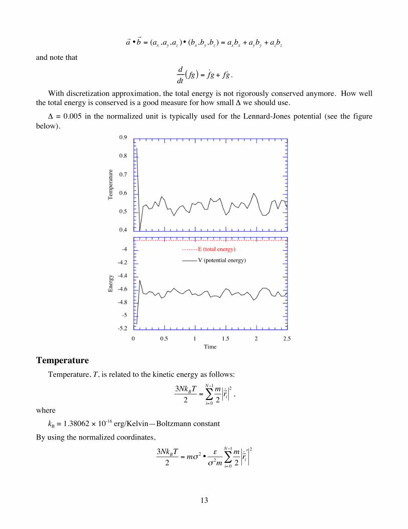
With discretization approximation, the total energy is not rigorously conserved anymore. How well the total energy is conserved is a good measure for how small Δ we should use.

Δ = 0.005 in the normalized unit is typically used for the Lennard-Jones potential (see the figure below).

Temperature Temperature, T, is related to the kinetic energy as follows:

!

3NkBT

2=

m

2

r ˙ r i

2

i= 0

N"1

# ,

where kB = 1.38062 × 10-16 erg/Kelvin—Boltzmann constant

By using the normalized coordinates,

!

3NkBT

2= m" 2

•#

" 2m

m

2

r ˙ r i

$2

i= 0

N%1

&

14

!

"T

# /kB

=1

3N

r ˙ r i

$2

i= 0

N%1

&

where ε/kB = 120 Kelvin

is the Lennard-Jones temperature unit. So the average temperature 0.5 means 60 K << 273 K = 0°C.

Initialization The program starts to initialize the coordinates and velocities of all atoms. FACE CENTERED CUBIC (FCC) LATTICE Atoms are initially arranged to form a regular lattice. Namely they occupy all the corners and face centers of a cube called a unit cell.

cx

cz

cy

double gap[3]: (cx, cy, cz), the edge lengths of the unit cell Since our unit cell is cubic, cx = cy = cz = c. Each unit cell contains

1

8! 8(corners) +

1

2! 6(faces) = 4atoms ,

and the number density of atoms is given by ! = 4 / c3 , or

c = 4 / !( )1 / 3 .

The four coordinates are given (in unit of c) as: (0, 0, 0), (0, 1/2, 1/2), (1/2, 0, 1/2), (1/2, 1/2, 0). These four coordinates are stored in double origAtom[4][3]

The simulated system is constructed by repeating the unit cells. int InitUcell[3]: Stores the number of unit cells in the x, y, and z directions The total number of atoms is therefore given by

N = 4 × InitUcell[0] × InitUcell[1] × InitUcell[2]

RANDOM VELOCITY We generate random velocities of magnitude

!

v0

2

3= T

init" v

0= 3T

init

double InitTemp: Initial temperature

15

For each atom, the velocity vector is then given by

r v

i= v

0!0,!1,!2

( ) = v0

r

!

where r

! is a rondomly oriented vector of unit length.

RANDOM POINT IN A UNIT CIRCLE The question is how to randomly generate a point on a unit sphere. We first start from a simpler problem, random point in a unit circle.

x

y

1-1

-1

1

(Algorithm) Let rand() be a uniform random-number generator in the range [0, 1] 1. ζi = 2*rand() - 1 (i = 0, 1) so that -1 ≤ ζi < 1 2. s

2

= !0

2

+!1

2 3. if s2 < 1, accept

v

! = (!0,!1)

4. else reject and go to 1 (Probability distribution)

x

y

1-1

-1

1

!0

!1

d!0

d!1

Probability to find a point in the shaded area = (# of points in the shaded area)/(total # of generated points) = P(ζ0, ζ 1)d ζ 0d ζ 1

= (d ζ 0d ζ 1 ~ shaded area)/(π•12 ~ area of unit circle), if there is no bias

!P("0,"1) = 1/#

(Polar coordinate system) (! 0 ,!1) = scos" , ssin"( ) 0 # s <1;0 # " < 2$

16

x

y

1-1

-1

1

!s ds

d!

Again the probability density is given by the ratio of the shaded area divided by the total circular area.

P(s,! )dsd! =ds • sd!

" •12

(if uniform)

!P(s," ) =s

# (1)

RANDOM POINT ON A UNIT SPHERE The above distribution is closely related to the uniform distribution on a unit sphere. (Spherical coordinate)

y

z

x

d!

!

"

sin(!)d"

(!0,!1,!2 ) = (sin" cos#, sin" sin#,cos" ) 0 $" < % ,0 $ # < 2%

(Probability distribution)

P(!,")d!d" =d! • sin!d"

4# •12

!P(",#) =sin"

4$ (2)

If we identify s ! sin "2

, Eqs. (1) and (2) are equivalent.

Q0 ! " < # $ 0 !"

2<#

2$ 0 ! s % sin

"

2<1

sdsd!

"=

sin#

2

ds

d#d#d!

"=

sin#

2

1

2cos

#

2

$

% &

'

( ) d#d!

"=

2sin#

2cos

#

2d#d!

4"=sin#d#d!

4"//

17

Note that

!

"0

= sin# cos$ = 2sin#

2cos

#

2cos$ = 2s 1% s2

&0

s= 2 1% s2&

0

"1

= sin# sin$ = 2sin#

2cos

#

2sin$ = 2s 1% s2

&1

s= 2 1% s2&

1

"2

= cos# =1% 2sin2#

2=1% 2s2

'

(

) )

*

) )

(Algorithm—Generating random points on a unit sphere) Let rand() be a uniform random-number generator in the range [0, 1] 1. ζi = 2*rand() - 1 (i = 0, 1) so that -1 ≤ ζi < 1 2. s

2

= !0

2

+!1

2 3. if s2 < 1, accept

!

("0,"1,"2) = (2 1# s

2$0,2 1# s

2$1,1# 2s

2)

4. else reject and go to 1

LINEAR CONGRUENTIAL RANDOM NUMBER GENERATOR Sequence of seemingly random integers between 1 and m-1 is obtained by starting from some nonzero I1 and

I j+1 = aIj (mod m)

We choose m = 231-1 = 2147483647 a = 16807 Uniform random number in the range [0, 1] is obtained as

r j= I j /m .

18

Molecular Dynamics III: O(N) Linked-List Cell Algorithm This chapter explains the linked-list cell MD algorithm, the computational time of which scales as O(N) for N atoms. We will replace function computeAccel() in the O(N2) program md.c by this algorithm. Recall that the naive double-loop implementation to compute pair interactions scales as O(N2). In fact, with a finite cut-off length, rc (see #define RCUT 2.5 in md.c), an atom interacts with only a limited number of atoms ~ (4π/3)rc

3(N/V), where V is the volume of the simulation box. The linked-list cell algorithm explained below computes the entire interaction with O(N) operations. CELLS First divide the simulation box into small cells of equal size. The edge lengths of each cell, (rcx, rcy, rcz) (double rc[3]), must be at least rc; we use rcα = Lα/Lcα, where Lcα = Lα/rc (α = x, y, z) and Lα is the simulation box length in the α direction (double Region[3]). Here x is the floor function, i.e., the largest integer that is less than or equal to x. An atom in a cell interacts with only the other atoms in the same cell and its 26 neighbor cells. The number of cells to accommodate all these atoms is LcxLcyLcz, where Lcα = Lα/rcα (α = x, y, z) (int lc[3]). We identify a cell with a vector cell index,

!

r c = (cx, cy, cz)

(0 ≤ cx ≤ Lcx−1; 0 ≤ cy ≤ Lcy−1; 0 ≤ cz ≤ Lcz−1), and a serial cell index (see the figure below),

c = cxLcyLcz + cyLcz + cz or cx = c/(LcyLcz) cy = (c/Lcz) mod Lcy cz = c mod Lcz. An atom with coordinate

!

r r belongs to a cell with the vector cell index,

cα = rα/rcα (α = x, y, z).

19

LISTS The atoms belonging to a cell is organized using linked lists. The following describes the data structures and algorithms to construct the linked lists and compute the interatomic interaction using them.

DATA STRUCTURES lscl[NMAX]: An array implementation of the linked lists. lscl[i] holds the atom index to which the i-th atom points. head[NCLMAX]: head[c] holds the index of the first atom in the c-th cell, or head[c] = EMPTY (= −1) if there is no atom in the cell. ALGORITHM 1: LIST CONSTRUCTOR /* Reset the headers, head */ for (c=0; c<lcxyz; c++) head[c] = EMPTY; /* Scan atoms to construct headers, head, & linked lists, lscl */ for (i=0; i<nAtom; i++) { /* Vector cell index to which this atom belongs */ for (a=0; a<3; a++) mc[a] = r[i][a]/rc[a]; /* Translate the vector cell index, mc, to a scalar cell index */ c = mc[0]*lcyz+mc[1]*lc[2]+mc[2]; /* Link to the previous occupant (or EMPTY if you're the 1st) */ lscl[i] = head[c]; /* The last one goes to the header */ head[c] = i; }

where lcyz = lc[1]*lc[2]; lcxyz = lcyz*lc[0].

20

ALGORITHM 2: INTERACTION COMPUTATION /* Scan inner cells */ for (mc[0]=0; mc[0]<lc[0]; (mc[0])++) for (mc[1]=0; mc[1]<lc[1]; (mc[1])++) for (mc[2]=0; mc[2]<lc[2]; (mc[2])++) { /* Calculate a scalar cell index */ c = mc[0]*lcyz+mc[1]*lc[2]+mc[2]; /* Scan the neighbor cells (including itself) of cell c */ for (mc1[0]=mc[0]-1; mc1[0]<=mc[0]+1; (mc1[0])++) for (mc1[1]=mc[1]-1; mc1[1]<=mc[1]+1; (mc1[1])++) for (mc1[2]=mc[2]-1; mc1[2]<=mc[2]+1; (mc1[2])++) { /* Periodic boundary condition by shifting coordinates */ for (a=0; a<3; a++) { if (mc1[a] < 0) rshift[a] = -Region[a]; else if (mc1[a]>=lc[a]) rshift[a] = Region[a]; else rshift[a] = 0.0; } /* Calculate the scalar cell index of the neighbor cell */ c1 = ((mc1[0]+lc[0])%lc[0])*lcyz +((mc1[1]+lc[1])%lc[1])*lc[2] +((mc1[2]+lc[2])%lc[2]); /* Scan atom i in cell c */ i = head[c]; while (i != EMPTY) { /* Scan atom j in cell c1 */ j = head[c1]; while (j != EMPTY) { if (i < j) { /* Avoid double counting of pair (i, j) */ rij = ri-(rj+rshift); /* Image-corrected relative pair position */ if (rij < rc

2) Compute forces on pair (I, j) ... } j = lscl[j]; } i = lscl[i]; } } }

A neighbor cell can be outside of the central simulation box, i.e., the cell-index vector component cα can be −1 or Lα (α = x, y, z). To find the atoms that belong to such an outside cell, the modulo operator (%) pulls back the cell index into the range [0, Lα−1] (α = x, y, z):

c1 = ((mc1[0]+lc[0])%lc[0])*lcyz + ((mc1[1]+lc[1])%lc[1])*lc[2] + ((mc1[2]+lc[2])%lc[2]);

The atomic positions in an outside cell, on the other hand, must be treated as they are and must not be pulled back into the central simulation box. The shift vector

!

r r shift (double rshift[3]) to shift the

central image of such an atom to the appropriate image position by a simulation box length, if necessary: if (mc1[a] < 0) rshift[a] = -Region[a]; else if (mc1[a]>=lc[a]) rshift[a] = Region[a]; else rshift[a] = 0.0;

21

Molecular Dynamics IV: Data Locality The linked-list cell algorithm is one of the many algorithms that expose data locality inherent in molecular dynamics (MD) simulations. Data locality is either spatial or temporal: • Spatial locality: Atoms closer to each other interact more tightly. For example, interatomic

potentials with a finite cut-off radius, the force acting on each atom depends only on the positions of its finite near-neighbor atoms. Even long-range interatomic interactions without cut-off (e.g., the electrostatic or Coulombic interaction between charged particles) can often be reformulated using a hierarchy of length scales such that, at each length scale, interaction is finite ranged.4

• Temporal locality: Computations performed in consecutive MD time steps are similar. For example, the list of the near-neighbor atoms for a given atom may not change for several time steps. Also, certain forces, especially those due to farther atoms, tend to change slowly in time, so that we can reuse previously computed forces for several time steps.5

Data locality plays a central role in developing efficient simulation algorithms. It not only allows us to reduce the amount of computation but also causes extensive processing of data elements that reside close to each other in space. With proper layout of data within memory and that of computation, this results in better utilization of hardware memory hierarchy (e.g., reduction of cache misses). In parallel computing with proper data/computation decomposition, this also minimizes the communication overhead and the enhancement of the parallel efficiency. The hardest computation in MD simulations is the evaluation of long-range electrostatic forces, which requires O(N2) operations. For example, the multiresolution molecular dynamics (MRMD) algorithm6,7 has been developed to reduce this O(N2) complexity to O(N), by making use of spatial localities based on the fast multipole method (FMM) by Greengard and Rokhlin.4 The first essential idea of the FMM is clustering, i.e., instead of computing interactions between all atomic pairs, atoms are clustered and cluster-cluster interactions are computed (see the Figure below). At the source of interaction, cluster information is encapsulated in terms of the multipoles of the charge distribution with a well-defined error bound. At the destination, the electrostatic potential is expanded in terms of local terms, which is similar to the Taylor expansion. The second essential idea is to use larger clusters for longer distances, in order to reduce the computation and keep the error constant. This is achieved by recursively subdividing the simulation box into smaller cells to form an octree data structure. The O(N) algorithm traverses this tree twice. In the upward pass, multipoles are computed for all cells at all levels. First the multipoles of the leaf cells are computed using atomic charges and coordinates, and the multipoles of these children cells are shifted and combined to obtain the multipoles of the parent cells. This procedure is repeated until the root of the octree is reached. In the downward pass, these multipoles are translated to local terms for all cells at all levels, starting from the root. For a given cell at each level, only the multipoles of a constant number of interactive cells contribute to the local terms. Contributions from farther cells have already been computed at the previous coarse level, and they are inherited from the parent cell. On the other hand, the contributions from the nearest-neighbor cells will be computed at the next fine level. This procedure is repeated until we reach the leaf level. Finally, the nearest-neighbor-cell contributions at the leaf level are computed by direct summation over atoms. Since constant computation is performed at each of the O(N) octree nodes, the complexity of the FMM algorithm is O(N). A scalable and portable parallel FMM algorithm, which has the unique capability to compute stress tensors with a novel complex charge method, is freely available from an open source public library.8

22

Figure. Schematic of the FMM. (Left) Atoms (dots) are clustered (squares), and cluster-cluster interactions are computed. (Center) Two-dimensional example of hierarchical clustering, in which the entire system at level l = 0 is recursively divided into subsystems. (Right) For a given cell at an octree level (shown in black in the bottom panel), only the multipoles from a constant number of neighbor cells (shown in gray in the bottom panel) are translated to the local terms. Contributions from farther cells (hatched) have already been computed at the previous coarse level, and they are inherited from the parent cell (black in the top panel). On the other hand, translation of the multipoles from the nearest-neighbor cells (white in the bottom panel) will be delegated to the children cells at the next fine level.

The MRMD algorithm6,7 also uses multiple time stepping (MTS)5 to take advantage of temporal localities. The MTS uses different force-update schedules for different force components, i.e., forces from the nearest-neighbor atoms are computed at every MD step, and forces from farther atoms are computed with less frequency. This not only reduces the computational cost but also enhances the data locality, and accordingly the parallel efficiency is increased. These different force components are combined using a reversible symplectic integrator,5 and the resulting algorithm consists of nested loops to use forces from different spatial regions. It has been proven that the phase-space volume occupied by atoms is a simulation-loop invariant in this algorithm, and this loop invariant results in excellent long-time stability of the solutions.

References 1. M. P. Allen and D. J. Tildesley, Computer Simulation of Liquids (Oxford U. Press, Oxford, 1987). 2. D.C. Rapaport, The Art of Molecular Dynamics Simulation (Cambridge Univ. Press, Cambridge,

1995). 3. D. Frenkel and B. Smit, Understanding Molecular Simulation, 2nd Ed. (Academic Press, New York,

2001). 4. L. Greengard and V. Rokhlin, “a fast algorithm for particle simulations,” J. Comput. Phys. 73, 325

(1987). 5. M. Tuckerman, B. J. Berne, and G. J. Martyna, “reversible multiscale molecular dynamics,” J.

Chem. Phys. 97, 1990 (1992). 6. A. Nakano, R. K. Kalia, and P. Vashishta, “multiresolution molecular dynamics algorithm for

realistic materials modeling on parallel computers,” Comput. Phys. Commun. 83, 197 (1994). 7. A. Nakano, R. K. Kalia, P. Vashishta, T. J. Campbell, S. Ogata, F. Shimojo, and S. Saini, “scalable

atomistic simulation algorithms for materials research,” Scientific Programming 10, 263 (2002). 8. S. Ogata, T. J. Campbell, R. K. Kalia, A. Nakano, P. Vashishta, and S. Vemparala, “scalable and

portable implementation of the fast multipole method on parallel computers,” Comput. Phys. Commun. 153, 445 (2003).