molecular descriptors guide september 2012€¦ · firstorder kappa alpha shape index (1 κα or...
TRANSCRIPT
Molecular Descriptors Guide
Description of the Molecular Descriptors Appearing in the Toxicity Estimation Software Tool
Version 102
copy2008 US Environmental Protection Agency
Table of Contents
I Constitutional Descriptors II Chi Connectivity Indices III Kappa Shape Indices IV Electrotopological State Indices V Topological Descriptors VI Molecular Fragments VII 2shyD Molecular Properties VIII Information Indices IX Molecular DistanceshyEdge Vector X Burden eigenvalue descriptors XI Walk and Path Counts XII 2D Autocorrelation Descriptors XIII Molecular Properties XIV References
Page 3 6 9 11 16 19 23 25 31 33 37 40 45 47
2
I Constitutional Descriptors (45)
1 Molecular weight (MW) 2 Sum of atomic van der Waals volumes
(scaled on Carbon atom) (Sv) 3 Sum of atomic Sanderson
electronegativities (scaled on Carbon atom) (Se)
4 Sum of atomic polarizabilities (scaled on Carbon atom) (Sp)
5 Sum of KiershyHall electrotopological states (Ss)
6 Average molecular weight (AMW) 7 Mean atomic van der Waals volume
(scaled on Carbon atom) (Mv) 8 Mean atomic Sanderson
electronegativity (scaled on Carbon atom) (Me)
9 Mean atomic polarizability (scaled on Carbon atom) (Mp)
10 Mean electrotopological state (Ms) 11 Number of atoms (nAT) 12 Number of nonshyH atoms (nSK) 13 Number of bonds (nBT) 14 Number of nonshyH bonds (nBO) 15 Number of multiple bonds (nBM) 16 Sum of conventional bond orders (Hshy
depleted) (SCBO) 17 Aromatic ratio (ARR) 18 Number of rings (nCIC)
19 Number of circuits (nCIR) 20 Number of double bonds (nDB) 21 Number of triple bonds (nTB) 22 Number of aromatic bonds (nAB) 23 Number of Hydrogen atoms (nH) 24 Number of Carbon atoms (nC) 25 Number of Nitrogen atoms (nN) 26 Number of Oxygen atoms (nO) 27 Number of Phosphorous atoms (nP) 28 Number of Sulfur atoms (nS) 29 Number of Fluorine atoms (nF) 30 Number of Chlorine atoms (nCL) 31 Number of Bromine atoms (nBR) 32 Number of Iodine atoms (nI) 33 Number of Boron atoms (nB) 34 Number of halogen atoms (nX) 35 Number of 3shymembered rings (nR03) 36 Number of 4shymembered rings (nR04) 37 Number of 5shymembered rings (nR05) 38 Number of 6shymembered rings (nR06) 39 Number of 7shymembered rings (nR07) 40 Number of 8shymembered rings (nR08) 41 Number of 9shymembered rings (nR09) 42 Number of 10shymembered rings (nR10) 43 Number of 11shymembered rings (nR11) 44 Number of 12shymembered rings (nR12) 45 Number of benzeneshylike rings (nBnz)
sum=
The molecular weight (MW) is the sum of the molecular weights of the individual atoms A
i 1
(1) MW= MWi
sum=
Similarly the sum of the van der Waals volumes is given by
A
i 1
(2) Sv= Vi
The sum of the electronegativities (Se) polarizabilities (Sp) and KiershyHall electrotopological states (Ss) are given by a similar formula to equation 2
The average molecular weight is given as follows
3
AMW = MW nAT (3) where nAT is the number of atoms
The mean volume (Mv) is calculated by dividing the sum of the van der Waals volumes by the number of atoms
Mv = Sv nAT (4)
The mean electronegativity (Me) and mean polarizability (Mp) are calculated using formulas similar to equation 4
The mean electrotopological state (Ms) is calculated by dividing Ss by the number of nonshyhydrogen atoms (nSK)
Ms = Ss nSK (5)
The number of bonds (nBT) is the total number of bonds (double and triple bonds are counted as two and three bonds respectively)
The number of nonshyH bonds (nBO) is the number of bonds that do not involve hydrogen atoms
The number of multiple bonds (nBM) is the number of bonds that have a bond order greater than one (note aromatic bonds have a bond order of 15)
The sum of the conventional bond orders (SCBO) is the sum of the bond orders of bonds not involving hydrogens (again aromatic bonds have an order of 15)
The aromatic ratio (ARR) is the fraction of aromatic atoms in the hydrogen suppressed graph
The number of rings (nCIC) is the number of simple rings in the molecules that arenrsquot cycles The number of rings can be determined by
nCIC = nBO shy nSK +1 (6)
The number of circuits (nCIR) includes both rings and circuits (a circuit is a larger loop around two or more rings) As an example naphthalene contains 3 circuits and 2 rings
The number of double bonds (nDB) is equal to the number of nonshyaromatic double bonds
The number of triple bonds (nTB) is simply the count of triple bonds in the molecule
The number of aromatic bonds (nAB) is the number of bonds with a bond order of 15
The number of hydrogen (nH) carbon (nC) nitrogen (nN) oxygen (nO) phosphorus (nP) sulfur (nS) fluorine (nF) chlorine (nCl) bromine (nBr) iodine (nI) and boron (nB) atoms are simply the total number of each of these types of atoms in the molecule
The number of halogen atoms is the simply the sum of the counts of the halogen atoms nX = nF + nCL + nBR + nI (7)
4
The number of the rings of each size (nR03 nR04hellip nR12) is the count of all the cycles with the given number of atoms
The number of benzeneshylike rings (nBnz) is the number of sixshymembered aromatic rings containing no heteroatoms
5
II Chi Connectivity Indices (46)
A Simple
1 Simple zero order chi index (0χ or x0) 2 Simple 1st order chi index (1χ or x1) 3 Simple 2nd order chi index (2χ or x2) 4 Simple 3rd order path chi index (3χp or xp3) 5 Simple 4th order path chi index (4χp or xp4) 6 Simple 5th order path chi index (5χp or xp5) 7 Simple 6th order path chi index (6χp or xp6) 8 Simple 7th order path chi index (7χp or xp7) 9 Simple 8th order path chi index (8χp or xp8) 10 Simple 9th order path chi index (9χp or xp9) 11 Simple 10th order path chi index (10χp or xp10) 12 Simple 3rd order cluster chi index (3χc or xc3) 13 Simple 4th order cluster chi index (4χc or xc4) 14 Simple 4th order pathcluster chi index (4χpc or xpc4) 15 Simple 3rd order chain chi index (3χch or xch3) 16 Simple 4th order chain chi index (4χch or xch4) 17 Simple 5th order chain chi index (5χch or xch5) 18 Simple 6th order chain chi index (6χch or xch6) 19 Simple 7th order chain chi index (7χch or xch7) 20 Simple 8th order chain chi index (8χch or xch8) 21 Simple 9th order chain chi index (9χch or xch9) 22 Simple 10th order chain chi index (10χch or xch10) 23 Difference between chi clustershy3 and chi pathclustershy4 (knotp)
The general formula for the simple chi connectivity indices (mχt or xtm) is as follows A
m mχ t = sum ci (1) i=1
where m = bond order (0 = atoms 1 = fragments of one bond 2 = fragments of two bonds etc) t = type of calculation (p = path c = cluster pc = pathcluster ch = chain or cycle) and A = the number of nonshyhydrogen atoms in the molecule For the first three path indices (x0 x1 and x2) the calculation type p is omitted from the variable names used in the software
mci is calculated for all of the fragments of type t and path length m in the hydrogen depleted
graph of the molecule m+1
m minus05 ci = prod(δ k ) (2)
k =1
where k = the different atoms in the fragment and δ k is the vertex degree of an atom given by
δ k = σ k minus hk (3)
6
where σ k is the number of electrons in sigma orbitals and hk is the number of bonded hydrogen
atoms (Simply ndash δ k is the of nonshyhydrogen atoms bonded to atom k)
knotp is simply the difference between xc3 and xpc4 knotp = xc3 minus xpc4 (4)
The simple chi indices are described on page 85 of the Handbook of Molecular Descriptors (Todeschini and Consonni 2000)
B Valence
1 Valence zero order chi index (0χv or xv0) 2 Valence 1st order chi index (1χv or xv1) 3 Valence 2nd order chi index (2χv or xv2) 4 Valence 3rd order path chi index (3χvp or xvp3) 5 Valence 4th order path chi index (4χvp or xvp4) 6 Valence 5th order path chi index (5χvp or xvp5) 7 Valence 6th order path chi index (6χvp or xvp6) 8 Valence 7th order path chi index (7χvp or xvp7) 9 Valence 8th order path chi index (8χvp or xvp8) 10 Valence 9th order path chi index (9χvp or xvp9) 11 Valence 10th order path chi index (10χvp or xvp10) 12 Valence 3rd order cluster chi index (3χvc or xvc3) 13 Valence 4th order cluster chi index (4χvc or xvc4) 14 Valence 4th order pathcluster chi index (4χvpc or xvpc4) 15 Valence 3rd order chain chi index (3χvch or xvch3) 16 Valence 4th order chain chi index (4χvch or xvch4) 17 Valence 5th order chain chi index (5χvch or xvch5) 18 Valence 6th order chain chi index (6χvch or xvch6) 19 Valence 7th order chain chi index (7χvch or xvch7) 20 Valence 8th order chain chi index (8χvch or xvch8) 21 Valence 9th order chain chi index (9χvch or xvch9) 22 Valence 10th order chain chi index (10χvch or xvch10) 23 Difference between chi valence clustershy3 and chi valence pathclustershy4 (knotpv)
The valence connectivity indices (mχvt or xvtm) are calculated in the same fashion as the simple connectivity indices except that the vertex degree in equation B2 is replaced by the valence vertex degree (δv) to give
m+1 minus05m vci = prod(δ k ) (5) k =1
where the valence vertex degree is given by v vδ k = Zk minus hk = σ k +π k + nk minus hk (6)
vwhere Zk is the number of valence electrons π k = number of electrons in pi orbitals and nk is
the number of electrons in loneshypair orbitals
7
For atoms of higher principal quantum levels the valence vertex degree is given by v v vδ = (Z minus h ) (Z minus Z minus1) (7) k k k k k
where Zk is the number of electrons in atom k (the atomic number)
The valence chi indices are described on page 86 of the Handbook of Molecular Descriptors (Todeschini and Consonni 2000) The chi connectivity indices are described in further detail in the literature (Elsevier_MDL 2006 Hall and Kier 1991 1999 Kier and Hall 1976 1986)
8
III Kappa Shape Indices (7)
1 First order kappa shape index (1κ or k1) 2 Second order kappa shape index (2κ or k2) 3 Third order kappa shape index (3κ or k3) 4 First order kappa alpha shape index (1κα or ka1) 5 Second order kappa alpha shape index (2κα or ka2) 6 Third order kappa alpha shape index (3κα or ka3) 7 Kappa flexibility index (phia)
The first order kappa shape index (1κ or k1) is given by
1 A(A minus1)2
κ = (1) 1( P)2
where iP = of paths of bond length i in the hydrogen suppressed molecule and A is the number of non hydrogen atoms in the molecule
The second order kappa shape index (2κ or k2) is given by
2 (A minus1)(A minus 2)2
κ = (2) 2( P)2
The third order kappa shape index (3κ or k3) is given by
3 (A minus1)(A minus 3)2
κ = if A is odd (3) 3( P)2
(A minus 3)(A minus 2)2 3κ = if A is even (4)
3( P)2
The kappa shape indices are described on page 248 of the Handbook of Molecular descriptors (Todeschini and Consonni 2000)
The first order kappa alpha shape index (1κα or ka1) is given by
(A +α )(A +α minus1)2 1κα = (5)
1( P +α )2
where r xα = 1minus (6)
r x(sp 3 )
where rx is the covalent radius of the atom being evaluated and r is the covalent radius of a x(sp3 )
carbon sp3 atom (077 Aring)
9
The covalent radii used in the software are as follows
Atom Hybrid R (Aring) Atom Hybrid R (Aring) Csp3 077 F 072 Csp2 067 Cl 099 Csp 060 Br 114 Nsp3 074 I 133 Nsp2 062 Nsp 055 Si 117 Osp3 074 As 122 Osp2 062 Sn 142 Psp3 110 Psp2 100 Hg 148 Ssp3 104 Pb 154 Ssp2 094
The second order kappa alpha shape index (2κα or ka2) is given by
2 (A +α minus1)(A +α minus 2)2
κα = (7) 2 )2( P +α
The third order kappa alpha shape index (3κα or ka3) is given by
(A +α minus1)(A +α minus 3)2 3κα = if A is odd (8)
3 )2( P +α
(A +α minus 3)(A +α minus 2)2 3κα =
)2 if A is even (9)
3( P +α
The kappa shape indices are described on page 250 of the Handbook of Molecular Descriptors (Todeschini and Consonni 2000)
The kappa flexibility index (phia) is given by κ 21 κ
phia = α α (10) A
The kappa flexibility index is described on page 178 of the Handbook of Molecular Descriptors (Todeschini and Consonni 2000)
10
5
10
15
20
25
30
35
IV Electrotopological State Indices (166)
A Atom Type EshyState Sum Nonshyhydrogen Indices
1 Sum of ( ndash CH3 ) EshyStates (SsCH3) 2 Sum of ( = CH2 ) EshyStates (SdCH2) 3 Sum of ( ndash CH2 ndash ) EshyStates (SssCH2) 4 Sum of ( tCH ) EshyStates (StCH) Sum of ( = CH ndash ) EshyStates (SdsCH)
6 Sum of ( aaCH ) EshyStates (SaaCH) 7 Sum of ( gt CH ndash ) EshyStates (SsssCH) 8 Sum of ( = C = ) EshyStates (SddC) 9 Sum of ( tC ndash ) EshyStates (StsC)
Sum of ( = C lt ) EshyStates (SdssC) 11 Sum of ( saaC ) EshyStates (SsaaC) 12 Sum of ( aaaC ) EshyStates (SaaaC) 13 Sum of ( gt C lt ) EshyStates (SssssC) 14 Sum of ( ndash NH2 ) EshyStates (SsNH2)
Sum of ( = NH ) EshyStates (SdNH) 16 Sum of ( ndash NH ndash ) EshyStates (SssNH) 17 Sum of ( aaNH ) EshyStates (SaaNH) 18 Sum of ( tN ) EshyStates (StN) 19 Sum of ( = N ndash ) EshyStates (SdsN)
Sum of ( aaN ) EshyStates (SaaN) 21 Sum of ( gt N ndash ) EshyStates (SsssN) 22 Sum of ( aaaN ) EshyStates (SaaaN) 23 Sum of ( saaN ) EshyStates (SsaaN) 24 Sum of ( ndash NH3+ ) EshyStates (SsNH3p)
Sum of ( ndash NH2+ ndash ) EshyStates (SssNH2p)
26 Sum of ( gt NH+ ndash ) EshyStates (SsssNHp) 27 Sum of ( = N+ = ) EshyStates (SddNp) 28 Sum of ( N+ ndash ) EshyStates (StsNp) 29 Sum of ( = N shy ) EshyStates (SdNm)
Sum of ( = N+ lt ) EshyStates (SdssNp) 31 Sum of ( gt N+ lt ) EshyStates (SssssNp) 32 Sum of ( saaN+ ) EshyStates (SsaaNp) 33 Sum of ( ndash OH ) EshyStates (SsOH) 34 Sum of ( = O ) EshyStates (SdO)
Sum of ( ndash O ndash ) EshyStates (SssO) 36 Sum of ( aaO ) EshyStates (SaaO) 37 Sum of ( ndash Oshy ) EshyStates (SsOm) 38 Sum of ( ndash F ) EshyStates (SsF)
39 Sum of ( ndash Cl ) EshyStates (SsCl) 40 Sum of ( ndash Br ) EshyStates (SsBr) 41 Sum of ( ndash I ) EshyStates (SsI) 42 Sum of ( ndash SiH3 ) EshyStates (SsSiH3) 43 Sum of ( ndash SiH2 ndash ) EshyStates (SssSiH2) 44 Sum of ( gt SiH ndash ) EshyStates (SsssSiH) 45 Sum of ( gt Si lt ) EshyStates (SssssSi) 46 Sum of ( gt P ndash ) EshyStates (SsssP) 47 Sum of (dsssP ) EshyStates (SdsssP) 48 Sum of (ddsP ) EshyStates (SddsP) 49 Sum of ( sssssP ) EshyStates (SsssssP) 50 Sum of ( =PHlt ) EshyStates (SdssPH) 51 Sum of ( ndash PH2 ) EshyStates (SsPH2) 52 Sum of ( ndash PH ndash ) EshyStates (SssPH) 53 Sum of ( ndash SH ) EshyStates (SsSH) 54 Sum of ( = S ) EshyStates (SdS) 55 Sum of ( ndash S ndash ) EshyStates (SssS) 56 Sum of ( aaS ) EshyStates (SaaS) 57 Sum of ( = S lt ) EshyStates (SdssS) 58 Sum of ( ddssS ) EshyStates (SddssS) 59 Sum of ( ssssssS ) EshyStates (SssssssS) 60 Sum of ( ndash SnH3 ) EshyStates (SsSnH3) 61 Sum of ( ndash SnH2 ndash ) EshyStates (SssSnH2) 62 Sum of ( gt SnH ndash ) EshyStates (SssSnH) 63 Sum of ( gt Sn lt ) EshyStates (SssssSn) 64 Sum of ( ndash PbH3 ) EshyStates (SsPbH3) 65 Sum of ( ndash PbH2 ndash ) EshyStates (SssPbH2) 66 Sum of ( gt PbH ndash ) EshyStates (SsssPbH) 67 Sum of ( gt Pb lt ) EshyStates (SssssPb) 68 Sum of ( ndash As lt ) EshyStates (SsssAs) 69 Sum of ( dsssAs ) EshyStates (SdsssAs) 70 Sum of ( ddsAs ) EshyStates (SddsAs) 71 Sum of ( sssssAs ) EshyStates (SsssssAs) 72 Sum of ( ndash AsH2 ) EshyStates (SsAsH2) 73 Sum of ( ndash AsH ndash ) EshyStates (SssAsH) 74 Sum of ( ndash Hg+) EshyStates (SsHgp) 75 Sum of ( ndash Hg ndash) EshyStates (SssHg) 76 Sum of ( ndash Hg) EshyStates (SsHg)
11
The EshyState value for a given non hydrogen atom i in a molecule is given by its intrinsic state (Ii) plus the sum of the perturbations on that atom by all the other atoms in the molecule
A
Sk = Ik +sumΔIki (1) i =1
where the intrinsic state (Ik) is given by
(2 N )2δ v +1 I k = k (2)
δ k
where N = principal quantum number (which is equal to the elementrsquos period or row in the vperiodic table) where δ k is calculated using equation 6 from Section II (even for elements with
higher principal quantum levels)
The perturbation of atom k due to atom i is given by (Ii minus Ik )ΔIki = 2 (4)
rki where
r = d +1 (5) ki ki
where dki = is the number of bonds that separate atom k from atom i
The atom type nonshyhydrogen indices (SX) are obtained by summing the EshyState values for all the atoms of a given type t that are present in the molecule
SX =sumS (t) (6)
where S(t) is the atom EshyState value (obtained from equation 1) for an atom of type t
For example for propane the EshyStates for the individual atoms are as follows
S(2)=125
CH3H3C
S(1)=2125 S(3)=2125
SsCH3 (the sum of the EshyStates for carbon atoms with three hydrogens attached and one single bond to a nonhydrogen atom) is 425 (2times 2125) SssCH2 (the sum of the EshyStates for carbon atoms with two hydrogens attached and two single bonds to a nonhydrogen atoms) is 125
12
B Atom Type Count Nonshyhydrogen Indices
1 Count of ( ndash CH3 ) (SsCH3_acnt) 2 Count of ( = CH2 ) (SdCH2_acnt) 3 Count of ( ndash CH2 ndash ) (SssCH2_acnt) 4 Count of ( tCH ) (StCH_acnt) 5 Count of ( = CH ndash ) (SdsCH_acnt) 6 Count of ( aaCH ) (SaaCH_acnt) 7 Count of ( gt CH ndash ) (SsssCH_acnt) 8 Count of ( = C = ) (SddC_acnt) 9 Count of ( tC ndash ) (StsC_acnt) 10 Count of ( = C lt ) (SdssC_acnt) 11 Count of ( saaC ) (SsaaC_acnt) 12 Count of ( aaaC ) (SaaaC_acnt) 13 Count of ( gt C lt ) (SssssC_acnt) 14 Count of ( ndash NH2 ) (SsNH2_acnt) 15 Count of ( = NH ) (SdNH_acnt) 16 Count of ( ndash NH ndash ) (SssNH_acnt) 17 Count of ( aaNH ) (SaaNH_acnt) 18 Count of ( tN ) (StN_acnt) 19 Count of ( = N ndash ) (SdsN_acnt) 20 Count of ( aaN ) (SaaN_acnt) 21 Count of ( gt N ndash ) (SsssN_acnt) 22 Count of ( aaaN ) (SaaaN_acnt) 23 Count of ( saaN ) (SsaaN_acnt) 24 Count of ( ndash NH3+ ) (SsNH3p_acnt) 25 Count of ( ndash NH2+ ndash ) (SssNH2p_acnt) 26 Count of ( gt NH+ ndash ) (SsssNHp_acnt) 27 Count of ( = N+ = ) (SddNp_acnt) 28 Count of ( N+ ndash ) (StsNp_acnt) 29 Count of ( = N shy ) (SdNm_acnt) 30 Count of ( = N+ lt ) (SdssNp_acnt) 31 Count of ( gt N+ lt ) (SssssNp_acnt) 32 Count of ( saaN+ ) (SsaaNp_acnt) 33 Count of ( ndash OH ) (SsOH_acnt) 34 Count of ( = O ) (SdO_acnt) 35 Count of ( ndash O ndash ) (SssO_acnt) 36 Count of ( aaO ) (SaaO_acnt) 37 Count of ( ndash Oshy ) (SsOm_acnt) 38 Count of ( ndash F ) (SsF_acnt)
39 Count of ( ndash Cl ) (SsCl_acnt) 40 Count of ( ndash Br ) (SsBr_acnt) 41 Count of ( ndash I ) (SsI_acnt) 42 Count of ( ndash SiH3 ) (SsSiH3_acnt) 43 Count of ( ndash SiH2 ndash ) (SssSiH2_acnt) 44 Count of ( gt SiH ndash ) (SsssSiH_acnt) 45 Count of ( gt Si lt ) (SssssSi_acnt) 46 Count of ( gt P ndash ) (SsssP_acnt) 47 Count of (dsssP ) (SdsssP_acnt) 48 Count of (ddsP ) (SddsP_acnt) 49 Count of ( sssssP ) (SsssssP_acnt) 50 Count of ( =PHlt ) (SdssPH_acnt) 51 Count of ( ndash PH2 ) (SsPH2_acnt) 52 Count of ( ndash PH ndash ) (SssPH_acnt) 53 Count of ( ndash SH ) (SsSH_acnt) 54 Count of ( = S ) (SdS_acnt) 55 Count of ( ndash S ndash ) (SssS_acnt) 56 Count of ( aaS ) (SaaS_acnt) 57 Count of ( = S lt ) (SdssS_acnt) 58 Count of ( ddssS ) (SddssS_acnt) 59 Count of ( ssssssS ) (SssssssS_acnt) 60 Count of ( ndash SnH3 ) (SsSnH3_acnt) 61 Count of ( ndash SnH2 ndash ) (SssSnH2_acnt) 62 Count of ( gt SnH ndash ) (SssSnH_acnt) 63 Count of ( gt Sn lt ) (SssssSn_acnt) 64 Count of ( ndash PbH3 ) (SsPbH3_acnt) 65 Count of ( ndash PbH2 ndash ) (SssPbH2_acnt) 66 Count of ( gt PbH ndash ) (SsssPbH_acnt) 67 Count of ( gt Pb lt ) (SssssPb_acnt) 68 Count of ( ndash As lt ) (SsssAs_acnt) 69 Count of ( dsssAs ) (SdsssAs_acnt) 70 Count of ( ddsAs ) (SddsAs_acnt) 71 Count of ( sssssAs ) (SsssssAs_acnt) 72 Count of ( ndash AsH2 ) (SsAsH2_acnt) 73 Count of ( ndash AsH ndash ) (SssAsH_acnt) 74 Count of ( ndash Hg+) (SsHgp_acnt) 75 Count of ( ndash Hg ndash) (SssHg_acnt) 76 Count of ( ndash Hg) (SsHg_acnt)
The atom type count nonshyhydrogen indices are simply the count of each type of eshystate fragment within a molecule For the propane example SsCH3_acnt (the count of all ndash CH3 groups in molecule) is 2 and SssCH2_acnt (the count of all ndash CH2 ndash groups in a molecule) is 1
13
C Hydrogen Indices
1 Sum of ([ndash OH ]) hydrogen EshyStates (SHsOH) 2 Sum of ([= NH ]) hydrogen EshyStates (SHdNH) 3 Sum of ([ndash SH ]) hydrogen EshyStates (SHsSH) 4 Sum of ([ndash NH2]) hydrogen EshyStates (SHsNH2) 5 Sum of ([ndash NH ndash ]) hydrogen EshyStates (SHssNH) 6 Sum of ([ tCH ]) hydrogen EshyStates (SHtCH) 7 Sum of (CH or CH2 with shyF or shyCl attached) hydrogen EshyState values (SHCHnX) 8 Sum of hydrogen EshyState values for other atom types (SHother)
The hydrogen electrotopological state index ( HSi ) for atom number i is given by
KHE j minus KHE(Hi ) HSi = KHE + (KHEi minus KHE(H ))+ (7)i i sum jnei 2(d +1)ij
where KHEi is the KiershyHall electronegativity of the ith heavy atom in the Hshydepleted graph KHE(Hi ) is the KiershyHall electronegativity of the attached hydrogen atom (taken to be shy02)
and dij is the distance between each j heavy atom and the ith heavy atom to which the hydrogen is bonded The KiershyHall electronegativity of a given atom is given by
vδ minusδ KHE = i
2i (8) i
N i
vwhere in this case δ i is the valence vertex degree given in equation 6 of Section II and Ni is the
principal quantum number of atom i
SHsOH is the sum of the hydrogen EshyStates for the atoms with an EshyState type of SsOH
SHdNH is the sum of the hydrogen EshyStates for the atoms with an EshyState type of SdNH
SHsSH is the sum of the hydrogen EshyStates for the atoms with an EshyState type of SsSH
SHsNH2 is the sum of the hydrogen EshyStates for the atoms with an EshyState type of SsNH2
SHssNH is the sum of the hydrogen EshyStates for the atoms with an EshyState type of SssNH or SaaNH
SHtCH is the sum of the hydrogen EshyStates for the atoms with an EshyState type of StCH
SHCHnX is the sum of the hydrogen EshyStates for the atoms with an EshyState type of SsCH3 SssCH2 SsssCH or SdsCH when there is a chlorine or fluorine atom attached
SHother is the sum of the hydrogen EshyStates for atoms (that have hydrogens attached) that do not fall into the other hydrogen EshyState types listed above
14
D Maximum and Minimum Values
1 Maximum hydrogen EshyState value in molecule (Hmax) 2 Maximum EshyState value in molecule (Gmax) 3 Minimum hydrogen EshyState value in molecule (Hmin) 4 Minimum EshyState value in molecule (Gmin) 5 Maximum positive hydrogen EshyState value in molecule (Hmaxpos) 6 Minimum negative hydrogen EshyState value in molecule (Hminneg)
Hmax is the maximum hydrogen Eshystate value (calculated using equation 7) for all the atoms in the molecule
Gmax is the maximum Eshystate value (calculated using equation 1) for all the atoms in the molecule
Hmin is the minimum hydrogen Eshystate value for all the atoms in the molecule
Gmin is the minimum Eshystate value for all the atoms in the molecule
Hmaxpos is the maximum positive hydrogen Eshystate value for all the atoms in the molecule
Hminneg is the minimum negative hydrogen Eshystate value for all the atoms in the molecule
The calculation of Eshystates indices is described in further detail by Kier and Hall(Kier and Hall 1999)
15
V Topological descriptors (15)
1 First Zagreb index weighted by vertex degrees (ZM1) 2 First Zagreb index weighted by valence vertex degrees (ZM1V) 3 Second Zagreb index weighted by vertex degrees (ZM2) 4 Second Zagreb index weighted by valence vertex degrees (ZM2V) 5 Balaban distance connectivity index (J) 6 Jt index (Jt) 7 Balaban centric index (BAC) 8 Lopping centric index (Lop) 9 Radial centric information index (ICR) 10 EshyState topological parameter (TIE) 11 Maximal electrotopological negative variation (MAXDN) 12 Maximal electrotopological positive variation (MAXDP) 13 Molecular electrotopological variation (DELS) 14 Wiener Index (W) 15 Mean Wiener Index (WA)
The first Zagreb index (weighted by vertex degrees) is given by
ZM1 =sum δ a2 (1)
a
where a runs over the A atoms of the molecule and δ a is the vertex degree of atom a vZM1V =sum δ a
2 (2)
a
vwhere δ a is the valence vertex degree of atom a
ZM 2 = sum (δ i sdotδ j ) (3) b b
where b runs over all of the bonds in the molecule v vZM 2V = sum (δ i sdotδ j ) (4)
b b
The Zagreb indices (ZM1 ZM1V ZM2 and ZM2V) are described on pg 509 of the Handbook of Molecular descriptors (Todeschini and Consonni 2000)
The Balaban distance connectivity index (J) is given by B minus1 2
J = sum(σ iσ j )b (5)
C +1 b
where σ i and σ j are the vertex distance degrees of two adjacent atoms and the sum runs over
all the molecular bonds b B is the number of bonds and C (the cyclomatic number) is the number of rings The vertex distance degree ( σ i ) is the sum of the distances of all the other
atoms to a given atom A
σ i = sumdij (6) j=1
where dij is the topological distance between atoms i and j
16
The cyclomatic number is given by C = B minus A +1 (7)
A similar index the Jt index is defined as follows B minus1 2
J t = sum(tit j )b (8)
C +1 b
where ti is a different local vertex invariant given by σ iti = (9) δ i
J and Jt are described on pg 21 of the Handbook of Molecular descriptors (Todeschini and Consonni 2000)
To calculate the centric indices the vertices with a vertex degree of unity are stepwise removed until no more vertices can be removed The Balaban centric index is calculated as follows
R
BAC = sumng 2 (10)
g =1
where ng is the number of atoms with a vertex degree of unity removed at step g and R is the number of removal steps
The Lopping centric index is calculated as follows R ng ng
Lop = minussum log (11) i=1 A A
BAC and Lop are described on pg 42 of the Handbook of Molecular descriptors(Todeschini and Consonni 2000)
The radial centric information index (ICR) is calculated as follows G ng ng
ICR = minussum log2 (12) g minus1 A A
where ng is the number of vertices having equal atom eccentricities (η ) in the gth class G is the number of equivalence classes and A is the atom number The atom eccentricity is the maximum distance from the ith vertex to the other vertices
η i = max(dij ) (13) j
ICR is described on pg 44 of the Handbook of Molecular descriptors (Todeschini and Consonni 2000)
Voeckel (1994) defines the EshyState topological parameter (TIE) as follows B minus1 2
TIE = sum B
(Si sdot S j )b (14)
C +1 b=1
In order to match the descriptor used in Dragon (Talete 2006) (and to be able to calculate TIE for compounds with atoms with negative EshyState values) the EshyState topological parameter is instead given by
17
B minus1 2TIE = sum
B
(1+ exp(Si ) sdot exp(S j ))b (15)
C +1 b=1
where B is the number of bonds C is the cyclomatic number Si is the EshyState for atom i TIE is described on pg 165 of the Handbook of Molecular descriptors (Todeschini and Consonni 2000)
The maximal electrotopological negative variation (MAXDN) is given by MAXDN = max ΔI i if ΔI i lt 0 i = 1A (16)
i
where ΔI i is the field effect on the ith atom due to the perturbation of all other atoms
I i minus I jΔI i = sum 2 (17) (d +1)j ij
Similarly the maximal electrotopological positive variation (MAXDP) is given by MAXDP = max ΔI i if ΔI i gt 0 i = 1A (18)
i
The molecular electrotopological variation (DELS) is given by DELS ΔI i (19) = sum
i
MAXDN MAXDP and DELS are described in more detail by Gramatica (Gramatica et al 2000)
The Wiener index (W) is given by 1 A A
W = 2 sumsumdij (20)
i=1 i=1
where dij is the topological distance between atoms i and j
The mean Wiener index is given by 2W
WA = (21) A(A minus1)
W and WA are described in more detail on pg 497 of the Handbook of Molecular descriptors (Todeschini and Consonni 2000)
18
5
10
15
20
25
30
35
40
VI Molecular Fragments (234)
1 ACAC 2 AN [attached to AN in same ring] 3 ANH [attached to AN in same ring] 4 C=C=O C=[N+][Oshy]
6 C=[N+]=(Aguiara et al) 7 shyN=S=O 8 shyN=[N+]=(Aguiara et al) 9 shy[N+]N
A[N+][Oshy] 11 N+ [four single bonds] 12 CH2=C(CH3)C(=O)Oshy13 CH2=CHC(=O)Oshy14 shyN=C=S
shySC(=S)Sshy16 shySC(=S)Oshy17 shySC(=O)Sshy18 shySC(=O)Oshy19 shyOC(=S)Oshy
shyC(=O)OC(=O)shy21 shyNHshy [3 membered ring] 22 shyNlt [3 membered ring] 23 shyNH2 [attached to P] 24 shyNHshy [attached to P]
shyNlt [attached to P] 26 Sn=O 27 Sn [oxygen attach] 28 Sn [aromatic attach] 29 Sn
Si [aromatic attach] 31 Si [oxygen aromatic attach] 32 Si [oxygen attach] 33 Si 34 shyS(=O)(=O)shy [2 nitrogen attach]
shyS(=O)(=O)shy [nitrogen aromatic attach]
36 shyS(=O)(=O)shy [aromatic attach] 37 shyS(=O)(=O)shy [olefinic attach] 38 shyS(=O)(=O)shy [nitrogen aliphatic
attach] 39 shyS(=O)(=O)shy [aliphatic attach]
shyS(=O)shy [2 nitrogen attach] 41 shyS(=O)shy [nitrogen aromatic attach] 42 shyS(=O)shy [aromatic attach]
43 shyS(=O)shy olefinic attach] 44 shyS(=O)shy [nitrogen aliphatic attach] 45 shyS(=O)shy [aliphatic attach] 46 shyOH [aromatic attach] 47 shySH [aromatic attach] 48 shyN=O [aromatic attach] 49 shyONO2 50 shyNO2 [aromatic attach] 51 shyNO2 [olefinic attach] 52 shyNO2 [nitrogen attach] 53 shyNO2 [aliphatic attach] 54 shyN=C=O [aromatic attach] 55 shyN=C=O [aliphatic attach] 56 shyCOOH [aromatic attach] 57 shyOC(=O)Oshy58 shyC(=O)Oshy [aromatic attach] 59 shyC(=O)SH [aromatic attach] 60 shyC(=O)Sshy [aromatic attach] 61 shyC(=S)SH [aromatic attach] 62 shyC(=S)Sshy [aromatic attach] 63 shyC(=S)OH [aromatic attach] 64 shyC(=S)Oshy [aromatic attach] 65 shyC(=S)shy [nitrogen aromatic attach] 66 shyC(=S)shy [aromatic attach] 67 shyCHO [aromatic attach] 68 shyCOOH [aliphatic attach] 69 HC(=O)Oshy70 shyC(=O)Oshy [nitrogen attach] 71 shyC(=O)Oshy [cyclic] 72 shyC(=O)Oshy [olefinic attach] 73 shyC(=O)Oshy [aliphatic attach] 74 shyC(=O)SH [nitrogen attach] 75 shyC(=O)SH [aliphatic attach] 76 shyC(=O)Sshy [nitrogen attach] 77 shyC(=O)Sshy [aliphatic attach] 78 shyC(=S)SH [nitrogen attach] 79 shyC(=S)SH [aliphatic attach] 80 shyC(=S)OH [aliphatic attach] 81 shyC(=S)Oshy [nitrogen attach] 82 shyC(=S)Oshy [aliphatic attach] 83 shyC(=S)Sshy [nitrogen attach] 84 shyC(=S)Sshy [aliphatic attach] 85 shyC(=S)shy [2 nitrogen attach] 86 shyC(=S)shy [nitrogen aliphatic attach]
19
87 shyC(=S)shy [aliphatic attach] 88 shyCF3 [aromatic attach] 89 shyCCl3 [aromatic attach] 90 shyCN [aromatic attach] 91 shyCH=NOH 92 shyCH=NO 93 gtC=NOH 94 gtC=NO 95 shyC([H])=N[H] [Nitrogen attach] 96 shyC([H])=N [Nitrogen attach] 97 gtC=N[H] [2 Nitrogen attach] 98 gtC=N[H] [Nitrogen attach] 99 gtC(=N) [2 Nitrogen attach] 100 gtC(=N) [Nitrogen attach] 101 shyCH=NH 102 gtC=NH 103 CH2=N 104 shyCH=N 105 gtC=N 106 shyNHN=O 107 gtNN=O 108 shyN(=O) 109 shyN=NH 110 shyN=Nshy111 shyNH2 [nitrogen attach] 112 shyNHshy [nitrogen attach] 113 shyNlt [nitrogen attach] 114 shyCHO [nitrogen attach] 115 shyCHO [aliphatic attach] 116 shyC(=O)shy [halogen attach] 117 shyC(=O)shy [2 aromatic attach] 118 shyC(=O)shy [nitrogen aromatic attach] 119 shyC(=O)shy [aromatic attach] 120 shyC(=O)shy [2 nitrogen attach] 121 shyC(=O)shy [nitrogen aliphatic attach] 122 shyC(=O)shy [phosphorus attach] 123 shyC(=O)shy [olefinic attach] 124 C=O(ketone aliphatic attach) 125 C=O(nonshyketone aliphatic attach) 126 shyCCl3 [aliphatic attach] 127 shyCF3 [aliphatic attach] 128 shyCN [aliphatic nitrogen attach] 129 shyCN [aliphatic sulfur attach] 130 shyCN [olefinic attach] 131 shyCN [aliphatic attach] 132 P=NH
133 P=N 134 P=S 135 P(=O) 136 As(=O) 137 shySH [aliphatic attach] 138 shySshy [three membered ring] 139 shySshy [sulfur attach] 140 shySshy [arsenic attach] 141 shySshy [phosphorus attach] 142 shySshy [nitrogen attach] 143 shySshy [2 aromatic attach] 144 shySshy [aromatic attach] 145 shyOH [sulfur attach] 146 shyOH [oxygen attach] 147 shyOH [arsenic attach] 148 shyOH [phosphorus attach] 149 shyOH [nitrogen attach] 150 shyOH [aliphatic attach] 151 shyOshy (epoxide) 152 shyOshy [2 aromatic attach] 153 shyOshy [phosphorus aromatic attach] 154 shyOshy [2 phosphorus attach] 155 shyOshy [phosphorus attach] 156 shyOshy [arsenic attach] 157 shyOshy [nitrogen attach] 158 shyOshy [sulfur attach] 159 shyOshy [oxygen attach] 160 shyOshy [aromatic attach] 161 shyCH= [aromatic attach] 162 gtC= [aromatic attach] 163 shyC [aromatic attach] 164 shyCH3 [aromatic attach] 165 shyCH2shy [aromatic attach] 166 shyCHlt [aromatic attach] 167 gtClt [aromatic attach] 168 shyCH3 [aliphatic attach] 169 shyCH2shy [aliphatic attach] 170 shyCHlt [aliphatic attach] 171 gtClt [aliphatic attach] 172 =C= 173 =CH2 [aliphatic attach] 174 =CH [aliphatic attach] 175 =C [aliphatic attach] 176 CH [aliphatic attach] 177 C [aliphatic attach] 178 shyNH2 [aromatic attach]
20
179 shyNHshy [aromatic attach] 208 shyCl [aliphatic attach] 180 shyNlt [aromatic attach] 209 shyF [aliphatic attach] 181 shyNH2 [aliphatic attach] 210 shyI [aliphatic attach] 182 shyNHshy [aliphatic attach] 211 H [phosphorus attach] 183 shyNlt [aliphatic attach] 212 H [nitrogen attach] 184 Fused aromatic carbon 213 H [silicon attach] 185 Fused aromatic nitrogen 214 H [carbon attach] 186 ACH 215 H [other] 187 ANH 216 shyHg 188 AC 217 shyHgshy189 AN 218 shyHg+ 190 AN+ 219 Hg 191 AO 220 Pb 192 AS 221 B 193 =O [other] 222 P [+3 valence all single bonds] 194 =S [other] 223 P [+3 valence all single bonds] 195 shy[Oshy] 224 P [+3 valence all single bonds] 196 shyOshy [aliphatic attach] 225 P [+5 valence one double bond] 197 shySshy [aliphatic attach] 226 P [+5 valence two double bonds] 198 shyF [aromatic attach] 227 P [+5 valence all single bonds] 199 shyBr [aromatic attach] 228 P 200 shyCl [aromatic attach] 229 As [+3 valence one double bond] 201 shyI [aromatic attach] 230 As [+3 valence all single bonds] 202 shyBr [olefinic attach] 231 As [+5 valence one double bond] 203 shyCl [olefinic attach] 232 As [+5 valence two double bonds] 204 shyF [olefinic attach] 233 As [+5 valence all single bonds] 205 shyI [olefinic attach] 234 As 206 Halogen [Nitrogen attach] 207 shyBr [aliphatic attach]
21
The molecular fragment counts (Martin et al 2008) represent the number of times various
fragments appear in a molecule The fragments are written in a format similar to SMILES
notation (Daylight Chemical Information Systems 2006) The fragments were designed so that
each atom in a molecule is only assigned to one fragment Dashes (shy) represent single bonds
Carats (lt) represent two single bonds equal signs (=) represent double bonds and pound signs
() represent triple bonds The terms inside the brackets provide additional information such as
what the fragment is attached to For example
ldquoshyOshy [phosphorus aromatic attach]rdquo is the count of oxygen atoms that are attached to a
phosphorus atom and an aromatic atom The phosphorus atom and the aromatic atom are not
considered to be part of the fragment In addition the term inside the brackets can indicate
whether the fragment is part of a ring (for example
ldquoshySshy [three membered ring]rdquo) or indicate the valence state of a given element (for example ldquoAs
[+3 valence one double bond]rdquo) The fragments are assigned in the order that they appear
above For example 12shydichlorobenzene would have the following fragment counts
shyCl [aromatic attach] = 2 AC = 2 and ACH = 4
22
VII 2shyD Molecular Properties (9)
1 Number of hydrogen bond acceptors (numHBa) 2 Number of hydrogen bond donors (numHBd) 3 Number of weak hydrogen bond donors (ie ndashCHX where X = Cl F) (numwHBd) 4 Sum of EshyState indices for hydrogen bond acceptors (SHHBa) 5 Sum of EshyState indices for hydrogen bond donors (SHHBd) 6 Sum of EshyState indices for weak hydrogen bond donors (SHwHBd) 7 Molecular and group polarity index (Qs) 8 Molecular and group polarity index (Qv) 9 Average of Qs and Qv (Qsv)
The number of hydrogen bond acceptors (numHBa) is the total count of fluorine oxygen nonaromatic nitrogens and aromatic nitrogens with an Eshystate fragment of SaaN (pyrrolyl nitrogens are not considered to be hydrogen bond acceptors)
The number of hydrogen bond donors (numHBd) is the total count of hydrogens that are attached to oxygen or nitrogen atoms
The number of weak hydrogen bond donors (numwHBd) is the count of carbon atoms that have both a hydrogen atom and a chlorine or fluorine atom attached
The sum of EshyState indices for hydrogen bond acceptors (SHHBa) is the sum of the Eshystate indices for atoms that are assigned to be hydrogen bond acceptors
The sum of EshyState indices for hydrogen bond donors (SHHBd) is the sum of the hydrogen Eshystate indices for oxygens and nitrogens
The sum of the EshyState indices for weak hydrogen bond donors (SHwHBd) is the sum of the hydrogen EshyStates for the carbon atoms that have both a hydrogen and a chlorine or fluorine attached
The Qs molecular and group polarity index is given by A
2 alkaneA sum I i i=1Qs =
2 (1)
sum A I i i=1
where Iialkane = The intrinsic state value of an atom considering all nonshyhydrogen atoms have
been replaced by sp3 carbon atoms (keeping the same isoconnectivity)
The Qv molecular and group polarity index is given by A A
max alkanesum I i sum I i i=1 i=1Q =
2 (2) v
sum A I i i=1
23
where Iimax = The intrinsic state value of the atom where the following replacements have been
made (a) all terminal atoms (atoms bonded to one other nonshyhydrogen atom) replaced by
ndashF (I = 8000) (b) all divalent atoms (atoms bonded to two other nonshyhydrogen atoms) replaced by
ndashOshy (I = 3500) (c) all trivalent atoms (atoms bonded to three other nonshyhydrogen atoms) replaced by
gtNshy (I = 2000) (d) all quaternary atoms (atoms bonded to four other nonshyhydrogen atoms) replaced by
gtClt (I = 1250)
The average of Qs and Qv is given by A A
ave alkanesum I sum Ii i
svQ = 1=i2
1
1
sum
=
=
A
i i
i
I
(3)
whereA A
1 sum =
A
i
ave iI =
2 1
max
1 + sumsum
== i i
i
alkane i II
(4)
The equations for Qs Qv and Qsv were taken from documentation for MDL QSAR (Elsevier_MDL 2006)
24
VIII Information Indices (36)
A Connectivity Based (8) 1 Information bond index (ib)
2 Mean information content on the edge magnitude (eim)
3 Information content (ic)
4 Mean information content or Shannonrsquos entropy (si)
5 Total information content (I) 6 Maximum information content (maxIC or maxic) 7 Standardized Shannon Information or standardized information content (ssi) 8 Brillouin redundancy index (R)
The information bond index is given by B
ib = B log2 ( ) B minus G
sum Bg log2 (Bg ) (1) g =1
where B = the number of bonds in the molecule Bg = the number of bonds of type g in the molecule and GB = all of the different bond types in the molecule
The mean information content on the edge magnitude (eim) is based on the magnitude of edge connectivities and is given by
minus1 2 minus1 2(δ δ )b
(δ δ )b
i j i j
eim = minussum B
1 log2
1
(2)
b=1 χ χ minus1 2where 1χ is the first order Chi connectivity index (x1 in Section I) (δ iδ j ) is the edge b
connectivity of the b bond and B is the number of bonds
The information content (a measure of molecular symmetry) of a system having n elements is given by
G ic = sum ng log2 (ng ) (3)
g =1
where ng is the number of topologically equivalent atoms of type g and G is the number of topologically different atom types The information content is the same as the zeroth order kappa shape index or Kier symmetry index (Kier 1987) Each equivalence type is constituted by all atoms having the same valence topological state (Sv) The valence topological state is given by
A vSvi = sum tij (4)
iminus1
where tijv is the valence topological state matrix given by
v v tij = GM ij (1 nij ) (5)
25
where nij is the number of atoms in the path of mth order GMij
v is the geometric mean of the
valence vertex degree of the atoms involved in the path between atoms i and j of length m and is defined as
1 ijnij n
v vGM ij = prodδ a
(6) a=1
The mean information content is defined as follows G
si = minussum p log (p ) (7) g 2 g g =1
where pg = the probability (ngn) of selecting the gth topological equivalent type For molecules the total number of elements in the system (n) is the same as A (the number of nonshyhydrogen atoms)
The total information content (I) is obtained by multiplying the mean information content by the number of elements
I = n sdot si (8)
The maximum information content (maxic) represents the information content needed to characterize all of the n alternatives
maxic = n log2 (n) (9)
The standardized information content (ssi) is the ratio between the total information content and the maximum information content
I ssi = (10)
maxic
Brillouin redundancy index (R) a measure of the information redundancy of a system is given by R = 1minus ssi (11)
The connectivity based information indices are described in more detail on pages 238shy240 of the Handbook of Molecular Descriptors (Todeschini and Consonni 2000)
Topologically Based (28) V E1 Total information content on the adjacency equality ( I adj or iadje) V E2 Mean information content on the adjacency equality ( Iadj or iadjem)
V M3 Total information content on the adjacency magnitude ( Iadj or iadjm) V M4 Mean information content on the adjacency magnitude ( Iadj or iadjmm)
5 Mean information content of the vertex degree equality ( V I E or ivdem) adj deg
6 Mean information content of the vertex degree magnitude ( V I M or ivdmm) adj deg
E E7 Total information content on the edge adjacency equality ( Iadj or ieadje) E E8 Mean information content on the edge adjacency equality ( Iadj or ieadjem)
26
9 Total information content on the edge adjacency magnitude ( E I M or ieadjm) adj
10 Mean information content on the edge adjacency magnitude ( E I M or ieadjmm) adj
11 Total information content on the distance equality ( V ID
E or ide)
12 Mean information content on the distance equality ( V ID
E or idem)
13 Total information content on the distance magnitude ( V ID
M or idm)
14 Mean information content on the distance magnitude ( V ID
M or idmm)
15 Mean information content on the distance degree equality ( V I E or iddem) Ddeg
16 Mean information content on the distance degree magnitude ( V ID
M
deg or iddmm)
17 Total information content on the edge distance equality ( EID
E or iede)
18 Mean information content on the edge distance equality ( E ID
E or iedem) 19 Edge wiener index (We) 20 Total information content on the edge distance magnitude ( EID
M or iedm)
21 Mean information content on the edge distance magnitude ( EID
M or iedmm) 22 Total vertex cyclicity (tvc) 23 Total information on the vertex cycle matrix equality ( V I E or icyce) cyc
24 Mean information on the vertex cycle matrix equality ( V I E or icycem) cyc
V M25 Total information on the vertex cycle matrix magnitude ( Icyc or icycm) V M26 Mean information on the vertex cycle matrix magnitude ( Icyc or icycmm)
27 Total topological index (tti) 28 Total topological valence index (ttvi)
The total information content on the adjacency equality (iadje) is given by 2 2 2 2iadje = A log (A )minus 2B log (2B)minus (A minus 2B)log (A minus 2B) (12) 2 2 2
The mean information content on the adjacency equality (iadjem) is given by 2B 2B 2B 2B
iadjem = minus log2 minus 1minus log2 1minus (13) 2 2 2 2A A A A
where A = the number of nonshyhydrogen atoms in molecule (same as above) and B = the number of bonds in the molecule (same as above) The elements of the Adjacency Matrix aij equal 1 if the ith atom and the jth atom are bonded together and equal 0 if not
The total information content on the adjacency magnitude (iadjm) is given by iadjm = 2B log2 (2B) (14)
The mean information content on the adjacency magnitude (iadjmm) is given by iadjmm = 1+ log2 (B) (15)
The mean information content of the vertex degree equality (ivdem) is given by
27
G g gF F ivdem = minussum log (16)2
g minus1 A A g F is the number of vertices with vertex degree equal to g
The mean information content of the vertex degree magnitude (ivdmm) is given by G
g ivdmm = minussum F
g log2
g (17)
g minus1 2B 2B
The total information content on the edge adjacency equality (ieadje) is given by 2 2 2 2ieadje = B log (B )minus 2N log (2N )minus (B minus 2N )log (B minus 2N 2 ) (18) 2 2 2 2 2 2
The mean information content on the edge adjacency equality (ieadjem) is given by 2N 2 2N 2 2N 2 2N 2 ieadjem = minus log minus 1minus log 1minus (19)
2 2 2 2B2 B B
2 B
where N2 = the number of 2nd order path counts in the molecule
The total information content on the edge adjacency magnitude (ieadjm) is given by ieadjm = 2N 2 log2 (2N 2 ) (20)
The mean information content on the edge adjacency magnitude (ieadjmm) is given by ieadjmm = 1+ log2 (N 2 ) (21)
The total information content on the distance equality (ide) is given by GA(A minus1) A(A minus1) g gide = log2 minussum f log2 ( f ) (22)
2 2 g =1
g fwhere is the number of distances with equal g values in the triangular D submatrix D is an A x A matrix that contains the graph distances between atoms The graph distances are calculated as 1(the of bonds between atoms)2
The mean information content on the distance equality (idem) is given by g gG 2sdot f 2sdot f
idem = minussum log (23) 2 )g =1 A(A minus1) A(A minus1 The total information content on the distance magnitude (idm) is given by
gW log ( )minus sum f sdot g log2 gidm = 2 W ( ) (24)
The mean information content on the distance magnitude (idmm) is given by G
g idmm = minussum f sdot
g log2
g (25)
g =1 W W
The mean information content on the distance degree equality (iddem)
28
G n n iddem = minussum g
log2 g
(26) g minus1 A A
where ng is the number of vertices having equal vertex distance degrees (σ ) in the gth class G is the number of equivalence classes
The mean information content on the distance degree magnitude (iddmm) is given by G σ g σ g
iddmm = minussumng log2 (27) g minus1 2W 2W
The total information content on the edge distance equality (iede) is given by B(B minus1) B(B minus1) g giede = log2 minus sum f log2 ( f ) (28)
2 2
The mean information content on the edge distance equality (iedem) is given by g g2sdot f 2sdot f
iedem = minussum log2 (29) B(B minus1)
B(B minus1)
The edge wiener index (We) is given by A(A minus1)
We = W minus (30) 2
The total information content on the edge distance magnitude (iedm) is given by gWe log ( )minus sum f sdot g log2 giedm = 2 We ( ) (31)
The mean information content on the edge distance magnitude (iedmm) is given by
g g g iedmm = minussum f sdot log2 (32)
We We
The total vertex cyclicity (tvc) is given by A C+
tvc = sum sum cij (33) i=1 j=1
where C+ = the number of cycles in a molecule (eg Naphthalene has 3 cycles) and cij = 1 if the ith atom is part of the jth cycle and 0 otherwise The elements cij comprise the vertex cycle matrix CV
The total information on the vertex cycle matrix equality (icyce) is given by + +icyce = A sdot C log (A sdot C )minus n log (n )minus n log (n0 ) (34) 2 1 2 1 0 2
where n0 = the total number of cij elements that are equal to 0 and n1 = the total number of cij elements that are equal to 1
The mean information on the vertex cycle matrix equality (icycem) is given by
29
n n n n 1 1 0 0icycem = minus log minus log (35) + 2 + + 2 +A sdot C A sdot C A sdot C A sdot C
The total information on the vertex cycle matrix magnitude (icycm) is given by icycm = n1 log2 (n1 ) (36)
The mean information on the vertex cycle matrix magnitude (icycmm) is given by icycmm = log2 (n1 ) (37)
The total topological index (tti) is given by A Aminus1 A
tti = sum t + sum sum t (38) ii ij i=1 i=1 j=i+1
where t = GM sdot (1 n ) (39) ij ij ij
where GMij is the geometric mean of the vertex degree of the atoms involved in the path ishyj of length m
1 ijn n
GM = prod ij
δ (40) ij a=1
a
where δa is the vertex degree of atom a (defined in Section II) and nij = the number of atoms in the path from atom i to atom j
The total topological valence index (ttvi) is given by
A Aminus1 A v vttiv = sum tii +sum sum tij (41)
i=1 i=1 j=i+1
where the elements of the valence topological state matrix are calculated using equations 5 and 6 The topologically based information indices are described in greater detail on pages 447shy457 of the Handbook of Molecular Descriptors (Todeschini and Consonni 2000)
30
IX Molecular DistanceshyEdge Vector (19)
1 Molecular distance edge between all primary carbons (MDEC11)
2 Molecular distance edge between all primary and secondary carbons (MDEC12)
3 Molecular distance edge between all primary and tertiary carbons (MDEC13)
4 Molecular distance edge between all primary and quaternary carbons (MDEC14)
5 Molecular distance edge between all secondary carbons (MDEC22)
6 Molecular distance edge between all secondary and tertiary carbons (MDEC23)
7 Molecular distance edge between all secondary and quaternary carbons (MDEC24)
8 Molecular distance edge between all tertiary carbons (MDEC33)
9 Molecular distance edge between all tertiary and quaternary carbons (MDEC34)
10 Molecular distance edge between all quaternary carbons (MDEC44)
11 Molecular distance edge between all primary oxygens (MDEO11)
12 Molecular distance edge between all primary and secondary oxygens (MDEO12)
13 Molecular distance edge between all secondary oxygens (MDEO22)
14 Molecular distance edge between all primary nitrogens (MDEN11)
15 Molecular distance edge between all primary and secondary nitrogens (MDEN12)
16 Molecular distance edge between all primary and tertiary nitrogens (MDEN13)
17 Molecular distance edge between all secondary nitrogens (MDEN22)
18 Molecular distance edge between all secondary and tertiary nitrogens (MDEN23)
19 Molecular distance edge between all tertiary nitrogens (MDEN33)
The general formula for the molecule distance edge vector descriptors is as follows
nstλ = 2
(1) st dst
where λst is the molecular distanceshyedge vector between atom types s and t nst is the number of
possible atom pairs for a fixed combination of s and t and dst is given by
1 2sdotn )std st =prodslet (di(s) j (t ) ) ( (2)
where d is the distance (the shortest path length) between atom i with types s and atom j i(s) j (t )
with type t The geometric mean takes into account all the distances between carbon atoms i and j of types s and t The descriptors are denoted as MDEXst where X is the element s is the first atom type and t is the second atom type The atom type or degree (primary secondary or tertiary) is determined from the count of nonshyhydrogen atoms that are attached to a given atom
31
The molecular distance edge vectors are described on page 116 of the Handbook of Molecular Descriptors (Todeschini and Consonni 2000)
32
X Burden Eigenvalue Descriptors (64)
1 Highest eigenvalue n 1 of Burden matrix weighted by atomic masses (BEHm1)
2 Highest eigenvalue n 2 of Burden matrix weighted by atomic masses (BEHm2)
3 Highest eigenvalue n 3 of Burden matrix weighted by atomic masses (BEHm3)
4 Highest eigenvalue n 4 of Burden matrix weighted by atomic masses (BEHm4)
5 Highest eigenvalue n 5 of Burden matrix weighted by atomic masses (BEHm5)
6 Highest eigenvalue n 6 of Burden matrix weighted by atomic masses (BEHm6)
7 Highest eigenvalue n 7 of Burden matrix weighted by atomic masses (BEHm7)
8 Highest eigenvalue n 8 of Burden matrix weighted by atomic masses (BEHm8)
9 Lowest eigenvalue n 1 of Burden matrix weighted by atomic masses (BELm1)
10 Lowest eigenvalue n 2 of Burden matrix weighted by atomic masses (BELm2)
11 Lowest eigenvalue n 3 of Burden matrix weighted by atomic masses (BELm3)
12 Lowest eigenvalue n 4 of Burden matrix weighted by atomic masses (BELm4)
13 Lowest eigenvalue n 5 of Burden matrix weighted by atomic masses (BELm5)
14 Lowest eigenvalue n 6 of Burden matrix weighted by atomic masses (BELm6)
15 Lowest eigenvalue n 7 of Burden matrix weighted by atomic masses (BELm7)
16 Lowest eigenvalue n 8 of Burden matrix weighted by atomic masses (BELm8)
17 Highest eigenvalue n 1 of Burden matrix weighted by atomic van der Waals volumes (BEHv1)
18 Highest eigenvalue n 2 of Burden matrix weighted by atomic van der Waals volumes (BEHv2)
19 Highest eigenvalue n 3 of Burden matrix weighted by atomic van der Waals volumes (BEHv3)
20 Highest eigenvalue n 4 of Burden matrix weighted by atomic van der Waals volumes (BEHv4)
21 Highest eigenvalue n 5 of Burden matrix weighted by atomic van der Waals volumes (BEHv5)
22 Highest eigenvalue n 6 of Burden matrix weighted by atomic van der Waals volumes (BEHv6)
23 Highest eigenvalue n 7 of Burden matrix weighted by atomic van der Waals volumes (BEHv7)
33
24 Highest eigenvalue n 8 of Burden matrix weighted by atomic van der Waals volumes (BEHv8)
25 Lowest eigenvalue n 1 of Burden matrix weighted by atomic van der Waals volumes (BELv1)
26 Lowest eigenvalue n 2 of Burden matrix weighted by atomic van der Waals volumes (BELv2)
27 Lowest eigenvalue n 3 of Burden matrix weighted by atomic van der Waals volumes (BELv3)
28 Lowest eigenvalue n 4 of Burden matrix weighted by atomic van der Waals volumes (BELv4)
29 Lowest eigenvalue n 5 of Burden matrix weighted by atomic van der Waals volumes (BELv5)
30 Lowest eigenvalue n 6 of Burden matrix weighted by atomic van der Waals volumes (BELv6)
31 Lowest eigenvalue n 7 of Burden matrix weighted by atomic van der Waals volumes (BELv7)
32 Lowest eigenvalue n 8 of Burden matrix weighted by atomic van der Waals volumes (BELv8)
33 Highest eigenvalue n 1 of Burden matrix weighted by atomic Sanderson electronegativities (BEHe1)
34 Highest eigenvalue n 2 of Burden matrix weighted by atomic Sanderson electronegativities (BEHe2)
35 Highest eigenvalue n 3 of Burden matrix weighted by atomic Sanderson electronegativities (BEHe3)
36 Highest eigenvalue n 4 of Burden matrix weighted by atomic Sanderson electronegativities (BEHe4)
37 Highest eigenvalue n 5 of Burden matrix weighted by atomic Sanderson electronegativities (BEHe5)
38 Highest eigenvalue n 6 of Burden matrix weighted by atomic Sanderson electronegativities (BEHe6)
39 Highest eigenvalue n 7 of Burden matrix weighted by atomic Sanderson electronegativities (BEHe7)
40 Highest eigenvalue n 8 of Burden matrix weighted by atomic Sanderson electronegativities (BEHe8)
41 Lowest eigenvalue n 1 of Burden matrix weighted by atomic Sanderson electronegativities (BELe1)
42 Lowest eigenvalue n 2 of Burden matrix weighted by atomic Sanderson electronegativities (BELe2)
34
43 Lowest eigenvalue n 3 of Burden matrix weighted by atomic Sanderson electronegativities (BELe3)
44 Lowest eigenvalue n 4 of Burden matrix weighted by atomic Sanderson electronegativities (BELe4)
45 Lowest eigenvalue n 5 of Burden matrix weighted by atomic Sanderson electronegativities (BELe5)
46 Lowest eigenvalue n 6 of Burden matrix weighted by atomic Sanderson electronegativities (BELe6)
47 Lowest eigenvalue n 7 of Burden matrix weighted by atomic Sanderson electronegativities (BELe7)
48 Lowest eigenvalue n 8 of Burden matrix weighted by atomic Sanderson electronegativities (BELe8)
49 Highest eigenvalue n 1 of Burden matrix weighted by atomic polarizabilities (BEHp1)
50 Highest eigenvalue n 2 of Burden matrix weighted by atomic polarizabilities (BEHp2)
51 Highest eigenvalue n 3 of Burden matrix weighted by atomic polarizabilities (BEHp3)
52 Highest eigenvalue n 4 of Burden matrix weighted by atomic polarizabilities (BEHp4)
53 Highest eigenvalue n 5 of Burden matrix weighted by atomic polarizabilities (BEHp5)
54 Highest eigenvalue n 6 of Burden matrix weighted by atomic polarizabilities (BEHp6)
55 Highest eigenvalue n 7 of Burden matrix weighted by atomic polarizabilities (BEHp7)
56 Highest eigenvalue n 8 of Burden matrix weighted by atomic polarizabilities (BEHp8)
57 Lowest eigenvalue n 1 of Burden matrix weighted by atomic polarizabilities (BELp1)
58 Lowest eigenvalue n 2 of Burden matrix weighted by atomic polarizabilities (BELp2)
59 Lowest eigenvalue n 3 of Burden matrix weighted by atomic polarizabilities (BELp3)
60 Lowest eigenvalue n 4 of Burden matrix weighted by atomic polarizabilities (BELp4)
61 Lowest eigenvalue n 5 of Burden matrix weighted by atomic polarizabilities (BELp5)
62 Lowest eigenvalue n 6 of Burden matrix weighted by atomic polarizabilities (BELp6)
63 Lowest eigenvalue n 7 of Burden matrix weighted by atomic polarizabilities (BELp7)
64 Lowest eigenvalue n 8 of Burden matrix weighted by atomic polarizabilities (BELp8)
The Burden eigenvalue descriptors are determined by solving the following general eigenvalue equation
B sdotV = V sdot e (1)
where B is a real connectivity matrix to be defined V is a matrix of eigenvectors and e is a diagonal matrix of eigenvalues The rules defining B are as follows
a Hydrogen atoms are included
35
b The diagonal elements of B Bii are either given by the carbon normalized atomic mass van der Waals volume Sanderson electronegativity and polarizability of atom i
c The element of B connecting atoms i and j Bij is equal to the square root of the bond order between atoms i and j
d All other elements of B (corresponding non bonded atom pairs) are set to 0001
The carbon normalized weights used in the software as follows
Symbol Mass VdW Volume Electronegativity Polarizability C 1000 1000 1000 1000 H 0084 0299 0942 0381 N 1167 0695 1160 0625 O 1332 0512 1327 0455 P 2579 1181 0916 2063 S 2670 1088 1076 1648 F 1582 0410 1455 0318 Cl 2952 1000 1265 1239 Br 6653 1384 1171 1733 I 10566 1728 1011 3040 Si 2339 1424 0778 3057 As 6238 1181 1025 2449 Sn 9884 2041 0836 4375 Hg 16702 0695 0800 3239 Pb 17252 1538 0833 3864
The lowest eigenvalues are the absolute values of the negative eigenvalues The highest eigenvalues are the eight largest positive eigenvalues A routine for solving for eigenvalues is found in the Jama Java package (National_Institute_of_Standards_and_Technology 2005) The Burden eigenvalues descriptors are described on pages 132shy133 of the Handbook of Molecular Descriptors(Todeschini and Consonni 2000)
36
1 Molecular walk count of order 01 (MWC01) 2 Molecular walk count of order 02 (MWC02) 3 Molecular walk count of order 03 (MWC03) 4 Molecular walk count of order 04 (MWC04) 5 Molecular walk count of order 05 (MWC05) 6 Molecular walk count of order 06 (MWC06) 7 Molecular walk count of order 07 (MWC07) 8 Molecular walk count of order 08 (MWC08) 9 Molecular walk count of order 09 (MWC09) 10 Molecular walk count of order 10 (MWC10) 11 Total walk count(TWC) 12 Selfshyreturning walk count of order 01 (SRW01) 13 Selfshyreturning walk count of order 02 (SRW02) 14 Selfshyreturning walk count of order 03 (SRW03) 15 Selfshyreturning walk count of order 04 (SRW04) 16 Selfshyreturning walk count of order 05 (SRW05) 17 Selfshyreturning walk count of order 06 (SRW06) 18 Selfshyreturning walk count of order 07 (SRW07) 19 Selfshyreturning walk count of order 08 (SRW08) 20 Selfshyreturning walk count of order 09 (SRW09) 21 Selfshyreturning walk count of order 10 (SRW10) 22 Molecular path count of order 01 (MPC01) 23 Molecular path count of order 02 (MPC02) 24 Molecular path count of order 03 (MPC03) 25 Molecular path count of order 04 (MPC04) 26 Molecular path count of order 05 (MPC05) 27 Molecular path count of order 06 (MPC06) 28 Molecular path count of order 07 (MPC07) 29 Molecular path count of order 08 (MPC08) 30 Molecular path count of order 09 (MPC09) 31 Molecular path count of order 10 (MPC10) 32 Total path count(TPC) 33 Molecular multiple path count of order 01 (piPC01) 34 Molecular multiple path count of order 02 (piPC02) 35 Molecular multiple path count of order 03 (piPC03) 36 Molecular multiple path count of order 04 (piPC04) 37 Molecular multiple path count of order 05 (piPC05) 38 Molecular multiple path count of order 06 (piPC06) 39 Molecular multiple path count of order 07 (piPC07) 40 Molecular multiple path count of order 08 (piPC08) 41 Molecular multiple path count of order 09 (piPC09) 42 Molecular multiple path count of order 10 (piPC10) 43 Conventional bondshyorder ID number(piID) 44 Randic ID number(CID)
XI Walk and Path Counts (34)
37
45 Average Randic ID number(CID2) 46 Balaban ID number(BID)
The molecular walk count of kth order (MWCk) is the total number of walks of the kth length in the hydrogen suppressed molecular graph given by
A A (k )MWCk =
1 sdotsumsum aij (1)
2 i=1 j=1
where aij
(k ) are the elements of Ak (the kth power of the adjacency matrix A) and A is the number
of atoms To match Dragon (Talete 2006) the following formula was used if k is greater than one
A A (k )MWCk = ln
sumsum aij +1
(2)
i=1 j=1 The molecular walk count descriptors are described on page 481 of the Handbook of Molecular Descriptors(Todeschini and Consonni 2000)
The total walk count (TWC) is given by Aminus1 Aminus1
TWC = sumMWCk = A +sumMWCk (3) k =0 k =1
To match Dragon the following formula must be used 10
TWC = A +sumMWCk (4) k =1
The selfshyreturning walk count of kth order (SRWk) is the total number of selfshyreturning walks of length k in the graph and calculated as follows
SRWk=tr(Ak) (5) where tr is the trace operator (sum of the diagonal elements) and Ak is the kth power of the adjacency matrix The selfshyreturning walk count descriptors are described on page 384 of the Handbook of Molecular Descriptors(Todeschini and Consonni 2000)
The molecular path counts (MPCk) are simply the number of unique paths of length k The molecular path count descriptors are described on page 345 of the Handbook of Molecular Descriptors(Todeschini and Consonni 2000)
The total path count (TPC) is obtained by summing all the molecular path counts L L
TPC =sumMPCk = A +sumMPCk (6) i=0 k =1
where L is the maximum path length In order to match Dragon the total path count is instead given by
L
TPC = A +sum ln(1+ MPCk) (7) k =1
The molecular multiple path counts (piPCk) are defined as path counts weighted by the bond order
38
piPCk =sum wij (8) k pij
where k p
ij denotes a path of length k from vertex i to vertex j and wij is the path weight given by
the product of the bond orders in the path k
wij = prodπ b
(9) b=1
It should be noted that aromatic bonds are assigned a bond order of 15 In order to match Dragon again a similar logarithmic transformation is used to calculate piPCk
piPCk = ln(1+sum ij) (10) k w
pij
The conventional bondshyorder ID number(piID) is calculated as the sum of the molecular multiple path counts
L L
piID =sum piPCk = A +sum piPCk (11) k =0 k =1
The Randic ID number is also defined as a weighted molecular path count CID = A k wij (12) +sum pij
where A is the number of atoms k p
ij denotes a path of length k from vertex i to vertex j and wij is
the path weight given by minus1 2m
wij = prod(δb(1) sdotδb(2) ) (13) b=1 b
where δ and δ are the vertex degree of the two atoms incident to the bth edge and b runs b(1) b(2)
over all of the m edges of the path
The average Randic ID number is given by CID2 = CID A (14)
The Balaban ID number (BID) is calculated using the same formula as Randic ID number (CID) except the path weight is given by
minus1 2
w = m
(σ sdotσ ) (15) ij prod b(1) b(2) b=1 b
where σ and σ are the vertex distance degrees of the two atoms incident to the bth edge and b(1) b(2)
b runs over all of the m edges of the path
CID and BID are described on pages 227 and 229 respectively of the Handbook of Molecular Descriptors (Todeschini and Consonni 2000)
39
1 BrotoshyMoreau autocorrelation of a topological structure shy lag 1 weighted by atomic
masses (ATS1m) 2 BrotoshyMoreau autocorrelation of a topological structure shy lag 2 weighted by atomic
masses (ATS2m) 3 BrotoshyMoreau autocorrelation of a topological structure shy lag 3 weighted by atomic
masses (ATS3m) 4 BrotoshyMoreau autocorrelation of a topological structure shy lag 4 weighted by atomic
masses (ATS4m) 5 BrotoshyMoreau autocorrelation of a topological structure shy lag 5 weighted by atomic
masses (ATS5m) 6 BrotoshyMoreau autocorrelation of a topological structure shy lag 6 weighted by atomic
masses (ATS6m) 7 BrotoshyMoreau autocorrelation of a topological structure shy lag 7 weighted by atomic
masses (ATS7m) 8 BrotoshyMoreau autocorrelation of a topological structure shy lag 8 weighted by atomic
masses (ATS8m) 9 BrotoshyMoreau autocorrelation of a topological structure shy lag 1 weighted by atomic van
der Waals volumes (ATS1v) 10 BrotoshyMoreau autocorrelation of a topological structure shy lag 2 weighted by atomic van
der Waals volumes (ATS2v) 11 BrotoshyMoreau autocorrelation of a topological structure shy lag 3 weighted by atomic van
der Waals volumes (ATS3v) 12 BrotoshyMoreau autocorrelation of a topological structure shy lag 4 weighted by atomic van
der Waals volumes (ATS4v) 13 BrotoshyMoreau autocorrelation of a topological structure shy lag 5 weighted by atomic van
der Waals volumes (ATS5v) 14 BrotoshyMoreau autocorrelation of a topological structure shy lag 6 weighted by atomic van
der Waals volumes (ATS6v) 15 BrotoshyMoreau autocorrelation of a topological structure shy lag 7 weighted by atomic van
der Waals volumes (ATS7v) 16 BrotoshyMoreau autocorrelation of a topological structure shy lag 8 weighted by atomic van
der Waals volumes (ATS8v) 17 BrotoshyMoreau autocorrelation of a topological structure shy lag 1 weighted by atomic
Sanderson electronegativities (ATS1e) 18 BrotoshyMoreau autocorrelation of a topological structure shy lag 2 weighted by atomic
Sanderson electronegativities (ATS2e) 19 BrotoshyMoreau autocorrelation of a topological structure shy lag 3 weighted by atomic
Sanderson electronegativities (ATS3e) 20 BrotoshyMoreau autocorrelation of a topological structure shy lag 4 weighted by atomic
Sanderson electronegativities (ATS4e) 21 BrotoshyMoreau autocorrelation of a topological structure shy lag 5 weighted by atomic
Sanderson electronegativities (ATS5e) 22 BrotoshyMoreau autocorrelation of a topological structure shy lag 6 weighted by atomic
Sanderson electronegativities (ATS6e)
XII 2D Autocorrelation Descriptors
40
23 BrotoshyMoreau autocorrelation of a topological structure shy lag 7 weighted by atomic Sanderson electronegativities (ATS7e)
24 BrotoshyMoreau autocorrelation of a topological structure shy lag 8 weighted by atomic Sanderson electronegativities (ATS8e)
25 BrotoshyMoreau autocorrelation of a topological structure shy lag 1 weighted by atomic polarizabilities (ATS1p)
26 BrotoshyMoreau autocorrelation of a topological structure shy lag 2 weighted by atomic polarizabilities (ATS2p)
27 BrotoshyMoreau autocorrelation of a topological structure shy lag 3 weighted by atomic polarizabilities (ATS3p)
28 BrotoshyMoreau autocorrelation of a topological structure shy lag 4 weighted by atomic polarizabilities (ATS4p)
29 BrotoshyMoreau autocorrelation of a topological structure shy lag 5 weighted by atomic polarizabilities (ATS5p)
30 BrotoshyMoreau autocorrelation of a topological structure shy lag 6 weighted by atomic polarizabilities (ATS6p)
31 BrotoshyMoreau autocorrelation of a topological structure shy lag 7 weighted by atomic polarizabilities (ATS7p)
32 BrotoshyMoreau autocorrelation of a topological structure shy lag 8 weighted by atomic polarizabilities (ATS8p)
33 Moran autocorrelation shy lag 1 weighted by atomic masses (MATS1m) 34 Moran autocorrelation shy lag 2 weighted by atomic masses (MATS2m) 35 Moran autocorrelation shy lag 3 weighted by atomic masses (MATS3m) 36 Moran autocorrelation shy lag 4 weighted by atomic masses (MATS4m) 37 Moran autocorrelation shy lag 5 weighted by atomic masses (MATS5m) 38 Moran autocorrelation shy lag 6 weighted by atomic masses (MATS6m) 39 Moran autocorrelation shy lag 7 weighted by atomic masses (MATS7m) 40 Moran autocorrelation shy lag 8 weighted by atomic masses (MATS8m) 41 Moran autocorrelation shy lag 1 weighted by atomic van der Waals volumes (MATS1v) 42 Moran autocorrelation shy lag 2 weighted by atomic van der Waals volumes (MATS2v) 43 Moran autocorrelation shy lag 3 weighted by atomic van der Waals volumes (MATS3v) 44 Moran autocorrelation shy lag 4 weighted by atomic van der Waals volumes (MATS4v) 45 Moran autocorrelation shy lag 5 weighted by atomic van der Waals volumes (MATS5v) 46 Moran autocorrelation shy lag 6 weighted by atomic van der Waals volumes (MATS6v) 47 Moran autocorrelation shy lag 7 weighted by atomic van der Waals volumes (MATS7v) 48 Moran autocorrelation shy lag 8 weighted by atomic van der Waals volumes (MATS8v) 49 Moran autocorrelation shy lag 1 weighted by atomic Sanderson electronegativities
(MATS1e) 50 Moran autocorrelation shy lag 2 weighted by atomic Sanderson electronegativities
(MATS2e) 51 Moran autocorrelation shy lag 3 weighted by atomic Sanderson electronegativities
(MATS3e) 52 Moran autocorrelation shy lag 4 weighted by atomic Sanderson electronegativities
(MATS4e) 53 Moran autocorrelation shy lag 5 weighted by atomic Sanderson electronegativities
(MATS5e)
41
54 Moran autocorrelation shy lag 6 weighted by atomic Sanderson electronegativities (MATS6e)
55 Moran autocorrelation shy lag 7 weighted by atomic Sanderson electronegativities (MATS7e)
56 Moran autocorrelation shy lag 8 weighted by atomic Sanderson electronegativities (MATS8e)
57 Moran autocorrelation shy lag 1 weighted by atomic polarizabilities (MATS1p) 58 Moran autocorrelation shy lag 2 weighted by atomic polarizabilities (MATS2p) 59 Moran autocorrelation shy lag 3 weighted by atomic polarizabilities (MATS3p) 60 Moran autocorrelation shy lag 4 weighted by atomic polarizabilities (MATS4p) 61 Moran autocorrelation shy lag 5 weighted by atomic polarizabilities (MATS5p) 62 Moran autocorrelation shy lag 6 weighted by atomic polarizabilities (MATS6p) 63 Moran autocorrelation shy lag 7 weighted by atomic polarizabilities (MATS7p) 64 Moran autocorrelation shy lag 8 weighted by atomic polarizabilities (MATS8p) 65 Geary autocorrelation shy lag 1 weighted by atomic masses (GATS1m) 66 Geary autocorrelation shy lag 2 weighted by atomic masses (GATS2m) 67 Geary autocorrelation shy lag 3 weighted by atomic masses (GATS3m) 68 Geary autocorrelation shy lag 4 weighted by atomic masses (GATS4m) 69 Geary autocorrelation shy lag 5 weighted by atomic masses (GATS5m) 70 Geary autocorrelation shy lag 6 weighted by atomic masses (GATS6m) 71 Geary autocorrelation shy lag 7 weighted by atomic masses (GATS7m) 72 Geary autocorrelation shy lag 8 weighted by atomic masses (GATS8m) 73 Geary autocorrelation shy lag 1 weighted by atomic van der Waals volumes (GATS1v) 74 Geary autocorrelation shy lag 2 weighted by atomic van der Waals volumes (GATS2v) 75 Geary autocorrelation shy lag 3 weighted by atomic van der Waals volumes (GATS3v) 76 Geary autocorrelation shy lag 4 weighted by atomic van der Waals volumes (GATS4v) 77 Geary autocorrelation shy lag 5 weighted by atomic van der Waals volumes (GATS5v) 78 Geary autocorrelation shy lag 6 weighted by atomic van der Waals volumes (GATS6v) 79 Geary autocorrelation shy lag 7 weighted by atomic van der Waals volumes (GATS7v) 80 Geary autocorrelation shy lag 8 weighted by atomic van der Waals volumes (GATS8v) 81 Geary autocorrelation shy lag 1 weighted by atomic Sanderson electronegativities
(GATS1e) 82 Geary autocorrelation shy lag 2 weighted by atomic Sanderson electronegativities
(GATS2e) 83 Geary autocorrelation shy lag 3 weighted by atomic Sanderson electronegativities
(GATS3e) 84 Geary autocorrelation shy lag 4 weighted by atomic Sanderson electronegativities
(GATS4e) 85 Geary autocorrelation shy lag 5 weighted by atomic Sanderson electronegativities
(GATS5e) 86 Geary autocorrelation shy lag 6 weighted by atomic Sanderson electronegativities
(GATS6e) 87 Geary autocorrelation shy lag 7 weighted by atomic Sanderson electronegativities
(GATS7e) 88 Geary autocorrelation shy lag 8 weighted by atomic Sanderson electronegativities
(GATS8e)
42
89 Geary autocorrelation shy lag 1 weighted by atomic polarizabilities (GATS1p) 90 Geary autocorrelation shy lag 2 weighted by atomic polarizabilities (GATS2p) 91 Geary autocorrelation shy lag 3 weighted by atomic polarizabilities (GATS3p) 92 Geary autocorrelation shy lag 4 weighted by atomic polarizabilities (GATS4p) 93 Geary autocorrelation shy lag 5 weighted by atomic polarizabilities (GATS5p) 94 Geary autocorrelation shy lag 6 weighted by atomic polarizabilities (GATS6p) 95 Geary autocorrelation shy lag 7 weighted by atomic polarizabilities (GATS7p) 96 Geary autocorrelation shy lag 8 weighted by atomic polarizabilities (GATS8p)
The BrotoshyMoreau autocorrelation descriptors (ATSdw) are given by A A
ATSdw = sumsum δ ij sdot wi sdot wj (1) i=1 j=1
where d is the considered topological distance (ie the lag in the autocorrelation terms) δ ij is the
Kronecker delta function ( δ ij =1 if dij = d zero otherwise) and wi and wj are the weights
(normalized atomic properties) for atoms i and j respectively The normalized atomic mass van der Waals volume electronegativity or polarizability can be used for the weights To match Dragon(Talete 2006) the BrotoshyMoreau autocorrelation descriptors are calculated in the software as follows
A A
ATSdw = ln 1+ sumsum δ ij sdot wi sdot wj
(2) i=1 j=1
The Moran autocorrelation descriptors (MATSdw) are given by 1 A A
sdotsumsum δ ij sdot (wi minus w )sdot (wj minus w )Δ iminus1 j=1
MATSdw = A
(3) 1
A sum(wi minus w )2
i=1
where w is the average value of the property for the molecule and Δ is the number of vertex pairs at distance equal to d
43
The Geary autocorrelation descriptors are given by
1 A A 2
sdotsumsum δ ij sdot (wi minus wj )2Δ iminus1 j=1
GATSdw = A
(4) 1 sum(wi minus w )2
A minus1 i=1
The carbon normalized weights are given in Section X (Burden eigenvalue descriptors)
The 2D autocorrelation descriptors are described on page 17shy19 of the Handbook of Molecular Descriptors (Todeschini and Consonni 2000)
44
XIII Molecular properties (7)
1 GhoseshyCrippen octanol water coefficient (ALOGP) 2 GhoseshyCrippen octanol water coefficient squared (ALOGP2) 3 GhoseshyCrippen molar refractivity (AMR) 4 Wang octanol water partition coefficient (XLOGP) 5 Wang octanol water partition coefficient squared (XLOGP2) 6 Hydrophilic index (Hy) 7 Unsaturation index (Ui)
The GhoseshyCrippen octanol water coefficient (ALOGP) is a group contribution model for the octanolshywater partition coefficient ALOGP is defined as follows
ALOGP = sum ak Nk (1) k
where ak is the group contribution coefficient for the kth fragment type and Nk is the number of occurrences for the kth fragment type The ALOGP descriptor is described in greater detail on page 275 of the Handbook of Molecular Descriptors (Todeschini and Consonni 2000) and by Ghose and coworkers (Ghose et al 1998)
ALOGP2 is simply the square of ALOGP ALOGP2 = ALOGP 2 (2)
The GhoseshyCrippen molar refractivity (AMR) is calculated using a similar group contribution approach
MR MRAMR = sum ak Nk (3) k
where ak
MR is the molar refractivity group contribution coefficient for the kth molar fragment
type and Nk
MR is the number of occurrences for the kth molar refractivity fragment type The
AMR descriptor is described in more detail by Viswanadhan and coworkers(Viswanadhan et al 1989)
The Wang octanol water partition coefficient (XLOGP) is also calculated using a group contribution model
XLOGP = sumai Ai +sumb j B j (4) i j
where Ai is the occurrence of the ith atom type and Bj is the occurrence of the jth correction factor ai is the contribution of the ith atom type and bj is the contribution of the jth correction factor The XLOGP descriptor is described in more detail by Wang and coworkers (Wang et al 2000)
Again XLOGP2 is simply the square of XLOGP XLOGP2 = XLOGP 2 (5)
The hydrophilicity factor is given by
45
1 1 NHy(1+ NHy )log2 (1+ NHy )+ NC log2 + A A A2
(6) Hy = log2 (1+ A)
where NHy is the number of hydrophilic groups (or the total number of hydrogens attached to oxygen sulfur or nitrogen atoms) NC is the number of carbon atoms and A is the number of nonshyhydrogen atoms The hydrophilicity index is described in more detail on page 225 of the Handbook of Molecular Descriptors (Todeschini and Consonni 2000)
The unsaturation index (UI) is defined as UI = log2 (1+ nDB + nTB + nAB) (7)
where nDB = the number of double bonds nTB = number of triple bonds and nAB = number of aromatic bonds The unsaturation index is described in the user manual for Dragon (Talete 2006)
46
XIV References
Aguiara P F d Bourguignon B Khotsa M S Massarta D L and PhanshyThanshyLuub R 1995 Dshyoptimal designs Chemometrics and Intelligent Laboratory Systems 30199shy210
Daylight Chemical Information Systems Inc Simplified Molecular Input Line Entry System 2006 httpwwwdaylightcomsmilesindexhtml
Elsevier MDL MDL QSAR Version 22 2006 httpwwwmdlcomproductspredictiveqsarindexjsp
Ghose A K Viswanadhan V N and Wendoloski J J 1998 Prediction of Hydrophilic (Lipophilic) Properties of Small Organic Molecules Using Fragmental Methods An analysis of ALOGP and CLOGP Methods J Phys Chem 1023762shy3772
Gramatica P Corradi M and Consonni V 2000 Modelling and Prediction of Soil Sorption Coefficients of Nonshyionic Organic Pesticides by Molecular Descriptors Chemosphere 41763shy777
Hall L H and Kier L B 1991 The Molecular Connectivity Chi Indices and Kappa Shape Indices in StructureshyProperty Relations In Reviews of Computational Chemistry edited by D Boyd and K Lipkowitz New York VCH Publishers Inc 367shy422
Hall L H and Kier L B 1999 Molecular Connectivity Chi Indices for Database Analysis and StructureshyProperty Modeling In Methods for QSAR Modelling edited by J Devillers
Kier L B 1987 Inclusion of symmetry as a shape attribute in Kappa index analysis Quantit StructshyAct Relat 68shy12
Kier L B and Hall L H 1976 Molecular Connectivity in Chemistry and Drug Research New York Academic Press Inc
Kier L B and Hall L H 1986 Molecular Connectivity in StructureshyActivity Analysis New York John Wiley and Sons
Kier L B and Hall L H 1999 Molecule Structure Description The Electrotopological State New York Academic Press
Martin T M Harten P Venkatapathy R Das S and Young D M 2008 A Hierarchical Clustering Methodology for the Estimation of Toxicity Toxicology Mechanisms and Methods 18251ndash266
JAMA A Java Matrix Package 2005 httpmathnistgovjavanumericsjama Talete Dragon Version 54 2006 httpwwwtaletemiitdragon_nethtm Todeschini R and Consonni V 2000 Handbook of Molecular Descriptors Weinheim
Germany WileyshyVCH Viswanadhan V N Ghose A K Revankar G R and Robins R K 1989 Atomic
Physicochemical Parameters for Three Dimensional Structure Directed Quantitative StructureshyActivity Relationships 4 Additional Parameters for Hydrophobic and Dispersive Interactions and Their Application for an Automated Superposition of Certain Naturally Occurring Nucleoside Antibiotics J Chem Inf Comput Sci 29163shy172
Wang R Gao Y and Lai L 2000 Calculating partition coefficient by atomshyadditive method Perspectives in Drug Discovery and Design 1947shy66
47
- Molecular Descriptors Guide
-
- I Constitutional Descriptors (45)
- II Chi Connectivity Indices (46)
- III Kappa Shape Indices (7)
- IV Electrotopological State Indices (16)
- V Topological descriptors (15)
- VI Molecular Fragments (234)
- VII 2shyD Molecular Properties (9)
- VIII Information Indices (36)
- IX Molecular DistanceshyEdge Vector (19)
- X Burden Eigenvalue Descriptors (64)
- XI Walk and Path Counts (34)
- XII 2D Autocorrelation Descriptors
- XIII Molecular properties (7)
- XIV References
-
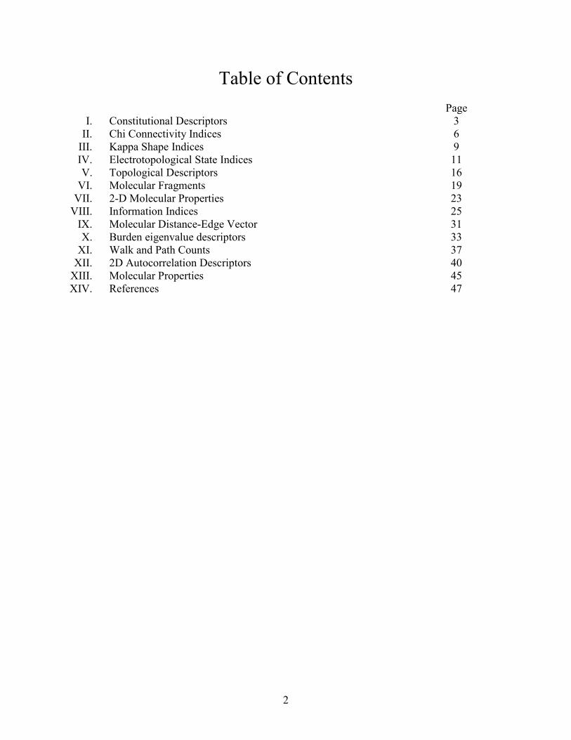
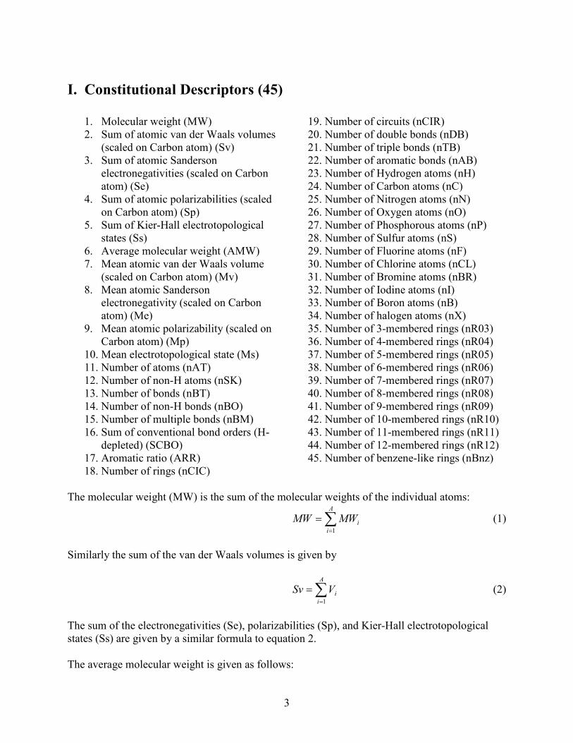
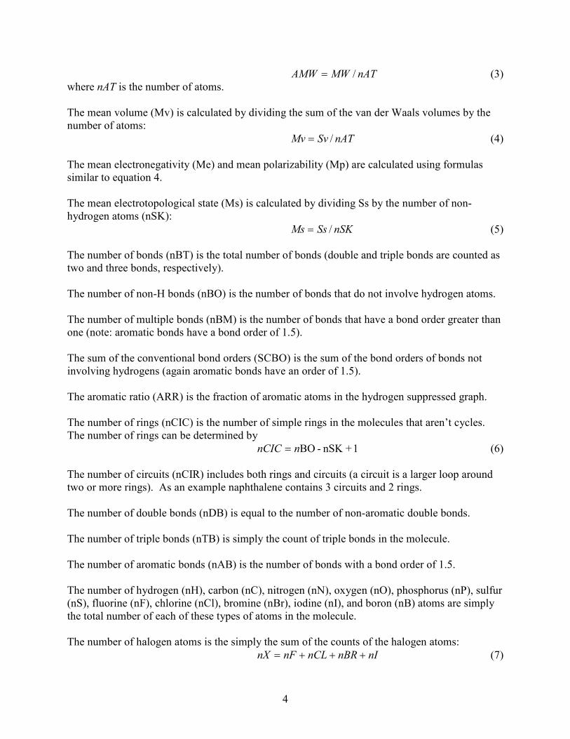
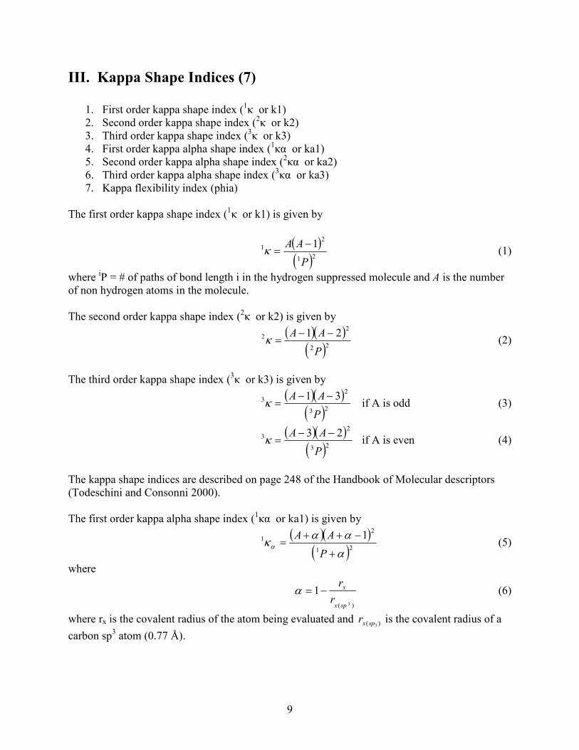
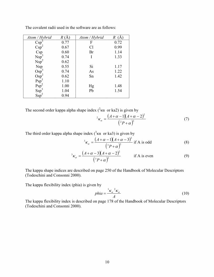
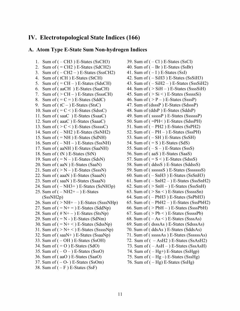
5
10
15
20
25
30
35
IV Electrotopological State Indices (166)
A Atom Type EshyState Sum Nonshyhydrogen Indices
1 Sum of ( ndash CH3 ) EshyStates (SsCH3) 2 Sum of ( = CH2 ) EshyStates (SdCH2) 3 Sum of ( ndash CH2 ndash ) EshyStates (SssCH2) 4 Sum of ( tCH ) EshyStates (StCH) Sum of ( = CH ndash ) EshyStates (SdsCH)
6 Sum of ( aaCH ) EshyStates (SaaCH) 7 Sum of ( gt CH ndash ) EshyStates (SsssCH) 8 Sum of ( = C = ) EshyStates (SddC) 9 Sum of ( tC ndash ) EshyStates (StsC)
Sum of ( = C lt ) EshyStates (SdssC) 11 Sum of ( saaC ) EshyStates (SsaaC) 12 Sum of ( aaaC ) EshyStates (SaaaC) 13 Sum of ( gt C lt ) EshyStates (SssssC) 14 Sum of ( ndash NH2 ) EshyStates (SsNH2)
Sum of ( = NH ) EshyStates (SdNH) 16 Sum of ( ndash NH ndash ) EshyStates (SssNH) 17 Sum of ( aaNH ) EshyStates (SaaNH) 18 Sum of ( tN ) EshyStates (StN) 19 Sum of ( = N ndash ) EshyStates (SdsN)
Sum of ( aaN ) EshyStates (SaaN) 21 Sum of ( gt N ndash ) EshyStates (SsssN) 22 Sum of ( aaaN ) EshyStates (SaaaN) 23 Sum of ( saaN ) EshyStates (SsaaN) 24 Sum of ( ndash NH3+ ) EshyStates (SsNH3p)
Sum of ( ndash NH2+ ndash ) EshyStates (SssNH2p)
26 Sum of ( gt NH+ ndash ) EshyStates (SsssNHp) 27 Sum of ( = N+ = ) EshyStates (SddNp) 28 Sum of ( N+ ndash ) EshyStates (StsNp) 29 Sum of ( = N shy ) EshyStates (SdNm)
Sum of ( = N+ lt ) EshyStates (SdssNp) 31 Sum of ( gt N+ lt ) EshyStates (SssssNp) 32 Sum of ( saaN+ ) EshyStates (SsaaNp) 33 Sum of ( ndash OH ) EshyStates (SsOH) 34 Sum of ( = O ) EshyStates (SdO)
Sum of ( ndash O ndash ) EshyStates (SssO) 36 Sum of ( aaO ) EshyStates (SaaO) 37 Sum of ( ndash Oshy ) EshyStates (SsOm) 38 Sum of ( ndash F ) EshyStates (SsF)
39 Sum of ( ndash Cl ) EshyStates (SsCl) 40 Sum of ( ndash Br ) EshyStates (SsBr) 41 Sum of ( ndash I ) EshyStates (SsI) 42 Sum of ( ndash SiH3 ) EshyStates (SsSiH3) 43 Sum of ( ndash SiH2 ndash ) EshyStates (SssSiH2) 44 Sum of ( gt SiH ndash ) EshyStates (SsssSiH) 45 Sum of ( gt Si lt ) EshyStates (SssssSi) 46 Sum of ( gt P ndash ) EshyStates (SsssP) 47 Sum of (dsssP ) EshyStates (SdsssP) 48 Sum of (ddsP ) EshyStates (SddsP) 49 Sum of ( sssssP ) EshyStates (SsssssP) 50 Sum of ( =PHlt ) EshyStates (SdssPH) 51 Sum of ( ndash PH2 ) EshyStates (SsPH2) 52 Sum of ( ndash PH ndash ) EshyStates (SssPH) 53 Sum of ( ndash SH ) EshyStates (SsSH) 54 Sum of ( = S ) EshyStates (SdS) 55 Sum of ( ndash S ndash ) EshyStates (SssS) 56 Sum of ( aaS ) EshyStates (SaaS) 57 Sum of ( = S lt ) EshyStates (SdssS) 58 Sum of ( ddssS ) EshyStates (SddssS) 59 Sum of ( ssssssS ) EshyStates (SssssssS) 60 Sum of ( ndash SnH3 ) EshyStates (SsSnH3) 61 Sum of ( ndash SnH2 ndash ) EshyStates (SssSnH2) 62 Sum of ( gt SnH ndash ) EshyStates (SssSnH) 63 Sum of ( gt Sn lt ) EshyStates (SssssSn) 64 Sum of ( ndash PbH3 ) EshyStates (SsPbH3) 65 Sum of ( ndash PbH2 ndash ) EshyStates (SssPbH2) 66 Sum of ( gt PbH ndash ) EshyStates (SsssPbH) 67 Sum of ( gt Pb lt ) EshyStates (SssssPb) 68 Sum of ( ndash As lt ) EshyStates (SsssAs) 69 Sum of ( dsssAs ) EshyStates (SdsssAs) 70 Sum of ( ddsAs ) EshyStates (SddsAs) 71 Sum of ( sssssAs ) EshyStates (SsssssAs) 72 Sum of ( ndash AsH2 ) EshyStates (SsAsH2) 73 Sum of ( ndash AsH ndash ) EshyStates (SssAsH) 74 Sum of ( ndash Hg+) EshyStates (SsHgp) 75 Sum of ( ndash Hg ndash) EshyStates (SssHg) 76 Sum of ( ndash Hg) EshyStates (SsHg)
11
The EshyState value for a given non hydrogen atom i in a molecule is given by its intrinsic state (Ii) plus the sum of the perturbations on that atom by all the other atoms in the molecule
A
Sk = Ik +sumΔIki (1) i =1
where the intrinsic state (Ik) is given by
(2 N )2δ v +1 I k = k (2)
δ k
where N = principal quantum number (which is equal to the elementrsquos period or row in the vperiodic table) where δ k is calculated using equation 6 from Section II (even for elements with
higher principal quantum levels)
The perturbation of atom k due to atom i is given by (Ii minus Ik )ΔIki = 2 (4)
rki where
r = d +1 (5) ki ki
where dki = is the number of bonds that separate atom k from atom i
The atom type nonshyhydrogen indices (SX) are obtained by summing the EshyState values for all the atoms of a given type t that are present in the molecule
SX =sumS (t) (6)
where S(t) is the atom EshyState value (obtained from equation 1) for an atom of type t
For example for propane the EshyStates for the individual atoms are as follows
S(2)=125
CH3H3C
S(1)=2125 S(3)=2125
SsCH3 (the sum of the EshyStates for carbon atoms with three hydrogens attached and one single bond to a nonhydrogen atom) is 425 (2times 2125) SssCH2 (the sum of the EshyStates for carbon atoms with two hydrogens attached and two single bonds to a nonhydrogen atoms) is 125
12
B Atom Type Count Nonshyhydrogen Indices
1 Count of ( ndash CH3 ) (SsCH3_acnt) 2 Count of ( = CH2 ) (SdCH2_acnt) 3 Count of ( ndash CH2 ndash ) (SssCH2_acnt) 4 Count of ( tCH ) (StCH_acnt) 5 Count of ( = CH ndash ) (SdsCH_acnt) 6 Count of ( aaCH ) (SaaCH_acnt) 7 Count of ( gt CH ndash ) (SsssCH_acnt) 8 Count of ( = C = ) (SddC_acnt) 9 Count of ( tC ndash ) (StsC_acnt) 10 Count of ( = C lt ) (SdssC_acnt) 11 Count of ( saaC ) (SsaaC_acnt) 12 Count of ( aaaC ) (SaaaC_acnt) 13 Count of ( gt C lt ) (SssssC_acnt) 14 Count of ( ndash NH2 ) (SsNH2_acnt) 15 Count of ( = NH ) (SdNH_acnt) 16 Count of ( ndash NH ndash ) (SssNH_acnt) 17 Count of ( aaNH ) (SaaNH_acnt) 18 Count of ( tN ) (StN_acnt) 19 Count of ( = N ndash ) (SdsN_acnt) 20 Count of ( aaN ) (SaaN_acnt) 21 Count of ( gt N ndash ) (SsssN_acnt) 22 Count of ( aaaN ) (SaaaN_acnt) 23 Count of ( saaN ) (SsaaN_acnt) 24 Count of ( ndash NH3+ ) (SsNH3p_acnt) 25 Count of ( ndash NH2+ ndash ) (SssNH2p_acnt) 26 Count of ( gt NH+ ndash ) (SsssNHp_acnt) 27 Count of ( = N+ = ) (SddNp_acnt) 28 Count of ( N+ ndash ) (StsNp_acnt) 29 Count of ( = N shy ) (SdNm_acnt) 30 Count of ( = N+ lt ) (SdssNp_acnt) 31 Count of ( gt N+ lt ) (SssssNp_acnt) 32 Count of ( saaN+ ) (SsaaNp_acnt) 33 Count of ( ndash OH ) (SsOH_acnt) 34 Count of ( = O ) (SdO_acnt) 35 Count of ( ndash O ndash ) (SssO_acnt) 36 Count of ( aaO ) (SaaO_acnt) 37 Count of ( ndash Oshy ) (SsOm_acnt) 38 Count of ( ndash F ) (SsF_acnt)
39 Count of ( ndash Cl ) (SsCl_acnt) 40 Count of ( ndash Br ) (SsBr_acnt) 41 Count of ( ndash I ) (SsI_acnt) 42 Count of ( ndash SiH3 ) (SsSiH3_acnt) 43 Count of ( ndash SiH2 ndash ) (SssSiH2_acnt) 44 Count of ( gt SiH ndash ) (SsssSiH_acnt) 45 Count of ( gt Si lt ) (SssssSi_acnt) 46 Count of ( gt P ndash ) (SsssP_acnt) 47 Count of (dsssP ) (SdsssP_acnt) 48 Count of (ddsP ) (SddsP_acnt) 49 Count of ( sssssP ) (SsssssP_acnt) 50 Count of ( =PHlt ) (SdssPH_acnt) 51 Count of ( ndash PH2 ) (SsPH2_acnt) 52 Count of ( ndash PH ndash ) (SssPH_acnt) 53 Count of ( ndash SH ) (SsSH_acnt) 54 Count of ( = S ) (SdS_acnt) 55 Count of ( ndash S ndash ) (SssS_acnt) 56 Count of ( aaS ) (SaaS_acnt) 57 Count of ( = S lt ) (SdssS_acnt) 58 Count of ( ddssS ) (SddssS_acnt) 59 Count of ( ssssssS ) (SssssssS_acnt) 60 Count of ( ndash SnH3 ) (SsSnH3_acnt) 61 Count of ( ndash SnH2 ndash ) (SssSnH2_acnt) 62 Count of ( gt SnH ndash ) (SssSnH_acnt) 63 Count of ( gt Sn lt ) (SssssSn_acnt) 64 Count of ( ndash PbH3 ) (SsPbH3_acnt) 65 Count of ( ndash PbH2 ndash ) (SssPbH2_acnt) 66 Count of ( gt PbH ndash ) (SsssPbH_acnt) 67 Count of ( gt Pb lt ) (SssssPb_acnt) 68 Count of ( ndash As lt ) (SsssAs_acnt) 69 Count of ( dsssAs ) (SdsssAs_acnt) 70 Count of ( ddsAs ) (SddsAs_acnt) 71 Count of ( sssssAs ) (SsssssAs_acnt) 72 Count of ( ndash AsH2 ) (SsAsH2_acnt) 73 Count of ( ndash AsH ndash ) (SssAsH_acnt) 74 Count of ( ndash Hg+) (SsHgp_acnt) 75 Count of ( ndash Hg ndash) (SssHg_acnt) 76 Count of ( ndash Hg) (SsHg_acnt)
The atom type count nonshyhydrogen indices are simply the count of each type of eshystate fragment within a molecule For the propane example SsCH3_acnt (the count of all ndash CH3 groups in molecule) is 2 and SssCH2_acnt (the count of all ndash CH2 ndash groups in a molecule) is 1
13
C Hydrogen Indices
1 Sum of ([ndash OH ]) hydrogen EshyStates (SHsOH) 2 Sum of ([= NH ]) hydrogen EshyStates (SHdNH) 3 Sum of ([ndash SH ]) hydrogen EshyStates (SHsSH) 4 Sum of ([ndash NH2]) hydrogen EshyStates (SHsNH2) 5 Sum of ([ndash NH ndash ]) hydrogen EshyStates (SHssNH) 6 Sum of ([ tCH ]) hydrogen EshyStates (SHtCH) 7 Sum of (CH or CH2 with shyF or shyCl attached) hydrogen EshyState values (SHCHnX) 8 Sum of hydrogen EshyState values for other atom types (SHother)
The hydrogen electrotopological state index ( HSi ) for atom number i is given by
KHE j minus KHE(Hi ) HSi = KHE + (KHEi minus KHE(H ))+ (7)i i sum jnei 2(d +1)ij
where KHEi is the KiershyHall electronegativity of the ith heavy atom in the Hshydepleted graph KHE(Hi ) is the KiershyHall electronegativity of the attached hydrogen atom (taken to be shy02)
and dij is the distance between each j heavy atom and the ith heavy atom to which the hydrogen is bonded The KiershyHall electronegativity of a given atom is given by
vδ minusδ KHE = i
2i (8) i
N i
vwhere in this case δ i is the valence vertex degree given in equation 6 of Section II and Ni is the
principal quantum number of atom i
SHsOH is the sum of the hydrogen EshyStates for the atoms with an EshyState type of SsOH
SHdNH is the sum of the hydrogen EshyStates for the atoms with an EshyState type of SdNH
SHsSH is the sum of the hydrogen EshyStates for the atoms with an EshyState type of SsSH
SHsNH2 is the sum of the hydrogen EshyStates for the atoms with an EshyState type of SsNH2
SHssNH is the sum of the hydrogen EshyStates for the atoms with an EshyState type of SssNH or SaaNH
SHtCH is the sum of the hydrogen EshyStates for the atoms with an EshyState type of StCH
SHCHnX is the sum of the hydrogen EshyStates for the atoms with an EshyState type of SsCH3 SssCH2 SsssCH or SdsCH when there is a chlorine or fluorine atom attached
SHother is the sum of the hydrogen EshyStates for atoms (that have hydrogens attached) that do not fall into the other hydrogen EshyState types listed above
14
D Maximum and Minimum Values
1 Maximum hydrogen EshyState value in molecule (Hmax) 2 Maximum EshyState value in molecule (Gmax) 3 Minimum hydrogen EshyState value in molecule (Hmin) 4 Minimum EshyState value in molecule (Gmin) 5 Maximum positive hydrogen EshyState value in molecule (Hmaxpos) 6 Minimum negative hydrogen EshyState value in molecule (Hminneg)
Hmax is the maximum hydrogen Eshystate value (calculated using equation 7) for all the atoms in the molecule
Gmax is the maximum Eshystate value (calculated using equation 1) for all the atoms in the molecule
Hmin is the minimum hydrogen Eshystate value for all the atoms in the molecule
Gmin is the minimum Eshystate value for all the atoms in the molecule
Hmaxpos is the maximum positive hydrogen Eshystate value for all the atoms in the molecule
Hminneg is the minimum negative hydrogen Eshystate value for all the atoms in the molecule
The calculation of Eshystates indices is described in further detail by Kier and Hall(Kier and Hall 1999)
15
V Topological descriptors (15)
1 First Zagreb index weighted by vertex degrees (ZM1) 2 First Zagreb index weighted by valence vertex degrees (ZM1V) 3 Second Zagreb index weighted by vertex degrees (ZM2) 4 Second Zagreb index weighted by valence vertex degrees (ZM2V) 5 Balaban distance connectivity index (J) 6 Jt index (Jt) 7 Balaban centric index (BAC) 8 Lopping centric index (Lop) 9 Radial centric information index (ICR) 10 EshyState topological parameter (TIE) 11 Maximal electrotopological negative variation (MAXDN) 12 Maximal electrotopological positive variation (MAXDP) 13 Molecular electrotopological variation (DELS) 14 Wiener Index (W) 15 Mean Wiener Index (WA)
The first Zagreb index (weighted by vertex degrees) is given by
ZM1 =sum δ a2 (1)
a
where a runs over the A atoms of the molecule and δ a is the vertex degree of atom a vZM1V =sum δ a
2 (2)
a
vwhere δ a is the valence vertex degree of atom a
ZM 2 = sum (δ i sdotδ j ) (3) b b
where b runs over all of the bonds in the molecule v vZM 2V = sum (δ i sdotδ j ) (4)
b b
The Zagreb indices (ZM1 ZM1V ZM2 and ZM2V) are described on pg 509 of the Handbook of Molecular descriptors (Todeschini and Consonni 2000)
The Balaban distance connectivity index (J) is given by B minus1 2
J = sum(σ iσ j )b (5)
C +1 b
where σ i and σ j are the vertex distance degrees of two adjacent atoms and the sum runs over
all the molecular bonds b B is the number of bonds and C (the cyclomatic number) is the number of rings The vertex distance degree ( σ i ) is the sum of the distances of all the other
atoms to a given atom A
σ i = sumdij (6) j=1
where dij is the topological distance between atoms i and j
16
The cyclomatic number is given by C = B minus A +1 (7)
A similar index the Jt index is defined as follows B minus1 2
J t = sum(tit j )b (8)
C +1 b
where ti is a different local vertex invariant given by σ iti = (9) δ i
J and Jt are described on pg 21 of the Handbook of Molecular descriptors (Todeschini and Consonni 2000)
To calculate the centric indices the vertices with a vertex degree of unity are stepwise removed until no more vertices can be removed The Balaban centric index is calculated as follows
R
BAC = sumng 2 (10)
g =1
where ng is the number of atoms with a vertex degree of unity removed at step g and R is the number of removal steps
The Lopping centric index is calculated as follows R ng ng
Lop = minussum log (11) i=1 A A
BAC and Lop are described on pg 42 of the Handbook of Molecular descriptors(Todeschini and Consonni 2000)
The radial centric information index (ICR) is calculated as follows G ng ng
ICR = minussum log2 (12) g minus1 A A
where ng is the number of vertices having equal atom eccentricities (η ) in the gth class G is the number of equivalence classes and A is the atom number The atom eccentricity is the maximum distance from the ith vertex to the other vertices
η i = max(dij ) (13) j
ICR is described on pg 44 of the Handbook of Molecular descriptors (Todeschini and Consonni 2000)
Voeckel (1994) defines the EshyState topological parameter (TIE) as follows B minus1 2
TIE = sum B
(Si sdot S j )b (14)
C +1 b=1
In order to match the descriptor used in Dragon (Talete 2006) (and to be able to calculate TIE for compounds with atoms with negative EshyState values) the EshyState topological parameter is instead given by
17
B minus1 2TIE = sum
B
(1+ exp(Si ) sdot exp(S j ))b (15)
C +1 b=1
where B is the number of bonds C is the cyclomatic number Si is the EshyState for atom i TIE is described on pg 165 of the Handbook of Molecular descriptors (Todeschini and Consonni 2000)
The maximal electrotopological negative variation (MAXDN) is given by MAXDN = max ΔI i if ΔI i lt 0 i = 1A (16)
i
where ΔI i is the field effect on the ith atom due to the perturbation of all other atoms
I i minus I jΔI i = sum 2 (17) (d +1)j ij
Similarly the maximal electrotopological positive variation (MAXDP) is given by MAXDP = max ΔI i if ΔI i gt 0 i = 1A (18)
i
The molecular electrotopological variation (DELS) is given by DELS ΔI i (19) = sum
i
MAXDN MAXDP and DELS are described in more detail by Gramatica (Gramatica et al 2000)
The Wiener index (W) is given by 1 A A
W = 2 sumsumdij (20)
i=1 i=1
where dij is the topological distance between atoms i and j
The mean Wiener index is given by 2W
WA = (21) A(A minus1)
W and WA are described in more detail on pg 497 of the Handbook of Molecular descriptors (Todeschini and Consonni 2000)
18
5
10
15
20
25
30
35
40
VI Molecular Fragments (234)
1 ACAC 2 AN [attached to AN in same ring] 3 ANH [attached to AN in same ring] 4 C=C=O C=[N+][Oshy]
6 C=[N+]=(Aguiara et al) 7 shyN=S=O 8 shyN=[N+]=(Aguiara et al) 9 shy[N+]N
A[N+][Oshy] 11 N+ [four single bonds] 12 CH2=C(CH3)C(=O)Oshy13 CH2=CHC(=O)Oshy14 shyN=C=S
shySC(=S)Sshy16 shySC(=S)Oshy17 shySC(=O)Sshy18 shySC(=O)Oshy19 shyOC(=S)Oshy
shyC(=O)OC(=O)shy21 shyNHshy [3 membered ring] 22 shyNlt [3 membered ring] 23 shyNH2 [attached to P] 24 shyNHshy [attached to P]
shyNlt [attached to P] 26 Sn=O 27 Sn [oxygen attach] 28 Sn [aromatic attach] 29 Sn
Si [aromatic attach] 31 Si [oxygen aromatic attach] 32 Si [oxygen attach] 33 Si 34 shyS(=O)(=O)shy [2 nitrogen attach]
shyS(=O)(=O)shy [nitrogen aromatic attach]
36 shyS(=O)(=O)shy [aromatic attach] 37 shyS(=O)(=O)shy [olefinic attach] 38 shyS(=O)(=O)shy [nitrogen aliphatic
attach] 39 shyS(=O)(=O)shy [aliphatic attach]
shyS(=O)shy [2 nitrogen attach] 41 shyS(=O)shy [nitrogen aromatic attach] 42 shyS(=O)shy [aromatic attach]
43 shyS(=O)shy olefinic attach] 44 shyS(=O)shy [nitrogen aliphatic attach] 45 shyS(=O)shy [aliphatic attach] 46 shyOH [aromatic attach] 47 shySH [aromatic attach] 48 shyN=O [aromatic attach] 49 shyONO2 50 shyNO2 [aromatic attach] 51 shyNO2 [olefinic attach] 52 shyNO2 [nitrogen attach] 53 shyNO2 [aliphatic attach] 54 shyN=C=O [aromatic attach] 55 shyN=C=O [aliphatic attach] 56 shyCOOH [aromatic attach] 57 shyOC(=O)Oshy58 shyC(=O)Oshy [aromatic attach] 59 shyC(=O)SH [aromatic attach] 60 shyC(=O)Sshy [aromatic attach] 61 shyC(=S)SH [aromatic attach] 62 shyC(=S)Sshy [aromatic attach] 63 shyC(=S)OH [aromatic attach] 64 shyC(=S)Oshy [aromatic attach] 65 shyC(=S)shy [nitrogen aromatic attach] 66 shyC(=S)shy [aromatic attach] 67 shyCHO [aromatic attach] 68 shyCOOH [aliphatic attach] 69 HC(=O)Oshy70 shyC(=O)Oshy [nitrogen attach] 71 shyC(=O)Oshy [cyclic] 72 shyC(=O)Oshy [olefinic attach] 73 shyC(=O)Oshy [aliphatic attach] 74 shyC(=O)SH [nitrogen attach] 75 shyC(=O)SH [aliphatic attach] 76 shyC(=O)Sshy [nitrogen attach] 77 shyC(=O)Sshy [aliphatic attach] 78 shyC(=S)SH [nitrogen attach] 79 shyC(=S)SH [aliphatic attach] 80 shyC(=S)OH [aliphatic attach] 81 shyC(=S)Oshy [nitrogen attach] 82 shyC(=S)Oshy [aliphatic attach] 83 shyC(=S)Sshy [nitrogen attach] 84 shyC(=S)Sshy [aliphatic attach] 85 shyC(=S)shy [2 nitrogen attach] 86 shyC(=S)shy [nitrogen aliphatic attach]
19
87 shyC(=S)shy [aliphatic attach] 88 shyCF3 [aromatic attach] 89 shyCCl3 [aromatic attach] 90 shyCN [aromatic attach] 91 shyCH=NOH 92 shyCH=NO 93 gtC=NOH 94 gtC=NO 95 shyC([H])=N[H] [Nitrogen attach] 96 shyC([H])=N [Nitrogen attach] 97 gtC=N[H] [2 Nitrogen attach] 98 gtC=N[H] [Nitrogen attach] 99 gtC(=N) [2 Nitrogen attach] 100 gtC(=N) [Nitrogen attach] 101 shyCH=NH 102 gtC=NH 103 CH2=N 104 shyCH=N 105 gtC=N 106 shyNHN=O 107 gtNN=O 108 shyN(=O) 109 shyN=NH 110 shyN=Nshy111 shyNH2 [nitrogen attach] 112 shyNHshy [nitrogen attach] 113 shyNlt [nitrogen attach] 114 shyCHO [nitrogen attach] 115 shyCHO [aliphatic attach] 116 shyC(=O)shy [halogen attach] 117 shyC(=O)shy [2 aromatic attach] 118 shyC(=O)shy [nitrogen aromatic attach] 119 shyC(=O)shy [aromatic attach] 120 shyC(=O)shy [2 nitrogen attach] 121 shyC(=O)shy [nitrogen aliphatic attach] 122 shyC(=O)shy [phosphorus attach] 123 shyC(=O)shy [olefinic attach] 124 C=O(ketone aliphatic attach) 125 C=O(nonshyketone aliphatic attach) 126 shyCCl3 [aliphatic attach] 127 shyCF3 [aliphatic attach] 128 shyCN [aliphatic nitrogen attach] 129 shyCN [aliphatic sulfur attach] 130 shyCN [olefinic attach] 131 shyCN [aliphatic attach] 132 P=NH
133 P=N 134 P=S 135 P(=O) 136 As(=O) 137 shySH [aliphatic attach] 138 shySshy [three membered ring] 139 shySshy [sulfur attach] 140 shySshy [arsenic attach] 141 shySshy [phosphorus attach] 142 shySshy [nitrogen attach] 143 shySshy [2 aromatic attach] 144 shySshy [aromatic attach] 145 shyOH [sulfur attach] 146 shyOH [oxygen attach] 147 shyOH [arsenic attach] 148 shyOH [phosphorus attach] 149 shyOH [nitrogen attach] 150 shyOH [aliphatic attach] 151 shyOshy (epoxide) 152 shyOshy [2 aromatic attach] 153 shyOshy [phosphorus aromatic attach] 154 shyOshy [2 phosphorus attach] 155 shyOshy [phosphorus attach] 156 shyOshy [arsenic attach] 157 shyOshy [nitrogen attach] 158 shyOshy [sulfur attach] 159 shyOshy [oxygen attach] 160 shyOshy [aromatic attach] 161 shyCH= [aromatic attach] 162 gtC= [aromatic attach] 163 shyC [aromatic attach] 164 shyCH3 [aromatic attach] 165 shyCH2shy [aromatic attach] 166 shyCHlt [aromatic attach] 167 gtClt [aromatic attach] 168 shyCH3 [aliphatic attach] 169 shyCH2shy [aliphatic attach] 170 shyCHlt [aliphatic attach] 171 gtClt [aliphatic attach] 172 =C= 173 =CH2 [aliphatic attach] 174 =CH [aliphatic attach] 175 =C [aliphatic attach] 176 CH [aliphatic attach] 177 C [aliphatic attach] 178 shyNH2 [aromatic attach]
20
179 shyNHshy [aromatic attach] 208 shyCl [aliphatic attach] 180 shyNlt [aromatic attach] 209 shyF [aliphatic attach] 181 shyNH2 [aliphatic attach] 210 shyI [aliphatic attach] 182 shyNHshy [aliphatic attach] 211 H [phosphorus attach] 183 shyNlt [aliphatic attach] 212 H [nitrogen attach] 184 Fused aromatic carbon 213 H [silicon attach] 185 Fused aromatic nitrogen 214 H [carbon attach] 186 ACH 215 H [other] 187 ANH 216 shyHg 188 AC 217 shyHgshy189 AN 218 shyHg+ 190 AN+ 219 Hg 191 AO 220 Pb 192 AS 221 B 193 =O [other] 222 P [+3 valence all single bonds] 194 =S [other] 223 P [+3 valence all single bonds] 195 shy[Oshy] 224 P [+3 valence all single bonds] 196 shyOshy [aliphatic attach] 225 P [+5 valence one double bond] 197 shySshy [aliphatic attach] 226 P [+5 valence two double bonds] 198 shyF [aromatic attach] 227 P [+5 valence all single bonds] 199 shyBr [aromatic attach] 228 P 200 shyCl [aromatic attach] 229 As [+3 valence one double bond] 201 shyI [aromatic attach] 230 As [+3 valence all single bonds] 202 shyBr [olefinic attach] 231 As [+5 valence one double bond] 203 shyCl [olefinic attach] 232 As [+5 valence two double bonds] 204 shyF [olefinic attach] 233 As [+5 valence all single bonds] 205 shyI [olefinic attach] 234 As 206 Halogen [Nitrogen attach] 207 shyBr [aliphatic attach]
21
The molecular fragment counts (Martin et al 2008) represent the number of times various
fragments appear in a molecule The fragments are written in a format similar to SMILES
notation (Daylight Chemical Information Systems 2006) The fragments were designed so that
each atom in a molecule is only assigned to one fragment Dashes (shy) represent single bonds
Carats (lt) represent two single bonds equal signs (=) represent double bonds and pound signs
() represent triple bonds The terms inside the brackets provide additional information such as
what the fragment is attached to For example
ldquoshyOshy [phosphorus aromatic attach]rdquo is the count of oxygen atoms that are attached to a
phosphorus atom and an aromatic atom The phosphorus atom and the aromatic atom are not
considered to be part of the fragment In addition the term inside the brackets can indicate
whether the fragment is part of a ring (for example
ldquoshySshy [three membered ring]rdquo) or indicate the valence state of a given element (for example ldquoAs
[+3 valence one double bond]rdquo) The fragments are assigned in the order that they appear
above For example 12shydichlorobenzene would have the following fragment counts
shyCl [aromatic attach] = 2 AC = 2 and ACH = 4
22
VII 2shyD Molecular Properties (9)
1 Number of hydrogen bond acceptors (numHBa) 2 Number of hydrogen bond donors (numHBd) 3 Number of weak hydrogen bond donors (ie ndashCHX where X = Cl F) (numwHBd) 4 Sum of EshyState indices for hydrogen bond acceptors (SHHBa) 5 Sum of EshyState indices for hydrogen bond donors (SHHBd) 6 Sum of EshyState indices for weak hydrogen bond donors (SHwHBd) 7 Molecular and group polarity index (Qs) 8 Molecular and group polarity index (Qv) 9 Average of Qs and Qv (Qsv)
The number of hydrogen bond acceptors (numHBa) is the total count of fluorine oxygen nonaromatic nitrogens and aromatic nitrogens with an Eshystate fragment of SaaN (pyrrolyl nitrogens are not considered to be hydrogen bond acceptors)
The number of hydrogen bond donors (numHBd) is the total count of hydrogens that are attached to oxygen or nitrogen atoms
The number of weak hydrogen bond donors (numwHBd) is the count of carbon atoms that have both a hydrogen atom and a chlorine or fluorine atom attached
The sum of EshyState indices for hydrogen bond acceptors (SHHBa) is the sum of the Eshystate indices for atoms that are assigned to be hydrogen bond acceptors
The sum of EshyState indices for hydrogen bond donors (SHHBd) is the sum of the hydrogen Eshystate indices for oxygens and nitrogens
The sum of the EshyState indices for weak hydrogen bond donors (SHwHBd) is the sum of the hydrogen EshyStates for the carbon atoms that have both a hydrogen and a chlorine or fluorine attached
The Qs molecular and group polarity index is given by A
2 alkaneA sum I i i=1Qs =
2 (1)
sum A I i i=1
where Iialkane = The intrinsic state value of an atom considering all nonshyhydrogen atoms have
been replaced by sp3 carbon atoms (keeping the same isoconnectivity)
The Qv molecular and group polarity index is given by A A
max alkanesum I i sum I i i=1 i=1Q =
2 (2) v
sum A I i i=1
23
where Iimax = The intrinsic state value of the atom where the following replacements have been
made (a) all terminal atoms (atoms bonded to one other nonshyhydrogen atom) replaced by
ndashF (I = 8000) (b) all divalent atoms (atoms bonded to two other nonshyhydrogen atoms) replaced by
ndashOshy (I = 3500) (c) all trivalent atoms (atoms bonded to three other nonshyhydrogen atoms) replaced by
gtNshy (I = 2000) (d) all quaternary atoms (atoms bonded to four other nonshyhydrogen atoms) replaced by
gtClt (I = 1250)
The average of Qs and Qv is given by A A
ave alkanesum I sum Ii i
svQ = 1=i2
1
1
sum
=
=
A
i i
i
I
(3)
whereA A
1 sum =
A
i
ave iI =
2 1
max
1 + sumsum
== i i
i
alkane i II
(4)
The equations for Qs Qv and Qsv were taken from documentation for MDL QSAR (Elsevier_MDL 2006)
24
VIII Information Indices (36)
A Connectivity Based (8) 1 Information bond index (ib)
2 Mean information content on the edge magnitude (eim)
3 Information content (ic)
4 Mean information content or Shannonrsquos entropy (si)
5 Total information content (I) 6 Maximum information content (maxIC or maxic) 7 Standardized Shannon Information or standardized information content (ssi) 8 Brillouin redundancy index (R)
The information bond index is given by B
ib = B log2 ( ) B minus G
sum Bg log2 (Bg ) (1) g =1
where B = the number of bonds in the molecule Bg = the number of bonds of type g in the molecule and GB = all of the different bond types in the molecule
The mean information content on the edge magnitude (eim) is based on the magnitude of edge connectivities and is given by
minus1 2 minus1 2(δ δ )b
(δ δ )b
i j i j
eim = minussum B
1 log2
1
(2)
b=1 χ χ minus1 2where 1χ is the first order Chi connectivity index (x1 in Section I) (δ iδ j ) is the edge b
connectivity of the b bond and B is the number of bonds
The information content (a measure of molecular symmetry) of a system having n elements is given by
G ic = sum ng log2 (ng ) (3)
g =1
where ng is the number of topologically equivalent atoms of type g and G is the number of topologically different atom types The information content is the same as the zeroth order kappa shape index or Kier symmetry index (Kier 1987) Each equivalence type is constituted by all atoms having the same valence topological state (Sv) The valence topological state is given by
A vSvi = sum tij (4)
iminus1
where tijv is the valence topological state matrix given by
v v tij = GM ij (1 nij ) (5)
25
where nij is the number of atoms in the path of mth order GMij
v is the geometric mean of the
valence vertex degree of the atoms involved in the path between atoms i and j of length m and is defined as
1 ijnij n
v vGM ij = prodδ a
(6) a=1
The mean information content is defined as follows G
si = minussum p log (p ) (7) g 2 g g =1
where pg = the probability (ngn) of selecting the gth topological equivalent type For molecules the total number of elements in the system (n) is the same as A (the number of nonshyhydrogen atoms)
The total information content (I) is obtained by multiplying the mean information content by the number of elements
I = n sdot si (8)
The maximum information content (maxic) represents the information content needed to characterize all of the n alternatives
maxic = n log2 (n) (9)
The standardized information content (ssi) is the ratio between the total information content and the maximum information content
I ssi = (10)
maxic
Brillouin redundancy index (R) a measure of the information redundancy of a system is given by R = 1minus ssi (11)
The connectivity based information indices are described in more detail on pages 238shy240 of the Handbook of Molecular Descriptors (Todeschini and Consonni 2000)
Topologically Based (28) V E1 Total information content on the adjacency equality ( I adj or iadje) V E2 Mean information content on the adjacency equality ( Iadj or iadjem)
V M3 Total information content on the adjacency magnitude ( Iadj or iadjm) V M4 Mean information content on the adjacency magnitude ( Iadj or iadjmm)
5 Mean information content of the vertex degree equality ( V I E or ivdem) adj deg
6 Mean information content of the vertex degree magnitude ( V I M or ivdmm) adj deg
E E7 Total information content on the edge adjacency equality ( Iadj or ieadje) E E8 Mean information content on the edge adjacency equality ( Iadj or ieadjem)
26
9 Total information content on the edge adjacency magnitude ( E I M or ieadjm) adj
10 Mean information content on the edge adjacency magnitude ( E I M or ieadjmm) adj
11 Total information content on the distance equality ( V ID
E or ide)
12 Mean information content on the distance equality ( V ID
E or idem)
13 Total information content on the distance magnitude ( V ID
M or idm)
14 Mean information content on the distance magnitude ( V ID
M or idmm)
15 Mean information content on the distance degree equality ( V I E or iddem) Ddeg
16 Mean information content on the distance degree magnitude ( V ID
M
deg or iddmm)
17 Total information content on the edge distance equality ( EID
E or iede)
18 Mean information content on the edge distance equality ( E ID
E or iedem) 19 Edge wiener index (We) 20 Total information content on the edge distance magnitude ( EID
M or iedm)
21 Mean information content on the edge distance magnitude ( EID
M or iedmm) 22 Total vertex cyclicity (tvc) 23 Total information on the vertex cycle matrix equality ( V I E or icyce) cyc
24 Mean information on the vertex cycle matrix equality ( V I E or icycem) cyc
V M25 Total information on the vertex cycle matrix magnitude ( Icyc or icycm) V M26 Mean information on the vertex cycle matrix magnitude ( Icyc or icycmm)
27 Total topological index (tti) 28 Total topological valence index (ttvi)
The total information content on the adjacency equality (iadje) is given by 2 2 2 2iadje = A log (A )minus 2B log (2B)minus (A minus 2B)log (A minus 2B) (12) 2 2 2
The mean information content on the adjacency equality (iadjem) is given by 2B 2B 2B 2B
iadjem = minus log2 minus 1minus log2 1minus (13) 2 2 2 2A A A A
where A = the number of nonshyhydrogen atoms in molecule (same as above) and B = the number of bonds in the molecule (same as above) The elements of the Adjacency Matrix aij equal 1 if the ith atom and the jth atom are bonded together and equal 0 if not
The total information content on the adjacency magnitude (iadjm) is given by iadjm = 2B log2 (2B) (14)
The mean information content on the adjacency magnitude (iadjmm) is given by iadjmm = 1+ log2 (B) (15)
The mean information content of the vertex degree equality (ivdem) is given by
27
G g gF F ivdem = minussum log (16)2
g minus1 A A g F is the number of vertices with vertex degree equal to g
The mean information content of the vertex degree magnitude (ivdmm) is given by G
g ivdmm = minussum F
g log2
g (17)
g minus1 2B 2B
The total information content on the edge adjacency equality (ieadje) is given by 2 2 2 2ieadje = B log (B )minus 2N log (2N )minus (B minus 2N )log (B minus 2N 2 ) (18) 2 2 2 2 2 2
The mean information content on the edge adjacency equality (ieadjem) is given by 2N 2 2N 2 2N 2 2N 2 ieadjem = minus log minus 1minus log 1minus (19)
2 2 2 2B2 B B
2 B
where N2 = the number of 2nd order path counts in the molecule
The total information content on the edge adjacency magnitude (ieadjm) is given by ieadjm = 2N 2 log2 (2N 2 ) (20)
The mean information content on the edge adjacency magnitude (ieadjmm) is given by ieadjmm = 1+ log2 (N 2 ) (21)
The total information content on the distance equality (ide) is given by GA(A minus1) A(A minus1) g gide = log2 minussum f log2 ( f ) (22)
2 2 g =1
g fwhere is the number of distances with equal g values in the triangular D submatrix D is an A x A matrix that contains the graph distances between atoms The graph distances are calculated as 1(the of bonds between atoms)2
The mean information content on the distance equality (idem) is given by g gG 2sdot f 2sdot f
idem = minussum log (23) 2 )g =1 A(A minus1) A(A minus1 The total information content on the distance magnitude (idm) is given by
gW log ( )minus sum f sdot g log2 gidm = 2 W ( ) (24)
The mean information content on the distance magnitude (idmm) is given by G
g idmm = minussum f sdot
g log2
g (25)
g =1 W W
The mean information content on the distance degree equality (iddem)
28
G n n iddem = minussum g
log2 g
(26) g minus1 A A
where ng is the number of vertices having equal vertex distance degrees (σ ) in the gth class G is the number of equivalence classes
The mean information content on the distance degree magnitude (iddmm) is given by G σ g σ g
iddmm = minussumng log2 (27) g minus1 2W 2W
The total information content on the edge distance equality (iede) is given by B(B minus1) B(B minus1) g giede = log2 minus sum f log2 ( f ) (28)
2 2
The mean information content on the edge distance equality (iedem) is given by g g2sdot f 2sdot f
iedem = minussum log2 (29) B(B minus1)
B(B minus1)
The edge wiener index (We) is given by A(A minus1)
We = W minus (30) 2
The total information content on the edge distance magnitude (iedm) is given by gWe log ( )minus sum f sdot g log2 giedm = 2 We ( ) (31)
The mean information content on the edge distance magnitude (iedmm) is given by
g g g iedmm = minussum f sdot log2 (32)
We We
The total vertex cyclicity (tvc) is given by A C+
tvc = sum sum cij (33) i=1 j=1
where C+ = the number of cycles in a molecule (eg Naphthalene has 3 cycles) and cij = 1 if the ith atom is part of the jth cycle and 0 otherwise The elements cij comprise the vertex cycle matrix CV
The total information on the vertex cycle matrix equality (icyce) is given by + +icyce = A sdot C log (A sdot C )minus n log (n )minus n log (n0 ) (34) 2 1 2 1 0 2
where n0 = the total number of cij elements that are equal to 0 and n1 = the total number of cij elements that are equal to 1
The mean information on the vertex cycle matrix equality (icycem) is given by
29
n n n n 1 1 0 0icycem = minus log minus log (35) + 2 + + 2 +A sdot C A sdot C A sdot C A sdot C
The total information on the vertex cycle matrix magnitude (icycm) is given by icycm = n1 log2 (n1 ) (36)
The mean information on the vertex cycle matrix magnitude (icycmm) is given by icycmm = log2 (n1 ) (37)
The total topological index (tti) is given by A Aminus1 A
tti = sum t + sum sum t (38) ii ij i=1 i=1 j=i+1
where t = GM sdot (1 n ) (39) ij ij ij
where GMij is the geometric mean of the vertex degree of the atoms involved in the path ishyj of length m
1 ijn n
GM = prod ij
δ (40) ij a=1
a
where δa is the vertex degree of atom a (defined in Section II) and nij = the number of atoms in the path from atom i to atom j
The total topological valence index (ttvi) is given by
A Aminus1 A v vttiv = sum tii +sum sum tij (41)
i=1 i=1 j=i+1
where the elements of the valence topological state matrix are calculated using equations 5 and 6 The topologically based information indices are described in greater detail on pages 447shy457 of the Handbook of Molecular Descriptors (Todeschini and Consonni 2000)
30
IX Molecular DistanceshyEdge Vector (19)
1 Molecular distance edge between all primary carbons (MDEC11)
2 Molecular distance edge between all primary and secondary carbons (MDEC12)
3 Molecular distance edge between all primary and tertiary carbons (MDEC13)
4 Molecular distance edge between all primary and quaternary carbons (MDEC14)
5 Molecular distance edge between all secondary carbons (MDEC22)
6 Molecular distance edge between all secondary and tertiary carbons (MDEC23)
7 Molecular distance edge between all secondary and quaternary carbons (MDEC24)
8 Molecular distance edge between all tertiary carbons (MDEC33)
9 Molecular distance edge between all tertiary and quaternary carbons (MDEC34)
10 Molecular distance edge between all quaternary carbons (MDEC44)
11 Molecular distance edge between all primary oxygens (MDEO11)
12 Molecular distance edge between all primary and secondary oxygens (MDEO12)
13 Molecular distance edge between all secondary oxygens (MDEO22)
14 Molecular distance edge between all primary nitrogens (MDEN11)
15 Molecular distance edge between all primary and secondary nitrogens (MDEN12)
16 Molecular distance edge between all primary and tertiary nitrogens (MDEN13)
17 Molecular distance edge between all secondary nitrogens (MDEN22)
18 Molecular distance edge between all secondary and tertiary nitrogens (MDEN23)
19 Molecular distance edge between all tertiary nitrogens (MDEN33)
The general formula for the molecule distance edge vector descriptors is as follows
nstλ = 2
(1) st dst
where λst is the molecular distanceshyedge vector between atom types s and t nst is the number of
possible atom pairs for a fixed combination of s and t and dst is given by
1 2sdotn )std st =prodslet (di(s) j (t ) ) ( (2)
where d is the distance (the shortest path length) between atom i with types s and atom j i(s) j (t )
with type t The geometric mean takes into account all the distances between carbon atoms i and j of types s and t The descriptors are denoted as MDEXst where X is the element s is the first atom type and t is the second atom type The atom type or degree (primary secondary or tertiary) is determined from the count of nonshyhydrogen atoms that are attached to a given atom
31
The molecular distance edge vectors are described on page 116 of the Handbook of Molecular Descriptors (Todeschini and Consonni 2000)
32
X Burden Eigenvalue Descriptors (64)
1 Highest eigenvalue n 1 of Burden matrix weighted by atomic masses (BEHm1)
2 Highest eigenvalue n 2 of Burden matrix weighted by atomic masses (BEHm2)
3 Highest eigenvalue n 3 of Burden matrix weighted by atomic masses (BEHm3)
4 Highest eigenvalue n 4 of Burden matrix weighted by atomic masses (BEHm4)
5 Highest eigenvalue n 5 of Burden matrix weighted by atomic masses (BEHm5)
6 Highest eigenvalue n 6 of Burden matrix weighted by atomic masses (BEHm6)
7 Highest eigenvalue n 7 of Burden matrix weighted by atomic masses (BEHm7)
8 Highest eigenvalue n 8 of Burden matrix weighted by atomic masses (BEHm8)
9 Lowest eigenvalue n 1 of Burden matrix weighted by atomic masses (BELm1)
10 Lowest eigenvalue n 2 of Burden matrix weighted by atomic masses (BELm2)
11 Lowest eigenvalue n 3 of Burden matrix weighted by atomic masses (BELm3)
12 Lowest eigenvalue n 4 of Burden matrix weighted by atomic masses (BELm4)
13 Lowest eigenvalue n 5 of Burden matrix weighted by atomic masses (BELm5)
14 Lowest eigenvalue n 6 of Burden matrix weighted by atomic masses (BELm6)
15 Lowest eigenvalue n 7 of Burden matrix weighted by atomic masses (BELm7)
16 Lowest eigenvalue n 8 of Burden matrix weighted by atomic masses (BELm8)
17 Highest eigenvalue n 1 of Burden matrix weighted by atomic van der Waals volumes (BEHv1)
18 Highest eigenvalue n 2 of Burden matrix weighted by atomic van der Waals volumes (BEHv2)
19 Highest eigenvalue n 3 of Burden matrix weighted by atomic van der Waals volumes (BEHv3)
20 Highest eigenvalue n 4 of Burden matrix weighted by atomic van der Waals volumes (BEHv4)
21 Highest eigenvalue n 5 of Burden matrix weighted by atomic van der Waals volumes (BEHv5)
22 Highest eigenvalue n 6 of Burden matrix weighted by atomic van der Waals volumes (BEHv6)
23 Highest eigenvalue n 7 of Burden matrix weighted by atomic van der Waals volumes (BEHv7)
33
24 Highest eigenvalue n 8 of Burden matrix weighted by atomic van der Waals volumes (BEHv8)
25 Lowest eigenvalue n 1 of Burden matrix weighted by atomic van der Waals volumes (BELv1)
26 Lowest eigenvalue n 2 of Burden matrix weighted by atomic van der Waals volumes (BELv2)
27 Lowest eigenvalue n 3 of Burden matrix weighted by atomic van der Waals volumes (BELv3)
28 Lowest eigenvalue n 4 of Burden matrix weighted by atomic van der Waals volumes (BELv4)
29 Lowest eigenvalue n 5 of Burden matrix weighted by atomic van der Waals volumes (BELv5)
30 Lowest eigenvalue n 6 of Burden matrix weighted by atomic van der Waals volumes (BELv6)
31 Lowest eigenvalue n 7 of Burden matrix weighted by atomic van der Waals volumes (BELv7)
32 Lowest eigenvalue n 8 of Burden matrix weighted by atomic van der Waals volumes (BELv8)
33 Highest eigenvalue n 1 of Burden matrix weighted by atomic Sanderson electronegativities (BEHe1)
34 Highest eigenvalue n 2 of Burden matrix weighted by atomic Sanderson electronegativities (BEHe2)
35 Highest eigenvalue n 3 of Burden matrix weighted by atomic Sanderson electronegativities (BEHe3)
36 Highest eigenvalue n 4 of Burden matrix weighted by atomic Sanderson electronegativities (BEHe4)
37 Highest eigenvalue n 5 of Burden matrix weighted by atomic Sanderson electronegativities (BEHe5)
38 Highest eigenvalue n 6 of Burden matrix weighted by atomic Sanderson electronegativities (BEHe6)
39 Highest eigenvalue n 7 of Burden matrix weighted by atomic Sanderson electronegativities (BEHe7)
40 Highest eigenvalue n 8 of Burden matrix weighted by atomic Sanderson electronegativities (BEHe8)
41 Lowest eigenvalue n 1 of Burden matrix weighted by atomic Sanderson electronegativities (BELe1)
42 Lowest eigenvalue n 2 of Burden matrix weighted by atomic Sanderson electronegativities (BELe2)
34
43 Lowest eigenvalue n 3 of Burden matrix weighted by atomic Sanderson electronegativities (BELe3)
44 Lowest eigenvalue n 4 of Burden matrix weighted by atomic Sanderson electronegativities (BELe4)
45 Lowest eigenvalue n 5 of Burden matrix weighted by atomic Sanderson electronegativities (BELe5)
46 Lowest eigenvalue n 6 of Burden matrix weighted by atomic Sanderson electronegativities (BELe6)
47 Lowest eigenvalue n 7 of Burden matrix weighted by atomic Sanderson electronegativities (BELe7)
48 Lowest eigenvalue n 8 of Burden matrix weighted by atomic Sanderson electronegativities (BELe8)
49 Highest eigenvalue n 1 of Burden matrix weighted by atomic polarizabilities (BEHp1)
50 Highest eigenvalue n 2 of Burden matrix weighted by atomic polarizabilities (BEHp2)
51 Highest eigenvalue n 3 of Burden matrix weighted by atomic polarizabilities (BEHp3)
52 Highest eigenvalue n 4 of Burden matrix weighted by atomic polarizabilities (BEHp4)
53 Highest eigenvalue n 5 of Burden matrix weighted by atomic polarizabilities (BEHp5)
54 Highest eigenvalue n 6 of Burden matrix weighted by atomic polarizabilities (BEHp6)
55 Highest eigenvalue n 7 of Burden matrix weighted by atomic polarizabilities (BEHp7)
56 Highest eigenvalue n 8 of Burden matrix weighted by atomic polarizabilities (BEHp8)
57 Lowest eigenvalue n 1 of Burden matrix weighted by atomic polarizabilities (BELp1)
58 Lowest eigenvalue n 2 of Burden matrix weighted by atomic polarizabilities (BELp2)
59 Lowest eigenvalue n 3 of Burden matrix weighted by atomic polarizabilities (BELp3)
60 Lowest eigenvalue n 4 of Burden matrix weighted by atomic polarizabilities (BELp4)
61 Lowest eigenvalue n 5 of Burden matrix weighted by atomic polarizabilities (BELp5)
62 Lowest eigenvalue n 6 of Burden matrix weighted by atomic polarizabilities (BELp6)
63 Lowest eigenvalue n 7 of Burden matrix weighted by atomic polarizabilities (BELp7)
64 Lowest eigenvalue n 8 of Burden matrix weighted by atomic polarizabilities (BELp8)
The Burden eigenvalue descriptors are determined by solving the following general eigenvalue equation
B sdotV = V sdot e (1)
where B is a real connectivity matrix to be defined V is a matrix of eigenvectors and e is a diagonal matrix of eigenvalues The rules defining B are as follows
a Hydrogen atoms are included
35
b The diagonal elements of B Bii are either given by the carbon normalized atomic mass van der Waals volume Sanderson electronegativity and polarizability of atom i
c The element of B connecting atoms i and j Bij is equal to the square root of the bond order between atoms i and j
d All other elements of B (corresponding non bonded atom pairs) are set to 0001
The carbon normalized weights used in the software as follows
Symbol Mass VdW Volume Electronegativity Polarizability C 1000 1000 1000 1000 H 0084 0299 0942 0381 N 1167 0695 1160 0625 O 1332 0512 1327 0455 P 2579 1181 0916 2063 S 2670 1088 1076 1648 F 1582 0410 1455 0318 Cl 2952 1000 1265 1239 Br 6653 1384 1171 1733 I 10566 1728 1011 3040 Si 2339 1424 0778 3057 As 6238 1181 1025 2449 Sn 9884 2041 0836 4375 Hg 16702 0695 0800 3239 Pb 17252 1538 0833 3864
The lowest eigenvalues are the absolute values of the negative eigenvalues The highest eigenvalues are the eight largest positive eigenvalues A routine for solving for eigenvalues is found in the Jama Java package (National_Institute_of_Standards_and_Technology 2005) The Burden eigenvalues descriptors are described on pages 132shy133 of the Handbook of Molecular Descriptors(Todeschini and Consonni 2000)
36
1 Molecular walk count of order 01 (MWC01) 2 Molecular walk count of order 02 (MWC02) 3 Molecular walk count of order 03 (MWC03) 4 Molecular walk count of order 04 (MWC04) 5 Molecular walk count of order 05 (MWC05) 6 Molecular walk count of order 06 (MWC06) 7 Molecular walk count of order 07 (MWC07) 8 Molecular walk count of order 08 (MWC08) 9 Molecular walk count of order 09 (MWC09) 10 Molecular walk count of order 10 (MWC10) 11 Total walk count(TWC) 12 Selfshyreturning walk count of order 01 (SRW01) 13 Selfshyreturning walk count of order 02 (SRW02) 14 Selfshyreturning walk count of order 03 (SRW03) 15 Selfshyreturning walk count of order 04 (SRW04) 16 Selfshyreturning walk count of order 05 (SRW05) 17 Selfshyreturning walk count of order 06 (SRW06) 18 Selfshyreturning walk count of order 07 (SRW07) 19 Selfshyreturning walk count of order 08 (SRW08) 20 Selfshyreturning walk count of order 09 (SRW09) 21 Selfshyreturning walk count of order 10 (SRW10) 22 Molecular path count of order 01 (MPC01) 23 Molecular path count of order 02 (MPC02) 24 Molecular path count of order 03 (MPC03) 25 Molecular path count of order 04 (MPC04) 26 Molecular path count of order 05 (MPC05) 27 Molecular path count of order 06 (MPC06) 28 Molecular path count of order 07 (MPC07) 29 Molecular path count of order 08 (MPC08) 30 Molecular path count of order 09 (MPC09) 31 Molecular path count of order 10 (MPC10) 32 Total path count(TPC) 33 Molecular multiple path count of order 01 (piPC01) 34 Molecular multiple path count of order 02 (piPC02) 35 Molecular multiple path count of order 03 (piPC03) 36 Molecular multiple path count of order 04 (piPC04) 37 Molecular multiple path count of order 05 (piPC05) 38 Molecular multiple path count of order 06 (piPC06) 39 Molecular multiple path count of order 07 (piPC07) 40 Molecular multiple path count of order 08 (piPC08) 41 Molecular multiple path count of order 09 (piPC09) 42 Molecular multiple path count of order 10 (piPC10) 43 Conventional bondshyorder ID number(piID) 44 Randic ID number(CID)
XI Walk and Path Counts (34)
37
45 Average Randic ID number(CID2) 46 Balaban ID number(BID)
The molecular walk count of kth order (MWCk) is the total number of walks of the kth length in the hydrogen suppressed molecular graph given by
A A (k )MWCk =
1 sdotsumsum aij (1)
2 i=1 j=1
where aij
(k ) are the elements of Ak (the kth power of the adjacency matrix A) and A is the number
of atoms To match Dragon (Talete 2006) the following formula was used if k is greater than one
A A (k )MWCk = ln
sumsum aij +1
(2)
i=1 j=1 The molecular walk count descriptors are described on page 481 of the Handbook of Molecular Descriptors(Todeschini and Consonni 2000)
The total walk count (TWC) is given by Aminus1 Aminus1
TWC = sumMWCk = A +sumMWCk (3) k =0 k =1
To match Dragon the following formula must be used 10
TWC = A +sumMWCk (4) k =1
The selfshyreturning walk count of kth order (SRWk) is the total number of selfshyreturning walks of length k in the graph and calculated as follows
SRWk=tr(Ak) (5) where tr is the trace operator (sum of the diagonal elements) and Ak is the kth power of the adjacency matrix The selfshyreturning walk count descriptors are described on page 384 of the Handbook of Molecular Descriptors(Todeschini and Consonni 2000)
The molecular path counts (MPCk) are simply the number of unique paths of length k The molecular path count descriptors are described on page 345 of the Handbook of Molecular Descriptors(Todeschini and Consonni 2000)
The total path count (TPC) is obtained by summing all the molecular path counts L L
TPC =sumMPCk = A +sumMPCk (6) i=0 k =1
where L is the maximum path length In order to match Dragon the total path count is instead given by
L
TPC = A +sum ln(1+ MPCk) (7) k =1
The molecular multiple path counts (piPCk) are defined as path counts weighted by the bond order
38
piPCk =sum wij (8) k pij
where k p
ij denotes a path of length k from vertex i to vertex j and wij is the path weight given by
the product of the bond orders in the path k
wij = prodπ b
(9) b=1
It should be noted that aromatic bonds are assigned a bond order of 15 In order to match Dragon again a similar logarithmic transformation is used to calculate piPCk
piPCk = ln(1+sum ij) (10) k w
pij
The conventional bondshyorder ID number(piID) is calculated as the sum of the molecular multiple path counts
L L
piID =sum piPCk = A +sum piPCk (11) k =0 k =1
The Randic ID number is also defined as a weighted molecular path count CID = A k wij (12) +sum pij
where A is the number of atoms k p
ij denotes a path of length k from vertex i to vertex j and wij is
the path weight given by minus1 2m
wij = prod(δb(1) sdotδb(2) ) (13) b=1 b
where δ and δ are the vertex degree of the two atoms incident to the bth edge and b runs b(1) b(2)
over all of the m edges of the path
The average Randic ID number is given by CID2 = CID A (14)
The Balaban ID number (BID) is calculated using the same formula as Randic ID number (CID) except the path weight is given by
minus1 2
w = m
(σ sdotσ ) (15) ij prod b(1) b(2) b=1 b
where σ and σ are the vertex distance degrees of the two atoms incident to the bth edge and b(1) b(2)
b runs over all of the m edges of the path
CID and BID are described on pages 227 and 229 respectively of the Handbook of Molecular Descriptors (Todeschini and Consonni 2000)
39
1 BrotoshyMoreau autocorrelation of a topological structure shy lag 1 weighted by atomic
masses (ATS1m) 2 BrotoshyMoreau autocorrelation of a topological structure shy lag 2 weighted by atomic
masses (ATS2m) 3 BrotoshyMoreau autocorrelation of a topological structure shy lag 3 weighted by atomic
masses (ATS3m) 4 BrotoshyMoreau autocorrelation of a topological structure shy lag 4 weighted by atomic
masses (ATS4m) 5 BrotoshyMoreau autocorrelation of a topological structure shy lag 5 weighted by atomic
masses (ATS5m) 6 BrotoshyMoreau autocorrelation of a topological structure shy lag 6 weighted by atomic
masses (ATS6m) 7 BrotoshyMoreau autocorrelation of a topological structure shy lag 7 weighted by atomic
masses (ATS7m) 8 BrotoshyMoreau autocorrelation of a topological structure shy lag 8 weighted by atomic
masses (ATS8m) 9 BrotoshyMoreau autocorrelation of a topological structure shy lag 1 weighted by atomic van
der Waals volumes (ATS1v) 10 BrotoshyMoreau autocorrelation of a topological structure shy lag 2 weighted by atomic van
der Waals volumes (ATS2v) 11 BrotoshyMoreau autocorrelation of a topological structure shy lag 3 weighted by atomic van
der Waals volumes (ATS3v) 12 BrotoshyMoreau autocorrelation of a topological structure shy lag 4 weighted by atomic van
der Waals volumes (ATS4v) 13 BrotoshyMoreau autocorrelation of a topological structure shy lag 5 weighted by atomic van
der Waals volumes (ATS5v) 14 BrotoshyMoreau autocorrelation of a topological structure shy lag 6 weighted by atomic van
der Waals volumes (ATS6v) 15 BrotoshyMoreau autocorrelation of a topological structure shy lag 7 weighted by atomic van
der Waals volumes (ATS7v) 16 BrotoshyMoreau autocorrelation of a topological structure shy lag 8 weighted by atomic van
der Waals volumes (ATS8v) 17 BrotoshyMoreau autocorrelation of a topological structure shy lag 1 weighted by atomic
Sanderson electronegativities (ATS1e) 18 BrotoshyMoreau autocorrelation of a topological structure shy lag 2 weighted by atomic
Sanderson electronegativities (ATS2e) 19 BrotoshyMoreau autocorrelation of a topological structure shy lag 3 weighted by atomic
Sanderson electronegativities (ATS3e) 20 BrotoshyMoreau autocorrelation of a topological structure shy lag 4 weighted by atomic
Sanderson electronegativities (ATS4e) 21 BrotoshyMoreau autocorrelation of a topological structure shy lag 5 weighted by atomic
Sanderson electronegativities (ATS5e) 22 BrotoshyMoreau autocorrelation of a topological structure shy lag 6 weighted by atomic
Sanderson electronegativities (ATS6e)
XII 2D Autocorrelation Descriptors
40
23 BrotoshyMoreau autocorrelation of a topological structure shy lag 7 weighted by atomic Sanderson electronegativities (ATS7e)
24 BrotoshyMoreau autocorrelation of a topological structure shy lag 8 weighted by atomic Sanderson electronegativities (ATS8e)
25 BrotoshyMoreau autocorrelation of a topological structure shy lag 1 weighted by atomic polarizabilities (ATS1p)
26 BrotoshyMoreau autocorrelation of a topological structure shy lag 2 weighted by atomic polarizabilities (ATS2p)
27 BrotoshyMoreau autocorrelation of a topological structure shy lag 3 weighted by atomic polarizabilities (ATS3p)
28 BrotoshyMoreau autocorrelation of a topological structure shy lag 4 weighted by atomic polarizabilities (ATS4p)
29 BrotoshyMoreau autocorrelation of a topological structure shy lag 5 weighted by atomic polarizabilities (ATS5p)
30 BrotoshyMoreau autocorrelation of a topological structure shy lag 6 weighted by atomic polarizabilities (ATS6p)
31 BrotoshyMoreau autocorrelation of a topological structure shy lag 7 weighted by atomic polarizabilities (ATS7p)
32 BrotoshyMoreau autocorrelation of a topological structure shy lag 8 weighted by atomic polarizabilities (ATS8p)
33 Moran autocorrelation shy lag 1 weighted by atomic masses (MATS1m) 34 Moran autocorrelation shy lag 2 weighted by atomic masses (MATS2m) 35 Moran autocorrelation shy lag 3 weighted by atomic masses (MATS3m) 36 Moran autocorrelation shy lag 4 weighted by atomic masses (MATS4m) 37 Moran autocorrelation shy lag 5 weighted by atomic masses (MATS5m) 38 Moran autocorrelation shy lag 6 weighted by atomic masses (MATS6m) 39 Moran autocorrelation shy lag 7 weighted by atomic masses (MATS7m) 40 Moran autocorrelation shy lag 8 weighted by atomic masses (MATS8m) 41 Moran autocorrelation shy lag 1 weighted by atomic van der Waals volumes (MATS1v) 42 Moran autocorrelation shy lag 2 weighted by atomic van der Waals volumes (MATS2v) 43 Moran autocorrelation shy lag 3 weighted by atomic van der Waals volumes (MATS3v) 44 Moran autocorrelation shy lag 4 weighted by atomic van der Waals volumes (MATS4v) 45 Moran autocorrelation shy lag 5 weighted by atomic van der Waals volumes (MATS5v) 46 Moran autocorrelation shy lag 6 weighted by atomic van der Waals volumes (MATS6v) 47 Moran autocorrelation shy lag 7 weighted by atomic van der Waals volumes (MATS7v) 48 Moran autocorrelation shy lag 8 weighted by atomic van der Waals volumes (MATS8v) 49 Moran autocorrelation shy lag 1 weighted by atomic Sanderson electronegativities
(MATS1e) 50 Moran autocorrelation shy lag 2 weighted by atomic Sanderson electronegativities
(MATS2e) 51 Moran autocorrelation shy lag 3 weighted by atomic Sanderson electronegativities
(MATS3e) 52 Moran autocorrelation shy lag 4 weighted by atomic Sanderson electronegativities
(MATS4e) 53 Moran autocorrelation shy lag 5 weighted by atomic Sanderson electronegativities
(MATS5e)
41
54 Moran autocorrelation shy lag 6 weighted by atomic Sanderson electronegativities (MATS6e)
55 Moran autocorrelation shy lag 7 weighted by atomic Sanderson electronegativities (MATS7e)
56 Moran autocorrelation shy lag 8 weighted by atomic Sanderson electronegativities (MATS8e)
57 Moran autocorrelation shy lag 1 weighted by atomic polarizabilities (MATS1p) 58 Moran autocorrelation shy lag 2 weighted by atomic polarizabilities (MATS2p) 59 Moran autocorrelation shy lag 3 weighted by atomic polarizabilities (MATS3p) 60 Moran autocorrelation shy lag 4 weighted by atomic polarizabilities (MATS4p) 61 Moran autocorrelation shy lag 5 weighted by atomic polarizabilities (MATS5p) 62 Moran autocorrelation shy lag 6 weighted by atomic polarizabilities (MATS6p) 63 Moran autocorrelation shy lag 7 weighted by atomic polarizabilities (MATS7p) 64 Moran autocorrelation shy lag 8 weighted by atomic polarizabilities (MATS8p) 65 Geary autocorrelation shy lag 1 weighted by atomic masses (GATS1m) 66 Geary autocorrelation shy lag 2 weighted by atomic masses (GATS2m) 67 Geary autocorrelation shy lag 3 weighted by atomic masses (GATS3m) 68 Geary autocorrelation shy lag 4 weighted by atomic masses (GATS4m) 69 Geary autocorrelation shy lag 5 weighted by atomic masses (GATS5m) 70 Geary autocorrelation shy lag 6 weighted by atomic masses (GATS6m) 71 Geary autocorrelation shy lag 7 weighted by atomic masses (GATS7m) 72 Geary autocorrelation shy lag 8 weighted by atomic masses (GATS8m) 73 Geary autocorrelation shy lag 1 weighted by atomic van der Waals volumes (GATS1v) 74 Geary autocorrelation shy lag 2 weighted by atomic van der Waals volumes (GATS2v) 75 Geary autocorrelation shy lag 3 weighted by atomic van der Waals volumes (GATS3v) 76 Geary autocorrelation shy lag 4 weighted by atomic van der Waals volumes (GATS4v) 77 Geary autocorrelation shy lag 5 weighted by atomic van der Waals volumes (GATS5v) 78 Geary autocorrelation shy lag 6 weighted by atomic van der Waals volumes (GATS6v) 79 Geary autocorrelation shy lag 7 weighted by atomic van der Waals volumes (GATS7v) 80 Geary autocorrelation shy lag 8 weighted by atomic van der Waals volumes (GATS8v) 81 Geary autocorrelation shy lag 1 weighted by atomic Sanderson electronegativities
(GATS1e) 82 Geary autocorrelation shy lag 2 weighted by atomic Sanderson electronegativities
(GATS2e) 83 Geary autocorrelation shy lag 3 weighted by atomic Sanderson electronegativities
(GATS3e) 84 Geary autocorrelation shy lag 4 weighted by atomic Sanderson electronegativities
(GATS4e) 85 Geary autocorrelation shy lag 5 weighted by atomic Sanderson electronegativities
(GATS5e) 86 Geary autocorrelation shy lag 6 weighted by atomic Sanderson electronegativities
(GATS6e) 87 Geary autocorrelation shy lag 7 weighted by atomic Sanderson electronegativities
(GATS7e) 88 Geary autocorrelation shy lag 8 weighted by atomic Sanderson electronegativities
(GATS8e)
42
89 Geary autocorrelation shy lag 1 weighted by atomic polarizabilities (GATS1p) 90 Geary autocorrelation shy lag 2 weighted by atomic polarizabilities (GATS2p) 91 Geary autocorrelation shy lag 3 weighted by atomic polarizabilities (GATS3p) 92 Geary autocorrelation shy lag 4 weighted by atomic polarizabilities (GATS4p) 93 Geary autocorrelation shy lag 5 weighted by atomic polarizabilities (GATS5p) 94 Geary autocorrelation shy lag 6 weighted by atomic polarizabilities (GATS6p) 95 Geary autocorrelation shy lag 7 weighted by atomic polarizabilities (GATS7p) 96 Geary autocorrelation shy lag 8 weighted by atomic polarizabilities (GATS8p)
The BrotoshyMoreau autocorrelation descriptors (ATSdw) are given by A A
ATSdw = sumsum δ ij sdot wi sdot wj (1) i=1 j=1
where d is the considered topological distance (ie the lag in the autocorrelation terms) δ ij is the
Kronecker delta function ( δ ij =1 if dij = d zero otherwise) and wi and wj are the weights
(normalized atomic properties) for atoms i and j respectively The normalized atomic mass van der Waals volume electronegativity or polarizability can be used for the weights To match Dragon(Talete 2006) the BrotoshyMoreau autocorrelation descriptors are calculated in the software as follows
A A
ATSdw = ln 1+ sumsum δ ij sdot wi sdot wj
(2) i=1 j=1
The Moran autocorrelation descriptors (MATSdw) are given by 1 A A
sdotsumsum δ ij sdot (wi minus w )sdot (wj minus w )Δ iminus1 j=1
MATSdw = A
(3) 1
A sum(wi minus w )2
i=1
where w is the average value of the property for the molecule and Δ is the number of vertex pairs at distance equal to d
43
The Geary autocorrelation descriptors are given by
1 A A 2
sdotsumsum δ ij sdot (wi minus wj )2Δ iminus1 j=1
GATSdw = A
(4) 1 sum(wi minus w )2
A minus1 i=1
The carbon normalized weights are given in Section X (Burden eigenvalue descriptors)
The 2D autocorrelation descriptors are described on page 17shy19 of the Handbook of Molecular Descriptors (Todeschini and Consonni 2000)
44
XIII Molecular properties (7)
1 GhoseshyCrippen octanol water coefficient (ALOGP) 2 GhoseshyCrippen octanol water coefficient squared (ALOGP2) 3 GhoseshyCrippen molar refractivity (AMR) 4 Wang octanol water partition coefficient (XLOGP) 5 Wang octanol water partition coefficient squared (XLOGP2) 6 Hydrophilic index (Hy) 7 Unsaturation index (Ui)
The GhoseshyCrippen octanol water coefficient (ALOGP) is a group contribution model for the octanolshywater partition coefficient ALOGP is defined as follows
ALOGP = sum ak Nk (1) k
where ak is the group contribution coefficient for the kth fragment type and Nk is the number of occurrences for the kth fragment type The ALOGP descriptor is described in greater detail on page 275 of the Handbook of Molecular Descriptors (Todeschini and Consonni 2000) and by Ghose and coworkers (Ghose et al 1998)
ALOGP2 is simply the square of ALOGP ALOGP2 = ALOGP 2 (2)
The GhoseshyCrippen molar refractivity (AMR) is calculated using a similar group contribution approach
MR MRAMR = sum ak Nk (3) k
where ak
MR is the molar refractivity group contribution coefficient for the kth molar fragment
type and Nk
MR is the number of occurrences for the kth molar refractivity fragment type The
AMR descriptor is described in more detail by Viswanadhan and coworkers(Viswanadhan et al 1989)
The Wang octanol water partition coefficient (XLOGP) is also calculated using a group contribution model
XLOGP = sumai Ai +sumb j B j (4) i j
where Ai is the occurrence of the ith atom type and Bj is the occurrence of the jth correction factor ai is the contribution of the ith atom type and bj is the contribution of the jth correction factor The XLOGP descriptor is described in more detail by Wang and coworkers (Wang et al 2000)
Again XLOGP2 is simply the square of XLOGP XLOGP2 = XLOGP 2 (5)
The hydrophilicity factor is given by
45
1 1 NHy(1+ NHy )log2 (1+ NHy )+ NC log2 + A A A2
(6) Hy = log2 (1+ A)
where NHy is the number of hydrophilic groups (or the total number of hydrogens attached to oxygen sulfur or nitrogen atoms) NC is the number of carbon atoms and A is the number of nonshyhydrogen atoms The hydrophilicity index is described in more detail on page 225 of the Handbook of Molecular Descriptors (Todeschini and Consonni 2000)
The unsaturation index (UI) is defined as UI = log2 (1+ nDB + nTB + nAB) (7)
where nDB = the number of double bonds nTB = number of triple bonds and nAB = number of aromatic bonds The unsaturation index is described in the user manual for Dragon (Talete 2006)
46
XIV References
Aguiara P F d Bourguignon B Khotsa M S Massarta D L and PhanshyThanshyLuub R 1995 Dshyoptimal designs Chemometrics and Intelligent Laboratory Systems 30199shy210
Daylight Chemical Information Systems Inc Simplified Molecular Input Line Entry System 2006 httpwwwdaylightcomsmilesindexhtml
Elsevier MDL MDL QSAR Version 22 2006 httpwwwmdlcomproductspredictiveqsarindexjsp
Ghose A K Viswanadhan V N and Wendoloski J J 1998 Prediction of Hydrophilic (Lipophilic) Properties of Small Organic Molecules Using Fragmental Methods An analysis of ALOGP and CLOGP Methods J Phys Chem 1023762shy3772
Gramatica P Corradi M and Consonni V 2000 Modelling and Prediction of Soil Sorption Coefficients of Nonshyionic Organic Pesticides by Molecular Descriptors Chemosphere 41763shy777
Hall L H and Kier L B 1991 The Molecular Connectivity Chi Indices and Kappa Shape Indices in StructureshyProperty Relations In Reviews of Computational Chemistry edited by D Boyd and K Lipkowitz New York VCH Publishers Inc 367shy422
Hall L H and Kier L B 1999 Molecular Connectivity Chi Indices for Database Analysis and StructureshyProperty Modeling In Methods for QSAR Modelling edited by J Devillers
Kier L B 1987 Inclusion of symmetry as a shape attribute in Kappa index analysis Quantit StructshyAct Relat 68shy12
Kier L B and Hall L H 1976 Molecular Connectivity in Chemistry and Drug Research New York Academic Press Inc
Kier L B and Hall L H 1986 Molecular Connectivity in StructureshyActivity Analysis New York John Wiley and Sons
Kier L B and Hall L H 1999 Molecule Structure Description The Electrotopological State New York Academic Press
Martin T M Harten P Venkatapathy R Das S and Young D M 2008 A Hierarchical Clustering Methodology for the Estimation of Toxicity Toxicology Mechanisms and Methods 18251ndash266
JAMA A Java Matrix Package 2005 httpmathnistgovjavanumericsjama Talete Dragon Version 54 2006 httpwwwtaletemiitdragon_nethtm Todeschini R and Consonni V 2000 Handbook of Molecular Descriptors Weinheim
Germany WileyshyVCH Viswanadhan V N Ghose A K Revankar G R and Robins R K 1989 Atomic
Physicochemical Parameters for Three Dimensional Structure Directed Quantitative StructureshyActivity Relationships 4 Additional Parameters for Hydrophobic and Dispersive Interactions and Their Application for an Automated Superposition of Certain Naturally Occurring Nucleoside Antibiotics J Chem Inf Comput Sci 29163shy172
Wang R Gao Y and Lai L 2000 Calculating partition coefficient by atomshyadditive method Perspectives in Drug Discovery and Design 1947shy66
47
- Molecular Descriptors Guide
-
- I Constitutional Descriptors (45)
- II Chi Connectivity Indices (46)
- III Kappa Shape Indices (7)
- IV Electrotopological State Indices (16)
- V Topological descriptors (15)
- VI Molecular Fragments (234)
- VII 2shyD Molecular Properties (9)
- VIII Information Indices (36)
- IX Molecular DistanceshyEdge Vector (19)
- X Burden Eigenvalue Descriptors (64)
- XI Walk and Path Counts (34)
- XII 2D Autocorrelation Descriptors
- XIII Molecular properties (7)
- XIV References
-
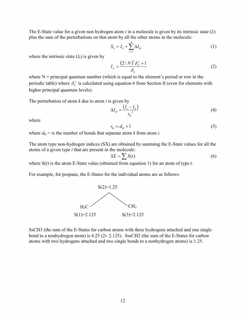
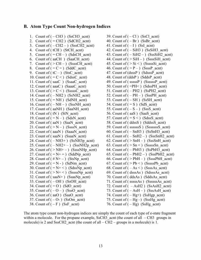
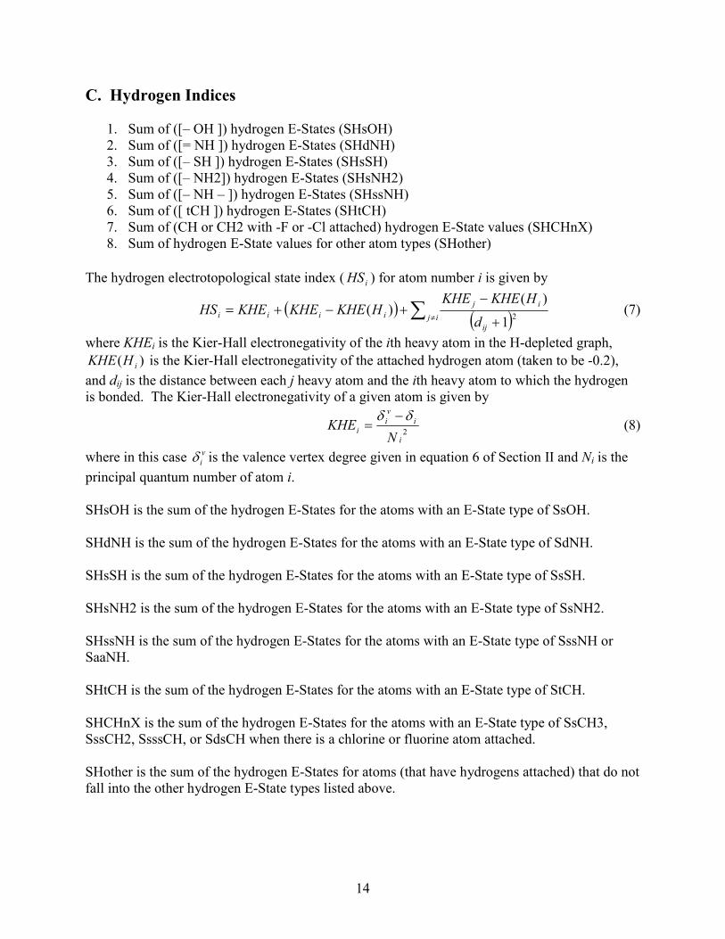
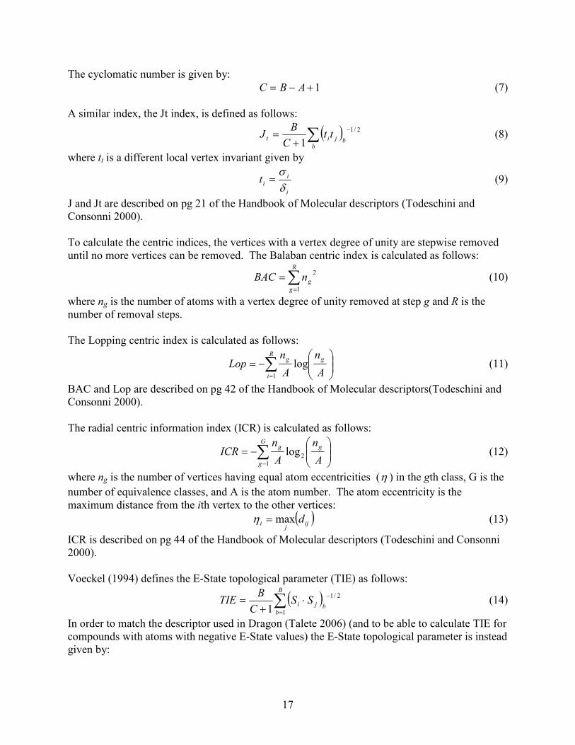
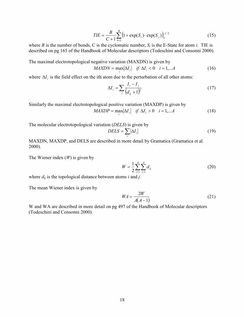
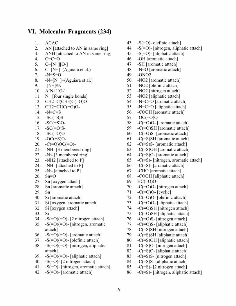
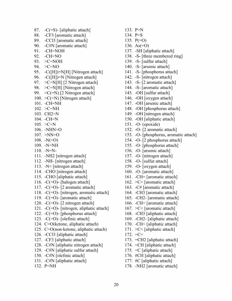
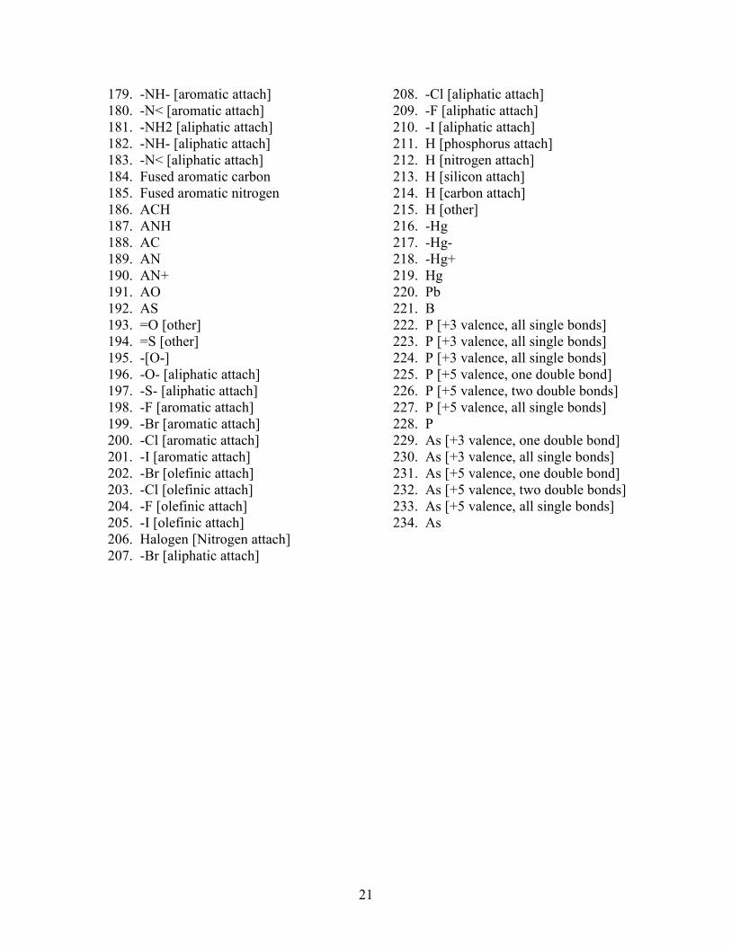
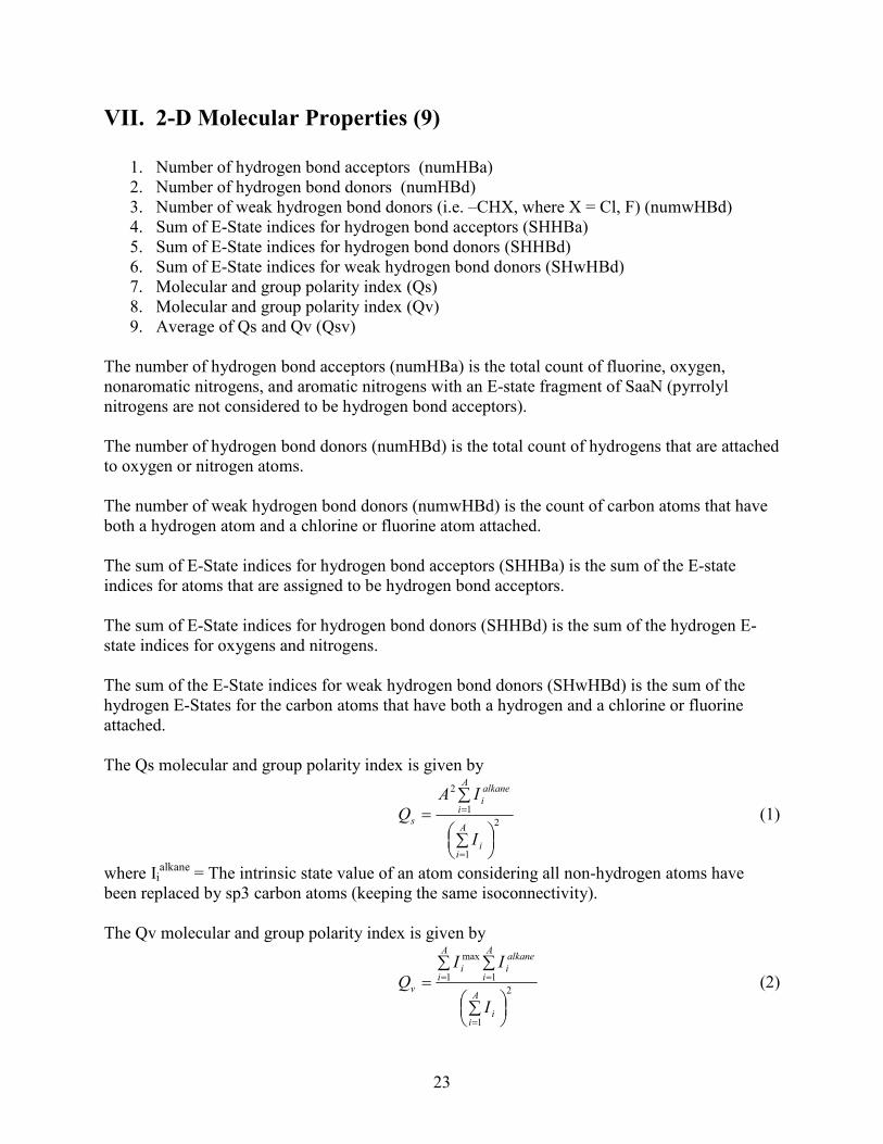
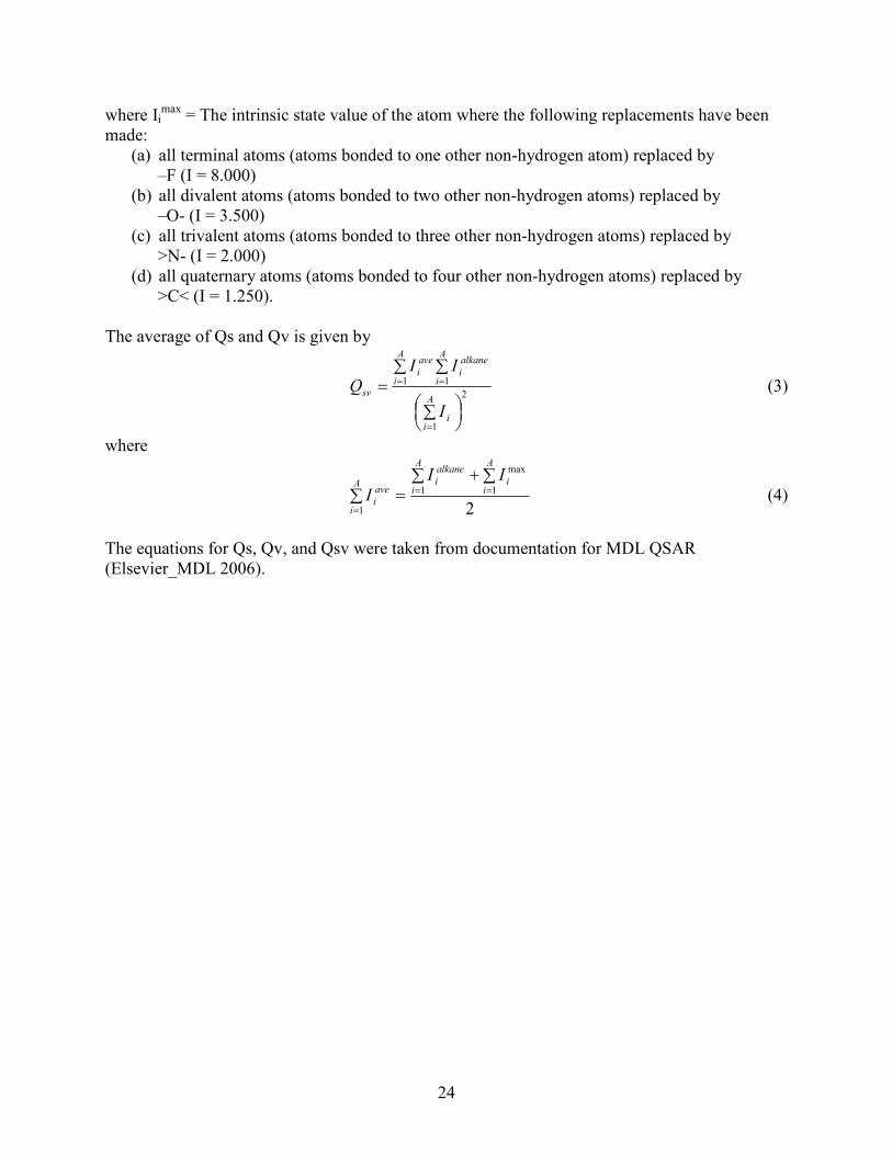
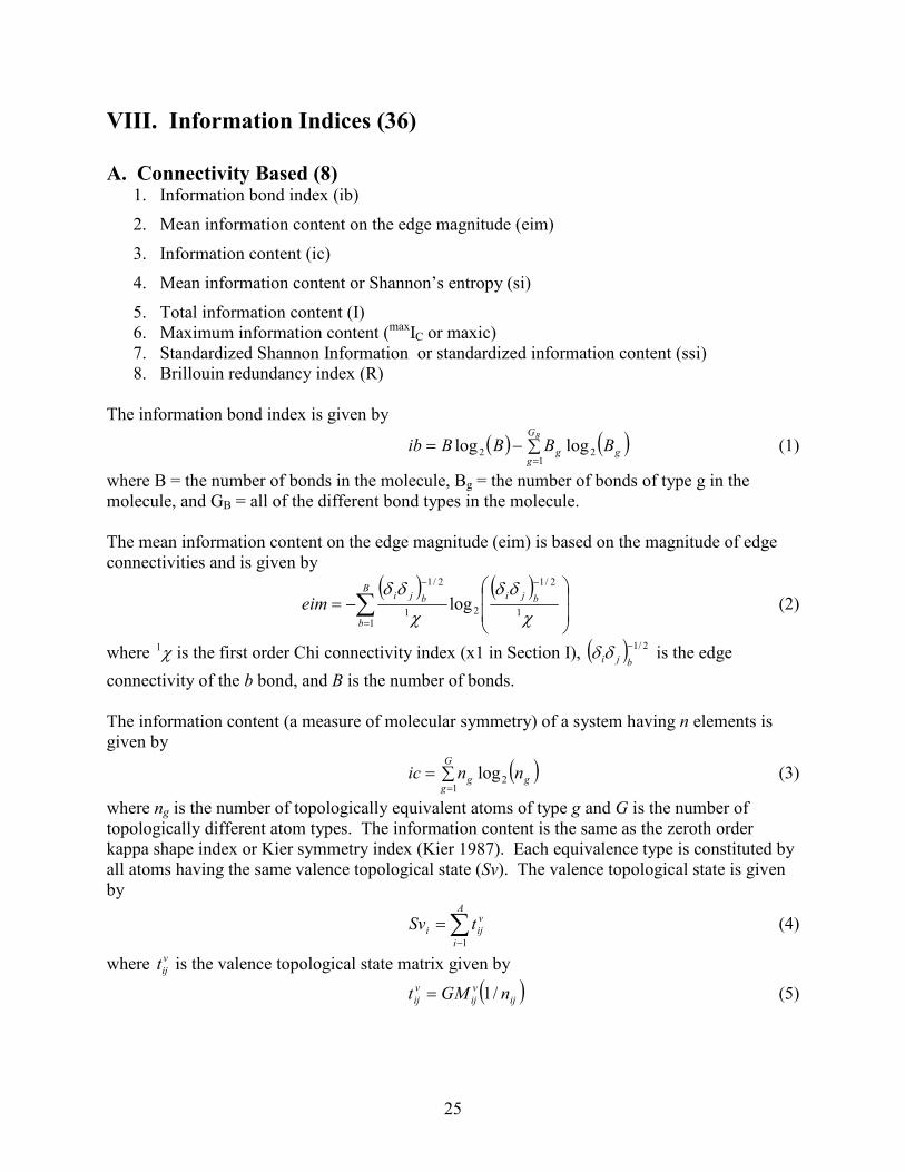
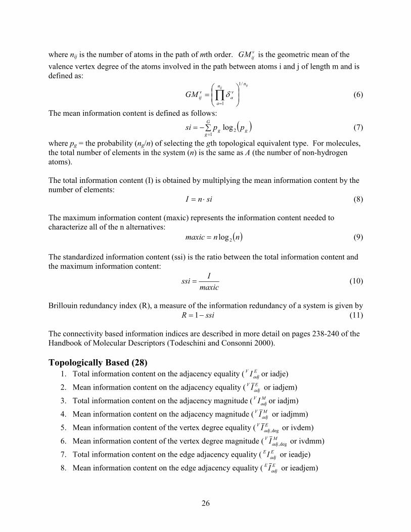
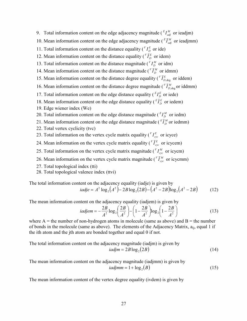
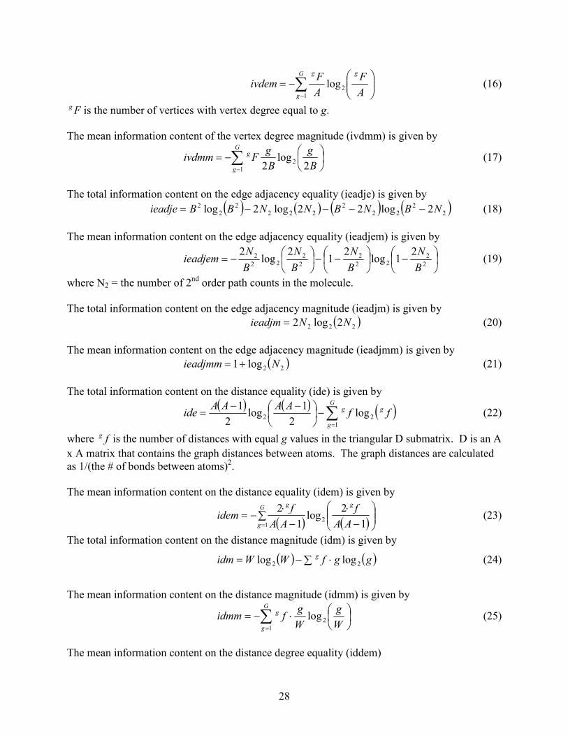
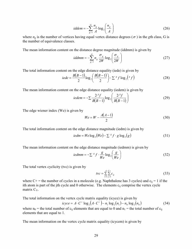
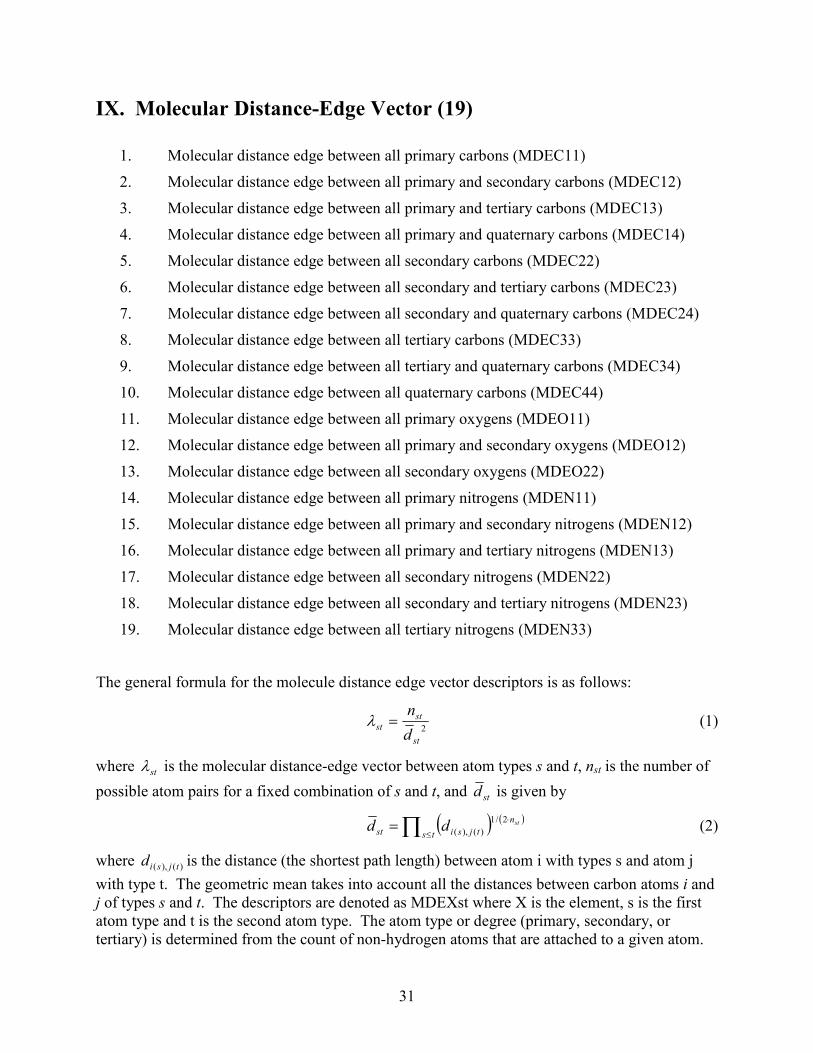
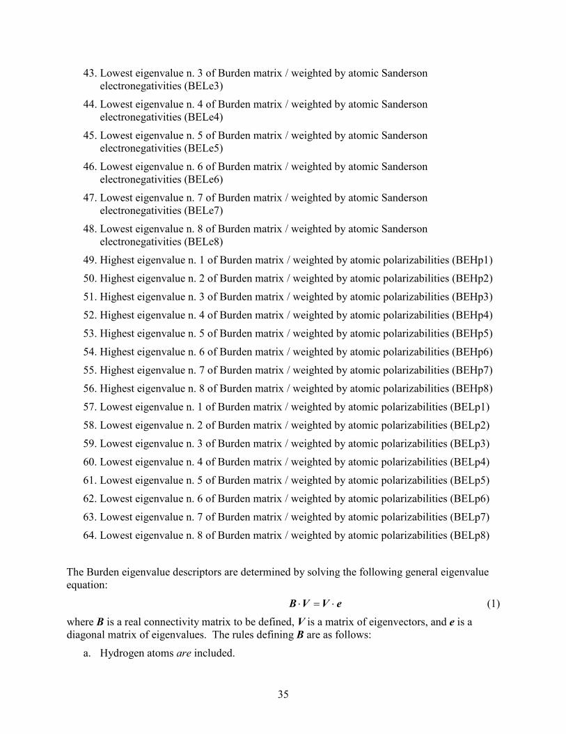
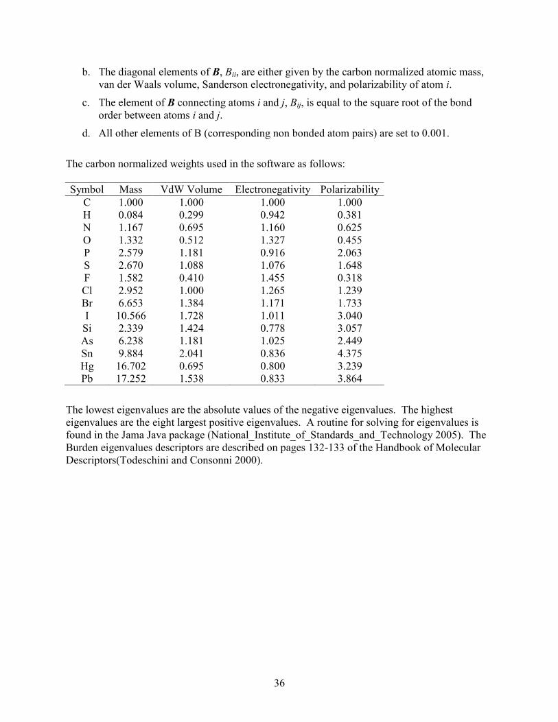
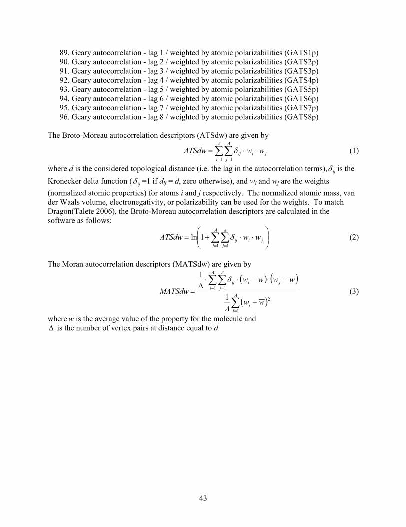
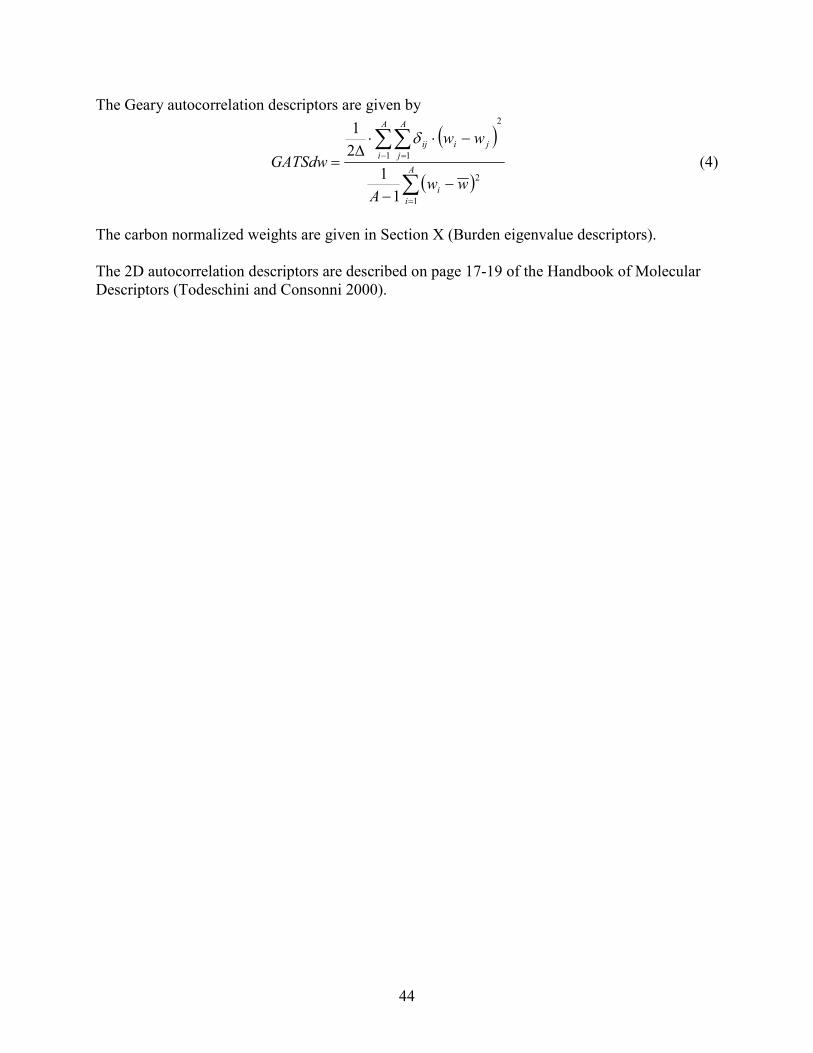
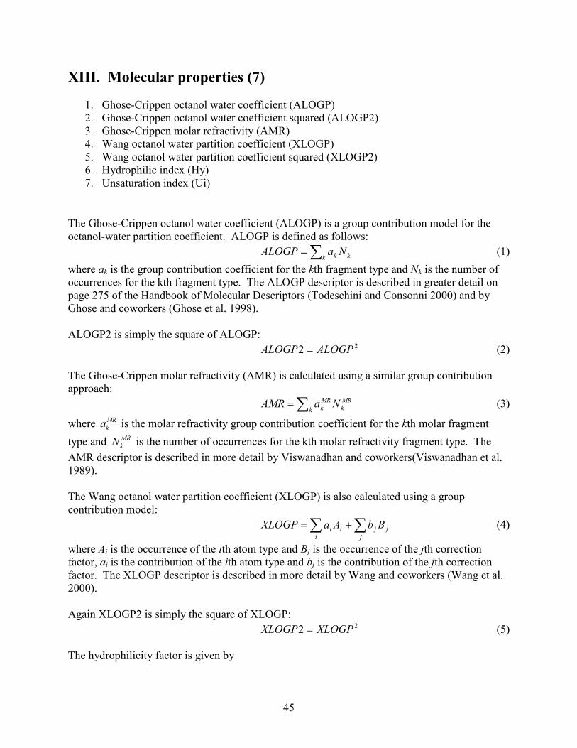
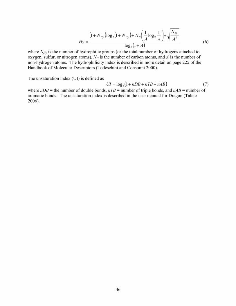