modelling realistic outcomes using integrated cost ... · this paper may not be reproduced or...

2017 AACE® INTERNATIONAL TECHNICAL PAPER

RISK-2510.1 Copyright © AACE® International.

This paper may not be reproduced or republished without expressed written consent from AACE® International

(RISK-2510)

Modelling realistic outcomes using Integrated Cost & Schedule Risk Analysis

Colin H Cropley

Abstract After several decades of development of project quantitative risk analysis for time and cost forecasting of project outcomes, achievement of consistently accurate results has remained elusive. Realistic time forecasts of projects have been found to be forecast well by sound Monte Carlo Method based SRA processes integrating schedule impact risk events. But realistic cost forecasting has proven more problematic. This paper demonstrates the capacity of Integrated Cost & Schedule Risk Analysis (IRA) to utilise parametric methods to represent and model systemic risks and to include decision-making during iterations to represent realistic treatment of project risks. But IRA can be extended to incorporate modelling of operation of the assets created by the project to produce probabilistic cashflows based on Capex and Opex uncertainties and risk events as well as revenue uncertainties and risk events, escalation and exchange rate uncertainties and risk events. In this way integrated modelling and scenario analyses can embrace the Total Cost Management framework envisaged by AACEI to support project FID.




Table of Contents Table of Contents List of Tables List of Figures List of Equations Introduction Acknowledgements What is Integrated Cost & Schedule Risk Analysis (IRA)? When is IRA most effective? Criticisms of CPM-Based Contingency modelling and responses Quantifying Contingencies fails to assess significant causes of failure of projects Extension of IRA Methodology to model operation of the assets from the project Example IRRA Model: The Generic Tollway – a Build, Own & Operate Public Private Partnership Project

(“GTP PPP”) Strengths and weaknesses of the IRA and IRRA methodologies How well does the IRA methodology address the criteria for quantifying project risk? Conclusion References List of Tables Table 1 – Base Tolls and Traffic Volume Growth Assumptions Table 2 – Inputs & Outputs of Hollmann Systemic Risk Cost Growth Table Table 3 – Inputs & Outputs of Hollmann Systemic Risk Schedule Slip Table Table 4 – Alignment of IRA to RP 40R-08 Principles List of Figures Figure 1 - IRA Methodology Flow Diagram Figure 2 - Generic Tollway Project Summary Schedule Figure 3 – Generic Tollway Asset Operations , Costs and Revenues Summary Schedule Figure 4 – Generic Tollway Extra Lanes Expansion Project and Operation Figure 5 – Sigmoid Curve for initial traffic growth Figure 6 – Possible Rail Line construction and operation from Year 11 Figure 7 – Extra Lanes Project construction and operation from Year 15 Figure 8 – Project specific risk events, treatments & mappings to PRA Schedule Figure 9 – Duration Histogram for design and construction of the GTP Figure 10 – Cost Histogram for design and construction of the GTP Figure 11 – GTP Probabilistic Cost Drivers Figure 12 – Cost Histogram of Year 20 Revenue reduction due to rail Figure 13 – Date Histogram of Extra Lanes first year operation (Optimistic scenario) Figure 14 – IRR Histogram of optimistic scenario Figure 15 – NPV Histogram of optimistic scenario Figure 16 – Date Histogram of Extra Lanes first year operation (Pessimistic scenario) Figure 17 – IRR Histogram of pessimistic scenario Figure 18 – Comparison of NPVs of Optimistic & Pessimistic Scenarios




Introduction A purpose of this paper is to describe the use of Integrated Cost & Schedule Risk Analysis (“IRA”) to model project time and cost outcomes realistically while meeting the requirements of the conference track on alternative methodologies for quantifying project risk. The methodology is explained, referencing industry practice as well as AACE RPs. The contexts in which the use of IRA methodology yields the greatest comparative advantages are described. A further aim of this paper is to describe an extension of the IRA methodology, to model the operation of the assets produced by the project, including risks to revenue and operations. The capacity of this Integrated Capital & Operating Costs, Schedule and Revenue Risk Analysis (“IRRA”) to model all kinds of risks to the project and resultant assets, in alignment with the Total Cost Management Framework, is illustrated by modelling of an example project and asset. The value of this is demonstrated by exploring scenarios involving threats and opportunities affecting the viability of the asset produced by the project. Also highlighted are the abilities of IRA and IRRA methodologies to incorporate intelligent treatment of risks within simulations and to apply systemic risk assessed by parametric methods. The paper concludes with an appraisal of the strengths and weaknesses of the IRA and IRRA methodologies and a tabulation of how well the IRA methodology addresses the principles of AACE RP 40R-08 Contingency Estimating – General Principles [1]. Acknowledgements This paper and the modelling on which it is based could not have been produced without the substantial contributions of the following colleagues of the author: • Voytek Kawecki, Managing Director, Javelin Associates Pty Ltd of Sydney Australia, who

generously developed the project plan for the Generic Tollway Project (GTP) • Matthew Dodds, Principal Consultant of Risk Integration Management Pty Ltd, who

refined the GTP schedule and wrote the macro that controls the timing of the Extra Lanes Project.

• Robert Flury, Principal Programmer of Risk Integration Management Pty Ltd, who enabled Quantitative Exclusion Analysis to be performed on Oracle® Primavera Risk Analysis® version 8.6 and ran it.

What is Integrated Cost & Schedule Risk Analysis (IRA)? The methodology advocated by this paper largely conforms to RP 57R-09, written by Dr David T Hulett [2]. A description of the methodology advocated follows, after the diagram representing the methodology sequence (Figure 1).




Figure 1 - IRA Methodology Flow Diagram

• A detailed or summarised schedule that covers the entire project scope in sufficient detail to represent the project complexity and strategy realistically becomes the basis for the analysis. It is ideally free of constraints and is fully linked such that all activities include at least one start predecessor and at least one finish successor. The activities in the schedule subject to duration uncertainty are assigned three-point distributions based on workshopping or by separate interviews with schedule Subject Matter Experts (SMEs) from the project team. Such ranging may also provide correlation models for groups of tasks. Alternatively or additionally, schedule risk factors may be identified and applied to applicable groups of tasks, which will automatically assign effective correlation.

• The project estimate or control budget is overlaid on the schedule with costs split accurately into time-dependent and time-independent portions. The detail in the estimate is required to match the detail in the schedule such that costs with different risk profiles are able to be linked to the corresponding groups of activities. The costs are structured so that they roll up in the way required for reporting. The Basis of Schedule and Basis of Estimate applicable to the respective elements must be aligned so that they represent matching assumptions. The cost items in the estimate subject to cost uncertainty are assigned three-point distributions based on workshopping or by separate interviews with cost SMEs from the project team. Such ranging may also provide correlation models for groups of costs. Alternatively or additionally, cost risk factors may be identified and applied to applicable groups of tasks, which will automatically assign effective cost correlation. Combined cost and schedule risk factors may also be defined and applied.

• If the schedule is describing a construction project, probabilistic weather calendars representative of the weather patterns in the construction location should be assigned to the applicable activities, representing the seasonal variation in weather and effects on available working time appropriate to construction tasks more and less vulnerable to




weather. Where resource costs continue independent of work being suspended due to weather, the costs must accrue without interruption by weather calendars. For this reason costs are loaded into the schedule using hammock activities not affected by the weather calendars but linked to the tasks that are affected.

• Project-specific risks in the project risk register are reviewed with the project team SMEs and those risks with significant cost and or time impacts are mapped to the applicable tasks in the schedule model. The risk cost and time impacts subject to uncertainty may also be assigned three-point distributions by the SMEs. Where required high exposure risks may be assigned risk treatments by the SMEs to reduce the risk exposure to acceptable levels. These may require significant treatment activities and costs to be effective and these must be included in the treated risk plan developed.

• The first risk to be assigned is the 100% probability systemic risk that the project delivery organisation and project team will perform less than optimally in delivering the project, based on previous project delivery performance, with significant cost and time impacts on the project. Where reliable records of such performance are not available, use may be made of John K Hollmann’s recently published book on Project Risk Quantification [3], assessing systemic risks using parametric methods as per Chapter 11 if the project is in the process industries, or Chapter 15 if in other industries. Hollmann has also published a spreadsheet parametric model for calculating systemic cost and schedule risks for varying input conditions that is available to purchasers of the book. Inputs for the parametric model require careful assessment by experienced risk analysts based on interviews with senior managers of the delivery organisation and project team and reviews of the project characteristics, aided by prior project records where available. The systemic risk schedule and cost impacts are applied separately as follows. The duration impact is applied across all project execution activities as a schedule risk factor. This will generate time-dependent cost uncertainty from the time-dependent costs spanning various parts of the execution schedule. The time-independent cost impact (determined from the overall split in the project estimate) is applied via a hammock activity in the cost structure spanning the entire project execution duration. The systemic time-independent cost risk should be correlated 100% with the systemic duration risk factor.

• The treated-risk loaded IRA model is created and validated before being subject to Monte Carlo simulation. The results are reviewed and must make sense before being communicated to the stakeholders for review. The results should include date and cost histograms and cruciality and cost sensitivity tornado diagrams to indicate what is driving the results. A review of the results with the project stakeholders may be followed by modifications to the model and another round of analysis, repeated until the results are acceptable to the stakeholders as realistic and making sense.

• The analysis may be completed by use of Quantitative Exclusion Analysis (QEA), whereby the highest drivers of risk by sensitivity diagrams are sequentially excluded from the IRA model, re-analysed and time and cost uncertainty differences quantified at agreed probability levels. This eliminates dependence on sensitivities which are




unreliable in the presence of correlation inputs. This allows optimisation of project risk by revealing the true highest drivers of cost and time outcomes. Further changes to the model may be focused on reducing those highest drivers by agreed changes to project execution strategy.

When is IRA most effective? The maximum value of the IRA methodology is achievable just before Financial Investment Decision when the most mature estimate and schedule prior to commitment should be available. The methodology works best with a sufficiently detailed and integrated schedule that describes the full scope in a way that represents the complexities of the project and particularly its interdependencies. Such detail is to be expected at the latter stages of a Bankable Feasibility Study (BFS) or a Front-End Engineering Design (FEED) phase. But effective use can also be made of IRA during the Select or Pre-Feasibility Study Phase when it can help differentiate between alternative strategies on the basis of comparative timing or NPV advantages. Also IRA is useful during project execution to review how well the project is progressing against its expected contingency drawdown forecasts. Whenever it is used, care must be taken in using the IRA methodology that the schedule, estimate and risk register are fully aligned with each other. Criticisms of CPM-Based Contingency modelling and responses Several criticisms are levelled at CPM-based quantitative risk analysis [3, pp136, 137]:

• The required schedule quality for effective CPM-based QRA is significantly higher than is produced in many projects. In the experience of the author’s team, one of the most time-consuming aspects of an IRA consulting engagement is reviewing the project schedule provided for analysis and ensuring that its quality is brought to an acceptable standard for the analysis. However, it is rare not to be able to achieve this with the cooperation of the client, as most planners want their schedule to be of an acceptable standard. The process also improves the understanding of planners of the reasons for and importance of the technical requirements for SRA schedule quality. A resource-loaded schedule is usually avoided because the detail is often unhelpful and where probabilistic weather calendars are involved, it is best to load the cost estimate separately from the schedule activities, as explained in describing the IRA methodology.

• Risk responses or treatments often require changes to the schedule to meet the changed circumstances, including attempting to preserve the project completion date. But modelling such logic changes in CPM-based models are viewed as difficult unless probabilistic branching is used and even then increased cost trade-off for reduced schedule slippage is deemed difficult to model. Again in the author’s team’s experience, workshop discussions of how to treat significant risks often may start with the assumption of a largely schedule slippage impact but subsequently agree on a largely




cost based consequence with the risk treatments involving additional expenditure to reduce or remove schedule impact. As will be seen later in this paper, the example project includes logic changes to the model during iterations that are driven by a macro.

• CPM-based risk analysis does not handle systemic risk well without special provision. This is accepted and this paper is partly intended to demonstrate how this can be done through the modified use of Hollmann’s Hybrid Approach for CPM-based Risk Modelling of Systemic Risk [3, Appendix A].

Quantifying Contingencies fails to assess significant causes of failure of projects One of the disadvantages of a focus only on quantifying project risk and thus contingency is that a surprisingly frequent cause of loss of viability of a project is not due to threats to the project but to the assets produced by the project. Many thousands of experienced project personnel are now out of work because demand for many commodities has fallen away, and with that fall in demand the prices of most minerals and metals, bringing to an end, from around 2013, the mining boom that started around 2003. The huge increase in production of unconventional oil & gas in America resulted in a halving in the prices of crude oil from 2014 and subsequently, the pricing of natural gas, especially liquefied natural gas, the contract pricing of which has been mostly linked to the price of crude oil. In addition, demand for fossil fuels is under threat from concern about global warming and advances in renewable energy technologies such as of solar photovoltaic cells, electric vehicles and battery storage. As a result of the precipitous fall in crude oil pricing, all oil & gas projects that were not committed beyond the point of no return were cancelled or deferred. That has caused the loss of hundreds of thousands of jobs worldwide as projects justified by crude oil pricing above $100/bbl became unviable at crude pricing below $50/bbl. Projected revenue from the assets produced by the project could no longer produce an adequate return on investment. In the infrastructure sector, there have been a number of tollways in several capital cities in Australia that have failed to achieve their forecast revenue because the traffic forecasts by consulting engineering companies were very optimistic compared with the actual traffic uptake. Where alternative routes were available, motorists have proven to be much more sensitive to toll pricing than the forecasts predicted. In the IT sector, there have been instances of projects delivering products that had been superseded by technology and no longer wanted. Examples include mainframe and mini-computers superseded by rising capabilities and falling prices of personal computers and the Nokia and BlackBerry mobile phones, overtaken by the iPhone and other smartphones. There is a clear need for the ability to model not just the project but the operation of the produced assets of the project, so that the resilience of the project plus assets can be subjected to threats to asset operating revenues and operating costs as well as to threats to the project itself.




Extension of IRA Methodology to model operation of the assets from the project IRRA Methodology Basis The IRA methodology, being built on CPM integration of time and cost, can produce probabilistic cost flows. If the methodology is extended beyond commissioning and startup of the assets produced by the project to incorporate operation of the assets, opportunities open up to examine the overall viability of the investment proposal. The operating costs and generation of revenues produced by those assets, together with the uncertainties and risks attributable to those operations, costs and revenues, allow probabilistic cashflows to be generated that encompass the complete project and assets life-cycle. That allows probabilistic Net Present Values (NPVs) and Probabilistic Internal Rates of Return (IRRs) to be derived. And if discount rates for the time-dependent value of money, together with other parameters such as the interest rate for borrowed project finance funds are added in, useful projections for the financial viability of the investment proposal can be evaluated. Scenarios can then be assessed to determine the resilience of the investment in the face of various challenges and threat combinations. The above is the basis for the extension to the IRA methodology to perform Integrated Capital and Operating Costs, Schedule and Revenue Risk Analysis (IRRA). Such analysis is limited only by the ingenuity of the risk analyst, supported by economic analysts and the limitations of the CPM-based Monte Carlo Simulation tool being used. Functionality needed for effective IRRA modelling The following functionality is considered necessary for IRRA modelling to be performed: • Ability to combine Cost Risk Analysis with Schedule Risk Analysis in the one

simultaneous Monte Carlo simulation; • Ability to generate probabilistic cashflows combining expenditures and revenues; • Ability to apply risk factors with time and/or cost impacts and to correlate those risk

factors to each other; • Ability to define risk events with definable cost and schedule impacts, treat them with

multiple treatments with definable duration and cost range tasks and map them to a cost-loaded CPM-based schedule to create single or multiple risk-tasks and treatment tasks in a treated risk plan, with appropriate flexibility over correlation of existence of multiple risk-tasks;

• Ability to apply positive and negative correlation to duration ranging, cost ranging and existence of risks;

• Ability to apply macros to the model to enable logic changes to occur within simulation iterations;

• Ability to apply selectable Discount Factors to the cash flow to represent the changing value of money over time;

• Ability to apply variable interest rates to the cost of project finance. The author’s team has used Oracle® Primavera Risk Analysis® (PRA) to produce IRRA models to demonstrate the value of such modelling. Other tools are being provided with capabilities that enable them to do such modelling also, including BAH’s Polaris® and Safran Risk®. But so far,




not enough of the above functionality features are yet available in other products, to the knowledge of the author’s team. Example IRRA Model: The Generic Tollway – a Build, Own & Operate Public Private

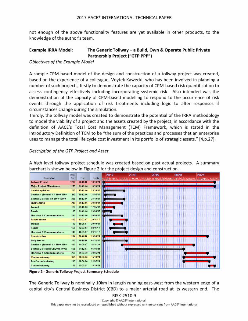
Partnership Project (“GTP PPP”) Objectives of the Example Model A sample CPM-based model of the design and construction of a tollway project was created, based on the experience of a colleague, Voytek Kawecki, who has been involved in planning a number of such projects, firstly to demonstrate the capacity of CPM-based risk quantification to assess contingency effectively including incorporating systemic risk. Also intended was the demonstration of the capacity of CPM-based modelling to respond to the occurrence of risk events through the application of risk treatments including logic to alter responses if circumstances change during the simulation. Thirdly, the tollway model was created to demonstrate the potential of the IRRA methodology to model the viability of a project and the assets created by the project, in accordance with the definition of AACE’s Total Cost Management (TCM) Framework, which is stated in the Introductory Definition of TCM to be “the sum of the practices and processes that an enterprise uses to manage the total life cycle cost investment in its portfolio of strategic assets.” [4,p.27]. Description of the GTP Project and Asset A high level tollway project schedule was created based on past actual projects. A summary barchart is shown below in Figure 2 for the project design and construction.

Figure 2 - Generic Tollway Project Summary Schedule The Generic Tollway is nominally 10km in length running east-west from the western edge of a capital city’s Central Business District (CBD) to a major arterial road at its western end. The




westernmost 2km of the tollway consists of two tunnels: one for the three inbound lanes and one for the three outbound lanes. The other 8km of the tollway runs east from the tunnels to the western edge of the CBD, crossing over two major roads. The schedule was extended past commencement of tolling to cover 25 years of operation. Allowance was made for growth in use of the tollway (as described under Operations below) such that an extra lane in addition to the three lanes each way could be justified to cope with the extra traffic and to ease congestion. The extra lanes constitute a treatment of a threat of increasing congestion and travel times, albeit an expensive and elaborate treatment. The decision on whether to apply for approval to install extra lanes and proceed with the expansion project depends on the volume of traffic per day and toll revenue to justify the further investment. The timing of the Extra Lanes Project (ELP) could vary widely, depending on the growth rate of traffic and revenue. It could be justified after just five years of operation or may never be justifiable within the twenty-five years of modelled operations, due to insufficient growth. Complicating the growth potential of the Generic Tollway is the threat that the State Government may decide to install a commuter railway line parallel to the Tollway, which would adversely affect traffic volumes and revenue of the Tollway. The negative effect is expected to be such that the ELP is not expected to be justifiable in the twenty-five years of operation modelled. The first nine of those 25 years of operation is shown summarised below in Figure 3, including the possible extra lanes expansion.

Figure 3 – Generic Tollway Asset Operations , Costs and Revenues Summary Schedule




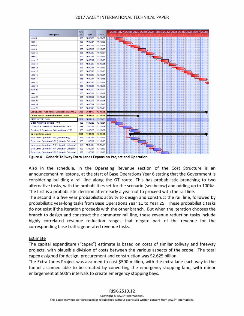
How the GTP and Tollway Operation were modelled Schedule The schedule starts from commitment to proceed with the tollway. The construction project ends with a milestone marking commencement of tolling. The schedule is structured so that the design, procurement and construction of the tollway comprise a section, the tollway asset operation is another and the project to construct and operate extra lanes is a third section. This enables separated analysis and reporting. The capital and operating costs and revenue are separated from the project and extra lanes construction and operations activities. This enables the costs to be structured optimally for reporting and analysis purposes and, as described earlier, enables costs to continue accruing even when construction is interrupted by adverse weather. Risks (placeholder tasks) and treatments make up a further section of the schedule. The risk-tasks are embedded with their parent tasks. Statistically, the schedule consists of 429 activities, of which 194 are normal (non-zero duration, take part in CPM calculations), 108 are summaries (heading tasks), 28 are milestones and 99 are hammocks (for capturing the project and operating costs and revenue). Three calendars are used: Standard (5d/w), 6 Day and 7 Day. The deterministic critical path for the construction project goes through tunnel design and tunnelling equipment procurement to tunnel construction and completion, power, lighting and traffic management and tolling systems installation and commissioning. Operations consist of a series of one-year long tasks (not subject to duration uncertainty) from Year 1 Operation to Year 25 Operation. Extra Lanes Project (ELP) Also included in the Operations phase of the schedule is an offset task with probabilistic successors defining design and approvals, construction and commissioning of an extra lane inbound and outbound over three years, followed by 10 years of probabilistic operation of the extra lanes, as shown below in Figure 4. These construct, commission and operations tasks are linked to hammock tasks in the cost structure section of the schedule. The existence and timing of these tasks are controlled by a VBA macro which is described below under Operations.




Figure 4 – Generic Tollway Extra Lanes Expansion Project and Operation Also in the schedule, in the Operating Revenue section of the Cost Structure is an announcement milestone, at the start of Base Operations Year 6 stating that the Government is considering building a rail line along the GT route. This has probabilistic branching to two alternative tasks, with the probabilities set for the scenario (see below) and adding up to 100%: The first is a probabilistic decision after nearly a year not to proceed with the rail line. The second is a five year probabilistic activity to design and construct the rail line, followed by probabilistic year-long tasks from Base Operations Year 11 to Year 25. These probabilistic tasks do not exist if the iteration proceeds with the other branch. But when the iteration chooses the branch to design and construct the commuter rail line, these revenue reduction tasks include highly correlated revenue reduction ranges that negate part of the revenue for the corresponding base traffic generated revenue tasks. Estimate The capital expenditure (“capex”) estimate is based on costs of similar tollway and freeway projects, with plausible division of costs between the various aspects of the scope. The total capex assigned for design, procurement and construction was $2.625 billion. The Extra Lanes Project was assumed to cost $500 million, with the extra lane each way in the tunnel assumed able to be created by converting the emergency stopping lane, with minor enlargement at 500m intervals to create emergency stopping bays.




The base traffic revenue figures were built up assuming tolls for several different classes of vehicle, with the following growth assumptions, based on the Annual Volume = Avg. Daily Rate x 350; allowable price growth of tolls/year of CPI (assumed 2.5% pa). Assumed growth per year in traffic volumes of g% was 1%.

Vehicle Class Toll/avg. trip Toll Incr./Y Ramp-up assumptions Cars/Light Vehicles $2.50 CPI To 150,000/d in 5y, then grow at g% pa Medium trucks $5.00 CPI To 30,000/d in 3y, then grow at g% pa Semi-trailers $10.00 CPI To 15,000/d in 3y, then grow at g% pa B-Doubles & Triples $25.00 CPI To 5,000/d in 3y, then grow at g% pa

Table 1 – Base Tolls and Traffic Volume Growth Assumptions The Ramp-up figures were derived from use of a “Sigmoid Curve” using the following formula and graph (Figure 5):

Figure 5 – Sigmoid Curve for initial traffic growth The curve was adjustable by multiplying the y function value by the ramp-up number and substituting year number for the t-values. Ranging around the Most Likely base traffic figures was wide – Min: 70%, Max: 140%, of ML. The base annual operating expenditure (“opex”) was taken as a base fixed cost ($500,000) plus a percentage of annual revenue (2.5%). The Extra Lanes traffic, revenue and opex ramp-ups and growth were based on appropriate fractions of the base year revenues during ramp-up Extra Lane Operation Years 1(ELO Y1), ELO Y2, ELO Y3, then successive years ELO Y4-10. ELO opex for the corresponding years was based on appropriate fractions of Base Years Opex. The threat of Rail Line reducing Car traffic was assumed to start suppressing revenue figures from Base Operation Year 11, by adding negative revenue based on the Sigmoid curve ramping to -50,000 cars per day over four years (BO Y11-14), then the negative growth to increase by 3.0% per annum from Y15 to Y25.




Operations The decisions on whether and if so, when, to proceed with the ELP and how the decision of the government to proceed with the railway line or not affects the ELP are incorporated in a VBA macro embedded in the IRRA model written by the author’s colleague Matthew Dodds. The government decision on whether to build the railway line is incorporated in the IRRA model as a probabilistic branch with selectable probability. The way the VBA macro works within the simulations is as follows: A user-selectable fixed threshold annual revenue figure is input at the top of the macro before the simulation to represent the amount of revenue in any one year sufficient to trigger the ELP permit application, construction and operation. A lower figure will enable the ELP to initiate earlier and begin generating increased revenue earlier. The macro next checks if, in this iteration, the railway is to be built and operated or not (it does this by checking if the remaining duration of one of the early rail line operating activities is >0, which can only happen if the rail line is to be built). If the rail line is to be built in this iteration, the macro will terminate and no ELP project will occur. If no rail project is to be built in this iteration, the macro will check each year of assigned revenue from Year 01 to Year 16 to see if the threshold revenue amount has been met or exceeded in any of those years. If it has, that year becomes the start of the ELP: the three years of permits/design and construction and the subsequent 10 years of operation. If the threshold revenue figure is not reached in any of the years up to Year 16, the ELP is not initiated in that iteration. So there are three possible operating conditions simulated in Generic Tollway IRRA modelling:

1. The rail line is installed and operated from Base Traffic Operation Year 11 and no extra traffic lanes are installed.

2. The rail line is not installed and the Extra Lanes Project (ELP) is initiated from the first year in which the revenue threshold is exceeded. This could be as early as Revenue Year 01 and as late as Revenue Year 16, depending on input settings.

3. Neither the rail line nor the extra lanes are installed because the revenue earned in each year falls short of the selected threshold.

The following screen dumps show: • The rail line being built and operated from Year 11 (Figure 6) and • The Extra Lanes Project being triggered by in Year 13 and operated from Year 15 (Figure 7)




Figure 6 – Possible Rail Line construction and operation from Year 11 The following screen dump shows the ELP being triggered and operated from Year 15:

Figure 7 – Extra Lanes Project construction and operation from Year 15 Risk Three kinds of risk were incorporated in the GTP IRRA model:

1. Systemic Risk that the project delivery organisation and team may perform less than optimally in delivering the project;

2. Estimating uncertainty in time and cost such that ranges are assigned to line items and task durations rather than single values;

3. Project specific risk events that have been identified by the project team as applying to this project and the operation of this asset produced by the project.

Taking each of these in turn:




Systemic risk has been modelled based on the parametric method advocated by John Hollmann [3, Chs 11 & 15 & App A] where documented performance of the project delivery organisation in previous projects is not available. The method described in Ch11 is for the process industries, but is adapted for the transport sector in Ch15. However, the author believes that systemic risk using the Hollmann method does not replace underlying estimate and duration uncertainty, which are set through ranging involving Subject Matter Experts (SMEs). The systemic risk added covers organisational flaws and less than optimal project delivery performance. A set of values has been substituted into Hollmann’s Spreadsheet Template (made available with his book), based on the example given in Chapter 15 for Transportation. But the implementation of the systemic risk in IRA is through application of a duration risk factor (to generate time-dependent costs) and a cost hammock (for ranged time-independent costs) across GTP design and construction, rather than through a single systemic risk activity at the end of the GTP construction phase as proposed by Hollmann [3, App A]. This is to distribute the cost and schedule impacts through the construction phase to provide a consistent basis for probabilistic cashflow and probabilistic IRRs and NPVs as part of the IRRA methodology. If the purpose were solely to produce probabilistic time and cost forecasts for completion of the execution of the project, the Hollmann approach of adding a single systemic risk activity just prior to the project end milestone would be quite acceptable and more straightforward to implement in an IRA model. However, the Hollmann method does not work if the parametric method requires application of a negative schedule slippage percentage at the P10 level, as this modelling does. Hollmann’s Hybrid method [3, App A] proposes a systemic risk task of duration equal to the P50 percentage of the project deterministic duration generated from his parametric model, with ranging corresponding to the P10, P50 and P90 percentages of the project deterministic duration. But in the case below, the P10 duration of the systemic risk task would be negative, which is not possible. The problem is overcome using a duration risk factor across the project as adopted here. The cost range to be loaded on the systemic risk task also includes a negative P10 value, but that is permissible for resources. The following assumptions were made to provide inputs to the Systemic Risk Cost Growth table in Hollmann’s spreadsheet (see Table 2 below). Note that in a real project, these inputs can only be made after interviews with senior delivery organisation management, workshopping and careful consideration of the quality of the inputs received for the risk analysis. The project was assumed to be conducted by an experienced tollway project delivery organisation with well-developed definition of scope, planning and engineering, giving an overall scope definition rating of 3, complying with definition phase requirements. Given that it is tollway with proven tolling system, there is 0% new technology and process severity is inapplicable. Complexity is moderate given the tunnelling and tolling systems plus land acquisition and need for minimal disruption to city traffic during construction. The team development is rated as fair, but the project control and estimate basis are good. There is a small percentage of equipment (the tolling system) required to be installed. 40% of the project by value is to be performed on a fixed price basis. Bias of the estimate is assessed as typical.




The spreadsheet template was filled in as follows for Cost, giving the indicated mean contingency and the forecast three point distribution values for systemic risk time-independent cost. The proportion of total cost of the project represented by time-independent cost is required under the IRA methodology and can be obtained from the estimate. Excluding weather effects, the time-independent cost proportion of the project capex is 35.4%.

Table 2 – Inputs & Outputs of Hollmann Systemic Risk Cost Growth Table The following assumptions were made to provide inputs to the Systemic Risk Schedule Slip table in Hollmann’s spreadsheet (see Table 3 below). The same comments apply as for the Cost Growth inputs regarding the need for interviews, workshops and consideration of the quality of the inputs. The quality of the schedule for the Generic Tollway Project was assumed to be only fair, even though the project controls were considered to be good, which is not an unusual situation. As for the estimate, the schedule bias was assumed to be typical. These schedule assumptions led to the following schedule mean impact and the resultant schedule three point distribution using the Hollman Spreadsheet template.

COST GROWTH RISK DRIVER ENTER PARAMETER (a) COEFFICIENT (b) a*b CONSTANT -30.5 SCOPE 3 PLANNING 3 ENGINEERING 3 SCOPE DEFINITION 3.0 9.8 29.4 NEW TECHNOLOGY 0% 0.12 0.0 PROCESS SEVERITY 0 1 0.0 COMPLEXITY 3 1.2 3.6

SUBTOTAL BASE (prior to adjustments) 2.5

ADJUSTMENTS Complex Exec Strategy? > No Team Development Fair 0 Project Control Good -1 Estimate Basis Good -1 Equipment 5% 4 Fixed Price 40% -3 TOTAL BASE (prior to bias adjustment; rounded to whole number) 2 Bias Typical 0

SYSTEMIC COST CONTINGENCY (at shown chance of underrun) MEAN 2% 10% -5% 50% 1% 90% 9%




Table 3 – Inputs & Outputs of Hollmann Systemic Risk Schedule Slip Table From the project estimate, excluding growth due to weather, the time-dependent costs represent 64.6% of total costs. So the time-dependent cost systemic risk is ranged around this proportion of the mean cost of the Capex of the project (including growth due to weather). The systemic time-independent cost risk was correlated 100% with the systemic duration risk factor using the correlation interface provided in PRA. It is also worth noting that under these assumptions, systemic schedule risk is substantially greater than cost risk, especially at the pessimistic end. This mirrors experience in Australia with Public Private Partnerships (PPPs) for major tollway projects for the States, who are the ultimate owners of such projects. There have been significant schedule overruns on such projects, especially where tunnelling has been involved. There have been PPPs where the consortia executing the work have suffered serious financial losses on such projects because they carry the fixed price risk. Estimating uncertainty in time and cost ranges assigned to task durations and cost estimate line items have been assigned using techniques applied in IRA consulting engagements over the past eight years. The element missing in this demonstration model is a very important part – engagement with the project stakeholders and subject matter experts by interviews or workshops to collect the uncertainty ranges for groups of activities and cost estimate line items. The duration uncertainty applied to the activities in this model was generated using judgment and coding of groups of tasks to assign both ranges and correlation. Cost ranging was applied using a spreadsheet tool developed by the author’s colleague Matthew Dodds to support and facilitate the IRA methodology. Correlation was applied to groups of resources using a cost correlation tool written by Matthew Dodds in VBA in PRA 8.6.

EXECUTION SCHEDULE DURATION SLIP RISK DRIVER ENTER PARAMETER (a) COEFFICIENT (b) a*b CONSTANT -23.5 SCOPE DEFINITION 3.0 9.6 28.8

NEW TECHNOLOGY 0% 0.1 0

PROCESS SEVERITY 0 0.5 0

COMPLEXITY 3 0.5 1.5

SUBTOTAL BASE (prior to adjustments) 6.8

ADJUSTMENTS Schedule Basis Fair 0 TOTAL BASE (prior to bias adjustment; rounded to whole number) 7 Bias Typical 0

SYSTEMIC EXECUTION SCHEDULE DURATION CONTINGENCY MEAN 7% 10% -3% 50% 6%

80% < enter funding p-level (increments of 10%) 12%

90% 16%




Project specific risk events were created in a risk management database developed by the author’s colleague Robert Flury to manage risks through their lifecycle and map them to PRA schedules (see Figure 8 below). These risks included the systemic risk to delivery of the project, the opportunity presented by increasing traffic to construct extra lanes and the threat that the Government may build an adjacent rail line that reduces usage of the tollway. This was to enable these risks to be managed. However they were made inactive because they have been handled as described above. The active risks and treatments and the task IDs to which they were mapped are shown on the following page. The probabilistic financial and durational impacts are totalled at the bottom of the table. These totals indicate the potential aggregate magnitude of the active treated risks upon a Monte Carlo simulation. A comparison of these probabilistic totals with the total cost and duration of the Generic Tollway Project reveals that these project specific risks are not a significant threat to the project outcome. This is a misleading indication of the significance of risks on this project because risks with big probabilistic impacts on the project are operational – threat of an adjacent commuter rail line and the opportunity of increased usage requiring extra traffic lanes – and have been modelled in a different way, as described.

Figure 8 – Project specific risk events, treatments & mappings to PRA Schedule




Results obtained and Scenarios modelled The GTP Project and Asset Operation IRRA Model is a mixture of construction and operation, of capex, opex and revenue. The scenarios used to illustrate the potential of the methodology have focused on aspects not usually encountered in conventional contingency assessment. In this tollway model, two scenarios are presented to demonstrate how such a model may be used. The numbers and results are less important than the demonstration of the approach. Results for Design and Construction of Tollway Project The planned duration of the design and construct project is affected by three elements that combined to make the deterministic project duration unachievable: • A neutral or slightly pessimistic bias of the ranging of the project execution activities; • The probabilistic addition of weather pessimism not included in the deterministic dates; • The addition of the emphatically pessimistic systemic duration risk factor to all project

execution activities (97% Optimistic/106% Most Likely/116% Pessimistic) This shows in the deterministic duration probability of the following project duration histogram (see Figure 9 below), which is <1%:

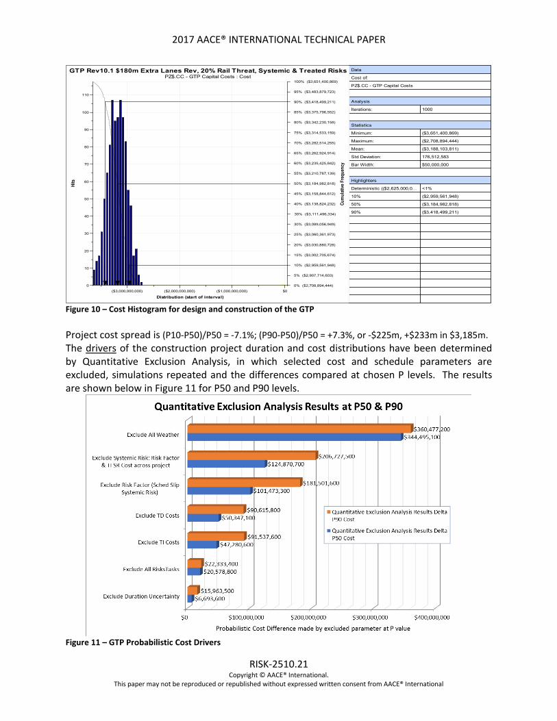
Figure 9 – Duration Histogram for design and construction of the GTP The spread of duration around the P50 is (P10-P50)/P50= -6.0%; (P90-P50)/P50 =+6.3%, which is quite credible. It represents just under -3 months, + just over 3 months, in about 48 months. The deterministic project capex of $2,625 million is also at an unachievably low probability (<1%) for similar reasons, with a P50 cost of $3,185 million (see Figure 10 below). Note that in a model including costs and revenue, costs are negative and PRA always includes $0 in the range of negative cost histograms:

Data

Duration of:

PC - Tollway Project

Analysis

Iterations: 1000

Statistics

Minimum: 1287

Maximum: 1631

Mean: 1457

Std Deviation: 67.03

Bar Width: week

Highlighters

Deterministic (1274) <1%

10% 1369

50% 1456

90% 1548

1300 1400 1500 1600

Distribution (start of interval)

0.0

5.0

10.0

15.0

20.0

25.0

30.0

35.0

40.0

45.0

50.0

55.0

Hits

0% 1287

5% 1351

10% 1369

15% 1384

20% 1395

25% 1405

30% 1415

35% 1424

40% 1439

45% 1449

50% 1456

55% 1465

60% 1474

65% 1484

70% 1494

75% 1504

80% 1517

85% 1529

90% 1548

95% 1569

100% 1631

Cum

ulat

ive

Freq

uenc

y

GTP Rev10.1 $180m Extra Lanes Rev, 20% Rail Threat, Systemic & Treated RisksPC - Tollway Project : Duration




Figure 10 – Cost Histogram for design and construction of the GTP Project cost spread is (P10-P50)/P50 = -7.1%; (P90-P50)/P50 = +7.3%, or -$225m, +$233m in $3,185m. The drivers of the construction project duration and cost distributions have been determined by Quantitative Exclusion Analysis, in which selected cost and schedule parameters are excluded, simulations repeated and the differences compared at chosen P levels. The results are shown below in Figure 11 for P50 and P90 levels.

Figure 11 – GTP Probabilistic Cost Drivers

Data

Cost of:

PZ$.CC - GTP Capital Costs

Analysis

Iterations: 1000

Statistics

Minimum: ($3,651,400,869)

Maximum: ($2,708,894,444)

Mean: ($3,188,103,811)

Std Deviation: 176,512,583

Bar Width: $50,000,000

Highlighters

Deterministic (($2,625,000,0... <1%

10% ($2,959,561,948)

50% ($3,184,982,818)

90% ($3,418,499,211)

($3,000,000,000) ($2,000,000,000) ($1,000,000,000) $0


0

10

20

30

40

50

60

70

80

90

100

110

Hits

0% ($2,708,894,444)

5% ($2,907,714,603)

10% ($2,959,561,948)

15% ($3,002,705,674)

20% ($3,030,880,728)

25% ($3,060,361,973)

30% ($3,089,056,949)

35% ($3,111,496,334)

40% ($3,138,824,232)

45% ($3,158,844,612)

50% ($3,184,982,818)

55% ($3,210,787,139)

60% ($3,235,425,842)

65% ($3,262,924,914)

70% ($3,282,514,255)

75% ($3,314,533,159)

80% ($3,342,230,158)

85% ($3,375,796,552)

90% ($3,418,499,211)

95% ($3,483,879,723)

100% ($3,651,400,869)

Cum

ulati

ve F

requ

ency

GTP Rev10.1 $180m Extra Lanes Rev, 20% Rail Threat, Systemic & Treated RisksPZ$.CC - GTP Capital Costs : Cost




Scenario 1: Low threshold revenue to add extra lanes, low probability of Rail Link being built An annual revenue threshold of $180 million was input to the macro to trigger earlier decisions to add extra lanes to the tollway. Also, a probability of 20% was placed on the likelihood that the government would build an adjacent commuter rail line. The following charts show how this affects the model. Figure 12 shows that Year 20 projected reduction of tollway revenue from the rail line in the 20% of iterations it occurs, of $10m/$20m/$30m.

Figure 12 – Cost Histogram of Year 20 Revenue reduction due to rail This reduction is only 4.1% of the P90 of Year 20 base revenue, of $471.1m. The probabilistic start date distribution for Year 1 for Extra Lanes Operation (ELO Y1) shows in Figure 13 that the start year always occurs in 2027 (Base Operation Year 6).

Figure 13 – Date Histogram of Extra Lanes first year operation (Optimistic scenario)

($30,000,000) ($20,000,000) ($10,000,000) $0


0

100

200

300

400

500

600

700

800

Hits

0% $0

5% $0

10% $0

15% $0

20% $0

25% $0

30% $0

35% $0

40% $0

45% $0

50% $0

55% $0

60% $0

65% $0

70% $0

75% $0

80% ($8,507,081)

85% ($15,749,259)

90% ($19,470,004)

95% ($23,174,963)

100% ($31,050,677)

Cum

ulat

ive

Freq

uenc

y

GTP Rev10.1 $180m Extra Lanes Rev, 20% Rail Threat, Systemic & Treated RisksPP.R.01.200 - Year 20 Revenue reduction by rail line : Cost

29/01/17 22/07/22


0

50

100

150

200

250

300

350

400

Hits

0% 01/12/16

5% 01/12/16

10% 01/12/16

15% 01/12/16

20% 01/12/16

25% 17/01/27

30% 31/01/27

35% 15/02/27

40% 26/02/27

45% 05/03/27

50% 14/03/27

55% 22/03/27

60% 01/04/27

65% 07/04/27

70% 16/04/27

75% 25/04/27

80% 03/05/27

85% 12/05/27

90% 27/05/27

95% 14/06/27

100% 22/08/27

Cum

ulat

ive

Freq

uenc

yGTP Rev10.1 $180m Extra Lanes Rev, 20% Rail Threat, Systemic & Treated Risks

XLANE.040 - Extra Lanes Operation - YR1 (Inbound Only) : Start Date




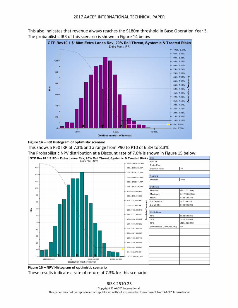
This also indicates that revenue always reaches the $180m threshold in Base Operation Year 3. The probabilistic IRR of this scenario is shown in Figure 14 below:

Figure 14 – IRR Histogram of optimistic scenario This shows a P50 IRR of 7.3% and a range from P90 to P10 of 6.3% to 8.3% The Probabilistic NPV distribution at a Discount rate of 7.0% is shown in Figure 15 below:

Figure 15 – NPV Histogram of optimistic scenario These results indicate a rate of return of 7.3% for this scenario

6.00% 8.00% 10.00%


0

20

40

60

80

100

120

Hits

0% 9.78%

5% 8.52%

10% 8.26%

15% 8.06%

20% 7.93%

25% 7.79%

30% 7.67%

35% 7.59%

40% 7.49%

45% 7.41%

50% 7.29%

55% 7.18%

60% 7.08%

65% 6.96%

70% 6.88%

75% 6.73%

80% 6.60%

85% 6.45%

90% 6.28%

95% 6.05%

100% 5.07%

Cum

ulat

ive

Freq

uenc

y

GTP Rev10.1 $180m Extra Lanes Rev, 20% Rail Threat, Systemic & Treated RisksEntire Plan : IRR

Data

NPV of:

Entire Plan

Discount Rate: 7%

Analysis

Iterations: 1000

Statistics

Minimum: ($711,372,966)

Maximum: $1,173,282,886

Mean: $122,125,751

Std Deviation: 322,756,316

Bar Width: $100,000,000

Highlighters

10% $533,683,846

50% $122,525,849

90% ($294,722,958)

Deterministic ($577,527,732) 8%

($500,000,000) $0 $500,000,000 $1,000,000,000


0

10

20

30

40

50

60

70

80

90

100

110

120

130

Hits

0% $1,173,282,886

5% $662,073,430

10% $533,683,846

15% $456,077,441

20% $398,899,148

25% $327,350,728

30% $287,065,707

35% $245,491,203

40% $200,686,287

45% $171,327,012

50% $122,525,849

55% $75,986,544

60% $31,455,785

65% ($15,137,585)

70% ($53,066,432)

75% ($106,426,784)

80% ($162,941,467)

85% ($228,927,993)

90% ($294,722,958)

95% ($374,569,337)

100% ($711,372,966)

Cum

ulat

ive

Freq

uenc

y

GTP Rev10.1 $180m Extra Lanes Rev, 20% Rail Threat, Systemic & Treated RisksEntire Plan : NPV




Scenario 2: High threshold revenue to add extra lanes, high probability of Rail Link being built An annual revenue threshold of $400 million was input to the macro to cause later decisions to add extra lanes to the tollway and an 80% probability set of an adjacent commuter rail line. The probabilistic start date distribution for Year 1 for ELO Y1 shows in Figure 16 below that the start year ranges between 2030 and 2040 (Base Operation Years 9 and 19), with the P50 in 2034.

Figure 16 – Date Histogram of Extra Lanes first year operation (Pessimistic scenario) The probabilistic IRR of this more pessimistic model is shown in Figure 17 below:

Figure 17 – IRR Histogram of pessimistic scenario

26/10/19 04/07/33


0

50

100

150

200

250

Hits

0% 01/12/16

5% 01/12/16

10% 01/12/16

15% 01/12/16

20% 01/12/16

25% 03/05/30

30% 16/02/32

35% 18/12/32

40% 03/05/33

45% 20/03/34

50% 17/06/34

55% 17/03/35

60% 05/06/35

65% 10/03/36

70% 07/05/36

75% 03/03/37

80% 27/05/37

85% 19/03/38

90% 26/01/39

95% 16/05/39

100% 21/07/40

Cum

ulat

ive

Freq

uenc

y

GTP Rev10.2 $400m Extra Lanes Rev, 80% Rail Threat, Systemic & Treated RisksXLANE.040 - Extra Lanes Operation - YR1 (Inbound Only) : Start Date

6.00% 8.00% 10.00%


0

20

40

60

80

100

120

140

Hits

0% 9.74%

5% 8.46%

10% 8.15%

15% 7.95%

20% 7.82%

25% 7.71%

30% 7.57%

35% 7.48%

40% 7.38%

45% 7.29%

50% 7.17%

55% 7.05%

60% 6.93%

65% 6.85%

70% 6.74%

75% 6.60%

80% 6.46%

85% 6.31%

90% 6.07%

95% 5.87%

100% 5.07%Cu

mul

ativ

e Fr

eque

ncy

GTP Rev10.2 $400m Extra Lanes Rev, 80% Rail Threat, Systemic & Treated RisksEntire Plan : IRR




The probabilistic NPVs at 7% discount rate for this more pessimistic scenario and the previous more optimistic scenario are compared below in Figure 18:

Figure 18 – Comparison of NPVs of Optimistic & Pessimistic Scenarios Comments on GTP and Tollway Operation modelling The analyses were run at 1,000 iterations for speed of analysis reasons, although at least 2,000 iterations are recommended, especially where better definition around the P90 “tail” is needed. The discount rate of 7% was chosen because it was around the rate at which the P50 IRR occurred and is a credible rate for low risk utilities. The above comparison of scenarios does not show large differences but the potential of such combined project and asset models can be seen. The opportunities for scenario modelling using a combined project and asset model are limited only by the insights of those devising them. The choices should be focused on the parameters that have the greatest potential to make or break the investment proposal. Input to model assumptions and scenario modelling should be obtained from a wide range of SMEs including economic analysts, because the assumptions have a huge influence on the value of the analyses. It is possible to include as a separate variable the cost of project finance to incorporate in the analyses, as has been done by the author’s team previously. Strengths and weaknesses of the IRA and IRRA methodologies Strengths 1. Integrates estimating, planning, risk management and economic analysis (IRRA) to optimise

time and cost outcomes of the project through simultaneous analysis of time and cost outcomes of the project and the assets (IRRA) and through evaluating the drivers that produce those outcomes.

Variation:$147,146,026



($500,000,000) $0 $500,000,000 $1,000,000,0000%

20%

40%

60%

80%

100%

Cum

ulat

ive

Prob

abili

ty

Comparison of NPVs: Optimistic vs. Pessimistic Scenarios, 7% Disc RateGTP Rev10.1 $180m Extra Lanes Rev, 20% Rail Threat, Systemic & Treated Risks - Entire Plan - NGTP Rev10.2 $400m Extra Lanes Rev, 80% Rail Threat, Systemic & Treated Risks - Entire Plan - N




2. Can optimise project risk through the integrated ranking of drivers of project cost and their progressive optimisation.

3. Can evaluate major sources of project failure through examination of the viability of the assets created by the project and the effects on them of risks and uncertainties to project revenue as well as operating conditions, regulations and costs. (IRRA)

4. Ensures alignment of bases of estimate and schedule. 5. Can improve schedule quality through exposing defects, gaps in scope and misalignment

with the estimate. 6. Can facilitate cross-discipline communications and improve project management through

collaboration. 7. Quantifies effects of risks on the project and the asset (IRRA), focusing the PM team on the

need for effective risk management. 8. Modeling can be refreshed through the lifecycle of the project (IRA) and the asset (IRRA). Weaknesses 1. Requires an estimate and a schedule – it is therefore not useful for the early stages of

project development, unless schedules have been drafted. 2. Requires a relatively good quality schedule to obtain useful results. 3. Requires significant levels of skills and experience to produce good quality results. 4. There are no accepted standards defining procedures, processes or features and

functionality of tools required. 5. The methodologies are not empirically based, although historical data has been referenced

to assign repeat activities and previous similar analogous project logic and estimates. How well does the IRA methodology address the criteria for quantifying project risk?

• Adherence of methodology to principles set out in RP 40R-08 (“Contingency Estimating – General Principles”) [1]. These are:

o Meet client objectives, expectations and requirements IRA has been found to satisfy clients such that they keep requesting that further work be done.

o Part of and facilitates an effective decision or risk management process (e.g., TCM) The methodology similar to IRA, Joint Confidence Limits (JCL) [5], is becoming part of NASA’s DRM and project approval processes [5, App C].

o Fit-for-use IRA methodology has been in use since 2008 and has been undergoing continuous improvement over that time as experience and new knowledge has enabled the processes and tools to be improved to meet the needs of clients and deliver useful results in a timely manner. The methodology has been refined to be fit-for-purpose and is being adapted to use parametric estimation of systemic risks.




o Starts with identifying the risk drivers with input from all appropriate parties IRA always involves collection of schedule and cost uncertainty information from SMEs and then risk event and risk factor information during at least one session reviewing project risk registers from SMEs and stakeholders

o Methods clearly link risk drivers and cost/schedule outcomes The IRA methodology includes mapping risk events, risk factors and probabilistic weather calendars (where applicable) based on nearby weather station data, to applicable activities and costs in the IRA model. It also involves use of Quantitative Exclusion Analysis (QEA) to measure by difference the impact on schedule and cost of the major sources and classes of uncertainty in the model by removing the relevant elements and re-running the MCS and measuring the differences at selected P values from the fully risked model. This reveals which are the largest contributors of schedule and cost uncertainty to enable risk optimisation to be initiated.

o Avoids iatrogenic (self-inflicted) risks The years of refinement of IRA methodology have had, as a priority, the improvement of the effectiveness and realism of the project risk quantification provided to clients, including obtaining actual outcome information where possible. The IRA process is documented so that processes are repeatable and, as much as possible, avoid introducing iatrogenic risks.

o Employs empiricism The IRA methodology has not utilised empiricism in any explicit process of referring to documented previous project experience. However, where IRA has been performed repeatedly for the same client, use has been made of previous analyses and their inputs. The IRA model described in this paper is a first attempt to apply empiricism through Hollmann Systemic risk parametric modelling as an input.

o Employs experience/competency The IRA methodology requires significant experience and competency to perform well. This has been used as a criticism, but it is also a mark of recognition of the power of the methodology. Complex and large projects are not simple and require sophisticated techniques to model their behaviours realistically and effectively.

o Provides probabilistic estimating results in a way the supports effective decision making and risk management IRA methodology provides simulation output in the form of tabulated data backed up by probabilistic cost and schedule histograms so that informed stakeholders can understand the range of levels of risk associated with selecting any particular cost or schedule value, particularly when read in conjunction with the key assumptions and exclusions that form the basis of the analysis. Cost and schedule risk drivers are quantified and ranked using QEA (to avoid misleading outputs from sensitivity rankings affected by correlation inputs). And results are discussed and conclusions provided in IRA reports to assist project stakeholders to make informed decisions.




• Practicality of use of described methodology; The IRA methodology has been used on more than 30 projects since it was first put to use in 2008. Six clients have re-used the methodology multiple times, over periods of up to six years. This is strong evidence of practical and appreciated services.

• Range of applicability (multiple industry sectors, project sizes and development stages); The methodology has been used on projects valued at less than $5 million to more than $15 billion. It has been used on pre-feasibility studies, bankable feasibility studies and projects in execution. Industry sectors that have used IRA include Onshore and Offshore Oil & Gas, Mining and Mineral Processing, Pipeline, Petrochemical and Manufacturing.

• Strengths and weaknesses of the methodology and its applicability; Please refer to the previous section.

• Extent to which methodology depends on proprietary software or specialist training The methodology has been built up supported by software developed to enable IRA to be accurate, practical and as fast as possible. The underlying IRA methodology can be performed using other software and the author is aware of others performing the equivalent of IRA using other software. In fact, the author’s team is waiting for alternative CPM-based MCS software to become available with functionality that would permit the team to use it. But as of the date of writing this paper, the author’s team continues to use PRA because it has an Application Programming Interface (API) that permits users to interface with the PRA software to perform a number of important functions, including: o Writing and using macros to change logic during MCS iterations; o Directly upload and download schedule and cost data to the PRA model; o Create Risk Plans and Treated Risk Plans in PRA from the author’s team’s proprietary

enterprise risk management database; o Create automated reports using PRA output; o Manage the simulations run by PRA in a batch mode to perform QEA and store and

report the output without need for user intervention. Tabular Summary of how well IRA methodology addresses the principles of AACE RP 40R-08 [1] RP 40R-08 Principle How well IRA Methodology meets Principle Meets client objectives, expectations and requirements

Over 30 project analysed; 6 clients multiple users for up to 6 years indicating satisfaction with the ability of the methodology to meet client objectives, expectations and requirements

Part of a risk and decision management process

IRA is similar to NASA’s JCL 70 Process, which is becoming part of NASA’s decision making processes including budgets

Fit-for-use Refined since first used in 2008 to be fit-for-purpose and is being adapted to use parametric estimation of systemic risks

Starts with identifying risk drivers

Always involves collection of schedule and cost uncertainty information then risk event and risk factor information, as inputs to analysis




RP 40R-08 Principle How well IRA Methodology meets Principle Links risk drivers and cost/schedule outcomes

Includes mapping risk events, risk factors and probabilistic weather calendars to specific tasks or groups of tasks. Also involves use of Quantitative Exclusion Analysis (QEA) to measure by difference the impact on schedule and cost of the major sources and classes of uncertainty in the model

Avoids iatrogenic risks IRA process is documented so that processes are repeatable and, as much as possible, avoid introducing self-inflicted risks.

Employs empiricism IRA methodology has not utilised empiricism in any explicit process of referring to documented previous project experience. Now incorporating Hollmann Systemic Risk Parametric method with IRA as a hybrid method

Employs experience / competency

Requires significant experience and competency to perform well - a mark of recognition of the power of the methodology

Provides probabilistic estimating results

Provides simulation output directly, supported by QEA ranking of cost and schedule drivers

Table 4 – Alignment of IRA to RP 40R-08 Principles Conclusion This paper demonstrates the capacity of Integrated Cost & Schedule Risk Analysis (IRA) to comply with almost all the principles of RP 40R-08. By adapting the Hollmann parametric method to represent and model systemic risk the hybrid IRA/Parametric methodology meets the RP 40R-08 criterion of employing empiricism. The paper also shows that this CPM-based MCS methodology can incorporate decision-making during iterations to represent realistic treatment of project risks. By means of the demonstration Generic Tollway project and Tollway asset operation model, the paper has also demonstrated the ability of an extension of IRA, Integrated Capital & Operating Costs, Schedule and Revenue Risk Analysis (IRRA), to incorporate modelling of revenue uncertainty and operating risks. By generating probabilistic cashflows to produce probabilistic IRRs and NPVs, IRRA is shown to enable the analysis of the probabilistic balance of profitability and loss and the resilience of the investment proposal against various scenarios affecting the project and the operation of the asset. Although escalation and exchange rate uncertainties and risks were not evaluated, the opportunity to include them in scenarios is a part of the potential of the IRRA methodology to fulfil some of the vision of the Total Cost Management Framework to manage project and asset.




References No. Description 1 Hollmann, J K 2008 AACE International Recommended Practice 40R-08 CONTINGENCY ESTIMATING – GENERAL PRINCIPLES First Edition AACE, Inc., Morgantown 2 Hulett, Dr D T 2011 AACE International Recommended Practice 57R-09 INTEGRATED COST AND SCHEDULE RISK ANALYSIS USING MONTE CARLO SIMULATION OF A CPM MODEL First Edition AACE, Inc., Morgantown 3 Hollmann, J K June 2016 Project Risk Quantification First Edition Probabilistic Publishing, Gainesville 4 Stephenson, H L (Editor) 2015 Chapter 1, Introduction Total Cost Management Framework Second Edition Page 27 AACE, Inc., Morgantown 5 NASA Office of Inspector General – Office of Audits September 29, 2015 Audit of NASA’s Joint Cost and Schedule Confidence Level Process Report No. IG-15-024 NASA Office of Inspector General, Washington

modelling realistic outcomes using integrated cost ... · this paper may not be reproduced or...

Documents