MANCHESTER METROPOLITAN UNIVERSITY

MEC Modelling Assignment

A Model of Pendulum Clocks

Emma Clay: 14055161

6/26/2015

1

Introduction

Pendulum clocks were the most accurate form of timekeeping for several hundred years. Even now Big Ben, a clock that is accurate to one second, is a pendulum clock powered entirely by gravity.

The property that makes pendulums so useful for timekeeping is that they are isochronous – this means that the period, which is the time that the pendulum takes to move to its furthest point of displacement and then back to the original position, is approximately the same for different angles of release or amplitudes (at least for small angles).

Galileo was the first to notice this property of pendulums in the early 1600s. Then in 1656 Chris Huygens invented the first pendulum clock. This was a vast improvement on previous timekeeping methods – pendulum clocks could be crafted in such a way that they only lost 15 seconds per day. Due to this pendulum clocks were in common use until the 1930s and even played an important role during World War II.

The aim of this project is to work out how to create a pendulum suitable for use in a pendulum clock. This means that the pendulum should have a period of one or two seconds. This is because for a period of one second the pendulum activates a gear once per period and for a period of two seconds the pendulum activates a gear twice per period – normally at either end. This allows for one second to be measured very accurately.

In order to do this I am going to investigate the things that influence the period of the pendulum and isolate the relationships. This should enable me to derive a formula that can be used to calculate the period of a given pendulum.

2

The Experiment

I designed an experiment to test the influence of three different factors on the period of a pendulum. These three factors were the mass of the pendulum bob, the amplitude of the pendulum and the length of the pendulum where the length of the pendulum is the distance from the pivot to the centre of mass of the pendulum bob.

In order to test each of the three factors individually I kept two of them the same while systematically changing the third.

To set up the experiment I taped a pencil to the top of a box from which to suspend the pendulum. I then put up a paper backdrop with 5°, 10°, 15°, 20° and 25° marked from which to release the pendulum. I then tied a specified number of identical rings to the pencil to act as the pendulum.

To perform the experiment I simply lifted the pendulum to the specified angle and released it as straight (i.e. parallel to the backdrop) as possible.

Fig. 1 – The initial pendulum set up

Fig. 2 – The pendulum lifted to the specified amplitude

3

I then measured the time it took for ten periods and divided this by ten to find the time for one period. I used this method because the time for a period is generally quite short and it can be difficult to time them precisely – timing ten periods and finding the average instead means that my timings will be more accurate.

Fig. 3 – The pendulum in motion

4

Experiment 1: The Amplitude

For my first experiment I tested the amplitude for 5 different angles while using 2 masses and a pendulum length of 0.35m. I repeated experiment outlined above three times for each amplitude to produce an average period time.

Angle Size (Amplitude) Trial 1 Trial 2 Trial 3 Average Period Time

(seconds)

5° 1.187 1.190 1.172 1.183

10° 1.202 1.196 1.182 1.193

15° 1.210 1.213 1.198 1.207

20° 1.222 1.205 1.202 1.209

25° 1.224 1.203 1.210 1.212

These results show that as amplitude increases average period time also increases. However, the period only increases by very small amounts each time; the difference between the smallest and the

largest is less than 5100

of a second.

This relates to the fact that pendulums are only isochronous for small angles – the smaller the angle the more isochronous the pendulum. However the differences are so small that, for the purposes of this experiment, it will be concluded that there is no particular trend between amplitude and period.

This can be justified with reference to the fact that, though the pendulum has further to travel due to the larger amplitude, the larger amplitude also gives it a higher position relative to the bottom of the arc and therefore it has more gravitational potential energy. This is the converted into a greater maximum speed.

Therefore, though the pendulum has an increased distance to travel, its higher starting point allows it to travel faster making the period approximately the same for different amplitudes.

5

Experiment 2: The Pendulum Mass

For my second experiment I tested the effect of the mass on the period of a pendulum by adding two uniform masses onto the pendulum for each trial up to a maximum of eight while using a constant amplitude of 15° and a constant pendulum length of 0.35m.

Number of Masses Trial 1 Trial 2 Trial 3

Average Period Time (seconds)

2 1.210 1.213 1.2981 1.207

4 1.162 1.170 1.175 1.169

6 1.187 1.173 1.165 1.175

8 1.263 1.183 1.173 1.186

These results show that there is no particular change to the period of the pendulum as the pendulum mass increases. Therefore it can be concluded that the period of a pendulum and the mass of a pendulum are independent.

I think that this is because, though it is weight due to gravity that causes the pendulum to move towards the vertical, this same force is actually acting opposite to the motion once you move past the vertical. Given that the arc of a pendulum is essentially symmetrical about the vertical, only very small amounts of height are lost each swing due to friction etc., the force of weight due to gravity on each side will cancel each other out.

For a lighter pendulum there is less mass and therefore less force pulling the pendulum towards the vertical. However, there is also less mass to push/pull and less force moving in the opposite direction once you have moved past the vertical. For me, this image helps justify that mass has no effect on the period of a pendulum.

6

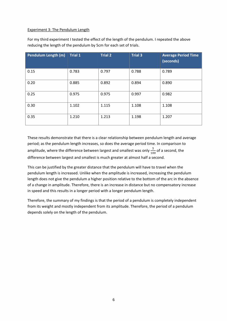
Experiment 3: The Pendulum Length

For my third experiment I tested the effect of the length of the pendulum. I repeated the above reducing the length of the pendulum by 5cm for each set of trials.

Pendulum Length (m) Trial 1 Trial 2 Trial 3 Average Period Time (seconds)

0.15 0.783 0.797 0.788 0.789

0.20 0.885 0.892 0.894 0.890

0.25 0.975 0.975 0.997 0.982

0.30 1.102 1.115 1.108 1.108

0.35 1.210 1.213 1.198 1.207

These results demonstrate that there is a clear relationship between pendulum length and average period; as the pendulum length increases, so does the average period time. In comparison to

amplitude, where the difference between largest and smallest was only 5100

of a second, the

difference between largest and smallest is much greater at almost half a second.

This can be justified by the greater distance that the pendulum will have to travel when the pendulum length is increased. Unlike when the amplitude is increased, increasing the pendulum length does not give the pendulum a higher position relative to the bottom of the arc in the absence of a change in amplitude. Therefore, there is an increase in distance but no compensatory increase in speed and this results in a longer period with a longer pendulum length.

Therefore, the summary of my findings is that the period of a pendulum is completely independent from its weight and mostly independent from its amplitude. Therefore, the period of a pendulum depends solely on the length of the pendulum.

7

Mathematics based on the experiment

Having determined that only the length of a pendulum affects its period I am now focusing solely on those results.

I used the results obtained from the experiment to plot a graph showing the relationship between period time and pendulum length.

Looking at this my first thought was that there was a directly proportional relationship between pendulum length and period. However, I quickly realised that this would lead to the ludicrous result of a pendulum with length 0 having a period of around half a second. Therefore I added the logical point (0,0).

0

0.05

0.1

0.15

0.2

0.25

0.3

0.35

0.4

0 0.2 0.4 0.6 0.8 1 1.2 1.4

Pendulum Length (m)

Time (s)

Fig. 4 – First graph showing the relationship between period time and pendulum length

0

0.05

0.1

0.15

0.2

0.25

0.3

0.35

0.4

0 0.2 0.4 0.6 0.8 1 1.2 1.4

Pendulum Length (m)

Time (s)

Fig. 5 – Second graph showing the relationship between period time and pendulum length with added point (0,0)

8

R² = 0.9973

-0.05

0

0.05

0.1

0.15

0.2

0.25

0.3

0.35

0.4

0 0.2 0.4 0.6 0.8 1 1.2 1.4

Pendulum Length (m)

Time (s)

With the added point I could see a quadratic curve which I marked in using excel. Therefore, I determined that there was a relationship between pendulum length (𝐿𝐿) and a quadratic involving period time (𝑇)

Therefore, 𝐿𝐿 = 𝑎𝑎𝑇2 + 𝑏𝑇 where 𝑎𝑎 and 𝑏 are unknown constants and 𝐿𝐿 represents pendulum length and 𝑇 represents period time.

To find unknown constants 𝑎𝑎 and 𝑏 I substituted two pairs of corresponding values for 𝐿𝐿 and 𝑇 into the above equation.

(0.15) = 𝑎𝑎(0.789)2 + 𝑏(0.789)

(0.35) = 𝑎𝑎(1.207)2 + 𝑏(1.207)

I then solved simultaneously by elimination to get the result:

𝑎𝑎 = 0.239 … and 𝑏 = 0.00162 …

∴ 𝑎𝑎 = 0.24 (to 2 d.p.) and 𝑏 = 0.0016 (to 4 d.p.)

For my purposes, 𝑏 is such a small value that it can effectively be ignored.

Therefore, the relationship between 𝐿𝐿 and 𝑇, where L is the length of the pendulum and T is the period, can be written:

𝑳 = 𝟎.𝟐𝟒𝑻𝟐

Fig. 6 – Third graph showing the relationship between period time and pendulum length with added curve of best fit

9

Limitations

Though I conducted the experiment as carefully as I was able, there were a number of limitations that make the results of the formula derived above somewhat unreliable.

1. It was difficult to ensure that the pendulum swung along a perfect arc in a single plane. Sometimes the pendulum would move more elliptically. This could definitely have an effect on recorded results.

2. I did not have access to particularly precise measuring tools which means that my times, lengths and angles may not be particularly accurate.

3. I was unable to measure my masses and therefore had to assume that they were uniform. While this is not a particularly unreasonable assumption it would have been better had I been able to measure them.

4. I only had a limited number of masses and therefore my results are not as reliable as they would be had I been able to use a larger range.

Despite these limitations I hope that the formula above will prove to be a reasonable reflection of the relationship between pendulum length and pendulum period.

10

The Model

Having derived a formula from experimentation, I intend to test this using a mathematical model to come up with an ‘ideal’ equation demonstrating the relationship between the length and period of a pendulum.

The Assumptions

1. Friction and Air resistance are negligible 2. The pendulum does not swing elliptically (as it sometimes did in the experiment) – it swings

only in one plane. 3. The arm (pendulum length) is a light, inextensible rod.

Variables and Constants

𝐿𝐿 – The length of the pendulum, this is also the radius of the arc along which the pendulum moves

𝜃𝜃 – The angle drawn between the pendulum length and the vertical

𝜔𝜔 – angular velocity

𝑚𝑚 – mass of the pendulum bob

𝑚𝑚 – acceleration due to gravity, will be used as 9.81 𝑚𝑚/𝑠2

𝑣 – velocity

11

Newton’s 2nd Law

This force diagram shows the relevant forces present on a pendulum with angle of release 𝜃𝜃. 𝑚𝑚𝑚𝑚 is the weight of the pendulum due to gravity and 𝑚𝑚𝑚𝑚 sin𝜃𝜃 is the effect of gravity in the direction tangential to the arc of the pendulum.

From the force diagram 𝐹 = −𝑚𝑚𝑚𝑚 sin𝜃𝜃.

From Newton’s 2nd Law 𝐹 = 𝑚𝑚𝑎𝑎.

∴ 𝑎𝑎 = −𝑚𝑚 sin𝜃𝜃 - from comparing the two equations.

For small angles, sin 𝜃𝜃 ≈ 𝜃𝜃

∴ 𝑎𝑎 = −𝑚𝑚𝜃𝜃 This is Acceleration Equation 1 and will be used later in the calculations.

With pendulums, the vertical line tends to be considered as 0. Therefore, any displacement and movement to the right is considered positive and any movement to the left is considered negative. 𝐿𝐿

𝑚𝑚𝑚𝑚

𝑚𝑚𝑚𝑚 sin𝜃𝜃

𝜃𝜃

𝑎𝑎𝑎𝑎𝑎𝑎.

The negative sign comes from travelling opposite to the marked direction of acceleration on the diagram.

12

The Small Angle Approximation

As mentioned above, for small angles, sin𝜃𝜃 ≈ 𝜃𝜃. This fact is nicely demonstrated by Fig. 7.

From the diagram you can clearly see that up until approximately 0.4𝑐𝑐 the graphs lie almost directly on top of one another. However, they quickly separate after this point.

In my opinion, I think using the image of the unit circle helps explain why this is true.

When 𝜃𝜃 is large, as in Fig. 8, there is a large distance between sin𝜃𝜃 and the arc length and they are not a similar size at all. Given that, when we are using radians, the arc length is 𝜃𝜃 this can be used to demonstrate that, for large angles, sin 𝜃𝜃 is not approximately equal to 𝜃𝜃.

However, if you consider Fig. 9 where 𝜃𝜃 is small, you can see that sin𝜃𝜃 and the arc length are almost on top of one another and will be quite similar in length. Given that, once again, the arc length is 𝜃𝜃, this shows that sin𝜃𝜃 ≈ 𝜃𝜃.

I like using the unit circle in this situation because it provides a nice visual demonstration of why sin𝜃𝜃 ≈ 𝜃𝜃 for small angles but not large ones.

1 𝜽𝜽

𝐬𝐬𝐬𝐬𝐬𝐬𝜽𝜽 1

𝑨𝑨𝑨𝑨𝑨𝑨 𝒍𝒍𝒍𝒍𝒍𝒍𝒍𝒍𝒍𝒍𝒍𝒍= 𝟏𝟏 ∙ 𝜽𝜽= 𝜽𝜽

𝜽𝜽

𝐬𝐬𝐬𝐬𝐬𝐬𝜽𝜽

𝑨𝑨𝑨𝑨𝑨𝑨 𝒍𝒍𝒍𝒍𝒍𝒍𝒍𝒍𝒍𝒍𝒍𝒍= 𝟏𝟏 ∙ 𝜽𝜽= 𝜽𝜽

Fig. 7. http://home2.fvcc.edu/~dhicketh/DiffEqns/Spring2012Projects/PendulumPaper/simplepen.pdf

Fig. 8 Fig. 9

13

𝜃𝜃

Simple Harmonic Motion

Simple Harmonic Motion (SHM) is when the restoring force, which pulls the pendulum back to equilibrium – to the vertical, is directly proportional to and acts in the opposite direction of the displacement.

In this case, the restoring force is 𝑚𝑚𝑚𝑚 sin𝜃𝜃 as this is the unbalanced force that pulls the pendulum back to the vertical. However, looking at the force diagram below, you can tell that it does not act in the opposite direction of displacement and therefore a pendulum is not truly modelled by SHM.

This said SHM can be used as an approximation for the motion of the simple pendulum when you have small angles. Similarly as for sin𝜃𝜃 ≈ 𝜃𝜃, I justify this by reference to the fact that when you have very small angles the arc that joins the two corners is very nearly the same as the straight line that joins them. In Fig. 10, the red line and the blue line are very similar and the smaller 𝜃𝜃 gets, the more similar they will be.

The same applies here even though we are considering the perpendicular distance from the vertical point because that is simply half of what Fig. 10 shows.

In addition to acceleration caused by 𝑚𝑚𝑚𝑚, there is the centripetal acceleration, 𝑎𝑎𝑐𝑐, which acts towards the centre and is caused by the tension in the rope that keeps the pendulum moving along a circular path. In the absence of this, the pendulum would simply continue moving in the direction of 𝑚𝑚𝑚𝑚 sin𝜃𝜃.

𝑎𝑎𝑐𝑐 = 𝜔𝜔2𝐿𝐿 where 𝜔𝜔 is angular velocity.

Angular velocity is just like normal velocity except that instead of measuring distance by reference to length it measures it by reference to angle.

𝑚𝑚𝑚𝑚

𝑚𝑚𝑚𝑚 sin𝜃𝜃

𝜃𝜃

𝑎𝑎𝑐𝑐 = 𝜔𝜔2𝐿𝐿

𝑎𝑎𝑐𝑐 = 𝐶𝐶𝐶𝐶𝐶𝐶𝐶𝐶𝐶𝐶𝐶𝐶𝐶𝐶𝐶𝐶𝐶𝐶𝑎𝑎𝐶𝐶 𝐴𝐴𝑎𝑎𝑎𝑎𝐶𝐶𝐶𝐶𝐶𝐶𝐶𝐶𝑎𝑎𝐶𝐶𝐶𝐶𝐴𝐴𝐶𝐶

𝑎𝑎 = 𝜔𝜔2𝐿𝐿 sin𝜃𝜃

𝑎𝑎𝑎𝑎𝑎𝑎.

Fig. 10

𝐿𝐿

14

This result will be proved below.

Firstly, the magnitude of 𝑣 is speed which is simply change in distance ÷ change in time. Therefore,

𝒗𝒗 = 𝒅𝒅𝒅𝒅𝒅𝒅𝒍𝒍

. (1)

When in radians, 𝑎𝑎𝐶𝐶𝑎𝑎 𝐶𝐶𝐶𝐶𝐶𝐶𝑚𝑚𝐶𝐶ℎ = 𝐶𝐶𝑎𝑎𝑑𝐶𝐶𝑢𝑠 × 𝜃𝜃. Therefore, 𝒅𝒅𝒅𝒅 = 𝑳𝒅𝒅𝜽𝜽. (2)

To find the acceleration we will need the change in velocity. Given that 𝑣 is marked as vectors we can simply set them end to end.

Given that 𝑑𝜃𝜃 is very small, the arc is a good approximation to 𝑑𝑣.

Therefore, 𝒅𝒅𝒗𝒗 = 𝒗𝒗𝒅𝒅𝜽𝜽 (3)

If you substitute (2) into (1) you get 𝑣 = 𝐿𝐿 𝑑𝜃𝑑𝑡

.

You can then rearrange this for 𝑑𝜃𝜃 and substitute it into (3) which, after simplification, leaves you with:

(𝒂𝑨𝑨 =) 𝒅𝒅𝒗𝒗𝒅𝒅𝒍𝒍

= 𝒗𝒗𝟐

𝑳

When in radians, to get from angular displacement to arc displacement you multiply by the radius, in this case 𝐿𝐿. The same principles can be used to get from angular velocity to the velocity at the circumference.

∴ 𝑣 = 𝜔𝜔𝐿𝐿

If we substitute this into the expression for centripetal acceleration we get 𝒂𝑨𝑨 = 𝝎𝟐𝑳.

𝒗𝒗 𝒅𝒅𝜽𝜽

𝒗𝒗

Displacement= 𝒅𝒅𝒅𝒅 in time 𝒅𝒅𝒍𝒍

𝒅𝒅𝒅𝒅

𝐿𝐿

𝒗𝒗

𝒗𝒗 𝒅𝒅𝜽𝜽

𝒅𝒅𝒗𝒗

Acceleration is change in velocity over change in time. Therefore, the centripetal acceleration will be equal to 𝑑𝑣𝑑𝑡

.

This diagram shows the velocity of an object moving in a circle at two different points.

The object has moved through the very small angle 𝑑𝜃𝜃 and covered correspondingly small distance 𝑑𝑥 in time 𝑑𝐶𝐶.

Using this information, a number of equations can be formed.

15

𝜃𝜃

𝑎𝑎𝑐𝑐 = 𝜔𝜔2𝐿𝐿

𝑎𝑎 = 𝜔𝜔2𝐿𝐿 sin𝜃𝜃

𝑎𝑎𝑎𝑎𝑎𝑎.

N.B. we find the centripetal acceleration in terms of 𝜔𝜔 because this relates to 𝜃𝜃 which is present in the first acceleration equation as opposed to arc length which is not.

Now that this result has been proven, you can simply resolve it into its components to find the target acceleration, 𝑎𝑎, which runs perpendicular to the vertical. (Marked in blue on the force diagram)

This gives you 𝑎𝑎 = −𝜔𝜔2𝐿𝐿 sin𝜃𝜃.

However, once again, sin𝜃𝜃 ≈ 𝜃𝜃,

∴ 𝑎𝑎 = −𝜔𝜔2𝐿𝐿𝜃𝜃

Now we can use both equations to derive a formula for the period of a pendulum, 𝑇.

Acceleration Equation 1: 𝑎𝑎 = −𝑚𝑚𝜃𝜃

Acceleration Equation 2: 𝑎𝑎 = −𝜔𝜔2𝐿𝐿𝜃𝜃

From comparison, 𝜔𝜔2𝐿𝐿 = 𝑚𝑚

∴ 𝜔𝜔 = �𝑔𝐿

Due to the SHM approximation, the motion of a pendulum, which does not move at a constant velocity, can be modelled by an object moving at a constant velocity around a circle with a radius that is equal to the horizontal displacement of the pendulum. (i.e. from the vertical to the point of release)

Therefore the period of the pendulum is equal to the time it takes for the object to move about the entire circle.

Given that there are 2𝜋𝑐𝑐 in a circle, 𝜔𝜔 = � 𝑎𝑛𝑔𝑙𝑒𝑡𝑖𝑚𝑒 𝑡𝑎𝑘𝑒𝑛

� = 2𝜋𝑇

.

Therefore, 𝜔𝜔 can be substituted for 2𝜋𝑇

.

∴ 2𝜋𝑇

= �𝑔𝐿

Following this, we simply rearrange to make 𝑇 the subject which gives us:

𝑻 = 𝟐𝝅�𝑳𝒍𝒍

which is the established result for finding the period of a pendulum using the small angle approximation.

This is Acceleration Equation 2.

16

Comparison

From mathematical model:

𝑇 = 2𝜋�𝐿𝐿𝑚𝑚

∴ 𝐿𝐿 =𝑚𝑚

(2𝜋)2𝑇2

𝑚𝑚 = 9.81𝑚𝑚/𝑠2

∴ 𝐿𝐿 = 0.248𝑇2

Solution

𝑇 = 1𝑠

𝐿𝐿 =𝑚𝑚

(2𝜋)2𝑇2

𝐿𝐿 =𝑚𝑚

(2𝜋)2(1)2

𝐿𝐿 = 0.248 𝑚𝑚

From experimental data:

𝐿𝐿 = 0.24𝑇2

This demonstrates that experimental data and the mathematical model produce almost exactly the same result.

This seems to justify the mathematical formula as well as my experimental method.

𝑇 = 2𝑠

𝐿𝐿 =𝑚𝑚

(2𝜋)2𝑇2

𝐿𝐿 =𝑚𝑚

(2𝜋)2(2)2

𝐿𝐿 = 0.994 𝑚𝑚

Therefore, to create a pendulum that could be used in a pendulum clock you will need a pendulum length of 0.248m for a period of 1 second or a pendulum length of 0.994m for a period of 2 seconds. The mass of the pendulum does not matter however, given that this model assumes that air resistance and friction are negligible it would be sensible to design the pendulum in such a way that friction and air resistance are minimised.

17

Conclusions and Limitations

The biggest limitation of my derived formula is that it is only an approximation. The use of SHM and the small angle approximation is reasonably effective and makes the mathematics far more accessible than it is otherwise but will not produce very accurate results, particularly at larger angles as demonstrated by Fig. 11.

This said it is an excellent approximation at smaller angles (see Fig. 12) which is why it was used for so long. Pendulum clocks used to lose around 15 seconds per day due to the use of the small angle approximation which was still a vast improvement on previous technology.

Fig. 11 http://home2.fvcc.edu/~dhicketh/DiffEqns/Spring2012Projects/PendulumPaper/simplepen.pdf

Fig. 12 http://home2.fvcc.edu/~dhicketh/DiffEqns/Spring2012Projects/PendulumPaper/simplepen.pdf

18

The other limitation to consider is that the derived formula does not account for friction or air resistance and therefore might be slightly inaccurate. However, friction and air resistance genuinely have little effect on the period of a pendulum – a pendulum can continue to swing for a surprisingly long time even in the absence of external forces – therefore, this is not a particularly significant limitation.

Ultimately I consider my model successful as I was able to develop the established result for the relationship between pendulum length and pendulum period.

This formula can either be used to find the length required for a certain period, as I have done, or it can be used to predict the period of a pendulum with a known length.

A slightly more unusual use is that, due to the nature of the equation, you can use an experiment, to get values for L and T, and the formula to prove the value for gravitational acceleration or even find out the value of acceleration due to gravity on another planet!

19

Resources

https://en.wikipedia.org/?title=Pendulum_clock

http://home2.fvcc.edu/~dhicketh/DiffEqns/Spring2012Projects/PendulumPaper/simplepen.pdf

http://hyperphysics.phy-astr.gsu.edu/hbase/pend.html#c3

https://www.youtube.com/watch?v=VKUqieD2R9s

https://www.youtube.com/watch?v=7YwBNRuBvjw

https://www.youtube.com/playlist?list=PLnw1pIhtIsyJDucHsusJkugAHyp4pynUy