Helsinki University of TechnologyInformation and Computer Systems in Automation

Espoo 2004 Report 10

Modelling Industrial Maintenance Systems and the Effects ofAutomatic Condition Monitoring

Tuomo Honkanen

TEKNILLINEN KORKEAKOULUTEKNISKA HÖGSKOLANHELSINKI UNIVERSITY OF TECHNOLOGYTECHNISCHE UNIVERSITÄT HELSINKIUNIVERSITE DE TECHNOLOGIE D´HELSINKI

Production Rate40

35

30

25

20

3 3

3 3

3

3

3

3

3 33

33

3

3

33

3

3

33

3

33

3

3

2 22

2

2

22

2

2 2 22 2

2

2

2

2

2

2

22

2

2

22

2

2

1 1 1

11

1

1

1

11

1 1

1

1

11

1 1

1

1

11

1

11

1

1

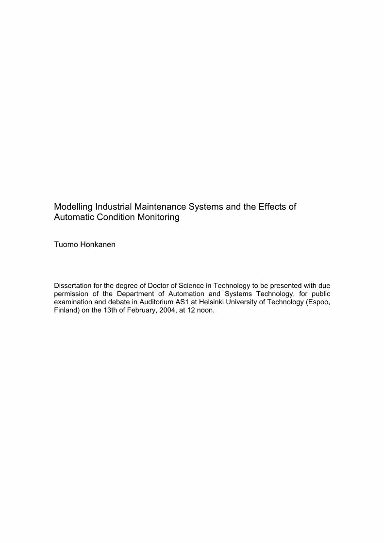
0 73 146 219 292 365 438 511 584 657 730Time (Day)

Production Rate : items/Day1 1 1 1 1 1 1 1 1 1 1 1 1 1 1 1 1 1 1Production Rate : Random items/Day2 2 2 2 2 2 2 2 2 2 2 2 2 2 2 2 2 2Production Rate : Random Monit items/Day3 3 3 3 3 3 3 3 3 3 3 3 3 3 3 3

Modelling Industrial Maintenance Systems and the Effects ofAutomatic Condition Monitoring

Tuomo Honkanen

Dissertation for the degree of Doctor of Science in Technology to be presented with duepermission of the Department of Automation and Systems Technology, for publicexamination and debate in Auditorium AS1 at Helsinki University of Technology (Espoo,Finland) on the 13th of February, 2004, at 12 noon.

Distribution:Helsinki University of TechnologyDepartment of Automation and Systems TechnologyInformation and Computer Systems in Automation

P.O. Box 5500

FIN-02015 HUT, Finland

Tel. +358-9-451 5462

Fax. +358-9-451 5394

© Tuomo Honkanen

ISBN 951-22-6815-9

ISBN 951-22-6816-7 (PDF)

ISSN 1456-0887

Picaset Oy

Helsinki 2004

3

ABSTRACT

In this dissertation, industrial maintenance activities are researched from a systemic point ofview. Maintenance is considered from the selected viewpoint as a control system for controllingthe reliability of machines in a process environment. The control takes place throughcommunication of information. Thus, maintenance can also be considered as an informationprocessing system. Therefore, the viewpoint also supports development of future maintenanceinformation systems. The specific interest of the research is in modelling the effects of automaticcondition monitoring systems enabled by embedded electronics and software in industrialmachines.

The research problem is to model maintenance systems and the effects of conditionmonitoring. Because the focus is on the maintenance systems, the research approach differs fromthe usual reliability engineering approaches, which focus on the reliability of mechanicalsystems. The applied methods are a literature study of the main reliability paradigms and thesystems theory to derive a theory of maintenance systems. The theory is then applied bydeveloping a UML knowledge model, an applied Gorry-Morton control activities model, astochastic simulation model and a dynamic simulation model of the maintenance systems. Also,one additional simulation model is developed to study the effect of remote condition monitoringon the spare parts supply chain.

The main results indicate that the subjective nature of failures, the available informationabout the machines as well as the repeatability of the maintenance actions are the most importantfactors in the maintenance system control. Also, correct selection of the maintenance system costfunctions is critical in determining the applied maintenance policies.

Condition monitoring increases observability of the states of the machines and thereforeenables more effective maintenance systems with the help of condition-based maintenance.However, the effectiveness of condition-based maintenance depends on the accuracy of themonitoring and the coverage of the failure diagnosis. The failure patterns and the repeatability ofthe maintenance actions also contribute significantly to the effectiveness of condition-basedmaintenance. In spare parts supply chains, remote condition monitoring can be used to stabilisethe supply chain variability and to reduce the supply chain sensitivity to random noise andsudden changes in the consumption.

Keywords: maintenance system, condition monitoring, condition-based maintenance, supplychain, information system

4

ACKNOWLEDGEMENTS

The work presented in the thesis was carried out at Metso Corporation during the years 2002 and2003. I express my gratitude to my professor Kari Koskinen and my advisor Dr. Jouni Pyötsiäfor providing guidance and pushing me forward during my research. I warmly thank MikaNissinen, Arto Marttinen, Ismo Platan, and Håkan Renlud from Metso Corporation for helpingwith the dissertation and for the facilities support. The financial support from HelsinkiUniversity of Technology and Neles 30-year Anniversary Foundation is gratefullyacknowledged. I also thank the pre-examiners of the thesis, Doctor Urho Pulkkinen, andProfessor Seppo Virtanen, who gave valuable comments on the first version of the manuscript.

Finally, my loving thanks to my wife Outi and my daughter Linda for giving me joy and supportfor the numerous days with this research.

Helsinki, October 13th, 2003Tuomo Honkanen

Quidquid latine dictum sit, altum viditure.

5

CONTENTS

Abstract .........................................................................................................................................3

Acknowledgements .......................................................................................................................4

Contents .........................................................................................................................................5

Abbreviations, symbols and glossary ..........................................................................................8

1 Introduction and overview ................................................................................................11

1.1 Motivation and background .........................................................................................11

1.2 Problem setting and goals of the study ........................................................................11

1.3 Research approach, methodology and design .............................................................12

1.4 Modelling methodologies...............................................................................................13

1.5 Included industries of the research ..............................................................................13

2 Background interviews and observations ........................................................................14

2.1 Interviews .......................................................................................................................142.1.1 Business drivers .................................................................................................................. 142.1.2 Computerised maintenance management ............................................................................ 142.1.3 Manufacturer and user-perceived failures and design criteria for machines ....................... 152.1.4 Preventive replacement policies and condition monitoring ................................................ 15

2.2 Observations of discussion in the mailing list of reliabilityweb.com.........................15

2.3 Summary of interviews and reliabilityweb.com observations ...................................17

3 Scoping of the research......................................................................................................18

4 Review of reliability and maintenance literature ............................................................20

4.1 Terminology ...................................................................................................................20

4.2 Reliability paradigms ....................................................................................................204.2.1 Reliability-centered maintenance ........................................................................................ 214.2.2 Total productive maintenance ............................................................................................. 224.2.3 Reliability engineering ........................................................................................................ 234.2.4 Control engineering............................................................................................................. 244.2.5 Summary of paradigms ....................................................................................................... 24

4.3 Maintenance Processes..................................................................................................25

4.4 Business aspects .............................................................................................................284.4.1 The costs and revenues of maintenance .............................................................................. 28

5 Systems approach to maintenance....................................................................................30

5.1 Systems ...........................................................................................................................305.1.1 Functions, structures and environments .............................................................................. 305.1.2 Complexity and interdependencies ..................................................................................... 315.1.3 Factoring and integrating systems....................................................................................... 315.1.4 Control systems................................................................................................................... 325.1.5 Maintenance activities as a system...................................................................................... 325.1.6 Machine reliability and maintenance system effectiveness................................................. 335.1.7 Summary ............................................................................................................................. 34

5.2 Maintenance system performance metrics ..................................................................345.2.1 Efficiency and effectiveness................................................................................................ 345.2.2 Overall Equipment Efficiency............................................................................................. 355.2.3 Availability.......................................................................................................................... 35

6

5.2.4 Proposed effectiveness and efficiency metrics.................................................................... 365.2.5 Availability of source data for the metrics .......................................................................... 37

5.3 Failures ...........................................................................................................................375.3.1 Failure states ....................................................................................................................... 375.3.2 Failure patterns.................................................................................................................... 385.3.3 Failure causes and effects.................................................................................................... 395.3.4 Partial failures ..................................................................................................................... 395.3.5 Subjective state definitions in the maintenance paradigms ................................................. 40

5.4 Effects of information in failure and maintenance processes ....................................415.4.1 The observability and reversibility of black-box system states........................................... 415.4.2 Condition monitoring .......................................................................................................... 415.4.3 Condition-based maintenance actions ................................................................................. 435.4.4 Information creation in failure and maintenance processes ................................................ 43

6 System models I-V..............................................................................................................45

6.1 Overview of system models I-V ....................................................................................45

6.2 System model I: A UML domain model of failure and maintenance concepts .......456.2.1 Purpose of the model........................................................................................................... 456.2.2 Knowledge, ontology and information communication ...................................................... 466.2.3 UML as a knowledge modelling methodology ................................................................... 466.2.4 Validation of the UML model with a knowledge modelling tool ....................................... 466.2.5 The UML domain model..................................................................................................... 476.2.6 Summary ............................................................................................................................. 51

6.3 System model II: A Gorry-Morton information systems framework.......................516.3.1 Purpose of the model........................................................................................................... 516.3.2 Artificial intelligence .......................................................................................................... 526.3.3 The Gorry-Morton framework ............................................................................................ 526.3.4 Applying the Gorry-Morton framework to maintenance systems....................................... 53

6.4 System model III: A stochastic maintenance system simulation model....................556.4.1 Purpose of the model........................................................................................................... 556.4.2 Overview and assumptions.................................................................................................. 556.4.3 Numerical method of a preventively maintained system .................................................... 566.4.4 Simulation model of a preventively maintained system under condition monitoring ......... 586.4.5 Simulation results................................................................................................................ 606.4.6 The effect of limited time to diagnose................................................................................. 626.4.7 Summary ............................................................................................................................. 62

6.5 System model IV: A dynamic maintenance system simulation model......................626.5.1 Purpose of the model........................................................................................................... 626.5.2 Dynamic modelling............................................................................................................. 636.5.3 Simplifications and assumptions in dynamic modelling ..................................................... 636.5.4 Model overview .................................................................................................................. 646.5.5 Component failure and maintenance model ........................................................................ 646.5.6 Worker allocation model..................................................................................................... 666.5.7 Deterioration failure process ............................................................................................... 676.5.8 Repair process ..................................................................................................................... 686.5.9 Repeatability of repair actions............................................................................................. 686.5.10 Condition-based maintenance process ................................................................................ 686.5.11 Preventive maintenance process.......................................................................................... 686.5.12 Preventive maintenance control model ............................................................................... 696.5.13 Analysis of the system behaviour........................................................................................ 716.5.14 The effect of repair and maintenance repeatability on the system dynamics ...................... 736.5.15 The effect of condition monitoring on the system dynamics .............................................. 746.5.16 The effect of insufficient work resources on the system dynamics..................................... 75

6.6 System model V: A dynamic spare parts supply chain simulation model................766.6.1 Purpose of the model........................................................................................................... 766.6.2 Spare parts demand as a stochastic process......................................................................... 766.6.3 Modelling supply chains ..................................................................................................... 78

7

6.6.4 Model overview .................................................................................................................. 796.6.5 A study of the system dynamics.......................................................................................... 826.6.6 Step response results in the normal supply chain mode ...................................................... 826.6.7 Step response results in the informed and fully informed mode ......................................... 836.6.8 Random data responses in the informed and fully informed modes ................................... 856.6.9 Further considerations......................................................................................................... 876.6.10 Summary and comparison to the results of other similar studies ........................................ 88

7 Discussion and conclusions................................................................................................89

7.1 Summary of maintenance systems control ..................................................................89

7.2 The effect of condition monitoring on maintenance systems .....................................90

7.3 The ability of the simulation models to predict maintenance systems behaviour....90

7.4 Future directions and issues .........................................................................................91

References....................................................................................................................................92

Appendix A: Interviews .............................................................................................................98

Appendix B: Model III in Mathcad 2001i format..................................................................100

Appendix C: Model IV in Vensim 5.0 text format.................................................................109

Appendix D: Model V consumption analysis in Mathcad 2001i format..............................112

Appendix E: Model V in Vensim 5.0 text format...................................................................116

8

ABBREVIATIONS, SYMBOLS ANDGLOSSARY

ABBREVIATIONS IN THE TEXT

AI artificial intelligenceCBM condition-based maintenance, a synonym for predictive

maintenanceCE control engineeringCM condition monitoringCMMS computerised maintenance management systemEOQ economic order quantityFMEA failure modes and effects analysisFTA fault tree analysisMTBM mean operating time between maintenanceMTTAM mean operating time to arrange a maintenance breakMTTF mean operating time to failure of a function or a machineMTTFR mean calendar time to reach first repaired failureMTTM mean calendar time to maintainMTTR mean calendar time to repairOEE overall equipment efficiencyPM preventive maintenanceRE reliability engineeringRCM / RCM II reliability-centered maintenanceTPM total productive maintenanceTTF operating time to failureUML unified modelling languageUP unified process

9

SYMBOLS AND VARIABLES IN EQUATIONS

α Gamma distribution scale parameterβ Weibull distribution shape parameterη Weibull distribution scale parameterλ average failure rate, failure rateµgroup average failure interval of a group of machinesAo operational availabilityC total number of componentsc number of working componentsCi cost of one inspectionCa actual daily consumptioncco component pricecre repair work costscma proactive maintenance costscdcap daily lost capacity expenses of proactive maintenancecdop daily increased operating expenses caused by a failurecdqu daily increased quality expenses caused by a failurecdcar daily lost capacity expenses caused by a failureDe estimated daily demandDC diagnostics coverageDT failure detection timeE reliability target errorEOQ economic order quantityfc cost function of maintenance and failuresGp proportional error gainGi integral error gainK safety factorn number of proactive maintenance actions in a yearnfd the number of components failed because of deteriorationnfi the number of components failed because of infant failuresnr the number of components being repairedm number of repairs in a yearmf number of preventive maintenance actions per failureMTBI mean operating time between inspectionsMTBM mean operating time between maintenance, a synonym for MTTFMTTAM mean operating time to arrange a maintenance breakMTTF mean operating time to failureMTTFR mean calendar time to reach first repaired failureMTTM mean calendar time to maintainMTTR mean calendar time to repairOEE overall equipment efficiencyOQ order quantityS reliability target setpoint, system stateT time to failureTm time to failure of a maintained system or machineTd transportation or production delayTTF operating time to failureUt machine utilisation of calendar timeY controlled reliability variable

10

GLOSSARY

asset in the context of industrial maintenance, an asset is physicalproperty invested for production purposes

availability the probability that at any given instant of time, including orexcluding the proactive maintenance, a machine is not failed

controllability the ability to control the reliability of the machine in order toachieve and maintain some specific maintenance system efficiencylevel1

diagnostics coverage the probability that a failure state is detected correctly by adiagnostics system, see also observability

failure a state of a machine in which the machine is not performing arequired function at the required level

failure event in this dissertation, an interchangeable term for failure modefailure mode any event which causes a functional failurefailure pattern a failure rate pattern as a function of operation timefailure state see failurefault an existence (state) or an occurrence (event) of a failure or a

potential failuremaintenance the combination of all technical and administrative actions,

including supervision actions, intended to retain an entity in, orrestore it to, a state in which it can perform a required function(IEC 60050-191, 1996)

maintenance policy a decision to apply reactive, preventive or condition-basedmaintenance

maintenance program a formal proactive maintenance plan for machinesmaintenance strategy a long-term company strategy to use some combination of various

maintenance policies and reliability paradigmsobservability the probability that a system state is detected correctlypartial failure partial loss of machine functionplanned maintenance maintenance action with planned procedures and resource needspredictive maintenance a proactive maintenance action triggered by condition monitoringpreventive maintenance a proactive maintenance action executed in order to prevent a

failureproactive maintenance maintenance action executed before occurrence of an individual

failurerepeatability the probability that any maintenance action of certain action type

results always in the same target system statereactive maintenance maintenance action executed after occurrence of individual failurereliability the probability that a machine does not fail during a given time

intervalreliability paradigm a theoretical framework of a scientific school or discipline in

maintenance or reliabilityscheduled maintenance time-scheduled proactive maintenance actiontotal failure total loss of a machine functionunplanned maintenance a proactive or reactive maintenance action with maintenance

procedures and resource needs not planned before executing themaintenance task

1 Note that the definition of controllability differs from the mathematical definition (Wolovich, 2000) in mathematicalcontrol theory.

11

1 INTRODUCTION AND OVERVIEW

1.1 MOTIVATION AND BACKGROUND

I have been working with automation and industrial information technology for eight years.During these years I have been involved in several development projects that aim for automaticmachine condition monitoring (Honkanen, 1997) and machine data communications.Technically these projects have succeeded: the developed information systems have beentechnically modern and worked well. However, despite all the technical advantages theseproducts have not been commercial successes.

Some years ago I noticed that a good business process consultant can achieve commerciallymuch more successful results by just capturing the business requirements and doing a thoroughanalysis of the business processes before developing anything. I had forgotten that the wordinformation in the information technology really refers to the substance of an informationsystem.

An automatic condition monitoring system is essentially such an information system. Theinformation in the system exists to be processed by humans and computers in order to serve apurpose. The other technologies that relate to automatic condition monitoring includeapplications in automatic machine failure diagnostics, failure prognostics, maintenance planning,and such future concepts as automatic spare parts orders from intelligent machines. All theseactivities interrelate to increase the efficiency of industrial production processes andmaintenance.

The real problem was that I did not know the big picture, I could not find only one such, andno one could draw me one either, to analyse the effects of automatic condition monitoring onindustrial maintenance activities.

1.2 PROBLEM SETTING AND GOALS OF THE STUDY

Some investment machine manufacturing companies have developed concepts (ABB, 2002;Metso, 2002) that aim at providing totally integrated information systems. According to theirvision, in the future it will be possible to automate and integrate the maintenance activities in asystem that consists of the machines, persons and information systems. New technologies, suchas electronics, mechatronics, communication and software technologies make it possible todevelop intelligent machines and condition monitoring systems. The problem is how to find thebest application areas for such technologies.

This dissertation proposes that thinking industrial maintenance as an information processingsystem leads to a top-down view that helps in analysing the effects of automatic conditionmonitoring.

Therefore, the research problem is to model maintenance systems and the effects of automaticcondition monitoring.

The main problem was divided in sub-problems to make the research problem easier to answer.The three research questions to address the problem can be derived from the systems theoryapproach of Saaty and Kearns (1985):

12

Q1: What is the purpose of maintenance?Q2: What are the structures, behaviour and the information flows in the maintenance systems?Q3: How does condition monitoring affect the systems?

The questions, Q1-Q3, form a logical top-down chain from the purpose of maintenance to theeffects of the condition monitoring to maintenance systems.

1.3 RESEARCH APPROACH, METHODOLOGY ANDDESIGN

The problem is to model maintenance systems and the effects of automatic condition monitoringon the functions of the maintenance systems. A model of maintenance systems means here somesystem model that is not bound to some single maintenance or reliability paradigm, butapplicable to most common paradigms. The systems approach, which studies the relations,organisation and interactions of entities on an abstract level is proposed to formulate such amodel. Contrasted to analytical approach, which focuses on the parts, the systems approachfocuses on the whole (Schoderbek et al., 1990). This viewpoint emphasises that new scientificknowledge can be generated not only by researching a specific deep and strictly defined problemdomain, but also by studying interrelations and integrating the problem domains.

In general, the “what” problems of questions Q1 and Q2 aim at developing hypotheses andpropositions for further study (Yin, 1994). That is, Q1 and Q2 aim at analysing maintenancesystems. This dissertation is by nature constructive and the analysis was done by a conceptualliterature study to induce the theory of maintenance systems from the existing reliabilityparadigms (Q1-Q2). Weinberg (1975, p. 143) calls this non-observing methodology academicscience with the value of creating ideals not bound to a specific paradigm. Finding analogiesbetween the paradigms makes it possible to generate a theory of maintenance systems that isderived from a family of paradigms. Operating with analogies is a form of inductive logicwithout the necessity of forming its conclusions logically from its premises. The strength of thismethodology in this dissertation is that no specific regional or cultural maintenance paradigmdominates the theory. The main weakness is the possible generality of the theory, which mayincrease the probability of the existence of such a system, but reduce the informative value of themodels based on the theory.

The literature study was aligned by data acquired from interviews and observations ofrepresentatives of industrial companies. The interviews were open and informal attempting toanswer the question: how do/would you use information technology and automatic conditionmonitoring in maintenance processes. The weakness of open and unstructured interviews is thepossibility that the interviewer manipulates the discussion unconsciously. Therefore,observations of discussions at a public discussion forum on the Internet were also used to verifythat the interviews were focused on the right topics. The interviews and observations should notbe considered as giving very high empirical evidence. The companies, subjects and interviewingtimes are presented in Appendix A: Interviews.

The theory of maintenance systems was then used for deriving the models to provideanswers to questions Q2-Q3, and finally the conclusions of the research were derived. Themethodological research approach is shown in Figure 1. It should be noted that the research wassomewhat iterative from theory part to models and back to theory part.

13

Reliability paradigms and systems theoryliterature study

Maintenancesystems theory

Induce

Models

Conclusions

Industry observations and interviews

Verify

Align

Model

Conclude

Figure 1 The methodological approach of the research.

1.4 MODELLING METHODOLOGIES

The focus of the developed theory of maintenance systems is to define and describe themaintenance systems and the boundary conditions for modelling such systems. Mathematicalsystems theory focuses on formal and rigorous quantitative models of systems, whereas appliedsystems theory, or systems technology, focuses on more qualitative, practical applications, suchas software development for specific problems (Laszlo, 1972). The system models sought afterin this dissertation are on the one hand knowledge models of the problem domain of interest, andon the other hand functional models that must be presented as mathematical models. Therefore,both applied systems thinking and quantitative systems modelling are used.

The synthesised maintenance information system theory is presented as figures, tables andwritten text. The knowledge constructs of the theory are presented in a more formalisedknowledge representation format, namely unified modelling language (UML) domain models(Larman, 2002). The control aspects of maintenance systems are captured by mapping theinformation systems framework of Gorry and Morton (1989) to the maintenance activities. Thecost model and stochastic behaviour are modelled with stochastic simulation, and thebehavioural modelling is done with time-dependent dynamic models.

1.5 INCLUDED INDUSTRIES OF THE RESEARCH

Proactive maintenance and reliability are most important in industries where the cost of failures,the failure rates and the cost of maintenance are high (Komonen, 1998). Therefore, thisdissertation applies best to highly integrated process industries, such as pulp and paper orchemical industries. The models and results may be applicable to other industries such asaeronautics and nuclear energy production but these specific application areas are not explicitlyconsidered in the dissertation.

14

2 BACKGROUND INTERVIEWS ANDOBSERVATIONS

As noted in Chapter 1, the observations and interviews should not be considered as empiricalresearch with very high scientific evidence. However, they represent an important source ofinsight and alignment for the research. The interviews and observations are reviewed in thischapter.

2.1 INTERVIEWS

The interviews were unstructured open discussions and held between March 12, 2002 andJanuary 7, 2003. The interviews consisted of 21 interview sessions including 29 differentpersons from 10 different companies. Fourteen interviewees came from Metso Corporationserving mainly the pulp and paper industry. The other interviewees came from the service andinformation technology providers, pulp and paper maintenance management and componentmanufacturers. Because a large proportion of the interviewees was from machine manufacturersand technology providers, the viewpoint is oriented towards machine-suppliers and informationtechnology providers.

The purpose of the interviews was to ask how information technology and remote conditionmonitoring could be used to enhance industrial maintenance activities. A large proportion of thediscussed topics fell either under computerised maintenance management system (CMMS) orremote condition monitoring and failure diagnostics (INTERVIEWS 2, 3, 4, 5.1, 5.2, 6, 8, 9, 10,11, 12, 14, 15.1, 15.2, 16, 18.1, 18.2, 19, 20, 21.1, 21.2, 21.3, 21.4). The general sentimentamong the interviewees was that the application of information technology was expected tobring dramatic results in machine reliability and maintenance process efficiency. At the sametime, most interviewees were unable to show or calculate the benefits of the application ofinformation technologies.

2.1.1 Business drivers

Some interviewees (INTERVIEWS 5.1, 5.2, 11) presented an idea that remote conditionmonitoring might help them bypass the other maintenance companies and help in offeringmaintenance services. The idea is that with condition monitoring the machine manufacturercould get so much information about the condition and operation of the machines, that themachine manufacturer is able to predict the failures and offer the optimal methods to operate themachines. This would change the service business so that the machine manufacturer wouldcontrol the maintenance business with the help of remote condition monitoring. If using an in-house service organisation these technologies were seen as a means to enhance service efficiencyand customer loyalty (INTERVIEWS 3, 4, 5.1, 5.2, 9, 10, 11, 12, 16, 20).

2.1.2 Computerised maintenance management

Interviews with CMMS providers (INTERVIEWS 8, 9, 12) indicated that the CMMS softwarepackages are indeed very large and full of features, such as work-order management, reporting,inventory control, audit trails and much more. The actual problem seems not to be the CMMStechnology but the implementation and usage of the CMMS systems. As an example, a CMMSimplementation project was reported as successful, but only 15 % of the CMMS features weretaken into use. Thus, the problem of implementing information systems to control a maintenance

15

system is related to the structures and operation of the maintenance system rather than to being atechnical problem.

2.1.3 Manufacturer and user-perceived failures and design criteria formachines

Some practical problems arise with the definition of failures. According to the interviewedrepresentatives of an industrial valve manufacturing company (INTERVIEWS 4, 15.1) up to30% of old plant control valves may be non-functional or oscillating and thus failed. Still, theplants produce good-quality products, which means that the valves have not necessarily failedfrom the user perspective.

An interviewed technology director (INTERVIEW 11) of an industrial valve manufacturernoted that equipment specifications are set at the plant design phase, but the specifications areoften too tight or too loose, and seldom describe the real operating point or control limits of theprocess. This was confirmed by the interviewed consulting company representatives(INTERVIEW 18.1, INTERVIEW 18.2). According to them, the process equipment is usuallyoversized in order to be able to increase the plant capacity later. Therefore, the design-phasespecifications cannot be used for defining whether the machine is failed or not.

2.1.4 Preventive replacement policies and condition monitoring

An interviewed industrial valve maintenance manager (INTERVIEW 7) told that the paper andpulp industry customers are often willing to change the whole control valve, instead of changingjust the valve, actuator or positioner even if the failure can be identified to one of thesesubsystems. The interviewee also told that in a petrochemical plant the whole plant is shut downevery four years and every deteriorating and critical component is changed. Similarly, a paperindustry representative (INTERVIEW 17) told that when changing a failed bearing in a papermachine roll, the other bearing is also changed regardless of its age. The reason for the changepolicy is that the additional cost of changing the other bearing as well is low when the whole rollis detached from the machine.

The reasoning of the interviewees seem to represent the ideology that the maintenance staffin these process industries always wants to make certain that the system under maintenance istotally restored. Restoring the system state at certain points of time may help in keeping track ofthe system state and in standardisation of the maintenance activities.

The same paper industry representative (INTERVIEW 17) told that under conditionmonitoring the bearing is changed only if the condition monitoring indicates failure or the age ofthe bearing is exceptionally high. This means that they do not fully trust to condition monitoringsystems.

2.2 OBSERVATIONS OF DISCUSSION IN THE MAILINGLIST OF RELIABILITYWEB.COM

The reliabilityweb.com e-mail discussion list is open for reliability and maintenanceprofessionals. The discussion list is moderated so that commercial e-mails are filtered out quitewell. The observed e-mails were sent between May 1, 2002 and January 25, 2003. During thattime, a total of 497 e-mails were read through, archived and later categorised by reading themthrough one more time. There were 139 message senders from a large number of organisationsaround the world. The viewpoint the e-mail discussion list gives is user-oriented because of the

16

large number of e-mails related to operative and maintenance management topics. The categoriesused in analysing the messages are shown in Table 1.

Category Description of Discussion TopicsCM Automatic and manual condition monitoring methods of machinesCMMS Computerised maintenance management system, maintenance scheduling,

planning and reporting softwareMAINTMGMT.

Labour and cost management methods, job descriptions, cost estimates,maintenance and workforce planning

MATHMODELING

MTBM, MTTF, availability calculations, simulation and Markov models

OPERATIVEMAINT.

Specific machine functional problems, failures, technologies and opinions

PM Preventive maintenance methods, such as lubrication, component changeintervals

RCA Root-cause analysis implementation and usageRCM Reliability-centered maintenance methodologies and implementationTPM Total productive maintenance related issues, such as autonomous

maintenance by operatorsUNRELATED Author's messages (3) and replies to them (1), some commercials, accidental

messages Table 1 Reliabilityweb.com e-mail discussion list categories.

The number of messages and the fraction of total messages in each category are presented inFigure 2.

106

103

78

76

42

36

21

13

13

9

21,3 %

20,7 %

15,7 %

15,3 %

8,5 %

7,2 %

4,2 %

2,6 %

2,6 %

1,8 %

0 20 40 60 80 100 120

OPERATIVE MAINT.

MAINT MGMT

CMMS

CM

RCM

MATH MODELING

UNRELATED

TPM

PM

RCA

Figure 2 Number and percentage of Reliabilityweb.com e-mail discussion list messages bycategory.

During the observation period, the e-mail discussion list was heavily used by maintenancemanagers and also by some reliability consultants. A large number (42.0 %) of the messageswere directly related to maintenance management and practical maintenance and reliabilityproblems, such as selecting the correct maintenance method or tool. The CMMS and conditionmonitoring were also (31.0 %) lively topics.

These messages support the interviews: efficiency and reliability gains are sought fromcondition monitoring and CMMS technologies. Some interest was seen in using hand-held

17

devices in reporting the maintenance actions, but the main CMMS discussion was about howand which CMMS system to implement and how to use a CMMS system. The conditionmonitoring discussion focused much on vibration analysis of bearings and electrical motors.

Compared to total productive maintenance (TPM) (2.6 %) reliability-centered maintenance(RCM) (8.5 %) was also a popular topic. Perhaps the reason was that there were quite manydiscussion participants from the USA, Europe, Australia and South-America where RCM is thedominating paradigm.

Quite surprisingly, several participants were interested in mathematical modelling (7.2 %):reliability, availability and cost calculation methods were raised quite frequently. The motivationfor the calculations was quite obviously to prove the effectiveness of the selected maintenancepolicies and technologies.

Preventive maintenance (2.6 %) was not a popular topic by itself. Probably this does notindicate that preventive maintenance is not interesting or being applied, but the interest wasexpressed under other topics, such as mathematical modelling and discussion related to operativemaintenance. Root-cause analysis (1.8 %) was a topic that could have been categorised undermaintenance management. However, as a specific reliability method it deserves its owncategory.

2.3 SUMMARY OF INTERVIEWS ANDRELIABILITYWEB.COM OBSERVATIONS

Both the interviews and e-mail discussion list indicate that there are two equally interesting areasamong machine manufacturers and users to apply information technology in industrialmaintenance: CMMS and condition monitoring. However, the interviews and observations giveconflicting signals that while the technology providers are trying to develop more and moreadvanced tools, the maintenance departments seem to struggle with daily problems ofimplementing and operating such systems. The technology providers or the users do generallynot know the feasibility of applying these technologies, but apparently they seem to improve theefficiency of the maintenance activities. The users combine their experience and heuristics indefining maintenance policies and in usage of condition monitoring systems. Some help issought from maintenance paradigms such as RCM or TPM. The resulting maintenance systemsseem to be a heterogeneous combination of methods and systems in which the integrating factorof the information and business processes is the maintenance personnel. The information in themaintenance systems goes through these human minds forming an organisational informationsystem and creating a high reliance on the expertise of the maintenance staff.

18

3 SCOPING OF THE RESEARCH

Some basic simplifications and assumptions of the research are defined in this chapter to scopethe rest of the dissertation. The first simplification is that the production operations and rawmaterial supplies are assumed reliable and stable, and initially no maintenance is being executed.In a homogeneous environment and with stable operation nothing else than the failures ofmachines can disturb the production process. It is therefore is assumed that machine failures arethe only source of production disturbances.

The assumption about a constant production environment is fair considering the scope of thisdissertation: studying entire production systems would extend the research way too far from theoriginal research problem. If no maintenance is done, then the only source of disturbances mustbe the machines, since they are the only deteriorating and variability-generating elements in theproduction system. For practical purposes this assumption about the lack of maintenance is notrealistic. A production system without maintenance or would eventually cease operatingregardless of how durable the system initially was. Therefore reliability, the probability that amachine does not fail during a given time interval, decreases. In mathematical terms this meansthat the reliability function R(t)=P(T>t), t>0, where T is operating time to failure (TTF),approaches zero for infinite large values of t.

There are several ways to increase the reliability of a machine, such as design improvements,lubrication, cleaning, operator training, tuning, and replacing of worn machine parts. Apart frommachine or process design improvements most of these actions can be categorised under theloosely defined term maintenance. A formal definition of maintenance is given by IEC 60050-191 (1996) as "the combination of all technical and administrative actions, includingsupervision actions, intended to retain an entity in, or restore it to, a state in which it canperform a required function."

Machines have to be maintained in order to increase reliability and thereby avoid productiondisturbances. It is therefore assumed that the purpose of a single maintenance action is toincrease reliability. I.e. P(Tm > t) > P(T > t) ⇒ Tm > T, where t is the operating time, T is thetime to failure prior to maintenance and Tm is time to failure after maintenance.

Including the maintenance in the system scope creates an additional source of productiondisturbances. Maintenance itself is also a potential source of machine failures and may causedisturbances to production. In addition to maintenance, there may be failures originating frommachine construction and varying quality of raw materials to be processed with the machines.These latter failure types are possible and even probable in a real world, but they are more or lessrelated to the behaviour of the production process and the errors in machine design andmanufacturing process, which are not included in the scope of this dissertation research.

To increase the reliability of machines, failures originating from the machines should bereduced. However, the absolute objective of failure reduction does not probably yield the mostoptimal results with regard to the financial objectives, because the costs of reliability may exceedthe returns of reliability. Wireman (1998, p.1) defines the objective of maintenance in hisdefinition of maintenance management as "the management of all assets2 owned by a company,based on maximizing the return on investment in the asset."

The motivation for maintenance is not the absolute reduction of the production disturbancesbut the optimisation of costs between maintenance and the failures. The assumption is that the

2 In literature the term asset is often used to denote any physical object, such as device, equipment, machine, or evenbuilding. The term “asset” is a broader term than “machine” referring to any physical property that has been investedin. In this dissertation, the terms machine, component, equipment and asset are used interchangeably.

19

objective of maintenance as a whole is to minimise the costs of maintenance and failures. As aword, "cost" may include any damages whether financial, safety or environmental.

The relevant literature in respect to these assumptions will be reviewed in the followingchapters.

20

4 REVIEW OF RELIABILITY ANDMAINTENANCE LITERATURE

In this chapter, the basic maintenance terminology, the reliability paradigms, maintenanceprocess activities and some maintenance business aspects are reviewed in order to build thefoundations for a theory of maintenance systems.

4.1 TERMINOLOGY

The term maintenance includes various actions and tasks that aim to increase or to retain thereliability of the machines. A term often presented is maintenance policy, which refers to thecategories of the maintenance actions applied on the machines. Depending on the industry andthe applied maintenance paradigm the terms of the categories vary. Such terms includecondition-based maintenance, failure-based maintenance, preventive maintenance, predictivemaintenance, reactive maintenance and corrective maintenance (i.e. Horner et al., 1997; Jonsson,1999; Moubray, 1997; Nakajima, 1989). Principally all the categories refer to the timing ormethodology of the maintenance activity.

The main categorisation is maintenance activities that happen before and after a failure.Therefore, the terms proactive maintenance and reactive maintenance are used. Proactive andreactive maintenance may be planned or unplanned. This means that the work procedures of themaintenance action and its required resources are either planned or unplanned before the needfor the maintenance action. A maintenance action for a failure that has never before occurred isdifficult to plan beforehand. Therefore, reactive maintenance is often thought as a synonym forunplanned maintenance. However, planning for reactive maintenance can be done if the requiredmaintenance procedures are known. For example, the replacement procedures and resourcerequirements of a light bulb failure can be planned even if the maintenance action is reactive.

Proactive maintenance action can be preventive or predictive. Preventive maintenance triesto prevent a failure before its occurrence with such activities as lubricating, cleaning or changinga wearing component in a machine. Predictive maintenance, also know as condition-basedmaintenance, tries to detect the machine condition automatically or manually, for executing themaintenance action based on the actual condition of the machine. Scheduled maintenance is aproactive maintenance action that has been scheduled beforehand according to a plan. Proactivemaintenance can be scheduled, but reactive maintenance can never be scheduled in advance.

4.2 RELIABILITY PARADIGMS

According to the literature study there are four main reliability-related paradigms being applied,namely reliability-centered maintenance (RCM), total productive maintenance (TPM), reliabilityengineering (RE) and control engineering (CE). All the paradigms apply various methodologiesand maintenance policies to the control of reliability. The origins of the paradigms are different,as well as their application domain and the viewpoint. RCM and TPM originate from industrypractices, and reliability engineering and control engineering originate from mathematical andsystems science. All these paradigms are reviewed briefly to be able to really understand thevarious approaches to reliability and how the industrial maintenance is being planned andcontrolled.

21

4.2.1 Reliability-centered maintenance

The history of RCM originates from the task force work of the US aviation industry in the 1960sand 1970s to improve safety and reliability of civil aircraft (Jardine, 1999). A sequence ofguidelines and handbooks were published, namely MSG-1, MSG-2, and MSG-3 (Air TransportAssociation of America, 1993). United Airlines was sponsored by the US Department ofDefence to write a report about the relationships between maintenance, reliability and safety,which became the foundation for RCM. RCM is a rather heavy framework for developingmaintenance strategy. As a development methodology RCM answers to the following questions(Moubray, 1997): i) What are the functions and associated performance standards of the machinein its present operating context, ii) in what way does it fail to fulfil its functions, iii) what causeseach functional failure, iv) what happens when each failure occurs, v) in what way does eachfailure matter in respect of the environment, human safety, losses, and expenses, vi) what can bedone to predict or prevent each failure, vii) what should be done if a suitable proactive taskcannot be found?

The core idea of RCM, as indicated by the questions, is that any physical machine or systemhas at least one function and the users have performance requirements for that function. Themachine is considered as a system in an operating context, or environment.

The failure of a machine is its inability to do what its users want it to do. In other words,RCM defines the failure as a state of the machine that cannot be accepted by the user. A specificterm functional failure is defined as “the inability of any asset to fulfil a function to a standardof performance which is acceptable to the user” (Moubray, 1997, p. 47). This definitionemphasises the failure as being any state in which a user-defined performance standard of afunction of the machine cannot be achieved. The definition separates failures from the physicalproperties of the machine. Even if the machine is physically damaged but can achieve theperformance level that the user expects from the machine, there is no failure according to theRCM paradigm. On the other hand, a failure may occur due to changing requirements of the userwithout changes in the structural or functional properties of the machine.

By answering to the third question the RCM methodology tries to identify the events thatcause the machine to go into a failed state. These events are called failure modes3. RCMdistinguishes total failure, which is total loss of function, from partial failure, which is theinability to meet the performance standards even when the machine still functions. The failureevent searching procedure, failure modes and effects analysis (FMEA), is performed for eachfunctional failure. That is, for each possible failed state the causing events and the consequentevents are identified for purposes of predicting the effects of failures. The failure consequencesare identified in respect to human safety, environment, production operations, and repair costs inorder to create a proactive strategy for preventing them. Due to the origin of aeronautics, theRCM methodology places human and environmental values before material values.

Some lightweight methods of RCM have been developed, such as PM Optimization (PMO)that starts from the existing proactive maintenance policies and tries to identify which failureevents it is trying to prevent (Turner, 2001). This approach answers quickly to the first threequestions of RCM. After that the same logic is followed as in RCM. A drawback of PMOptimization is that it may miss some failure scenarios that could be identified by the RCMmethodology.

In summary, RCM acknowledges that the objectives for maintenance should be defined fromthe idea of what the machine does not what the machine is. The focus of RCM is to useproactive tasks to eliminate the events that cause failures. The failure effects and consequencesto the operation, safety and environment are assessed to prioritise the proactive maintenancetasks. As the primary value of RCM is human safety, the methodology is quite heavy in trying to

3 In this dissertation the term failure event that equals to RCM term failure mode is used

22

predict what might happen. Thus, it cannot be used very often. For example, the NASA (1996)guideline for facilities proposes an RCM analysis every two years.

4.2.2 Total productive maintenance

Total productive maintenance combines total quality management and proactive maintenancepolicies in order to achieve maximum production efficiency. The history of TPM originates fromthe preventive maintenance and reliability engineering research from the 1950s. The reliabilityengineering paradigm was combined with Japanese quality management in the 1970s. As astrategic management paradigm TPM emphasises the importance of quality and employeeparticipation in maintenance management. The most central objective of TPM is themaximisation of the overall equipment4 effectiveness (OEE), which is calculated by (Nakajima,1988)

OEE = Availability (%) ⋅ Performance (%) ⋅ Quality (%) (1)

where availability is the operating time of the available working time. Performance is the ratio ofthe actual production of the maximum production, and quality (yield) is the ratio of goodproducts of the total production as shown in Figure 3.

Total Time

Operating Time

Net Available Time

NetOperating Time

EffectiveOperating

Time

Scheduled Downtime

Downtime

Speed losses

Defect losses

Availability = Op. Time / Net Available Time

Performance = Net Op. Time / Op. Time

Quality = Effective Op. Time / Net Op. Time

Figure 3 OEE Calculation (adapted from Nakajima, 1988, p. 25).

To achieve maximal OOE TPM tries to eliminate “the six big losses” that have a negative effecton the OEE. These losses are categorised in three groups: downtime, speed losses and qualitydefects. Downtime losses consist of machine failures and lost time to setups and adjustments.Speed losses consist of idling and minor stoppages due to disturbances in the machine operationsand of reduced speed. Defects consist of process defects from scrap and reduced yield frommachine startups.

The failures in TPM are known as breakdowns of two types: function-loss breakdown andfunction-reduction breakdown. The function-loss breakdown is a state “in which the equipmentfunctioning stops.” (Shirose and Gotō, 1989, p. 86) The function-reduction breakdown is a statein which the machine still operates but causes speed losses and defects. These definitions arevery close to the failure and partial failure definitions in RCM. Nakajima (1989) makes a cleardistinction between sudden failures and chronic failures. Sudden failures are the failures thathappen randomly. Usually they are easy to detect because they change the status quo of theproduction capability of a factory. Contrasted to sudden failures, chronic failures are small,occur frequently, and they are hidden in the production system. They are considered normal, andtherefore are not noted, or prevented. Thus, they can be found only by comparing the current

4 In TPM the used term is “equipment”, in the context of this dissertation, the words machine, part or component areused

23

status quo to the theoretical or optimal conditions. The causes of chronic problems, such as dirtand moisture, are not necessarily critical alone, but the causes often amplify each other.Therefore, TPM emphasises standardising the operating conditions by cleaning the machines,which also serves as inspection of the machines.

Proactive maintenance in TPM focuses on periodic inspections, planned restoration androutine maintenance (Miyoshi, 1989). The main information source of predictive maintenance isthe inspections that serve both the planning for routine maintenance as well as restoration of themachines. TPM promotes the importance of machine operators in the basic maintenanceactivities, such as inspections and cleaning. This increases the possibility to identify failuresbefore their consequences become too costly. The preventive maintenance program is derivedfrom the statutory regulations, machine maintenance standards, breakdowns and work orderhistory.

In summary, TPM tries to stabilise the operating environment of the machines by keepingthem clean and at the same time by inspecting them with human senses. The absolute OEE goalaim at making it possible to detect chronic failures that could otherwise be undetected. Standardoperating procedures help in making the maintenance actions more repeatable.

4.2.3 Reliability engineering

Reliability engineering is a well-established branch of mathematical and machine design science(i.e. Bukowski and Goble, 2001; IEC 60050-191, 1996; Endrenyi et al., 2001; Høyland andRausand, 1994; Pulkkinen, 1994; Schneeweiss, 2001; Simola, 1999; Turner, 2002; Villemeur,1992). The relation of reliability engineering to maintenance is characterised by Air TransportAssociation of America (1993, p. 2) in the additional note to the maintenance programobjectives:

These objectives recognize that maintenance programs, as such, cannot correct deficiencies inthe inherent safety and reliability levels of the equipment. The maintenance program can onlyprevent deterioration of such inherent levels. If the inherent levels are found to beunsatisfactory, design modification is necessary to obtain improvement.

Maintenance cannot improve the capability and reliability of a machine above the inherent levelsof that machine. Therefore, the machine design and materials are the most significant factorswhen determining the maximum reliability of systems.

As a methodology, reliability engineering focuses on identifying causes, probabilities andconsequences of failures to plan the relevant actions to reduce them. This is done by modellingphysical systems and their reliability and failure characteristics with mathematical models or byusing more qualitative decision analysis (Vatn, 1997, for example). The physical systems areoften modelled with reliability networks or fault trees (IEC 61025, 1990), which describe therelations of the components and how failures of one component affect the operation of othercomponents. The failure occurrence and duration probabilities of the systems and componentsare modelled by using probability distributions, such as Weibull, exponential and Gammadistributions. By using these models it is possible to estimate the lifetime and failureprobabilities of components and the systems consisting of those components.

Reliability engineering makes some assumptions about the failures. The formal definition forthe word “failure” is usually left out from the reliability engineering literature and mathematicalmodels. Often, failures are considered as binary events that happen stochastically during the lifecycle of the machine. The machine is either in failed state or not. The reliability engineeringmethodologies rarely present methodologies for handling partial failures. The main reason seemsto be that it is very difficult to model the propagation of partial failures to other partial failures inthe system of interest.

24

As a mathematical science, the focus is on the failure models and their applicability todifferent systems. Since the approach is probabilistic and focuses on estimating the average orasymptotic reliability of systems, this approach is being used by machine manufacturers whohave the interest to enhance the maintenance and the inherent reliability of their products.

4.2.4 Control engineering

Dynamic system modelling and system control is a science of control and automationengineering. The process variables are controlled with mathematical algorithms, such as PIDcontrollers (Åström and Hägglund, 2000). The controllers maintain satisfactory operations bycompensating disturbances in the process. The used term for undesired system states is fault(Chiang et al., 2001).

Fault detection and diagnosis are important fields of research with the aim to keep theoperators and maintenance informed about the status of the process and to diagnose the cause ofpossible faults. The three categories to detect an abnormal process condition are data-driven,analytical or knowledge-based methods (Chiang et al., 2001; Lewin, 1995). Data driven modelsoperate purely on measured process data and reduce the measured data to lower dimension datawithout losing essential information of the original data. Analytical methods use mathematicalmodels and parameter estimation to detect faults. Knowledge-based methods use causal analysis,expert systems or pattern recognition to detect faults.

The control engineering approach to regulate the failures is to control the productionprocesses and compensate the disturbances in the production system. Therefore, a stable processshould have some stochastic operating parameter limits or the operating parameters shouldfollow dynamically modelled behaviour. A deviation of a process parameter from the statisticalor modelled behaviour is a sign of an abnormal process state, which may indicate that a failureevent has occurred.

The difficulty of the control engineering approach is that the industrial manufacturing andproduction processes are not always stable. When there is a change in the production plan orproduced product the system may be in a labile state causing difficulties in control and wrongalerts.

4.2.5 Summary of paradigms

TPM and RCM reflect the cultural backgrounds of their origins. RCM is a forward planning re-engineering methodology, whereas TPM emphasises small continuous improvements by theplant employees. The focus areas are somewhat different: RCM focus on keeping the status quoof machines, and TPM focus on maximising the throughput of machines. Control engineering isnot closely related to the other three paradigms and approaches failures from the viewpoint ofsystems control science, although some reliability-engineering approaches, such as proportionalhazard model (PHM) use a combination of data-driven models with failure probabilitydistributions (Kobbacy et al., 1997) and Markov-chains (Wiseman, 1999).

In summary, the formalised connections between RCM, TPM, reliability engineering andcontrol engineering are surprisingly weakly defined although all the paradigms are often appliedin production plants, at least partially. This is due to the slightly different scopes and objectivesof the paradigms. The following Table 2 tries to capture the differences of these maintenanceand reliability paradigms.

25

RCM TPM ReliabilityEngineering

ControlEngineering

Scope Machinefunctionality

Machine efficiency Machinedurability

Machinecontrollability

Maintenanceobjectiveaccording toparadigm

Keeping themachinefunctionality atthe required level

Maximising themachine capacityby equipmentefficiency

Enhancing themachine life-timeand reliability

Maintaining theproduction processstate

Failure or failedstate

Inability to fulfiluser-requiredfunctionalcapability

Loss or reduction ofa capability withregard to optimalperformance

Loss of a function Statisticallyabnormal processstate

Life-cycle phasebeing applied

At the machinedesign andoperation phase

At the machineoperation phase

At the machinedesign phase

At the machineoperation phase

Context Single machines,users, and plant

Single machines,users, and plant

Multiplemachines, users,and plants

Single productionprocess

Applicablemethods

Proactivemaintenance bypreventingfailures beforethey first occur

Personnelparticipation incontinuousimprovement forpreventing suddenand chronic failures

Design-outfailures withenhancedcomponent designand materials

Control of processstates andcompensation ofdisturbances bymathematicalalgorithms.

Table 2 Table of reliability paradigms.

4.3 MAINTENANCE PROCESSES

As an activity, maintenance can be described as a business process. The term is a bit fuzzy andoverloaded. The idea of a business process concept is that there are several sequential activitiesthat form an information processing chain. Sharp & McDermott (2001) define business processas “a collection of interrelated work tasks, initiated in response to an event, that achieves aspecific result for the customer of the process.” This definition emphasises that the processinstance is triggered by an event, and consists of work tasks to satisfy the customer needs. Sharpand McDermott (2001) mention that in some cases the information systems and businessprocesses cannot be separated. The information system implements a business process andenables the process workflow. Therefore, it is important to understand the maintenance processin order to model the effects of information systems.

Detailed description of a maintenance process is difficult. The implementation of the processworkflow depends on the applied industry and company. The process model in this chapter isderived from literature (Johnstone and Ward, 1981; Dhillon and Reiche, 1985), interviews(INTERVIEWS 8, 9, 12) and from observing the documentation of a computerised maintenancemanagement system product (MRO Software, 2001). The model is general and should besuitable for describing most maintenance processes. Its informative value is not very high, but itshould be accurate enough to provide an understanding of the activities in maintenance systems.

The triggering events for maintenance processes are i) reactive failure event, usually in formof a failure report or work request, ii) condition-based maintenance event, from inspections orautomatic condition monitoring, iii) preventive maintenance event, from preventive maintenanceprogram, and iv) backlog event, from a work queue that should have already been done.

The previous initiating events indicate that there is a queue of work to be done. This queue isfilled with work orders arising from failures. The work orders are processed by the maintenance

26

staff that maintain the machines. The failures may be predicted by inspecting the machines or byusing automatic condition monitoring. Manual inspection is a periodic activity triggered by a"watchdog" subsystem that monitors the time or usage of the machine, thus creating amaintenance work order that is placed in the queue. Preventive maintenance is similar toinspections: The maintenance action is triggered by a time or usage monitoring system, and theorder is placed in the queue. Several applications of the queuing theory have been presented inmaintenance resource allocation (e.g. Komonen, 1998; Taha, 1992).

Depending on the viewpoint, the customer of the maintenance process is either theproduction process owner or the production machinery owner. The production process requiresfunctional machines, and therefore the production process is directly affected by the quality andefficiency of the maintenance process. On the other hand, the machine owner has investedmoney in the machines and expects long-term profitability from the investment. The productionprocess owner and machine owner are not necessarily the same organisation. There are situationswhere a machine is leased from a leasing company to a production plant, for example.

The main activities in maintenance are planning, scheduling and execution. Planning consistsof planning the actual work activities and the resource needs, such as tools, materials and workskills for the maintenance task. Scheduling consists of arranging the maintenance tasks in theright order and time concerning the production plan and resource availability. Execution of themaintenance task consists of such activities as installation, inspection, modification, restorationand repair of the machines.

In addition to these there are some supporting activities such as recording failures, workrequests, maintenance execution reports, machine configuration changes and administration ofreporting, budgeting, engineering, regulatory compliance, and inventory control. In order to keepthe models simple the supporting activities have been left out of the process flow diagrams. Themodelled two process flows are presented in Figure 4 and Figure 5.

27

Repair machine

Plan repair

Schedule repair

Maintenance Management

ProductionStaff

Materialsprovider

Deliver materials

Create Work Order

Identify Failure

Scheduled WorkEvent

Diagnostics Time

Planning Time

Dispatching Time Repair Time

Logistics Delay

NotificationTime

Diagnose failure

MaintenanceStaff

Figure 4 A reactive maintenance process flow diagram

Maintenance Staff

Maintenance Management Schedule

maintenance

Executemaintenance

Materialsprovider Deliver

Materials

Create Work Order

Watchdog(time/state)

PredictMaintenance

Need

PredictMaintenance

Need

Scheduled WorkEvent

Waiting Time Maintenance Time

Logistics Delay

Notification Time

Scheduled Preventive

Event

Plan maintenance

Figure 5 A proactive maintenance process flow diagram.

The reactive maintenance process in Figure 4 begins with a failure or possible failureidentification. The failure is then diagnosed. Diagnosing is an activity that may require severalparticipants from specialists to production personnel. After the failure is diagnosed, repair isplanned and materials are ordered. After that, the repair is scheduled, and the work is ordered.When the materials are available the machine is repaired according to the schedule.

The process flow diagram indicates that the throughput, or cycle time of reactivemaintenance is affected by the notification, diagnostics, planning and dispatching time as well asthe repair time itself. Therefore, failure notification, diagnostics, planning, scheduling, or workorder dispatching should be more efficient to increase the efficiency of the process. Logisticsdelay can be reduced by keeping a stock of materials available for maintenance.

The proactive maintenance process flow in Figure 5 does not include the diagnostics stage.In practice, this is not always true. When using condition monitoring there may be signs offuture failures, which makes it possible to predict a failure. The symptoms may be so clear that

28

there is no need for diagnostics, but if the symptoms are unknown or contradictory there may bea similar diagnostics stage as in reactive maintenance. Failure prediction marks the beginning ofa process as well as the preventive event that is created according to machine operating time orother usage measurement. If the process is well designed and pre-planned, the waiting time fromthe event to the beginning of maintenance execution should be much shorter than in the reactiveprocess. Also, the materials can be ordered before the failure occurs so that they are ready foruse when needed.

The process flows indicate that proactive maintenance is quicker and more easilystandardisable than the reactive process. However, the contents of the process planning andexecution stages of proactive maintenance depend on the failure type. Furthermore, thefeasibility of proactive and reactive maintenance is defined by the cost of failures and themaintenance, rather than the efficiency of the processes alone.

4.4 BUSINESS ASPECTS

Proactive maintenance can be seen as a method to convert variable costs of failures to fixed costsof maintenance. Maintenance is an expense to the owner of the machines, but also a businessopportunity to the spare parts and maintenance service providers. The maintenance costs andrevenues are the main drivers for controlling the reliability of machines and the efficiency ofmaintenance processes.

4.4.1 The costs and revenues of maintenance

File (1991) presents the costs and revenues from these two points of view as presented in Figure6 and Figure 7.

Maintenance costs

Direct Indirect

LabourPartsMaterialsTransportationTrainingCapital costs

OverheadsOccupancyCosts of employmentInformation systems

Operating lossesReject ratesOver capacityMaintenance support

Figure 6 The costs of maintenance (File, 1991, p. 96).

The costs can be divided into direct and indirect costs. Direct costs are related to the efficiencyof the maintenance processes and they are easier to calculate than indirect costs. Indirect costsare related to the effectiveness of the maintenance process to reliable production. Also, too highproduction capacity, or over-maintaining, as well as the supporting activities, such as productionpersonnel support for the maintenance personnel, can be calculated as indirect costs.

Maintenance costs are often allocated to the maintenance department. MacInnes and Pearce(2002) claim that this alone may be a wrong way to allocate the costs. They propose that thecosts should be allocated also to the machines. This helps in identifying the costs of machineownership and in focusing the maintenance activities.

29

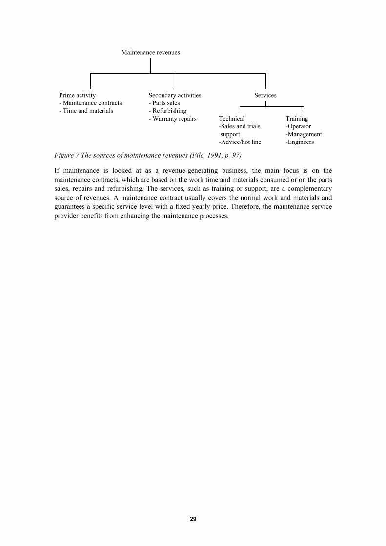
Maintenance revenues

ServicesPrime activity- Maintenance contracts- Time and materials

Technical-Sales and trials support-Advice/hot line

Training-Operator-Management-Engineers

Secondary activities- Parts sales- Refurbishing- Warranty repairs

Figure 7 The sources of maintenance revenues (File, 1991, p. 97)

If maintenance is looked at as a revenue-generating business, the main focus is on themaintenance contracts, which are based on the work time and materials consumed or on the partssales, repairs and refurbishing. The services, such as training or support, are a complementarysource of revenues. A maintenance contract usually covers the normal work and materials andguarantees a specific service level with a fixed yearly price. Therefore, the maintenance serviceprovider benefits from enhancing the maintenance processes.

30

5 SYSTEMS APPROACH TOMAINTENANCE

In this chapter, maintenance is approached from a systemic point of view. The assumption ofsystems approach is that there are many similar entities that behave similar way. Althoughfailure processes of machines are more or less stochastic, the systems approach seems to fitconceptually into modelling component behaviour in failure and maintenance processes.However, the systems approach is not a common one. Contrary, the modelling and optimisationof maintenance strategies are usually based on control of stochastic systems (e.g. Høyland andRausand, 1994) or on applying decision theory (e.g. Vatn et al., 1996; Vatn, 1997). The value ofsystems approach is in its capability to simplify complex problems and model the dependenciesin a system. The drawback is the possible oversimplification and the assumed determinism in themodels, which reduces the quantitative application of the models. However, in this research isthe interest is more on the behaviour than in the optimisation of maintenance systems.

5.1 SYSTEMS

The exact definition of a system varies by author (Kerr, 1991; Klir, 1985; Laszlo, 1972; Turbanand Aronson, 1998; Saaty and Kearns, 1985; Schoderbek et al., 1990; Weinberg, 1975).However, all definitions share a common idea of an interrelated set of functions and structuresthat serve a purpose.

According to Saaty and Kearns (1985), the purpose of a system is a behavioral concept anddifficult to define. They system purpose may change over time or it may have several levels,such as long-time goals, short time objectives and ideal system states to approach in order tosatisfy an objective. A man-made system serves the purpose of its designer or the system user.As an observer-related concept, a system may have several different interpretations, according tothe observer. A system can always be considered a subsystem of some larger system.

5.1.1 Functions, structures and environments

System functions transform purposes into action. These actions thus realise the purpose. Afunction can be described as an aggregate of its states in space and time. The functions may beoperating parallel and sequentially and the behaviour of the system functions affects thebehaviour of other functions. A system that is factored to its subsystems will consist of ahierarchical set of functions. The functions are carried out by flows. The types of flows can bematerial, energy, information, or transformations from one state to another state. Structure is aset of constraints on flows in space and time. It consists of forms or parts that relate to oneanother to perform a function (Saaty and Kearns, 1985).

An environment always surrounds a system, and the system is separated from itsenvironment by a boundary. The boundary can be physical, or time frame or some other limitingelement (Turban and Aronson, 1998). The interconnections and interaction among the systemsand their environment are called interfaces. The boundary between the system and itsenvironment is not always clear, but blurred. A system is called open if it is very dependent onits environment. Fully closed systems are more theoretical than real, because the only knownfully closed system is the universe. Closed systems do not need external energy or release energy

31

to their environment. They also tend to attain maximum entropy5. Open systems exchange inputand output flows with the environment, and may attain a time-independent steady state with thehelp of self-regulation.

5.1.2 Complexity and interdependencies

It is characteristic to systems that they are usually very complex, and the system componentshave a high number of strong internal connections. The complexity can be described with thenumber of interactions and interdependence (Saaty and Kearns, 1985) or the number of systemattributes (Schoderbek et al., 1990). The elements are interdependent and the intensity of thedependencies varies.

The interdependence is symbiotic, if the systems are dependent on each other for theirexistence. The system consisting of subsystems can have emergent properties. That is, suchproperties that cannot be found or understood in subsystems since they are generated oramplified by interaction between the subsystem functionalities. Such a relationship is also calledsynergetic (Kerr, 1991; Schoderbek et al., 1990). Weinberg (1975) states as a rule that the wholeis more than the sum of its parts, but also notes that the part is more than a fraction of the whole.The latter statement tries to remind that even if subsystems do not seem to have emergentproperties, the subsystem may be a part of some other system or have an emergent property therewhich is not observable in the currently observed system. That is, a subsystem may serve severalpurposes and several systems.

To survive, a system must be adaptive in regard to the changes within itself or in itsenvironment. The adaptation can occur either in the short run or in the long run. The forms ofadaptability are either functional or structural. Short-run adaptation takes place throughfunctional changes, whereas long-run adaptation occurs through structural changes. (Schoderbeket al., 1990). The adaptation can affect the internals or the environment of the system. In thelatter case, the possibilities to control the changes are much more restricted than in the formercase, because the system boundary restricts the possibilities to manipulate the environment.However, it may be possible to acquire environmental information, or information from insidethe system to help in adapting the system.

5.1.3 Factoring and integrating systems

The method to understand and possibly to find some rules and model the system is to dissect it tosmaller subsystems (Weinberg, 1975). To factor a system into subsystems Kerr (1991) suggestsrecursive top-down factoring to simpler systems that contain understandable processes. Theboundaries and interfaces should be clearly defined. In a perfectly connected system, where allthe subsystems are connected to each other, there are n⋅(n-1)/2 interconnections, where n is thenumber of subsystems. This makes any such system very difficult to control. Simplification ofthe interconnections is therefore essential. Kerr (1991) provides two approaches to simplifysubsystem interactions:

1. By forming clusters of subsystems that interact with each other by using a specialisedinterfacing system. The clusters interact by using the interfacing system. A division managerwho acts as a representative of his/her organisation can be regarded as an interfacing system

2. By decoupling subsystems to avoid interaction analysis. Decoupling can be done by usingbuffers, slack resources or standard procedures. Heylighen and Joslyn (2001) call thesemethods as passive mechanisms to dampen disturbances in a system.

5 Entropy here refers to statistical entropy, a measure of system variety defined by the possible states the system canbe in.

32

Inventory is an example of a buffer. It reduces or eliminates randomness in a production chain topropagate backward or forward, and makes control of the systems easier. Slack resources arecapacity that is not used until the normal capacity is unavailable, e.g. a stand-by equipment orpersonnel. Standard procedures aim at standardising the informational inputs and outputs of asystem to eliminate the sources of ambiguity and misunderstanding.

Sometimes it is feasible to integrate systems, i.e. when clustering systems instead ofdecoupling them. Miller, Rosenthal and Vollman (1986) have defined three types of integrationin manufacturing environments. Technical integration involves establishing physical connectionsbetween the functional areas. Procedural integration uses common data and has a consistentinterpretation of that data between the functional areas. Goal integration uses the sameinformation to achieve common goals or an objective.

5.1.4 Control systems

To guide the system toward its goals there must be a control decision-making system thatcontrols the controlled element in the system. Classical cybernetics, which studies the controland communication of systems, recognises three paradigms of goal oriented system control:open-loop or information-less paradigm, feed-forward paradigm, and feed-back paradigm(Wiener, 1961). The difference is which source information the decision-making element uses:no source information, the same input information as for the controlled element, the outputinformation of the controlled element, or some combination of them (Klir, 1985, p. 366).

According to Ashby’s (1957, p. 206) Law of Requisite Variety, the larger the variety ofactions available to a control system, the larger the variety of external perturbations and internalstates it is able to compensate. The law states that only variety in the regulating system can forcedown variety due to the controlled system. The law has two implications (Umpleby, 2001):First, there must be a control system that equals the variety of the controlled system. Secondly,the amount of appropriate selection that a control system can perform is limited by the amountof information available about the controlled system. The law is a logical law applicable to agiven set of possible states and the actions on those states, not an empirical law that is derived byobserving a real system.

5.1.5 Maintenance activities as a system

There have not been many studies about maintenance as a system. Kerr (1991) briefly notes thatmaintenance can be divided into tactical planning of preventive maintenance and operationalcontrol of the execution of the maintenance itself. He suggests that the loss of capacity due toplanned and unplanned maintenance should be known for planning the maintenance, as well asthe complete history of the occurred failures and their frequencies.

It is also difficult to separate the production process and the maintenance processes. Theapproach Jonsson (1999) takes is not to separate maintenance from production, but to considermaintenance as a part of the production process, as shown in Figure 8. The maintenance in thismodel creates production capacity, which is secondary input for the production process, and theproduction creates maintenance need, which is secondary output of the production process.Jonsson's (1999) research results indicate that companies that integrate maintenance and theirproduction strategy have a better competitive position.

33

Primary Input Primary OutputProduction process

Maintenance

Secondary Input Secondary Output

Figure 8 The production and maintenance processes (Jonsson, 1999, p. 26).

Lee (2001) presents a more idealistic approach. His focus is on an overall machine optimisationand management system that is enabled by an intelligent machine. The system closes the loopbetween maintenance and the production as shown in Figure 9. The proposed system shouldinclude the machine model that includes the wear and degradation process, diagnostics and faultdetection algorithms. The actual equipment condition should be possible to measure or simulate.A maintenance model, including a supply chain and management model should exist. Themachine and the maintenance model should be refined according to the maintenance andequipment condition history. Also, a rough production process model should be included in thesystem to manage and simulate the relations of the production process to the equipment and themaintenance process.

IntelligentEquipment

Production

Maintenance

actual capability

estimatedcapability

Maintenanceaction

utilization

estimated equipment availability

estimated cost ofdowntime

Figure 9 An enterprise-wide smart machine optimisation and management system. Modifiedfrom Koç and Lee (2001).

5.1.6 Machine reliability and maintenance system effectiveness

Allen (2001) distinguishes the approaches to study the effect of maintenance into either physicalmachine health or maintenance system effectiveness itself. In the first approach, all those actionsare considered that reverse the effects of machine ageing over the component life-cycle. Thismakes it possible to clean the effect of maintenance to the machine. The drawback is that theevery single maintenance action should be tracked over the total life-cycle of a component in aconstant process environment.

34

In the latter approach, the machine age is calculated backward from the failure to themoment the machine was take into use or renewed. This approach does not take into accounteach maintenance task but the overall maintenance on the machine. Thus, any ad-hocmaintenance is considered as an external influence on the maintenance system. The question thatAllen (2001) raises is whether to model the reliability of the controlled system (reliabilityengineering) or model the effectiveness of the control system (RCM, TPM). The difference is inthe application of the information.

5.1.7 Summary

Maintenance can be considered as a control system for controlling the reliability of machines ina process environment. The variety of possible states is constrained by the maintenance actions.Preventive maintenance can be considered as feed-forward control and reactive maintenance asfeed-back control. Condition-based maintenance reacts to the signs of possible future failures,and is therefore is a mixture of reactive and preventive maintenance. Consequently, condition-based maintenance represents neither pure feed-forward nor pure feed-back control. If thepreventive maintenance schedule is changed according to the occurred failures, the maintenancesystem adapts its behaviour with a higher level of feed-back control.

Because machines are open systems exchanging materials, energy and information with theirenvironment, their control is complex and rather unpredictable. Ashby's (1957) Law of RequisiteVariety suggests that the more there is information about the machines the more possibilitiesthere are to select the appropriate maintenance action to control the reliability.

5.2 MAINTENANCE SYSTEM PERFORMANCEMETRICS

The objective of this research is to model maintenance systems and the effects of conditionmonitoring. The operation of a maintenance system must be measured to model the effects ofcondition monitoring and to be able to control the system. This chapter reviews some of themaintenance system metrics that could be used as the controlled variables.

5.2.1 Efficiency and effectiveness

Turban and Aronson (1998) propose that systems should be measured with both effectivenessand efficiency. They define effectiveness as the degree to which the goals are achieved.Effectiveness is concerned with the results and outputs of the system. Efficiency is a measure ofinputs to achieve outputs. In other words, effectiveness is about doing the right things, andefficiency is about doing the things right. Sharp and McDermott (2001) propose several processmetrics such as the number of times the process has been executed, the process cycle time, thecost per execution, cost of defects, and the ratio of good output versus bad output.

Johnstone and Ward (1981) describe metrics for the maintenance system measurement, suchas the number of personnel accidents, maintenance budget variance, maintenance cost permachine, maintenance cost as percent of capital investment or percent of machine uptime,workload backlog, overtime ratio and emergency work ratio of total work. Middleton andStevens (1999) define three business types: cost-constrained, capacity-constrained andrequirements-constrained. For each of these they suggests different primary metrics: costs, OEEand quality rate. Wireman (1998) describes several other metrics, including also those thatmeasure the usage of computerized maintenance systems. He also notes that a common mistake

35

in measuring efficiency is using only the input values of the maintenance process, such as thenumber of work orders completed and maintenance personnel as percentage of total personnel.

5.2.2 Overall Equipment Efficiency

Jonsson (1999) suggests that maintenance effectiveness should be primarily measured with theOEE metrics of TPM. According to Jonsson (1999), the strengths of OEE lie in its simplicity andsupporting quality management, continuous improvement and internal efficiency measurements.OEE calculation presented by Nakajima (1988) does not take planned downtime into account.The practice varies, and some authors calculate planned downtime in the OEE availability (e.g.Jonsson, 1999).

Bonal et al. (1996) suggest metrics that combine the OEE calculation and investment costs ofthe machines. The goal is to maxims the utilisation of the constraining bottleneck machine of aproduction line, i.e. the efficiency of the machine in respect to the investment costs. Otherwisethe productivity improvements could be lost because of production bottlenecks. Moubray (1997)claims OEE to be misleading focusing on achieving the maximum performance from a machineregardless of what the performance requirements are. In addition, he states that the costs ofquality losses, performance losses and availability losses are not financially comparable. Thecosts of scrap include raw materials plus the lost profits, whereas performance and availabilitylosses include only profits. Therefore the quality, availability and performance rates would notbe multiplicative.

5.2.3 Availability

By definition (IEC 60050-191, 1996) reliability is a measure of what the ability of a machine toperform a required function for a given time interval is. Availability is a measure of what theability of a machine to perform a required function at a given instant of time is. These terms havequantitative relationships (US Department of Defence, 1982; IEC 60050-191, 1996) as definedby the following inherent availability equation

MTTRMTTFMTTFAi +

= (2)

where MTTF denotes the mean operating time to failure, and MTTR denotes the mean time torestore or repair. MTTF is a measure of machine reliability and durability: the longer theoperating time between the failures the more reliable and durable the machine is. MTTR is ameasure of machine maintainability, which tells how much time it takes to restore a machine tothe working state in optimal conditions. Operational availability is defined by

MDTMTBMMTBMAo +

= (3)

where MTBM denotes the mean operating time between maintenance, and MDT denotes themean downtime caused by maintenance – or lack of maintenance. MTBM is a measure of theproactive and reactive maintenance frequency of the machine. MDT is a measure of how longtime the maintenance takes on average.

The difference between (2) and (3) are that inherent availability Ai is mainly affected by themachine design. The design affects the reliability (MTTF) and maintainability (MTTR) of amachine, which can be seen as the maximum in inherent availability of the machine. Operationalavailability Ao represents the availability of the machine in its operating context. Both MTBMand MDT of Ao calculation are affected not only by design, but also by spare parts availability,

36

the applied maintenance policy, and other operational constraints. NASA (1996, pp. 3/20-3/21)defines the availability metrics as follows:

Inherent Availability Ai(1) The probability that a system or equipment, when used under stated conditions in an idealsupport environment will operate satisfactorily at any point in time as required.(2) Excludes preventive or scheduled maintenance actions, logistics delay time andadministrative delay time.

Operational Availability Ao:(1) The probability that a system or equipment, when used under stated conditions in an actualoperational environment will operate satisfactorily when called upon.(2) Includes active maintenance time, logistics delay time and administrative delay time.

5.2.4 Proposed effectiveness and efficiency metrics

Turner (2002) criticises the informative value of MTTF. In his opinion, the MTTF is in practicedifficult to calculate. The MTTF information is usually not available by failure type orcomponent level, and the machine components may be replaced by maintenance and thereforehave an effect on the MTTF. In addition to these arguments Turner states that the maintenance ofthe machine, in fact, aims to prevent failures before they occur, and therefore MTTF and Ai

calculated for any machine in operation are unreliable. In other words, he sees the drawbacks inapplying MTTF in reliability modelling (see Chapter 5.1.6). For similar reasons, the USDepartment of Defence (1982) suggests that the inherent availability Ai should be used only infactory acceptance tests, not in measuring the operational reliability of machines.

However, MTTF can be used in maintenance system effectiveness measurement. This isbecause in reliability engineering the effect of maintenance must be cleaned from the MTTFcalculation, but in measuring maintenance system the effect of maintenance must be included inthe metrics. The MTTF reveals the effectiveness of the maintenance programme in a certainoperating context for a machine under it, and therefore enables control of the maintenancesystem. Therefore, in this dissertation it is proposed that MTTF can and should be used as themaintenance system effectiveness metrics.

Machine reliability is affected also by other factors than maintenance, such as machinedesign. Therefore, high reliability is not absolutely achieved by effective maintenance unless theother affecting factors make high reliability possible.

Successful control of a maintenance system requires measurement of both the system outputs(effectiveness) and inputs (resources). The operational availability equation (3) and somevariants of the OEE equation (1) include the proactive maintenance downtime factor, but theother required input resources, such as materials or labour costs of the maintenance system, arenot included in the metrics. Consequently, this results into a single objective to take as muchcapacity out of the machines as possible in regard to calendar time. Therefore, the usage of suchmetrics in maintenance system control yields optimal results only temporarily, e.g. when there isnot enough production capacity.

Efficiency is defined in this research as a measure of the ability to use the available resourcesto generate the required output. Efficiency can be measured by the required input resources, suchas time and money used in the maintenance system with regard to the reliability that themaintenance system generates. Reliability has an effect to the number of failures and amount ofdowntime and therefore the proposed efficiency metrics is the cost of maintenance and failures.In practice, the costs must be normalised. For example, the cost of human injuries andenvironmental hazards should be normalised so that they can be compared to direct and indirectmonetary losses.

37

5.2.5 Availability of source data for the metrics

In the real life, there is a problem of how to collect the information to calculate the metrics.There are numerous mathematical models in reliability engineering that can be used inestimating machine lifetime, the effect of maintenance on machine reliability and much more. Asmathematical models they are valid, but real-life calculations with these models face the problemof definitions and accuracy of the source data. The definitions and the accuracy of measuringsuch quantitative maintenance system metrics as the number of failures, operating time anddowntime vary by paradigm, observer, available number of samples and data collection methods.Therefore, a mathematical reliability engineering method will yield results that are comparableonly to results of similar reliability paradigms, definitions and data collection methods. Thus,MTTF, OEE, or Ao of a machine cannot be compared to the MTTF of other machine unless thedefinitions, reliability paradigms and data collection methods are similar.

In practice, there seems to be no easy way to gather and calculate accurate operationinformation from machines, especially the uptime and stand-by time information. Several papersin a Finnish national technology programme report (TEKES, 2001) pinpoint difficulties orsuggest automated data collection methods for acquiring the availability data (Foster WheelerEnergy, p. 22; Konola, p. 36; Mäkitalo, p. 54; Välisalo, p. 67). The methods in the report mainlyutilise data from the production and maintenance personnel by using special reporting systems orthe reports in the maintenance systems. Depending on the organisation, industry, plant policies,technology, culture, and maintenance process the source data was gathered and the results wereachieved in different ways, case by case, machine type by machine type.

5.3 FAILURES

What seems to be differing in the various reliability paradigms and methodologies is thedefinition of basic maintenance terms. The semantics of words is not exactly the same in thedifferent approaches to reliability. If the definition of a single word that separates a fullyworking machine from a non-working one is weak, how is it possible to know when amaintenance action is needed? Even standards have contradictions: IEC 60050-191 (1996)defines failure as an event, whereas SAE J1011 (1999) defines failure as a state.

5.3.1 Failure states

The systems theory suggests that a system function is defined by its states and the state changes.This is in parallel with RCM and TPM thinking, where the failures are system states. Therefore,it is assumed that a failure is a state. I.e., failure state Sf ∈ S, where S = {S0, S1, …, Sn} is a set ofpossible system states.

The systems approach argues that any system state is observer-specific (Ashby, 1957;Weinberg, 1975). That is, for observers A and B the failure states Sfa ∈ S and Sfb ∈ S may differso that Sfa≠Sfb. This does not state that the objectivity of observations is a sufficient condition forobjective failure definition, but it helps in understanding why possible system states should bemodelled. It also helps in understanding the RCM/FMEA approach in which the possible failurestates are explicitly defined. Only if the failure state is explicitly defined, can the failure state beobjectively observed and proactive control actions planned. However, the state definition, e.g.that temperatures of over 50 degrees mean failure, still remains subjective.

In practice, a production system is a man-made system with a purpose. Therefore, the failurestate is always defined by a user. A production system may have several users, or stakeholders,having different viewpoints and attitudes concerning the purpose of the system. Therefore, the

38

user is merely a role of an organisation, and the failure definitions are not necessary person-specific but role-specific.

5.3.2 Failure patterns

RCM-related studies (Moubray, 1997; Allen, 2001; Turner, 2002) suggest that increasing thenumber of maintenance tasks does not necessary increase the reliability of a machine. Thestudies show that in the aircraft and marine industries most of the failures occur because ofcomponents that do not show any ageing but only infant mortality and constant failureprobability after that. The more maintenance and replacements of these components are done,the more unreliable the systems become.

Figure 10 shows six generic failure patterns of components during their life. A notablecharacteristic is that only 8-29 % of failures are age-related in such a way that the failure rateincreases with age. The rest of the failure rates are constantly random or present infant mortality,which results in that no scheduled restoration can improve the reliability of the component.

UAL Broberg MSP SUBMEPP1968 1973 1982 2001

4% 3% 3% 2%

2% 1% 17% 10%

5% 4% 3% 17%

7% 11% 6% 9%

14% 15% 42% 56%

68% 66% 29% 6%

Figure 10 Four studies of failure rates as functions of component ages referred by Allen (2001).UAL and Broberg were studies about aeroplanes, MSP about ships, and SUBMEPP aboutmilitary submarines.

Figure 10 shows that the frequency of occurrence of the failure patterns is highly specific tocontext and the observation method. Both Allen (2001) and Moubray (1997) note that the first“bathtub” curve is a result of a combination of other failure patterns, consisting of failure eventsof infant age, a period of random failures and sudden wear-out. Allen (2001) also suggests thatthe third, constantly increasing failure pattern may also be a combination of multiple suddenwear-out failure events of the second type. Generally speaking the more components in a system,the more types of failure events it will have. If the system is thoroughly tested and run in afterinstallation, the design and installation errors are not shown and there are less 6th type infantmortality failures.

39

5.3.3 Failure causes and effects

There is also a difficulty in differentiating the failure cause and effect. A manufacturing system,whether a machine or a production line, usually comprises several components. Each componenthas a certain inherent reliability and is exposed to external or internal failure events. Thesecomponents form a reliability network that defines the total reliability of the system. There maybe an almost infinite number of dynamic, static, operational, logistical, electrical, mechanicaland chemical connections that define the interdependencies of the network. The failure event ofone component may cause failure effects that look as failure events to other components. Thefailure event may therefore propagate through the system causing a flow of failures for thefollowing components. E.g. a wear-out of an air compressor filter causes dirt to block apneumatic actuator which stops a production line.

The two failure events are dependent if and only if P[E1·E2] ≠ P[E1] x P[E2] (Villemeur,1992). That is, if the joint probability of two failure events does not equal the product ofindividual probabilities of the events. According to Villemeur (1992) the categories of dependentfailure events are common cause events that have the same direct cause, and events that createintersystem or intercomponent dependencies such as a failure of a redundant component. Thecommon cause event types can be divided into design, construction, operating and maintenanceprocedures or environmental effects. Villemeur (1992) refers to several nuclear and aviationfailure databases indicating that the common cause failure events comprise 4-9 % of all thefailure events. Design errors are the most dominant (40-50 %) among the common cause failureevent types, followed by operating errors (30-45 %) and manufacturing and assembly errors (10%).

The division of dependent or independent failures is highly specific to context and theobservation method. Generally speaking, a failure event that seems to be random is notnecessarily random, but may just be out of the methodological or observational accuracy.Therefore, any comparison or judgement about failures or their causes should be very careful.

5.3.4 Partial failures

The concept of partial failures is well acknowledged by RCM, TPM and control engineering, butnot often noticed in reliability engineering. Partial failures are usually considered as performancedegradation or deterioration, and therefore modelled mathematically as continuous dynamicalsystems, which is not in the field of study in reliability engineering. Instead, Markov chains(Bukowski and Goble, 2001; Endrenyi et al., 2001; Wiseman, 1999) and lately also Petri Nets(Schneeweiss, 2001), have been used to model the development and probability of occurrencesof system states.

Endrenyi et al. (2001) present a simple Markov chain-based model between the random totalfailures, deterioration (partial) failures and proactive maintenance with two figures presented inFigure 11. A simplification of continuous deterioration with intermediate discrete states makesthe failure process easier to model. There are two ways of defining the intermediate states: eitherby operating time, which is an approximation of the real state, or physical signs, which requiresperiodic inspections or continuous condition monitoring.

40

FW S2S1 S3 S4

M M1 M2 M3

Figure 11 State diagrams for total and partial failures (Endrenyi et al., 2001) W:working state;F:failed state; S:state; M:maintenance state.

The problem in this kind of a presentation is in deciding in which of states S1-S4 the machine isconsidered failed. In the RCM approach the user may decide that S3 is a failed state. In reliabilityengineering S4 is considered definitely a failed state and S1 definitely a working state. In TPM itis agreed as in RCM that S3 may be a failed state, but the aim is to remain in state S1.

5.3.5 Subjective state definitions in the maintenance paradigms

In practice, there must be several organisations and paradigmatic approaches involved with aproduction system. Emergency repairing, predictive maintenance, preventive maintenance,system optimisation and operational system control all try to control the system states. Theallowable and satisfactory system states, however, differ in the various paradigms. Figure 12tries to capture the paradigmatic approaches to the control of system states.

State Variable

State Variable

Total Failure RegionAbsolute definition

Partial Failure RegionDefined by individual user requirements

Normal Operation RegionDefined by average capability

of this machine

Best Possible RegionDefined by best known machine

CE

RCM

RE

Designed Operation RegionDefined by machine & process designerTPM

System Dynamics

Figure 12 Paradigmatic approaches to the control of system states. TPM tries to move theoperating state to optimal region, control engineering tries keep the status quo, RCM tries tokeep the operating state away from failure region, and reliability engineering tries to keep thedesigned operating state. A total failure, meaning the total loss of a function, is the only commonfailure state for all the paradigms. The solid arrows describe the system control approachesemphasised by each paradigm and the dashed arrow is a system- dependent drift. In reality,there may be more than two states defining the system state.

41

5.4 EFFECTS OF INFORMATION IN FAILURE ANDMAINTENANCE PROCESSES

It was stated earlier that the number of appropriate maintenance action types the maintenancesystem is able to use is limited by the information available of the machines under maintenance.The statement is discussed in this chapter.

5.4.1 The observability and reversibility of black-box system states

Imagine that the machine or production line state is not observed other than after the actualfailure occurrences. Proactive control, i.e. preventive maintenance, would require a model of thesystem failures.

If the internal states of the system are not known, the system can be modelled as a black box,that has only two states. In that case, nothing needs to be known about the system internals. Thesystem seems to exhibit time-dependent behaviour or behaviour dependent on some otherexternal variable of the binary state changes, and can therefore be modelled with the help ofstochastic models. An example is the reliability engineering approach in which a machine iseither failed or not failed. A common approach to model such failures is to take the operatingtime as the independent variable, and the failure rate as the dependent variable. The failurepatterns shown in Figure 10 are based on such models.

If the failures are binary states, then the application of a stochastic failure model forpreventive maintenance requires that a maintenance action restores the failure totally or to somedefinite pre-failure state. In other words, the maintenance action can return the system only tothe beginning of the hazard curve or to some definite point along that curve as illustrated inFigure 13. This reduces the number of appropriate maintenance action types, and suggests a totalrestoration of the system.

Failure

Repair

Preventive Maintenance

Figure 13 In black-box systems it is assumed that maintenance always returns the system to thehazard curve and that the form of the curve does not change due to maintenance.

The challenge in complex systems is that if the sub-systems are renewed separately, the wholesystem will not be in the same state after the maintenance as it was before maintenance and themodel cannot be used in preventive maintenance programming. Therefore, the systems should bedivided into subsystems and the subsystems should be modelled separately.

5.4.2 Condition monitoring

If the system is monitored with a condition monitoring system, the system becomes a white or agrey box system. In that case, the condition monitoring method restricts the variety of possible

42

observable system states. The knowledge of which monitored system states are consideredfailure states must exist in order to prevent the system from failing. The control engineeringparadigm assumes that a given system state should be maintained and therefore uses no explicitdefinition of each failure state, but an explicit definition of the preferable operating state.Consequently, the explicit definition of the preferable operating state excludes all the other statesand therefore becomes an explicit definition of one failure state.

According to Shannon (1948) by acquiring enough information even over a noisytransmission channel it should be possible to obtain accurate information of a system state, andtherefore control the variety in the system states with the help of a given model. A system, inwhich the system states are stochastic and the observations take place trough a stochastic processas well, could be estimated by modelling the system with some advanced system identificationmethods, such as hidden Markov models (Rabiner, 1989), proportional hazards models(Wiseman, 1999) or stochastic filtering such as Kalman filters (Drécourt, 2003). Even though thehuman brain does not operate similarly to computers, there is no doubt that a human brain canalso create similar system models unconsciously. Therefore, an experienced mechanic may knowquite accurately when the machine is going to fail based only on the machine age or human-sensible parameters. On the other hand, a human error may affect the observation of the states.To rely on human perception as an observation channel increases the risk that a person does notrecognise the system state or reports the observed system state subjectively. If the conditionmonitoring is automated, the human transmission errors are reduced. Therefore, automaticcondition monitoring should help in developing better proactive maintenance programsregardless of the applied modelling method.

The increased number of monitored system states makes it possible to apply a wider range ofmaintenance actions than in an unobserved system. This is because the maintenance actions maychange the system state to a wider range of states, and the condition monitoring makes itpossible to know the exact state of the system. In practice, the human senses are such conditionmonitoring systems. Therefore, more maintenance actions than in a theoretical unobservedsystem should be expected in a real maintenance system. If electronic condition monitoringmethods that are able to sense system states beyond the human senses are applied, the number ofpossible maintenance actions could be even wider than without electronic condition monitoringmethods.

Bukowski and Goble (2001) have defined a term diagnostics coverage to describe theprobability that a failure state can be recognised by a diagnostic system. Thus, any conditionmonitoring method should be able to increase the diagnostic coverage. Because conditionmonitoring increases the amount of information about the machines, there are more possibilitiesto choose the right moment to undertake the correct maintenance action. Any misinformation,false diagnostics or measurement inaccuracy reduces the possibility to select the correct timingand type of maintenance action. In a perfect condition monitoring system the all the states areobserved correctly.

For the purposes of this dissertation term observability6 is defined as the conditionalprobability that a machine state is observed correctly. I.e., P(o=s|s), where s ∈ S = {S0, S1, …,Sn} is the true state and o ∈ S is the observed state. In a perfect condition monitoring system theconditional probability P(o=s|s)=1,∀ s.

The assumption is that the data provided by the condition monitoring system is used as aninput for the maintenance system. A condition monitoring system without usage is worthless.

6 Note that the definition of observability differs from the mathematical definition (Wolovich, 2000) in mathematicalcontrol theory.

43

5.4.3 Condition-based maintenance actions

Condition monitoring does not facilitate the system modelling. The level of modellinggranularity can be much finer in systems under condition monitoring than without conditionmonitoring.The question is why model a system if it is under condition monitoring? The answer is thatcondition-based maintenance reacts to possible failures and prevents them from happening. Thepreventive part of condition-based maintenance needs a model of the failure process. If thecondition monitoring is perfect and the failure prediction can be done early enough, then themaintenance system is able to prevent all the failures. I.e, the failure states are avoided (MTTF =∞) only when P(o=s|s)=1,∀ s, and when tf>ti, where ti is the initiation delay of the maintenanceaction and tf is the shortest transition time between any working system state and any failurestate in S.

Under these conditions any maintenance action that reduces the variety or constrains thesystem state from being in the failure state would be enough. But to know when and how toact, the effects of both the maintenance actions and the failure processes on the system statetransitions should be modelled, implicitly or explicitly.

If the condition monitoring is not perfect then the system may enter in an unknown systemstate as a result of variability in the maintenance actions. Furthermore, if not using conditionmonitoring, a repeatable maintenance action is the only possibility to know the system state formodelling failure transition time. In that case, it is even more important that the maintenanceaction is repeatable and always results in a known system state. I.e. let M = (M0, …, Mn) and X= (X0, …, Xn) be pairs of maintenance actions and the resulting system states X0…n ∈ S. In casewhere P(o=s|s)=0 the system state is known after maintenance only if conditional probabilityP(Xj|Mj)=1, ∀ j=0, …,n. That is, perfectly repeatable maintenance is needed to "reset" thesystem to a known state in order to model the system transitions.

In practise, when using condition monitoring the observability P(o=s|s) is between ]0,1[.Therefore, observability, maintenance action initiation time and repeatability affect themaintenance effectiveness, i.e. MTTF.

5.4.4 Information creation in failure and maintenance processes

Failure and maintenance processes are information processes. That is, the processes change theinput information into output information. The failure and maintenance processes are irreversiblein regard to information. A failure process loses information of the cause of the failure, and amaintenance process loses information of the failure state. Generally speaking, it is not usuallypossible to detect the input information by observing the output information of the informationprocess.

However, according to Losee (1998) the irreversible processes also produce informationabout the process itself. That is, a human being may be able to model the process and therequired input information. By observing the failure states after failures and the operating statesafter maintenance it is possible to get information about the behaviour of those processes. Ifpossible, the input information of the processes should be available, to help understand theprocesses. E.g. it is useful to have failure reports before executing a maintenance action, and pre-failure system status reports after failures to get information about the failure and maintenanceprocesses. It is also possible to estimate the possible outputs with the given inputs if there is afinite set of possible processes. That is, with a detected system state it may be possible to predictthe failure state. The existence and behaviour of the processes may be difficult to estimate, andtherefore an experienced human is needed to create the scenarios.

44

To explicitly define the failure states and to develop a proactive maintenance strategy it ispossible to begin from the existing maintenance actions, as in PM Optimization, from theoccurred failure states, as in TPM, or from the scenarios of possible failure states, as in RCM.The information creation processes in the maintenance paradigms are different from each other.

45

6 SYSTEM MODELS I-V

Maintenance systems appear to be very difficult to describe in written text. In this chapter, themaintenance systems are therefore modelled with several methods in order to capture thecomplexity and various views to the maintenance systems.

6.1 OVERVIEW OF SYSTEM MODELS I-V

Five models were developed during the research. Two of them are qualitative models describingthe relations of the entities and activities in the system. Three of the models are quantitative formodelling the stochastic and dynamic behaviour of the maintenance systems. The overview ofthe models is presented below.

Model I Knowledge modelA unified modelling language (UML) domain model of failure andmaintenance concepts for sharing the knowledge constructsdeveloped in the literature study and theory part of thisdissertation.

Model II Control activities modelAn applied Gorry-Morton framework (Gorry and Morton, 1989)for understanding the decision making and control activities inmaintenance systems.

Model III Stochastic maintenance system model A stochastic simulation model for studying the effect of condition

monitoring on the availability and total costs of maintenance.Model IV Dynamic maintenance system model

A dynamic simulation model for studying the effect of conditionmonitoring and the maintenance quality on the reliability andmaintenance worker allocation.

Model V Dynamic supply chain modelA dynamic simulation model for studying the effect of remotecondition monitoring information feedback on the spare partssupply chain.

6.2 SYSTEM MODEL I: A UML DOMAIN MODEL OFFAILURE AND MAINTENANCE CONCEPTS

6.2.1 Purpose of the model

The primary purpose of the model is to share the knowledge acquired during the research. Thesecondary purpose is to develop a high-level conceptual domain model for future informationsystem development projects.

46

6.2.2 Knowledge, ontology and information communication

To develop a knowledge model, a definition for knowledge should be stated. Kerr (1991, p. 65)describes the knowledge about an environment or domain “as the set of organised constructspossessed by an individual at any particular time in relation to a particular environment ordomain”. Any new data that modifies the knowledge structures of the recipient is regarded asinformation. The knowledge is communicated between individuals by using messages thatconvey abstract symbols with some syntax. The recipient can convert the symbols to knowledgeonly by understanding the message syntax and by interpreting the symbols against an existing setof mental constructs. An identical set of constructs, a shared context, is required between thesender and the receiver to fully transfer knowledge. Two persons cannot have a fully identicalset of mental constructs, which makes full knowledge transfer impossible.

However, an explicit knowledge representation with the help of text or images may help inimproving the context sharing and therefore the communication of the information. Also,subjective activities, such as failure diagnostics cannot be automated if the mental constructs ofthe human decision making have not been modelled.

6.2.3 UML as a knowledge modelling methodology

From the point of view of information systems development this dissertation can be regarded asan analysis of maintenance activities. Analysis is the first phase in information systemdevelopment. As an activity, the analysis consists of investigation of the problem and therequirements. The difference between the analysis and the design is that the analysis does nottake into account how the system should be implemented but only what the system does. Thevalue of standard software engineering methodologies should be acknowledged in analysing theexisting information systems or in analysing the requirements for new information systems. Toserve the secondary purpose of the model, the knowledge should therefore be represented in aformat familiar to software engineering to enable its further usage in future information systemdevelopment projects.

A commonly used notation in software engineering is defined by UML. UML can beregarded as a knowledge representation format, as well as a software design notation. The use ofUML in the analysis makes it possible to use unified process (UP) (Larman, 2002) as a softwaredevelopment method. The dissertation research methodology does not enable the application ofthe unified process as such. Instead, one of the central concepts was picked from the unifiedprocess: the domain model.

The domain model is a description of things of interest in the real world and consists of a setof conceptual classes, their associations and attributes modelled with UML class diagrams.Larman (2002, p.129) defines domain models as “a visual dictionary of the noteworthyabstractions, domain vocabulary, and information content of the domain.” Comparing to theknowledge definition in Chapter 6.2.2 the domain model represents a knowledge model. Theclasses in the domain models show real-world concepts. The domain model is an analyst’s viewof the domain, and it should be distinguished from the design view of the software classes.However, the domain model can be used in designing the software classes of theimplementation. Therefore, the domain model communicates information about the domain andreduces the representational gap between the software implementation and the mental domainconcepts of the analyst.

6.2.4 Validation of the UML model with a knowledge modelling tool

The UML domain model has one major drawback in domain modelling: No class instances canbe defined. That is, an instance such as "oil change" cannot be defined for a concept named

47

"maintenance action". This makes it difficult to assess the validity of the model. Therefore, theUML model was developed with the help of a special knowledge modelling tool (Protégé-2000v1.7 from Stanford University). After changing the model in the knowledge modelling tool andentering some sample class instances, the same changes were made to the UML model. Then theUML model was simplified, and the same changes were made in the knowledge modelling tool.This modelling methodology was surprisingly powerful. The knowledge modelling tool made itpossible to test the model with instance data, which helped in refining the model.

6.2.5 The UML domain model

The resulting UML domain model is presented in Figure 14.

48

Figure 14 A domain model of failure and maintenance concepts.

The central concept is the system. A system can be connected to and from zero or more systemsrepresenting the logical arrangements of the system. In other words, an engine may be connectedto an exhaust system. A system may have zero or more sub- and supersystems. That is, aproduction line may consist of machines, and the machine may be a part of several productionlines. Each system has at least one purpose, that is the reason for the existence of the system. Apurpose may be implemented by at least one system. E.g. the purpose to generate power can beimplemented by a combustion engine or a gas turbine. A system may fail to a fault (failure state)or due to a fault (failure event). An example screenshot of the system concept from theknowledge modelling tool is shown in Figure 15. The structure is identical to the UML domainmodel.

49

Figure 15 A realisation of the system concept as represented by the knowledge modelling tool.

A fault represents both failure states and failure events. When entering instances in theknowledge modelling tool the distinction between a failure state and failure event was so unclearthat the separation between them was very difficult. Instead, a less informative concept, namelyfault, was used. In other words, a fault is a possibility for or an existence of a failure event orstate. The idea that both state and event are kinds of faults is bit confusing. However, an eventrepresents a state change. Therefore, an event can be described with the resulting state or a statewith the event. It is just semantics to think with failure occurrences or existences. In the model, afault may cause zero or more consequent faults, or a fault may be caused by zero or more faults.Each fault may have zero or more consequences, and each consequence is caused by at least onefault. A consequence is applicable in at least one environment. E.g. a total loss of pulpproduction capacity is applicable only in the paper making process. In an applicationenvironment there may be several fault consequences. An example screenshot of the faultconcept from the knowledge modelling tool is shown in Figure 16.

50

Figure 16 A realisation of the fault concept as represented by the knowledge modelling tool.

A condition monitoring system strives to monitor at least one fault, and a fault can be monitoredby zero or more condition monitoring methods. A maintenance action reacts to or prevents atleast one fault. Each fault must be reacted or prevented by zero or more maintenance actions. Amaintenance action requires at least one resource. A resource can be either material, such asspare parts or tools, or the work skills of a worker. A resource must be required by at least onemaintenance action. Each maintenance action may have zero or more schedules. A schedule, e.g.once per year, schedules at least one maintenance action. An example screenshot of the workskill and schedule concepts from the knowledge modelling tool is shown in Figure 17.

51

Figure 17 A realisation of the work skill resource and schedule concepts as represented by theknowledge modelling tool.

The explicit definition of faults in the domain model refers to the RCM/FMEA thinking in whichthe failure consequences cannot be defined if the failure state is not defined. Contrary toRCM/FMEA the system is defined with a purpose rather than a function. However, a function ora set of functions is needed for achieving the purpose. As stated earlier, a fault can be a cause oran effect of other faults. The thinking here is aligned with the fault tree analysis (FTA) methoddefined in IEC 61025 (1990). In the knowledge modelling tool the user can begin from anysystem purpose or fault and create a fully compatible model to FMEA and FTA.

6.2.6 Summary

The presented knowledge model defines a structure for maintenance system models. Themodelling tool helps in creating a realisation of such a maintenance system model and ensuresthat the system is valid. If there are discrepancies between the model and the actual system,either one or the other is not valid. Therefore, the realised model should be modified accordingto reality or the reality can be analysed and corrected. By adding quantitative failure andmaintenance models and by connecting the tool to a CMMS it would be possible to create anefficient real-time maintenance planning tool.

6.3 SYSTEM MODEL II: A GORRY-MORTONINFORMATION SYSTEMS FRAMEWORK

6.3.1 Purpose of the model

The failure and maintenance processes are very complex and unpredictable despite the vastvariety of methodologies and paradigms that can be applied to control the processes. Theapplicability of information technology depends on how much human intelligence can be

52

replaced with artificial intelligence (AI) and what kind of requirements AI places on theavailability and quality of the information for making the necessary decisions.

The UML domain model presented in Chapter 6.2 presents the knowledge constructs ofmaintenance systems. The constructs, however, do not tell how the maintenance systems arecontrolled. The purpose of the model is to understand the complexity of decision making andcontrol activities in maintenance systems.

6.3.2 Artificial intelligence

Even though the scope of this research does not cover the implementation of informationsystems, some characteristics of intelligence should be defined in order to understand the controlpossibilities of maintenance systems.

According to Turban and Aronson (1998) artificial intelligence is concerned with two basicideas. Firstly, it involves understanding what intelligence is by studying the thinking processesof humans, and secondly, it deals with representing those processes in computers. The signs ofintelligence include learning and understanding, responding quickly to a new situation, usingreasoning in solving problems, making sense of contradictory messages and applying knowledgeto manipulate the environment. Kaplan (1984) has defined several important commercialadvantages of artificial intelligence over natural intelligence: AI is more permanent, offers easeof duplication, can be less expensive than natural intelligence, is consistent and thorough, can bedocumented, can execute certain tasks much more quickly than a human, and can performcertain tasks better than most humans. However, according to Kaplan (1984) natural intelligencehas several advantages over AI: Natural intelligence is creative, enables people to benefit fromand use sensory experience directly, and human reasoning makes use of a wide context ofexperiences and brings that to work on individual problems.

Natural intelligence enables people to recognise relationships between things, sense qualitiesand spot patterns to make relationship recognising possible. These are very difficult to programin AI. Kaplan's (1984) definitions suggest that the problems that an AI system can solve must bewell structured and repetitive. Complex and unstructured problems require human intelligence.

6.3.3 The Gorry-Morton framework

The most complete knowledge and system-control related information system model foundduring the literature study was a framework for management information systems of Gorry andMorton (1989). The framework shown in Table 3 is based on the problem classification intostructured and unstructured types, as well as the time-horizon of the decisions.

Operational Control Management Control(Tactical planning)

Strategic Planning

Structured • Accounts receivable• Order entry• Inventory control

• Budget analysis• Short-term

forecasting

• Tanker fleet mix• Warehouse and

factory location• Production

scheduling• Variance analysis –

overall budget• Mergers and

acquisitions

Unstructured • Cash managementPERT/COSTsystems

• Budget preparation• Sales and

production planning

• New productplanning

• R&D planningTable 3 Management information systems framework (Gorry and Morton, 1989).

A structured problem is one in which the intelligence, design and choice phases of the problemsolving are structured. In other words, there are algorithms or decision rules that make it possible

53

to find the problem, design the solution alternatives, and select the best solution. Operationalcontrol systems include repetitive and pre-programmed actions that deal with accurate, internaland current or historical data, whereas strategic planning is long-range, infrequent, predictiveand uses mainly aggregated and external data. Typical corporate information systems reside onthe upper left corner of the framework. The information systems that deal with unstructuredproblems are usually decision support systems.

The main problem in implementing an information system in structured operational areas isto adapt the existing model to the organisation. Information system design in the unstructuredareas is more involved with the structuration and modelling of the problem and the problemsolving process rather than the implementation problem. The modelling and structuring of theunstructured problems make it possible to automatically or semiautomatically solve problemsthat would otherwise require a human expert. Gorry and Morton (1989) emphasise theimportance of understanding the critical decisions made by the organisation in order to createinformation systems that deal with unstructured problems.

According to Schoderbek et al. (1990, p. 118) "decision making and control are similar, ifnot identical managerial activities. Both activities are initiated and maintained throughcommunication." This statement suggests that the entire framework of Gorry and Morton isessentially a control system framework with regard to the control time horizon of the system andthe degree of structure of the control decisions.

6.3.4 Applying the Gorry-Morton framework to maintenance systems

According to the literature study, the framework of Gorry and Morton (1989) has not beenapplied to maintenance systems. Therefore, maintenance-related concepts and methodologieswere placed in the framework in order to analyse both the time frame and control decisioncomplexity of the system. Inspired by the version of the original framework Turban and Aronson(1998) present in their book, an additional column named "applicable methods" that describeswhat kind of methods exist to make decisions or to help make them in maintenance systems wasadded. The resulting framework with transitions from reactive to preventive maintenance, andfrom preventive to condition-based maintenance is presented in Table 4.

54

OperationalControl

Tactical planning StrategicPlanning

ApplicableMethods

Structured • Work orderentry

• Cost reporting• Condition

monitoring

• Maintenancedirect costsbudgeting

• Inventory andworkforceplanning

• Quantitativemodels

• Analyticalmodels

• Operationsresearch

Semistructured • Maintenanceworkflowcontrol

• Inventorycontrol

• Root causeanalysis

• Preventivemaintenanceworkscheduling

• Fault treeanalysis

• Maintenancework planning

• Failureeffects andconsequenceanalysis

• Run-to-failure or usepreventivemaintenance

• Descriptivemodels

• Process andevent models

Unstructured • Failurediagnostics

• Machine repair

• Failureprognostics

• Failure modeanalysis

• Long-termmaintenanceplanning

• Heuristics• Decision

supportsystems

• Expertsystems

• Neuralnetworks

Table 4 A maintenance information system framework and the transitions from reactive (lower-left circle) to preventive maintenance (middle-right circle), and from preventive to condition-based maintenance (upper-left circle).

By analysing the framework it is obvious that CMMS functionality lies on the operational-tactical timescale dealing mostly with structured-semistructured issues. Condition monitoring isalso a structured activity in the operations control, because it is frequently repeated and focuseson the current state of the system. Preventive maintenance is semi- or unstructured and affectsfuture system states in the medium or long-range time horizon. Therefore, when operating withstructured and current information, condition monitoring may enable more accurate maintenanceactivities than preventive maintenance. However, the diagnostics and prognostics of the failuresstill remain on the unstructured level implying that human intelligence is needed in decidingwhat kind of actions a detected system state requires.

RCM and TPM seem to be paradigms that deal with semistructured and unstructuredproblems in the failure-maintenance system, whereas reliability engineering and controlengineering are structured approaches. Therefore, a mix of the methods and paradigms in real-world maintenance is necessary. Without applying several different methods and paradigms thecontrol of the system would be difficult because of the missing decision making methodologies.Ashby’s (1957) statement that only variety in the regulating system can force down variety dueto the controlled system applies in the failure and maintenance processes. This also implies thatthere is no "silver bullet", e.g. a paradigm, policy or methodology, that would solve all theproblems related to maintenance systems.

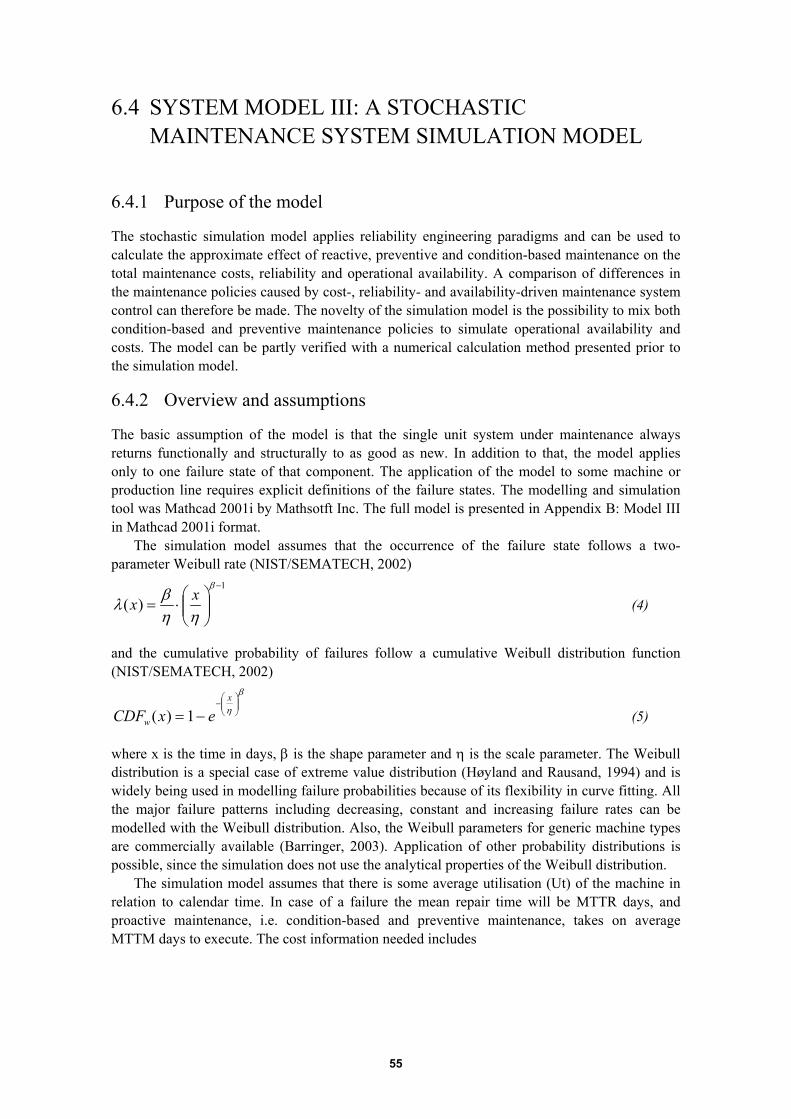
55

6.4 SYSTEM MODEL III: A STOCHASTICMAINTENANCE SYSTEM SIMULATION MODEL

6.4.1 Purpose of the model

The stochastic simulation model applies reliability engineering paradigms and can be used tocalculate the approximate effect of reactive, preventive and condition-based maintenance on thetotal maintenance costs, reliability and operational availability. A comparison of differences inthe maintenance policies caused by cost-, reliability- and availability-driven maintenance systemcontrol can therefore be made. The novelty of the simulation model is the possibility to mix bothcondition-based and preventive maintenance policies to simulate operational availability andcosts. The model can be partly verified with a numerical calculation method presented prior tothe simulation model.

6.4.2 Overview and assumptions

The basic assumption of the model is that the single unit system under maintenance alwaysreturns functionally and structurally to as good as new. In addition to that, the model appliesonly to one failure state of that component. The application of the model to some machine orproduction line requires explicit definitions of the failure states. The modelling and simulationtool was Mathcad 2001i by Mathsotft Inc. The full model is presented in Appendix B: Model IIIin Mathcad 2001i format.

The simulation model assumes that the occurrence of the failure state follows a two-parameter Weibull rate (NIST/SEMATECH, 2002)

1

)(−

⋅=

β

ηηβλ xx (4)

and the cumulative probability of failures follow a cumulative Weibull distribution function(NIST/SEMATECH, 2002)

β

η

−

−=x

w exCDF 1)( (5)

where x is the time in days, β is the shape parameter and η is the scale parameter. The Weibulldistribution is a special case of extreme value distribution (Høyland and Rausand, 1994) and iswidely being used in modelling failure probabilities because of its flexibility in curve fitting. Allthe major failure patterns including decreasing, constant and increasing failure rates can bemodelled with the Weibull distribution. Also, the Weibull parameters for generic machine typesare commercially available (Barringer, 2003). Application of other probability distributions ispossible, since the simulation does not use the analytical properties of the Weibull distribution.

The simulation model assumes that there is some average utilisation (Ut) of the machine inrelation to calendar time. In case of a failure the mean repair time will be MTTR days, andproactive maintenance, i.e. condition-based and preventive maintenance, takes on averageMTTM days to execute. The cost information needed includes

56

• component price (cco)• repair work costs (cre)• proactive maintenance work costs (cma)• daily lost capacity expenses of proactive maintenance (cdcap)• daily increased operating expenses caused by a failure (cdop)• daily increased quality expenses caused by a failure (cdqu)• daily lost capacity expenses caused by a failure (cdcar)

Therefore, the long-run mean yearly total costs of maintenance is given by

( ) ( )[ ] mccMTTRcdcdcdnMTTMcdccmnfc corecarquopcapmaco ⋅++⋅+++⋅⋅++=),( (6)

where n is the number of proactive maintenance actions and m is the number of repairs during ayear.

6.4.3 Numerical method of a preventively maintained system

With a given maintenance interval MTBM in operation days and failure rate function (4) it ispossible to calculate both the number of failures and the number of preventive maintenanceactions. The model is suitable for verifying this particular simulation model, although a moreelegant solution for calculating the failure and maintenance frequencies can be derived from therenewal theory (Høyland and Rausand, 1994, p. 292).

The calculation assumes that the preventive maintenance action changes the failure rate tothe same level as a new system after each MTBM operating days. This is described by thefollowing cumulative distribution function (Virtanen and Hagmark, 2002) if a Weibulldistribution is applied:

∫−−=x

MdxMTBMxexMTBMCDF 0 )),(mod(1),( λ

(7)

where mod(x, MTBM) represents the modulo operator that takes the remainder on dividing x byMTBM. This results in a curve type shown in Figure 18.

0 5000 1 .104 1.5 .104 2 .1040

0.5

1

Time

Prob

abili

ty o

f fai

lure

CDFM MTBM t,( )

t

Figure 18 Cumulative failure probability of a preventively maintained Weibull system (7) withMTBM=2700, β=2.5, η=4167.

The mean time to failure (MTTF) needed in the calculation is given by numerically integratingthe reliability function from zero to infinity (Høyland and Rausand, 1994)

57

[ ]∫∞

−=0

),(1 dxxMTBMCDFMTTF M (8)

The MTTF value does not equal the MTTF of a machine but the MTTF of the function that maybe implemented by several machines replaced by preventive maintenance.

The probability that a failure is observed during the first MTBM interval isCDFM(MTBM, 1·MTBM)-CDFM(MTBM,0). The probability that a failure is observed duringthe 2nd MTMB interval is CDFM(MTBM,2·MTBM)-CDFM(MTBM, 1·MTBM) and so on. Bymultiplying the probabilities by the respective number of maintenance actions gives the expectedvalue for the number of preventive maintenance actions per failure (mf):

[ ]∑∞

=

⋅⋅−⋅+=0

),())1(,(i

MM iMTBMiMTBMCDFMTBMiMTBMCDFmf (9)

which can also be written as

mnmf = (10)

where n and m are the number of preventive and reactive maintenance actions during a year.The mean calendar time to reach the first repaired failure (MTTFR) is given by

MTTRUt

MTTFMTTMnMTTFR ++⋅= (11)

where Ut is the average machine utilization. The number of reactive maintenance actions, andtherefore the number of failures during a year is given by

MTTFRm 365= (12)

The group of the three previous equations (10, 11, 12) can be solved to calculate number ofreactive maintenance actions during a year:

MTTMmf

MTTMmfMTTRUt

MTTFMTTRUt

MTTF

m⋅⋅

⋅⋅⋅+

++

+−

=2

36542

(13)

With m it is easy to calculate the n with the help of (10), and the yearly costs of maintenancewith (6). For analysis purposes also the operational availability is defined according to Chapter5.2.3:

365)(365 MTTMnMTTRmAo

⋅+⋅−= (14)

It is assumed that the production process is operating 24 hours per day and 7 days per week. Ifnot, then the MTTR and MTTM as well as the number of production days, 365, should beadjusted according to the production schedule. No method for calculating OEE is presentedbecause the quality and capacity losses are calculated directly with the cost function.

The numerical calculation method presented in this chapter is suitable to reactive-preventivemaintenance, but the effect of condition monitoring is difficult to implement in the presentedequations. Also, the numerical calculation of integrals and sums is quite slow. Therefore, themethod presented in this chapter was used only to verify the simulation results of the simulationmodel presented in the next chapter.

58

6.4.4 Simulation model of a preventively maintained system undercondition monitoring

Usually, condition monitoring is assumed to be able to detect the failure state 100 % reliably (i.e.Dieulle et al., 2001; Maillart and Pollock, 2002) or the condition monitoring reliability isassumed time-invariant (Bukowski and Goble, 2001). Also, condition-based maintenance isusually assumed to replace preventive maintenance as the maintenance policy. In reality theseassumptions are not always valid. For example, paper roll bearings are sometimes replaced evenif they are under condition monitoring. This implies either that the condition monitoring methodis not fully reliable or that the condition monitoring detects the failure too late.

In the simulation model, condition monitoring is assumed to be able to detect the futurefailure state with some certainty (DC) [0 % ...100 %], which is called diagnostic coverage(Bukowski and Goble, 2001). If the failure is detected, the detection time (DT) is the timebetween the found indication of a future failure state and the actual occurrence of the failure.

In reality, there is likely to be some dependence between DT and DC. That is, the meandetection time is longer with higher diagnostics coverage, and vice versa. But, because it may bepossible to adjust the sensitivity of the diagnostics there may be an increasing number of falsediagnostics alarms if DC and DT are increased. These aspects are not included in this model butconsidered later in Model IV.

In addition to cost parameters in the previous chapter, there is an additional cost of onecondition monitoring inspection (ci), and the monitoring interval parameter, mean operating timebetween inspections (MTBI). If using automatic condition monitoring as assumed in thisresearch, both ci and MTBI can be approximated as zeros. If applying the model in highlyintegrated process industries where a machine can be maintained only during some fixedmaintenance breaks, there must be some factor that defines what the average time is from thedetection of a failure to the next possible moment when the maintenance can be executedwithout interrupting the process. This time interval, mean operating time to arrange amaintenance break (MTTAM), may also be defined by the availability of suitable spare parts ormaintenance planning and scheduling delay.The simulation model uses two-parameter Gamma probability distribution

xexxPDF λαα

αλ −−

Γ Γ= 1

)()( (15)

where α is the scale parameter, λ is the rate parameter and Γ is the Gamma function to model theprobability of detecting the failure DT days before its occurrence. Use of other distributions ispossible, e.g. Beta distribution, which is very flexible and suitable for modeling expert estimateddata (Fente et al., 1999). In the simulation, the distribution is formed by user-given parametersfor mode (the peak value), median, 10 % and 90 % confidence levels for the detection times. Themode value is fixed as it is easiest to estimate (Fente et al., 1999). The least squares method isused to fit the Gamma distribution to the given points. An example of such distribution is givenin Figure 19.

59

0 20 40 60 80 1000

0.5

11

0

f_detection pdf x α, λ,( )

DT max 2⋅0 x

Figure 19 A Gamma probability distribution (15) with scale parameter α=2 and rate parameterλ=0.05 to model the failure detection time as a function of probability. The curve area on theright of the MTTAM line defines what the probability is that the failure is detected earlier thanthe time it takes to arrange maintenance (MTTAM=15 d).

An inverse of the cumulative Weibull failure distribution (5) as well as an inverse cumulativeGamma distribution are used in the simulation by feeding random probabilities between values 0and 1 to the functions. The functions return the simulated operating time to the next failure andthe detection time to detect the failure. The simulation proceeds as follows

1: take a random number between 0 and 1 and simulate the next failure time in operating days by using aninverse function of Equation 5 in respect to time x and sum it to previous failure or maintenance time2: determine the next preventive maintenance by adding mean operating time between failure (MTBM) toprevious failure or maintenance time3: if the simulated failure time is before the next preventive maintenance time, that is the system is goingto fail, then

4: take a random number between 0 and 15: if the random number is less than DC, that is, the diagnostics detect the failure, then

6: take a random number between 0 and 1 and use inverse cumulativeGamma distribution to simulate how many operating days before thefailure it is detected7: adjust the time of detection by selecting the next condition monitoringtime defined by the mean operating time between inspections (MTBI)from the previous failure or maintenance time8: if the failure time minus detection time is greater than the meancalendar time to arrange maintenance (MTTAM) then

9: the system fails at the failure time because themaintenance cannot be executed before the failure

else10: the predictive maintenance time is the detection timeplus MTTAM

else11: the system fails at the failure time because the diagnostics cannotdetect the failure

else12: the preventive maintenance is executed before the failure and the maintenance time isgiven by the previous failure or maintenance time plus MTBM

13: go back to step 1 until enough maintenance and failure events have been simulated

MTTAMMTTAMMTTAMMTTAMMTTAM

60

It is possible to count the number of proactive maintenance actions from the simulation resultsand apply (6) and (14) to calculate the average total costs of the maintenance and the averageoperational availability of the system.

6.4.5 Simulation results

To study the effect of condition monitoring a fictive electrical motor was used with Weibullfailure curve defined by β=2 and η= 4166.667 (Barringer, 2003) which analytically calculatinggives as the mean time to fail MTTF=3696.933 operating days. The preventive maintenanceinterval MTBM was set at 2700 operating days and the diagnostics coverage DC at 75 % of thefailures detected, if applied. Both the maintenance (MTTM) and repair (MTTR) take 5 calendardays. The cost information used was as follows:

• motor price cco=10,000• repair work costs cre=2,000• proactive maintenance work costs cma=1,000• daily lost capacity expenses in case of proactive maintenance cdcap=0• daily increased operating expenses caused by a failure cdop=0• daily increased quality expenses caused by a failure cdqu=0• daily lost capacity expenses caused by a failure cdcar=10,000

The proactive maintenance is not assumed to cause any capacity loss expenses (cdcap=0) tocontrast the differences between cost and availability-driven maintenance system control. Thecdcap would be significant only in a situation where the proactive maintenance would cause lossof sales. In case of repair or maintenance the motor is replaced with a renewed one. The repairwork is assumed more expensive than proactive maintenance because of the overtime workcosts. Proactive maintenance is assumed to be arranged immediately (MTTAM=0), so that thedetection time curve has no effect.

Four maintenance policies were studied: reactive only, preventive only, condition-based andpreventive, and condition-based only. The results are presented in Table 5 and Figure 20 with1,000,000 years of simulation.

Ao Costs / year MTTF (days) Failures / YearReactive 99.892 % 4892.0 3696.8 0.079Preventive 99.838 % 3023.7 8631.3 0.034Preventive & CBM 99.837 % 1735.4 34576.9 0.008CBM 99.891 % 1880.3 14770.5 0.020Table 5 Simulation results of four different maintenance policies.

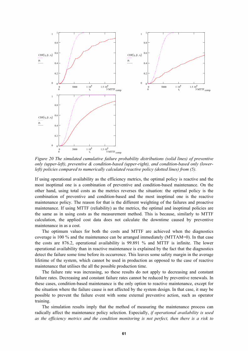
61

0 5000 1 .104 1.5 .1040

0.2

0.4

0.6

0.8

11

0

CDF ti β, η,( )pi

5 MTTF comp⋅0 ti0 5000 1 .104 1.5 .104

0

0.2

0.4

0.6

0.8

11

0

CDF ti β, η,( )pi

5 MTTF comp⋅0 ti

0 5000 1 .104 1.5 .1040

0.2

0.4

0.6

0.8

11

0

CDF ti β, η,( )pi

5 MTTF comp⋅0 ti

Figure 20 The simulated cumulative failure probability distributions (solid lines) of preventiveonly (upper-left), preventive & condition-based (upper-right), and condition-based only (lower-left) policies compared to numerically calculated reactive policy (dotted lines) from (5).

If using operational availability as the efficiency metrics, the optimal policy is reactive and themost inoptimal one is a combination of preventive and condition-based maintenance. On theother hand, using total costs as the metrics reverses the situation: the optimal policy is thecombination of preventive and condition-based and the most inoptimal one is the reactivemaintenance policy. The reason for that is the different weighting of the failures and proactivemaintenance. If using MTTF (reliability) as the metrics, the optimal and inoptimal policies arethe same as in using costs as the measurement method. This is because, similarly to MTTFcalculation, the applied cost data does not calculate the downtime caused by preventivemaintenance in as a cost.

The optimum values for both the costs and MTTF are achieved when the diagnosticscoverage is 100 % and the maintenance can be arranged immediately (MTTAM=0). In that casethe costs are 876.2, operational availability is 99.891 % and MTTF is infinite. The loweroperational availability than in reactive maintenance is explained by the fact that the diagnosticsdetect the failure some time before its occurrence. This leaves some safety margin in the averagelifetime of the system, which cannot be used in production as opposed to the case of reactivemaintenance that utilises the all the possible production time.

The failure rate was increasing, so these results do not apply to decreasing and constantfailure rates. Decreasing and constant failure rates cannot be reduced by preventive renewals. Inthese cases, condition-based maintenance is the only option to reactive maintenance, except forthe situation where the failure cause is not affected by the system design. In that case, it may bepossible to prevent the failure event with some external preventive action, such as operatortraining.

The simulation results imply that the method of measuring the maintenance process canradically affect the maintenance policy selection. Especially, if operational availability is usedas the efficiency metrics and the condition monitoring is not perfect, then there is a risk to

62

overvalue condition-based maintenance over preventive maintenance and reactive maintenanceover condition-based and preventive maintenance.

6.4.6 The effect of limited time to diagnose

If using 15 days as the mean operating time to arrange maintenance (MTTAM) and the detectiontime curve shown in Figure 19, the numerically calculated percentage for the components thatcould not be proactively maintained in time would be 17.3 % of the detected failing components.Therefore, with 75 % diagnostic coverage, 62.0 % of all the failures could be avoided. Thiscould be used as an approximation of diagnostics coverage with zero days MTTAM to getsimilar results.

In highly integrated process industries the MTTAM is defined by the scheduled maintenancebreaks. The production process cannot be stalled right away if condition monitoring indicatesfailure. In highly parallel production systems, such as cell production, there are no suchrestrictions. Therefore the MTTAM is merely defined by the spare parts availability and thethroughput time of the maintenance process workflow. In the previous example, dropping theMTTAM from 15 days to 10 days increases the percentage of avoided failures from 62 % to 68.2%.

Reduction of the maintenance process throughput time and condition monitoring have anamplifying effect on each other to increase reliability in situations where the maintenanceprocess cycle time limits arranging a maintenance break. However, the scale of the amplificationis dependent on the detection time, diagnostics coverage and the maintenance process throughputtime.

6.4.7 Summary

In the example simulation, the application of condition monitoring increased reliabilitycompared to the reactive and preventive maintenance policies. However, the condition-basedmaintenance with limited diagnostics coverage (observability) was not the optimal policy.

The presented model used only one failure type so the comparison between maintenanceactions was not done. However, if preventive replacement or renewal was the only maintenanceaction, adding additional failure types to the model would reduce the effectiveness of preventivemaintenance even more. This is because prevention of one failure type with renewal would bequite likely inoptimal in regard to other failure types.

The example simulation shows that the measurement metrics of maintenance system affectthe applied maintenance policy. Such metrics as operational availability seems to favourirrational maintenance policies that are usable only in special cases.

Because the detection time DT reduces the ability to do the maintenance action on thedetected failure in time, it is feasible to shorten the maintenance process throughput time withsuch technologies as computerised maintenance management systems in order to reduce theproduction losses in case of failures.

6.5 SYSTEM MODEL IV: A DYNAMIC MAINTENANCESYSTEM SIMULATION MODEL

6.5.1 Purpose of the model

The purpose of the model is to analyse the effect of the control system, condition monitoring,maintenance repeatability and worker resources to the dynamics of maintenance systems. Of the

63

presented models, this is dynamically the most complex one. The model is based on the theorypart and models derived so far. The dynamics cannot be predicted from the equations that definethe model structure, and therefore the model helps in revealing the behaviour of maintenancesystems.

6.5.2 Dynamic modelling

Dynamic models have their roots in system thinking and system control with informationfeedback. The origins of the applied modelling method are in the classic Forrester (1961) book.The modelling method emphasises studying the effect of the system structure and decisions onthe behaviour of the system. The three basic modelling elements are levels that describe the stateof the system, rates of flows that connect the levels and decision functions that control the rates.Levels accumulate the incoming and outgoing rates, e.g. they represents such concepts as liquidtanks, stocks of materials or awareness levels. Rates represent instantaneous flows of materials,money, orders, persons and equipment. These flows are interconnected by information networkswhich are also systems of levels, rates and decision functions. The decision functions representpolicies in the system, which define how the levels (system state) affect the rates.

6.5.3 Simplifications and assumptions in dynamic modelling

Common approaches to model failures and maintenance of production systems are to use eitherstochastic simulation or Markov state-space models. These approaches are feasible consideringthat the maintenance systems are by nature probabilistic and they may contain several possiblestates. Although stochastic simulation is very flexible with the application of various probabilitydistributions, the drawback of stochastic simulation is usually its heavy requirements forcomputing power. Markov models are efficient, but they have limitations with life- andmaintenance-time distributions and with taking into account trends such as seasonal changes.

Dynamic simulation models are good what comes to modelling non-linear dynamic systemswith large amounts of objects that flow from a state to another. In that case it is not feasible toanalytically calculate or stochastically simulate the state of each single object in the system.Although the events in the maintenance systems may be discrete, such as sudden unexpectedfailures, there are lots of continuous and interacting processes, such as degradation and repairingof machines and moving the spare parts from a location to another. Therefore, continuousapproximations can often be made. The probabilistic nature of failures is "noise" from dynamicsimulation point of view. The proportion of noise becomes smaller and smaller compared to theaverage failure rate when the number of independent machines increases. Therefore, themaintenance system is simplified so that the stochastic behaviour of failures is assumed as adeterministic function of the average age of the component population. The maintenance andrepair times are assumed similarly deterministic without probabilistic behaviour, because thevariability is very small compared to the overall system delays. The fundamental differencecompared to the stochastic simulation and Markov models is that instead of tracking the states ofeach component, the interest is in the number of components in each state and in the flow ratesbetween the states. Because the model is continuous there may be fractions of components ineach state.

The dynamic models are usually adequate to describe the behaviour of the simulated process.However, the correctness of the model structure and outputs is very difficult to show, even incases where actual data of process parameters and outputs is available (Graham et al., 2002). Thepresented model makes no exception in that sense. Use of the model in real maintenance systemoptimisation would require more rigorous analysis and calibration of the model parameters.

64

6.5.4 Model overview

The model was developed with Vensim PLE v5.0 by Ventana Systems Inc. and is presented infull in Appendix C: Model IV in Vensim 5.0 text format. The modelled system is a fictive one,but should nevertheless roughly represent maintenance of deteriorating machines that have infantfailure characteristics caused by poor maintenance and repair repeatability. The systemparameter values are selected so that they could represent a real system except for somevalues that are set intuitively too small or too large to make the system behaviour clearly visible.

6.5.5 Component failure and maintenance model

The system maintains a set of components. They can be thought to be of the same typerepresenting a group of machines being maintained by a machine manufacturer. The componentsmay be in states S0…S8 that are defined by the number of components in that state. A simulatorview of the component model is presented in Figure 21. The component states and thecharacteristic delays defining the system dynamics are presented in Table 6.

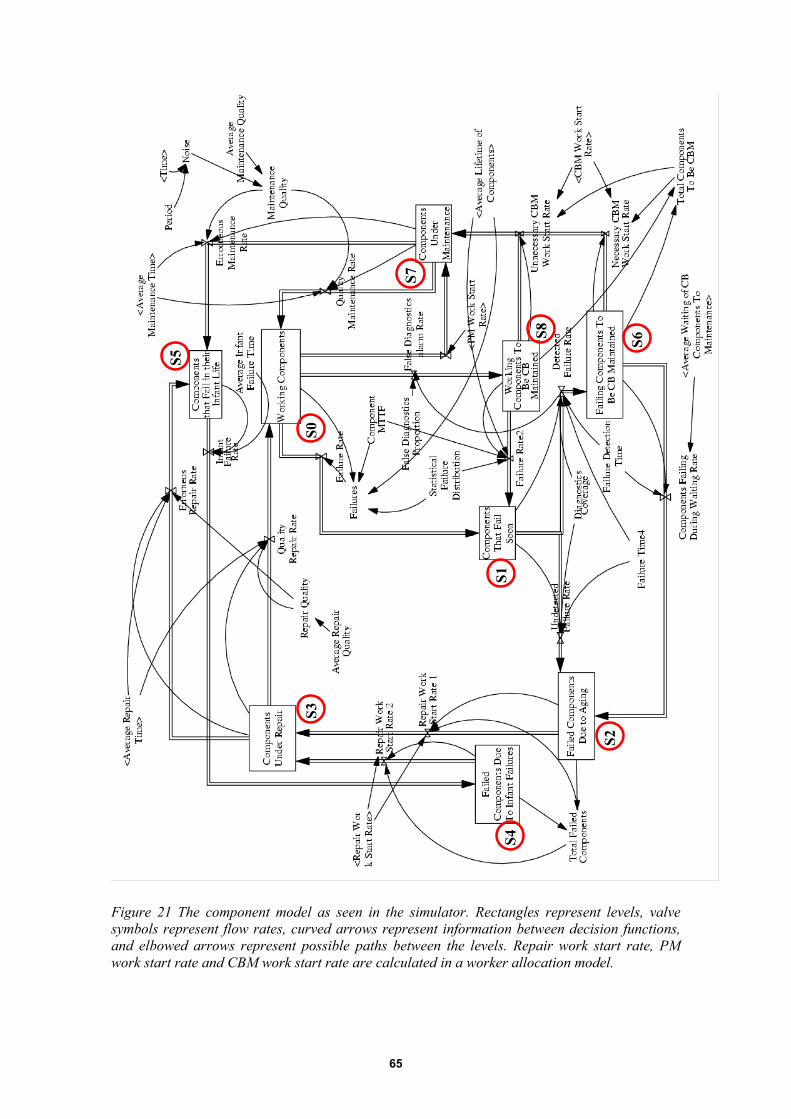
65

S0

S1

S2

S4

S3

S5

S6S8

S7

Figure 21 The component model as seen in the simulator. Rectangles represent levels, valvesymbols represent flow rates, curved arrows represent information between decision functions,and elbowed arrows represent possible paths between the levels. Repair work start rate, PMwork start rate and CBM work start rate are calculated in a worker allocation model.

66

State Description Characteristic state delayS0 Number of working components Defined by the average age of

components by equation (16) andthe renewal delay by equation(19)

S1 Number of components that fail soon 12 weeks failure delayS2 Number of failed components due to deterioration 1 week administration delayS3 Number of components under repair 3 weeks repair delayS4 Number of failed components due to infant failures 1 week administration delayS5 Number of components that fail in their infant life 5 weeks infant failure delayS6 Number of failing components to be maintained 1 week administration delay and

8 weeks detection delayS7 Number of components under maintenance 4 weeks maintenance delayS8 Number of working components to be maintained 1 week administration delayTable 6 The component states and the characteristic delays.

6.5.6 Worker allocation model

The components are being maintained by a 30-person group of workers who can be in threemodes: idling, repairing, and executing proactive maintenance. The respective states areW0…W2 that are defined by the number of workers in that mode. The state for the preventiveand condition-based maintenance actions is the same (W2) and requires one worker and fourweeks to complete. Repairing (W1) can be done in three weeks, but requires on average twopersons to complete. The administrative delay from start to end of a maintenance or repair task isone week. This time is spent in such activities as travelling, diagnosing the failures, andreporting the maintenance tasks. A simulator view of the worker allocation model is presented inFigure 22. The worker allocation states, characteristic delays and number of workers required tocomplete are presented in Table 7.

67

W0

W2

W1

Figure 22 The worker allocation model as seen in the simulator. PM work start rate is defined inthe control model.

State Description Characteristic state delay Workers requiredto complete

W0 Number of idle workers 1 week administration delayW1 Number of repair workers 3 weeks repair delay 2 workersW2 Number of proactive

maintenance workers4 weeks maintenance delay 1 worker

Table 7 The worker states, the characteristic delays and the required number of workers.

6.5.7 Deterioration failure process

It is assumed that there are one thousand components (C=1000) in the system. They are normallyin a working state (S0). However, due to deterioration they fail. The failure rate is a function ofthe average age of the components in operation. This is a rough simplification and does not takethe age distribution of the components into account, but nevertheless illustrates the effect of thepopulation age on the failure rate. The deterioration failure process is defined with a modifiedWeibull failure rate

1

),(−

⋅⋅=

β

ηηβλ xccx (16)

where x is the average age of the components and c is the number of working components.The used shape and scale parameters β=5 and η=566 make the curve steeply increasing todenote the effect of the high average age on the failures. Equation (16) and the shape and scaleparameter values are fictive. The failure process can be considered to be formed from c equally

68

old components that each have a failure pattern defined with a Weibull failure rate where β=5and η=566, which make the component MTTF equal to 520 weeks. A ten-year lifetime for anindustrial machine is quite common (Barringer, 2003).

The component state changes from working components (S0) to components that fail soon(S1) according to the deterioration process. The components that fail soon (S1) fail in average 12weeks unless detected by an automatic condition monitoring and diagnostics system that has anaverage 8-week fixed detection time before the failure. If the diagnostics does not detect thefailure, the component fails to the failed components due to deterioration state (S2) after eightweeks.

6.5.8 Repair process

The failed components are taken under the components under repair state (S3) if there are twoworkers available for that. The repair takes three weeks plus one additional week foradministrative delays. If the repair is successful, the component is restored back to the workingcomponents state (S0). Thinking this way, the components are restored without the use ofmaterials. Or, one may think that the component represents a function that can be in thepreviously described states, and the maintenance restores the function with the help of spareparts or new components that are immediately available from a local inventory.

6.5.9 Repeatability of repair actions

The repair may be unsuccessful with 10 % probability, in which case the component is taken intooperation but is in the components that fail in their infant life state (S5). In other words, therepeatability of the repair is 90 %. The average time the components operate in that state is fiveweeks after which the component fails to the failed components due to infant failures state (S4).The component is again repaired if there are two workers available. The selected repeatabilityrate may be too low if it were compared to the repair repeatability of real systems. However, thesystem behaviour is more easily visible with such parameter value selection.

6.5.10 Condition-based maintenance process

If the condition monitoring system detects the deterioration failure, the component is put in thefailing components to be maintained state (S6). If there is one worker available for condition-based maintenance, the component is moved to the components under maintenance state (S7). Inany case, the repair has a higher priority than condition-based maintenance and may cause ashortage of worker resources to condition-based maintenance of the components. The condition-based maintenance has, however, a higher priority than preventive maintenance. From thecomponents under maintenance state (S7) the component proceeds as in preventive maintenancedescribed in the next chapter. The condition monitoring may be tuned to be too sensitive andcause false alarms. This is modelled as a fixed ratio of the detected failures rate. In case of falsecondition monitoring alarms the component is moved from the working components state (S0) tothe working components to be maintained state (S8). The user cannot observe that state, so thecomponents in that state are processed with the same priority as the failing components to bemaintained (S6).

6.5.11 Preventive maintenance process

To prevent the deterioration failures the maintenance system may renew some proportion of theworking components to decrease the average age of the components. The components arechanged to the components under maintenance state (S7) if there is one worker available forpreventive maintenance. In any case, the repair and condition-based maintenance have a higher

69

priority and may cause a shortage of worker resources to preventive maintenance of thecomponents. The maintenance succeeds with 95 % probability, i.e. the repeatability of themaintenance actions is 95 %. After successful maintenance the component is returned to theworking components state (S0). If the maintenance is not successful, the component is moved tothe components that fail in their infant life state (S5) and consequently, it will participate in therepair process.

6.5.12 Preventive maintenance control model

Selecting a predefined preventive maintenance interval in the model is based on the assumptionthat there is some target control variable. This kind of an optimum setpoint value may comefrom such a model as presented in Chapter 6.4. In the model the controlled variable is defined by

)( fifdr nnnCY ++−= (17)

where C is the total number of components, nr is the number of components being repaired (S3),nfd is the number of components that have failed because of deterioration (S2) and nfi is thenumber of components failed because of infant failures (S4).

Considering the scope of this dissertation in process industries, the indirect costs of failuresare assumed relatively high compared to the costs of proactive maintenance. Therefore,proactive maintenance is preferred and the components under proactive maintenance are notincluded in (17). That is, the goal is not to control the operational availability but the reliability(MTTF).

The logic is to take the controlled reliability variable Y and compare it to a setpoint of adesired value. The difference, or error, between the actual value and the setpoint is controlled bychanging the preventive maintenance rate of the working components. The error equation isdefined as

SYE −= (18)

where S is the setpoint number of components, or the reliability target.Selection of the preventive maintenance interval proceeds as follows: if the error E is

positive, increase the maintenance interval to decrease reliability and therefore reduce Y. If theerror E is negative, decrease the maintenance interval. If the error E is zero, then the requiredlevel is achieved and no control action is needed. Control of the interval is continuous but thechanges are assumed very small. In practice the randomness in the failure process makes itdifficult to estimate the actual error value. Therefore, the measurements must be filtered toobtain the real error E.

The selected approach to model the control logic is a proportional-integral (PI) controlalgorithm (Åström and Hägglund, 2000) that is commonly used in industrial process control.The use of the PI-algorithm does not imply that in reality the preventive maintenance iscontrolled by using a PI-algorithm. Merely, the PI-algorithm simulates the real world decisionmaking and learning in which the system reliability is controlled with the help of some heuristicand mental processes. Usage of both proportional and integral control parameters filters high-frequency error signals out and ensures that the error will eventually be zero. A derivativeparameter is not used because its prediction capability by linear extrapolation is not veryeffective in slow processes.

Error E is used to control the renewal delay, e.g. the weeks to renew all the components, withthe PI equation (Åström and Hägglund, 2000) in parallel form:

70

MTTF)MTTF),0.4,G dt EGE+MTTF*7MAX(MIN(0.R(E) ip ⋅⋅+⋅= ∫ (19)

where the MTTF of a component is 520 weeks, Gp = 100 is the proportional error gain and Gi =2is the integral error gain. In other words, the error of one component causes one hundred weeks’change in the renewal delay, and one component-week integral error causes two weeks’ changein the renewal delay. These values were selected by testing the system so that there is some, butnot excessive oscillation in the preventive maintenance work start rate. Thus, the system isappropriately tuned.

The minimum and maximum rates for the renewal delay are 0.4⋅MTTF and 1⋅MTTF of thecomponent to prevent too long or short renewal delay. These limits are set by reasoning that thepreventive maintenance frequency cannot be too high or low. The initial renewal delay is 0.7⋅520weeks equalling to changing all the working components in 364 weeks. A simulator view of thecontrol algorithm is presented in Figure 23.

71

Figure 23 The simulator view of the PI-control algorithm. Setpoint S is set by adjusting thetarget percentage for operating and maintained components (Y).

6.5.13 Analysis of the system behaviour

The system is started from a situation where all the components are new and in the working state(S0). The controlled variable Y=997. In other words, only three components should be underrepair or waiting for repair. The simulation time is 3120 weeks equalling 60 years.

As shown by Figure 24 the system stabilisation takes almost thirty years. In the beginningthe components are new and no preventive maintenance is needed. However, the number ofdeterioration failures increases quickly when the average age of the components increases. Thisis compensated with a heavy preventive replacement policy, which causes the averagecomponent ages to drop. The behaviour of the preventive maintenance work start rate starts tooscillate. The highest amplitudes of the start rate for the preventive maintenance work are cutbecause of the limits defined in (19), and because of the shortage of workers for preventivemaintenance. Between week 980 (year 19) and week 1221 (year 23) there are not enoughworkers to do the required preventive maintenance. The system seems to be too slow.

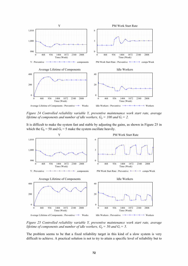
72

Y1,010

1,000

990

11

11

1 1 1 1 1 1 1

0 468 936 1404 1872 2340 2808Time (Week)

Y : Preventive components1 1 1 1 1 1

PM Work Start Rate6

3

0

1 1 1 1

1

1

11 1 1 1 1

0 468 936 1404 1872 2340 2808Time (Week)

PM Work Start Rate : Preventive comps/Week1 1 1

Average Lifetime of Components400

200

0 1

1

1 11 1 1 1 1 1 1 1

0 468 936 1404 1872 2340 2808Time (Week)

Average Lifetime of Components : Preventive Weeks1

Idle Workers40

20

0

11

1 1

1

11 1 1 1 1 1

0 468 936 1404 1872 2340 2808Time (Week)

Idle Workers : Preventive Workers1 1 1 1 1

Figure 24 Controlled reliability variable Y, preventive maintenance work start rate, averagelifetime of components and number of idle workers, Gp = 100 and Gi = 2.

It is difficult to make the system fast and stable by adjusting the gains, as shown in Figure 25 inwhich the Gp = 50 and Gi = 5 make the system oscillate heavily.

Y1,010

1,000

990

11

11

11

1 1 1 11

0 468 936 1404 1872 2340 2808Time (Week)

Y : Preventive components1 1 1 1 1 1

PM Work Start Rate6

3

0

1 1 1 1

11

1

11

1

1

1

0 468 936 1404 1872 2340 2808Time (Week)

PM Work Start Rate : Preventive comps/Week1 1 1

Average Lifetime of Components400

200

0 1

1

1 11

1

1 11

1

1

1

0 468 936 1404 1872 2340 2808Time (Week)

Average Lifetime of Components : Preventive Weeks1

Idle Workers40

20

0

11

1 1

1 1

1

1 11

1

1

0 468 936 1404 1872 2340 2808Time (Week)

Idle Workers : Preventive Workers1 1 1 1 1

Figure 25 Controlled reliability variable Y, preventive maintenance work start rate, averagelifetime of components and number of idle workers, Gp = 50 and Gi = 5.

The problem seems to be that a fixed reliability target in this kind of a slow system is verydifficult to achieve. A practical solution is not to try to attain a specific level of reliability but to

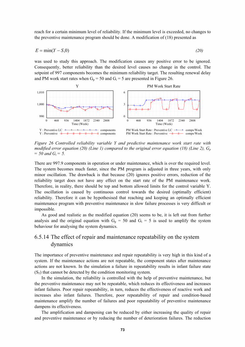
73

reach for a certain minimum level of reliability. If the minimum level is exceeded, no changes tothe preventive maintenance program should be done. A modification of (18) presented as

)0,min( SYE −= (20)

was used to study this approach. The modification causes any positive error to be ignored.Consequently, better reliability than the desired level causes no change in the control. Thesetpoint of 997 components becomes the minimum reliability target. The resulting renewal delayand PM work start rates when Gp = 50 and Gi = 5 are presented in Figure 26.

Y1,010

1,000

990

22

2 22 2

22 2 2 2

1 11 1 1 1 1 1 1 1 1

0 468 936 1404 1872 2340 2808Time (Week)

Y : Preventive LC components1 1 1 1 1 1Y : Preventive components2 2 2 2 2 2 2

PM Work Start Rate6

3

0

2 2 2 2

22

2

2

2

22

21 1 1

1 1 1 1 1 1 1 1 1

0 468 936 1404 1872 2340 2808Time (Week)

PM Work Start Rate : Preventive LC comps/Week1 1PM Work Start Rate : Preventive comps/Week2 2

Figure 26 Controlled reliability variable Y and predictive maintenance work start rate withmodified error equation (20) (Line 1) compared to the original error equation (18) (Line 2), Gp= 50 and Gi = 5.

There are 997.9 components in operation or under maintenance, which is over the required level.The system becomes much faster, since the PM program is adjusted in three years, with onlyminor oscillation. The drawback is that because (20) ignores positive errors, reduction of thereliability target does not have any effect on the start rate of the PM maintenance work.Therefore, in reality, there should be top and bottom allowed limits for the control variable Y.The oscillation is caused by continuous control towards the desired (optimally efficient)reliability. Therefore it can be hypothesised that reaching and keeping an optimally efficientmaintenance program with preventive maintenance in slow failure processes is very difficult orimpossible.

As good and realistic as the modified equation (20) seems to be, it is left out from furtheranalysis and the original equation with Gp = 50 and Gi = 5 is used to amplify the systembehaviour for analysing the system dynamics.

6.5.14 The effect of repair and maintenance repeatability on the systemdynamics

The importance of preventive maintenance and repair repeatability is very high in this kind of asystem. If the maintenance actions are not repeatable, the component states after maintenanceactions are not known. In the simulation a failure in repeatability results in infant failure state(S5) that cannot be detected by the condition monitoring system.

In the simulation, the reliability is controlled with the help of preventive maintenance, butthe preventive maintenance may not be repeatable, which reduces its effectiveness and increasesinfant failures. Poor repair repeatability, in turn, reduces the effectiveness of reactive work andincreases also infant failures. Therefore, poor repeatability of repair and condition-basedmaintenance amplify the number of failures and poor repeatability of preventive maintenancedampens its effectiveness.

The amplification and dampening can be reduced by either increasing the quality of repairand preventive maintenance or by reducing the number of deterioration failures. The reduction

74

of deterioration failures takes place through preventive maintenance, which increases the numberof infant failures. If the quality of repair and preventive maintenance cannot be increased, acontrol action out of the system scope, such as better component design, is required.

If the repair and maintenance quality is 100 %, i.e. fully repeatable, the system behaves asshown in Figure 27. Because the preventive maintenance does not cause infant failures, thedeterioration failures are increased with a slower rate. The preventive maintenance is moreeffective and therefore the number of failures decreases more rapidly. Consequently, theamplification of the system is lower and the system is easier to control. In fact, the systemcontrol does not take into account that there are two failure types: infant failures caused bymaintenance errors and deterioration failures.

Y1,010

1,000

990

22

2 22 2

22 2 2 2

1 11 1 1 1

1 1 1 1 1

0 468 936 1404 1872 2340 2808Time (Week)

Y : Preventive HQ components1 1 1 1 1Y : Preventive components2 2 2 2 2 2 2

Repair Workers8

4

0 2

2

2

2

2

2

2 2

2

2

2

2

11

1

1 1 1

11

1 11 1

0 468 936 1404 1872 2340 2808Time (Week)

Repair Workers : Preventive HQ Workers1 1 1 1Repair Workers : Preventive Workers2 2 2 2

Average Lifetime of Components400

200

02

2

2 2

22

22

2 2 2

1

1

1 1 1 11

1 1 1 1 1

0 468 936 1404 1872 2340 2808Time (Week)

Average Lifetime of Components : Preventive HQ Weeks1Average Lifetime of Components : Preventive Weeks2

Idle Workers40

20

0

2 22 2

2 2

2

2

2

22

2

1 11 1 1 1

1

1 1 1 1 1

0 468 936 1404 1872 2340 2808Time (Week)

Idle Workers : Preventive HQ Workers1 1 1 1Idle Workers : Preventive Workers2 2 2 2

Figure 27 Controlled reliability variable Y, number of repair workers, average lifetime ofcomponents, and number of idle workers with 100 % maintenance and repair quality (Line 1)compared to 95 % maintenance and 90 % repair quality (Line 2), error equation (18), Gp = 50and Gi = 5.

6.5.15 The effect of condition monitoring on the system dynamics

The installation of a condition monitoring system shifts a certain proportion of the reactivemaintenance actions to proactive maintenance. Therefore, increasing the diagnostics coveragereduces failures, which further dampens the amplification caused by poor repeatability of repair.However, possible false diagnostics alarms cause unnecessary condition-based maintenanceactions. If successful, these actions decrease the average age of the components and thereforedecrease the number of deterioration failures. If unsuccessful, the number of infant failures isincreased. If the increase of the infant failures is lower than the reduction of the deteriorationfailures, the false alarms increase reliability. In case of a constant failure rate, no preventivemaintenance can increase reliability. In that case, false diagnostics increases the number offailures if the maintenance repeatability is not 100 %. If the failure rate is decreasing falsediagnostics increases the number of failures in any case. In other words, perfect conditionmonitoring dampens the reliability oscillations caused by imperfect repeatability of the repairwork.

75

The effect of 15 % diagnostics coverage without false alarms is shown in Figure 28. Thesystem oscillation is dampened. Some of the repair workers are moved to condition-basedmaintenance and less preventive maintenance is required. Increasing the number of false alarmsup to 20 times the detected failures did not have any other effect than increasing the systemreliability and reducing the average age of the components. A test with a constant failure rateshowed that the reliability was reduced if there were false alarms.

Y1,010

1,000

990

22

2 22 2

22 2 2 2

1 11 1 1 1 1 1 1 1 1

0 468 936 1404 1872 2340 2808Time (Week)

Y : Preventive DC=15% components1 1 1 1Y : Preventive components2 2 2 2 2 2 2

Repair Workers8

4

0 2

2

2

2

2

2

2 2

2

2

2

2

1

1

1

1 1 1 1 1

1

11

1

0 468 936 1404 1872 2340 2808Time (Week)

Repair Workers : Preventive DC=15% Workers1 1Repair Workers : Preventive Workers2 2 2 2

Average Lifetime of Components400

200

02

2

2 22

2

22 2

22

2

1

1

1 1 1 1 1 11

11

1

0 468 936 1404 1872 2340 2808Time (Week)

Average Lifetime of Components : Preventive DC=15% WeeksAverage Lifetime of Components : Preventive Weeks2

Maintenance Workers20

10

0

2 2 2 2

22

2

2

2

2 2

21 1 1 1 1 1 1 1

1 1 1 1

0 468 936 1404 1872 2340 2808Time (Week)

Maintenance Workers : Preventive DC=15% Workers1Maintenance Workers : Preventive Workers2 2 2

Figure 28 Controlled reliability variable Y, number of repair workers, average lifetime ofcomponents and number of maintenance workers when diagnostics coverage is 15 % (Line 1)compared to 0 % diagnostics coverage (Line 2), error equation (18), Gp = 50 and Gi = 5.

6.5.16 The effect of insufficient work resources on the system dynamics

Preventive maintenance controls the reliability. Because preventive maintenance has the lowestpriority of the maintenance work, a sudden increase in deterioration or infant failures may leadto a shortage of resources in preventive maintenance. In this case, the system controllability isreduced until the failures have been repaired. Thinking in a systemic sense, this means that thecoupling of preventive maintenance via the deterioration failure process to reactive maintenanceis reversed so that reactive maintenance is coupled to preventive maintenance via a shortage ofwork resources.

In Figure 29 there are 35 maintenance workers instead of 30 maintenance workers. Thetarget reliability is achieved sooner because there are enough maintenance workers, which makesit possible to do more preventive maintenance work. The reduction rate is the same because thedeterioration failure process defines the dynamics of decreasing reliability.

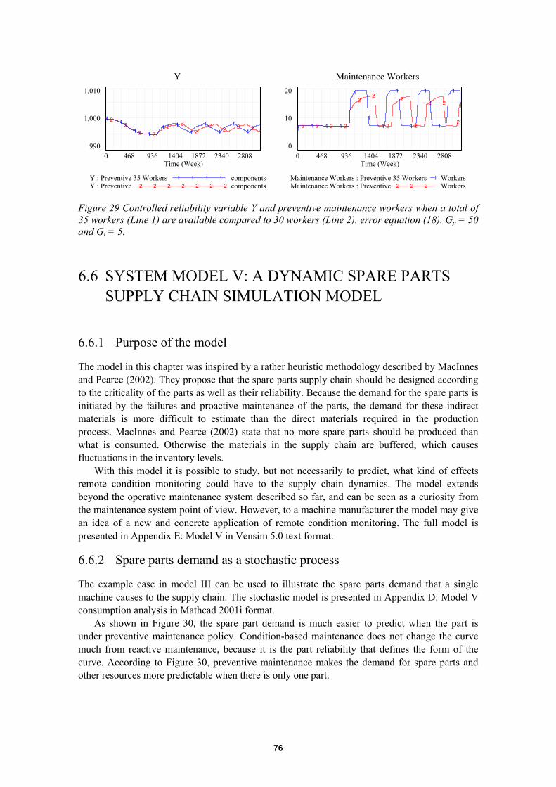
76

Y1,010

1,000

990

22

2 22 2

22 2 2 2

1 11 1

1 11

11

11

0 468 936 1404 1872 2340 2808Time (Week)

Y : Preventive 35 Workers components1 1 1 1Y : Preventive components2 2 2 2 2 2 2

Maintenance Workers20

10

0

2 2 2 2

22

2

2

2

2 2

21 1 1 1

1

11

1

1

1

1

1

0 468 936 1404 1872 2340 2808Time (Week)

Maintenance Workers : Preventive 35 Workers Workers1Maintenance Workers : Preventive Workers2 2 2

Figure 29 Controlled reliability variable Y and preventive maintenance workers when a total of35 workers (Line 1) are available compared to 30 workers (Line 2), error equation (18), Gp = 50and Gi = 5.

6.6 SYSTEM MODEL V: A DYNAMIC SPARE PARTSSUPPLY CHAIN SIMULATION MODEL

6.6.1 Purpose of the model

The model in this chapter was inspired by a rather heuristic methodology described by MacInnesand Pearce (2002). They propose that the spare parts supply chain should be designed accordingto the criticality of the parts as well as their reliability. Because the demand for the spare parts isinitiated by the failures and proactive maintenance of the parts, the demand for these indirectmaterials is more difficult to estimate than the direct materials required in the productionprocess. MacInnes and Pearce (2002) state that no more spare parts should be produced thanwhat is consumed. Otherwise the materials in the supply chain are buffered, which causesfluctuations in the inventory levels.

With this model it is possible to study, but not necessarily to predict, what kind of effectsremote condition monitoring could have to the supply chain dynamics. The model extendsbeyond the operative maintenance system described so far, and can be seen as a curiosity fromthe maintenance system point of view. However, to a machine manufacturer the model may givean idea of a new and concrete application of remote condition monitoring. The full model ispresented in Appendix E: Model V in Vensim 5.0 text format.

6.6.2 Spare parts demand as a stochastic process

The example case in model III can be used to illustrate the spare parts demand that a singlemachine causes to the supply chain. The stochastic model is presented in Appendix D: Model Vconsumption analysis in Mathcad 2001i format.

As shown in Figure 30, the spare part demand is much easier to predict when the part isunder preventive maintenance policy. Condition-based maintenance does not change the curvemuch from reactive maintenance, because it is the part reliability that defines the form of thecurve. According to Figure 30, preventive maintenance makes the demand for spare parts andother resources more predictable when there is only one part.

77

0 2000 4000 60000

0.2

0.4

0.6

0.8

11

0

pi

2MTTF comp0 ti

0 2000 4000 60000

0.2

0.4

0.6

0.8

11

0

pi

2MTTF comp0 ti

Figure 30 Probability of spare part demand of reactive (left) and preventive (right) maintenancepolicies.

The more there are part usage locations that the supply chain serves, the more evenly andrandomly the failure and maintenance intervals will be distributed. Therefore, it can be assumedthat when there are several part usage locations, the demand interarrival times for a spare part areexponentially distributed as presented in Figure 31. That is, with many parts operating, failingand being maintained independently the interarrival times converge to an exponentialdistribution with a mean value that equals the mean life time of the parts divided by the numberof the parts regardless of the applied maintenance policies.

0 50 1000

0.2

0.4

0.6

0.8

11

0

pexp ti1

µ group,

pi

µ group 3 σ group⋅+0 ti

Figure 31 Analytically calculated exponential demand interval (dotted line) and simulateddemand interval (solid line) in calendar days of 100 parts for 1000 years under conditionmonitoring and preventive maintenance. The average failure interval µgroup=30.853 is calculatedfrom simulation. µgroup ≈ 1/100 ⋅ mean failure or maintenance interval 3070.991 for one part.The visible error comes from inaccuracy of the numerical simulation.

The inventories use buffering to match the uncertainty in the demand and supply. Therefore, theinterarrival times between the orders that an upper stream inventory sees from each serveddownstream inventory can be modelled with a Gamma distribution. The distribution parametersare defined by the demand that the downstream inventory sees and the order quantity (OQ) thatthe downstream inventory uses. With OQ=1, the demand interval follows an exponentialdistribution, with OQ>=1 the demand interval follows a Gamma distribution. According to thecentral limit theorem with OQ >> 1, the demand interval can be approximated with a normaldistribution, where mean = OQ ⋅ mean of the exponential distribution and standard deviation issqrt(OQ) ⋅ mean of the exponential distribution. All these are special cases of a Gammadistribution.

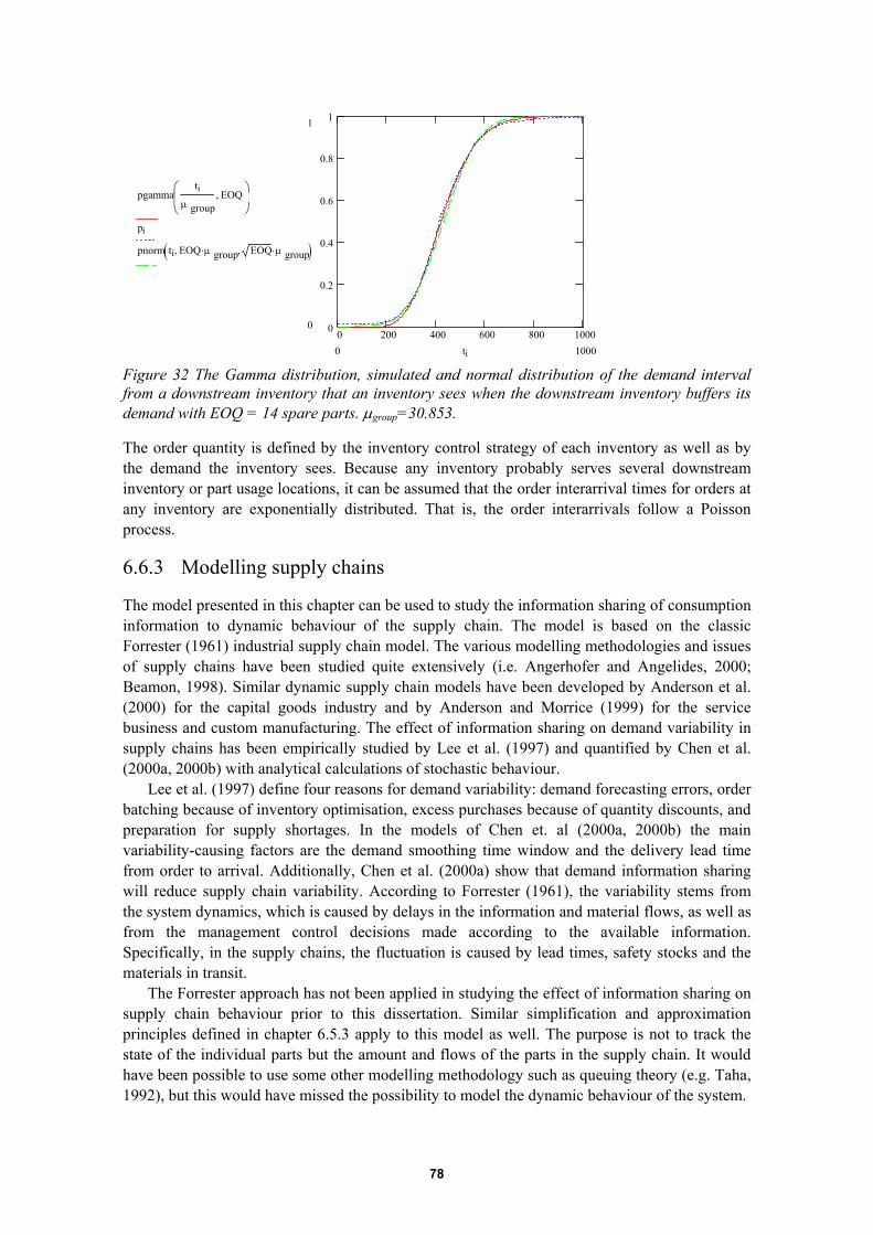
78

0 200 400 600 800 10000

0.2

0.4

0.6

0.8

11

0

pgammati

µ groupEOQ,

pi

pnorm ti EOQ µ group⋅, EOQ µ group⋅,( )

10000 ti

Figure 32 The Gamma distribution, simulated and normal distribution of the demand intervalfrom a downstream inventory that an inventory sees when the downstream inventory buffers itsdemand with EOQ = 14 spare parts. µgroup=30.853.

The order quantity is defined by the inventory control strategy of each inventory as well as bythe demand the inventory sees. Because any inventory probably serves several downstreaminventory or part usage locations, it can be assumed that the order interarrival times for orders atany inventory are exponentially distributed. That is, the order interarrivals follow a Poissonprocess.

6.6.3 Modelling supply chains

The model presented in this chapter can be used to study the information sharing of consumptioninformation to dynamic behaviour of the supply chain. The model is based on the classicForrester (1961) industrial supply chain model. The various modelling methodologies and issuesof supply chains have been studied quite extensively (i.e. Angerhofer and Angelides, 2000;Beamon, 1998). Similar dynamic supply chain models have been developed by Anderson et al.(2000) for the capital goods industry and by Anderson and Morrice (1999) for the servicebusiness and custom manufacturing. The effect of information sharing on demand variability insupply chains has been empirically studied by Lee et al. (1997) and quantified by Chen et al.(2000a, 2000b) with analytical calculations of stochastic behaviour.

Lee et al. (1997) define four reasons for demand variability: demand forecasting errors, orderbatching because of inventory optimisation, excess purchases because of quantity discounts, andpreparation for supply shortages. In the models of Chen et. al (2000a, 2000b) the mainvariability-causing factors are the demand smoothing time window and the delivery lead timefrom order to arrival. Additionally, Chen et al. (2000a) show that demand information sharingwill reduce supply chain variability. According to Forrester (1961), the variability stems fromthe system dynamics, which is caused by delays in the information and material flows, as well asfrom the management control decisions made according to the available information.Specifically, in the supply chains, the fluctuation is caused by lead times, safety stocks and thematerials in transit.

The Forrester approach has not been applied in studying the effect of information sharing onsupply chain behaviour prior to this dissertation. Similar simplification and approximationprinciples defined in chapter 6.5.3 apply to this model as well. The purpose is not to track thestate of the individual parts but the amount and flows of the parts in the supply chain. It wouldhave been possible to use some other modelling methodology such as queuing theory (e.g. Taha,1992), but this would have missed the possibility to model the dynamic behaviour of the system.

79

6.6.4 Model overview

The presented model is a simplified version of the Forrester (1961) model. The simplificationsmean that the orders from the downstream inventories to the upstream inventories are transferredand processed immediately. The delay times are also different from Forrester's model. Therewere two reasons for the simplification: firstly, electronic orders have been introduced and takeninto use in industrial supply chains, and secondly, the problem is not to model the effect of theorder processing but the effect of the information provided by remote condition monitoring forthe system. The model parameters are fictive, but not unrealistic, serving the purpose of themodel.

The model was developed and simulated with Vensim PLE v5.01 by Ventana Systems Inc.A simulator view of model is presented in Figure 33 and a simplified version of the systemmodel is presented in Figure 34. The system models a supply chain consisting of three levels ofinventories: manufacturer inventory (Level 1), regional distributor inventories (Level 2) andplant inventories (Level 3).

80

Figure 33 The supply chain model as seen in the simulator.

81

MANUF.INVENTORY

INSTALLEDBASE

CONSUMPTION

Lev el1 Lev el 2 Lev el 3

ORDERSORDERSORDERS

MATERIALS MATERIALSMATERIALS MATERIALS

PRODUCTION

CONSUMPTION INFORMATIONFROM MACHINES TO MANUFACTURER VIA

REMOTE CONDITION MONITORING

CONSUMPTION INFORMATIONSHARED BY MANUFACTURER TO

SUPPLY CHAIN

REGIONALINVENTORIES PLANT

INVENTORIES

Figure 34 A simplified view of the supply chain model.

It is assumed in the model that there is an installed base of 90,000 parts. Each part has a failuretype that is prevented or reacted to by replacing the part with a new one. The mean lifetime ofthe parts is 3,000 calendar days. Therefore, the parts are replaced at the average rate of 30 partsper day. The plant inventories store some parts as an insurance stock. The assumption is that thespare parts are not stocked by the maintenance on the factory floor after taken from theinventory. If the insurance stock falls below a predefined limit, an order is placed with a regionalparts provider. If the stock of a regional inventory falls below a predefined limit, an order isplaced with the manufacturer. An economic order quantity (EOQ) model (Beyer and Sethi,1998) or similar is used to determine the inventory levels and order quantities. The manufacturerinventory uses a similar order quantity strategy to order parts from its production department thathas a maximum production capacity of 37.5 parts / day, which is 25 % more than the averagedemand.

Because an inventory must serve very reliably the next level inventories, the inventory levelmust be kept high enough to compensate the randomness in supply and consumption to maintainthe required service level. Therefore, there are always more parts in the supply chain than theaverage consumption would require. There are also some parts under transportation between theinventories, which can be seen as a supply pipeline that must be filled or emptied if the averageconsumption rate changes. Each inventory notes that there may be random fluctuation in theorders. Therefore they smooth the number of orders with 3rd order exponential smoothing, thatweights more the recent consumption, to estimate the average demand. The difference betweenthe desired inventory level and the actual inventory level is corrected after some time, defined bythe average time to accumulate a demand that equals the order quantity (OQ) amount of parts.This correction time can also be seen as the delay that corrects the difference between thedesired and actual inventory. E.g. a 10-day correction delay corrects the difference at the rate of10 %/day. The orders are processed immediately and sent to the next level inventory. Thetransportation takes some time, which is modelled with 3rd order delay. The inventory target ismodelled with

det TDKI ⋅⋅= (21)

where K is the safety factor for random fluctuation, De is the estimated demand / day, and Td isthe transportation delay from the upper stream inventory or the delay of the production process.

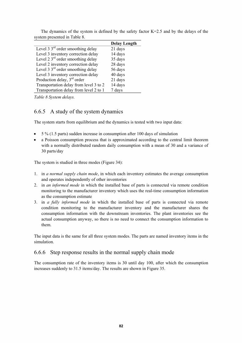
82

The dynamics of the system is defined by the safety factor K=2.5 and by the delays of thesystem presented in Table 8.

Delay LengthLevel 3 3rd order smoothing delay 21 daysLevel 3 inventory correction delay 14 daysLevel 2 3rd order smoothing delay 35 daysLevel 2 inventory correction delay 28 daysLevel 3 3rd order smoothing delay 56 daysLevel 3 inventory correction delay 40 daysProduction delay, 3rd order 21 daysTransportation delay from level 3 to 2 14 daysTransportation delay from level 2 to 1 7 days

Table 8 System delays.

6.6.5 A study of the system dynamics

The system starts from equilibrium and the dynamics is tested with two input data:

• 5 % (1.5 parts) sudden increase in consumption after 100 days of simulation• a Poisson consumption process that is approximated according to the central limit theorem

with a normally distributed random daily consumption with a mean of 30 and a variance of30 parts/day

The system is studied in three modes (Figure 34):

1. in a normal supply chain mode, in which each inventory estimates the average consumptionand operates independently of other inventories

2. in an informed mode in which the installed base of parts is connected via remote conditionmonitoring to the manufacturer inventory which uses the real-time consumption informationas the consumption estimate

3. in a fully informed mode in which the installed base of parts is connected via remotecondition monitoring to the manufacturer inventory and the manufacturer shares theconsumption information with the downstream inventories. The plant inventories see theactual consumption anyway, so there is no need to connect the consumption information tothem.

The input data is the same for all three system modes. The parts are named inventory items in thesimulation.

6.6.6 Step response results in the normal supply chain mode

The consumption rate of the inventory items is 30 until day 100, after which the consumptionincreases suddenly to 31.5 items/day. The results are shown in Figure 35.

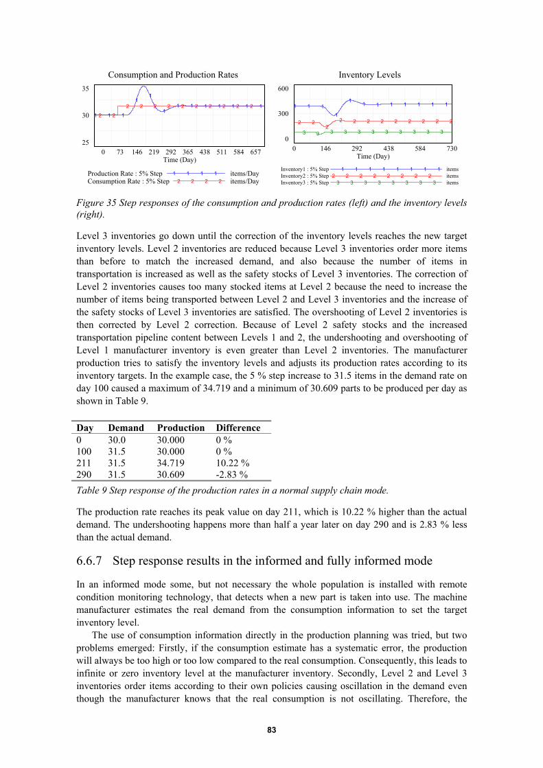
83

Consumption and Production Rates35

30

25

2 2

2 2 2 2 2 2 2 2 2 2

1 1 1

11

11 1 1 1 1 1 1

0 73 146 219 292 365 438 511 584 657Time (Day)

Production Rate : 5% Step items/Day1 1 1 1Consumption Rate : 5% Step items/Day2 2 2 2

Inventory Levels600

300

03 3 3 3 3 3 3 3 3 3 3

2 22

2 2 2 2 2 2 2 2 2

1 1 11

1 1 1 1 1 1 1 1

0 146 292 438 584 730Time (Day)

Inventory1 : 5% Step items1 1 1 1 1 1 1 1Inventory2 : 5% Step items2 2 2 2 2 2 2 2Inventory3 : 5% Step items3 3 3 3 3 3 3 3

Figure 35 Step responses of the consumption and production rates (left) and the inventory levels(right).

Level 3 inventories go down until the correction of the inventory levels reaches the new targetinventory levels. Level 2 inventories are reduced because Level 3 inventories order more itemsthan before to match the increased demand, and also because the number of items intransportation is increased as well as the safety stocks of Level 3 inventories. The correction ofLevel 2 inventories causes too many stocked items at Level 2 because the need to increase thenumber of items being transported between Level 2 and Level 3 inventories and the increase ofthe safety stocks of Level 3 inventories are satisfied. The overshooting of Level 2 inventories isthen corrected by Level 2 correction. Because of Level 2 safety stocks and the increasedtransportation pipeline content between Levels 1 and 2, the undershooting and overshooting ofLevel 1 manufacturer inventory is even greater than Level 2 inventories. The manufacturerproduction tries to satisfy the inventory levels and adjusts its production rates according to itsinventory targets. In the example case, the 5 % step increase to 31.5 items in the demand rate onday 100 caused a maximum of 34.719 and a minimum of 30.609 parts to be produced per day asshown in Table 9.

Day Demand Production Difference0 30.0 30.000 0 %100 31.5 30.000 0 %211 31.5 34.719 10.22 %290 31.5 30.609 -2.83 %Table 9 Step response of the production rates in a normal supply chain mode.

The production rate reaches its peak value on day 211, which is 10.22 % higher than the actualdemand. The undershooting happens more than half a year later on day 290 and is 2.83 % lessthan the actual demand.

6.6.7 Step response results in the informed and fully informed mode

In an informed mode some, but not necessary the whole population is installed with remotecondition monitoring technology, that detects when a new part is taken into use. The machinemanufacturer estimates the real demand from the consumption information to set the targetinventory level.

The use of consumption information directly in the production planning was tried, but twoproblems emerged: Firstly, if the consumption estimate has a systematic error, the productionwill always be too high or too low compared to the real consumption. Consequently, this leads toinfinite or zero inventory level at the manufacturer inventory. Secondly, Level 2 and Level 3inventories order items according to their own policies causing oscillation in the demand eventhough the manufacturer knows that the real consumption is not oscillating. Therefore, the

84

manufacturer must supply the ordered items and produce a different number of items than theactual consumption would require.

In an informed mode the demand from Level 2 inventories to Level 1 manufacturerinventory remains the same, but the manufacturer production is controlled through the inventorytarget equation

dat TCKI ⋅⋅= (22)

where Ca is the actual daily consumption received via remote condition monitoring, and Td is thedelay of the production process for the manufacturer inventory. Safety factor K compensates therandom fluctuation and systematic errors in the actual consumption measurement.

Table 10 summarises the effect of connecting the consumption information to Level 3inventory target calculation. The peak production rate of 33.594 items /day on day 210 is 6.65 %higher than the actual consumption. The undershooting is only -0.67 %.

Day Demand Production Difference0 30.0 30.000 0 %100 31.5 30.000 0 %210 31.5 33.594 6.65 %298 31.5 31.290 -0.67 %Table 10 Step response of the production rates in an informed mode.

In Table 11, the manufacturer shares the consumption information with Level 2 inventories inorder to reduce the oscillation in the demand from Level 2. Level 2 inventories use the availableconsumption information in their inventory target calculations similarly to the manufacturerinventory. Because Level 3 inventories see the consumption directly, the whole supply chain isfully informed about the real consumption. The overshooting of the production is further reducedfrom 6.65 % to 5.82 % on day 210 and the undershooting reduces to -0.33 %.

Day Demand Production Difference0 30.0 30.000 0 %100 31.5 30.000 0 %210 31.5 33.332 5.82 %310 31.5 31.395 -0.33 %Table 11 Step response of the production rates in a fully informed mode.

As Figure 36 shows, the main reduction in the oscillation is achieved by connecting theconsumption to the manufacturer inventory. Information sharing with Level 2 inventoriesreduces the oscillation slightly further.

85

Production Rate40

35

30

25

20

3 3 3 3 33

33

33 3 3 3 3 3 3 3 3 3 3 3 3 3 3 3 3

2 2 2 2 22

2

22

22 2 2 2 2 2 2 2 2 2 2 2 2 2 2 2 2

1 1 1 1 1 1

1

11

1

1 11 1 1 1 1 1 1 1 1 1 1 1 1 1 1

0 73 146 219 292 365 438 511 584 657 730Time (Day)

Production Rate : 5% Step items/Day1 1 1 1 1 1 1 1 1 1 1 1 1 1 1 1 1 1 1Production Rate : 5% Step Monit items/Day2 2 2 2 2 2 2 2 2 2 2 2 2 2 2 2 2 2Production Rate : 5% Step Monit Shared items/Day3 3 3 3 3 3 3 3 3 3 3 3 3 3 3 3

Figure 36 Step response of the production rate in the normal (Line 1), informed (Line 2) andfully informed (Line 3) modes.

6.6.8 Random data responses in the informed and fully informed modes

A step test does not reveal all the system dynamics, however. To study the real effect ofcondition monitoring and information sharing a random consumption with a mean value andvariance of 30 items/day is applied to the three system modes. The consumption data is whitenoise as shown in Figure 37.

Consumption Rate60

30

0

1 11

1 11

1

1

11

11

0 146 292 438 584 730Time (Day)

Consumption Rate : Random items/Day1 1 1 1

Figure 37 Random consumption with 30 items / day as the mean value and variance.

The production rates and inventory levels of each system mode are shown inFigure 38 and Figure 39. As indicated by the step tests, the fully informed mode is the moststable in respect to the production rates and the manufacturer inventory levels.

86

Production Rate40

35

30

25

20

3 3

3 3

3

3

3

3

3 33

33

3

3

33

3

3

33

3

33

3

3

2 22

2

2

22

2

2 2 22 2

2

2

2

2

2

2

22

2

2

22

2

2

1 1 1

11

1

1

1

11

1 1

1

1

11

1 1

1

1

11

1

11

1

1

0 73 146 219 292 365 438 511 584 657 730Time (Day)

Production Rate : Random items/Day1 1 1 1 1 1 1 1 1 1 1 1 1 1 1 1 1 1 1Production Rate : Random Monit items/Day2 2 2 2 2 2 2 2 2 2 2 2 2 2 2 2 2 2Production Rate : Random Monit Shared items/Day3 3 3 3 3 3 3 3 3 3 3 3 3 3 3 3

Figure 38 Production rates in the normal (Line 1), informed (Line 2) and fully informed (Line 3)mode with the random consumption data.

Inventory1600

450

300

150

0

33

3

3

3

3

3

33 3 3 3

33

3

3

3

3

3 3

3

3 3

3

33

2 2

2 2

22

2

2 2

2 22

2

22

2

2

2

22 2

2

22

2

2

1 11

1

1

1

1

11

11

1

1

1 1

1 1

1

11

1

1

1

1

1

1

1

0 73 146 219 292 365 438 511 584 657 730Time (Day)

Inventory1 : Random items1 1 1 1 1 1 1 1 1 1 1 1 1 1 1 1 1 1 1 1 1Inventory1 : Random Monit items2 2 2 2 2 2 2 2 2 2 2 2 2 2 2 2 2 2 2 2Inventory1 : Random Monit Shared items3 3 3 3 3 3 3 3 3 3 3 3 3 3 3 3 3 3

Figure 39 Manufacturer inventory levels in the normal (Line 1), informed (Line 2) and fullyinformed (Line 3) modes with the random consumption data.

The numerical comparisons are presented in Table 12 and Table 13. Because the sample size islimited, the average production rates and inventory levels differ from the long-time averagevalues 30.0 and 375.0.

87

Average production rate (items/day) Standard deviationNormal mode 30.328 3.402Informed mode 30.332 2.316Fully informed mode 30.329 2.113Table 12 Average production rates and standard deviations in the normal, informed and fullyinformed modes with the random consumption data for 730 days.

Average inventory level (items) Standard DeviationNormal mode 370.490 101.130Informed mode 370.940 75.989Fully informed mode 371.557 65.182Table 13 Average manufacturer inventory levels and standard deviations in the normal,informed and fully informed modes with the random consumption data for 730 days.

The average level of manufacturer inventory in all three modes seems to be too high. Theoptimal average inventory level calculated with 99.5 % availability (stdev⋅2.58), and averagecapital value calculated with a fictive item value of Eur 25,000 are presented in Table 14. Theresults that cannot be seen from the step test are very interesting: the optimal average inventorylevel drops to 75.1 % and further to 64.5 % of the optimal values of the normal mode releasing amaximum capital of Eur 2,318,639 from the inventory. With 15 % own capital cost this wouldyield yearly additional savings of Eur 347,795.

Optimal averageinventory level (items)

Average capital value(Eur)

Proportion ofnormal mode

Normal mode 260.916 6,522,909 0 %Informed mode 196.051 4,901,267 75.1 %Fully informed mode 168.171 4,204,269 64.5 %Table 14 Optimal manufacturer inventory levels and capital value in the normal, informed andfully informed modes

In practice, the reduction of the inventory levels takes place through the reduction of safetyfactors K (21) (22) that partly define the variability of the system. Therefore, the reduction of Kreduces the deviations even more than in the presented Table 12 and Table 13. However, Table14 can be considered as a good approximation of a minimum inventory level reduction.

In summary, the simulation results allow to state that using the real-time materialconsumption information received via remote condition monitoring as a demand estimatereduces the upstream supply chain variability of the maintenance materials.

6.6.9 Further considerations

In the normal mode, reduction of smoothing delays of all the inventories to 21 days from theoriginal 56, 35 and 21 days reduces the manufacturer inventory standard deviation to 75.090. Ifcomparing this value to Table 14, it can be seen that the value is less than in the normal andinformed mode with the original smoothing delays. This indicates that too long a delay indemand averaging may increase the supply chain variability, which is an observation made byChen et. al (2000b). In the fully informed mode, the 21 days data smoothing results in a standarddeviation of 40.507 which represents a 53.9 % proportion of the normal mode. The proportionalreduction is higher than in Table 14 with the original smoothing delays. The reason for this isthat the use of real-time consumption information at 1st (manufacturer) and 2nd level inventoriesmakes it feasible to use shorter smoothing delays, which decreases the supply chain variability.

88

In other words, the use of real-time consumption also enables the reduction of the demandaveraging delays, which in turn reduces the variability even more.

If the inventory correction delays are halved, the respective standard deviations for themanufacturer inventory in the normal mode and the fully informed mode are increased to206.450 and 104.902. That is, if controlling a slow system too quickly, the system disturbanceswill be amplified, which supports the observations of Forrester (1961).

6.6.10 Summary and comparison to the results of other similar studies

Remote condition monitoring can be used for reducing the variability of the spare parts supplychain. The possible reduction in the inventory levels can be significant, especially if the actualconsumption information is shared with all the inventory levels. Furthermore, the use of real-time consumption enables the reduction of the demand averaging delays, which also reduces thesupply chain variability. The model results support the findings of Lee et al. (1997), Chen et al.(2000a, 2000b) and Forrester (1961) specified in chapters 6.6.3 and 6.6.9. The main contributionof the model is to study the practical idea that remote information acquisition of the spare partscan be used also for a direct benefit to the machine manufacturer without any maintenance-related service business between the manufacturer and the machine user. Furthermore, supplychain optimisation does not require changes in the business strategy of the machinemanufacturer.

89

7 DISCUSSION AND CONCLUSIONS

The viewpoint of this research was that of maintenance systems and system control. The effectof condition monitoring on the maintenance systems was studied by reviewing maintenance andsystems literature, as well as by using conceptual and mathematical models.

Most of the research papers and literature related to this research have been written from thereliability point of view. That is, the objective has been in modelling and improvement ofmachine or production line reliability. Although it is necessary to understand the use ofreliability engineering techniques in order to control the reliability of machines, it is at leastequally important to understand the maintenance systems and their control to efficiently reachand maintain the required reliability.

Preventive maintenance is feed-forward control and reactive maintenance is feed-backcontrol. Condition-based maintenance represents neither pure feed-forward nor pure feed-backcontrol. If the preventive maintenance schedule is changed according to the occurred failures asin model IV, the maintenance system can be considered an adaptive system with a high-levelfeed-back control. Information systems and automatic condition monitoring cannot be appliedefficiently if these fundamental control activities and the information flows of the maintenancesystems are not understood.

The resulting models (I-V) help in understanding what is the effect of information to themaintenance systems i) by identifying and defining the logical and ordinal relations betweenmaintenance system objects, ii) by identifying the applicable control methods, iii) by simulatingthe detection of failure events of single components and i-iv) by simulating flows of informationand materials in systems consisting of large populations of components.

7.1 SUMMARY OF MAINTENANCE SYSTEMSCONTROL

Feed-forward control with preventive maintenance assumes that after some usage the risk formachine failures is high and the machine should be therefore maintained. However, the actualeffectiveness of the maintenance systems can be measured only with the help of the occurredfailures. Paradoxically, not many failures can be observed in an effective maintenance system.Consequently, the maintenance system efficiency becomes known only in the long run, makingquick control difficult and slow control too slow. Additionally, the uncertainty in the failure andmaintenance system dynamics, and the possible variances in repeatability of the maintenanceactions make the effect of control actions vary and thus reduces reliability. Often, the effects ofpreventive maintenance can be seen several years after that maintenance action. Long delays offailure processes make failure feedback-based adjustments to the preventive maintenanceprogram uncertain.

Unexpected number of failures causes challenges to maintain the proactive maintenanceprogram. Fire-fighting breakdowns reduce the possibility to do condition-based and preventivemaintenance. This may cause more failures later. Insufficient worker resources make themaintenance systems respond more slowly to the needs to increase the proportion of proactivemaintenance.

Also, correct selection of maintenance system efficiency measurement metrics is critical. Ifnot using total cost of maintenance and failures as the controlled variable the control maybecome irrational and favours some maintenance policies more than others.

In summary, slow system dynamics make optimal maintenance system control very difficult.

90

7.2 THE EFFECT OF CONDITION MONITORING ONMAINTENANCE SYSTEMS

Observability defines the key relationship between a machine and a maintenance system.Without observations it is impossible to say anything about reliability, repeatability, efficiencyor controllability. Therefore, in addition to human perceptions, condition monitoring is the onlyway to measure how a maintenance system performs.

Condition-based and preventive maintenance are not mutually exclusive maintenancepolicies. Compared to preventive maintenance only, condition-based maintenance may yieldmuch more efficient maintenance systems. However, condition monitoring is not likely to befully accurate or it is too slow compared to all the failure types. Thus, condition-basedmaintenance should not always be considered as a replacing, but a complementing policy topreventive maintenance. Mixing preventive maintenance and condition-based maintenance mayyield the most optimal results.

More speedy reaction to a possible failure increases the proportion of the failures that amaintenance system can prevent. Therefore, a CMMS and a condition monitoring system maysupport each other. However, in reality, a formal maintenance process workflow may bebypassed in order to execute the condition-based maintenance action in time.

Repairing in a hurry is quite likely more error-prone than well-planned proactivemaintenance. Condition-based maintenance reduces failures and increases the proportion ofproactive maintenance. In theory, this would lead consequently to more sufficient workerresources and therefore would also increase the controllability of the maintenance system.

The research supported the other studies about the reduction of supply chain variability ifsharing consumption information by using condition monitoring. This represents a novel andpractical idea of linking the component replacement information directly from the machines tothe manufacturer-end of the supply chain. Compared to the other results of the research, this mayturn out as the most valuable short-term application area of the research.

In summary, condition monitoring can be seen as a method for increasing systemobservability and therefore an enabler for more effective maintenance systems. However, theeffect of condition monitoring depends on the accuracy of the monitoring and the failurediagnosis, and is also affected by the failure patterns, the repeatability of maintenance actionsand the delay to arrange the maintenance actions. In spare parts supply chains, remote conditionmonitoring can be used to stabilise the supply chain variability and to reduce the supply chainsensitivity to random noise and sudden changes in the consumption.

7.3 THE ABILITY OF THE SIMULATION MODELS TOPREDICT MAINTENANCE SYSTEMS BEHAVIOUR

The presented models are based on rough assumptions of the maintenance and failure processes.Parameterisation of the models with actual data should be done cautiously because the purposeof the models is not to predict future states of real systems but to describe the behaviour of suchsystems. Also, the observability of delays, failure types and frequencies, and the cost data for themodels is in general terms weak.

However, the models should be accurate enough to predict the relative magnitudes anddirections of the maintenance system outputs in regard to the inputs.

91

7.4 FUTURE DIRECTIONS AND ISSUES

The developed models form together a foundation for future maintenance information systemdevelopment projects. The maintenance system model developed with the knowledge modellingtool indicate that the logical and ordinal structures of maintenance systems can be captured in thereal life. The quantitative simulation models should be developed further to take into account theincompleteness of the source data and verified against real observations before applying them inpractice. The quantitative models could be implemented in the knowledge modelling tool to beused in analysing existing systems or in considering modifications for them. Combination ofreal-time condition monitoring and computerised maintenance management system to the toolwould enable model-based real-time control of maintenance systems.

92

REFERENCES

ABB (2002) ABB Group annual report 2001. ABB Corporation.

Air Transport Association of America (1993) Airline/Manufacturer maintenance programdevelopment document: MSG-3. Revision 2, Maintenance Steering Group - 3 Task Force, USA.

Allen T. (2001) U.S. Navy analysis of submarine maintenance data and the development of ageand reliability profiles. Department of Navy, SUBMEPP, Portsmouth, NH, USA.

Anderson, E., Fine, C., Parker, G. (2000) Upstream volatility in the supply chain: The machinetool industry as a case study. Production and Operations Management, Muncie, Fall 2000.

Anderson, E., Morrice, D. (1999) A simulation model to study the dynamics in a service-oriented supply chain. Proceedings of the 1999 winter simulation conference, pp. 742-748.

Angerhofer, B., Angelides, M. (2000) System dynamics modelling in supply chain management:Research review. Proceedings of the 2000 winter simulation conference, pp. 342-351.

Ashby, R. (1957) An introduction to cybernetics. 2nd ed. London, UK, Chapman & Hall Ltd.

Barringer (2003) Weibull database. Barringer & Associates Inc. [URL:http://www.barringer1.com/wdbase.htm] [Referenced on February 11, 2003]

Beamon, B. (1998) Supply chain design and analysis: Models and methods. International Journalof Production Economics, Vol. 55, No. 3, pp. 281-294.

Beyer, D. Sethi, S. (1998) A proof of the EOQ formula using quasi-variational inequalities.International Journal of Systems Science, Vol. 29, Issue 11, pp. 1295-1299.

Bonal J. et al. (1996) Overall fab efficiency. IEEE/SEMI 1996 Advanced SemiconductorManufacturing Conference and Workshop Proceedings. pp. 49-52.

Bukowski, J., Goble, M. (2001) Defining mean time-to-failure in a particular failure-state formulti-failure-state systems. IEEE Transactions On Reliability, Vol. 50, No. 2, pp. 221-228.

Chen, F., Drezner, Z., Ryan, J., Simchi-Levi, D. (2000a) Quantifying the bullwhip effect in asimple supply chain: The impact of forecasting, leadtimes and information. ManagementSciences, March 2000, pp. 436-443.

Chen, F., Ryan, J., Simchi-Levi, D. (2000b) The impact of exponential smoothing forecasts onthe bullwhip effect. Naval Research Logistics, No. 3, pp. 269-286.

Chiang, L., Russell, E., Braatz, R. (2001) Fault detection and diagnosis in industrial systems.London, GB, Springer-Verlag Ltd., pp. 3-31.

Dhillon, S., Reiche, H. (1985) Reliability and maintainability management. New York, USA,Van Nostrand Reinhold Company.

Dieulle, L., Bérenguer, C., Grall, A., Roussignol, M. (2001) Continuous time predictivemaintenance scheduling for a deteriorating system. IEEE Proceedings of Annual Reliability andMaintainability Symposium, pp. 150-155.

93

Drécourt, J-P. (2003) Kalman filtering in hydrological modelling. Hørsholm, Denmark, DAIHMTechnical Report 2003-1.

Endrenyi, J. (2001) The present status of maintenance strategies and the impact of maintenanceon reliability. IEEE Transactions on Power Systems, Vol. 16, Issue 4, pp. 638-646.

Fente, J., Knutson, K., Schexnayder, C. (1999) Defining a beta distribution function forconstruction simulation. Proceedings of the 1999 Winter Simulation Conference, pp. 1010-1015.

File, T. (1991) Cost effective maintenance: design and implementation. Oxford, UK,Butterworth-Heinemann Ltd.

Forrester, J. (1961) Industrial dynamics. Portland, OR, USA, Productivity Press Inc.

Gorry, G., Morton, S. (1989) A framework for management information systems. SloanManagement Review, Spring 1989, USA, A reprint of the article first published in 1971.

Graham, A., Choi, C., Mullen, T. (2002) Using fit-constrained Monte Carlo trials to quantifyconfidence in simulation model outcomes. IEEE Proceedings of the 35th Hawaii InternationalConference on System Sciences.

Heylighen, F., Joslyn, C. (2001) Buffering, feedback, feedforward: mechanisms of control.[URL: http://pespmc1.vub.ac.be/MECHCONT.html][referenced on September 13, 2002]

Honkanen, T. (1997) Implementation of an automatic data acquisition software of smart valvesand its integration to automation systems. Master's Thesis, Helsinki University of Technology.

Horner, R., El-Haram, M., Munns, A. (1997) Building maintenance strategy: a new managementapproach. Journal of Quality in Maintenance Engineering, Vol 3., No. 4, pp. 273-280.

Høyland, A., Rausand, M. (1994) System reliability theory: Models and statistical methods. NewYork, NY, USA, John Wiley & Sons Inc., pp. 1-354.

IEC 60050-191 (1996) Electrotechnical vocabulary. Dependability and quality of service.International Electrotechnical Commission.

IEC 61025 (1990) Fault tree analysis (FTA). International Electrotechnical Commission.

Jardine, A. (1999) The evolution of reliability: How RCM developed as a viable maintenanceapproach. Plant Engineering And Maintenance, The Reliability Handbook, Vol. 23, Issue 6, pp.9-20.

Jonsson, P. (1999) The impact of maintenance on the production process: Achieving highperformance. Ph.D. dissertation, Lund University, Sweden.

Johnstone, J., Ward, G. (1981) How to manage maintenance. American ManagementAssociation, Extension institute, USA, Education for Management Inc.

Kaplan, S. (1984) The industrialisation of artificial intelligence: From by-line to bottom-line.The AI Magazine, Vol. 5, Issue 2, pp. 51-52, USA.

94

Kerr, R. (1991) Knowledge-based manufacturing management: Applications of artificialintelligence to the effective management of manufacturing companies. Singapore, Addison-Wesley Publishing Company Inc.

Klir, G. (1985) Architecture of systems problem solving. New York, NY, USA, PlenumPressInc.

Kobbacy, K., Fawzi, B., Percy, D., Ascher, H. (1997) A full history proportional hazards modelfor preventive maintenance scheduling. Quality and Reliability Engineering International, Vol.13, pp. 187-198.

Komonen, K. (1998) The structure and effectiveness of industrial maintenance. Acta PolytecnicaScandinavica, Ma 93, Espoo, Finland, Finnish Academy of Technology.

Larman, C. (2002) Applying UML and patterns: An introduction to object-oriented analysis anddesign and the unified process. 2nd edition, Upper Saddle River, NJ, USA, Prentice Hall Inc.

Lassila, O., Swick, R. (1999) Resource description framework (RDF) model and syntaxspecification: W3C Recommendation 22 February 1999. REC-rdf-syntax-19990222. [URL:http://www.w3.org/TR/1999/REC-rdf-syntax-19990222/] [referenced on March 10, 2003]

Laszlo, E. (1972) The relevance of general systems theory. New York, NY, USA, GeorgeBraziller Inc. pp. 1-11.

Lee, H., Padmanabhan, V., Whang, S. (1997) The bullwhip effect in supply chains. SloanManagement Review Vol. 38, Issue 3, pp. 93-102.

Lee J. (2001) A framework for Web-enabled e-maintenance systems. Proceedings of EcoDesign2001: Second International Symposium on 2001, pp. 450-459.

Lewin, D. (1995) Predictive maintenance using PCA. Control Engineering Practice, Vol. 3, No.3, pp. 415-421.

Losee, R. (1997) A discipline independent definition of information. Journal of the AmericanSociety of Information Science, Vol. 48, Issue 3, pp. 254-269, USA.

MacInnes, R., Pearce S. (2002) Strategic MRO powered by DSC: A roadmap for transformingassets into strategic advantage. Prospect, KY, USA, Net Results Inc.

Maillart, L., Pollock, S. (2002) Cost-optimal condition-monitoring for predictive maintenance of2-phase systems. IEEE Transactions On Reliability, Vol. 51, No. 3, pp. 322-330.

Metso (2002) Metso technology report 2001. Metso Corporation.

Middleton, L., Stevens, B. (1999) Take stock of your operation: Measuring and benchmarkingyour plant's reliability. Plant Engineering And Maintenance, The Reliability Handbook, Vol. 23,Issue 6, pp. 9-20.

Miller, J., Rosenthal, S., Vollman, T. (1986) Taking stock of CIM. Manufacturing RoundtableResearch Report Series, USA.

95

Miyoshi, A. (1989) Preventive maintenance. In: Nakajima, S. (ed.) (1998) TPM developmentprogram: Implementing total productive maintenance. Cambridge, MA, USA, Productivity PressInc., pp. 219-286.

Moubray, J. (1997) Reliability-centered maintenance. 2nd edition, New York, NY, USA,Industrial Press Inc.

MRO Software (2001) Maximo User’s Guide: Release 5. USA, MRO Software, Inc.

NASA (1996) Reliability centered maintenance guide for facilities and collateral equipment.National Aeronautics and Space Administration, USA.

Nakajima, S. (1988) Introduction to TPM. Portland, OR, USA, Productivity Press Inc.

NIST/SEMATECH (2002) NIST/SEMATECH e-handbook of statistical methods. NationalInstitute of Standards and Technology, USA.[URL:http://www.itl.nist.gov/div898/handbook/toolaids/pff/index.htm] [Referenced on February10, 2003]

Pulkkinen, U. (1994) Statistical models for expert judgement and wear prediction. Espoo,Finland, VTT Publications 181, pp.223-243.

Rabiner, L. (1989) A tutorial on hidden Markov models and selected applications in speechrecognition. Proceedings of the IEEE, Vol. 77, No 2, pp. 257-286.

Saaty, T., Kearns, K. (1985) Analytical planning: The organization of systems. Oxford, England,Pergamon Press Ltd

SAE JA1011 (1999) Evaluation criteria for Reliability-Centered Maintenance (RCM) processes.International Society of Automotive Engineers.

Schneeweiss, W. (2001) Tutorial: Petri nets as a graphical description medium for manyreliability scenarios. IEEE Transactions On Reliability, Vol. 50, No. 2, pp. 159-164.

Schoderbek, P., Schoderbek, C., Kefalas, A. (1990) Management systems: Conceptualconsiderations. 4th ed., Homewood, IL, USA, Richard D. Irwin Inc.

Shannon, C. (1948) A mathematical theory of communication. The Bell System TechnicalJournal, Vol. 27, pp. 379–423, 623–656, July, October, 1948.

Sharp, A., McDermott, P. (2001) Workflow modeling: Tools for process improvement andapplication development. Norwood, MA, USA, Artech House Inc.

Shirose, K., Gotō, F. (1989) Eliminating the six big losses. In: Nakajima, S. (ed.) (1998) TPMdevelopment program: Implementing total productive maintenance. Cambridge, MA, USA,Productivity Press Inc., pp. 85-163.

Simola, K. (1999) Reliability methods in nuclear power plant ageing management. Espoo,Finland, VTT Publications 379.

Taha, H. (1992) Operations research: An introduction. 5th ed., Englewood Cliffs, NJ, USAMacmillan Publishing Company, pp. 544-595.

96

Taylor, H., Karlin, S. (1998) An introduction to stochastic modeling. 3rd edition, USA, AcademicPress., pp. 6-40, 72-73.

Turban, E., Aronson, J. (1998) Decision support systems and intelligent systems. 5th edition,Upper Saddle River, NJ, USA, Prentice Hall Inc.

Turner, S. (2001) PM Optimisation: Using PMO2000™ reliability software and methodology.Australia. [URL: http://www.pmoptimisation.com.au/downloads/pmo_for_assets_in_use.pdf][Referenced on July 22, 2002]

Turner, S. (2002) Choosing maintenance analysis techniques: Understanding the differencesbetween Cost Minimisation Algorithms and the RCM concepts developed by Nowlan and Heap(1978). Australia. [URL: http://www.pmoptimisation.com.au/downloads/comparing_rcm_cost_min_algorithms.pdf][referenced on July 22, 2002]

TEKES (2001) Competitive reliability 1996-2000: Final report. Helsinki, Finland.

Umpleby, S. (2001) Two kinds of general theories in systems science. Online proceedings of theAmerican Society for Cybernetics 2001 Conference, Vancouver, USA. [URL: http://www.asc-cybernetics.org/2001/Umpleby.htm][referenced on May 12, 2003]

US Department of Defence (1982) Test & evaluation of system reliability, availability andmaintainability: A Primer. 3rd edition, DoD 3235.1-H, Washington, DC, USA.

Vatn, J., Hokstad, P., Bodsberg, L. (1996) An overall model for maintenance optimisation.Reliability Engineering and System Safety, No. 51, pp. 241-257.

Vatn, J. (1997) Maintenance optimisation from a decision theoretical point of view. ReliabilityEngineering and System Safety, No. 58, pp. 119-126.

Villemeur, A. (1992) Reliability, availability, maintainability and safety assessment. Vol. 2,Chichester, West Sussex, England, John Wiley & Sons Inc.

Virtanen, S., Hagmark, P-E. (2002) [Course material from reliability planning course, Kon-14.006, Spring 2002, Helsinki University of Technology]

Weinberg, G. (1975) An introduction to general systems thinking. New York, NY, USA, JohnWiley & Sons Inc.

Wiener, N. (1961) Cybernetics: or control and communication in the animal and the machine. 2nd

edition. New York, NY, USA, M.I.T. Press.

Wireman, T. (1998) Developing performance indicators for managing maintenance. New York,NY, USA, Industrial Press Inc.

Wiseman, M. (1999) Optimizing condition based maintenance: Getting most out of yourequipment before repair time. Plant Engineering And Maintenance, The Reliability Handbook,Vol. 23, Issue 6, pp. 57-68.

Wolovich, W. (2000) Controllability and observability. In: Levine, W. (ed.) (2000) Controlsystem fundamentals. Boca Raton, FL, USA, CRC Press LLC, pp. 121-130.

97

Yin, R. (1994) Case study research: Design and methods. 2nd edition, Thousand Oaks, CA, USA,SAGE Publications Inc.

Åström, K., Hägglund, T. (2000) PID control. In: Levine, W. (ed.) (2000) Control systemfundamentals. Boca Raton, FL, USA, CRC Press LLC, pp. 198-209.

98

APPENDIX A: INTERVIEWS

INTVW

ORGANISATION TITLE DATE SUBJECT

1.1 Metso Paper VP, Research andTechnologyDevelopment

12.3.2002 Maintenance andreliability of papermachines

1.2 Metso Paper DevelopmentManager

12.3.2002 Maintenance of papermachines

2 Metso Automation Senior VP, Strategyand Marketing

13.3.2002 Service technologies of anautomation company

3 Metso Minerals VP, BusinessDevelopment

18.3.2002 Maintenance andreliability in mineralprocessing machines

4 Metso FieldSystems

Product Manager,Loop PerformanceSolutions

3.4. 2002 Performance tuningservices

5.1 Metso Automation Director, AssetManagementSolutions

11.4.2002 Service and automationtechnologies in papermachines

5.2 Metso Automation Product Manager,R&D

11.4.2002 Service and automationtechnologies in papermachines, RCM

6 Metso Paper VP, PartnerServices

10.5.2002 Computerisedmaintenance managementand paper machinemaintenance

7 Metso FieldSystems

Product Manager,MaintenanceLogistics Solutions

3.6.2002 Spare parts services ofindustrial valves

8 TietoEnator Product Manager,PowerMaint

5.6.2002 PowerMaint CMMSfunctionality

9 Maxiflex Oy Managing Director,MRO Software

5.6.2002 Maximo CMMSfunctionality

10 Cap Gemini Ernst& Young

Key AccountManager,Manufacturing &Energy

10.6.2002 Service technologies andbusiness processes

11 Metso FieldSystems

Director, FieldSystem Solutions

6.8.2002 Computerizedmaintenance systems andfailure requirementsmanagement

12 Artekus Oy Marketing Director 7.8.2002 Arttu CMMSfunctionality

13 Metso FieldSystems

Product Specialist 16.8.2002 Valve factory and siteservice

14 Metso FieldSystems

Manager,Maintenance

16.8.2002 Valve factory servicecomputerisedmaintenance managementsystem

15.1 Metso FieldSystems

Senior ResearchEngineer

22.8.2002 Automatic diagnosticsand operating stateidentification

99

INTVW

ORGANISATION TITLE DATE SUBJECT

15.2 Metso FieldSystems

Project Engineer 22.8.2002 Automatic diagnosticsand operating stateidentification

16 Rissa ConsultingOy

PrincipalConsultant

4.10.2002 Remote monitoring andservice platforms

17 StoraEnso Oyj Mill MaintenanceManager

30.10.2002 Bearing failure modelling

18.1 Jaakko Pöyry Oy Product Manager,Automation andInformationtechnology

22.11.2002 Plant design model andstructured designinformation in diagnostics

18.2 Jaakko Pöyry Oy Design Manager,Informationtechnology

22.11.2002 Plant design model andstructured designinformation in diagnostics

19 MRO Software Sales OperationsManager

27.11.2002 CMMS & PDAproductivityimprovements

20 Nero Research Oy Managing Director 13.12.2002 Automatic failureidentification anddiagnostics with neuralnetworks

21.1 Safematic Oy Control andMonitoringSystems, BearingLubricationSystems

7.1.2003 Reasons to implementremote diagnostics andmonitoring in industriallubrication systems

21.2 Safematic Oy Technical Director,Lubrication AndSealing Systems

7.1.2003 Reasons to implementremote diagnostics andmonitoring in industriallubrication systems

21.3 Safematic Oy R & D Co-ordinator, BearingLubricationSystems

7.1.2003 Reasons to implementremote diagnostics andmonitoring in industriallubrication systems

21.4 Safematic Oy Product Manager,BearingLubricationSystems

7.1.2003 Reasons to implementremote diagnostics andmonitoring in industriallubrication systems

100

APPENDIX B: MODEL III IN MATHCAD 2001IFORMAT

The effect of diagnostics and maintenance on reliability - one failure event type of areplaceable component (or 100% restoration)

f_weibullrate x β, η,( ) β

η

xη

β 1−⋅:=

f_weibullcumrate x β, η,( ) xη

β:=

f_weibullpdf x β, η,( ) β

η

xη

β 1−⋅ e

xη

β−

⋅:=

f_weibullcdf x β, η,( ) 1 e

xη

β−

−:=

CDF x β, η,( ) f_weibullcdf x β, η,( ):=

f_weibullicdf pr β, η,( ) qweibull pr β,( ) η⋅:=

f_weibullµ β η,( ) η Γ 11β

+

⋅:=

f_η µ β,( ) µ

Γ 11β

+

:=

f_weibullσ β η,( ) η2Γ 1

2β

+

⋅ η Γ 11β

+

⋅

2−:=

f_weibullmedian β η,( ) η ln 2( )

1β

⋅:=

Start with some component (http://www.barringer1.com/wdbase.htm)β 2.5:=η 100000:=

MTTF compf_weibullµ β η,( )

24:=

η f_η MTTF comp β,( ):=

η 4166.667=

f_weibullσ β η,( ) 1581.944=

Machine utilization (operating time / calendar time)Ut 0.8:=Mean calendar times to repair and maintain, and obtain a machineMTTR 5:=MTTM 5:=MDT 15:= Mean delivery timeMaintenance and repair costsCCOMPONENTPRICE 10000:=CREPAIRWORK 2000:=CMAINTWORK 1000:=

101

CMDAILYLOSTCAPACITY 0:=CDAILYINCOP 0:=CDAILYINCQUALITY 0:=CDAILYLOSTCAPACITY 10000:=CMAINT CCOMPONENTPRICE CMAINTWORK+ CMDAILYLOSTCAPACITY MTTM⋅+:=CDDAILYINC CDAILYINCOP CDAILYINCQUALITY+ CDAILYLOSTCAPACITY+:=CREPAIR CCOMPONENTPRICE CREPAIRWORK+ MTTR CDDAILYINC⋅+:=The cost function of maintenance and repair isf_cost nmaint nrep,( ) CMAINT nmaint⋅ CREPAIR nrep⋅+:=The effect of scheduled maintenance on failuresMTBM 2700:= Current maintenance interval (operating time) - Does not include

the repairs of failures!

f_weibullschedrate MTBM x, β, η,( ) β

η

mod x MTBM,( )η

β 1−⋅:=

0 5000 1 .1040

1 .10 4

2 .10 4

3 .10 4

4 .10 4

f_weibullschedrate MTBM x, β, η,( )

x

f_weibullschedcumrate MTBM x, β, η,( )0

xxf_weibullschedrate MTBM x, β, η,( )⌠

⌡

d:=

f_weibullschedcdf MTBM x, β, η,( ) 1 ef_weibull schedcumrate MTBM x, β, η,( )−

−:=

f_weibull schedpdf MTBM x, β, η,( )x

f_weibullschedcdf MTBM x, β, η,( )dd

:=

CDF M MTBM x,( ) f_weibullschedcdf MTBM x, β, η,( ):=

β 2.5=η 4166.667=

0 5000 1 .104 1.5 .104 2 .1040

0.5

1

Time

Prob

abili

ty o

f fai

lure

CDFM MTBM t,( )

t

The mean operating time to failure (MTTF) of the function from last failure

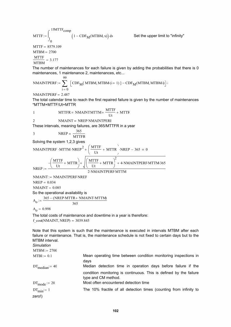
102

MTTF0

15MTTFcompx1 CDFM MTBM x,( )−( )

⌠⌡

d:= Set the upper limit to "infinity"

MTTF 8579.109=MTBM 2700=MTTFMTBM

3.177=

The number of maintenances for each failure is given by adding the probabilities that there is 0maintenances, 1 maintenance 2, maintenances, etc...

NMAINTPERF

0

99

i

CDFM MTBM MTBM i 1+( )⋅,[ ] CDFM MTBM MTBM i⋅,( )− i⋅∑=

:=

NMAINTPERF 2.487=The total calendar time to reach the first repaired failure is given by the number of maintenances*MTTM+MTTF/Ut+MTTR

1 MTTFR NMAINTMTTMMTTF

Ut+ MTTR+

2 NMAINT NREP NMAINTPERF⋅These intervals, meaning failures, are 365/MTTFR in a year

3 NREP365

MTTFRSolving the system 1,2,3 gives

NMAINTPERF MTTM⋅ NREP2⋅

MTTFUt

MTTR+

NREP⋅+ 365− 0

NREP

MTTFUt

MTTR+

−MTTF

UtMTTR+

24 NMAINTPERF⋅ MTTM⋅ 365⋅++

2 NMAINTPERF⋅ MTTM⋅:=

NMAINT NMAINTPERF NREP⋅:=NREP 0.034=NMAINT 0.085=So the operational availability is

Ao365 NREP MTTR⋅ NMAINT MTTM⋅+( )−

365:=

Ao 0.998=

The total costs of maintenance and downtime in a year is therefore:f_cost NMAINT NREP,( ) 3039.845=

Note that this system is such that the maintenance is executed in intervals MTBM after eachfailure or maintenance. That is, the maintenance schedule is not fixed to certain days but to theMTBM interval.SimulationMTBM 2700:=MTBI 0.1:= Mean operating time between condition monitoring inspections in

daysDTmedian 40:= Median detection time in operation days before failure if the

condition monitoring is continuous. This is defined by the failuretype and CM method.

DTmode 20:= Most often encountered detection time

DTmin 1:= The 10% fractile of all detection times (counting from infinity to

zero!)

103

DTmax 50:= The 90% fractile of all detection times (counting from infinity to

zero!)CINSP 0:= Cost of one inspectionDC 0.75:= Diagnostics coverage % of failures detectedMTTAM 15:= Mean operating time to arrange a maintenance break when a

failure has been diagnosed. This is in fact function of currentmachine reliability, the scheduled opportunity as well as availabilityof resources.

f_detectionpdf x α, λ,( ) dgamma x λ⋅ α,( ):=

f_detectioncdf x α, λ,( ) pgamma x λ⋅ α,( ):=

f_detection icdf p α, λ,( ) qgamma p α,( )λ

:=

LSQ α λ,( )0

rows t( ) 1−

i

f_detectioncdf ti α, λ,( ) Fi−( )2∑=

:=

Least Square Method for Curve Fittingα 1.1:=

λα 1−

DTmode:=

Givenα 0>λ 0>DTmode λ⋅ 1>

α 1− DTmode λ⋅

Fix the mode valueλ

α

Minimize LSQ λ, α,( ):=

λ 0.05=α 2=Detection density function

0 20 40 60 80 1000

0.5

1

f_detection pdf x α, λ,( )

x

F

0.10

0.50

0.90

:=t

DTmin

DTmedian

DTmax

:=

104

Detection icdf function - the failure prediction time as a function of probability, if the failure ispredicted at all.

0 0.2 0.4 0.6 0.8 10

50

100

f_detectionicdf p α, λ,( )

pThe effect of MTTAM to diagnostics coverage

1 f_detectioncdf MTTAM α, λ,( )−( ) DC⋅ 0.620=

f_detectioncdf MTTAM α, λ,( ) 0.173=

Simulation algorithm- Simulates events of failures and maintenance actions, st is the maximum simulation time

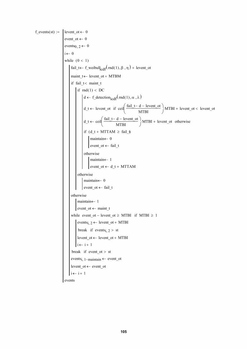
105

f_events st( ) levent_ot 0←

event_ot 0←

events0 2, 0←

i 0←

fail_t f_weibullicdf rnd 1( ) β, η,( ) levent_ot+←

maint_t levent_ot MTBM+←

d f_detectionicdf rnd 1( ) α, λ,( )←

d_t levent_ot← ceilfail_t d− levent_ot−

MTBI

MTBI⋅ levent_ot+ levent_ot<if

d_t ceilfail_t d− levent_ot−

MTBI

MTBI⋅ levent_ot+← otherwise

maintain 0←

event_ot fail_t←

d_t MTTAM+ fail_t≥( )if

maintain 1←

event_ot d_t MTTAM+←

otherwise

rnd 1( ) DC<if

maintain 0←

event_ot fail_t←

otherwise

fail_t maint_t<if

maintain 1←

event_ot maint_t←

otherwise

eventsi 2, levent_ot MTBI+←

break eventsi 2, st>if

levent_ot levent_ot MTBI+←

i i 1+←

event_ot levent_ot− MTBI≥while MTBI 1≥if

break event_ot st>if

eventsi 1 maintain−, event_ot←

levent_ot event_ot←

i i 1+←

0 1<( )while

events

:=

106

f_removenulls invector( ) outvector 0 0←

j 0←

outvector j invectori←

j j 1+←

invectori 0>if

i 0 rows invector( ) 1−..∈for

outvector

:=

f_intervals eventlist( ) j 0←

intervals0 0←

intervalsj eventlisti eventlisti 1−−← j 0>if

intervals0 eventlist0← otherwise

j j 1+←

i 0 rows eventlist( ) 1−..∈for

intervals

:=

Simulate 1000000 years of operation timen 1000000:=events f_events 365 n⋅( ):=Failures on the first column, maintenance on 2nd, and inspections on 3rd

eventsT0 1 2 3 4 5 6

012

2700 5400 8100 10800 12101.3 14345.9 17045.90 0 0 0 0 0 00 0 0 0 0 0 0

=

allevents events 0⟨ ⟩ events 1⟨ ⟩+:=total_ot max events( ):=allintervals sort f_intervals allevents( )( ):=Take the intervals between failure and maintenance eventscalendarevents calendarevents 0 0, 0←

calendarevents 0 1, 0←

lastDelay MTTM←

tmpEventsevents

Ut←

calendarevents i 0, tmpEventsi 0, lastDelay+←

lastDelay MTTM←

tmpEventsi 0, 0>if

calendarevents i 1, tmpEventsi 1, lastDelay+←

lastDelay MTTR←

otherwise

i 0 rows events( ) 1−..∈for

calendarevents

:=

allcalendarevents calendarevents0⟨ ⟩ calendarevents1⟨ ⟩+:=allcalendarintervals sort f_intervals allcalendarevents( )( ):=

repairtimes f_removenulls events 1⟨ ⟩( ):=repairintervals f_intervals repairtimes( ):=

mainttimes f_removenulls events 0⟨ ⟩( ):=

107

maintintervals f_intervals mainttimes( ):=All the event intervals, repair intervals and maintenance intervals

allintervalsT 0 1 2 3 4 5 6 7 8 90 14.529 15 15 15 34.2 39.6 42.3 50.2 54.1 54.3

=

repairintervalsT 0 1 2 3 4 50 22208.41 69259.229 24982.227 7982.06 30702.323 516.616

=

maintintervalsT 0 1 2 3 4 5 6 70 2700 2700 2700 2700 1301.3 2244.6 2700 2700

=

insptimes f_removenulls events 2⟨ ⟩( ):=The need for materials is defined by either maintenance or failuresµ all mean allintervals( ):=

σ all Stdev allintervals( ):=

µall 2457.378=

σall 493.992=

Confidence level 99%allintervals round rows allintervals( ) 1−( ) 0.99⋅[ ] 2700=

The values of repair and maintenance intervals are as followsThe mean operating time to failure of the function from last failureµr mean repairintervals( ):=

σ r Stdev repairintervals( ):=

medrep median repairintervals( ):=µr 22738.489=

σr 22284.381=

medrep 15796.737=The mean operating time to maintenance of the function from last maintenanceµm mean maintintervals( ):=

σm Stdev maintintervals( ):=

medmaint median maintintervals( ):=µm 2755.106=

σm 836.778=

medmaint 2700=Number of repairs and maintenancesNREP rows repairtimes( ):=NREP 16051=NMAINT rows mainttimes( ):=

NMAINT 1.325 105×=

NREP NMAINT+ 1.485 105×=

NMAINTNREP

8.254=

NINSP 0 MTBI 1<if

rows insptimes( ) otherwise

:=

NINSP 0=i 0 rows repairintervals( ) 1−..:=t sort repairintervals( ):=

pii

rows repairintervals( ):=

Failure probability function under condition monitoring and maintenance

108

0 5000 1 .104 1.5 .1040

0.5

1

CDF ti β, η,( )pi

tiThe total maintenance costs

TCTtotal_ot

UtNMAINT MTTM⋅+ NREP MTTR⋅+:=

Total simulated calendar time

TCT 4.57 108×=

NMAINTNMAINT

TCT365⋅:=

Number of maintenances in a year

NREPNREPTCT

365⋅:=

Number of repairs in a year

NINSPNINSP

TCT365⋅:=

NREP 0.013=NMAINT 0.106=NINSP 0=f_cost nmaint nrep, ninsp,( ) f_cost nmaint nrep,( ) ninsp CINSP⋅+:=Simulated costs of maintenancef_cost NMAINT NREP, NINSP,( ) 1958.778=Operational availability

Ao365 NREP MTTR⋅ NMAINT MTTM⋅+( )−

365:=

Ao 0.99837=

109

APPENDIX C: MODEL IV IN VENSIM 5.0TEXT FORMAT

Idle Workers= INTEG (Repair Worker DeallocationRate+Maintenance Worker DeallocationRate-Repair Worker Allocation Rate-CBMaintenance Worker Allocation Rate-PMWorker Allocation Rate, Number OfWorkers)

Number Of Workers= 30Total Lifetime of Components= INTEG (Components In Operation-

(Necessary CBM Work StartRate+Components Failing During WaitingRate+PM Work Start Rate+UndetectedFailure Rate+Unnecessary CBM WorkStart Rate)*Average Lifetime ofComponents,1)

Failure Rate2= MAX(Working Components To Be CBMaintained/1000*Statistical FailureDistribution(Average Lifetime ofComponents/Component MTTF),0)

Components In Operation= Components That Fail Soon+Componentsthat Fail in their Infant Life+WorkingComponents+Working Components To Be CBMaintained

Working Components To Be CB Maintained= INTEG (False Diagnostics alarmRate-Unnecessary CBM Work Start Rate-Failure Rate2,0)

Components That Fail Soon= INTEG (Failure Rate+Failure Rate2-Detected Failure Rate-UndetectedFailure Rate,0)

Difference= Y-Min Percentage of Operating andMaintained Components*1000

Y= 1000-Components Under Repair-FailedComponents Due to Aging-FailedComponents Due To Infant Failures

Total Failed Components= Failed Components Due To InfantFailures+Failed Components Due toAging

Integral Gain= 5Integral of Difference= INTEG (Difference,0)Failures= MAX(Working

Components/1000*Statistical FailureDistribution(Average Lifetime ofComponents/ComponentMTTF),0)*(1+STEP(0,2340))

Component MTTF= 520Repair Quality= Average Repair QualityRepair Work Start Rate 1= ZIDZ(Failed Components Due to

Aging,Total Failed Components)*RepairWork Start Rate

Renewal Delay= MAX(MIN(0.7*520+Integral Gain*Integralof Difference+Difference*CorrectionGain,520),208)

Failed Components Due To Infant Failures= INTEG (Infant Failure Rate-Repair Work Start Rate 2,0)

Components Under Repair= INTEG (Repair Work Start Rate 1+RepairWork Start Rate 2-Errorneus RepairRate-Quality Repair Rate, 0)

Required PM Start Rate= Working Components/Renewal Delay

110

Required Repair Start Rate= Total Failed Components/AdministrationDelay of A Worker

Repair Work Start Rate 2= ZIDZ(Failed Components Due To InfantFailures,Total FailedComponents)*Repair Work Start Rate

Failed Components Due to Aging= INTEG (Undetected FailureRate+Components Failing During WaitingRate-Repair Work Start Rate 1,0)

False Diagnostics Proportion= 0Components Under Maintenance= INTEG (Necessary CBM Work Start

Rate+Unnecessary CBM Work StartRate+PM Work Start Rate-QualityMaintenance Rate-ErrorneousMaintenance Rate, 0)

Maintenance Quality= Average Maintenance Quality+AverageMaintenance Quality*Noise

Average Repair Quality= 0.9Components Failing During Waiting Rate= Failing Components To Be CB

Maintained/(Failure Detection Time-Average Waiting of CB Components ToMaintenance)

Average Maintenance Quality= 0.95Noise= 0*0.025* SIN(Time*2*3.14159/Period)+

0*STEP(-0.05, 1560)+0*RANDOM NORMAL(-0.05, 0.05 , 0, 0.01, 0)

False Diagnostics alarm Rate= False Diagnostics Proportion*DetectedFailure Rate

Average Waiting of CB Components To Maintenance= ZIDZ(Total WaitingTime of Failing CB Components, FailingComponents To Be CB Maintained)

Failing Components To Be CB Maintained= INTEG (Detected Failure Rate-Necessary CBM Work Start Rate-Components Failing During WaitingRate, 0)

Total Components To Be CBM= Failing Components To Be CBMaintained+Working Components To Be CBMaintained

Unnecessary CBM Work Start Rate= ZIDZ(Working Components To Be CBMaintained,Total Components To BeCBM)*CBM Work Start Rate

Working Components= INTEG (Quality Repair Rate+QualityMaintenance Rate-Failure Rate-PM WorkStart Rate-False Diagnostics alarmRate,1000)

Required CB Maintenance Start Rate=Total Components To BeCBM/Administration Delay of A Worker

Total Waiting Time of Failing CB Components= INTEG (Failing ComponentsTo Be CB Maintained-(ComponentsFailing During Waiting Rate+NecessaryCBM Work Start Rate)*Average Waitingof CB Components To Maintenance, 1)

Necessary CBM Work Start Rate= ZIDZ(Failing Components To Be CBMaintained,Total Components To BeCBM)* CBM Work Start Rate

Period= 52Correction Gain= 50Average Maintenance Time= 4Min Percentage of Operating and Maintained Components= 0.997Failure Rate= FailuresAdministration Delay of A Worker=1Available CB Maintenance Start Rate= MAX(Available Repair Start Rate-

Repair Work Start Rate,0)

111

Available PM Start Rate= MAX(Available CB Maintenance StartRate-CBM Work Start Rate,0)

Available Repair Start Rate= Idle Workers/Worker Allocation PerComponent Failure/Administration Delayof A Worker

Maintenance Worker Deallocation Rate= Maintenance Workers/AverageMaintenance Time

Average Lifetime of Components= Total Lifetime ofComponents/Components In Operation

PM Worker Allocation Rate= PM Work Start Rate*Worker AllocationPer Maintenance

CBM Work Start Rate= MIN(Available CB Maintenance StartRate,Required CB Maintenance StartRate)

CB Maintenance Worker Allocation Rate= CBM Work Start Rate*WorkerAllocation Per Maintenance

PM Work Start Rate= MIN(Available PM Start Rate,RequiredPM Start Rate)

Repair Workers= INTEG (Repair Worker Allocation Rate-Repair Worker Deallocation Rate, 0)

Undetected Failure Rate= MAX(Components That Fail Soon*(1-Diagnostics Coverage)/Failure Time4,0)

Worker Allocation Per Maintenance= 1Repair Worker Deallocation Rate= Repair Workers/Average Repair TimeMaintenance Workers= INTEG (CB Maintenance Worker

Allocation Rate+PM Worker AllocationRate-Maintenance Worker DeallocationRate,0)

Repair Work Start Rate= MIN(Available Repair StartRate,Required Repair Start Rate)

Repair Worker Allocation Rate= Repair Work Start Rate*WorkerAllocation Per Component Failure

Worker Allocation Per Component Failure= 2Statistical Failure Distribution ([(0,0)-

(2,40)],(0,0),(0.1,0.001),(0.2,0.01),(0.3,0.051),(0.4,0.161),(0.5,0.392),(0.6,0.813),(0.7,1.507),(0.8,2.57),(0.9,4.117),(0.95,5.111),(1,6.274),(1.1,9.186),(1.3,17.921),(1.5,31.765))

Failure Detection Time= 8Average Infant Failure Time= 5Failure Time4= 12Average Repair Time= 3Quality Maintenance Rate= Components UnderMaintenance*Maintenance Quality/Average Maintenance TimeDetected Failure Rate= MAX(Components That Fail

Soon*Diagnostics Coverage/(FailureTime4-Failure Detection Time ),0)

Diagnostics Coverage= 0Errorneous Maintenance Rate= Components Under Maintenance*(1-

Maintenance Quality)/AverageMaintenance Time

Errorneus Repair Rate= Components Under Repair*(1-RepairQuality)/Average Repair Time

Infant Failure Rate= Components that Fail in their InfantLife/Average Infant Failure Time

Quality Repair Rate= Components Under Repair*RepairQuality/Average Repair Time

Components that Fail in their Infant Life= INTEG (ErrorneousMaintenance Rate+Errorneus RepairRate-Infant Failure Rate, 0)

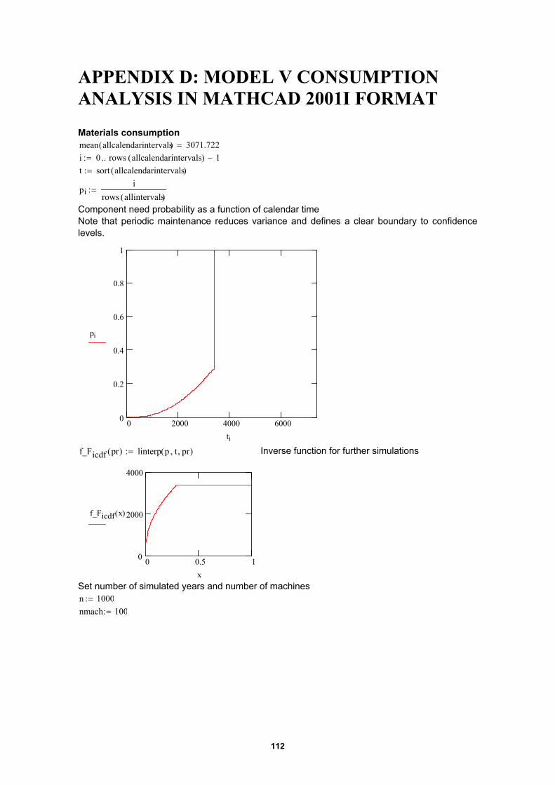
112

APPENDIX D: MODEL V CONSUMPTIONANALYSIS IN MATHCAD 2001I FORMAT

Materials consumptionmean allcalendarintervals( ) 3071.722=i 0 rows allcalendarintervals( ) 1−..:=t sort allcalendarintervals( ):=

pii

rows allintervals( ):=

Component need probability as a function of calendar timeNote that periodic maintenance reduces variance and defines a clear boundary to confidencelevels.

0 2000 4000 60000

0.2

0.4

0.6

0.8

1

pi

tif_Ficdf pr( ) linterp p t, pr,( ):= Inverse function for further simulations

0 0.5 10

2000

4000

f_Ficdf x( )

xSet number of simulated years and number of machinesn 1000:=nmach 100:=

113

f_simt max_t nmach, f_Ficdf,( ) prev_t 0←

i 0←

event_t 0←

event_t prev_t f_Ficdf rnd 1( )( )+←

break max_t event_t≤if

retAi event_t←

prev_t event_t←

i i 1+←

0 1<( )while

prev_t 0←

event_t 0←

k 0 nmach 1−..∈for

sort retA( )

:=

machgroupintervals f_intervals f_simt 365 n⋅ nmach, f_Ficdf,( )( ):=

machgroupintervalsT 0 1 2 3 4 5 6 7 80 339.367 119.386 512.221 28.059 6.716 37.593 419.122 11.186 31.426

=

µgroup mean machgroupintervals( ):=

σgroup stdev machgroupintervals( ):=

µgroup 30.827=

σgroup 32.14=

i 0 rows machgroupintervals( ) 1−..:=t sort machgroupintervals( ):=

tT 0 1 2 3 4 5 6 7 8 90 0 0 0 0 0 0 0 0 0 0

=

pii

rows machgroupintervals( ):=

pT 0 1 2 3 4 5 60 0 8.446·10 -5 0 0 0 0 0.001

=

Spare parts consumption interval cdf of a machine group

0 50 1000

0.2

0.4

0.6

0.8

1

pexp ti1

µgroup,

pi

ti

µgroup 30.827=

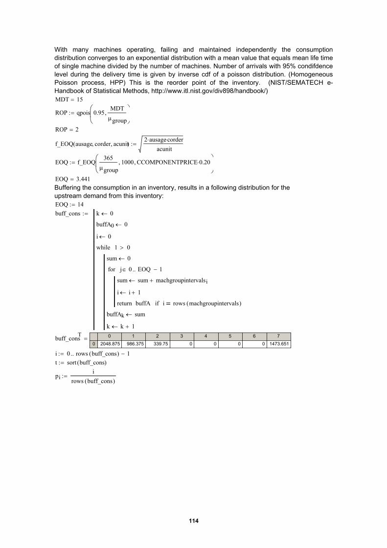
114

With many machines operating, failing and maintained independently the consumptiondistribution converges to an exponential distribution with a mean value that equals mean life timeof single machine divided by the number of machines. Number of arrivals with 95% condifdencelevel during the delivery time is given by inverse cdf of a poisson distribution. (HomogeneousPoisson process, HPP) This is the reorder point of the inventory. (NIST/SEMATECH e-Handbook of Statistical Methods, http://www.itl.nist.gov/div898/handbook/)MDT 15=

ROP qpois 0.95MDTµgroup,

:=

ROP 2=

f_EOQ ausage corder, acunit,( )2 ausage⋅ corder⋅

acunit:=

EOQ f_EOQ365

µgroup1000, CCOMPONENTPRICE 0.20⋅,

:=

EOQ 3.441=Buffering the consumption in an inventory, results in a following distribution for theupstream demand from this inventory:EOQ 14:=buff_cons k 0←

buffA0 0←

i 0←

sum 0←

sum sum machgroupintervalsi+←

i i 1+←

buffAreturn i rows machgroupintervals( )if

j 0 EOQ 1−..∈for

buffAk sum←

k k 1+←

1 0>while

:=

buff_consT 0 1 2 3 4 5 6 70 2048.875 986.375 339.75 0 0 0 0 1473.651

=

i 0 rows buff_cons( ) 1−..:=t sort buff_cons( ):=

pii

rows buff_cons( ):=

115

0 200 400 600 800 10000

0.2

0.4

0.6

0.8

1

pgammati

µgroupEOQ,

pi

pnorm ti EOQ µgroup⋅, EOQ µgroup⋅,( )

tiSpare parts orders distribution when the real consumption is buffered by EOQ. With EOQ=1, theconsumption follows exponential distribution, with EOQ>=1 the consumpiton follows Gammadistribution. With EOQ >> 1 the consumption can approximated with normal distribution(according to the central limit theorem) where mean is EOQ*mean of the exponential distributionand std. deviation is sqrt(EOQ)*mean of the exponential distribution.

116

APPENDIX E: MODEL V IN VENSIM 5.0TEXT FORMAT

Expected Demand2= SMOOTH3I( IF THEN ELSE(SharedInformation Status=0 :OR:RemoteMonitoring Status=0,Purhasing Plan3,Remote Monitoring),AveragingTimeframe2, Average Consumption)

Expected Demand3= SMOOTH3I( Consumption Rate, AveragingTimeframe3,Average Consumption )

Averaging Timeframe2= 35Averaging Timeframe3= 21Consumption Rate= RANDOM NORMAL(0, Average Consumption*6

, Average Consumption, 1*SQRT(AverageConsumption), 0)

Production Rate= DELAY3I(MIN(Production Plan,MaxCapacity),Production Delay, AverageConsumption)

Expected Demand1= SMOOTH3I(IF THEN ELSE(RemoteMonitoring Status=1, RemoteMonitoring, Purhasing Plan2),Averaging Timeframe1, AverageConsumption)

ShippingRate2to3= DELAY3I(IF THEN ELSE( Inventory2>0,Purhasing Plan3, 0), ShippingDelay2to3, Average Consumption)

Shipping Rate1to2= DELAY3I(IF THEN ELSE( Inventory1>0,Purhasing Plan2, 0), ShippingDelay1to2, Average Consumption)

Inventory Target1= Expected Demand1*(K*Production Delay)Average Consumption= 30+0*STEP(1.5,100)Inventory Correction Delay3= 14Demand Rate 3= IF THEN ELSE(Inventory3>0,ConsumptionRate,0)Inventory Correction Delay2= 28K= 2.5Inventory Target2= Expected Demand2*(ShippingDelay1to2*K)Inventory Target3= Expected Demand3*(ShippingDelay2to3*K)Shipping Delay2to3= 7Inventory3= INTEG (+ShippingRate2to3-Demand Rate

3,Average Consumption*(K*ShippingDelay2to3-Inventory CorrectionDelay3))

Purhasing Plan3= MAX((Inventory Target3-Inventory3)/Inventory CorrectionDelay3,0)

Remote Monitoring= Consumption RateRemote Monitoring Status= 0Production Delay= 21Production Plan= MAX(Inventory Target1-

Inventory1,0)/Production CorrectionDelay1

Purhasing Plan2= MAX((Inventory Target2-Inventory2)/Inventory CorrectionDelay2,0)

Shared Information Status= 0Shipping Delay1to2= 14Production Correction Delay1= 40

117

Inventory2= INTEG(+Shipping Rate1to2-ShippingRate2to3, AverageConsumption*(K*Shipping Delay1to2-Inventory Correction Delay2))

Max Capacity= 37.5Inventory1= INTEG (Production Rate-Shipping

Rate1to2, AverageConsumption*(K*Production Delay-Production Correction Delay1))

Averaging Timeframe1= 56

Helsinki University of TechnologyInformation and Computer Systems in Automation

Report 1 Koskinen, K., Aarnio, P. (eds.),Internet-, Intranet- and Multimedia Applications in Automation. June 1998.

Report 2 Koskinen, K., Aarnio, P. (eds.),PC-based Automation Systems and Applications. June 1999.

Report 3 Mattila MProsessilaitteen etätukijärjestelmä – ohjelmistoarkitehtuuri ja ohjelmistotekniset ratkaisut, March 2000

Report 4 Strömman MOhjelmoitavan logiikan ohjelmointi ohjelmistotuotantoprosessina, March 2002

Report 5 Aarnio PSimulation of a hybrid locomotion robot vehicle, June 2002

Report 6 Peltola JUudet automaatiojärjestelmät - komponenttipohjaisen automaatiosovelluksen suoritusympäristö, September2002

Report 7 Fortu TomEnterprise Resource Planning - Integration with Automation Systems, September 2002

Report 8 Mattila MCondition Monitoring of an X-ray Analyzer, February 2003

Report 9 Sierla SMiddleware solutions for automation applications - case RTPS, June 2003

Report 10 Honkanen TModelling Industrial Maintenance Systems and the Effects of Automatic Condition Monitoring, February 2004

ISBN 951-22-6815-9ISBN 951-22-6816-7 (PDF)ISSN 1456-0887