MODELING WELFARE LOSS ASYMMETRIES ARISING FROM

UNCERTAINTY IN THE REGULATORY COST OF FINANCE

Ian M Dobbs

Newcastle University Business School

Newcastle University

JEL Classification: C15, L51, L97.

Keywords: Allowed rate of return, Price Cap, Regulation, Simulation, WACC, Welfare

loss.

2

ABSTRACT

The allowed rate of return (AROR) is a critical input in the regulatory assessment of

revenue requirements, price caps and other controls. Errors in estimating AROR impact

on investment incentives and price setting and hence can induce welfare loss. It is often

suggested that the welfare losses that arise from under-estimation of the AROR may be

significantly greater than arise from over-estimation. However, to date, this proposition

has not been examined in any detail. This paper assesses the extent of welfare loss

asymmetry and its implications for the choice of AROR.

3

1. Introduction

The allowed rate of return (AROR) is a critical input when setting price caps and controls.

Regulators typically base the AROR on their view of the firm’s weighted average cost of

capital, the ‘WACC’ (see e.g. Brennan and Schwartz [1982]). This paper focuses on the

consequences of uncertainty in WACC estimation for the regulator’s choice of AROR. It

has often been argued by regulators and consultants that the welfare losses arising from

‘under-investment’ when setting too low an AROR are likely to be greater than from

some degree of ‘over-pricing’ when setting it ‘too high’, and that this motivates setting an

AROR above the mean value of the WACC distribution.1 The qualitative argument is that

the welfare impact of ‘too low’ an AROR on investment is likely to be significantly

greater than the impact of ‘over-pricing’ if it is set ‘too high’. However, whilst this may

be plausible, there has been little work done to date on the likely quantitative impact, and

hence an attendant difficulty in deciding on the extent of ‘uplift’ required in AROR. 2

The only contribution to attempt an explicit analysis appears to be a report submitted by

Wright, Mason and Miles [2003] to the UK Department of Trade and Industry and the

Competition Commission; chapter 5 of that report discusses a single period ‘now or

never’ or ‘non-deferrable’ investment, and the consequences of errors in estimation of the

cost of finance (the latter modeled via a uniform distribution). In this simple model, if

the actual cost of finance turns out to be higher than the allowed rate of return, the

investment is not undertaken and there is neither profit to the firm nor consumer surplus;

only if the cost of finance turns out to be less than the AROR is the project undertaken.

The present paper can be viewed as a significant extension of this exploratory work in

that it examines long lived investments within the context of a sequence of regulatory

1 Regulators who have accepted the argument include Ofcom [2005], CAA [2007], the Competition Commission [2007], NZCC [2004], and ACCC [2005]. Various consultancy reports suggest the use of higher percentiles of the WACC distribution (the 75th , 85th, even 95th): See Bowman [2004, 2005], SFG [2005], PWC [2006] and Dobbs [2008]. 2 Other sources for potential error in valuation include uncertainty concerning the scope for cost reductions through technical progress and learning by doing, uncertainty concerning developments in the level of future demand and so on. Whilst these other sources of uncertainty may also be important, it is worth noting that uncertainty over financing costs, the focus of the present work, is pervasive.

4

review periods, it allows a general distribution for the WACC, and considers already sunk

investments and deferrable investments in addition to non-deferrable investments (it can

be argued that the non-deferrable case is the least important category empirically, since

most new investment is in fact deferrable).

The basic framework involves the regulator setting an AROR and then determining price

controls which hold throughout a fixed regulatory review period (RRP).3 The price

controls aim to allow a revenue stream that will just compensate the firm for the costs it

incurs, including the cost of capital (see Leland [1974], Brennan and Schwartz [1982],

Guthrie [2006]). The actual cost of finance subsequently faced by the firm is uncertain

and may thus deviate from the AROR set by the regulator. This means that the firm, once

it knows its cost of finance, can decide on whether to invest or not, and where

investments are deferrable, it may choose to defer the decision to the next RRP.

However, once a service is launched, a ‘universal service obligation’ applies, such that

the firm is required to satisfy the demand for the service through all future time (see

Evans and Guthrie [2005]).

It is shown that for sunk investment, there is little argument for up-lift in AROR, whilst

for both new non-deferrable and new deferrable investment, there is a strong case for

uplift in AROR. This is for two reasons; firstly, because the AROR that maximizes

economic welfare is likely to be well in excess of the mean of the WACC distribution, and

secondly, because there is inevitably uncertainty over the exact location of the optimum,

and the errors that arise from setting the AROR too high are much less than those

associated with setting it too low. When price cap regulation is applied to a mix of the

old and the new, it is further shown that even a quite small component of new investment

can motivate a significant increase in the AROR.

Before proceeding, it is perhaps worth emphasizing that the argument that the AROR

should be set above the expected value of the WACC distribution arises from two key

3 This is standard practice for incentive regulation regimes. By contrast, rate of return regulation typically featured endogenous timing for the RRP, wherein either the regulator or the regulatee could initiate a request for a regulatory hearing (see Guthrie [2006]).

5

‘second best’ features. Firstly, the assumption that the firm has control over new

investment and its timing, and secondly, the assumption that the AROR and the associated

price caps and controls are fixed for the duration of the regulatory review period (RRP).

The strength of the argument might be somewhat mitigated through the use of AROR

adjustment triggers, so long as these feed through into price (cap) adjustments within the

RRP. 4 Such an approach has not yet found any regulatory favor, perhaps because price

uncertainty and tariff adjustment costs impact on both consumers and the firm.

Alternatively, incentives for new investment might be tackled on a project specific basis,

through assessments of likely impacts of real option effects or through adjustments to

assumptions concerning future cash flows. However this is a long way from ‘light touch

regulation’ as it would involve detailed second guessing of the circumstances surrounding

each and every project specific proposal. It can be argued that building incentivization

into the assessment of the AROR for each given class of investment is a relatively light

touch approach and one which offers perhaps the simplest and clearest signal to the firm.

Accordingly, the above alternatives are not considered further in what follows.

In what follows, section 2 presents the basic analytic framework and establishes solutions

for the allowed rate of return for the three categories of investment. Section 3 then

presents numerical solutions and sensitivity analysis. Section 4 examines robustness to

variations in the model specification and section 5 concludes

2. The Analytic Framework

Three categories of investment are examined: category 1 is existing business (an already

sunk investment); category 2 is new investment that can be undertaken, if at all, only in

the up-coming regulatory review period (RRP); category 3 is investment which can be

implemented in the RRP – or which can be deferred to a future RRP. In most cases, given

the relatively short period of regulatory review (typically 5 years or less – and rarely

4 Just as airlines implement price adjustments based on a ‘fuel price adjustment clause’, this would involve a ‘trigger’ that adjusts the AROR, contingent on events such as changes in the underlying level for the risk free rate of interest. See First Economics [2007] and Brealey and Franks [2009] for a discussion of the pros and cons of such schemes.

6

more than 7 years), a large part of the business is likely to be category 1 investment,

followed by category 3. However, category 2 investment is included as a useful

benchmark and starting point for formal analysis.

The base model assumes investment features a constant physical depreciation rate, a

constant rate of expected demand growth, a constant elasticity of demand, no technical

progress, and where investment can be deferred, no risk that the option will expire at a

later date. Common knowledge is assumed by both the regulator and regulatee

concerning these parameters.5 The robustness of results to variations in assumptions is

discussed in section 4 below. In particular, extensions to the case where there are

economies of scale in investment and where there is the possibility that options expire are

explored.

For the ith category of investment, ic denotes marginal operating cost; ik , per unit

capacity cost6; iε , demand elasticity; iγ , the rate of physical depreciation; and iα , the rate

of demand growth. It is assumed that if there is falling demand over time ( 0iα < ), it falls

at a rate less than that of physical depreciation (such that 0α γ+ > ), so there is

continuing demand for investment, and that demand is elastic ( 1iε < − ).7 The demand

curve at time t is

i itit i itq B e pα ε= . (1)

Since each category of investment is dealt with separately, to reduce unnecessary

notational clutter, the ‘i’ subscript is omitted where this does not affect intelligibility.

The sequence of decisions is as follows:

1. Time 0 – The regulator sets the AROR, r̂ and calculates the price cap, p̂ for each category of investment. The actual cost of finance r is then drawn

5 See Lewis and Sappington [1988]. The only source of asymmetric information in the present model arises from the fact that, after the regulatory price cap determination, the cost of finance becomes known to the firm cf. Baron and Myerson [1982]. 6 Assumed constant in the benchmark model - the effect of allowing economies of scale are analyzed in section 4. 7 With constant elasticity demand, this ensures consumer surplus is finite in the subsequent welfare analysis.

7

from a fixed distribution with known density function ( )rφ on support [ , ]l ur r .

2. Time 0 – For category 1 (sunk) investment, the firm has no decision to take.

Investment is required to service demand and cover physical depreciation. For category 2 (non-deferrable) investment, the firm chooses to accept or reject the opportunity. If accepted, the firm must service demand over time at the set price. For category 3 (deferrable) investment, the firm chooses to accept now, or takes the option to defer to the next regulatory review period. Again, if accepted, the firm is required to service demand over time at the set price.

3. Time T, 2T, 3T… – The regulatory cycle repeats. For category 3

investment, if it was deferred at the previous RRP, then, if the investment opportunity still exists,8 the decision on whether to invest is reconsidered again.

The firm’s WACC, denoted r, is a random variable with known density function ( )rφ

assumed invariant from one RRP to the next.9 The regulator knows this distribution, and

sets a fixed AROR, denoted r̂ , and then price caps, p̂ so as to reduce project value to

zero (i.e. to just break even). Given stationarity, there is no reason for the regulator to set

anything other than a time invariant price cap. At the next RRP, all new investment made

in previous RRPs becomes category 1 sunk investment. For simplicity, in the above

specification, the uncertainty in r is resolved immediately after the price caps are set, with

the decision to defer only available to the beginning of each RRP.10

No distinction is drawn between private and social rates of time preference and it is also

assumed that the different categories of investment can be valued at the firm’s cost of

capital. There are, of course, many examples of a regulator distinguishing the level of

8 The case where the opportunity only exists with a fixed probability is examined in section 4. The solution naturally converges on that for category 2 investment as the probability 0ρ → . 9 The distribution for r can be derived using Monte Carlo simulation, based on assumptions concerning the processes that generate the underlying WACC components (see e.g. NZCC [2004], ACCC[2005], Bowman [2004, 2005], SFG [2005], Competition Commission [2007]). 10 A more general formulation would involve the cost of finance evolving as a stochastic process and the possibility of projects being deferred within RRPs as well as across RRPs. Gaming issues or commitment problems are not addressed (notably, the problem that, once investment is sunk, the regulator has an incentive to reneg on the regulatory compact). See e.g. Besanko and Spulber [1992]. Newbery [1999],gives a useful review of the issues that can arise. The reasons why the regulator chooses to commit to a fixed AROR and fixed price caps ex ante (with no subsequent adjustment) also lie outside the model.

8

risk, and hence the cost of finance, by line of business (LOB); in the UK, Ofcom [2005]

does this for BT, as does the CAA [2007] in its recent determination of financing costs

for Heathrow and Gatwick airports. However, a mix of investment types still remains

within each LOB, and the analysis presented in this paper can be viewed as applying to

each LOB separately. The welfare measure used in what follows is the unweighted

discounted sum of firm profits and consumers surplus, where the actual cost of finance r

is used as the discount rate.

Closed form solutions are not available for the optimization problems faced by the firm

or the regulator, even if ( )rφ is assumed to take a simple form (such as the uniform

distribution). A numerical optimization approach is therefore adopted, based on a

simulation. 11 In recent years, regulators and other interested parties have often utilized

the simulation approach for establishing the WACC distribution; whatever the details of

the model used for the WACC, the ultimate outcome under the simulation approach is an

empirical frequency distribution for r. That is, the simulation generates a set of drawings

for the cost of finance ( ), 1,..,r j j n= where n is chosen to be a large enough number to

ensure stability of relevant statistics (such as the percentiles of the distribution).12

2.1 Category 2: Non deferrable New Investment

This type of investment is likely to be of less importance than category 1 and category 3

investments, simply because new investment is rarely a ‘now or never’ decision - there is

usually an option to defer. However, it is useful to start here as it facilitates the

somewhat more complex analysis of category 3 deferrable investment. This category 2

non-deferrable investment is similar in spirit to the exploratory work undertaken in

Wright et al [2003]. The principle difference lies in the fact that this earlier work dealt

only with a single RRP and a single period new ‘now or never’ investment problem. In

the present model, there is an infinite program of ongoing investment (if the firm chooses 11 The ‘neoclassical’ economics approach typically works with minimal qualitative structure. The value of such an approach is limited when the trade offs cannot be qualitatively signed (as here). In such circumstances, a computational approach can help to provide quantitative appreciation on how things interact (see Judd [1999]). 12 In fact 610n = is used; for the base case, this gives percentiles with standard errors of around 0.005% for the 1st and 99th, and of generally less than 0.003% in between.

9

to instigate the project) with possible growth in demand and physical depreciation. There

is, in addition, an infinite sequence of RRPs and uncertainty concerning the cost of

finance in future RRPs. Finally, both sunk and deferrable investments are examined in

addition to non-deferrable category (since the latter is, empirically, the least substantive

category).

The firm invests only if it calculates NPV>0. Given price is fixed at p̂ , demand13 is

ˆttq Be pα ε= . (2)

where the constant B determines the level of demand and α denotes the rate of growth in

demand. Thus initial capacity 0 ˆQ Bpε= is required. With new investment in capacity at

time t, denoted tI , the growth in capacity is t t tQ I Qγ= − . Since capacity at time t must

equal demand, it has to grow at the rate t tQ Qα= . Hence

( )t tI Qα γ= + . (3)

That is, instantaneous investment covers depreciation of existing stock and the addition of

new stock in order to satisfy demand at the regulated price.

Instantaneous profit at time t is

( )( )ˆ ˆ( ) ( )

ˆ ˆ( )t t t t

tp c q kI p c k q

p c k Be pα επ α γ

α γ= − − = − − += − − + . (4)

Value from the regulator’s perspective is then

( ) ( )ˆˆ0 00 0

ˆ ˆ ( )ˆ ( )ˆ

ˆ

r trttV e dt kQ Bp p c k e dt kQ

p c kBp kr

αε

ε

π α γα γα

∞ ∞ −−= − = − − + − =− − +⎛ ⎞= −⎜ ⎟−⎝ ⎠

∫ ∫ . (5)

For simplicity, parameter ranges are set such that regulatory price caps are always

binding (that is, the unconstrained monopoly price is never below the price cap). The

regulator uses r̂ as the discount rate and aims to choose the price p̂ so as to reduce

discounted profit over the project life to zero; given (5), this implies choosing p̂ so that

13 The riskiness of the future cash flows in not explicitly modeled. Demand is best interpreted as ‘expected demand’, with the ‘cost of finance’, r, being the appropriate cost of finance for cash flows of this level of ‘riskiness’.

10

ˆ ( ) 0ˆ

p c k krα γα

− − +⎛ ⎞− =⎜ ⎟−⎝ ⎠, (6)

so

( )ˆ ˆ ˆ( ) ( )p c k r k c r kα γ α γ= + + + − = + + . (7)

The price is thus set to long run marginal cost, based on the regulator’s view of what

constitutes an appropriate cost of finance, r̂ .

The actual cost of finance, r which holds on (0,T) is now drawn (the cost of finance on

the second and subsequent RRPs remain random variables from the perspective of the

firm). In view of (7), (4) can be written as

( )ˆ ˆ ( )

ˆ ˆ( )

tt

tBp p c k eBp r ke

ε α

ε απ α γ

α= − − += − for [0, )t∈ ∞ . (8)

Denote initial profitability as

0 ˆ ˆ( )Bp r kεπ α= − . (9)

Then, value from the firm’s perspective can be written as

( ) ( )0 0 2 20 0

( 1) ( )0 0

( ) ( )0 0 00 0

( )

.. ( ) ...

( )

u

lu

lu

l

T T rr t rT r tf r

m T rrT r tm mmT r

T rr t rT r t

r

V e dt e e r dr dt

e e r dr dt kQ

e dt e e r drdt kQ

α α

α

α α

π π φ

π φ

π π φ

− − −

+− −

∞− − −

= +

+ + + −

= + −

∫ ∫ ∫∫ ∫

∫ ∫ ∫ . (10)

The first line of (10) emphasizes that value to the firm is the discounted profits on (0,T)

based on the realized discount rate r, plus the discounted profits on each subsequent RRP,

each of which depends on what the cost of finance is in that period. Viewed from time

zero, the cost of finance r in the second and subsequent RRP’s are independent random

variables, denoted as , 2,3,...tr t = in (10). The second term in the last line of (10) can be

written as:

( ) 1( )

0( ) ( )u u

l l

r rr t

r re r drdt r r drα φ α φ

∞ −− = −∫ ∫ ∫ . (11)

It proves useful to define an ‘expected discount rate’, denoted edr , that satisfies

( ) ( )1 1 ( )u

l

r

ed rr r r drα α φ− −− = −∫ . (12)

11

This can be solved for edr , given the RHS can be estimated numerically as

( ) ( )11

1( ) (1/ ) ( )u

l

r n

irr r dr n r iα φ α

−−

=− ≈ −∑∫ . (13)

(recall the Monte Carlo simulation involves n runs, with ( )r j denoting the WACC that

resulted from the jth simulation run). Note that edr depends on α 14 and that ( )edr E r< ;15

this follows from Jensen’s inequality, since ( ) 1r α −− is a convex function of r . 16 The

value to the firm, ( )fV r , conditional on the realized value r in the first RRP, can now be

written as

( ) ( )0 0 00 0

( ) ( )

0 0

( ) ( )

1

u

l

T rr t rT r tf r

r T r T

ed

V r e dt e e r drdt kQ

e e kQr r

α α

α α

π π φ

πα α

∞− − −

− −

= + −

⎧ ⎫−= + −⎨ ⎬− −⎩ ⎭

∫ ∫ ∫. (14)

Define the present value factor as

( ) ( )1( )

r T r T

ed

e eA rr r

α α

α α

− −⎧ ⎫−≡ +⎨ ⎬− −⎩ ⎭

. (15)

and note that 0 ˆQ Bpε= . So

[ ]( ) ( )

0 01 ˆ ˆ( ) ( )( ) 1

r T r T

fed

e eV r kQ Bp k A r rr r

α αεπ α

α α

− −⎧ ⎫−= + − = − −⎨ ⎬

− −⎩ ⎭. (16)

Thus the firm will only invest if value ( )fV r is positive (for this ‘all or nothing’ project).

That is, from (16), if

ˆ( )( ) 1 0A r r α− − > . (17)

Given an estimate for edr from (12), equation (17) can be numerically solved to find the

critical interest rate, denoted ar , which will induce investment. That is, investment occurs

if

14 To ensure convergence, values considered for the parameter α are restricted to satisfy lrα < , so that

( )( )iMin r iα < . 15 Given the assumption that ( )( )iMin r iα < , empirically, the effect is small – that is, edr is close to

( )E r . 16 The impact of uncertainty on discount factors is studied in Butler and Schachter [1989].

12

ar r< , (18)

and not otherwise, where ar is the solution to

ˆ( )( ) 1 0aA r r α− − = . (19)

Note that, as T →∞ , so ( ) 1( )A r r α −→ − , and ˆar r→ , and the firm invests only if

ˆr r< . However, in practice, T is finite, and it can be shown in this case that ˆar r> and

that ar is an increasing function of r̂ ; the higher the AROR, the higher the threshold for r

above which investment ceases.

Consumer surplus at time t is

1 1ˆˆ ˆ

ˆ( ) ( 1) ( 1)t t t

pp pCS q p dp Be p dp Be p Be pα ε α ε α εε ε

∞ ∞ ∞+ +⎡ ⎤= = = + = − +⎣ ⎦∫ ∫ , (20)

so, adding this to instantaneous profit, instantaneous economic welfare can be written as

( ) ( ) ( )( )( )

1ˆ ˆ ˆ( 1)

ˆ ˆ1

t tt

t

w Be p Be p p c k

Be p p c k

α ε α ε

α ε

ε α γε α γ

ε

+ ⎡ ⎤= − + + − − +⎣ ⎦⎧ ⎫= − − +⎨ ⎬+⎩ ⎭

, (21)

if there is investment; that is, if ar r< (and zero otherwise). Note that tw does not

depend on r, although it does depend on r̂ via p̂ .

Writing initial instantaneous welfare as

( )0 ˆ ˆ1

w Bp p c kε ε α γε

⎧ ⎫= − − +⎨ ⎬+⎩ ⎭, (22)

so that 0t

tw w eα= , the net present value for welfare, for a given realization r in the first

RRP is

( ) ( )0 0 00 0

( ) ( )

0 0 0 0

ˆ( , ) ( )

1 ( )

u

l

T rr t rT r t

rr T r T

ed

W r r w e dt e w e r drdt kQ

e e w kQ A r w kQr r

α α

α α

φ

α α

∞− − −

− −

= + −

⎧ ⎫−= + − = −⎨ ⎬− −⎩ ⎭

∫ ∫ ∫ (23)

when investment occurs (and zero when it does not). Welfare W is written as ˆ( , )W r r in

(23) to emphasize the fact that it is a function of both the realized cost of finance r, and

also the AROR, r̂ ; the latter dependency arises because both 0 0,w Q in (23) depend on p̂

13

which in turn depends on r̂ through (7). Thus, expected NPV welfare, denoted 2EW , is

given as

ˆ( )

2 ˆ( , ) ( )a

l

r r

rEW W r r r drφ= ∫ , (24)

where ˆ( )ar r is implicitly defined by (19).

To summarize: The regulator first chooses r̂ . Given this discount rate, the regulator

then calculates the price cap p̂ that reduces its view of project value to zero. The firm

then observes the actual cost of finance r and decides whether to undertake the

investment. It does so if the realized return r is below the threshold rate ˆ( )ar r . Only if

ˆ( )ar r r< does the firm view the project as having positive value, and only if it undertakes

the investment is there any economic welfare gained from it. One can now ask the

question – what choice of AROR would actually maximize expected economic welfare?

This is denoted 2̂ *r (the subscript identifying the category of investment under

consideration) and is the solution to the problem ˆ( )

ˆ2̂ ˆ* arg max ( , ) ( )a

l

r r

r rr W r r r drφ= ∫ . (25)

Mathematically, the solution can be shown to lie anywhere in the interval [ , ]l ur r (see

appendix). However, unless demand is very elastic, the solution will lie above the mean

of the WACC distribution, and usually significantly above it. With some algebraic effort,

it can be shown that 2 2ˆ ˆ( , ) / 0, ( , ) / 0W r r r W r r r∂ ∂ < ∂ ∂ > and that ˆ ˆ( , ) / 0W r r r >∂ ∂ < as

ˆ( )ar r r>< (proof omitted). So, for ˆ( )ar r r< , W is positive, decreasing, and convex in r,

whilst for ˆ( )ar r r> , the firm chooses not to invest and the welfare contribution is zero.

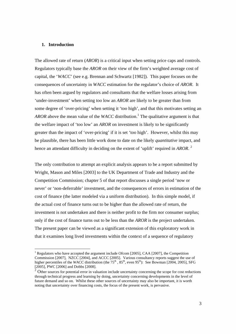
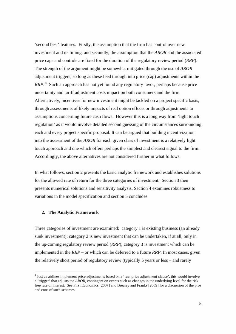
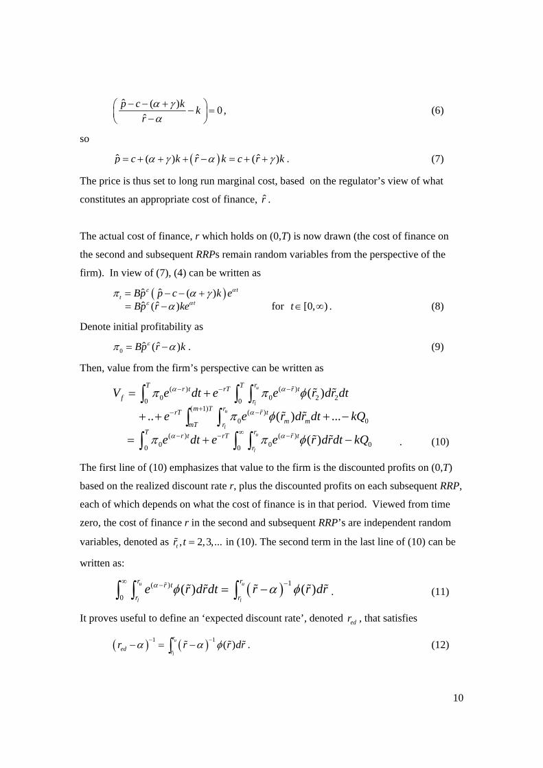
Figure 1 illustrates the function ˆ( , )W r r , and shows how there are two opposing forces

affecting 2EW ; firstly, an increase in r̂ increases ˆ( )ar r and this increases the range of r

on which projects are accepted (and hence adds economic welfare); secondly, the

increase in r̂ increases the price cap and so increases price above the socially optimal

level, resulting in a decrease in economic welfare at all levels of r, given that ˆ( )ar r r< .

14

Clearly, at low values for r̂ and hence lower values for ˆ( )ar r , it is the welfare gain from

increasing investment that dominates; as r̂ and hence ˆ( )ar r is increased, this is

eventually balanced by welfare losses arising from ‘over pricing’ as the price cap is

relaxed.

Figure 1: The ˆ( , )W r r function:

Effect of an increase in r̂ leading to an increase in ˆ( )ar r

+

-W(r,r)^

ra(r )^ r

Accept Reject

rl ru

Expected economic welfare 2EW can be evaluated numerically. The simulation

generates n realizations for r; the calculation of (24) is thus given simply as

( )2 ˆ. . ( ) ( )ˆ(1/ ) ( ),

ai s t r i r rEW n W r i r

∀ <≈ ∑ . (26)

Numerically, the optimization in (25) is achieved by setting r̂ equal to each of the

percentiles of the WACC distribution and selecting the percentile value that yields a

maximum value for 2EW .

15

2.2 Category 3: Deferrable Investment

The price cap is set as in (7). Once r is known, the firm accepts or defers the project to

the next RRP. The optimal decision rule involves setting a ‘critical value’, denoted cr ,

such that investment is accepted if cr r≤ and deferred if cr r> . The firm’s objective is to

choose cr to maximize expected firm value. Denote this expected value, prior to the

drawing for r, as EV. If the firm defers to the next regulatory review, given the stationary

environment, the expected value at that time is again EV. Writing EV as a function of cr

this implies

( ) ( ) ( ) ( ) ( )c u

l c

r r rTc f cr r

EV r V r r dr e EV r r drφ φ−= +∫ ∫ . (27)

Firm value ( )fV r is given by (16), so the first integral represents the expected value

contribution when investment is undertaken in the first RRP (when cr r≤ ). The second

integral represents the expected value contribution when investment is deferred (when

cr r> ). Re-arranging (27),

{ }( ) ( ) ( ) 1 ( )c u

l c

r r rTc fr r

EV r V r r dr e r drφ φ−= −∫ ∫ . (28)

The optimal strategy is to maximize (28) with respect to the choice variable cr . The

optimal choice for cr is

{ }* arg max ( ) ( ) 1 ( )c u

cl c

r r rTc r fr r

r V r r dr e r drφ φ−= −∫ ∫ . (29)

Computationally, this optimization can be achieved as part of the Monte Carlo

simulation. In the current implementation, it is optimized accurate to the nearest

percentile value of the WACC distribution. That is, setting cr to each percentile value of

the WACC distribution, equation (28) is evaluated and the solution is the percentile value

that gives maximum expected value. The key elements in (28) to be evaluated are:

( ). . ( )ˆ ˆ( ) ( ) (1/ ) ( ) ( ) 1c

cl

r

f i s t r i rrV r r dr n Bp k A r i rεφ α

∀ <≈ − −⎡ ⎤⎣ ⎦∑∫ (30)

and

16

( )

. . ( )( ) (1/ )u

cc

r rT r i Ti s t r i rr

e r dr n eφ− −∀ ≥

≈ ∑∫ . (31)

The optimal solution for *cr is an increasing function of r̂ such that ˆ ˆ*( )cr r r> .

Expected economic welfare for this category 3 investment, denoted by 3EW , is

{ }ˆ*( )

3 ˆ*( )ˆ ˆ( ) ( , ) ( ) 1 ( )c u

l c

r r r rT

r r rEW r W r r r dr e r drφ φ−= −∫ ∫ , (32)

where ˆ( , )W r r is given by (23).

The denominator in (32) is determined as per (31) and the numerator as

( )ˆ*( )

ˆ. . ( ) *( )ˆ ˆ( , ) ( ) (1/ ) ( ),c

cl

r r

i s t r i r rrW r r r dr n W r i rφ

∀ <≈ ∑∫ . (33)

Thus 3EW can be evaluated numerically for any given value set for r̂ . The optimal

choice for AROR for this category 3 investment is thus

{ }ˆ*( )

ˆ3 ˆ*( )ˆ ˆ* arg max ( , ) ( ) 1 ( )c u

l c

r r r rTr r r r

r W r r r dr e r drφ φ−= −∫ ∫ . (34)

The optimization (accurate to the nearest WACC percentile value) is found by setting r̂ to

each WACC percentile value in turn and evaluating (32), the optimum being that which

yields the maximum value.

The trigger value ˆ*( )cr r for category 3 is naturally lower than the trigger value ˆ( )ar r for

category 2. That is, the cost of finance r has to be even lower for it to be viewed as worth

investing and not deferring.17 However, note that for category 3 investment, and in

contrast to category 2, economic welfare is not completely lost when r is less than the

trigger level that induces investment, since although the investment is deferred, it is not

abandoned ‘for ever’.

17 This option value effect has long been recognized; see e.g. McDonald and Siegel [1986], Pindyck [1988], Dixit and Pindyck [1994], and in the context of regulatory price caps, Dobbs [2004].

17

2.3 Category 1: Existing capacity

Denote the level of existing capacity as eQ . For a given regulated price p̂ , it is possible

that this is above or below the initially required level of capacity, 0 ˆQ Bpε= . If 0eQ Q< ,

this means that an initial pulse of investment is required, followed by ongoing investment

to cover depreciation in existing assets and future demand growth.18 The alternative

possibility is that there is excess installed capacity at time 0. In this case, there is an

interval on which there is zero investment when price is set at short run marginal cost,

followed by an interval in which the regulated price rises in order to choke demand to

existing capacity, until a time is reached at which price reaches long run marginal cost,

and new investment commences. It is possible, but rather intricate, to model this. In any

case, the firm is a going concern and given the service obligation, will have had to meet

demand at the regulated price in the past, so it is not unreasonable to assume that existing

capacity eQ is well adjusted, such that 0eQ Q≈ . The solution for the case where 0eQ Q=

is in fact the same as that when 0eQ Q< so in what follows it is assumed that 0eQ Q≤ .

The analysis parallels that for category 2 investment, although the key difference is that

existing capacity eQ is already sunk.

The long run marginal cost regulated price p̂ applies, as in (7); economic welfare is then

similar to that in (23) except that part of capacity, eQ , is already sunk. Initial investment

in capacity is 0 eQ Q− . Thus economic welfare conditional on the value of r in the first

RRP is

( )

( )

( ) ( )1 0 0 00 0

( ) ( )

0 0 0 0

ˆ( , ) ( )

1 ( )

u

l

T rr t rT r ter

r T r T

e eed

W r r w e dt e w e r drdt k Q Q

e e w k Q Q A r w kQ kQr r

α α

α α

φ

α α

∞− − −

− −

= + − −

⎧ ⎫−= + − − = − +⎨ ⎬− −⎩ ⎭

∫ ∫ ∫ (35)

(recall 1 ˆ( , )W r r is a function of r̂ because both 0w and 0Q are functions of r̂ ). This

equation applies for all realizations [ ],l ur r r∈ . Thus

18 Recall that it is assumed that even if demand growth is negative, the rate of depreciation of physical capacity is assumed to be greater, so there is continuing need for investment over time.

18

1 1 ˆ( , ) ( )u

l

r

rEW W r r r drφ= ∫ . (36)

Optimal AROR for this category 1 investment is then given as

ˆ1 1ˆ ˆ* arg max ( , ) ( )u

l

r

r rr W r r r drφ= ∫ (37)

Notice that the term ekQ in (35) is a constant, and so has no effect on the optimization

(when choosing the best value for the AROR). That is, no specific choice for eQ is

required and, without loss of generality, it can be set to zero when conducting the ensuing

analysis. The numerical calculation of 1EW is simply

( )1 11ˆ(1/ ) ( ),n

iEW n W r i r

=≈ ∑ (38)

It can be shown mathematically that the optimal value for r̂ for this category lies below

the mean value of the WACC distribution, although empirically, it generally lies quite

close to the mean value (see section 3).

2.4 The Optimal Allowed rate of return

In addition to determining the optimal AROR for each category of investment separately,

it is also possible to compute the AROR when there is a mix of the three different types of

investment. Denote the set of key parameters as ( , , , , , )c K Tγ α ε=x . Expected

economic welfare, , 1, 2,3iEW i = is a function of these key parameters, the strength of

demand parameter iB and the choice of AROR, r̂ . It is straightforward to establish that

expected welfare , 1,2,3iEW i = is linearly homogenous in the strength of demand

parameters , 1, 2,3iB i = , using equations (22)-(36). Thus, denoting the functional

dependence by writing ˆ( , , )i i iEW B rx , this can be written as

ˆ ˆ( , , ) (1, , )i i i i i iEW B r B EW r=x x ,

where ix denotes the parameter vector associated with the ith category of investment.

Computationally, the computer program which runs the Monte Carlo simulation is set up

to solve for ˆ(1, , )i iEW rx , i=1,2,3 for each percentile value for r̂ . The optimization

problem when there is a mix of the three categories of investment is then set as

19

3ˆ 1

ˆ ˆ( ) (1, , )ir i i ii

Max EW r B EW r=

==∑ x (39)

where the parameters ,i iB x , i=1-3 are pre-set and the iB are chosen such that 1i iB =∑ .

The importance of each category of investment in (39) is determined by the choice of

value for the strength of demand parameter iB ,i=1,2,3. In much of the scenario

analysis, ix does not vary with i; in this case it is also possible to interpret the values for

iB ,i=1-3 as the relative size of these types of business in terms of initial revenue shares.19

The optimization in (39) gives ˆ*r accurate to the nearest percentile, in that ˆ(1, , )i iEW rx ,

i=1-3 and hence ˆ( )EW r are evaluated for all percentile values of r̂ in order to determine

that which yields the maximum value.

3. Determining the optimal allowed rate of return using Monte Carlo

Simulation

This section provides a numerical analysis of how the optimal value for the allowed rate

of return depends on key parameters. Clearly this analysis is contingent on the

distribution assumed for the firm’s WACC. For concreteness, the benchmark empirical

distribution for the WACC is modeled as a truncated normal distribution with mean of

μ = 10% and a standard deviation σ =1.5% and a range [ ] [ ], 5%,15%l ur r = .20 It is then

straightforward to examine through sensitivity analysis the impact of adjustments to

, , ,l ur rμ σ . Although there are issues concerning how best to estimate the distribution for

WACC, the focus of the present paper concerns the ‘follow up stage’ of how, given the

19 Given ˆ ˆ( )i i i ip c r kγ= + + from (7), if ix does not vary with i then neither does ˆ ip so this can be

written as p̂ . Revenue share of the ith category of investment at time zero can then be written as 3 3 3 3 3

0 0 0 0 0 01 1 1 1 1ˆ ˆ ˆ ˆj j j j j

i j i j i j i j i j ij j j j jR R pq pq q q B p B p B B Bε ε= = = = =

= = = = == = = = =∑ ∑ ∑ ∑ ∑ .

20 Given the wide range, there is very little truncation in practice. Nominal WACCs of around 10% are fairly typical in the UK in the last decade for regulated business. For example, a mean of 10% and standard deviation of 1.5% approximates to the distribution generated in a case study of BT plc reported in Dobbs [2008], based on central parameter estimates in Ofcom [2005]. The lower limit is truncated at 5% to allow comparative statics analysis of growth rates in demand up to the 5% level.

20

assessment of the WACC distribution, a simulation

approach can be used to explore the dependence of

the optimal AROR on key parameters affecting

welfare loss asymmetry.

In what follows, the benchmark case uses parameter

values 1, 10, 0.1, 0, 3, 5c k Tγ α ε= = = = = − = .

The impact on the optimal choice for AROR of

variations in these parameters is then examined. The

motivation for the particular choice of benchmark

parameter values, with the exception of that for RRP

at T=5 years, is not particularly strong. For this

reason, the impact of a fairly wide range of parameter variations is studied in the ensuing

sensitivity analysis. The benchmark values for c,k give equal weight to operating and

capital costs in LRMC (at a discount rate of 10%); however, bringing operating costs

down to zero or increasing capital costs 10 fold are then considered. Depreciation is set

at 10% (giving circa a 7 year half life), but setting it to zero is also considered. Variations

in demand growth from -5% through to +5%, and for demand elasticity from -1.5 through

to -6, are also considered. The basic simulation involved taking n=1 million drawings

( ) 1,..,r i n= from the normal distribution with 10%, 1.5%μ σ= = , discarding those

outcomes lying outside the specified range. For each realization, the WACC value is

computed. A frequency distribution is then computed for the WACC from which it is

then possible to compute percentiles, along with the measures of welfare loss developed

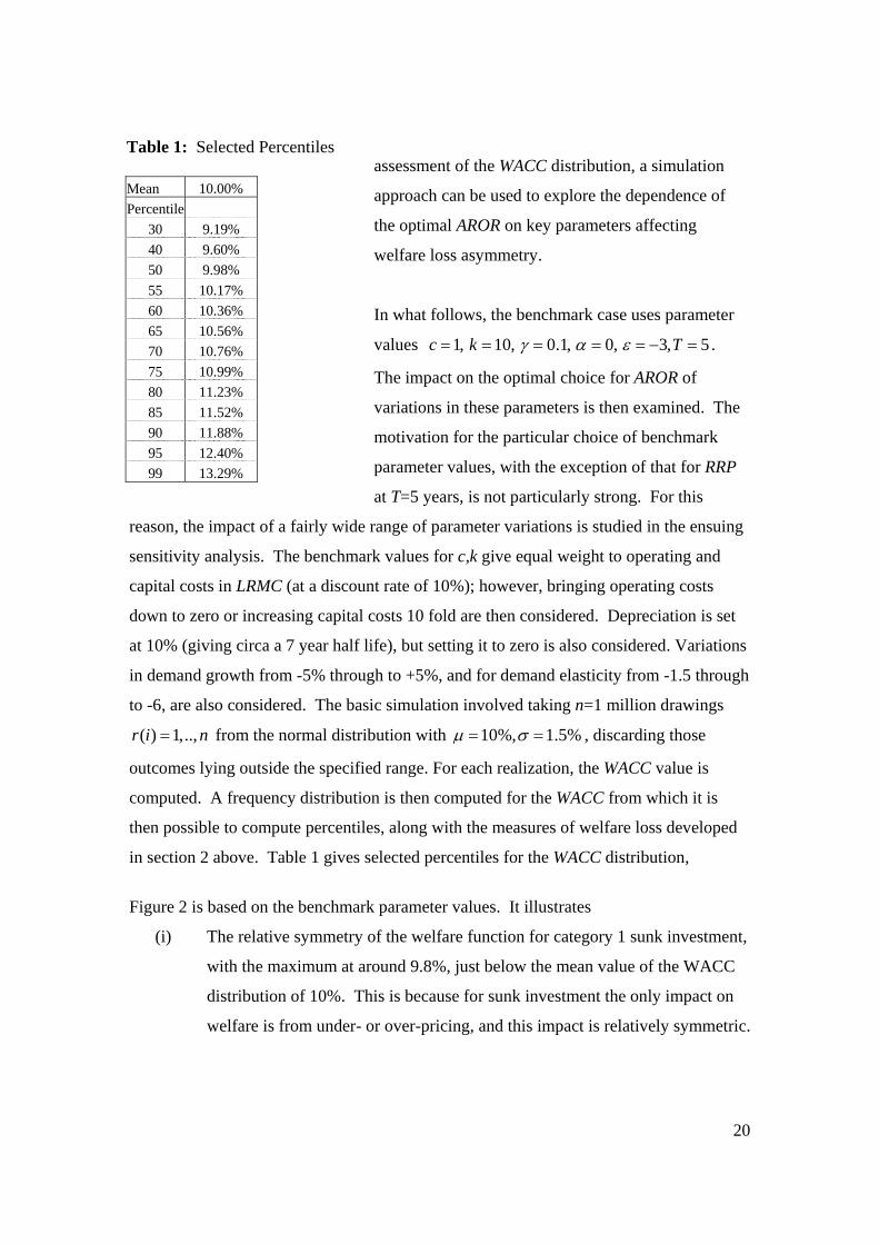
in section 2 above. Table 1 gives selected percentiles for the WACC distribution,

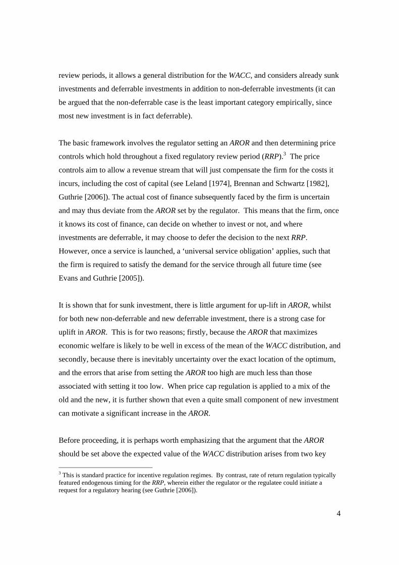
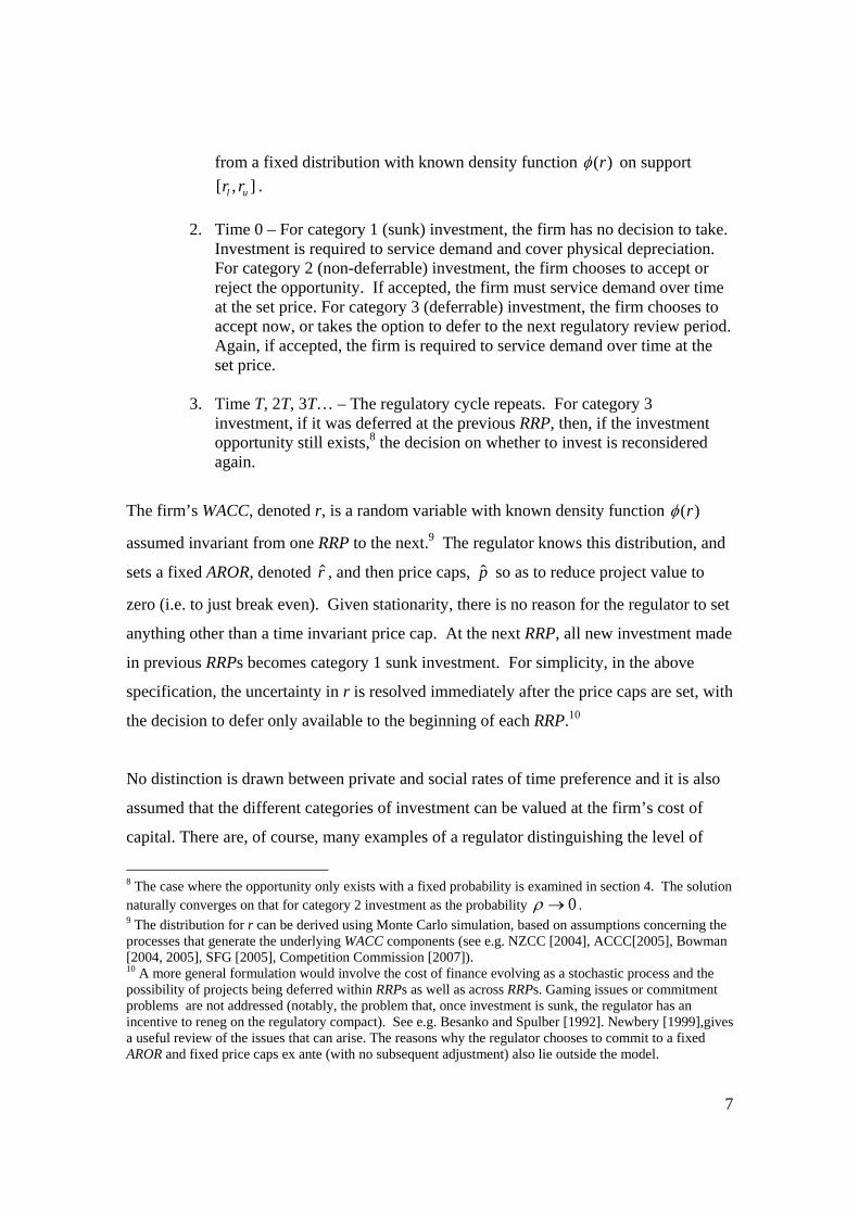
Figure 2 is based on the benchmark parameter values. It illustrates

(i) The relative symmetry of the welfare function for category 1 sunk investment,

with the maximum at around 9.8%, just below the mean value of the WACC

distribution of 10%. This is because for sunk investment the only impact on

welfare is from under- or over-pricing, and this impact is relatively symmetric.

Table 1: Selected Percentiles

Mean 10.00% Percentile

30 9.19% 40 9.60% 50 9.98% 55 10.17% 60 10.36% 65 10.56% 70 10.76% 75 10.99% 80 11.23% 85 11.52% 90 11.88% 95 12.40% 99 13.29%

21

(ii) The significant asymmetry in expected economic welfare for both category 2

(non-deferrable) and category 3 (deferrable) investments as a function of the

choice of AROR.

(a) around the mean value for WACC: there is significant increase in expected

economic welfare by increasing AROR above the mean of the WACC

distribution

(b) around the optimum choice for AROR. Although at sufficiently high

values for AROR there is some fall away in economic welfare, setting too high

an AROR is still likely to be less welfare costly than setting too low a rate.

(iii) In so far as the precise value for the optimal AROR is uncertain, it makes

sense to err on the side of setting AROR too high rather than too low.

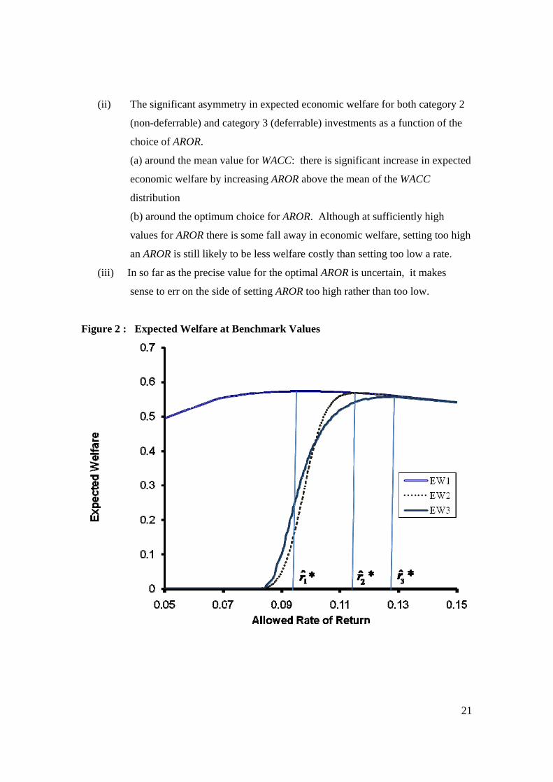
Figure 2 : Expected Welfare at Benchmark Values

22

The key feature for new investment in Figure 2, whether it is deferrable (with expected

economic welfare 3EW ) or not (with 2EW ), is that when a low value for AROR is set, the

investment rarely takes place and so economic welfare gain is small. Expected welfare

then increases rapidly as AROR is increased up to and above the WACC mean value,

eventually tailing off at high values for AROR. This is directly a result of the trade off

between the welfare benefits of incentivizing investment versus the welfare costs

associated with potential ‘overpricing’. The latter only becomes significant at higher

levels for the AROR. The other point to note is the similar structure for category 2 and 3

investments; welfare gain in both cases climbs rapidly once the AROR rises above its

mean value. The welfare gain for non-deferrable investment naturally tends to peak at a

lower AROR than that for deferrable investment, this reflecting the option value ‘gain

from waiting’.

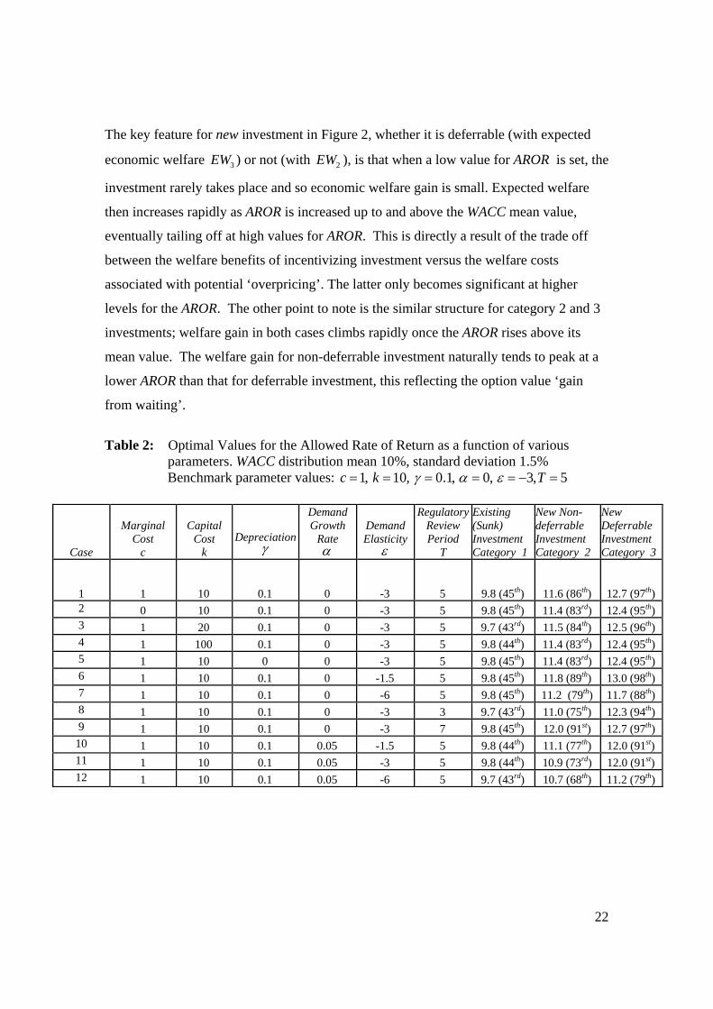
Table 2: Optimal Values for the Allowed Rate of Return as a function of various

parameters. WACC distribution mean 10%, standard deviation 1.5% Benchmark parameter values: 1, 10, 0.1, 0, 3, 5c k Tγ α ε= = = = = − =

Case

Marginal Cost

c

Capital Cost

k Depreciation

γ

Demand Growth

Rate α

Demand Elasticity

ε

Regulatory Review Period

T

Existing (Sunk) Investment Category 1

New Non-deferrable Investment Category 2

New Deferrable Investment Category 3

1 1 10 0.1 0 -3 5 9.8 (45th) 11.6 (86th) 12.7 (97th) 2 0 10 0.1 0 -3 5 9.8 (45th) 11.4 (83rd) 12.4 (95th) 3 1 20 0.1 0 -3 5 9.7 (43rd) 11.5 (84th) 12.5 (96th) 4 1 100 0.1 0 -3 5 9.8 (44th) 11.4 (83rd) 12.4 (95th) 5 1 10 0 0 -3 5 9.8 (45th) 11.4 (83rd) 12.4 (95th) 6 1 10 0.1 0 -1.5 5 9.8 (45th) 11.8 (89th) 13.0 (98th) 7 1 10 0.1 0 -6 5 9.8 (45th) 11.2 (79th) 11.7 (88th) 8 1 10 0.1 0 -3 3 9.7 (43rd) 11.0 (75th) 12.3 (94th) 9 1 10 0.1 0 -3 7 9.8 (45th) 12.0 (91st) 12.7 (97th)

10 1 10 0.1 0.05 -1.5 5 9.8 (44th) 11.1 (77th) 12.0 (91st) 11 1 10 0.1 0.05 -3 5 9.8 (44th) 10.9 (73rd) 12.0 (91st) 12 1 10 0.1 0.05 -6 5 9.7 (43rd) 10.7 (68th) 11.2 (79th)

23

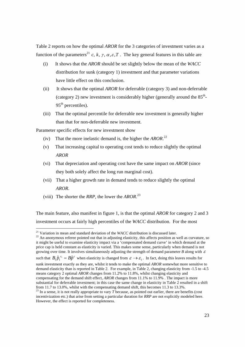
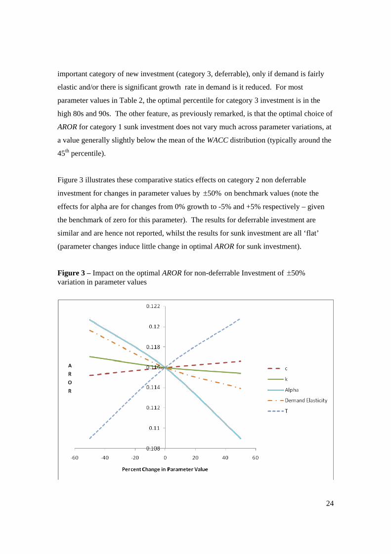
Table 2 reports on how the optimal AROR for the 3 categories of investment varies as a

function of the parameters21 , , , , ,c k Tγ α ε . The key general features in this table are

(i) It shows that the AROR should be set slightly below the mean of the WACC

distribution for sunk (category 1) investment and that parameter variations

have little effect on this conclusion.

(ii) It shows that the optimal AROR for deferrable (category 3) and non-deferrable

(category 2) new investment is considerably higher (generally around the 85th-

95th percentiles).

(iii) That the optimal percentile for deferrable new investment is generally higher

than that for non-deferrable new investment.

Parameter specific effects for new investment show

(iv) That the more inelastic demand is, the higher the AROR.22

(v) That increasing capital to operating cost tends to reduce slightly the optimal

AROR

(vi) That depreciation and operating cost have the same impact on AROR (since

they both solely affect the long run marginal cost).

(vii) That a higher growth rate in demand tends to reduce slightly the optimal

AROR.

(viii) The shorter the RRP, the lower the AROR.23

The main feature, also manifest in figure 1, is that the optimal AROR for category 2 and 3

investment occurs at fairly high percentiles of the WACC distribution. For the most 21 Variation in mean and standard deviation of the WACC distribution is discussed later. 22 An anonymous referee pointed out that in adjusting elasticity, this affects position as well as curvature, so it might be useful to examine elasticity impact via a ‘compensated demand curve’ in which demand at the price cap is held constant as elasticity is varied. This makes some sense, particularly when demand is not growing over time. It involves simultaneously adjusting the strength of demand parameter B along with ε such that 1

1 1ˆ ˆB p Bpε ε= when elasticity is changed from 1ε ε→ . In fact, doing this leaves results for sunk investment exactly as they are, whilst it tends to make the optimal AROR somewhat more sensitive to demand elasticity than is reported in Table 2. For example, in Table 2, changing elasticity from -1.5 to -4.5 means category 2 optimal AROR changes from 11.2% to 11.8%, whilst changing elasticity and compensating for the demand shift effect, AROR changes from 11.1% to 11.9% . The impact is more substantial for deferrable investment; in this case the same change in elasticity in Table 2 resulted in a shift from 11.7 to 13.0%, whilst with the compensating demand shift, this becomes 11.3 to 13.3%. 23 In a sense, it is not really appropriate to vary T because, as pointed out earlier, there are benefits (cost incentivization etc.) that arise from setting a particular duration for RRP are not explicitly modeled here. However, the effect is reported for completeness.

24

important category of new investment (category 3, deferrable), only if demand is fairly

elastic and/or there is significant growth rate in demand is it reduced. For most

parameter values in Table 2, the optimal percentile for category 3 investment is in the

high 80s and 90s. The other feature, as previously remarked, is that the optimal choice of

AROR for category 1 sunk investment does not vary much across parameter variations, at

a value generally slightly below the mean of the WACC distribution (typically around the

45th percentile).

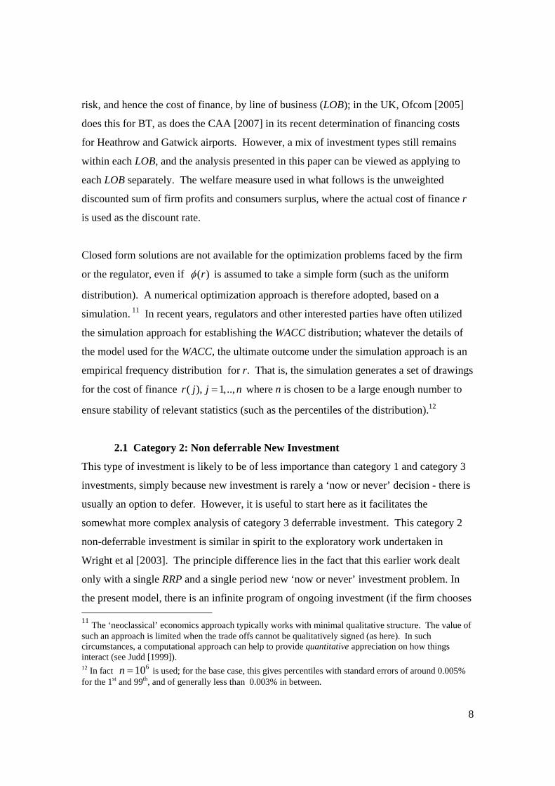
Figure 3 illustrates these comparative statics effects on category 2 non deferrable

investment for changes in parameter values by 50%± on benchmark values (note the

effects for alpha are for changes from 0% growth to -5% and +5% respectively – given

the benchmark of zero for this parameter). The results for deferrable investment are

similar and are hence not reported, whilst the results for sunk investment are all ‘flat’

(parameter changes induce little change in optimal AROR for sunk investment).

Figure 3 – Impact on the optimal AROR for non-deferrable Investment of 50%± variation in parameter values

25

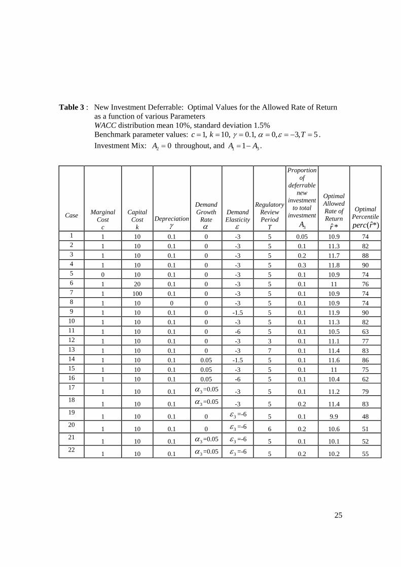
Table 3 : New Investment Deferrable: Optimal Values for the Allowed Rate of Return

as a function of various Parameters WACC distribution mean 10%, standard deviation 1.5% Benchmark parameter values: 1, 10, 0.1, 0, 3, 5c k Tγ α ε= = = = = − = . Investment Mix: 2 0A = throughout, and 1 31A A= − .

Case Marginal Cost

c

Capital Cost

k Depreciation

γ

Demand Growth

Rate α

Demand Elasticity

ε

Regulatory Review Period

T

Proportion of

deferrable new

investment to total

investment

3A

Optimal Allowed Rate of Return

ˆ*r

Optimal Percentile

ˆ( *)perc r1 1 10 0.1 0 -3 5 0.05 10.9 74 2 1 10 0.1 0 -3 5 0.1 11.3 82 3 1 10 0.1 0 -3 5 0.2 11.7 88 4 1 10 0.1 0 -3 5 0.3 11.8 90 5 0 10 0.1 0 -3 5 0.1 10.9 74 6 1 20 0.1 0 -3 5 0.1 11 76 7 1 100 0.1 0 -3 5 0.1 10.9 74 8 1 10 0 0 -3 5 0.1 10.9 74 9 1 10 0.1 0 -1.5 5 0.1 11.9 90

10 1 10 0.1 0 -3 5 0.1 11.3 82 11 1 10 0.1 0 -6 5 0.1 10.5 63 12 1 10 0.1 0 -3 3 0.1 11.1 77 13 1 10 0.1 0 -3 7 0.1 11.4 83 14 1 10 0.1 0.05 -1.5 5 0.1 11.6 86 15 1 10 0.1 0.05 -3 5 0.1 11 75 16 1 10 0.1 0.05 -6 5 0.1 10.4 62 17 1 10 0.1 3α =0.05 -3 5 0.1 11.2 79 18 1 10 0.1 3α =0.05 -3 5 0.2 11.4 83 19 1 10 0.1 0 3ε =-6 5 0.1 9.9 48 20 1 10 0.1 0 3ε =-6 6 0.2 10.6 51 21 1 10 0.1 3α =0.05 3ε =-6 5 0.1 10.1 52 22 1 10 0.1 3α =0.05 3ε =-6 5 0.2 10.2 55

26

Table 3 provides a study of how variation in underlying parameters affects the optimal

value for AROR for the case where there are is a mix of sunk and deferrable investment

(for investment categories 1 and 3 respectively, whilst the extent of non-deferrable

category 2 investment is set to zero). Give outcomes in Table 2, the results for the case

where there is a mix of sunk and non-deferrable investment (categories 1 and 2

respectively, whilst the extent of deferrable category 3 investment is set to zero) are

naturally very similar to those reported in Table 3 and so are omitted.

In table 3, rows 1-4 illustrate the impact of increasing the proportion of new deferrable

investment relative to existing, sunk, investment. In row 1, it is 5% and this is then

increased through 10, 20 to 30% new deferrable investment (setting 2 0B = and

varying 3 0.05,0.1,0.2,0.3B = , implying 1 0.95,0.9,0.8,0.7B = respectively). As a

consequence, the optimal AROR increases from the 74th percentile at 5% new investment

through to the 90th percentile when there is 30% new investment. These first four rows

illustrate a fairly general point that, even with new investment being small relative to

existing business, its impact on the optimal choice of AROR can be substantial. Even

with only 5% potentially new business investment, the 74th percentile is optimal (at

benchmark parameter values).

Row 5 shows the effect of reducing the marginal operating cost to zero. This reduces the

AROR from its benchmark value of the 82nd percentile to the 74th percentile. A similar

impact occurs if one reduces the rate of depreciation (γ ) to zero, as per row 8. This is

logical since both affect the long run margin cost equally. Rows 6 and 7 also show the

impact of increasing k relative to c and hence parallel that in row 5 (where c is reduced to

zero). These results show that greater capital to operating cost across all types of

investment) tends to reduce somewhat the percentile choice for AROR, but that the AROR

always remains above the 70th percentile. Rows 9-11 illustrate the importance of demand

elasticity; the more elastic the demand (across all types of investment), the lower the

optimal AROR will be. Elasticity appears to have this impact primarily because of its

effect on economic welfare arising from existing business. Notice in Figure 2 that 1EW ,

although peaking at around the 45th percentile, is fairly flat as a function of the choice of

27

AROR. However, as demand becomes more inelastic, the optimal AROR moves to the

left slightly, but more tellingly, the curvature of the function increases. This means that

1EW has a bigger impact in determining the maximum for the function EW in (39) (given

that there is heavy weight, 80-95%, accorded to existing sunk investment in table 3).

The impact of elasticity is even more notable if the demand associated with new

investment is more elastic than that for existing business – this is illustrated in rows 19

and 20, and also 21 and 22; here, existing business has elasticity -3 whilst new

(deferrable) business has elasticity set at -6. Even with 20% new / 80% existing business,

the AROR is not much above its mean value. Elasticity plays an even bigger role in

determining the optimal AROR here because of the impact elasticity has on the relative

magnitude of economic welfare gain. That is, reducing elasticity from -3 to -6 reduces

substantially the amount of consumer surplus that is added by new investment, and hence

reduces the welfare impact relative to that of existing business (with elasticity -3).

Finally, rows 14-16 illustrate the impact of increasing the growth rate in demand from

zero to 5% per annum (whilst also varying the elasticity of demand). The general effect

of a higher growth rate is to reduce somewhat the optimal AROR (for any given mix of

business and any given elasticity of demand etc.). Row 17 , 18, and 21, 22 then examine

the case where there is a 5% growth rate in demand and higher elasticity (-6) for new

investment compared to that for existing/sunk investment (which has 0% growth and

elasticity -3). These results are consistent with those for the unilateral variations from

benchmark values considered in Table 2 above.

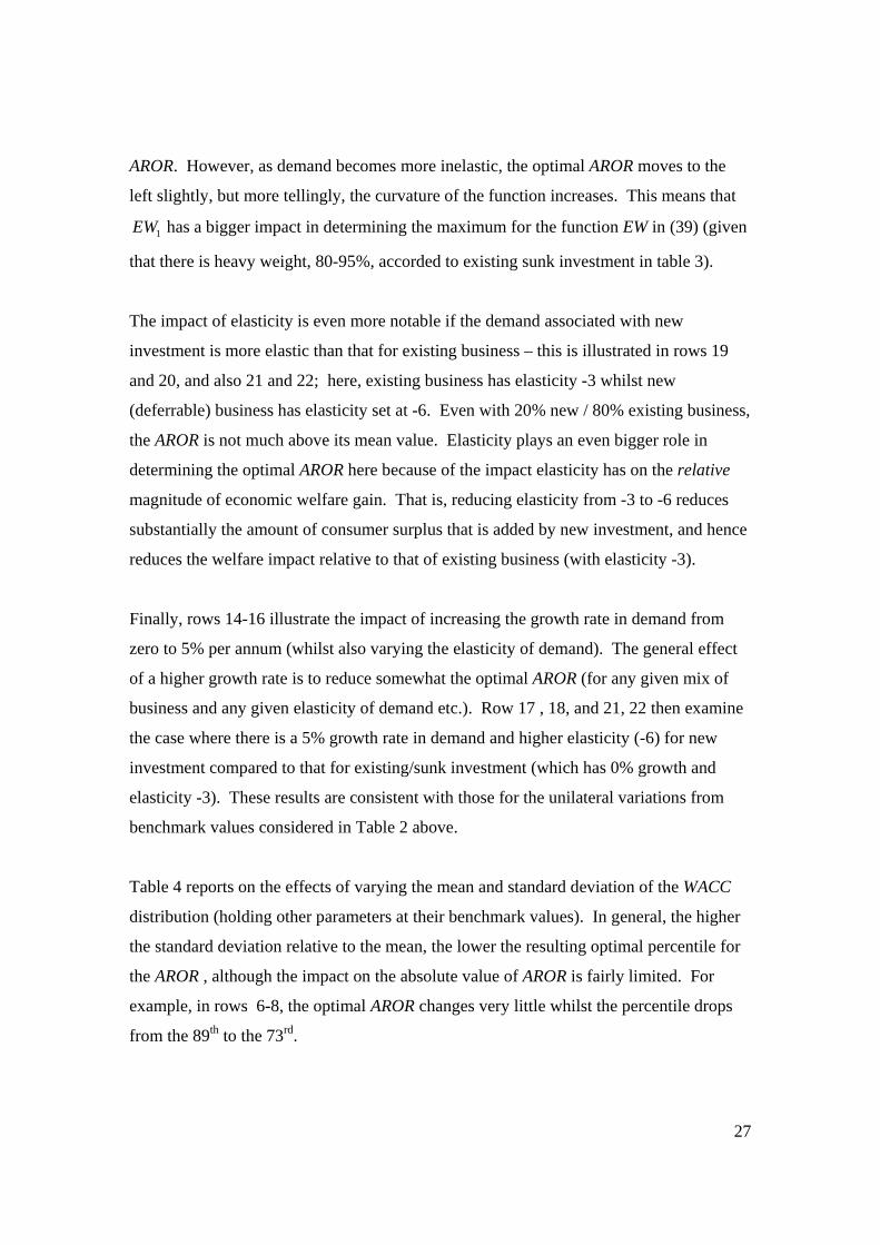
Table 4 reports on the effects of varying the mean and standard deviation of the WACC

distribution (holding other parameters at their benchmark values). In general, the higher

the standard deviation relative to the mean, the lower the resulting optimal percentile for

the AROR , although the impact on the absolute value of AROR is fairly limited. For

example, in rows 6-8, the optimal AROR changes very little whilst the percentile drops

from the 89th to the 73rd.

28

Table 4 : New Investment Deferrable: Optimal Values for the Allowed Rate of Return

as a function of WACC distribution Parameters Benchmark parameter values: 1, 10, 0.1, 0, 3, 5c k Tγ α ε= = = = = − = Weights: 1 2 30.9, 0, 0.1A A A= = = throughout.

Case

Mean μ

(%)

Standard Deviation

σ (%)

Optimal Allowed Rate of Returnˆ*r

Optimal Percentile ˆ( *)perc r

1 5 1.5 5.6 66 2 10 1.5 11.3 82 3 15 1.5 16.7 88 4 20 1.5 22 91 5 10 0.5 10.9 97 6 10 1.0 11.2 89 7 10 1.5 11.3 82 8 10 2.0 11.2 73

To summarize, the general conclusions are that

(i) if the AROR is distinguished by investment category, then it is reasonable to

set a rate close to the mean value for the WACC distribution for existing

(sunk) investments, but a much higher percentile (typically 85th – 95th) for

new business.

(ii) where the AROR is applied to a mix of investment (sunk/new deferrable or

non-deferrable), the choice of percentile depends on the characteristics of

these investments. Even a small amount of potential new investment can

induce a significant uprating in the choice of AROR and

(a) a higher percentile should be chosen the greater the likely amount of new

investment in the RRP, although

(b) a lower percentile should be chosen the more elastic demand is likely to be

– and particularly if demand associated with new investment is likely to be

more elastic than that for existing sunk investment, and

(c) to some extent a lower percentile should be chosen the more capital

intensive the investment, the more long lived the investment, and the

higher the growth rate in future demand.

29

4. Robustness of Assumptions

The model presented in section 2 is of course stylized is various ways: it assumes

constant returns to scale, a constant growth rate in demand and a constant elasticity of

demand. Inevitably, any quantitative investigation requires some specification, and hence

will be restrictive in one way or another. It can be argued that, whatever the details of

demand structures and growth in demand over time, the essential asymmetry described in

section 3 is likely to remain. For example, it is possible to construct a ‘life cycle’ model

for demand in which there is growth, maturity and decline. However, this would not be

expected to significantly alter the results obtained above. The assumption of constant

elasticity demand likewise can be modified, but would not affect the essential message.

A more important element that might attenuate the impact of AROR on economic welfare

is if the scale of investment tends to reduce costs; this is addressed in more detail in

section 4.2 below, whilst section 4.1 examines the possibility that options to defer are not

necessarily perpetual.

4.1 Options may expire

One simple modeling extension for category 3 deferrable investment is to incorporate a

probability that the option to defer investment expires in the next regulatory review

period. If ρ denotes the probability that the option to invest is still available at the next

RRP, then this modifies equation (27) to

( ) ( ) ( ) ( ) ( )c u

l c

r r rTc f cr r

EV r V r r dr e EV r r drφ ρ φ−= +∫ ∫ , (40)

and this then affects the optimal solution in equation (29), which becomes

{ }* arg max ( ) ( ) 1 ( )c u

cl c

r r rTc r fr r

r V r r dr e r drφ ρ φ−= −∫ ∫ , (41)

whilst (32) becomes

{ }*

3 *( *) ( ) ( ) 1 ( )c u

l c

r r rTc r r

EW r W r r dr e r drφ ρ φ−= −∫ ∫ . (42)

30

Clearly, if 1ρ = the solution for category 3 is the same as that reported in section 3

above. By contrast, if 0ρ = , then there is no scope for deferment and the solution is as

for category 2 investment. Thus as ρ is varied, the solution is intermediate those for

category 2 and category 3 investment reported in section 3; indeed the relationship is

fairly linear; that is, if ρ =0.5, the solution is roughly halfway between that for category 2

and category 3. For this reason a separate table is not presented for these results. The

argument in section 3 was that whether investment was deferrable or not (whether it is

category 3 or 2), there is a significant incentive to set AROR above the mean value. This

is unaffected by this modeling extension.

4.2 Investment Scale effects

One might expect that falling average costs, for example arising from economies of scale

in investment, might alter results.24 For example, in a 1-period monopoly model, setting

price equal to marginal cost gives not only zero profit but also a welfare optimum. By

contrast, in the presence of fixed costs and/or when marginal cost falls with output, a zero

profit price level lies above the welfare optimal level. Thus if average and/or marginal

costs are declining, this may give some inducement toward a lower choice for the AROR

to offset this ‘over-pricing’ impact. To explore this issue, two specifications are

considered; the first introduces a simple fixed cost term, whilst in the second, there is a

constant elasticity of scale (constant cost elasticity) for the initial level of investment. In

this case, larger initial investment drives down marginal cost. These extensions make the

price cap equation non-linear, requiring an iterative numerical solution. For this reason,

in what follows only the simpler category 2 (non-deferrable) investment case is

examined.25

(a) Scale Effect 1: Fixed costs

Here, initial investment cost is 0F kQ+ (cf. 0kQ in the original analysis). This can also

be interpreted as allowing some fall in marginal costs so long as this is ‘ infra-marginal’

24 My thanks to an anonymous referee for raising this issue. 25 There is no impact on category 1 sunk cost investment in any case, and the expected welfare function for category 3 investment is likely to continue to closely mimic that for category 2.

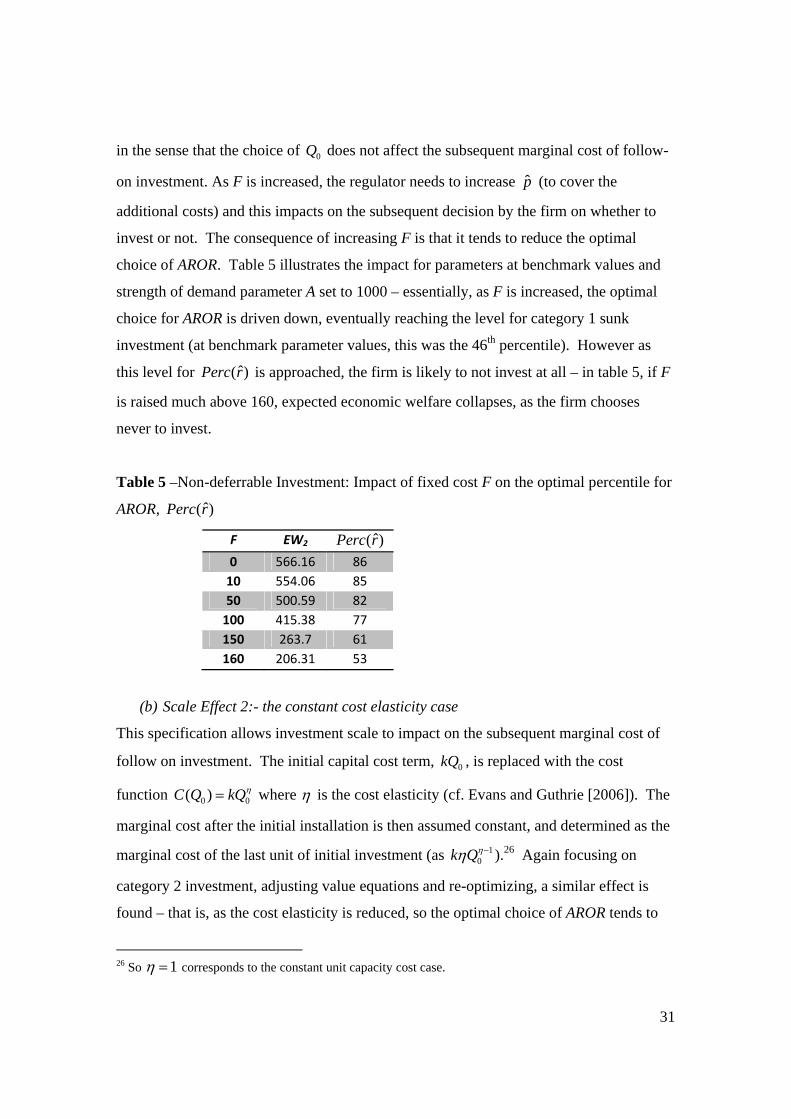
31

in the sense that the choice of 0Q does not affect the subsequent marginal cost of follow-

on investment. As F is increased, the regulator needs to increase p̂ (to cover the

additional costs) and this impacts on the subsequent decision by the firm on whether to

invest or not. The consequence of increasing F is that it tends to reduce the optimal

choice of AROR. Table 5 illustrates the impact for parameters at benchmark values and

strength of demand parameter A set to 1000 – essentially, as F is increased, the optimal

choice for AROR is driven down, eventually reaching the level for category 1 sunk

investment (at benchmark parameter values, this was the 46th percentile). However as

this level for ˆ( )Perc r  is approached, the firm is likely to not invest at all – in table 5, if F

is raised much above 160, expected economic welfare collapses, as the firm chooses

never to invest.

Table 5 –Non-deferrable Investment: Impact of fixed cost F on the optimal percentile for

AROR, ˆ( )Perc r  

F  EW2  ˆ( )Perc r0  566.16  86 10  554.06  85 50  500.59  82 100  415.38  77 150  263.7  61 160  206.31  53 

(b) Scale Effect 2:- the constant cost elasticity case

This specification allows investment scale to impact on the subsequent marginal cost of

follow on investment. The initial capital cost term, 0kQ , is replaced with the cost

function 0 0( )C Q kQη= where η is the cost elasticity (cf. Evans and Guthrie [2006]). The

marginal cost after the initial installation is then assumed constant, and determined as the

marginal cost of the last unit of initial investment (as 10k Qηη − ).26 Again focusing on

category 2 investment, adjusting value equations and re-optimizing, a similar effect is

found – that is, as the cost elasticity is reduced, so the optimal choice of AROR tends to

26 So 1η = corresponds to the constant unit capacity cost case.

32

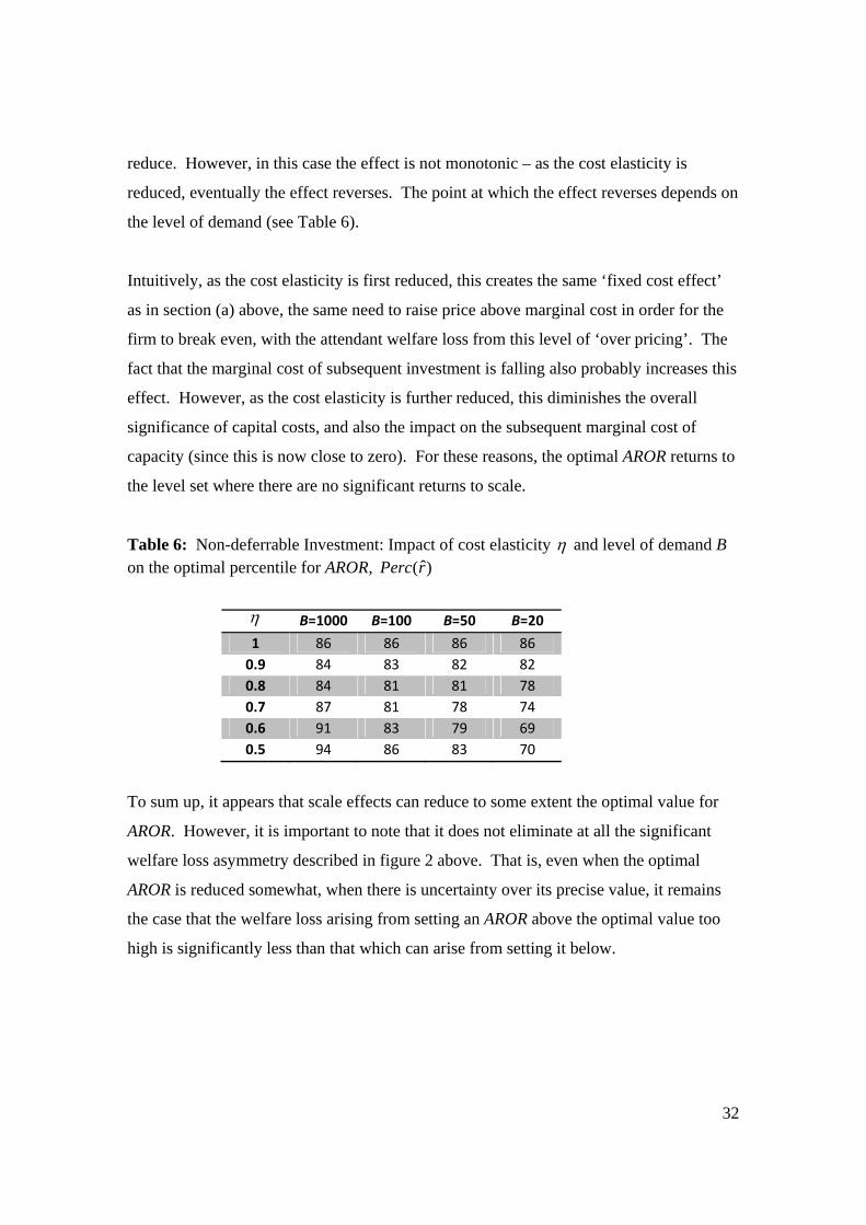
reduce. However, in this case the effect is not monotonic – as the cost elasticity is

reduced, eventually the effect reverses. The point at which the effect reverses depends on

the level of demand (see Table 6).

Intuitively, as the cost elasticity is first reduced, this creates the same ‘fixed cost effect’

as in section (a) above, the same need to raise price above marginal cost in order for the

firm to break even, with the attendant welfare loss from this level of ‘over pricing’. The

fact that the marginal cost of subsequent investment is falling also probably increases this

effect. However, as the cost elasticity is further reduced, this diminishes the overall

significance of capital costs, and also the impact on the subsequent marginal cost of

capacity (since this is now close to zero). For these reasons, the optimal AROR returns to

the level set where there are no significant returns to scale.

Table 6: Non-deferrable Investment: Impact of cost elasticity η and level of demand B on the optimal percentile for AROR, ˆ( )Perc r

η B=1000  B=100  B=50  B=20 

1  86  86  86  86 0.9  84  83  82  82 0.8  84  81  81  78 0.7  87  81  78  74 0.6  91  83  79  69 0.5  94  86  83  70 

To sum up, it appears that scale effects can reduce to some extent the optimal value for

AROR. However, it is important to note that it does not eliminate at all the significant

welfare loss asymmetry described in figure 2 above. That is, even when the optimal

AROR is reduced somewhat, when there is uncertainty over its precise value, it remains

the case that the welfare loss arising from setting an AROR above the optimal value too

high is significantly less than that which can arise from setting it below.

33

5. Conclusions

In current UK and EU regulatory practice, the estimate of what the appropriate allowed

rate of return, AROR, should be within the forthcoming regulatory review period plays an

important role in determining price controls and revenue requirements. This paper

focuses on the problem of setting a fixed allowed rate of return for the duration of a fixed

regulatory review period, given that this is but the first of an ongoing sequence of review

periods and that the allowed rate of return influences price caps and controls. When the

AROR is set ‘too low’ relative to the welfare maximizing level, this tends to result in

under investment and under pricing, whilst if it is set too high, this tends to give rise to

over-investment and over pricing.

There are two reasons for setting an AROR above the mean value of the WACC

distribution – firstly, because the value that maximizes economic welfare generally lies to

the right of the mean of the WACC distribution – and secondly, because expected

economic welfare is an asymmetric function; given the precise value of the optimal

AROR is uncertain, for each percentage point the AROR is inadvertently set above the

optimum, the welfare loss is less than that which arises from setting it an equal number of

percentage points too low. It follows that the allowed rate of return on new investments

should generally be set at a significantly higher percentile value of the WACC distribution

– that is, at percentile values in the high 80s or 90s. Where the AROR is likely to be

applied to business which involves a mix of both new and old assets, the proportions of

sunk vis a vis new investment potential within the RRP will naturally influence the extent

of uplift in the optimal choice of AROR compared to the WACC mean. However, the

asymmetry in the welfare function for new investment (vis a vis that for sunk investment)

is so strong that even if the proportions of potential new investment are quite small, this

can still induce a significant uplift in the optimal choice for the AROR compared to the

WACC mean.

34

References

Australian Consumer and Competition Commission, 2005, Assessment of Telstra’s ULLS and LSS monthly charge undertakings, Draft decision, August 2005, Appendix C. Available at www.accc.gov.au

Baron D. and Myerson R., 1982, Regulating a monopolist with unknown cost,

Econometrica, 50, 1231-1262. Besanko D. and Spulber D., 1992, Sequential equilibrium investment by regulated firms,

Rand Journal of Economics, 23(2) 153-170. Bowman R.G., 2004. “Response to WACC issues in commerce – Commissioner’s draft

report on the Gas control Enquiry.” Report prepared for PowerCo, June. Available at: www.comcom.govt.nz/RegulatoryControl/GasPipelines/ContentFiles/Documents/Submission%20-%20Powerco%20WACC%

Bowman R.G., 2005, Queensland Rail – Determination of regulated WACC, Report,

available at www.qca.org.au/www/rail/Sub_QRattach7_2005%20DAU%20Draft.pdf

Brealey R. and Franks J., 2009, Indexation, investment and utility prices, Oxford review

of economic policy, 25(3) 435-450. Brennan M.J. and Schwartz E.S., 1982, Consistent regulatory policy under uncertainty,

Bell Journal of Economics, 13(2): 506-521. BT, 2005, Ofcom’s approach to risk in the assessment of the cost of capital : BT’s

response to the Ofcom consultation document, 5/4/2005, available at http://www.btplc.com/responses.

Butler J.S. and Schachter B., 1989, The investment decision: Estimation risk and risk

adjusted discount rates, Financial Management, (4)13-22. CAA, 2008, Economic Regulation of Heathrow and Gatwick Airports 2008 -2013

– CAA Decision, available at http://www.caa.co.uk/docs/5/ergdocs /heathrowgatwickdecision_mar08.pdf

Competition Commission, 2007, BAA Ltd : A report on the economic regulation of the

London airports companies (Heathrow Airport Ltd and Gatwick Airport Ltd) available at http://www.competition-commission.org.uk/

Dixit A. and Pindyck R., 1994, Investment under Uncertainty. Princeton: Princeton

University Press.

35

Dobbs I.M., 2004, Intertemporal price cap regulation under uncertainty, Economic

Journal, 114, 421-440. Dobbs I.M., 2008, Setting the regulatory allowed rate of return using simulation and loss

functions – the case for standardizing procedures, Competition and Regulation of Network Industries, 9(3), 229-246

Evans L.T. and Guthrie G.A., 2005, Risk, price regulation and irreversible investment,

International Journal of Industrial Organization, 23, 109-128. Evans L.T. and Guthrie G.A., 2006, Incentive regulation of prices when costs are sunk,

Journal of Regulatory Economics, 29(3)239-64. First Economics, 2007. “Automatic annual adjustment of the cost of capital: A

discussion paper.” 30 March 2007. Available at www.xfi.ex.ac.uk/ conferences/costofcapital/papers/earwaker_automatic_adjustment_ of_the_cost_of_capital.pdf

Guthrie G.A., 2006, Regulating infrastructure: the impact of risk and investment,

Journal of Economic Literature, 44, 925-972. Judd K.L., 1999, Numerical methods in economics, MIT press, Cambridge, Mass. Leland H., 1974, Regulation of natural monopolies and the fair rate of return, Bell

Journal of Economics and Management Science, 5(1) 3-15. Lewis T.R.and Sappington D.E., 1988, Regulating a monopolist with unknown demand

and cost functions, Rand Journal of Economics, 19, 438-457. McDonald R. and Siegel D., 1986, ‘The value of waiting to invest’, Quarterly Journal

of Economics, vol. 101, pp. 707-728. Newbery D., 1999, Privatization, Restructuring and Regulation of Network Industries,

MIT Press, Cambridge, Mass. New Zealand Commerce Commission, 2004, Gas Control Inquiry Final Report, 29 Nov.,

2004, available at www.med.govt.nz/ers/gas/final-report/final-report.pdf. Ofcom, 2005, Ofcom’s approach to risk in the assessment of the cost of capital,

26/1/2005. Available at: http://www.ofcom.org.uk/consult/condocs/cost_capital2/

Pindyck R.S., 1988, Irreversible investment, capacity choices and the value of the firm,

American Economic Review, 78, 969-985.

36

PWC, 2006, TenneT TSO Comparison study of the WACC, Report to TenneT, May 8,

2006. Available at http://www.dte.nl/images/Comparison%20study%20of%20the%20WACC-%20Mei%202006_tcm7-87013.pdf

SFG, 2005, A framework for quantifying estimation error in regulatory WACC. Report

for Western Power in relation to the Economic Regulation Authority’s 2005 Network Access Review, 19/5/2005. Available at: http://www.wpcorp.com.au/documents/AccessArrangement/2006/Revised_AAI_Appendix_4_WACC_SFG_MAY2005.pdf

Vickers J. and Yarrow G., 1988, Privatization: An economic analysis, MIT Press,

Cambridge, Mass. Wright S., Mason R., Miles D., 2003, A study of certain aspects of the cost of capital for

regulated utilities in the U.K., 13/2/2003. The Smithers &Co. report commissioned by the UK regulators and the office of Fair Trading. Available at: www.ofcom.org.uk/static/archive/oftel/publications/pricing/2003/capt0203.pdf .

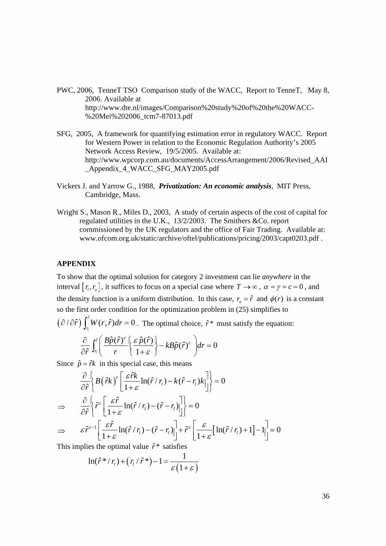
APPENDIX

To show that the optimal solution for category 2 investment can lie anywhere in the interval [ ],l ur r , it suffices to focus on a special case where T →∞ , 0cα γ= = = , and the density function is a uniform distribution. In this case, ˆar r= and ( )rφ is a constant so the first order condition for the optimization problem in (25) simplifies to

( )ˆ

ˆ ˆ/ ( , ) 0l

r

rr W r r dr∂ ∂ =∫ . The optimal choice, ˆ*r must satisfy the equation:

ˆ ˆ ˆ ˆ ˆ( ) ( ) ˆ ˆ( ) 0

ˆ 1l

r

r

Bp r p r kBp r drr r

εεε

ε⎛ ⎞∂ ⎧ ⎫− =⎨ ⎬⎜ ⎟∂ +⎩ ⎭⎝ ⎠

∫

Since ˆ ˆp rk= in this special case, this means

( ) ˆˆ ˆ ˆln( / ) ( ) 0ˆ 1 l l

rkB rk r r k r r kr

ε εε

∂ ⎧ ⎫⎡ ⎤− − =⎨ ⎬⎢ ⎥∂ +⎣ ⎦⎩ ⎭

⇒ ˆˆ ˆ ˆln( / ) ( ) 0

ˆ 1 l lrr r r r r

rε ε

ε∂ ⎧ ⎫⎡ ⎤− − =⎨ ⎬⎢ ⎥∂ +⎣ ⎦⎩ ⎭

⇒ [ ]1 ˆˆ ˆ ˆ ˆ ˆln( / ) ( ) ln( / ) 1 1 01 1l l l

rr r r r r r r rε εε εεε ε

− ⎡ ⎤ ⎡ ⎤− − + + − =⎢ ⎥ ⎢ ⎥+ +⎣ ⎦ ⎣ ⎦

This implies the optimal value ˆ*r satisfies

( ) ( )1ˆ ˆln( * / ) / * 1

1l lr r r rε ε

+ − =+

37

Now, as demand elasticity ( 1)ε < − is varied, the right hand side can vary from 0 (as ε → −∞ ) to +∞ (as 1ε → − ), so ˆ* lr r→ when demand becomes extremely elastic, whilst as it becomes more inelastic, the value for the RHS increases, and eventually, ˆ* ur r→ , the upper limit.