modeling nonnegative data with clumping at zero: …aa/articles/min_agresti_2002.pdf ·...

JIRSS (2002)

Vol. 1, Nos. 1-2, pp 7-33

Modeling Nonnegative Data with Clumping atZero: A Survey

Yongyi Min, Alan Agresti

Department of Statistics, University of Florida, Gainesville, Florida, USA32611-8545. ([email protected], [email protected])

Abstract. Applications in which data take nonnegative values buthave a substantial proportion of values at zero occur in many dis-ciplines. The modeling of such “clumped-at-zero” or “zero-inflated”data is challenging. We survey models that have been proposed. Weconsider cases in which the response for the non-zero observations iscontinuous and in which it is discrete. For the continuous and thenthe discrete case, we review models for analyzing cross-sectional data.We then summarize extensions for repeated measurement analyses(e.g., in longitudinal studies), for which the literature is still sparse.We also mention applications in which more than one clump can oc-cur and we suggest problems for future research.

1 Introduction

In some applications, the response variable can take any nonnegativevalue but has positive probability of a zero outcome. We refer toa variable as semicontinuous when it has a continuous distribution

Received: May 2002Key words and phrases: Compliance, finite mixture model, logistic regression,

Neyman type a distribution, proportional odds model, semicontinuous data, Tobitmodel, zero-inflated data.

8 Min and Agresti

except for a probability mass at 0. Semicontinuous data are commonin many areas. For example, when each observation is a record of thetotal rainfall in the previous day, many days have no rainfall. In astudy of household expenditures, some households spend nothing ona certain commodity during the period of investigation. In a studyof annual medical costs, a portion of the population has zero medicalexpense. With semicontinuous data, unlike left-censored data, thezeros represent actual response outcomes.

A related type of data are zero-inflated count data. These are datathat have a higher proportion of zeros than expected under standarddistributional assumptions such as the Poisson. Such data are alsocommon in a variety of disciplines. Examples of variables that onemight expect to be zero-inflated are observations for the past monthof the reported number of times participating in sports activities, thenumber of times one has visited a doctor, and the frequency of sexualintercourse.

One difficulty with semicontinuous data analysis is that the ex-istence of a probability mass at zero makes common response dis-tributions such as the normal or gamma inappropriate for modelingthe data. Likewise for zero-inflated count data, a generalized linearmodel based on Poisson or overdispersed count distributions usuallyencounters lack of fit due to disproportionately large frequencies ofzeros. Thus, these types of data stimulate interesting modeling prob-lems. Some statistical methodology has been developed to deal withthem. This article surveys methods that have been proposed formodeling these two types of data that have clumping at 0.

Section 2 introduces models for semicontinuous data and thensummarizes their advantages and disadvantages. Section 3 introducesmodels for zero-inflated count data. Section 4 surveys extensions ofthese two types of models to handle repeated measurement, such asin longitudinal studies. Section 5 discusses a data type that has aclump at both boundaries of a sample space, such as occurs withthe medical application of studying subjects’ compliance in takingprescribed drugs. The final section suggests possible areas for futureresearch.

2 Models for Semicontinuous Data

This section introduces some methods for modeling semicontinuousdata. The early research on modeling such data appeared mainly in

Modeling Nonnegative Data with Clumping at Zero 9

the econometrics literature. Tobin (1958) proposed a censored re-gression model to describe household expenditures on durable goods.This model is now commonly referred to as the Tobit model. The term“Tobit” arose from its similarities in derivation to the probit model,based on a normal latent variable construction described below. Sincethen, related literature contains numerous econometric applicationsas well as various generalizations of the Tobit model (e.g., Cragg 1971,Amemiya 1973, Gronau 1974, Heckman 1974, 1979). These all positan underlying normal random variable that is censored by a randommechanism.

An alternative strand of literature for semicontinuous data doesnot assume an underlying normal distribution. Duan, Manning, Mor-ris, and Newhouse (1983) proposed a two-part model to fit data on ex-penditures for medical care. Jørgensen (1987) proposed a compoundPoisson exponential dispersion model for semicontinuous data. Saei,Ward, and McGilchrist (1996) applied an ordinal response model thatrequires grouping the response outcomes into categories. The Tobitmodel and these alternative models are described in the followingsubsections.

2.1 Tobit models

For response variable Y , let yi denote the observation for subjecti, i = 1, . . . , n. The Tobit model assumes an underlying normallydistributed variable Y ∗

i such that:

yi =

{y∗i , if y∗i > 00, if y∗i ≤ 0

When y∗i ≤ 0, its value is unobserved.Including explanatory variables, the model assumes that the un-

derlying variable is generated by

y∗i = x′iβ + ui

where xi is a column vector of explanatory variable values for subjecti and {ui} are independent from a normal N(0, σ2) distribution. LetΦ(·) and φ(·) denote the cumulative distribution function (cdf) andthe probability density function (pdf) of the N(0, 1) distribution. For

10 Min and Agresti

the Tobit model, the probability of a zero response is

P (Yi = 0) = P (x′iβ + ui ≤ 0) = P (ui ≤ −x′iβ)

= Φ(−x′iβ

σ

)= 1− Φ

(x′iβ

σ

)Conditional on yi > 0, its probability density function is

f(yi;β, σ) = σ−1φ

(yi − x′iβ

σ

)Thus, the likelihood function for a sample of n independent observa-tions is

`(β, σ) =[ ∏

yi=0

{1− Φ(

x′iβ

σ

)}][ ∏

yi>0

σ−1φ

(yi − x′iβ

σ

)]

Tobin (1958) used a Newton-Raphson algorithm to find the maximumlikelihood (ML) estimates of β and σ. Amemiya (1984) presented acomprehensive survey of the Tobit model and its generalizations.1

The Tobit model assumes normality for the distribution of theerror term, with constant variance. In many applications this is un-realistic. When the model form is correct but the distribution of ui

is not normal, the ML estimators are inconsistent (Robinson 1982).Powell (1986) proposed semi-parametric estimation for the Tobit

model. He used a symmetrically trimmed least squares (STLS) esti-mator. This assumes that {ui} are symmetrically distributed aboutzero. The STLS estimator is defined as

β̂STLS = arg minβ

n∑i=1

I(x′iβ > 0)[min(yi, 2x′iβ)− x′iβ]2

where I is the indicator function. For a given β, the sum in thisexpression deletes the observations with x′iβ ≤ 0. When x′iβ > 0, thelower tail of the distribution of Yi is censored at zero; symmetricallycensoring the upper tail of the distribution (essentially by replacing yi

by min{yi, 2x′iβ}) restores the symmetry of distribution of Y ∗. Theresulting estimator β̂STLS is consistent and asymptotically normal

1James Tobin, Sterling Professor Emeritus of Economics at Yale University,won the 1981 Nobel Prize in Economics; he died on March 11, 2002.


under the symmetrical distribution assumption (Powell 1986). Aniterative procedure yields β̂STLS .

Yoo, Kim, and Lee (2001) used this method with the bootstrapto estimate the covariance matrix of β̂STLS . For M bootstrap repli-cations with estimate β̂j in replication j, their estimate is

Σ̂ =1M

M∑j=1

(β̂j − β̄STLS)(β̂j − β̄STLS)′

where β̄STLS = (1/M)∑M

j=1 β̂j . In an empirical study, Yoo et al.showed that semi-parametric estimation significantly outperforms es-timation assuming normality (i.e., the Tobit model).

2.2 Two-part models

The Tobit model allows the same underlying stochastic process todetermine whether the response is zero or positive as well as thevalue of a positive response. That is, the same parameters influencewhether the outcome is zero or positive as well as the magnitude of theoutcome, conditional on its being positive. The next two subsectionsdiscuss “two-part models” that allow the two components to havedifferent parameters.

Without assuming an underlying normal distribution, Duan et al.(1983) proposed a two-part model that uses two equations to separatethe modeling into two stages. The first stage refers to whether theresponse outcome is positive. Conditional on its being positive, thesecond stage refers to its level.

The first part is a binary model for the dichotomous event ofhaving zero or positive values, such as the logistic regression model

logit[P (Yi = 0)] = x′1iβ1

Conditional on a positive value, the second part assumes a log-normaldistribution; that is,

log(yi|yi > 0) = x′2iβ2 + εi

where εi is distributed as N(0, σ2). The likelihood function for this

12 Min and Agresti

two-part model is

`(β1,β2, σ) =[ ∏

yi=0

P (yi = 0)][ ∏

yi>0

P (yi > 0)f(yi|yi > 0)]

=[ ∏

yi=0

ex′1iβ1

1 + ex′1iβ1

][ ∏

yi>0

1

1 + ex′1iβ1

σ−1φ

(log(yi)− x′2iβ2

σ

)]Duan et al. (1983) showed that the likelihood function has a uniqueglobal maximum. ML calculations are relatively simple, because thelikelihood function factors into two terms. The first term has onlythe logit model parameters,

`1(β1) =[ ∏

yi=0

ex′1iβ1

][ n∏i=1

1

1 + ex′1iβ1

]The second term involves only the parameters of the second modelpart,

`2(β2, σ) =∏yi>0

σ−1φ


σ

)One can obtain ML estimates by separately maximizing the twoterms. Duan et al. (1983) applied this model to describe demandfor medical care. For another application, see Grytten, Holst, andLaake (1993).

2.3 Sample selection models

Heckman (1974, 1979) extended the Tobit model to a two-part model.His model has been commonly applied to model sample selectionand the related potential bias. There are many variants of sampleselection models. We use the version by van de Ven and van Praag(1981) to illustrate. For observation i, let {(u1i, u2i)} be iid from abivariate N(0,Σ) distribution, where

Σ =(

σ21 σ12

σ12 σ22

)The model assumes that

Ii = x′1iβ1 + u1i,


y∗i = x′2iβ2 + u2i,

yi = exp(y∗i ) if Ii > 0,

= 0 if Ii ≤ 0

When Ii > 0, yi > 0 is observed and y∗i = log(yi); when Ii ≤ 0, yi = 0is observed and y∗i is ‘missing’. The covariate and parameter vectors(x1i, β1) for Ii may differ from (x2i, β2) for y∗i . Two estimationmethods employed with this model are ML and a two-step proceduredue to Heckman (1979).

For ML estimation, the likelihood function of the model is givenby

`(β1,β2,Σ) =[ ∏

yi=0

P (Ii ≤ 0)][ ∏

yi>0

f(y∗i |Ii > 0)P (Ii > 0)]

=[ ∏

yi=0

P (Ii ≤ 0)][ ∏

yi>0

∫ ∞

0f(y∗i , Ii)dIi

]=

[ ∏yi=0

{1− Φ(

x′1iβ1

σ1

)}]

×[ ∏

yi>0

Φ{(

x′1iβ1

σ1+

log(yi)− x′2iβ2

σ−112 σ1σ2

2

)×(1− σ2

12σ−21 σ−2

2 )−12 }σ−1

2 φ


σ2

)]An iterative method can be used to find the ML estimates.

Heckman’s two-step procedure does not perform as well as the MLestimators. But this method is very simple and easy to implement. Itis widely used and has become the standard estimation procedure forempirical microeconometrics studies. With the two-step procedure,the subsample regression function for Y ∗

i is

E[Y ∗i |x2i, Ii > 0] = x′2iβ2 + E[u2i|u1i > −x′1iβ1] = x′2iβ2 +

σ12

σ1λi

(1)where λi = φ(zi)/Φ(zi), and zi = x′1iβ1/σ1. So, we have

log(Yi) = E[Y ∗i |x2i, Ii > 0] + εi

= x′2iβ2 +σ12

σ1λi + εi,

where Heckman (1979) showed that εi has mean 0 and varianceσ2

2[(1 − ρ2) + ρ2(1 + ziλi − λ2i )], where ρ2 = σ2

12/(σ21σ

22). One can

14 Min and Agresti

estimate the parameters β1 and σ1 by a probit model using the fullsample. Therefore, zi and hence λi can be easily estimated. Theestimated value of λi is used as a regressor in equation (1). Then onecan estimate β2 using least squares.

Duan et al. (1983, 1984) pointed out that the model has poornumerical and statistical properties. The likelihood function mayhave non-unique local maxima (Olsen 1975), and computations aremore involved than in the Duan et al. (1983) two-part model. Themodel relies on untestable assumptions in that the censored data areunobservable, so standard diagnostic methods based on the empiricalerror distribution cannot be applied. When a high correlation existsbetween λ and x2, the estimator in the sample selection model is verynonrobust. Some researchers have suggested that x1 and x2 shouldnot have variables in common, but this is not realistic in practice.

Both the Duan et al. (1983) two-part model and Heckman’s sam-ple selection model use two equations to separately model whetherthe outcome is positive and the magnitude of a positive response. Thesample selection model posits an underlying bivariate normal error.It estimates an unconditional equation that describes the level thatsubjects would have if they all had outcomes. The two-part modelestimates a conditional equation that describes only the level of out-comes for those that truly are positive. The econometrics literaturecontains discussion comparing the sample selection model and thetwo-part model. See, for instance, Duan et al. (1983, 1984), Manninget al. (1987), and Leung and Yu (1996).

2.4 Compound Poisson exponential dispersion models

Jørgensen (1987, 1997) proposed using a single distribution from theexponential dispersion family to analyze semicontinuous data. Thisdistribution is a type of compound Poisson distribution. The expo-nential dispersion family, which is used in generalized linear models,has form

f(yi; θi, φ) = c(yi, φ) exp(

θiyi − b(θi)φ

)It is characterized by its variance function v(µi), expressed in termsof the mean µi (Jørgensen 1987). For this family, θ relates to µ byµ = ∂b(θ)/∂θ. An important class of exponential dispersion modelsuses the power function, v(µ) = µp. When p = 1, this is the Poissondistribution.


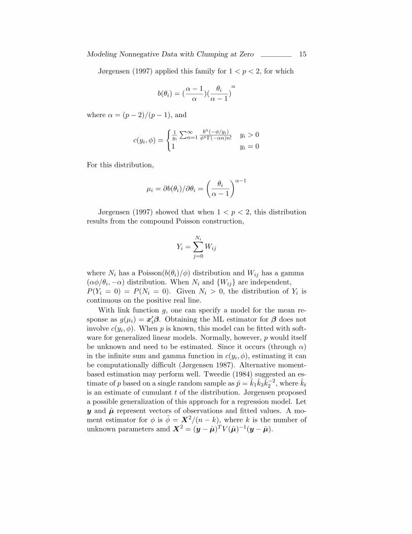
Jørgensen (1997) applied this family for 1 < p < 2, for which

b(θi) = (α− 1

α)(

θi

α− 1)α

where α = (p− 2)/(p− 1), and

c(yi, φ) =

{1yi

∑∞n=1

bn(−φ/yi)φnΓ(−αn)n! yi > 0

1 yi = 0

For this distribution,

µi = ∂b(θi)/∂θi =(

θi

α− 1

)α−1

Jørgensen (1997) showed that when 1 < p < 2, this distributionresults from the compound Poisson construction,

Yi =Ni∑j=0

Wij

where Ni has a Poisson(b(θi)/φ) distribution and Wij has a gamma(αφ/θi,−α) distribution. When Ni and {Wij} are independent,P (Yi = 0) = P (Ni = 0). Given Ni > 0, the distribution of Yi iscontinuous on the positive real line.

With link function g, one can specify a model for the mean re-sponse as g(µi) = x′iβ. Obtaining the ML estimator for β does notinvolve c(yi, φ). When p is known, this model can be fitted with soft-ware for generalized linear models. Normally, however, p would itselfbe unknown and need to be estimated. Since it occurs (through α)in the infinite sum and gamma function in c(yi, φ), estimating it canbe computationally difficult (Jørgensen 1987). Alternative moment-based estimation may perform well. Tweedie (1984) suggested an es-timate of p based on a single random sample as p̂ = k̂1k̂3k̂

−22 , where k̂t

is an estimate of cumulant t of the distribution. Jørgensen proposeda possible generalization of this approach for a regression model. Lety and µ̂ represent vectors of observations and fitted values. A mo-ment estimator for φ is φ̂ = X2/(n − k), where k is the number ofunknown parameters amd X2 = (y − µ̂)T V (µ̂)−1(y − µ̂).

16 Min and Agresti

2.5 Ordinal threshold models

Saei, Ward, and McGilchrist (1996) suggested grouping the possibleoutcome values into k ordered categories and applying an ordinal re-sponse model. Let Yg be the grouped response variable. The thresh-old model for an ordinal response posits an unobservable variable Z,such that one observes Yg = j (i.e., in category j) if Z is betweenθj−1 and θj . Suppose that Z has a cumulative distribution functionG(z − η), where η is related to explanatory variables by

η = x′β

Then,

P (Yg ≤ j) = P (Z ≤ θj) = G(θj − x′β)

The threshold model then follows, by which

G−1[P (Yg ≤ j;x)] = θj − x′β, j = 1, 2, . . . , k − 1

That is, the inverse of the cdf serves as the link function.In application with semicontinuous data and a clump at 0, one

would take the first category to be the 0 outcome, and then one wouldselect cutpoints on the positive outcome scale to define the other k−1categories. Assuming that G is logistic leads to a logit model for thecumulative probabilities, called a cumulative logit model. Assumingthat G is normal leads to a cumulative probit model (McCullagh1980). A score test is available to check the assumption that covariateeffects are the same for each cutpoint (Peterson and Harrell 1990).Chang and Pocock (2000) applied the cumulative logit model formodeling the amount of personal care for the elderly.

This model has the simplicity of a single model to handle theclump at 0 and the positive outcomes. Elements of β summarizeeffects overall, rather than conditional on the response being posi-tive. For instance, to compare different groups that are levels of theexplanatory variables, one can use β̂ directly, whereas for two-partmodels one needs to average results from the two components of themodel to make an unconditional comparison (e.g., to estimate E(Y )for the groups). Two obvious concerns with this model are that theway the positive scale is collapsed into categories is arbitrary, and bygrouping the data one loses some information.


2.6 Advantages and disadvantages of existingapproaches

The Tobit model was the first to deal with semicontinuous data. Thesample selection model extends the Tobit model to allow differentcoefficients to affect the two components. Both models assume anunderlying normal random variable that is censored by a randommechanism. These models are sometimes suitable for modeling alimited or censored response variable. When zeros represent actualoutcome values instead of censored or missing values, the underly-ing normal assumption becomes dubious. By contrast, the Duan etal. (1983) two-part model has several appealing properties, includinga well-behaved likelihood function and more appropriate interpreta-tions than the Tobit and Heckman models if the zeros are true values.

The compound Poisson exponential dispersion model makes itpossible to analyze data with a single model that includes both as-pects described in the two-part model. In this sense, it is relativelysimple. Given the power p in the variance function, this model iseasy to fit, but otherwise the model seems problematic. It does notseem to have received attention in practice other than in Jørgensen’swork. Ordinal response models also can model the zero and non-zerovalues in one model, and they are simple to fit. A drawback is thatthey model grouped data instead of the original data.

Of these models, it seems to us that the Duan et al. (1983) two-part model is a reasonable choice for many applications. Comparedwith other models we’ve discussed, this model addresses the datain their original form, is simple to fit, and is relatively simple tointerpret.

3 Models for Zero-Inflated Count Data

Count responses with a relatively large clump at zero can occur inmany situations (e.g., Cameron and Trivedi 1998, pp. 10-15). Havinga large number of observations at zero is not by itself sufficient to ruleout a particular discrete distribution. However, often the remainingcounts show considerable variability, which is inconsistent with thePoisson distribution (for which the mean determines both the vari-ance and the probability at 0). This may be caused by overdispersiondue to unobserved heterogeneity. Then, a distribution that allows thePoisson mean to vary at fixed values of predictors may be appropri-

18 Min and Agresti

ate. Examples are the negative binomial regression model (whichcan be derived with a gamma mixture of Poisson means) and thegeneralized linear mixed model that adds a normal random effect toa model for the log of the Poisson mean. See, for instance, Cameronand Trivedi (1998) and Chapter 13 of Agresti (2002) for discussionof such approaches.

Sometimes such simple models for overdispersion are themselvesinadequate. For instance, the data might be bimodal, with a clumpat zero and a separate hump around some considerably higher value.This might happen for variables for which a certain fraction of thepopulation necessarily has a zero outcome, and the remaining frac-tion follows some distribution having positive probability of a zerooutcome. This happens for variables referring to the number of timesone takes part in a certain activity, when some subjects never do soand others may occasionally not do so. Examples are the numberof papers one published in the previous year (for a sample of profes-sors), and the number of times one exercised in a gym in the previousmonth. For such zero-clumped data, standard discrete distributionsare suspect. The above representation of two types of subjects leadsnaturally to a mixture model, some examples of which are presentedin this section on the modeling of zero-inflated count data.

3.1 Zero-inflated discrete distributions

Lambert (1992) introduced zero-inflated Poisson (ZIP) regression mod-els to account for overdispersion in the form of excess zero counts forthe Poisson distribution. Since her article, zero-inflated discrete mod-els have been developed and applied in the econometrics and statisticsliterature.

Lambert’s model treats the data as a mixture of zeros and out-comes of Poisson variates. For subject i, she assumed that

Yi ∼

{0 with probability pi

Poisson(λi) with probability 1− pi

The resulting distribution has

P (Yi = 0) = pi + (1− pi)e−λi ,

P (Yi = j) = (1− pi)e−λiλj

i

j!, j = 1, 2, . . .


With explanatory variables, the parameters are themselves modeledby

logit(pi) = x′1iβ1 and log(λi) = x′2iβ2

The log likelihood function is

L(β1,β2) =∑yi=0

log[ex′1iβ1 + exp(−ex

′2iβ2)]

+∑yi>0

(yix′2iβ2 − ex

′2iβ2)

−n∑

i=1

log(1 + ex′1iβ1)−

∑yi>0

log(yi!)

A latent class construction that yields this model posits an unob-served binary variable Zi. When Zi = 1, yi = 0, and when Zi = 0,Yi is Poisson(λi). Lambert (1992) suggested using the EM algorithmfor ML estimation of the parameters, treating zi as a missing value.

Hall (2000) adapted Lambert’s method to an upper-bounded countsetting to yield a zero-inflated binomial model. With upper boundfor Yi of ni, he took

Yi ∼

{0 with probability pi

binomial(ni, πi) with probability 1− pi

He modeled pi with logit(pi) = x′1iβ1 and modeled πi with logit(πi)= x′2iβ2, using the EM algorithm to obtain ML estimates.

In practice, overdispersion is common with count data, even con-ditional on a positive count or for a component of a latent class model.The equality of mean and variance assumed by the ZIP model, con-ditional on Zi = 0, is often not realistic. Zero-inflated negative bino-mial models would likely often be more appropriate than ZIP models.Grogger and Carson (1991) used zero-truncated Poisson models to fitdata simulated from zero-truncated negative binomial distributions.They observed biases of estimated parameters up to 30 percent. Sim-ilar arguments extend to zero-inflated models. With an inappropri-ate Poisson assumption, standard error estimates can be biased verydramatically. Ridout, Hinde and Demetrio (2001) provided a scoretest for testing zero-inflated Poisson models against the zero-inflatednegative binomial alternative. For an application of the zero-inflatednegative binomial model, see Shankar, Milton, and Mannering (1997).

With more than a single unusually high probability, extensions ofzero-inflated count models may be needed. For instance, in studying

20 Min and Agresti

Swedish female fertility, Melkersson and Rooth (2000) inspected thenumber of births for a sample of women. They found more 0 and 2outcomes than expected in a standard count data model. They useda multinomial logit model to estimate the extra probabilities of zeroand two children.

3.2 Hurdle models

The hurdle model is a two-part model for count data proposed byMullahy (1986). One part of the model is a binary model, suchas logistic or probit regression, for whether the response outcome iszero or positive. If the outcome is positive, the “hurdle is crossed.”Conditioning on a positive outcome, to analyze its level the secondpart uses a truncated model that modifies an ordinary distributionby conditioning on a positive outcome. This might be a truncatedPoisson or truncated negative binomial. Applications of such modelshave been given by Pohlmeier and Ulrich (1995), Arulampalam andBooth (1997), and Gurmu and Trivedi (1996).

Suppose we use a logistic regression for the binary process and atruncated Poisson model for the positive outcome; that is,

logit[P (Yi = 0)] = x′1iβ1 and log(λi) = x′2iβ2

The log likelihood then has two components:

L1(β) =∑yi=0

[log P1(yi = 0;β1,x1i)]

+∑yi>0

[log(1− P1(yi = 0;β1,x1i))]

=∑yi=0

x′1iβ1 −n∑

i=1

log(1 + ex′1iβ1)

is the log-likelihood function for the binary process, and

L2(β2) =∑yi>0

[yix′2iβ2 − ex

′2iβ2 − log(1− e−ex

′2iβ2 )]−

∑yi>0

log(yi!)

is the log-likelihood function for the truncated model. The joint log-likelihood function is

L(β1,β2) = L1(β1) + L2(β2)


One can maximize this by separately maximizing L1 and L2.In some applications, the data may have a long right tail reflecting

some extremely large positive counts. Gurmu (1997) proposed a semi-parametric hurdle model for a highly skewed distribution of counts.It is based on a Laguerre series expansion for the unknown densityof the unobserved heterogeneity.

3.3 Finite mixture models

Another approach for zero-inflated count data uses a finite mixturemodel. It assumes that the response comes from a mixture of severallatent distributions. With q latent groups, the mixture density is

f(yi;θ) =q∑

j=1

πjfj(yi; θj), y = 0, 1, 2, . . .

where πj is the true proportion in group j, fj(yi; θj) is the massfunction (e.g., Poisson or negative binomial) for group j, and {πj}and {θj} are unknown parameters. The zero-inflated count modelsof Sec. 3.1 are special cases of the finite mixture model in whichone of the mixture mass functions is degenerate at zero. The moregeneral mixture model allows for additional population heterogeneitybut avoids the sharp dichotomy between the population of zeros andnon-zero counts.

One approach to fitting a finite mixture model relates it to latentclass analysis (Aitkin and Rubin 1985). Let dij denote an indicatorto represent whether yi comes from latent group j, with

∑j dij = 1.

Assume that {(yi, di1, . . . , diq), i = 1, . . . , n} are independent, suchthat {dij , j = 1, . . . , q} have the multinomial distribution

q∏j=1

πdij

j

and conditional on their values, yi has probability mass functionq∑

j=1

dijf(yi; θj) =q∏

j=1

f(yi; θj)dij , yi = 0, 1, 2, . . .

Then, the likelihood function is

`(θ,π) =n∏

i=1

[ q∑j=1

πdij

j f(yi; θj)dij

]

22 Min and Agresti

Treating {dij} as missing data, one can use the EM algorithm to fitthe model.

Deb and Trivedi (1997) used a finite mixture model to study thedemand for medical care by the elderly. They found that a two-point mixture negative binomial model fits better than the standardnegative binomial model and its hurdle extension. Wedel et al. (1993)applied this method to analyze the effects of direct marketing on bookselling. Gerdtham and Trivedi (2001) used it in studying the equityissue in Swedish health care.

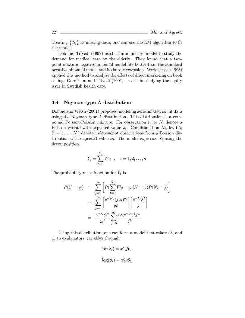
3.4 Neyman type A distribution

Dobbie and Welsh (2001) proposed modeling zero-inflated count datausing the Neyman type A distribution. This distribution is a com-pound Poisson-Poisson mixture. For observation i, let Ni denote aPoisson variate with expected value λi. Conditional on Ni, let Wit

(t = 1, . . . , Ni) denote independent observations from a Poisson dis-tribution with expected value φi. The model expresses Yi using thedecomposition,

Yi =Ni∑t=0

Wit , i = 1, 2, . . . , n

The probability mass function for Yi is

P (Yi = yi) =∞∑

j=0

[P (

Ni∑t=0

Wit = yi|Ni = j)P (Ni = j)]

=∞∑

j=0

[e−jφi(jφi)yi

yi!

][e−λiλj

i

j!

]

=e−λiφyi

i

yi!

∞∑j=0

(λie−φi)jjyi

j!

Using this distribution, one can form a model that relates λi andφi to explanatory variables through

log(λi) = x′1iβ1,

log(φi) = x′2iβ2


Since E(Yi) = λiφi,

log[E(Yi)] = log(λi) + log(φi) = x′1iβ1 + x′2iβ2

Dobbie and Welsh used a four-step procedure with the Newton-Raph-son algorithm to estimate parameters, iterating between estimatingβ1 for a given β2 and estimating β2 for a given β1. The infinite sumsin the density function make model-fitting complicated. They appliedit to model the abundance of Leadeater’s Possum in mountain ashforests of southeastern Australia. Here, λi denotes the mean numberof possum clusters per site, and φi denotes the average number ofpossums per cluster.

3.5 Advantages and disadvantages of existingapproaches

The zero-inflated model and the hurdle model are similar. The zero-inflated models are more natural when it is reasonable to think ofthe population as a mixture, with one set of subjects that necessarilyhas a 0 response. However, they are more complex to fit, as themodel components must be fitted simultaneously. By contrast, onecan separately fit the two components in the hurdle model. Thehurdle model is also suitable for modeling data with fewer zeros thanwould be expected under standard distributional assumptions.

The finite mixture model is semi-parametric. If the observationscan realistically be viewed as being drawn from different populations,this approach is attractive. A potential disadvantage with this modelis that it may overestimate the number of components when there isa lack of model fit. The Neyman type A model makes it possible tofit the data using a single distribution. However, it is not a memberof the exponential family, so the mathematical and inferential advan-tages associated with this family are not available, and model fittingis complicated by the infinite sum in the mass function.

4 Modeling Repeated Measurement of Zero-Clumped Data

Compared with the substantial literature on cross-sectional observa-tions of data with clumping at zero, few papers have discussed the

24 Min and Agresti

modeling of clustered, correlated observations, such as occur withlongitudinal data. This section surveys this literature.

4.1 Repeated measurement of semicontinuous data

Cowles, Carlin, and Connett (1996) and Hajivassiliou (1994) ex-tended the Tobit model and the sample selection model to longitu-dinal data. Both models assume an underlying normal distribution,which is dubious in most applications, especially when zeros repre-sent actual responses instead of censored or missing values. We donot discuss their approaches here. Olsen and Schafer (2001) extendedthe two-part model of Duan et al. (1983) to longitudinal data. Wedescribe their model next.

Let yij be the semicontinuous response for subject (or cluster)i (i = 1, . . . , n) at occasion j (j = 1, . . . , ti). The first part of themodel is a logistic random effects model for the dichotomous eventof having zero or positive values. Suppose that

yij

{= 0 with probability pij

6= 0 with probability 1− pij

Let {ci} be random effects to account for within-subject correlation.Conditional on ci, we assume that

logit(pij) = x′1ijβ1 + z′1ijci

where x1ij and z1ij are covariate vectors pertaining to the fixed effectsβ and random effects ci. In practice, the simple random interceptform of model is often adequate, in which ci = ci is univariate andz1ij = 1.

In the second part of the model, let

Vij =

{yij , if yij > 0unspecified, if yij = 0

When Vij is positive, conditional on a random effect di the modelassumes that Vij follows a log-normal distribution. Thus, the modelfor the positive outcomes is

log(Vij) = x′2ijβ2 + z′2ijdi + εij


where the residuals {εij} are assumed to be independent from N(0, σ2).Again, often the simple random intercept form of model is often ad-equate, in which di = di is univariate and z2ij = 1.

When the response is observed at repeated times, a high level of apositive response at one time may affect the probability of a positiveoutcome at another time. So, one can tie the two parts of the modeltogether by taking the random effects from the two parts as jointlynormal and correlated,

bi =(

ci

di

)∼ N (0, Σ)

where

Σ =(

Σcc Σcd

Σdc Σdd

)To fit the model, one first obtains a marginal likelihood by integrat-ing out the random effects. However, these integrals are analyticallyintractable, so the marginal likelihood does not have a closed-formexpression. Numerical or stochastic approximation of the integralsis needed, as in the fitting of generalized linear mixed models (e.g.,Agresti 2002, Chapter 12). With univariate random intercepts, nu-merical approximation using Gauss-Hermite quadrature, which ap-proximates the integral by a finite sum, should be adequate. Thenone can maximize the approximated likelihood using standard opti-mization methods such as Newton–Raphson.

Olsen and Schafer (2001) studied many fitting methods. Theycompared Markov chain Monte Carlo (MCMC), the EM algorithm,penalized quasi-likelihood (PQL), Gauss-Hermite quadrature, andLaplace approximations. Simulations by Raudenbush et al. (2000)showed that a high-order Laplace approximation can be as accurateas Gauss-Hermite quadrature yet is much faster than the other meth-ods. Olsen and Schafer noted that it took MCMC and EM algorithmsmore than one day to obtain accurate estimates for their example,while the sixth-order Laplace method needed less than one minute.

Saei et al. (1996) extended the ordinal threshold model to ana-lyze clustered semicontinuous data. Again, this requires breaking thecontinuous scale into categories. Let yij,g be the grouped responsefor observation j on subject i. Let G be the cumulative distribu-tion function for an underlying unobservable variable. For outcomecategory k, the model assumes

P (Yij,g ≤ k) = G(θk − ηij)

26 Min and Agresti

whereηij = x′ijβ + z′ijbi

for a vector bi ∼ N(0,Σ) of random effects that account for within-subject correlation. They took G to be the standard normal cdf,yielding a cumulative probit model, and they used penalized quasi-likelihood (PQL) to fit the model.

4.2 Repeated measurement of zero-inflated data

As with semicontinuous data, there is little literature on modelingclustered zero-inflated count data. Hall (2000) extended the zero-inflated Poisson and zero-inflated binomial models to handle longitu-dinal data, adding random effects to account for the within-subjectdependence.

Hall assumed that Yij = 0 with probability pij andYij ∼ Poisson(λij) with probability 1 − pij . The parameters pij andλij are modeled by

logit(pij) = x′1ijβ1,

log(λij) = x′2ijβ2 + bi

where bi ∼ N(0, σ2) is a random effect. The Poisson(λij) distributionapplies conditional on bi; unconditionally, there is overdispersion rel-ative to the Poisson when σ > 0. The log-likelihood function for thelongitudinal zero-inflated Poisson model is

L(β1,β2, σ) =n∑

i=1

[log

∫ +∞

−∞[

ti∏j=1

P (Yij = yij |bi)]φ(bi)dbi

]Hall employed the EM algorithm with Gauss-Hermite quadrature tofit the model. In a corresponding longitudinal zero-inflated binomialmodel, Hall assumed that Yij is binomial(ni, πij) with probability 1−pij (conditional on a random effect bi), where logit(πij) = x′2ijβ2 +bi.

Note that Hall’s model does not have a random effect for the partof the model determining the zero inflation. By contrast, Yau and Lee(2001) proposed adding a pair of uncorrelated normal random effects(bi, ci) for the two components of a hurdle model. They used a logisticmodel for the probability pij of a positive outcome. Conditional onpositive outcome, they applied a loglinear model for the mean λij ina truncated (conditionally) Poisson distribution. That is,

logit(pij) = x′1ijβ1 + bi,


log(λij) = x′2ijβ2 + ci

With uncorrelated random effects, the two components of the hurdlemodel can be fitted separately. Yau and Lee used a penalized quasi-likelihood approach for this.

5 An Application with Two Boundary Clumps

The form of data discussed in this article usually has only a singleclump, occurring at zero, or a clump at zero and a mound aroundsome larger value. Some applications, however, have data with twoclumps, one at zero and one at the maximum possible response value.

An application in which such data commonly occur is in the studyof patient compliance. Compliance is usually defined as the extentto which a subject’s behavior (in terms of taking medications, fol-lowing diets, or executing lifestyle changes) coincides with medicalor health advice (Haynes, Taylor, and Sackett 1979). The responsedistribution usually has a proportion of subjects with 0% compliance,a proportion of subjects with 100% compliance, and other subjectshaving compliances spread between 0% and 100%. An appropriatemodel permits two clumps with positive probability at the extremesand treats the remaining scale as continuous.

Thus far, little attention has been paid to specialized models forcompliance data. One possibility uses the logit to transform the re-sponse values between zero and one to the real line, as is often donewith compositional data (Aitchison and Shen 1980) and continuousproportion data (Bartlett 1937). However, this transformation can-not handle 0% or 100% compliance. Another possibility is to use aquasi-likelihood approach with variance function v(µ) = [µ(1 − µ)]2

(Wedderburn 1974), which corresponds to constant asymptotic vari-ance for the logit of compliance. Another possibility is to use the Saeiet al. (1996) approach with ordered categories for the outcomes, inwhich the extreme outcomes refer to the clumped outcomes. We arecurrently conducting research on models for this form of data.

6 Future Research

For cross-sectional nonnegative data with clumping at zero, we havesurveyed a considerable amount of research. However, methods for

28 Min and Agresti

longitudinal data are less developed and could use more work. Forinstance, it may be of interest to extend the exponential dispersionmodel with V (µ) = µp (1 < p < 2) to longitudinal data analysis. Sofar this method has essentially been ignored even for cross-sectionalanalysis.

Or, one could develop further the ordinal threshold model forlongitudinal data analysis. Saei et al. (1996) proposed a cumulativeprobit model to fit clustered semicontinuous data, and they used a pe-nalized quasi-likelihood (PQL) approach to estimate the parameters.However, Breslow and Lin (1995) showed that the PQL estimatesare biased and inconsistent for binomial responses when the randomeffects have large variance and the binomial denominator is small.We suspect that using the PQL approach to fit the cumulative probitmodel will have similar problems. The use of different distributionfunctions and more accurate estimation algorithms is open for futureresearch. This type of model is also suitable for zero-inflated countdata analysis. For ordinal threshold models, study is also neededabout how close the parameters fitted by the grouped data tend tobe to the ones fitted by ungrouped data.

In analyzing longitudinal count data with a zero-inflated Poissonmodel, Hall (2000) added a random intercept only to one componentof the model. Yau and Lee (2001) added a pair of random effects toboth components of a hurdle model. However, they assumed uncor-related random effects and used PQL for model fitting. When theresponse is observed at several occasions, a high positive outcome atone time may affect the probability of a positive outcome at anothertime. These two processes are likely correlated and influenced bycovariates in different ways. It makes sense to allow correlated ran-dom effects in the model, which then requires a more complex fittingprocess, preferably using ML.

For semicontinuous data analysis, most of the methods we men-tioned assume that the positive continuous responses have a log-normal distribution. This need not be realistic, especially in ap-plications in which some especially large observations create a righttail that is too long for a log-normal distribution. For instance, in asurvey of medical care expenses, the right tail may be poorly modeledby the log normal. Semi-parametric methods may be appropriate forsuch highly skewed data. Finally, the modeling of compliance dataand other types of data with more than one clump remains a fertilearea for future research.


Acknowledgments

This research was partially supported by grants from NIH and NSF.The authors thank Dr. Alan Hutson for suggesting compliance dataas a form of data possibly handled by some zero-clumped models.

References

Agresti, A. (2002), Categorical Data Analysis. 2nd Edition, Wiley.

Aitchison, J. and Shen, S. M. (1980), Logistic-normal distributions:Some properties and uses. Biometrika, 67, 261–272.

Aitkin, M. and Rubin, D. B. (1985), Estimation and hypothesistesting in finite mixture models. Journal of the Royal StatisticalSociety, Series B, Methodological, 47, 67–75.

Amemiya, T. (1973), Regression analysis when the dependent vari-able is truncated normal. Econometrica, 41, 997–1016.

Amemiya, T. (1984), Tobit models: A survey. Journal of Econo-metrics, 24, 3–61.

Arulampalam, W. and Booth, A.L. (1997), Who gets over the train-ing hurdle? A study of the training experiences of young menand women in Britain. Journal of Population Economics, 10,197–217.

Bartlett, M. S. (1937), Some examples of statistical methods of re-search in agriculture and applied biology. Supplement to theJournal of the Royal Statistical Society, 4, 137–183.

Breslow, N. E. and Lin, X. (1995), Bias correction in generalisedlinear mixed models with a single component of dispersion.Biometrika, 82, 81–91.

Cameron, A. C. and Trivedi, P. K. (1998), Regression Analysis ofCount Data. Cambridge University Press.

Chang, B. -H., Pocock, S. (2000), Analyzing data with clumping atzero – an example demonstration. Journal of Clinical Epidemi-ology, 53, 1036–1043.

30 Min and Agresti

Cowles, M. K. and Carlin, B. P. and Connett, J. E. (1996), BayesianTobit modeling of longitudinal ordinal clinical trial compliancedata with nonignorable missingness. Journal of the AmericanStatistical Association, 91, 86–98.

Cragg, J. G. (1971), Some statistical models for limited dependentvariables with application to the demand for durable goods.Econometrica, 39, 829–844.

Deb, P. and Trivedi, P. K. (1997), Demand for medical care bythe elderly: A finite mixture approach. Journal of AppliedEconometrics, 12, 313–336.

Dobbie, M. and Welsh, AH. (2001), Models for zero-inflated countdata using the Neyman type a distribution. Statistical Mod-elling, 1, 65–80.

Duan, N., Manning, W. G. Jr., Morris, C. N., and Newhouse, J.P. (1983), A comparison of alternative models for the demandfor medical care (Corr: V2 P413). Journal of Business andEconomic Statistics, 1, 115–126.

Duan, N., Manning, W. G. Jr., Morris, C. N., and Newhouse, J. P.(1984), Choosing between the sample-selection model and themulti-part model. Journal of Business and Economic Statistics,2, 283–289.

Gerdtham, U. G. and Trivedi, P. K. (2001), Equity in swedish healthcare reconsidered: New results based on the finite mixturemodel. Health Economics, 10, 565–572.

Green, P. J. (1984), Iteratively reweighted least squares for maxi-mum likelihood estimation, and some robust and resistant al-ternatives (with discussion). Journal of the Royal StatisticalSociety, Series B, Methodological, 46, 149–192.

Grogger, J. T. and Carson, R. T. (1991), Models for truncatedcounts. Journal of Applied Econometrics, 6, 225–238.

Gronau, R. (1974), Wage comparisons – a selectivity bias. Journalof Political Economy, 82, 1119–1144.

Grytten, J., Holst, D., and Laake, P. (1993), Accessibility of dentalservices according to family income in A non-insured popula-tion. Social Science & Medicine, 37, 1501–1508.


Gurmu, S. and Trivedi, P. K. (1996), Excess zeros in count mod-els for recreational trips. Journal of Business and EconomicStatistics, 14, 469–477.

Gurmu, S. (1997), Semi-parametric estimation of hurdle regressionmodels with an application to medicaid utilization. Journal ofApplied Econometrics, 12, 225–242.

Hajivassiliou, V. A. (1994), A simulation estimation analysis of theexternal debt crises of developing countries. Journal of AppliedEconometrics, 9, 109–131.

Hall, D. B. (2000), Zero-inflated poisson and binomial regressionwith random effects: a case study. Biometrics, 56, 1030–1039.

Haynes, R. B., Taylor, D. W., and Sackett, D. L. (1979), Compliancein Health Care. Johns Hopkins University Press.

Heckman, J. (1974), Shadow prices, market wages, and labor supply.Econometrica,42, 679–694.

Heckman, J. (1979), Sample selection bias as a specification error.Econometrica, 47, 153–161.

Jørgensen, B. (1987), Exponential dispersion models. Journal of theRoyal Statistical Society, Series B, Methodological, 49, 127–145.

Jørgensen, B. (1997), The theory of dispersion models. Chapman &Hall, 6.

Lambert, D. (1992), Zero-inflated poisson regression, with an appli-cation to defects in manufacturing. Technometrics, 34, 1–14.

Leung, S. F. and Yu, S. (1996), On the choice between sample selec-tion and two-part models. Journal of Econometrics, 72, 197–229.

Manning, W. G. and Duan, N. and Rogers, W. H. (1987), Montecarlo evidence on the choice between sample selection and two-part models. Journal of Econometrics, 35, 59–82.

McCullagh, P. (1980), Regression models for ordinal data. Journalof the Royal Statistical Society, Series B, Methodological, 42,109–142.

32 Min and Agresti

Melkersson, M. and Rooth, D. (2000), Modeling female fertility us-ing inflated count data models. Journal of Population Eco-nomics, 13, 189–203.

Mullahy, J. (1986), Specification and testing of some modified countdata models. Journal of Econometrics, 33, 341–365.

Olsen, MK. and Schafer, JL. (2001), A two-part random-effectsmodel for semicontinuous longitudinal data. Journal of theAmerican Statistical Association, 96, 730–745.

Olsen, R. (1975), The analysis of two-variable models when one ofthe variables is dichotomous. Yale Unversity, Economics Dept.unpublished manuscript.

Peterson, B. and Harrell, F. E. (1990), Partial proportional oddsmodels for ordinal response variables. Applied Statistics, 39,205–217.

Pohlmeier, W. and Ulrich, V. (1995), An econometric model of thetwo-part decision making process in the demand of health care.Journal of Human Resources, 30, 339–361.

Powell, J. L. (1986), Symmetrically trimmed least squares estima-tion for tobit models. Econometrica, 54, 1435–1460.

Raudenbush, S. W., Yang, M. -L. and Yosef, M. (2000), Maximumlikelihood for generalized linear models with nested random ef-fects via high-order laplace approximation. Journal of Compu-tational and Graphical Statistics, 9, 141–157.

Ridout, M. and Hinde, J. and Demetrio, CGB. (2001), A score testfor testing a zero-inflated poisson regression model against zero-inflated negative binomial alternatives. Biometrics, 57, 219–223.

Robinson, P. M. (1982), On the asymptotic properties of estimatorsof models containing limited dependent variables. Economet-rica, 50, 27–42.

Saei, A., Ward, J. and McGilchrist, C. A. (1996), Threshold modelsin a methadone programme evaluation. Statistics in Medicine,15, 2253–2260.


Shankar, V., Milton, J. and Mannering, F. (1997), Modeling acci-dent frequencies as zero-altered probability processes: an em-pirical inquiry. Accident Analysis and Prevention, 29, 829–837.

Tobin, J. (1958), Estimation of relationships for limited dependentvariables. Econometrica, 26, 24–36.

Tweedie, M. C. K. (1984), An index which distinguishes betweensome important exponential families. Statistics Applicationsand New Directions, Proceedings of the Indian Statistical Insti-tute Golden Jubilee International Conference, Indian StatisticalInstitute (Calcutta), 579–604.

Van de Ven, W. and Van Praag, B. (1981), The demand for de-ductibles in private health insurance: a probit model with sam-ple selection. Journal of Econometrics, 17, 229–252.

Wedderburn, R. W. M. (1974), Quasi-likelihood functions, general-ized linear models, and the Gauss-Newton method. Biometrika,61, 439–447.

Wedel, M., DeSarbo, W. S., Bult, J. R., and Ramaswamy, V. (1993),A latent class poisson regression model for heterogeneous countdata. Journal of Applied Econometrics, 8, 397–411.

Yau, K. K. and Lee, A. H. (2001), Zero-inflated poisson regressionwith random effects to evaluate an occupational injury preven-tion programme. Statistics in Medicine, 20, 2907–2920.

Yoo, S. H., Kim, T. Y., and Lee, J. K. (2001), modeling zero responsedata from willingness to pay surveys – A semi-parametric esti-mation. Economics Letters, 71, 191–196.

Zorn, C. J. W. (1998), An analytic and empirical examination ofzero-inflated and hurdle poisson specifications. Sociological Meth-ods & Research, 26, 368–400.

modeling nonnegative data with clumping at zero: …aa/articles/min_agresti_2002.pdf ·...

Documents