http://www.diva-portal.org

Postprint

This is the accepted version of a paper published in International Journal of Electrical Power & EnergySystems. This paper has been peer-reviewed but does not include the final publisher proof-correctionsor journal pagination.

Citation for the original published paper (version of record):

Yang, W., Yang, J., Guo, W., Norrlund, P. (2016)

Response time for primary frequency control of hydroelectric generating unit.

International Journal of Electrical Power & Energy Systems, 74: 16-24

http://dx.doi.org/10.1016/j.ijepes.2015.07.003

Access to the published version may require subscription.

N.B. When citing this work, cite the original published paper.

Permanent link to this version:http://urn.kb.se/resolve?urn=urn:nbn:se:uu:diva-259529

Response Time for Primary Frequency Control of Hydroelectric Generating Unit 1

Weijia Yanga,b,*1, Jiandong Yanga, Wencheng Guoa, Per Norrlundb,c 2

a The State Key Laboratory of Water Resources and Hydropower Engineering Science, Wuhan 3

University, Wuhan, 430072, China 4

b Department of Engineering Sciences, Uppsala University, Uppsala, SE-751 21, Sweden 5

c Vattenfall R&D, Älvkarleby, SE-814 26, Sweden 6

Abstract. For evaluating the power quality in primary frequency control for hydroelectric 7

generating units, the power response time is an indicator which is of main concern to the power 8

grid. The aim of this paper is to build a suitable model for conducting reliable simulation and to 9

investigate the general rules for controlling the power response time. Two huge hydropower 10

plants with surge tank from China and Sweden are applied in the simulation of a step test of 11

primary frequency control, and the result is validated with data from full scale measurements. 12

From the analytical aspect, this paper deduces a time domain solution for guide vane opening 13

response and a response time formula, of which the main variables are governor parameters. Then 14

the factors which cause the time difference, between the power response time and the analytical 15

response time of opening, are investigated from aspects of both regulation and water way system. 16

It is demonstrated that the formula can help to predict the power response and supply a flexible 17

guidance of parameter tuning, especially for a hydropower plant without surge tank. 18

19

Key words: Primary frequency control; Response time; Hydropower; Governor parameter; 20

Numerical simulation. 21

1* Corresponding author. Telephone number: +46 722793911 fax: +46 18 4715810 E-mail address: Weijia.Yang@Angstrom.uu.se (Weijia Yang)

22

1 Introduction 23

In order to suppress the power grid frequency fluctuation, generating units change their power 24

output automatically according to the change of grid frequency, to make the active power 25

balanced again. This is the primary frequency control. Hydroelectric generating units are suited to 26

undertake the power response in primary frequency control, because of great rapidity and 27

amplitude of the power regulation. Nowadays the power quality of hydroelectric generating units 28

in primary frequency control becomes more and more important, due to the more complex 29

structure of the grid and greater proportion of the renewable intermittent sources. The key of 30

evaluating the regulation quality is the power response time (more details are in Section 2). 31

Therefore, these problems are highly concerned by industry: How do the regulation and water 32

way system affect the response time? How should governor parameter be set to control the power 33

response time? 34

35

To the best of the authors’ knowledge, no specific research on response time of primary 36

frequency control exists currently. Simulation and dynamic process analysis of primary frequency 37

control for hydroelectric generating units are treated in e.g. reference [1-4]. The stability problem 38

is discussed in reference [5-7]. Different new controllers or control techniques are studied to 39

improve the dynamic performance of hydropower plant (HPP) in the load frequency control [8-40

11]. A series of important research activities regarding frequency control were conducted: a 41

complex simulation was performed to investigate an incident of oscillatory behavior in power 42

output of a HPP [12]; A specification was proposed for the transient and steady-state responses of 43

a HPP operating in frequency-control mode. The specification gives a generic definition of how 44

the electrical power should respond to step, ramp and random changes in frequency [13]. Based 45

on control theory, power response process was deduced by applying the transfer functions and 46

inverse Laplace transform [13]. The idea is a good inspiration to this paper. 47

48

Generally speaking, both regulation and water way system directly affects the power response 49

time. Hence the previous research can be extended in two directions, as described below. Aiming 50

at the regulation system, there are several research activities on governor parameter optimization 51

through the preliminary deduction, sensitivity analysis [3] or optimization algorithms [14, 15]. 52

However, the research on the relationship between power response and governor parameter 53

choice is in urgent need. Besides, the former simulations mostly adopt some built-in algorithm 54

directly, for example one of the differential equation solvers in MATLAB, and do not discuss the 55

accuracy and applicability of the solving methods of governor equations. On the other hand, the 56

water way subsystem in most models is relatively simple, which influences the accuracy of power 57

response. Moreover, the influence of surge and water hammer is seldom discussed deeply. 58

59

The aim of this paper is to build a suitable model for conducting reliable simulations and to 60

display general rules to obtain a desired power response. Section 2 introduces the test and 61

relevant specifications of primary frequency control, and illustrates the definition and importance 62

of the response time and delay time. Applying Visual C++ 2008, Section 3 presents the modified 63

model of turbine governor with primary frequency control function under guide vane opening 64

feedback control mode. The implementation is based on the existing mathematical model 65

described in [16], which takes into account nonlinear factors such as turbine characteristics and 66

pipeline elasticity. In Section 4, two huge HPPs with surge tank from China and Sweden are 67

applied in the simulation of a step test process of primary frequency control, and the result is 68

validated with data from full scale measurements. Section 5 conducts theoretical analysis and 69

simulation to study the response time and the influencing factors. The main results are in Section 70

5. Section 6 draws the conclusion. 71

2 Test method and specifications of primary frequency control 72

Strictly speaking, the test of primary frequency control needs to be conducted in every HPP to 73

confirm a set of parameters to meet the requirement of specifications. There are two normal test 74

methods [3]. (1) The first test method is to cut the governor input signal of frequency 75

measurement so that the regulation system is under open-loop control. Then, a required frequency 76

step signal is given, and the active power is recorded to check whether the regulation system meet 77

the specifications of the power grid operator. This test method can yield an accurate result 78

without being influenced by the change of grid frequency, but it nevertheless brings the hidden 79

danger [3] which might be caused by signal errors and wrong parameter settings. (2) The second 80

approach is to keep the units connected to the power system and step change the given frequency 81

of the governor. This method would affect the power system frequency, and the result might has 82

tiny errors because the generator frequency follows the system frequency which is not exactly the 83

rated value (50 Hz). Therefore an accurate simulation is indeed important. 84

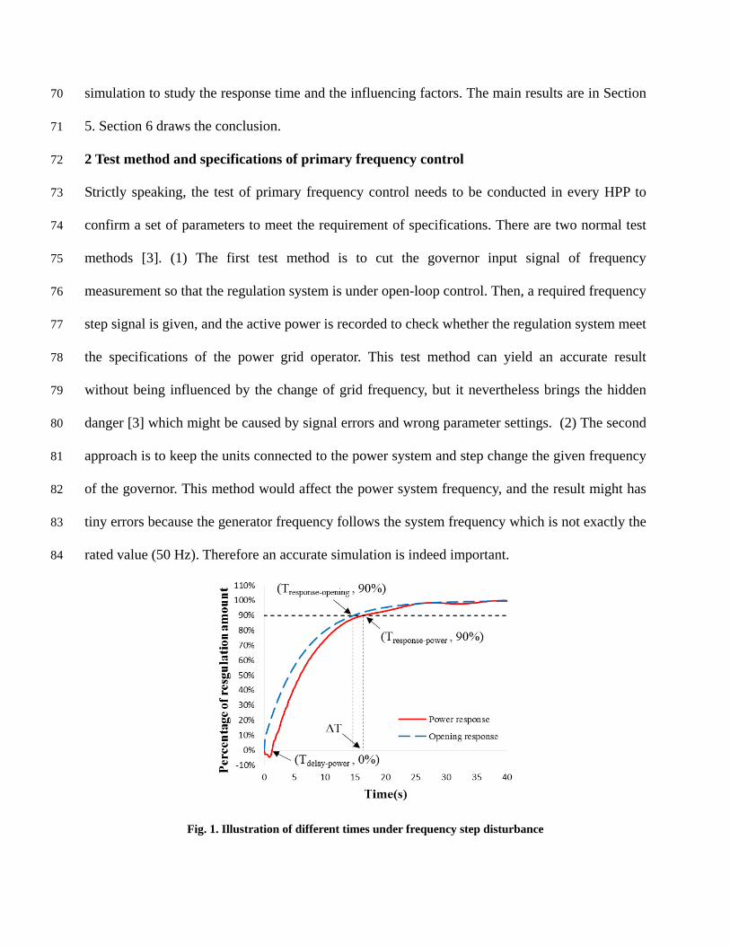
Fig. 1. Illustration of different times under frequency step disturbance

85

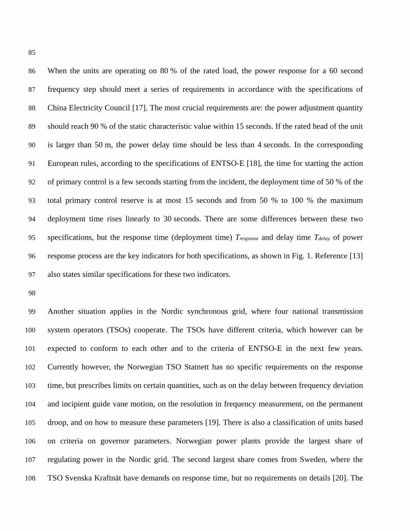
When the units are operating on 80 % of the rated load, the power response for a 60 second 86

frequency step should meet a series of requirements in accordance with the specifications of 87

China Electricity Council [17]. The most crucial requirements are: the power adjustment quantity 88

should reach 90 % of the static characteristic value within 15 seconds. If the rated head of the unit 89

is larger than 50 m, the power delay time should be less than 4 seconds. In the corresponding 90

European rules, according to the specifications of ENTSO-E [18], the time for starting the action 91

of primary control is a few seconds starting from the incident, the deployment time of 50 % of the 92

total primary control reserve is at most 15 seconds and from 50 % to 100 % the maximum 93

deployment time rises linearly to 30 seconds. There are some differences between these two 94

specifications, but the response time (deployment time) Tresponse and delay time Tdelay of power 95

response process are the key indicators for both specifications, as shown in Fig. 1. Reference [13] 96

also states similar specifications for these two indicators. 97

98

Another situation applies in the Nordic synchronous grid, where four national transmission 99

system operators (TSOs) cooperate. The TSOs have different criteria, which however can be 100

expected to conform to each other and to the criteria of ENTSO-E in the next few years. 101

Currently however, the Norwegian TSO Statnett has no specific requirements on the response 102

time, but prescribes limits on certain quantities, such as on the delay between frequency deviation 103

and incipient guide vane motion, on the resolution in frequency measurement, on the permanent 104

droop, and on how to measure these parameters [19]. There is also a classification of units based 105

on criteria on governor parameters. Norwegian power plants provide the largest share of 106

regulating power in the Nordic grid. The second largest share comes from Sweden, where the 107

TSO Svenska Kraftnät have demands on response time, but no requirements on details [20]. The 108

requirements depend on the magnitude of the frequency deviation, and if it exceeds 0.1 Hz, 50 % 109

should be delivered within 5 s, and 100 % within 30 s. 110

111

3 Modeling 112

The modeling and improvement described in this section are based on the software TOPSYS [16], 113

which is developed for analyzing transient processes of HPPs. The basic equations of water 114

conduit and hydraulic turbine behavior in TOPSYS have the following characteristics: (1) Elastic 115

water hammer is adopted in the draw water tunnel, considering the elasticity of water and pipe 116

wall. (2) Characteristic of the penstock is taken into account. (3) Characteristic curve of the 117

turbine is introduced. These are mostly simplified or ignored in the related research. However, the 118

current TOPSYS version cannot simulate primary frequency control. Therefore the governor 119

model is established here to extend the TOPSYS with this supplement implemented in VC++. 120

121

3.1 Turbine governor 122

Generally, there are two control modes for the primary frequency control of hydroelectric 123

generating unit (hereafter referred to as opening control and power control), according to 124

different feedback objects in closed-loop control: guide vane opening and power. The power 125

control mode is also called “power droop”. Since the opening control is the most common one, 126

the model of governor for primary frequency control under opening control is built and described 127

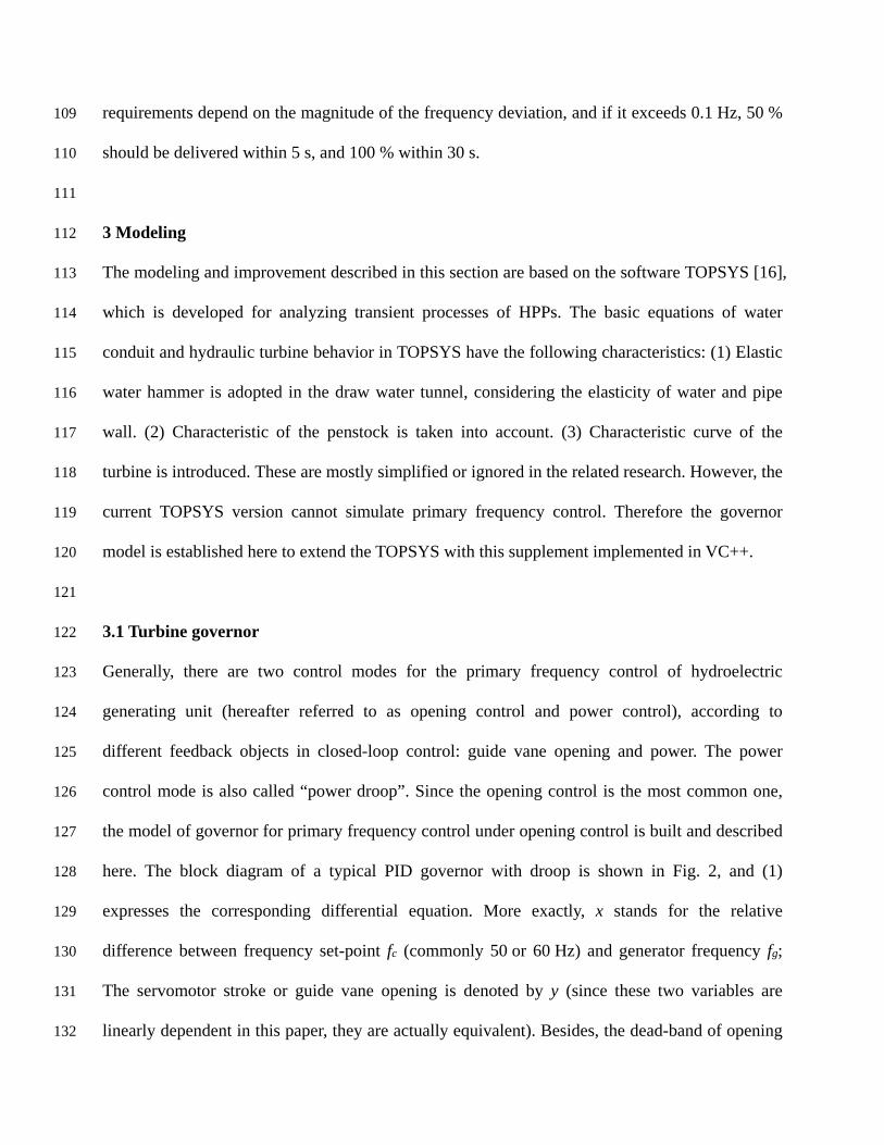
here. The block diagram of a typical PID governor with droop is shown in Fig. 2, and (1) 128

expresses the corresponding differential equation. More exactly, x stands for the relative 129

difference between frequency set-point fc (commonly 50 or 60 Hz) and generator frequency fg; 130

The servomotor stroke or guide vane opening is denoted by y (since these two variables are 131

linearly dependent in this paper, they are actually equivalent). Besides, the dead-band of opening 132

and frequency are contained in the model. Their effect can be reflected in simulations, but they 133

are omitted in (1) because of their nonlinear nature. The remaining symbols are Kp, Ki and Kd that 134

are standard PID-parameters, bP denoting droop, and Ty representing lag in main servo motor. 135

136

3 2

3 2

2

2

( ) (1 ) ( )p d y y p p y d p p p p i y p i c

d p i

d y d y dyb K T T b K T K K b K b K T b K y ydt dt dt

d x dxK K K xdt dt

+ + + + + + + −

= + +

(1)

137

Fig. 2. Block diagram of governor under opening control 138

3.2 Simplified generator 139

In the currently relevant simulations, the generator frequency is given directly in the form of a 140

step function, and it does not need to be obtained by a generator equation. 141

142

3.3 Engineering case 143

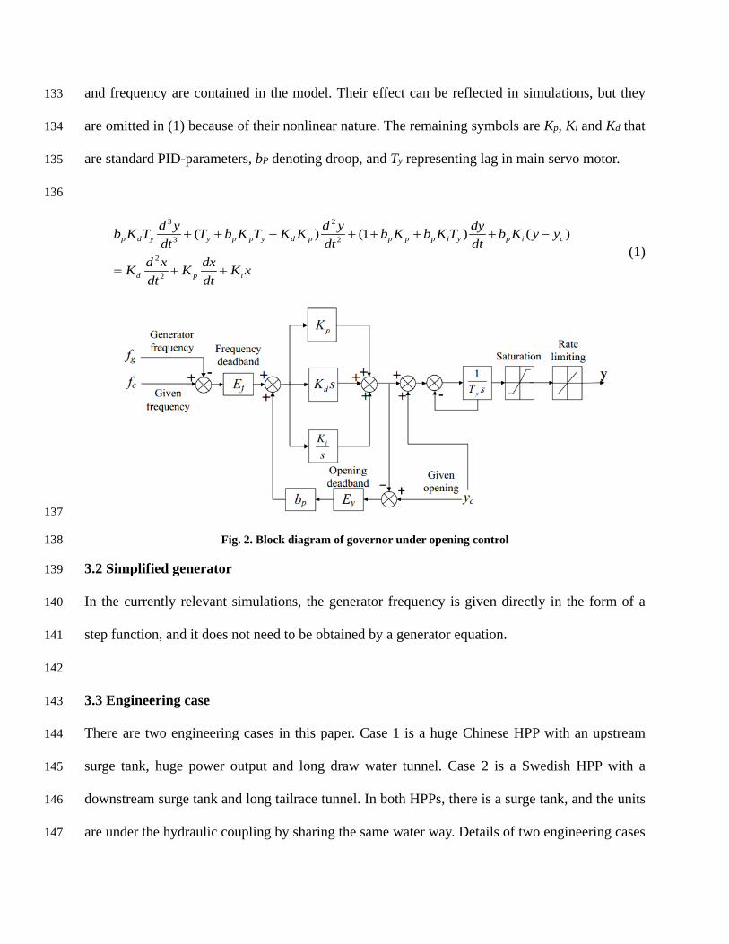
There are two engineering cases in this paper. Case 1 is a huge Chinese HPP with an upstream 144

surge tank, huge power output and long draw water tunnel. Case 2 is a Swedish HPP with a 145

downstream surge tank and long tailrace tunnel. In both HPPs, there is a surge tank, and the units 146

are under the hydraulic coupling by sharing the same water way. Details of two engineering cases 147

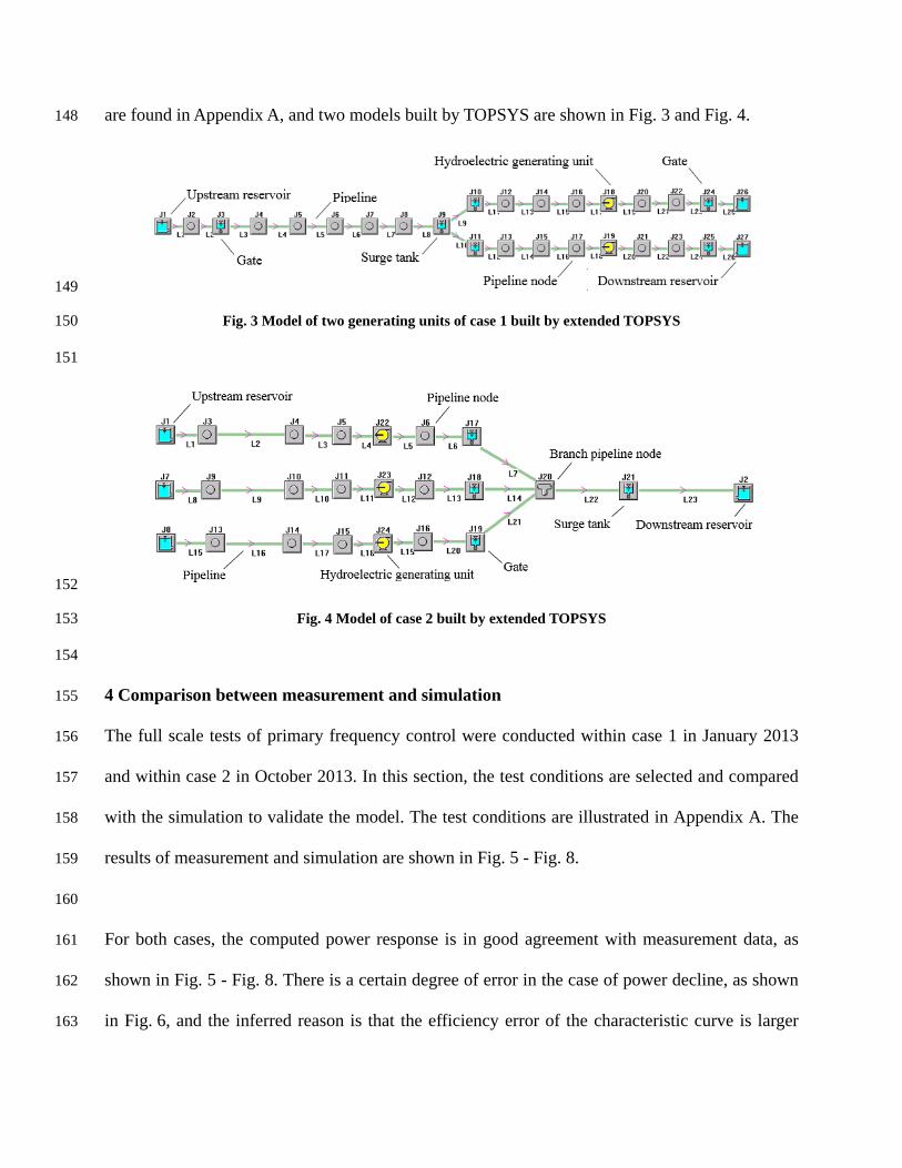
are found in Appendix A, and two models built by TOPSYS are shown in Fig. 3 and Fig. 4. 148

149

Fig. 3 Model of two generating units of case 1 built by extended TOPSYS 150

151

152

Fig. 4 Model of case 2 built by extended TOPSYS 153

154

4 Comparison between measurement and simulation 155

The full scale tests of primary frequency control were conducted within case 1 in January 2013 156

and within case 2 in October 2013. In this section, the test conditions are selected and compared 157

with the simulation to validate the model. The test conditions are illustrated in Appendix A. The 158

results of measurement and simulation are shown in Fig. 5 - Fig. 8. 159

160

For both cases, the computed power response is in good agreement with measurement data, as 161

shown in Fig. 5 - Fig. 8. There is a certain degree of error in the case of power decline, as shown 162

in Fig. 6, and the inferred reason is that the efficiency error of the characteristic curve is larger 163

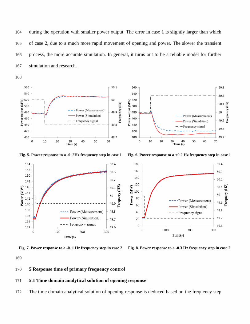
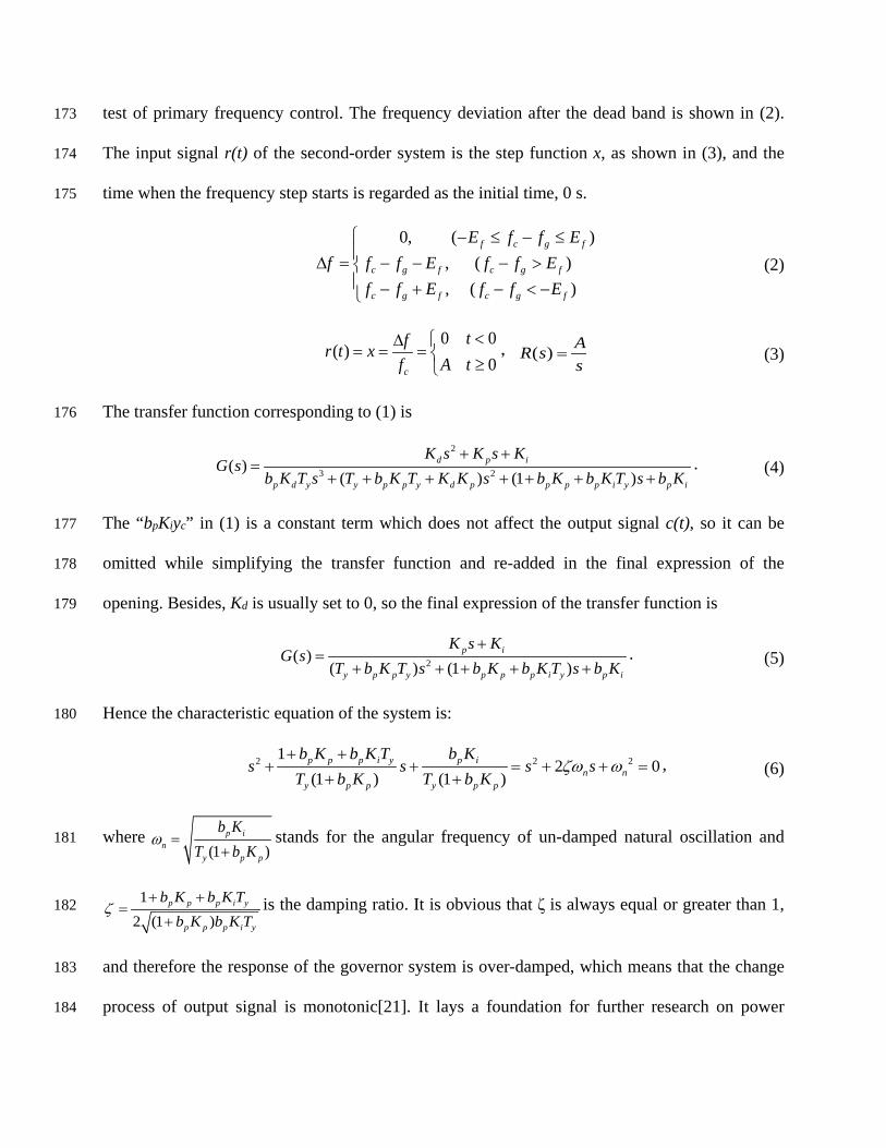
during the operation with smaller power output. The error in case 1 is slightly larger than which 164

of case 2, due to a much more rapid movement of opening and power. The slower the transient 165

process, the more accurate simulation. In general, it turns out to be a reliable model for further 166

simulation and research. 167

168

Fig. 5. Power response to a -0. 2Hz frequency step in case 1 Fig. 6. Power response to a +0.2 Hz frequency step in case 1

Fig. 7. Power response to a -0. 1 Hz frequency step in case 2 Fig. 8. Power response to a -0.3 Hz frequency step in case 2

169

5 Response time of primary frequency control 170

5.1 Time domain analytical solution of opening response 171

The time domain analytical solution of opening response is deduced based on the frequency step 172

test of primary frequency control. The frequency deviation after the dead band is shown in (2). 173

The input signal r(t) of the second-order system is the step function x, as shown in (3), and the 174

time when the frequency step starts is regarded as the initial time, 0 s. 175

0, ( ), ( ), ( )

f c g f

c g f c g f

c g f c g f

E f f Ef f f E f f E

f f E f f E

− ≤ − ≤∆ = − − − > − + − < −

(2)

0 0( )

0c

tfr t xA tf

<∆= = = ≥

， ( ) AR ss

= (3)

The transfer function corresponding to (1) is 176

2

3 2( )( ) (1 )

d p i

p d y y p p y d p p p p i y p i

K s K s KG s

b K T s T b K T K K s b K b K T s b K+ +

=+ + + + + + +

. (4)

The “bpKiyc” in (1) is a constant term which does not affect the output signal c(t), so it can be 177

omitted while simplifying the transfer function and re-added in the final expression of the 178

opening. Besides, Kd is usually set to 0, so the final expression of the transfer function is 179

2( )( ) (1 )

p i

y p p y p p p i y p i

K s KG s

T b K T s b K b K T s b K+

=+ + + + +

. (5)

Hence the characteristic equation of the system is: 180

2 2 212 0

(1 ) (1 )p p p i y p i

n ny p p y p p

b K b K T b Ks s s s

T b K T b Kζω ω

+ ++ + = + + =

+ +, (6)

where (1 )

p in

y p p

b KT b K

ω =+

stands for the angular frequency of un-damped natural oscillation and 181

12 (1 )

p p p i y

p p p i y

b K b K Tb K b K T

ζ+ +

=+

is the damping ratio. It is obvious that ζ is always equal or greater than 1, 182

and therefore the response of the governor system is over-damped, which means that the change 183

process of output signal is monotonic[21]. It lays a foundation for further research on power 184

quality. 185

186

By applying the transfer function (5) to a step yielding an expected unit change in output, i.e. (3) 187

with A=bp-1, we obtain the Laplace transform of the relative value of the opening signal at any 188

step, cf. (7). Then the relative value of the opening change process can be obtained from the 189

inverse Laplace transform, as shown in (8). To obtain the change process of actual opening, the 190

initial conditions (given opening yc and amplitude A/bp) should be considered, then the time 191

domain expression of opening response is acquired, see (9). 192

2C( )

( ) (1 )p i

y p p y p p p i y p i

K s Ks

s T b K T s b K b K T s b K+

= + + + + +

(7)

2 2( 1) ( 1)1( ) 1 )1 1

n ni y pt t

p p p i y p p p i y

K T Kc t e e

b K b K T b K b K Tζ ζ ω ζ ζ ω− − − − + −−

= − −+ − + −

(8)

( ) ( )cp

Ay t y c tb

= +

(9)

Equation (8) shows that the final steady-state value of the relative change process of opening is 1, 193

and the transient component consists of two exponential terms. Since ζ>1, and especially when 194

ζ>>1, we obtain that 2 1ζ ζ+ − >> 2 1ζ ζ− − . That is to say, for the two exponential terms in 195

(8), the latter attenuates far faster than the former. Hence the latter one can be ignored. The 196

simplified expression of time domain response is achieved by substituting the ωn and ζ by 197

governor parameters, as shown in (10). 198

11( ) 11

p i

p p

b Kt

b K

p p p i y

c t eb K b K T

−+= −

+ − (10)

The time when the monotonic output signal c(t) reaches the target value Δ (Δ is set to 90% 199

according to [17]) is 200

( )1

ln (1 ) 1p pp p p i y

p i

b Kt b K b K T

b K+

= − + − −∆ . (11)

Equation (11) is the formula for the opening response time of primary frequency control under 201

opening control. 202

203

If the parameter Ty is also ignored, equation (1) becomes first-order. The formula for the opening 204

response time can be obtained by applying the same method of Laplace inverse transform as 205

above: 206

( )1

ln (1 ) 1p pp p

p i

b Kt b K

b K+

= − + −∆ (12)

It is exactly the same as (11) when Ty = 0. Therefore (11) is a general formula including the case 207

when Ty is 0. 208

209

5.2 Simulation under different conditions 210

Simulations under different conditions are conducted in order to analyze the sensitivity of 211

response time with respect to the main parameters. All the simulation and analysis below is done 212

with case 1. The parameters of the simulation is set according to the test condition of the -0.2 Hz 213

frequency step in Section 4, except for the values in Table 1. A model without surge tank is 214

investigated and compared to analyze the influence of surge in upstream surge tank. More exactly, 215

in the model, the surge tank and the upstream pipeline before the tank are replaced by a reservoir, 216

see Fig. 9. Meanwhile, the upstream water level of the simplified model, which affects the water 217

head, is adjusted to ensure that the relation between guide vane opening and power remain the 218

same as in the original model. The simulation results are shown in Table 1. 219

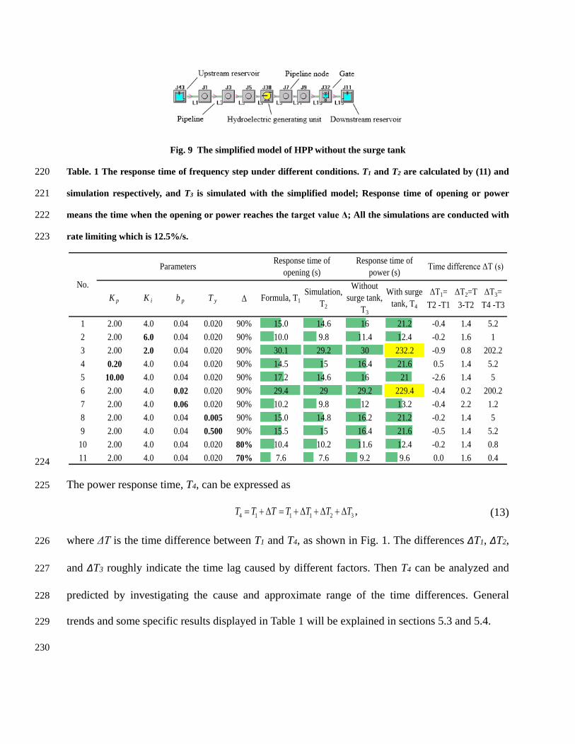
Fig. 9 The simplified model of HPP without the surge tank

Table. 1 The response time of frequency step under different conditions. T1 and T2 are calculated by (11) and 220

simulation respectively, and T3 is simulated with the simplified model; Response time of opening or power 221

means the time when the opening or power reaches the target value Δ; All the simulations are conducted with 222

rate limiting which is 12.5%/s. 223

1 2.00 4.0 0.04 0.020 90% 15.0 14.6 16 21.2 -0.4 1.4 5.22 2.00 6.0 0.04 0.020 90% 10.0 9.8 11.4 12.4 -0.2 1.6 13 2.00 2.0 0.04 0.020 90% 30.1 29.2 30 232.2 -0.9 0.8 202.24 0.20 4.0 0.04 0.020 90% 14.5 15 16.4 21.6 0.5 1.4 5.25 10.00 4.0 0.04 0.020 90% 17.2 14.6 16 21 -2.6 1.4 56 2.00 4.0 0.02 0.020 90% 29.4 29 29.2 229.4 -0.4 0.2 200.27 2.00 4.0 0.06 0.020 90% 10.2 9.8 12 13.2 -0.4 2.2 1.28 2.00 4.0 0.04 0.005 90% 15.0 14.8 16.2 21.2 -0.2 1.4 59 2.00 4.0 0.04 0.500 90% 15.5 15 16.4 21.6 -0.5 1.4 5.2

10 2.00 4.0 0.04 0.020 80% 10.4 10.2 11.6 12.4 -0.2 1.4 0.811 2.00 4.0 0.04 0.020 70% 7.6 7.6 9.2 9.6 0.0 1.6 0.4

No.

Parameters Response time of opening (s)

Response time of power (s)

K p K i b p

Time difference ΔT (s)

ΔT1= T2 -T1

ΔT2=T3-T2

ΔT3= T4 -T3

T y Δ Formula, T1Simulation,

T2

Without surge tank,

T3

With surge tank, T4

224

The power response time, T4, can be expressed as 225

4 1 1 1 2 3T T T T T T T= + ∆ = + ∆ + ∆ + ∆ , (13)

where ΔT is the time difference between T1 and T4, as shown in Fig. 1. The differences ΔT1, ΔT2, 226

and ΔT3 roughly indicate the time lag caused by different factors. Then T4 can be analyzed and 227

predicted by investigating the cause and approximate range of the time differences. General 228

trends and some specific results displayed in Table 1 will be explained in sections 5.3 and 5.4. 229

230

5.3 Effect of regulation system 231

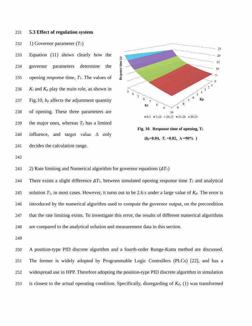
1) Governor parameter (T1) 232

Equation (11) shows clearly how the 233

governor parameters determine the 234

opening response time, T1. The values of 235

Ki and Kp play the main role, as shown in 236

Fig.10; bp affects the adjustment quantity 237

of opening. These three parameters are 238

the major ones, whereas Ty has a limited 239

influence, and target value Δ only 240

decides the calculation range. 241

242

2) Rate limiting and Numerical algorithm for governor equations (ΔT1) 243

There exists a slight difference ΔT1, between simulated opening response time T2 and analytical 244

solution T1, in most cases. However, it turns out to be 2.6 s under a large value of Kp. The error is 245

introduced by the numerical algorithm used to compute the governor output, on the precondition 246

that the rate limiting exists. To investigate this error, the results of different numerical algorithms 247

are compared to the analytical solution and measurement data in this section. 248

249

A position-type PID discrete algorithm and a fourth-order Runge-Kutta method are discussed. 250

The former is widely adopted by Programmable Logic Controllers (PLCs) [22], and has a 251

widespread use in HPP. Therefore adopting the position-type PID discrete algorithm in simulation 252

is closest to the actual operating condition. Specifically, disregarding of Kd, (1) was transformed 253

Fig. 10. Response time of opening, T1

(bp=0.04, Ty =0.02, Δ =90% )

to (14) through a standard first order difference method [22]: 254

1 2 12

1

2(1 ) (1 ) ( )k k k k ky p p p p p i y p i k c

k kp i k

y y y y yT b K b K b K T b K y yt t

x xK K xt

− − −

−

− + −+ + + + + −

∆ ∆−

= +∆

(14)

where △t is the time step and the subscript k stands for the current step. The fourth-order Runge-255

Kutta method is applied widely in all kinds of simulation software, and is for example available 256

in MATLAB. The brief principle is illustrated in Appendix B. 257

258

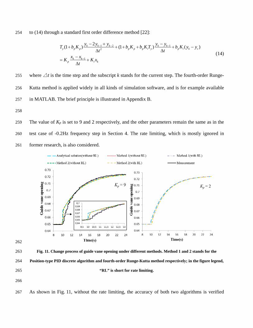
The value of Kp is set to 9 and 2 respectively, and the other parameters remain the same as in the 259

test case of -0.2Hz frequency step in Section 4. The rate limiting, which is mostly ignored in 260

former research, is also considered. 261

262

Fig. 11. Change process of guide vane opening under different methods. Method 1 and 2 stands for the 263

Position-type PID discrete algorithm and fourth-order Runge-Kutta method respectively; in the figure legend, 264

“RL” is short for rate limiting. 265

266

As shown in Fig. 11, without the rate limiting, the accuracy of both two algorithms is verified 267

because the results are consistent with the analytical solution. However there exits the rate 268

limiting in the actual case, and it will lead to a complex situation. To be specific, when the 269

proportional gain Kp is set to 9, the whole change process of opening obtained by Runge-Kutta 270

method is close to the analytical one and the opening speed is barely limited at the initial stage. 271

As a contrast, the position-type PID discrete algorithm shows a result which sharply diverges 272

from the analytical solution but has a good agreement with measurement data, since it is the 273

method adopted by the real governor. So a key problem is reflected that the actual opening 274

response does not coincide with the analytical solution. Normally the Runge-Kutta method is 275

regarded as a more accurate one, but it reduced the accuracy when modeling the normal governor. 276

While Kp is set to 2, the difference between the results of these two methods is small. In short, the 277

selection of algorithm should follow the actual built-in algorithm of the governor. The default 278

algorithm in some software, such as MATLAB, would probably bring the error especially when 279

Kp or the change rate of input signal is large. 280

281

5.4 Effect of water way system 282

The power response time T4 is normally greater than opening response time T2. The main cause is 283

the hydraulic character of the water way system, including the water hammer and surge in surge 284

tank. Moreover, the turbine efficiency is also a crucial factor which always affects the power 285

output, but it is relatively hard to analyze individually due to the serious nonlinear characteristic. 286

287

1) Water hammer (ΔT2) 288

Without the surge tank, the time lag between the response time of power and opening is ΔT2. 289

Water hammer is the main reason. Turbine efficiency and a minute change of water head can be 290

considered as secondary reasons. As shown in Fig. 5 and Fig. 6, the reverse power response due 291

to water hammer occurs immediately after the change of opening. It leads to a time delay of the 292

power response. 293

294

The key point is how much the water hammer delays the power response, which is rarely 295

discussed before. A similar discussion was conducted in [23], and this section makes a more 296

detailed investigation. The water hammer has a large influence during the first phase [24]. The 297

formula of reflection period of water hammer is 298

1

2ji

i i

LTa=

=∑ , (15)

where L is the length of a pipeline, a stands for the wave velocity of water hammer, i represents a 299

specific pipeline and j is the number of pipelines between the turbine and reservoir (or surge tank). 300

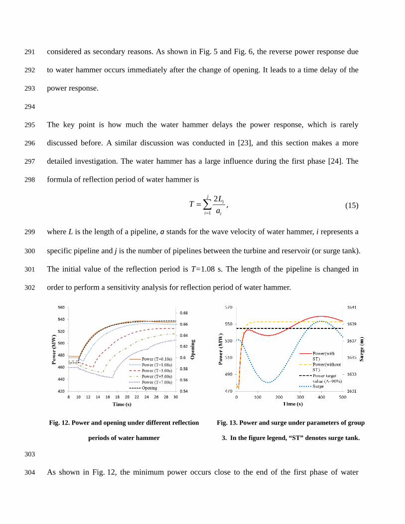
The initial value of the reflection period is T=1.08 s. The length of the pipeline is changed in 301

order to perform a sensitivity analysis for reflection period of water hammer. 302

303

As shown in Fig. 12, the minimum power occurs close to the end of the first phase of water 304

Fig. 12. Power and opening under different reflection

periods of water hammer

Fig. 13. Power and surge under parameters of group

3. In the figure legend, “ST” denotes surge tank.

hammer, and it takes an additional short time for the power to return to the initial value. In other 305

words, the water hammer leads to a delay time Tdelay which is at least as long as a reflection 306

period T. However the ΔT2 is hard to predict precisely and may even be less than T, owing to the 307

various factors such as the turbine efficiency and water head. Nevertheless the rough value of ΔT2 308

can be estimated according to T, because there is only a tiny difference between these two values. 309

310

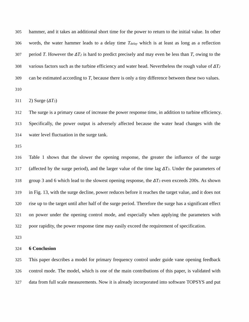
2) Surge (ΔT3) 311

The surge is a primary cause of increase the power response time, in addition to turbine efficiency. 312

Specifically, the power output is adversely affected because the water head changes with the 313

water level fluctuation in the surge tank. 314

315

Table 1 shows that the slower the opening response, the greater the influence of the surge 316

(affected by the surge period), and the larger value of the time lag ΔT3. Under the parameters of 317

group 3 and 6 which lead to the slowest opening response, the ΔT3 even exceeds 200s. As shown 318

in Fig. 13, with the surge decline, power reduces before it reaches the target value, and it does not 319

rise up to the target until after half of the surge period. Therefore the surge has a significant effect 320

on power under the opening control mode, and especially when applying the parameters with 321

poor rapidity, the power response time may easily exceed the requirement of specification. 322

323

6 Conclusion 324

This paper describes a model for primary frequency control under guide vane opening feedback 325

control mode. The model, which is one of the main contributions of this paper, is validated with 326

data from full scale measurements. Now it is already incorporated into software TOPSYS and put 327

into practical application. 328

329

Aiming at the response time of guide vane opening, a time domain analytical solution for opening 330

response and a formula of response time, of which the main variables are governor parameters, 331

are derived. The time difference ΔT, between the power response time and the analytical response 332

time of opening, is mainly affected by rate limiting and numerical algorithm (ΔT1), water hammer 333

(ΔT2) and surge (ΔT3). However, the most direct and effective method is still adjusting the 334

governor parameters. Especially for a HPP without surge tank, the ΔT changes within a small 335

range, so the formula of opening response time can also help to predict the power response and 336

supply a flexible guidance of parameter tuning. 337

338

Furthermore, this research can be extended in the aspects below: a more complex frequency 339

deviation should be analyzed. The turbine efficiency is a key factor which needs to be further 340

investigated individually. This research only focus on the control mode with guide vane opening 341

feedback, but power droop or more advanced mode should also be studied. Such improvements 342

will possibly make a more comprehensive description and understanding for the dynamic 343

response of hydroelectric generating units in primary frequency control. 344

345

Acknowledgements 346

The authors thank the China Scholarship Council (CSC) and StandUp for Energy. The authors 347

also acknowledge the support from the National Natural Science Foundation of China under 348

Grant No. 51379158 and No. 51039005. The research presented was also carried out as a part of 349

"Swedish Hydro power Centre - SVC". SVC has been established by the Swedish Energy Agency, 350

Elforsk and Svenska Kraftnät together with Luleå University of Technology, KTH Royal Institute 351

of Technology, Chalmers University of Technology and Uppsala University (www.svc.nu). 352

353

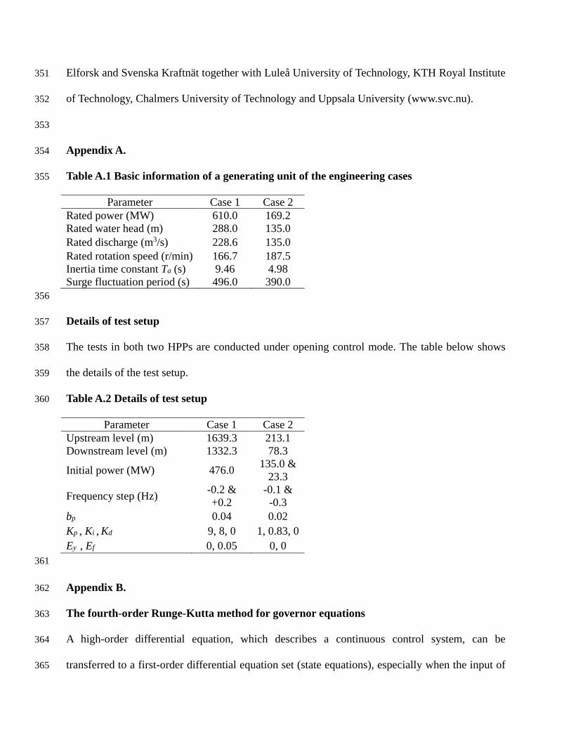
Appendix A. 354

Table A.1 Basic information of a generating unit of the engineering cases 355

Parameter Case 1 Case 2 Rated power (MW) 610.0 169.2 Rated water head (m) 288.0 135.0 Rated discharge (m3/s) 228.6 135.0 Rated rotation speed (r/min) 166.7 187.5 Inertia time constant Ta (s) 9.46 4.98 Surge fluctuation period (s) 496.0 390.0 356

Details of test setup 357

The tests in both two HPPs are conducted under opening control mode. The table below shows 358

the details of the test setup. 359

Table A.2 Details of test setup 360

Parameter Case 1 Case 2 Upstream level (m) 1639.3 213.1 Downstream level (m) 1332.3 78.3

Initial power (MW) 476.0 135.0 & 23.3

Frequency step (Hz) -0.2 & +0.2

-0.1 & -0.3

bp 0.04 0.02 Kp , Ki , Kd 9, 8, 0 1, 0.83, 0 Ey , Ef 0, 0.05 0, 0 361

Appendix B. 362

The fourth-order Runge-Kutta method for governor equations 363

A high-order differential equation, which describes a continuous control system, can be 364

transferred to a first-order differential equation set (state equations), especially when the input of 365

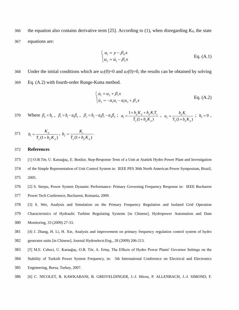
the equation also contains derivative term [25]. According to (1), when disregarding Kd, the state 366

equations are: 367

1 0

2 1 1

u y xu u x

ββ

= − = −

Eq. (A.1)

Under the initial conditions which are u1(0)=0 and u2(0)=0, the results can be obtained by solving 368

Eq. (A.2) with fourth-order Runge-Kutta method. 369

1 2 1

2 2 1 1 2 2

u u xu a u a u x

ββ

= + = − − +

Eq. (A.2)

Where 0 0bβ = , 1 1 1 0b aβ β= − , 2 2 1 1 2 0b a aβ β β= − − ; 1

1(1 )

p p p i y

y p p

b K b K Ta

T b K+ +

=+

, 2

yT (1 )p i

p p

b Ka

b K=

+; 0 0b = , 370

1 (1 )p

y p p

Kb

T b K=

+,

2 (1 )i

y p p

KbT b K

=+

. 371

References 372

[1] O.B.Tör, U. Karaağaç, E. Benlier, Step-Response Tests of a Unit at Atatürk Hydro Power Plant and Investigation 373

of the Simple Representation of Unit Control System in: IEEE PES 36th North American Power Symposium, Brazil, 374

2005. 375

[2] S. Sterpu, Power System Dynamic Performance: Primary Governing Frequency Response in: IEEE Bucharest 376

Power Tech Conference, Bucharest, Romania, 2009. 377

[3] S. Wei, Analysis and Simulation on the Primary Frequency Regulation and Isolated Grid Operation 378

Characteristics of Hydraulic Turbine Regulating Systems [in Chinese], Hydropower Automation and Dam 379

Monitoring, 33 (2009) 27-33. 380

[4] J. Zhang, H. Li, H. Xie, Analysis and improvement on primary frequency regulation control system of hydro 381

generator units [in Chinese], Journal Hydroelectr.Eng., 28 (2009) 206-213. 382

[5] M.E. Cebeci, U. Karaağaç, O.B. Tör, A. Ertaş, The Effects of Hydro Power Plants' Governor Settings on the 383

Stability of Turkish Power System Frequency, in: 5th International Conference on Electrical and Electronics 384

Engineering, Bursa, Turkey, 2007. 385

[6] C. NICOLET, B. KAWKABANI, B. GREIVELDINGER, J.-J. Hérou, P. ALLENBACH, J.-J. SIMOND, F. 386

AVELLAN, Turbine Speed Governor Parameters Validation in Islanded Production, in: 2nd IAHR International 387

Meeting of the Workgroup on Cavitation and Dynamic Problems in Hydraulic Machinery and Systems Timisoara, 388

Romania 2007. 389

[7] J. Zhang, H. Li, H. Xie, Study on the stability of primary frequency regulating system of hydroelectric units [in 390

Chinese], Journal Hydroelectr.Eng., 29 (2010) 208-214. 391

[8] A. Khodabakhshian, R. Hooshmand, A new PID controller design for automatic generation control of hydro 392

power systems, International Journal of Electrical Power and Energy Systems, 32 (2010) 375-382. 393

[9] P. Hušek, PID controller design for hydraulic turbine based on sensitivity margin specifications, International 394

Journal of Electrical Power and Energy Systems, 55 (2014) 460-466. 395

[10] M. Hanmandlu, H. Goyal, Proposing a new advanced control technique for micro hydro power plants, 396

International Journal of Electrical Power and Energy Systems, 30 (2008) 272-282. 397

[11] K.C. Divya, P.S.N. Rao, A simulation model for AGC studies of hydro-hydro systems, International Journal of 398

Electrical Power and Energy Systems, 27 (2005) 335-342. 399

[12] S.P. Mansoor, D.I. Jones, D.A. Bradley, F.C. Aris, G.R. Jones, Reproducing oscillatory behaviour of a 400

hydroelectric power station by computer simulation, Control Engineering Practice, 8 (2000) 1261-1272. 401

[13] D.I. Jones, S.P. Mansoor, F.C. Aris, G.R. Jones, D.A. Bradley, D.J. King, A standard method for specifying the 402

response of hydroelectric plant in frequency-control mode, Electr. Power Syst. Res., 68 (2004) 19-32. 403

[14] J. Andrade, E. Júnior, L. Ribeiro, Using genetic algorithm to define the governor parameters of a hydraulic 404

turbine, in: 25th IAHR Symposium on Hydraulic Machinery and Systems, Timişoara, Romania, 2010. 405

[15] C.S. Li, J.Z. Zhou, Parameters identification of hydraulic turbine governing system using improved gravitational 406

search algorithm, Energ Convers Manage, 52 (2011) 374-381. 407

[16] H. Bao, J. Yang, L. Fu, Study on Nonlinear Dynamical Model and Control Strategy of Transient Process in 408

Hydropower Station with Francis turbine, in: Asia-Pacific Power and Energy Engineering Conference 2009, Wuhan, 409

2009. 410

[17] C.E. Council, DL/T 1040-2007, in, 2007. 411

[18] E.N.o.T.S.O.f. Electricity, ENTSO-E Operation Handbook, Policy 1 (2009): Load-Frequency Control and 412

Performance, in, 2009. 413

[19] Statnett, Funksjonskrav i kraftsystemet 2012 [in Norwegian], in, 2012. 414

[20] S. Kraftnät, Regler för upphandling och rapportering av primärreglering FCR-N och FCR-D (från 16 november 415

2012) [in Swedish], in, 2012. 416

[21] M. Driels, Linear Control Systems Engineering Mcgraw-Hill College, New York, 1995. 417

[22] T. Zhou, Y. Wu, Technology of hydraulic turbine governor [in Chinese], China WaterPower Press, Beijing, 2010. 418

[23] C. Nicolet, B. Greiveldinger, J.J. Hérou, B. Kawkabani, P. Allenbach, J.-J. Simond, F. Avellan, High-Order 419

Modeling of Hydraulic Power Plant in Islanded Power Network[J], IEEE Transactions on Power Systems, 22 (2007) 420

1870-1880. 421

[24] W. Yang, J. Yang, Research on the volute pressure in start-up process of hydroelectric generating units, IOP 422

Conference Series: Earth and Environmental Science, (2012). 423

[25] K. Ogata, Modern Control Engineering (Fourth Edition), Tsinghua University Press, Beijing, 2006. 424

425

426