February 2005

NASA/TM-2005-213518

Magnetic Field Response Measurement

Acquisition System

Stanley E. Woodard

Langley Research Center, Hampton, Virginia

Bryant D. Taylor

Swales Aerospace Corporation, Hampton, Virginia

Qamar A. Shams and Robert L. Fox

Langley Research Center, Hampton, Virginia

The NASA STI Program Office . . . in Profile

Since its founding, NASA has been dedicated

to the advancement of aeronautics and space

science. The NASA Scientific and Technical

Information (STI) Program Office plays a key

part in helping NASA maintain this important

role.

The NASA STI Program Office is operated by Langley

Research Center, the lead center for NASA’s scientific

and technical information. The NASA STI Program

Office provides access to the NASA STI Database, the

largest collection of aeronautical and space science STI

in the world. The Program Office is also NASA’s

institutional mechanism for disseminating the results of

its research and development activities. These results are

published by NASA in the NASA STI Report Series,

which includes the following report types:

• TECHNICAL PUBLICATION. Reports of

completed research or a major significant phase

of research that present the results of NASA

programs and include extensive data or

theoretical analysis. Includes compilations of

significant scientific and technical data and

information deemed to be of continuing reference

value. NASA counterpart of peer-reviewed

formal professional papers, but having less

stringent limitations on manuscript length and

extent of graphic presentations.

• TECHNICAL MEMORANDUM. Scientific and

technical findings that are preliminary or of

specialized interest, e.g., quick release reports,

working papers, and bibliographies that contain

minimal annotation. Does not contain extensive

analysis.

• CONTRACTOR REPORT. Scientific and

technical findings by NASA-sponsored

contractors and grantees.

• CONFERENCE PUBLICATION. Collected

papers from scientific and technical

conferences, symposia, seminars, or other

meetings sponsored or co-sponsored by NASA.

• SPECIAL PUBLICATION. Scientific,

technical, or historical information from NASA

programs, projects, and missions, often

concerned with subjects having substantial

public interest.

• TECHNICAL TRANSLATION. English-

language translations of foreign scientific and

technical material pertinent to NASA’s mission.

Specialized services that complement the STI

Program Office’s diverse offerings include creating

custom thesauri, building customized databases,

organizing and publishing research results ... even

providing videos.

For more information about the NASA STI Program

Office, see the following:

• Access the NASA STI Program Home Page at

http://www.sti.nasa.gov

• E-mail your question via the Internet to

help@sti.nasa.gov

• Fax your question to the NASA STI Help Desk

at (301) 621-0134

• Phone the NASA STI Help Desk at

(301) 621-0390

• Write to:

NASA STI Help Desk

NASA Center for AeroSpace Information

7121 Standard Drive

Hanover, MD 21076-1320

February 2005

NASA/TM-2005-213518

Magnetic Field Response Measurement

Acquisition System

Stanley E. Woodard

Langley Research Center, Hampton, Virginia

Bryant D. Taylor

Swales Aerospace Corporation, Hampton, Virginia

Qamar A. Shams and Robert L. Fox

Langley Research Center, Hampton, Virginia

Available from:

NASA Center for AeroSpace Information (CASI)

7121 Standard Drive

Hanover, MD 21076-1320

(301) 621-0390

National Technical Information Service (NTIS)

5285 Port Royal Road

Springfield, VA 22161-2171

(703) 605-6000

Acknowledgments

The authors thank the following individuals for their support: Dr. R. G. Bryant, Dr. L. G.

Horta, Dr. H. M. Adelman, Mr. R. L. Chattin, R. C. Webster, and R. W. Edwards of

NASA Langley Research Center; Mr. Rashaan Campbell of Morehouse College and

Georgia Institute of Technology.

1

Magnetic Field Response Measurement Acquisition System

Stanley E. Woodard, Bryant D. Taylor Qamar A. Shams and Robert L. Fox

NASA Langley Research Center

Hampton, VA 23681

This paper presents a measurement acquisition method that alleviates many shortcomings of traditional measurement systems. The shortcomings are a finite number of measurement channels, weight penalty associated with measurements, electrical arcing, wire degradations due to wear or chemical decay, and the logistics needed to add new sensors. Wire degradation has resulted in aircraft fatalities and critical space launches being delayed. The key to this method is the use of sensors designed as passive inductor-capacitor circuits that produce magnetic field responses. The response attributes correspond to states of physical properties for which the sensors measure. Power is wirelessly provided to the sensor by using Faraday induction. An antenna produces a time-varying magnetic field used to power the sensor and receive the magnetic field response of the sensor. An interrogation system for discerning changes in the sensor response frequency, resistance, and amplitude has been developed and is presented herein. Multiple sensors can be interrogated using this method. The method eliminates the need for a data acquisition channel dedicated to each sensor. The method does not require the sensors to be near the acquisition hardware. Methods of developing magnetic field response sensors and the influence of key parameters on measurement acquisition are discussed. Examples of magnetic field response sensors and their respective measurement characterizations are presented. Implementation of this method on an aerospace system is discussed.

2

Introduction Throughout aviation and space history, measurement acquisition has relied upon traditional methods of using wires connected to sensors to supply power to the sensors and to obtain measurements from the sensors. Newer methods using transceivers for wireless measurements require the sensors to be connected to a processor that is connected to a transceiver. An example of a wireless system is that found in Ref. 1. Another method of acquiring measurements is the use of radio frequency identification (RFID) tags. RFID systems eliminate the need for physical connection to an external power source but require physical connection to a silicon chip. Many harsh environments (e.g., gas, chemical, thermal) prohibit the use of silicon-based processors. Furthermore, the distance for which RFID can be interrogated is approximately 15 cm in the 1-25 MHz frequency range that is available for aviation use.1 Logistically, much can be gained from implementation of sensors which have no physical connection to a power source, processor, or data acquisition equipment. Eliminating wiring for acquiring measurements can alleviate potential hazards associated with wires. Wiring hazards include damaged wires becoming ignition sources due to arcing. Wire damage can result from wire fraying, chemical degradation of wire insulation, wire splaying, and wire chaffing (e.g., under a clamp). Many of the aforementioned methods of wire damage have resulted in critical spacecraft launch delays or aircraft fatalities. Wires within combustible fluids (e.g., fuel tanks) also present potential hazards. Either an electrical short or lightning exposes the fluid to excessive voltage. In 1999, wire damage was discovered in all four space shuttles2. The damage was caused by ground servicing equipment. An electrical short halted the launch of the Columbia whose payload was the Chandra X-Ray Observatory. The short triggered inspections on all four shuttles. A supply mission to the then unstaffed International Space Station was also delayed so that all wire damage discovered could be repaired. The repairs reduced the number of missions in 1999 to three, the fewest since 1988.2 In 2002, the launch of a replacement Global Positioning Satellite aboard a Delta 2 rocket was delayed to allow engineers to study the wiring harness. The study resulted from problems discovered from another rocket at the manufacturing facility3. The aforementioned cases of wiring problems resulted in delayed missions but no loss of life. Two recent major aircraft accident investigations indicate that wiring faults were the source of the fatalities.4-5 On July 17, 1996, Trans World Airlines, Inc. (TWA) Flight 800, crashed in the Atlantic Ocean near East Moriches, New York. The TWA Flight 800 in-flight breakup was initiated by a fuel/air explosion in the center wing fuel tank. All 230 people aboard the Boeing 747-131 were killed. The National Transportation Safety Board determined that the probable cause of the accident was an explosion of the center wing fuel tank, resulting from ignition of the flammable fuel/air mixture in the tank. The most likely source of ignition was a short circuit outside of the fuel tank that allowed excessive voltage to enter the tank through the fuel quantity indication system electrical wiring.4 Damaged wiring was also determined to be the cause of the another major fatal accident. On September 2, 1998, approximately 53 minutes after the Swissair Flight 111 departure from New York and at flight level 330, the flight crew detected an abnormal odor in the cockpit. After detecting visible smoke, the crew diverted to Halifax International Airport. While preparing to land, a fire spread above the ceiling in the front area of the aircraft. Less than 20 minutes after the odor was first detected, the flight crashed into the ocean off the coast of Nova Scotia. All 229 people onboard the McDonnell Douglas MD-11

3

were killed. The Transportation Safety Board of Canada determined that the most likely cause of the fire was a wire arcing event.5 This paper presents a measurement acquisition system that uses magnetic fields to power sensors and to acquire the measurement from sensors. The sensors are not connected to a power source, silicon-based processor, or any data acquisition equipment. The inherent design of the sensor and the means of powering the sensors eliminate the potential for arcing. The measurement acquisition system and sensors are extremely lightweight. The system can greatly increase the number of measurements performed while alleviating the weight associated with many science and engineering measurements. Measurement complexity and probability of failure is greatly reduced. Sensors are designed as passive inductor-capacitor circuits that produce magnetic field responses when electrically excited. The response attributes correspond to states of physical properties for which the sensors measure. An antenna produces a time-varying magnetic field that remotely powers all sensors (via Faraday induction).6,7 The magnetic field responses of the inductors serve as a means of communication with the measurement acquisition system. The antenna receives the magnetic field response from each sensor, thus the system is wireless. The use of magnetic fields for powering the sensors and for acquiring the measurements from the sensors eliminates the need for physical connection from the sensor to a power source and to data acquisition equipment. Once electrically excited, the sensors have very low voltage. If a short does occur in the sensor, the sensor cannot be activated because a completed circuit is needed for Faraday induction. Hence, electrical arcing is prevented. The system also eliminates the need to have a data acquisition channel dedicated to each sensor. The method greatly reduces the difficulty of implementing a measurement system. New measurements only require that the new sensors be placed within the magnetic field of the interrogating antenna(s) and that the processor gets the appropriate calibration data. Many of the sensors and interrogating antennas can be directly placed on the vehicles using metallic film deposition methods providing further weight reduction. Because the functionality of the sensors is based upon magnetic fields, they have potential use at cryogenic temperatures, extremely high temperatures, harsh chemical environments, and radiative environments. Furthermore, the method allows acquiring measurements that were previously unattainable or logistically difficult because there was no practical means of getting power and data acquisition electrical connections to a sensor. The system eliminates many “wire” issues such as weight, degradation, aging, and wear. To date, sensors that have been developed using this concept are position, dielectric level (e.g., fluid, level, or, solid, particle, level), load (shear, axial, torsion), angular orientation, material phase transition, moisture, various chemical exposure, rotation/displacement measurements, bond separation, proximity sensing, contact, pressure, strain, and crack detection. Many examples of magnetic field response sensors and their respective means of interrogation are in the literature.8-16 The limitation of the interrogation methods is the separation distance between the sensor and the interrogator. When a single antenna is used, interrogation distance is no more than 0.15 m. Using two antennas, interrogation can occur between the antennas when they are separated by 1.5 m.11 The key to practical use in vehicles is increased interrogation

4

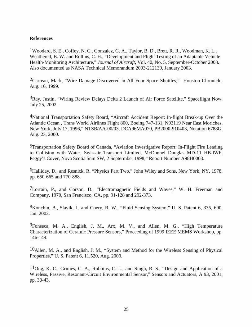
antenna-sensor separation distance and to facilitate multiple measurements whose dynamic characteristics affect different attributes of the sensor’s magnetic field response.16 The method demonstrated herein has interrogation distance of 2.7 m using 1.0 W and 3.3 m using 1.5 W of power when separate transmission and receiving antennas are used. An interrogation distance of 0.6 m is achieved when using a single antenna with 0.1 W applied power. The measurement system presented herein can be integrated into other systems to increase their capabilities. The measurement system can be installed during any phase of a vehicle’s life and it is less costly to install new sensors than the traditional method of wiring a sensor to acquisition equipment. Such a system can be used to implement measurements that were not envisioned during design of a system but identified as needed during testing or operation of the system. This paper discusses the measurement acquisition system and the class of sensors that the system interrogates. Following the introduction, a measurement interrogation method capable of discerning changes to all magnetic field response attributes will be presented. Examples of the sensors and their respective characterization test results are presented next, followed by methods of developing magnetic field response sensors. Implementation of this method on aerospace systems will then be discussed. Appendix A discusses the influence of critical physical attributes to measurements. Measuring sensor resistive variations is discussed in Appendix B. Overview of Measurement Acquisition Method Capacitor geometric, capacitor dielectric (e.g., due to the presence of chemical species or due to a material phase transition), inductor geometric, or inductor permeability changes of a sensor will result in magnetic field response frequency change. Any resistive change will result in a response bandwidth change. When a sensor’s inductor comes in proximity to conductive material, energy is lost in the sensor due to eddy currents being produced in the conductive material. As the sensor is brought closer to the material, the response amplitude decreases while the response frequency increases. This effect can be used to determine proximity to conductive surfaces. If capacitance and inductance are fixed, a sensor’s orientation or position with respect to an interrogating antenna can be measured using the sensor response amplitude (provided that only one parameter changes). A sensor of fixed inductance and capacitance can be used for measuring temperature. Temperature variations alter the intrinsic resistance of the sensors. The response bandwidth resulting from resistance change can be used to determine temperature. The interrogation system described herein allows for acquiring measurements from any magnetic field response sensor developed to exploit the aforementioned phenomena. The system also allows for autonomous sensor interrogation, analysis of collected response to value of physical state, and comparison of current measurements with prior measurements to produce dynamic measurements. The interrogation system has two key features: the hardware for producing a varying magnetic field at a prescribed frequency and algorithms for controlling the magnetic field produced and analyzing sensor responses. Fig. 1 shows a schematic of the measurement acquisition method for magnetic field response sensors using a single antenna and multiple magnetic field response sensors. The components of the measurement system are an antenna for transmitting and receiving magnetic fields, a processor for regulating the magnetic field transmission and reception, software for control of the

5

antenna and for analyzing the responses received, and magnetic field response sensors. The processor modulates the input signal to the antenna to produce either a broadband time-varying magnetic field or a single frequency magetic field. The transmitted magnetic field creates an electrical current in each passive inductor-capacitor, L-C, circuit as a result of Faraday induction.

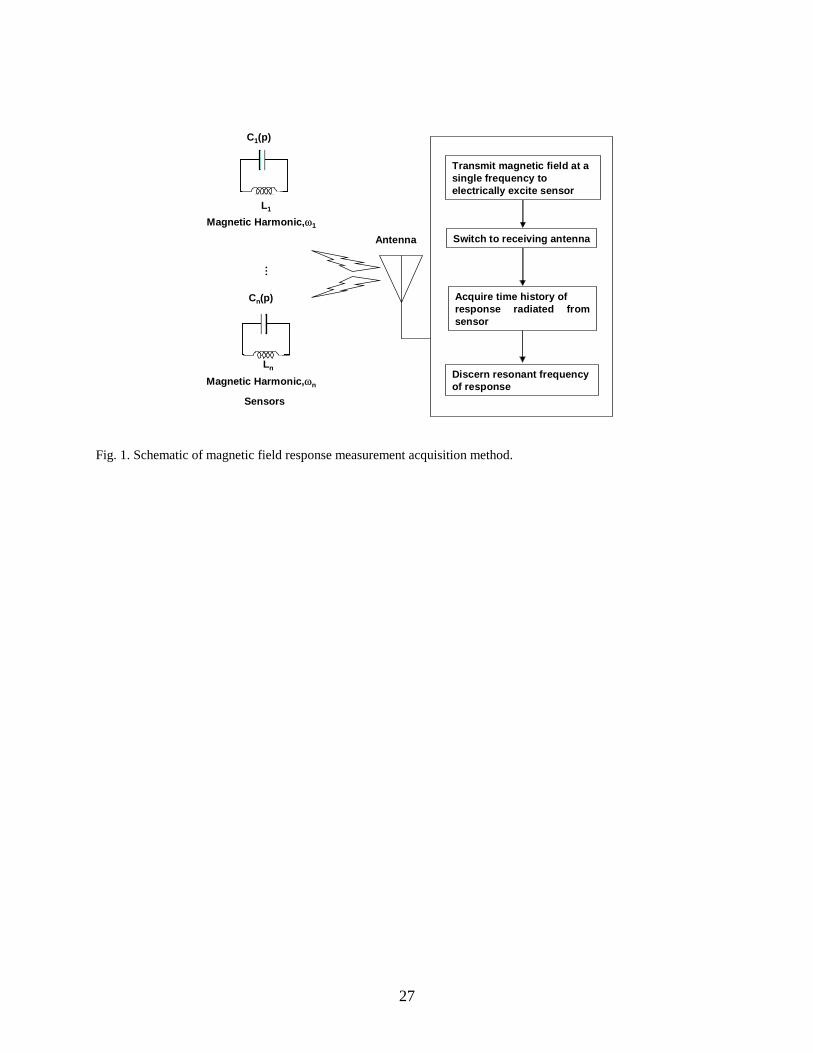
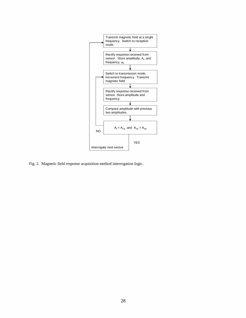
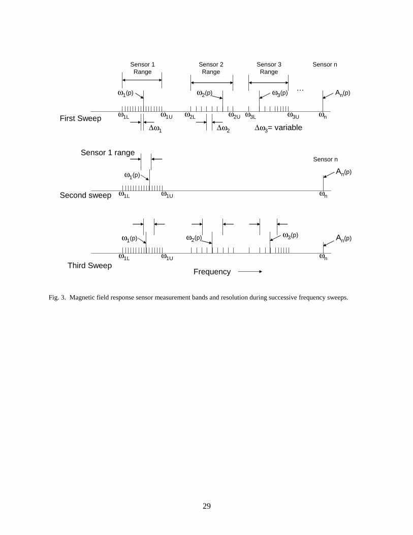
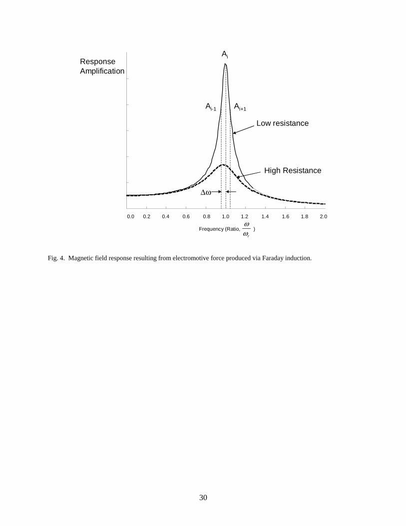
Each circuit will produce a magnetic field response with resonant frequency, ω(p), and amplitude, A(p), that are dependent upon the physical property, p. The oscillation occurs as the energy is harmonically transferred between the inductor (as magnetic energy) and capacitor (as electrical energy). When the energy is in the inductors, the magnetic fields produced are single harmonics whose frequencies are the respective sensor resonant frequencies. A receiving antenna is used to receive the magnetic responses produced by the inductors. The receiving antenna can be the same antenna used to produce the initial transmission of the magnetic field received by the sensor or another antenna can be used. When the same antenna is used, it must be switched from a transmitting antenna to a receiving antenna. A microprocessor is used to identify the response attributes received by the antenna. The measured response attributes are then correlated to measurement of physical states. The interrogation logic is presented in Fig. 2. The interrogation method is that of a scan-listen-compare technique.16 A single frequency is transmitted from the transmission antenna. The sensor is electrically excited, thus causing its inductor to produce a magnetic response. A receiving antenna listens to the inductor response and compares it to the previous inductor response. Each sensor has a dedicated frequency partition (measurement band). A single antenna sweep covers measurement bands for all sensors. Examples of sensor measurement bands and the sampling resolution for n sensors are shown in Fig. 3 for successive frequency sweeps. Each sensor has a frequency resolution (∆ω) that corresponds to a measurement resolution of the physical state. The sweep of individual frequencies is used because it concentrates all energy used to excite the sensor at a single frequency producing a higher signal-to-noise ratio than would result from a broadband transmission. Fig. 4 depicts the sensor response amplitude as the excitation frequency approaches the sensor resonant frequency. Transmission and receiving antennas can be used or a single switching antenna can be used. Using two antennas provides a larger volumetric swath at which measurements can be taken that is approximately double that of a single antenna. The interrogation procedure will be presented for a single sensor. The procedure is:

1. At the lower limit of a predetermined range, a harmonic magnetic field, ωi = ωL, is transmitted for a predetermined length of time and then the transmission mode is switched off (i.e., the transmission antenna is turned off if two antennas are used or if a single antenna is used, it ceases transmission).

2. The receiving mode is then turned on (i.e., the receiving antenna is turned on if two

antennas are used or if a single antenna is used, it begins receiving). The received response from the sensor is rectified to determine its amplitude. The amplitude, Ai, and frequency, ωi, are stored in memory.

3. The receiving mode is turned off and the transmission mode is turned on. The

transmitted harmonic magnetic field is then shifted by a predetermined amount, ωi+1 = ωi +

6

∆ω. The frequency shift, ∆ω, is based upon the desired sensor frequency resolution). The harmonic is transmitted for a predetermined length of time and then the transmission mode is turned off.

4. The receiving mode is then turned on. The received response from the sensor is rectified

to determine its amplitude. The amplitude, Ai+1, and frequency, ωi+1, are stored in memory.

5. The current amplitude, Ai+1, is compared to the two previously stored amplitudes, Ai and Ai-1. If the previous amplitude, Ai, is greater than the current amplitude, Ai+1, and if the previous amplitude is greater than the amplitude prior to it, Ai-1, the previous amplitude, Ai, is the peak amplitude. The peak amplitude occurs when the excitation frequency is equal to the resonant frequency of the sensor. The peak amplitude, Ai, and the corresponding frequency, ωi, are cataloged for the sensor for the current frequency sweep. These values can be compared to the values acquired during the next sweep. If an amplitude peak has not been identified, then steps 3 - 5 are repeated.

6. If an amplitude peak has been identified, the transmission frequency is changed to the

lower bound of the next sensor. Steps 1-5 are performed for that sensor. The initial frequency sweep can be used to identify and catalog all resonant peaks associated with all sensors within the antenna’s range of interrogation (Fig. 3). The sweep duration must be less than half the Nyquist period of the measured physical state with the highest frequency. For example, if one sensor is measuring vibrations of less than 30 Hz and other measured states have rates of change less than 30 Hz, then the sweeps must be done at a rate of 60 Hz or greater. The cataloged amplitudes and resonant frequencies for all sensors can be used to reduce the sweep time for successive sweeps. For example, the next sweep to update each resonant frequency can start and end at a predetermined proximity (i.e., narrowing the measurement range) to the cataloged resonant and then skip to the next resonant (Fig. 3). Narrowing the interrogation frequency bounds within a measurement band could be used as a means of increasing the sweep rate. Not all measurement bands need to be interrogated during successive sweeps. If a physical state does not change rapidly or is somewhat quasistatic, it may not be necessary to collect its measurement at each sweep. In Fig. 3, only two sensors are interrogated for the second sweep. Dynamic measurements can also be produced by comparing variation in frequencies and amplitudes of the current sweep with those of the prior sweeps. For example, if capacitance and inductance are fixed and if the circuit follows a known trajectory (e.g., displacement of a lever), the change in circuit position can be determined by comparing the amplitudes (Ai) variations of successive sweeps (as shown by the last sensor). Similarly, dynamic strain measurements can be determined by comparing the frequencies of successive measurements. The sensor responses are superimposed. The sensors are designed (Fig. 3) such that their range of measurement frequencies does not overlap but the ranges are within a frequency range of the antenna. The range of resonant frequencies corresponds to the range of physical property values that can be measured. An example would be that the lower frequency in the measurement band, ωL, would correspond to the lower limit of a strain measurement. This method allows for any

7

number of sensors within the range of the antennas to be interrogated. It should be noted that the discrete frequencies need not be evenly spaced in any measurement band. The higher the number of discrete frequencies within a band, the higher sensor resolution. Basically, the objective of the aforementioned methods is to identify the inflection point of each sensor’s magnetic field response. Once peak amplitude has been detected, the peak amplitude and frequency are stored and then the next partition is examined. After the last partition is examined, a new sweep is started. At each transmitted frequency, ωi+1, the current amplitude, Ai+1, and the previous two amplitudes (Ai and Ai-1) and their respective frequencies are stored. The amplitudes are compared to identify the peak amplitude. The frequency at which the amplitude peak occurs is the resonant frequency. The initial sweep is to ascertain all resonant frequencies and their corresponding amplitudes. Frequencies and amplitude values of successive sweeps can be compared to previous sweeps to ascertain if there is any change to measured property or if the antenna has moved with respect to the antenna. If the physical state has changed, the resonant frequency will be different from prior sweep. If a sensor has moved with respect to the antenna, the amplitudes will be different (frequency will remain constant). The magnitude and sign of the difference can be used to determine how fast the sensor is moving and whether the sensor is moving toward the antenna or away from the antenna. The interrogation method can be extended to allow for resistive measurements. Once the resonant frequency and its respective amplitude for a sensor have been identified, the amplitude at a fixed frequency shift prior to the resonant is then acquired. The resistance is inversely proportional to the difference of the amplitudes. The justification for such a technique appears in Appendix B, “Measuring Sensor Resistive Variations.” The measurement system presented herein is simple to implement in existing vehicles or plants. Once installed, it is easy to add new measurements. No wiring is required. All that is required for each sensor is a unique frequency partition and a frequency/measurement correlation table. Measurements can be acquired when the sensor is embedded in material that is transmissive to the magnetic field energy. For electrically conductive material, the capacitor is electrically insulated and then embedded. The inductor is placed away from the surface of the conductive material and then electrically connected to the conductor. Inductors, antennas, and some capacitor types can be developed as metallic foils or placed via metal deposition techniques onto nonconductive surfaces (e.g., a structural component or a thin-film) thus making them nonobtrusive. Metal deposition can be used to add sensors or antennas to a vehicle during manufacturing. Other adavantages of the measurement system are that multiple sensors can be interrogated using a single data acquisition channel (used for antenna). No specific orientation of sensor with respect the antenna used to excite the sensor is required except that they cannot be 90 deg to each other. No line-of-sight is required between antenna and sensor.

8

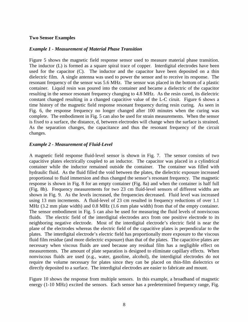
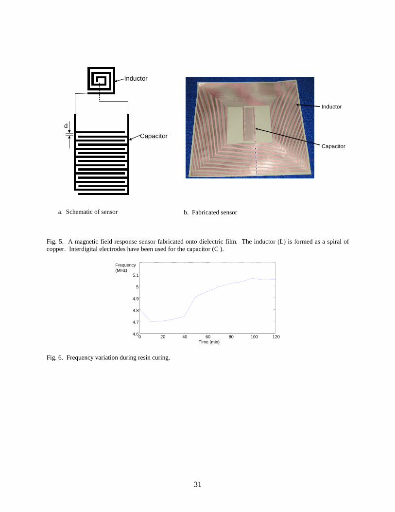
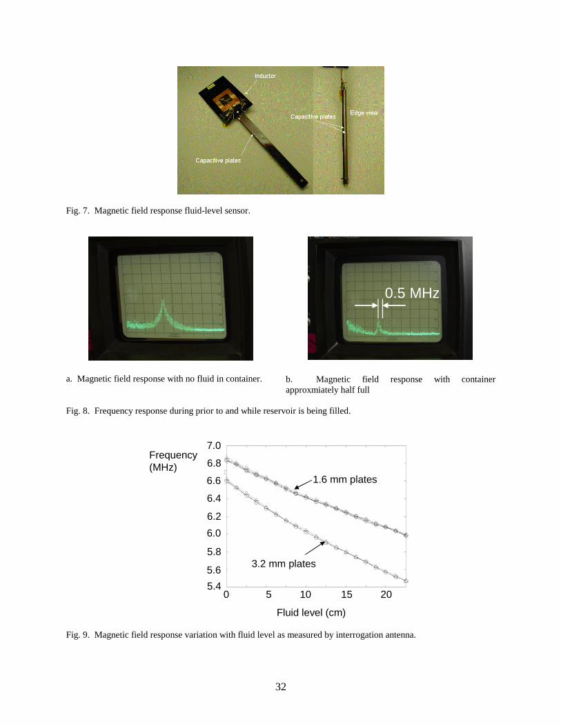
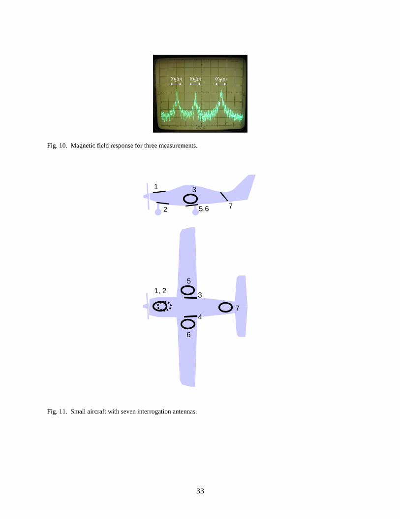
Two Sensor Examples Example 1 - Measurement of Material Phase Transition Figure 5 shows the magnetic field response sensor used to measure material phase transition. The inductor (L) is formed as a square spiral trace of copper. Interdigital electrodes have been used for the capacitor (C). The inductor and the capacitor have been deposited on a thin dielectric film. A single antenna was used to power the sensor and to receive its response. The resonant frequency of the sensor was 5.6 MHz. The sensor was placed in the bottom of a plastic container. Liquid resin was poured into the container and became a dielectric of the capacitor resulting in the sensor resonant frequency changing to 4.8 MHz. As the resin cured, its dielectric constant changed resulting in a changed capacitive value of the L-C ciruit. Figure 6 shows a time history of the magnetic field response resonant frequency during resin curing. As seen in Fig. 6, the response frequency no longer changed after 100 minutes when the curing was complete. The embodiment in Fig. 5 can also be used for strain measurements. When the sensor is fixed to a surface, the distance, d, between electrodes will change when the surface is strained. As the separation changes, the capacitance and thus the resonant frequency of the circuit changes. Example 2 - Measurement of Fluid-Level A magnetic field response fluid-level sensor is shown in Fig. 7. The sensor consists of two capacitive plates electrically coupled to an inductor. The capacitor was placed in a cylindrical container while the inductor remained outside the container. The container was filled with hydraulic fluid. As the fluid filled the void between the plates, the dielectric exposure increased proportional to fluid immersion and thus changed the sensor’s resonant frequency. The magnetic response is shown in Fig. 8 for an empty container (Fig. 8a) and when the container is half full (Fig. 8b). Frequency measurements for two 23 cm fluid-level sensors of different widths are shown in Fig. 9. As the levels increased, the frequencies decreased. Fluid level was increased using 13 mm increments. A fluid-level of 23 cm resulted in frequency reductions of over 1.1 MHz (3.2 mm plate width) and 0.8 MHz (1.6 mm plate width) from that of the empty container. The sensor embodiment in Fig. 5 can also be used for measuring the fluid levels of nonviscous fluids. The electric field of the interdigital electrodes arcs from one positive electrode to its neighboring negative electrode. Most of the interdigital electrode’s electric field is near the plane of the electrodes whereas the electric field of the capacitive plates is perpendicular to the plates. The interdigital electrode’s electric field has proportionally more exposure to the viscous fluid film residue (and more dielectric exposure) than that of the plates. The capacitive plates are necessary when viscous fluids are used because any residual film has a negligible effect on measurements. The amount of plate separation is designed to eliminate capillary effects. When nonviscous fluids are used (e.g., water, gasoline, alcohol), the interdigital electrodes do not require the volume necessary for plates since they can be placed on thin-film dielectrics or directly deposited to a surface. The interdigital electrodes are easier to fabricate and mount. Figure 10 shows the response from multiple sensors. In this example, a broadband of magnetic energy (1-10 MHz) excited the sensors. Each sensor has a predetermined frequency range, Fig.

9

3, which is correlated to its measurement range. The resonant peaks shown are for a fluid-level measurement, ω1(p), position measurement, ω2(p), and proximity measurement, ω3(p). The range of frequencies (i.e., partition) for each measurement is annotated (arrows). Two examples of magnetic field response sensors have been presented in this section. The next section discusses methods of developing sensors to accommodate other classes of measurement. Methods of Developing Magnetic Field Response Sensors This section presents methods of using components of the magnetic field response sensors for measurements of physical properties or to provide a means of numerical encoding. Variations of capacitive plate geometry, interdigital electrode geometry, capacitor dielectric, inductance, inductor permeability, and the use of piezoelectric material in lieu of capacitors are discussed in the following six subsections. Capacitive Plate Geometry Variation When two opposing plates are used for capacitors, the capacitance is dependent upon the distance between the plates and the area overlap of the plates. As the separation between capacitive plates decreases, capacitance increases and sensor resonant frequency decreases. When used to form a sensor, inductance is fixed. Sensors that use plate separation can be used for the following measurements: - Proximity sensing - Each plate is attached to a separate surface. When near each other (<3

mm), change in surface separation changes resonant frequency.

- Pressure9,10,15

- Plates are elastic with fixed boundaries. Surface deformation due to external pressure alters separation distance between plates.

- Strain - Any strain will alter the distance between the plates and therefore change sensor resonant frequency. Each plate can be attached separately and perpendicular to a surface, oSr, each plate can be embedded in a medium with surface of plates perpendicular to direction of strain.

- Compression/tension force – If the plates are attached to or embedded in material of known modulus of elasticity, compression and tension force can be derived by product of strain and material elastic modulus.

The area overlap (effective area) of two opposing plates can also be used to acquire certain measurements when inductance is fixed. As the overlap area between capacitive plates increases, capacitance increases and sensor resonant frequency decreases. As plates move parallel to each other, the effective area changes. The electric field exists only within the area for which the plates overlap. The effective capacitance area can be used to develop sensors for the following measurements:

- Position14

– One plate is fixed and the other plate moves in a single direction with plate surfaces being parallel. The position of one plate along the line of displacement changes relative overlap of plates and thus sensor resonant frequency.

10

- Shear force - A dielectric of known shear modulus is sandwiched between the plates and attached to interior surfaces of plates. Shear force is proportional to the relative displacement of the plates.

- Torsion torque – Rectangular plates are used. A dielectric of known torsion modulus is sandwiched between the plates and attached to interior surfaces of plates. One plate is fixed and the other plate is rotated about its normal. The torsion torque is inversely proportional to relative capacitive area. Higher sensitivity is achieved by using rectangular plates of high aspect ratio.

Relative plate orientation can be used to make sensors for angular measurements. Both plates must have a common axis of rotation and inductance is fixed. When the plates rotate relative to each other, the resonance frequency changes. Interdigital Electrode Geometry Variation Interdigital electrodes can be used as a capacitor. Geometric variations to interdigital electrodes, Fig. 5, can also be correlated to changes in physical states. The interdigital electrode is affixed to a surface and its deformation is compliant with any surface deformation. In-plane strain changes the distance, d, between neighboring electrodes resulting in a change to capacitance and thus sensor resonant frequency. Discrete changes to the number of active electrode pairs can be used to develop a magnetic field response equivalent of numerals. A numeric base is selected and the number of electrode pairs is that of the base. The use of interdigital electrodes allows flexibility in selecting base (e.g., binary, octal, decimal, hexadecimal, etc.) for numerical coding. For example (using base 10), a single number can be developed as a single inductor in parallel with 10 electrode pairs. Each L-C circuit is a single digit. When more than one digit is needed, similar circuits can be used with different inductance levels used to distinguish the digits. The inductance decreases with increased exponent of digit. A numeral is determined by the number of active electrode pairs (i.e., in the nonopened portion of the circuit). The number that the circuit represents is the number of active electrode pairs subtracted from the numeral base. For example, the number 6 is derived by terminating 4 electrode pairs from the initial 10 pairs of electrodes. Terminating a number of active electrode pairs equal to that of the desired number’s complement results in resonant frequency being scaled to the number.

11

Capacitor Dielectric Variation Dielectric changes to the capacitor can be used for a variety of measurements. Dielectric immersion (e.g., into a fluid or solid particles like sand) changes the sensor resonant inversely to

dielectric immersion.8,16

Resonant frequency changes continuously when capacitive plates are immersed in a dielectric medium. The resonance change is discrete when interdigital electrodes are used. The changes are reversible. Similarly, some environment exposures are reversible. Vapor or gas exposed to electrodes or capacitive plates becomes a sensor dielectric. The change

in resonant frequency depends upon the chemical and amount of exposure.11,12

When the capacitors are exposed to or immersed in a dielectric undergoing a material phase transition, the phase transition produces a resonant frequency change (Figs. 5 and 6). The resonant change is permanent if the material phase transition is permanent (e.g., resin cure) or non-permanent if the phase transition can be reversed (e.g., water freezing then melting). A dielectric can be designed as a reactant to a chemical reaction. When exposed to another reactant capable of producing a chemical reaction, the chemical reaction alters the dielectric, thus changing the response frequency. Examples are a palladium dielectric exposed to hydrogen gas (a means of developing a hydrogen detector) or a silicon dielectric exposed to oxygen (a means of developing an oxygen detector). Each example permanently alters the dielectric properties. Inductive Variation When an inductor is placed in proximity to a conductive material, its inductance decreases as the inductor is brought closer to the material. When a flat inductor (Figs. 5 and 6) is used, the proximity to a flat conductive surface can be measured. The rate that inductance changes with position from conductive material is dependent upon the skin depth of the material. Inductance changes as distance to a conductive surface varies due to eddy currents being produced in the conductive surface. As an inductor is moved closer to surface, the magnetic field response amplitude decreases and frequency increases. The following sensors can be developed from the above-mentioned phenomena: - Bond separation – A conductive surface is placed on one side of a surface bond and a flat

magnetic field response sensor (Figs. 5 and 6) on the other side of a bond such that the conductive surface and the sensor are in proximity to each other. If the bond is broken, the inductance will change. An example would be that for steel-belted tires. If a sensor is placed on the inside wall of the tire, any separation of the steel belts from the rubber would result in an inductance change.

- Strain - Method is similar to that used when capacitive plates are used. An inductor is substituted for one capacitive plate and a conductive surface is used instead of the other plate.

- Tension/compression force – Method is similar to that used when capacitive plates are used. An inductor is substituted for one capacitive plate and a conductive surface is used instead of the other plate.

12

When distance separating inductor and conductive surface is fixed, the amount of inductance is proportional to the area overlap of inductor and conductive surface. In a manner similar to capacitive plate overlap variation, one surface has a conductive material and the other has the inductor. Applications are measurements of position, displacement, shear load, and torsion load. Relative plate orientation can be measured similar to the method used for capacitive plates. The orientation between the antenna and the inductor can be inferred using Eqs. (3) and (5) of Appendix A and therefore provides a means of determining sensor orientation when antenna-inductor separation is fixed. Inductor distance from receiving and transmitting antenna(s) can be used for position and displacement measurements. When capacitance and inductance are fixed, amplitude of response is dependent upon inductor distance from receiving antenna and transmitting antenna. Both antennas must have fixed position and orientation. Response frequency will not vary but response amplitude will vary as inductor’s position relative to antenna(s) changes. Applications are displacement and displacement rate measurements such as tire rotation, motion of a linkage, etc. In a manner similar to the number of active interdigital electrode pairs, the relative number of inductors in series or the effective length of an inductor can be used to produce the magnetic field equivalent of a specific number. Inductor Permeability Variation Changes to the material surrounding an inductor for which a magnetic field is being produced change the permeability of the material and thus the inductance of the sensor. In manners similar to those resulting in changes to capacitor dielectric, the same effects can be used to change an inductor’s permeability, therefore providing the means of developing sensors. Use of Piezoelectric Material in Lieu of Capacitors Piezoelectric material can be used as capacitive component of the sensor. Piezoelectric materials (e.g., piezo-ceramics such as lead zirconate-titanate (PZT), or piezo-polymers such as polyvinyldinofloruride (PVDF)) have electrical properties similar to capacitors.17 These materials develop electric polarization when force is applied along certain directions. The magnitude of polarization is proportional to the force (within certain limits). The capacitance varies as the polarization varies which is sufficient for measuring resulting strain from material deformation. Deformation can be due to either mechanical or thermal loading (pyroelectric effect). These materials can be used in lieu of capacitors for strain and temperature measurements.17

13

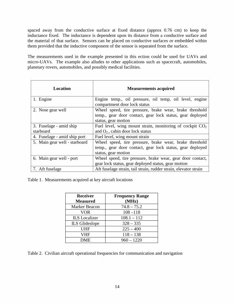
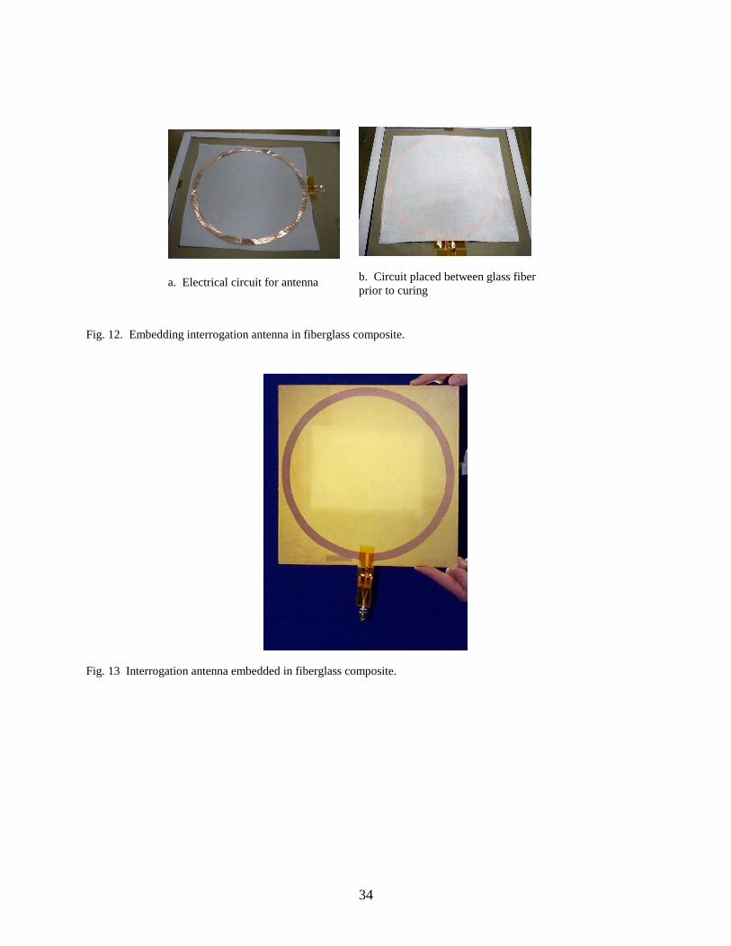
Example of Implementating Measurement Method This section presents an example of implementing the measurement acquisition system on a small aircraft. Figure 11 shows 7 antennas locations on the aircraft where many critical measurements are required. Although 7 antennae are shown, it may be possible to combine them. Measurements for each antenna are listed in Table 1. Two measurement configurations were used to quantify effective range for measurement acquisition. In the first configuration, a switching antenna (30.5 cm loop) was used with a transmission power level of 0.1 W. An inductor with a 12.7 cm x 12.7 cm square spiral with 1.9 cm trace coupled to a 504-pF capacitor achieved a –60 dB response at 63.5 distance from the antenna. The inductor with the 7.62 cm x 7.62 cm. square spiral with 0.63 cm. trace coupled with a 826-pF capacitor achieved a –60 dB response at 55.9 cm distance from antenna. In the second measurement configuration, a transmission antenna (45.7 cm outer diameter and 1.3 cm trace) and receiving antenna (wire loop 61 cm using 12 gauge copper wire) are used. They are positioned 3.3 m apart. The antennas are operated such that when the transmission antenna is powered on to excite the sensors, the receiving antenna is off. The transmission antenna used 1.5 W of power. When the transmission antenna is switched off, the receiving antenna is powered on allowing it to receive the sensor response. In this configuration, the sensors could be interrogated anywhere in a volume approximated by a cylinder whose longitudinal axis runs between the antenna centers and with diameter approximately 1.23 m. The length of the cylinder was the separation distance between the antennas. When the antennas were separated by 2.7 m, the same sensors could be interrogated using 1.0 W of power. The distance measurements demonstrate that the measurement system antennas can be placed at key locations on the plane. Table 2 lists communication and navigation operational frequencies for civilian aircraft. To alleviate electromagnetic interference with communication and navigation frequencies, the sensors’ frequencies should be less than 74.8 MHz (marker beacon) or greater than 1220 MHz (Distance Measuring Equipment (DME)). Table 1 lists 39 types of measurements. Some types of measurements could be done by numerous sensors at different locations (e.g., multiple strain sensors). The 7 antennas would interrogate a minimum of 39 measurements. Using traditional data acquisition methods would require 39 data channels. If strain sensors that use interdigital capacitors and spiral inductors are directly deposited to the wing, tail, and fuselage, these sensors cannot only provide strain measurements but slight cracks (at their placement) would alter either their capacitance or inductance providing crack detection capabilities. When the aircraft are constructed using nonconductive material such as fiberglass, the antennas can be embedded or deposited onto the fiberglass lamination. Figure 12 shows an antenna prior to being embedded into a fiberglass laminate. The finished laminate with the antenna is shown in Fig. 13. Similarly, sensors can also be embedded into the nonconductive composites. The sensors and inductors can also be placed on completed nonconductive composites. Conductive composites using graphite fibers or metallic surfaces require the inductive component to be

14

spaced away from the conductive surface at fixed distance (approx 0.76 cm) to keep the inductance fixed. The inductance is dependent upon its distance from a conductive surface and the material of that surface. Sensors can be placed on conductive surfaces or embedded within them provided that the inductive component of the sensor is separated from the surface. The measurements used in the example presented in this ection could be used for UAVs and micro-UAVs. The example also alludes to other applications such as spacecraft, automobiles, planetary rovers, automobiles, and possibly medical facilities.

Location

Measurements acquired

1. Engine Engine temp., oil pressure, oil temp, oil level, engine compartment door lock status

2. Nose gear well Wheel speed, tire pressure, brake wear, brake threshold temp., gear door contact, gear lock status, gear deployed status, gear motion

3. Fuselage - amid ship starboard

Fuel level, wing mount strain, monitoring of cockpit CO2

and O2 , cabin door lock status 4. Fuselage - amid ship port Fuel level, wing mount strain 5. Main gear well - starboard Wheel speed, tire pressure, brake wear, brake threshold

temp., gear door contact, gear lock status, gear deployed status, gear motion

6. Main gear well - port Wheel speed, tire pressure, brake wear, gear door contact, gear lock status, gear deployed status, gear motion

7. Aft fuselage Aft fuselage strain, tail strain, rudder strain, elevator strain Table 1. Measurements acquired at key aircraft locations

Receiver Measured

Frequency Range (MHz)

Marker Beacon 74.8 – 75.2 VOR 108 –118

ILS Localizer 108.1 – 112 ILS Glideslope 328 – 335

UHF 225 – 400 VHF 118 – 138 DME 960 – 1220

Table 2. Civilian aircraft operational frequencies for communication and navigation

15

Concluding Remarks A measurement acquisition method using magnetic field response sensors has been presented. The magnetic field response sensor serves as a means of acquiring power via Faraday induction, a sensor, and a means of transmitting the measurement via the magnetic field created by the inductor. The acquisition method was developed to acquire measurements from any magnetic field response sensor and to increase the distance between an interrogation antenna and the sensors. The method facilitates multiple measurements having different dynamic characteristics. Dynamic variations of response frequency, amplitude, and bandwidth can be analyzed with the method. To increase the capability of the method, a technique was presented that allows for variations in sensor resistance to be measured with only knowing the amplitude at resonance and at a set frequency prior to that. The system also allows for autonomous sensor interrogation and analysis of collected response. The method greatly reduces the difficulty of implementing a measurement system. Sensor physical connection to a power source (i.e., lead wires) and data acquisition equipment are not needed. Multiple sensors can be interrogated using the single data acquisition channel used for the antenna. Key components (inductors, antennas, some capacitor types) of the method can be developed as metallic foils, thin films, or directly deposited on a surface during manufacturing. No line-of-sight is required between antenna and sensor. The entire sensor can be embedded in nonconductive material. For conducting material, the capacitor can be embedded and the inductor can be placed away from the surface of the conductive material. No specific orientation of sensor with to respect the antenna used to excite the sensor is required except that they cannot be 90 deg to each other. Because no wiring is required, it is easy to add new measurements. Methods to develop magnetic field response sensors were presented. Various components of the sensors can be designed to change correspondingly to the physical state for which the sensor is measuring. Sensors described from the methods included the means to measure shear force, torsion force, strain, pressure, environmental, material phase transition, dielectric immersion (e.g., fluid level), displacement, and proximity. Also discussed were methods of developing a numeric encoding system. Two examples of sensors were presented: fluid-level sensor and material phase transition sensor. The material phase transition sensor was placed in a liquid resin. The resonant frequency of the sensor was measured until there was no change in it indicating a cured resin. Fluid-level measurements were also presented. A fluid level of 23 cm resulted in a frequency reduction of over 1 MHz from that of the empty container. An example of implementing the system on an aircraft demonstrated the advantages of the system. Multiple measurements were consolidated to a few data channels (one channel per antenna). Many of the sensors were easy to place on the aircraft during manufacturing or during replacement of parts. Use of the system is applicable to all aerospace systems. The elimination of wires and integrated circuits physically connected to a sensor allows for use in harsh chemical, thermal, or radiative environments. Mathematical models of the antenna magnetic field and the sensor magnetic field illustrated how key parameters influence sensor interrogation. The model also highlighted parameters such as

16

antenna and inductor resistance which could be reduced by effective design of such components. Methods to increase antenna and inductor effectiveness were also presented as techniques to increase the distance between an interrogation antenna and a sensor. The distance at which the magnetic inductor response can be received is proportional to how strong the magnetic field created in the inductor is. The magnetic field strength is dependent upon the current in the sensor. Therefore, interrogation distance is also dependent upon the energy efficientcy of the sensor circuit. The higher the energy efficiency, the more current that is created for the same level of power used by the interrogating antenna(s).

17

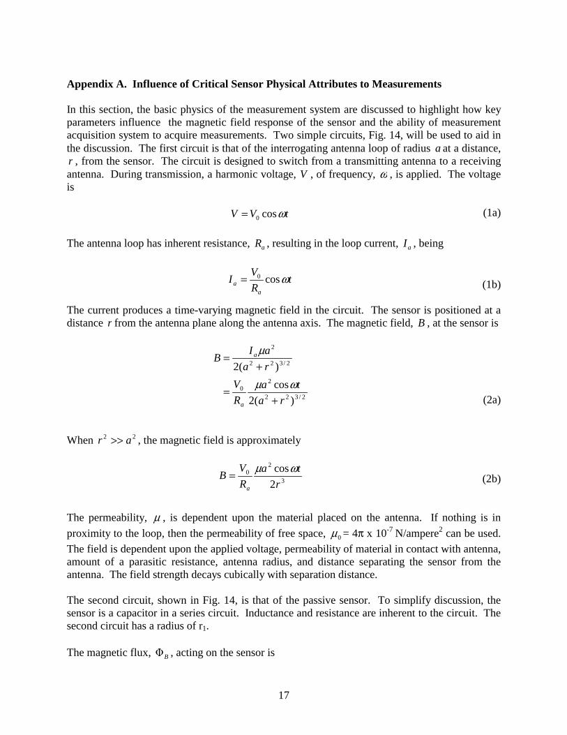
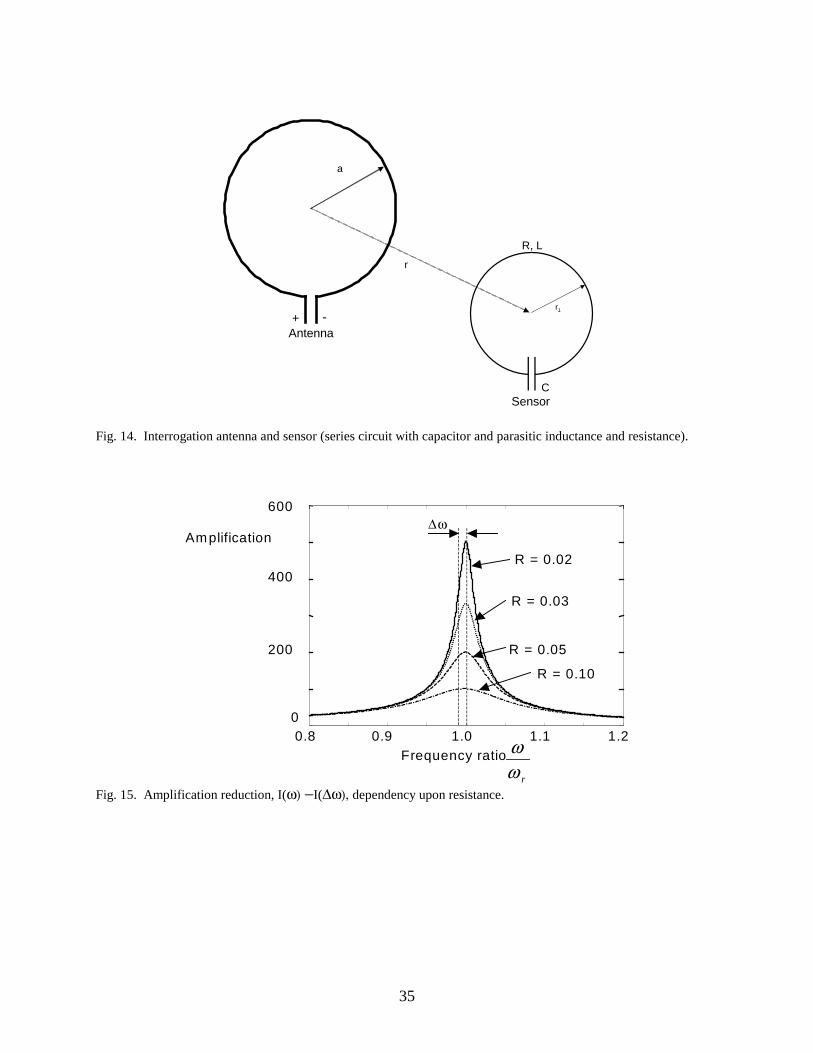
Appendix A. Influence of Critical Sensor Physical Attributes to Measurements In this section, the basic physics of the measurement system are discussed to highlight how key parameters influence the magnetic field response of the sensor and the ability of measurement acquisition system to acquire measurements. Two simple circuits, Fig. 14, will be used to aid in the discussion. The first circuit is that of the interrogating antenna loop of radius a at a distance, r , from the sensor. The circuit is designed to switch from a transmitting antenna to a receiving antenna. During transmission, a harmonic voltage, V , of frequency, ω , is applied. The voltage is

tVV ωcos0= (1a)

The antenna loop has inherent resistance, aR , resulting in the loop current, aI , being

tR

VI

aa ωcos0=

(1b)

The current produces a time-varying magnetic field in the circuit. The sensor is positioned at a distance r from the antenna plane along the antenna axis. The magnetic field, B , at the sensor is

2/322

20

2/322

2

)(2

cos

)(2

ra

ta

R

V

ra

aIB

a

a

+=

+=

ωµ

µ

(2a)

When 22 ar >> , the magnetic field is approximately

3

20

2

cos

r

ta

R

VB

a

ωµ=

(2b)

The permeability, µ , is dependent upon the material placed on the antenna. If nothing is in

proximity to the loop, then the permeability of free space, 0µ = 4π x 10-7 N/ampere2 can be used.

The field is dependent upon the applied voltage, permeability of material in contact with antenna, amount of a parasitic resistance, antenna radius, and distance separating the sensor from the antenna. The field strength decays cubically with separation distance. The second circuit, shown in Fig. 14, is that of the passive sensor. To simplify discussion, the sensor is a capacitor in a series circuit. Inductance and resistance are inherent to the circuit. The second circuit has a radius of r1. The magnetic flux, BΦ , acting on the sensor is

18

SB dB ⋅= ∫Φ (3)

Note that B is a vector of flux strength and direction while S is a vector proportional to the sensor surface area in the normal direction. Maximum flux occurs when the flux and the sensor normal are parallel. Measurements can be acquired as long as these vectors are not perpendicular. When sensor normal and flux are parallel, the flux is

3

22

10

2

cosΦ

r

tar

R

V

aB

ωµπ=

(4)

In accordance with Faraday’s law of induction, the induced electromotive force, ε , produced in the sensor is equal in magnitude to the rate of change in the flux.

dt

d BΦ−=ε

At the sensor, this quantity is

3

22

10

2

sin

r

tar

R

V

a

ωµωπε =

5)

When the magnetic field of the antenna is harmonic, the resulting electromotive force produced in the sensor is dependent upon flux, the area of sensor, and is proportional to the frequency of the flux. Thus far, we have derived the electromotive force in the sensor. We will now show what factors influence the magnetic field produced by the sensor. The dynamics of the sensor in terms of current produced by the electromotive force is now presented followed by the magnetic field produced by the current, I . The constituent components of the sensor are in series. The differential equation describing the dynamics of current in the sensor is

tIdtC

RIIL ωε sin 1

0∫ =++′

(6a)

with

3

22

10

0 2r

ar

R

V

a

µωπε =

and L , R , and C are the sensor’s inherent inductance, inherent resistance, and capacitance.

19

Equation (6a) is differentiated to eliminate the integral resulting in

tIC

IRIL ωωε cos1

0=+′+′′ (6b)

The solution to (6b) is

−+

−−+−

+= tRtS

eSReRS

RStI

tt

TX ωωλλ

λωωλε λλ

sincos)(

)()(

)()(

21

1222

021

(7)

with

)1

(C

LSω

ω −=

C

LR

LL

R 4

2

1

22

1 −+−=λ

C

LR

LL

R 4

2

1

22

2 −−−=λ

The subscript, TX , has been added to the current to denote the antenna is transmitting. The term, S , is called the reactance.

The sensor current when the antenna is transmitting is given by Eq. (7). The steady state response of the sensor’s current while the antenna is transmitting Eq. (7) is

)sin()( 0 θω ±= tItI p (8)

where

22

00

RSI

+=

ε

(9)

and

R

S±=θtan

The term 22 RS + is called the impedance.

Eq. (9) has the influence of sensor’s resistance, reactance and electromotive force level on the steady current amplitude, 0I , when the antenna is transmitting. It can be concluded by

examination of Eq. (9); the amplitude is maximized by minimizing resistance and reactance.

20

Resistance is minimized by increasing electrical efficiency of constituent components. Reactance is zero when the antenna broadcast frequency is that of the undamped resonance of the inductive-capacitive circuit which is

LC

1=ω

The time to reach steady state is dominated by the larger of the two roots, 1λ . As can be seen from the root, the decay rate is proportional to resistance and inversely proportional to inductance. After a finite amount of time, t∆ , the interrogation antenna is switched to the receiving mode thus removing the electromotive force from the sensor circuit. The sensor current response is now

01 =+′+′′ IC

IRIL

(10)

The response is overdamped if C

LR

42 > , critically damped if C

LR

42 = , or underdamped if

C

LR

42 < . The overdamped response could occur if a resistive type measurement is added to the

circuit and inductance and capacitance are kept constant. If an operational objective is to have considerable separation distance between the circuit and antenna, then the circuit should only be composed of capacitors and inductors. If possible, the circuit should be designed to reduce inherent resistance. Hence, we will examine the underdamped response. The solution for the underdamped case is

−−+−−=

−−

))(4

1sin())(

4

1cos()(

2

2

2

2)(2 tt

L

R

LCBtt

L

R

LCAetI

ttL

R

RX ∆∆∆

(11)

AtItI TXRX == )()( ∆∆

The subscript, RX , has been added to the sensor current to denote the antenna is receiving. The decay envelop depends on

L

R

2

− . The current value in the sensor, )( tITX ∆ , when the antenna is

switched to a receiving antenna, and current derivative value, )( tITX ∆′ , are the initial conditions used to determine coefficients A and B .

21

In a manner similar to the antenna, the magnetic field produced by the sensor is now

3

21

2

)(

r

rtIB RX

RX

µ= for 21

2 rr >>

(12)

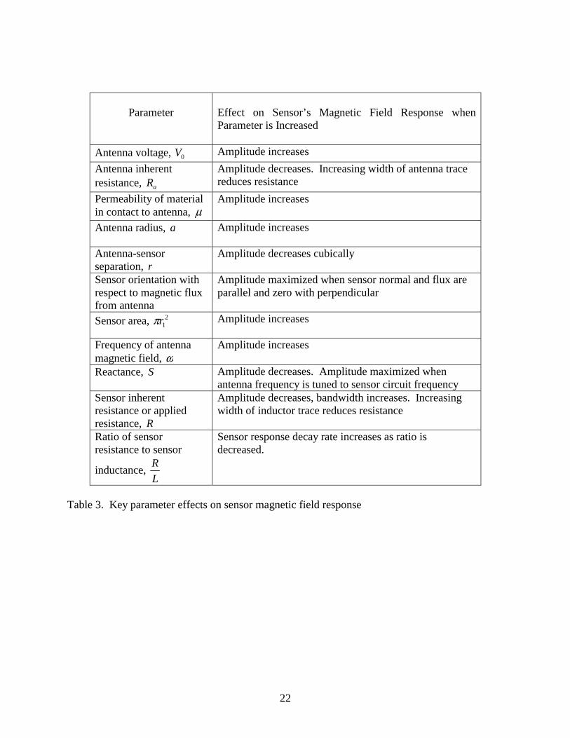
As can be seen by Eq. (12), the magnetic field is dependent upon the sensor current which is dependent upon the electromotive force, reactance, and resistance. During subsequent transmission intervals, the final conditions from the prior mode (e.g., transmission or reception) are the initial conditions for the current mode. Hence, each transmission and reception interval has a closed form solution for current response. Table 3 summarizes the influences of the parameters on sensor magnetic field response.

22

Parameter

Effect on Sensor’s Magnetic Field Response when Parameter is Increased

Antenna voltage, 0V Amplitude increases

Antenna inherent resistance, aR

Amplitude decreases. Increasing width of antenna trace reduces resistance

Permeability of material in contact to antenna, µ

Amplitude increases

Antenna radius, a Amplitude increases

Antenna-sensor separation, r

Amplitude decreases cubically

Sensor orientation with respect to magnetic flux from antenna

Amplitude maximized when sensor normal and flux are parallel and zero with perpendicular

Sensor area, 21rπ Amplitude increases

Frequency of antenna magnetic field, ω

Amplitude increases

Reactance, S Amplitude decreases. Amplitude maximized when antenna frequency is tuned to sensor circuit frequency

Sensor inherent resistance or applied resistance, R

Amplitude decreases, bandwidth increases. Increasing width of inductor trace reduces resistance

Ratio of sensor resistance to sensor

inductance, L

R

Sensor response decay rate increases as ratio is decreased.

Table 3. Key parameter effects on sensor magnetic field response

23

Appendix B. Measuring Sensor Resistive Variations The previous section presented the effect of key parameters on the magnetic field response. This section presents a method whereby resistive variations can be discerned using only two points of the magnetic field response curve. The bandwidth of the response is proportional to the circuit resistance. However, to measure bandwidth one would need to identify the response peak and then measuring the response curve on either side of the peak to ascertain the 3 dB reductions in amplitude. To identify the 3 dB reduction would require measuring all amplitudes for each discrete frequency until the reduction amplitudes are identified. Another method to identify resistance is to examine how much the amplitude is reduced from the peak at a fixed frequency, ω∆ , separation from the resonant frequency, rω . Fig. 15 illustrates response curves for four resistive values. As can be seen from the figure, the difference in amplitude between the peak response, 0I , and the amplitude at a fixed frequency away, )( *ωI , is inversely proportional

to resistance. The magnetic field of the sensor is proportional to its current. The current at the *ω is

22*

*

0*

)1

(

)(

RC

L

I

+−=

ωω

εω

(13)

where

ω∆ωω −= r*

The amplitude reduction is

)11

()()(22*

0*

RSRII r

+−=− εωω

(14)

where

CLS

*** 1

ωω −=

Because

RRS >+ 22*

24

22*

11

RSR +>

The above expression is monotonic with respect to R for fixed *S . Therefore,

))()(( *ωω IIfR r −= (15)

The expression is not closed form but it does indicate that resistive measurements can be derived from the difference in amplitudes, )()( *ωω II r − . Once amplitude reduction variation with

resistance, ))()(( *ωω IIfR r −= , has been characterized, this method requires only two amplitude measurements to determine resistance as compared with the multiple measurements required to determine 3 dB reduction.

25

References 1Woodard, S. E., Coffey, N. C., Gonzalez, G. A., Taylor, B. D., Brett, R. R., Woodman, K. L., Weathered, B. W. and Rollins, C. H., “Development and Flight Testing of an Adaptable Vehicle Health-Monitoring Architecture,” Journal of Aircraft, Vol. 40, No. 5, September-October 2003. Also documented as NASA Technical Memorandum 2003-212139, January 2003. 2Carreau, Mark, “Wire Damage Discovered in All Four Space Shuttles,” Houston Chronicle, Aug. 16, 1999. 3Ray, Justin, “Wiring Review Delays Delta 2 Launch of Air Force Satellite,” Spaceflight Now, July 25, 2002. 4National Transportation Safety Board, “Aircraft Accident Report: In-flight Break-up Over the Atlantic Ocean , Trans World Airlines Flight 800, Boeing 747-131, N93119 Near East Moriches, New York, July 17, 1996,” NTSB/AA-00/03, DCA96MA070, PB2000-910403, Notation 6788G, Aug. 23, 2000. 5Transportation Safety Board of Canada, “Aviation Investigative Report: In-Flight Fire Leading to Collision with Water, Swissair Transport Limited, McDonnel Douglas MD-11 HB-IWF, Peggy’s Cover, Nova Scotia 5nm SW, 2 Septermber 1998,” Report Number A98H0003. 6Halliday, D., and Resnick, R. “Physics Part Two,” John Wiley and Sons, New York, NY, 1978, pp. 650-665 and 770-888. 7Lorrain, P., and Corson, D., “Electromagnetic Fields and Waves,” W. H. Freeman and Company, 1970, San Francisco, CA, pp. 91-128 and 292-373. 8Konchin, B., Slavik, I., and Coery, R. W., “Fluid Sensing System,” U. S. Patent 6, 335, 690, Jan. 2002. 9Fonseca, M. A., English, J. M., Arx, M. V., and Allen, M. G., “High Temperature Characterization of Ceramic Pressure Sensors,” Proceeding of 1999 IEEE MEMS Workshop, pp. 146-149. 10Allen, M. A., and English, J. M., “System and Method for the Wireless Sensing of Physical Properties,” U. S. Patent 6, 11,520, Aug. 2000. 11Ong, K. C., Grimes, C. A., Robbins, C. L., and Singh, R. S., “Design and Application of a Wireless, Passive, Resonant-Circuit Environmental Sensor,” Sensors and Actuators, A 93, 2001, pp. 33-43.

26

12Ong, K. C., Zeng, K., and Grimes, C. A., “A Wireless, Passive Carbon Nanotube-Based Gas Sensor,” IEEE Sensors Journal, Vol. 2, No. 2, April 2002, pp. 82-88. 13Butler, J. C., Vigliotti, A. J., Verdi, F. W., and Walsh, S. M., “Wireless, Passive, Resonant-Circuit, Inductively Coupled, Inductive Strain Sensor,” Sensors and Actuators, A 102, 2002, pp. 61-66. 14Bullara, L. A., “Implantable Pressure Transducer,” U. S. Patent 4, 127, 110, Nov. 1978. 15Pinto, G. A. and Briefer, D. K., “Capacitive Pressure Sensor Having Encapsulated Resonating Components,” U. S. Patent 6,532,834, March 2003. 16Woodard, S. E., Taylor, B. D., Shams, Q. A., and Fox, R. L., “L-C Measurement Acquisition Method for Aerospace Systems,” Proceedings of the 2003 AIAA Aviation Technology, Intergration and Operations Technical Forum, AIAA Paper No. 2003-6842, Denver,CO, November 17-19, 2003. 17T. Ikeda, “Fundamentals of Piezoelectricity,” Oxford: Oxford University Press, 1990.

27

Discern resonant frequency of response

Antenna

Transmit magnetic field at a single frequency to electrically excite sensor

Acquire time history of response radiated from sensor

Switch to receiving antenna

Sensors

Cn(p)

Ln

C1(p)

L1

…

Magnetic Harmonic,ω1

Magnetic Harmonic,ωn

Fig. 1. Schematic of magnetic field response measurement acquisition method.

28

Switch to transmission mode. Increment frequency. Transmit magnetic field.

Compare amplitude with previous two amplitudes.

Interrogate next sensor

Transmit magnetic field at a single frequency. Switch to reception mode.

Rectify response received from sensor. Store amplitude and frequency.

NO

YES

Ai < Ai-1 and Ai-1 > Ai-2

Rectify response received from sensor. Store amplitude, Ai, and frequency, ωi.

Fig. 2. Magnetic field response acquisition method interrogation logic.

29

Sensor 1Range

Sensor 2Range

Sensor 3Range

Sensor n

∆ω1 ∆ω2 ∆ω3= variable

ω1L ω1U ω2L ω2U ω3L ω3U ωnFirst Sweep

Sensor n

ω1L ω1U ω2L ω2U ω3L ω3U ωn

ω1L ω1U ω2L ω2U ω3L ω3U ωn

Third SweepFrequency

…ω1(p) ω2(p)

ω1(p)

Second sweep

ω3(p) An(p)

Sensor 1 range

An(p)

An(p)ω1(p) ω2(p) ω3(p)

Fig. 3. Magnetic field response sensor measurement bands and resolution during successive frequency sweeps.

30

0.0 0.2 0.4 0.6 0.8 1.0 1.2 1.4 1.6 1.8 2.0

Frequency (Ratio, )

Low resistance

High Resistance

ResponseAmplification

∆ω

Ai

Ai-1 Ai+1

rωω

Fig. 4. Magnetic field response resulting from electromotive force produced via Faraday induction.

31

Capacitor

Inductor

d

a. Schematic of sensor

Inductor

Capacitor

b. Fabricated sensor

Fig. 5. A magnetic field response sensor fabricated onto dielectric film. The inductor (L) is formed as a spiral of copper. Interdigital electrodes have been used for the capacitor (C ).

4.6

4.7

4.8

4.9

5

5.1

0 20 40 60 80 100 120Time (min)

Frequency(MHz)

Fig. 6. Frequency variation during resin curing.

32

Fig. 7. Magnetic field response fluid-level sensor.

a. Magnetic field response with no fluid in container.

0.5 MHz0.5 MHz0.5 MHz0.5 MHz

b. Magnetic field response with container approxmiately half full

Fig. 8. Frequency response during prior to and while reservoir is being filled.

0 5 10 15 20

7.0

6.8

6.6

6.4

6.2

6.0

5.8

5.6

5.4

Fluid level (cm)

Frequency(MHz)

5606, 1/8 in plates

1.6 mm plates

3.2 mm plates

Fig. 9. Magnetic field response variation with fluid level as measured by interrogation antenna.

33

ω1(p) ω2(p) ω3(p)ω1(p) ω2(p) ω3(p)

Fig. 10. Magnetic field response for three measurements.

1

1, 2

2

3

5,6

3

4

5

6

7

7

Fig. 11. Small aircraft with seven interrogation antennas.

34

a. Electrical circuit for antenna

b. Circuit placed between glass fiber prior to curing

Fig. 12. Embedding interrogation antenna in fiberglass composite.

Fig. 13 Interrogation antenna embedded in fiberglass composite.

35

R, L

C

r1

a

r

Antenna

Sensor

-+

Fig. 14. Interrogation antenna and sensor (series circuit with capacitor and parasitic inductance and resistance).

0.8 0.9 1.0 1.1 1.20

R = 0.10

R = 0.05

R = 0.03

600

400

200

Amplification

R = 0.02

∆ω

Frequency ratio

rωω

Fig. 15. Amplification reduction, I(ω) −I(∆ω), dependency upon resistance.

REPORT DOCUMENTATION PAGE Form ApprovedOMB No. 0704-0188

2. REPORT TYPE

Technical Memorandum 4. TITLE AND SUBTITLE

Magnetic Field Response Measurement Acquisition System5a. CONTRACT NUMBER

6. AUTHOR(S)

Woodard, Stanley E.; Taylor, Bryant D.; Shams, Qamar A.; andFox, Robert L.

7. PERFORMING ORGANIZATION NAME(S) AND ADDRESS(ES)

NASA Langley Research CenterHampton, VA 23681-2199

9. SPONSORING/MONITORING AGENCY NAME(S) AND ADDRESS(ES)

National Aeronautics and Space AdministrationWashington, DC 20546-0001

8. PERFORMING ORGANIZATION REPORT NUMBER

L-19074

10. SPONSOR/MONITOR'S ACRONYM(S)

NASA

13. SUPPLEMENTARY NOTESWoodard, Shams and Fox: Langley Research Center; Taylor: Swales AerospaceAn electronic version can be found at http://ntrs.nasa.gov

12. DISTRIBUTION/AVAILABILITY STATEMENTUnclassified - UnlimitedSubject Category 39Availability: NASA CASI (301) 621-0390

19a. NAME OF RESPONSIBLE PERSON

STI Help Desk (email: help@sti.nasa.gov)

14. ABSTRACT

A measurement acquisition method that alleviates many shortcomings of traditional measurement systems is presented in this paper. The shortcomings are a finite number of measurement channels, weight penalty associated with measurements, electrical arcing, wire degradations due to wear or chemical decay and the logistics needed to add new sensors. The key to this method is the use of sensors designed as passive inductor-capacitor circuits that produce magnetic field responses. The response attributes correspond to states of physical properties for which the sensors measure. A radio frequency antenna produces a time-varying magnetic field used to power the sensor and receive the magnetic field response of the sensor. An interrogation system for discerning changes in the sensor response is presented herein. Multiple sensors can be interrogated using this method. The method eliminates the need for a data acquisition channel dedicated to each sensor. Methods of developing magnetic field response sensors and the influence of key parameters on measurement acquisition are discussed.

15. SUBJECT TERMS

Magnetic field response sensor; L-C sensor; Wireless; Health and usage monitoring; Measurement acquisition

18. NUMBER OF PAGES

40

19b. TELEPHONE NUMBER (Include area code)

(301) 621-0390

a. REPORT

U

c. THIS PAGE

U

b. ABSTRACT

U

17. LIMITATION OF ABSTRACT

UU

Prescribed by ANSI Std. Z39.18Standard Form 298 (Rev. 8-98)

3. DATES COVERED (From - To)

5b. GRANT NUMBER

5c. PROGRAM ELEMENT NUMBER

5d. PROJECT NUMBER

5e. TASK NUMBER

5f. WORK UNIT NUMBER

23-762-65-AT

11. SPONSOR/MONITOR'S REPORT NUMBER(S)

NASA/TM-2005-213518

16. SECURITY CLASSIFICATION OF:

The public reporting burden for this collection of information is estimated to average 1 hour per response, including the time for reviewing instructions, searching existing data sources, gathering and maintaining the data needed, and completing and reviewing the collection of information. Send comments regarding this burden estimate or any other aspect of this collection of information, including suggestions for reducing this burden, to Department of Defense, Washington Headquarters Services, Directorate for Information Operations and Reports (0704-0188), 1215 Jefferson Davis Highway, Suite 1204, Arlington, VA 22202-4302. Respondents should be aware that notwithstanding any other provision of law, no person shall be subject to any penalty for failing to comply with a collection of information if it does not display a currently valid OMB control number.PLEASE DO NOT RETURN YOUR FORM TO THE ABOVE ADDRESS.

1. REPORT DATE (DD-MM-YYYY)

02 - 200501-