magnetic tweezers: micromanipulation and force measurement ... · magnetic tweezers:...

Magnetic Tweezers: Micromanipulation and Force Measurement at theMolecular Level

Charlie Gosse and Vincent CroquetteLaboratoire de Physique Statistique, Ecole Normale Superieure, Unite de Recherche 8550 associee au Centre National de la RechercheScientifique et aux Universites Paris VI et VII, 75231 Paris, France

ABSTRACT Cantilevers and optical tweezers are widely used for micromanipulating cells or biomolecules for measuring theirmechanical properties. However, they do not allow easy rotary motion and can sometimes damage the handled material. Wepresent here a system of magnetic tweezers that overcomes those drawbacks while retaining most of the previous dynamometersproperties. Electromagnets are coupled to a microscope-based particle tracking system through a digital feedback loop. Magneticbeads are first trapped in a potential well of stiffness �10�7 N/m. Thus, they can be manipulated in three dimensions at a speedof �10 �m/s and rotated along the optical axis at a frequency of 10 Hz. In addition, our apparatus can work as a dynamometerrelying on either usual calibration against the viscous drag or complete calibration using Brownian fluctuations. By stretching a DNAmolecule between a magnetic particle and a glass surface, we applied and measured vertical forces ranging from 50 fN to 20 pN.Similarly, nearly horizontal forces up to 5 pN were obtained. From those experiments, we conclude that magnetic tweezersrepresent a low-cost and biocompatible setup that could become a suitable alternative to the other available micromanipulators.

LIST OF SYMBOLS

Au (NA�1) the factor between the force and the cur-rent flowing in the coils (Defined in Eq. 2)

� (nondimensional) the proportional feedback factorin the digital model (Defined in Eq. 11)

Bu (�m s�1A�1) the proportional factor between thevelocity of a bead and the associated driving cur-rent (Defined in Eq. 19)

� (nondimensional) the ratio between the integraland the proportional feedback factors (Defined inEq. 17)

Cu (nondimensional) the correction signal in feedbackloop (Defined in Eq. 1)

Cr(f) (nondimensional) the camera filtering correctiondue to its finite integration time (Defined in Eq. 32)

D (�m2s�1) the bead diffusion coefficient (Definedin Eq. 9)

�t (s) the time interval between two video frames (40ms) (Defined in Eq. 12)

�ti (s) the time integration of the video camera (0.97�t) (Defined in Eq. 32)

� (nondimensional) the delay in the feedback loop(Defined in Eq. 11)

�T (s) the integration time of the signal (Defined afterEq. 10)

� (poise) the fluid viscosity (Defined in Eq. 7)Fu (N) the force acting on the bead (Defined in Eq. 2)FL (N) the random Langevin force responsible for the

Brownian motion (Defined in Eq. 7)fc (Hz) the cutoff frequency of the bead attached to

the molecule system, fc � ku/(2��r) (Defined inthe paragraph just after Eq. 8).

fs (Hz) the sampling frequency of the camera (25 Hzhere), fs � 1/�t (Defined in Eq. 31)

fL (Hz) the smallest usable frequency, fL � 1/�T(Defined after Eq. 10)

� (nondimensional) the viscous coefficient of asphere, usually 6� (Defined in Eq. 7)

�x,y (nondimensional) the viscous coefficient of asphere moving parallel to a sidewall (Defined inEq. 30)

�z (nondimensional) the viscous coefficient of asphere moving perpendicularly to a sidewall (De-fined in Eq. 30)

Iu (A) the coil driving current (Defined in Eq. 1)Ium (A) the maximum current set in one direction (De-

fined in Characterization of the Active Tweezers).I0 (A) the minimal value of Iz that lift the magnetic

particle. (Defined in Design of the Apparatus).ku (Nm�1) the stiffness of the tweezers (Defined in

Eq. 2)Ku (�m�1) the integral coefficient in the feedback

loop (Defined in Eq. 1)L0

2(f) (�m2Hz�1) the Langevin force noise density inFourier space (Defined in Eq. 14)

Pu (�m�1) the proportional coefficient in the feed-back loop (Defined in Eq. 1)

r (�m) the bead radius (Defined in Eq. 7)Vu (�m s�1) the bead velocity (Defined in Eq. 9)

INTRODUCTION

During the last ten years, single biomolecule micromanipu-lations have revolutionized the field of biophysics (Bensi-mon, 1996; Bustamante et al., 2000), allowing the biophys-icists 1) to measure the elastic behavior of biopolymers such

Submitted July 6, 2001, and accepted for publication February 21, 2002.

Dr. Gosse’s present address is Institut Curie, Paris, France. E-mail:[email protected].

Address reprint requests to Vincent Croquette, Laboratoire de PhysiqueStatistique, Ecole Normale Superieure, 24 rue Lhomond, 75231 Paris,France. Tel.: �33-1-44-32-34-92; Fax: �33-1-44-32-34-33; E-mail:[email protected].

© 2002 by the Biophysical Society

0006-3495/02/06/3314/16 $2.00

3314 Biophysical Journal Volume 82 June 2002 3314–3329

as actin (Kishino and Yanagida, 1988), titin (Kellermayer etal., 1997 Carrion-Vazquez et al, 1999), or DNA (Cluzel etal., 1996; Strick et al., 1996); 2) to determine the tensilstrength of single ligand/receptor bond (Florin et al., 1994;Merkel et al., 1999); 3) to investigate the micromechanics ofmolecular motors such as kinesin (Block et al., 1990) andmyosin (Ishijima et al., 1991; Finer et al., 1994); 4) tofollow in real time the activity of single proteins such aspolymerases (Yin et al., 1995; Maier et al., 2000; Wuite etal., 2000b); and even 5) to observe single enzymatic cyclesof individual enzymes (Noji et al., 1997; Strick et al., 2000).

Micromanipulation implies monitoring of forces at themolecular scale. In biology, at the single-molecule level, thecharacteristic energy is given by the hydrolysis of ATP (20kT i.e., 80 pN�nm) and the characteristic size by the diameterof a protein (a few nanometers). The resulting forces thatbiophysicists must be able to measure and to produce whilestudying those objects are therefore in the range of hundredsof femtonewtons to tens of piconewtons. In most of thepreviously mentioned studies, the biomolecule is attached toa micromanipulator that works like the spring of a dyna-mometer: after measuring the stiffness of the spring, forcesare deduced from extension measurements. Examples ofmicromanipulators include atomic force microscopy canti-levers (Moy et al., 1994, Carrion-Vazquez et al, 1999), glassfibers (Kishino and Yanagida, 1988; Cluzel et al., 1996),biomembrane force probes (Evans and Ritchie, 1997; Mer-kel et al., 1999), and microbeads held by optical tweezers(Block et al., 1990; Finer et al., 1994; Wuite et al., 2000a).Typical stiffness ranges from 1 N/m for the former to 10�5

N/m for the latter. For measuring biological forces, thetypical extensions that must be detected are consequently ofa few nanometers; a distance also characteristic of thestep-size of molecular motors (Schnitzer and Block, 1997).In this article, we report a new kind of micromanipulator inwhich micrometric particles are monitored and manipulatedin three dimensions (3D) using magnetic field gradients andservo loops. Our apparatus fulfills all the single moleculebiophysics requirements previously mentioned and presentsan alternative to the various existing dynanometers andmanipulators.

The early setups able to manipulate magnetic objects insolution were constructed by biophysicists for the in vivostudy of the viscoelastic properties of the cytoplasm (Crickand Hughes, 1949; Yagi, 1960). More recently, this tech-nique has been applied to the rheology of actin filamentsolutions. After the first experiments by Sackmann andco-workers (Ziemann et al., 1994), in which the motion ofmagnetic particles was confined to a single horizontal axis,Amblard et al. (1996a,b) built a micromanipulator for pre-cise and easily controlled two-dimensional translation androtation of micrometric beads. Independently, magnetic pi-conewton-force transducers have been used to investigatethe elastic behavior of phospholipidic membranes (Hein-rich and Waugh, 1996; Simson et al., 1998). Forces ranging

from hundreds of femtonewtons to nanonewtons were mea-sured, but micromanipulation of the particle was not possi-ble. A somewhat similar apparatus was recently described(Haber and Witz, 2000) with a special care to obtain auniform force on a large spatial domain (1.5 cm). Veryaccurate positioning and force measurements have also beendemonstrated using a macroscopic magnetic particle levi-tated by a single coil (Gauthier-Manuel and Garnier, 1997).Pursuing those works, we report here the design of a mag-netic micromanipulator that could also be used as a new toolfor scientific exploration at the single-biomolecule level.

In its application, our apparatus is very similar to opticaltweezers (Svoboda and Block, 1994; Simmons et al., 1996), itallows displacement of small beads (a few microns in diame-ter) in solution and to use them as handles or picodynamom-eters. The positioning of the particle in 3D is achieved with aprecision of a few nanometers and forces from a few tenths totens of piconewtons are simultaneously measured. In the op-tical tweezers experiment, a particle having a larger refractiveindex than its surrounding medium is trapped by the radiationpressure of a focused laser beam. The intensity profile of thebeam corresponds to a real potential well that traps the bead ina precise location. In our setup, a system of electromagnetscreates field gradients, producing a force on a super-paramag-netic object. Adjusting the current running through the coilsallows us to change the intensity and the direction of this force.Furthermore, by combining, in a feedback loop, this manipu-lator with a video-positioning system, we are able to controlthe 3D position of the particle in real time. Note that, in thiscase, the action of the magnets is global and the particle is, infact, trapped in a virtual potential well by the servo loop.Additionally, we may rotate the object while holding it fixedbecause the direction of the field imposes the angular orienta-tion of the particle magnetic dipole. Finally, after calibration ofthe apparatus, the force acting on the particle can be deter-mined by measuring the currents driving the electromagnets.

The magnetic tweezers described here share most of thefeatures of optical tweezers while offering the advantage ofangular positioning. Moreover, this apparatus does not requirea laser that might photodamage the biomaterial (Liu et al.,1996; Neuman et al., 1999). We believe that it could, in thefuture, meet cell biologists’ needs and allow them precisepositioning of organelles, in vivo microrheological investiga-tions (Crick and Hughes, 1949; Yagi, 1960), and force mea-surements (Wang et al., 1993; Guilford et al., 1995).

DESIGN OF THE APPARATUS

Principle

The apparatus consists of two distinct parts: a 3D position-ing algorithm (discussed later in this section) and a set ofelectromagnets allowing the 3D displacement of the studiedparticle (discussed in the next subsection).

Magnetic Tweezers 3315

Biophysical Journal 82(6) 3314–3329

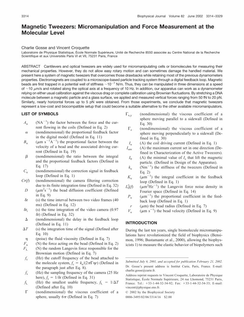
As described in Fig. 1, the cell containing the magneticparticles in solution is held on the stage of an invertedmicroscope. This cell is typically a small capillary tube witha rectangular section (thickness of 300 �m; Vitrocom,Mountains Lakes, NJ). Its top and bottom surfaces are ofgood optical quality. A system of six vertical electromag-nets with their pole pieces arranged in a hexagonal patternis placed just above the capillary tube. Parallel light illumi-nates the sample through a 2-mm-diameter aperture locatedat the center of the hexagon. An xyz translation stage allowsthe accurate positioning of the electromagnets with respectto the optical axis of the objective.

During micromanipulation, a magnetic particle is locatedwith nanometer accuracy by video analysis. The computerprogram determines its position in the three spatial dimen-sions at video rate. Then the digital feedback loop adjuststhe current in each electromagnet to cancel the differencebetween the desired and the observed positions of this bead.The six-fold symmetry of the electromagnets allows rota-tion of the direction of the magnetic field and hence of themagnetic particle itself. The force applied to the bead can bedirectly evaluated by Brownian motion analysis (Strick etal., 1996; Allemand, 1997). This method allows the detec-tion of forces ranging from tens of femtonewtons to tens ofpiconewtons. Alternatively, the force can be read from thecurrents driving the coils. This requires previous force cal-ibration against the viscous drag or against the Brownianfluctuations.

The present apparatus is inspired from our previous setupusing permanent magnets where position and angle werecontroled through simple motorized stages (Strick et al.,1998), allowing stretching and twisting of DNA molecules.

The electromagnets allow faster control, which is necessaryfor operation in a tweezers mode.

Magnetic field

Coils and pole pieces

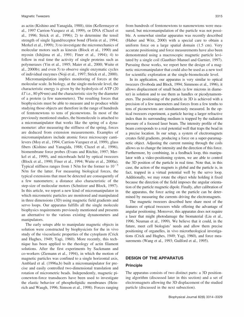
The six vertical coils (Fig. 2) are attached to a soft steel baseand are capped by curved pole pieces. The soft steel ring isdesigned to close the field lines in the system, thus increas-ing the magnitude of the magnetic field. A cylinder ofPlexiglas fixed at the pole-pieces end improves the mechan-ical cohesion of the apparatus.

The round piece closing the field lines is made of XC15soft steel (Tonnetot Metaux, Fontenay-sous-Bois, France)and the pole pieces are cylinders of mumetal (Goodfellow,Cambridge, U.K.). Those two alloys were chosen for theirlow remanent magnetization (20 gauss for mumetal). Coils(Lima 600880, Vizenza, Italy) are made of copper wire andhave a resistance of 10 � 0.2 . Each of them is driven bya current-power amplifier connected to the computer by adigital-to-analog converter. To avoid magnetic hysteresis,each change of the coil-driving current is accomplished withan exponentially decaying oscillating component added (theamplitude being the change size divided by two at each

FIGURE 1 General magnetic tweezers setup. A thin sample is observedwith an inverted microscope, a CCD image is processed by a computer thatdrives the electromagnets to servo the bead position in real time.

FIGURE 2 Detailed mechanical setup of the electromagnets. The sixcoils are placed in a hexagonal geometry, the magnetic field gradientsoccur between the tips of the mumetal pole pieces. With this configuration,the magnitude and direction of the force acting on the bead can be alteredby modulating the driving currents in the coils.

3316 Gosse and Croquette


period, i.e., every 4 ms). With low hysteresis materials, thismethod assigns a unique value of the magnetic field to thedriving current. A more sophisticated method has been usedin other experiments (Amblard et al., 1996b), where anactive control of the magnetic field through Hall probesfixed at the end of each pole piece feed back the current inthe associated coil.

Current configurations and bead movement

The coils have been designed to produce on the bead a forcewhose three components may be adjusted independently.Furthermore, various experimental constraints had to beovercome: the microscope objective and the light illumina-tion path did not allow placement of coils along the verticaloptical axis; some symmetry had to insure the rotationability. We have found that a set of six vertical electromag-nets placed in hexagonal pattern over the sample was ade-quate. However, the present system can only apply a forcedirected upward; the downward motion of the bead reliesupon gravity. This is certainly a limitation in this apparatus,but it can be overcome in the future by a more complex setof electromagnets. The six coils used here represent a min-imal system that, for the sake of simplicity, will be dis-cussed in this paper.

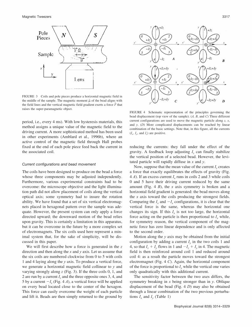
We will first describe how a force is generated in the zdirection and then along the x and y axis. Let us assume thatthe six coils are numbered clockwise from 0 to 5 with coils1 and 4 laying along the y axis. To produce a vertical force,we generate a horizontal magnetic field collinear to y andvarying strongly along z (Fig. 3). If the three coils 0, 1, and2 are run by a current Iz and the three opposite ones 3, 4, and5 by a current �Iz (Fig. 4 A), a vertical force will be appliedon every bead located close to the center of the hexagon.This force can easily overcome the weight of each particleand lift it. Beads are then simply returned to the ground by

reducing the currents: they fall under the effect of thegravity. A feedback loop adjusting Iz can finally stabilizethe vertical position of a selected bead. However, the levi-tated particle will rapidly diffuse in x and y.

Now, suppose that the mean value of the current Iz createsa force that exactly equilibrates the effects of gravity (Fig.4 A). If an excess current Ix runs in coils 2 and 3 while coils0 and 5 have their driving current reduced by the sameamount (Fig. 4 B), the x axis symmetry is broken and ahorizontal field gradient is generated: the bead moves alongthe x axis toward the coils producing the strongest fields.Comparing the Ix and �Ix configurations, it is clear that thevertical force is the same, whereas the horizontal onechanges its sign. If this Ix is not too large, the horizontalforce acting on the particle is then proportional to Ix while,for symmetry reason, the vertical component of the mag-netic force has zero linear dependence and is only affectedto the second order.

Motion along the y axis may be obtained from the initialconfiguration by adding a current Iy in the two coils 1 and4, so that Iz � Iy flows in 1 and �Iz � Iy in 4. The magneticfield is then reinforced around coil 1 and reduced aroundcoil 4: as a result the particle moves toward the strongestelectromagnet (Fig. 4 C). Again, the horizontal componentof the force is proportional to Iy while the vertical one variesonly quadratically with this additional current.

The sensitivity factor between the two axes differs, thesymmetry breaking in x being stronger than in y. Obliquedisplacement of the bead (Fig. 4 D) may also be obtainedthrough a linear combination of the two previous perturba-tions Ix and Iy (Table 1)

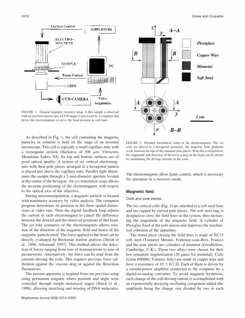
FIGURE 3 Coils and pole pieces produce a horizontal magnetic field inthe middle of the sample. The magnetic moment �� of the bead aligns withthe field lines and the vertical magnetic field gradient exerts a force F� thatraises the super-paramagnetic object.

FIGURE 4 Schematic representation of the principles governing thebead displacement (top view of the sample). (A, B, and C) Three differentcurrent configurations are used to move the magnetic particle along z, x,and y. (D) More complicated displacements can be reached by linearcombination of the basic settings. Note that, in this figure, all the currents(Ix, Iy, and Iz) are positive.



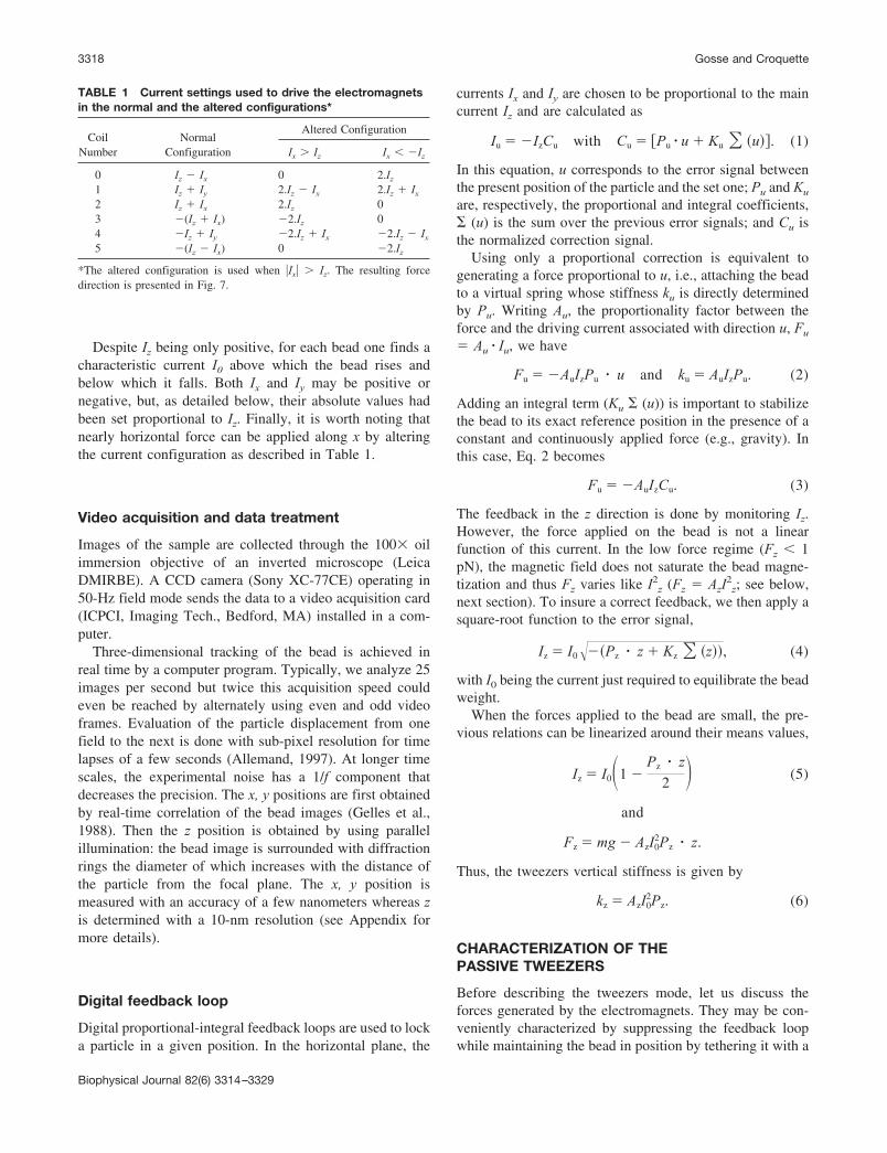
Despite Iz being only positive, for each bead one finds acharacteristic current I0 above which the bead rises andbelow which it falls. Both Ix and Iy may be positive ornegative, but, as detailed below, their absolute values hadbeen set proportional to Iz. Finally, it is worth noting thatnearly horizontal force can be applied along x by alteringthe current configuration as described in Table 1.

Video acquisition and data treatment

Images of the sample are collected through the 100 oilimmersion objective of an inverted microscope (LeicaDMIRBE). A CCD camera (Sony XC-77CE) operating in50-Hz field mode sends the data to a video acquisition card(ICPCI, Imaging Tech., Bedford, MA) installed in a com-puter.

Three-dimensional tracking of the bead is achieved inreal time by a computer program. Typically, we analyze 25images per second but twice this acquisition speed couldeven be reached by alternately using even and odd videoframes. Evaluation of the particle displacement from onefield to the next is done with sub-pixel resolution for timelapses of a few seconds (Allemand, 1997). At longer timescales, the experimental noise has a 1/f component thatdecreases the precision. The x, y positions are first obtainedby real-time correlation of the bead images (Gelles et al.,1988). Then the z position is obtained by using parallelillumination: the bead image is surrounded with diffractionrings the diameter of which increases with the distance ofthe particle from the focal plane. The x, y position ismeasured with an accuracy of a few nanometers whereas zis determined with a 10-nm resolution (see Appendix formore details).

Digital feedback loop

Digital proportional-integral feedback loops are used to locka particle in a given position. In the horizontal plane, the

currents Ix and Iy are chosen to be proportional to the maincurrent Iz and are calculated as

Iu � �IzCu with Cu � �Pu � u Ku � �u �. (1)

In this equation, u corresponds to the error signal betweenthe present position of the particle and the set one; Pu and Ku

are, respectively, the proportional and integral coefficients,� (u) is the sum over the previous error signals; and Cu isthe normalized correction signal.

Using only a proportional correction is equivalent togenerating a force proportional to u, i.e., attaching the beadto a virtual spring whose stiffness ku is directly determinedby Pu. Writing Au, the proportionality factor between theforce and the driving current associated with direction u, Fu

� Au � Iu, we have

Fu � �AuIzPu � u and ku � AuIzPu. (2)

Adding an integral term (Ku � (u)) is important to stabilizethe bead to its exact reference position in the presence of aconstant and continuously applied force (e.g., gravity). Inthis case, Eq. 2 becomes

Fu � �AuIzCu. (3)

The feedback in the z direction is done by monitoring Iz.However, the force applied on the bead is not a linearfunction of this current. In the low force regime (Fz � 1pN), the magnetic field does not saturate the bead magne-tization and thus Fz varies like I2

z (Fz � AzI2z; see below,

next section). To insure a correct feedback, we then apply asquare-root function to the error signal,

Iz � I0��Pz � z Kz � �z , (4)

with I0 being the current just required to equilibrate the beadweight.

When the forces applied to the bead are small, the pre-vious relations can be linearized around their means values,

Iz � I0�1 Pz � z

2 � (5)

and

Fz � mg AzI02Pz � z.

Thus, the tweezers vertical stiffness is given by

kz � AzI02Pz. (6)

CHARACTERIZATION OF THEPASSIVE TWEEZERS

Before describing the tweezers mode, let us discuss theforces generated by the electromagnets. They may be con-veniently characterized by suppressing the feedback loopwhile maintaining the bead in position by tethering it with a

TABLE 1 Current settings used to drive the electromagnetsin the normal and the altered configurations*

CoilNumber

NormalConfiguration

Altered Configuration

Ix � Iz Ix � �Iz

0 Iz � Ix 0 2.Iz

1 Iz � Iy 2.Iz � Ix 2.Iz � Ix

2 Iz � Ix 2.Iz 03 �(Iz � Ix) �2.Iz 04 �Iz � Iy �2.Iz � Ix �2.Iz � Ix

5 �(Iz � Ix) 0 �2.Iz

*The altered configuration is used when �Ix� � Iz. The resulting forcedirection is presented in Fig. 7.



DNA molecule. Indeed, this method allows application ofstrong forces in any direction.

We have prepared both � and pX�II DNA molecules(resp. �16 and 5 �m long) with one extremity labeled withdigoxigenin and the other with biotin. Incubating thesemolecules with streptavidin-coated super-paramagneticbeads 4.5 �m in diameter (Dynabeads, Dynal, Oslo, Nor-way) results in the attachment of the particle to the biotinend of the biopolymer. Injection of these beads into anantidigoxigenin-coated glass capillary allows the dioxigeninend of the DNA to attach to the tube surface.

Force measurements along z

We have first used the electromagnets configuration, whichproduces a force only along the z axis (Fig. 4 A). In thissituation, the bead behaves as an inverted pendulum im-mersed in a thermal bath at temperature T. As we haveshown in our previous work (Strick et al., 1996), the anal-ysis of the horizontal Brownian motion of the particlepermits measurement of the stretching force. More pre-cisely, the bead-positioning software determines the DNAextension l and the particle transverse fluctuations �x. Usingthe equipartition theorem, the vertical magnetic force Fmag

may then be evaluated through the simple formula, Fmag �kBTl/��x2� (Fig. 5).

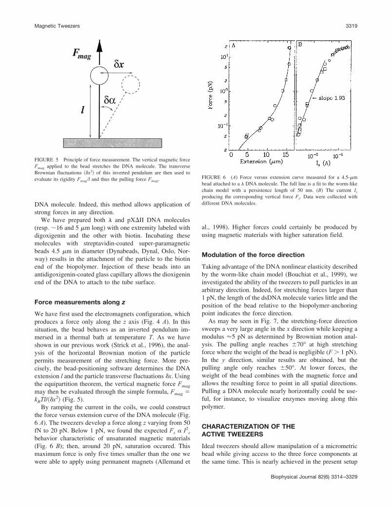
By ramping the current in the coils, we could constructthe force versus extension curve of the DNA molecule (Fig.6 A). The tweezers develop a force along z varying from 50fN to 20 pN. Below 1 pN, we found the expected Fz � I2

z

behavior characteristic of unsaturated magnetic materials(Fig. 6 B); then, around 20 pN, saturation occured. Thismaximum force is only five times smaller than the one wewere able to apply using permanent magnets (Allemand et

al., 1998). Higher forces could certainly be produced byusing magnetic materials with higher saturation field.

Modulation of the force direction

Taking advantage of the DNA nonlinear elasticity describedby the worm-like chain model (Bouchiat et al., 1999), weinvestigated the ability of the tweezers to pull particles in anarbitrary direction. Indeed, for stretching forces larger than1 pN, the length of the dsDNA molecule varies little and theposition of the bead relative to the biopolymer-anchoringpoint indicates the force direction.

As may be seen in Fig. 7, the stretching-force directionsweeps a very large angle in the x direction while keeping amodulus �5 pN as determined by Brownian motion anal-ysis. The pulling angle reaches �70° at high stretchingforce where the weight of the bead is negligible (F � 1 pN).In the y direction, similar results are obtained, but thepulling angle only reaches �50°. At lower forces, theweight of the bead combines with the magnetic force andallows the resulting force to point in all spatial directions.Pulling a DNA molecule nearly horizontally could be use-ful, for instance, to visualize enzymes moving along thispolymer.

CHARACTERIZATION OF THEACTIVE TWEEZERS

Ideal tweezers should allow manipulation of a micrometricbead while giving access to the three force components atthe same time. This is nearly achieved in the present setup

FIGURE 5 Principle of force measurement. The vertical magnetic forceFmag applied to the bead stretches the DNA molecule. The transverseBrownian fluctuations ��x2� of this inverted pendulum are then used toevaluate its rigidity Fmag/l and thus the pulling force Fmag. FIGURE 6 (A) Force versus extension curve measured for a 4.5-�m

bead attached to a � DNA molecule. The full line is a fit to the worm-likechain model with a persistence length of 50 nm. (B) The current Iz

producing the corresponding vertical force Fz. Data were collected withdifferent DNA molecules.



by recording the electromagnets driving currents. Neverthe-less, it is of course necessary to previously perform tweezerscalibration, i.e., to investigate the relation between currentsand forces. In the small-force regime, these relations arelinear, and thus the calibration consists of measuring thedifferent proportionality constants Au. These coefficientsvary from one magnetic bead to another. However, we willshow below that such a calibration can be achieved easilyby recording the particle fluctuations in the trapped statewith no external force applied.

To explain the tweezers properties and the related cali-bration procedure, we first introduce a simplified modelwith only an instantaneous proportional feedback. Thismodel depends only on two parameters: the tweezers elasticstiffness ku and the particle viscous drag coefficient ��r.We show that the analysis of the bead fluctuations in Fou-rier space allows determination of ��r at high frequenciesand ku at low frequencies. The measurement of ��r leads tothe viscosity of the fluid �, and the measurement of ku leadsto the Au through Eq. 2. Consequently, the tweezers may beused in two different operating modes: as a viscosimeter oras a dynamometer.

Finally, we discuss the properties of the real apparatuswith its slower digital feedback and its integral correction.In this case, the tweezers cannot be described anymore byour simplified model, but are better characterized by arecursive equation accounting for the servo loop delay.Within this new context, we present three complementarycalibration methods that provide absolute measurements ofthe force. Because the techniques and models used here aresometimes similar to the ones used for optical tweezers

calibration, the following analysis can be read in parallelwith the reviews, Svoboda and Block (1994), and Gittes andSchmidt (1998).

Model for ideal tweezers

To study the complete feedback loop of our apparatus, a4.5-�m super-paramagnetic bead is locked 10 �m above thesurface. As seen above, couplings among the x, y, and zforces are only quadratic, and, consequently, the three trap-ping directions may be considered as independent. For thesake of simplicity, we will also first work with a propor-tional feedback. Furthermore, we will assume that the feed-back presents no delay, which allows a simple description of“ideal” tweezers. The bead is locked in a virtual one-dimensional potential well where the magnetic tweezersrespond with a force Fu � � ku � u to a deviation u from theinitial set position. The equation of motion of the particlecan thereby be written,

md2u

dt ��r

du

dt kuu � FL, (7)

where m is the mass of the bead, r its radius, � the viscosityof the solution, and � the viscous drag coefficient (6� for aspherical object far from any surface). It is easy to verifythat the system is overdamped and the inertial term maythus be omitted. FL is the stochastic Langevin force respon-sible for the fluctuations characteristic of the Brownianmotion of the particle. From the fluctuation dissipationtheorem, it follows that �FL(t)� � 0 and �FL(t)FL(t�)� �2kBT��r�(t � t�), which appears as a white noise in Fourierspace, �FL(f)�2 � 4kBT��r. Note that this noise is also theintrinsic noise of our measurement.

In frequency space, the density of fluctuations is thengiven by

�u�f �2 �4kBT��r

�ku i��r2�f �2 � 4kBT��r

ku2

1

1 �f/fc 2, (8)

where fc � ku/(2��r). This power spectrum is a Lorent-zian corresponding to the response function of a bead at-tached to a spring, immersed in a viscous medium, andexcited by a white noise (the Langevin force). This noisedepends only on dissipative terms, it is proportional to � andr. More precisely, at low frequencies (f �� fc), the powerspectrum presents an asymptotic white noise determined bythe excitation of the spring ku through the Langevin noise,whereas, at high frequencies (f �� fc), the f�2 behavior isdominated by the viscous term ��r (Fig. 8 at small Pz

values).

Viscosimeter mode

Because, at high frequencies, the Brownian fluctuations ofthe bead presents a 1/f2 regime (see Fig. 8), the spectrum of

FIGURE 7 Positions of the bead center for the full range of x currentmodulation. The particle, 4.5 �m in diameter, is tethered to the glasssurface by a pX�II DNA molecule �5 �m long. The position of the beadand of the DNA molecule are drawn in vertical position and for themaximum modulations. The circle is a fit to the data points obtained formoderate modulation (�). These points are typically within 20 nm awayfrom the circle, demonstrating that the pulling force is unchanged. In theextreme modulations (E) the pulling direction is nearly horizontal and islimited by the fact that the bead touches the glass surface. For thoseextreme modulations, the stretching force decreases slightly as indi-cated by the shorter extension. The two long dashed lines indicate theboundary between the normal and the altered configuration of thecoil-driving currents (see Table 1).



the velocity fluctuations (the derivative Vu) presents anasymptotic white noise, the value of which is proportional tothe object diffusion coefficient D and thus inversely pro-portional to the viscous term ��r,

Vu2�f �� fc �

4kBT

��r� 4D. (9)

Consequently, the particle Brownian motion offers a simplemeans to use the magnetic tweezers as a viscosimeter invitro (Ziemann et al., 1994, Amblard et al., 1996b) or invivo (Crick and Hughes, 1949; Sato et al., 1984; Zaner andValberg, 1989, Yagi, 1960). First, the tweezers bring a beadto a specific point of interest. Then, the feedback is switchedto a low-stiffness mode, which allows measurement of thelocal viscosity while keeping the probe in a defined area.Accurate data may be obtained at such low-feedback pa-rameters because the cutoff frequency is small, leaving awide white-noise regime in the bead-velocity spectrum.Additionally, care must be taken to compensate for thevideo camera filtering due to exposure-integration dampingof the frequencies close to the acquisition rate.

Tweezers mode

The measure of ku leads to the calibration of the apparatus asa dynamometer. When the tweezers can be considered as ideal,

the calibration procedure can be achieved by using the equi-partition theorem. Provided that we record the bead fluctua-tions with an infinite frequency range, we can write kBT/2 �ku�u

2�/2 in real space. Thus, in Fourier space, we have

ku �kBT

�0�df �u�f �2. (10)

This calibration method is very powerful, but, as explainedbelow, it applies to the magnetic tweezers only when thevalues of the feedback parameters are low (i.e., when the Pu

are small). We will first discuss here the intrinsic limitationsof the method and its validity conditions. Then, we willshow that, although this method cannot be used directlywhen the values of the feedback parameters are high, it maybe adapted to this situation.

The two intrinsic limitations of the equipartition calibra-tion are finite bandwith and accuracy. In all experiments,the signal bandwidth is limited at high frequency to the halfof the sampling rate fs/2 and at low frequency to the inverseof the observation window fL � �T�1. Thus, the integrationlimits in Eq. 10 becomes fL and fs/2 instead of 0 and �. Tomaintain the accuracy of this relation, we must either ensurethat fs/2 �� fc �� fL or correct the equation from the limitedintegration range. This last method requires evaluation ofthe integral of the Lorentzian within the experimental rangeto determine fc.

Independently, it is worth noting that the estimation of fcis also useful to evaluate the statistical error on �u2� and thuson ku. To obtain good statistics and a precise measurementof the trap stiffness, Brownian motion must be recordedlong enough. ku is given with an accuracy of 1/N if thefluctuations are analyzed over a period N2 times largerthan 1/fc. In practice, we always adjust the measurementtime for reaching errors lower than 10%, for example, astiffness of 10�7 N/m (1/(2�fc) � 0.42 s) is evaluated witha 16,384-frames acquisition at 25 Hz, (total time �T �655 s), leading to an accuracy of �1/�fc�T � 6.5%.

In our experiment, as may be seen in Fig. 8, the spectraare indeed Lorentzian when the proportional feedback co-efficient Pu is not too large. In this regime, the simplifiedmodel of the tweezers may be applied, and the measure ofku using the equipartition theorem is valid (see Fig. 9).Nevertheless, as Pu is increased, this method does notremain valid anymore, and we can only use the low fre-quency asymptotic part of the spectrum to evaluate ku. Infact, it appears clearly that the value of the low-frequencywhite noise scales with Pu

�2, whereas the cutoff frequency fcincreases linearly. As a consequence, when Pu increases, thetrap characteristic time 1/(2�fc) decreases, and, above acritical value Puc, it becomes significant compared with thedelay in digital feedback (roughly two video frames). Res-onance then occurs, leading to an instability that forbidshigher feedback parameters and restrains the use of Eq. 10

FIGURE 8 Data points. Average power spectra of the vertical positionfluctuations of a trapped bead (only a variable proportional feedback isapplied here). These power spectra have a Lorentzian shape when thefeedback is small (top curves). As the feedback is increased, the fluctua-tions decrease and the cutoff frequency increases. At high feedback,ringing occurs (bottom curves). Solid lines. Power spectra obtained fromthe iterative model. L0

2, �, and � were first determined by fitting the lowestpower spectrum to Eq. 16 (� can only be evaluated when ringing occurs,i.e. at high Pz). The other spectra were then fitted while keeping L0

2 and �equal to the found values. Finally, the proportionality between � and Pz

(� � AzI02Pz�t/��r [Eqs. 6 and 13]) was checked.



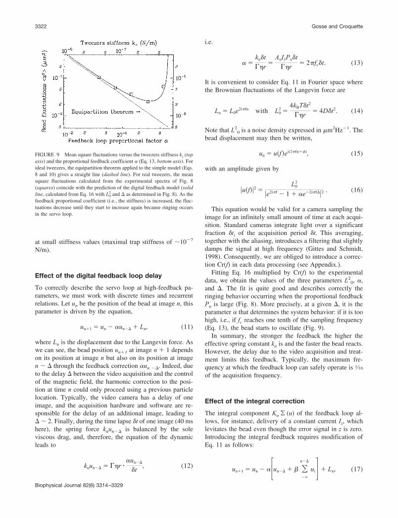
at small stiffness values (maximal trap stiffness of �10�7

N/m).

Effect of the digital feedback loop delay

To correctly describe the servo loop at high-feedback pa-rameters, we must work with discrete times and recurrentrelations. Let un be the position of the bead at image n, thisparameter is driven by the equation,

un�1 � un �un�� Ln, (11)

where Ln is the displacement due to the Langevin force. Aswe can see, the bead position un�1 at image n � 1 dependson its position at image n but also on its position at imagen � � through the feedback correction �un ��. Indeed, dueto the delay � between the video acquisition and the controlof the magnetic field, the harmonic correction to the posi-tion at time n could only proceed using a previous particlelocation. Typically, the video camera has a delay of oneimage, and the acquisition hardware and software are re-sponsible for the delay of an additional image, leading to� � 2. Finally, during the time lapse �t of one image (40 mshere), the spring force kuun�� is balanced by the soleviscous drag, and, therefore, the equation of the dynamicleads to

kuun�� r ��un��

�t, (12)

i.e.

� �ku�t

��r�

AuIzPu�t

��r� 2�fc�t. (13)

It is convenient to consider Eq. 11 in Fourier space wherethe Brownian fluctuations of the Langevin force are

Ln � L0e2i�fn with L0

2 �4kBT�t2

��r� 4D�t2. (14)

Note that L20 is a noise density expressed in �m2Hz�1. The

bead displacement may then be written,

un � u�f ei(2�fn��), (15)

with an amplitude given by

�u�f �2 �L0

2

�e2i�f 1 �e�2i�f��2 . (16)

This equation would be valid for a camera sampling theimage for an infinitely small amount of time at each acqui-sition. Standard cameras integrate light over a significantfraction �ti of the acquisition period �t. This averaging,together with the aliasing, introduces a filtering that slightlydamps the signal at high frequency (Gittes and Schmidt,1998). Consequently, we are obliged to introduce a correc-tion Cr(f) in each data processing (see Appendix.).

Fitting Eq. 16 multiplied by Cr(f) to the experimentaldata, we obtain the values of the three parameters L2

0, �,and �. The fit is quite good and describes correctly theringing behavior occurring when the proportional feedbackPu is large (Fig. 8). More precisely, at a given �, it is theparameter � that determines the system behavior: if it is toohigh, i.e., if fc reaches one tenth of the sampling frequency(Eq. 13), the bead starts to oscillate (Fig. 9).

In summary, the stronger the feedback the higher theeffective spring constant ku is and the faster the bead reacts.However, the delay due to the video acquisition and treat-ment limits this feedback. Typically, the maximum fre-quency at which the feedback loop can safely operate is 1⁄10

of the acquisition frequency.

Effect of the integral correction

The integral component Ku � (u) of the feedback loop al-lows, for instance, delivery of a constant current Iz, whichlevitates the bead even though the error signal in z is zero.Introducing the integral feedback requires modification ofEq. 11 as follows:

un�1 � un ��un��

n��

ui Ln, (17)

FIGURE 9 Mean square fluctuations versus the tweezers stiffness kz (topaxis) and the proportional feedback coefficient � (Eq. 13, bottom axis). Forideal tweezers, the equipartition theorem applied to the simple model (Eqs.8 and 10) gives a straight line (dashed line). For real tweezers, the meansquare fluctuations calculated from the experimental spectra of Fig. 8(squares) coincide with the prediction of the digital feedback model (solidline, calculated from Eq. 16 with L0

2 and � as determined in Fig. 8). As thefeedback proportional coefficient (i.e., the stiffness) is increased, the fluc-tuations decrease until they start to increase again because ringing occursin the servo loop.



with � � Ku/Pu. In Fourier space, this leads to

�u�f �2 �L0

2

e2i�f 1 �e�2i�f��1 i�ei�f

2 sin��f 2. (18)

Again, this is the response using an ideal camera. With areal camera, we must correct this equation by Cr(f) (see Eq.32). The coefficient � must be small because it introduces aphase shift. Proper values should be kept smaller than atenth. In these conditions, the lowest frequencies of the beadfluctuations are strongly filtered out (see Fig. 12 A) and thestability of the system is improved.

When the integral feedback is used, the stiffness of thetweezers ku depends on the frequency, and is thus not rigor-ously defined. However, we will still use ku to characterize thestiffness; this effective ku being the one measured if � is set tozero while all other parameters are kept constant.

Calibration against the viscous drag

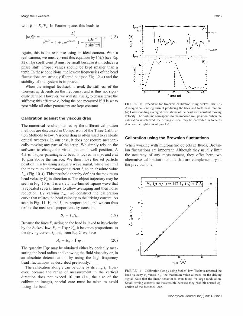
The numerical results obtained by the different calibrationmethods are discussed in Comparison of the Three Calibra-tion Methods below. Viscous drag is often used to calibrateoptical tweezers. In our case, it does not require mechani-cally moving any part of the setup. We simply rely on thesoftware to change the virtual potential well position. A4.5-�m super-paramagnetic bead is locked in x, y, and z at10 �m above the surface. We then move the set particleposition in u by using a square wave signal, while we limitthe maximum electromagnet current Iu to an absolute valueIum (Fig. 10 A). This threshold thereby defines the maximumbead velocity Vu in direction u. The object trajectory may beseen in Fig. 10 B, it is a slew rate-limited square wave thatis repeated several times to allow averaging and then noisereduction. By varying Ium, we construct the calibrationcurve that relates the bead velocity to the driving current. Asseen in Fig. 11, Vu and Iu are proportional, and we can thusdefine the measured proportionality constant,

Bu � Vu/Iu. (19)

Because the force Fu acting on the bead is linked to its velocityby the Stokes’ law, Fu � ��r � Vu, it becomes proportional tothe driving current Iu and, from Eq. 2, we have

Au � Bu � ��r. (20)

The quantity ��r may be obtained either by optically mea-suring the bead radius and knowing the fluid viscosity or, inan absolute determination, by using the high-frequencybead fluctuations as described previously.

The calibration along z can be done by driving Iz. How-ever, because the range of measurement in the verticaldirection does not exceed 10 �m (i.e., the size of thecalibration image), special care must be taken to avoidlosing the bead.

Calibration using the Brownian fluctuations

When working with micrometric objects in fluids, Brown-ian fluctuations are important. Although they usually limitthe accuracy of any measurement, they offer here twoalternative calibration methods that are complementary tothe previous one.

FIGURE 10 Procedure for tweezers calibration using Stokes’ law. (A)Averaged coil-driving current producing the back and forth bead motion.(B) Corresponding averaged oscillations of the bead with constant movingvelocity. The dash line corresponds to the imposed well position. When thecalibration is achieved, the driving current may be converted in force asdone on the right axis of panel A.

FIGURE 11 Calibration along y using Stokes’ law. We have reported thebead velocity Vy versus Iym, the maximum value allowed on the drivingsignal. Note that the linear behavior is even found for large modulation.Small driving currents are inaccessible because they prohibit normal op-eration of the feedback loop.



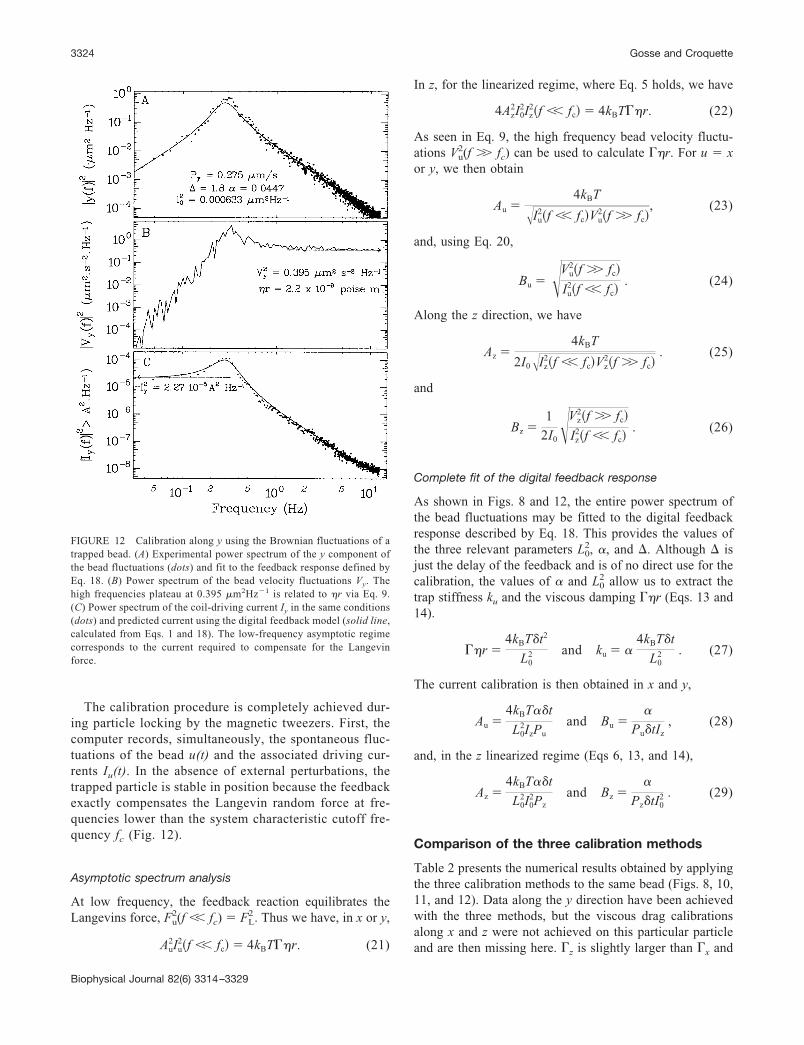
The calibration procedure is completely achieved dur-ing particle locking by the magnetic tweezers. First, thecomputer records, simultaneously, the spontaneous fluc-tuations of the bead u(t) and the associated driving cur-rents Iu(t). In the absence of external perturbations, thetrapped particle is stable in position because the feedbackexactly compensates the Langevin random force at fre-quencies lower than the system characteristic cutoff fre-quency fc (Fig. 12).

Asymptotic spectrum analysis

At low frequency, the feedback reaction equilibrates theLangevins force, Fu

2(f �� fc) � FL2. Thus we have, in x or y,

Au2Iu

2�f �� fc � 4kBT��r. (21)

In z, for the linearized regime, where Eq. 5 holds, we have

4Az2I0

2Iz2�f �� fc � 4kBT��r. (22)

As seen in Eq. 9, the high frequency bead velocity fluctu-ations Vu

2(f �� fc) can be used to calculate ��r. For u � xor y, we then obtain

Au �4kBT

�Iu2�f �� fc Vu

2�f �� fc , (23)

and, using Eq. 20,

Bu � �Vu2�f �� fc

Iu2�f �� fc

. (24)

Along the z direction, we have

Az �4kBT

2I0�Iz2�f �� fc Vz

2�f �� fc . (25)

and

Bz �1

2I0�Vz

2�f �� fc

Iz2�f �� fc

. (26)

Complete fit of the digital feedback response

As shown in Figs. 8 and 12, the entire power spectrum ofthe bead fluctuations may be fitted to the digital feedbackresponse described by Eq. 18. This provides the values ofthe three relevant parameters L0

2, �, and �. Although � isjust the delay of the feedback and is of no direct use for thecalibration, the values of � and L0

2 allow us to extract thetrap stiffness ku and the viscous damping ��r (Eqs. 13 and14).

��r �4kBT�t2

L02 and ku � �

4kBT�t

L02 . (27)

The current calibration is then obtained in x and y,

Au �4kBT��t

L02IzPu

and Bu ��

Pu�tIz, (28)

and, in the z linearized regime (Eqs 6, 13, and 14),

Az �4kBT��t

L02I0

2Pzand Bz �

�

Pz�tI02 . (29)

Comparison of the three calibration methods

Table 2 presents the numerical results obtained by applyingthe three calibration methods to the same bead (Figs. 8, 10,11, and 12). Data along the y direction have been achievedwith the three methods, but the viscous drag calibrationsalong x and z were not achieved on this particular particleand are then missing here. �z is slightly larger than �x and

FIGURE 12 Calibration along y using the Brownian fluctuations of atrapped bead. (A) Experimental power spectrum of the y component ofthe bead fluctuations (dots) and fit to the feedback response defined byEq. 18. (B) Power spectrum of the bead velocity fluctuations Vy. Thehigh frequencies plateau at 0.395 �m2Hz�1 is related to �r via Eq. 9.(C) Power spectrum of the coil-driving current Iy in the same conditions(dots) and predicted current using the digital feedback model (solid line,calculated from Eqs. 1 and 18). The low-frequency asymptotic regimecorresponds to the current required to compensate for the Langevinforce.



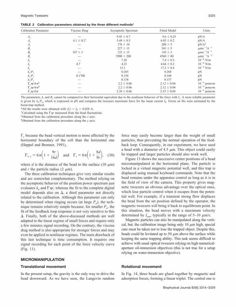
�y because the bead vertical motion is more affected by thehorizontal boundary of the cell than the horizontal one(Happel and Brenner, 1991),

�x, y � 6��1 9r

16d� and �z � 6��1 8d

9r�, (30)

where d is the distance of the bead to the surface (10 �m)and r the particle radius (2 �m).

The three calibration techniques give very similar resultsand are somewhat complementary. The method relying onthe asymptotic behavior of the position power spectrum justevaluates ku and ��r, whereas the fit to the complete digitalmodel depends also on �, a third parameter not directlyrelated to the calibration. Although this parameter can onlybe determined when ringing occurs (at large Pu), the tech-nique remains relatively simple because, for smaller Pu, thefit of the feedback loop response is not very sensitive to this�. Finally, both of the above-discussed methods are welladapted to the linear regime of small forces and require onlya few minutes signal recording. On the contrary, the viscousdrag method is also appropriate for stronger forces and mayeven be applied in nonlinear regimes. The main drawback ofthis last technique is time consumption. It requires onesignal recording for each point of the force velocity curve(Fig. 11).

MICROMANIPULATION

Translational movement

In the present setup, the gravity is the only way to drive thebead downward. As we have seen, the Langevin random

force may easily become larger than the weight of smallparticles, thus preventing the normal operation of the feed-back loop. Consequently, in our experiment, we have useda bead with a diameter of 4.5 �m. This object could easilybe trapped and larger particles should also work well.

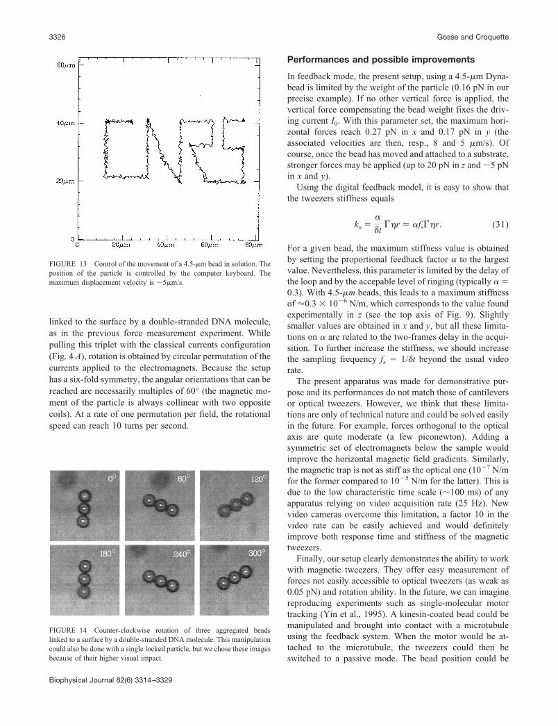
Figure 13 shows the successive center positions of a beadmicromanipulated in the horizontal plane. The particle islocked in a virtual magnetic potential well, and this trap isdisplaced using manual keyboard commands. Note that thebead remains under the apparatus control as long as it is inthe field of view of the camera. This property gives mag-netic tweezers an obvious advantage over the optical ones,which lose particle control when it escapes from the poten-tial well. For example, if a transient strong flow displacesthe bead from the set position defined by the operator, themagnetic tweezers will bring it back to equilibrium point. Inthis situation, the bead moves with a maximum velocitydetermined by Ium, typically in the range of 5–10 �m/s.

Magnetic particles can also be manipulated along the verti-cal, but, the calibration image being only 10 �m high, specialcare must be taken not to lose the trapped object. Despite this,beads could be levitated up to 50 �m above the surface whilekeeping the same trapping ability. This task seems difficult toachieve with usual optical tweezers relying on high numerical-aperture oil-immersion objectives (this is not true for a setuprelying on water-immersion objective).

Rotational movement

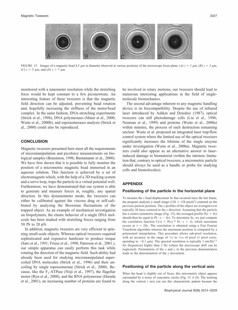
In Fig. 14, three beads are glued together by magnetic andadsorption forces, forming a linear triplet. The central one is

TABLE 2 Calibration parameters obtained by the three different methods*

Calibration Parameter Viscous Drag Asymptotic Spectrum Fitted Model Units

Ax — 9.45 � 0.7 9.6 � 0.25 pN/AAy 6.1 � 0.2† 5.49 � 0.5 6.03 � 0.2 pN/AAz — 176 � 10 200 � 5 pN/A2

Bx — 227 � 15 241 � 5 �ms�1A�1

By 147 � 3 132 � 15 145 � 3 �ms�1A�1

Bz — 3900 � 200 4560 � 80 �ms�1A�2

kx — 7.28 7.4 � 0.3 10�8 N/mky 4.7 4.23 4.64 � 0.2 10�8 N/mkz — 15.1 17.2 � 0.4 10�8 N/mkx/Px — 0.265 0.268 pNky/Py 0.1708 0.154 0.168 pNkz/Pz — 0.138 0.157 pN�x�r/6�‡ — 2.2 � 0.06 2.12 � 0.04 10�9 poise�m�y�r/6�§ — 2.2 � 0.06 2.12 � 0.04 10�9 poise�m�z�r/6� — 2.39 � 0.06 2.33 � 0.04 10�9 poise�m

The parameters Az and Bz cannot be compared to their horizontal equivalent due to the nonlinear behavior of the force with Iz. A more reliable parameteris given by ku/Pn, which is expressed in pN and compares the tweezers maximum force for the mean current I0. Errors on fits were estimated by theboost-trap method.*All the results were obtained with �Iz� � I0 � 0.028 A.†Calculated using the ��r measured from the bead fluctuations.‡Obtained from the calibration procedure along the x axis.§Obtained from the calibration procedure along the y axis.



linked to the surface by a double-stranded DNA molecule,as in the previous force measurement experiment. Whilepulling this triplet with the classical currents configuration(Fig. 4 A), rotation is obtained by circular permutation of thecurrents applied to the electromagnets. Because the setuphas a six-fold symmetry, the angular orientations that can bereached are necessarily multiples of 60° (the magnetic mo-ment of the particle is always collinear with two oppositecoils). At a rate of one permutation per field, the rotationalspeed can reach 10 turns per second.

Performances and possible improvements

In feedback mode, the present setup, using a 4.5-�m Dyna-bead is limited by the weight of the particle (0.16 pN in ourprecise example). If no other vertical force is applied, thevertical force compensating the bead weight fixes the driv-ing current I0. With this parameter set, the maximum hori-zontal forces reach 0.27 pN in x and 0.17 pN in y (theassociated velocities are then, resp., 8 and 5 �m/s). Ofcourse, once the bead has moved and attached to a substrate,stronger forces may be applied (up to 20 pN in z and �5 pNin x and y).

Using the digital feedback model, it is easy to show thatthe tweezers stiffness equals

ku ��

�t��r � �fs��r. (31)

For a given bead, the maximum stiffness value is obtainedby setting the proportional feedback factor � to the largestvalue. Nevertheless, this parameter is limited by the delay ofthe loop and by the accepable level of ringing (typically � �0.3). With 4.5-�m beads, this leads to a maximum stiffnessof �0.3 10�6 N/m, which corresponds to the value foundexperimentally in z (see the top axis of Fig. 9). Slightlysmaller values are obtained in x and y, but all these limita-tions on � are related to the two-frames delay in the acqui-sition. To further increase the stiffness, we should increasethe sampling frequency fs � 1/�t beyond the usual videorate.

The present apparatus was made for demonstrative pur-pose and its performances do not match those of cantileversor optical tweezers. However, we think that these limita-tions are only of technical nature and could be solved easilyin the future. For example, forces orthogonal to the opticalaxis are quite moderate (a few piconewton). Adding asymmetric set of electromagnets below the sample wouldimprove the horizontal magnetic field gradients. Similarly,the magnetic trap is not as stiff as the optical one (10�7 N/mfor the former compared to 10�5 N/m for the latter). This isdue to the low characteristic time scale (�100 ms) of anyapparatus relying on video acquisition rate (25 Hz). Newvideo cameras overcome this limitation, a factor 10 in thevideo rate can be easily achieved and would definitelyimprove both response time and stiffness of the magnetictweezers.

Finally, our setup clearly demonstrates the ability to workwith magnetic tweezers. They offer easy measurement offorces not easily accessible to optical tweezers (as weak as0.05 pN) and rotation ability. In the future, we can imaginereproducing experiments such as single-molecular motortracking (Yin et al., 1995). A kinesin-coated bead could bemanipulated and brought into contact with a microtubuleusing the feedback system. When the motor would be at-tached to the microtubule, the tweezers could then beswitched to a passive mode. The bead position could be

FIGURE 13 Control of the movement of a 4.5-�m bead in solution. Theposition of the particle is controlled by the computer keyboard. Themaximum displacement velocity is �5�m/s.

FIGURE 14 Counter-clockwise rotation of three aggregated beadslinked to a surface by a double-stranded DNA molecule. This manipulationcould also be done with a single locked particle, but we chose these imagesbecause of their higher visual impact.



monitored with a nanometer resolution while the stretchingforce would be kept constant to a few piconewtons. Aninteresting feature of these tweezers is that the magneticfield direction can be adjusted, preventing bead rotationand, hopefully increasing the stiffness of the motor/beadcomplex. In the same fashion, DNA-stretching experiments(Strick et al., 1998), DNA polymerases (Maier et al., 2000;Wuite et al., 2000b), and topoisomerases analysis (Strick etal., 2000) could also be reproduced.

CONCLUSION

Magnetic tweezers presented here meet all the requirementsof micromanipulation and picoforce measurements on bio-logical samples (Bensimon, 1996; Bustamante et al., 2000).We have first shown that it is possible to fully monitor theposition of a micrometric magnetic bead immersed in anaqueous solution. This function is achieved by a set ofelectromagnets which, with the help of a 3D tracking systemand a servo loop, traps the particle in a virtual potential well.Furthermore, we have demonstrated that our system is ableto generate and measure forces in, roughly, any spatialdirection. In this dynamometer mode, the tweezers caneither be calibrated against the viscous drag or self-cali-brated by analyzing the Brownian fluctuations of thetrapped object. As an example of mechanical investigationon biopolymers, the elastic behavior of a single DNA mol-ecule has been studied with stretching forces ranging from50 fN to 20 pN.

In addition, magnetic tweezers are very efficient in spin-ning small-scale objects. Whereas optical tweezers requiredsophisticated and expensive hardware to produce torque(Sato et al., 1991; Friese et al., 1998; Paterson et al., 2001.),our simple apparatus can easily perform this task whilerotating the direction of the magnetic field. Such ability hadalready been used for studying micromanipulated super-coiled DNA molecules (Strick et al., 1996) and their un-coiling by single topoisomerase (Strick et al., 2000). Be-cause, like the F1-ATPase (Noji et al., 1997), the flagellarmotor (Ryu et al., 2000), and the RNA polymerase (Haradaet al., 2001), an increasing number of proteins are found to

be involved in rotary motions, our tweezers should lead tonumerous interesting applications in the field of single-molecule biomechanics.

The second advantage inherent to any magnetic handlingdevice is its biocompatibility. Despite the use of infraredlaser introduced by Ashkin and Dziedzic (1987), opticaltweezers can still photodamage cells (Liu et al., 1996;Neuman et al., 1999) and proteins (Wuite et al., 2000a)within minutes, the process of such destruction remainingunclear. Wuite et al. proposed an integrated laser trap/flowcontrol system where the limited use of the optical tweezerssignificantly increases the lifetime of the single enzymeunder investigation (Wuite et al., 2000a). Magnetic twee-zers could also appear as an alternative answer to laser-induced damage to biomaterial (within the intrinsic limita-tion that, contrary to optical tweezers, a micrometric particleshould always be used as a handle or probe for studyingcells and biomolecules).

APPENDIX

Positioning of the particle in the horizontal plane

To measure the x bead displacement �x that occurred since the last frame,the program analyzes a small image (128 128 pixels2) centered on theprevious particle position. The x profiles of the object are averaged overtypically 20 lines centered in the y direction. Assuming that the particlehas a centro-symmetric image (Fig. 15), the averaged profile P(x � �x)should then be equal to P(�x � �x). To determine �x, we just computethe correlation function C( ) � P(x) * P(�x � ), which maximumoccurs at � 2�x. The correlation is obtained using a Fast FourierTransform algorithm whereas the maximum position is computed by apolynomial interpolation. This procedure allows sub-pixel resolution,with an accuracy in the range of 1⁄10 to 1⁄100 of pixel (1 pixel corre-sponding to �0.1 �m). The spectral resolution is typically 1 nm/Hz1/2

for frequencies higher than 2 Hz (where the microscope drift can beneglected). Permutation of the x and y in the previous demonstrationleads to the determination of the y movement.

Positioning of the particle along the vertical axis

When the bead is slightly out of focus, this micrometric object appearssurrounded by a series of concentric circles (Fig. 15 A–D). The trackingalong the vertical z axis can use this characteristic pattern because the

FIGURE 15 Images of a magnetic bead 4.5 �m in diameter observed at various positions of the microscope focus plane: (A) z � 1 �m, (B) z � 3 �m,(C) z � 5 �m, and (D) z � 7 �m.



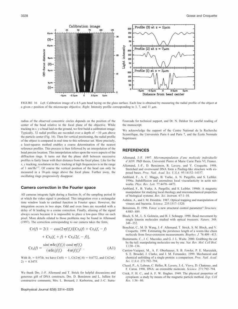
radius of the observed concentric circles depends on the position of thecenter of the bead relative to the focal plane of the objective. Whiletracking in x, y a bead laid on the ground, we first build a calibration image.Typically, 32 radial profiles are recorded over a depth of �10 �m abovethe particle center (Fig. 16). Then for vertical positioning, the radial profileof the object is compared in real time to this reference set. More precisely,a least-squares method enables a coarse determination of the nearestreference profiles. This process is then followed by an interpolation of thebead precise location. This interpolation relies upon the wave aspects of thediffraction rings. It turns out that the phase shift between successiveprofiles is fairly linear with their distance from the focal plane. Like for thex, y tracking, resolution in the z tracking at high frequencies is in the rangeof 1 nm/Hz1/2. Of course the vertical position of the bead can only bemeasured in a 10-�m range above the focal plane. Further away, theoscillating rings progressively disappear.

Camera correction in the Fourier space

All cameras integrate light during a fraction �ti of the sampling period �tat which the video signal is produced. This integration over a rectangulartime window leads to cardinal function in Fourier space. However, theintegration occurs in two steps. Odd and even lines are recorded with adelay of �t leading to a cosine correction. Finally, aliasing of the signalalways occurs because it is impossible to place a low-pass filter on eachpixel. More details related to those problems may be found in Allemand(1997). The correction corresponding to our camera takes the form,

Cr�f � 2�1 cos�2�f/fs �Cr0�f Cr0�fs f

Cr0�fs f Cr0�2fs f ] ,

Cr0�f �sin��ti�f/fs

��ti�f/fs

cos��f/fs

4��f/fs 2 . (A1)

With �ti � 0.97�t, we have Cr(0) � 1, Cr(2�fs/4) � 0.6772, and Cr(2�fs/2) � 0.3475.

We thank Drs. J.-F. Allemand and T. Strick for helpful discussions andgenerous gift of DNA constructs, Drs. D. Bensimon and L. Jullien forconstructive comments, Mrs. L. Brouard, J. Kerboriou, and J.-C. Sutra-

Fourcade for technical support, and Dr. N. Dekker for careful reading ofthe manuscript.

We acknowledge the support of the Centre National de la RechercheScientifique, the Universites Paris 6 and Paris 7, and the Ecole NormaleSuperieure.

REFERENCES

Allemand, J.-F. 1997. Micromanipulation d’une molecule individuelled’ADN. PhD thesis, Universite Pierre et Marie Curie Paris VI, France.

Allemand, J.-F., D. Bensimon, R. Lavery, and V. Croquette. 1998.Stretched and overwound DNA form a Pauling-like structure with ex-posed bases. Proc. Natl. Acad. Sci. U.S.A. 95:14152–14157.

Amblard, F., A. C. Maggs, B. Yurke, A. N. Pargellis, and S. Leibler.1996a. Subdiffusion and anomalous local viscoelasticity in actin net-works. Phys. Rev. Lett. 77:4470–4473.

Amblard, F., B. Yurke, A. Pargellis, and S. Leibler. 1996b. A magneticmanipulator for studying local rheology and micromechanical propertiesof biological systems. Rev. Sci. Instrum. 67:1–10.

Ashkin, A., and J. M. Dziedzic. 1987. Optical trapping and manipulation ofviruses and bacteria. Science. 235:1517–1520.

Bensimon, D. 1996. Force: a new structural control parameter? Structure.4:885–889.

Block, S. M., L. S. Golstein, and B. J. Schnapp. 1990. Bead movement bysingle kinesin molecules studied with optical tweezers. Nature. 348:348–352.

Bouchiat, C., M. D. Wang, J.-F. Allemand, T. Strick, S. M. Block, and V.Croquette. 1999. Estimating the persitence length of a worm-like chainmolecule from force-extension measurements. Biophys. J. 76:409–413.

Bustamante, C., J. C. Macosko, and G. J. L. Wuite. 2000. Grabbing the catby the tail: manipulating molecules one by one. Nat. Rev. Mol. Cell Biol.1:130–136.

Carrion-Vazquez, M., A. F. Oberhauser, S. B. Fowler, P. E. Marszalek,S. E. Broedel, J. Clarke, and J. M. Fernandez. 1999. Mechanical andchemical unfolding of a single protein: a comparison. Proc. Natl. Acad.Sci. U.S.A. 271:792–794.

Cluzel, P., A. Lebrun, C. Heller, R. Lavery, J.-L. Viovy, D. Chatenay, andF. Caron. 1996. DNA: an extensible molecule. Science. 271:792–794.

Crick, F. H. C., and A. F. W. Hughes. 1949. The physical properties ofcytoplasm: a study by means of the magnetic particle method. Exp. CellRes. 1:36–80.

FIGURE 16 Left. Calibration image of a 4.5-�m bead laying on the glass surface. Each line is obtained by measuring the radial profile of the object ata given z position of the microscope objective. Right. Intensity profile corresponding to 3, 7, and 11 �m.



Evans, E., and K. Ritchie. 1997. Dynamic strength of molecular adhesionbonds. Biophys. J. 72:1541– 1555.

Finer, J. T., R. M. Simmons, and J. A. Spudich. 1994. Single myosinmolecule mechanics: piconewtons and nanometre steps. Nature. 368:113–119.

Florin, E.-L., V. T. Moy, and H. E. Gaub. 1994. Adhesion force betweenindividual ligand–receptor pairs. Science. 264:415–417.

Friese, M. E. J., T. A. Nieminen, N. R. Heckenberg, and H. Rubinsztein-Dunlop. 1998. Optical alignment and spinning of laser-trapped micro-scopic particles. Nature. 394:348–350.

Gauthier-Manuel, B., and L. Garnier. 1997. Design for a 10 picometermagnetic actuator. Rev. Sci. Instrum., 68:2486–2489.

Gelles, J., B. Schnapp, and M. Sheetz. 1988. Tracking kinesin-drivenmovements with nanometre-scale precision. Nature. 331:450–453.

Gittes, F., and C. F. Schimdt. 1998. Signals and noise in micromechanicalmeasurements. Methods Cell Biol. 55:129–156.

Guilford, W. H., R. C. Lantz, and R. W. Gore. 1995. Locomotive forcesproduced by single leukocytes in vivo and in vitro. Am. J. Physiol. (CellPhysiol). 268:C1308–C1312.

Haber, C., and D. Witz. 2000. Magnetic tweezers for DNA micromanip-ulation. Rev. Sci. Inst. 71:4561–4569.

Harada, Y., O. Ohara, A. Takatsuki, H. Itoh, N. Shimamoto, and K.Kinosita. 2001. Direct observation of DNA rotation during transcriptionby Escherichia coli RNA polymerase. Nature. 409:113–115.

Happel, J., and H. Brenner. 1991. Low Reynolds Number Hydrodynamics.Kluwer Academics, Boston, MA.

Heinrich, W., and R. E. Waugh. 1996. A piconewton force transducer andits application to the measurement of the bending stiffness of thephospholipid membranes. Ann. Biomed. Eng. 24:595–605.

Ishijima, A., T. Doi, K. Sakurada, and T. Yanagida. 1991. Sub-piconewtonforce fluctuations of the actomyosin in vitro. Nature. 352:301–306.

Kellermayer, M. S. Z., S. B. Smith, H. L. Granzier, and C. Bustamante.1997. Folding-unfolding transitions in single titin molecules character-ized with laser tweezers. Science. 276:1112–1116.

Kishino, A., and T. Yanagida. 1988. Force measurement by micromanip-ulation of a single actin filament by glass needles. Nature. 334:74–76.

Liu, Y., G. J. Sonek, M. W. Berns, and B. J. Tromberg. 1996. Physiologicalmonitoring of optically trapped cells: effects of the confinement by1064-nm laser tweezers using microfluorometry. Biophys. J. 71:2158–2167.

Maier, B., D. Bensimon, and V. Croquette. 2000. Replication by a singleDNA-polymerase of a stretched single strand DNA. Proc. Natl. Acad.Sci. U.S.A. 97:12002–12007.

Merkel, R., P. Nassoy, A. Leung, K. Ritchie, and E. Evans. 1999. Energylandscapes of receptor–ligand bonds explored with dynamic force spec-troscopy. Nature. 397:50–53.

Moy, V. T., E.-L. Florin, and H. E. Gaub. 1994. Intermolecular forces andenergies between ligands and receptors. Science. 266:257–259.

Neuman, K. C., E. H. Chadd, G. F. Liou, K. Bergman, and S. M. Block.1999. Characterization of photo-damage to Escherichia coli in opticaltraps. Biophys. J. 77:2856–2863.

Noji, H., R. Yasuda, M. Yoshida, and K. Kinosita. 1997. Direct observa-tion of the rotation of F1-ATPase. Nature. 386:299–302.

Paterson, L., M. P. MacDonald, J. Arlt, W. Sibbett, P. E. Bryant, and K.Dholakia. 2001. Controlled rotation of optically trapped microscopicparticles. Science. 292:912–914.

Ryu, W. S., R. M. Berry, and H. C. Berg. 2000. Torque-generating units ofthe flagellar motor of Escherichia coli have a high duty ratio. Nature.403:444–447.

Sato, M., T. Z. Wong, D. T. Brown, and R. D. Allen. 1984. Rheologicalproperties of living cytoplasm: a preliminary investigation of squidaxoplasm (Loligo peali). Cell Mobility. 4:7–23.

Sato, S., M. Ishigure, and H. Inaba. 1991. Optical trapping and rotationalmanipulation of microscopic particles and biological cells using higher-order mode Nd:Yag laser beams. Electronics Lett. 27:1831– 1832.

Schnitzer, M. J., and S. Block. 1997. Kinesin hydrolyses one ATP per 8-nmstep. Nature. 388:386–390.

Simmons, R. M., J. T. Finer, S. Chu, and J. A. Spudich. 1996. Quantitativemeasurements of force and displacement using an optical trap.Biophys. J. 70:1813–1822.

Simson, D. A., F. Ziemann, M. Strigl, and R. Merkel. 1998. Micropipet-based pico force transducer: in depth analysis and experimental verifi-cation. Biophys. J. 74:2080–2088.

Strick, T. R., J.-F. Allemand, D. Bensimon, A. Bensimon, and V. Cro-quette. 1996. The elasticity of a single supercoiled DNA molecule.Science. 271:1835–1837.

Strick, T. R., J.-F. Allemand, D. Bensimon, and V. Croquette. 1998. Thebehavior of supercoiled DNA. Biophys. J. 74:2016–2028.

Strick, T. R., V. Croquette, and D. Bensimon. 2000. Single-moleculeanalysis of DNA uncoiling by a type II topoisomerase. Nature. 404:901–904.

Svoboda, K., and S. M. Block. 1994. Biological applications of opticalforces. Annu. Rev. Biophys. Biomol. Struct. 23:247–285.

Wang, N., J. P. Butler, and D. E. Ingber. 1993. Mechanotransductionacross the cell surface and through the cytoskeleton. Science. 260:1124–1127.

Wuite, G. J. L., R. J. Davenport, A. Rappaport, and C. Bustamante. 2000a.An integrated laser trap/flow control video microscope for the study ofsingle biomolecules. Biophys. J. 79:1155–1167.

Wuite, G. J., S. B. Smith, M. Young, D. Keller, and C. Bustamante. 2000b.Single-molecule studies of the effect of template tension on T7 DNApolymerase activity. Nature. 404:103–106.

Yagi, K. 1960. The mechanical and colloidal properties of amoeba proto-plasm and their relations to the mechanism of amoeboid movement.Comp. Biochem. Physiol. 3:73–91.

Yin, H., M. P. Wang, K. Svoboda, R. Landick, S. M. Block, and J. Gelles.1995. Transcription against an applied force. Science. 270:1653–1657.

Zaner, K. S., and P. A. Valberg. 1989. Viscoelasticity of F-actin measuredwith magnetic microparticles. J. Cell Biol. 109:2233–2243.

Ziemann, F., J. Radler, and E. Sackmann. 1994. Local measurements of theviscoelastic moduli of entangled actin networks using an oscillatingmagnetic bead micro-rheometer. Biophys. J. 66:2210–2216.



magnetic tweezers: micromanipulation and force measurement ... · magnetic tweezers:...

Documents