measurement, modeling, and characterization for power
TRANSCRIPT

THESIS FOR THE DEGREE OF LICENTIATE OF ENGINEERING
Measurement, Modeling, andCharacterization for Power-Aware
Computing
BHAVISHYA GOEL
Division of Computer EngineeringDepartment of Computer Science and Engineering
CHALMERS UNIVERSITY OF TECHNOLOGY
Göteborg, Sweden 2014

Measurement, Modeling, and Characterization for Power-Aware ComputingBhavishya Goel
Copyright c© Bhavishya Goel, 2014.
Technical report 111LISSN 1652-876XDepartment of Computer Science and EngineeringComputer Architecture Research Group
Division of Computer EngineeringChalmers University of TechnologySE-412 96 GÖTEBORG, SwedenPhone: +46 (0)31-772 10 00
Author e-mail: [email protected]
Chalmers ReposerviceGöteborg, Sweden 2014

Measurement, Modeling, and Characterization for Power-AwareComputing
Bhavishya GoelDivision of Computer Engineering, Chalmers University of Technology
ABSTRACTSociety’s increasing dependence on information technology has resulted in thedeployment of vast compute resources. The energy costs of operating theseresources coupled with environmental concerns have made power-aware com-puting one of the primary challenges for the IT sector. Making energy-efficientcomputing a rule rather than an exception requires that researchers and systemdesigners use the right set of techniques and tools. These involve measuring,modeling, and characterizing the energy consumption of computers at varyingdegrees of granularity.
In this thesis, we present techniques to measure power consumption of com-puter systems at various levels. We compare them for accuracy and sensitiv-ity and discuss their effectiveness. We test Intel’s hardware power model forestimation accuracy and show that it is fairly accurate for estimating energyconsumption when sampled at the temporal granularity of more than tens ofmilliseconds.
We present a methodology to estimate per-core processor power consump-tion using performance counter and temperature-based power modeling and val-idate it across multiple platforms. We show our model exhibits negligible com-putation overhead, and the median estimation errors ranges from 0.3% to 10.1%for applications from SPEC2006, SPEC-OMP and NAS benchmarks. We testthe usefulness of the model in a meta-scheduler to enforce power constraint ona system.
Finally, we perform a detailed performance and energy characterization ofIntel’s Restricted Transactional Memory (RTM). We use TinySTM softwaretransactional memory (STM) system to benchmark RTM’s performance againstcompeting STM alternatives. We use microbenchmarks and STAMP bench-mark suite to compare RTM versus STM performance and energy behavior. Wequantify the RTM hardware limitations that affect its success rate. We showthat RTM performs better than TinySTM when working-set fits inside the cacheand that RTM is better at handling high contention workloads.
Keywords: power estimation, energy characterization, power-aware scheduling, power
management, transactional memory, power measurement

ii

Preface
Parts of the contributions presented in this thesis have previously been publishedin the following manuscripts.
. Bhavishya Goel, Sally A. McKee, Roberto Gioiosa, Karan Singh,Major Bhadauria, Marco Cesati, “Portable, Scalable, Per-Core PowerEstimation for Intelligent Resource Management” in Proceedingsof the 1st International Green Computing Conference, Chicago,USA, August, 2010, pp.135-146.
. Bhavishya Goel, Sally A. McKee, Magnus Själander, “Techniquesto Measure, Model, and Manage Power,” in Advances in Comput-ers 87, 2012, pp.7-54.
The following manuscript has been accepted but is yet to be published.
. Bhavishya Goel, Ruben Titos-Gil, Anurag Negi, Sally A. Mc-Kee, Per Stenstrom, “Performance and Energy Analysis of the Re-stricted Transactional Memory Implementation on Haswell” To ap-pear in Proceedings of 28th IEEE International Parallel and Dis-tributed Processing Symposium, Phoenix, USA, May, 2014.
The following manuscripts have been published but are not included in thiswork.
. Bhavishya Goel, Magnus Själander, Sally A. McKee, “RTL Modelfor Dynamically Resizable L1 Data Cache” in Swedish System-on-Chip Conference, Ystad, Sweden, 2013
. Magnus Själander, Sally A. McKee, Bhavishya Goel, Peter Brauer,David Engdal, Andras Vajda, “Power-Aware Resource Scheduling
iii

PREFACE iv
in Base Stations” in 19th Annual IEEE/ACM International Sym-posium on Modeling, Analysis and Simulation of Computer andTelecommunication Systems, Singapore, Singapore, July, 2012, pp.462-465.

Acknowledgments
I will like to thank following people for supporting me during my researchcareer and playing their part in bringing this thesis to fruition.
. Professor Sally A. McKee for inspiring me to join the computer archi-tecture research field and giving me the opportunity to work with her.She has been a great adviser and even greater friend. She is alwaysready to help out with any problems that I bring to her, technical or non-technical, and it is easy to say that I owe my research career to her. Sheis also an excellent cook and her brownies and palak paneers have gotme through various deadlines.
. Magnus Själander for helping me with my research and providing megreat technical feedback whenever we worked together. His enthusiasmfor research is very contagious and has helped me in keeping myselfmotivated.
. Professor Per Larsson-Edefors for teaching some of the most entertain-ing courses I have taken at Chalmers and for his valuable feedback fromtime to time.
. Professor Lars Svensson for helping me with practical issues during histime as division head.
. Professor Per Stenström for introducing me to the field of computer ar-chitecture and being an inspiration.
. Ruben and Anurag for being wonderful co-authors and helping me ingetting started with the basics of transactional memory.
. Karan Singh, Vincent M. Weaver and Major Bhadauria for getting mestarted with the power modeling infrastructure at Cornell and answeringmy naïve questions patiently.
v

ACKNOWLEDGMENTS vi
. Roberto Gioiosa and Marco Cesati for helping me run experiments formy first paper.
. Madhavan and Jacob for sharing office space with me and listening tomy jokes and rants.
. Alen, Angelos, Dmitry, Kasyab, Gabriele, Vinay, and Jochen for beingwonderful colleagues and friends and for making me look forward tocome to work.
. All the colleagues and staff at Computer Science and Engineering de-partment for creating a healthy work environment.
. Anthony Brandon for giving me valuable support when I was workingwith ρVEX processor for ERA project.
. Eva Axelsson, Tiina Rankanen, Jonna Amgard and Marianne Pleen-Shreiber for providing excellent administrative support during my timeat Chalmers.
. European Union for funding my research.
. My parents for supporting my career decisions and being great parentsin general.
Bhavishya GoelGöteborg, March 2014

Contents
Abstract i
Preface iii
Acknowledgments v
1 Introduction 21.1 Power Measurement . . . . . . . . . . . . . . . . . . . . . . . 31.2 Power Modeling . . . . . . . . . . . . . . . . . . . . . . . . . . 41.3 Power Characterization . . . . . . . . . . . . . . . . . . . . . . 51.4 Thesis Organization . . . . . . . . . . . . . . . . . . . . . . . . 6
2 Power Measurement Techniques 72.1 Overview . . . . . . . . . . . . . . . . . . . . . . . . . . . . . 72.2 Power Measurement Techniques . . . . . . . . . . . . . . . . . 8
2.2.1 At the Wall Outlet . . . . . . . . . . . . . . . . . . . . 82.2.2 At the ATX Power Rails . . . . . . . . . . . . . . . . . 92.2.3 At the Processor Voltage Regulator . . . . . . . . . . . 112.2.4 Experimental Results . . . . . . . . . . . . . . . . . . . 13
2.3 RAPL power estimations . . . . . . . . . . . . . . . . . . . . . 182.3.1 Overview . . . . . . . . . . . . . . . . . . . . . . . . . 182.3.2 Experimental Results . . . . . . . . . . . . . . . . . . . 18
2.4 Related Work . . . . . . . . . . . . . . . . . . . . . . . . . . . 232.5 Conclusion . . . . . . . . . . . . . . . . . . . . . . . . . . . . 24
3 Per-core Power Estimation Model 253.1 Overview . . . . . . . . . . . . . . . . . . . . . . . . . . . . . 25
vii

CONTENTS viii
3.2 Modeling Approach . . . . . . . . . . . . . . . . . . . . . . . . 293.3 Methodology . . . . . . . . . . . . . . . . . . . . . . . . . . . 30
3.3.1 Counter Selection . . . . . . . . . . . . . . . . . . . . . 303.3.2 Model Formation . . . . . . . . . . . . . . . . . . . . . 34
3.4 Validation . . . . . . . . . . . . . . . . . . . . . . . . . . . . . 363.4.1 Computation Overhead . . . . . . . . . . . . . . . . . . 383.4.2 Estimation Error . . . . . . . . . . . . . . . . . . . . . 38
3.5 Management . . . . . . . . . . . . . . . . . . . . . . . . . . . 443.5.1 Sample Policies . . . . . . . . . . . . . . . . . . . . . . 453.5.2 Experimental Setup . . . . . . . . . . . . . . . . . . . . 463.5.3 Results . . . . . . . . . . . . . . . . . . . . . . . . . . 473.5.4 Related Work . . . . . . . . . . . . . . . . . . . . . . . 48
3.6 Conclusion . . . . . . . . . . . . . . . . . . . . . . . . . . . . 51
4 Characterization of Intel’s Restricted Transactional Memory 524.1 Introduction . . . . . . . . . . . . . . . . . . . . . . . . . . . . 524.2 Experimental Setup . . . . . . . . . . . . . . . . . . . . . . . . 534.3 Microbenchmark analysis . . . . . . . . . . . . . . . . . . . . . 54
4.3.1 Basic RTM Evaluation . . . . . . . . . . . . . . . . . . 544.3.2 Eigenbench Characterization . . . . . . . . . . . . . . . 56
4.4 HTM versus STM using STAMP . . . . . . . . . . . . . . . . . 614.5 Related Work . . . . . . . . . . . . . . . . . . . . . . . . . . . 644.6 Conclusions . . . . . . . . . . . . . . . . . . . . . . . . . . . . 65
5 Conclusion 665.1 Contributions . . . . . . . . . . . . . . . . . . . . . . . . . . . 665.2 Future Work . . . . . . . . . . . . . . . . . . . . . . . . . . . . 67

CONTENTS ix

List of Figures
1.1 Classification of Power-Aware Techniques . . . . . . . . . . . . . . . 3
2.1 Power Measurement Setup . . . . . . . . . . . . . . . . . . . . . . . 82.2 Measurement Setup on the ATX Power Rails . . . . . . . . . . . . . 112.3 Our Custom Measurement Board . . . . . . . . . . . . . . . . . . . 122.4 Measurement Setup on CPU Voltage Regulator . . . . . . . . . . . . 132.5 Power Measurement Comparison When Varying the Number of Active
Cores . . . . . . . . . . . . . . . . . . . . . . . . . . . . . . . . . . 142.6 Power Measurement Comparison When Varying Core Frequency . . . 152.7 Power Measurement Comparison When Varying Core Frequency To-
gether with Throttling Level . . . . . . . . . . . . . . . . . . . . . . 162.8 Efficiency Curve of CPU Voltage Regulator . . . . . . . . . . . . . . 162.9 Efficiency Curve of the PSU . . . . . . . . . . . . . . . . . . . . . . 172.10 Power Measurement Comparison for the CPU and DIMM (Running gcc) 172.11 Power Overhead Incurred While Reading the RAPL Energy Counter . 192.12 Power Measurement Comparison for the ATX and RAPL at the RAPL
Sampling Rate of 1000 Sa/s . . . . . . . . . . . . . . . . . . . . . . 202.13 Power Measurement Comparison for ATX and RAPL When Varying
Core Frequency . . . . . . . . . . . . . . . . . . . . . . . . . . . . 212.14 Power Measurement Comparison for ATX and RAPL with Varying
Real-time Application Period . . . . . . . . . . . . . . . . . . . . . 222.15 Accuracy Test of RAPL for Custom Microbenchmark . . . . . . . . . 23
3.1 Temperature Effects on Power Consumption . . . . . . . . . . . . . . 283.2 Microbenchmark Pseudo-Code . . . . . . . . . . . . . . . . . . . . . 323.3 Median Estimation Error for the Intel Q6600 system . . . . . . . . . 393.4 Median Estimation Error for Intel E5430 system . . . . . . . . . . . 393.5 Median Estimation Error for the AMD PhenomTM9500 . . . . . . . . 393.6 Median Estimation Error for the AMD OpteronTM8212 . . . . . . . . 40
x

LIST OF FIGURES xi
3.7 Median Estimation Error for the Intel CoreTMi7 . . . . . . . . . . . . 403.8 Standard Deviation of Error for the Intel Q6600 system . . . . . . . . 403.9 Standard Deviation of Error for Intel E5430 system . . . . . . . . . . 403.10 Standard Deviation of Error for the AMD PhenomTM9500 . . . . . . 413.11 Standard Deviation of Error for the AMD OpteronTM8212 . . . . . . 413.12 Standard Deviation of Error for the IntelCoreTMi7 . . . . . . . . . . . 413.13 Cumulative Distribution Function (CDF) Plots Showing Fraction of
Space Predicted (y axis) under a Given Error (x axis) for Each Sys-tem . . . . . . . . . . . . . . . . . . . . . . . . . . . . . . . . . . . 42
3.14 Estimated versus Measured Error for the Intel Q6600 system . . . . . 423.15 Estimated versus Measured Error for Intel E5430 system . . . . . . . 423.16 Estimated versus Measured Error for the AMD PhenomTM9500 . . . . 433.17 Estimated versus Measured Error for the AMD OpteronTM8212 . . . . 433.18 Estimated versus Measured Error for the Intel CoreTMi7-870 . . . . . 433.19 Flow diagram for the Meta-Scheduler . . . . . . . . . . . . . . . . . 453.20 Runtimes for Workloads on the Intel CoreTMi7-870 (without DVFS) . 473.21 Runtimes for Workloads on the Intel CoreTMi7-870 (with DVFS) . . . 48
4.1 RTM Read-Set and Write-Set Capacity Test . . . . . . . . . . . . . . 554.2 RTM Abort Rate versus Transaction Duration . . . . . . . . . . . . . 554.3 Eigenbench Working-Set Size . . . . . . . . . . . . . . . . . . . . . 574.4 Eigenbench Transaction Length . . . . . . . . . . . . . . . . . . . . 584.5 Eigenbench Pollution . . . . . . . . . . . . . . . . . . . . . . . . . . 594.6 Eigenbench Temporal Locality . . . . . . . . . . . . . . . . . . . . . 594.7 Eigenbench Contention . . . . . . . . . . . . . . . . . . . . . . . . . 594.8 Eigenbench Predominance . . . . . . . . . . . . . . . . . . . . . . . 604.9 Eigenbench Concurrency . . . . . . . . . . . . . . . . . . . . . . . . 614.10 RTM versus TinySTM Performance for STAMP Benchmarks . . . . . 634.11 RTM versus TinySTM Energy Expenditure for STAMP Benchmarks . 634.12 RTM Abort Distributions for STAMP Benchmarks . . . . . . . . . . 64

LIST OF FIGURES xii

List of Tables
2.1 ATX Connector Pinout . . . . . . . . . . . . . . . . . . . . . . . . . 10
3.1 Intel CoreTMi7-870 Counter Correlation . . . . . . . . . . . . . . . . 333.2 Counter-Counter Correlation . . . . . . . . . . . . . . . . . . . . . . 343.3 Machine Configuration Parameters . . . . . . . . . . . . . . . . . . . 373.4 PMCs Selected for Power-Estimation Model . . . . . . . . . . . . . . 373.5 Scheduler Benchmark Times for Sample NAS Applications on the AMD
OpteronTM8212 (sec) . . . . . . . . . . . . . . . . . . . . . . . . . . 383.6 Estimation Error Summary . . . . . . . . . . . . . . . . . . . . . . . 403.7 Workloads for Scheduler Evaluation . . . . . . . . . . . . . . . . . . 46
4.1 Relative Overhead of RTM versus Locks and CAS . . . . . . . . . . 564.2 Eigenbench TM Characteristics . . . . . . . . . . . . . . . . . . . . 574.3 Intel RTM Abort Types . . . . . . . . . . . . . . . . . . . . . . . . . 64
xiii

LIST OF TABLES 1

1Introduction
Information and Communications Technology (ICT) consumes a large and growingamount of power. In 2007-2008, multiple independent studies calculated the global ICTfootprint to be 2% [1] of the total emissions. As per a European Commission press re-lease in 2013 [2], ICT products and services are responsible for 8-10% of the EuropeanUnion’s electricity consumption and up to 4% of its carbon emissions. Murugesan [3]notes that each personal computer in use in 2008 was responsible for generating abouta ton of carbon dioxide per year. Data centers consumed 1.5-2% of global electricity in2011 and this is growing at a rate of 12% per year [4].
These statistics underscore the importance of reducing the energy we expend to availICT services. Power-Aware Computing is the umbrella term that has come to describecomputing techniques that improve energy efficiency. For example, a power-aware sys-tem may be designed and optimized to consume lower power for doing a defined set oftasks. Alternatively, techniques can be employed to maximize the performance of thesystem for a defined constraint on power consumption and/or heat dissipation. The goalof power-aware computing is to avoid energy waste [5] by making informed decisionsabout power and performance trade-offs.
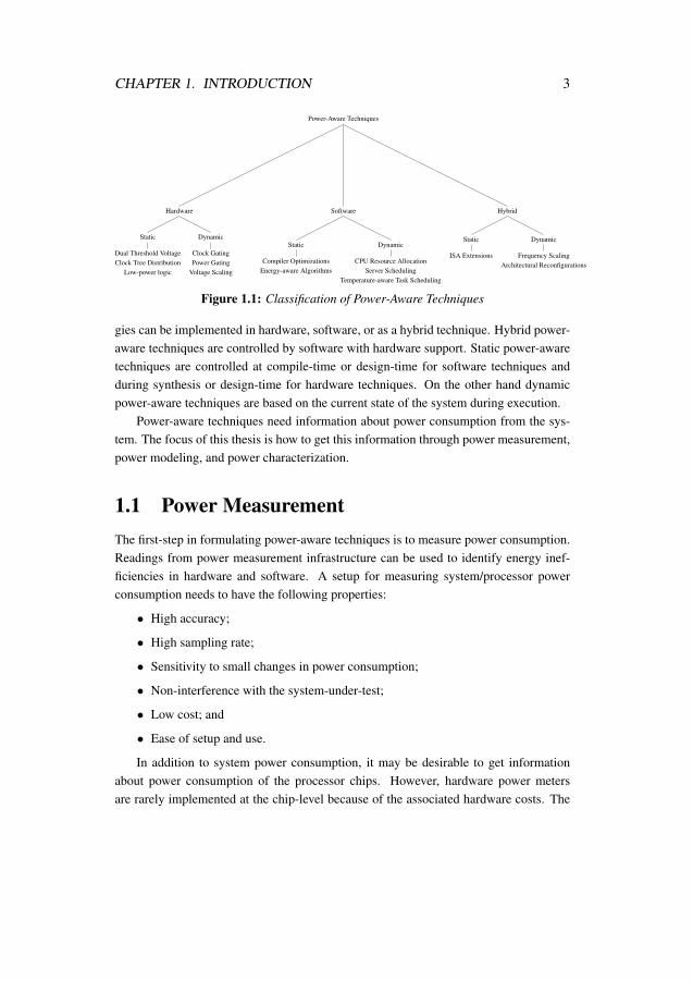
We classify power-aware techniques as shown in Fig. 1.1. The power-aware strate-
2
CHAPTER 1. INTRODUCTION 3
Power-Aware Techniques
Hardware
Static
Dual Threshold VoltageClock Tree Distribution
Low-power logic
Dynamic
Clock GatingPower Gating
Voltage Scaling
Software
Static
Compiler OptimizationsEnergy-aware Algorithms
Dynamic
CPU Resource AllocationServer Scheduling
Temperature-aware Task Scheduling
Hybrid
Static
ISA Extensions
Dynamic
Frequency ScalingArchitectural Reconfigurations
Figure 1.1: Classification of Power-Aware Techniques
gies can be implemented in hardware, software, or as a hybrid technique. Hybrid power-aware techniques are controlled by software with hardware support. Static power-awaretechniques are controlled at compile-time or design-time for software techniques andduring synthesis or design-time for hardware techniques. On the other hand dynamicpower-aware techniques are based on the current state of the system during execution.
Power-aware techniques need information about power consumption from the sys-tem. The focus of this thesis is how to get this information through power measurement,power modeling, and power characterization.
1.1 Power MeasurementThe first-step in formulating power-aware techniques is to measure power consumption.Readings from power measurement infrastructure can be used to identify energy inef-ficiencies in hardware and software. A setup for measuring system/processor powerconsumption needs to have the following properties:
• High accuracy;
• High sampling rate;
• Sensitivity to small changes in power consumption;
• Non-interference with the system-under-test;
• Low cost; and
• Ease of setup and use.
In addition to system power consumption, it may be desirable to get informationabout power consumption of the processor chips. However, hardware power metersare rarely implemented at the chip-level because of the associated hardware costs. The

CHAPTER 1. INTRODUCTION 4
power consumption of the system can be measured in multiple ways. We compare dif-ferent approaches to measuring the power consumption and discuss advantages and dis-advantages of each.
1.2 Power ModelingDepending on the requirements and costs, it may not be possible to use actual powermeasurements. For example, it may be too costly to deploy the power measurementsetup at multiple machines, or the response time of the power measurement setup maynot be fast enough for a particular power-aware technique. An alternative to actual powermeasurement is to estimate the power consumption using models that provide powerestimates based on events in the system. They can be implemented in either hardware orsoftware. Power models should have following properties:
• Small delay between input and output;
• Low overhead — low CPU usage if software model and low hardware area ifhardware model;
• High accuracy; and
• Power consumption information of individual components (like cores or microar-chitectural components).
Based on the requirements of the power-aware technique and trade-offs among costs,accuracy, and overhead, the system designer must decide whether to implement hard-ware or software power model. Intel introduced a hardware power model in its Core i7processors starting with the Sandy Bridge microarchitecture [6]. The values from thispower model are available to the software using Model Specific Registers (MSR) throughthe Running Average Power Limit (RAPL) interface. Similar model-based power esti-mates are available for AMD processors through their Application Power Management(APM) Interface [7], and on NVIDIA GPU processors through NVIDIA ManagementLibrary (NVML) [8]. In addition to these relatively new power models implementedin hardware by chip manufacturers, researchers have proposed software power mod-els [9–18].
The information gained by power metering and power modeling can be used byresource management software to make power-aware decisions. Research studies havemade use of live power measurement to schedule tasks and allocate resources at the levelof individual processors [11,19,20,20–23] and large data centers [15,24–29]. Power/en-ergy models have been used in many research studies to propose power-aware strategiesfor controlling DVFS policies [19, 23], task scheduling in chip multiprocessors [24] and

CHAPTER 1. INTRODUCTION 5
data centers [27,28], power budgeting [11,21], energy-aware accounting and billing [30],and avoiding thermal hotpsots in chip multiprocessors [31, 32].
In this thesis, we develop a performance event and temperature based per-core powermodel for chip multiprocessors. Our model estimates power in real time with low over-head.
1.3 Power CharacterizationPower characterization analyzes the system’s energy expenditure for varying workloads. This can be used to devise software and hybrid power-aware strategies, optimize work-loads for energy efficiency, and optimize system design. Some of the challenges forenergy characterization are:
• Choosing representative workloads. Workloads selected for characterizationstudies should be representative of those that are likely to be run on the system.The workloads should also exercise the full spectrum of identified system char-acteristics for extensive analysis.
• Choosing good metrics. The selection of the metrics to characterize and comparesystem energy expenditure depends on the type of characterization study and theemphasis that the researchers wants to put on delay versus energy expenditure.Possible metrics include total energy, average power, peak power, dynamic power,energy-delay product, energy-delay-squared product, and power density.
• Setting up appropriate power metering infrastructure. Any energy character-ization study requires a means to measure/estimate and log system power con-sumption. Depending on the type of study, measurement factors like accuracyand temporal granularity must be considered. It may be useful to be able to de-compose power consumption figures for different system components but thatsupport may or may not exist. Researchers need to consider these factors anddecide between measuring actual power versus modeling the power estimates.
Researchers have used energy characterization to understand energy-efficiency ofmobile platforms [33–35] and desktop/server platforms [15, 36–38]. Energy charac-terization can also be used to analyze the energy efficiency of specific features of thesystem [39, 40]. The energy behaviors thus characterized can be used, for example, toidentify software inefficiencies [33, 34, 36], manage power [15], analyze power/perfor-mance trade-offs [41], and compare energy efficiency of competing technologies [39].Apart from actual power measurement, power models can prove to be useful for energycharacterization [39, 41, 42].

CHAPTER 1. INTRODUCTION 6
In this thesis, we characterize performance and energy of Intel’s recent Haswellmicroarchitecture with a focus on its support for transactional memory.
1.4 Thesis OrganizationThe rest of this thesis is organized as follows:
• In Chapter 2, we explain different techniques to measure power consumptionof the system, compare their intrusiveness, and give experimental results to showtheir accuracy and sensitivity. We test Intel’s hardware power model for accuracy,sensitivity, and update granularity and discuss the results.
• In Chapter 3, we present a per-core, portable, scalable power model and showthe validation results across multiple platforms. We show the effectiveness ofthe model by implementing it in an experimental meta-scheduler power-awarescheduling.
• In Chapter 4, we present performance and energy expenditure characterizationresults for Restricted Transactional Memory (RTM) implementation on the IntelHaswell microarchitecture. We use microbenchmarks and the STAMP bench-mark suite to compare the performance and energy efficiency of RTM to TinySTM— a software transactional memory implementation.
• In Chapter 5 we present our concluding remarks and discuss future researchdirections that can be taken from the work presented in this thesis.

2Power Measurement Techniques
2.1 OverviewDesigning intelligent power-aware computing technologies requires an infrastructurethat can accurately measure and log the system power consumption and preferably that ofthe system’s individual resources. Resource managers can use this information to iden-tify power consumption problems in both hardware (e.g., hotspots) and software (e.g.,power-hungry tasks) and then to address those problems (e.g., through scheduling tasksto even out power or temperature across the chip) [12,43,44]. A measurement infrastruc-ture can also be used for power benchmarking [45, 46], power modeling [12, 13, 15, 43]and power characterization [36,47,48]. In this chapter, we compare different approachesto measuring actual power consumption on the Intel CoreTM i7 platform. We discussthese techniques in terms of their intrusiveness, ease of use, accuracy, timing resolution,sensitivity, and overhead. The measurement techniques demonstrated in this chapter canbe applied to other platforms, subject to some hardware support.
In the absence of techniques to measure actual power consumption, model-basedpower consumption estimation is also a viable alternative. Intel’s Running AveragePower Limit (RAPL) interface [6], AMD’s Application Power Management (APM) in-
7

CHAPTER 2. POWER MEASUREMENT TECHNIQUES 8
CPU
1 2
3
Data Logging
Machine
Power Supply
UnitWatts? Up
PRO
Custom
Sense
Hardware
Data Acquisition
Device
Buck
Controller
Wall
Outlet
Machine Under TestMotherboard
+5V
+3.3V+12V1/2+12V3
AC AC
Figure 2.1: Power Measurement Setup
terface [7] and NVIDIA’s Management Library (NVML) [8] interface make model-basedenergy estimates available to the operating system and user applications through model-specific registers, thereby enabling the software to make power-aware decisions.
In the rest of this chapter, we first describe the methodology of three techniquesto measure actual power consumption, discuss their advantages and disadvantages, andcollect experimental results on an Intel CoreTMi7 870 platform to compare their accuracyand sensitivity. We then compare one of these measurement techniques — reading powermeasurement from the ATX (Advanced Technology eXtended) power rails — to Intel’sRAPL implementation on CoreTMi7 4770 (Haswell).
2.2 Power Measurement TechniquesPower consumption can be measured at various points in a system. We measure powerconsumption at three points, as shown in Fig. 2.1:
1. The first and least intrusive method for measuring the power of an entire systemis to use a power meter like the Watts up? Pro [49] plugged directly into the walloutlet;
2. The second method uses custom sense hardware to measure the current on indi-vidual ATX power rails; and
3. The third and most intrusive method measures the voltage and current directly atthe CPU voltage regulator.
2.2.1 At the Wall OutletThe first method uses an off-the-shelf (Watts up? Pro) power meter that sits between thesystem under test and the power outlet. Note that to prevent data logging activity fromdisturbing the system under test, we use a separate machine to collect measurements forall three techniques, as shown in Fig. 2.1. Although easy to deploy and non-intrusive,

CHAPTER 2. POWER MEASUREMENT TECHNIQUES 9
this meter delivers only a single system measurement, making it difficult to separate thepower consumption of different system components. Moreover, the measured powervalues are inflated compared to actual power consumption due to inefficiencies in thesystem power supply unit (PSU) and on-board voltage regulators. The acuity of themeasurements is also limited by the (low) sampling frequency of the power meter: onesample per second (here on referred to as Sa/s) for the Watts up? Pro. The accuracyof the system power readings depends on the accuracy specifications provided by themanufacturer (±1.5% in our case). The overall accuracy of measurements at the walloutlet is affected by the mechanism converting between alternating current (AC) to directcurrent (DC) in the power supply unit. When we discuss measurement results below, weexamine the accuracy effects of the AC-DC conversion done by the PSU.
This approach is suitable for studies of total system power consumption instead ofindividual components like the CPU, memory, or graphics cards [50,51]. It is also usefulin power modeling research, where the absolute value of the CPU and/or memory powerconsumption is less important than the trends [43].
2.2.2 At the ATX Power RailsThe second methodology measures current on the supply rails of the ATX motherboard’spower supply connectors. As per the ATX power supply design specifications [52], thepower supply unit delivers power to the motherboard through two connectors, a 24-pinconnector that delivers +5.5V, +3.3V, and +12V, and an 8-pin connector that delivers+12V used exclusively by the CPU. Table 2.1 shows the pinouts of these connectors.Depending on the system under test, the pins belonging to the same power region maybe connected together on the motherboard. In our case, all +3.3 VDC pins are connectedtogether, as are all +5 VDC pins and +12V3 pins. Apart from that, the +12V1 and +12V2pins are connected together to supply current to the CPU. Hence, to measure the totalpower consumption of the motherboard, we can treat these connections as four logicallydistinct power rails — +3.3V, +5V, +12V3, and +12V1/2.
For our experiments, we develop custom measurement hardware using current trans-ducers from LEM [53]. These transducers use the Hall effect to generate an outputvoltage in accordance with the changing current flow. The top-level schematic of thehardware is shown in Fig. 2.2, and Fig. 2.3 shows the manufactured board. Note thatwhen designing such a printed circuit board (PCB), care must be taken to ensure thatthe current capacity of the PCB traces carrying the combined current for the ATX powerrails is sufficiently high and that the on-board resistance is as low as possible. We use aPCB with 105 micron copper instead of the more widely used thickness of 35 microns.Traces carrying high current are at least 1 cm wide and are backed by thick-stranded wire

CHAPTER 2. POWER MEASUREMENT TECHNIQUES 10
(a) 24-pin ATX Connector Pinout
Pin Signal Pin Signal
1 +3.3 VDC 13 +3.3 VDC2 +3.3 VDC 14 -12 VDC3 COM 15 COM4 +5 VDC 16 PS_ON5 COM 17 COM6 +5 VDC 18 COM7 COM 19 COM8 PWR OK 20 Reserved9 5 VSB 21 +5 VDC
10 +12 V3 22 +5 VDC11 +12 V3 23 +5 VDC12 +3.3 VDC 24 COM
(b) 8-pin ATX ConnectorPinout
Pin Signal Pin Signal
1 COM 5 +12 V12 COM 6 +12 V13 COM 7 +12 V24 COM 8 +12 V2
Table 2.1: ATX Connector Pinout
connections, when required. The current transducers need +5V supply voltage, which isprovided by the +5VSB (stand by) rail from the ATX connector. Using +5VSB for thetransducer’s supply serves two purposes. First, because the +5VSB voltage is availableeven when the machine is powered off, we can measure the base output voltage from thecurrent transducers for calibration purposes. Second, because the current consumed bythe transducers themselves (∼28mA) is drawn from +5VSB, it does not interfere withour power measurements. We sample and log the analog voltage output from the currenttransducers using a data acquisition (DAQ) unit from National Instruments (NI USB-6210 [54]).
As per the LEM datasheet, the base voltage of the current transducer is 2.5V. Ourexperiments indicate that the current transducer produces an output voltage of 2.494Vwhen zero current is passed through its primary turns. The sensitivity of the currenttransducer is 25mV/A, hence the current can be calculated as in Eq. 2.1.
Iout =Vout −BASE_V OLTAGE
0.025(2.1)
We verify our current measurements by comparing against the output from a digi-tal multimeter. The power consumption can then be calculated by simply multiplyingthe current with the respective voltage. Apart from the ATX power rails, the PSU alsoprovides separate power connections to the hard drive, CD-ROM, and cabinet fan. Tocalculate the total PSU load without adding extra hardware, we disconnect the I/O de-

CHAPTER 2. POWER MEASUREMENT TECHNIQUES 11
3.3V LTS25-NP
PSU
24-P
in8
-Pin
MB
24-P
in8
-Pin
NI USB-6210
5V
12V
12V
PCB
LTS25-NP
LTS25-NP
LTS25-NP
LTS25-NP
LTS25-NP
Figure 2.2: Measurement Setup on the ATX Power Rails
vices and fan, and we boot our system from a USB memory device powered by themotherboard. The total power consumption of the motherboard can then be calculatedas in Eq. 2.2.
P = I3.3V ∗ V3.3V + I12V 3 ∗ V12V 3 + I5V ∗ V5V + I12V 1/2 ∗ V12V 1/2 (2.2)
The theoretical current sensitivity of this measurement infrastructure can be calcu-lated by dividing the voltage sensitivity of the DAQ unit (47µV) by the current sensitivityof the LTS-25NP current transducers from LEM (25mV/A). This yields a current sensi-tivity of 2mA.
This approach improves accuracy by eliminating the complexity of measuring ACpower. Furthermore, the approach enjoys greater sensitivity to current changes (2mA)and higher acquisition unit sampling frequencies (up to 250000 Sa/s). Since most mod-ern motherboards have separate supply connectors for the CPU(s), this approach facil-itates distinguishing CPU power consumption from that of other motherboard compo-nents. Again, this improvement comes with increased cost and complexity: the sophis-ticated DAQ unit is priced an order of magnitude higher than the power meter, and wehad to build a custom board to house the current transducer infrastructure.
2.2.3 At the Processor Voltage RegulatorAlthough measurements taken at the motherboard supply rails factor out the power sup-ply unit’s efficiency curve, they are still affected by the efficiency curve of the on-boardvoltage regulators. To eliminate this source of inaccuracy, we investigate a third ap-proach. Motherboards that follow Intel’s processor power delivery guidelines (VoltageRegulator-Down (VRD) 11.1 [55]) provide a load indicator output (IMON/Iout) from

CHAPTER 2. POWER MEASUREMENT TECHNIQUES 12
Motherboard
Connection
LTS-25NP
To
USB-6210
PSU
Connection
Figure 2.3: Our Custom Measurement Board
the processor voltage regulator. This load indicator is connected to the processor for useby the processor’s power management features. This signal provides an analog voltagelinearly proportional to the total load current of the processor. We use this current sens-ing pin from the processor’s voltage regulator chip (CHL8316, in our case) to acquirereal-time information about total current delivered to the processor. We also use thevoltage output at the V_CPU pin of the voltage regulator, which is directly connectedto the CPU voltage supply input of the processor. We locate these two signals on themotherboard and solder wires at the respective connection points (the resistor/capacitorpads connected to these signals). We connect these two signals and the ground pointto our DAQ unit, logging the values read on the separate test machine. This currentmeasurement setup is shown in Fig. 2.4.
The full voltage swing of the IMON output is 900mV for the full-scale current of140A (for the motherboard under test). Hence, the current sensitivity of the IMON out-put comes to about 6.42mV/A. The theoretical sensitivity of this infrastructure dependson the voltage sensitivity of the DAQ unit (47µV) and its overall sensitivity to currentchanges comes to 7mA. This sensitivity is less than that for measuring current at theATX power rails, but the sensitivity may vary for different voltage regulators on differ-ent motherboards. This method provides the most accurate measurements of absolutecurrent feeding the processor, but it is also the most intrusive, as it requires solderingwires on the motherboard, an invasive instrumentation procedure that should only beperformed by skilled technicians. Moreover, these power measurements are limited toprocessor power consumption (we get no information about other system components).For example, for memory-intensive applications, we can account for power consumption

CHAPTER 2. POWER MEASUREMENT TECHNIQUES 13
Figure 2.4: Measurement Setup on CPU Voltage Regulator
effects of the external bus transactions triggered by off-chip memory accesses, but thismethod provides no means of measuring power consumed in the DRAMs. The accuracyof the IMON output is specified by the CHL8316 datasheet to be within ±7%. This fallsfar below the 0.7% accuracy of the current transducers at the ATX power rails1.
2.2.4 Experimental ResultsWe use an Intel CoreTMi7 870 processor to compare power measurement readings at thewall outlet, at the ATX power rails, and directly on the processor’s voltage regulator.
The Watts Up? Pro measures power consumption of the entire system at the rate of1 Sa/s, whereas the data acquisition unit is configured to capture samples at the rate of40000 Sa/s from the four effective ATX voltage rails (+12V1/2, +12V3, +5V and +3.3V)and the V_CPU and the IMON outputs of the CPU voltage regulator. We choose this ratebecause the combined sampling rate of the six channels adds up to 240K Sa/s, and themaximum sampling rate supported by the DAQ is 250K Sa/s. To remove background
1The accuracy specifications of the processor’s voltage regulator may differ for different manu-facturers.
CHAPTER 2. POWER MEASUREMENT TECHNIQUES 14
0 10000 20000 30000 40000 50000Time (msec)
0
50
100
Pow
er (W
)
Outlet PowerMB CPU PowerATX CPU Power
CPU Idle1 core
2 cores
4 cores
3 cores
Figure 2.5: Power Measurement Comparison When Varying the Number of Active Cores
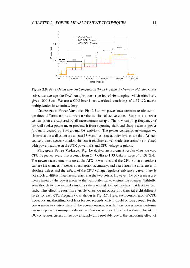
noise, we average the DAQ samples over a period of 40 samples, which effectivelygives 1000 Sa/s. We use a CPU-bound test workload consisting of a 32×32 matrixmultiplication in an infinite loop.
Coarse-grain Power Variance. Fig. 2.5 shows power measurement results acrossthe three different points as we vary the number of active cores. Steps in the powerconsumption are captured by all measurement setups. The low sampling frequency ofthe wall-socket power meter prevents it from capturing short and sharp peaks in power(probably caused by background OS activity). The power consumption changes weobserve at the wall outlet are at least 13 watts from one activity level to another. At suchcoarse-grained power variation, the power readings at wall outlet are strongly correlatedwith power readings at the ATX power rails and CPU voltage regulator.
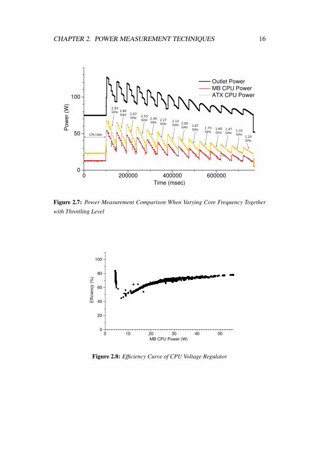
Fine-grain Power Variance. Fig. 2.6 depicts measurement results when we varyCPU frequency every five seconds from 2.93 GHz to 1.33 GHz in steps of 0.133 GHz.The power measurement setup at the ATX power rails and the CPU voltage regulatorcapture the changes in power consumption accurately, and apart from the differences inabsolute values and the effects of the CPU voltage regulator efficiency curve, there isnot much to differentiate measurements at the two points. However, the power measure-ments taken by the power meter at the wall outlet fail to capture the changes faithfully,even though its one-second sampling rate is enough to capture steps that last five sec-onds. This effect is even more visible when we introduce throttling (at eight differentlevels for each CPU frequency), as shown in Fig. 2.7. Here, each combination of CPUfrequency and throttling level lasts for two seconds, which should be long enough for thepower meter to capture steps in the power consumption. But the power meter performsworse as power consumption decreases. We suspect that this effect is due to the AC toDC conversion circuit of the power supply unit, probably due to the smoothing effect of

CHAPTER 2. POWER MEASUREMENT TECHNIQUES 15
0 20000 40000 60000 80000 100000Time (msec)
0
50
100
Pow
er (W
)Outlet PowerMB CPU PowerATX CPU Power
CPU Idle
2.93GHz 2.80
GHz2.67GHz 2.53
GHz 2.40GHz
2.27GHz
2.13GHz 2.00
GHz1.87GHz
1.73GHz
1.60GHz
1.47GHz
1.33GHz
Figure 2.6: Power Measurement Comparison When Varying Core Frequency
the capacitor in the PSU. These effects are not visible between measurement points atthe ATX power rails and CPU voltage regulator.
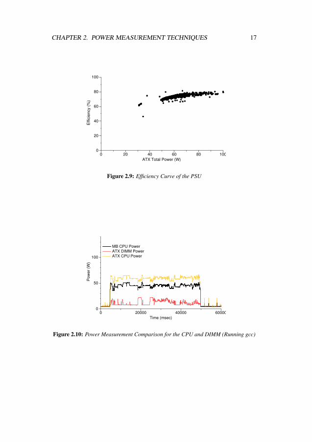
Fig. 2.8 shows the efficiency curve of the CPU voltage regulator at various loadlevels. The voltage regulator on the test system employs dynamic phase control to adjustthe number of phases with varying load current to try to optimize the efficiency over awide range of loads. The voltage regulator switches to one-phase or two-phase operationto increase the efficiency at light loads. When the load increases, the regulator switchesto four-phase operation at medium loads and six-phase operation at high loads. Thesharp change in efficiency visible in Fig. 2.8 is likely due to adaptation in phase control.Fig. 2.9 shows the obtained efficiency curve of the cabinet PSU against total powerconsumption calculated on the ATX power rails. The total system power never goesbelow 30W, and the efficiency of the PSU varies from 60% to around 80% in the outputpower range from 30W to 100W.
Fig. 2.10 shows the changes in CPU and main memory power consumption whilerunning gcc from SPEC CPU2006. Power consumption of the main memory varies fromaround 7.5W to 22W across various phases of the gcc run. Researchers and practitionerswho wish to assess main memory power consumption will at least want to measurepower at the ATX power rails.
CHAPTER 2. POWER MEASUREMENT TECHNIQUES 16
0 200000 400000 600000Time (msec)
0
50
100
Pow
er(W
)
Outlet PowerMB CPU PowerATX CPU Power
CPU Idle
2.93GHz 2.80
GHz 2.67GHz 2.53
GHz 2.40GHz
2.27GHz
2.13GHz 2.00
GHz 1.87GHz 1.73
GHz1.60GHz
1.47GHz
1.33GHz
1.20GHz
Figure 2.7: Power Measurement Comparison When Varying Core Frequency Together
with Throttling Level
0 10 20 30 40 50
MB CPU Power (W)
0
20
40
60
80
100
E
ffic
iency (
%)
Figure 2.8: Efficiency Curve of CPU Voltage Regulator
CHAPTER 2. POWER MEASUREMENT TECHNIQUES 17
0 20 40 60 80 100
ATX Total Power (W)
0
20
40
60
80
100
E
ffic
ien
cy (
%)
Figure 2.9: Efficiency Curve of the PSU
0 20000 40000 60000
Time (msec)
0
50
100
P
ow
er
(W)
MB CPU Power
ATX DIMM Power
ATX CPU Power
Figure 2.10: Power Measurement Comparison for the CPU and DIMM (Running gcc)
CHAPTER 2. POWER MEASUREMENT TECHNIQUES 18
2.3 RAPL power estimations
2.3.1 OverviewIntel introduced Running Average Power Limit (RAPL) interface on the Sandy Bridgemicroarchitecture. The programmers can use the RAPL interface for enforcing powerconsumption constraint on the processor. This interface includes non-architectural Model-specific registers (MSRs) for setting the power limit and reading the energy consumptionstatus of the processor power domains like processor die and DRAM2. The energy con-sumption information provided by the RAPL interface is not based on actual currentmeasurement from physical sensors, but a power model based on performance eventsand probably other inputs like temperature, voltage, etc. As per Intel specifications, theRAPL energy status counter is updated approximately every 1ms, giving a maximumsampling frequency of 1000 Sa/s. Since Intel has not specified the details of the powermodel, the only way to measure the accuracy of the model is through experimentation.In the following sections, we compare power measurement readings from RAPL and theATX power rails.
2.3.2 Experimental ResultsWe use Intel CoreTMi7 4770 processor to compare power measurement results at theATX power rails and Intel’s RAPL energy counter. For reading the RAPL energycounter, we use the x86-MSR driver to read the RAPL energy counter MSR calledMSR\_PKG\_ENERGY\_STATUS. We set up a real-time timer that raises SIGALRM atconfigured intervals to read the MSR. The ATX power measurement infrastructure is thesame as described for Intel CoreTMi7 870 processor. Below we describe our experimentsto validate the RAPL energy counter readings.
RAPL Overhead. One of the major differences between measuring power usingRAPL and other techniques shown in Figure 2.1 is that the RAPL measurements aredone on the same machine that is being tested. As a result, reading the RAPL energycounter at frequent intervals adds some overhead to the system power. To test this,we run our RAPL counter reading tool at the sampling frequency of 1 Sa/s, 10 Sa/sand 1000 Sa/s and monitor the change in system power consumption on the ATX CPUpower rails. The results from this experiment are shown in Fig. 2.11. The spikes inpower consumption visible in the figure indicate the starting of the RAPL reading utility.These spikes mainly result from loading dynamic libraries and can be ignored, assum-ing that the RAPL utility is started before running any benchmark under test. These
2The DRAM energy status counter is only available on server platforms.

CHAPTER 2. POWER MEASUREMENT TECHNIQUES 19
0 10000 20000 30000
Time (msec)
0
5
10
15
Pow
er
(W)
1000 S/s10 S/s1 S/s
Figure 2.11: Power Overhead Incurred While Reading the RAPL Energy Counter
spikes however act as useful synchronization points to overlap readings from RAPL andthe ATX power rails. For calculating the RAPL power overhead, we concentrate on theCPU power consumption after the initial power spike. As seen from the figure, readingthe RAPL MSR every second and every 100ms adds no discernible power consump-tion to the idle system power, but reading the RAPL counter every 1ms adds 0.1W ofpower overhead. However, this small power overhead comes mainly from generatingSIGALRM every millisecond and not from reading the MSR. Hence, if the reading ofRAPL energy counter is done as part of the existing software infrastructure like a kernelscheduler, this will not add discernible overhead to CPU power consumption.
RAPL Resolution. As per the Intel specification manual [56], the RAPL energycounter is updated about every 1ms. To test this update frequency, we run the matrixmultiplication application described in Section 2.2.4 while reading the RAPL energystatus counter every 1ms. We sample the ATX power rails every 10µS and average over100 samples. The results from this experiment are shown in Fig. 2.12. Although theRAPL readings follow the same curve as those from the ATX power rails, two thingsare of note here. First, the RAPL readings show more deviation from the mean than theATX readings. Second, there are huge deviations from the mean at periodic intervalsof around 1.6-1.7 seconds. Hähnel et al. [48] observe that the RAPL counter is notupdated exactly at 1ms. As per their experiments, there can be a deviation of a few tensof thousands of cycles in the periodic interval at which the RAPL counter is updated ona given platform. This explains the small deviations from the mean we see in our RAPLreadings. They also observe that when the CPU switches to System Management Mode(SMM), the RAPL update is delayed until after the CPU comes out of SMM mode.This results in the RAPL energy counter showing no increment between two successive

CHAPTER 2. POWER MEASUREMENT TECHNIQUES 20
2 4 6 8 10 12 14 16 18 20
Time (sec)
0
20
40
60
80
P
ow
er
(W)
RAPL Power
ATX CPU Power
Figure 2.12: Power Measurement Comparison for the ATX and RAPL at the RAPL
Sampling Rate of 1000 Sa/s
readings, creating a negative deviation. The next update to the counter increments theenergy value expended by the processor in last 2ms instead of 1ms, creating a positivedeviation. On our system, the CPU switches to SMM every 1.6-1.7 seconds, whichcauses inaccurate energy readings.
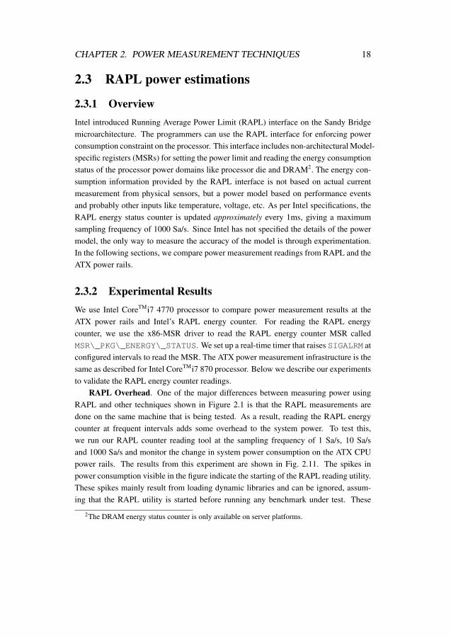
RAPL Accuracy. To test the accuracy of the RAPL readings, we first repeat theDVFS test from Fig. 2.6 in Section 2.2.4 and take the power measurement readingsfrom the ATX power rail and RAPL. Each DVFS operating point is maintained for fiveseconds. The ATX power is sampled at 10000 Sa/s while the RAPL counter is sampledat 10 Sa/s. The results from this test are shown in Fig. 2.13. The RAPL measurementcurve follows the ATX measurement curve faithfully, although their y-axis scales arenecessarily different. This test shows that the RAPL model works well across differentDVFS frequencies.
Next, we simulate a real-time application in which a task is started at fixed periodicintervals. We compare power measurement from RAPL and ATX while varying the taskperiod. We set up a timer to raise SIGALRM signal, and a matrix multiplication task isstarted at every timer interrupt. The matrix multiplication loop is configured to occupyabout 66% of the time period. We run this experiment for three different periods: 100ms,10ms, and 1ms. We gather samples between two consecutive SMM switches. We readthe RAPL counter every 1ms. We sample the ATX power rails every 5µS and averageover 20 samples. The results from this experiment are shown in Fig. 2.14. For the100ms and 10ms period, the RAPL readings closely follow the ATX readings, althoughthey are off by 1ms when the power consumption changes suddenly. As expected, for the1ms period test, RAPL is unable to capture the power consumption curve but accuratelyestimates the average power consumption.
CHAPTER 2. POWER MEASUREMENT TECHNIQUES 21
20 40 60 80 100
Time (sec)
0
10
20
30
40
50
P
ow
er
(W)
RAPL Power
ATX CPU Power
Figure 2.13: Power Measurement Comparison for ATX and RAPL When Varying Core
Frequency
Since the RAPL energy counter values are based on a performance event basedpower model [6], we also test the RAPL accuracy using a microbenchmark that runsinteger operations, floating-point operations and memory operations in different phases.For this experiment, we sample the RAPL energy counter at 100Sa/S. We sample theATX CPU power rails at 10000 Sa/s and then average over 100 samples. We also samplethe ATX 5V power rails, which on our system mainly supplies the DRAM memory.The results are shown in Fig. 2.15. The deviations that we see in Fig. 2.12 due to CPUswitching to SMM are visible in this Fig. 2.15 as well. Because we sample the RAPLcounter every 10ms instead of 1ms, we only see 10% deviation from the mean insteadof 100%. Apart from these deviations that occur every 1.7 second (effectively one outof 170 samples), the RAPL energy readings are accurate for all of the integer, floating-point and memory-intensive phases. To quantify the RAPL power estimation accuracy,we calculate Spearman’s rank correlation coefficient for RAPL and ATX CPU readingsfor the microbenchmark run. The correlation coefficient is ρ=0.9858. In comparison,the correlation coefficient between the ATX CPU power and motherboard CPU powershown in Fig. 2.7 is ρ=0.9961. Sample values from the ATX show that DRAM poweris significant, which is not captured by the RAPL package energy counter. Power-awarecomputing methodologies must take this into consideration. The RAPL interfaces onIntel processors for server platforms include an energy counter for the DRAM domaincalled MSR\_DRAM\_ENERGY\_STATUS. This can be useful for assessing the powerconsumption of the DRAM memory.
Based upon our experimental results, we conclude that the RAPL energy counteris good for estimating energy for a duration of more than 1ms. However, when theresearcher is interested in instantaneous power trends, especially peak power trends,

CHAPTER 2. POWER MEASUREMENT TECHNIQUES 22
100 200 300 400
Time (msec)
0
5
10
15
20
P
ow
er
(W)
RAPL Power
ATX CPU Power
(a) 100ms period test
10 20 30 40
Time (msec)
0
5
10
15
20
P
ow
er
(W)
RAPL Power
ATX CPU Power
(b) 10ms period test
1 2 3 4
Time (msec)
0
5
10
15
20
P
ow
er
(W)
RAPL Power
ATX CPU Power
(c) 1ms period test
Figure 2.14: Power Measurement Comparison for ATX and RAPL with Varying Real-
time Application Period

CHAPTER 2. POWER MEASUREMENT TECHNIQUES 23
200 400 600 800
Time (sec)
0
20
40
60
P
ow
er
(W)
RAPL Power
ATX CPU Power
ATX DIMM Power
Figure 2.15: Accuracy Test of RAPL for Custom Microbenchmark
sampling the actual power consumption using an accurate measurement infrastructure(like ours) is a better choice.
2.4 Related WorkHackenberg et al. [57] compare several measurement techniques for signal quality, ac-curacy, timing resolution, and overhead. They use both Intel and AMD systems in theirstudy. Their experimental results complement our results. There have been many inter-esting studies on power-modeling and power-aware resource management. These em-ploy various means to measure empirical power. Rajamani et al. [11] use on-board senseresistors located between the processor and voltage regulators to measure power con-sumed by the processor. They use a National Instruments isolation amplifier and data ac-quisition unit to filter, amplify, and digitize their measurements. Isci and Martonosi [58]measure current on the 12V ATX power lines using clamp ammeters, that are hookedto a digital multimeter (DMM) for data collection. The DMM is connected to a datalogging machine via an RS232 serial port. Contreras and Martonosi [14] use jumperson their Intel XScaleTM development board to measure the power consumption of theCPU and memory separately. They feed the measurements to a LeCroy oscilloscope forsampling. Cui et al. [59] also measure the power consumption at the ATX power rails.They use current-sense resistors and amplifiers to generate sense voltages (instead ofusing current transducers), and they log their measurements using a digital multimeter.Bedard et al. [51] build their own hardware that combines the voltage and current mea-surements and host interface into one solution. They use an Analog Devices ADM1191digital power monitor to sense voltage and current values and an Atmel R© microcon-

CHAPTER 2. POWER MEASUREMENT TECHNIQUES 24
troller to send the measured values to a host USB port. Hähnel et al. [48] experimentwith the update granularity of the RAPL interface and report practical considerations forusing the RAPL energy counter for power measurement. We find their results useful inexplaining our experiments.
2.5 ConclusionIn this chapter, we demonstrate different techniques that can be employed to measurepower consumption of the full system, CPU and DRAM memory. We compare the dif-ferent techniques in terms of accuracy, level sensitivity and temporal granularity anddiscuss their advantages and disadvantages. We test Intel’s RAPL energy counter resultsfor overhead, accuracy, and update granularity. We conclude that the RAPL counter forreading package energy incurs almost no power overhead and is fairly accurate for esti-mating energy over periods of more than few tens of milliseconds. However, because ofirregularities in the frequency at which the RAPL counter is updated, it shows deviationsfrom the average power when it is sampled at a faster rate.

3Per-core Power Estimation Model
3.1 OverviewPower measurement techniques described in Chapter 2 are essential for analyzing thepower consumption of systems under test. However, these measurement techniques donot provide detailed information on the power consumption of individual processor coresor microarchitectural units (e.g., caches, floating point units, integer execution units). Todevelop resource-management mechanisms for an individual processor, system design-ers need to analyze power consumption at the granularity of processor cores or eventhe components within a processor core. This information can be provided by placingon-die digital power meters, but that increases the chip’s hardware cost. Hence, supportfor such fine-grained digital power meters is limited by chip manufacturers. Even whenmeasurement facilities exist — e.g., the Intel CoreTMi7-870 [60] features per-core powermonitoring at the chip-level — they are rarely exposed to the user. Indeed, power sens-ing, actuation, and management support is more often implemented at the blade levelwith a separate computer monitoring output [61, 62].
An alternative to hardware support for fine-grained digital power meters is to es-timate the power consumption at the desired granularity using software power models.
25

CHAPTER 3. PER-CORE POWER ESTIMATION MODEL 26
Such models can identify various power-relevant events in the targeted microarchitectureand then track those events to generate a representative power consumption value. Wecan characterize software power estimation models by the following attributes:
• Portability. The model should be easy to port from one platform to another;
• Scalability. The model should be easy to scale across varying number of activecores and across different CPU voltage-frequency points;
• CPU Usage. The model’s CPU footprint should be negligible, so as not to pollutethe power consumption values of the system under test;
• Accuracy. The model’s estimated values should closely follow the empiricallymeasured power of the device that is modeled;
• Granularity. The model should provide power consumption estimates at thegranularity desired for the problem description (per core, per microarchitecturalmodule, etc.); and
• Speed. The model should supply power estimation values to the software at min-imal latency (preferably within microseconds).
In this thesis, we develop a power model that uses performance counters and temper-ature to generate accurate per-core power estimates in real time, with no off-line profilingor tracing. We build upon the power model developed by Singh et al. [16, 63] and in-clude some of their data for comparison. We validate their model on AMD K8 and IntelCoreTMi7 architectures. Below we explain our choice of using performance counters andtemperature to develop the model.
Performance Counters. We use performance counters for model formation be-cause the power models need a mechanism to track CPU activities with low overhead.Most modern processors are equipped with a Performance Monitoring Unit (PMU) pro-viding the ability to count the microarchitectural events of the processor. PMCs areavailable individually for each core and hence can be used to create core-specific mod-els. This allows programmers to analyze core performance, including the interactionbetween programs and the microarchitecture, in real time on real hardware, rather thanrelying on simplified and less accurate performance results from simulations. The PMUsprovide a wide variety of performance events. These events can be counted by mappingthem to a limited set of Performance Monitoring Counter (PMC) registers. For exam-ple, on Intel and AMD platforms, these performance counter registers are accessible asModel Specific Registers (MSRs). Also called Machine Specific Registers, these arenot necessarily compatible across processor families. Software can configure the perfor-mance counters to select which events to count. The PMCs can be used to count eventslike cache misses, micro-operations retired, stalls at various stages of an out-of-order

CHAPTER 3. PER-CORE POWER ESTIMATION MODEL 27
pipeline, floating point/memory/branch operations executed, and many more. Although,the counter values are not error-free [64,65] or even deterministic [66], if used correctly,the errors are small enough to make PMCs suitable candidates for estimating powerconsumption. The number and variety of performance monitoring events available formodern processors are increasing with each new architecture. For example, the numberof traceable performance events available in the Intel CoreTMi7-870 processor is aboutten times the number available in the Intel Core Duo processor [67]. This comprehensivecoverage of event information increases the probability that the available performancemonitoring events will be representative of overall microarchitectural activity for the pur-poses of performance and power analysis. This makes the use of performance countersto develop power models for hardware platforms very popular among researchers.
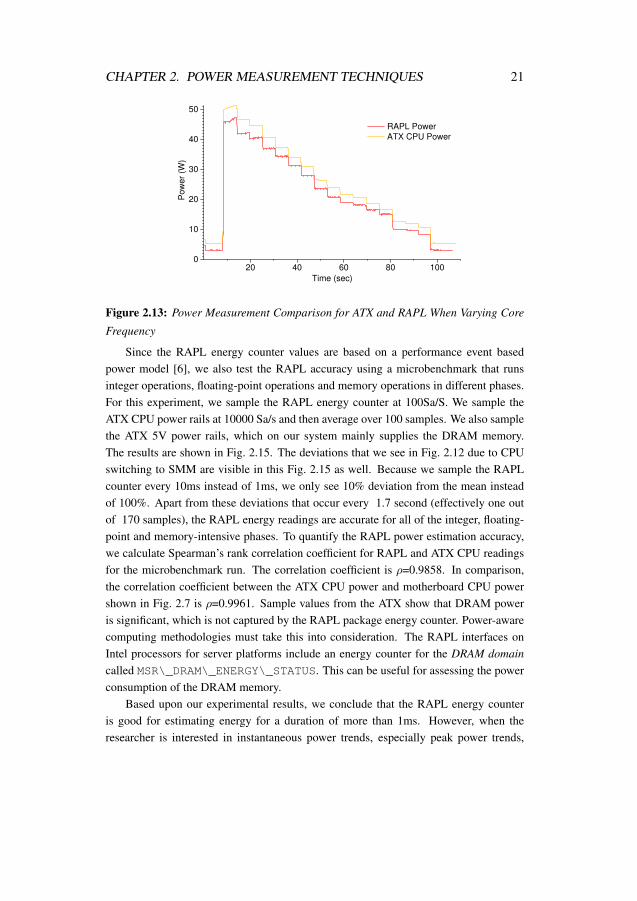
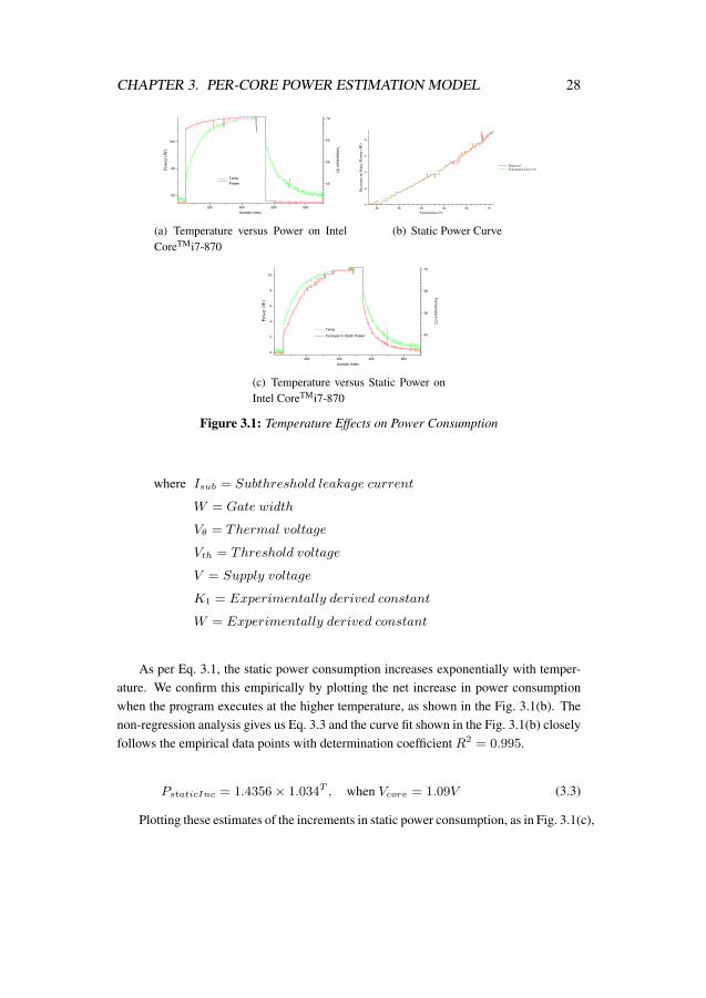
Temperature. Processor power consumption consists of both dynamic and staticelements. Among these, the static power consumption is dependent on the core temper-ature. Eq. 3.1 shows that the static power consumption of a processor is a function ofboth leakage current and supply voltage. The processor leakage current is a summationof subthreshold leakage and gate-oxide leakage current: Ileakage = Isub+Iox [68]. Thesubthreshold leakage current can be derived using Eq. 3.2 [68]. The Vθ component in theequation is thermal voltage, and it increases linearly with temperature. Since Vθ is in theexponents, subthreshold leakage current has an exponential dependence on temperature.With the increase in processor power consumption, processor temperature increases.This increase in temperature increases leakage current, which, in turn, increases staticpower consumption. To study the effects of temperature on power consumption, we rana multithreaded program executing MOV operations in a loop on our Intel CoreTMi7-870 machine. The rate of instructions retired, instructions executed, pipeline stalls andmemory operations remains constant over the entire run of the program. We also keepthe CPU operating frequency constant and observe that CPU voltage remains constantas well. This indicates that the dynamic power consumption of the processor does notchange over the run of the program. Fig. 3.1(a) shows that the total power consump-tion of the machine increases during the program’s runtime, and it coincides with theincrease in chip temperature. The total power consumption increases by almost 10%.To account for this increase in static power, it is necessary to include the temperature inpower models.
Pstatic =∑
Ileakage ∗ Vcore (3.1)
Isub = K1We−Vth/nVθ (1− e−V/Vθ ) (3.2)
CHAPTER 3. PER-CORE POWER ESTIMATION MODEL 28
200 400 600 800
Sample Index
60
80
100
Po
wer
(W)
Power 40
50
60
70
Te
mp
era
ture
(C)
Temp
(a) Temperature versus Power on IntelCoreTMi7-870
45 50 55 60 65 70
Temperature (C)
0
2
4
6
8
Incr
ease
in S
tati
c P
ow
er (
W)
Empirical
Exponential Curve Fit
(b) Static Power Curve
200 400 600 800
Sample Index
0
2
4
6
8
10
Po
wer
(W)
Increase in Static Power 40
50
60
70T
em
pe
ratu
re (C
)
Temp
(c) Temperature versus Static Power onIntel CoreTMi7-870
Figure 3.1: Temperature Effects on Power Consumption
where Isub = Subthreshold leakage current
W = Gate width
Vθ = Thermal voltage
Vth = Threshold voltage
V = Supply voltage
K1 = Experimentally derived constant
W = Experimentally derived constant
As per Eq. 3.1, the static power consumption increases exponentially with temper-ature. We confirm this empirically by plotting the net increase in power consumptionwhen the program executes at the higher temperature, as shown in the Fig. 3.1(b). Thenon-regression analysis gives us Eq. 3.3 and the curve fit shown in the Fig. 3.1(b) closelyfollows the empirical data points with determination coefficient R2 = 0.995.
PstaticInc = 1.4356× 1.034T , when Vcore = 1.09V (3.3)
Plotting these estimates of the increments in static power consumption, as in Fig. 3.1(c),
CHAPTER 3. PER-CORE POWER ESTIMATION MODEL 29
explains the gradual rise in total power consumption when the dynamic behavior of aprogram remains constant. Instead of using a non-linear function, we approximate thestatic power increase as a linear function of temperature. This is a fair approximationconsidering that the non-linear equation given in Eq. 3.3 can be closely approximatedwith the linear equation given in Eq. 3.4 with determination coefficient R2 = 0.989 (forthe range in which die temperature changes occur). This linear approximation avoids theadded cost of introducing an exponential term in the power model computation.
PstaticInc = 0.359× T − 16.566, when Vcore = 1.09V (3.4)
Modern processors allow programmers to read temperature information for eachcore from on-die thermal diodes. For example, Intel platforms report relative core tem-peratures on-die via Digital Thermal Sensors (DTS), which can be read by softwarethrough the MSRs or the Platform Environment Control Interface (PECI) [69]. Thisdata is used by the system to regulate CPU fan speed or to throttle the processor in caseof overheating. Third party tools like RealTemp and CoreTemp on Windows and open-source software like lm-sensors on Linux can be used to read data from the thermal sen-sors. As Intel documents indicate [69], the accuracy of temperature readings providedby the thermal sensors varies, and the values reported may not always match the actualcore temperatures. Because of factory variation and individual DTS calibration, readingaccuracy varies from chip to chip. The DTS equipment also suffers from slope errors,which means that temperature readings are more accurate near the T-junction max (themaximum temperature that cores can reach before thermal throttling is activated) thanat lower temperatures. DTS circuits are designed to be read over reasonable operatingtemperature ranges, and the readings may not show lower values than 20◦C even if theactual core temperature is lower. Since DTS is primarily created as a thermal protectionmechanism, reasonable accuracy at high temperatures is acceptable. This affects the ac-curacy of power models that use core temperature. Researchers and practitioners shouldread the processor model datasheet, design guidelines, and errata to understand the lim-itations of their respective thermal monitoring circuits, and they should take correctivemeasures when deriving their power models, if required.
3.2 Modeling ApproachOur approach to power modeling is workload-independent and does not require appli-cation modification. To show the effectiveness of our models, we perform two types ofstudies:
• We demonstrate accuracy and portability on five CMP platforms;

CHAPTER 3. PER-CORE POWER ESTIMATION MODEL 30
• We use the model in a power-aware scheduler to maintain a power budget
Studying sources of model error highlights the need for better hardware support forpower-aware resource management, such as fine-grained power sensors across the chipand more accurate temperature information. Our approach nonetheless shows promisefor balancing performance, power, and thermal requirements for platforms from embed-ded real-time systems to consolidated data centers, and even to supercomputers.
In the rest of the chapter, we first present the details of how we build our model,and then we discuss how we validate them. Our evaluation analyzes the model’s compu-tation overhead(Section 3.4.1) and accuracy(Section 3.4.2). We then explain the meta-scheduler that we use as a proof-of-concept for showing the effectiveness of our modelin Section 3.5.
3.3 Methodology
3.3.1 Counter SelectionSelecting appropriate PMCs to use is extremely important with respect to accuracy ofthe power model. We choose counters that are most highly correlated with measuredpower consumption. The chosen counters must also cover a sufficiently large set ofevents to ensure that they capture general application activity. If the chosen countersdo not meet these criteria, the model will be prone to error. The problem of choosingappropriate counters for power modeling has been handled in different ways by previousresearchers.
Research studies that estimate power for an entire core or a processor [11, 14, 15],use a small number of PMCs. Those that aim to construct decomposed power models toestimate the power consumption of sub-units of a core [10, 12, 13] tend to monitor morePMCs. The number of counters needed depends on the model granularity and the accept-able level of complexity. Also, most modern processors allow simultaneous counting ofonly a limited number (two/four/eight) microarchitectural events. Hence, using morecounters in the model requires interleaving the counting of events and extrapolating thecounter values over the total sampling period. This reduces the accuracy of absolutecounter values but allows researchers to track more counters.
To choose appropriate performance counters for developing our power-estimationmodel, we divide the available counters into four categories and then choose one counterfrom each category based upon statistical correlation [16,63]. This ensures that the cho-sen counters are comprehensive representations of the entire microarchitecture and arenot biased towards any particular section. Caches and floating point units form a largepart of the chip real estate, and thus PMCs that keep track of their activity factors would

CHAPTER 3. PER-CORE POWER ESTIMATION MODEL 31
be useful additions to the total power consumption information. Depending on the plat-form, multiple counters will be available in both these categories. For example, we cancount the total number of cache references as well as the number of cache misses for var-ious cache levels. For floating point operations, depending upon the processor model,we can count (separately or in combination) the number of multiplication, addition, anddivision operations. Because of the deep pipelining of modern processors, we can alsoexpect out-of-order logic to account for a significant amount of power. Stalls due tobranch mispredictions or an empty instruction decoder may reduce average power con-sumption over a fixed period of time. On the other hand, pipeline stalls caused by fullreservation stations and reorder buffers will be positively correlated with power becausethese indicate that the processor has extracted enough instruction-level parallelism tokeep the execution units busy. Hence, pipeline stalls indicate not just the power usageof out-of-order logic but of the executions units, as well. In addition, we would liketo use a counter that can cover all the microarchitectural components not covered bythe above three categories. This includes, for example, integer execution units, branchprediction units, and Single Instruction Multiple Data (SIMD) units. These events canbe monitored using the specific PMCs tied to them or by a generalized counter like to-tal instructions/micro-operations (UOPS) retired/executed/issued/decoded. To constructa power model for individual sub-units, we need to identify the respective PMCs thatrepresent each sub-unit’s utilization factors.
To choose counters via statistical correlation, we run a training application whilesampling the performance counters and collecting empirical power measurement values.Fig. 3.2 shows simplified pseudo-code for the microbenchmark [16] that we use to de-velop our power model. Here, different phases of the microbenchmark exercise differentparts of the microarchitecture. Since the number of relevant PMCs will most likely bemore than the limit on simultaneously monitored counters, multiple training runs arerequired to gather data for all desired counters.
Once the performance counter values and the respective empirical power consump-tion values are collected, we use a statistical correlation to establish the correlation be-tween performance events (counter values normalized to the number of instructions ex-ecuted) and power. This guides our selection of the most suitable events for use in thepower model. Obviously, the type of correlation method used can affect the model ac-curacy. We use Spearman’s rank correlation [70] to measure the relationship betweeneach counter and power. The performance counters and power values can be linear ornon-linear. Using the rank correlation, as opposed to using correlation methods likePearson’s, ensures that this non-linear relationship does not affect the correlation coeffi-cient.
For example, Table 3.1 shows the most power-relevant counters divided categori-

CHAPTER 3. PER-CORE POWER ESTIMATION MODEL 32
f o r ( i =0 ; i < i n t e r v a l ∗PHASE_CNT ; i ++) {phase = ( i / i n t e r v a l ) % PHASE_CNT ;sw i t ch ( phase ) {
case 0 :/∗ do f l o a t i n g p o i n t o p e r a t i o n s ∗ /
case 1 :/∗ do i n t e g e r a r i t h m e t i c o p e r a t i o n s ∗ /
case 2 :/∗ do memory o p e r a t i o n s w i t h h igh
l o c a l i t y ∗ /case 3 :
/∗ do memory o p e r a t i o n s w i t h low l o c a l i t y∗ /
case 4 :/∗ do r e g i s t e r f i l e o p e r a t i o n s ∗ /
case 5 :/∗ do n o t h i n g ∗ /
.
.
.}
}
Figure 3.2: Microbenchmark Pseudo-Code

CHAPTER 3. PER-CORE POWER ESTIMATION MODEL 33
(a) FP Operations
Counters ρ
FP_COMP_OPS_EXE:X87 0.65FP_COMP_OPS_EXE:SSE_FP 0.04
(b) Total Instructions
Counters ρ
UOPS_EXECUTED:PORT1 0.84UOPS_ISSUED:ANY 0.81UOPS_EXECUTED:PORT015 0.81INSTRUCTIONS_RETIRED 0.81UOPS_EXECUTED:PORT0 0.81UOPS_RETIRED:ANY 0.78
(c) Memory Operations
Counters ρ
MEM_INST_RETIRED:LOADS 0.81UOPS_EXECUTED:PORT2_CORE 0.81UOPS_EXECUTED:PORT234_CORE 0.74MEM_INST_RETIRED:STORES 0.74LAST_LEVEL_CACHE_MISSES 0.41LAST_LEVEL_CACHE_REFERENCES 0.36
(d) Stalls
Counters ρ
ILD_STALL:ANY 0.45RESOURCE_STALLS:ANY 0.44RAT_STALLS:ANY 0.40UOPS_DECODED:STALL_CYCLES 0.25
Table 3.1: Intel CoreTMi7-870 Counter Correlation
cally according to the correlation coefficients obtained from running the microbench-mark on the Intel CoreTMi7-870 platform. Table 3.1(a) shows that only FP_COMP_
OPS_EXE:X87 is a suitable candidate from the floating point (FP) category. Ideally, toget total FP operations executed, we should count both x87 FP operations(FP_COMP_OPS_EXE:X87) and SIMD (FP_COMP_OPS_EXE:SSE_FP) operations. The mi-crobenchmark does not use SIMD floating point operations, and hence we see high corre-lation for the x87 counter but not for the SSE (Streaming SIMD Extensions) counter. Be-cause of the limit on the number of counters that can be sampled simultaneously, we haveto choose between the two. Ideally, chip manufacturers would provide a counter reflect-ing both x87 and SSE FP instructions, obviating the need to choose one. In Table 3.1(b),the correlation values in the total instructions category are almost equal, and thus thesecounters need further analysis. The same is true for the top three counters in the stallscategory, shown in Table 3.1(d). Since we are looking for counters providing insight intoout-of-order logic usage, the RESOURCE_STALLS:ANY counter is our best option.As for memory operations, choosing either MEM_INST_RETIRED:LOADS or MEM_INST_RETIRED:STORESwill bias the model towards load- or store-intensive applica-tions. Similarly, choosing UOPS_EXECUTED:PORT1 or UOPS_EXECUTED:PORT0in the total instructions category will bias the model towards addition- or multiplication-intensive applications. We therefore omit these counters from further consideration.
Table 3.1 shows that correlation analysis may find counters from the same categorywith very similar correlation numbers. Our aim is to make a comprehensive power modelusing only four counters, and thus we must make sure that the counters chosen conveyas little redundant information as possible. We therefore analyze the correlation among

CHAPTER 3. PER-CORE POWER ESTIMATION MODEL 34
(a) MEM versus INSTR Correlation
UOPS_EXECUTED:PORT234 LAST_LEVEL_CACHE_MISSES
UOPS_ISSUED:ANY 0.97 0.14UOPS_EXECUTED:PORT015 0.88 0.2INSTRUCTIONS_RETIRED 0.91 0.12UOPS_RETIRED:ANY 0.98 0.08
(b) FP versus INSTR Correlation
FP_COMP_OPS_EXE:X87
UOPS_ISSUED:ANY 0.44UOPS_EXECUTED:PORT015 0.41INSTRUCTIONS_RETIRED 0.49UOPS_RETIRED:ANY 0.43
(c) STALL versus INSTR Correlation
RESOURCE_STALLS:ANY
UOPS_ISSUED:ANY 0.25UOPS_EXECUTED:PORT015 0.30INSTRUCTIONS_RETIRED 0.23UOPS_RETIRED:ANY 0.21
Table 3.2: Counter-Counter Correlation
all the counters. To select a counter from the memory operations category, we analyzethe correlation of UOPS_EXECUTED:PORT234_CORE and LAST_LEVEL_CACHE_MISSES with the counters from the total instructions category, as shown in Table 3.2(a).From this table, it is evident that UOPS_EXECUTED:PORT234_CORE is highly cor-related with the instructions counters, and hence LAST_LEVEL_CACHE_MISSES isthe better choice. To choose a counter from the total-instructions category, we analyzethe correlation of these counters with the FP and stalls counters (in Table 3.2(b) andTable 3.2(c), respectively). These correlations do not clearly recommend any particularchoice. In such cases, we can either choose one counter arbitrarily or choose a counterintuitively. UOPS_EXECUTED:PORT015 does not cover memory operations that aresatisfied by cache accesses, instead of main memory. The UOPS_RETIRED:ANY andINSTRUCTIONS_RETIRED counters cover only retired instructions and not those thatare executed but not retired, e.g., due to branch mispredictions. A UOPS_EXECUTED:
ANY counter would be appropriate, but since such a counter does not exist, the next bestoption is UOPS_ISSUED:ANY. This counter covers all instructions issued, so it alsocovers the instructions issued but not executed (and thus not retired).
We use the same methodology to select representative performance counters for allthe machines that we evaluate. Table 3.4 shows the counters we select for the differentplatforms.
3.3.2 Model FormationHaving identified events that contribute significantly to consumed power, we create aformalism to map observed microarchitectural activity and measured temperatures tomeasured power draw. We re-run the microbenchmark sampling just the chosen PMCs,collecting power and temperature data at each sampling interval. We normalize eachtime-sampled PMC value, ei, to the elapsed cycle count to generate an event rate, ri.
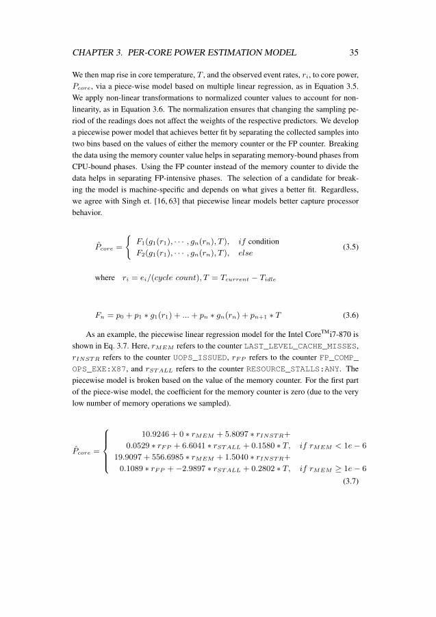
CHAPTER 3. PER-CORE POWER ESTIMATION MODEL 35
We then map rise in core temperature, T , and the observed event rates, ri, to core power,Pcore, via a piece-wise model based on multiple linear regression, as in Equation 3.5.We apply non-linear transformations to normalized counter values to account for non-linearity, as in Equation 3.6. The normalization ensures that changing the sampling pe-riod of the readings does not affect the weights of the respective predictors. We developa piecewise power model that achieves better fit by separating the collected samples intotwo bins based on the values of either the memory counter or the FP counter. Breakingthe data using the memory counter value helps in separating memory-bound phases fromCPU-bound phases. Using the FP counter instead of the memory counter to divide thedata helps in separating FP-intensive phases. The selection of a candidate for break-ing the model is machine-specific and depends on what gives a better fit. Regardless,we agree with Singh et. [16, 63] that piecewise linear models better capture processorbehavior.
P̂core =
{F1(g1(r1), · · · , gn(rn), T ), if conditionF2(g1(r1), · · · , gn(rn), T ), else
(3.5)
where ri = ei/(cycle count), T = Tcurrent − Tidle
Fn = p0 + p1 ∗ g1(r1) + ...+ pn ∗ gn(rn) + pn+1 ∗ T (3.6)
As an example, the piecewise linear regression model for the Intel CoreTMi7-870 isshown in Eq. 3.7. Here, rMEM refers to the counter LAST_LEVEL_CACHE_MISSES,rINSTR refers to the counter UOPS_ISSUED, rFP refers to the counter FP_COMP_OPS_EXE:X87, and rSTALL refers to the counter RESOURCE_STALLS:ANY. Thepiecewise model is broken based on the value of the memory counter. For the first partof the piece-wise model, the coefficient for the memory counter is zero (due to the verylow number of memory operations we sampled).
P̂core =
10.9246 + 0 ∗ rMEM + 5.8097 ∗ rINSTR+
0.0529 ∗ rFP + 6.6041 ∗ rSTALL + 0.1580 ∗ T, if rMEM < 1e− 6
19.9097 + 556.6985 ∗ rMEM + 1.5040 ∗ rINSTR+0.1089 ∗ rFP +−2.9897 ∗ rSTALL + 0.2802 ∗ T, if rMEM ≥ 1e− 6
(3.7)

CHAPTER 3. PER-CORE POWER ESTIMATION MODEL 36
3.4 ValidationWe evaluate our models by estimating per-core power for the SPEC 2006 [71], SPEC-OMP [72, 73], and NAS [74] benchmark suites. In our experiments, we run multi-threaded benchmarks with one thread per core, and single-threaded benchmarks withan instance on each core. We use gcc 4.2 to compile our benchmarks for a 64-bit ar-chitecture with optimization flags enabled, and we run all benchmarks to completion.We use the pfmon utility from the perfmon2 library [75] to access the hardware perfor-mance counters. Table 3.3 gives system details of the machines on which we validatedour power model. System power is based on measuring the power supply’s current drawfrom the power outlet when the machine is idle. When we cannot find published val-ues for idle processor power, we sum power draw when powered off and power savedby turning off cdrom and hard disk drives, removing all but one memory DIMM, anddisconnecting fans. We subtract idle core power from idle system power to get uncore(baseline without processor) power. Change in the uncore power itself (due to DRAMor hard drive accesses, for instance) is included in the model estimations. Including tem-perature as a model input accounts for variation in uncore static power. We always runin the active power state (C0).
We use the sensors utility from the lm-sensors library to obtain core temperatures,and we use the Watts Up? Pro power meter [49] described in Chapter 2 to gather powerdata. This meter is accurate to within 0.1W, and it updates once per second. Althoughmeasuring the power at wall outlet has limitations in terms of sensitivity to fine-grainedchanges in power consumption, we use it for our experiments because of its low cost,non-intrusive use, and easy portability. Moreover, we observe that for the benchmarks inour experiments, the power consumption of the system does not change at the granularityof less than one second, and hence sampling power consumption at the rate of 1 sam-ple/second meets our requirement for this modeling approach. Our modeling approachcan easily be adapted to other power measurement techniques, such as those describedin Chapter 2.
We incorporate the power model into a proof-of-concept, power-aware resourcemanager (a user-level meta-scheduler of Singh et al. [16, 63]) designed to maintain aspecified power envelope. The meta-scheduler manages processes non-invasively, re-quiring no modifications to the applications or OS. It does so by suspending/resumingprocesses and, where supported, applying dynamic voltage/frequency scaling (DVFS)to alter core clock rates. For these experiments, we degrade the system power envelopeby 10%, 20%, and 30% for CoreTMi7-870 platform. Lower envelopes render cores in-active, and thus we do not consider them. Finally, we incorporate the model in a kernelscheduler, implementing a pseudo power sensor per core. The device does not exist

CHAPTER 3. PER-CORE POWER ESTIMATION MODEL 37
(a) Configuration Parameters for Intel Platforms
Intel Q6600 Intel Xeon E5430 Intel CoreTMi7-870Cores/Chips 4, dual dual-core 4Frequency (GHz) 2.4 2.0, 2.66 2.93Process (nm) 65 45 45L1 Instruction 32 KB 8-way 32 KB 8-way 32 KB 4-wayL1 Data 32 KB 8-way 32 KB 8-way 32 KB 8-wayL2 Cache 4 MB 16-way shared 6 MB 16-way shared 256 KB 8-way exclusiveL3 Cache N/A N/A 8 MB 16-way sharedMemory Controller off-chip, 2 channel off-chip, 4 channel on-chip, 2 channelMain Memory 4 GB DDR2-800 8 GB DDR2-800 16 GB DDR3-1333Bus (MHz) 1066 1333 1333Max TDP (W) 105 80 95Linux Kernel 2.6.27 2.6.27 2.6.31Idle System Power (W) 141.0 180.0 54.0Idle Processor Power (W) 38.0 27.0 10.0Idle Temperature (◦C) 36 45 30
(b) Configuration Parameters for AMD Platforms
AMD PhenomTM9500 AMD OpteronTM8212Cores/Chips 4 8, quad dual-coreFrequency (GHz) 1.1, 2.2 2.0Process (nm) 65 90L1 Instruction 64 KB 2-way 64 KB 2-wayL1 Data 64 KB 2-way 64 KB 2-wayL2 Cache 512 KB 8-way exclusive 1024 KB 16-way exclusiveL3 Cache 2 MB 32-way shared N/AMemory Controller on-chip, 2 channel on-chip, 2 channelMain Memory 4 GB DDR2-800 16 GB DDR2-667Bus (MHz) 1100, 2200 1000Max TDP (W) 95 95Linux Kernel 2.6.25 2.6.31Idle System Power (W) 84.1 302.6Idle Processor Power (W) 20.1 53.6WIdle Temperature (◦C) 36 33
Table 3.3: Machine Configuration Parameters
(a) PMCs Selected for Intel Platforms
Category Intel Q6600 Intel E5430 Intel CoreTMi7-870
Memory L2_LINES_IN LAST_LEVEL_CACHE_MISSES LAST_LEVEL_CACHE_MISSESInstructions Executed UOPS_RETIRED UOPS_RETIRED UOPS_ISSUEDFloating Point X87_OPS_RETIRED X87_OPS_RETIRED FP_COMP_OPS_EXE:X87Stalls RESOURCE_STALLS RESOURCE_STALLS RESOURCE_STALLS:ANY
(b) PMCs Selected for AMD Platforms
Category AMD PhenomTM9500 AMD OpteronTM8212
Memory L2_CACHE_MISS DATA_CACHE_ACCESSESInstructions Executed RETIRED_UOPS RETIRED_INSTRUCTIONSFloating Point RETIRED_MMX_AND_FP_INSTRUCTIONS DISPATCHED_FPU:OPS_MULTIPLYStalls DISPATCH_STALLS DECODER_EMPTY
Table 3.4: PMCs Selected for Power-Estimation Model
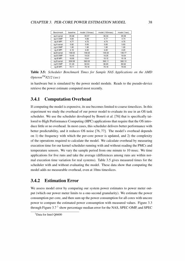
CHAPTER 3. PER-CORE POWER ESTIMATION MODEL 38
Benchmark baseline model (10msec) model (100msec) model (1sec)
ep.A serial 35.68 35.57 36.04 35.59ep.A OMP 4.84 4.89 4.77 4.74ep.A MPI 4.77 4.72 4.73 4.75
cg.A serial 5.82 5.83 5.83 5.83cg.A OMP 1.95 1.95 1.95 1.95cg.A MPI 2.19 2.20 2.20 2.20
ep.B serial 146.53 146.52 145.52 146.77ep.B OMP 19.45 19.33 19.35 19.54ep.B MPI 18.95 19.41 19.12 19.18
cg.B serial 559.58 560.50 560.11 560.10cg.B OMP 91.29 92.64 96.90 89.92cg.B MPI 79.11 79.18 79.18 79.05
Table 3.5: Scheduler Benchmark Times for Sample NAS Applications on the AMD
OpteronTM8212 (sec)
in hardware but is simulated by the power model module. Reads to the pseudo-deviceretrieve the power estimate computed most recently.
3.4.1 Computation OverheadIf computing the model is expensive, its use becomes limited to coarse timeslices. In thisexperiment we study the overhead of our power model to evaluate its use in an OS taskscheduler. We use the scheduler developed by Boneti et al. [76] that is specifically tai-lored to High Performance Computing (HPC) applications that require that the OS intro-duce little or no overhead. In most cases, this scheduler delivers better performance withbetter predictability, and it reduces OS noise [76, 77]. The model’s overhead dependson 1) the frequency with which the per-core power is updated, and 2) the complexityof the operations required to calculate the model. We calculate overhead by measuringexecution time for our kernel scheduler running with and without reading the PMCs andtemperature sensors. We vary the sample period from one minute to 10 msec. We timeapplications for five runs and take the average (differences among runs are within nor-mal execution time variation for real systems). Table 3.5 gives measured times for thescheduler with and without evaluating the model. These data show that computing themodel adds no measurable overhead, even at 10ms timeslices.
3.4.2 Estimation ErrorWe assess model error by comparing our system power estimates to power meter out-put (which our power meter limits to a one-second granularity). We estimate the powerconsumption per core, and then sum up the power consumption for all cores with uncorepower to compare the estimated power consumption with measured values. Figure 3.3through Figure 3.7 1 show percentage median error for the NAS, SPEC-OMP, and SPEC
1Data for Intel Q6600
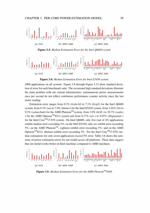
CHAPTER 3. PER-CORE POWER ESTIMATION MODEL 39
bt cg ep ft lulu-h
pm
g sp ua0
2
4
6
8
10
% M
edia
n E
rro
r
(a) NAS
amm
p
applu
apsi ar
t
fma3
d
mgr
id
quak
e
swim
wup
wise
0
2
4
6
8
10
% M
ed
ian
Err
or
(b) SPEC-OMP
asta
r
bwav
es
bzip2
cactus
ADM
calculix
dealll
gam
ess
gcc
Gem
sFDTD
gobm
k
grom
acs
h264
ref
hmm
erlbm
leslie3d
libqu
antu
mm
cfm
ilc
nam
d
omne
tpp
perlb
ench
povr
ay
sjen
g
soplex
xalanc
bmk
zeus
mp
0
2
4
6
8
10
% M
edia
n E
rror
(c) SPEC 2006
Figure 3.3: Median Estimation Error for the Intel Q6600 system
bt cg ep ft lulu-h
pm
g sp ua0
2
4
6
8
10
% M
ed
ian
Err
or
(a) NAS
amm
p
applu
apsi ar
t
fma3
d
mgr
id
quak
e
swim
wup
wise
0
2
4
6
8
10
% M
ed
ian
Err
or
(b) SPEC-OMP
asta
r
bwav
es
bzip2
cactus
ADM
calculix
dealll
gam
ess
gcc
Gem
sFDTD
gobm
k
grom
acs
h264
ref
hmm
erlbm
leslie3d
libqu
antu
mm
cfm
ilc
nam
d
omne
tpp
perlb
ench
povr
ay
sjen
g
soplex
xalanc
bmk
zeus
mp
0
2
4
6
8
10
% M
edia
n E
rror
(c) SPEC 2006
Figure 3.4: Median Estimation Error for Intel E5430 system
2006 applications on all systems. Figure 3.8 through Figure 3.12 show standard devia-tion of error for each benchmark suite. The occasional high standard deviations illustratethe main problem with our current infrastructure: instantaneous power measurementsonce per second do not reflect continuous performance counter activity since the lastmeter reading.
Estimation error ranges from 0.3% (leslie3d) to 7.1% (bzip2) for the Intel Q6600system, from 0.3% (ua) to 7.0% (hmmer) for the Intel E5430 system, from 1.02% (bt) to9.3% (xalancbmk) for the AMD PhenomTMsystem, from 1.0% (bt.B ) to 10.7% (soplex) for the AMD OpteronTM8212 system and from 0.17% (art ) to 9.07% (libquantum )for the Intel CoreTMi7-870 system. On Intel Q6600, only five (out of 45) applicationsexhibit median error exceeding 5%; on the Intel E5430, only six exhibit error exceeding5%; on the AMD PhenomTM, eighteen exhibit error exceeding 5%; and on the AMDOpteronTM8212, thirteen exhibit error exceeding 5%. For the Intel CoreTMi7-870, me-dian estimations for only seven applications exceed 5% error. Table 3.6 shows the sum-mary of power estimation errors for our model across all platforms. These data suggessthat our model works better on Intel machines compared to AMD machines.
bt cg ep ft lulu-h
pm
g sp ua0
2
4
6
8
10
% M
ed
ian
Err
or
(a) NAS
amm
p
applu
apsi ar
t
fma3
d
gafo
rt
mgr
id
quak
e
swim
wup
wise
0
2
4
6
8
10
% M
ed
ian
Err
or
(b) SPEC-OMP
asta
r
bwav
es
bzip2
cactus
ADM
calculix
dealll
gam
ess
gcc
Gem
sFDTD
gobm
k
grom
acs
h264
ref
hmm
erlbm
leslie3d
libqu
antu
mm
cfm
ilc
nam
d
omne
tpp
perlb
ench
povr
ay
sjen
g
soplex
xalanc
bmk
zeus
mp
0
2
4
6
8
10
% M
edia
n E
rror
(c) SPEC 2006
Figure 3.5: Median Estimation Error for the AMD PhenomTM9500

CHAPTER 3. PER-CORE POWER ESTIMATION MODEL 40
bt cg ep ft lulu-h
pm
g sp ua0
2
4
6
8
10
% M
edia
n E
rro
r
(a) NAS
amm
p
applu
apsi ar
t
fma3
d
gafo
rt
mgr
id
quak
e
swim
wup
wise
0
2
4
6
8
10
% M
ed
ian E
rror
(b) SPEC-OMP
asta
r
bwav
es
bzip2
cactus
ADM
calculix
dealll
gam
ess
gcc
Gem
sFDTD
gobm
k
grom
acs
h264
ref
hmm
erlbm
leslie3d
libqu
antu
mm
cfm
ilc
nam
d
omne
tpp
perlb
ench
povr
ay
sjen
g
soplex
xalanc
bmk
zeus
mp
0
2
4
6
8
10
% M
edia
n E
rror
(c) SPEC 2006
Figure 3.6: Median Estimation Error for the AMD OpteronTM8212
bt cg ep ft lulu-h
pm
g sp ua0
2
4
6
8
10
% M
ed
ian
Err
or
(a) NAS
amm
p
applu
apsi ar
t
fma3
d
mgr
id
quak
e
swim
wup
wise
0
2
4
6
8
10
% M
ed
ian
Err
or
(b) SPEC-OMP
asta
r
bwav
es
bzip2
cactus
ADM
calculix
dealll
gam
ess
gcc
Gem
sFDTD
gobm
k
grom
acs
h264
ref
hmm
erlbm
leslie3d
libqu
antu
mm
cfm
ilc
nam
d
omne
tpp
perlb
ench
povr
ay
sjen
g
soplex
xalanc
bmk
zeus
mp
0
2
4
6
8
10
% M
edia
n E
rror
(c) SPEC 2006
Figure 3.7: Median Estimation Error for the Intel CoreTMi7
bt cg ep ft lulu-h
pm
g sp ua0
2
4
6
8
10
% S
D
(a) NAS
amm
p
applu
apsi ar
t
fma3
d
gafo
rt
mgr
id
quak
e
swim
wup
wise
0
2
4
6
8
10
% S
D
(b) SPEC-OMP
asta
r
bwav
es
bzip2
cactus
ADM
calculix
dealll
gam
ess
gcc
Gem
sFDTD
gobm
k
grom
acs
h264
ref
hmm
erlbm
leslie3d
libqu
antu
mm
cfm
ilc
nam
d
omne
tpp
perlb
ench
povr
ay
sjen
g
soplex
xalanc
bmk
zeus
mp
0
2
4
6
8
10
% S
D
(c) SPEC 2006
Figure 3.8: Standard Deviation of Error for the Intel Q6600 system
bt cg ep ft lulu-h
pm
g sp ua0
2
4
6
8
10
% S
D
(a) NAS
amm
p
applu
apsi ar
t
fma3
d
gafo
rt
mgr
id
quak
e
swim
wup
wise
0
2
4
6
8
10
% S
D
(b) SPEC-OMP
asta
r
bwav
es
bzip2
cactus
ADM
calculix
dealll
gam
ess
gcc
Gem
sFDTD
gobm
k
grom
acs
h264
ref
hmm
erlbm
leslie3d
libqu
antu
mm
cfm
ilc
nam
d
omne
tpp
perlb
ench
povr
ay
sjen
g
soplex
xalanc
bmk
zeus
mp
0
2
4
6
8
10
% S
D
(c) SPEC 2006
Figure 3.9: Standard Deviation of Error for Intel E5430 system
Benchmark Intel Q660 Intel E5430 Intel CoreTMi7-870 AMD PhenomTM AMD 8212
SPEC 2006 1.1 2.8 2.22 3.5 4.80NAS 1.6 3.9 3.11 4.5 2.55SPEC OMP 1.6 3.5 2.02 5.2 3.35Overall 1.2 3.6 2.07 3.8 4.38
Table 3.6: Estimation Error Summary

CHAPTER 3. PER-CORE POWER ESTIMATION MODEL 41
bt cg ep ft lulu-h
pm
g sp ua0
2
4
6
8
10
% S
D
11.7
19.3
15.6
(a) NAS
amm
p
applu
apsi ar
t
fma3
d
gafo
rt
mgr
id
quak
e
swim
wup
wise
0
2
4
6
8
10
% S
D(b) SPEC-OMP
asta
r
bwav
es
bzip2
cactus
ADM
calculix
dealll
gam
ess
gcc
Gem
sFDTD
gobm
k
grom
acs
h264
ref
hmm
erlbm
leslie3d
libqu
antu
mm
cfm
ilc
nam
d
omne
tpp
perlb
ench
povr
ay
sjen
g
soplex
xalanc
bmk
zeus
mp
0
2
4
6
8
10
% S
D
14.9
12.2
(c) SPEC 2006
Figure 3.10: Standard Deviation of Error for the AMD PhenomTM9500
bt cg ep ft lulu-h
pm
g sp ua0
2
4
6
8
10
% S
D
(a) NAS
amm
p
applu
apsi ar
t
fma3
d
gafo
rt
mgr
id
quak
e
swim
wup
wise
0
2
4
6
8
10
% S
D
(b) SPEC-OMP
asta
r
bwav
es
bzip2
cactus
ADM
calculix
dealll
gam
ess
gcc
Gem
sFDTD
gobm
k
grom
acs
h264
ref
hmm
erlbm
leslie3d
libqu
antu
mm
cfm
ilc
nam
d
omne
tpp
perlb
ench
povr
ay
sjen
g
soplex
xalanc
bmk
zeus
mp
0
2
4
6
8
10
% S
D
(c) SPEC 2006
Figure 3.11: Standard Deviation of Error for the AMD OpteronTM8212
bt cg ep ft lulu-h
pm
g sp ua0
2
4
6
8
10
% S
D
(a) NAS
amm
p
applu
apsi ar
t
fma3
d
gafo
rt
mgr
id
quak
e
swim
wup
wise
0
2
4
6
8
10
% S
D
(b) SPEC-OMP
asta
r
bwav
es
bzip2
cactus
ADM
calculix
dealll
gam
ess
gcc
Gem
sFDTD
gobm
k
grom
acs
h264
ref
hmm
erlbm
leslie3d
libqu
antu
mm
cfm
ilc
nam
d
omne
tpp
perlb
ench
povr
ay
sjen
g
soplex
xalanc
bmk
zeus
mp
0
2
4
6
8
10
% S
D
(c) SPEC 2006
Figure 3.12: Standard Deviation of Error for the IntelCoreTMi7

CHAPTER 3. PER-CORE POWER ESTIMATION MODEL 42
0 10 20 30
% Error
0.0
0.2
0.4
0.6
0.8
1.0
Fra
ctio
n o
f S
pa
ce
Co
ve
red
(a) Intel Q6600
0 10 20 30
% Error
0.0
0.2
0.4
0.6
0.8
1.0
Fra
ctio
n o
f S
pa
ce
Co
ve
red
(b) Intel E5430
0 10 20 30
% Error
0.0
0.2
0.4
0.6
0.8
1.0
Fra
ctio
n o
f S
pa
ce
Co
ve
red
(c) AMD 9500
0 10 20 30
% Error
0.0
0.2
0.4
0.6
0.8
1.0
Fra
ctio
n o
f S
pa
ce
Co
ve
red
(d) AMD 8212
0 10 20 30
% Error
0.0
0.2
0.4
0.6
0.8
1.0
Fra
ctio
n o
f S
pa
ce
Co
ve
red
(e) CoreTMi7
Figure 3.13: Cumulative Distribution Function (CDF) Plots Showing Fraction of Space
Predicted (y axis) under a Given Error (x axis) for Each System
bt cg ep ft lulu-h
pm
g sp ua15
20
25
30
35
Po
we
r (W
)
actual
predicted
(a) NAS
amm
p
applu
apsi ar
t
fma3
d
mgr
id
quak
e
swim
wup
wise
15
20
25
30
35
Po
we
r (W
)
actual
predicted
(b) SPEC-OMP
asta
r
bwav
es
bzip2
cactus
ADM
calculix
dealll
gam
ess
gcc
Gem
sFDTD
gobm
k
grom
acs
h264
ref
hmm
erlbm
leslie3d
libqu
antu
mm
cfm
ilc
nam
d
omne
tpp
perlb
ench
povr
ay
sjen
g
soplex
xalanc
bmk
zeus
mp
15
20
25
30
35
Pow
er
(W)
actual
predicted
(c) SPEC 2006
Figure 3.14: Estimated versus Measured Error for the Intel Q6600 system
Figure 3.13 shows model coverage via Cumulative Distribution Function (CDF)plots for the suites. On Q6600, 85% of estimates have less than 5% error, and 98%have less than 10%. On E5430, 73% have less than 5% error, and 99% less than 10%.On PhenomTM, 59% have less than 5% error, and 92% less than 10%. On 8212, 37%have less than 5% error, and 76% have less than 10%. For the CoreTMi7-870, 82% ofestimates have less than 5% error and 96% have less than 10% error. The vast majorityof estimates exhibit very small error.
These errors are not excessive, but lower is better. Prediction errors are not clus-tered, but are spread throughout application execution. Model accuracy depends on the
bt cg ep ft lulu-h
pm
g sp ua15
20
25
30
35
Po
we
r (W
)
actual
predicted
(a) NAS
amm
p
applu
apsi ar
t
fma3
d
gafo
rt
mgr
id
quak
e
swim
wup
wise
15
20
25
30
35
Po
we
r (W
)
actual
predicted
(b) SPEC-OMP
asta
r
bwav
es
bzip2
cactus
ADM
calculix
dealll
gam
ess
gcc
Gem
sFDTD
gobm
k
grom
acs
h264
ref
hmm
erlbm
leslie3d
libqu
antu
mm
cfm
ilc
nam
d
omne
tpp
perlb
ench
povr
ay
sjen
g
soplex
xalanc
bmk
zeus
mp
15
20
25
30
35
Pow
er
(W)
actual
predicted
(c) SPEC 2006
Figure 3.15: Estimated versus Measured Error for Intel E5430 system

CHAPTER 3. PER-CORE POWER ESTIMATION MODEL 43
bt cg ep ft lulu-h
pm
g sp ua15
20
25
30
35
Pow
er
(W)
actual
predicted
(a) NAS
amm
p
applu
apsi ar
t
fma3
d
gafo
rt
mgr
id
quak
e
swim
wup
wise
15
20
25
30
35
Po
wer
(W)
actual
predicted
(b) SPEC-OMP
asta
r
bwav
es
bzip2
cactus
ADM
calculix
dealll
gam
ess
gcc
Gem
sFDTD
gobm
k
grom
acs
h264
ref
hmm
erlbm
leslie3d
libqu
antu
mm
cfm
ilc
nam
d
omne
tpp
perlb
ench
povr
ay
sjen
g
soplex
xalanc
bmk
zeus
mp
15
20
25
30
35
Pow
er
(W)
actual
predicted
(c) SPEC 2006
Figure 3.16: Estimated versus Measured Error for the AMD PhenomTM9500
bt cg ep ft lulu-h
pm
g sp ua30
35
40
45
50
Po
we
r (W
)
actual
predicted
(a) NAS
amm
p
applu
apsi ar
t
fma3
d
gafo
rt
mgr
id
quak
e
swim
wup
wise
30
35
40
45
50
Po
we
r (W
)
actual
predicted
(b) SPEC-OMP
asta
r
bwav
es
bzip2
cactus
ADM
calculix
dealll
gam
ess
gcc
Gem
sFDTD
gobm
k
grom
acs
h264
ref
hmm
erlbm
leslie3d
libqu
antu
mm
cfm
ilc
nam
d
omne
tpp
perlb
ench
povr
ay
sjen
g
soplex
xalanc
bmk
zeus
mp
30
35
40
45
50
Pow
er
(W)
actual
predicted
(c) SPEC 2006
Figure 3.17: Estimated versus Measured Error for the AMD OpteronTM8212
bt cg ep ft lulu-h
pm
g sp ua15
20
25
30
35
Po
we
r (W
)
actual
predicted
(a) NAS
amm
p
applu
apsi ar
t
fma3
d
mgr
id
quak
e
swim
wup
wise
15
20
25
30
35
Po
we
r (W
)
actual
predicted
(b) SPEC-OMP
asta
r
bwav
es
bzip2
cactus
ADM
calculix
dealll
gam
ess
gcc
Gem
sFDTD
gobm
k
grom
acs
h264
ref
hmm
erlbm
leslie3d
libqu
antu
mm
cfm
ilc
nam
d
omne
tpp
perlb
ench
povr
ay
sjen
g
soplex
xalanc
bmk
zeus
mp
15
20
25
30
35
Pow
er
(W)
actual
predicted
(c) SPEC 2006
Figure 3.18: Estimated versus Measured Error for the Intel CoreTMi7-870

CHAPTER 3. PER-CORE POWER ESTIMATION MODEL 44
particular PMCs available on a given platform. If available PMCs do not sufficientlyrepresent the microarchitecture, model accuracy will suffer. For example, the AMDOpteronTM8212 processor supports no single counter giving total floating point oper-ations. Instead, separate PMCs track different types of floating point operations. Wetherefore choose the one most highly correlated with power. Model accuracy wouldlikely improve if a single PMC reflecting all floating point operations were available. Forprocessor models supporting only two Model Specific Registers for reading PMC val-ues, capturing the activity of four counters requires multiplexing the counting of PMC-related events. This means that events are counted for only half a second (or half thetotal sampling period), and are doubled to estimate the value over the entire period. Thisapproximation can introduce inaccuracies when program behavior is changing rapidly.The model estimation accuracy is also affected by accuracy of hardware sensors. Forinstance, the OpteronTM8212 temperature sensor data suffers with low accuracy [78].
Similarly, even though the microbenchmark tries to cover all scenarios of powerconsumption, the resulting regression model will represent a generalized case. This isespecially true for a model that tries to estimate power for a complex microarchitectureusing limited number of counters. For example, floating point operations can consist ofadd, multiply, or divide operations, all of which use different execution units and henceconsume a different amounts of power. If the application being studied uses operationsnot covered by the training microbenchmark, model accuracy could also suffer.
A model can be no more accurate than the information used to build it. Performancecounter implementations display nondeterminism [66] and error [64]. All of these im-pact model accuracy. Given all these sources of inaccuracy, there seems little need formore complex, sophisticated mathematics when building a model.
3.5 ManagementIn the previous section, we discussed our approach to estimating the power consumptionof processor resources using power modeling. In this section, we discuss the use of ourpower model by resource managers that perform task scheduling.
To demonstrate one use of our on-line power model, we experiment with the user-level meta-scheduler from Singh et al. [16, 63]. This live power management applica-tion maintains a user-defined system power budget by power-aware scheduling of tasksand/or by using DVFS. We use the power model to compute core power consumptiondynamically. The application spawns one process per core. The scheduler reads PMCvalues via pfmon and feeds the sampled PMC values to the power model to estimate corepower consumption.
The meta-scheduler binds the affinity of the processes to a particular core to simplify

CHAPTER 3. PER-CORE POWER ESTIMATION MODEL 45
Start
Assign one task
per processor
Check for power
envelope breach
Envelope
breached?
Suspend a running
process as per
scheduling policy
Apply DVFS to
lower frequency
one step
Lowest
Frequency?
Apply DVFS to
increase frequency
one step
Resume a suspended
process as per
scheduling policy
X ms Delay
Highest
Frequency?
Any process
suspended?
YesNo Yes
NoNo
NoYes
Yes
Figure 3.19: Flow diagram for the Meta-Scheduler
task management and power estimation. It dynamically calculates power values at a setinterval (one second, in our case) and compares the system-power envelope with the sumof power for all cores together with the uncore power.
When the scheduler detects a breach in the power envelope, it takes steps to controlthe power consumption. The scheduler employs two knobs to control system-powerconsumption: dynamic voltage-frequency scaling as a fine knob, and process suspensionas a coarse knob. When the envelope is breached, the scheduler first tries to lower thepower consumption by scaling down the frequency. If power consumption remains toohigh, the scheduler starts suspending processes to meet the envelope’s demands. Thescheduler maintains the record of the power being consumed by the process at the timeof suspension. When the estimated power consumption is less than the target powerenvelope, the scheduler checks whether any of the suspended processes can be resumedbased on the power they were consuming at the time of suspension. If the gap betweenthe current power consumption and the target power budget is not enough to resume asuspended process, and if the processor is operating at a frequency lower than maximum,the scheduler scales up the voltage-frequency. Fig. 3.19 shows the flow diagram of themeta-scheduler.
3.5.1 Sample PoliciesWhen the scheduler suspends a process, it tries to choose the process that will have theleast impact on completion time of all the processes. We explore the use of our powermodel in a scheduler via two sample policies for process suspension.
The Throughput policy targets maximum power efficiency (max instructions/watt)under a given power envelope. When the envelope is breached, the scheduler calculates

CHAPTER 3. PER-CORE POWER ESTIMATION MODEL 46
Benchmark Category Benchmark Applications Peak System Power (W)
CPU-Bound ep, gamess, namd, povray 130
Moderate art, lu, wupwise, xalancbmk 135
Memory-Bound astar, mcf, milc, soplex 130
Table 3.7: Workloads for Scheduler Evaluation
the ratio of instructions/UOPS retired to the power consumed for each core and suspendsthe process having committed the fewest instructions per watt of power consumed. Whenresuming a process, it selects the process (if there is more than one suspended process)that had committed the maximum instructions/watt at the time of suspension. This policyfavors processes that are less often stalled while waiting for load operations to complete.This policy thus favors CPU bound applications.
The Fairness policy divides the available power budget equally among all processes.When applying this policy, the scheduler maintains a running average of the powerconsumed by each core. When the scheduler must choose a process for suspension,it chooses the process having consumed the most average power. For resumption, thescheduler chooses the process that had consumed the least average power at the timeof suspension. This policy strives to regulate core temperature, since it throttles coresconsuming the most average power. Since there is high correlation between core powerconsumption and core temperature, this makes sure that the core with highest tempera-ture receives time to cool down, while cores with lower temperature continue working.Since memory-bound applications are stalled more often, they consume less averagepower, and so this policy favors memory-bound applications.
3.5.2 Experimental SetupFor the scheduler experiments, we use an Intel CoreTMi7-870 system, using DVFS tovary frequencies between 2.926, 2.66, 2.394, 2.128, 1.862, 1.596 and 1.33 GHz. Weform separate power models for different frequencies. The power manager can thusbetter implement policy decisions by estimating power for each frequency. If all corefrequencies have been reduced but the power envelope is still breached, we suspendprocesses to reduce power. We compare against runtimes with no enforced power enve-lope. We divide our workloads into three sets based on CPU intensity. We define CPUintensity as the ratio of instructions retired to last-level cache misses. The three setsare designated as CPU-Bound, Moderate, and Memory-Bound workloads (in decreasingorder of CPU intensity). The workloads categorized in these sets are listed in Table 3.7.

CHAPTER 3. PER-CORE POWER ESTIMATION MODEL 47
70% 80% 90% 100%
% Power Budget
0
1
2
Norm
aliz
ed R
un T
ime
Throughput
Fairness
(a) CPU-bound
70% 80% 90% 100%
% Power Budget
0
1
2
Norm
aliz
ed R
un T
ime
Throughput
Fairness
(b) Memory-bound
70% 80% 90% 100%
% Power Budget
0
1
2N
orm
aliz
ed R
un T
ime
Throughput
Fairness
(c) Moderate
Figure 3.20: Runtimes for Workloads on the Intel CoreTMi7-870 (without DVFS)
3.5.3 ResultsFig. 3.20 shows the normalized runtimes for all the workloads when only process sus-pension is used to maintain the power envelope. The Throughput policy should favorCPU-bound workloads, while the Fairness policy should favor memory bound work-loads, but this distinction is not always visible. This is because of the differences in theruntimes of the various workloads. This can be seen from the execution times of theCPU-bound benchmarks when using the Throughput policy. The CPU bound applica-tions ep and gamess have the lowest computational intensities and execution times. Asa result, these two applications are suspended most frequently, which does not affect thetotal execution time, even when the power envelope is set to 80% of peak usage.
Fig. 3.21 shows the results when the scheduler uses both DVFS and process sus-pension to maintain the given power envelope. As noted, the scheduler uses DVFS asa fine knob and process suspension as a coarse knob in maintaining the envelope. TheIntel CoreTMi7-870 processor that we use for our experiments supports fourteen differentvoltage-frequency points. These frequency points range from 2.926 GHz to 1.197 GHz.For our experiments, we make models for seven frequency points (2.926, 2.66, 2.394,2.128, 1.862, 1.596 and 1.33 GHz), and we adjust the processor frequency across thesepoints. Our experimental results show that for CPU-bound and moderate benchmarks,there is little difference in execution time under different suspension policies. This sug-gests that for these applications, the scheduler hardly needs to suspend the processes andregulating DVFS points proves sufficient to maintain the power envelope. Performancefor DVFS degrades compared to cases where no DVFS is used. The explanation for

CHAPTER 3. PER-CORE POWER ESTIMATION MODEL 48
70% 80% 90% 100%
% Power Budget
0
1
2
Norm
aliz
ed R
un T
ime
Throughput
Fairness
(a) CPU-bound
70% 80% 90% 100%
% Power Budget
0
1
2
Norm
aliz
ed R
un T
ime
Throughput
Fairness
(b) Memory-bound
70% 80% 90% 100%
% Power Budget
0
1
2N
orm
aliz
ed R
un T
ime
Throughput
Fairness
(c) Moderate
Figure 3.21: Runtimes for Workloads on the Intel CoreTMi7-870 (with DVFS)
this lies in the difference between runtimes of different applications within the workloadsets. When no DVFS is used, all processes run at full speed. And even when one of theprocesses is suspended, if that process is not critical, it still runs at full speed later inparallel with the critical process. But in the case of DVFS being given higher priorityover process suspension, when the envelope is breached, all processes are slowed, andthis affects total execution time.
3.5.4 Related WorkMuch previous work leverages performance counters for power estimation. Our work isbased on the approach of Singh et al. [16,63]; we augment that work by porting and val-idating the model on many platforms, improving accuracy of the model by augmentingthe microbenchmark and counter selection methodology, analyzing estimation errors,and exploiting multiple DVFS operating points for scheduler validation.
Joseph and Martonosi [10] use PMCs to estimate power in a simulator (SimpleScalar [79])and on real hardware (a Pentium Pro). Their hardware supports two PMCs, while theyrequire twelve. They perform multiple benchmark runs to collect data, forming themodel offline. Multiplexing twelve PMCs would require program behavior to be rela-tively constant across the entire sampling interval. They cannot estimate power for 24%of the chip, and so they assume peak power for those structures.
Contreras and Martonosi [14] use five PMCs to estimate power for different frequen-cies on an XScale system (with an in-order uniprocessor). Like Joseph and Martonosi,they gather data from multiple benchmark runs. They derive power weights for frequency-

CHAPTER 3. PER-CORE POWER ESTIMATION MODEL 49
voltage pairs, and form a parameterized linear model. Their model exhibits low percent-age error, like ours, but they test on only seven applications, and their methodologyis only demonstrated for a single platform. This methodology, like that of Joseph andMartonosi, is not intended for on-line use.
Economou et al. [15] use PMCs to predict power on a blade server. They profile thesystem using application-independent microbenchmarks. The resulting model estimatespower for the CPU, memory, and hard drive with 10% average error. Wu et al. [80] alsouse microbenchmarks to develop a model using a variable number of PMCs to estimateactive power of Pentium 4 functional units. They measure CPU power with a clamp-onammeter. Such invasive approaches are neither applicable to systems in the field, norscalable to HPC clusters.
Merkel and Bellosa [81] use PMCs to estimate power per processor in an eight-waySMP, shuffling processes to reduce overheating of individual processors. They do notstate which PMCs they use, nor how they are chosen. Their goal is not to reduce power,but to distribute it. Their estimation method suffers less than 10% error in a linux kernelimplementation.
Lee and Brooks [18] predict power via statistical inference models. They buildcorrelations based on hardware parameters, using the most significant parameters to traintheir model. They profile their design space a priori, and then estimate power on randomsamples. This methodology requires training on the same applications for which theywant to estimate power, and so their approach depends on having already sampled allapplications of interest.
Spiliopoulos et al. [23] use instructions executed and instructions retired counter todevelop a power model. Their model shows high errors for memory-bound benchmarkssince they do not consider memory operations in their model.
Instead of applying DVFS per core, Rangan et al. [19] study thread placement andmigration among independent voltage and frequency domains. This thread motion per-mits much finer-grain control over power management and delivers better performancethan conventional DVFS for a given power budget. Grochowski et al. [82] study fourmethods to control energy per instruction (EPI), finding that a combination of VFS andasymmetric cores offers the most promising approach to balancing latency and through-put in an energy-constrained environment. Annavaram et al. [83] leverage this work tothrottle EPI by scheduling multithreaded tasks on an asymmetric CMP, using more EPIin periods of low parallelism to make better use of a fixed power budget.
Rajamani et al. [11] use their power estimation model to drive a power managementpolicy called PerformanceMaximizer. For a given power budget, they exploit the DVFSlevels of the processor to try to maximize the processor performance. For each per-formance state (P-state), they apply their power model to estimate power consumption
CHAPTER 3. PER-CORE POWER ESTIMATION MODEL 50
at the current P-state. They use the calculated power value to estimate the power con-sumption at other P-states by linearly scaling the current power value with frequency.The scheduler increases the performance state to highest level that it estimates would besafely below the power budget value.
Banikazemi et al. [20] use a power-aware meta-scheduler. Their meta-schedulermonitors the performance, power and energy of the system by using performance coun-ters and in-built power monitoring hardware. It uses this information to dynamicallyremap the software threads on multi-core servers for higher performance and lower en-ergy usage. Their framework is flexible enough to substitute the hardware power monitorwith a performance-counter based model.
Isci et al. [21] analyze global power management policies to enforce a given powerbudget and to minimize power consumption for the given performance target. Theyconduct their experiments on the Turandot [84] simulator. They assume the presence ofon-core current sensors to acquire core power information, while they use performancecounters to gather core performance information. They have developed a global powermanager that periodically monitors the power and performance of each core and sets theoperating mode (akin to DVFS performance states) of the core for the next monitoringinterval. They assume that the power mode can be set independently for each core. Theyexperiment with three policies to evaluate their global power manager. The Prioritypolicy assigns different priorities to different cores in a multi-core processor and triesto speed up the core with highest priority while slowing down the lowest priority corewhen the the power consumption overshoots the assigned budget. The policy calledpullHipushLo is similar to our Fairness policy from the above case study; it tries tobalance the power consumption of each core by slowing down the core with highestpower consumption when the power budget is exceeded and speeds up the core withlowest power consumption when there is a power surplus. MaxBIPS tries to maximizethe system throughput by choosing the combination of power modes on different coresthat is predicted to provide maximum overall BIPS (Billion Instructions Per Second).
Meng et al. [22] apply a multi-optimization power saving strategy to meet the con-straints of a chip-wide power budget on reconfigurable processors. They run a globalpower manager that configures the CPU frequency and/or cache size of individual cores.They use risk analysis to evaluate the trade-offs between power saving optimizationsand potential performance loss. They select the power-saving strategies at design timeto create a static pool of candidate optimizations. They make an analytic power andperformance model using performance counters and sensors that allows them to quicklyevaluate many power modes and enables their power manager to choose a global powermode at periodic intervals that can obey the processor-wide power budget while maxi-mizing the throughput.

CHAPTER 3. PER-CORE POWER ESTIMATION MODEL 51
3.6 ConclusionWe derive statistical, piece-wise multiple linear regression power models mapping PMCvalues and temperature readings to power, and demonstrate their accuracy for the SPEC2006, SPEC-OMP, and NAS benchmark suites. We write microbenchmarks to exercisethe PMCs in order to characterize the machine and run those microbenchmarks with apower meter plugged in to generate data for building the models. For our regressionmodels, we select the PMCs that correlate most strongly with measured power. Be-cause they are built on microbenchmark data, and not actual workload data, the resultingmodels are application independent. We apply the models to 45 benchmarks (includingmultithreaded applications) on five CMPs containing dual- or quad-core chips totalingfour or eight cores. In spite of our generality, estimation errors are consistently lowacross five different systems. We observe overall median errors per machine between1.2% and 4.4%.
We then show the effectiveness of our power model for live power management onan Intel CoreTMsystem with and without DVFS. We suspend and resume processes basedon per-core power usage, ensuring that a given power envelope is not breached. We alsoscale core frequencies to remain under the power envelope.
As numbers of cores and power demands continue to grow, efficient computing re-quires better methods for managing individual resources. The per-core power estimationmethodology presented here extends previously published models in both breadth anddepth, and represents a promising tool for helping meet those challenges, both by pro-viding useful information to resource managers and by highlighting opportunities forimproving hardware support for energy-aware resource management. Such support isessential for fine-grained, power-aware resource management.

4Characterization of Intel’s Restricted
Transactional Memory
4.1 IntroductionTransactional memory (TM) [85] simplifies some of the challenges of shared-memoryprogramming. The responsibility for maintaining mutual exclusion over arbitrary sets ofshared-memory locations is devolved to the TM system, which may be implemented insoftware (STM) or hardware (HTM). TM presents the programmer with fairly easy-to-use programming constructs that define a transaction — a piece of code whose executionis guaranteed to appear as if it occurred atomically and in isolation.
The research community has explored this design space in depth, and a variety ofproposed systems take advantage of transaction characteristics to simplify implementa-tion and improve performance [86–89]. Hardware support for transactional memory hasbeen implemented in Rock [90] from Sun Microsystems, Vega from Azul Systems [91],and Blue Gene/Q [92] and System z [93] from IBM. Haswell is the first Intel product toprovide such hardware support. Intel’s Transactional Synchronization Extensions (TSX)allow programmers to run transactions on a best-effort HTM implementation, i.e., the
52

CHAPTER 4. CHARACTERIZATION OF INTEL’S RTM 53
platform provides no guarantees that hardware transactions will commit successfully,and thus the programmer must provide a non-transactional path as a fallback mecha-nism. Intel TSX supports two software interfaces to execute atomic blocks: HardwareLock Elision (HLE) is an instruction set extension to run atomic blocks on legacy hard-ware, and Restricted Transactional Memory (RTM) is a new instruction set interface toexecute transactions on the underlying TSX hardware.
The previous chapters have highlighted the need for better hardware introspectioninto power consumption. As better hardware support for such introspection becomesavailable, it is important to evaluate accuracy and acuity so that users can choose amongvarious combinations of measurement and modeling techniques. Since Intel’s Core i74770 microarchitecture is among the first to support both power modeling and supportfor transactional memory, it makes an interesting platform for analyzing power/perfor-mance trade-offs.
As an initial study, we compare the Haswell RTM performance and energy of theHaswell implementation of RTM to those of other approaches for controlling concur-rency. We use a variety of workloads to test the susceptibility of RTM’s best-effort natureto performance degradation and increased energy consumption. We compare RTM per-formance to TinySTM, a software transactional memory implementation that uses timeto reason about the consistency of transactional data and about the order of transactioncommits.1 We highlight these crossover points and analyze the impact of thread scalingon energy expenditure.
We find that RTM performs well with small to medium working sets when theamount of data (particularly that being written) accessed in transactions is small. Whendata contention among concurrent transactions is low, TinySTM performs better thanRTM, but as contention increases, RTM consistently wins. RTM generally suffers lessoverhead than TinySTM for single-threaded runs, and it is more energy-efficient whenworking sets fit in cache.
4.2 Experimental SetupThe Intel 4th Generation CoreTM i7 4770 processor comprises four physical cores thatcan run up to eight simultaneous threads when hyper-threading is enabled. Each corehas two eight-way 32 KB private L1 caches (separate for I and D), a 256 KB private L2cache (for combined I and D), and an 8 MB shared L3 cache, with 16 GB of physicalmemory on board. We compile all microbenchmarks, benchmarks, and synchronization
1We choose TinySTM because during our experiments we find that it consistently outperformsother STM alternatives like TL2 (to which RTM was compared in another recent study [94]).

CHAPTER 4. CHARACTERIZATION OF INTEL’S RTM 54
libraries using gcc v4.8.1 with -O3 optimization flag. We use the -mrtm flag to accessthe Intel TSX intrinsics. We schedule threads on separate physical cores (unless runningmore than four threads) and fix the CPU affinity to prevent migration.
We modify the task example from libpfm4.4 to read both the performance countersand the processor package energy via the Running Average Power Limit (RAPL) [56]interface. As we concluded in Chapter 2, RAPL is fairly accurate when the time be-tween successive RAPL counter reads is more than tens of milliseconds. Since all ourbenchmarks run for at least few seconds, we decided to use RAPL for our energy mea-surements. We implement Intel TSX synchronization as a separate library and add RTMdefinitions to the STAMP tm.h file. When transactions fail more than eight times, weinvoke reader/writer lock-based fallback code to ensure forward progress. If the returnstatus bits indicate that an abort was due to another thread’s having acquired the lock (inthe fallback code), we wait for the lock to be free before retrying the transaction. Thefollowing shows pseudocode for a sample transaction.
Algorithm 1 Implementation of BeginTransactionwhile true do
nretries← nretries + 1status← _xbegin()if status = _XBEGIN_STARTED then
if arch_read_can_lock(serialLock) thenreturn
else_xabort(0)
end ifend if{*** fall-back path ***}while not arch_read_can_lock(serialLock) do
_mmpause()end whileif nretries≥MAX_RETRIES then
breakend if
end whilearch_write_lock(serialLock);return
4.3 Microbenchmark analysis
4.3.1 Basic RTM EvaluationWe first quantify RTM’s hardware limitations that affect its performance using mi-crobenchmark studies. We detail the results of these experiments below.
RTM Capacity Test. To test the limitations of read-set and write-set capacity forRTM, we create a custom microbenchmark, results for which are shown in Fig. 4.1. Theabort rate of write-only transactions tops out at 512 cache blocks (the size of L1 data

CHAPTER 4. CHARACTERIZATION OF INTEL’S RTM 55
1 2 4 8 16 32 64 128
256
512 1K 2K 4K 8K 16
K32
K64
K12
8K
Transaction Size (Cache Blocks)
0
20
40
60
80
100
A
bo
rt R
ate
(%
)
read-set aborts
write-set aborts
Figure 4.1: RTM Read-Set and Write-Set Capacity Test
1K 10K 100K 1M 10M
Transaction Duration (CPU Cycles)
0
20
40
60
80
100
Abort
Rate
(%
)
Figure 4.2: RTM Abort Rate versus Transaction Duration
cache). We suspect this is because write-sets are tracked only in L1, and so evicting anytransactionally written cache line from L1 results in a transaction abort. For read-sets,the abort rate saturates at 128K cache blocks (the size of L3 cache). This suggests thatevicting transactionally read cache lines from L3 (but not L1) triggers transaction aborts,and thus RTM maintains performance for much larger read-sets than write-sets.
RTM Duration Test. Since RTM aborts can be caused by system events like in-terrupts and context switches, we study the effects of transaction duration (measured inCPU cycles) on success rate. For this analysis, we use a single thread, set the working-set size to 64 bytes, and set the number of writes inside the transaction to 0. This tries toensure that the number of aborts due to memory events and conflicts remains insignifi-cant. We gradually increase the duration by increasing the number of reads within thetransaction. Fig. 4.2 shows that transaction duration begins to affect the abort rate atabout 30K cycles and that durations of more than 10M cause all transactions to abort(note that these results are likely machine dependent).
RTM Overhead Test. Next we quantify performance overheads for RTM comparedto spin locks and the atomic compare-and-swap (CAS) instruction. For this test, we cre-ate a microbenchmark that removes elements from a queue (defined in the STAMP [95]library). We initialize the queue to 1M elements, and threads extract elements until thequeue is empty. Work is not statically divided among threads. We first compare RTMagainst the spinlock implementation in the Linux kernel (arch/x86/include/asm/spinlock.h). We then compare against a version of the queue implementation mod-ified to use CAS in queue\_pop(). For RTM, we simply retry the transaction onaborts.
We perform three sets of experiments. To observe the cost of starting an RTM trans-action in the absence of contention, we first run single-threaded experiments. We repeat

CHAPTER 4. CHARACTERIZATION OF INTEL’S RTM 56
the experiment with four threads to generate a high-contention workload. Finally, welower contention by making threads work on local data for a fixed number of operationsafter each critical section. Table 4.1 summarizes execution times normalized to those ofthe lock-based version.
Type of synchronizationContention None Lock CAS RTMNone 0.64 1 1.05 1.45Low N/A 1 0.64 0.69High N/A 1 0.64 0.47
Table 4.1: Relative Overhead of RTM versus Locks and CAS
Table 4.1 shows that the cost of starting a transaction makes RTM perform worsethan the other alternatives when executing non-contended critical sections with few in-structions. RTM suffers about a 45% slowdown compared to using locks and CAS, andit takes over twice the time of an unsynchronized version. In contrast, our multi-threadedexperiments reveal that RTM exhibits roughly 30% and 50% lower overhead than locksin low and high contention, respectively, while CAS is in both cases around 35% bet-ter than locks. Note that transactions avoid hold-and-wait behavior, which seems togive RTM an advantage in our study. When comparing locks and CAS, the higher lockoverhead is likely due in part to the ping-pong coherence behavior of the cache linecontaining the lock and to cache-to-cache transfers of the line holding the queue head.
4.3.2 Eigenbench CharacterizationTo compare RTM and STM in detail, we next study the behaviors of Hong et al.’s Eigen-bench [96]. This parameterizable microbenchmark attempts to characterize the designspace of TM systems by orthogonally exploring different transactional application be-haviors. Table 4.2 defines the seven characteristics we use to compare performance andenergy expenditure of the Haswell RTM implementation and the TinySTM [97] softwaretransactional memory system. Hong et al. [96] provide a detailed explanation of thesecharacteristics and the equations used to quantify them.
Unless otherwise specified, we use the following parameters in our experiments,results for which we average over 10 runs. Transactions are 100 memory references (90reads and 10 writes) in length. We use one small (16KB) and one medium (256KB)working set size to demonstrate the differences in RTM performance. Since L1 size hasno influence on TinySTM’s abort rates, we only show TinySTM results for the smallerworking set size. To prevent L1 cache interference, we run four threads with hyper-threading disabled as our default, and we fix the CPU affinity to prevent thread migration.

CHAPTER 4. CHARACTERIZATION OF INTEL’S RTM 57
Characteristic Definition
Concurrency Number of concurrently running threadsWorking-set sizea Size of frequently used memoryTransaction length Number of memory accesses per transactionPollution Fraction of writes to total memory accesses
inside transactionTemporal locality Probability of repeated address inside transactionContention Probability of transaction conflictPredominance Fraction of transactional cycles to total application
cycles
aWorking-set size for Eigenbench is defined per-thread.
Table 4.2: Eigenbench TM Characteristics
10 100 1000 10000 100000
Working Set (KB/Thread)
0
1
2
3
4
Speedup (
4 T
hre
ads)
RTM
TinySTM
(a) Speedup
10 100 1000 10000 100000
Working Set (KB/Thread)
0
1
2
Energ
y/E
nerg
y-S
equential
RTM
TinySTM
(b) Relative Energy
10 100 1000 10000 100000
Working Set (KB/Thread)
0
20
40
60
80
100
Ab
ort
Ra
te (
%)
RTM
TinySTM
(c) Abort Rate
Figure 4.3: Eigenbench Working-Set Size
For each characteristic, we compare RTM and TinySTM performance and energy (versussequential runs of the same code) and transaction-abort rates. For the graphs in whichwe plot two working-set sizes for RTM, the speedups and energy efficiency given arerelative to the sequential run of the same size working set.
Working-Set Size. Fig. 4.3 shows Eigenbench results over a logarithmic scale aswe increase each thread’s working set from 8KB to 128MB. RTM performs best withthe smallest working set, and its performance gradually degrades as working-set size in-creases. The performance of both RTM and TinySTM drops once the combined workingsets of all threads exceed the 8MB L3 cache. RTM performance suffers more becauseevents like L3 evictions, page faults, and interrupts trigger a transaction abort, whichis not the case for TinySTM. The speedups of both RTM and TinySTM are lowest atworking sets of 4MB: at this point, the parallelized code’s working sets (16MB in total)exceed L3, but the working set of the sequential version (4MB) still fits. For working setsabove 4MB, the sequential version starts encountering L3 misses, and thus the relativeperformances of both transactional memory implementations begins to improve. Par-allelizing the transactional code using RTM is energy-efficient compared to sequentialversion when the combined working sets of all threads fits inside the cache.

CHAPTER 4. CHARACTERIZATION OF INTEL’S RTM 58
100 200 300 400 500
Transaction Length (Memory Operations)
0
1
2
3
4
Sp
ee
du
p (
4 T
hre
ad
s)
RTM 16K
RTM 256K
TinySTM
(a) Speedup
100 200 300 400 500
Transaction Length (Memory Operations)
0
1
2
3
En
erg
y/E
ne
rgy-S
eq
ue
ntia
l
RTM 16K
RTM 256K
TinySTM
(b) Relative Energy
100 200 300 400 500
Transaction Length (Memory Operations)
0
20
40
60
80
100
Abort
Rate
(%
)
RTM 16K
RTM 256K
TinySTM
(c) Abort Rate
Figure 4.4: Eigenbench Transaction Length
Transaction Length. Fig. 4.4 shows Eigenbench results as we increase the trans-action length from 10 to 520 memory operations. When the working set (16KB) fitswithin L1, RTM outperforms TinySTM for all transaction lengths. For 256KB workingsets, RTM performance drops sharply when the transaction length exceeds 100 accesses.Recall that evicting write-set data from the L1 triggers transaction aborts, but when theworking set fits within L1, such evictions are few. As the working set grows, the ran-domly chosen addresses accessed inside the transactions have a higher probability ofoccupying more L1 cache blocks, and hence they are more likely to be evicted. In con-trast, TinySTM shows no performance dependence on working-set size. The overhead ofstarting the hardware transaction affects RTM performance for very small transactions.As observed in the working-set analysis above, RTM is more energy efficient than boththe sequential run and TinySTM for all transaction lengths when using the smaller work-ing set. When using the larger working set, RTM expends more energy for transactionsexceeding 120 accesses.
Pollution. Fig. 4.5 shows results when we test symmetry (with respect to handlingread-sets and write-sets) by gradually increasing the fraction of writes. The pollutionlevel is zero when all memory operations in the transaction are reads and one when allare writes. When the working set fits within L1, RTM shows almost no asymmetry. Butfor the larger working-set size, RTM speedup suffers as the level of pollution increases.TinySTM outperforms RTM when the pollution level increases beyond 0.4.
Temporal Locality. We next study the effects of temporal locality on TM perfor-mance (where temporal locality is defined as the probability of repeatedly accessing thesame memory address within a transaction). The results in Fig. 4.6 reveal that RTMshows no dependence on temporal locality for the 16KB working set, but performancedegrades for the 256KB working set (where low temporal locality increases the numberof aborts due to L1 write-set evictions). In contrast, TinySTM performance degradesas temporal locality increases, indicating that it favors unique addresses unless only oneaddress is being accessed inside the transaction (locality = 1.0).
Contention. This analysis studies the behavior of TM systems when the level ofcontention is varied from low to high. We set the working-set size to 2MB for both

CHAPTER 4. CHARACTERIZATION OF INTEL’S RTM 59
0.0 0.2 0.4 0.6 0.8 1.0
Pollution Ratio
0
1
2
3
4
Speedup (
4 T
hre
ads)
RTM 16K
RTM 256K
TinySTM
(a) Speedup
0.0 0.2 0.4 0.6 0.8 1.0
Pollution Ratio
0.0
0.5
1.0
1.5
En
erg
y/E
ne
rgy-S
eq
ue
ntia
l
RTM 16K
RTM 256K
TinySTM
(b) Relative Energy
0.0 0.2 0.4 0.6 0.8 1.0
Pollution Ratio
0
20
40
60
80
100
Ab
ort
Ra
te (
%)
RTM 16K
RTM 256K
TinySTM
(c) Abort Rate
Figure 4.5: Eigenbench Pollution
0.0 0.2 0.4 0.6 0.8 1.0
Temporal Locality
0
1
2
3
4
Speedup (
4 T
hre
ads)
RTM 16K
RTM 256K
TinySTM
(a) Speedup
0.0 0.2 0.4 0.6 0.8 1.0
Temporal Locality
0.0
0.5
1.0
En
erg
y/E
ne
rgy-S
eq
ue
ntia
l
RTM 16K
RTM 256K
TinySTM
(b) Relative Energy
0.0 0.2 0.4 0.6 0.8 1.0
Temporal Locality
0
20
40
60
80
100
Ab
ort
Ra
te (
%)
RTM 16K
RTM 256K
TinySTM
(c) Abort Rate
Figure 4.6: Eigenbench Temporal Locality
0.0 0.2 0.4 0.6 0.8 1.0
Conflict Probability
0
1
2
3
4
Speedup (
4 T
hre
ads)
RTM
TinySTM
(a) Speedup
0.0 0.2 0.4 0.6 0.8 1.0
Conflict Probability
0
2
4
6
Energ
y/E
nerg
y-S
equential
RTM
TinySTM
(b) Relative Energy
0.0 0.2 0.4 0.6 0.8 1.0
Conflict Probability
0
20
40
60
80
100
Ab
ort
Ra
te (
%)
RTM
TinySTM
(c) Abort Rate
Figure 4.7: Eigenbench Contention

CHAPTER 4. CHARACTERIZATION OF INTEL’S RTM 60
0.0 0.2 0.4 0.6 0.8 1.0
Predominance Rate
0
1
2
3
4
Speedup (
4 T
hre
ads)
RTM
TinySTM
(a) Speedup
0.0 0.2 0.4 0.6 0.8 1.0
Predominance Rate
0.0
0.5
1.0
En
erg
y/E
ne
rgy-S
eq
ue
ntia
l
RTM
TinySTM
(b) Relative Energy
0.0 0.2 0.4 0.6 0.8 1.0
Predominance Rate
0
20
40
60
80
100
Ab
ort
Ra
te (
%)
RTM
TinySTM
(c) Abort Rate
Figure 4.8: Eigenbench Predominance
RTM and TinySTM. The level of contention is calculated as an approximate value rep-resenting the probability of a transaction causing a conflict (as per the probability for-mula given by Hong et al. [96]). The conflict probability figures shown in Fig. 4.7are calculated at word granularity and hence are specific to TinySTM. Since RTM de-tects conflicts at the granularity of cache line (64 bytes), the contention level is actuallyhigher for RTM with the same workload configuration. When the degree of contentionamong competing threads is very low, RTM performs better than TinySTM. For low tomedium contention, TinySTM considerably outperforms RTM. However, for high con-tention workloads, TinySTM performance degrades while RTM performance remainsalmost the same.
Predominance. We study the behavior of the TM systems when varying the frac-tion of application cycles executed within transactions to the total number of applicationcycles. For this analysis, we set working-set size to 256KB for both TM systems, we setcontention to zero, and we vary the predominance ratio from 0.125 to 0.875. Fig. 4.8shows that performance for both RTM and TinySTM suffers as the ratio of transactionalcycles to non-transactional cycles grows. This can be attributed to the overheads asso-ciated with the TM systems: for the same level of predominance, TinySTM introducesmore overhead because it must instrument the program memory accesses.
Concurrency. Next we study how the performance and energy of RTM and TinySTMscale when concurrency is increased from one thread to eight. Fig. 4.9 shows that RTMscales well up to four threads. At eight threads, the L1 cache is shared between twothreads running on the same core. This cache sharing degrades performance for thelarger working set more than for the smaller working set because hyper-threading effec-tively halves the write-set capacity of RTM. In contrast, TinySTM scales well up to eightthreads. For the small working set, RTM proves to be more energy-efficient than eitherTinySTM or the sequential runs.
The results from the Eigenbench analysis help us in identifying a range of workloadcharacteristics for which either RTM or TinySTM is better performing or more energyefficient. We next apply the insights gained from our microbenchmark studies to analyzethe performance and energy numbers we see for the STAMP benchmark suite.
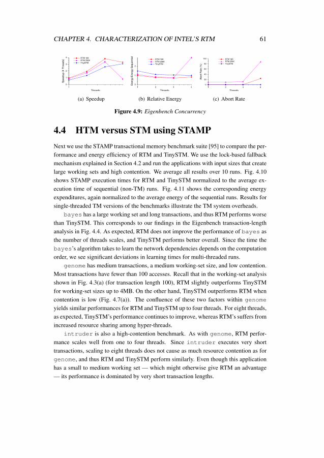
CHAPTER 4. CHARACTERIZATION OF INTEL’S RTM 61
1
Threads
0
1
2
3
4
Sp
ee
du
p (
4 T
hre
ad
s)
RTM 16K
RTM 256K
TinySTM
(a) Speedup
1 2 4 81
Threads
0
1
2
En
erg
y/E
ne
rgy-S
eq
ue
ntia
l
RTM 16K
RTM 256K
TinySTM
(b) Relative Energy
1 2 4 81
Threads
0
20
40
60
80
100
Ab
ort
Ra
te (
%)
RTM 16K
RTM 256K
TinySTM
(c) Abort Rate
Figure 4.9: Eigenbench Concurrency
4.4 HTM versus STM using STAMPNext we use the STAMP transactional memory benchmark suite [95] to compare the per-formance and energy efficiency of RTM and TinySTM. We use the lock-based fallbackmechanism explained in Section 4.2 and run the applications with input sizes that createlarge working sets and high contention. We average all results over 10 runs. Fig. 4.10shows STAMP execution times for RTM and TinySTM normalized to the average ex-ecution time of sequential (non-TM) runs. Fig. 4.11 shows the corresponding energyexpenditures, again normalized to the average energy of the sequential runs. Results forsingle-threaded TM versions of the benchmarks illustrate the TM system overheads.
bayes has a large working set and long transactions, and thus RTM performs worsethan TinySTM. This corresponds to our findings in the Eigenbench transaction-lengthanalysis in Fig. 4.4. As expected, RTM does not improve the performance of bayes asthe number of threads scales, and TinySTM performs better overall. Since the time thebayes’s algorithm takes to learn the network dependencies depends on the computationorder, we see significant deviations in learning times for multi-threaded runs.
genome has medium transactions, a medium working-set size, and low contention.Most transactions have fewer than 100 accesses. Recall that in the working-set analysisshown in Fig. 4.3(a) (for transaction length 100), RTM slightly outperforms TinySTMfor working-set sizes up to 4MB. On the other hand, TinySTM outperforms RTM whencontention is low (Fig. 4.7(a)). The confluence of these two factors within genome
yields similar performances for RTM and TinySTM up to four threads. For eight threads,as expected, TinySTM’s performance continues to improve, whereas RTM’s suffers fromincreased resource sharing among hyper-threads.
intruder is also a high-contention benchmark. As with genome, RTM perfor-mance scales well from one to four threads. Since intruder executes very shorttransactions, scaling to eight threads does not cause as much resource contention as forgenome, and thus RTM and TinySTM perform similarly. Even though this applicationhas a small to medium working set — which might otherwise give RTM an advantage— its performance is dominated by very short transaction lengths.

CHAPTER 4. CHARACTERIZATION OF INTEL’S RTM 62
kmeans is a clustering algorithm that groups data items in N-dimensional space intoK clusters. As with bayes, our 10 runtimes deviate significantly for the multi-threadedversions. On average, RTM performs better than TinySTM. The short transactions ex-perience low contention, and the small working set has high locality, all of which giveRTM a performance advantage over TinySTM. Even though both TM systems showspeedups over the sequential runs, synchronizing the kmeans algorithm in TinySTMexpends more energy at all thread counts.
labyrinth routes a path in a three-dimensional maze, where each thread grabs astart and an end point and connects them through adjacent grid points. Fig. 4.10 showsthat labyrinth does not scale in RTM. This is because each thread makes a copy of theglobal grid inside the transaction, triggering capacity aborts that eventually cause thefallback to using a lock. Energy expenditure increases for the RTM multi-threaded runsbecause the threads try to execute the transaction in parallel but eventually fail, wastingmany instructions while increasing cache and bus activity.
ssca2 has short transactions, a small read-write set, and low contention, and thuseven though it has a large working set, it scales well to higher thread counts. Performancefor eight threads is good for both RTM and TinySTM. In general, RTM performs better(with respect to both execution time and energy expenditure) but not by much, as is tobe expected for very short transactions.
vacation has low to medium contention among threads and a medium working setsize. The transactions are of medium length, locality is medium, and contention is low.Like genome, vacation scales well up to four threads, but performance degrades foreight threads because its read-write set size is large enough that cache sharing causesresource limitation issues.
yada has big working set, medium transaction length, large read-write set, andmedium contention. All these conditions give TinySTM a consistent performance ad-vantage over RTM at all thread counts.
Our results in Fig. 4.11 indicate that the energy trends of applications do not alwaysfollow their performance trends. Applications like bayes, labyrinth, and yada
expend more energy as they are scaled up, even when performance changes little (oreven improves, in the case of yada). Only intruder, kmeans, and ssca2 benefitfrom hyper-threading under RTM. In contrast, most STAMP applications benefit fromhyper-threading under TinySTM, and those that do not suffer only small degradations.
Fig. 4.12 shows the overall abort rates for all benchmarks, including the contribu-tions of different abort types. Based on our observations of hardware counter values,the current RTM implementation does not seem to distinguish between data-conflictaborts and aborts caused by read-set evictions from L3 cache, and thus both phenomenaare reported as conflict aborts. When a thread incurs the maximum number of failed

CHAPTER 4. CHARACTERIZATION OF INTEL’S RTM 63
1 2
bayes
4 8 1 2
genome
4 8 1 2
intruder
4 8 1 2
kmeans
4 8 1 2
labyrinth
4 8 1 2
ssca2
4 8 1 2
vacation
4 8 1 2
yada
4 8threads:0
1
2
Norm
aliz
ed e
xecution tim
e
(low
er
is b
etter)
RTM
TinySTM
Figure 4.10: RTM versus TinySTM Performance for STAMP Benchmarks
1 2
bayes
4 8 1 2
genome
4 8 1 2
intruder
4 8 1 2
kmeans
4 8 1 2
labyrinth
4 8 1 2
ssca2
4 8 1 2
vacation
4 8 1 2
yada
4 8threads:0
1
2
3
Norm
aliz
ed e
nerg
y e
xpenditure
(low
er
is b
etter)
RTM
TinySTM
Figure 4.11: RTM versus TinySTM Energy Expenditure for STAMP Benchmarks
transactions and acquires the lock in the fallback path, it forces all currently runningtransactions to abort. We term this a lock abort. These aborts are reported either as con-flict aborts, explicit aborts (i.e., deliberately triggered by the application code), or both(i.e., the machine increments multiple counters). Lock aborts are specific to the fallbackmechanism we use in our experiments. Other fallback mechanisms that do not use se-rialization locks within transactions (they can be employed in non-transactional code)do not incur such aborts. Note that avoiding lock aborts does not necessarily result inbetter performance since the lock aborts mask other type of aborts (i.e., that would haveoccurred subsequently). This can be seen in abort contributions shown in the figure. Asapplications are scaled, the fraction of aborts caused by locks increases because everyacquisition potentially triggers N -1 lock aborts (where N is the number of threads).
The RTM_RETIRED:ABORTED_MISC3 performance counter reports aborts dueto events like issuing unsupported instructions, page faults, and page table modifica-tions. The RTM_RETIRED:ABORTED_MISC5 counter includes miscellaneous abortsnot categorized elsewhere, such as aborts caused by interrupts. Table 4.3 gives anoverview of these abort types. In addition to these counters, three more performancecounters represent categorized abort numbers: RTM_RETIRED:ABORTED_MISC1 countsaborts due to memory events like data conflicts and capacity overflows; RTM_RETIRED:ABORTED_MISC2 counts aborts due to uncommon conditions; and RTM_RETIRED:ABORTED_MISC4 counts aborts due to incompatible memory types (e.g., due to cachebypassing or I/O accesses). In our experiments, RTM_RETIRED:ABORTED_MISC4counts are always less than 20, which we attribute to hardware error (as per the Intelspecification update [98]). In all our experiments, RTM_RETIRED:ABORTED_MISC2is zero.

CHAPTER 4. CHARACTERIZATION OF INTEL’S RTM 64
Abort Type Description
Data-conflict/Read-capacity
Conflict aborts and read-set capacity aborts
Write-capacity Write-set capacity abortsLock Conflict and explicit aborts caused by serialization locksMisc3 Unsupported instruction abortsa
Misc5 Aborts due to none of the previous categoriesb
a includes explicit aborts and aborts due to page fault/page table modificationb interrupts, etc.
Table 4.3: Intel RTM Abort Types
Figure 4.12: RTM Abort Distributions for STAMP Benchmarks
4.5 Related WorkHardware transactional memory systems must track memory updates within transac-tions and detect conflicts (read-write, write-read, or write-write conflicts across concur-rent transactions or non-transactional writes to active locations within transactions) atthe time of access. The choice of where to buffer speculative memory modificationshas microarchitectural ramifications, and commercial implementations naturally striveto minimize modifications to the the cores and on-chip memory hierarchies on whichthey are based. For instance, Blue Gene/Q [92] tracks updates in the 32MB L2 cache,and the IBM System z [93] series and the canceled Sun Rock [90] track updates in theirstore queues. Like the Haswell RTM implementation that we study here, the Vega AzulJava compute appliance [91] uses the L1 cache to record speculative writes. The size oftransactions that can benefit from such hardware TM support depends on the capacity ofthe chosen buffering scheme. Like us, others have found that rewriting software to bemore transaction-friendly improves hardware TM effectiveness [91].
Previous studies investigate the characteristics of hardware transactional memorysystems. Wang et al. [92] use the STAMP benchmarks to evaluate hardware transactionalmemory support on Blue Gene/Q, finding that the largest source of TM overhead is lossof cache locality from bypassing or flushing the L1 cache.

CHAPTER 4. CHARACTERIZATION OF INTEL’S RTM 65
Yoo et al. [94] use the STAMP benchmarks to compare Haswell RTM with the TL2software transactional memory system [99], finding significant performance differencesbetween TL2 and RTM. We perform a similar study and find that TinySTM consistentlyoutperforms TL2, and thus we choose the former as our STM point of comparison. OurRTM scaling results for STAMP benchmark concur with their results.
Wang et al. [100] evaluate RTM performance for concurrent skip list scalability,comparing against competing synchronization mechanisms like fine-grained locking andlock-free linked-lists. They use the Intel RTM emulator to model up to 40 cores, corrob-orating results for one to eight cores with Haswell hardware experiments. Like us, theyhighlight RTM performance limitations due to capacity and conflict misses and proposeprogrammer actions that can improve RTM performance.
Others have also studied power/performance trade-offs for TM systems. For in-stance, Gaona et al. [101] perform a simulation-based energy characterization study oftwo HTM systems: the LogTM-SE Eager-Eager system [86] and the Scalable TCCLazy-Lazy system [102]. Ferri et al. [103] estimate the performance and energy implica-tions of using TM in an embedded multiprocessor system-on-chips (MPSoCs), providingdetailed energy distribution figures from their energy models.
In contrast to the work presented here, none of these studies analyzes energy expen-diture for a commercial hardware implementation.
4.6 ConclusionsThe Restricted Transactional Memory support available in the Intel Haswell microar-chitecture makes programming with transactions more accessible to parallel computingresearchers and practitioners. In this study, we compare RTM and TinySTM, a soft-ware transactional memory implementation, in terms of performance and energy. Wehighlight RTM’s hardware limitations and quantify their effects on application behavior,finding that performance degrades for workloads with large working sets and long trans-actions. Enabling hyper-threading worsens RTM performance due to resource sharing atthe L1 level. We give details about the sources of aborts in a TM application and a way toquantiy these aborts. Using the knowledge presented in this thesis, parallel programmerscan optimize TM applications to better utilize the Haswell support for RTM.

5Conclusion
The significance of power-aware computing technologies is rapidly increasing becauseof the expanding carbon footprint of ICT sector. Analyzing the power consumptionof a system is a fundamental step in formulating power-aware techniques. This thesisproposes methodologies to better enable power-aware research through power measure-ment, power modeling, and power characterization.
5.1 ContributionsThis thesis makes following contributions:
Power Measurement (Chapter 2). We develop an infrastructure to measure power con-sumption at three points in voltage supply path of the processor: at the wall out-let, at the ATX power rails and at the CPU voltage regulator. We do a qualitativecomparison for the measurements sampled from the three points for accuracy andsensitivity. We discuss the advantages and disadvantages of each sampling point.We show that sampling power at the wall outlet is easiest but also least accurate.We test Intel’s digital power model (available to the software through RunningAverage Power Limit (RAPL) interface) for accuracy, overhead and temporal
66

CHAPTER 5. CONCLUSION 67
granularity. We demonstrate that the RAPL model estimates power with goodmean accuracy but suffers with infrequent high deviations from the mean.
Power Modeling (Chapter 3). We build upon the power model developed by Singh etal. [16, 63] that estimates power consumption of individual cores in chip mul-tiprocessors. We port and validate the model across many platforms, improvemodel accuracy by augmenting microbenchmark and counter selection method-ology, provide analysis for model estimation errors, and show the effectiveness ofthe model for the meta-scheduler that uses multiple DVFS operating points andprocess suspension to enforce power budget.
Characterization of Intel’s Restricted Transactional Memory (Chapter 4). We presenta detailed evaluation of Intel’s Restricted Transactional Memory (RTM) perfor-mance and energy expenditure. We compare RTM behavior to that of the TinySTMsoftware transactional memory system, first by running microbenchmarks, andthen by running the STAMP benchmark suite. We quantify the RTM hardwarelimitations concerning its read/write-set size, duration and overhead. We find thatRTM performs well when transaction working-set fits inside cache. RTM alsohandles high contention workloads better than TinySTM.
5.2 Future WorkThe methodologies presented in this thesis give rise to many future research directions.
The RTM characterization we presented in Chapter 4 is an initial study. We plan toexpand this study by exploring techniques to perform energy profiling for transactionalbenchmarks to help the programmers who will like to do energy-aware code optimiza-tions. The orthogonal characterization used in our work is useful in visualizing theeffects of an individual transactional property on the energy expenditure of the system.However, hybrid transactional memory schemes that use both hardware and softwaretransactional memory would need to evaluate all the transactional properties simulta-neously, which will be difficult because of huge number of operating points involved.We plan to explore machine learning techniques for helping such hybrid TM schemes inmaking an HTM versus STM decision.
The STAMP results in Chapter 4 show that energy consumption of benchmarks withlarge working sets increases even when the performance remains the same or decreases.We intend to explore this further and devise remedial measures, if possible.
Datacenters are major power consumers in the ICT sector and present many op-portunities in power-aware computing. We plan to expand our power modeling andcharacterization approaches to datacenter workloads and explore how datacenter spe-

CHAPTER 5. CONCLUSION 68
cific characteristics like data replication, data placement, and data volumes affect overallenergy expenditure.

Bibliography
[1] The Climate Group, “SMART 2020 : Enabling the Low Carbon Economy in theInformation Age,” GeSI’s Activity Report, The Climate Group on behalf of theGlobal eSustainability Initiative (GeSI), June 2008.
[2] Ryan Heath and Linda Cain, “Digital Agenda: global tech sector measuresits carbon footprint,” http://europa.eu/rapid/press-release_
IP-13-231_en.htm, 2013.
[3] S. Murugesan, “Harnessing green it: Principles and practices,” IEEE IT Profes-sional, vol. 10, no. 1, pp. 24–33, 2008.
[4] Gary Cook and Jodie Van Horn, “How Dirty is your Data,” A Look at the EnergyChoices That Power Cloud Computing, 2011.
[5] Parthasarathy Ranganathan, “Recipe for efficiency: principles of power-awarecomputing,” Communications of the ACM, vol. 53, no. 4, pp. 60–67, 2010.
[6] E. Rotem, A. Naveh, D. Rajwan, A. Ananthadrishnan, and E Weissmann, “Powermanagement architecture of the 2nd generation Intel R© CoreTM microarchitecture,formerly codenamed Sandy Bridge,” in Proc. 23rd HotChips Symposium on HighPerformance Chips, August 2011.
[7] Advanced Micro Devices, “AMD OpteronTM 6200 series processors linux tun-ing guide,” 2012, http://developer.amd.com/wordpress/media/
2012/10/51803A_OpteronLinuxTuningGuide_SCREEN.pdf.
[8] NVIDIA, Nvidia NVML API Reference Manual, 2012.
[9] Abhinav Pathak, Y Charlie Hu, Ming Zhang, Paramvir Bahl, and Yi-Min Wang,“Fine-grained power modeling for smartphones using system call tracing,” inProc. the sixth conference on Computer systems. ACM, 2011, pp. 153–168.
[10] R. Joseph and M. Martonosi, “Run-time power estimation in high-performancemicroprocessors,” in Proc. IEEE/ACM International Symposium on Low PowerElectronics and Design, August 2001, pp. 135–140.
69

BIBLIOGRAPHY 70
[11] K. Rajamani, H. Hanson, J. Rubio, S. Ghiasi, and F. Rawson, “Application-awarepower management,” in Proc. IEEE International Symposium on PerformanceAnalysis of Systems and Software, October 2006, pp. 39–48.
[12] F. Bellosa, S. Kellner, M. Waitz, and A. Weissel, “Event-driven energy accountingfor dynamic thermal management,” in Proc. of the Workshop on Compilers andOperating Systems for Low Power (COLP’03), Sept. 2003.
[13] R. Bertran, M. Gonzalez, X. Martorell, N. Navarro, and E. Ayguade, “Decom-posable and responsive power models for multicore processors using performancecounters,” in Proc. 24th ACM International Conference on Supercomputing, June2010, pp. 147–158.
[14] G. Contreras and M. Martonosi, “Power prediction for Intel XScale processorsusing performance monitoring unit events,” in Proc. IEEE/ACM InternationalSymposium on Low Power Electronics and Design, August 2005, pp. 221–226.
[15] D. Economou, S. Rivoire, C. Kozyrakis, and P. Ranganathan, “Full-system poweranalysis and modeling for server environments,” in Proc. Workshop on Modeling,Benchmarking, and Simulation, June 2006.
[16] K. Singh, M. Bhadauria, and S.A. McKee, “Real time power estimation andthread scheduling via performance counters,” November 2008.
[17] R Ren, E Juarez, C Sanz, Mickael Raulet, and F Pescador, “System-level PMC-driven energy estimation models in RVC-CAL video codec specifications,” inProc. Conference on Design and Architectures for Signal and Image Processing(DASIP). IEEE, 2013, pp. 55–62.
[18] B.C. Lee and D.M. Brooks, “Accurate and efficient regression modeling for mi-croarchitectural performance and power prediction,” in Proc. 12th ACM Sympo-sium on Architectural Support for Programming Languages and Operating Sys-tems, October 2006, pp. 185–194.
[19] Krishna Rangan, Gu-Yeon Wei, and David Brooks, “Thread motion: Fine-grainedpower management for multi-core systems,” in Proc. 36th IEEE/ACM Interna-tional Symposium on Computer Architecture, June 2009.
[20] M. Banikazemi, D. Poff, and B. Abali, “PAM: A novel performance/power awaremeta-scheduler for multi-core systems,” in Proc. IEEE/ACM SupercomputingInternational Conference on High Performance Computing, Networking, Storageand Analysis, November 2008, number 39.
[21] C. Isci, A. Buyuktosunoglu, C.Y. Cher, P. Bose, and M. Martonosi, “An analysisof efficient multi-core global power management policies: Maximizing perfor-mance for a given power budget,” in Proc. IEEE/ACM 40th Annual InternationalSymposium on Microarchitecture, December 2006, pp. 347–358.

BIBLIOGRAPHY 71
[22] Ke Meng, Russ Joseph, Robert P. Dick, and Li Shang, “Multi-optimization powermanagement for chip multiprocessors,” in Proc. the 17th international conferenceon Parallel architectures and compilation techniques, 2008, pp. 177–186.
[23] V. Spiliopoulos, S. Kaxiras, and G. Keramidas, “Green governors: A frame-work for continuously adaptive dvfs,” in Proc. Green Computing Conference andWorkshops (IGCC), 2011 International, July 2011, pp. 1–8.
[24] Kyong Hoon Kim, Rajkumar Buyya, and Jong Kim, “Power aware scheduling ofbag-of-tasks applications with deadline constraints on DVS-enabled Clusters,” inCCGRID, 2007, vol. 7, pp. 541–548.
[25] Josep Ll Berral, Íñigo Goiri, Ramón Nou, Ferran Julià, Jordi Guitart, RicardGavaldà, and Jordi Torres, “Towards energy-aware scheduling in data centersusing machine learning,” in Proc. the 1st International Conference on energy-Efficient Computing and Networking. ACM, 2010, pp. 215–224.
[26] Gregor Von Laszewski, Lizhe Wang, Andrew J Younge, and Xi He, “Power-awarescheduling of virtual machines in dvfs-enabled clusters,” in Cluster Computingand Workshops, 2009. CLUSTER’09. IEEE International Conference on. IEEE,2009, pp. 1–10.
[27] Tridib Mukherjee, Ayan Banerjee, Georgios Varsamopoulos, Sandeep KS Gupta,and Sanjay Rungta, “Spatio-temporal thermal-aware job scheduling to minimizeenergy consumption in virtualized heterogeneous data centers,” Computer Net-works, vol. 53, no. 17, pp. 2888–2904, 2009.
[28] Qinghui Tang, Sandeep KS Gupta, and Georgios Varsamopoulos, “Energy-efficient thermal-aware task scheduling for homogeneous high-performance com-puting data centers: A cyber-physical approach,” IEEE Transactions on Paralleland Distributed Systems, vol. 19, no. 11, pp. 1458–1472, 2008.
[29] Xin Zhan and Sherief Reda, “Techniques for energy-efficient power budgeting indata centers,” in Proc. the 50th Annual Design Automation Conference, 2013, pp.176:1–176:7.
[30] Victor Jimenez, Francisco Cazorla, Roberto Gioiosa, Eren Kursun, Canturk Isci,Alper Buyuktosunoglu, Pradip Bose, and Mateo Valero, “Energy-aware account-ing and billing in large-scale computing facilities,” IEEE Micro, vol. 31, no. 3,pp. 60–71, 2011.
[31] Jeonghwan Choi, Chen-Yong Cher, Hubertus Franke, Henrdrik Hamann, AlanWeger, and Pradip Bose, “Thermal-aware task scheduling at the system softwarelevel,” in Proc. the 2007 international symposium on Low power electronics anddesign. ACM, 2007, pp. 213–218.

BIBLIOGRAPHY 72
[32] Ayse Kivilcim Coskun, Tajana Simunic Rosing, and Keith Whisnant, “Temper-ature aware task scheduling in mpsocs,” in Proc. the conference on Design, au-tomation and test in Europe. EDA Consortium, 2007, pp. 1659–1664.
[33] Abhinav Pathak, Y. Charlie Hu, and Ming Zhang, “Where is the energy spentinside my app?: Fine grained energy accounting on smartphones with eprof,” inProc. the 7th ACM European Conference on Computer Systems, 2012, EuroSys’12, pp. 29–42.
[34] K.S. Banerjee and E. Agu, “PowerSpy: fine-grained software energy profiling formobile devices,” in Proc. 2005 International Conference on Wireless Networks,Communications and Mobile Computing, 2005, vol. 2, pp. 1136–1141 vol.2.
[35] J. Flinn and M. Satyanarayanan, “Powerscope: A tool for profiling the energyusage of mobile applications,” in Proc. 2nd IEEE Workshop on Mobile ComputingSystems and Applications, February 1999, pp. 2–10.
[36] Y.S. Shao and D. Brooks, “Energy characterization and instruction-level energymodel of intel’s xeon phi processor,” in Proc. 2013 IEEE International Sympo-sium on Low Power Electronics and Design (ISLPED), 2013, pp. 389–394.
[37] Ramon Bertran, Alper Buyuktosunoglu, Meeta S. Gupta, Marc Gonzalez, andPradip Bose, “Systematic energy characterization of CMP/SMT processorsystems via automated micro-benchmarks,” in Proc. the 2012 45th AnnualIEEE/ACM International Symposium on Microarchitecture, Washington, DC,USA, 2012, MICRO-45, pp. 199–211, IEEE Computer Society.
[38] T. Mukherjee, G. Varsamopoulos, S. K S Gupta, and S. Rungta, “Measurement-based power profiling of data center equipment,” in 2007 IEEE InternationalConference on Cluster Computing, 2007, pp. 476–477.
[39] Epifanio Gaona, Rubén Titos-Gil, Juan Fernandez, and Manuel E. Acacio, “Char-acterizing energy consumption in hardware transactional memory systems,” inProc. 22nd International Symposium on Computer Architecture and High Perfor-mance Computing (SBAC-PAD), 2010, pp. 9–16.
[40] Y. Guo, S. Chheda, I. Koren, C. M. Krishna, and C. A. Moritz, “Energy Char-acterization of Hardware-Based Data Prefetching,” in Proc. IEEE InternationalConference on Computer Design, 2004, pp. 518–523.
[41] Marc Gamell, Ivan Rodero, Manish Parashar, Janine C. Bennett, Hemanth Kolla,Jacqueline Chen, Peer-Timo Bremer, Aaditya G. Landge, Attila Gyulassy, PatrickMcCormick, Scott Pakin, Valerio Pascucci, and Scott Klasky, “Exploring powerbehaviors and trade-offs of in-situ data analytics,” in Proc. SC13: InternationalConference for High Performance Computing, Networking, Storage and Analysis,2013, SC ’13, pp. 77:1–77:12.
BIBLIOGRAPHY 73
[42] John C. McCullough, Yuvraj Agarwal, Jaideep Chandrashekar, SathyanarayanKuppuswamy, Alex C. Snoeren, and Rajesh K. Gupta, “Evaluating the effective-ness of model-based power characterization,” in Proc. the 2011 USENIX Confer-ence on USENIX Annual Technical Conference, 2011, pp. 12–12.
[43] B. Goel, S.A. McKee, R. Gioiosa, K. Singh, M. Bhadauria, and M. Cesati,“Portable, scalable, per-core power estimation for intelligent resource manage-ment,” in Proc. 1st International Green Computing Conference, August 2010,pp. 135–146.
[44] C. Sun, L. Shang, and R.P. Dick, “Three-dimensional multiprocessor system-on-chip thermal optimization,” in Proc. 5th IEEE/ACM international conference onHardware/software codesign and system synthesis, 2007, pp. 117–122.
[45] E. Stahl, “Power Benchmarking: A new methodology for analyzing performanceby applying energy efficiency metrics,” White Paper, IBM, 2006.
[46] Standard Performance Evaluation Corporation, “SPECpower_ssj2008 benchmarksuite,” http://www.spec.org/power_ssj2008/, 2008.
[47] B. Goel, R. Titos-Gil, A. Negi, S.A. McKee, and P. Stenstrom, “Performanceand energy analysis of the restricted transactional memory implementation onhaswell,” in Proceedings of the Proc. International Parallel and Distributed Pro-cessing Symposium, 2014, To appear.
[48] Marcus Hähnel, Björn Döbel, Marcus Völp, and Hermann Härtig, “Measuringenergy consumption for short code paths using RAPL,” SIGMETRICS Perform.Eval. Rev., vol. 40, no. 3, pp. 13–17, January 2012.
[49] Electronic Educational Devices, “Watts Up PRO,” http://www.
wattsupmeters.com/, May 2009.
[50] X. Wang and M. Chen, “Cluster-level feedback power control for performanceoptimization,” in Proc. 14th IEEE International Symposium on High PerformanceComputer Architecture, February 2008, pp. 101–110.
[51] D. Bedard, M. Y. Lim, R. Fowler, and A. Porterfield, “Powermon: Fine-grainedand integrated power monitoring for commodity computer systems,” in Proc.IEEE SoutheastCon 2010 (SoutheastCon), Mar. 2010, pp. 479–484.
[52] Server System Infrastructure Forum, EPS12V Power Supply Design Guide, Dell,HP, SGI, and IBM, 2.92 edition, 2006.
[53] LEM Corporation, “Intel current transducer LTS 25-NP,” Datasheet, LEM,November 2009.

BIBLIOGRAPHY 74
[54] National Instruments Corporation, “NI bus-powered m series multifunction daqfor usb,” http://sine.ni.com/ds/app/doc/p/id/ds-9/lang/en,Apr. 2009.
[55] Intel Corporation, “Voltage regulator-down (VRD) 11.1,” Design Guidelines,Intel Corporation, Sept. 2009.
[56] Intel, Intel Architecture Software Developer’s Manual: System ProgrammingGuide, June 2013.
[57] D. Hackenberg, T. Ilsche, R. Schone, D. Molka, M. Schmidt, and W.E. Nagel,“Power measurement techniques on standard compute nodes: A quantitative com-parison,” in Proc. 2013 IEEE International Symposium on Performance Analysisof Systems and Software (ISPASS), 2013, pp. 194–204.
[58] C. Isci and M. Martonosi, “Runtime power monitoring in high-end processors:Methodology and empirical data,” in Proc. IEEE/ACM 37th Annual InternationalSymposium on Microarchitecture, 2003, pp. 93–104.
[59] Z. Cui, Y. Zhu, Y. Bao, and M. Chen, “A fine-grained component-level powermeasurement method,” in Proc. 2nd International Green Computing Conference,July 2011, pp. 1–6.
[60] Intel Corporation, “Intel CoreTM i7 Processor,” http://www.intel.com/products/processor/corei7/, December 2008.
[61] M.S. Floyd, S. Ghiasi, T.W. Keller, K. Rajamani, F.L. Rawson, J.C. Rubio, andM.S. Ware, “System power management support in the IBM POWER6 micropro-cessor,” IBM Journal of Research and Development, vol. 51, no. 6, pp. 733–746,2007.
[62] H.-Y. McCreary, M.A. Broyles, M.S. Floyd, A.J. Geissler, S.P. Hartman, F.L.Rawson, T.J. Rosedahl, J.C. Rubio, and M.S. Ware, “Energyscale for IBMPOWER6 microprocessor-based systems,” IBM Journal of Research and De-velopment, vol. 51, no. 6, pp. 775–786, 2007.
[63] K. Singh, Prediction Strategies for Power-Aware Computing on Multicore Pro-cessors, Ph.D. thesis, Cornell University, 2009.
[64] V.M. Weaver and S.A. McKee, “Can hardware performance counters be trusted?,”in Proc. IEEE International Symposium on Workload Characterization, Sept.2008, pp. 141–150.
[65] D. Zaparanuks, M. Jovic, and M. Hauswirth, “Accuracy of performance countermeasurements,” Tech. Rep. USI-TR-2008-05, Università della Svizzera italiana,Sept. 2008.

BIBLIOGRAPHY 75
[66] V.M. Weaver and J. Dongarra, “Can hardware performance counters produceexpected, deterministic results,” in In Proc. 3rd Workshop on Functionality ofHardware Performance Monitoring, December 2010.
[67] Intel, Intel 64 and IA-32 Architectures Software Developer’s Manual, May 2013.
[68] N.S. Kim, T. Austin, D. Baauw, T. Mudge, K. Flautner, J.S. Hu, M.J. Irwin,M. Kandemir, and V. Narayanan, “Leakage current: Moore’s law meets staticpower,” IEEE Computer, vol. 36, no. 12, pp. 68–75, December 2003.
[69] M. Berktold and T. Tian, “CPU monitoring with DTS/PECI,” White Paper,Intel Corporation. http://download.intel.com/design/intarch/papers/322683.pdf, Sept. 2010.
[70] C. Spearman, “The proof and measurement of association between two things,”The American Journal of Psychology, vol. 15, no. 1, pp. 72–101, January 1904.
[71] Standard Performance Evaluation Corporation, “SPEC CPU benchmark suite,”http://www.specbench.org/osg/cpu2006/, 2006.
[72] Standard Performance Evaluation Corporation, “SPEC OMP benchmark suite,”http://www.specbench.org/hpg/omp2001/, 2001.
[73] V. Aslot and R. Eigenmann, “Performance characteristics of the SPEC OMP2001benchmarks,” in Proc. European Workshop on OpenMP, Sept. 2001.
[74] D.H. Bailey, T. Harris, W.C. Saphir, R.F. Van der Wijngaart, A.C. Woo, andM. Yarrow, “The NAS parallel benchmarks 2.0,” Report NAS-95-020, NASAAmes Research Center, December 1995.
[75] S. Eranian, “Perfmon2: A flexible performance monitoring interface for Linux,”in Proc. 2006 Ottawa Linux Symposium, July 2006, pp. 269–288.
[76] C. Boneti, R. Gioiosa, F.J. Cazorla, and M. Valero, “A dynamic scheduler forbalancing HPC applications,” in Proc. IEEE/ACM Supercomputing InternationalConference on High Performance Computing, Networking, Storage and Analysis,November 2008, number 41.
[77] E. Betti, M. Cesati, R. Gioiosa, and F. Piermaria, “A global operating system forHPC clusters,” in Proc. IEEE International Conference on Cluster Computing,August 2009, p. 6.
[78] Advanced Micro Devices, AMD Athlon Processor Model 6 Revision Guide, 2003.
[79] T. Austin, “SimpleScalar 4.0 release note,” http://www.simplescalar.com/.

BIBLIOGRAPHY 76
[80] W. Wu, L. Jin, and J. Yang, “A systematic method for functional unit powerestimation in microprocessors,” in Proc. 43rd ACM/IEEE Design AutomationConference, July 2006, pp. 554–557.
[81] A. Merkel and F. Bellosa, “Balancing power consumption in multicore proces-sors,” in Proc. ACM SIGOPS/EuroSys European Conference on Computer Sys-tems, Apr. 2006, pp. 403–414.
[82] E. Grochowski, R. Ronen, J. Shen, and H. Wang, “Best of both latency andthroughput,” in Proc. IEEE International Conference on Computer Design, Oc-tober 2004, pp. 236–243.
[83] M. Annavaram, E. Grochowski, and J. Shen, “Mitigating Amdahl’s Law throughEPI throttling,” in Proc. 32nd IEEE/ACM International Symposium on ComputerArchitecture, June 2005, pp. 298–309.
[84] M. Moudgill, P. Bose, and J. Moreno, “Validation of Turandot, a fast processormodel for microarchitecture exploration,” in Proc. International Performance,Computing, and Communications Conference, February 1999, pp. 452–457.
[85] Maurice Herlihy and J. Eliot B. Moss, “Transactional memory: Architecturalsupport for lock-free data structures,” in Proceedings of the 20th InternationalSymposium on Computer Architecture, 1993, pp. 289–300.
[86] Luke Yen, Jayaram Bobba, Michael R. Marty, Kevin E. Moore, Haris Volos,Mark D. Hill, Michael M. Swift, and David A. Wood, “LogTM-SE: Decou-pling hardware transactional memory from caches,” in Proceedings of the 13thSymposium on High-Performance Computer Architecture, 2007, pp. 261–272.
[87] Lance Hammond, Vicky Wong, Mike Chen, Brian D. Carlstrom, John D. Davis,Ben Hertzberg, Manohar K. Prabhu, Honggo Wijaya, Christos Kozyrakis, andKunle Olukotun, “Transactional memory coherence and consistency,” in Pro-ceedings of the 31st International Symposium on Computer Architecture, 2004,pp. 102–113.
[88] Marc Lupon, Grigorios Magklis, and Antonio González, “A dynamically adapt-able hardware transactional memory,” in Proceedings of the 43rd InternationalSymposium on Microarchitecture, 2010, pp. 27–38.
[89] Rubén Titos-Gil, Anurag Negi, Manuel E. Acacio, Jose M. Garcia, and Per Sten-strom, “Zebra : A data-centric, hybrid-policy hardware transactional memorydesign,” in Proceedings of the 25th International Conference of Supercomputing,2011, pp. 53–62.
[90] Dave Dice, Yossi Lev, Mark Moir, and Daniel Nussbaum, “Early experience witha commercial hardware transactional memory implementation,” ACM SIGPLANNotices, vol. 44, no. 3, pp. 157–168, Mar. 2009.

BIBLIOGRAPHY 77
[91] Cliff Click, “Azul’s experiences with hardware transactional memory,” 2009,http://sss.cs.purdue.edu/projects/tm/tmw2010/talks/Click-2010_TMW.pdf.
[92] Amy Wang, Matthew Gaudet, Peng Wu, Jose Nelson Amaral, Martin Ohmacht,Christopher Barton, Raul Silvera, and Maged Michael, “Evaluation of BlueGene/Q hardware support for transactional memories,” in Proc. the 21st Interna-tional Conference on Parallel Architectures and Compilation Techniques, 2012,pp. 127–136.
[93] Christian Jacobi, Timothy Slegel, and Dan Greiner, “Transactional memory ar-chitecture and implementation for IBM System z,” in Proc. the 2012 45th AnnualIEEE/ACM International Symposium on Microarchitecture, 2012, pp. 25–36.
[94] Richard M. Yoo, Christopher J. Hughes, Konrad Lai, and Ravi Rajwar, “Per-formance evaluation of Intel transactional synchronization extensions for high-performance computing,” in Proc. SC13: International Conference for High Per-formance Computing, Networking, Storage and Analysis, 2013, pp. 19:1–19:11.
[95] Chi Cao Minh, JaeWoong Chung, Christos Kozyrakis, and Kunle Olukotun,“STAMP: Stanford transactional applications for multi-processing,” in Proceed-ings of the IEEE International Symposium on Workload Characterization, 2008,pp. 35–46.
[96] Sungpack Hong, Tayo Oguntebi, Jared Casper, Nathan Bronson, ChristosKozyrakis, and Kunle Olukotun, “Eigenbench: A simple exploration tool fororthogonal TM characteristics,” in Proc. the IEEE International Symposium onWorkload Characterization, 2010, pp. 1–11.
[97] Pascal Felber, Christof Fetzer, Patrick Marlier, and Torvald Riegel, “Time-basedsoftware transactional memory,” IEEE Transactions on Parallel and DistributedSystems, vol. 21, no. 12, pp. 1793–1807, 2010.
[98] Intel, Desktop 4th Generation Intel CoreTMProcessor Family Specification Up-date, August 2013.
[99] David Dice, Ori Shalev, and Nir Shavit, “Transactional Locking II,” in Proc. the19th International Symposium on Distributed Computing, 2006.
[100] Zhaoguo Wang, Hao Qian, Haibo Chen, and Jinyang Li, “Opportunities andpitfalls of multi-core scaling using hardware transaction memory,” in Proc. the4th Asia-Pacific Workshop on Systems, 2013, pp. 3:1–3:7.
[101] E. Gaona-Ramirez, R. Titos-Gil, J. Fernandez, and M.E. Acacio, “Characteriz-ing energy consumption in hardware transactional memory systems,” in Proc.22nd International Symposium on Computer Architecture and High PerformanceComputing (SBAC-PAD), 2010, pp. 9–16.
BIBLIOGRAPHY 78
[102] Hassan Chafi, Jared Casper, Brian D. Carlstrom, Austen McDonald, Chi CaoMinh, Woongki Baek, Christos Kozyrakis, and Kunle Olukotun, “A scalable,non-blocking approach to transactional memory,” in Proceedings of the 13thSymposium on High-Performance Computer Architecture, 2007, pp. 97–108.
[103] C. Ferri, R.I. Bahar, A. Marongiu, L. Benini, M. Herlihy, B. Lipton, and T. More-shet, “SoC-TM: Integrated HW/SW support for transactional memory program-ming on embedded MPSoCs,” in Proc. the 9th International Conference on Hard-ware/Software Codesign and System Synthesis, 2011, pp. 39–48.