measurement, modeling, and characterization for energy
TRANSCRIPT

THESIS FOR THE DEGREE OF DOCTOR OF PHILOSOPHY
Measurement, Modeling, andCharacterization for Energy-Efficient
Computing
BHAVISHYA GOEL
Division of Computer EngineeringDepartment of Computer Science and Engineering
CHALMERS UNIVERSITY OF TECHNOLOGY
Göteborg, Sweden 2016

Measurement, Modeling, and Characterization for Energy-Efficient ComputingBhavishya GoelISBN 978-91-7597-411-8
Copyright c© Bhavishya Goel, 2016.
Doktorsavhandlingar vid Chalmers tekniska högskolaNy serie Nr 4092ISSN 0346-718X
Technical Report 129DDepartment of Computer Science and EngineeringComputer Architecture Research Group
Department of Computer Science and EngineeringChalmers University of TechnologySE-412 96 GÖTEBORG, SwedenPhone: +46 (0)31-772 10 00
Author e-mail: [email protected]
Chalmers ReposerviceGöteborg, Sweden 2016

Measurement, Modeling, and Characterization for Energy-EfficientComputing
Bhavishya GoelDivision of Computer Engineering, Chalmers University of Technology
ABSTRACTThe ever-increasing ecological footprint of Information Technology (IT) sector coupledwith adverse effects of high power consumption on electronic circuits has increased thesignificance of energy-efficient computing in the last decade. Making energy-efficientcomputing a norm rather than an exception requires that system designers and program-mers understand the energy implications of their design and implementation choices.This necessitates a detailed view of system’s energy expenditure and/or power consump-tion. We explore this aspect of energy-efficient computing in this thesis through powermeasurement, power modeling, and energy characterization.
First, we present a quantitative comparison between power measurement data col-lected for computer systems using four techniques: a power meter at wall outlet, currenttransducers at ATX power rails, CPU voltage regulator’s current monitor, and Intel’sproprietary RAPL (Running Average Power Limit) interface. We compare them for ac-curacy, sensitivity and accessibility.
Second, we present two different methodologies to model processor power con-sumption. The first model estimates power consumption at the granularity of individ-ual cores using per-core performance events and temperature sensors. We validate themethodology on six different platforms and show that our model estimates power con-sumption with high accuracy across all platforms consistently. To understand the energyexpenditure trends across different frequencies and different degrees of parallelism, weneed to model power at a much finer granularity. The second power model addressesthis issue by estimating static and dynamic power consumption for individual cores andthe uncore. We validate this model on Intel’s Haswell platform for single-threaded andmulti-threaded benchmarks. We use this power model to characterize energy efficiencyof frequency scaling on Haswell microarchitecture and use the insights to implementa low overhead DVFS scheduler. We also characterize the energy efficiency of threadscaling using the power model and demonstrate how different communication parame-ters and microarchitectural traits affect application’s energy when it scales.
Finally, we perform detailed performance and energy characterization of Intel’s Re-stricted Transactional Memory (RTM). We use TinySTM software transactional memory(STM) system to benchmark RTM’s performance against competing STM alternatives.We use microbenchmarks and STAMP benchmark suite to compare RTM an STM per-formance and energy behavior. We quantify the RTM hardware limitations and identifyconditions required for RTM to outperform STM.
Keywords: power estimation, energy characterization, power-aware scheduling, power
management, transactional memory, power measurement

ii

Preface
Parts of the contributions presented in this thesis have previously been publishedin the following manuscripts.
. Bhavishya Goel, Sally A. McKee, Roberto Gioiosa, Karan Singh,Major Bhadauria, Marco Cesati, “Portable, Scalable, Per-Core PowerEstimation for Intelligent Resource Management” in Proceedingsof the 1st International Green Computing Conference, Chicago,USA, August, 2010, pp.135-146.
. Bhavishya Goel, Sally A. McKee, Magnus Själander, “Techniquesto Measure, Model, and Manage Power,” in Advances in Comput-ers 87, 2012, pp.7-54.
. Bhavishya Goel, Ruben Titos-Gil, Anurag Negi, Sally A. Mc-Kee, Per Stenstrom, “Performance and Energy Analysis of the Re-stricted Transactional Memory Implementation on Haswell” in Pro-ceedings of 28th IEEE International Parallel and Distributed Pro-cessing Symposium, Phoenix, USA, May, 2014, pp.615-624
The following manuscript has been accepted but is yet to be published.
. Bhavishya Goel, Sally A. McKee, “A Methodology for ModelingDynamic and Static Power Consumption for Multicore Processors”in Proceedings of 30th IEEE International Parallel and DistributedProcessing Symposium, Chicago, USA, May, 2016
The following manuscripts have been published but are not included in thiswork.
iii

PREFACE iv
. Bhavishya Goel, Magnus Själander, Sally A. McKee, “RTL Modelfor Dynamically Resizable L1 Data Cache” in Swedish System-on-Chip Conference, Ystad, Sweden, 2013
. Magnus Själander, Sally A. McKee, Bhavishya Goel, Peter Brauer,David Engdal, Andras Vajda, “Power-Aware Resource Schedulingin Base Stations” in 19th Annual IEEE/ACM International Sym-posium on Modeling, Analysis and Simulation of Computer andTelecommunication Systems, Singapore, Singapore, July, 2012, pp.462-465.

Acknowledgments
I will like to thank following people for supporting me during my PhD andcontributing to this thesis directly or indirectly.
. Professor Sally A. McKee for giving me the opportunity to work withher, for giving me the confidence boost during the lows and for cele-brating my highs. She always trusted me to choose my own researchpath but was always there whenever I needed her for counseling. She isalso an excellent cook and her brownies and palak paneers have got methrough various deadlines.
. Magnus Själander for helping me with my research during the earlyyears of my PhD and letting me bounce ideas off him. His unabatedenthusiasm for research is very contagious.
. Madhavan Manivannan for being a great friend and colleague; and forspending loads of his precious time to review my papers and thesis.
. Professor Lars Svensson for helping me with practical issues during histime as division head and for giving me critical feedback to improve thetechnical and non-technical aspects of this thesis.
. Professor Per Larsson-Edefors for teaching some of the most entertain-ing courses I have taken at Chalmers and for his valuable feedback fromtime to time.
. Professor Per Stenström for being an inspiration in the field of computerarchitecture.
. Professor Lieven Eeckhout for evaluating my licentiate thesis and forhis insightful comments on my research.
v

ACKNOWLEDGMENTS vi
. Anurag Negi for being an accommodating roommate and a helpful co-author.
. Ruben Titos for helping me in getting started with the basics of trans-actional memory, for doing his part in the paper we co-authored and forcheering me up with his positive vibes.
. Karan Singh, Vincent M. Weaver and Major Bhadauria for getting mestarted with the power modeling infrastructure at Cornell and answeringmy naïve questions patiently.
. Roberto Gioiosa and Marco Cesati for helping me run experiments formy first paper.
. Jacob Lidman for being an amazing study partner, for sharing officespace with me and putting up with my rants and bad jokes.
. Alen, Angelos, Bapi, Dmitry, Kasyab, Mafijul, Waliullah, Gabriele,Vinay, Jochen, Fatemeh, Behrooz, Chloe, Petros, Risat, Stavros, Alirad,Ahsen, Viktor, Miquel, Vassilis, Yiannis and Ivan for being wonderfulcolleagues and friends.
. Peter, Rune and Arne for proving invaluable IT support.
. Rolf Snedsböl for managing my teaching duties.
. Eva, Lotta, Tiina, Jonna, and Marianne for providing excellent adminis-trative support during my time at Chalmers.
. All the colleagues and staff at Computer Science and Engineering de-partment for creating a healthy work environment.
. Anthony Brandon for giving me valuable support when I was workingwith ρVEX processor for ERA project.
. European Union for funding my research.
. My family for motivating me to push for my goals and being there as abackup whenever I needed them.
Bhavishya GoelGöteborg, May 2016
Contents
Abstract i
Preface iii
Acknowledgments v
1 Introduction 21.1 Power Measurement . . . . . . . . . . . . . . . . . . . . . . . 81.2 Power Modeling . . . . . . . . . . . . . . . . . . . . . . . . . . 91.3 Energy Characterization . . . . . . . . . . . . . . . . . . . . . 101.4 Contributions . . . . . . . . . . . . . . . . . . . . . . . . . . . 101.5 Thesis Organization . . . . . . . . . . . . . . . . . . . . . . . . 12
2 Power Measurement Techniques 132.1 Power Measurement Techniques . . . . . . . . . . . . . . . . . 14
2.1.1 At the Wall Outlet . . . . . . . . . . . . . . . . . . . . 142.1.2 At the ATX Power Rails . . . . . . . . . . . . . . . . . 152.1.3 At the Processor Voltage Regulator . . . . . . . . . . . 172.1.4 Experimental Results . . . . . . . . . . . . . . . . . . . 19
2.2 RAPL power estimations . . . . . . . . . . . . . . . . . . . . . 242.2.1 Overview . . . . . . . . . . . . . . . . . . . . . . . . . 242.2.2 Experimental Results . . . . . . . . . . . . . . . . . . . 24
2.3 Related Work . . . . . . . . . . . . . . . . . . . . . . . . . . . 312.4 Conclusions . . . . . . . . . . . . . . . . . . . . . . . . . . . . 32
3 Per-core Power Estimation Model 333.1 Modeling Approach . . . . . . . . . . . . . . . . . . . . . . . . 37
vii

CONTENTS viii
3.2 Methodology . . . . . . . . . . . . . . . . . . . . . . . . . . . 383.2.1 Counter Selection . . . . . . . . . . . . . . . . . . . . . 383.2.2 Model Formation . . . . . . . . . . . . . . . . . . . . . 42
3.3 Validation . . . . . . . . . . . . . . . . . . . . . . . . . . . . . 443.3.1 Computation Overhead . . . . . . . . . . . . . . . . . . 463.3.2 Estimation Error . . . . . . . . . . . . . . . . . . . . . 46
3.4 Management . . . . . . . . . . . . . . . . . . . . . . . . . . . 533.4.1 Sample Policies . . . . . . . . . . . . . . . . . . . . . . 583.4.2 Experimental Setup . . . . . . . . . . . . . . . . . . . . 583.4.3 Results . . . . . . . . . . . . . . . . . . . . . . . . . . 60
3.5 Related Work . . . . . . . . . . . . . . . . . . . . . . . . . . . 623.6 Conclusions . . . . . . . . . . . . . . . . . . . . . . . . . . . . 65
4 Energy Characterization for Multicore Processors Using Dynamicand Static Power Models 674.1 Power Modeling Methodology . . . . . . . . . . . . . . . . . . 69
4.1.1 Uncore Dynamic Power Model . . . . . . . . . . . . . 694.1.2 Core Dynamic Power Model . . . . . . . . . . . . . . . 724.1.3 Uncore Static Power Model . . . . . . . . . . . . . . . 744.1.4 Core Static Power Model . . . . . . . . . . . . . . . . . 754.1.5 Total Chip Power Model . . . . . . . . . . . . . . . . . 77
4.2 Validation . . . . . . . . . . . . . . . . . . . . . . . . . . . . . 804.3 Energy Characterization of Frequency Scaling . . . . . . . . . . 81
4.3.1 Energy Effects of DVFS . . . . . . . . . . . . . . . . . 834.3.2 DVFS Prediction . . . . . . . . . . . . . . . . . . . . . 85
4.4 Energy Characterization of Thread Scaling . . . . . . . . . . . . 924.4.1 Energy Effects of Serial Fraction . . . . . . . . . . . . . 964.4.2 Energy Effects of Core-to-core Communication Overhead 994.4.3 Energy Effects of Bandwidth Contention . . . . . . . . 1024.4.4 Energy Effects of Locking-Mechanism Overhead . . . . 104
4.5 Related Work . . . . . . . . . . . . . . . . . . . . . . . . . . . 1064.6 Conclusions . . . . . . . . . . . . . . . . . . . . . . . . . . . . 108
5 Characterization of Intel’s Restricted Transactional Memory 1095.1 Experimental Setup . . . . . . . . . . . . . . . . . . . . . . . . 1105.2 Microbenchmark analysis . . . . . . . . . . . . . . . . . . . . . 112

CONTENTS ix
5.2.1 Basic RTM Evaluation . . . . . . . . . . . . . . . . . . 1125.2.2 Eigenbench Characterization . . . . . . . . . . . . . . . 114
5.3 HTM versus STM using STAMP . . . . . . . . . . . . . . . . . 1195.4 Related Work . . . . . . . . . . . . . . . . . . . . . . . . . . . 1245.5 Conclusions . . . . . . . . . . . . . . . . . . . . . . . . . . . . 125
6 Conclusion 126

CONTENTS x

List of Figures
2.1 Power Measurement Setup . . . . . . . . . . . . . . . . . . . . . . . 142.2 Measurement Setup on the ATX Power Rails . . . . . . . . . . . . . 172.3 Our Custom Measurement Board . . . . . . . . . . . . . . . . . . . 182.4 Measurement Setup on CPU Voltage Regulator . . . . . . . . . . . . 192.5 Power Measurement Comparison When Varying the Number of Active
Cores . . . . . . . . . . . . . . . . . . . . . . . . . . . . . . . . . . 202.6 Power Measurement Comparison When Varying Core Frequency . . . 212.7 Power Measurement Comparison When Varying Core Frequency To-
gether with Throttling Level . . . . . . . . . . . . . . . . . . . . . . 222.8 Efficiency Curve of CPU Voltage Regulator . . . . . . . . . . . . . . 222.9 Efficiency Curve of the PSU . . . . . . . . . . . . . . . . . . . . . . 232.10 Power Measurement Comparison for the CPU and DIMM (Running gcc) 232.11 Power Overhead Incurred While Reading the RAPL Energy Counter . 252.12 Power Measurement Comparison for the ATX and RAPL at the RAPL
Sampling Rate of 1000 Sa/s . . . . . . . . . . . . . . . . . . . . . . 262.13 Coarse-grain Sensitivity Test for ATX and RAPL: Frequency Change
Test . . . . . . . . . . . . . . . . . . . . . . . . . . . . . . . . . . . 272.14 Fine-grain Sensitivity Test for ATX and RAPL at 3.4 GHz . . . . . . 272.15 Fine-grain Sensitivity Test for ATX and RAPL at 800 MHz . . . . . . 282.16 Power Measurement Comparison for ATX and RAPL with Varying
Temperature . . . . . . . . . . . . . . . . . . . . . . . . . . . . . . 282.17 Power Measurement Comparison for ATX and RAPL with Varying
Real-time Application Period . . . . . . . . . . . . . . . . . . . . . 302.18 RAPL Accuracy Test for Test Benchmark . . . . . . . . . . . . . . . 31
3.1 Temperature Effects on Power Consumption . . . . . . . . . . . . . . 363.2 Microbenchmark Pseudo-Code . . . . . . . . . . . . . . . . . . . . . 403.3 Median Estimation Error for the Intel Q6600 system . . . . . . . . . 47
xi

LIST OF FIGURES xii
3.4 Median Estimation Error for Intel E5430 system . . . . . . . . . . . 483.5 Median Estimation Error for the AMD PhenomTM9500 . . . . . . . . 483.6 Median Estimation Error for the AMD OpteronTM8212 . . . . . . . . 493.7 Median Estimation Error for the Intel CoreTMi7 . . . . . . . . . . . . 493.8 Standard Deviation of Error for the Intel Q6600 system . . . . . . . . 503.9 Standard Deviation of Error for Intel E5430 system . . . . . . . . . . 503.10 Standard Deviation of Error for the AMD PhenomTM9500 . . . . . . 513.11 Standard Deviation of Error for the AMD OpteronTM8212 . . . . . . 513.12 Standard Deviation of Error for the IntelCoreTMi7 . . . . . . . . . . . 523.13 Cumulative Distribution Function (CDF) Plots Showing Fraction of
Space Predicted (y axis) under a Given Error (x axis) for Each Sys-tem . . . . . . . . . . . . . . . . . . . . . . . . . . . . . . . . . . . 54
3.14 Estimated versus Measured Error for the Intel Q6600 system . . . . . 553.15 Estimated versus Measured Error for Intel E5430 system . . . . . . . 553.16 Estimated versus Measured Error for the AMD PhenomTM9500 . . . . 563.17 Estimated versus Measured Error for the AMD OpteronTM8212 . . . . 563.18 Estimated versus Measured Error for the Intel CoreTMi7-870 . . . . . 573.19 Flow diagram for the Meta-Scheduler . . . . . . . . . . . . . . . . . 593.20 Runtimes for Workloads on the Intel CoreTMi7-870 (without DVFS) . 603.21 Runtimes for Workloads on the Intel CoreTMi7-870 (with DVFS) . . . 61
4.1 Model Fitness for Power Consumed due to L2 Misses at F=800 MHzand V=0.7V . . . . . . . . . . . . . . . . . . . . . . . . . . . . . . 71
4.2 Model Fitness for Power Consumed due to Non-Memory ExecutionUnits at F=800 MHz and V=0.7V . . . . . . . . . . . . . . . . . . . 73
4.3 Model Fitness for Power consumed due to L1 Accesses at F=800 MHzand V=0.7V . . . . . . . . . . . . . . . . . . . . . . . . . . . . . . 73
4.4 Model Fitness for Power Consumed due to L2 Accesses at F=800 MHzand V=0.7V . . . . . . . . . . . . . . . . . . . . . . . . . . . . . . 74
4.5 Uncore Static Model Fitness . . . . . . . . . . . . . . . . . . . . . . 764.6 Core Static Model Fitness . . . . . . . . . . . . . . . . . . . . . . . 774.7 Abrupt Jump in Power Consumption at Higher Frequency . . . . . . . 784.8 Abrupt Jump in Power Consumption at Higher Temperature . . . . . 794.9 Validation of Total Chip Power . . . . . . . . . . . . . . . . . . . . . 814.10 Energy and EDP generation . . . . . . . . . . . . . . . . . . . . . . 824.11 Effects of DVFS on Total Energy and Performance . . . . . . . . . . 844.12 Actual versus predicted frequency at which least energy is expended
for NAS benchmarks . . . . . . . . . . . . . . . . . . . . . . . . . . 88

LIST OF FIGURES xiii
4.13 Energy expenditure at P (3.4)E and P (0.8)E normalized to FE forNAS benchmarks . . . . . . . . . . . . . . . . . . . . . . . . . . . . 89
4.14 Actual versus Predicted Frequency at which the Least Energy is Ex-pended for SPEC OMP2001 Benchmarks . . . . . . . . . . . . . . . 90
4.15 Energy Expenditure at P (3.4)E and P (0.8)E Normalized to FE forSPEC OMP2001 Benchmarks . . . . . . . . . . . . . . . . . . . . . 91
4.16 Actual versus Predicted Frequency at which Least Energy is Expendedfor SPEC 2006 Benchmarks . . . . . . . . . . . . . . . . . . . . . . 91
4.17 Energy Expenditure at P (3.4)E and P (0.8)E Normalized to FE forSPEC 2006 Benchmarks . . . . . . . . . . . . . . . . . . . . . . . . 92
4.18 Energy Consumed During DVFS versus Best Static Frequency for NASBenchmarks . . . . . . . . . . . . . . . . . . . . . . . . . . . . . . 93
4.19 Energy Consumed During DVFS versus Best Static Frequency for SPECOMP2001 Benchmarks . . . . . . . . . . . . . . . . . . . . . . . . . 94
4.20 Energy Consumed during DVFS versus Best Static Frequency for SPEC2006 benchmarks . . . . . . . . . . . . . . . . . . . . . . . . . . . . 94
4.21 Pseudo-Code for Serial Fraction Analysis . . . . . . . . . . . . . . . 984.22 Effects of Serial Fraction on the Energy Efficiency of Thread Scaling . 1004.23 Pseudo-Code for Core-to-core Communication Overhead Analysis . . 1014.24 Effects of Core-to-core Communication on Energy Efficiency of Thread
Scaling . . . . . . . . . . . . . . . . . . . . . . . . . . . . . . . . . 1024.25 Effects of Bandwidth Contention on Energy Efficiency of Thread Scaling1034.26 Pseudo-Code for Locking Mechanism Overhead Analysis . . . . . . . 1054.27 Effects of Locking-Mechanism Overhead on the Energy Efficiency of
Thread Scaling . . . . . . . . . . . . . . . . . . . . . . . . . . . . . 106
5.1 RTM Read-Set and Write-Set Capacity Test . . . . . . . . . . . . . . 1125.2 RTM Abort Rate versus Transaction Duration . . . . . . . . . . . . . 1135.3 Eigenbench Working-Set Size . . . . . . . . . . . . . . . . . . . . . 1155.4 Eigenbench Transaction Length . . . . . . . . . . . . . . . . . . . . 1165.5 Eigenbench Pollution . . . . . . . . . . . . . . . . . . . . . . . . . . 1175.6 Eigenbench Temporal Locality . . . . . . . . . . . . . . . . . . . . . 1175.7 Eigenbench Contention . . . . . . . . . . . . . . . . . . . . . . . . . 1185.8 Eigenbench Predominance . . . . . . . . . . . . . . . . . . . . . . . 1195.9 Eigenbench Concurrency . . . . . . . . . . . . . . . . . . . . . . . . 1205.10 RTM versus TinySTM Performance for STAMP Benchmarks . . . . . 1225.11 RTM versus TinySTM Energy Expenditure for STAMP Benchmarks . 1225.12 RTM Abort Distributions for STAMP Benchmarks . . . . . . . . . . 124

LIST OF FIGURES xiv

List of Tables
2.1 ATX Connector Pinout . . . . . . . . . . . . . . . . . . . . . . . . . 16
3.1 Intel CoreTMi7-870 Counter Correlation . . . . . . . . . . . . . . . . 413.2 Counter-Counter Correlation . . . . . . . . . . . . . . . . . . . . . . 423.3 Machine Configuration Parameters . . . . . . . . . . . . . . . . . . . 453.4 PMCs Selected for Power-Estimation Model . . . . . . . . . . . . . . 453.5 Scheduler Benchmark Times for Sample NAS Applications on the AMD
OpteronTM8212 (sec) . . . . . . . . . . . . . . . . . . . . . . . . . . 463.6 Estimation Error Summary . . . . . . . . . . . . . . . . . . . . . . . 523.7 Workloads for Scheduler Evaluation . . . . . . . . . . . . . . . . . . 60
4.1 Benchmarks Used for Validation . . . . . . . . . . . . . . . . . . . . 804.2 Performance events required to calculated memory bound . . . . . . . 874.3 Parameter Values Used for Generating Energy Numbers . . . . . . . . 874.4 Microbenchmark Parameters for Serial Fraction Analysis . . . . . . . 974.5 Microbenchmark Parameters for Core-to-core Communication Over-
head Analysis . . . . . . . . . . . . . . . . . . . . . . . . . . . . . 1004.6 Microbenchmark parameters for Bandwidth Contention Analysis . . . 1024.7 Microbenchmark Parameters for Lock-Overhead Analysis . . . . . . 104
5.1 Relative Overhead of RTM versus Locks and CAS . . . . . . . . . . 1135.2 Eigenbench TM Characteristics . . . . . . . . . . . . . . . . . . . . 1145.3 Intel RTM Abort Types . . . . . . . . . . . . . . . . . . . . . . . . . 123
xv

LIST OF TABLES 1

1Introduction
In the last decade, the Information Technology (IT) sector has aggressively pursued thegoal of making computers and peripherals more environment friendly. This has resultedin the term Green Computing becoming an increasingly common buzzword in the ITcommunity. It can be defined as the practice of putting greater emphasis on reducing theecological footprint of computing devices at all the stages of the product life cycle. Thisincludes manufacturing, operation and disposal. In this thesis, we mainly focus on theoperational aspect of green computing. Various contributing factors have encouraged thesystem designers and researchers to focus on the operational aspect of green computing.The list below is an attempt at identifying these factors and explaining their significance.
• Global Warming: One of the biggest reasons that has accelerated the pushtowards green computing is the increasing consensus among scientific commu-nity [1] that the global average temperatures are rising and that this climate changeis anthropogenic in nature. This realization calls upon all industries to introspectthe ecological footprint of their respective sectors. The increasing usage of IT inthe everyday lives of people means that the ecological footprint of IT sector is sig-nificant and growing. As per a European Commission press release in 2013 [2],IT products and services are responsible for 8-10% of the European Union’s elec-
2

CHAPTER 1. INTRODUCTION 3
tricity consumption and up to 4% of its carbon emissions. Murugesan [3] notesthat each personal computer in use in 2008 was responsible for generating abouta ton of carbon dioxide per year. Data centers consumed 1.5-2% of global elec-tricity in 2011 and this is growing at a rate of 12% per year [4]. These statisticsunderscore the importance of reducing the energy we expend to avail IT services.
• Electricity Bills: Another reason for emphasizing energy expenditure as firstorder design constraint is the electricity bills for operating computers. As pera study published by National Resources Defense Council [5], the data centerelectricity consumption cost US businesses almost 13 billion dollars in the year2013. This combined with the electricity bills incurred by private consumers foroperating personal computers and electronic goods at home is a strong reason todesign energy-efficient computers.
• Maintenance Costs: The power consumed by computing resources is dissipatedas heat. This heat dissipation can result in heat build-up around the electroniccircuitry. This can in turn increase the temperature of the electronic circuits be-yond their operating range and cause performance degradation or critical failures.To avoid this scenario, the computers need a mechanism to dissipate this heatefficiently. This can be done by ensuring adequate natural air flow around thecircuits, utilizing heat sinks, fans, liquid coolants or a combination thereof. Allthese heat dissipation mechanisms cost resources in terms of real estate and/orequipment expenditure. Moreover, high temperatures also lead to the shorteningof expected lifespan of the products. The best way to combat these maintenancecosts is to design systems that are more energy-efficient.
• Battery Life: There has been a marked increase in the usage of hand held andportable electronic goods like smart phones, cameras, fitness trackers, electronicwatches, and other wearable electronics. The consumers expect every new gen-eration of these devices to provide more features and last longer than before.This makes the battery life a critical parameter for any portable consumer device.Unfortunately, the battery technology has not kept up with the pace of feature en-hancements in these energy hungry consumer products increasing the importanceof designing energy-efficient hardware and writing energy-efficient software.
Apart from energy efficiency, the practice of green computing includes other oper-ational goals with subtle distinctions. Below we attempt to distinguish between thesegoals:
• Minimize total energy expenditure.
• Minimize average power.
• Minimize peak power.

CHAPTER 1. INTRODUCTION 4
• Minimize energy-delay product (EDP) or energy-delay squared product (ED2P).
It is important to note that since energy is defined as product of average power andexecution time, the reduction in average power may be offset by the increase in execu-tion time resulting in overall increase in total energy expenditure. The systems whosedesign and/or operation is constrained by total energy expenditure are termed as energy-aware systems. The systems that are constrained by either the average or instantaneouspower consumption values are called power-aware systems. In this thesis, we use theterm energy efficiency as an umbrella term for the above listed goals unless otherwisespecified.
The challenge of improving the energy efficiency of computing resources needs tobe tackled at various abstraction layers. Below, we list these layers of abstraction anddiscuss energy/power saving techniques that can be employed at these layers. Some ofthese techniques can be isolated within a single layer of abstraction, while others requireinformation exchange across multiple layers. The techniques discussed here just serveas examples and are by no means exhaustive.
• CMOS Device technology is the lowest layer of abstraction at which powersaving techniques can be implemented. These techniques either target dynamicpower consumption which results from transistor switching activity or static powerconsumption which results from leakage current. This discussion highlights someof the prominent examples of low power techniques for each of them.
A common technique used to lower dynamic power is clock gating whereby anadditional enable signal is added to the clock tree of CMOS circuits that can bepulled down when the circuit is not in use. This ensures that the flip-flops donot switch states when they are idle and consequently, do not consume dynamicpower. Another common methodology to reduce dynamic power consumption isdynamic voltage and frequency scaling (DVFS). The dynamic power consump-tion depends on the product C×V 2×F where C is switching capacitance, F isfrequency and V is supply voltage. The reduction in voltage results in quadraticreduction in dynamic power consumption. But voltage scaling is coupled withfrequency scaling since reduced supply voltage limits the maximum frequencyat which the device can operate. This can potentially result in linear increase inexecution time but reduction in overall dynamic energy expenditure due to thequadratic relationship between dynamic power and voltage.
The shrinking transistor feature size has resulted in increase in subthreshold cur-rent leakage which has increased the static power consumption. As a result, witheach subsequent adoption of smaller technology node, the static power consump-tion, if left unchecked, is bound to become more prominent as the fraction of

CHAPTER 1. INTRODUCTION 5
total chip power consumption. Various techniques have been proposed and im-plemented to reduce the static power consumption of the chip. The sleep transis-tors [6] have been widely used to power gate a block of circuits, execution units orthe entire compute core. The dual threshold voltage techniques [7] are also an ef-fective methodology to reduce the standby power consumption for achieving thelow power goals. Other low power techniques like dynamic body biasing [8] andinput vector control [9] have also proven to be highly effective to reduce leakagecurrent.
• Computer Architecture is the next level of abstraction at which the energy ef-ficiency of computers can be targeted for optimization. It spans three aspects ofcomputer design — instruction set architecture (ISA), computer organization, andmicroarchitecture design [10]. The energy aware computing techniques can eitherbe realized for any of these aspects individually or their combination thereof.
The ISA can be simplified to reduce the total number of instructions (Reduced In-struction Set Computing — RISC) supported. This facilitates a simpler hardwaredesign which can trade-off performance for achieving lower power consumption.
The computer organization refers to high level aspects of the processor design.This includes decisions about number and type of cores on chip, processor pipeline,cache size and hierarchy, the interconnects, etc.
Until early 2000s, the commodity and server processors mainly relied on instruc-tion level parallelism (ILP) and higher frequencies for achieving performancegains with each new generation of processors. This, however, resulted in higherheat dissipation per unit of die area because of the quadratic relationship betweenthe processor frequency and the dynamic power consumption. Eventually, theprocessor design hit power wall — it was no longer sustainable to keep increas-ing processor frequency because of the heat limitations on the reliability of semi-conductor devices. As a result, the industry moved towards chip multiprocessors(CMP) in order to continue reaping performance gains made available throughshrinking transistor size. The multi-core processors can be further optimized tosave energy by incorporating cores of different sizes on the same die [11]. Themore CPU-intensive tasks can then be run on bigger cores while tasks which donot require high processing capability can be run on smaller more energy-efficientcores.
Within a processor core, various trade-offs can be made between performance andpower. For example, in an out-of-order processor, the size of various microar-chitectural features like Reservation Station, Re-order Buffer, load/store queue,integer/floating point register file, etc. can be increased to improve performanceor decreased to save power at the cost of performance. These decisions also de-

CHAPTER 1. INTRODUCTION 6
pend on the characteristics of the expected workload since increase in executiontime can also lead to increase in total energy expenditure. Another area wherepower-performance trade-off comes into play is the cache hierarchy. The on-chip caches are critical in hiding the memory latency but they are also one of thebiggest consumers of power among all on-chip microarchitectural features. Theon-chip cache size can be increased to improve workload performance, but it willresult in increase in both static and dynamic power. The cache associativity isanother cache feature that can be increased to maximize performance gains but ifnot chosen properly, can result in overall increase in power consumption.
The dynamic power consumed by on-chip interconnects is growing in signifi-cance [12] due to greater number of on-chip compute units and the high-level ofswitching activity in the interconnects. The system architects need to considerthe impact of interconnect power consumption while making decisions about in-creasing on-chip bandwidth.
For a similar computer organization, a plethora of power saving techniques can beimplemented at lower-levels of hardware design. For example, hardware design-ers need to decide the level of clock gating and power gating to balance energy ef-ficiency with increased latency. Most of the modern processors implement somekind of sleep states which are activated when the processor is idle. The sleepstates reduce power consumption by turning off clocks, scaling down voltage andshutting down parts of processor through power gating. There are multiple lev-els of sleep states. The shallower levels are less aggressive in saving power butrequire fewer cycles to be woken up from. The deeper levels target more aggres-sive power saving but require more cycles while waking up. The mechanism toselect an appropriate sleep state for current idle period can either be taken fullyby hardware or by a mechanism that is a combination of hardware and software.
Apart from the techniques to save power when CPU is idle, a plethora of tech-niques exist to save power when CPU is actively executing a workload. Signifi-cant power savings can be achieved by using DVFS technique described above.DVFS implementation details like number of distinct voltage-frequency operatingpoints and the number of separate voltage planes are taken at the level of microar-chitectural design. These decisions need to consider the trade-off between designcomplexity and potential power savings. The cache hierarchy can also be opti-mized for saving power during active states by techniques like dynamic cachereconfiguration or dynamic cache resizing. In the first technique, the caches arereconfigured at runtime to use the available cache blocks more efficiently [13–16].In the second technique, the parts of cache are either fully turned-off [17, 18] orput in low-power state [19] during low cache occupancy periods to save power.

CHAPTER 1. INTRODUCTION 7
• System components like CPU chip, fan, disk, graphics card, etc. have their in-dividual power states and hence, a system-level power management scheme isrequired to handle the complex interface between these components. An exampleof such a scheme is Advanced Configuration and Power Interface(ACPI) [20], astandardized interface that can be used by operating systems to manage the powerstates of computer peripherals. For large-scale system installations like datacen-ters, the systems need to be energy proportional to ensure energy efficiency at alllevels of system utilization [21]. This requires designing system components likepower supply units, memory, disk, etc. with a flat efficiency curve. Alternatively,installation of heterogeneous nodes can improve energy proportionality such thatthe job scheduler can schedule jobs to appropriately sized nodes based upon thecompute requirements of the job [22].
• Software has a major impact on the overall energy expenditure of the system. Thesoftware power optimization strategies can be implemented at compile time orruntime. Most of the energy savings from compiler optimizations are side effectof performance and memory optimizations. The compiler optimizations that havea significant impact on energy expenditure include instruction scheduling, loopoptimizations, reducing cache miss rates and efficient register assignment [23].However, the research on energy-aware compilers is still in infancy.
At the operating system level, DVFS management policies play a big role in sav-ing energy. The DVFS schedulers can detect the slack in tasks that are executedperiodically and finish before their deadlines. These slacks can be exploited toeliminate idle periods by reducing system frequency and hence save energy with-out degrading performance. Alternatively, the operating system can take advan-tage of the discrepancy between CPU and memory frequencies by scaling downCPU frequency during the memory bound phase of the application. The oper-ating system can also implement power capping. The OS can monitor systempower consumption in real time [24, 25] to make sure that it does not breach apre-defined power envelope. If the breach is detected, the OS can reduce sys-tem power consumption by throttling performance of individual tasks or entiresystem. Energy-aware schedulers can be used for scheduling tasks within a sys-tem [26, 27] or for scheduling jobs across nodes on datacenters [28–31].
Both power-aware and energy-aware systems generally require some kind of feed-back from the system about the power and/or energy usage, either online or offline. Thefocus of this thesis is how to get this information through power measurement, powermodeling, and energy characterization.

CHAPTER 1. INTRODUCTION 8
1.1 Power MeasurementThe first-step towards power-aware systems is to measure power consumption. Readingsfrom power measurement infrastructure can be used to identify power inefficiencies inhardware and software, which in turn can identify energy inefficiencies. A setup for mea-suring system/processor power consumption should have following desirable attributes:
• High accuracy;
• High sampling rate;
• High sensitivity;
• Non-interference with the system-under-test;
• Low cost; and
• Ease of setup and use.
To measure the power consumption of the entire system, an off-the-shelf power me-ter can be employed which is connected between the wall outlet and the input of thepower supply unit of the system. The high-end server systems (like the ones used in dat-acenters) sometimes have in-built power measurement mechanisms [32] that can reportthe system power consumption over network.
Apart from wall outlet, power measurement can also be done on the ATX powerrails that supply power from the power supply unit to the motherboard and other systemcomponents like fans, disks and optical drives. The power measurements done on ATXrails hide the energy wasted in AC to DC conversion in power supply unit. But theyare useful in isolating the power consumption of individual system components. ATXpower measurements can be done using equipments like clamp ammeters [33], senseresistors [34, 35] and current transducers.
To get the most accurate power measurement of processor chip, the measurementneeds to be done directly at the processor supply voltage to hide the inefficiency of on-board voltage regulator’s DC-DC conversion. Most modern voltage regulators have acurrent monitor pin which outputs voltage proportional to the instantaneous current con-sumed by the processor chip. The signal from this output can be sampled using a digitalmultimeter [36] or a data acquisition unit to measure the processor power consumption.
Research studies have made use of live power measurement to schedule tasks andallocate resources at the level of individual processors [34, 36–40] and large data cen-ters [28–31, 41–43]

CHAPTER 1. INTRODUCTION 9
1.2 Power ModelingDepending on the requirements and costs, it may not be possible or desirable to useactual power measurements. For example, on-chip power management software mayrequire detailed breakdown of the power consumption of various components of thechip. Moreover it may be too costly to deploy the power measurement setup at multiplemachines, or the response time of the power measurement setup may not be fast enoughfor a particular power-aware technique. An alternative to actual power measurement isto estimate the power consumption using models that provide power estimates basedon performance events in the system. They can be implemented in either hardware orsoftware. Power models should have following properties:
• Small delay between input and output;
• Low overhead — low CPU usage if software model and low hardware area ifhardware model;
• High accuracy;
• High sensitivity;
• Desired power consumption breakdown of individual components (like cores ormicroarchitectural components).
Based on the requirements of the power-aware technique and trade-offs among costs,accuracy, and overhead, the system designer must decide whether to implement hard-ware or software power model. Intel introduced a hardware power model in its Core i7processors starting with the Sandy Bridge microarchitecture [44]. The values from thispower model are available to the software using Model Specific Registers (MSR) throughthe Running Average Power Limit (RAPL) interface. Similar model-based power esti-mates are available for AMD processors through their Application Power Management(APM) Interface [45], and on NVIDIA GPU processors through NVIDIA ManagementLibrary (NVML) [46]. In addition to these relatively new power models implementedin hardware by chip manufacturers, researchers have proposed software power modelsderived from performance events [34, 42, 47–54].
The information gained by power modeling can be used by resource managementsoftware to make power-aware decisions. Power/energy models have been used in manyresearch studies to propose power-aware strategies for controlling DVFS policies [36,37], task scheduling in chip multiprocessors [41] and data centers [28, 29], power bud-geting [34,39], energy-aware accounting and billing [55], and avoiding thermal hotpsotsin chip multiprocessors [56, 57].

CHAPTER 1. INTRODUCTION 10
1.3 Energy CharacterizationEnergy characterization analyzes the system’s energy expenditure by varying workloadcharacteristics. This can be used to devise software and hybrid power-aware strategies,optimize workloads for energy efficiency, and optimize system design. Some of thechallenges for energy characterization are:
• Choosing representative workloads. Workloads selected for characterizationstudies should be representative of those that are likely to be run on the system.The workloads should also stress the full spectrum of identified system character-istics to cover all possible corner cases.
• Choosing good metrics. The selection of the metrics to characterize and com-pare system energy expenditure depends on the type of characterization study andthe emphasis that the researchers wants to put on delay versus energy expendi-ture. Possible metrics include total energy, average power, peak power, dynamicpower, energy-delay product, energy-delay-squared product, power density, MIP-S/watt (Million instructions per second per watt) and FLOPS/watt (Floating pointoperations per second per watt).
• Setting up appropriate power metering/modeling infrastructure. Any en-ergy characterization study requires a means to measure/estimate and log systempower consumption. Depending on the type of study, measurement factors likeaccuracy and temporal granularity must be considered. It may be useful to beable to decompose power consumption figures for different system componentsbut that support may or may not exist. Researchers need to consider these factorsand decide between measuring actual power versus modeling the power estimates.
Researchers have used energy characterization to understand energy-efficiency ofmobile platforms [58–60] and desktop/server platforms [42, 61–63]. Energy charac-terization can also be used to analyze the energy efficiency of specific features of thesystem [64, 65]. The energy behaviors thus characterized can be used, for example, toidentify software inefficiencies [58, 59, 61], manage power [42], analyze power/perfor-mance trade-offs [66], and compare energy efficiency of competing technologies [64].Apart from actual power measurement, power models can prove to be useful for energycharacterization [64, 66, 67].
1.4 ContributionsThis thesis makes following contributions:

CHAPTER 1. INTRODUCTION 11
Power Measurement (Chapter 2). We develop an infrastructure to measure power con-sumption at three points in voltage supply path of the processor: at the wall outlet,at the ATX power rails and at the CPU voltage regulator. We do a qualitative com-parison for the measurements sampled from the three points for accuracy and sen-sitivity. We discuss the advantages and disadvantages of each sampling point. Weshow that sampling power at ATX power rails provides the best trade-off betweenaccuracy and accessibility. We test Intel’s digital power model (available to thesoftware through Running Average Power Limit (RAPL) interface) for accuracy,overhead and temporal granularity. We demonstrate that the RAPL model esti-mates power with good mean accuracy but suffers with infrequent high deviationsfrom the mean.
Per-core Power Modeling (Chapter 3). We build upon the power model developed bySingh et al. [52, 68] that estimates power consumption of individual cores inchip multiprocessors. We port and validate the model across multiple platforms,improve model accuracy by augmenting microbenchmark and counter selectionmethodology, provide analysis for model estimation errors, and show the effec-tiveness of the model for the meta-scheduler that uses multiple DVFS operatingpoints and process suspension to enforce power budget.
Static and Dynamic Power Modeling (Chapter 4). We present a methodology to es-timate the static and dynamic power consumption of individual cores and thoseof processor uncore. We identify the contributions of activity in private L2 cacheand shared L3 cache to dynamic power consumption of the chip.
Energy Characterization of Frequency and Thread Scaling (Chapter 4). We use ourpower models to characterize energy efficiency of dynamic frequency scaling andthread scaling on Haswell microarchitecture. We show that lowering system fre-quency does not guarantee reduction in energy expenditure and that the frequencyat which lowest energy expenditure is achieved depends on memory bound frac-tion of the application. We identify communication parameters that affect thethread scaling energy trends, namely serial fraction, core-to-core communicationoverhead, bandwidth contention, and locking mechanism overhead and demon-strate the effect of each of these parameters on the energy expenditure. We iden-tify that uncore energy, especially uncore static energy, is a major source of energyinefficiency on Haswell microarchitecture.
Characterization of Intel’s Restricted Transactional Memory (Chapter 5). We presenta detailed evaluation of Intel’s Restricted Transactional Memory (RTM) perfor-mance and energy expenditure. We compare RTM behavior to that of the TinySTM,a software transactional memory system, first by running microbenchmarks, and

CHAPTER 1. INTRODUCTION 12
then by running the STAMP benchmark suite. We quantify the RTM hardwarelimitations concerning its read/write-set size, duration and overhead. We find thatRTM performs well when transaction working-set fits inside cache. RTM alsohandles high contention workloads better than TinySTM.
1.5 Thesis OrganizationThe rest of this thesis is organized as follows:
• In Chapter 2, we explain different techniques to measure power consumptionof the system, compare their intrusiveness, and give experimental results to showtheir accuracy and sensitivity. We test Intel’s hardware power model for accuracy,sensitivity, and update granularity and discuss the results.
• In Chapter 3, we present a per-core, portable, scalable power model and showthe validation results across multiple platforms. We show the effectiveness ofthe model by implementing it in an experimental meta-scheduler power-awarescheduling.
• In Chapter 4, we present a methodology to model static and dynamic powerconsumption of core and uncore components of multi-core processors. We usethe power model for energy characterization of frequency scaling on Haswellprocessor and use the characterization data for implementing a low overhead on-line DVFS scheduler. Similarly, we use the model for energy characterizationof thread scaling and show how different communication parameters affect theenergy expenditure trends for core and uncore.
• In Chapter 5, we present performance and energy expenditure characterizationresults for Restricted Transactional Memory (RTM) implementation on the IntelHaswell microarchitecture. We use microbenchmarks and the STAMP bench-mark suite to compare the performance and energy efficiency of RTM to TinySTM— a software transactional memory implementation.
• In Chapter 6 we present our concluding remarks for the work presented in thisthesis.

2Power Measurement Techniques
Designing intelligent power-aware computing technologies requires an infrastructurethat can accurately measure and log the system power consumption and preferably thatof the system’s individual resources. Resource managers can use this information toidentify power consumption problems in both hardware (e.g., hotspots) and software(e.g., power-hungry tasks) and to address those problems (e.g., through scheduling tasksto even out power or temperature across the chip) [49,69,70]. A measurement infrastruc-ture can also be used for power benchmarking [71, 72], power modeling [42, 49, 50, 69]and power characterization [61,73,74]. In this chapter, we compare different approachesto measuring actual power consumption on the Intel CoreTM i7 platform. We discussthese techniques in terms of their invasiveness, ease of use, accuracy, timing resolution,sensitivity, and overhead. The measurement techniques demonstrated in this chapter canbe applied to other platforms, subject to some hardware support.
In the absence of techniques to measure actual power consumption, model-basedpower consumption estimation is also a viable alternative. Intel’s Running AveragePower Limit (RAPL) interface [44], AMD’s Application Power Management (APM)interface [45] and NVIDIA’s Management Library (NVML) [46] interface make model-based energy estimates available to the operating system and user applications through
13

CHAPTER 2. POWER MEASUREMENT TECHNIQUES 14
CPU
1 2
3
Data Logging
Machine
Power Supply
UnitWatts? Up
PRO
Custom
Sense
Hardware
Data Acquisition
Device
Buck
Controller
Wall
Outlet
Machine Under TestMotherboard
+5V
+3.3V+12V1/2+12V3
AC AC
Figure 2.1: Power Measurement Setup
model-specific registers, thereby enabling the software to make power-aware decisions.In the rest of this chapter, we first describe the methodology of three techniques
to measure actual power consumption, discuss their advantages and disadvantages, andcollect experimental results on an Intel CoreTMi7 870 platform to compare their accuracyand sensitivity. We then compare one of these measurement techniques — reading powermeasurement from the ATX (Advanced Technology eXtended) power rails — to Intel’sRAPL implementation on CoreTMi7 4770 (Haswell).
2.1 Power Measurement TechniquesPower consumption can be measured at various points in a system. We measure powerconsumption at three points, as shown in Fig. 2.1:
1. The first and least invasive method for measuring the power of an entire systemis to use a power meter like the Watts up? Pro [75] plugged directly into the walloutlet;
2. The second method uses custom sense hardware to measure the current on indi-vidual ATX power rails; and
3. The third and most invasive method measures the voltage and current directly atthe CPU voltage regulator.
2.1.1 At the Wall OutletThe first method uses an off-the-shelf (Watts up? Pro) power meter that sits between thesystem under test and the power outlet. Note that to prevent data logging activity fromdisturbing the system under test, we use a separate machine to collect measurements forall three techniques, as shown in Fig. 2.1. Although easy to deploy and non-invasive,this meter delivers only a single system measurement, making it difficult to separate thepower consumption of different system components. Moreover, the measured power

CHAPTER 2. POWER MEASUREMENT TECHNIQUES 15
values are inflated compared to actual power consumption due to inefficiencies in thesystem power supply unit (PSU) and on-board voltage regulators. The acuity of themeasurements is also limited by the (low) sampling frequency of the power meter: onesample per second (here on referred to as Sa/s) for the Watts up? Pro. The accuracyof the system power readings depends on the accuracy specifications provided by themanufacturer (±1.5% in our case). The overall accuracy of measurements at the walloutlet is affected by the mechanism converting between alternating current (AC) to directcurrent (DC) in the power supply unit. When we discuss measurement results below, weexamine the accuracy effects of the AC-DC conversion done by the PSU.
This approach is suitable for studies of total system power consumption instead ofindividual components like the CPU, memory, or graphics cards [76,77]. It is also usefulin power modeling research, where the absolute value of the CPU and/or memory powerconsumption is less important than the trends [69].
2.1.2 At the ATX Power RailsThe second methodology measures current on the supply rails of the ATX motherboard’spower supply connectors. As per the ATX power supply design specifications [78], thepower supply unit delivers power to the motherboard through two connectors, a 24-pinconnector that delivers +5.5V, +3.3V, and +12V, and an 8-pin connector that delivers+12V used exclusively by the CPU. Table 2.1 shows the pinouts of these connectors.Depending on the system under test, the pins belonging to the same power region maybe connected together on the motherboard. In our case, all +3.3 VDC pins are connectedtogether, as are all +5 VDC pins and +12V3 pins. Apart from that, the +12V1 and +12V2pins are connected together to supply current to the CPU. Hence, to measure the totalpower consumption of the motherboard, we can treat these connections as four logicallydistinct power rails — +3.3V, +5V, +12V3, and +12V1/2.
For our experiments, we develop custom measurement hardware using current trans-ducers from LEM [79]. These transducers use the Hall effect to generate an outputvoltage in accordance with the changing current flow. The top-level schematic of thehardware is shown in Fig. 2.2, and Fig. 2.3 shows the manufactured board. Note thatwhen designing such a printed circuit board (PCB), care must be taken to ensure thatthe current capacity of the PCB traces carrying the combined current for the ATX powerrails is sufficiently high and that the on-board resistance is as low as possible. We use aPCB with 105 micron copper instead of the more widely used thickness of 35 microns.Traces carrying high current are at least 1 cm wide and are backed by thick-stranded wireconnections, when required. The current transducers need +5V supply voltage, which isprovided by the +5VSB (stand by) rail from the ATX connector. Using +5VSB for the

CHAPTER 2. POWER MEASUREMENT TECHNIQUES 16
(a) 24-pin ATX Connector Pinout
Pin Signal Pin Signal
1 +3.3 VDC 13 +3.3 VDC2 +3.3 VDC 14 -12 VDC3 COM 15 COM4 +5 VDC 16 PS_ON5 COM 17 COM6 +5 VDC 18 COM7 COM 19 COM8 PWR OK 20 Reserved9 5 VSB 21 +5 VDC
10 +12 V3 22 +5 VDC11 +12 V3 23 +5 VDC12 +3.3 VDC 24 COM
(b) 8-pin ATX ConnectorPinout
Pin Signal Pin Signal
1 COM 5 +12 V12 COM 6 +12 V13 COM 7 +12 V24 COM 8 +12 V2
Table 2.1: ATX Connector Pinout
transducer’s supply serves two purposes. First, because the +5VSB voltage is availableeven when the machine is powered off, we can measure the base output voltage from thecurrent transducers for calibration purposes. Second, because the current consumed bythe transducers themselves (∼28mA) is drawn from +5VSB, it does not interfere withour power measurements. We sample and log the analog voltage output from the currenttransducers using a data acquisition (DAQ) unit from National Instruments (NI USB-6210 [80]).
As per the LEM datasheet, the base voltage of the current transducer is 2.5V. Ourexperiments indicate that the current transducer produces an output voltage of 2.494Vwhen zero current is passed through its primary turns. The sensitivity of the currenttransducer is 25mV/A, hence the current can be calculated as in Eq. 2.1.
Iout =Vout −BASE_V OLTAGE
0.025(2.1)
We verify our current measurements by comparing against the output from a digi-tal multimeter. The power consumption can then be calculated by simply multiplyingthe current with the respective voltage. Apart from the ATX power rails, the PSU alsoprovides separate power connections to the hard drive, CD-ROM, and cabinet fan. Tocalculate the total PSU load without adding extra hardware, we disconnect the I/O de-vices and fan, and we boot our system from a USB memory device powered by themotherboard. The total power consumption of the motherboard can then be calculated

CHAPTER 2. POWER MEASUREMENT TECHNIQUES 17
3.3V LTS25-NP
PSU
24-P
in8
-Pin
MB
24-P
in8
-Pin
NI USB-6210
5V
12V
12V
PCB
LTS25-NP
LTS25-NP
LTS25-NP
LTS25-NP
LTS25-NP
Figure 2.2: Measurement Setup on the ATX Power Rails
as in Eq. 2.2.
P = I3.3V ∗ V3.3V + I12V 3 ∗ V12V 3 + I5V ∗ V5V + I12V 1/2 ∗ V12V 1/2 (2.2)
The theoretical current sensitivity of this measurement infrastructure can be calcu-lated by dividing the voltage sensitivity of the DAQ unit (47µV) by the current sensitivityof the LTS-25NP current transducers from LEM (25mV/A). This yields a current sensi-tivity of 2mA.
This approach improves accuracy by eliminating the complexity of measuring ACpower. Furthermore, the approach enjoys greater sensitivity to current changes (2mA)and higher acquisition unit sampling frequencies (up to 250000 Sa/s). Since most mod-ern motherboards have separate supply connectors for the CPU(s), this approach facil-itates distinguishing CPU power consumption from that of other motherboard compo-nents. Again, this improvement comes with increased cost and complexity: the sophis-ticated DAQ unit is priced an order of magnitude higher than the power meter, and wehad to build a custom board to house the current transducer infrastructure.
2.1.3 At the Processor Voltage RegulatorAlthough measurements taken at the motherboard supply rails factor out the power sup-ply unit’s efficiency curve, they are still affected by the efficiency curve of the on-boardvoltage regulators. To eliminate this source of inaccuracy, we investigate a third ap-proach. Motherboards that follow Intel’s processor power delivery guidelines (VoltageRegulator-Down (VRD) 11.1 [81]) provide a load indicator output (IMON/Iout) fromthe processor voltage regulator. This load indicator is connected to the processor for

CHAPTER 2. POWER MEASUREMENT TECHNIQUES 18
Motherboard
Connection
LTS-25NP
To
USB-6210
PSU
Connection
Figure 2.3: Our Custom Measurement Board
use by the processor’s power management features. This signal provides an analog volt-age linearly proportional to the total load current of the processor. We use this currentsensing pin from the processor’s voltage regulator chip (CHL8316 [82], in our case) toacquire real-time information about total current delivered to the processor. We alsouse the voltage output at the V_CPU pin of the voltage regulator, which is directly con-nected to the CPU voltage supply input of the processor. We locate these two signalson the motherboard and solder wires at the respective connection points (the resistor/ca-pacitor pads connected to these signals). We connect these two signals and the groundpoint to our DAQ unit, logging the values read on the separate test machine. This currentmeasurement setup is shown in Fig. 2.4.
The full voltage swing of the IMON output is 900mV for the full-scale current of140A (for the motherboard under test). Hence, the current sensitivity of the IMON out-put comes to about 6.42mV/A. The theoretical sensitivity of this infrastructure dependson the voltage sensitivity of the DAQ unit (47µV) and its overall sensitivity to currentchanges comes to 7mA. This sensitivity is less than that for measuring current at theATX power rails, but the sensitivity may vary for different voltage regulators on differ-ent motherboards. This method provides the most accurate measurements of absolutecurrent feeding the processor, but it is also the most invasive, as it requires solderingwires on the motherboard. Moreover, these power measurements are limited to proces-sor power consumption (we get no information about other system components). Forexample, for memory-intensive applications, we can account for power consumption ef-fects of the external bus transactions triggered by off-chip memory accesses, but thismethod provides no means of measuring power consumed in the DRAMs. The accuracy

CHAPTER 2. POWER MEASUREMENT TECHNIQUES 19
Figure 2.4: Measurement Setup on CPU Voltage Regulator
of the IMON output is specified by the CHL8316 datasheet to be within ±7%. This fallsfar below the 0.7% accuracy of the current transducers at the ATX power rails1.
2.1.4 Experimental ResultsWe use an Intel CoreTMi7 870 processor to compare power measurement readings at thewall outlet, at the ATX power rails, and directly on the processor’s voltage regulator.
The Watts Up? Pro measures power consumption of the entire system at the rate of1 Sa/s, whereas the data acquisition unit is configured to capture samples at the rate of40000 Sa/s from the four effective ATX voltage rails (+12V1/2, +12V3, +5V and +3.3V)and the V_CPU and the IMON outputs of the CPU voltage regulator. We choose this ratebecause the combined sampling rate of the six channels adds up to 240K Sa/s, and themaximum sampling rate supported by the DAQ is 250K Sa/s. To remove backgroundnoise, we average the DAQ samples over a period of 40 samples, which effectively
1The accuracy specifications of the processor’s voltage regulator may differ for different manu-facturers.
CHAPTER 2. POWER MEASUREMENT TECHNIQUES 20
0 10000 20000 30000 40000 50000Time (msec)
0
50
100
Pow
er (W
)
Outlet PowerMB CPU PowerATX CPU Power
CPU Idle1 core
2 cores
4 cores
3 cores
Figure 2.5: Power Measurement Comparison When Varying the Number of Active Cores
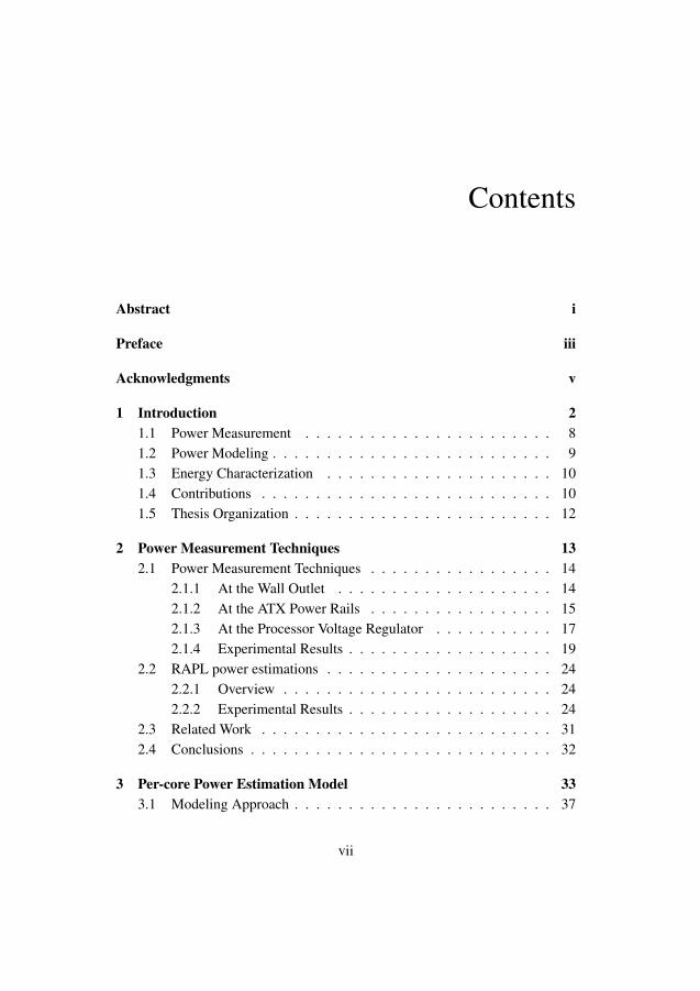
gives 1000 Sa/s. We use a CPU-bound test workload consisting of a 32×32 matrixmultiplication in an infinite loop.
Coarse-grain Power Variance. Fig. 2.5 shows power measurement results acrossthe three different points as we vary the number of active cores. Steps in the powerconsumption are captured by all measurement setups. The low sampling frequency ofthe wall-socket power meter prevents it from capturing short and sharp peaks in power(probably caused by background OS activity). The power consumption changes weobserve at the wall outlet are at least 13 watts from one activity level to another. At suchcoarse-grained power variation, the power readings at wall outlet are strongly correlatedwith power readings at the ATX power rails and CPU voltage regulator.
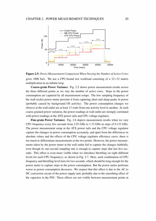
Fine-grain Power Variance. Fig. 2.6 depicts measurement results when we varyCPU frequency every five seconds from 2.93 GHz to 1.33 GHz in steps of 0.133 GHz.The power measurement setup at the ATX power rails and the CPU voltage regulatorcapture the changes in power consumption accurately, and apart from the differences inabsolute values and the effects of the CPU voltage regulator efficiency curve, there isnot much to differentiate measurements at the two points. However, the power measure-ments taken by the power meter at the wall outlet fail to capture the changes faithfully,even though its one-second sampling rate is enough to capture steps that last five sec-onds. This effect is even more visible when we introduce throttling (at eight differentlevels for each CPU frequency), as shown in Fig. 2.7. Here, each combination of CPUfrequency and throttling level lasts for two seconds, which should be long enough for thepower meter to capture steps in the power consumption. But the power meter performsworse as power consumption decreases. We suspect that this effect is due to the AC toDC conversion circuit of the power supply unit, probably due to the smoothing effect ofthe capacitor in the PSU. These effects are not visible between measurement points at
CHAPTER 2. POWER MEASUREMENT TECHNIQUES 21
0 20000 40000 60000 80000 100000Time (msec)
0
50
100
Pow
er (W
)Outlet PowerMB CPU PowerATX CPU Power
CPU Idle
2.93GHz 2.80
GHz2.67GHz 2.53
GHz 2.40GHz
2.27GHz
2.13GHz 2.00
GHz1.87GHz
1.73GHz
1.60GHz
1.47GHz
1.33GHz
Figure 2.6: Power Measurement Comparison When Varying Core Frequency
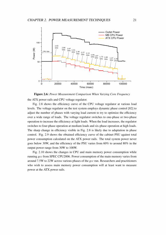
the ATX power rails and CPU voltage regulator.Fig. 2.8 shows the efficiency curve of the CPU voltage regulator at various load
levels. The voltage regulator on the test system employs dynamic phase control [82] toadjust the number of phases with varying load current to try to optimize the efficiencyover a wide range of loads. The voltage regulator switches to one-phase or two-phaseoperation to increase the efficiency at light loads. When the load increases, the regulatorswitches to four-phase operation at medium loads and six-phase operation at high loads.The sharp change in efficiency visible in Fig. 2.8 is likely due to adaptation in phasecontrol. Fig. 2.9 shows the obtained efficiency curve of the cabinet PSU against totalpower consumption calculated on the ATX power rails. The total system power nevergoes below 30W, and the efficiency of the PSU varies from 60% to around 80% in theoutput power range from 30W to 100W.
Fig. 2.10 shows the changes in CPU and main memory power consumption whilerunning gcc from SPEC CPU2006. Power consumption of the main memory varies fromaround 7.5W to 22W across various phases of the gcc run. Researchers and practitionerswho wish to assess main memory power consumption will at least want to measurepower at the ATX power rails.

CHAPTER 2. POWER MEASUREMENT TECHNIQUES 22
0 200000 400000 600000Time (msec)
0
50
100
Pow
er(W
)
Outlet PowerMB CPU PowerATX CPU Power
CPU Idle
2.93GHz 2.80
GHz 2.67GHz 2.53
GHz 2.40GHz
2.27GHz
2.13GHz 2.00
GHz 1.87GHz 1.73
GHz1.60GHz
1.47GHz
1.33GHz
1.20GHz
Figure 2.7: Power Measurement Comparison When Varying Core Frequency Together
with Throttling Level
0 10 20 30 40 50
MB CPU Power (W)
0
20
40
60
80
100
E
ffic
iency (
%)
Figure 2.8: Efficiency Curve of CPU Voltage Regulator

CHAPTER 2. POWER MEASUREMENT TECHNIQUES 23
0 20 40 60 80 100
ATX Total Power (W)
0
20
40
60
80
100
E
ffic
ien
cy (
%)
Figure 2.9: Efficiency Curve of the PSU
0 20000 40000 60000
Time (msec)
0
50
100
P
ow
er
(W)
MB CPU Power
ATX DIMM Power
ATX CPU Power
Figure 2.10: Power Measurement Comparison for the CPU and DIMM (Running gcc)

CHAPTER 2. POWER MEASUREMENT TECHNIQUES 24
2.2 RAPL power estimations
2.2.1 OverviewIntel introduced Running Average Power Limit (RAPL) interface on the Sandy Bridgemicroarchitecture. The programmers can use the RAPL interface for enforcing powerconsumption constraint on the processor. This interface includes non-architectural Model-specific registers (MSRs) for setting the power limit and reading the energy consumptionstatus of the processor power domains like processor die and DRAM2. The energy ex-penditure information provided by the initial implementations of RAPL interface was notbased on actual current measurement from physical sensors, but a power model based onperformance events and probably other inputs like temperature and supply voltage [44].The later RAPL implementations, especially in server grade desktops use actual mea-surement to report energy expenditure [83]. However, this distinction between model-ing and measurement for RAPL is not publicly available for each individual processormodel. In this section, we test the accuracy of RAPL values without assuming one wayor another. In the following sections, we compare power measurement readings fromRAPL and the ATX power rails.
2.2.2 Experimental ResultsWe use Intel CoreTMi7 4770 processor to compare power measurement results at theATX power rails and Intel’s RAPL energy counter. For reading the RAPL energycounter, we use the x86-MSR driver to read the RAPL energy counter MSR calledMSR_PKG_ENERGY_STATUS. We set up a real-time timer that raises SIGALRM atconfigured intervals to read the MSR. We divide the RAPL energy values by the sam-pling interval in seconds to report average power consumption over the sampling in-terval. The ATX power measurement infrastructure is the same as described for IntelCoreTMi7 870 processor. Below we describe our experiments to validate the RAPL en-ergy counter readings.
RAPL Overhead. One of the major differences between measuring power usingRAPL and other techniques shown in Figure 2.1 is that the RAPL measurements aredone on the same machine that is being tested. As a result, reading the RAPL energycounter at frequent intervals adds some overhead to the system power. To test this,we run our RAPL counter reading tool at the sampling frequency of 1 Sa/s, 10 Sa/sand 1000 Sa/s and monitor the change in system power consumption on the ATX CPUpower rails. The results from this experiment are shown in Fig. 2.11. The spikes in
2The DRAM energy status counter is only available on server platforms.

CHAPTER 2. POWER MEASUREMENT TECHNIQUES 25
0 10000 20000 30000
Time (msec)
0
5
10
15
Pow
er
(W)
1000 S/s10 S/s1 S/s
Figure 2.11: Power Overhead Incurred While Reading the RAPL Energy Counter
power consumption visible in the figure indicate the starting of the RAPL reading utility.These spikes mainly result from loading dynamic libraries and can be ignored, assum-ing that the RAPL utility is started before running any benchmark under test. Thesespikes however act as useful synchronization points to overlap readings from RAPL andthe ATX power rails. For calculating the RAPL power overhead, we concentrate on theCPU power consumption after the initial power spike. As seen from the figure, readingthe RAPL MSR every second and every 100ms adds no discernible power consump-tion to the idle system power, but reading the RAPL counter every 1ms adds 0.1W ofpower overhead. However, this small power overhead comes mainly from generatingSIGALRM every millisecond and not from reading the MSR. Hence, if the reading ofRAPL energy counter is done as part of the existing software infrastructure like a kernelscheduler, this will not add discernible overhead to CPU power consumption.
RAPL Resolution. As per the Intel specification manual [84], the RAPL energycounter is updated at the interval of approximately 1ms. To test this update frequency,we run the matrix multiplication application described in Section 2.1.4 while readingthe RAPL energy status counter every 1ms. We sample the ATX power rails every10µS and average over 100 samples. The results from this experiment are shown inFig. 2.12. Although the RAPL readings follow the same curve as those from the ATXpower rails, two things are of note here. First, the RAPL readings show more deviationfrom the mean than the ATX readings. Second, there are huge deviations from the meanat periodic intervals of around 1.6-1.7 seconds. Hähnel et al. [74] observe that the RAPLcounter is not updated exactly at 1ms. As per their experiments, there can be a deviationof a few tens of thousands of cycles in the periodic interval at which the RAPL counteris updated on a given platform. This explains the small deviations from the mean we

CHAPTER 2. POWER MEASUREMENT TECHNIQUES 26
2 4 6 8 10 12 14 16 18 20
Time (sec)
0
20
40
60
80
P
ow
er
(W)
RAPL Power
ATX CPU Power
Figure 2.12: Power Measurement Comparison for the ATX and RAPL at the RAPL
Sampling Rate of 1000 Sa/s
see in our RAPL readings. They also observe that when the CPU switches to SystemManagement Mode (SMM), the RAPL update is delayed until after the CPU comesout of SMM mode. This results in the RAPL energy counter showing no incrementbetween two successive readings, creating a negative deviation. The next update to thecounter increments the energy value expended by the processor in last 2ms instead of1ms, creating a positive deviation. On our system, the CPU switches to SMM every1.6-1.7 seconds, which causes inaccurate energy readings.
RAPL Sensitivity. We test the sensitivity of the RAPL readings to coarse-grainedand fine-grained changes in CPU power consumption. We first repeat the DVFS testfrom Fig. 2.6 in Section 2.1.4 and take the power measurement readings from the ATXpower rail and RAPL. Each DVFS operating point is maintained for five seconds. TheATX power is sampled at 10000 Sa/s while the RAPL counter is sampled at 10 Sa/s. Theresults from this test are shown in Fig. 2.13. The RAPL measurement curve follows theATX measurement curve faithfully, although their y-axis scales are necessarily different.This test verifies the RAPL sensitivity to coarse-grain changes in power consumption.
To test the sensitivity of RAPL to fine-grain changes, we use a microbenchmarkwhich writes to a buffer in a loop, and every 20 seconds, the buffer size is increasedto increase the cache miss rate. This results in gradual increase in power consumptionevery 20 seconds. We run this microbenchmark at two fixed frequencies: 3.4 GHz and800 MHz and compare the power consumption values from ATX CPU rail and RAPL.The results are shown in Figure 2.14 and Figure 2.15 for 3.4 GHz and 800 MHz respec-tively. At 3.4 GHz, the step increment in cache miss rate results in power consumptionincrement of 1W–1.2W as measured at ATX CPU power rail. As the results show, RAPLsensitivity is high enough to track power consumption changes in that range. But when

CHAPTER 2. POWER MEASUREMENT TECHNIQUES 27
20 40 60 80 100
Time (sec)
0
10
20
30
40
50
P
ow
er
(W)
RAPL Power
ATX CPU Power
Figure 2.13: Coarse-grain Sensitivity Test for ATX and RAPL: Frequency Change Test
50 100 150 200 250
Time (sec)
0
10
20
30
40
50
P
ow
er
(W)
RAPL Power
ATX CPU Power
Figure 2.14: Fine-grain Sensitivity Test for ATX and RAPL at 3.4 GHz
we run the same experiment at 800 MHz, the power consumption increment is only0.1W–0.2W. The total power consumption increment at ATX rail from the start to theend of the experiment is 0.99W, which is not detected by RAPL. This highlights thelimitation of RAPL when detecting change in power consumption of smaller than 1W.
Next we test the sensitivity of RAPL power measurement to change in package tem-perature. The static power consumption of the CMOS circuit is dependent on supplyvoltage and temperature. If the voltage and the core activity is fixed, the change inpackage temperature should be directly correlated with the change in power consump-tion. To conduct this experiment, we fix the core and uncore voltage and frequency fromBIOS and put all the cores in active C-state (C0: power management state where theCPU is fully turned on). We then use a hot air gun to increase package temperature

CHAPTER 2. POWER MEASUREMENT TECHNIQUES 28
50 100 150 200 250
Time (sec)
0
2
4
6
8
10
P
ow
er
(W) RAPL Power
ATX CPU Power
Figure 2.15: Fine-grain Sensitivity Test for ATX and RAPL at 800 MHz
0 50 100 150 200 250 300 350 400
Time (s)
0
5
10
15
20
Po
we
r (W
)
ATX
RAPL
0
20
40
60
80
Te
mp
era
ture
(C)
Temp
Figure 2.16: Power Measurement Comparison for ATX and RAPL with Varying Tem-
perature
and sample the power measurement values at ATX and RAPL every second. The re-sults from this experiment are depicted in Figure 2.16. As we can see from the results,because of lower sensitivity of RAPL, the correlation between power measurement atATX and temperature is much stronger than the correlation between RAPL and tem-perature values. Statistically, the correlation coefficient ρ between ATX power valuesand temperature was measured to be 0.9857 while that between RAPL and temperaturewas 0.9127. These results highlight the limitation of RAPL in accurately detecting thechange in power consumption due to temperature change.
Next, we test the ability of RAPL to detect changes power consumption at variouslevels of temporal granularity. We simulate a real-time application in which a task isstarted at fixed periodic intervals. We compare power measurement from RAPL andATX while varying the task period. We set up a timer to raise SIGALRM signal, and a

CHAPTER 2. POWER MEASUREMENT TECHNIQUES 29
matrix multiplication task is started at every timer interrupt. The matrix multiplicationloop is configured to occupy about 66% of the time period. We run this experimentfor three different periods: 100ms, 10ms, and 1ms. We gather samples between twoconsecutive SMM switches. We read the RAPL counter every 1ms. We sample the ATXpower rails every 5µS and average over 20 samples. The results from this experiment areshown in Fig. 2.17. For the 100ms and 10ms period, the RAPL readings closely followthe ATX readings, although they are off by 1ms when the power consumption changessuddenly. As expected, for the 1ms period test, RAPL is unable to capture the powerconsumption curve but accurately estimates the average power consumption.
RAPL Accuracy: We perform an experiment to test the ability of RAPL to reportaccurate power measurement values while running a test benchmark that consists of in-teger operations, floating-point operations and memory operations in different phases.For this experiment, we sample the RAPL energy counter at 100Sa/S. We sample theATX CPU power rails at 10000 Sa/s and then average over 100 samples. We also sam-ple the ATX 5V power rails, which on our system mainly supplies the DRAM memory.We run this experiment at 3.4 GHz. The results are shown in Fig. 2.18. The deviationsthat we see in Fig. 2.12 due to CPU switching to SMM are visible in this Fig. 2.18 aswell. Because we sample the RAPL counter every 10ms instead of 1ms, we only see10% deviation from the mean instead of 100%. Apart from these deviations that occurevery 1.7 second (effectively one out of 170 samples), the RAPL energy readings areaccurate across the integer, floating-point and memory-intensive phases. To quantifythe RAPL power estimation accuracy, we calculate Spearman’s rank correlation coeffi-cient for RAPL and ATX CPU readings for the microbenchmark run. The correlationcoefficient is ρ=0.9858.
Sample values from the ATX show that DRAM power is significant, which is notcaptured by the RAPL package energy counter. Power-aware computing methodolo-gies must take this into consideration. The RAPL interfaces on Intel processors forserver platforms include an energy counter for the DRAM domain called MSR_DRAM_ENERGY_STATUS. This can be useful for assessing the power consumption of theDRAM memory.
Based upon our experimental results, we conclude that the RAPL energy counter isgood for estimating energy over a duration of more than few milliseconds. However,when the researcher is interested in instantaneous power trends, especially peak powertrends, sampling the actual power consumption using an accurate measurement infras-tructure (like ours) is a better choice.

CHAPTER 2. POWER MEASUREMENT TECHNIQUES 30
100 200 300 400
Time (msec)
0
5
10
15
20
P
ow
er
(W)
RAPL Power
ATX CPU Power
(a) 100ms period test
10 20 30 40
Time (msec)
0
5
10
15
20
P
ow
er
(W)
RAPL Power
ATX CPU Power
(b) 10ms period test
1 2 3 4
Time (msec)
0
5
10
15
20
P
ow
er
(W)
RAPL Power
ATX CPU Power
(c) 1ms period test
Figure 2.17: Power Measurement Comparison for ATX and RAPL with Varying Real-
time Application Period

CHAPTER 2. POWER MEASUREMENT TECHNIQUES 31
200 400 600 800
Time (sec)
0
20
40
60
P
ow
er
(W)
RAPL Power
ATX CPU Power
ATX DIMM Power
Figure 2.18: RAPL Accuracy Test for Test Benchmark
2.3 Related WorkHackenberg et al. [85] compare several measurement techniques for signal quality, ac-curacy, timing resolution, and overhead. They use both Intel and AMD systems in theirstudy. Their experimental results complement our results. There have been many inter-esting studies on power-modeling and power-aware resource management. These em-ploy various means to measure empirical power. Rajamani et al. [34] use on-board senseresistors located between the processor and voltage regulators to measure power con-sumed by the processor. They use a National Instruments isolation amplifier and data ac-quisition unit to filter, amplify, and digitize their measurements. Isci and Martonosi [33]measure current on the 12V ATX power lines using clamp ammeters, that are hooked to adigital multimeter (DMM) for data collection. The DMM is connected to a data loggingmachine via an RS232 serial port. Contreras and Martonosi [51] use jumpers on theirIntel XScaleTM development board to measure the power consumption of the CPU andmemory separately. They feed the measurements to a LeCroy oscilloscope for sampling.Cui et al. [35] also measure the power consumption at the ATX power rails. They usecurrent-sense resistors and amplifiers to generate sense voltages (instead of using cur-rent transducers), and they log their measurements using a digital multimeter. Bedard etal. [77] build their own hardware that combines the voltage and current measurementsand host interface into one solution. They use an Analog Devices ADM1191 digitalpower monitor to sense voltage and current values and an Atmel R© microcontroller tosend the measured values to a host USB port. Hähnel et al. [74] experiment with the up-date granularity of the RAPL interface and report practical considerations for using theRAPL energy counter for power measurement. We find their results useful in explainingour experiments. Ge et al. [86] propose a framework to provide in-depth analysis of

CHAPTER 2. POWER MEASUREMENT TECHNIQUES 32
energy expenditure of individual components of the system like fans, disks, processors,DRAM, and motherboard. Their framework uses a combination of hardware resources(sensors, power meter, data acquisition unit) and software (drivers, instrumentation APIsand analysis tools).
2.4 ConclusionsIn this chapter, we demonstrate different techniques that can be employed to measurepower consumption: using off-the-shelf power meter at wall outlet, using current trans-ducers at ATX power rails and by sampling the current monitor pin of CPU’s onboardvoltage regulator. We compare the different techniques in terms of accuracy, sensitivityand temporal granularity and discuss their advantages and disadvantages. We concludethat power measurement at ATX power rails provide the best balance between accuracyand accessibility. We test Intel’s RAPL energy counter results for overhead, accuracy,and update granularity. We compare ATX power measurements with values reportedby RAPL. We conclude that the RAPL package energy counter incurs almost no poweroverhead and is fairly accurate for estimating energy over periods of more than few tensof milliseconds. However, because of irregularities in the frequency at which the RAPLcounter is updated, it shows deviations from the average power when it is sampled at afaster rate.

3Per-core Power Estimation Model
Power measurement techniques described in Chapter 2 are essential for analyzing thepower consumption of systems under test. However, these measurement techniques donot provide detailed information on the power consumption of individual processor coresor microarchitectural units (e.g., caches, floating point units, integer execution units). Todevelop resource-management mechanisms for an individual processor, system design-ers need to analyze power consumption at the granularity of processor cores or eventhe components within a processor core. This information can be provided by placingon-die digital power meters, but that increases the chip’s hardware cost. Hence, sup-port for such fine-grained digital power meters is limited by chip manufacturers. Evenwhen measurement facilities exist, their viability for use in OS or user-level power-awaretechniques is limited either because the measured values are exposed to the software orthe power/energy breakdown is not detailed enough. Indeed, power sensing, actuation,and management support is more often implemented at the blade level with a separatecomputer monitoring output [87, 88].
An alternative to hardware support for fine-grained digital power meters is to es-timate the power consumption at the desired granularity using software power models.Such models can identify various power-relevant events in the targeted microarchitecture
33

CHAPTER 3. PER-CORE POWER ESTIMATION MODEL 34
and then track those events to generate a representative power consumption value. Wecan characterize software power estimation models by the following attributes:
• Portability. The model should be easy to port from one platform to another;
• Scalability. The model should be easy to scale across varying number of activecores and across different CPU voltage-frequency points;
• CPU Usage. The model’s CPU footprint should be negligible, so as not to pollutethe power consumption values of the system under test;
• Accuracy. The model’s estimated values should closely follow the empiricallymeasured power of the device that is modeled;
• Granularity. The model should provide power consumption estimates at thegranularity desired for the problem description (per core, per microarchitecturalmodule, etc.); and
• Speed. The model should supply power estimation values to the software at min-imal latency (preferably within microseconds).
In this thesis, we develop a power model that uses performance counters and temper-ature to generate accurate per-core power estimates in real time, with no off-line profilingor tracing. We build upon the power model developed by Singh et al. [52, 68] and in-clude some of their data for comparison. We validate their model on AMD K8 and IntelCoreTMi7 architectures. Below we explain our choice of using performance counters andtemperature to develop the model.
Performance Counters. We use performance counters for model formation be-cause the power models need a mechanism to track CPU activities with low overhead.Most modern processors are equipped with a Performance Monitoring Unit (PMU) pro-viding the ability to count the microarchitectural events of the processor. PMCs areavailable individually for each core and hence can be used to create core-specific mod-els. This allows programmers to analyze core performance, including the interactionbetween programs and the microarchitecture, in real time on real hardware, rather thanrelying on simplified and less accurate performance results from simulations. The PMUsprovide a wide variety of performance events. These events can be counted by mappingthem to a limited set of Performance Monitoring Counter (PMC) registers. For exam-ple, on Intel and AMD platforms, these performance counter registers are accessible asModel Specific Registers (MSRs). Also called Machine Specific Registers, these arenot necessarily compatible across processor families. Software can configure the perfor-mance counters to select which events to count. The PMCs can be used to count eventslike cache misses, micro-operations retired, stalls at various stages of an out-of-orderpipeline, floating point/memory/branch operations executed, and many more. Although,
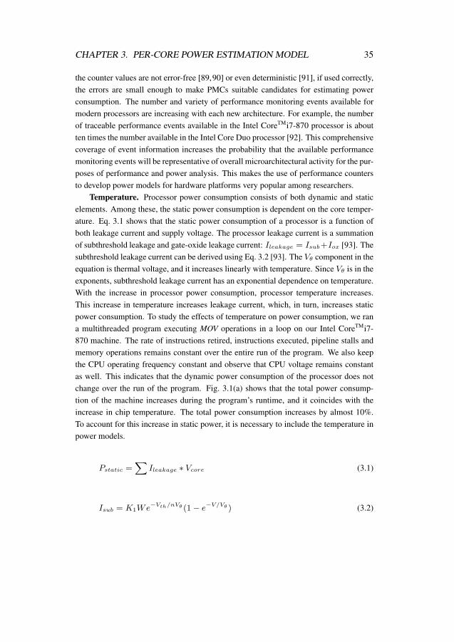
CHAPTER 3. PER-CORE POWER ESTIMATION MODEL 35
the counter values are not error-free [89,90] or even deterministic [91], if used correctly,the errors are small enough to make PMCs suitable candidates for estimating powerconsumption. The number and variety of performance monitoring events available formodern processors are increasing with each new architecture. For example, the numberof traceable performance events available in the Intel CoreTMi7-870 processor is aboutten times the number available in the Intel Core Duo processor [92]. This comprehensivecoverage of event information increases the probability that the available performancemonitoring events will be representative of overall microarchitectural activity for the pur-poses of performance and power analysis. This makes the use of performance countersto develop power models for hardware platforms very popular among researchers.
Temperature. Processor power consumption consists of both dynamic and staticelements. Among these, the static power consumption is dependent on the core temper-ature. Eq. 3.1 shows that the static power consumption of a processor is a function ofboth leakage current and supply voltage. The processor leakage current is a summationof subthreshold leakage and gate-oxide leakage current: Ileakage = Isub+Iox [93]. Thesubthreshold leakage current can be derived using Eq. 3.2 [93]. The Vθ component in theequation is thermal voltage, and it increases linearly with temperature. Since Vθ is in theexponents, subthreshold leakage current has an exponential dependence on temperature.With the increase in processor power consumption, processor temperature increases.This increase in temperature increases leakage current, which, in turn, increases staticpower consumption. To study the effects of temperature on power consumption, we rana multithreaded program executing MOV operations in a loop on our Intel CoreTMi7-870 machine. The rate of instructions retired, instructions executed, pipeline stalls andmemory operations remains constant over the entire run of the program. We also keepthe CPU operating frequency constant and observe that CPU voltage remains constantas well. This indicates that the dynamic power consumption of the processor does notchange over the run of the program. Fig. 3.1(a) shows that the total power consump-tion of the machine increases during the program’s runtime, and it coincides with theincrease in chip temperature. The total power consumption increases by almost 10%.To account for this increase in static power, it is necessary to include the temperature inpower models.
Pstatic =∑
Ileakage ∗ Vcore (3.1)
Isub = K1We−Vth/nVθ (1− e−V/Vθ ) (3.2)
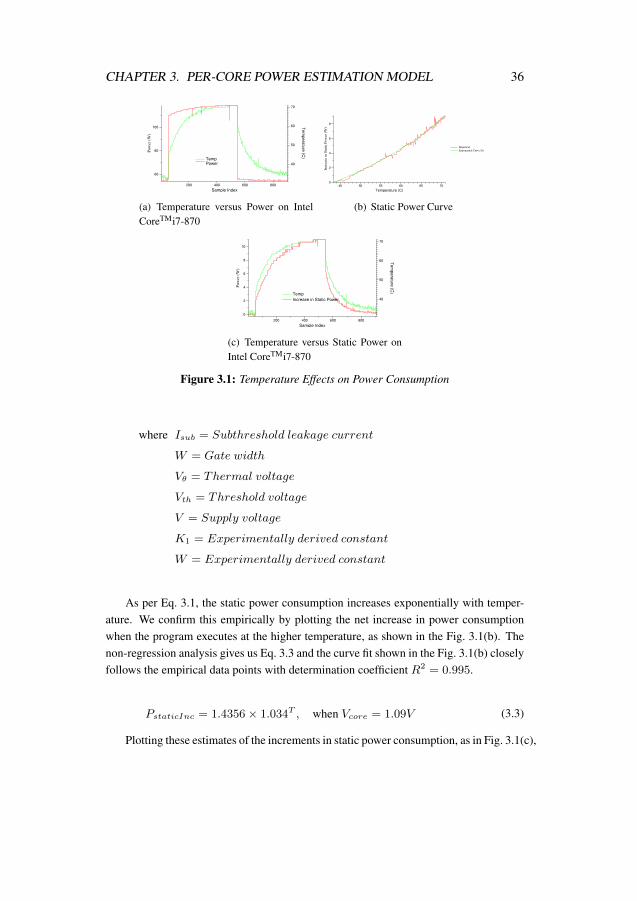
CHAPTER 3. PER-CORE POWER ESTIMATION MODEL 36
200 400 600 800
Sample Index
60
80
100
Pow
er
(W)
Power 40
50
60
70
Tem
pera
ture
(C)
Temp
(a) Temperature versus Power on IntelCoreTMi7-870
45 50 55 60 65 70
Temperature (C)
0
2
4
6
8
Incr
ease
in
Sta
tic
Po
wer
(W
)
Empirical
Exponential Curve Fit
(b) Static Power Curve
200 400 600 800
Sample Index
0
2
4
6
8
10
Pow
er
(W)
Increase in Static Power 40
50
60
70T
em
pera
ture
(C)
Temp
(c) Temperature versus Static Power onIntel CoreTMi7-870
Figure 3.1: Temperature Effects on Power Consumption
where Isub = Subthreshold leakage current
W = Gate width
Vθ = Thermal voltage
Vth = Threshold voltage
V = Supply voltage
K1 = Experimentally derived constant
W = Experimentally derived constant
As per Eq. 3.1, the static power consumption increases exponentially with temper-ature. We confirm this empirically by plotting the net increase in power consumptionwhen the program executes at the higher temperature, as shown in the Fig. 3.1(b). Thenon-regression analysis gives us Eq. 3.3 and the curve fit shown in the Fig. 3.1(b) closelyfollows the empirical data points with determination coefficient R2 = 0.995.
PstaticInc = 1.4356× 1.034T , when Vcore = 1.09V (3.3)
Plotting these estimates of the increments in static power consumption, as in Fig. 3.1(c),

CHAPTER 3. PER-CORE POWER ESTIMATION MODEL 37
explains the gradual rise in total power consumption when the dynamic behavior of aprogram remains constant. Instead of using a non-linear function, we approximate thestatic power increase as a linear function of temperature. This is a fair approximationconsidering that the non-linear equation given in Eq. 3.3 can be closely approximatedwith the linear equation given in Eq. 3.4 with determination coefficient R2 = 0.989 (forthe range in which die temperature changes occur). This linear approximation avoids theadded cost of introducing an exponential term in the power model computation.
PstaticInc = 0.359× T − 16.566, when Vcore = 1.09V (3.4)
Modern processors allow programmers to read temperature information for eachcore from on-die thermal diodes. For example, Intel platforms report relative core tem-peratures on-die via Digital Thermal Sensors (DTS), which can be read by softwarethrough the MSRs or the Platform Environment Control Interface (PECI) [94]. Thisdata is used by the system to regulate CPU fan speed or to throttle the processor in caseof overheating. Third party tools like RealTemp and CoreTemp on Windows and open-source software like lm-sensors on Linux can be used to read data from the thermal sen-sors. As Intel documents indicate [94], the accuracy of temperature readings providedby the thermal sensors varies, and the values reported may not always match the actualcore temperatures. Because of factory variation and individual DTS calibration, readingaccuracy varies from chip to chip. The DTS equipment also suffers from slope errors,which means that temperature readings are more accurate near the T-junction max (themaximum temperature that cores can reach before thermal throttling is activated) thanat lower temperatures. DTS circuits are designed to be read over reasonable operatingtemperature ranges, and the readings may not show lower values than 20◦C even if theactual core temperature is lower. Since DTS is primarily created as a thermal protectionmechanism, reasonable accuracy at high temperatures is acceptable. This affects the ac-curacy of power models that use core temperature. Researchers and practitioners shouldread the processor model datasheet, design guidelines, and errata to understand the lim-itations of their respective thermal monitoring circuits, and they should take correctivemeasures when deriving their power models, if required.
3.1 Modeling ApproachOur approach to power modeling is workload-independent and does not require appli-cation modification. To show the effectiveness of our models, we perform two types ofstudies:
• We demonstrate accuracy and portability on five CMP platforms;
CHAPTER 3. PER-CORE POWER ESTIMATION MODEL 38
• We use the model in a power-aware scheduler to maintain a power budget
Studying sources of model error highlights the need for better hardware support forpower-aware resource management, such as fine-grained power sensors across the chipand more accurate temperature information. Our approach nonetheless shows promisefor balancing performance, power, and thermal requirements for platforms from embed-ded real-time systems to consolidated data centers, and even to supercomputers.
In the rest of the chapter, we first present the details of how we build our model,and then we discuss how we validate them. Our evaluation analyzes the model’s compu-tation overhead(Section 3.3.1) and accuracy(Section 3.3.2). We then explain the meta-scheduler that we use as a proof-of-concept for showing the effectiveness of our modelin Section 3.4.
3.2 Methodology
3.2.1 Counter SelectionSelecting appropriate PMCs to use is extremely important with respect to accuracy ofthe power model. We choose counters that are most highly correlated with measuredpower consumption. The chosen counters must also cover a sufficiently large set ofevents to ensure that they capture general application activity. If the chosen countersdo not meet these criteria, the model will be prone to error. The problem of choosingappropriate counters for power modeling has been handled in different ways by previousresearchers.
Research studies that estimate power for an entire core or a processor [34, 42, 51],use a small number of PMCs. Those that aim to construct decomposed power modelsto estimate the power consumption of sub-units of a core [48–50] tend to monitor morePMCs. The number of counters needed depends on the model granularity and the accept-able level of complexity. Also, most modern processors allow simultaneous counting ofonly a limited number (two/four/eight) microarchitectural events. Hence, using morecounters in the model requires interleaving the counting of events and extrapolating thecounter values over the total sampling period. This reduces the accuracy of absolutecounter values but allows researchers to track more counters.
To choose appropriate performance counters for developing our power-estimationmodel, we divide the available counters into four categories and then choose one counterfrom each category based upon statistical correlation [52,68]. This ensures that the cho-sen counters are comprehensive representations of the entire microarchitecture and arenot biased towards any particular section. Caches and floating point units form a largepart of the chip real estate, and thus PMCs that keep track of their activity factors would
CHAPTER 3. PER-CORE POWER ESTIMATION MODEL 39
be useful additions to the total power consumption information. Depending on the plat-form, multiple counters will be available in both these categories. For example, we cancount the total number of cache references as well as the number of cache misses for var-ious cache levels. For floating point operations, depending upon the processor model,we can count (separately or in combination) the number of multiplication, addition, anddivision operations. Because of the deep pipelining of modern processors, we can alsoexpect out-of-order logic to account for a significant amount of power. Stalls due tobranch mispredictions or an empty instruction decoder may reduce average power con-sumption over a fixed period of time. On the other hand, pipeline stalls caused by fullreservation stations and reorder buffers will be positively correlated with power becausethese indicate that the processor has extracted enough instruction-level parallelism tokeep the execution units busy. Hence, pipeline stalls indicate not just the power usageof out-of-order logic but of the executions units, as well. In addition, we would liketo use a counter that can cover all the microarchitectural components not covered bythe above three categories. This includes, for example, integer execution units, branchprediction units, and Single Instruction Multiple Data (SIMD) units. These events canbe monitored using the specific PMCs tied to them or by a generalized counter like to-tal instructions/micro-operations (UOPS) retired/executed/issued/decoded. To constructa power model for individual sub-units, we need to identify the respective PMCs thatrepresent each sub-unit’s utilization factors.
To choose counters via statistical correlation, we run a training application whilesampling the performance counters and collecting empirical power measurement values.Fig. 3.2 shows simplified pseudo-code for the microbenchmark [52] that we use to de-velop our power model. Here, different phases of the microbenchmark exercise differentparts of the microarchitecture. Since the number of relevant PMCs will most likely bemore than the limit on simultaneously monitored counters, multiple training runs arerequired to gather data for all desired counters.
Once the performance counter values and the respective empirical power consump-tion values are collected, we use a statistical correlation to establish the correlation be-tween performance events (counter values normalized to the number of instructions ex-ecuted) and power. This guides our selection of the most suitable events for use in thepower model. Obviously, the type of correlation method used can affect the model ac-curacy. We use Spearman’s rank correlation [95] to measure the relationship betweeneach counter and power. The performance counters and power values can be linear ornon-linear. Using the rank correlation, as opposed to using correlation methods likePearson’s, ensures that this non-linear relationship does not affect the correlation coeffi-cient.
For example, Table 3.1 shows the most power-relevant counters divided categori-

CHAPTER 3. PER-CORE POWER ESTIMATION MODEL 40
for (i=0;i<interval*PHASE_CNT;i++) {
phase = (i/interval) % PHASE_CNT;
switch(phase) {
case 0:
/* do floating point operations */
case 1:
/* do integer arithmetic operations */
case 2:
/* do memory operations with high
locality */
case 3:
/* do memory operations with low locality
*/
case 4:
/* do register file operations */
case 5:
/* do nothing */
.
.
.
}
}
Figure 3.2: Microbenchmark Pseudo-Code
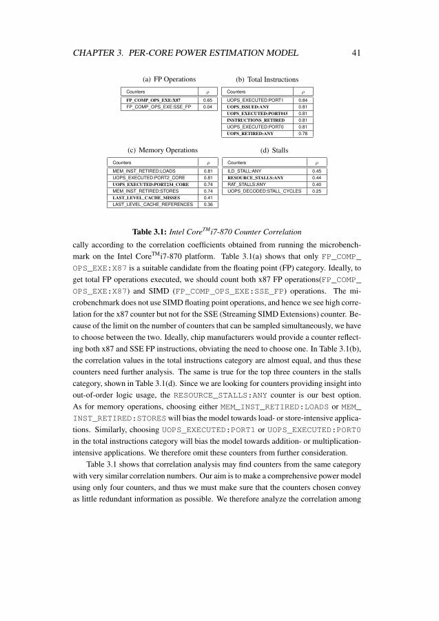
CHAPTER 3. PER-CORE POWER ESTIMATION MODEL 41
(a) FP Operations
Counters ρ
FP_COMP_OPS_EXE:X87 0.65FP_COMP_OPS_EXE:SSE_FP 0.04
(b) Total Instructions
Counters ρ
UOPS_EXECUTED:PORT1 0.84UOPS_ISSUED:ANY 0.81UOPS_EXECUTED:PORT015 0.81INSTRUCTIONS_RETIRED 0.81UOPS_EXECUTED:PORT0 0.81UOPS_RETIRED:ANY 0.78
(c) Memory Operations
Counters ρ
MEM_INST_RETIRED:LOADS 0.81UOPS_EXECUTED:PORT2_CORE 0.81UOPS_EXECUTED:PORT234_CORE 0.74MEM_INST_RETIRED:STORES 0.74LAST_LEVEL_CACHE_MISSES 0.41LAST_LEVEL_CACHE_REFERENCES 0.36
(d) Stalls
Counters ρ
ILD_STALL:ANY 0.45RESOURCE_STALLS:ANY 0.44RAT_STALLS:ANY 0.40UOPS_DECODED:STALL_CYCLES 0.25
Table 3.1: Intel CoreTMi7-870 Counter Correlation
cally according to the correlation coefficients obtained from running the microbench-mark on the Intel CoreTMi7-870 platform. Table 3.1(a) shows that only FP_COMP_
OPS_EXE:X87 is a suitable candidate from the floating point (FP) category. Ideally, toget total FP operations executed, we should count both x87 FP operations(FP_COMP_OPS_EXE:X87) and SIMD (FP_COMP_OPS_EXE:SSE_FP) operations. The mi-crobenchmark does not use SIMD floating point operations, and hence we see high corre-lation for the x87 counter but not for the SSE (Streaming SIMD Extensions) counter. Be-cause of the limit on the number of counters that can be sampled simultaneously, we haveto choose between the two. Ideally, chip manufacturers would provide a counter reflect-ing both x87 and SSE FP instructions, obviating the need to choose one. In Table 3.1(b),the correlation values in the total instructions category are almost equal, and thus thesecounters need further analysis. The same is true for the top three counters in the stallscategory, shown in Table 3.1(d). Since we are looking for counters providing insight intoout-of-order logic usage, the RESOURCE_STALLS:ANY counter is our best option.As for memory operations, choosing either MEM_INST_RETIRED:LOADS or MEM_INST_RETIRED:STORESwill bias the model towards load- or store-intensive applica-tions. Similarly, choosing UOPS_EXECUTED:PORT1 or UOPS_EXECUTED:PORT0in the total instructions category will bias the model towards addition- or multiplication-intensive applications. We therefore omit these counters from further consideration.
Table 3.1 shows that correlation analysis may find counters from the same categorywith very similar correlation numbers. Our aim is to make a comprehensive power modelusing only four counters, and thus we must make sure that the counters chosen conveyas little redundant information as possible. We therefore analyze the correlation among

CHAPTER 3. PER-CORE POWER ESTIMATION MODEL 42
(a) MEM versus INSTR Correlation
UOPS_EXECUTED:PORT234 LAST_LEVEL_CACHE_MISSES
UOPS_ISSUED:ANY 0.97 0.14UOPS_EXECUTED:PORT015 0.88 0.2INSTRUCTIONS_RETIRED 0.91 0.12UOPS_RETIRED:ANY 0.98 0.08
(b) FP versus INSTR Correlation
FP_COMP_OPS_EXE:X87
UOPS_ISSUED:ANY 0.44UOPS_EXECUTED:PORT015 0.41INSTRUCTIONS_RETIRED 0.49UOPS_RETIRED:ANY 0.43
(c) STALL versus INSTR Correlation
RESOURCE_STALLS:ANY
UOPS_ISSUED:ANY 0.25UOPS_EXECUTED:PORT015 0.30INSTRUCTIONS_RETIRED 0.23UOPS_RETIRED:ANY 0.21
Table 3.2: Counter-Counter Correlation
all the counters. To select a counter from the memory operations category, we analyzethe correlation of UOPS_EXECUTED:PORT234_CORE and LAST_LEVEL_CACHE_MISSES with the counters from the total instructions category, as shown in Table 3.2(a).From this table, it is evident that UOPS_EXECUTED:PORT234_CORE is highly cor-related with the instructions counters, and hence LAST_LEVEL_CACHE_MISSES isthe better choice. To choose a counter from the total-instructions category, we analyzethe correlation of these counters with the FP and stalls counters (in Table 3.2(b) andTable 3.2(c), respectively). These correlations do not clearly recommend any particularchoice. In such cases, we can either choose one counter arbitrarily or choose a counterintuitively. UOPS_EXECUTED:PORT015 does not cover memory operations that aresatisfied by cache accesses, instead of main memory. The UOPS_RETIRED:ANY andINSTRUCTIONS_RETIRED counters cover only retired instructions and not those thatare executed but not retired, e.g., due to branch mispredictions. A UOPS_EXECUTED:
ANY counter would be appropriate, but since such a counter does not exist, the next bestoption is UOPS_ISSUED:ANY. This counter covers all instructions issued, so it alsocovers the instructions issued but not executed (and thus not retired).
We use the same methodology to select representative performance counters for allthe machines that we evaluate. Table 3.4 shows the counters we select for the differentplatforms.
3.2.2 Model FormationHaving identified events that contribute significantly to consumed power, we create aformalism to map observed microarchitectural activity and measured temperatures tomeasured power draw. We re-run the microbenchmark sampling just the chosen PMCs,collecting power and temperature data at each sampling interval. We normalize eachtime-sampled PMC value, ei, to the elapsed cycle count to generate an event rate, ri.

CHAPTER 3. PER-CORE POWER ESTIMATION MODEL 43
We then map rise in core temperature, T , and the observed event rates, ri, to core power,Pcore, via a piece-wise model based on multiple linear regression, as in Equation 3.5.We apply non-linear transformations to normalized counter values to account for non-linearity, as in Equation 3.6. The normalization ensures that changing the sampling pe-riod of the readings does not affect the weights of the respective predictors. We developa piecewise power model that achieves better fit by separating the collected samples intotwo bins based on the values of either the memory counter or the FP counter. Breakingthe data using the memory counter value helps in separating memory-bound phases fromCPU-bound phases. Using the FP counter instead of the memory counter to divide thedata helps in separating FP-intensive phases. The selection of a candidate for break-ing the model is machine-specific and depends on what gives a better fit. Regardless,we agree with Singh et. [52, 68] that piecewise linear models better capture processorbehavior.
Pcore =
{F1(g1(r1), · · · , gn(rn), T ), if conditionF2(g1(r1), · · · , gn(rn), T ), else
(3.5)
where ri = ei/(cycle count), T = Tcurrent − Tidle
Fn = p0 + p1 ∗ g1(r1) + ...+ pn ∗ gn(rn) + pn+1 ∗ T (3.6)
As an example, the piecewise linear regression model for the Intel CoreTMi7-870 isshown in Eq. 3.7. Here, rMEM refers to the counter LAST_LEVEL_CACHE_MISSES,rINSTR refers to the counter UOPS_ISSUED, rFP refers to the counter FP_COMP_OPS_EXE:X87, and rSTALL refers to the counter RESOURCE_STALLS:ANY. Thepiecewise model is broken based on the value of the memory counter. For the first partof the piece-wise model, the coefficient for the memory counter is zero (due to the verylow number of memory operations we sampled).
Pcore =
10.9246 + 0 ∗ rMEM + 5.8097 ∗ rINSTR+
0.0529 ∗ rFP + 6.6041 ∗ rSTALL + 0.1580 ∗ T, if rMEM < 1e− 6
19.9097 + 556.6985 ∗ rMEM + 1.5040 ∗ rINSTR+0.1089 ∗ rFP +−2.9897 ∗ rSTALL + 0.2802 ∗ T, if rMEM ≥ 1e− 6
(3.7)

CHAPTER 3. PER-CORE POWER ESTIMATION MODEL 44
3.3 ValidationWe evaluate our models by estimating per-core power for the SPEC 2006 [96], SPEC-OMP [97, 98], and NAS [99] benchmark suites. In our experiments, we run multi-threaded benchmarks with one thread per core, and single-threaded benchmarks withan instance on each core. We use gcc 4.2 to compile our benchmarks for a 64-bit ar-chitecture with optimization flags enabled, and we run all benchmarks to completion.We use the pfmon utility from the perfmon2 library [100] to access the hardware perfor-mance counters. Table 3.3 gives system details of the machines on which we validatedour power model. System power is based on measuring the power supply’s current drawfrom the power outlet when the machine is idle. When we cannot find published val-ues for idle processor power, we sum power draw when powered off and power savedby turning off cdrom and hard disk drives, removing all but one memory DIMM, anddisconnecting fans. We subtract idle core power from idle system power to get uncore(baseline without processor) power. Change in the uncore power itself (due to DRAMor hard drive accesses, for instance) is included in the model estimations. Including tem-perature as a model input accounts for variation in uncore static power. We always runin the active power state (C0).
We use the sensors utility from the lm-sensors library to obtain core temperatures,and we use the Watts Up? Pro power meter [75] described in Chapter 2 to gather powerdata. This meter is accurate to within 0.1W, and it updates once per second. Althoughmeasuring the power at wall outlet has limitations in terms of sensitivity to fine-grainedchanges in power consumption, we use it for our experiments because of its low cost,non-intrusive use, and easy portability. Moreover, we observe that for the benchmarks inour experiments, the power consumption of the system does not change at the granularityof less than one second, and hence sampling power consumption at the rate of 1 sam-ple/second meets our requirement for this modeling approach. Our modeling approachcan easily be adapted to other power measurement techniques, such as those describedin Chapter 2.
We incorporate the power model into a proof-of-concept, power-aware resourcemanager (a user-level meta-scheduler of Singh et al. [52, 68]) designed to maintain aspecified power envelope. The meta-scheduler manages processes non-invasively, re-quiring no modifications to the applications or OS. It does so by suspending/resumingprocesses and, where supported, applying dynamic voltage/frequency scaling (DVFS)to alter core clock rates. For these experiments, we degrade the system power envelopeby 10%, 20%, and 30% for CoreTMi7-870 platform. Lower envelopes render cores in-active, and thus we do not consider them. Finally, we incorporate the model in a kernelscheduler, implementing a pseudo power sensor per core. The device does not exist

CHAPTER 3. PER-CORE POWER ESTIMATION MODEL 45
(a) Configuration Parameters for Intel Platforms
Intel Q6600 Intel Xeon E5430 Intel CoreTMi7-870Cores/Chips 4, dual dual-core 4Frequency (GHz) 2.4 2.0, 2.66 2.93Process (nm) 65 45 45L1 Instruction 32 KB 8-way 32 KB 8-way 32 KB 4-wayL1 Data 32 KB 8-way 32 KB 8-way 32 KB 8-wayL2 Cache 4 MB 16-way shared 6 MB 16-way shared 256 KB 8-way exclusiveL3 Cache N/A N/A 8 MB 16-way sharedMemory Controller off-chip, 2 channel off-chip, 4 channel on-chip, 2 channelMain Memory 4 GB DDR2-800 8 GB DDR2-800 16 GB DDR3-1333Bus (MHz) 1066 1333 1333Max TDP (W) 105 80 95Linux Kernel 2.6.27 2.6.27 2.6.31Idle System Power (W) 141.0 180.0 54.0Idle Processor Power (W) 38.0 27.0 10.0Idle Temperature (◦C) 36 45 30
(b) Configuration Parameters for AMD Platforms
AMD PhenomTM9500 AMD OpteronTM8212Cores/Chips 4 8, quad dual-coreFrequency (GHz) 1.1, 2.2 2.0Process (nm) 65 90L1 Instruction 64 KB 2-way 64 KB 2-wayL1 Data 64 KB 2-way 64 KB 2-wayL2 Cache 512 KB 8-way exclusive 1024 KB 16-way exclusiveL3 Cache 2 MB 32-way shared N/AMemory Controller on-chip, 2 channel on-chip, 2 channelMain Memory 4 GB DDR2-800 16 GB DDR2-667Bus (MHz) 1100, 2200 1000Max TDP (W) 95 95Linux Kernel 2.6.25 2.6.31Idle System Power (W) 84.1 302.6Idle Processor Power (W) 20.1 53.6WIdle Temperature (◦C) 36 33
Table 3.3: Machine Configuration Parameters
(a) PMCs Selected for Intel Platforms
Category Intel Q6600 Intel E5430 Intel CoreTMi7-870
Memory L2_LINES_IN LAST_LEVEL_CACHE_MISSES LAST_LEVEL_CACHE_MISSESInstructions Executed UOPS_RETIRED UOPS_RETIRED UOPS_ISSUEDFloating Point X87_OPS_RETIRED X87_OPS_RETIRED FP_COMP_OPS_EXE:X87Stalls RESOURCE_STALLS RESOURCE_STALLS RESOURCE_STALLS:ANY
(b) PMCs Selected for AMD Platforms
Category AMD PhenomTM9500 AMD OpteronTM8212
Memory L2_CACHE_MISS DATA_CACHE_ACCESSESInstructions Executed RETIRED_UOPS RETIRED_INSTRUCTIONSFloating Point RETIRED_MMX_AND_FP_INSTRUCTIONS DISPATCHED_FPU:OPS_MULTIPLYStalls DISPATCH_STALLS DECODER_EMPTY
Table 3.4: PMCs Selected for Power-Estimation Model

CHAPTER 3. PER-CORE POWER ESTIMATION MODEL 46
Benchmark baseline model (10msec) model (100msec) model (1sec)
ep.A serial 35.68 35.57 36.04 35.59ep.A OMP 4.84 4.89 4.77 4.74ep.A MPI 4.77 4.72 4.73 4.75
cg.A serial 5.82 5.83 5.83 5.83cg.A OMP 1.95 1.95 1.95 1.95cg.A MPI 2.19 2.20 2.20 2.20
ep.B serial 146.53 146.52 145.52 146.77ep.B OMP 19.45 19.33 19.35 19.54ep.B MPI 18.95 19.41 19.12 19.18
cg.B serial 559.58 560.50 560.11 560.10cg.B OMP 91.29 92.64 96.90 89.92cg.B MPI 79.11 79.18 79.18 79.05
Table 3.5: Scheduler Benchmark Times for Sample NAS Applications on the AMD
OpteronTM8212 (sec)
in hardware but is simulated by the power model module. Reads to the pseudo-deviceretrieve the power estimate computed most recently.
3.3.1 Computation OverheadIf computing the model is expensive, its use becomes limited to coarse timeslices. Inthis experiment we study the overhead of our power model to evaluate its use in an OStask scheduler. We use the scheduler developed by Boneti et al. [101] that is specifi-cally tailored to High Performance Computing (HPC) applications that require that theOS introduce little or no overhead. In most cases, this scheduler delivers better per-formance with better predictability, and it reduces OS noise [101, 102]. The model’soverhead depends on 1) the frequency with which the per-core power is updated, and2) the complexity of the operations required to calculate the model. We calculate over-head by measuring execution time for our kernel scheduler running with and withoutreading the PMCs and temperature sensors. We vary the sample period from one minuteto 10 msec. We time applications for five runs and take the average (differences amongruns are within normal execution time variation for real systems). Table 3.5 gives mea-sured times for the scheduler with and without evaluating the model. These data showthat computing the model adds no measurable overhead, even at 10ms timeslices.
3.3.2 Estimation ErrorWe assess model error by comparing our system power estimates to power meter out-put (which our power meter limits to a one-second granularity). We estimate the powerconsumption per core, and then sum up the power consumption for all cores with uncorepower to compare the estimated power consumption with measured values. Figure 3.3through Figure 3.7 1 show percentage median error for the NAS, SPEC-OMP, and SPEC
1Data for Intel Q6600

CHAPTER 3. PER-CORE POWER ESTIMATION MODEL 47
bt cg ep ft lulu-h
pm
g sp ua0
2
4
6
8
10
% M
ed
ian
Err
or
(a) NAS
amm
p
applu
apsi ar
t
fma3
d
mgr
id
quak
e
swim
wup
wise
0
2
4
6
8
10
% M
ed
ian
Err
or
(b) SPEC-OMP
asta
r
bwav
es
bzip2
cactus
ADM
calculix
dealll
gam
ess
gcc
Gem
sFDTD
gobm
k
grom
acs
h264
ref
hmm
erlbm
leslie3d
libqu
antu
mm
cfm
ilc
nam
d
omne
tpp
perlb
ench
povr
ay
sjen
g
soplex
xalanc
bmk
zeus
mp
0
2
4
6
8
10
% M
edia
n E
rror
(c) SPEC 2006
Figure 3.3: Median Estimation Error for the Intel Q6600 system
2006 applications on all systems. Figure 3.8 through Figure 3.12 show standard devia-tion of error for each benchmark suite. The occasional high standard deviations illustratethe main problem with our current infrastructure: instantaneous power measurementsonce per second do not reflect continuous performance counter activity since the lastmeter reading.
Estimation error ranges from 0.3% (leslie3d) to 7.1% (bzip2) for the Intel Q6600system, from 0.3% (ua) to 7.0% (hmmer) for the Intel E5430 system, from 1.02% (bt) to9.3% (xalancbmk) for the AMD PhenomTMsystem, from 1.0% (bt.B ) to 10.7% (soplex) for the AMD OpteronTM8212 system and from 0.17% (art ) to 9.07% (libquantum )for the Intel CoreTMi7-870 system. On Intel Q6600, only five (out of 45) applicationsexhibit median error exceeding 5%; on the Intel E5430, only six exhibit error exceeding5%; on the AMD PhenomTM, eighteen exhibit error exceeding 5%; and on the AMDOpteronTM8212, thirteen exhibit error exceeding 5%. For the Intel CoreTMi7-870, me-dian estimations for only seven applications exceed 5% error. Table 3.6 shows the sum-mary of power estimation errors for our model across all platforms. These data suggessthat our model works better on Intel machines compared to AMD machines.
Figure 3.13 shows model coverage via Cumulative Distribution Function (CDF)plots for the suites. On Q6600, 85% of estimates have less than 5% error, and 98%have less than 10%. On E5430, 73% have less than 5% error, and 99% less than 10%.On PhenomTM, 59% have less than 5% error, and 92% less than 10%. On 8212, 37%

CHAPTER 3. PER-CORE POWER ESTIMATION MODEL 48
bt cg ep ft lulu-h
pm
g sp ua0
2
4
6
8
10
% M
ed
ian
Err
or
(a) NAS
amm
p
applu
apsi ar
t
fma3
d
mgr
id
quak
e
swim
wup
wise
0
2
4
6
8
10
% M
ed
ian
Err
or
(b) SPEC-OMP
asta
r
bwav
es
bzip2
cactus
ADM
calculix
dealll
gam
ess
gcc
Gem
sFDTD
gobm
k
grom
acs
h264
ref
hmm
erlbm
leslie3d
libqu
antu
mm
cfm
ilc
nam
d
omne
tpp
perlb
ench
povr
ay
sjen
g
soplex
xalanc
bmk
zeus
mp
0
2
4
6
8
10
% M
edia
n E
rror
(c) SPEC 2006
Figure 3.4: Median Estimation Error for Intel E5430 system
bt cg ep ft lulu-h
pm
g sp ua0
2
4
6
8
10
% M
ed
ian
Err
or
(a) NAS
amm
p
applu
apsi ar
t
fma3
d
gafo
rt
mgr
id
quak
e
swim
wup
wise
0
2
4
6
8
10
% M
ed
ian
Err
or
(b) SPEC-OMP
asta
r
bwav
es
bzip2
cactus
ADM
calculix
dealll
gam
ess
gcc
Gem
sFDTD
gobm
k
grom
acs
h264
ref
hmm
erlbm
leslie3d
libqu
antu
mm
cfm
ilc
nam
d
omne
tpp
perlb
ench
povr
ay
sjen
g
soplex
xalanc
bmk
zeus
mp
0
2
4
6
8
10
% M
edia
n E
rror
(c) SPEC 2006
Figure 3.5: Median Estimation Error for the AMD PhenomTM9500

CHAPTER 3. PER-CORE POWER ESTIMATION MODEL 49
bt cg ep ft lulu-h
pm
g sp ua0
2
4
6
8
10
% M
ed
ian
Err
or
(a) NAS
amm
p
applu
apsi ar
t
fma3
d
gafo
rt
mgr
id
quak
e
swim
wup
wise
0
2
4
6
8
10
% M
ed
ian
Err
or
(b) SPEC-OMP
asta
r
bwav
es
bzip2
cactus
ADM
calculix
dealll
gam
ess
gcc
Gem
sFDTD
gobm
k
grom
acs
h264
ref
hmm
erlbm
leslie3d
libqu
antu
mm
cfm
ilc
nam
d
omne
tpp
perlb
ench
povr
ay
sjen
g
soplex
xalanc
bmk
zeus
mp
0
2
4
6
8
10
% M
edia
n E
rror
(c) SPEC 2006
Figure 3.6: Median Estimation Error for the AMD OpteronTM8212
bt cg ep ft lulu-h
pm
g sp ua0
2
4
6
8
10
% M
ed
ian
Err
or
(a) NAS
amm
p
applu
apsi ar
t
fma3
d
mgr
id
quak
e
swim
wup
wise
0
2
4
6
8
10
% M
ed
ian
Err
or
(b) SPEC-OMP
asta
r
bwav
es
bzip2
cactus
ADM
calculix
dealll
gam
ess
gcc
Gem
sFDTD
gobm
k
grom
acs
h264
ref
hmm
erlbm
leslie3d
libqu
antu
mm
cfm
ilc
nam
d
omne
tpp
perlb
ench
povr
ay
sjen
g
soplex
xalanc
bmk
zeus
mp
0
2
4
6
8
10
% M
ed
ian
Err
or
(c) SPEC 2006
Figure 3.7: Median Estimation Error for the Intel CoreTMi7

CHAPTER 3. PER-CORE POWER ESTIMATION MODEL 50
bt cg ep ft lulu-h
pm
g sp ua0
2
4
6
8
10
% S
D
(a) NAS
amm
p
applu
apsi ar
t
fma3
d
gafo
rt
mgr
id
quak
e
swim
wup
wise
0
2
4
6
8
10
% S
D
(b) SPEC-OMP
asta
r
bwav
es
bzip2
cactus
ADM
calculix
dealll
gam
ess
gcc
Gem
sFDTD
gobm
k
grom
acs
h264
ref
hmm
erlbm
leslie3d
libqu
antu
mm
cfm
ilc
nam
d
omne
tpp
perlb
ench
povr
ay
sjen
g
soplex
xalanc
bmk
zeus
mp
0
2
4
6
8
10
% S
D
(c) SPEC 2006
Figure 3.8: Standard Deviation of Error for the Intel Q6600 system
bt cg ep ft lulu-h
pm
g sp ua0
2
4
6
8
10
% S
D
(a) NAS
amm
p
applu
apsi ar
t
fma3
d
gafo
rt
mgr
id
quak
e
swim
wup
wise
0
2
4
6
8
10
% S
D
(b) SPEC-OMP
asta
r
bwav
es
bzip2
cactus
ADM
calculix
dealll
gam
ess
gcc
Gem
sFDTD
gobm
k
grom
acs
h264
ref
hmm
erlbm
leslie3d
libqu
antu
mm
cfm
ilc
nam
d
omne
tpp
perlb
ench
povr
ay
sjen
g
soplex
xalanc
bmk
zeus
mp
0
2
4
6
8
10
% S
D
(c) SPEC 2006
Figure 3.9: Standard Deviation of Error for Intel E5430 system

CHAPTER 3. PER-CORE POWER ESTIMATION MODEL 51
bt cg ep ft lulu-h
pm
g sp ua0
2
4
6
8
10
% S
D11
.719
.315
.6
(a) NAS
amm
p
applu
apsi ar
t
fma3
d
gafo
rt
mgr
id
quak
e
swim
wup
wise
0
2
4
6
8
10
% S
D
(b) SPEC-OMP
asta
r
bwav
es
bzip2
cactus
ADM
calculix
dealll
gam
ess
gcc
Gem
sFDTD
gobm
k
grom
acs
h264
ref
hmm
erlbm
leslie3d
libqu
antu
mm
cfm
ilc
nam
d
omne
tpp
perlb
ench
povr
ay
sjen
g
soplex
xalanc
bmk
zeus
mp
0
2
4
6
8
10
% S
D
14.9
12.2
(c) SPEC 2006
Figure 3.10: Standard Deviation of Error for the AMD PhenomTM9500
bt cg ep ft lulu-h
pm
g sp ua0
2
4
6
8
10
% S
D
(a) NAS
amm
p
applu
apsi ar
t
fma3
d
gafo
rt
mgr
id
quak
e
swim
wup
wise
0
2
4
6
8
10
% S
D
(b) SPEC-OMP
asta
r
bwav
es
bzip2
cactus
ADM
calculix
dealll
gam
ess
gcc
Gem
sFDTD
gobm
k
grom
acs
h264
ref
hmm
erlbm
leslie3d
libqu
antu
mm
cfm
ilc
nam
d
omne
tpp
perlb
ench
povr
ay
sjen
g
soplex
xalanc
bmk
zeus
mp
0
2
4
6
8
10
% S
D
(c) SPEC 2006
Figure 3.11: Standard Deviation of Error for the AMD OpteronTM8212

CHAPTER 3. PER-CORE POWER ESTIMATION MODEL 52
bt cg ep ft lulu-h
pm
g sp ua0
2
4
6
8
10
% S
D
(a) NAS
amm
p
applu
apsi ar
t
fma3
d
gafo
rt
mgr
id
quak
e
swim
wup
wise
0
2
4
6
8
10
% S
D
(b) SPEC-OMP
asta
r
bwav
es
bzip2
cactus
ADM
calculix
dealll
gam
ess
gcc
Gem
sFDTD
gobm
k
grom
acs
h264
ref
hmm
erlbm
leslie3d
libqu
antu
mm
cfm
ilc
nam
d
omne
tpp
perlb
ench
povr
ay
sjen
g
soplex
xalanc
bmk
zeus
mp
0
2
4
6
8
10
% S
D
(c) SPEC 2006
Figure 3.12: Standard Deviation of Error for the IntelCoreTMi7
Benchmark Intel Q660 Intel E5430 Intel CoreTMi7-870 AMD PhenomTM AMD 8212
SPEC 2006 1.1 2.8 2.22 3.5 4.80NAS 1.6 3.9 3.11 4.5 2.55SPEC OMP 1.6 3.5 2.02 5.2 3.35Overall 1.2 3.6 2.07 3.8 4.38
Table 3.6: Estimation Error Summary

CHAPTER 3. PER-CORE POWER ESTIMATION MODEL 53
have less than 5% error, and 76% have less than 10%. For the CoreTMi7-870, 82% ofestimates have less than 5% error and 96% have less than 10% error. The vast majorityof estimates exhibit very small error.
These errors are not excessive, but lower is better. Prediction errors are not clus-tered, but are spread throughout application execution. Model accuracy depends on theparticular PMCs available on a given platform. If available PMCs do not sufficientlyrepresent the microarchitecture, model accuracy will suffer. For example, the AMDOpteronTM8212 processor supports no single counter giving total floating point oper-ations. Instead, separate PMCs track different types of floating point operations. Wetherefore choose the one most highly correlated with power. Model accuracy wouldlikely improve if a single PMC reflecting all floating point operations were available. Forprocessor models supporting only two Model Specific Registers for reading PMC val-ues, capturing the activity of four counters requires multiplexing the counting of PMC-related events. This means that events are counted for only half a second (or half thetotal sampling period), and are doubled to estimate the value over the entire period. Thisapproximation can introduce inaccuracies when program behavior is changing rapidly.The model estimation accuracy is also affected by accuracy of hardware sensors. Forinstance, the OpteronTM8212 temperature sensor data suffers with low accuracy [103].
Similarly, even though the microbenchmark tries to cover all scenarios of powerconsumption, the resulting regression model will represent a generalized case. This isespecially true for a model that tries to estimate power for a complex microarchitectureusing limited number of counters. For example, floating point operations can consist ofadd, multiply, or divide operations, all of which use different execution units and henceconsume a different amounts of power. If the application being studied uses operationsnot covered by the training microbenchmark, model accuracy could also suffer.
A model can be no more accurate than the information used to build it. Performancecounter implementations display nondeterminism [91] and error [89]. All of these im-pact model accuracy. Given all these sources of inaccuracy, there seems little need formore complex, sophisticated mathematics when building a model.
3.4 ManagementIn the previous section, we discussed our approach to estimating the power consumptionof processor resources using power modeling. In this section, we discuss the use of ourpower model by resource managers that perform task scheduling.
To demonstrate one use of our on-line power model, we experiment with the user-level meta-scheduler from Singh et al. [52, 68]. This live power management applica-tion maintains a user-defined system power budget by power-aware scheduling of tasks

CHAPTER 3. PER-CORE POWER ESTIMATION MODEL 54
0 10 20 30
% Error
0.0
0.2
0.4
0.6
0.8
1.0
Fra
ctio
n o
f S
pa
ce
Co
ve
red
(a) Intel Q6600
0 10 20 30
% Error
0.0
0.2
0.4
0.6
0.8
1.0
Fra
ctio
n o
f S
pa
ce
Co
ve
red
(b) Intel E5430
0 10 20 30
% Error
0.0
0.2
0.4
0.6
0.8
1.0
Fra
ctio
n o
f S
pa
ce
Co
ve
red
(c) AMD 9500
0 10 20 30
% Error
0.0
0.2
0.4
0.6
0.8
1.0
Fra
ctio
n o
f S
pa
ce
Co
ve
red
(d) AMD 8212
0 10 20 30
% Error
0.0
0.2
0.4
0.6
0.8
1.0
Fra
ctio
n o
f S
pa
ce
Co
ve
red
(e) CoreTMi7
Figure 3.13: Cumulative Distribution Function (CDF) Plots Showing Fraction of Space
Predicted (y axis) under a Given Error (x axis) for Each System

CHAPTER 3. PER-CORE POWER ESTIMATION MODEL 55
bt cg ep ft lulu-h
pm
g sp ua15
20
25
30
35
Po
we
r (W
)
actual
predicted
(a) NAS
amm
p
applu
apsi ar
t
fma3
d
mgr
id
quak
e
swim
wup
wise
15
20
25
30
35
Po
we
r (W
)
actual
predicted
(b) SPEC-OMP
asta
r
bwav
es
bzip2
cactus
ADM
calculix
dealll
gam
ess
gcc
Gem
sFDTD
gobm
k
grom
acs
h264
ref
hmm
erlbm
leslie3d
libqu
antu
mm
cfm
ilc
nam
d
omne
tpp
perlb
ench
povr
ay
sjen
g
soplex
xalanc
bmk
zeus
mp
15
20
25
30
35
Pow
er
(W)
actual
predicted
(c) SPEC 2006
Figure 3.14: Estimated versus Measured Error for the Intel Q6600 system
bt cg ep ft lulu-h
pm
g sp ua15
20
25
30
35
Po
we
r (W
)
actual
predicted
(a) NAS
amm
p
applu
apsi ar
t
fma3
d
gafo
rt
mgr
id
quak
e
swim
wup
wise
15
20
25
30
35
Po
we
r (W
)
actual
predicted
(b) SPEC-OMP
asta
r
bwav
es
bzip2
cactus
ADM
calculix
dealll
gam
ess
gcc
Gem
sFDTD
gobm
k
grom
acs
h264
ref
hmm
erlbm
leslie3d
libqu
antu
mm
cfm
ilc
nam
d
omne
tpp
perlb
ench
povr
ay
sjen
g
soplex
xalanc
bmk
zeus
mp
15
20
25
30
35
Pow
er
(W)
actual
predicted
(c) SPEC 2006
Figure 3.15: Estimated versus Measured Error for Intel E5430 system
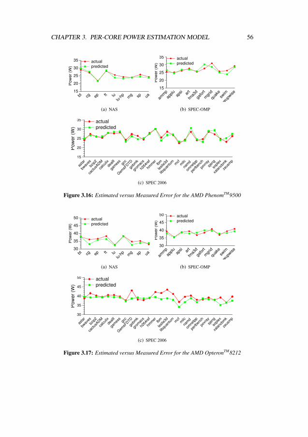
CHAPTER 3. PER-CORE POWER ESTIMATION MODEL 56
bt cg ep ft lulu-h
pm
g sp ua15
20
25
30
35
Po
we
r (W
)
actual
predicted
(a) NAS
amm
p
applu
apsi ar
t
fma3
d
gafo
rt
mgr
id
quak
e
swim
wup
wise
15
20
25
30
35
Po
we
r (W
)
actual
predicted
(b) SPEC-OMP
asta
r
bwav
es
bzip2
cactus
ADM
calculix
dealll
gam
ess
gcc
Gem
sFDTD
gobm
k
grom
acs
h264
ref
hmm
erlbm
leslie3d
libqu
antu
mm
cfm
ilc
nam
d
omne
tpp
perlb
ench
povr
ay
sjen
g
soplex
xalanc
bmk
zeus
mp
15
20
25
30
35
Pow
er
(W)
actual
predicted
(c) SPEC 2006
Figure 3.16: Estimated versus Measured Error for the AMD PhenomTM9500
bt cg ep ft lulu-h
pm
g sp ua30
35
40
45
50
Po
we
r (W
)
actual
predicted
(a) NAS
amm
p
applu
apsi ar
t
fma3
d
gafo
rt
mgr
id
quak
e
swim
wup
wise
30
35
40
45
50
Po
we
r (W
)
actual
predicted
(b) SPEC-OMP
asta
r
bwav
es
bzip2
cactus
ADM
calculix
dealll
gam
ess
gcc
Gem
sFDTD
gobm
k
grom
acs
h264
ref
hmm
erlbm
leslie3d
libqu
antu
mm
cfm
ilc
nam
d
omne
tpp
perlb
ench
povr
ay
sjen
g
soplex
xalanc
bmk
zeus
mp
30
35
40
45
50
Pow
er
(W)
actual
predicted
(c) SPEC 2006
Figure 3.17: Estimated versus Measured Error for the AMD OpteronTM8212

CHAPTER 3. PER-CORE POWER ESTIMATION MODEL 57
bt cg ep ft lulu-h
pm
g sp ua15
20
25
30
35
Po
we
r (W
)
actual
predicted
(a) NAS
amm
p
applu
apsi ar
t
fma3
d
mgr
id
quak
e
swim
wup
wise
15
20
25
30
35
Po
we
r (W
)
actual
predicted
(b) SPEC-OMP
asta
r
bwav
es
bzip2
cactus
ADM
calculix
dealll
gam
ess
gcc
Gem
sFDTD
gobm
k
grom
acs
h264
ref
hmm
erlbm
leslie3d
libqu
antu
mm
cfm
ilc
nam
d
omne
tpp
perlb
ench
povr
ay
sjen
g
soplex
xalanc
bmk
zeus
mp
15
20
25
30
35
Pow
er
(W)
actual
predicted
(c) SPEC 2006
Figure 3.18: Estimated versus Measured Error for the Intel CoreTMi7-870
and/or by using DVFS. We use the power model to compute core power consumptiondynamically. The application spawns one process per core. The scheduler reads PMCvalues via pfmon and feeds the sampled PMC values to the power model to estimate corepower consumption.
The meta-scheduler binds the affinity of the processes to a particular core to simplifytask management and power estimation. It dynamically calculates power values at a setinterval (one second, in our case) and compares the system-power envelope with the sumof power for all cores together with the uncore power.
When the scheduler detects a breach in the power envelope, it takes steps to controlthe power consumption. The scheduler employs two knobs to control system-powerconsumption: dynamic voltage-frequency scaling as a fine knob, and process suspensionas a coarse knob. When the envelope is breached, the scheduler first tries to lower thepower consumption by scaling down the frequency. If power consumption remains toohigh, the scheduler starts suspending processes to meet the envelope’s demands. Thescheduler maintains the record of the power being consumed by the process at the timeof suspension. When the estimated power consumption is less than the target powerenvelope, the scheduler checks whether any of the suspended processes can be resumedbased on the power they were consuming at the time of suspension. If the gap betweenthe current power consumption and the target power budget is not enough to resume asuspended process, and if the processor is operating at a frequency lower than maximum,

CHAPTER 3. PER-CORE POWER ESTIMATION MODEL 58
the scheduler scales up the voltage-frequency. Fig. 3.19 shows the flow diagram of themeta-scheduler.
3.4.1 Sample PoliciesWhen the scheduler suspends a process, it tries to choose the process that will have theleast impact on completion time of all the processes. We explore the use of our powermodel in a scheduler via two sample policies for process suspension.
The Throughput policy targets maximum power efficiency (max instructions/watt)under a given power envelope. When the envelope is breached, the scheduler calculatesthe ratio of instructions/UOPS retired to the power consumed for each core and suspendsthe process having committed the fewest instructions per watt of power consumed. Whenresuming a process, it selects the process (if there is more than one suspended process)that had committed the maximum instructions/watt at the time of suspension. This policyfavors processes that are less often stalled while waiting for load operations to complete.This policy thus favors CPU bound applications.
The Fairness policy divides the available power budget equally among all processes.When applying this policy, the scheduler maintains a running average of the powerconsumed by each core. When the scheduler must choose a process for suspension,it chooses the process having consumed the most average power. For resumption, thescheduler chooses the process that had consumed the least average power at the timeof suspension. This policy strives to regulate core temperature, since it throttles coresconsuming the most average power. Since there is high correlation between core powerconsumption and core temperature, this makes sure that the core with highest tempera-ture receives time to cool down, while cores with lower temperature continue working.Since memory-bound applications are stalled more often, they consume less averagepower, and so this policy favors memory-bound applications.
3.4.2 Experimental SetupFor the scheduler experiments, we use an Intel CoreTMi7-870 system, using DVFS tovary frequencies between 2.926, 2.66, 2.394, 2.128, 1.862, 1.596 and 1.33 GHz. Weform separate power models for different frequencies. The power manager can thusbetter implement policy decisions by estimating power for each frequency. If all corefrequencies have been reduced but the power envelope is still breached, we suspendprocesses to reduce power. We compare against runtimes with no enforced power enve-lope. We divide our workloads into three sets based on CPU intensity. We define CPUintensity as the ratio of instructions retired to last-level cache misses. The three sets

CHAPTER 3. PER-CORE POWER ESTIMATION MODEL 59
Sta
rt
Assig
n o
ne task
per
pro
cessor
Check for
pow
er
envelo
pe b
reach
Envelo
pe
bre
ached?
Suspend a
runnin
g
pro
cess a
s p
er
schedulin
g p
olic
y
Apply
DV
FS
to
low
er
frequency
one s
tep
Low
est
Fre
quency?
Apply
DV
FS
to
incre
ase fre
quency
one s
tep
Resum
e a
suspended
pro
cess a
s p
er
schedulin
g p
olic
y
X m
s D
ela
y
Hig
hest
Fre
quency?
Any p
rocess
suspended?
Yes
No
Yes
No
No
No
Yes
Yes
Figu
re3.
19:F
low
diag
ram
for
the
Met
a-Sc
hedu
ler

CHAPTER 3. PER-CORE POWER ESTIMATION MODEL 60
Benchmark Category Benchmark Applications Peak System Power (W)
CPU-Bound ep, gamess, namd, povray 130
Moderate art, lu, wupwise, xalancbmk 135
Memory-Bound astar, mcf, milc, soplex 130
Table 3.7: Workloads for Scheduler Evaluation
70% 80% 90% 100%
% Power Budget
0
1
2
No
rma
lize
d R
un
Tim
e
Throughput
Fairness
(a) CPU-bound
70% 80% 90% 100%
% Power Budget
0
1
2
No
rma
lize
d R
un
Tim
e
Throughput
Fairness
(b) Memory-bound
70% 80% 90% 100%
% Power Budget
0
1
2
No
rma
lize
d R
un
Tim
e
Throughput
Fairness
(c) Moderate
Figure 3.20: Runtimes for Workloads on the Intel CoreTMi7-870 (without DVFS)
are designated as CPU-Bound, Moderate, and Memory-Bound workloads (in decreasingorder of CPU intensity). The workloads categorized in these sets are listed in Table 3.7.
3.4.3 ResultsFig. 3.20 shows the normalized runtimes for all the workloads when only process sus-pension is used to maintain the power envelope. The Throughput policy should favorCPU-bound workloads, while the Fairness policy should favor memory bound work-loads, but this distinction is not always visible. This is because of the differences in theruntimes of the various workloads. This can be seen from the execution times of theCPU-bound benchmarks when using the Throughput policy. The CPU bound applica-tions ep and gamess have the lowest computational intensities and execution times. Asa result, these two applications are suspended most frequently, which does not affect thetotal execution time, even when the power envelope is set to 80% of peak usage.
Fig. 3.21 shows the results when the scheduler uses both DVFS and process sus-

CHAPTER 3. PER-CORE POWER ESTIMATION MODEL 61
70% 80% 90% 100%% Power Budget
0
1
2
No
rma
lize
d R
un
Tim
e
Throughput
Fairness
(a) CPU-bound
70% 80% 90% 100%
% Power Budget
0
1
2
No
rma
lize
d R
un
Tim
e
Throughput
Fairness
(b) Memory-bound
70% 80% 90% 100%
% Power Budget
0
1
2
No
rma
lize
d R
un
Tim
e
Throughput
Fairness
(c) Moderate
Figure 3.21: Runtimes for Workloads on the Intel CoreTMi7-870 (with DVFS)
pension to maintain the given power envelope. As noted, the scheduler uses DVFS asa fine knob and process suspension as a coarse knob in maintaining the envelope. TheIntel CoreTMi7-870 processor that we use for our experiments supports fourteen differentvoltage-frequency points. These frequency points range from 2.926 GHz to 1.197 GHz.For our experiments, we make models for seven frequency points (2.926, 2.66, 2.394,2.128, 1.862, 1.596 and 1.33 GHz), and we adjust the processor frequency across thesepoints. Our experimental results show that for CPU-bound and moderate benchmarks,there is little difference in execution time under different suspension policies. This sug-gests that for these applications, the scheduler hardly needs to suspend the processes andregulating DVFS points proves sufficient to maintain the power envelope. Performancefor DVFS degrades compared to cases where no DVFS is used. The explanation forthis lies in the difference between runtimes of different applications within the workloadsets. When no DVFS is used, all processes run at full speed. And even when one of theprocesses is suspended, if that process is not critical, it still runs at full speed later inparallel with the critical process. But in the case of DVFS being given higher priorityover process suspension, when the envelope is breached, all processes are slowed, andthis affects total execution time.

CHAPTER 3. PER-CORE POWER ESTIMATION MODEL 62
3.5 Related WorkThe difficulty of obtaining accurate, real-time power measurements together with thegrowing emphasis on green computing have sparked much research on power-estimationmodels. An early effort by Tivari et al. [104] develops a measurement-based approachto model instruction-level power effects. They associate energy cost for each type ofinstruction, instruction pairs and inter-instruction effects like pipeline stalls and cachemisses. They do not distinguish between static and dynamic power components. Theirmethodology requires forming the models separately at each processor frequency.
Russell and Jacome [105] develop simpler models for two members of the Inteli960 R© processor family, finding that detailed per-instruction power information is un-necessary for these processors. Their models are based on measured median averagepower and an estimated power constant.
Like Tivari et al., Cignetti et al. [106] develop models to provide software develop-ers with information on the energy implications of their design decisions. They targetPalmOS R© devices, choosing device power states as their level of abstraction and assum-ing that transitions between states result from system calls. They build system models onthe measured steady-state power of each power state and the power cost of transitioningbetween states.
As the availability and accessibility of hardware performance counters on commod-ity processors increased, more recent power models started utilizing them to build theprocessor power model.
Joseph and Martonosi [48] model power consumption of individual microarchitec-tural components by choosing performance counters that intuitively correlate with com-ponent utilization and deriving weights for each component’s activity factor. They runtheir experiments at a single frequency (since DVFS was not common in 2001) and makeno distinction between static and dynamic power. They cannot estimate power for 24%of the chip, and so they assume peak power for those structures.
Contreras and Martonosi [51] use five PMCs to estimate power for different frequen-cies on an XScale system (with an in-order uniprocessor). They gather data from multi-ple benchmark runs because the number of performance events in their model is greaterthan the number of available counters. They derive power weights for frequency-voltagepairs, and form a parameterized linear model. Their model exhibits low percentage error,like ours, but they test on only seven applications. Unlike our approach, this methodol-ogy is not intended for on-line use.
Economou et al. [42] use PMCs to predict power on a blade server. They profile thesystem using application-independent microbenchmarks. The resulting model estimatespower for the CPU, memory, and hard drive with 10% average error. Their model pro-

CHAPTER 3. PER-CORE POWER ESTIMATION MODEL 63
vides power breakdown between system components but not for on-chip components.Lee and Brooks [54] predict power via statistical inference models. They build
correlations based on hardware parameters, using the most significant parameters to traintheir model. They profile their design space a priori, and then estimate power on randomsamples. This methodology requires training on the same applications for which theywant to estimate power, and so their approach depends on having already sampled allapplications of interest.
Merkel and Bellosa [107] use PMCs to estimate power per processor in an eight-way SMP, shuffling processes to reduce overheating of individual processors. They donot state which PMCs they use, nor how they are chosen. Their goal is not to reducepower, but to distribute it. Their estimation method suffers less than 10% error in a linuxkernel implementation.
The power model presented in this chapter is based on the approach of Singh etal. [52, 68]; we augment that work by porting and validating the model on many plat-forms, improving accuracy of the model by augmenting the microbenchmarks and counterselection methodology, analyzing estimation errors, and exploiting multiple DVFS op-erating points for scheduler validation.
Bertran et al. [50] develop a decomposable model to estimate the power consumedby eight microarchitectural components. Their model relies on 13 performance events.Note that since most processors support counters (two to eight are common), trackingmore events than the number of available counters requires time multiplexing amongthe counters. This reduces observational acuity when sampling, which can contributeto model error. In contrast, both our modeling approaches uses number of performanceevents that are smaller than or equal to the number of available performance counters.
Spiliopoulos et al. [36] use instructions executed and instructions retired counter todevelop a power model. Their model shows high errors for memory-bound benchmarkssince they do not consider memory operations in their model.
The use of power-estimation models for power-aware or energy-aware schedulinghas been explored by various research works.
Isci et al. [39] analyze global power management policies to enforce a given powerbudget and to minimize power consumption for the given performance target. Theyconduct their experiments on the Turandot [108] simulator. They assume the presence ofon-core current sensors to acquire core power information, while they use performancecounters to gather core performance information. They have developed a global powermanager that periodically monitors the power and performance of each core and sets theoperating mode (akin to DVFS performance states) of the core for the next monitoringinterval. They assume that the power mode can be set independently for each core. Theyexperiment with three policies to evaluate their global power manager. The Priority

CHAPTER 3. PER-CORE POWER ESTIMATION MODEL 64
policy assigns different priorities to different cores in a multi-core processor and triesto speed up the core with highest priority while slowing down the lowest priority corewhen the the power consumption overshoots the assigned budget. The policy calledpullHipushLo is similar to our Fairness policy from the above case study; it tries tobalance the power consumption of each core by slowing down the core with highestpower consumption when the power budget is exceeded and speeds up the core withlowest power consumption when there is a power surplus. MaxBIPS tries to maximizethe system throughput by choosing the combination of power modes on different coresthat is predicted to provide maximum overall BIPS (Billion Instructions Per Second).
Rajamani et al. [34] use their power estimation model to drive a power managementpolicy called PerformanceMaximizer. For a given power budget, they exploit the DVFSlevels of the processor to try to maximize the processor performance. For each per-formance state (P-state), they apply their power model to estimate power consumptionat the current P-state. They use the calculated power value to estimate the power con-sumption at other P-states by linearly scaling the current power value with frequency.The scheduler increases the performance state to highest level that it estimates would besafely below the power budget value.
Su et al. [109] use their power model to enforce power capping. They only useDVFS to enforce the power budget while we explore the combination of DVFS and tasksuspension to achieve the power capping requirements.
Banikazemi et al. [38] use a power-aware meta-scheduler. Their meta-schedulermonitors the performance, power and energy of the system by using performance coun-ters and in-built power monitoring hardware. It uses this information to dynamicallyremap the software threads on multi-core servers for higher performance and lower en-ergy usage. Their framework is flexible enough to substitute the hardware power monitorwith a performance-counter based model.
Meng et al. [40] apply a multi-optimization power saving strategy to meet the con-straints of a chip-wide power budget on reconfigurable processors. They run a globalpower manager that configures the CPU frequency and/or cache size of individual cores.They use risk analysis to evaluate the trade-offs between power saving optimizationsand potential performance loss. They select the power-saving strategies at design timeto create a static pool of candidate optimizations. They make an analytic power andperformance model using performance counters and sensors that allows them to quicklyevaluate many power modes and enables their power manager to choose a global powermode at periodic intervals that can obey the processor-wide power budget while maxi-mizing the throughput.
Apart from the work done at the level of individual processor, power-aware strate-gies have also been explored at depth to schedule jobs across multiple nodes in high-

CHAPTER 3. PER-CORE POWER ESTIMATION MODEL 65
performance clusters. Below we discuss few of the related research work.Kim et al. [41] propose scheduling algorithms for bag-of-tasks applications with the
simultaneous aim of meeting deadline constraint and minimizing energy expenditure.They leverage cluster-wide DVFS to implement power-aware scheduling algorithms ontheir simulator.
Ge et al. [110] propose a power-aware runtime system called CPU MISER that im-plements a system-wide power management using DVFS. Their system uses perfor-mance prediction model to achieve a user-specified performance loss constraint whileattempting to reduce energy expenditure.
Marathe et al. [111] develop a power-aware runtime system that aims to maximizeperformance while distributing available power to nodes and cores. Their runtime systemdynamically explores optimal thread concurrency levels and DVFS state to enforce apower budget while simultaneously identifying the critical paths that can be prioritizedduring power budget allocation.
Patki et al. [112] propose a low-overhead resource manager for power-constrainedclusters. They aim to maximize system power utilization by using power-aware schedul-ing algorithms and reduce application turnaround time.
3.6 ConclusionsWe derive statistical, piece-wise multiple linear regression power models mapping PMCvalues and temperature readings to power, and demonstrate their accuracy for the SPEC2006, SPEC-OMP, and NAS benchmark suites. We write microbenchmarks to exercisethe PMCs in order to characterize the machine and run those microbenchmarks with apower meter plugged in to generate data for building the models. For our regressionmodels, we select the PMCs that correlate most strongly with measured power. Be-cause they are built on microbenchmark data, and not actual workload data, the resultingmodels are application independent. We apply the models to 45 benchmarks (includingmultithreaded applications) on five CMPs containing dual- or quad-core chips totalingfour or eight cores. In spite of our generality, estimation errors are consistently lowacross five different systems. We observe overall median errors per machine between1.2% and 4.4%.
We then show the effectiveness of our power model for live power management onan Intel CoreTMsystem with and without DVFS. We suspend and resume processes basedon per-core power usage, ensuring that a given power envelope is not breached. We alsoscale core frequencies to remain under the power envelope.
As numbers of cores and power demands continue to grow, efficient computing re-quires better methods for managing individual resources. The per-core power estimation

CHAPTER 3. PER-CORE POWER ESTIMATION MODEL 66
methodology presented here extends previously published models in both breadth anddepth, and represents a promising tool for helping meet those challenges, both by pro-viding useful information to resource managers and by highlighting opportunities forimproving hardware support for energy-aware resource management. Such support isessential for fine-grained, power-aware resource management.

4Energy Characterization for
Multicore Processors Using Dynamicand Static Power Models
The power modeling methodology presented in Chapter 3 is used to estimate power con-sumption at the granularity of individual cores. This power modeling technique wasshown to be fairly accurate and portable across multiple platforms and also effective forimplementing power budgeting. But a major limitation of this power model was that ithad to be trained separately for each voltage-frequency operating point and hence, in-volves considerable initial investment when the number of individual voltage-frequencyoperating points are in double digits like in modern Intel processors. Moreover, thismodel does not distinguish between core and uncore components of the processor. Theuncore power consumption is equally distributed between the power estimation valuesof individual cores. For the purpose of energy characterization of the microarchitecture,a power model that can provide estimation values at finer granularity would be moreuseful.
Mair et al. [113] emphasize the importance of distinguishing between static and
67

CHAPTER 4. CMP ENERGY CHARACTERIZATION 68
dynamic power due to the fundamental differences in their impact and their parame-ters. Both depend on supply voltage, but static power depends on temperature and dy-namic power depends on frequency. These power components scale differently from onevoltage-frequency step to another, and accurate information on the breakdown betweenthem is critical for understanding energy expenditure trends when applying DVFS.
Another reason to model static and dynamic power separately is to characterize sys-tem energy efficiency. Static power consumption is due to leakage current in the transis-tors, and hence it does not contribute towards performing useful work. The static energythus represents “wasted energy” in the system. The ratio of static to total system en-ergy represents energy inefficiency of the system and can be useful in making qualitativearchitectural comparisons.
We present a systematic methodology for deriving models that calculate static anddynamic power consumption for the uncore and the cores. We show how to isolate andquantify power consumption of different processor components. We validate our powermodels at four different voltage-frequency steps for single-threaded and parallel bench-marks, and show that our models estimate power with good accuracy (mean absoluteerror of 3.14%) across all benchmarks.
We use our models to characterize the energy efficiency of scaling clock frequencythe Haswell processor. We find that uncore static energy represents a significant portionof total system energy (up to 60%), making it a major source of energy inefficiency. Wealso show that running an application at lower frequencies does not always expend lessenergy: the degree to which an application is memory-bound must be considered whenchoosing energy-efficient DVFS policies.
We use the results from energy characterization for frequency scaling to implement alow overhead online DVFS manager and that can switch the system frequency at runtimeto achieve energy-efficiency for the currently running application. We show the efficacyof our DVFS implementation by comparing the energy expenditure and EDP values fromour DVFS runs with those from the runs at best static frequency (chosen after exhausticsearch).
Finally, we use our power models to characterize the energy efficiency of threadscaling on Haswell processor. We identify four orthogonal parameters that affect theperformance and energy efficiency of thread scaling namely, serial fraction, core-to-corecommunication overhead, bandwidth contention and locking mechanism overhead. Weleverage work done previously for characterizing TM systems by Hong et al. [114] tocreate a set of microbenchmarks to vary these four parameters orthogonally and analyzetheir effects on the energy expenditure while varying the number of parallel threads. Wemake different insightful observations and show the level of concurrency at which lowestenergy expenditure is achieved varies based upon the value of identified parameters.

CHAPTER 4. CMP ENERGY CHARACTERIZATION 69
4.1 Power Modeling MethodologyWe run experiments on an Intel Core
TMi7 4770 (Haswell) processor that has four phys-
ical cores with a maximum clock frequency of 3.4 GHz. Each core has two eight-way32 KB private L1 caches (separate I and D), a 256 KB private L2 cache (combined I andD), and an 8 MB shared L3 cache, with 16 GB of physical memory on board.
Since we want to focus on the CPU portion of the chip, our experiments do not usethe on-chip GPU and eDRAM (which are power-gated and cannot affect results). Powermodels for these components would be interesting and useful, but deriving them is be-yond the scope of the work presented here. We disable hyper-threading and Turbo Boostfor all experiments. In the rest of our discussion, we use chip and CPU interchangeably.
We measure power consumption at the ATX CPU power rails using infrastructurethat we built for previous work [115]. This infrastructure uses current transducers toconvert measured current to voltage, which is logged using a data acquisition unit.
We collect performance counter values using the pfmon tool provided by the libpfm4library. We use the Linux R© kernel driver coretemp to read package temperatures viathe on-die Digital Temperature Sensor (DTS) [94].
Our models break total power into four components:
1. uncore dynamic power,
2. core dynamic power,
3. uncore static power, and
4. core static power.
We strive to develop models for each component in isolation in order to prevent modelestimation error of any component from affecting the estimation accuracy of other com-ponents.
4.1.1 Uncore Dynamic Power ModelWe break the uncore dynamic power into uncore idle dynamic power and uncore ac-tive dynamic power. Our experiments indicate that the uncore is neither clock-gatednor power-gated when idle. Eq. 4.1 gives the formula for idle uncore dynamic powerconsumption.
P (uncore)idle_dynamic = α× C × V 2 × F (4.1)

CHAPTER 4. CMP ENERGY CHARACTERIZATION 70
where α = idle uncore activity factor
C = uncore capacitance
V = uncore supply voltage
F = uncore frequency
When idle, the uncore effective capacitance (αC in Eq. 4.1) remains virtually con-stant across frequency changes (we disregard the insignificant uncore activity caused byOS housekeeping threads). Recall that uncore static power depends on uncore voltageand package temperature. We fix uncore voltage from the BIOS and measure idle chippower at the same package temperature at different uncore frequencies. We can thussafely assume that static power remains constant across frequency changes. Any differ-ences in measured power must therefore be due to changes in uncore dynamic power.We measure idle CPU power consumption at frequencies F1 and F2 while making surethat the package temperature is same across two readings. Then, the idle CPU power atuncore frequency Fn can be calculated as Pn = α×C × V 2 × Fn + Pstatic. We thencalculate αC for the idle uncore using Eq. 4.2.
α× C =P2 − P1
V 2F2 − V 2F1(4.2)
Eq. 4.3 shows the model we generate for uncore idle dynamic power. We verify thevalue of αC by repeating our measurements for different values of F1 and F2.
P (uncore)idle_dynamic = 1.41× 10⁻⁹ × V 2 × F (4.3)
where V = uncore supply voltage
F = uncore frequency
We next analyze the effects of L2 cache misses on uncore dynamic power con-sumption. An L2 miss causes activity on the ring interconnect and in the L3 last-levelcache. To measure the effects of L2 misses on CPU power consumption, we create a mi-crobenchmark that interleaves memory accesses with enough integer and floating pointoperations to hide L3 latency. We measure CPU power consumption as we gradually

CHAPTER 4. CMP ENERGY CHARACTERIZATION 71
increase the benchmark’s working-set size such that core activity (micro-operations ex-ecuted per cycle) and L2 activity (L2 requests per cycle) remain constant but the ratioof L2 misses to L2 requests increases. We attribute differences in consumed power toincreases in uncore activity from the increased L2 misses. We run regression analysison the L2 miss rate and increase in power consumption to generate a quadratic modelfor the L2-miss contribution to uncore dynamic power. Eq. 4.4 shows this model, andFigure 4.1 shows its accuracy with respect to our measured values. The R2 coefficientmeasuring the goodness of the fit for the estimation model is 0.999.
P (uncore)L2_miss_dynamic = (3.043× 10⁻⁹ × x2
+ 2.881× 10⁻⁹ × x)
× V 2 × F
(4.4)
where x = chip-wide L2 misses per uncore cycle
V = uncore supply voltage
F = uncore frequency
0.0 0.1 0.2 0.3
L2 Misses/Cycle
0.0
0.1
0.2
0.3
0.4
Pow
er
(W)
Estimated
Measured
Figure 4.1: Model Fitness for Power Consumed due to L2 Misses at F=800 MHz and
V=0.7V
We perform a similar experiment to measure effects of L3 misses on uncore power.For realistic L3 miss rates (≤ 50 MPKI), CPU power consumption increases by less than0.5 W even though DRAM power consumption increases significantly. Our models thusomit L3 misses, and we compute total uncore dynamic power consumption as the sumof uncore idle dynamic power and uncore power due to L2 misses.

CHAPTER 4. CMP ENERGY CHARACTERIZATION 72
4.1.2 Core Dynamic Power ModelTo model core dynamic power consumption, we study the effects of microarchitecturalevents like micro-operations (uops) executed, L1 accesses, and L2 accesses. We start byquantifying the effects of non-memory operations on core dynamic power. We wouldprefer to analyze integer and floating point operations separately, but the Haswell mi-croarchitecture provides no performance counter for floating point operations. We thusaverage over both instruction types. We create microbenchmarks that loop over the fol-lowing instructions, alone and in combination:
• x87 floating point multiplications,
• x87 floating point additions,
• integer multiplications,
• integer additions,
• SIMD floating-point multiplications, and
• SIMD floating-point additions.
For each microbenchmark, we calculate αC using the same technique as for cal-culating idle uncore power: we fix uncore voltage, uncore frequency, and core voltagefrom the BIOS. We then initiate microbenchmark execution on all cores, measure powerconsumption, switch the cores to a higher frequency, and measure again within 10 ms.
Since the uncore voltage, uncore frequency, and package temperature are stableacross readings (assuming that temperature change is insignificant within the very smallsampling period), the difference in measured power must be due to changes in core dy-namic power consumption. αC can now be calculated using Eq. 4.2. We calculate αCfor multiple frequency pairs and take an average to reduce estimation error. We followthis approach to calculate αC for all microbenchmarks. We use linear regression tofind the best fit for estimating the impact of non-memory instructions on core dynamicpower. Eq. 4.5 shows the derived model, and Figure 4.2 shows its fitness with respect toour measured values. The R2 fitness coefficient is 0.801.
P (core)non−mem_dynamic =(2.448× 10⁻¹⁰ × x+
1.181× 10⁻⁹)× V 2 × F(4.5)
where x = Non-memory instructions per cycle
V = core supply voltage
F = core frequency
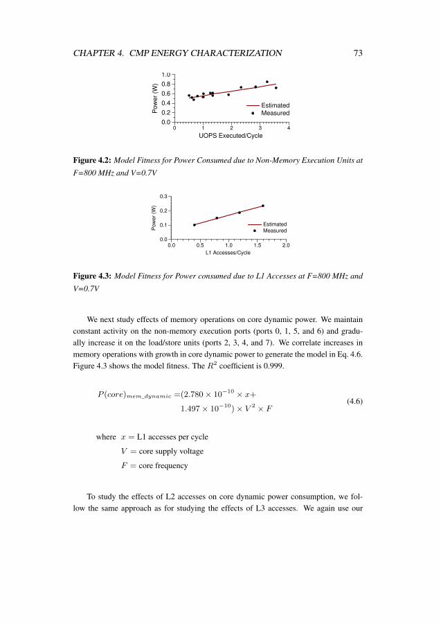
CHAPTER 4. CMP ENERGY CHARACTERIZATION 73
0 1 2 3 4
UOPS Executed/Cycle
0.0
0.2
0.4
0.6
0.8
1.0
Pow
er
(W)
Estimated
Measured
Figure 4.2: Model Fitness for Power Consumed due to Non-Memory Execution Units at
F=800 MHz and V=0.7V
0.0 0.5 1.0 1.5 2.0
L1 Accesses/Cycle
0.0
0.1
0.2
0.3
Po
we
r (W
)
Estimated
Measured
Figure 4.3: Model Fitness for Power consumed due to L1 Accesses at F=800 MHz and
V=0.7V
We next study effects of memory operations on core dynamic power. We maintainconstant activity on the non-memory execution ports (ports 0, 1, 5, and 6) and gradu-ally increase it on the load/store units (ports 2, 3, 4, and 7). We correlate increases inmemory operations with growth in core dynamic power to generate the model in Eq. 4.6.Figure 4.3 shows the model fitness. The R2 coefficient is 0.999.
P (core)mem_dynamic =(2.780× 10⁻¹⁰ × x+
1.497× 10⁻¹⁰)× V 2 × F(4.6)
where x = L1 accesses per cycle
V = core supply voltage
F = core frequency
To study the effects of L2 accesses on core dynamic power consumption, we fol-low the same approach as for studying the effects of L3 accesses. We again use our

CHAPTER 4. CMP ENERGY CHARACTERIZATION 74
microbenchmark to increase the number of L2 accesses while keeping core activity con-stant. We measure the increase in CPU power consumption as we increase the L2 accessrate. We then run linear regression on the L2 access rate and increase in power con-sumption to generate the model for the L2-access contribution to core dynamic powerconsumption shown in Eq. 4.7. Figure 4.4 shows the model fitness with respect to ourmeasured values. The R2 coefficient that measures the goodness of the fit is 0.997.
P (core)L2_dynamic = 2.829× 10⁻⁹ × x× V 2 × F (4.7)
where x = per-core L2 accesses per uncore cycle
V = uncore supply voltage
F = uncore frequency
0.00 0.05 0.10 0.15 0.20
L2 Accesses/Cycle
0.0
0.1
0.2
0.3
Pow
er
(W)
Estimated
Measured
Figure 4.4: Model Fitness for Power Consumed due to L2 Accesses at F=800 MHz and
V=0.7V
The total core dynamic power consumption can now be expressed by Eq. 4.8.
P (core)dynamic = P (core)mem_dynamic+
P (core)non−mem_dynamic+
P (core)L2_dynamic
(4.8)
4.1.3 Uncore Static Power ModelThe Haswell microarchitecture uses a deep-sleep C-state, C7, when a core is idle. In theC7 state, the cores are power-gated, and so they consume negligible power. In contrast,our experiments show that the Haswell uncore is neither power-gated nor clock-gated

CHAPTER 4. CMP ENERGY CHARACTERIZATION 75
when the chip is idle. The idle power consumption of the chip is thus almost entirelydue to the uncore. Chip idle power can be expressed by Eq. 4.9.
P (CPU)idle =P (uncore)idle_dynamic+
P (uncore)static(4.9)
We use the model for P (uncore)idle_dynamic derived in Section 4.1.1 to isolateP (uncore)static. Recall that static power consumption depends on supply voltage andtemperature. We use CPU package temperature to approximate average temperatureacross the uncore. To measure effects of uncore voltage and uncore temperature on un-core static power, we set the uncore voltage to values ranging from 0.7V to 1.0V withincrements of 0.05V. At each voltage, we vary CPU temperature using a hot-air gun, andwe measure power consumption at the granularity of one sample per second. We subtractuncore idle dynamic power from the measured values and run non-linear regression onthis difference, the voltage, and the temperature to create the uncore static power modelin Eq. 4.10. This equation is based upon the Poole-Frenkel effect [116] which providesa generic equation for current density through an electrical insulator. We use this equa-tion simply as a base equation for curve-fitting and do not claim to estimate technologyconstants based upon the values acquired from non-linear regression. Figure 4.5 showsmeasured versus estimated uncore static values at three voltage points. We ran eachexperiment until temperature stopped dropping (the figure shows time windows of 200seconds for ease of comparison — experiments that ran longer continued to show highestimation accuracy during the time not shown). The R2 coefficient for the estimationmodel is 0.999 across all sample points.
P (uncore)static = A× e−(−169.083+1202.02×√V
273.15+T) × V 2 (4.10)
where V = uncore supply voltage
T = package temperature
4.1.4 Core Static Power ModelTo generate a model for core static power, we force the core to remain in state C0. In thisstate, the Linux kernel runs a polling idle loop that consumes constant dynamic power.We calculate this power with the same strategy we used to calculate uncore idle dynamic

CHAPTER 4. CMP ENERGY CHARACTERIZATION 76
0 50 100 150 200
Time (s)
0
2
4
6
8
Po
we
r (W
)
measured
estimated
0
20
40
60
80
Te
mp
era
ture
(C)
temp
(a) V=0.70
0 50 100 150 200
Time (s)
0
2
4
6
8
Po
we
r (W
)
0
20
40
60
80
Te
mp
era
ture
(C)
(b) V=0.85
0 50 100 150 200
Time (s)
0
2
4
6
8
Po
we
r (W
)
0
20
40
60
80
Te
mp
era
ture
(C)
(c) V=1.0
Figure 4.5: Uncore Static Model Fitness
power. We calculate αC for idle cores in state C0 using Eq. 4.2. Eq. 4.11 shows themodel for per-core dynamic power in state C0. Eq. 4.12 uses Eq. 4.11 to isolate per-corestatic power consumption.
P (core)C0_dynamic = 1.28× 10⁻⁹ × V 2 × F (4.11)
where V = core supply voltage
F = core frequency
P (core)static =1
4× (P (CPU)C0 − P (uncore)idle_dynamic
− P (uncore)static − 4× P (core)C0_dynamic)(4.12)
To create the core static power model we first measure the effects of core voltage andtemperature. We use package temperature as an approximation for core temperature. Wefix cache voltage at 0.7V and frequency at 800 MHz from the BIOS. We again incremen-tally increase core voltage from 0.7V to 1.05V in steps of 0.05V. At each voltage, we

CHAPTER 4. CMP ENERGY CHARACTERIZATION 77
0 50 100 150 200 250 300 350
Time (s)
0
2
4
6
8
Po
we
r (W
)
measured
estimated
0
20
40
60
80
Te
mp
era
ture
(C)
temp
(a) V=0.70
0 50 100 150 200 250 300 350
Time (s)
0
2
4
6
8
Po
we
r (W
)
0
20
40
60
80
Te
mp
era
ture
(C)
(b) V=0.85
0 50 100 150 200 250 300 350
Time (s)
0
2
4
6
8
Po
we
r (W
)
0
20
40
60
80
Te
mp
era
ture
(C)
(c) V=1.0
Figure 4.6: Core Static Model Fitness
vary package temperature using a hot-air gun, and we measure changes in power con-sumption and temperature. We run non-linear regression on collected data to create thecore static model in Eq. 4.13. Figure 4.6 shows measured versus estimated core staticvalues at three voltage points. The estimated model fits measured values with an R2
coefficient of 0.996.
P (core)static = 1525.07× e−( 1884.1+525.556×√V
273.15+T) × V 2 (4.13)
where V = core supply voltage
T = package temperature
4.1.5 Total Chip Power ModelBased on our findings, we must consider two more components in constructing a full-chip power model.

CHAPTER 4. CMP ENERGY CHARACTERIZATION 78
First, our measurements show that when core frequency is increased, chip powerconsumption increases more than expected at certain frequency steps. These increasesappear to depend on the number of active cores but not on core activity. We believe thisphenomenon is due to the core PLL switching to higher supply voltages above certainfrequencies. An example of this unexpected increase in power is shown in Figure 4.7.We take following steps to conduct this experiment:
1. Fix core and uncore voltage to 1.0V (from BIOS).
2. Fix uncore frequency to 800 MHz (from BIOS).
3. Fix C-state for all cores to C0 (active).
4. Set power measurement equipment to take samples every millisecond.
5. Set core frequency to 800 MHz.
6. Keep cores idle for 50 ms.
7. Switch to next higher frequency for 10 ms.
8. Repeat steps 5 to 7 for all available frequencies.
Figure 4.7: Abrupt Jump in Power Consumption at Higher Frequency
When the core frequency is switched, the temperature is not expected to changesignificantly due to small time duration (10ms) during which the higher frequency wasenabled. Moreover the uncore voltage and frequency was fixed for the duration of theexperiment. Hence, the change in in power consumption observed in the experimentsis almost entirely due to change in core dynamic power consumption. Since the corevoltage was also fixed from BIOS, we expect to see an almost linear rise in power con-sumption as frequency is increased. But as seen in Figure 4.7, this is true to till certain
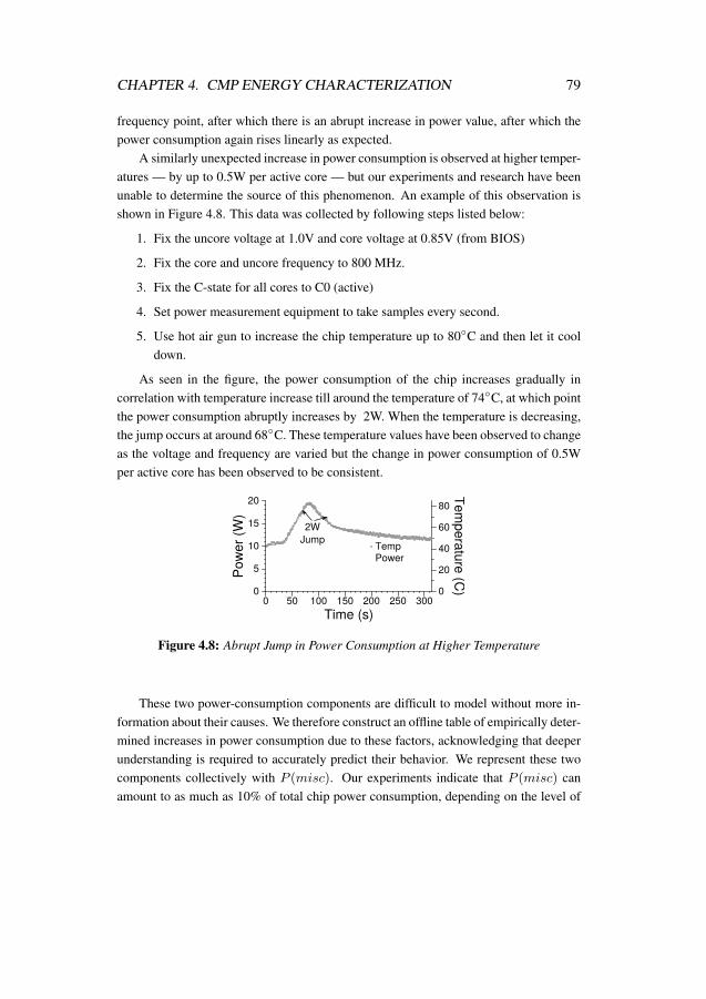
CHAPTER 4. CMP ENERGY CHARACTERIZATION 79
frequency point, after which there is an abrupt increase in power value, after which thepower consumption again rises linearly as expected.
A similarly unexpected increase in power consumption is observed at higher temper-atures — by up to 0.5W per active core — but our experiments and research have beenunable to determine the source of this phenomenon. An example of this observation isshown in Figure 4.8. This data was collected by following steps listed below:
1. Fix the uncore voltage at 1.0V and core voltage at 0.85V (from BIOS)
2. Fix the core and uncore frequency to 800 MHz.
3. Fix the C-state for all cores to C0 (active)
4. Set power measurement equipment to take samples every second.
5. Use hot air gun to increase the chip temperature up to 80◦C and then let it cooldown.
As seen in the figure, the power consumption of the chip increases gradually incorrelation with temperature increase till around the temperature of 74◦C, at which pointthe power consumption abruptly increases by 2W. When the temperature is decreasing,the jump occurs at around 68◦C. These temperature values have been observed to changeas the voltage and frequency are varied but the change in power consumption of 0.5Wper active core has been observed to be consistent.
0
20
40
60
80
Temperature (C
)
Temp
0 50 100 150 200 250 300Time (s)
0
5
10
15
20
Pow
er (W
)
Power
2WJump
Figure 4.8: Abrupt Jump in Power Consumption at Higher Temperature
These two power-consumption components are difficult to model without more in-formation about their causes. We therefore construct an offline table of empirically deter-mined increases in power consumption due to these factors, acknowledging that deeperunderstanding is required to accurately predict their behavior. We represent these twocomponents collectively with P (misc). Our experiments indicate that P (misc) canamount to as much as 10% of total chip power consumption, depending on the level of

CHAPTER 4. CMP ENERGY CHARACTERIZATION 80
Suite Benchmarks
NAS SP, EP, BT, MG, DC, UA, CG
SPEC OMP2001quake, swim, wupwise, ammp,
apsi, applu, mgrid
SPEC CPU2006
cactusADM, calculix, dealII, gamess,GemsFDTD, gromacs, lbm, leslie3d, milc,
namd, povray, soplex, zeusmp, astar, bzip2,gcc, gobmk, h264ref, hmmer, libquantum, mcf,
omnetpp, perlbench, sjeng, xalancbmk
Table 4.1: Benchmarks Used for Validation
core and uncore activity. Total chip power consumption is then given as:
P (CPU) = P (uncore)dynamic + P (uncore)static
+ P (core)dynamic + P (core)static + P (misc)(4.14)
4.2 ValidationWe validate our power models on the single-threaded SPEC CPU2006 [96] benchmarks,NAS Parallel Benchmarks [99], and multithreaded SPEC OMP2001 [97] applications inTable 4.1. We omit bwaves from SPEC CPU2006 and art and fma3d from SPEC OMP2001because they do not run on our system. We use the NAS class B inputs, and we omit ISbecause it does not run for long enough time periods to gather reliable measurements.We run the parallel applications with one, two, and four threads. Similarly, we run one,two, and four concurrent instances of the sequential applications. Once per second weread package temperature and core voltage, and collect performance counter as describedin Section 4.1. We measure processor power every 1 ms and average the values over onesecond to sync the power values with other parameters. To verify that our model esti-mates power accurately across different voltage-frequency steps, we validate it at fourDVFS points: 800 MHz at 0.7V, 1500 MHz at 0.78V, 2400 MHz at 0.88V, and 3400MHz at 1.01V.
Figure 4.9 shows estimation error for our benchmark suites. Mean absolute error(MAE) for all NAS benchmarks across the four DVFS points is 3.19% for a single thread,1.89% for two threads, and 2.50% for four threads. MAE for SPEC CPU2006 is 3.88%for single-instance runs, 2.74% for double-instance runs, and 2.60% for quad-instanceruns. MAE for SPEC OMP2001 is 3.79% for a single thread, 2.87% for two threads, and3.42% for four threads. Mean absolute error across all sample points for all benchmarksand voltage-frequency states is 3.14%, and the standard deviation is 2.87%.
Our model predicts power estimation with good accuracy for most benchmarks. For

CHAPTER 4. CMP ENERGY CHARACTERIZATION 81
800
MHz
1.25
GHz
2.4
GHz
3.4
GHz All
0
2
4
6
% M
ean E
rror
(Sta
ndard
Devia
tion)
1 Thread2 Threads4 ThreadsStd Dev
(a) NAS Parallel Benchmarks
800
MHz
1.25
GHz
2.4
GHz
3.4
GHz All
0
2
4
6
% M
ean E
rror
(Sta
ndard
Devia
tion)
(b) SPEC CPU2006
800
MHz
1.25
GHz
2.4
GHz
3.4
GHz All
0
2
4
6
% M
ean E
rror
(Sta
ndard
Devia
tion)
(c) SPEC OMP2001
Figure 4.9: Validation of Total Chip Power
the benchmarks with rapid phase changes (DC in NAS and ammp in SPEC OMP2001),we had to re-run the validation experiments at the higher measurement granularity of100 ms to accurately estimate their rapidly changing power consumption values.
We know that model error arises from at least two sources. First, the Haswell mi-croarchitecture provides no per-core event to track executed floating point operations,which prevents us from creating separate models for floating point and integer instruc-tion executions. This creates slight model inaccuracies for compute-intensive phases.Second, values in the offline table we create to account for P (misc) are not always ac-curate, especially at higher frequencies during periods of rapid phase change. Despitethese known sources of error, our model accurately predicts workload energy trendswhen scaling both frequency and numbers of threads.
4.3 Energy Characterization of Frequency ScalingDynamic voltage-frequency scaling permits hardware or software to adjust clock speed(and voltage) in an attempt to trade-off performance for energy. However, finding thefrequencies at which an application meets performance goals while maintaining a givenenergy budget is not necessarily straightforward. We use our power models to charac-terize energy efficiency by showing how static and dynamic energy from the core anduncore components scale in conjunction with DVFS.
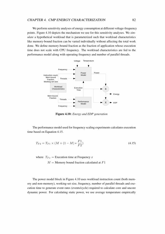
CHAPTER 4. CMP ENERGY CHARACTERIZATION 82
We perform sensitivity analyses of energy consumption at different voltage-frequencypoints. Figure 4.10 depicts the mechanism we use for this sensitivity analyses. We sim-ulate a hypothetical workload that is parameterized such that workload characteristicslike memory-bound fraction can be varied individually without affecting the total workdone. We define memory-bound fraction as the fraction of application whose executiontime does not scale with CPU frequency. The workload characteristics are fed to theperformance model along with operating frequency and number of parallel threads.
WorkloadCharacteristics
PowerModel
PerformanceModel
Instruction count,Mem-bound
Fraction,Working-set size
Threads
Frequency
Voltage Temperature
Execution Time
Frequency
Threads
Mem-bound Fraction
X
Power
Energy
EDPX
Figure 4.10: Energy and EDP generation
The performance model used for frequency scaling experiments calculates executiontime based on Equation 4.15.
TF2 = TF1 × (M + (1−M) ∗ F1
F2) (4.15)
where TFx = Execution time at Frequency x
M = Memory bound fraction calculated at F1
The power model block in Figure 4.10 uses workload instruction count (both mem-ory and non-memory), working-set size, frequency, number of parallel threads and exe-cution time to generate event rates (events/cycle) required to calculate core and uncoredynamic power. For calculating static power, we use average temperature empirically

CHAPTER 4. CMP ENERGY CHARACTERIZATION 83
observed across all benchmarks at each combination of DVFS operaring point and num-ber of active cores. The power value generated by the power model is multiplied withthe execution time generated by the performance model to calculate energy, which inturn is multiplied by the execution time to generate energy-delay product (EDP).
4.3.1 Energy Effects of DVFSWe first examine how voltage-frequency scaling affects energy consumption. Conven-tional wisdom says that running at higher frequencies boosts performance at the expenseof expending more energy [109] because dynamic power scales quadratically with volt-age (Eq. 4.1). But when we take into account the effects of energy consumed by theuncore, we find that running at a lower voltage-frequency step can sometimes expendmore energy. Figure 4.11 shows how energy scales for our synthetic workload as wevary its memory-bound fraction and the frequency at which we execute. Energy num-bers are normalized to the energy expenditure at the lowest frequency (800 MHz). Wemake following observations from these results.
Observation 1: The frequency at which lowest energy is expended depends on thememory-bound fraction of the application.
Explanation: At the lowest frequency for single-threaded run, the uncore energyaccounts for 74% of the total. Specifically, uncore static energy constitutes 61% of thetotal energy expenditure. Increasing the CPU frequency reduces execution time and thisresults in reduction of uncore static energy. But increasing frequency increases core anduncore dynamic energy because of the quadratic relationship between dynamic powerand voltage. The extent to which the performance scales with frequency depends on thememory-bound fraction of the application as per Equation 4.15. If the performance gainachieved by increasing frequency is large enough, the reduction in uncore static energyoffsets the gain in dynamic energy resulting in overall reduction in total energy. This iswhat we see in Figure 4.11(a) when the frequency is increased from 800 MHz to 1500MHz when memory-bound fraction is less than 40%. After a certain frequency, increasesin (core and uncore) dynamic energy dwarf reduction in uncore static energy, causingtotal energy expenditure to rise again. The more memory-bound an application, the lessperformance it gains from running at higher frequencies, and so reductions in uncorestatic energy become less significant with increasing frequency. When the memory-bound portion of a single-threaded application exceeds 40%, we see the expected trend:increasing the frequency increases energy expenditure.
Observation 2: There is a significant difference between the energy trends forsingle-threaded run and four-threaded runs. For example, at 0% memory-boundedness,the least energy is expended at 2.4 GHz for single-threaded runs and 1.5 GHz for four-

CHAPTER 4. CMP ENERGY CHARACTERIZATION 84
threaded runs.Explanation: When more cores are active on the processor instead of one, at any
given instant, the ratio of core power to total chip power is higher than the case whenonly one core is active. As a result, the uncore static energy is less significant for multi-threaded, CPU-bound applications (we measure 49% at two threads and 35% at fourthreads for 0% memory-bound). Consequently, when the frequency is increased formulti-threaded runs, the increase in core dynamic energy offsets the decrease in uncorestatic energy at lower memory-bound fractions compared to single-threaded runs. Theenergy scaling correlates with frequency scaling when a two-thread application is 30%memory-bound and a four-thread application is 20% memory-bound (compared to 40%for a single-threaded application).
800
MHz
1.5
GHz
2.4
GHz
3.4
GHz
800
MHz
1.5
GHz
2.4
GHz
3.4
GHz
800
MHz
1.5
GHz
2.4
GHz
3.4
GHz
800
MHz
1.5
GHz
2.4
GHz
3.4
GHz
800
MHz
1.5
GHz
2.4
GHz
3.4
GHz
800
MHz
1.5
GHz
2.4
GHz
3.4
GHz
800
MHz
1.5
GHz
2.4
GHz
3.4
GHz
0
0.5
1.0
1.5
2.0
2.5
No
rma
lize
d E
ne
rgy (
Tim
e)
Uncore Dynamic EnergyUncore Static EnergyCore Dynamic EnergyCore Static EnergyExecution Time
0% 10% 20% 30%
Memory Boundedness
40% 50% 100%
(a) 1 Thread
800
MHz
1.5
GHz
2.4
GHz
3.4
GHz
800
MHz
1.5
GHz
2.4
GHz
3.4
GHz
800
MHz
1.5
GHz
2.4
GHz
3.4
GHz
800
MHz
1.5
GHz
2.4
GHz
3.4
GHz
800
MHz
1.5
GHz
2.4
GHz
3.4
GHz
800
MHz
1.5
GHz
2.4
GHz
3.4
GHz
800
MHz
1.5
GHz
2.4
GHz
3.4
GHz
0
0.5
1.0
1.5
2.0
2.5
No
rma
lize
d E
ne
rgy (
Tim
e)
0% 10% 20% 30%
Memory Boundedness
40% 50% 100%
(b) 4 Threads
Figure 4.11: Effects of DVFS on Total Energy and Performance
This analysis shows that the extent to which an application is memory bound mustbe taken into account when choosing a frequency at which to run the application suchthat it expends the least energy. We repeated our frequency scaling experiments whilevarying the workload characteristics like instruction mix and working-set size and cameto conclusion that relationship between frequency and energy efficiency for any work-load is only affected by the memory bound fraction of the workload and the number of

CHAPTER 4. CMP ENERGY CHARACTERIZATION 85
parallel threads.
4.3.2 DVFS PredictionThe energy characterization of frequency scaling discussed in Section 4.3.1 underscoresthe importance of running either entire applications or their individual phases at appro-priate frequencies to reduce system’s energy expenditure. In this section, we leveragethe the energy characterization done in that section to propose an online DVFS managerfor energy-efficient frequency scaling. Prior works that leverages power modeling forimplementing online DVFS manager [36, 109] propose the following approach:
1. Define a fixed scheduling quantum (for example, 10 ms).
2. Fix the system frequency for the current quantum.
3. Track performance events required to calculate power consumption at the cur-rently chosen frequency.
4. At the end of the scheduling quantum, feed the collected statistics to the chosenenergy model to predict energy at all the DVFS operating points for the systemassuming that application would maintain similar behavior for the next quantum.
5. Set the system frequency to value that is predicted to expend least energy/EDP inthe above step.
6. Repeat steps 3 to 5 at the end of every scheduling quantum.
This approach is shown to work well but requires power model calculations for eachavailable system frequency at every scheduling quantum incurring energy overheads ofits own. For example, on our Haswell processor there are sixteen different available fre-quency points available. This means that making frequency prediction for DVFS man-agement would require sixteen energy calculations at every scheduling interval. Thisputs a constraint on how small the scheduling interval can be without incurring signifi-cant power and/or performance overhead of doing power calculations. We show in thissection a much simpler approach to selecting the energy-efficient frequency, one thatdoes not require such extensive calculations and is equally effective.
Figure 4.11 shows that the DVFS operating point at which a particular applicationwill expend lowest energy is a function of an application’s memory boundedness andthe number of active cores. The memory boundedness of an application is a functionof number of LLC misses, the LLC miss latency in terms of core cycles, and its effecton the application’s execution time due to stalls in processor pipeline caused by datadependencies on LLC misses. The memory-bound fraction of the application can be for-mulated as the ratio of cycles during which execution was stalled due to LLC misses to

CHAPTER 4. CMP ENERGY CHARACTERIZATION 86
total execution time in cycles. In an out-of-order processor, it is difficult to isolate execu-tion stalls caused specifically by LLC misses from other overlapping stalls from eventslike branch mispredictions, the load/store queue getting full, or miss penalties from dataaccesses to lower-level caches. Due to this limitation, we must approximate the num-ber of pipeline stalls caused by LLC misses. The Haswell microarchitecture supportsa performance event named CYCLE_ACTIVITY:STALLS_L2_PENDING, which countsthe number of core cycles during which the execution is stalled and an L2 miss is wait-ing to be served. It should be noted that this counter may not necessarily provide anexact count of execution stall cycles due to L2 misses, since it is possible that some ofthe stall cycles during a pending L2 miss were due to branch mispredictions. But giventhe high accuracy of modern branch predictors, we consider this event to be a good ap-proximation of L2 miss stall cycles. From this event, we can estimate the L3 miss stallcycles using Equation 4.16. The L3 miss ratio in this equation is the ratio of memoryloads that miss in L3 to total memory load operations retired. We consider only loadsin this equation because store misses are not in the critical path of execution in modernout-of-order processors.
L3Miss Stall Cycles =
CY CLE_ACTIV ITY : STALLS_L2_PENDING
× L3Miss Ratio
(4.16)
The memory-bound fraction can then be calculated using Equation 4.17.
Mem Bound Fraction =L3Miss Stall Cycles
Total Cycles(4.17)
CyclesF2 = CyclesF1 × (1−M +M ∗ F2
F1) (4.18)
where CyclesFx = Execution time in cycles at Frequency x
M = Memory bound fraction calculated at F1
Overall, we must track the four performance events listed in Table 4.2 for calculatingthe memory-bound fraction of an application. To validate the accuracy of Equation 4.17,we run the benchmarks in Table 4.1 (at one, two, and four threads) at one frequency

CHAPTER 4. CMP ENERGY CHARACTERIZATION 87
Performance Event Description
UNHALTED_CORE_CYCLES Core cyclesMEM_LOAD_UOPS_RETIRED:L3_HIT Memory loads that hit L3MEM_LOAD_UOPS_RETIRED:L3_MISS Memory loads that miss L3CYCLE_ACTIVITY:STALLS_L2_PENDING Pipeline stalls during L2 miss pending
Table 4.2: Performance events required to calculated memory bound
Parameter Values
Frequency (GHz)0.8, 1.0, 1.1, 1.3, 1.5, 1.7, 1.8, 2.0,2.2, 2.4, 2.5, 2.7, 2.9, 3.1, 3.2, 3.4
Threads 1, 2, 4
Mem-bound %0, 5, 10, 15, 20, 25, 30, 35, 40, 45,
50, 55, 60, 65, 70, 75, 80, 85, 90, 95, 100
Table 4.3: Parameter Values Used for Generating Energy Numbers
and use the calculated memory bound to predict execution time at different frequenciesusing Equation 4.18. When we predict performance from 3.4 GHz to 800 MHz, themean absolute error across benchmarks is 3.35%, with a standard deviation of 3.81%.When the performance is predicted from 800 MHz to 3.4 GHz, the mean absolute erroris 6.58%, with a standard deviation of 6.37%. The prediction error increases for 800MHz because some LLC-induced pipeline stalls that occur at higher frequencies maydisappear at lower frequencies.
Our validation for performance prediction shows that we can predict the memory-bound fraction at any frequency with reasonable accuracy. This, in turn, means that wecan predict the frequency at which the current application phase will be most energy-efficient by just tracking the events required to calculate the memory-bound fraction,instead of tracking all events required to calculate power consumption.
We repeat the methodology from Section 4.3.1, where we use the power models for-mulated for our system to calculate energy for a hypothetical workload while varyingthe core frequency, number of parallel threads, and the workload’s memory-bound frac-tion. Table 4.3 lists the values of these three parameters that we use in our experiments.After predicting energy and EDP values at each combination of frequency, threads, andmemory-bound fraction, we are able to determine the frequency at which a workload(or an individual phase) will expend the least energy/EDP. We populate a table with thisinformation. An online DVFS manager can then simply use this table to predict the mostenergy-efficient voltage-frequency point for the current phase based on the calculatedmemory bound percentage, without the need to predict energy at all available systemfrequencies. This reduces the overhead associated with DVFS management while stillretaining accurate energy-efficient frequency predictions.

CHAPTER 4. CMP ENERGY CHARACTERIZATION 88
To validate this DVFS prediction methodology, we run benchmarks from Table 4.1at all system frequencies to find the frequency at which the benchmark expends leastenergy (hereafter termed FE). We then calculate the average memory-bound fraction ofthe application from the performance events collected at 3.4 GHz. Based on the calcu-lated memory-bound fraction, we predict the frequency at which the benchmark wouldexpend least energy (hereafter P (3.4)E) and compare the prediction with the empiri-cally determined best frequency (FE). We repeat the same experiment by calculatingthe memory-bound fraction at 800 MHz and predicting the lowest energy frequency(P (0.8)E). Figure 4.12 compares the predicted frequency versus actual frequency forthe NAS benchmarks at which least energy is expended. Since the memory-bound frac-tion changes when the frequency changes, and because of the error in calculating mem-ory boundedness, the predicted frequencies from 800 MHz and 3.4 GHz are not alwaysthe same. However, these two predictions are very close to the actual lowest energyfrequency for almost all benchmarks. Figure 4.13 shows the energy expenditure at pre-dicted frequencies normalized to energy expenditure at FE . The error in frequency pre-diction results in an average of around 5% increase in energy expenditure across thebenchmarks.
EP SP CG UA MG LU FT BT0
500
1000
1500
2000
2500
Fre
qu
en
cy (
MH
z)
Prediction (3.4 GHz)
Prediction (800 MHz)
Actual
(a) 1 Thread
EP SP CG UA MG LU FT BT0
500
1000
1500
2000
2500
Fre
qu
en
cy (
MH
z)
Prediction (3.4 GHz)
Prediction (800 MHz)
Actual
(b) 2 Threads
EP SP CG UA MG LU FT BT0
500
1000
1500
2000
2500
Fre
qu
en
cy (
MH
z)
Prediction (3.4 GHz)
Prediction (800 MHz)
Actual
(c) 4 Threads
Figure 4.12: Actual versus predicted frequency at which least energy is expended for
NAS benchmarks
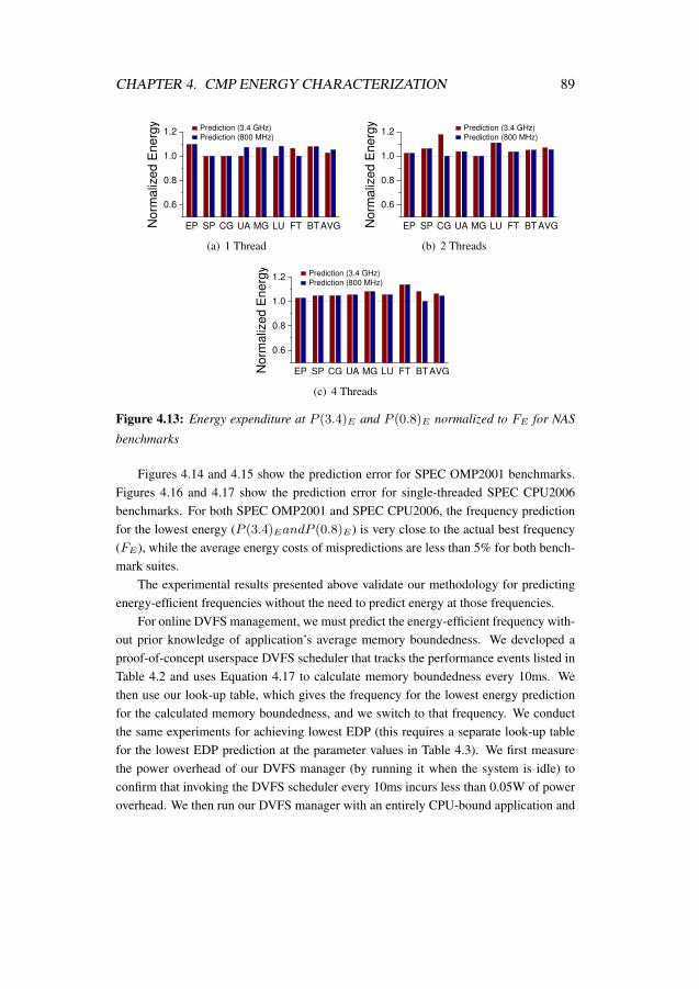
CHAPTER 4. CMP ENERGY CHARACTERIZATION 89
EP SP CG UA MG LU FT BTAVG
0.6
0.8
1.0
1.2
Norm
aliz
ed E
nerg
y Prediction (3.4 GHz)
Prediction (800 MHz)
(a) 1 Thread
EP SP CG UA MG LU FT BTAVG
0.6
0.8
1.0
1.2
Norm
aliz
ed E
nerg
y Prediction (3.4 GHz)
Prediction (800 MHz)
(b) 2 Threads
EP SP CG UA MG LU FT BTAVG
0.6
0.8
1.0
1.2
Norm
aliz
ed E
nerg
y Prediction (3.4 GHz)
Prediction (800 MHz)
(c) 4 Threads
Figure 4.13: Energy expenditure at P (3.4)E and P (0.8)E normalized to FE for NAS
benchmarks
Figures 4.14 and 4.15 show the prediction error for SPEC OMP2001 benchmarks.Figures 4.16 and 4.17 show the prediction error for single-threaded SPEC CPU2006benchmarks. For both SPEC OMP2001 and SPEC CPU2006, the frequency predictionfor the lowest energy (P (3.4)EandP (0.8)E) is very close to the actual best frequency(FE), while the average energy costs of mispredictions are less than 5% for both bench-mark suites.
The experimental results presented above validate our methodology for predictingenergy-efficient frequencies without the need to predict energy at those frequencies.
For online DVFS management, we must predict the energy-efficient frequency with-out prior knowledge of application’s average memory boundedness. We developed aproof-of-concept userspace DVFS scheduler that tracks the performance events listed inTable 4.2 and uses Equation 4.17 to calculate memory boundedness every 10ms. Wethen use our look-up table, which gives the frequency for the lowest energy predictionfor the calculated memory boundedness, and we switch to that frequency. We conductthe same experiments for achieving lowest EDP (this requires a separate look-up tablefor the lowest EDP prediction at the parameter values in Table 4.3). We first measurethe power overhead of our DVFS manager (by running it when the system is idle) toconfirm that invoking the DVFS scheduler every 10ms incurs less than 0.05W of poweroverhead. We then run our DVFS manager with an entirely CPU-bound application and

CHAPTER 4. CMP ENERGY CHARACTERIZATION 90
amm
p
applu
apsi
mgr
id
quak
e
swim
wup
wise
0
500
1000
1500
2000
2500
Fre
quency (
MH
z) Prediction (3.4 GHz)
Prediction (800 MHz)
Actual
(a) 1 Thread
amm
p
applu
apsi
mgr
id
quak
e
swim
wup
wise
0
500
1000
1500
2000
2500
Fre
quency (
MH
z) Prediction (3.4 GHz)
Prediction (800 MHz)
Actual
(b) 2 Threads
amm
p
applu
apsi
mgr
id
quak
e
swim
wup
wise
0
500
1000
1500
2000
2500
Fre
quency (
MH
z) Prediction (3.4 GHz)
Prediction (800 MHz)
Actual
(c) 4 Threads
Figure 4.14: Actual versus Predicted Frequency at which the Least Energy is Expended
for SPEC OMP2001 Benchmarks

CHAPTER 4. CMP ENERGY CHARACTERIZATION 91
amm
p
applu
apsi
mgr
id
quak
e
swim
wup
wise
AVG
0.6
0.8
1.0
1.2
Norm
aliz
ed E
nerg
y Prediction (3.4 GHz)
Prediction (800 MHz)
(a) 1 Thread
amm
p
applu
apsi
mgr
id
quak
e
swim
wup
wise
AVG
0.6
0.8
1.0
1.2
Norm
aliz
ed E
nerg
y Prediction (3.4 GHz)
Prediction (800 MHz)
(b) 2 Threads
amm
p
applu
apsi
mgr
id
quak
e
swim
wup
wise
AVG
0.6
0.8
1.0
1.2
Norm
aliz
ed E
nerg
y Prediction (3.4 GHz)
Prediction (800 MHz)
(c) 4 Threads
Figure 4.15: Energy Expenditure at P (3.4)E and P (0.8)E Normalized to FE for SPEC
OMP2001 Benchmarks
asta
r
bwav
es
bzip2
cactus
ADM
calculix
dealII
gam
ess
gcc
Gem
sFDTD
gobm
k
grom
acs
h264
ref
hmm
erlbm
leslie3d
libqu
antu
mm
cfm
ilc
nam
d
omne
tpp
perlb
ench
povr
ay
sjen
g
soplex
xalanc
bmk
zeus
mp
0
500
1000
1500
2000
2500
Fre
quency (
MH
z) Prediction (3.4 GHz)
Prediction (800 MHz)
Actual
Figure 4.16: Actual versus Predicted Frequency at which Least Energy is Expended for
SPEC 2006 Benchmarks

CHAPTER 4. CMP ENERGY CHARACTERIZATION 92
asta
r
bwav
es
bzip2
cactus
ADM
calculix
dealII
gam
ess
gcc
Gem
sFDTD
gobm
k
grom
acs
h264
ref
hmm
erlbm
leslie3d
libqu
antu
mm
cfm
ilc
nam
d
omne
tpp
perlb
ench
povr
ay
sjen
g
soplex
xalanc
bmk
zeus
mp
Avera
ge
0.6
0.8
1.0
1.2N
orm
aliz
ed
En
erg
y Prediction (3.4 GHz)
Prediction (800 MHz)
Figure 4.17: Energy Expenditure at P (3.4)E and P (0.8)E Normalized to FE for SPEC
2006 Benchmarks
compare the performance overhead with the instance where the application is run at astatically determined lowest energy frequency, finding no discernible performance over-head. We then validate the DVFS manager for actual benchmarks. Figures 4.18, 4.19,and 4.20 show the energy expenditure/EDP while running benchmarks from differentsuites concurrently with the DVFS manager, with results normalized to the energy ex-penditure/EDP when the same benchmarks are run at the statically determined lowestenergy/EDP frequency. For most of the benchmarks, energy expenditure under dynamicfrequency prediction is within 10% of energy value obtained by running at the lowestenergy/EDP frequency. In some instances, DVFS manager is able to reduce energy/EDPeven more than the statically determined frequency because of the opportunities providedby phase changes within the workload. It should be noted here that since our Haswellprocessor only provides chip-wide DVFS, we are restricted to changing frequencies forall cores simultaneously. But our methodology can be easily used for performing per-core DVFS management.
4.4 Energy Characterization of Thread ScalingChip multiprocessors can improve application performance by exploiting its inherentparallelism. A plethora of research has been done to maximize performance gains byparallelizing applications. But apart from performance gains, it is becoming increasinglyimportant to consider the impact of parallelism on energy expenditure.
On a processor with ideal energy efficiency, performing a given amount of workshould expend roughly the same amount of energy, regardless of the number of coresemployed to do that work. But the sources of energy inefficiency in modern processors— and certain limiting characteristics of parallel applications — result in energy trendsthat differ from this “ideal” scenario.
The following characteristics of parallel applications contribute to energy overheadwhen the number of parallel threads is increased:
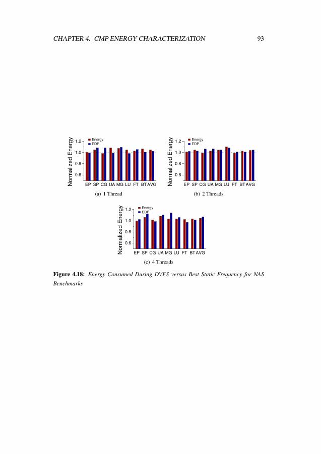
CHAPTER 4. CMP ENERGY CHARACTERIZATION 93
EP SP CG UA MG LU FT BTAVG
0.6
0.8
1.0
1.2
Norm
aliz
ed E
nerg
y
Energy
EDP
(a) 1 Thread
EP SP CG UA MG LU FT BTAVG
0.6
0.8
1.0
1.2
Norm
aliz
ed E
nerg
y
Energy
EDP
(b) 2 Threads
EP SP CG UA MG LU FT BTAVG
0.6
0.8
1.0
1.2
Norm
aliz
ed E
nerg
y
Energy
EDP
(c) 4 Threads
Figure 4.18: Energy Consumed During DVFS versus Best Static Frequency for NAS
Benchmarks

CHAPTER 4. CMP ENERGY CHARACTERIZATION 94
amm
p
applu
apsi
mgr
id
quak
e
swim
wup
wise
AVG
0.6
0.8
1.0
1.2N
orm
aliz
ed E
nerg
y
Energy
EDP
(a) 1 Thread
amm
p
applu
apsi
mgr
id
quak
e
swim
wup
wise
AVG
0.6
0.8
1.0
1.2
Norm
aliz
ed E
nerg
y
Energy
EDP
(b) 2 Threads
amm
p
applu
apsi
mgr
id
quak
e
swim
wup
wise
AVG
0.6
0.8
1.0
1.2
Norm
aliz
ed E
nerg
y
Energy
EDP
(c) 4 Threads
Figure 4.19: Energy Consumed During DVFS versus Best Static Frequency for SPEC
OMP2001 Benchmarks
asta
r
bwav
es
bzip2
cactus
ADM
calculix
dealII
gam
ess
gcc
G
emsF
DTD
gobm
k
grom
acs
h264
ref
hmm
erlbm
leslie3d
libqu
antu
mm
cfm
ilc
nam
d
omne
tpp
perlb
ench
povr
ay
sjen
g
soplex
xalanc
bmk
zeus
mp
Avera
ge
0.6
0.8
1.0
1.2
No
rma
lize
d E
ne
rgy
Energy
EDP
Figure 4.20: Energy Consumed during DVFS versus Best Static Frequency for SPEC
2006 benchmarks

CHAPTER 4. CMP ENERGY CHARACTERIZATION 95
• Serial fraction. Ideally, while executing the serial portion1 of the application(when only one core is doing useful work), the other cores should consume nopower. This can be achieved by power gating idle cores. But since a time penaltyis associated with bringing the power gated core back to an active state, the pro-cessor only activates that state if it is sure that the time penalty is worth it. De-pending on the length of serial portions, the processor may instead either let idlecores remain in active states or let them enter intermediate sleep states in whichthe core (or parts of it) may be clock gated but not power gated. Hence, the idlecores may consume some power, which directly contributes to the energy over-head of running applications in parallel.
• Core-to-core communication overhead. Most of the parallel threads share datato some extent. When one core requests data from another core, the executionpipeline of the first core may be stalled if its execution window does not haveenough independent instructions to hide the remote cache access latency. Thepower consumed in the core during these execution stalls adds to the energy over-head of parallelism.
• Bandwidth contention. Depending on the application, the working set may growwhen the number of parallel threads is increased. This could lead to increasedcontention for off-core and off-chip resources, resulting in potential increase inexecution stalls, which in turn adds to the energy overhead.
• Locking mechanism overhead. In lock-based applications, as the number of par-allel threads grows, the contention among threads trying to acquire the same lockalso increases. Depending on the lock mechanism employed, this could result inincreased execution cycles and/or total instructions executed, with both scenar-ios adding to the energy overhead. Another synchronization mechanism that canpotentially increase total instructions executed is hardware/software transactionalmemory, which will be covered in Chapter 5.
We use our power models to analyze how thread scaling under the influence of variationsin the listed parameters affects total energy energy expenditure and that of the core anduncore components.
To accurately study the affect of these parameters on the energy efficiency of threadscaling, we need must vary them in isolation. It is possible to do so using the same tech-nique we use for DVFS scaling: simulate a hypothetical microbenchmark by feedingappropriate values to the power model. However, this would require creating a thread-scaling performance model that takes into account variables like remote core access
1we user the term “serial portion” to refer to individual serial sections of the application and“serial fraction” to refer to the sum of all serial portions as fraction of total application
CHAPTER 4. CMP ENERGY CHARACTERIZATION 96
latency, locking mechanism overhead, and effects of bandwidth contention on perfor-mance. In addition to the inputs required for performance modeling, other parame-ters like temperature variations, sleep state latencies, and instruction count overheadsfrom synchronization primitives, make it more difficult to calculate a simulated applica-tion’s performance and energy accurately. To avoid these limitations, we instead use a(real) microbenchmark for thread-scaling analysis and measure performance from runson hardware instead of using performance model. We leverage the code from Eigen-bench [114] developed by Hong et al. to create microbenchmarks for characterizing theenergy when scaling numbers of threads. Eigenbench is a parameterized microbench-mark created to characterize the design space of transactional memory (TM) systemsby defining TM-related characteristics that can be explored orthogonally. The same ap-proach can be used to characterize the energy efficiency of thread scaling by definingorthogonal communication parameters and studying the effects of their variation on en-ergy expenditure during thread scaling.
In the following sections, we describe the energy characterization analysis of threadscaling when varying individual application characteristics. The core and uncore fre-quency is fixed at 3.4 GHz for all analyses in this section.
4.4.1 Energy Effects of Serial FractionTo analyze how the serial fraction of a parallel application affects its energy expenditure,we need a microbenchmark for which the serial fraction can be easily parameterized. Inthe original Eigenbench code, all work is done from the function eigenbench_core,which is called from within the parallel threads. To accurately control and vary theserial fraction of the application — without requiring to create a critical section — wecall eigenbench_core from both inside and outside the parallel section. We thenestimate the serial fraction of the application as the ratio of the total read and writeoperations done from the serial fraction to the sum of the reads and writes from bothserial and parallel sections. We verify the serial fraction thus calculated by comparing theexecution time predicted Equation: 4.19 (based on Amdahl’s Law) to actual executiontime. As per our experimental results, this gives us a reasonably accurate estimate of theapplication’s serial fraction. Figure 4.21 shows the pseudo-code for the microbenchmarkwe use in this analysis.
TN2 = TN1 ∗ (S + (1− S) ∗ N1
N2) (4.19)

CHAPTER 4. CMP ENERGY CHARACTERIZATION 97
Test oloop iloop array1 array2 R1 W1 R2 W2 Frequency Range
Serial-Large 100 10000 32KB 32KB 0 Var 0 Var 3.4 GHz W2 + W1 = 100, W2 = 0, 20, 40,...,100Serial-Small 100 300 32KB 32KB 0 Var 0 Var 3.4 GHz W2 + W1 = 100, W2 = 0, 20, 40,...,100
Table 4.4: Microbenchmark Parameters for Serial Fraction Analysis
where TNx = Execution time when number of parallel threads = x
S = Serial fraction of the application
During execution of the serial portion of the application, the idle cores (cores notrunning that serial portion) go into a sleep state (C-state on Intel machines). The biggerthe serial portion, the deeper the sleep state that the idle cores can enter, and the largerthe energy savings. The size of the serial portion depends on the number of operations inthe eigenbench_core function, which, in turn, depends on the value of the variableiloop. For our analysis, we test with two sizes of iloop: 10000, which make surethat the idle cores during the serial portion enter the deepest sleep state (C7), and 300,which does not give enough time for idle cores to enter a sleep state deeper than C3.Table 4.4 lists the parameters we use for testing the sensitivity of energy expenditure onan application’s serial fraction.
Figure 4.22 shows the energy expenditure and execution times from our analysis.Both the energy consumption and execution time values are normalized to those obtainedfor single-thread runs. We make the following observations about our results:
Observation 1: When the number of threads grows, the fraction of uncore energyto total chip energy goes down.
Explanation: This test does not share any data among parallel threads and theworking-set fits in L2 cache. Hence the number of uncore accesses are negligible. Thismeans that the uncore energy (both static and dynamic) is almost entirely idle energy.When only one core is active, this uncore idle energy constitutes 58% of total chip en-ergy at a 0% serial fraction. When parallelism is introduced and more cores are active,the ratio of uncore idle power to total chip power goes down, and as a result, we seea reduction in uncore static and dynamic energy with increasing numbers of threads.At a 0% serial fraction in Figure 4.22(a), the uncore idle energy fraction goes down to42% for two threads and 26% for four threads. When the serial fraction increases, thereduction in uncore idle energy becomes less pronounced. For example at 20% serialfraction in Figure 4.22(a), the serial fraction goes down from 58% at one thread to 46%at two threads and 35% at four threads. This is because when the application’s serialfraction increases, the performance gain from increasing the number of threads dimin-ishes. When the application is completely serial, there is no performance gain when the

CHAPTER 4. CMP ENERGY CHARACTERIZATION 98
void eigenbench_core(loop,r,w,array) {
long val = 0;
for (i=0; i<iloop; i++) {
for (j=0; j<(w+r) ; j++) {
(action) = rand_action(w, r);
index = rand_index(tid, array);
if (action == READ)
val += array[index];
elsearray[index] = val;
}
}
}
void main() {
int R1,W1,R2,W2; // R1 and W1: reads and writes in serial
// R2 and W2: reads and writes in parallel
long *array2[NUM_THREADS], *array1; //array1 is accessed
serially
//array2 is accessed by
parallel threads;
// but each thread writes
in own copy of array2
int iloop,oloop,array2_size,array1_size;
set_params(R1,W1,R2,W2,iloop,oloop,array1_size,array2_size);
Initialize_array(array1,array1_size);
for(j=0;j<NUM_THREADS;j++) {
Initialize_array(array2[j],array2_size);
}
for(i=0;i<oloop;i++) {
for(j=0;j<NUM_THREADS;j++) {
// ARGS -> iloop/NUM_THREADS, R2, W2, array2[j]
thread_start(eigenbench_core(),ARGS);
}
barrier();
eigenbench_core(iloop,R1,W1,array1);
}
}
Figure 4.21: Pseudo-Code for Serial Fraction Analysis

CHAPTER 4. CMP ENERGY CHARACTERIZATION 99
degree of parallelism increases. This is why there is no reduction in uncore idle energyfrom one to four threads. This analysis highlights the role of energy expenditure in theidle uncore.
Observation 2: The degree of parallelism at which the lowest energy is expendeddepends on the serial fraction and the size of the serial portion of the application.
Explanation: When the serial fraction is small, increasing the number of parallelthreads always results in reduced energy expenditures because of the reduction in uncoreidle energy discussed above. When the serial fraction increases, which results in lowerspeedups, we still see reductions in energy for applications with large serial portions.This is because when the serial portion is large, the inactive cores enter the C7 sleepstate in which the core is power gated, and hence they do not consume either static ordynamic power. As a result, core dynamic and static energy remain the same acrossvarying serial fraction and degrees of parallelism, as Figure 4.22(a) shows. Combinedwith reductions in uncore energy, this results in decreases in total chip energy (until theserial fraction hits 100%). But when the serial portion is small, the inactive cores onlyenter the shallower sleep states (C1/C1E/C3) in which the cores are not power gated andonly partially clock gated. The cores still consume static and dynamic power, resultingin increases in core static and dynamic energy as numbers of threads are increased. Thisoffsets the reduction in uncore energy to some extent. Figure 4.22(b) shows that at lowerserial fraction, the reduction in uncore energy offsets the increase in core energy at alldegrees of parallelism, and hence running the application at four threads is most energyefficient. At around a 40% serial fraction, when the number of threads increases fromtwo to four, the reduction in uncore energy is not enough to offset the increase in coreenergy, and hence energy expenditure at two threads is less than at four threads, eventhough the execution time at four threads is smaller. As the serial fraction is increased,this effect becomes more pronounced. When the serial fraction is greater 80% or more,it becomes more energy efficient to simply run the application serially.
4.4.2 Energy Effects of Core-to-core Communication Over-head
To analyze the effects of core-to-core communication on the energy efficiency of threadscaling, we need our microbenchmark to accurately control the fraction of shared mem-ory writes to total memory writes. We tweak the microbenchmark for serial fractionanalysis to use two buffers from the eigenbench_core function: one (array2) isprivate to the thread and hence does not generate coherence operations, and the other(array1) is shared among the threads and hence generates coherence operations. Fig-ure 4.23 shows the pseudocode for this analysis. In this version of the pseudocode, we

CHAPTER 4. CMP ENERGY CHARACTERIZATION 100
1 2 4 1 2 4 1 2 4 1 2 4 1 2 4 1 2 4
0
0.5
1.0
1.5
2.0N
orm
aliz
ed
En
erg
y (
Tim
e)
Uncore Dynamic EnergyUncore Static EnergyCore Dynamic EnergyCore Static EnergyExecution Time
0% 20% 40%
Serial Portion of Application
60% 80% 100%#threads
(a) Large serial portion: iloop=10000
1 2 4 1 2 4 1 2 4 1 2 4 1 2 4 1 2 4
0
0.5
1.0
1.5
2.0
No
rma
lize
d E
ne
rgy (
Tim
e)
Uncore Dynamic EnergyUncore Static EnergyCore Dynamic EnergyCore Static EnergyExecution Time
0% 20% 40%
Serial Portion of Application
60% 80% 100%#threads
(b) Small serial portion: iloop=300
Figure 4.22: Effects of Serial Fraction on the Energy Efficiency of Thread Scaling
Test iloop array1 array2 R1 W1 R2 W2 Frequency Range
Core-to-core 50000 32KB 32KB 0 Var 0 Var 3.4 GHz W2 + W1 = 100, W2 = 0, 20, 40,...,100
Table 4.5: Microbenchmark Parameters for Core-to-core Communication Overhead
Analysis
do not call the work function from outside the parallel section, and hence the serial frac-tion is always zero. We do not use synchronization primitives to protect shared writesbecause we only want to isolate the effects of core-to-core communication overheadsand correctness is not of essence here.
Table 4.5 lists the parameters used for testing sensitivity of energy expenditure oncore-to-core communication overhead. Figure 4.24 shows the execution time and en-ergy expenditure trends for varying fractions of shared writes to total writes by parallelthreads. Both energy and execution times are normalized to those for single-thread runs.The absolute energy expenditure at all single-thread runs is the same, since for single-thread runs all cache access hit in the private L1/L2 caches.
We make the following observations from these results.Observation 1: The execution time and energy expenditure are almost the same for
0% and 20% shared writes, even though there is a significant increase in L2 misses forthe latter.
Explanation: When only 20% of the memory accesses are shared, the latency ofgetting data from a remote cache is hidden by the instruction-level parallelism in the

CHAPTER 4. CMP ENERGY CHARACTERIZATION 101
void eigenbench_core(loop,r1,w1,array1,r2,w2,array2) {
long val = 0;
for (i=0; i<iloop; i++) {
for (j=0; j<(w1+r1+w2+r2) ; j++) {
(action) = rand_action(r1, w1, r2, w2);
index = calc_index(tid, array); //Randomization not used to
//avoid non-buffer memory
ops
if (action == READ1)
val += array1[index];
else if (action == WRITE1)
array1[index] = val;
else if (action == READ2)
val += array2[index];
elsearray2[index] = val;
}
}
}
void main() {
int R1,W1,R2,W2; // R1 and W1: reads and writes in array1
// R2 and W2: reads and writes in array2
long *array2[NUM_THREADS], *array1; // Each thread writes in
own copy of array2
// array1 is shared among
parallel threads
int iloop,oloop,array2_size,array1_size;
set_params(R1,W1,R2,W2,iloop,oloop,array1_size,array2_size);
Initialize_array(array1,array1_size);
for(j=0;j<NUM_THREADS;j++) {
Initialize_array(array2[j],array2_size);
}
for(j=0;j<NUM_THREADS;j++) {
// ARGS -> iloop/NUM_THREADS, R1, W1, array1, R2, W2, array2[
j]
thread_start(eigenbench_core(),ARGS);
}
}
Figure 4.23: Pseudo-Code for Core-to-core Communication Overhead Analysis
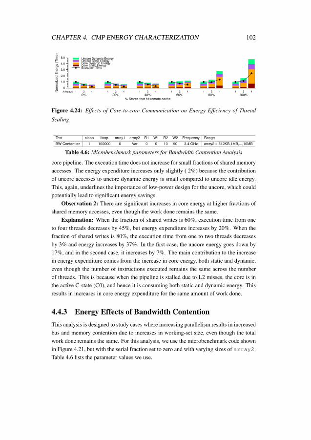
CHAPTER 4. CMP ENERGY CHARACTERIZATION 102
1 2 4 1 2 4 1 2 4 1 2 4 1 2 4 1 2 4
0
1.0
2.0
3.0
4.0
5.0N
orm
aliz
ed
En
erg
y (
Tim
e)
Uncore Dynamic EnergyUncore Static EnergyCore Dynamic EnergyCore Static EnergyExecution Time
0% 20% 40%
% Stores that hit remote cache
60% 80% 100%#threads
Figure 4.24: Effects of Core-to-core Communication on Energy Efficiency of Thread
Scaling
Test oloop iloop array1 array2 R1 W1 R2 W2 Frequency Range
BW Contention 1 100000 0 Var 0 0 10 90 3.4 GHz array2 = 512KB,1MB,...,16MB
Table 4.6: Microbenchmark parameters for Bandwidth Contention Analysis
core pipeline. The execution time does not increase for small fractions of shared memoryaccesses. The energy expenditure increases only slightly ( 2%) because the contributionof uncore accesses to uncore dynamic energy is small compared to uncore idle energy.This, again, underlines the importance of low-power design for the uncore, which couldpotentially lead to significant energy savings.
Observation 2: There are significant increases in core energy at higher fractions ofshared memory accesses, even though the work done remains the same.
Explanation: When the fraction of shared writes is 60%, execution time from oneto four threads decreases by 45%, but energy expenditure increases by 20%. When thefraction of shared writes is 80%, the execution time from one to two threads decreasesby 3% and energy increases by 37%. In the first case, the uncore energy goes down by17%, and in the second case, it increases by 7%. The main contribution to the increasein energy expenditure comes from the increase in core energy, both static and dynamic,even though the number of instructions executed remains the same across the numberof threads. This is because when the pipeline is stalled due to L2 misses, the core is inthe active C-state (C0), and hence it is consuming both static and dynamic energy. Thisresults in increases in core energy expenditure for the same amount of work done.
4.4.3 Energy Effects of Bandwidth ContentionThis analysis is designed to study cases where increasing parallelism results in increasedbus and memory contention due to increases in working-set size, even though the totalwork done remains the same. For this analysis, we use the microbenchmark code shownin Figure 4.21, but with the serial fraction set to zero and with varying sizes of array2.Table 4.6 lists the parameter values we use.

CHAPTER 4. CMP ENERGY CHARACTERIZATION 103
1 2 4 1 2 4 1 2 4 1 2 4 1 2 4 1 2 4
0
0.5
1.0
1.5
2.0N
orm
aliz
ed
En
erg
y (
Tim
e)
Uncore Dynamic EnergyUncore Static EnergyCore Dynamic EnergyCore Static EnergyExecution Time
512K 1M 2M
Working-set size per thread
4M 8M 16M#threads
Figure 4.25: Effects of Bandwidth Contention on Energy Efficiency of Thread Scaling
The execution time and energy expenditure results from this analysis are shown inFigure 4.25. The working-set size on the x-axis is per thread. We make the followingobservations from these results.
Observation 1: There is almost no time or energy penalty for increases in contentionwhen the total working-set size fits within L3 cache.
Explanation: When the working-set size per thread is less than 2 MB, the workingset fits in the 8 MB L3 cache at all levels of parallelism. When the working set perthread is increased from 512KB to 1MB, we see an increase of around 17% in totalL2 misses, but no increase in execution time or energy. Even when we decrease theworking-set size per thread to 128 KB (not shown in the figure), the execution time andenergy do not change significantly, even though the number of L2 misses does decreaseas expected. This is because the latency of fetching data from the L3 is short enough thatinstruction level parallelism in pipeline can hide it. The energy also remains the samebecause, again, the energy expenditure due to L2 misses is a small fraction of uncoreidle energy.
Observation 2: When the total working-set size does not fit in the L3 cache, run-ning at two threads expends the least energy, even though four threads gives the lowestexecution time.
Explanation: As we observed in the core-to-core communication analysis, whencore execution is stalled due to data dependencies on L3 misses, the core waits for datain an active state, and hence it consumes static and dynamic energy. Also, as we observedbefore, any speedup due to parallelism almost always leads to reduction in uncore en-ergy. When the parallelism leads to increased memory contention but still delivers somespeedup, uncore energy is reduced, but core energy is increased due to stall cycles. Go-ing from one to two threads, the reduction in uncore energy is greater than the increasein core energy. However, going from two to four threads, the increase in core energyoffsets the reduction in uncore energy, resulting in the energy trends we observe in ourresults.

CHAPTER 4. CMP ENERGY CHARACTERIZATION 104
Test iloop array R1 W1 R2 W2 Frequency Range
Lock Overhead 100000 32KB 0 Var 0 Var 3.4 GHzW1=100,50,40,30,20,10
W2=W1*9
Table 4.7: Microbenchmark Parameters for Lock-Overhead Analysis
4.4.4 Energy Effects of Locking-Mechanism OverheadIn this analysis, we characterize the effects of overheads related to locking mechanismson the energy efficiency of thread scaling. Figure 4.26 shows the pseudo-code of themicrobenchmark we use for this test. We use a pthreads mutex as the locking mecha-nism. Table 4.7 shows the parameter values we use. We vary the size of critical sectionby controlling the number of stores inside it. The number of stores outside the criticalsection is always equal to nine times the number from inside (W2 = W1 × 9), whicheffectively sets the serial fraction of the application to 10%. We observe the effects oflocking-mechanism overhead on the energy efficiency of thread scaling as we decreasethe size of the critical section. Figure 4.27 shows our results.
We make following observations from these results.Observation 1: The core energy increases significantly with increases in the num-
ber of parallel threads. When the critical section is large (100 stores), the core energyincreases by 16% from one to two threads and by 40% from one to four threads. Whenthe critical section is small (10 stores), the core energy increases by 93% from one totwo threads and 133% from one to four threads.
Explanation: As we saw in our serial fraction analysis for the case where the serialportion of the application is small (Figure 4.22(b)), core energy is expected to increasewhen parallelism is introduced due to inactive cores not being able to enter deeper sleepstates. In this case, the critical section is small enough that the inactive cores spend theiridle cycles in either the active state or the shallowest sleep state (C1/C1E), resultingin increase sin energy consumption. Moreover, as the critical section gets smaller, theoverhead of acquiring and releasing locks gets higher. When the critical section has 100stores, the total instruction execution count increases by 3% from one to four threads.When the critical section has only 10 stores, the instruction count increases by 15% fromone to four threads, contributing to the overall increase in core energy expenditure.
Observation 2: For small critical sections, the energy expenditure at two threads ismore than the energy expenditure at one and four threads. Also, running at one thread ismost energy efficient, even when running at four threads gives best performance.
Explanation: When the size of the critical section is reduced, the overhead relatedto acquiring the lock starts affecting both speedup and the energy efficiency of threadscaling. When the application is scaled from one to two threads, the energy reductionin the uncore (due to speedup) is not enough to offset the energy increase. When the

CHAPTER 4. CMP ENERGY CHARACTERIZATION 105
void eigenbench_core(loop,r1,w1,r2,w2,array) {
long val = 0;
for (i=0; i<iloop; i++) {
acquire_lock();
for (j=0; j<(w1+r1) ; j++) {
(action) = rand_action(w1, r1);
index = rand_index(tid, array);
if (action == READ)
val += array[index];
elsearray[index] = val;
}
release_lock();
barrier();
for (j=0; j<(w2+r2) ; j++) {
(action) = rand_action(w2, r2);
index = rand_index(tid, array);
if (action == READ)
val += array[index];
elsearray[index] = val;
}
}
}
void main() {
int R1,W1,R2,W2; // R1 and W1: reads and writes inside critical
section
// R2 and W2: reads and writes outside
critical section
long *array[NUM_THREADS]; //array is accessed by parallel
threads;
// but each thread writes in own copy
of array
int iloop,array_size;
set_params(R1,W1,R2,W2,iloop,array_size);
for(j=0;j<NUM_THREADS;j++) {
Initialize_array(array[j],array_size);
}
for(j=0;j<NUM_THREADS;j++) {
// ARGS -> iloop/NUM_THREADS, R1, W1, R2, W2, array[j]
thread_start(eigenbench_core(),ARGS);
}
}
Figure 4.26: Pseudo-Code for Locking Mechanism Overhead Analysis

CHAPTER 4. CMP ENERGY CHARACTERIZATION 106
1 2 4 1 2 4 1 2 4 1 2 4 1 2 4 1 2 4
0
0.5
1.0
1.5
2.0N
orm
aliz
ed
En
erg
y (
Tim
e)
Uncore Dynamic EnergyUncore Static EnergyCore Dynamic EnergyCore Static EnergyExecution Time
100 50 40
No. of stores in critical section
30 20 10#threads
Figure 4.27: Effects of Locking-Mechanism Overhead on the Energy Efficiency of
Thread Scaling
application is scaled from two to four threads, the speedup obtained further reducesuncore energy expenditure, which this time offsets the increase in core energy but notenough to reduce the energy expenditure compared to the run at a single thread. We seethis trend for all sizes of critical sections smaller than or equal to 20 stores. But thisholds true only when the serial fraction is small enough that increasing the number ofthreads provides significant speedups. If the serial fraction is increased from 10% togreater than 60%, the speedup obtained going from two to four threads is not enoughto offset the increase in core energy expenditure, and, as a result, total energy at fourthreads is higher than the energy value at two threads.
4.5 Related WorkVarious publications in the past have explored the usage of performance counters forpower estimation. Some of the related work has already been discussed in the previouschapter. Here, we discuss previous research on power estimation modeling that explicitlyattempts to differentiate between static and dynamic power consumption.
The power model proposed by Bertran et al. [50] makes a distinction between dy-namic and static power. However, they define static power as idle power and use regres-sion on the values of their chosen events to derive both static (idle) and dynamic power.Unlike us, their power models disregard both voltage and temperature and hence, cannotbe used for characterizing the true static and dynamic power consumption of the chip.
Spiliopoulos et al. [36] also address static and dynamic power separately in theirapproach to power estimation, but they also define static power as idle power. Theycreate a table (offline) of idle power values at all frequency steps and “typical core tem-perature ranges”. We instead differentiate between static power (based on voltage andtemperature) and idle dynamic power.
Huang et al. [117] present the methdology used to develop a power proxy for esti-mating per-core power consumption for IBM POWER7+ server chip. They break down

CHAPTER 4. CMP ENERGY CHARACTERIZATION 107
the power consumption values in active power, clock grid power and leakage power.They leverage the in-house information available about the technology constants to buildtheir power model while our methodology requires no such prior knowledge. Theirpower estimation logic is implemented partly in hardware and partly in firmware andhence, requires on-chip hardware support; while our model is implemented fully in soft-ware.
Su et al. [109] use 12 performance events to estimate power consumption for theirAMD system and hence, require time-multiplexing to gather data for all events. Theyaddress idle and dynamic power separately. Like our second approach, they use voltageand temperature to develop a static power model, but they group idle dynamic powerinto their static power model, which does not reflect the true static power consumptionof the core and the northbridge (equivalent to the uncore in our models).
The use of power models to drive DVFS policies has also been explored by some ofthe previous research papers.
Su et al. [109] and Spiliopoulos et al. [36] use their performance and energy es-timation models to predict the voltage-frequency operating point at which the currentapplication phase will expend lowest energy/EDP. In contrast to our work, their DVFSscheduler needs to perform energy calculations for each available DVFS operating pointat runtime, while we use a look-up table to directly predict the low energy/EDP op-erating point without the need to perform any calculations and hence, induces loweroverhead. This makes our methodology more suitable for future systems where schedul-ing decisions need to be taken more frequently and possibly, across more number ofvoltage-frequency pairs.
Su et al. [109] also their models to characterize energy expenditure on their AMDFX-8320 system at various frequencies. Their system always expends least energy atthe lowest voltage-frequency state in contrast to our observations on Haswell machine.The frequency scaling energy trends would differ among microarchitectures and imple-mentations depending on the energy expenditure fraction of idle uncore (or Northbridge)which is affected by the level of clock and power gating.
Patki et al. [112] develop a power-aware job scheduler for power constrained cluster.Like our DVFS scheduler, their scheduling policies also rely upon a look-up table popu-lated with details like execution time and power for certain application configurations inadvance to achieve the scheduling complexity of O(1).
Dzhagaryan et al. [118] study the impact of thread and frequency scaling on perfor-mance and energy expenditure of Intel Xeon processor. Unlike us they do not analyze theunderlying reasons for the observed energy trends, namely the static and dynamic powerconsumption of core and uncore. They use PARSEC benchmarks for their study whilewe use microbenchmarks to isolate the effect of individual communication parameters.
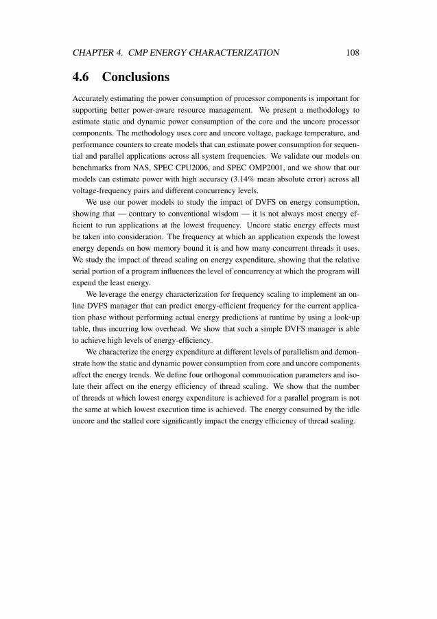
CHAPTER 4. CMP ENERGY CHARACTERIZATION 108
4.6 ConclusionsAccurately estimating the power consumption of processor components is important forsupporting better power-aware resource management. We present a methodology toestimate static and dynamic power consumption of the core and the uncore processorcomponents. The methodology uses core and uncore voltage, package temperature, andperformance counters to create models that can estimate power consumption for sequen-tial and parallel applications across all system frequencies. We validate our models onbenchmarks from NAS, SPEC CPU2006, and SPEC OMP2001, and we show that ourmodels can estimate power with high accuracy (3.14% mean absolute error) across allvoltage-frequency pairs and different concurrency levels.
We use our power models to study the impact of DVFS on energy consumption,showing that — contrary to conventional wisdom — it is not always most energy ef-ficient to run applications at the lowest frequency. Uncore static energy effects mustbe taken into consideration. The frequency at which an application expends the lowestenergy depends on how memory bound it is and how many concurrent threads it uses.We study the impact of thread scaling on energy expenditure, showing that the relativeserial portion of a program influences the level of concurrency at which the program willexpend the least energy.
We leverage the energy characterization for frequency scaling to implement an on-line DVFS manager that can predict energy-efficient frequency for the current applica-tion phase without performing actual energy predictions at runtime by using a look-uptable, thus incurring low overhead. We show that such a simple DVFS manager is ableto achieve high levels of energy-efficiency.
We characterize the energy expenditure at different levels of parallelism and demon-strate how the static and dynamic power consumption from core and uncore componentsaffect the energy trends. We define four orthogonal communication parameters and iso-late their affect on the energy efficiency of thread scaling. We show that the numberof threads at which lowest energy expenditure is achieved for a parallel program is notthe same at which lowest execution time is achieved. The energy consumed by the idleuncore and the stalled core significantly impact the energy efficiency of thread scaling.

5Characterization of Intel’s Restricted
Transactional Memory
Transactional memory (TM) [119] simplifies some of the challenges of shared-memoryprogramming. The responsibility for maintaining mutual exclusion over arbitrary sets ofshared-memory locations is devolved to the TM system, which may be implemented insoftware (STM) or hardware (HTM). TM presents the programmer with fairly easy-to-use programming constructs that define a transaction — a piece of code whose executionis guaranteed to appear as if it occurred atomically and in isolation.
The research community has explored this design space in depth, and a variety ofproposed systems take advantage of transaction characteristics to simplify implementa-tion and improve performance [120–123]. Hardware support for transactional memoryhas been implemented in Rock [124] from Sun Microsystems, Vega from Azul Sys-tems [125], and Blue Gene/Q [126] and System z [127] from IBM. Haswell is the first In-tel product to provide such hardware support. Intel’s Transactional Synchronization Ex-tensions (TSX) allow programmers to run transactions on a best-effort HTM implemen-tation, i.e., the platform provides no guarantees that hardware transactions will commitsuccessfully, and thus the programmer must provide a non-transactional path as a fall-
109

CHAPTER 5. CHARACTERIZATION OF INTEL’S RTM 110
back mechanism. Intel TSX supports two software interfaces to execute atomic blocks:Hardware Lock Elision (HLE) is an instruction set extension to run atomic blocks onlegacy hardware, and Restricted Transactional Memory (RTM) is a new instruction setinterface to execute transactions on the underlying TSX hardware.
The previous chapters have highlighted the need for better hardware introspectioninto power consumption. As better hardware support for such introspection becomesavailable, it is important to evaluate accuracy and acuity so that users can choose amongvarious combinations of measurement and modeling techniques. Since Intel’s Core i74770 microarchitecture is among the first to support both power modeling and supportfor transactional memory, it makes an interesting platform for analyzing power/perfor-mance trade-offs.
As an initial study, we compare the Haswell RTM performance and energy of theHaswell implementation of RTM to those of other approaches for controlling concur-rency. We use a variety of workloads to test the susceptibility of RTM’s best-effort natureto performance degradation and increased energy consumption. We compare RTM per-formance to TinySTM, a software transactional memory implementation that uses timeto reason about the consistency of transactional data and about the order of transactioncommits.1 We highlight these crossover points and analyze the impact of thread scalingon energy expenditure.
We find that RTM performs well with small to medium working sets when theamount of data (particularly that being written) accessed in transactions is small. Whendata contention among concurrent transactions is low, TinySTM performs better thanRTM, but as contention increases, RTM consistently wins. RTM generally suffers lessoverhead than TinySTM for single-threaded runs, and it is more energy-efficient whenworking sets fit in cache.
5.1 Experimental SetupThe Intel 4th Generation CoreTM i7 4770 processor comprises four physical cores thatcan run up to eight simultaneous threads when hyper-threading is enabled. Each corehas two eight-way 32 KB private L1 caches (separate for I and D), a 256 KB private L2cache (for combined I and D), and an 8 MB shared L3 cache, with 16 GB of physicalmemory on board. We compile all microbenchmarks, benchmarks, and synchronizationlibraries using gcc v4.8.1 with -O3 optimization flag. We use the -mrtm flag to accessthe Intel TSX intrinsics. We schedule threads on separate physical cores (unless runningmore than four threads) and fix the CPU affinity to prevent migration.
1We choose TinySTM because during our experiments we find that it consistently outperformsother STM alternatives like TL2 (to which RTM was compared in another recent study [128]).

CHAPTER 5. CHARACTERIZATION OF INTEL’S RTM 111
We modify the task example from libpfm4.4 to read both the performance countersand the processor package energy via the Running Average Power Limit (RAPL) [84]interface. As we concluded in Chapter 2, RAPL is fairly accurate when the time be-tween successive RAPL counter reads is more than tens of milliseconds. Since all ourbenchmarks run for at least few seconds, we decided to use RAPL for our energy mea-surements. We implement Intel TSX synchronization as a separate library and add RTMdefinitions to the STAMP tm.h file. When transactions fail more than eight times, weinvoke reader/writer lock-based fallback code to ensure forward progress. If the returnstatus bits indicate that an abort was due to another thread’s having acquired the lock (inthe fallback code), we wait for the lock to be free before retrying the transaction. Thefollowing shows pseudocode for a sample transaction.
Algorithm 1 Implementation of BeginTransaction
while true donretries← nretries + 1status← _xbegin()if status = _XBEGIN_STARTED then
if arch_read_can_lock(serialLock) thenreturn
else_xabort(0)
end ifend if{*** fall-back path ***}while not arch_read_can_lock(serialLock) do
_mmpause()end whileif nretries ≥MAX_RETRIES then
breakend if
end whilearch_write_lock(serialLock);return

CHAPTER 5. CHARACTERIZATION OF INTEL’S RTM 112
1 2 4 8 16 32 6412825
651
2 1K 2K 4K 8K16K32
K64
K12
8K
Transaction Size (Cache Blocks)
0
20
40
60
80
100
A
bort
Rate
(%
)
read-set aborts
write-set aborts
Figure 5.1: RTM Read-Set and Write-Set Capacity Test
5.2 Microbenchmark analysis
5.2.1 Basic RTM EvaluationWe first quantify RTM’s hardware limitations that affect its performance using mi-crobenchmark studies. We detail the results of these experiments below.
RTM Capacity Test. To test the limitations of read-set and write-set capacity forRTM, we create a custom microbenchmark, results for which are shown in Fig. 5.1. Theabort rate of write-only transactions tops out at 512 cache blocks (the size of L1 datacache). We suspect this is because write-sets are tracked only in L1, and so evicting anytransactionally written cache line from L1 results in a transaction abort. For read-sets,the abort rate saturates at 128K cache blocks (the size of L3 cache). This suggests thatevicting transactionally read cache lines from L3 (but not L1) triggers transaction aborts,and thus RTM maintains performance for much larger read-sets than write-sets.
RTM Duration Test. Since RTM aborts can be caused by system events like in-terrupts and context switches, we study the effects of transaction duration (measured inCPU cycles) on success rate. For this analysis, we use a single thread, set the working-set size to 64 bytes, and set the number of writes inside the transaction to 0. This tries toensure that the number of aborts due to memory events and conflicts remains insignifi-cant. We gradually increase the duration by increasing the number of reads within thetransaction. Fig. 5.2 shows that transaction duration begins to affect the abort rate atabout 30K cycles and that durations of more than 10M cause all transactions to abort(note that these results are likely machine dependent).
RTM Overhead Test. Next we quantify performance overheads for RTM comparedto spin locks and the atomic compare-and-swap (CAS) instruction. For this test, we cre-ate a microbenchmark that removes elements from a queue (defined in the STAMP [129]library). We initialize the queue to 1M elements, and threads extract elements until thequeue is empty. Work is not statically divided among threads. We first compare RTMagainst the spinlock implementation in the Linux kernel (arch/x86/include/asm/

CHAPTER 5. CHARACTERIZATION OF INTEL’S RTM 113
1K 10K 100K 1M 10M
Transaction Duration (CPU Cycles)
0
20
40
60
80
100
Ab
ort
Ra
te (
%)
Figure 5.2: RTM Abort Rate versus Transaction Duration
spinlock.h). We then compare against a version of the queue implementation modi-fied to use CAS in queue_pop(). For RTM, we simply retry the transaction on aborts.
We perform three sets of experiments. To observe the cost of starting an RTM trans-action in the absence of contention, we first run single-threaded experiments. We repeatthe experiment with four threads to generate a high-contention workload. Finally, welower contention by making threads work on local data for a fixed number of operationsafter each critical section. Table 5.1 summarizes execution times normalized to those ofthe lock-based version.
Type of synchronizationContention None Lock CAS RTMNone 0.64 1 1.05 1.45Low N/A 1 0.64 0.69High N/A 1 0.64 0.47
Table 5.1: Relative Overhead of RTM versus Locks and CAS
Table 5.1 shows that the cost of starting a transaction makes RTM perform worsethan the other alternatives when executing non-contended critical sections with few in-structions. RTM suffers about a 45% slowdown compared to using locks and CAS, andit takes over twice the time of an unsynchronized version. In contrast, our multi-threadedexperiments reveal that RTM exhibits roughly 30% and 50% lower overhead than locksin low and high contention, respectively, while CAS is in both cases around 35% bet-ter than locks. Note that transactions avoid hold-and-wait behavior, which seems togive RTM an advantage in our study. When comparing locks and CAS, the higher lockoverhead is likely due in part to the ping-pong coherence behavior of the cache linecontaining the lock and to cache-to-cache transfers of the line holding the queue head.

CHAPTER 5. CHARACTERIZATION OF INTEL’S RTM 114
Characteristic Definition
Concurrency Number of concurrently running threadsWorking-set sizea Size of frequently used memoryTransaction length Number of memory accesses per transactionPollution Fraction of writes to total memory accesses
inside transactionTemporal locality Probability of repeated address inside transactionContention Probability of transaction conflictPredominance Fraction of transactional cycles to total application
cycles
aWorking-set size for Eigenbench is defined per-thread.
Table 5.2: Eigenbench TM Characteristics
5.2.2 Eigenbench CharacterizationTo compare RTM and STM in detail, we next study the behaviors of Hong et al.’s Eigen-bench [114]. This parameterizable microbenchmark attempts to characterize the designspace of TM systems by orthogonally exploring different transactional application be-haviors. Table 5.2 defines the seven characteristics we use to compare performance andenergy expenditure of the Haswell RTM implementation and the TinySTM [130] soft-ware transactional memory system. Hong et al. [114] provide a detailed explanation ofthese characteristics and the equations used to quantify them.
Unless otherwise specified, we use the following parameters in our experiments,results for which we average over 10 runs. Transactions are 100 memory references (90reads and 10 writes) in length. We use one small (16KB) and one medium (256KB)working set size to demonstrate the differences in RTM performance. Since L1 size hasno influence on TinySTM’s abort rates, we only show TinySTM results for the smallerworking set size. To prevent L1 cache interference, we run four threads with hyper-threading disabled as our default, and we fix the CPU affinity to prevent thread migration.For each characteristic, we compare RTM and TinySTM performance and energy (versussequential runs of the same code) and transaction-abort rates. For the graphs in whichwe plot two working-set sizes for RTM, the speedups and energy efficiency given arerelative to the sequential run of the same size working set.
Working-Set Size. Fig. 5.3 shows Eigenbench results over a logarithmic scale aswe increase each thread’s working set from 8KB to 128MB. RTM performs best withthe smallest working set, and its performance gradually degrades as working-set size in-creases. The performance of both RTM and TinySTM drops once the combined workingsets of all threads exceed the 8MB L3 cache. RTM performance suffers more becauseevents like L3 evictions, page faults, and interrupts trigger a transaction abort, which

CHAPTER 5. CHARACTERIZATION OF INTEL’S RTM 115
10 100 1000 10000 100000
Working Set (KB/Thread)
0
1
2
3
4
Speedup (
4 T
hre
ads) RTM
TinySTM
(a) Speedup
10 100 1000 10000 100000
Working Set (KB/Thread)
0
1
2
Energ
y/E
nerg
y-S
equential
RTM
TinySTM
(b) Relative Energy
10 100 1000 10000 100000
Working Set (KB/Thread)
0
20
40
60
80
100
Ab
ort
Ra
te (
%)
RTM
TinySTM
(c) Abort Rate
Figure 5.3: Eigenbench Working-Set Size
is not the case for TinySTM. The speedups of both RTM and TinySTM are lowest atworking sets of 4MB: at this point, the parallelized code’s working sets (16MB in total)exceed L3, but the working set of the sequential version (4MB) still fits. For working setsabove 4MB, the sequential version starts encountering L3 misses, and thus the relativeperformances of both transactional memory implementations begins to improve. Par-allelizing the transactional code using RTM is energy-efficient compared to sequentialversion when the combined working sets of all threads fits inside the cache.
Transaction Length. Fig. 5.4 shows Eigenbench results as we increase the trans-action length from 10 to 520 memory operations. When the working set (16KB) fitswithin L1, RTM outperforms TinySTM for all transaction lengths. For 256KB workingsets, RTM performance drops sharply when the transaction length exceeds 100 accesses.Recall that evicting write-set data from the L1 triggers transaction aborts, but when theworking set fits within L1, such evictions are few. As the working set grows, the ran-domly chosen addresses accessed inside the transactions have a higher probability ofoccupying more L1 cache blocks, and hence they are more likely to be evicted. In con-trast, TinySTM shows no performance dependence on working-set size. The overhead ofstarting the hardware transaction affects RTM performance for very small transactions.As observed in the working-set analysis above, RTM is more energy efficient than boththe sequential run and TinySTM for all transaction lengths when using the smaller work-

CHAPTER 5. CHARACTERIZATION OF INTEL’S RTM 116
100 200 300 400 500
Transaction Length (Memory Operations)
0
1
2
3
4
Sp
ee
du
p (
4 T
hre
ad
s)
RTM 16K
RTM 256K
TinySTM
(a) Speedup
100 200 300 400 500
Transaction Length (Memory Operations)
0
1
2
3
En
erg
y/E
ne
rgy-S
eq
ue
ntia
l
RTM 16K
RTM 256K
TinySTM
(b) Relative Energy
100 200 300 400 500
Transaction Length (Memory Operations)
0
20
40
60
80
100
Ab
ort
Ra
te (
%)
RTM 16K
RTM 256K
TinySTM
(c) Abort Rate
Figure 5.4: Eigenbench Transaction Length
ing set. When using the larger working set, RTM expends more energy for transactionsexceeding 120 accesses.
Pollution. Fig. 5.5 shows results when we test symmetry (with respect to handlingread-sets and write-sets) by gradually increasing the fraction of writes. The pollutionlevel is zero when all memory operations in the transaction are reads and one when allare writes. When the working set fits within L1, RTM shows almost no asymmetry. Butfor the larger working-set size, RTM speedup suffers as the level of pollution increases.TinySTM outperforms RTM when the pollution level increases beyond 0.4.
Temporal Locality. We next study the effects of temporal locality on TM perfor-mance (where temporal locality is defined as the probability of repeatedly accessing thesame memory address within a transaction). The results in Fig. 5.6 reveal that RTMshows no dependence on temporal locality for the 16KB working set, but performancedegrades for the 256KB working set (where low temporal locality increases the numberof aborts due to L1 write-set evictions). In contrast, TinySTM performance degradesas temporal locality increases, indicating that it favors unique addresses unless only oneaddress is being accessed inside the transaction (locality = 1.0).
Contention. This analysis studies the behavior of TM systems when the level ofcontention is varied from low to high. We set the working-set size to 2MB for bothRTM and TinySTM. The level of contention is calculated as an approximate value rep-

CHAPTER 5. CHARACTERIZATION OF INTEL’S RTM 117
0.0 0.2 0.4 0.6 0.8 1.0
Pollution Ratio
0
1
2
3
4
Sp
ee
du
p (
4 T
hre
ad
s)
RTM 16K
RTM 256K
TinySTM
(a) Speedup
0.0 0.2 0.4 0.6 0.8 1.0
Pollution Ratio
0.0
0.5
1.0
1.5
En
erg
y/E
ne
rgy-S
eq
ue
ntia
l
RTM 16K
RTM 256K
TinySTM
(b) Relative Energy
0.0 0.2 0.4 0.6 0.8 1.0
Pollution Ratio
0
20
40
60
80
100
Ab
ort
Ra
te (
%)
RTM 16K
RTM 256K
TinySTM
(c) Abort Rate
Figure 5.5: Eigenbench Pollution
0.0 0.2 0.4 0.6 0.8 1.0
Temporal Locality
0
1
2
3
4
Sp
ee
du
p (
4 T
hre
ad
s)
RTM 16K
RTM 256K
TinySTM
(a) Speedup
0.0 0.2 0.4 0.6 0.8 1.0
Temporal Locality
0.0
0.5
1.0
En
erg
y/E
ne
rgy-S
eq
ue
ntia
l
RTM 16K
RTM 256K
TinySTM
(b) Relative Energy
0.0 0.2 0.4 0.6 0.8 1.0
Temporal Locality
0
20
40
60
80
100
Ab
ort
Ra
te (
%)
RTM 16K
RTM 256K
TinySTM
(c) Abort Rate
Figure 5.6: Eigenbench Temporal Locality

CHAPTER 5. CHARACTERIZATION OF INTEL’S RTM 118
0.0 0.2 0.4 0.6 0.8 1.0
Conflict Probability
0
1
2
3
4
Sp
ee
du
p (
4 T
hre
ad
s) RTM
TinySTM
(a) Speedup
0.0 0.2 0.4 0.6 0.8 1.0
Conflict Probability
0
2
4
6
En
erg
y/E
ne
rgy-S
eq
ue
ntia
l
RTM
TinySTM
(b) Relative Energy
0.0 0.2 0.4 0.6 0.8 1.0
Conflict Probability
0
20
40
60
80
100
Ab
ort
Ra
te (
%)
RTM
TinySTM
(c) Abort Rate
Figure 5.7: Eigenbench Contention
resenting the probability of a transaction causing a conflict (as per the probability for-mula given by Hong et al. [114]). The conflict probability figures shown in Fig. 5.7are calculated at word granularity and hence are specific to TinySTM. Since RTM de-tects conflicts at the granularity of cache line (64 bytes), the contention level is actuallyhigher for RTM with the same workload configuration. When the degree of contentionamong competing threads is very low, RTM performs better than TinySTM. For low tomedium contention, TinySTM considerably outperforms RTM. However, for high con-tention workloads, TinySTM performance degrades while RTM performance remainsalmost the same.
Predominance. We study the behavior of the TM systems when varying the frac-tion of application cycles executed within transactions to the total number of applicationcycles. For this analysis, we set working-set size to 256KB for both TM systems, we setcontention to zero, and we vary the predominance ratio from 0.125 to 0.875. Fig. 5.8shows that performance for both RTM and TinySTM suffers as the ratio of transactionalcycles to non-transactional cycles grows. This can be attributed to the overheads asso-ciated with the TM systems: for the same level of predominance, TinySTM introducesmore overhead because it must instrument the program memory accesses.
Concurrency. Next we study how the performance and energy of RTM and TinySTMscale when concurrency is increased from one thread to eight. Fig. 5.9 shows that RTM

CHAPTER 5. CHARACTERIZATION OF INTEL’S RTM 119
0.0 0.2 0.4 0.6 0.8 1.0
Predominance Rate
0
1
2
3
4
Sp
ee
du
p (
4 T
hre
ad
s)
RTM
TinySTM
(a) Speedup
0.0 0.2 0.4 0.6 0.8 1.0
Predominance Rate
0.0
0.5
1.0
En
erg
y/E
ne
rgy-S
eq
ue
ntia
l
RTM
TinySTM
(b) Relative Energy
0.0 0.2 0.4 0.6 0.8 1.0
Predominance Rate
0
20
40
60
80
100
Ab
ort
Ra
te (
%)
RTM
TinySTM
(c) Abort Rate
Figure 5.8: Eigenbench Predominance
scales well up to four threads. At eight threads, the L1 cache is shared between twothreads running on the same core. This cache sharing degrades performance for thelarger working set more than for the smaller working set because hyper-threading effec-tively halves the write-set capacity of RTM. In contrast, TinySTM scales well up to eightthreads. For the small working set, RTM proves to be more energy-efficient than eitherTinySTM or the sequential runs.
The results from the Eigenbench analysis help us in identifying a range of workloadcharacteristics for which either RTM or TinySTM is better performing or more energyefficient. We next apply the insights gained from our microbenchmark studies to analyzethe performance and energy numbers we see for the STAMP benchmark suite.
5.3 HTM versus STM using STAMPNext we use the STAMP transactional memory benchmark suite [129] to compare theperformance and energy efficiency of RTM and TinySTM. We use the lock-based fall-back mechanism explained in Section 5.1 and run the applications with input sizes thatcreate large working sets and high contention. We average all results over 10 runs.Fig. 5.10 shows STAMP execution times for RTM and TinySTM normalized to the aver-age execution time of sequential (non-TM) runs. Fig. 5.11 shows the corresponding en-

CHAPTER 5. CHARACTERIZATION OF INTEL’S RTM 120
1
Threads
0
1
2
3
4
Speedup (
4 T
hre
ads) RTM 16K
RTM 256K
TinySTM
(a) Speedup
1 2 4 81
Threads
0
1
2
Energ
y/E
nerg
y-S
equential
RTM 16K
RTM 256K
TinySTM
(b) Relative Energy
1 2 4 81
Threads
0
20
40
60
80
100
Ab
ort
Ra
te (
%)
RTM 16K
RTM 256K
TinySTM
(c) Abort Rate
Figure 5.9: Eigenbench Concurrency
ergy expenditures, again normalized to the average energy of the sequential runs. Resultsfor single-threaded TM versions of the benchmarks illustrate the TM system overheads.
bayes has a large working set and long transactions, and thus RTM performs worsethan TinySTM. This corresponds to our findings in the Eigenbench transaction-lengthanalysis in Fig. 5.4. As expected, RTM does not improve the performance of bayes asthe number of threads scales, and TinySTM performs better overall. Since the time thebayes’s algorithm takes to learn the network dependencies depends on the computationorder, we see significant deviations in learning times for multi-threaded runs.
genome has medium transactions, a medium working-set size, and low contention.Most transactions have fewer than 100 accesses. Recall that in the working-set analysisshown in Fig. 5.3(a) (for transaction length 100), RTM slightly outperforms TinySTMfor working-set sizes up to 4MB. On the other hand, TinySTM outperforms RTM whencontention is low (Fig. 5.7(a)). The confluence of these two factors within genome
yields similar performances for RTM and TinySTM up to four threads. For eight threads,as expected, TinySTM’s performance continues to improve, whereas RTM’s suffers fromincreased resource sharing among hyper-threads.
intruder is also a high-contention benchmark. As with genome, RTM perfor-mance scales well from one to four threads. Since intruder executes very shorttransactions, scaling to eight threads does not cause as much resource contention as for

CHAPTER 5. CHARACTERIZATION OF INTEL’S RTM 121
genome, and thus RTM and TinySTM perform similarly. Even though this applicationhas a small to medium working set — which might otherwise give RTM an advantage— its performance is dominated by very short transaction lengths.
kmeans is a clustering algorithm that groups data items in N-dimensional space intoK clusters. As with bayes, our 10 runtimes deviate significantly for the multi-threadedversions. On average, RTM performs better than TinySTM. The short transactions ex-perience low contention, and the small working set has high locality, all of which giveRTM a performance advantage over TinySTM. Even though both TM systems showspeedups over the sequential runs, synchronizing the kmeans algorithm in TinySTMexpends more energy at all thread counts.
labyrinth routes a path in a three-dimensional maze, where each thread grabs astart and an end point and connects them through adjacent grid points. Fig. 5.10 showsthat labyrinth does not scale in RTM. This is because each thread makes a copy of theglobal grid inside the transaction, triggering capacity aborts that eventually cause thefallback to using a lock. Energy expenditure increases for the RTM multi-threaded runsbecause the threads try to execute the transaction in parallel but eventually fail, wastingmany instructions while increasing cache and bus activity.
ssca2 has short transactions, a small read-write set, and low contention, and thuseven though it has a large working set, it scales well to higher thread counts. Performancefor eight threads is good for both RTM and TinySTM. In general, RTM performs better(with respect to both execution time and energy expenditure) but not by much, as is tobe expected for very short transactions.
vacation has low to medium contention among threads and a medium working setsize. The transactions are of medium length, locality is medium, and contention is low.Like genome, vacation scales well up to four threads, but performance degrades foreight threads because its read-write set size is large enough that cache sharing causesresource limitation issues.
yada has big working set, medium transaction length, large read-write set, andmedium contention. All these conditions give TinySTM a consistent performance ad-vantage over RTM at all thread counts.
Our results in Fig. 5.11 indicate that the energy trends of applications do not alwaysfollow their performance trends. Applications like bayes, labyrinth, and yada
expend more energy as they are scaled up, even when performance changes little (oreven improves, in the case of yada). Only intruder, kmeans, and ssca2 benefitfrom hyper-threading under RTM. In contrast, most STAMP applications benefit fromhyper-threading under TinySTM, and those that do not suffer only small degradations.
Fig. 5.12 shows the overall abort rates for all benchmarks, including the contribu-tions of different abort types. Based on our observations of hardware counter values,

CHAPTER 5. CHARACTERIZATION OF INTEL’S RTM 122
1 2
bayes
4 8 1 2
genome
4 8 1 2
intruder
4 8 1 2
kmeans
4 8 1 2
labyrinth
4 8 1 2
ssca2
4 8 1 2
vacation
4 8 1 2
yada
4 8threads:0
1
2
No
rma
lize
d e
xe
cu
tio
n t
ime
(lo
we
r is
be
tte
r)
RTM
TinySTM
Figure 5.10: RTM versus TinySTM Performance for STAMP Benchmarks
1 2
bayes
4 8 1 2
genome
4 8 1 2
intruder
4 8 1 2
kmeans
4 8 1 2
labyrinth
4 8 1 2
ssca2
4 8 1 2
vacation
4 8 1 2
yada
4 8threads:0
1
2
3
No
rma
lize
d e
ne
rgy e
xp
en
ditu
re
(lo
we
r is
be
tte
r)
RTM
TinySTM
Figure 5.11: RTM versus TinySTM Energy Expenditure for STAMP Benchmarks

CHAPTER 5. CHARACTERIZATION OF INTEL’S RTM 123
Abort Type Description
Data-conflict/Read-capacity
Conflict aborts and read-set capacity aborts
Write-capacity Write-set capacity abortsLock Conflict and explicit aborts caused by serialization locksMisc3 Unsupported instruction abortsa
Misc5 Aborts due to none of the previous categoriesb
a includes explicit aborts and aborts due to page fault/page table modificationb interrupts, etc.
Table 5.3: Intel RTM Abort Types
the current RTM implementation does not seem to distinguish between data-conflictaborts and aborts caused by read-set evictions from L3 cache, and thus both phenomenaare reported as conflict aborts. When a thread incurs the maximum number of failedtransactions and acquires the lock in the fallback path, it forces all currently runningtransactions to abort. We term this a lock abort. These aborts are reported either as con-flict aborts, explicit aborts (i.e., deliberately triggered by the application code), or both(i.e., the machine increments multiple counters). Lock aborts are specific to the fallbackmechanism we use in our experiments. Other fallback mechanisms that do not use se-rialization locks within transactions (they can be employed in non-transactional code)do not incur such aborts. Note that avoiding lock aborts does not necessarily result inbetter performance since the lock aborts mask other type of aborts (i.e., that would haveoccurred subsequently). This can be seen in abort contributions shown in the figure. Asapplications are scaled, the fraction of aborts caused by locks increases because everyacquisition potentially triggers N -1 lock aborts (where N is the number of threads).
The RTM_RETIRED:ABORTED_MISC3 performance counter reports aborts dueto events like issuing unsupported instructions, page faults, and page table modifica-tions. The RTM_RETIRED:ABORTED_MISC5 counter includes miscellaneous abortsnot categorized elsewhere, such as aborts caused by interrupts. Table 5.3 gives anoverview of these abort types. In addition to these counters, three more performancecounters represent categorized abort numbers: RTM_RETIRED:ABORTED_MISC1 countsaborts due to memory events like data conflicts and capacity overflows; RTM_RETIRED:ABORTED_MISC2 counts aborts due to uncommon conditions; and RTM_RETIRED:ABORTED_MISC4 counts aborts due to incompatible memory types (e.g., due to cachebypassing or I/O accesses). In our experiments, RTM_RETIRED:ABORTED_MISC4counts are always less than 20, which we attribute to hardware error (as per the Intel spec-ification update [131]). In all our experiments, RTM_RETIRED:ABORTED_MISC2 iszero.

CHAPTER 5. CHARACTERIZATION OF INTEL’S RTM 124
Figure 5.12: RTM Abort Distributions for STAMP Benchmarks
5.4 Related WorkHardware transactional memory systems must track memory updates within transac-tions and detect conflicts (read-write, write-read, or write-write conflicts across concur-rent transactions or non-transactional writes to active locations within transactions) atthe time of access. The choice of where to buffer speculative memory modificationshas microarchitectural ramifications, and commercial implementations naturally striveto minimize modifications to the the cores and on-chip memory hierarchies on whichthey are based. For instance, Blue Gene/Q [126] tracks updates in the 32MB L2 cache,and the IBM System z [127] series and the canceled Sun Rock [124] track updates intheir store queues. Like the Haswell RTM implementation that we study here, the VegaAzul Java compute appliance [125] uses the L1 cache to record speculative writes. Thesize of transactions that can benefit from such hardware TM support depends on the ca-pacity of the chosen buffering scheme. Like us, others have found that rewriting softwareto be more transaction-friendly improves hardware TM effectiveness [125].
Previous studies investigate the characteristics of hardware transactional memorysystems. Wang et al. [126] use the STAMP benchmarks to evaluate hardware transac-tional memory support on Blue Gene/Q, finding that the largest source of TM overhead isloss of cache locality from bypassing or flushing the L1 cache. Schindewolf et al. [132]analyze the performance of TM subsystem in Blue Gene/Q using CLOMP-TM bench-mark.
Yoo et al. [128] use the STAMP benchmarks to compare Haswell RTM with the TL2software transactional memory system [133], finding significant performance differences

CHAPTER 5. CHARACTERIZATION OF INTEL’S RTM 125
between TL2 and RTM. We perform a similar study and find that TinySTM consistentlyoutperforms TL2, and thus we choose the former as our STM point of comparison. OurRTM scaling results for STAMP benchmark concur with their results.
Wang et al. [134] evaluate RTM performance for concurrent skip list scalability,comparing against competing synchronization mechanisms like fine-grained locking andlock-free linked-lists. They use the Intel RTM emulator to model up to 40 cores, corrob-orating results for one to eight cores with Haswell hardware experiments. Like us, theyhighlight RTM performance limitations due to capacity and conflict misses and proposeprogrammer actions that can improve RTM performance.
Others have also studied power/performance trade-offs for TM systems. For in-stance, Gaona et al. [135] perform a simulation-based energy characterization study oftwo HTM systems: the LogTM-SE Eager-Eager system [120] and the Scalable TCCLazy-Lazy system [136]. Ferri et al. [137] estimate the performance and energy implica-tions of using TM in an embedded multiprocessor system-on-chips (MPSoCs), providingdetailed energy distribution figures from their energy models.
In contrast to the work presented here, none of these studies analyzes energy expen-diture for a commercial hardware implementation.
5.5 ConclusionsThe Restricted Transactional Memory support available in the Intel Haswell microar-chitecture makes programming with transactions more accessible to parallel computingresearchers and practitioners. In this study, we compare RTM and TinySTM, a soft-ware transactional memory implementation, in terms of performance and energy. Wehighlight RTM’s hardware limitations and quantify their effects on application behavior,finding that performance degrades for workloads with large working sets and long trans-actions. Enabling hyper-threading worsens RTM performance due to resource sharing atthe L1 level. We give details about the sources of aborts in a TM application and a way toquantiy these aborts. Using the knowledge presented in this thesis, parallel programmerscan optimize TM applications to better utilize the Haswell support for RTM.

6Conclusion
The significance of energy-efficient computing is growing because of the concerns re-garding ecological footprint of the IT sector and the economical effect of operating com-puters with high power consumption. The feedback from the system about its powerand/or energy usage is required to facilitate energy-efficient computing. This thesis pro-poses methodologies for power measurement and power modeling that can be used bythe system and software to enable power-aware decision making. Alternatively, the in-formation about power consumption can be collected, analyzed and correlated with otherperformance events to characterize various aspects of the system. This characterizationdata can be used to determine the energy efficiency of the system, make quantitativecomparisons between competing hardware or software designs, or provide valuable in-formation to formulate offline/online system policies.
This thesis first analyzes different techniques to measure power consumption andprovides a quantitative comparison between these techniques. We sample the powerconsumption at three different points in the system: wall outlet, ATX power rails anddirectly on motherboard. Each successive technique is more intrusive. We compare themeasurements at these points for accuracy, sensitivity and temporal granularity. Thepower measurement at wall outlet is most accessible and requires cheapest hardware
126

CHAPTER 6. CONCLUSION 127
but suffers from lack of granularity. We find that measuring power consumption at ATXpower rails provides the best balance between accuracy, accessibility and granularity. Wetest the accuracy of Intel’s RAPL energy counter against power measurements at ATXpower rails and find that, although the RAPL values are fairly accurate, they exhibit ir-regularities in temporal granularity and comparatively lower sensitivity to temperature.Based upon this comparison, we conclude that RAPL energy counter is a good choicefor measuring energy of an application runs for few tens of milliseconds but for instan-taneous power trends, actual power measurements are superior to values reported byRAPL.
This thesis proposes two methodologies for estimating power consumption of thechip. The first is a statistical model that uses correlation to select performance events andpiece-wise multiple linear regression analysis to assign weights to the selected perfor-mance events and temperature values to estimate the power consumption. This modelingmethodology is well suited for portability across multiple platforms which we prove byvalidating the model across six different platforms. We demonstrate the high accuracy ofthe model across all six platforms (overall median errors per machine between 1.2% and4.4%). The linear regression equation used for estimating the power in this methodol-ogy is suitable for estimating power consumption at runtime. We show its effectivenessfor power budgeting by incorporating the model in a user-level meta scheduler. How-ever, this model has few limitations: First, it has limited decomposability. Although itprovides power consumption values at the granularity of each individual core, it doesnot estimate separate power values for the processor uncore. Second, this model doesnot distinguish between static and dynamic power. As a result, the model has to be re-trained when the voltage-frequency operating point on the core is changed. To addressthese limitations, we propose a second power modeling methodology that uses a mix ofanalytical and statistical approach to model static and dynamic power consumption forprocessor uncore and individual cores. We validate this model for multi-threaded andsingle-threaded benchmark suites across different voltage-frequency operating points onHaswell microarchitecture and show that the model exhibits good accuracy at all levelsof parallelism and frequencies (mean error of 3.14% across all experiments).
We use the power model developed using the second approach to characterize theenergy efficiency of frequency scaling on Haswell. Our characterization study showsthat uncore idle energy can be a significant source of energy inefficiency on Haswell,with uncore static energy contributing up to 61% of total energy expenditure in somecases. As a result of this energy inefficiency, lowering system frequency does not alwayslower total energy expenditure and the frequency at which lowest energy is expended de-pends on the memory bound fraction of application. We use this information to developa low overhead DVFS scheduler that uses memory bound fraction calculated at runtime

CHAPTER 6. CONCLUSION 128
to a simple look-up in a table created offline to choose the most energy efficient fre-quency for the current phase of the application. Based upon our experimental results, weconclude that this simplistic DVFS scheduler is almost as effective as some of the morecomplex schedulers suggested by prior works in choosing energy-efficient frequenciesfor different phases in an application.
We next use the power model to characterize the energy efficiency of thread scaling.We identify four aspects of communication — serial fraction, core-to-core communica-tion overhead, bandwidth contention and locking mechanism overhead — that can bevaried orthogonally to study their effects on the efficiency of thread scaling. We demon-strate how these parameters affect the core/uncore static and dynamic energy trends asthe application is scaled from one to more threads.
We next characterize Intel’s restricted transactional memory implementation calledRTM and compared it with TinySTM, a software transactional memory implementation,in terms of performance and energy. We quantify RTM’s limitations and identify thehardware implementation details that result in these limitations. We conclude that RTMcan provide better performance gains than STM implementations if the parallel pro-grammer is aware of these hardware limitations. For example, since RTM write-set sizeis limited by the size of L1 data cache, enabling hyper-threading almost always resultsin performance degradation due to halving of the write-set size. Similarly, since RTMdetects contention at block granularity while STM detects contention at word granular-ity, for the same level of contention, RTM may experience more aborts. But when thecontention is low, RTM outperforms and is more energy efficient than STM implemen-tations. The parallel programmers can use the performance and energy characterizationdata presented in this thesis to make efficient utilization of RTM.
The work done as part of this thesis can be leveraged to enable future research inmultiple directions. The energy characterization on Haswell shows that the power con-sumed by the idle uncore plays an important role in influencing the energy trends ob-served during frequency and thread scaling. On a processor that implements more orless aggressive power saving techniques, we expect to see different energy trends. Ourmethodology for modeling static and dynamic power consumption can be used to quan-titatively compare the energy trends across different microarchitectures.
Most of the current research on thread scaling is performance centric and energy sav-ings are generally a side-effect of reduction in execution time. But our analysis showsthat energy trends for thread scaling do not necessarily match performance trends. Theruntime systems or task schedulers that prioritize reducing energy expenditure over in-creasing performance can use the insights gained from thread scaling energy characteri-zation done as part of this thesis to formulate energy-aware scaling policies.
The transactional memory characterization shows that cross-over points exist where

CHAPTER 6. CONCLUSION 129
it becomes more energy-efficient to use HTM over STM or vice-versa. The data gatheredfrom TM characterization can be employed to formulate energy-efficient hybrid TMsystems. Such a TM system can employ STM in the fall-back path of RTM and forceRTM to abort before the retry threshold is reached if the collected metrics indicate thatSTM will be more energy-efficient for the current atomic block.

Bibliography
[1] N. Oreskes, “The scientific consensus on climate change,” Science, vol. 306, no.5702, pp. 1686–1686, 2004.
[2] Ryan Heath and Linda Cain, “Digital Agenda: global tech sector measuresits carbon footprint,” http://europa.eu/rapid/press-release_
IP-13-231_en.htm, 2013.
[3] S. Murugesan, “Harnessing green it: Principles and practices,” IEEE IT Profes-sional, vol. 10, no. 1, pp. 24–33, 2008.
[4] Gary Cook and Jodie Van Horn, “How Dirty is your Data,” A Look at the EnergyChoices That Power Cloud Computing, 2011.
[5] J. Whitney and P. Delforge, “Data center efficiency assessment,” Natural Re-sources Defense Council, New York City, New York, 2014.
[6] V. Khandelwal and A. Srivastava, “Leakage control through fine-grained place-ment and sizing of sleep transistors,” Computer-Aided Design of Integrated Cir-cuits and Systems, IEEE Transactions on, vol. 26, no. 7, pp. 1246–1255, 2007.
[7] J. T. Kao and A. P. Chandrakasan, “Dual-threshold voltage techniques for low-power digital circuits,” Solid-State Circuits, IEEE Journal of, vol. 35, no. 7, pp.1009–1018, 2000.
[8] J. W. Tschanz, S. G. Narendra, Y. Ye, B. A. Bloechel, S. Borkar, and V. De, “Dy-namic sleep transistor and body bias for active leakage power control of micropro-cessors,” Solid-State Circuits, IEEE Journal of, vol. 38, no. 11, pp. 1838–1845,2003.
[9] A. Abdollahi, F. Fallah, and M. Pedram, “Leakage current reduction in cmos vlsicircuits by input vector control,” Very Large Scale Integration (VLSI) Systems,IEEE Transactions on, vol. 12, no. 2, pp. 140–154, 2004.
[10] J.L. Hennessy and D.A. Patterson, Computer Architecture: A Quantitative Ap-proach, Morgan Kaufmann Publishers, Inc., 1st edition, 1990.
130

BIBLIOGRAPHY 131
[11] Peter Greenhalgh, “Big. little processing with arm cortex-a15 & cortex-a7,” ARMWhite paper, pp. 1–8, 2011.
[12] N. Magen, A. Kolodny, U. Weiser, and N. Shamir, “Interconnect-power dissipa-tion in a microprocessor,” in Proceedings of the 2004 international workshop onSystem level interconnect prediction. ACM, 2004, pp. 7–13.
[13] Parthasarathy Ranganathan, Sarita Adve, and Norman Jouppi, “Reconfigurablecaches and their application to media processing,” in Proc. 27th IEEE/ACM In-ternational Symposium on Computer Architecture, 2000, pp. 214–224.
[14] A. Settle, D.A. Connors, E. Gibert, and A. Gonzalez, “A dynamically reconfig-urable cache for multithreaded processors,” Journal of Embedded Computing:Special Issue on Single-Chip Multi-core Architectures, vol. 1, no. 1, pp. 221–233,Dec. 2005.
[15] Adria Armejach, Azam Seydi, Rubén Titos-Gil, Ibrahim Hur, Adrián Cristal, Os-man Unsal, and Mateo Valero, “Using a reconfigurable l1 data cache for efficientversion management in hardware transactional memory,” in Proc. 20th Interna-tional Conference on Parallel Architectures and Compilation Techniques, 2011.
[16] R. Balasubramonian, D.H. Albonesi, A. Buyuktosunoglu, and S. Dwarkadas,“Memory hierarchy reconfiguration for energy and performance in general-purpose processor architectures,” in Proc. IEEE/ACM 33nd International Sym-posium on Microarchitecture, Dec. 2000, pp. 245–257.
[17] G. Keramidas, C. Datsios, and S. Kaxiras, “A framework for efficient cache resiz-ing,” in Embedded Computer Systems (SAMOS), 2012 International Conferenceon. IEEE, 2012, pp. 76–85.
[18] S. Kaxiras, Z. Hu, and M. Martonosi, “Cache decay: Exploiting generationalbehavior to reduce cache leakage power,” in Proc. 28th IEEE/ACM InternationalSymposium on Computer Architecture, June 2001, pp. 240–251.
[19] N.S. Kim, K. Flautner, D. Blaauw, and T. Mudge, “Drowsy instruction caches:Leakage power reduction using dynamic voltage scaling and cache sub-bank pre-diction,” in Proc. IEEE/ACM 36th International Symposium on Microarchitec-ture, Nov. 2002, pp. 219–230.
[20] Hewlett Packard, Intel, Microsoft, Phoenix, and Toshiba, Advanced Configura-tion and Power Interface Specification, 4.0a edition, apr 2010.
[21] L. A. Barroso and U. Hölzle, “The case for energy-proportional computing,”Computer, , no. 12, pp. 33–37, 2007.
[22] Daniel Wong and Murali Annavaram, “Knightshift: Scaling the energy propor-tionality wall through server-level heterogeneity,” in Microarchitecture (MICRO),

BIBLIOGRAPHY 132
2012 45th Annual IEEE/ACM International Symposium on. IEEE, 2012, pp. 119–130.
[23] M. Kandemir, N. Vijaykrishnan, and M. J. Irwin, “Compiler optimizations forlow power systems,” in Power aware computing, pp. 191–210. Springer, 2002.
[24] B. Rountree, D. H. Ahn, S. De R. Bronis, D. K. Lowenthal, and M. Schulz,“Beyond dvfs: A first look at performance under a hardware-enforced powerbound,” in Parallel and Distributed Processing Symposium Workshops & PhDForum (IPDPSW), 2012 IEEE 26th International. IEEE, 2012, pp. 947–953.
[25] C. Lefurgy, X. Wang, and M. Ware, “Power capping: a prelude to power shifting,”Cluster Computing, vol. 11, no. 2, pp. 183–195, 2008.
[26] Jason Cong and Bo Yuan, “Energy-efficient scheduling on heterogeneous multi-core architectures,” in Proceedings of the 2012 ACM/IEEE international sympo-sium on Low power electronics and design. ACM, 2012, pp. 345–350.
[27] T. S. Muthukaruppan, M. Pricopi, V. Venkataramani, T. Mitra, and S. Vishin,“Hierarchical power management for asymmetric multi-core in dark silicon era,”in Proceedings of the 50th Annual Design Automation Conference. ACM, 2013,p. 174.
[28] Q. Tang, S.K.S. Gupta, and G. Varsamopoulos, “Energy-efficient thermal-awaretask scheduling for homogeneous high-performance computing data centers: Acyber-physical approach,” IEEE Transactions on Parallel and Distributed Sys-tems, vol. 19, no. 11, pp. 1458–1472, 2008.
[29] T. Mukherjee, A. Banerjee, G. Varsamopoulos, S.K.S. Gupta, and S. Rungta,“Spatio-temporal thermal-aware job scheduling to minimize energy consumptionin virtualized heterogeneous data centers,” Elsevier Computer Networks, vol. 53,no. 17, pp. 2888–2904, 2009.
[30] G. Von Laszewski, L. Wang, A.J. Younge, and X. He, “Power-aware schedulingof virtual machines in DVFS-enabled clusters,” in IEEE International Conferenceon Cluster Computing, 2009, pp. 1–10.
[31] Josep Ll Berral, Íñigo Goiri, Ramón Nou, Ferran Julià, Jordi Guitart, RicardGavaldà, and Jordi Torres, “Towards energy-aware scheduling in data centersusing machine learning,” in Proc. the 1st International Conference on energy-Efficient Computing and Networking. ACM, 2010, pp. 215–224.
[32] D. Jenkins, “Node Manager — a dynamic approach to managing power inthe data center,” White Paper, Intel Corporation. http://communities.intel.com/docs/DOC-4766, Jan. 2010.

BIBLIOGRAPHY 133
[33] C. Isci and M. Martonosi, “Runtime power monitoring in high-end processors:Methodology and empirical data,” in Proc. IEEE/ACM 36th Annual InternationalSymposium on Microarchitecture, 2003, pp. 93–104.
[34] K. Rajamani, H. Hanson, J. Rubio, S. Ghiasi, and F. Rawson, “Application-awarepower management,” in Proc. IEEE International Symposium on PerformanceAnalysis of Systems and Software, Oct. 2006, pp. 39–48.
[35] Z. Cui, Y. Zhu, Y. Bao, and M. Chen, “A fine-grained component-level powermeasurement method,” in Proc. 2nd International Green Computing Conference,July 2011, pp. 1–6.
[36] V. Spiliopoulos, S. Kaxiras, and G. Keramidas, “Green governors: A frameworkfor continuously adaptive DVFS,” in Proc. 2nd International Green ComputingConference, July 2011, pp. 1–8.
[37] Krishna Rangan, Gu-Yeon Wei, and David Brooks, “Thread motion: Fine-grainedpower management for multi-core systems,” in Proc. 36th IEEE/ACM Interna-tional Symposium on Computer Architecture, June 2009.
[38] M. Banikazemi, D. Poff, and B. Abali, “PAM: A novel performance/power awaremeta-scheduler for multi-core systems,” in Proc. IEEE/ACM SupercomputingInternational Conference on High Performance Computing, Networking, Storageand Analysis, Nov. 2008, number 39.
[39] C. Isci, A. Buyuktosunoglu, C.Y. Cher, P. Bose, and M. Martonosi, “An analysisof efficient multi-core global power management policies: Maximizing perfor-mance for a given power budget,” in Proc. IEEE/ACM 39th Annual InternationalSymposium on Microarchitecture, Dec. 2006, pp. 347–358.
[40] Ke Meng, Russ Joseph, Robert P. Dick, and Li Shang, “Multi-optimization powermanagement for chip multiprocessors,” in Proc. the 17th international conferenceon Parallel architectures and compilation techniques, 2008, pp. 177–186.
[41] Kyong Hoon Kim, Rajkumar Buyya, and Jong Kim, “Power aware scheduling ofbag-of-tasks applications with deadline constraints on DVS-enabled Clusters,” inCCGRID, 2007, vol. 7, pp. 541–548.
[42] D. Economou, S. Rivoire, C. Kozyrakis, and P. Ranganathan, “Full-system poweranalysis and modeling for server environments,” in Proc. Workshop on Modeling,Benchmarking, and Simulation, June 2006.
[43] Xin Zhan and Sherief Reda, “Techniques for energy-efficient power budgeting indata centers,” in Proc. the 50th Annual Design Automation Conference, 2013, pp.176:1–176:7.

BIBLIOGRAPHY 134
[44] E. Rotem, A. Naveh, D. Rajwan, A. Ananthadrishnan, and E Weissmann, “Powermanagement architecture of the 2nd generation Intel R© CoreTM microarchitecture,formerly codenamed Sandy Bridge,” in Proc. 23rd HotChips Symposium on HighPerformance Chips, Aug. 2011.
[45] Advanced Micro Devices, “AMD OpteronTM 6200 series processors Linux tun-ing guide,” 2012, http://developer.amd.com/wordpress/media/
2012/10/51803A_OpteronLinuxTuningGuide_SCREEN.pdf.
[46] NVIDIA, Nvidia NVML API Reference Manual, 2012.
[47] Abhinav Pathak, Y Charlie Hu, Ming Zhang, Paramvir Bahl, and Yi-Min Wang,“Fine-grained power modeling for smartphones using system call tracing,” inProc. ACM SIGOPS/EuroSys European Conference on Computer Systems, Apr.2011, pp. 153–168.
[48] R. Joseph and M. Martonosi, “Run-time power estimation in high-performancemicroprocessors,” in Proc. IEEE/ACM International Symposium on Low PowerElectronics and Design, Aug. 2001, pp. 135–140.
[49] F. Bellosa, S. Kellner, M. Waitz, and A. Weissel, “Event-driven energy account-ing for dynamic thermal management,” in Proc. Workshop on Compilers andOperating Systems for Low Power, Sept. 2003.
[50] R. Bertran, M. Gonzalez, X. Martorell, N. Navarro, and E. Ayguade, “Decom-posable and responsive power models for multicore processors using performancecounters,” in Proc. 24th ACM International Conference on Supercomputing, June2010, pp. 147–158.
[51] G. Contreras and M. Martonosi, “Power prediction for Intel XScale processorsusing performance monitoring unit events,” in Proc. IEEE/ACM InternationalSymposium on Low Power Electronics and Design, Aug. 2005, pp. 221–226.
[52] K. Singh, M. Bhadauria, and S.A. McKee, “Real time power estimation andthread scheduling via performance counters,” in Proc. Workshop on Design, Ar-chitecture and Simulation of Chip Multi-Processors, Nov. 2008.
[53] R. Ren, J.E. Sanz, and M. Raulet, “System-level PMC-driven energy estimationmodels in RVC-CAL video codec specifications,” in Proc. IEEE Conference onDesign and Architectures for Signal and Image Processing, Oct. 2013, pp. 8–10.
[54] B.C. Lee and D.M. Brooks, “Accurate and efficient regression modeling for mi-croarchitectural performance and power prediction,” in Proc. 12th ACM Sympo-sium on Architectural Support for Programming Languages and Operating Sys-tems, Oct. 2006, pp. 185–194.

BIBLIOGRAPHY 135
[55] V. Jimenez, CF. azorla, R. Gioiosa, E. Kursun, C. Isci, A. Buyuktosunoglu,P. Bose, and M. Valero, “Energy-aware accounting and billing in large-scalecomputing facilities,” IEEE Micro, vol. 31, no. 3, pp. 60–71, 2011.
[56] Jeonghwan Choi, Chen-Yong Cher, Hubertus Franke, Henrdrik Hamann, AlanWeger, and Pradip Bose, “Thermal-aware task scheduling at the system softwarelevel,” in Proc. the 2007 international symposium on Low power electronics anddesign. ACM, 2007, pp. 213–218.
[57] Ayse Kivilcim Coskun, Tajana Simunic Rosing, and Keith Whisnant, “Temper-ature aware task scheduling in mpsocs,” in Proc. the conference on Design, au-tomation and test in Europe. EDA Consortium, 2007, pp. 1659–1664.
[58] Abhinav Pathak, Y. Charlie Hu, and Ming Zhang, “Where is the energy spentinside my app?: Fine grained energy accounting on smartphones with eprof,” inProc. the 7th ACM European Conference on Computer Systems, 2012, EuroSys’12, pp. 29–42.
[59] K.S. Banerjee and E. Agu, “PowerSpy: fine-grained software energy profilingfor mobile devices,” in Proc. International Conference on Wireless Networks,Communications and Mobile Computing, 2005, vol. 2, pp. 1136–1141 vol.2.
[60] J. Flinn and M. Satyanarayanan, “Powerscope: A tool for profiling the energyusage of mobile applications,” in Proc. 2nd IEEE Workshop on Mobile ComputingSystems and Applications, Feb. 1999, pp. 2–10.
[61] Y.S. Shao and D. Brooks, “Energy characterization and instruction-level energymodel of intel’s xeon phi processor,” in Proc. 2013 IEEE International Sympo-sium on Low Power Electronics and Design (ISLPED), 2013, pp. 389–394.
[62] Ramon Bertran, Alper Buyuktosunoglu, Meeta S. Gupta, Marc Gonzalez, andPradip Bose, “Systematic energy characterization of CMP/SMT processorsystems via automated micro-benchmarks,” in Proc. the 2012 45th AnnualIEEE/ACM International Symposium on Microarchitecture, Washington, DC,USA, 2012, MICRO-45, pp. 199–211, IEEE Computer Society.
[63] T. Mukherjee, G. Varsamopoulos, S. K S Gupta, and S. Rungta, “Measurement-based power profiling of data center equipment,” in 2007 IEEE InternationalConference on Cluster Computing, 2007, pp. 476–477.
[64] Epifanio Gaona, Rubén Titos-Gil, Juan Fernandez, and Manuel E. Acacio, “Char-acterizing energy consumption in hardware transactional memory systems,” inProc. 22nd International Symposium on Computer Architecture and High Perfor-mance Computing (SBAC-PAD), 2010, pp. 9–16.
BIBLIOGRAPHY 136
[65] Y. Guo, S. Chheda, I. Koren, C. M. Krishna, and C. A. Moritz, “Energy Char-acterization of Hardware-Based Data Prefetching,” in Proc. IEEE InternationalConference on Computer Design, 2004, pp. 518–523.
[66] Marc Gamell, Ivan Rodero, Manish Parashar, Janine C. Bennett, Hemanth Kolla,Jacqueline Chen, Peer-Timo Bremer, Aaditya G. Landge, Attila Gyulassy, PatrickMcCormick, Scott Pakin, Valerio Pascucci, and Scott Klasky, “Exploring powerbehaviors and trade-offs of in-situ data analytics,” in Proc. SC13: InternationalConference for High Performance Computing, Networking, Storage and Analysis,2013, SC ’13, pp. 77:1–77:12.
[67] John C. McCullough, Yuvraj Agarwal, Jaideep Chandrashekar, SathyanarayanKuppuswamy, Alex C. Snoeren, and Rajesh K. Gupta, “Evaluating the effective-ness of model-based power characterization,” in Proc. the 2011 USENIX Confer-ence on USENIX Annual Technical Conference, 2011, pp. 12–12.
[68] K. Singh, Prediction Strategies for Power-Aware Computing on Multicore Pro-cessors, Ph.D. thesis, Cornell University, June 2009.
[69] B. Goel, S.A. McKee, R. Gioiosa, K. Singh, M. Bhadauria, and M. Cesati,“Portable, scalable, per-core power estimation for intelligent resource manage-ment,” in Proc. 1st International Green Computing Conference, Aug. 2010, pp.135–146.
[70] C. Sun, L. Shang, and R.P. Dick, “Three-dimensional multiprocessor system-on-chip thermal optimization,” in Proc. 5th IEEE/ACM International Conference onHardware/Software Codesign and System Synthesis, Sept. 2007, pp. 117–122.
[71] E. Stahl, “Power Benchmarking: A new methodology for analyzing performanceby applying energy efficiency metrics,” White Paper, IBM, 2006.
[72] Standard Performance Evaluation Corporation, “SPECpower_ssj2008 benchmarksuite,” http://www.spec.org/power_ssj2008/, 2008.
[73] B. Goel, R. Titos-Gil, A. Negi, S.A. McKee, and P. Stenstrom, “Performanceand energy analysis of the restricted transactional memory implementation onhaswell,” in Proc. Proc. International Parallel and Distributed Processing Sym-posium, 2014, To appear.
[74] Marcus Hähnel, Björn Döbel, Marcus Völp, and Hermann Härtig, “Measuringenergy consumption for short code paths using RAPL,” SIGMETRICS Perform.Eval. Rev., vol. 40, no. 3, pp. 13–17, Jan. 2012.
[75] Electronic Educational Devices, “Watts Up PRO,” http://www.
wattsupmeters.com/, May 2009.

BIBLIOGRAPHY 137
[76] X. Wang and M. Chen, “Cluster-level feedback power control for performanceoptimization,” in Proc. 14th IEEE International Symposium on High PerformanceComputer Architecture, Feb. 2008, pp. 101–110.
[77] D. Bedard, M. Y. Lim, R. Fowler, and A. Porterfield, “Powermon: Fine-grainedand integrated power monitoring for commodity computer systems,” in Proc.IEEE SoutheastCon 2010 (SoutheastCon), Mar. 2010, pp. 479–484.
[78] Server System Infrastructure Forum, EPS12V Power Supply Design Guide, Dell,HP, SGI, and IBM, 2.92 edition, 2006.
[79] LEM Corporation, “Intel current transducer LTS 25-NP,” Datasheet, LEM, Nov.2009.
[80] National Instruments Corporation, “NI bus-powered m series multifunction daqfor usb,” http://sine.ni.com/ds/app/doc/p/id/ds-9/lang/en,Apr. 2009.
[81] Intel Corporation, “Voltage regulator-down (VRD) 11.1,” Design Guidelines,Intel Corporation, Sept. 2009.
[82] International Rectifier, “Digital multi-phase buck controller chl8316,v1.02,” http://www.irf.com/product-info/datasheets/data/
pb-chl8316.pdf, Oct. 2012, [Online; accessed 10-May-2016].
[83] D. Hackenberg, R. Schone, T. Ilsche, D. Molka, J. Schuchart, and R. Geyer,“An energy efficiency feature survey of the intel haswell processor,” in Paralleland Distributed Processing Symposium Workshop (IPDPSW), 2015 IEEE Inter-national. IEEE, 2015, pp. 896–904.
[84] Intel, Intel Architecture Software Developer’s Manual: System ProgrammingGuide, June 2013.
[85] D. Hackenberg, T. Ilsche, R. Schone, D. Molka, M. Schmidt, and W.E. Nagel,“Power measurement techniques on standard compute nodes: A quantitative com-parison,” in Proc. 2013 IEEE International Symposium on Performance Analysisof Systems and Software (ISPASS), 2013, pp. 194–204.
[86] R. Ge, X. Feng, S. Song, H. Chang, D. Li, and K. W. Cameron, “Powerpack: En-ergy profiling and analysis of high-performance systems and applications,” Par-allel and Distributed Systems, IEEE Transactions on, vol. 21, no. 5, pp. 658–671,2010.
[87] M.S. Floyd, S. Ghiasi, T.W. Keller, K. Rajamani, F.L. Rawson, J.C. Rubio, andM.S. Ware, “System power management support in the IBM POWER6 micropro-cessor,” IBM Journal of Research and Development, vol. 51, no. 6, pp. 733–746,2007.

BIBLIOGRAPHY 138
[88] H.-Y. McCreary, M.A. Broyles, M.S. Floyd, A.J. Geissler, S.P. Hartman, F.L.Rawson, T.J. Rosedahl, J.C. Rubio, and M.S. Ware, “Energyscale for IBMPOWER6 microprocessor-based systems,” IBM Journal of Research and De-velopment, vol. 51, no. 6, pp. 775–786, 2007.
[89] V.M. Weaver and S.A. McKee, “Can hardware performance counters be trusted?,”in Proc. IEEE International Symposium on Workload Characterization, Sept.2008, pp. 141–150.
[90] D. Zaparanuks, M. Jovic, and M. Hauswirth, “Accuracy of performance countermeasurements,” Tech. Rep. USI-TR-2008-05, Università della Svizzera italiana,Sept. 2008.
[91] V.M. Weaver and J. Dongarra, “Can hardware performance counters produceexpected, deterministic results,” in In Proc. 3rd Workshop on Functionality ofHardware Performance Monitoring, Dec. 2010.
[92] Intel, Intel 64 and IA-32 Architectures Software Developer’s Manual, May 2013.
[93] N.S. Kim, T. Austin, D. Baauw, T. Mudge, K. Flautner, J.S. Hu, M.J. Irwin,M. Kandemir, and V. Narayanan, “Leakage current: Moore’s law meets staticpower,” IEEE Computer, vol. 36, no. 12, pp. 68–75, Dec. 2003.
[94] M. Berktold and T. Tian, “CPU monitoring with DTS/PECI,” White Pa-per 322683, Intel Corporation. http://download.intel.com/design/intarch/papers/322683.pdf, Sept. 2010.
[95] C. Spearman, “The proof and measurement of association between two things,”The American Journal of Psychology, vol. 15, no. 1, pp. 72–101, Jan. 1904.
[96] Standard Performance Evaluation Corporation, “SPEC CPU benchmark suite,”http://www.specbench.org/osg/cpu2006/, 2006.
[97] Standard Performance Evaluation Corporation, “SPEC OMP benchmark suite,”http://www.specbench.org/hpg/omp2001/, 2001.
[98] V. Aslot and R. Eigenmann, “Performance characteristics of the SPEC OMP2001benchmarks,” in Proc. European Workshop on OpenMP, Sept. 2001.
[99] D.H. Bailey, T. Harris, W.C. Saphir, R.F. Van der Wijngaart, A.C. Woo, andM. Yarrow, “The NAS parallel benchmarks 2.0,” Report NAS-95-020, NASAAmes Research Center, Dec. 1995.
[100] S. Eranian, “Perfmon2: A flexible performance monitoring interface for Linux,”in Proc. 2006 Ottawa Linux Symposium, July 2006, pp. 269–288.
[101] C. Boneti, R. Gioiosa, F.J. Cazorla, and M. Valero, “A dynamic scheduler forbalancing HPC applications,” in Proc. IEEE/ACM Supercomputing International

BIBLIOGRAPHY 139
Conference on High Performance Computing, Networking, Storage and Analysis,Nov. 2008, number 41.
[102] E. Betti, M. Cesati, R. Gioiosa, and F. Piermaria, “A global operating system forHPC clusters,” in Proc. IEEE International Conference on Cluster Computing,Aug. 2009, p. 6.
[103] Advanced Micro Devices, AMD Athlon Processor Model 6 Revision Guide, 2003.
[104] V. Tivari, S. Malik, A. Wolfe, and M.T.-C. Lee, “Instruction level power analysisand optimization of software,” Kluwer Journal of VLSI Design, vol. 13, no. 3, pp.223–238, 1996.
[105] J.T. Russell and M.F. Jacome, “Software power estimation and optimizationfor high-performance 32-bit embedded processors,” in Proc. IEEE InternationalConference on Computer Design, Oct. 1998, pp. 328–333.
[106] T. Cignetti, K. Komarov, and C.S. Ellis, “Energy estimation tools for the Palm,”in Proc. ACM International Workshop on Modeling, Analysis and Simulation ofWireless and Mobile Systems, Aug. 2000, pp. 96–103.
[107] A. Merkel and F. Bellosa, “Balancing power consumption in multicore proces-sors,” in Proc. ACM SIGOPS/EuroSys European Conference on Computer Sys-tems, Apr. 2006, pp. 403–414.
[108] M. Moudgill, P. Bose, and J. Moreno, “Validation of Turandot, a fast processormodel for microarchitecture exploration,” in Proc. International Performance,Computing, and Communications Conference, Feb. 1999, pp. 452–457.
[109] B. Su, J. Gu, L. Shen, W. Huang, J.L. Greathouse, and Z. Wang, “PPEP: Onlineperformance, power, and energy prediction framework and DVFS space explo-ration,” in Proc. IEEE/ACM 47th Annual International Symposium on Microar-chitecture, Dec. 2014, pp. 445–457.
[110] R. Ge, X. Feng, W. Feng, and K.W. Cameron, “CPU MISER: A performance-directed, run-time system for power-aware clusters,” in Proc. International Con-ference on Parallel Processing, Sept. 2007, pp. 18–26.
[111] A. Marathe, P. E. Bailey, D. Lowenthal, B. Rountree, M. Schulz, and B. R.de Supinski, “A run-time system for power-constrained hpc applications,” inHigh Performance Computing. Springer, 2015, pp. 394–408.
[112] T. Patki, D. K. Lowenthal, A. Sasidharan, M. Maiterth, B. Rountree, M. Schulz,and B. R. de Supinski, “Practical resource management in power-constrained,high performance computing,” in Proceedings of the 24th International Sympo-sium on High-Performance Parallel and Distributed Computing. ACM, 2015, pp.121–132.

BIBLIOGRAPHY 140
[113] J. Mair, D. Eyers, Z. Huang, and H. Zhang, “Myths in power estimation with Per-formance Monitoring Counters,” Elsevier Sustainable Computing: Informaticsand Systems, vol. 4, no. 2, pp. 83–93, June 2014.
[114] Sungpack Hong, Tayo Oguntebi, Jared Casper, Nathan Bronson, ChristosKozyrakis, and Kunle Olukotun, “Eigenbench: A simple exploration tool fororthogonal TM characteristics,” in Proc. the IEEE International Symposium onWorkload Characterization, 2010, pp. 1–11.
[115] B. Goel, S.A. McKee, and M. Själander, Techniques to Measure, Model, andManage Power, vol. 87 of Advances in Computers, chapter 2, pp. 7–54, Elsevier,Nov. 2012.
[116] R. B. Hall, Thin Solid Films, vol. 8, chapter 2, pp. 263–271, Elsevier, Oct. 1971.
[117] W. Huang, C. Lefurgy, W. Kuk, A. Buyuktosunoglu, M. Floyd, K. Rajamani,M. Allen-Ware, and B. Brock, “Accurate fine-grained processor power proxies,”in Proceedings of the 2012 45th Annual IEEE/ACM International Symposium onMicroarchitecture. IEEE Computer Society, 2012, pp. 224–234.
[118] A. Dzhagaryan and A. Milenkovic, “Impact of thread and frequency scaling onperformance and energy in modern multicores: a measurement-based study,” inProceedings of the 2014 ACM Southeast Regional Conference. ACM, 2014, p. 14.
[119] Maurice Herlihy and J. Eliot B. Moss, “Transactional memory: Architecturalsupport for lock-free data structures,” in Proc. 20th International Symposium onComputer Architecture, 1993, pp. 289–300.
[120] Luke Yen, Jayaram Bobba, Michael R. Marty, Kevin E. Moore, Haris Volos,Mark D. Hill, Michael M. Swift, and David A. Wood, “LogTM-SE: Decou-pling hardware transactional memory from caches,” in Proc. 13th Symposium onHigh-Performance Computer Architecture, 2007, pp. 261–272.
[121] Lance Hammond, Vicky Wong, Mike Chen, Brian D. Carlstrom, John D. Davis,Ben Hertzberg, Manohar K. Prabhu, Honggo Wijaya, Christos Kozyrakis, andKunle Olukotun, “Transactional memory coherence and consistency,” in Proc.31st International Symposium on Computer Architecture, 2004, pp. 102–113.
[122] Marc Lupon, Grigorios Magklis, and Antonio González, “A dynamically adapt-able hardware transactional memory,” in Proc. 43rd International Symposium onMicroarchitecture, 2010, pp. 27–38.
[123] Rubén Titos-Gil, Anurag Negi, Manuel E. Acacio, Jose M. Garcia, and Per Sten-strom, “Zebra : A data-centric, hybrid-policy hardware transactional memorydesign,” in Proc. 25th International Conference of Supercomputing, 2011, pp.53–62.

BIBLIOGRAPHY 141
[124] Dave Dice, Yossi Lev, Mark Moir, and Daniel Nussbaum, “Early experience witha commercial hardware transactional memory implementation,” ACM SIGPLANNotices, vol. 44, no. 3, pp. 157–168, Mar. 2009.
[125] Cliff Click, “Azul’s experiences with hardware transactional memory,” 2009,http://sss.cs.purdue.edu/projects/tm/tmw2010/talks/Click-2010_TMW.pdf.
[126] Amy Wang, Matthew Gaudet, Peng Wu, Jose Nelson Amaral, Martin Ohmacht,Christopher Barton, Raul Silvera, and Maged Michael, “Evaluation of BlueGene/Q hardware support for transactional memories,” in Proc. the 21st Interna-tional Conference on Parallel Architectures and Compilation Techniques, 2012,pp. 127–136.
[127] Christian Jacobi, Timothy Slegel, and Dan Greiner, “Transactional memory ar-chitecture and implementation for IBM System z,” in Proc. the 2012 45th AnnualIEEE/ACM International Symposium on Microarchitecture, 2012, pp. 25–36.
[128] Richard M. Yoo, Christopher J. Hughes, Konrad Lai, and Ravi Rajwar, “Per-formance evaluation of Intel transactional synchronization extensions for high-performance computing,” in Proc. SC13: International Conference for High Per-formance Computing, Networking, Storage and Analysis, 2013, pp. 19:1–19:11.
[129] Chi Cao Minh, JaeWoong Chung, Christos Kozyrakis, and Kunle Olukotun,“STAMP: Stanford transactional applications for multi-processing,” in Proc.IEEE International Symposium on Workload Characterization, 2008, pp. 35–46.
[130] Pascal Felber, Christof Fetzer, Patrick Marlier, and Torvald Riegel, “Time-basedsoftware transactional memory,” IEEE Transactions on Parallel and DistributedSystems, vol. 21, no. 12, pp. 1793–1807, 2010.
[131] Intel, Desktop 4th Generation Intel CoreTMProcessor Family Specification Up-date, Aug. 2013.
[132] M Schindewolf, “Performance analysis of and tool support for transactional mem-ory on bg/q,” Tech. Rep., Lawrence Livermore National Laboratory (LLNL),Livermore, CA, 2011.
[133] David Dice, Ori Shalev, and Nir Shavit, “Transactional Locking II,” in Proc. the19th International Symposium on Distributed Computing, 2006.
[134] Zhaoguo Wang, Hao Qian, Haibo Chen, and Jinyang Li, “Opportunities andpitfalls of multi-core scaling using hardware transaction memory,” in Proc. the4th Asia-Pacific Workshop on Systems, 2013, pp. 3:1–3:7.
[135] E. Gaona-Ramirez, R. Titos-Gil, J. Fernandez, and M.E. Acacio, “Characteriz-ing energy consumption in hardware transactional memory systems,” in Proc.
BIBLIOGRAPHY 142
22nd International Symposium on Computer Architecture and High PerformanceComputing (SBAC-PAD), 2010, pp. 9–16.
[136] Hassan Chafi, Jared Casper, Brian D. Carlstrom, Austen McDonald, Chi CaoMinh, Woongki Baek, Christos Kozyrakis, and Kunle Olukotun, “A scalable,non-blocking approach to transactional memory,” in Proc. 13th Symposium onHigh-Performance Computer Architecture, 2007, pp. 97–108.
[137] C. Ferri, R.I. Bahar, A. Marongiu, L. Benini, M. Herlihy, B. Lipton, and T. More-shet, “SoC-TM: Integrated HW/SW support for transactional memory program-ming on embedded MPSoCs,” in Proc. the 9th International Conference on Hard-ware/Software Codesign and System Synthesis, 2011, pp. 39–48.