modeling and optimization of acmv systems for energy
TRANSCRIPT

This document is downloaded from DR‑NTU (https://dr.ntu.edu.sg)Nanyang Technological University, Singapore.
Modeling and optimization of ACMV systems forenergy efficient smart buildings
Zhai, Deqing
2019
Zhai, D. (2019). Modeling and optimization of ACMV systems for energy efficient smartbuildings. Doctoral thesis, Nanyang Technological University, Singapore.
https://hdl.handle.net/10356/90112
https://doi.org/10.32657/10220/48443
Downloaded on 15 Mar 2022 17:23:50 SGT
MODELING AND OPTIMIZATION OF ACMV
SYSTEMS FOR ENERGY EFFICIENT SMART
BUILDINGS
DEQING ZHAI
SCHOOL OF ELECTRICAL AND ELECTRONIC ENGINEERING
2019
MO
DE
LIN
G A
ND
OP
TIM
IZA
TIO
N O
F A
CM
V S
YS
TE
MS
FO
R E
NE
RG
Y E
FF
ICIE
NT
SM
AR
T B
UIL
DIN
GS
DE
QIN
G Z
HA
I
201
9

MODELING AND OPTIMIZATION OF ACMV
SYSTEMS FOR ENERGY EFFICIENT SMART
BUILDINGS
DEQING ZHAI
School of Electrical and Electronic Engineering
A thesis submitted to the Nanyang Technological University
in partial fulfilment of the requirement for the degree of
Doctorate of Philosophy
2019

Statement of Originality
I hereby certify that the work embodied in this thesis is the reearsult
of original research, is free of plagiarised materials, and has not been
submitted for a higher degree to any other University or Institution.
Deqing Zhai
. . . . . . . . . . . . . . . . . . . . . . . . . . . . . . . . . . . . . . . . . . . .
Date Author


Supervisor Declaration Statement
I have reviewed the content and presentation style of this thesis and
declare it is free of plagiarism and of sufficient grammatical clarity to
be examined. To the best of my knowledge, the research and writing
are those of the candidate except as acknowledged in the Author At-
tribution Statement. I confirm that the investigations were conducted
in accord with the ethics policies and integrity standards of Nanyang
Technological University and that the research data are presented hon-
estly and without prejudice.
Yeng Chai Soh
. . . . . . . . . . . . . . . . . . . . . . . . . . . . . . . . . . . . . . . . . . . .
Date Supervisor


Authorship Attribution Statement
This thesis contains material from six papers published in the follow-
ing peer-reviewed journals and conferences where I was the first and/or
corresponding author.
Chapter 4 is partially published as D. Zhai, T. Chaudhuri and Y.
C. Soh, “Modeling and optimization of different sparse augmented fire-
fly algorithms for acmv systems under two case studies,” Building and
Environment, vol. 125, pp. 129-142, 2017.
The contributions of the co-authors are as follows:
(1) Prof. Soh provided the initial research direction and suggestions to
the manuscript.
(2) Chaudhuri provided comments on the manuscript and collaborated
on the experiments.
(3) I conducted the indoor thermal comfort and energy consumption
experiments, prepared and revised the manuscript.
Chapter 4 is partially published as D. Zhai and Y. C. Soh, “Balancing
indoor thermal comfort and energy consumption of acmv systems via
sparse swarm algorithms in optimizations,” Energy and Buildings, vol.

vi
149, pp. 1-15, 2017.
The contributions of the co-authors are as follows:
(1) Prof. Soh provided the initial research direction and suggestions to
the manuscript.
(2) I conducted the different optimization schemes and modeling ex-
periments, prepared and revised the manuscript.
Chapter 4 is partially published as D. Zhai and Y. C. Soh, “Balancing
indoor thermal comfort and energy consumption of air-conditioning and
mechanical ventilation systems via sparse Firefly algorithm optimiza-
tion,” IEEE 30th International Joint Conference on Neural Networks
(IJCNN), pp. 1488-1494, Anchorage, Alaska, U.S.A., 2017.
The contributions of the co-authors are as follows:
(1) Prof. Soh provided the initial research direction and suggestions to
the manuscript.
(2) I conducted experiments for energy consumption and thermal com-
fort evaluation of ACMV systems, prepared and revised the manuscript.
Chapter 4 is partially published as D. Zhai, Y. C. Soh and W. Cai,

vii
“Operating points as communication bridge between energy evalua-
tion with air temperature and velocity based on extreme learning ma-
chine (ELM) models,” IEEE 11th International Conference on Indus-
trial Electronics and Applications (ICIEA), pp. 712-716, Hefei, Anhui,
China, 2016.
The contributions of the co-authors are as follows:
(1) Prof. Soh provided the initial research direction and suggestions to
the manuscript.
(2) Prof. Cai provided experimental platform in school of electrical and
electronic engineering.
(3) I conducted experiments for energy modeling of ACMV systems,
prepared and revised the manuscript.
Chapter 5 is partially published as D. Zhai, T. Chaudhuri, Y. C. So-
h, X. Ou and C. Jiang, “Improvement of Energy Efficiency of Markov
ACMV Systems based on PTS Information of Occupants,” IEEE World
Congress on Computational Intelligence (WCCI), Rio de Janeiro, Brazil,
2018.
The contributions of the co-authors are as follows:

viii
(1) Prof. Soh provided the initial research direction and suggestions to
the manuscript.
(2) Chaudhuri conducted thermal comfort experiments.
(3) Ou and Jiang provided comments and suggestions on the manuscrip-
t.
(4) I conducted experiments of ACMV systems and modeling, prepared
and revised the manuscript.
Chapter 5 is partially published as D. Zhai, T. Chaudhuri and Y. C.
Soh, “Energy efficiency improvement with k-means approach to ther-
mal comfort for acmv systems of smart buildings,” IEEE Asian Con-
ference on Energy, Power and Transportation Electrification (ACEPT),
pp. 203-208, Singapore, 2017.
The contributions of the co-authors are as follows:
(1) Prof. Soh provided the initial research direction and suggestions to
the manuscript.
(2) Chaudhuri conducted thermal comfort surveys, and modeled with
k-menas approach.
(3) I conducted experiments of ACMV systems, prepared and revised
the manuscript.

ix
Deqing Zhai
. . . . . . . . . . . . . . . . . . . . . . . . . . . . . . . . . . . . . . . . . . . .
Date Author


Acknowledgements
First and foremost, I would like to sincerely thank my supervisor, Prof. Soh Yeng
Chai, for his guidance, advise and wisdom. He encouraged me to think independently
and critically on research topics and projects, and he not only gave me precious
opportunities to collaborate with Prof. Cai Wenjian in EEE-ERI@N Joint ACMV
laboratory, and learn to work collaboratively with our collaborators, but also he
provided me chances to attend international conferences. I also would like to give
my thanks to Nanyang Technological University (NTU) for providing the financial
support and training through the teaching assistant programme.
I also want to express my sincere thanks to my friends at NTU. Importantly, I shared
my precious memories with my mates from Prof. Soh’s group: Xu Jinming, Chen
Zhenghua, Jiang Chaoyang. Mustafa Khalid Masood, Zhu Qingchang and Tanaya
Chaudhuri. I especially would like to thank fellow researchers from Prof. Cai’s
group: Luo Yunhui, Yang Chao, Liu Mengchen, Huang Chongning, Wang Leyuan,
Wang Xinli, Chen Can, Chen Haoran, Shen Suping, Ji Ke, Li Xian, Wu Bingjie,
Cui Can, Xu Yingjun, Wu Qiong and Hong Wei in the EEE-ERI@N Joint ACMV
laboratory at which I stayed for the last one year of my PhD candidature. I also had
a wonderful time with my other labmates: Guan Zheming, Wei Zhe, Wei Chen, Zhao
Wei, Zhang Shuai and Guo Huiting.

xii
I am also greatly indebted to Prof. Li Hua and Prof. Ling Keck Voon, of the School
of Mechanical and Aerospace Engineering and School of Electrical and Electronic
Engineering respectively. They provided me many wonderful ideas and different ways
of thinking in my research and studies in our annual Thesis Advisory Committee
(TAC) meetings since my first year of PhD candidature. Especially, they discussed
with me regarding my future endeavors, which encouraged and inspired me to do the
very best possible. I also want to thank my apartment owners for their heartfelt care
and support during my PhD candidature in Singapore over these years.
At last, special thanks must go to my dear parents and grandparents for their precious
love and unconditional support. Moreover, I would like to thank my elder sister
and younger brothers for their support and encouragement since my childhood time,
and I also would like to express my special thanks to my fiancee Yang Fan for her
perseverance in loving and supporting me during my whole PhD candidature.

Table of contents
Acknowledgements xi
Table of Contents xiii
Abstract xix
List of Figures xxiii
List of Tables xxix
Nomenclature xxxi
1 Introduction 1
1.1 Overview of ACMV Systems . . . . . . . . . . . . . . . . . . . . . . . 1
1.2 Motivations and Objectives . . . . . . . . . . . . . . . . . . . . . . . 2
1.3 Key Contributions . . . . . . . . . . . . . . . . . . . . . . . . . . . . 6
1.4 Organization of Thesis . . . . . . . . . . . . . . . . . . . . . . . . . . 12

xiv TABLE OF CONTENTS
2 Preliminary 15
2.1 Machine Learning . . . . . . . . . . . . . . . . . . . . . . . . . . . . . 18
2.1.1 Introduction . . . . . . . . . . . . . . . . . . . . . . . . . . . . 18
2.1.2 Supervised Learning . . . . . . . . . . . . . . . . . . . . . . . 19
2.1.3 Unsupervised Learning . . . . . . . . . . . . . . . . . . . . . . 37
2.1.4 Reinforcement Learning . . . . . . . . . . . . . . . . . . . . . 43
2.1.5 Summary . . . . . . . . . . . . . . . . . . . . . . . . . . . . . 45
2.2 Thermal Comfort . . . . . . . . . . . . . . . . . . . . . . . . . . . . . 47
2.2.1 Introduction . . . . . . . . . . . . . . . . . . . . . . . . . . . . 47
2.2.2 Passive Approach . . . . . . . . . . . . . . . . . . . . . . . . . 48
2.2.3 Active Approach . . . . . . . . . . . . . . . . . . . . . . . . . 50
2.2.4 Summary . . . . . . . . . . . . . . . . . . . . . . . . . . . . . 52
2.3 Optimization Algorithms . . . . . . . . . . . . . . . . . . . . . . . . . 53
2.3.1 Introduction . . . . . . . . . . . . . . . . . . . . . . . . . . . . 53
2.3.2 Genetic Algorithm . . . . . . . . . . . . . . . . . . . . . . . . 53
2.3.3 Particle Swarm Optimization . . . . . . . . . . . . . . . . . . 55
2.3.4 Firefly Algorithm . . . . . . . . . . . . . . . . . . . . . . . . . 56
2.3.5 Bayesian Optimization . . . . . . . . . . . . . . . . . . . . . . 58
2.3.6 Gradient Descent Algorithm . . . . . . . . . . . . . . . . . . . 61

TABLE OF CONTENTS xv
2.3.7 Quadratic Optimization . . . . . . . . . . . . . . . . . . . . . 62
2.3.8 Summary . . . . . . . . . . . . . . . . . . . . . . . . . . . . . 63
3 Methodology
- Modeling/Optimization of Energy Consumption and Thermal Comfort
67
3.1 Introduction . . . . . . . . . . . . . . . . . . . . . . . . . . . . . . . . 67
3.2 ACMV Energy Consumption Modeling . . . . . . . . . . . . . . . . . 74
3.3 Indoor Thermal Comfort Modeling . . . . . . . . . . . . . . . . . . . 80
3.3.1 Passive Approach . . . . . . . . . . . . . . . . . . . . . . . . . 83
3.3.2 Active Approach . . . . . . . . . . . . . . . . . . . . . . . . . 87
3.4 Problem Formulation and Optimization . . . . . . . . . . . . . . . . . 89
3.5 Summary . . . . . . . . . . . . . . . . . . . . . . . . . . . . . . . . . 94
4 Energy Efficiency Evaluation
- Using Passive Approaches 95
4.1 Introduction . . . . . . . . . . . . . . . . . . . . . . . . . . . . . . . . 95
4.2 Method - Passive Approaches . . . . . . . . . . . . . . . . . . . . . . 96
4.3 Experimental Result and Discussion . . . . . . . . . . . . . . . . . . . 97
4.3.1 Study 1: EEE under Six Schemes of Augmented Firefly Algo-
rithms with Passive PMV CSE . . . . . . . . . . . . . . . . . 101

xvi TABLE OF CONTENTS
4.3.2 Study 2: EEE under Classic Firefly Algorithm and Augmented
Firefly Algorithm with Passive PMV CSE . . . . . . . . . . . 104
4.3.3 Study 3: EEE under Bayesian Optimization and Augmented
Firefly Algorithm with Passive PMV CSE . . . . . . . . . . . 106
4.4 Summary . . . . . . . . . . . . . . . . . . . . . . . . . . . . . . . . . 109
5 Energy Efficiency Evaluation
- Using Active Approaches 111
5.1 Introduction . . . . . . . . . . . . . . . . . . . . . . . . . . . . . . . . 111
5.2 Method - Active Approaches . . . . . . . . . . . . . . . . . . . . . . . 114
5.3 Experimental Result and Discussion . . . . . . . . . . . . . . . . . . . 116
5.3.1 Study 1: EEE under Augmented Firefly Algorithm with K-
Means CSE . . . . . . . . . . . . . . . . . . . . . . . . . . . . 117
5.3.2 Study 2: EEE under Augmented Firefly Algorithm with Neural
Networks CSE . . . . . . . . . . . . . . . . . . . . . . . . . . . 126
5.4 Summary . . . . . . . . . . . . . . . . . . . . . . . . . . . . . . . . . 133
6 Conclusion 135
6.1 Conclusion . . . . . . . . . . . . . . . . . . . . . . . . . . . . . . . . . 135
6.2 Limitations . . . . . . . . . . . . . . . . . . . . . . . . . . . . . . . . 139
6.3 Future Research Directions . . . . . . . . . . . . . . . . . . . . . . . . 140

TABLE OF CONTENTS xvii
Appendix A1 141
Appendix A2 155
Appendix A3 163
Author’s Publications 179
Bibliography 183


Abstract
Modeling and optimization for energy efficient smart buildings are interesting and
promising research areas. According to Paris Protocol signed in 2015, energy effi-
cient, smart and green buildings are imperative concerns. Heating, ventilation and
air-conditioning (HVAC) or air-conditioning and mechanical ventilation (ACMV) sys-
tems, consume around 40% of the total energy, and the systems also directly impact
on the environmental conditions, especially the indoor environmental conditions, such
as air temperature, air humidity, air velocity, air quality, etc. In this thesis, the main
objective is to systematically optimize the ACMV systems to operate efficiently and
maintain indoor environmental conditions as comfortable and healthy as possible for
occupants. The thesis is organized into the following systematic three-phase method-
ology to enhance ACMV systems’ energy efficiency and indoor occupants’ thermal
comfort in smart buildings:
• Phase 1: Modeling energy consumption of ACMV systems with machine learn-
ing techniques.
• Phase 2: Modeling thermal comfort sensations of occupants with passive and
active approaches.
• Phase 3: Formulating and solving optimization problems to enhance smart

xx TABLE OF CONTENTS
buildings’ energy efficiency and maintaining indoor thermal comfort sensations
of occupants under different algorithms.
Summary of key contributions:
• The author established an indoor environmental condition monitoring and data
acquisition system in the thermal laboratory of Nanyang Technological Uni-
versity. The author has also completed a ML-based control algorithm for the
ACMV systems of the laboratory. The details are discussed in Chapter 3.
• The author proposed and validated ML-based energy models of ACMV systems
and ML-based thermal comfort models of occupants. The author firstly inte-
grated both of these ML-based models for energy efficient smart buildings. The
details are discussed in Chapter 5.
• The author proposed and validated nature inspired augmented firefly algorithm
(AFA) on the laboratory platform for studying energy efficiency and thermal
comfort, and has also examined and compared the AFA with other relevant
algorithms, namely classic firefly algorithm (FA) and Bayesian Gaussian process
optimization (BGPO). The details are discussed in Chapter 4 and Chapter 5.
Summary of key findings:
The proposed passive approach is largely based on environmental parameters under
physical laws, while the proposed active approach is based on physiological parameters
of occupants, both incorporated with machine learning techniques.
• The proposed passive approach of predicted mean vote method achieved an
accuracy of 70% with about 15% energy saving on average.

TABLE OF CONTENTS xxi
• The proposed active approach of k-means method achieved an accuracy of 90%
with about 21% energy saving on average.
• The proposed active approach of neural networks method achieved an accuracy
of 98% with about 13.5% energy saving on average.
• Augmented firefly algorithm (AFA) outperformed classic firefly algorithm (FA)
and Bayesian Gaussian processes optimization (BGPO) in terms of computa-
tional complexity and flexibility.


List of Figures
1.1 Percentages of Energy Resources Compositions 2016 . . . . . . . . . . 1
1.2 Percentages of Commercial Buildings Energy Compositions . . . . . . 3
1.3 Percentages of Residential Buildings Energy Compositions . . . . . . 3
1.4 Study Overview Flowchart . . . . . . . . . . . . . . . . . . . . . . . . 5
2.1 Topology of Neural Networks (1-Hidden Layer)-Regression . . . . . . 29
2.2 Topology of Neural Networks (1-Hidden Layer)-Classification . . . . . 33
2.3 Convolutional Neural Networks (CNN) on Bird Classification . . . . . 37
2.4 Human Skin Spots for Thermal Comfort Sensation Evaluations [53] . 50
2.5 Particle Swarm Optimization Principle . . . . . . . . . . . . . . . . . 56
3.1 Data Acquisition System and Control System . . . . . . . . . . . . . 69
3.2 Mollier Diagram . . . . . . . . . . . . . . . . . . . . . . . . . . . . . . 73
3.3 Air-Conditioning and Mechanical Ventilation Systems . . . . . . . . . 75
3.4 Air-Handling Unit and Water Chiller Unit . . . . . . . . . . . . . . . 76
xxiv LIST OF FIGURES
3.5 Liquid Dehumidification Unit . . . . . . . . . . . . . . . . . . . . . . 77
3.6 Neural Networks - Energy Consumption . . . . . . . . . . . . . . . . 78
3.7 Partially Loaded Chiller Energy Profiles . . . . . . . . . . . . . . . . 79
3.8 Thermal Laboratory (Left: Inside, Right: Outside) . . . . . . . . . . 80
3.9 Thermal Comfort Questionnaire . . . . . . . . . . . . . . . . . . . . . 82
3.10 Computational Complexity Analysis . . . . . . . . . . . . . . . . . . 93
4.1 Overall Analytic Diagram for Passive Approaches . . . . . . . . . . . 96
4.2 Evaluations of NN Models on Neuron, Iteration and Learning Rate . 99
4.3 PMV Model Validation . . . . . . . . . . . . . . . . . . . . . . . . . . 100
5.1 Overall Analytic Diagram for Active Approaches . . . . . . . . . . . . 112
5.2 Predictive Thermal State (PTS) Models . . . . . . . . . . . . . . . . 113
5.3 Overall Analytical Diagram (t(k) → t(k+1)) . . . . . . . . . . . . . . . 113
5.4 Illustrations of Functions F1,F2 and F3 . . . . . . . . . . . . . . . . . 116
5.5 PTS Model Validation . . . . . . . . . . . . . . . . . . . . . . . . . . 118
5.6 Correlations between Air Temperature and Skin Temperature . . . . 119
5.7 Energy Consumption Comparisons: Uniform (Upper) Distribution Ran-
domness and Gaussian (Lower) Distribution Randomness . . . . . . . 122
5.8 Iterations Comparisons: Uniform (Upper) Distribution Randomness
and Gaussian (Lower) Distribution Randomness . . . . . . . . . . . . 123

LIST OF FIGURES xxv
5.9 Energy Saving Ratio Comparisons: Uniform (Upper) Distribution Ran-
domness and Gaussian (Lower) Distribution Randomness . . . . . . . 124
5.10 Results of K-Means Approach . . . . . . . . . . . . . . . . . . . . . . 125
5.11 Prediction Accuracy of NN-based PTS Models (Iteration=30000, Learn-
ing Rate=0.1) . . . . . . . . . . . . . . . . . . . . . . . . . . . . . . . 127
5.12 Prediction Accuracy of NN-based PTS Models (Iteration=100000, Learn-
ing Rate=0.6) . . . . . . . . . . . . . . . . . . . . . . . . . . . . . . . 128
5.13 Thermal States of 3 Cases in A Day (Tsampling = 10 mins) . . . . . . 129
5.14 Energy Consumption in A Day (Tsampling = 10 mins) . . . . . . . . . 131
5.15 Energy Consumption in A Day . . . . . . . . . . . . . . . . . . . . . 131
A1.1 Optimizations Results via AFA-SRUW (−0.5,+0.5) on Case 1 . . . . 142
A1.2 Optimizations Results via AFA-SRUW (−0.5,+0.5) on Case 2 . . . . 143
A1.3 Optimizations Results via AFA-LRUW (−0.5,+0.5) on Case 1 . . . . 144
A1.4 Optimizations Results via AFA-LRUW (−0.5,+0.5) on Case 2 . . . . 145
A1.5 Optimizations Results via AFA-SRGW-I (µ = 0, σ = 0.1) on Case 1 . 146
A1.6 Optimizations Results via AFA-SRGW-I (µ = 0, σ = 0.1) on Case 2 . 147
A1.7 Optimizations Results via AFA-LRGW-I (µ = 0, σ = 0.1) on Case 1 . 148
A1.8 Optimizations Results via AFA-LRGW-I (µ = 0, σ = 0.1) on Case 2 . 149
A1.9 Optimizations Results via AFA-SRGW-II (µ = 0, σ = 1) on Case 1 . . 150

xxvi LIST OF FIGURES
A1.10Optimizations Results via AFA-SRGW-II (µ = 0, σ = 1) on Case 2 . . 151
A1.11Optimizations Results via AFA-LRGW-II (µ = 0, σ = 1) on Case 1 . 152
A1.12Optimizations Results via AFA-LRGW-II (µ = 0, σ = 1) on Case 2 . 153
A2.1 Sparse FA and AFA Optimizations on Energy Consumption of ACMV
Systems (Case 1: Sedentary Activities, e.g. General Offices) . . . . . 156
A2.2 Sparse FA and AFA Optimizations on Energy Consumption of ACMV
Systems (Case 2: Light Activities, e.g. Lecture Theatres and Confer-
ence Rooms) . . . . . . . . . . . . . . . . . . . . . . . . . . . . . . . . 157
A2.3 Sparse FA and AFA Optimizations on Indoor Thermal Comfort (Case
1: Sedentary Activities, e.g. General Offices) . . . . . . . . . . . . . . 158
A2.4 Sparse FA and AFA Optimizations on Indoor Thermal Comfort (Case
2: Light Activities, e.g. Lecture Theatres and Conference Rooms) . . 159
A2.5 Sparse FA and AFA Optimizations on Energy Saving Rate (ESR) (Case
1: Sedentary Activities, e.g. General Offices) . . . . . . . . . . . . . . 160
A2.6 Sparse FA and AFA Optimizations on Energy Saving Rate (ESR) (Case
2: Light Activities, e.g. Lecture Theatres and Conference Rooms) . . 161
A3.1 Energy Consumption BGPO Case 1 - Discrete(Upper) / Regression
(Lower) . . . . . . . . . . . . . . . . . . . . . . . . . . . . . . . . . . 164
A3.2 Indoor Thermal Comfort BGPO Case 1 - Discrete(Upper) / Regression
(Lower) . . . . . . . . . . . . . . . . . . . . . . . . . . . . . . . . . . 165
A3.3 Energy Saving Rate BGPO Case 1 - Discrete(Upper) / Regression
(Lower) . . . . . . . . . . . . . . . . . . . . . . . . . . . . . . . . . . 166
LIST OF FIGURES xxvii
A3.4 Energy Consumption BGPO Case 2 - Discrete(Upper) / Regression
(Lower) . . . . . . . . . . . . . . . . . . . . . . . . . . . . . . . . . . 167
A3.5 Indoor Thermal Comfort BGPO Case 2 - Discrete(Upper) / Regression
(Lower) . . . . . . . . . . . . . . . . . . . . . . . . . . . . . . . . . . 168
A3.6 Energy Saving Rate BGPO Case 2 - Discrete(Upper) / Regression
(Lower) . . . . . . . . . . . . . . . . . . . . . . . . . . . . . . . . . . 169
A3.7 Energy Consumption AFA Case 1 - Discrete(Upper) / Regression (Lower)170
A3.8 Indoor Thermal Comfort AFA Case 1 - Discrete(Upper) / Regression
(Lower) . . . . . . . . . . . . . . . . . . . . . . . . . . . . . . . . . . 171
A3.9 Energy Saving Rate AFA Case 1 - Discrete(Upper) / Regression (Lower)172
A3.10Energy Consumption AFA Case 2 - Discrete(Upper) / Regression (Lower)173
A3.11Indoor Thermal Comfort AFA Case 2 - Discrete(Upper) / Regression
(Lower) . . . . . . . . . . . . . . . . . . . . . . . . . . . . . . . . . . 174
A3.12Energy Saving Rate AFA Case 2 - Discrete(Upper) / Regression (Lower)175

List of Tables
1.1 Feature Selection Study . . . . . . . . . . . . . . . . . . . . . . . . . 10
3.1 Electric Appliances of ACMV Systems . . . . . . . . . . . . . . . . . 76
3.2 Electric Appliances VFD of ACMV Systems . . . . . . . . . . . . . . 76
3.3 Experimental Transducers . . . . . . . . . . . . . . . . . . . . . . . . 81
3.4 Angle Factor Coefficients . . . . . . . . . . . . . . . . . . . . . . . . . 83
3.5 Calculations of Angle Factor (Occupant State: Seated) . . . . . . . . 85
3.6 Calculations of Angle Factor (Occupant State: Standing) . . . . . . . 86
4.1 Two Scenarios in Experiments . . . . . . . . . . . . . . . . . . . . . . 95
4.2 Tabulation of Six Schemes of AFA with Performance Figures . . . . . 101
4.3 Comparisons between Six AFA Schemes on ESR Means . . . . . . . . 102
4.4 Comparisons between Six AFA Schemes on ESR Standard Deviations 103
4.5 Experimental Parameters of Bayesian Gaussian Process Optimization 107
4.6 Experimental Parameters of Sparse Augmented Firefly Algorithms . . 107

xxx LIST OF TABLES
5.1 Training Parameters of NN Models . . . . . . . . . . . . . . . . . . . 117
5.2 Accuracy Evaluations of Models . . . . . . . . . . . . . . . . . . . . . 117
5.3 Physiological Parameters of Occupant . . . . . . . . . . . . . . . . . . 126
5.4 Energy Consumption in A Day . . . . . . . . . . . . . . . . . . . . . 132
A3.1 BGPO Evaluations for Case 1 and Case 2 (Note: Bold values are op-
timal results for each sample size.) . . . . . . . . . . . . . . . . . . . 176
A3.2 AFA Evaluations for Case 1 and Case 2 (Note: Bold values are optimal
results for each sample size.) . . . . . . . . . . . . . . . . . . . . . . . 176
A3.3 BGPO and AFA Evaluations for Case 1 and Case 2 at Sample=50
(Note: Bold values are optimal results.) . . . . . . . . . . . . . . . . . 177
A3.4 Energy, Air Temperature and Air Velocity NN Model Evaluations . . 177

Nomenclature
The following tables describes nomenclatures used throughout this thesis.
Abbreviation Description UnitACMV Air-Conditioning and Mechanical Ventilation —AHU Air Handling Unit —AMV Actual Mean Vote —CSE Comfort Sensation Evaluation —EEE Energy Efficiency Evaluation —ESR Energy Saving Rate —HVAC Heating and Ventilation Air-Conditioning —LDU Liquid Dehumidification Unit —NN Neural Networks —PMV Predicted Mean Vote —PPD Predicted Percentage Dissatisfied —PTS Predictive Thermal State —WCU Water Chilling Unit —λ User-Preference Parameter —φ Relative Humidity %A Area m2
D Diameter mE Energy (Power) Consumption of ACMV Systems kWω Operating Frequency of ACMV Systems HzF Angle Factor between Occupant and Surface —M Metabolic Rate W/m2
P Pressure PaQ Heat Transfer Rate of Occupant W/m2
T Temperature CV Velocity m/sW External Mechanical Work-done W/m2

xxxii LIST OF TABLES
The following tables describes nomenclatures used throughout this thesis.
Subscripta Airatv Activecl Clothingcomp Compressorcond Condenserdiff Diffusiondu DuBoisevap Evaporationg Globegrad Gradientmr Mean Radiantnorm Normalizedobj Objectivepsv Passivepump Water Pumpresp Respirationsaf Supply-Air Fansf Surfacesk SkinSuperscriptambt Ambientduct Ductenvt EnvironmentalSpecial Termfcl Ratio of Surface Area of Clothed over Naked —hc Convection Heat Transfer Coefficient W/(Km2)hr Radiant Heat Transfer Coefficent W/(Km2)Icl Clothing Insulation Factor m2K/W or clo

Chapter 1
Introduction
1.1 Overview of ACMV Systems
This PhD study aims to enhance energy efficiency of centralized air-conditioning
systems and indoor thermal comfort sensations of occupants in smart buildings. Since
the energy efficiency and indoor thermal comfort are directly influenced by operating
conditions of Air-Conditioning and Mechanical Ventilation (ACMV) systems, thus
this study could have significant impacts on energy conservation, global warming gas
(mainly CO2) emission reduction and healthy indoor environment.
33%
29%
24%
14%
Oil
Coal
Gas
Others
Figure 1.1: Percentages of Energy Resources Compositions 2016
According to World Energy Council report 2016, currently 86% of the current energy
resources are still dependent on non-renewable fossil-fuel resources, such as coal, oil
and natural gas. The other renewable energy resources (i.e. nuclear, hydro, wind and
solar) only account for 14% to the current consumption of energy resources, as illus-
2 1.2 Motivations and Objectives
trated in Figure 1.1. However, according to the statistics from real-time meters, oil
will be depleted in about 40-50 years, and about 160 years and 410 years respectively
for natural gas and coals [37]. Therefore, the issues of diminishing energy resources
have been gaining more and more attentions all over the world. The concept of ener-
gy efficiency has been applied into multiple fields, such as buildings, transportation,
manufacture, industry and so forth in attempts to optimize energy usage. One of
the major current concerns is the ever increasing number of buildings in cities. In
the scope of my studies, the energy efficiency of smart buildings is the study focus.
According to the statistical energy profiles of buildings, some of the major energy
consuming parts are the Air-Conditioning and Mechanical Ventilation (ACMV) sys-
tems [56]. Generally, ACMV systems would account for 40% - 60% of the total energy
consumed by buildings [56] as shown in Figures 1.2 and 1.3 for commercial and res-
idential buildings respectively. The ACMV systems are represented by the portions
of space heating, space cooling, ventilation, water heating and refrigeration for both
commercial and residential buildings.
1.2 Motivations and Objectives
Based upon the agreed Paris Protocol in Paris Climate Conference 2015, global cli-
mate change targets were acknowledged worldwide. One of the targets is to keep a
globally environmental temperature increment of below 2C by year 2020 [1]. Singa-
pore actively took part in this campaign and made a pledge with a target of “7% -
11%” emission reduction under the conditions of “business-as-usual” by the year of
2020 [37].
Based upon the statistics of European Union (EU) and the United States, build-
ings generally consume around 40% of the total energy generated from power plants

1.2 Motivations and Objectives 3
25%
13%
12% 7%
8%
6%
4%
4%
2%
13%
6% Lighting
Space Cooling
Space Heating
Ventilation
Electronics
Water Heating
Refrigeration
Computers
Cooking
Others
Energy Adjustment
Commercial Buildings Energy
Figure 1.2: Percentages of Commercial Buildings Energy Compositions
Residential Buildings Energy
26%
13%
12% 12%
8%
7%
6%
5%
1% 4%
6% Space Heating
Space Cooling
Water Heating
Lighting
Electronics
Refrigeration
Wet Clean
Cooking
Computers
Others
Energy Adjustment
Figure 1.3: Percentages of Residential Buildings Energy Compositions

4 1.2 Motivations and Objectives
[46, 50]. Among the total energy consumed by buildings, Air-Conditioning and Me-
chanical Ventilation (ACMV) systems generally account for around 40%-60% [5, 46].
While consuming much energy, the ACMV systems significantly control the indoor
environmental conditions, which can directly affect the productivity and health of
indoor occupants as reported in the studies of Zhang et al. [98]. Moreover, according
to the research from Berkeley National Laboratory, people generally spend an average
of around 90% of the total time each day staying inside buildings [44]. Thus, it is
important to optimally balance the ACMV systems’ energy efficiency and occupants’
indoor thermal comfort for the sake of energy saving, productivity and health.
Additionally, motivated by the current resource limitations and serious global environ-
mental issues, the author aims to improve on buildings’ energy efficiency and indoor
environmental conditions for occupants by examining the operation of ACMV system-
s. Since ACMV systems have a significant role of consuming energy and maintaining
indoor environmental conditions, the optimizations and balancing buildings’ energy
efficiency and indoor thermal comfort sensations of occupants will be promising and
meaningful solutions to partly address the global environmental and diminishing en-
ergy resources issues. This is the motivation which drives the author to research and
study the relevant problems. In order to better study the related topics, a thermal
laboratory was built up at School of Electrical and Electronic Engineering, Nanyang
Technological University, Singapore. This thermal laboratory is equipped with an
isolated Air-Conditioning and Mechanical Ventilation (ACMV) systems. The ACMV
systems consist of Air-Handling Unit (AHU), Liquid Dehumidification Unit (LDU),
Water Chiller Unit (WCU) and all air ducts,water and refrigerant piping connections.
The objectives of this study can be divided into the following three steps:

1.2 Motivations and Objectives 5
• Phase 1: Modeling energy consumption of ACMV systems with machine learn-
ing data-driven approaches.
• Phase 2: Modeling indoor thermal comfort sensations of occupants with ma-
chine learning passive and active approaches. The passive approach is mainly
based on environmental parameters, while the active approach directly focuses
on physiological parameters of occupants.
• Phase 3: Formulating problems and optimizing on enhancing smart buildings’
energy efficiency and maintaining indoor thermal comfort sensations of occu-
pants.
To illustrate the thesis objectives and motivations clearly, Figure 1.4 presents a key
overview flowchart of the study.
Stu
dy
Ove
rvie
w F
low
char
t
Study Motivation
Models Good?
Save Limited Energy Resources
Enhance Efficient ACMV Systems
Enhance Occupant Thermal Comfort
Real Experimental
Platform DAQ
PC DB
Study Energy Consumption of ACMV Systems
Study Thermal Comfort of Occupants
Optimizer
No No
Yes
Goal
Feedback
Figure 1.4: Study Overview Flowchart
For each of the phases mentioned above, specific methodologies are to be examined
in subsequent chapters. The objective is to investigate a systematic way of modeling
and optimizing the ACMV systems in thermal laboratory. Based upon the studies of

6 1.3 Key Contributions
the ACMV systems, general solutions to modern smart buildings can be achieved by
integrating energy models and indoor thermal comfort models. This systematic way
of modeling and optimization can be utilized to improve buildings’ energy efficiency
and maintain occupants’ indoor thermal comfort sensations.
1.3 Key Contributions
The objective of this thesis is to systematically model and optimize the operation of
ACMV systems for enhancing smart buildings’ energy efficiency and thermal comfort
levels of occupants. Through innovations and experimental verifications, the key
contributions of this thesis can be summarized as follows:
1. Data Acquisition System of ACMV Systems
In order to model and optimize the operation of air-conditioning and mechan-
ical ventilation (ACMV) systems, the author developed the necessary data ac-
quisition system to monitor indoor environmental and occupant physiological
parameters. The details are discussed in Chapter 3.
2. Control System of ACMV Systems
In order to conduct experiments in the laboratory, the author also developed a
machine learning based control algorithm for enhancing the energy efficiency of
ACMV systems and thermal comfort of occupants. The details are discussed in
Chapter 3, Chapter 4 and Chapter 5.
3. Energy Model of ACMV Systems
The author proposed and applied machine learning (ML) approaches for the en-

1.3 Key Contributions 7
ergy consumption prediction of the ACMV laboratory platform in the School of
Electrical and Electronic Engineering, Nanyang Technological University. The
energy model had inputs of supply air fan frequency, compressor frequency and
water pump frequency, and output of energy consumption prediction. The en-
ergy model covered water chiller unit (WCU) and air handling unit (AHU).
Traditionally, the energy consumption of AHU and WCU is examined by power
meters measuring currents and voltages, which make them complex and not
real-time. Therefore, an ML-based energy model has been proposed to predict
energy consumption in real-time and without increasing the systems’ complex-
ity. Different from conventional approaches, the energy model was developed
by a supervised data-driven method with a novel cost function proposed by
the author. The datasets were randomly divided into two sub-datasets, namely
training datasets (80%) and testing datasets (20%), and the random divisions
of datasets were carried out 10 rounds for trainings and testings. The energy
model was trained by back-propagation (BP) with a mean squared error (MSE)
cost function Eq. 1.1 which introduced by the author. The final models were
cross-validated with the 10 rounds of randomly divided testing datasets to avoid
over-fitting and model-biasing. Further details are presented in Chapter 3.
Cost Function (Refer to Eq. 2.23 for details):
J(Θ(2),Θ(1)|X) =1
m
m∑i=1
p∑j=1
(yi,j − y∗i,j)2 +λ
m
( n∑u=0
ka∑v=1
(θ(1)u,v)
2 +ka∑u=0
p∑v=1
(θ(2)u,v)
2
)(1.1)
4. Thermal Comfort Model of Indoor Occupants
The author proposed and applied machine learning (ML) approaches for ther-
mal comfort prediction of occupants. According to the sensory data sources,

8 1.3 Key Contributions
the models had been classified into two categories, namely passive and active
models. The passive model is largely based on environmental parameters, while
the active model is focused on occupant physiological parameters. Further de-
tails are presented in Chapter 3, Chapter 4 and Chapter 5.
Passive Model: With the environmental sensory data of air temperature, pres-
sure, humidity and velocity, and operating frequencies of supply air fan, com-
pressor and water pump, supervised ML-based air temperature and velocity
models were proposed and applied into Fangers predicted mean vote (PMV)
model to estimate indoor thermal comfort levels of occupants. The models had
inputs of supply air fan frequency, compressor frequency and water pump fre-
quency, and outputs of air temperature and velocity. The training and testing
processes followed the same procedures as energy models. The cost function
also followed the MSE cost function Eq. 1.2 which is introduced by the author.
The cross-validations were also carried out with 10 rounds of randomly divided
datasets to avoid over-fitting and biasing.
Cost Function (Refer to Eq. 2.23 for details):
J(Θ(2),Θ(1)|X) =1
m
m∑i=1
p∑j=1
(yi,j − y∗i,j)2 +λ
m
( n∑u=0
ka∑v=1
(θ(1)u,v)
2 +ka∑u=0
p∑v=1
(θ(2)u,v)
2
)(1.2)
Active Model: With the recorded physiological data of occupant, namely skin
temperature, height, weight and gender, occupants were asked to feedback on
questionnaires under air-conditioned experiments. Supervised ML-based ther-
mal comfort prediction models were then proposed and validated through physi-

1.3 Key Contributions 9
ological parameters. The models had inputs of skin temperature, height, weight,
gender and clothing factor, and output of thermal comfort levels based on 7-
scale quantification. Through careful studies, the author proposed the following
normalization method for standardizing the physiological parameters of differ-
ent subjects as presented below (Refer to Eq. 2.43 and Eq. 2.44 for details).
Tsk = Thand
Tsk,norm =TskAnorm
(1.3)
where
Anorm = (1− Icl) · Adu
Adu = Weight0.425 ×Height0.725 × 0.203
(1.4)
The training and testing processes followed the same procedures as energy mod-
els. The cost function also followed the MSE cost function Eq. 1.5 introduced
by the author. The cross-validations were also carried out with 10 rounds of
randomly divided datasets to make sure the models avoid over-fitting and bias-
ing.
Cost Function (Refer to Eq. 2.23 for details):
J(Θ(2),Θ(1)|X) =1
m
m∑i=1
p∑j=1
(yi,j − y∗i,j)2 +λ
m
( n∑u=0
ka∑v=1
(θ(1)u,v)
2 +ka∑u=0
p∑v=1
(θ(2)u,v)
2
)(1.5)

10 1.3 Key Contributions
The active models with different feature selections were also proposed and ex-
amined by the author in this PhD study. A total of 4 categories with 15 combi-
national features was proposed by the author and it is tabulated in Table 1.1.
Table 1.1: Feature Selection StudyCategory Features
1-Feature
TskTsk gradTsk normTsk grad norm
2-Feature
Tsk + Tsk gradTsk norm + Tsk gradTsk + Tsk grad normTsk + Tsk normTsk grad + Tsk grad normTsk norm + Tsk grad norm
3-Feature
Tsk + Tsk norm + Tsk gradTsk + Tsk grad + Tsk grad normTsk + Tsk norm + Tsk grad normTsk norm + Tsk grad + Tsk grad norm
4-Feature Tsk + Tsk norm + Tsk grad + Tsk grad norm
5. Computational Optimization Algorithm
The author proposed an augmented firefly algorithm (AFA), which was based
on the concepts of Monte Carlo random process and computational intelligence.
The AFA had also been compared and validated with other relevant algorithm-
s, namely firefly algorithm (FA) and Bayesian Gaussian process optimization
(BGPO), and six different schemes of AFA were also proposed and discussed by
the author in this study. They are AFA-SRUW, AFA-SRGW-I, AFA-SRGW-
II, AFA-LRUW, AFA-LRGW-I and AFA-LRGW-II. The key innovations and
enhancements of AFA are summarized as follows:
(a) The inner for-loops were removed, so that the computational complexity is

1.3 Key Contributions 11
reduced from O(n2) to O(n). Please refer to Algorithm 8 and Algorithm 11.
The computational efficiency was significantly enhanced.
(b) Distance coefficient (α), vortex coefficient (γ), randomness coefficient (β),
randomness mode switch (ε) and searching mode switch (s) were introduced
(Refer to Algorithm 11 for details) as presented below.
xnewi = xoldi + α · γ(
xmax − xoldi
)+ β ·
[(∆B − 1) · s+ 1
]· ε
xnewi = xoldi + β ·[(∆B − 1) · s+ 1
]· ε
With the hyper-parameters α, γ, β, ε and s introduced, the algorithm was ver-
ified to be able to effectively locate high performance solutions without being
trapped into sub-optima.
(c) The update of solutions were targeted on optimal solution directly with vor-
tex linearized movements as shown below, instead of exponential movements in
classic FA.
xnewi = xoldi + α · γ(
xmax − xoldi
)+ β ·
[(∆B − 1) · s+ 1
]· ε
(d) A user-preference tuning parameter (λ) between energy efficiency and ther-
mal comfort had been proposed by the author to allow for trade-off of energy
efficiency and thermal comfort in smart buildings:
fobj(·) = λ · EEEnorm + (1− λ) · CSEnorm
The above cost function served as the central objective function of optimization

12 1.4 Organization of Thesis
algorithms of classic firefly algorithm, augmented firefly algorithm and Bayesian
Gaussian process optimization. Further details are discussed in Chapter 4 and
Chapter 5.
1.4 Organization of Thesis
The organization of this thesis is presented as follows:
• Chapter 2 presents the literature reviews on relevant research articles related
to this study. In order to adequately and clearly understand the available re-
sults and developments relevant to the studies of energy efficiency and thermal
comfort, this review is divided into 4 sub-areas. Firstly, different data-driven
modeling techniques are examined. Secondly, different indoor thermal comfort
evaluation techniques are presented. Thirdly, different optimization techniques
for resolving the optimal solutions to the formulated problems are reviewed.
Lastly, recent studies on balancing buildings’ energy efficiency and indoor ther-
mal comfort of occupants are presented.
• Chapter 3 briefly describes the methodologies on how to address the solutions
to the formulated problem based on the objective of this study. There are four
basic steps to resolve this problem. First, the methodologies of energy consump-
tion modeling of buildings are presented. Second, the methodologies of indoor
thermal comfort modeling of occupants are presented. Third, problem formula-
tions with user-preference parameters are described with constraint boundaries.
Lastly, different optimization algorithms are evaluated and compared based on
benchmark testing functions.

1.4 Organization of Thesis 13
• Chapter 4 proposes machine learning approaches for energy efficiency evalua-
tions (EEE) under comfort sensation evaluations (CSE) with passive approach-
es. In the ACMV systems, there are four major energy consuming components
that are examined in this study, which are the supply-air-fan motor in AHU; the
compressor, the water pump and the condenser in WCU. The most well-known
ASHRAE Standard 55 thermal comfort model is developed from P.O. Fanger’s
PMV model. The passive approaches use the environmental parameters to in-
dex thermal comfort of occupants. Three studies are covered in this chapter on
energy efficiency and indoor thermal comfort evaluations. The different opti-
mization algorithms are examined for energy efficiency evaluations.
• Chapter 5 proposes machine learning approaches for energy efficiency evalua-
tions (EEE) under comfort sensation evaluations (CSE) with active approaches.
The measurements of physiological parameters of occupants serve as models for
thermal comfort sensations of occupants. Two studies are conducted in this
chapter on energy efficiency and indoor thermal comfort evaluations with dif-
ferent optimization algorithms evaluated and compared.
• Chapter 6 draws conclusions based on the conducted studies, highlights existing
limitations and outlines the future research directions of related studies.


Chapter 2
Preliminary
In this chapter, relevant literature and background knowledge are reviewed in details.
The literature is classified into machine learning techniques, thermal comfort studies
and optimization algorithms. Currently, there are many studies on energy efficiency
improvements of buildings. For high latitude regions, the studies are based on heating
capacity and demands to enhance energy efficiency of buildings. For medium latitude
regions, the season-oriented heating and cooling capacity and demands are signifi-
cantly differentiated. For low latitude regions, the weather is often rainy and cloudy.
The climate is generally of high humidity and high temperature. The cooling capacity
and demands are the most desired. Due to the geological constraints, different regions
have different and specific cooling or heating profiles. So the gaps between different
regions should be resolved with a more generic solution. Parallel to energy efficiency,
there are also many studies on thermal comfort. There are three categories among
the whole studies of thermal comfort in general, such as passive, active and hybrid
thermal comfort evaluations. The passive thermal comfort evaluation is largely based
on environmental parameters to predict thermal comfort levels of occupants, while
an active thermal comfort evaluation depends on physiological parameters of occu-
pants directly. The hybrid thermal comfort evaluation basically adopts both passive
and active evaluations and may try to find a trade-off for implementation or accu-
16
racy. The active approach could be intrusive, while the passive approach could be
time-consuming for implementation. Furthermore, the gaps between current energy
efficiency improvement and thermal comfort are also not well addressed yet. Due
to inherent complex coupling and correlations among energy consumption, environ-
ment control and occupant thermal comfort, there are various research gaps that
require further examinations and studies in order to better understand and resolve
the relationships within the complex coupling and correlations.
In the section on machine learning, literature on data-driven machine learning tech-
nique, such as neural networks back-propagation with batch/stochastic gradient de-
scent, is reviewed. The theoretical backgrounds and applications are also discussed,
such as learning strategies and optimizations for low cost functions.
In the section on thermal comfort studies, literature on passive and active approaches
are discussed for evaluating the indoor thermal comfort sensations of occupants. The
passive approaches basically utilize environmental parameters (i.e. air temperature,
air velocity, air relative humidity, mean radiant temperature, etc.) and few occu-
pant parameters (i.e. metabolic rate and clothing insulation factor, etc.) to predict
thermal sensations of occupants, typically represented by Fanger’s model. The active
approaches directly make use of occupant physiological parameters (i.e. skin temper-
ature, metabolic rate, heart rate, blood pressure, etc.) to investigate the predictive
models for thermal sensations.
In the section on optimization algorithms, literature on certain typical optimization
algorithms are reviewed. These optimization algorithms are grouped into three cat-
egories, which are nature-inspired algorithms, Bayesian optimizations and analytic
algorithms. The nature-inspired algorithms are genetic algorithm, particle swarm op-
timization, firefly algorithm and augmented firefly algorithm. The Bayesian optimiza-

17
tions are governed by assumptions of Gaussian processes of sample distribution. The
analytic algorithms are batch/stochastic gradient descent algorithms and quadratic
programming for convex optimization problems.

18 2.1 Machine Learning
2.1 Machine Learning
In this section, different modeling techniques are elaborated. In this study, data-
driven machine learning models are applied. The basic idea of these models is to
exploit big data and artificial intelligence. The models, trained by the collected big
data, provide straight-forward and accurate solutions in our current studies.
2.1.1 Introduction
Since Frank Rosenblatt discovered the concept of perceptron to mimic neural neurons
for computer sciences and engineering [63] in 1957, the dreams and efforts to achieve
intelligence in machines since then have never stopped [45, 77]. Nowadays, the terms
“artificial intelligence (AI)” or specifically “machine learning (ML)” are found every-
where in the fields of computer science studies. The effects were pushed even further
when the AlphaGo Zero from Google DeepMind achieved a remarkable 100-0 compe-
tition result through reinforcement learning techniques [70] without prior knowledge
of human inputs. The basic idea of reinforcement learning is to maximize reward func-
tion and minimize cost function after a long period of running. Since there are only
regulations and rules declared without any prior knowledge, the learning processes of
models are undertaken by numerous attempts to locate the best outcomes.
Besides reinforcement learning, there are two more machine learning categories, which
are supervised learning and unsupervised learning. The main difference between these
two learning ideologies is their training targets. For supervised learning, the train-
ing inputs and outputs are well labeled, however the unsupervised learning only uses
training inputs without labeling. Therefore, the supervised learning can be more
widely applicable for solving regression problems and classification problems. As for
2.1 Machine Learning 19
regression problems, there are several methods such as neural networks, linear regres-
sion, logistic regression, non-parametric regression, etc. As for classification problems,
some typical methods are neural networks, decision trees, support vector machine, etc.
On the other hand, unsupervised learning mainly solves the classification problems
by some typical methods, such as neural networks, clustering, k-means, hierarchical,
principle component analysis, etc. Moreover, there is an in-between technique called
semi-supervised learning. It attempts to draw on the benefits from supervised and
unsupervised learnings. The basic idea is to label training inputs and output par-
tially that could reduce the costs of labeling and training efforts with the benefits of
unsupervised learning, and provide fairly low modeling errors with the guidance of
supervised learning.
In this thesis, machine learning techniques are mainly investigated in detail for model-
ing energy consumption and environmental parameters of smart buildings and indoor
thermal comfort sensations of occupants. Since it is important to balance indoor
thermal comfort of occupants and energy-efficiency of ACMV systems, there is also
a need to review different optimization algorithms in this study.
2.1.2 Supervised Learning
Currently, Artificial Intelligence (AI) has found wide applications in different field-
s from computer science to biological science [25], from chess games to AlphaGo.
In addition, the core of artificial intelligence is originated from “machine learning”
through a large number of training data or pre-defined regulations. The supervised
learning is based on labeled training input and output pairs. The word “labeled”
here means that the outputs of training inputs are validated by correct results from
the perspective of human beings. It is often a laborious task to label large amount of

20 2.1 Machine Learning
data, especially in the era of big data nowadays. For instance, the cat-dog problem
is a supervised learning problem where a computer is to be trained to differentiate
an image of a cat or a dog [59, 97]. The training inputs are numerous images of
cats and dogs, but the training outputs are different. The training images of cats are
labeled as 1s for the training outputs, while those of dogs are labeled as 0s. There
are a number of state-of-the-art architectures and topologies of supervised learning,
such as Neural Networks (NN), Convolution Neural Networks (CNN), Recurrent Neu-
ral Networks (RNN), Deep Learning (DL), Linear Regression (LinReg), Polynomial
Regression (PolyReg), Logistic Regression (LogReg), Decision Tree, Random Forest,
Naive Bayes, K Nearest Neighbors (KNN), etc. The supervised learning techniques
are effectively and mostly applied for solving regression and classification problems.
However, this mode of learning is not the same natural way as human being learning.
Human beings can differentiate cat or dog by only learning a few pictures of cats and
dogs in advance. Some key formulations of these topologies are summarized below.
Linear Regression (LinReg)
There are many problems that examine the relationships between one feature and
another [84]. For instance, the corresponding relationship between the energy con-
sumption of a city and its population is the kind of problem of linear regression
study.
The data structure of linear regression is illustrated in detail below. The X is the
m input datasets with n features. The Θ is the model’s weighted parameters for
different features. The Y is the predicted output of linear regression model. The Y∗
is the training output ground truth for training the model’s weighted parameters [84].
Data Structure

2.1 Machine Learning 21
X =
x1,0 x1,1 x1,2 · · · x1,n
x2,0 x2,1 x2,2 · · · x2,n
......
.... . .
...
xm,0 xm,1 xm,2 · · · xm,n
,Y =
y1
y2
...
ym
,Y∗ =
y∗1
y∗2...
y∗m
,Θ =
θ0
θ1
θ2
...
θn
Model
- Element Form [84]
yi = θ0 · xi,0 + θ1 · xi,1 + · · ·+ θn · xi,n (i = 1, 2, 3, · · · ,m) (2.1)
- Matrix Form [84]
Y = X ·Θ (2.2)
In order to minimize the errors of models, the cost function is defined under the
considerations of mean square error and parameter regularization below.
Cost Function
- Mean Squared Error and Regularization [57]
J(Θ|X) =1
2m
m∑i=1
(yi − y∗i )2 +λ
2m
n∑j=0
θ2j (2.3)
- Error Difference
erri = yi − y∗i (2.4)
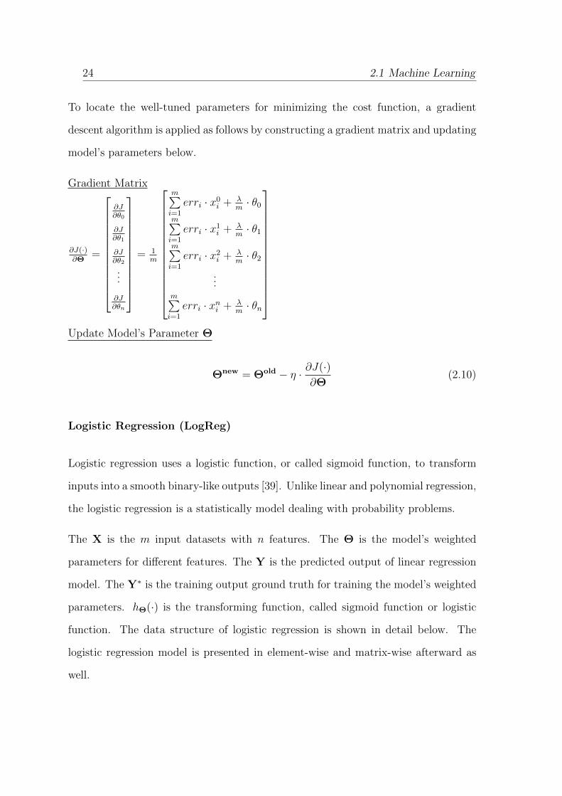
To locate the well-tuned parameters for minimizing the cost function, a gradient

22 2.1 Machine Learning
descent algorithm is applied as follows by constructing a gradient matrix and updating
model’s parameters below.
Gradient Matrix
∂J(·)∂Θ
=
∂J∂θ0
∂J∂θ1
∂J∂θ2
...
∂J∂θn
= 1
m
m∑i=1
erri · xi,0 + λm· θ0
m∑i=1
erri · xi,1 + λm· θ1
m∑i=1
erri · xi,2 + λm· θ2
...m∑i=1
erri · xi,n + λm· θn
Update Model’s Parameter Θ
Θnew = Θold − η · ∂J(·)∂Θ
(2.5)
Polynomial Regression (PolyReg)
Similar to linear regression, the polynomial regression also focus on studying the rela-
tionships between input feature and another output target. However, many problems
are not linear, but curvature in nature [62]. Therefore, there is a function needed
to fit non-linear relationship accurately. Thus the main difference is that the input
feature is not linear but polynomial terms as shown in the data structure below. That
is the reason why it is called polynomial regression. The main objective of polyno-
mial regression is to model the non-linear corresponding between independent and
dependent parameters.
The data structure of polynomial regression is presented in detail below. The X is
the m input datasets with n features. The Θ is the model’s weighted parameters for
different features. The Y is the predicted output of linear regression model. The Y∗

2.1 Machine Learning 23
is the training output ground truth for training the model’s weighted parameters.
Data Structure
X =
x01 x1
1 x21 · · · xn1
x02 x1
2 x22 · · · xn2
......
.... . .
...
x0m x1
m x2m · · · xnm
,Y =
y1
y2
...
ym
,Y∗ =
y∗1
y∗2...
y∗m
,Θ =
θ0
θ1
θ2
...
θn
Model
- Element Form [62]
yi = θ0 + θ1 · xi + θ2 · x2i + · · ·+ θn · xni (i = 1, 2, 3, · · · ,m) (2.6)
- Matrix Form [62]
Y = X ·Θ (2.7)
In order to minimize the errors of models, the cost function is defined under the
considerations of mean square error and parameter regularization below.
Cost Function
- Mean Squared Error and Regularization [57]
J(Θ|X) =1
2m
m∑i=1
(yi − y∗i )2 +λ
2m
n∑j=0
θ2j (2.8)
- Error Difference
erri = yi − y∗i (2.9)
24 2.1 Machine Learning
To locate the well-tuned parameters for minimizing the cost function, a gradient
descent algorithm is applied as follows by constructing a gradient matrix and updating
model’s parameters below.
Gradient Matrix
∂J(·)∂Θ
=
∂J∂θ0
∂J∂θ1
∂J∂θ2
...
∂J∂θn
= 1
m
m∑i=1
erri · x0i + λ
m· θ0
m∑i=1
erri · x1i + λ
m· θ1
m∑i=1
erri · x2i + λ
m· θ2
...m∑i=1
erri · xni + λm· θn
Update Model’s Parameter Θ
Θnew = Θold − η · ∂J(·)∂Θ
(2.10)
Logistic Regression (LogReg)
Logistic regression uses a logistic function, or called sigmoid function, to transform
inputs into a smooth binary-like outputs [39]. Unlike linear and polynomial regression,
the logistic regression is a statistically model dealing with probability problems.
The X is the m input datasets with n features. The Θ is the model’s weighted
parameters for different features. The Y is the predicted output of linear regression
model. The Y∗ is the training output ground truth for training the model’s weighted
parameters. hΘ(·) is the transforming function, called sigmoid function or logistic
function. The data structure of logistic regression is shown in detail below. The
logistic regression model is presented in element-wise and matrix-wise afterward as
well.

2.1 Machine Learning 25
Data Structure
X =
x1,0 x1,1 x1,2 · · · x1,n
x2,0 x2,1 x2,2 · · · x2,n
......
.... . .
...
xm,0 xm,1 xm,2 · · · xm,n
,Y =
y1
y2
...
ym
,Y∗ =
y∗1
y∗2...
y∗m
,Θ =
θ0
θ1
θ2
...
θn
Model
- Element Form
yi =1
1 + e−(θ0·xi,0+θ1·xi,1+···+θn·xi,n)(2.11)
- Matrix Form
Y = hΘ(x) =1
1 + e−X·Θ (2.12)
Since the logistic function consists of highly non-linear exponential term, the cost
function is different from those of linear and polynomial regressions with some math-
ematical manipulations illustrated below [57].
Cost Function
- Log Error and Regularization [57]
J(Θ|X) =1
m
m∑i=1
[C(hΘ(xi), y∗i )] +
λ
2m
n∑j=0
θ2j (2.13)
where
C(hΘ(xi), y∗i ) =
− ln(hΘ(xi)), if y∗i = 1
− ln(1− hΘ(xi)), if y∗i = 0
(2.14)

26 2.1 Machine Learning
Thus, Eq. 2.13 can be formulated as follows:
J(Θ|X) =−1
m
m∑i=1
[y∗i · ln(hΘ(xi)) + (1− y∗i ) · ln(1− hΘ(xi))] +λ
2m
n∑j=0
θ2j (2.15)
Gradient Matrix
∂J(·)∂Θ
=
∂J∂θ0
∂J∂θ1
∂J∂θ2
...
∂J∂θn
= −1
m
m∑i=1
[y∗i · (1− hΘ(xi))− (1− y∗i ) · hΘ(xi)] · xi,0 + λm· θ0
m∑i=1
[y∗i · (1− hΘ(xi))− (1− y∗i ) · hΘ(xi)] · xi,1 + λm· θ1
m∑i=1
[y∗i · (1− hΘ(xi))− (1− y∗i ) · hΘ(xi)] · xi,2 + λm· θ2
...m∑i=1
[y∗i · (1− hΘ(xi))− (1− y∗i ) · hΘ(xi)] · xi,n + λm· θn
Since hΘ(xi) is corresponding to yi, we have:
∂J(·)∂Θ
=
∂J∂θ0
∂J∂θ1
∂J∂θ2
...
∂J∂θn
= −1
m
m∑i=1
[y∗i · (1− yi)− (1− y∗i ) · yi] · xi,0 + λm· θ0
m∑i=1
[y∗i · (1− yi)− (1− y∗i ) · yi] · xi,1 + λm· θ1
m∑i=1
[y∗i · (1− yi)− (1− y∗i ) · yi] · xi,2 + λm· θ2
...m∑i=1
[y∗i · (1− yi)− (1− y∗i ) · yi] · xi,n + λm· θn
Update Model’s Parameter Θ
Θnew = Θold − η · ∂J(·)∂Θ
(2.16)
K Nearest Neighbors (KNN)
The K Nearest Neighbors (KNN) algorithm is a non-parametric method of super-
vised learning [9]. The KNN approach can be used for resolving both regression and

2.1 Machine Learning 27
classification problems with prior knowledge of data that is unknown or difficult to
acquire. Mostly, the KNN is a choice of classification for labeled training data [34].
Generally, the parameter “K” would be selected as an odd number, so that it can
avoid the cases of tie classification from happening.
The training data X consists of m training data sets, and each training data set has
n features with labeling Y as illustrated below. The training data outputs follow
yi ∈ C1, C2, · · · , Cs, where i ∈ [1,m] under s− class labeled.
Data Structure
X =
x1,1 x1,2 · · · x1,n
x2,1 x2,2 · · · x2,n
......
. . ....
xm,1 xm,2 · · · xm,n
,Y =
y1
y2
...
ym
Algorithm 1 K Nearest Neighbors (KNN)
1: Input: X,Y, xt2: Output: yt3: for (u = 1;u ≤ m;u+ +)
4: d(xu, xt) =
√n∑k=1
(xu,k − xt,k)2
5: endfor6: Sort d(X, xt) in ascending order up to K nearest neighbors.7: Find the highest voted classification (C∗) in K nearest neighbors(
where C∗ ∈ C1, C2, · · · , Cs)
.
8: yt ← C∗
9: Stop.
The Euclidean distance of testing data is calculated for its K nearest neighbors to
determine the final class of this particular testing data. For instance, a testing data
is xu = [xu,1, xu,2, · · · , xu,n], and its neighboring data is xv = [xv,1, xv,2, · · · , xv,n]. The

28 2.1 Machine Learning
Euclidean distance between xu and xv is therefore given as follows:
d(xu, xv) =√
(xu,1 − xv,1)2 + (xu,2 − xv,2)2 + · · ·+ (xu,n − xv,n)2 (2.17)
Based on Eq. 2.17, the confusion matrix of testing data can be calculated against all
training data. The class of testing data will be assigned as the most frequent class pre-
sented in the K nearest neighbor training data. The pseudo-code is presented in Algo-
rithm 1. (xt, yt) are input and output data for testing, where xt = [xt,1, xt,2, · · · , xt,n]
and yt ∈ C1, C2, · · · , Cs.
Neural Networks (NN)
Essentially, the learning principle is rooted in neural networks and they are widely
adopted for solving regression and classification problems [38]. Therefore, the choice
of neural networks modeling is selected and evaluated throughout the whole study.
Neural networks modeling is originated from Feed-Forward Back-Propagation net-
works. The “Feed-Forward” means that the output is the result of inputs fed with
weight coefficients forwardly. The “Back-Propagation” means that the weight coef-
ficients are trained according to the errors of outputs with respect to the associated
neurons backwardly layer by layer. There are three important stages for training
models generally. The first is to normalize the training data. The second is to for-
mulate objective function (sometimes also called cost/loss function) that is to be
minimized. The third is to derive the 1st-order differentiate equations of objective
function with respect to associated neurons [9]. Then, the neural networks models can
be trained according to the derived 1st-order differential equations and optimization
algorithms can be applied to locate the weight coefficients that result in approaching

2.1 Machine Learning 29
the minimum of the objective function. Generally, the optimal weight coefficients
are located through gradient descent methods that utilize the 1st-order differential
equations discussed previously [10].
Algorithm 2 Back Propagation (BP)
1: Input: X,Y∗,Θ(1),Θ(2), η2: Output: Θ(1),Θ(2)
3: while(stopping criteria not satisfied)4: Evaluate model output: Y5: Evaluate cost function:
6: J(Θ(2),Θ(1)|X) = 1m
m∑i=1
p∑j=1
(yi,j−y∗i,j)2+ λm
(n∑u=0
ka∑v=1
(θ(1)u,v)2+
ka∑u=0
p∑v=1
(θ(2)u,v)2
).
7: Evaluate gradient matrix:8:
∂J(·)∂Θ(2) and ∂J(·)
∂Θ(1) .
9: Update Θ(2) and Θ(1):10: Θ(2) = Θ(2) − η · ∂J(·)
∂Θ(2) , Θ(1) = Θ(1) − η · ∂J(·)∂Θ(1) .
11: endwhile12: Stop.
Σ A.F.
𝜽 𝟏
𝜽 𝟐
Σ
A.F. Σ
A.F.
Σ A.F.
Σ
+1 +1
𝑦1 𝑥1
𝑥2
𝑥𝑛
Σ 𝑦2
Σ 𝑦𝑝
𝑎1
𝑎2
𝑎3
𝑎𝑘𝑎
𝑥0 𝑎0
Input (n-feature)
Output (p-output) (𝑘𝑎-Hidden Neurons)
Figure 2.1: Topology of Neural Networks (1-Hidden Layer)-Regression
The topology of the regression neural networks as shown in Figure 2.1 above and
neural networks (1-Hidden Layer)-Regression are mathematically formulated, and

30 2.1 Machine Learning
the pseudo-code of back-propagation (BP) is provided in Algorithm 2 above. The
data structures of the regression neural networks are illustrated below. The X is
the m inputs with n features. The Y and Y∗ are the predicted outputs from the
neural networks and ground truth datasets respectively. The A(0), A(1) and A(2)
are intermediate matrices. The Θ(1) and Θ(2) are the weight parameters of neural
networks.
Data Structure
X =
x1,0 x1,1 x1,2 · · · x1,n
x2,0 x2,1 x2,2 · · · x2,n
......
.... . .
...
xm,0 xm,1 xm,2 · · · xm,n
,Y =
y1,1 y1,2 y1,3 · · · y1,p
y2,1 y2,2 y2,3 · · · y2,p
......
.... . .
...
ym,1 ym,2 ym,3 · · · ym,p
Y∗ =
y∗1,1 y∗1,2 y∗1,3 · · · y∗1,p
y∗2,1 y∗2,2 y∗2,3 · · · y∗2,p...
......
. . ....
y∗m,1 y∗m,2 y∗m,3 · · · y∗m,p
,A(0) =
a1,0
a2,0
...
am,0
,A(1) =
a1,1 a1,2 · · · a1,ka
a2,1 a2,2 · · · a2,ka
......
. . ....
am,1 am,2 · · · am,ka
A(2) =
[A(0) A(1)
], where ai,0 = 1 for ∀ i ∈ [1,m] and i ∈ Z+
Θ(1) =
θ(1)0,1 θ
(1)0,2 θ
(1)0,3 · · · θ
(1)0,ka
θ(1)1,1 θ
(1)1,2 θ
(1)1,3 · · · θ
(1)1,ka
......
.... . .
...
θ(1)n,1 θ
(1)n,2 θ
(1)n,3 · · · θ
(1)n,ka
,Θ(2) =
θ(2)0,1 θ
(2)0,2 θ
(2)0,3 · · · θ
(2)0,p
θ(2)1,1 θ
(2)1,2 θ
(2)1,3 · · · θ
(2)1,p
......
.... . .
...
θ(2)ka,1 θ
(2)ka,2 θ
(2)ka,3 · · · θ
(2)ka,p
Activation Function (Sigmoid Function)
h(x) =1
1 + e(−x)(2.18)

2.1 Machine Learning 31
Model
- Element Form
ai,k =1
1 + e−(xi,0·θ(1)0,k+xi,1·θ
(1)1,k+···+xi,n·θ
(1)n,k)
(2.19)
where i = 1, 2, 3, · · · ,m and k = 1, 2, 3, · · · , ka.
yi,j = ai,0 · θ(2)0,j + ai,1 · θ(2)
1,j + · · ·+ ai,ka · θ(2)ka,j (2.20)
where i = 1, 2, 3, · · · ,m and j = 1, 2, 3, · · · , p.
- Matrix Form
A(1) = h
(X ·Θ(1)
)(2.21)
Y = A(2) ·Θ(2) (2.22)
Cost Function
J(Θ(2),Θ(1)|X) =1
m
m∑i=1
p∑j=1
(yi,j−y∗i,j)2+λ
m
( n∑u=0
ka∑v=1
(θ(1)u,v)
2+ka∑u=0
p∑v=1
(θ(2)u,v)
2
)(2.23)
erri,j = yi,j − y∗i,j (2.24)
Gradient Matrix

32 2.1 Machine Learning
∂J(·)∂Θ(2) =
∂J
∂θ(2)0,1
∂J
∂θ(2)0,2
∂J
∂θ(2)0,3
· · · ∂J
∂θ(2)0,p
∂J
∂θ(2)1,1
∂J
∂θ(2)1,2
∂J
∂θ(2)1,3
· · · ∂J
∂θ(2)1,p
......
.... . .
...
∂J
∂θ(2)ka,1
∂J
∂θ(2)ka,2
∂J
∂θ(2)ka,3
· · · ∂J
∂θ(2)ka,p
, ∂J(·)∂Θ(1) =
∂J
∂θ(1)0,1
∂J
∂θ(1)0,2
∂J
∂θ(1)0,3
· · · ∂J
∂θ(1)0,ka
∂J
∂θ(1)1,1
∂J
∂θ(1)1,2
∂J
∂θ(1)1,3
· · · ∂J
∂θ(1)1,ka
......
.... . .
...
∂J
∂θ(1)n,1
∂J
∂θ(1)n,2
∂J
∂θ(1)n,3
· · · ∂J
∂θ(1)n,ka
where
∂J
∂θ(2)0,1
= 2m
m∑i=1
erri,1 · ai,0 + 2λm· θ(2)
0,1
· · ·∂J
∂θ(2)0,p
= 2m
m∑i=1
erri,p · ai,0 + 2λm· θ(2)
0,p
· · ·∂J
∂θ(2)ka,1
= 2m
m∑i=1
erri,1 · ai,ka + 2λm· θ(2)
ka,1
· · ·∂J
∂θ(2)ka,p
= 2m
m∑i=1
erri,p · ai,ka + 2λm· θ(2)
ka,p
and
∂J
∂θ(1)0,1
= 2m
m∑i=1
p∑j=1
erri,j · θ(2)1,j · ai,1 · (1− ai,1) · xi,0 + 2λ
m· θ(1)
0,1
· · ·∂J
∂θ(1)0,ka
= 2m
m∑i=1
p∑j=1
erri,j · θ(2)ka,j · ai,ka · (1− ai,ka) · xi,0 + 2λ
m· θ(1)
0,ka
· · ·∂J
∂θ(1)n,1
= 2m
m∑i=1
p∑j=1
erri,j · θ(2)1,j · ai,1 · (1− ai,1) · xi,n + 2λ
m· θ(1)
n,1
· · ·∂J
∂θ(1)n,ka
= 2m
m∑i=1
p∑j=1
erri,j · θ(2)ka,j · ai,ka · (1− ai,ka) · xi,n + 2λ
m· θ(1)
n,ka
The topology of the classification neural networks as shown in Figure 2.2 with neural
networks (1-Hidden Layer)-Classification are mathematically formulated. The data

2.1 Machine Learning 33
structures of classification neural networks are illustrated below. The X is the m
inputs with n features. The Y and Y∗ are the predicted outputs from the neu-
ral networks and ground truth datasets respectively. The A(0), A(1) and A(2) are
intermediate matrices. The Θ(1) and Θ(2) are the weight parameters shown below.
Σ A.F.
𝜽 𝟏
𝜽 𝟐
Σ
A.F. Σ
A.F.
Σ A.F.
Σ
+1 +1
𝑦1 𝑥1
𝑥2
𝑥𝑛
Σ 𝑦2
Σ 𝑦𝑝
𝑎1
𝑎2
𝑎3
𝑎𝑘𝑎
𝑥0 𝑎0
Input (n-feature)
Output (p-output) (𝑘𝑎-Hidden Neurons)
A.F.
A.F.
A.F.
Figure 2.2: Topology of Neural Networks (1-Hidden Layer)-Classification
Data Structure
X =
x1,0 x1,1 x1,2 · · · x1,n
x2,0 x2,1 x2,2 · · · x2,n
......
.... . .
...
xm,0 xm,1 xm,2 · · · xm,n
,Y =
y1,1 y1,2 y1,3 · · · y1,p
y2,1 y2,2 y2,3 · · · y2,p
......
.... . .
...
ym,1 ym,2 ym,3 · · · ym,p
Y∗ =
y∗1,1 y∗1,2 y∗1,3 · · · y∗1,p
y∗2,1 y∗2,2 y∗2,3 · · · y∗2,p...
......
. . ....
y∗m,1 y∗m,2 y∗m,3 · · · y∗m,p
,A(0) =
a1,0
a2,0
...
am,0
,A(1) =
a1,1 a1,2 · · · a1,ka
a2,1 a2,2 · · · a2,ka
......
. . ....
am,1 am,2 · · · am,ka

34 2.1 Machine Learning
A(2) =
[A(0) A(1)
], where ai,0 = 1 for ∀ i ∈ [1,m] and i ∈ Z+
Θ(1) =
θ(1)0,1 θ
(1)0,2 θ
(1)0,3 · · · θ
(1)0,ka
θ(1)1,1 θ
(1)1,2 θ
(1)1,3 · · · θ
(1)1,ka
......
.... . .
...
θ(1)n,1 θ
(1)n,2 θ
(1)n,3 · · · θ
(1)n,ka
,Θ(2) =
θ(2)0,1 θ
(2)0,2 θ
(2)0,3 · · · θ
(2)0,p
θ(2)1,1 θ
(2)1,2 θ
(2)1,3 · · · θ
(2)1,p
......
.... . .
...
θ(2)ka,1 θ
(2)ka,2 θ
(2)ka,3 · · · θ
(2)ka,p
Activation Function (Sigmoid Function)
h(x) =1
1 + e(−x)(2.25)
Model
- Element Form
ai,k =1
1 + e−(xi,0·θ(1)0,k+xi,1·θ
(1)1,k+···+xi,n·θ
(1)n,k)
(2.26)
where i = 1, 2, 3, · · · ,m and k = 1, 2, 3, · · · , ka.
yi,j =1
1 + e(ai,0·θ(2)0,j+ai,1·θ
(2)1,j+···+ai,ka·θ
(2)ka,j)
(2.27)
where i = 1, 2, 3, · · · ,m and j = 1, 2, 3, · · · , p.
- Matrix Form
A(1) = h
(X ·Θ(1)
)(2.28)
Y = h
(A(2) ·Θ(2)
)(2.29)

2.1 Machine Learning 35
Cost Function
J(Θ(2),Θ(1)|X) =1
m
m∑i=1
p∑j=1
(yi,j−y∗i,j)2+λ
m
( n∑u=0
ka∑v=1
(θ(1)u,v)
2+ka∑u=0
p∑v=1
(θ(2)u,v)
2
)(2.30)
erri,j = yi,j − y∗i,j (2.31)
Gradient Matrix
∂J(·)∂Θ(2) =
∂J
∂θ(2)0,1
∂J
∂θ(2)0,2
∂J
∂θ(2)0,3
· · · ∂J
∂θ(2)0,p
∂J
∂θ(2)1,1
∂J
∂θ(2)1,2
∂J
∂θ(2)1,3
· · · ∂J
∂θ(2)1,p
......
.... . .
...
∂J
∂θ(2)ka,1
∂J
∂θ(2)ka,2
∂J
∂θ(2)ka,3
· · · ∂J
∂θ(2)ka,p
, ∂J(·)∂Θ(1) =
∂J
∂θ(1)0,1
∂J
∂θ(1)0,2
∂J
∂θ(1)0,3
· · · ∂J
∂θ(1)0,ka
∂J
∂θ(1)1,1
∂J
∂θ(1)1,2
∂J
∂θ(1)1,3
· · · ∂J
∂θ(1)1,ka
......
.... . .
...
∂J
∂θ(1)n,1
∂J
∂θ(1)n,2
∂J
∂θ(1)n,3
· · · ∂J
∂θ(1)n,ka
where
∂J
∂θ(2)0,1
= 2m
m∑i=1
erri,1 · yi,1 · (1− yi,1) · ai,0 + 2λm· θ(2)
0,1
· · ·∂J
∂θ(2)0,p
= 2m
m∑i=1
erri,p · yi,p · (1− yi,p) · ai,0 + 2λm· θ(2)
0,p
· · ·∂J
∂θ(2)ka,1
= 2m
m∑i=1
erri,1 · yi,1 · (1− yi,1) · ai,ka + 2λm· θ(2)
ka,1
· · ·∂J
∂θ(2)ka,p
= 2m
m∑i=1
erri,p · yi,p · (1− yi,p) · ai,ka + 2λm· θ(2)
ka,p
and
∂J
∂θ(1)0,1
= 2m
m∑i=1
p∑j=1
erri,j · yi,j · (1− yi,j) · θ(2)1,j · ai,1 · (1− ai,1) · xi,0 + 2λ
m· θ(1)
0,1
· · ·∂J
∂θ(1)0,ka
= 2m
m∑i=1
p∑j=1
erri,j · yi,j · (1− yi,j) · θ(2)ka,j · ai,ka · (1− ai,ka) · xi,0 + 2λ
m· θ(1)
0,ka

36 2.1 Machine Learning
· · ·∂J
∂θ(1)n,1
= 2m
m∑i=1
p∑j=1
erri,j · yi,j · (1− yi,j) · θ(2)1,j · ai,1 · (1− ai,1) · xi,n + 2λ
m· θ(1)
n,1
· · ·∂J
∂θ(1)n,ka
= 2m
m∑i=1
p∑j=1
erri,j · yi,j · (1− yi,j) · θ(2)ka,j · ai,ka · (1− ai,ka) · xi,n + 2λ
m· θ(1)
n,ka
Deep Learning (DL)
Aforementioned Neural Networks (NN) is a part of essential architectures for Deep
Learning (DL) [33]. As its name implies, a deep learning architecture consists of deep
hidden layers between inputs and outputs, which basically are deep neural networks.
Among each layer, there are different types of topologies, such as partially or fully
connected. Similarly, all data for training is labeled (i.e. a supervised learning with a
large number of neurons and parameters to be tuned). Due to its complex layer archi-
tectures, each layer could learn some new abstract features from its inputs layer, and
thus could generate more meaningful outputs for the next layer to process. Generally,
deep learning has excellent performance in solving pattern recognition, classification,
image processing and computer vision problems [33]. It can even be combined with
reinforcement learning for competing chess games and artificial intelligence gaming
strategy.
Moreover, traditional feature extractions of neural networks are on the basis of man-
ual differentiations. After the features are extracted, the parameters of weights are
trained so as to minimize the cost function. However, deep learning completes feature
extraction within its deep hidden layers of neural networks without the prior knowl-
edge of the facing problems. Many abstract features extracted are not identified by
human beings after a series of complex computations and transformations. One of

2.1 Machine Learning 37
the most commonly used networks in deep learning is Convolutional Neural Networks
(CNN). Normally, a 2D filter is selected for the convolution computations, and the
best application is for 2D data sets, such as image. For example, there is a picture
of circle. The first layer could detect edges features, and deeper hidden layers could
detect some more feature like eccentricity. Then the final layer could tell whether it
is a square, rectangle, triangle or circle. Another example is shown in Figure 2.3 to
illustrate the identification of a bird in an image. This model is fed and trained with
many other labeled data sets, such as images of cats, dogs, etc [59, 97].
Figure 2.3: Convolutional Neural Networks (CNN) on Bird Classification
Besides the aforementioned applications, deep learning also performs excellently in
many other fields, such as Natural Language Process (NLP), robotics, Computer
Visions (CV), search engine, advertisement pop-up, medical diagnosis, financial pre-
diction, etc.
2.1.3 Unsupervised Learning
Compared to supervised learning, unsupervised learning extracts information from
unlabeled training data sets. Therefore, the unsupervised learning is mainly for clus-
tering problem, while not for regression and classification problems like supervised

38 2.1 Machine Learning
learning [13]. Unsupervised learning essentially analyzes the feature extractions and
selections of unlabeled training data sets. There are many state-of-the-art unsu-
pervised learning algorithms, such as K-Means, Hierarchical Clustering, Principal
Component Analysis (PCA), Self Organization Maps (SOM), etc [10].
Hierarchical Clustering
There are three categories of clustering techniques, and they are hierarchical-based,
partitional-based and Bayesian-based. In hierarchical clustering technique, successive
clusters are determined by its previously established clusters. There are two kinds of
sub-groups in hierarchical clustering based on propagation directions. One is called
“Top-Bottom” architecture that means smaller successive clusters are further divided
from larger previous clusters. Another architecture is followed as “Bottom-Top” that
means larger successive clusters are aggregated from smaller previous clusters.
1. Top-Bottom:
Start with all data in one cluster, the root.
Split the root into several children clusters, and each child is further recursively
divided.
Stop when each cluster contains single data.
2. Bottom-Top:
Start with bottom single data.
Merge the most similar data into one cluster, and most similar clusters into a
new cluster.
Stop when all the data are merged into one single cluster.

2.1 Machine Learning 39
The similarity of two adjacent data or clusters can be monitored by Euclidean dis-
tance, Manhattan distance or Minkowski distance. A larger distance means that the
similarity is less between each other.
The Euclidean distance is defined as follows:
dist(xi, xj) =
√√√√ n∑k=1
(x(k)i − x
(k)j )2 (2.32)
The Manhattan distance is defined as follows:
dist(xi, xj) =n∑k=1
|x(k)i − x
(k)j | (2.33)
The Minkowski distance is defined as follows:
distp(xi, xj) =
( n∑k=1
|x(k)i − x
(k)j |p
) 1p
(2.34)
where p is a positive integer.
K-Means
K-Means algorithm of clustering was first proposed by MacQueen in 1967, and it is
a type of partitional clustering technique using the centroid approach. There are K
centroids (i.e. K clustering) spread out in the data space, and each centre of one
cluster is called a centroid, and it is calculated by the mean of this particular cluster
of data among the data space [40], The pseudo-code is illustrated in Algorithm 3.
There are some stopping criteria to be noted as well in the pseudo-code. In order to
differentiate whether the iterations have converged, one uses the positions of centroids

40 2.1 Machine Learning
to indicate. If the positions of centroids are not changing or changing at a very
minimal level, then the iterations can be stopped and the clusters are indicated as
having converged.
Similar to neural networks, the input training datasets X are following the data
structure as below. There are m different datasets and each dataset consists of n
features.
Data Structure
X =
x1,1 x1,2 · · · x1,n
x2,1 x2,2 · · · x2,n
......
. . ....
xm,1 xm,2 · · · xm,n
Algorithm 3 K-Means1: Input: X2: Choose K random data from X as initial centroids.3: while(stopping criteria not satisfied)4: Assign data into their nearest centroid clusters.5: Euclidean distance can be calculated as follows:
6: dist(xi, xj) =
√n∑k=1
(xi,k − xj,k)2
7: Re-calculate centroids with current data clusters.8: endwhile9: Stop.
There are many advantages in K-Means algorithm. First, it is a linear algorithm
under O(tkm), where t is the number of iterations, k is the number of clusters and m
is the number of data points. Second, it is easy to implement due to its simplicity and
efficiency. However, there are some limitations as well. For instance, the clustering
results will be heavily impacted by outliers or mis-leading data, since the algorithm
considers every single data for clustering. Moreover, the initial randomly selected
centroids will be leading to significantly divergent clustering results. Even though

2.1 Machine Learning 41
there are drawbacks in the K-Means algorithm, it is still the most popular clustering
algorithm and there is no clear evidence showing that any other clustering algorithm
performs better in general.
Principal Component Analysis (PCA)
Principal Component Analysis (PCA) is a statistical procedure that uses an orthog-
onal transformation to convert a set of observations of possibly correlated variables
into a set of values of linearly uncorrelated variables [69], and the linearly uncor-
related variables are called principal components. The pseudo-code is presented in
Algorithm 4.
Algorithm 4 Principal Component Analysis (PCA)
1: Input: X2: Output: X
′
3: Standardize X into X0 by means centering.4: Compute covariance matrix (C) of the standardized data X0.5: Compute eigenvalues (D) and eigenvectors (V) of the covariance matrix.6: Rank D and V in descending order of eigenvalues into D∗ and V∗.7: Transpose V∗ and reduce k rows from bottom into VPCA.
8: Calculate decomposed data: X′=
(VPCA ·XT
)T9: Stop.
The m datasets with n features are formulated as matrix X below. The mean values of
different features are calculated and presented in matrix µ, and the basic formulation
is illustrated as follows [2].
Data Structure

42 2.1 Machine Learning
X =
x1,1 x1,2 · · · x1,n
x2,1 x2,2 · · · x2,n
......
. . ....
xm,1 xm,2 · · · xm,n
,µ =
[µ1 µ2 · · · µn
], where µk = 1
m
m∑i=1
xi,k
X0 =
(x1,1 − µ1) (x1,2 − µ2) · · · (x1,n − µn)
(x2,1 − µ1) (x2,2 − µ2) · · · (x2,n − µn)
......
. . ....
(xm,1 − µ1) (xm,2 − µ2) · · · (xm,n − µn)
Covariance matrix of the standardized data X0:
C =1
m·X0
T ·X0 (2.35)
Eigenvalues and eigenvectors of covariance matrix C:
D =
λ1 0 · · · 0
0 λ2 · · · 0
......
. . ....
0 0 · · · λn
,V =
V(1)
1 V(2)
1 · · · V(n)
1
V(1)
2 V(2)
2 · · · V(n)
2
......
. . ....
V(1)n V
(2)n · · · V
(n)n
Rank D and V in descending order of eigenvalues, we get D→ D∗, V→ V∗.
Transpose the ranked eigenvectors V∗ and reduce k rows of vectors from bottom:
V∗T =
V(1)
1 V(1)
2 · · · V(1)n
V(2)
1 V(2)
2 · · · V(2)n
......
. . ....
V(n)
1 V(n)
2 · · · V(n)n
⇒ VPCA =
V(1)
1 V(1)
2 · · · V(1)n
V(2)
1 V(2)
2 · · · V(2)n
......
. . ....
V(n−k)
1 V(n−k)
2 · · · V(n−k)n

2.1 Machine Learning 43
Reduce k features (dimensions) from n features (X→ X′):
X′=
(VPCA ·XT
)T(2.36)
The data obtained in X′
is the standardized and linearly uncorrelated data with k
feature reduced. The data X′
is orthogonally decomposed and transformed into a
lower dimension space. Thus the PCA algorithm essentially achieves the purpose of
features’ dimension reduction.
2.1.4 Reinforcement Learning
Besides supervised and unsupervised learning techniques, another main branch of
learning techniques is reinforcement learning (RL). The reinforcement learning is
most similar to our natural processes of learning. There are agent and environment
that will interact with each other [73]. The agent is like a human being, who is
responsible to take actions towards the environment. The environment receives the
corresponding actions and generates reward or penalty back to the agent, while it also
changes its current state accordingly. It is like teaching a baby to perform correct
doings by providing some candy or fruit as a reward, and punishing the baby by
taking aways some candy or fruit as a penalty if some wrong deeds are conducted.
In the domain of reinforcement learning, returns are the summation of rewards. The
agent will adjust its strategy accordingly to achieve maximum returns in the long-term
[73]. The returns (Rt) at time t are defined as follows:
Rt = rt+1 + γ · rt+2 + γ2 · rt+3 + · · · =inf∑k=0
γk · rt+k+1 (2.37)

44 2.1 Machine Learning
where γ is the discount rate in the range of [0, 1].
There are three classifications regarding on different ranges of γ. For γ = 0, the agent
is called “myopic agent” that only maximizes immediate rewards. For 0 < γ < 1,
Rt is a finite sum as long as the series rk is bounded. For γ → 1, the agent is a
farsighted agent that takes future long-term rewards more strongly into account.
According to the theory of reinforcement learning rooted in Markov Decision Process
(MDP), a policy (π(s, a)) is a probability distribution with respect to action (a) under
state (s). The State-Value function under policy π is shown as follows:
V π(s) = Eπ
Rt|st = s
= Eπ
inf∑k=0
γk · rt+k+1|st = s
=∑a
π(s, a)∑s′
P ass′
(Rass′ + γ · V π(s′)
) (2.38)
The Action-Value function under policy π is presented as follows:
Qπ(s, a) = Eπ
Rt|st = s, at = a
= Eπ
inf∑k=0
γk · rt+k+1|st = s, at = a
=∑s′
P ass′
(Rass′ + γ · V π(s′)
) (2.39)
In reinforcement learning, an optimal solution is obtained if there is a policy (π)
found that it can achieve the maximum level of rewards over a long-term running.
Therefore, the optimal State-value is V ∗(s) = maxπ
V π(s) for ∀s ∈ S, and the optimal
Action-value is Q∗(s, a) = maxπ
Qπ(s, a) for ∀s ∈ S,∀a ∈ A(s) [73].

2.1 Machine Learning 45
In order to locate an optimal policy solution, there are a series of policy iterations to
be conducted. It consist of policy evaluation and policy improvement in each time of
iteration. The pseudo-code [73] of policy iteration is illustrated in Algorithm 5.
Algorithm 5 Policy Iteration
1: 1. Initialization:2: V (s) ∈ R, π(s) ∈ A(s) arbitrarily ∀s ∈ S.3: 2. Policy Evaluation:4: Repeat5: ∆← 06: for each s ∈ S:7: v ← V (s)
8: V (s)←∑s′Pπ(s)ss′
(Rπ(s)ss′ + γ · V (s′)
)9: ∆← max(∆, |v − V (s)|)10: Until ∆ < θ, where θ is a small positive number11: 3. Policy Improvement:12: policy stable ← true13: for each s ∈ S:14: b← π(s)
15: π(s)← arg maxa
∑s′P ass′
(Rass′ + γ · V (s′)
)16: If b 6= π(s), then policy stable ← false.17: If policy stable is true, then stop;18: Else go to section 2.19: Stop.
2.1.5 Summary
In this section, we have examined different and widely applied machine learning tech-
niques, such as supervised learning, unsupervised learning and reinforcement learning.
The supervised learning mainly covers linear regression, polynomial regression, logis-
tic regression, k nearest neighbors, neural networks, etc. The supervised learning can
provide a higher accuracy in labeled data sets for training, compared to unsupervised
learning in classification or clustering problems. It is mainly discussed over hierarchi-

46 2.1 Machine Learning
cal clustering, k means, principal component analysis, etc in unsupervised learning.
As for the reinforcement learning, the basic principles of policy evaluation, policy im-
provement and policy determination are illustrated, and agent-environment loops of
action-reward are discussed. The theory and application methods of different machine
learning techniques are elaborated with respect to different types of problems.

2.2 Thermal Comfort 47
2.2 Thermal Comfort
In this section, different approaches of evaluating indoor thermal comfort sensations
are examined. The approaches examined are based on environmental and physiologi-
cal occupant models, and also data-driven machine learning models. The data-driven
models can be further divided into three groups. The first group uses only the envi-
ronmental parameters to train thermal comfort models [26]. The second group uses
only occupant parameters to train thermal comfort models [21]. The last group is a
hybrid model that can be trained by environmental and occupant parameters [95].
The environmental parameters in the hybrid models are to be used as a tuning factor
to adjust thermal comfort model more accurately. In this study, only the first and
second groups are elaborated and discussed in details.
2.2.1 Introduction
Generally, people spend about 90% of their time staying in indoor environment [56].
A thermally comfortable environment would make occupants more productive and
healthier for both workplace and home. According to the ISO 7730 standard, the
definition of “thermal comfort” is that of “the condition of mind which expresses
satisfaction with the thermal environment” [6]. However, the evaluations of thermal
comfort are far more complex than this simple definition.
There are many parameters to be considered environmentally and physiologically in
order to thoroughly describe the conditions of thermal comfort in an environment [6].
Environmentally, there are parameters such as air flow rate, temperature, humidity,
pressure, velocity, solar radiation, light, air quality, noise, etc. Physiologically, the
condition of occupants matters and it can impact their thermal comfort satisfactions.

48 2.2 Thermal Comfort
These include the activity levels of occupants, clothing status, genders, etc [74].
2.2.2 Passive Approach
The passive approach to explore thermal comfort sensations is by using objective
environmental conditions. The environmental conditions generally consist of air field
conditions, radiation conditions and occupant objective conditions. As for air field
conditions, there are many parameters to be considered, such as air flow rate, air
temperature, air relative humidity, air quality, air pressure, air velocity, etc [6]. The
radiation conditions are basically the result of solar radiation of the day. Thus, there
is a need to also include the occupant objective parameters, such as clothing factor,
metabolic rate, activity level, etc [6].
The most famous and well adopted approach was originated from P. O. Fanger in
1970s [26, 42, 72]. He proposed innovative Predicted Mean Vote (PMV) model and
Predicted Percentage of Dissatisfied (PPD) model to predict thermal comfort sensa-
tions of occupants from a series of physical laws and large amount of occupant surveys
[26]. Based on the study, there are two conditions to be satisfied so as to be thermally
comfortable for occupants. Condition 1 is a sense of thermal neutrality achieved from
skin temperature and the body’s core temperature. Condition 2 is the heat balance of
a body, which means the heat generated by metabolic processes of the body is equal
to the heat lost from the body [76].
According to ISO-7730:2005, the Fanger’s PMV model [75] is elaborated as follows:
PMV =
(0.303 · e−0.036M + 0.028
)·(M −W −Q
)(2.40)

2.2 Thermal Comfort 49
where
Q = Qdiff +Qevap +Qresp,
Qdiff = 3.05×10−3 ·[5733−6.99 · (M −W )−Pa
]− 1
Icl
[Tcl−35.7+0.028 · (M −W )
],
Qevap = 0.42 · (M −W − 58.15),
Qresp = 1.71× 10⁻⁵ ·M · (5869− Pa) + 0.0014 ·M · (34− Ta),
Tcl = 35.7− 0.028 · (M −W )− Icl
3.96× 10⁻⁸ · fcl ·[(Tcl + 273)4 − (Tmr + 273)4
]+
fcl · hc · (Tcl − Ta)
,
hc = max
2.38 · |Tcl − Ta|1/4
12.1 ·√Va
fcl =
1.00 + 1.29 · Icl, (Icl ≤ 0.078m2K/W.)
1.05 + 0.645 · Icl, (Icl > 0.078m2K/W.)
Pa = 6.11 · RH100· 10
7.5·Ta237.7+Ta .
PPD = 100− 95 · e−(0.03353·PMV 4+0.2179·PMV 2) (2.41)
In Eq. 2.40 of the PMV model, Qdiff is the heat loss by diffusion of an occupant,
and Qevap and Qresp are the heat losses by evaporation and respiration processes
respectively. The Predicted Percentage of Dissatisfied (PPD) model in Eq. 2.41 is
highly related to the PMV model. However, due to different people and environmental
conditions, the models of PMV and PPD have to be calibrated so as to achieve better
performance.

50 2.2 Thermal Comfort
2.2.3 Active Approach
The active approach to examine thermal comfort sensations is through the evaluations
of subjective occupant conditions [21, 71, 83]. The information of subjective occupant
conditions are gender, clothing, skin temperatures of different spots of the body,
blood pressure, etc. Furthermore, the gradient of such physiological parameters can
also be parts of the important information [16, 32]. After a large amount of research
[52], it has been shown that skin temperature is the most significant physiological
parameter to the thermal comfort sensations of occupants [19]. In addition, its first
order gradient is also an important input for providing the rate of change and its
changing trends.
There are many skin spots that have been evaluated for thermal comfort sensations
in the previous studies and they are as shown in Figure 2.4. According to the fig-
ure, each spot of the skin is labeled as “A: forehead, B: chest, C: upper arm, D:
back, E: abdomen, F: elbow, G: hand, H: anterior thigh, I: anterior calf, J: foot”
correspondingly.
Figure 2.4: Human Skin Spots for Thermal Comfort Sensation Evaluations [53]

2.2 Thermal Comfort 51
For the active approaches, they can be further divided into two general groups of
multiple skin-spot and single skin-spot approaches [17]. The multiple skin-spot ap-
proach basically transfers multiple skin temperature into a single weighted average of
skin temperature [89]. For example, Liu et. al. [53] had used this approach via Eq.
2.42:
Tsk = 0.06Tforehead + 0.08Tupperarm + 0.06Telbow
+ 0.05Thand + 0.12Tback + 0.12Tchest
+ 0.12Tabdomen + 0.19Tthigh + 0.13Tcalf + 0.07Tfoot
(2.42)
The single skin-spot approach is normally utilizing the skin temperatures of wrist
or the hand’s back parts and their corresponding gradients as research had shown
the significant improvements on thermal comfort sensation modelings. Besides skin
temperature, there are many other physiological parameters to be addressed, such as
hight, weight, gender, etc [74]. These parameters are used to further standardize skin
temperature and to keep the features more generally comparable.
Since some physiological parameters (i.e. height and weight) are also important to
skin temperature, a normalization factor is developed as well for better data repre-
sentations as Eq. 2.44 shows, and the normalized skin temperature is calculated as
Eq. 2.43:
Tsk = Thand
Tsk,norm =TskAnorm
(2.43)

52 2.2 Thermal Comfort
where
Anorm = (1− Icl) · Adu
Adu = Weight0.425 ×Height0.725 × 0.203
(2.44)
2.2.4 Summary
In this section, different approaches for thermal comfort evaluations are examined.
There are two approaches to evaluate thermal comfort levels, namely passive and
active approaches. The passive approaches extract the information largely from envi-
ronmental parameters, such as air temperature, air flow rate, air velocity, air relative
humidity, air pressure, etc. The active approaches predict thermal comfort sensa-
tions by measuring the physiological parameters of occupants directly. The passive
approaches are non-intrusive to occupants, however, they generally involve high cost
of sensory implementation and measurement. The active approaches are easy to im-
plement, but the personal physiological data of occupants may be at risk of exposure.
But this cannot prevent the active approaches from becoming a promising and fea-
sible technology in real applications, especially when one can proposed a simple and
easily implementable physiological measurement through secure data channels.

2.3 Optimization Algorithms 53
2.3 Optimization Algorithms
In this section, different optimization algorithms are examined and discussed. The
optimization algorithms are grouped into three categories, namely nature-inspired,
Bayesian-based and analytical algorithms. In the category of nature-inspired algo-
rithms, some famous algorithms examined are the genetic algorithm, particles swarm
optimization and augmented firefly algorithm [85]. In the category of Bayesian-based
algorithm, a special Bayesian Gaussian Process optimization are evaluated [61]. Last-
ly, the analytical method algorithms such as gradient descent methods, quadratic
optimization are examined [11].
2.3.1 Introduction
There are many optimization theory and algorithms for solving optimization prob-
lems. Most of practical problems that we face are not solvable through analytical
methods [11, 23]. Therefore, probability-based and numerical-based methods can be
used as alternative approaches for solving highly non-linear, discrete or continuous
optimization problems [81].
2.3.2 Genetic Algorithm
The genetic algorithm (GA) that was developed by John H. Holland and his col-
leagues in 1970s [38] is one of the most widely applied algorithms. The basic idea
of genetic algorithm is based on the evolutionary theory of Charles Darwin’s natural
selection. According to Darwin’s theory, the biological evolution consists of opera-
tors like crossover, mutation, recombination and selection. These operators in genetic
algorithms are essential components to mimic the natural process of biology.

54 2.3 Optimization Algorithms
According to the schemes of genetic algorithm, the procedures can be briefly illus-
trated as follows: 1) define cost function, 2) define fitness function, 3) create initial
population, 4) perform iteration or evolution to generate new population by crossover,
mutation and recombination, 5) decode the final solution based on selection criteria.
To be more specific, the pseudo-code is as presented in Algorithm 6.
Algorithm 6 Genetic Algorithm
1: Define objective function2: f(x), x = (x1, x2, · · · , xd)T3: Encode solutions into chromosomes4: Define fitness function5: F ∝ f(x) for maximization problems6: Generate initial population7: Initialize crossover(pc) and mutation(pm) probabilities8: while t ≤Max Generation:9: Generate new solutions by crossover and mutation10: Accept the new solutions if fitness values increase11: Select current best solution for the next generation (elitism)12: Update t← t+ 113: endwhile14: Visualization results15: Stop.
As mentioned previously, there are three main essential operators and they are crossover,
mutation and selection. For crossover, it operates the swapping between chromosomes
which means mixing partial solutions happen over this operation under a probability
pc. Similarly for mutation, it performs the information changes of chromosomes which
means solutions change randomly under a probability pm. This operation can avoid
being trapped into a local optimum. Moreover, the selection operator follows the
principle of Darwin’s “fittest of the survival”, and it operates as a natural selection
process over the population or solutions. The fittest solutions will be the survival into
the next generation. After a few number of generations, solutions will be converging
to the final output results.

2.3 Optimization Algorithms 55
2.3.3 Particle Swarm Optimization
Particle swarm optimization (PSO) was firstly developed from nature inspiration by
Kennedy and Eberhart in 1995 [41]. The PSO is inspired by swarm behaviors in
biological activities, such as fish and bird schooling [85]. According to many reviews,
PSO has been applied into almost every field of optimizations, and there are many
transformed and hybrid versions of PSO as well, and the pseudo-code for particle
swarm optimization is illustrated in Algorithm 7.
Algorithm 7 Particle Swarm Optimization
1: Define objective function2: f(x), x = (x1, x2, · · · , xd)T3: Initialize locations xi and velocity vi of n particles
4: Find g∗ from min
f(x1), · · · , f(xn)
(at t = 0)
5: while (criteria):6: for loop all n particles and all d dimensions:7: Generate new velocity8: vt+1
i = vti + α · ε1(g∗ − xti) + β · ε2(x∗(t)i − xti)
9: Calculate new location10: xt+1
i = xti + vt+1i
11: Evaluate new locations xt+1i by objective function
12: Find the current best for each particle x∗i13: endfor14: Find the current global best g∗
15: Update t← t+ 116: endwhile17: Visualize results x∗i and g∗
18: Stop.
The particle swarm optimization considers each particle as a solution to the particular
optimization problem. The particles (i.e. solutions) will be swarming or converging
into optima after numerous iterations. As Figure 2.5 shows, the particle i will proceed
on many possible directions. However, it may be going toward current optimum x∗i ,

56 2.3 Optimization Algorithms
but it eventually will approach g∗ (i.e. global optimum).
Figure 2.5: Particle Swarm Optimization Principle
Based on the studies of X. S. Yang [87], particle swarm optimization can perform
outstandingly over many other optimization algorithms, such as genetic algorithm
and other conventional algorithms. However, there are still drawbacks, such as pre-
mature convergence and trapped into local optima. As mentioned by X. S. Yang
[87] in the book, many other methods, namely cuckoo search method and firefly
algorithms, also outperform PSO algorithms in many applications.
2.3.4 Firefly Algorithm
The study of nature-inspired optimization algorithms has been surging over the last
10-15 years. In the meantime, firefly algorithms (FA) have emerged since 2008 [87].
Due to their properties of efficiency and fast convergence, the research under this
topic has been very popular and have drawn significant attentions.
The first firefly algorithm is described in the published papers of X. S. Yang in 2008
[85, 86]. For simplicity, some rules are to be defined as follows: 1) All fireflies are
unisex, so the attractiveness of each other is regardless of sex; 2) Attractiveness is
proportional to the brightness of firefly. The brightness is decreasing as the distance
between each other increases. If there is no brighter one, fireflies will be wandering

2.3 Optimization Algorithms 57
randomly; 3) The brightness is governed by the objective function. The pseudo-code
of firefly algorithm is presented in Algorithm 8.
Algorithm 8 Firefly Algorithm
1: Define objective function2: f(x), x = (x1, x2, · · · , xd)T3: Initialize population of n fireflies xi (i = 1, 2, · · · , n)4: Determine light intensity Ii at xi by f(xi)5: Define light absorption coefficient γ6: while (t < Max Generation):7: for i = 1 : n (all n fireflies):8: for j = 1 : n (all n fireflies):9: if (Ii < Ij)10: Move firefly i to j11: xt+1
i = xti + β0 · e−γ·r2ij · (xtj − xti) + α · εti
12: endif13: Vary attractiveness with distance r by e−γ·r
2
14: Evaluate new solutions and update new light intensity15: endfor j16: endfor i17: Rank fireflies and find current global best g∗
18: endwhile19: Visualize results global best g∗
20: Stop.
Since the firefly algorithm belongs to swarm intelligence, it has similar advantages and
disadvantages as well. The firefly algorithm has two major advantages compared with
other swarm intelligence algorithms. These are 1) Firefly algorithm is based on at-
tractiveness, so the population can be automatically sub-divided into sub-populations.
Among each sub-population, the local optimum can be obtained. Moreover, the glob-
al optimum can be further located among all local optima in sub-populations [86]; 2)
Theoretically, all the local and global optima can be simultaneously located as long
as the population size is large enough for the problem [87].
With the above features, the firefly algorithm is particularly suitable for solving high-

58 2.3 Optimization Algorithms
ly non-linear, multi-mode optimization problems. With these features, the firefly
algorithm can deal with clustering, classification, discrete, continuous and combina-
torial optimizations, and there are numerous extension versions of firefly algorithms
including the augmented firefly algorithms (AFA), which is proposed by the author
and will be further elaborated in later chapters to avoid duplication here.
2.3.5 Bayesian Optimization
Besides nature-inspired optimization algorithms as discussed above, Bayesian ap-
proach is another direction for solving optimization problems [12]. Bayesian opti-
mization has remarkable advantages in the objective functions that are expensive
to evaluate, especially in reinforcement learning and fields of planning [12]. This is
an optimization technique that looks for global optima through a black-box scenari-
o. Based on statistical probability and assumption of Gaussian random processes of
observed samples, Bayesian optimization can then be implementable. Bayesian opti-
mization applies the Bayesian technique of defining a prior over the objective function
and combining it with observed samples to get a posterior [12]. This technique uti-
lizes a utility-based selection of the next observation position, which considers both
exploration and exploitation. With the traits of Gaussian processes, it is suitable to
predict output based only on limited observed samples instead of know the knowledge
of analytical functions. The definition and derivations are presented as follows:
A Prior P on a function f(·) is a Gaussian Process prior, with mean function µ0(·)
and covariance function k0(·). Thus, for any given set of j observed samples, X =

2.3 Optimization Algorithms 59
x1,x2, ...,xj
under P, we have
f(x1)
f(x2)
...
f(xj)
∼ N
(
µ0(x1)
µ0(x2)
...
µ0(xj)
,
k0(x1,x1) k0(x1,x2) ... k0(x1,xj)
k0(x2,x1) k0(x2,x2) ... k0(x2,xj)
......
. . ....
k0(xj,x1) k0(xj,x2) ... k0(xj,xj)
)
(2.45)
where the mean function is defined as:
µ0(x1)
µ0(x2)
...
µ0(xj)
=
0
0
...
0
= [0] (2.46)
and the covariance (kernel) function is defined:
k0(xi,xj) = exp(− 1
2θh||xi − xj||2) (2.47)
Let
[K] =
k0(x1,x1) k0(x1,x2) ... k0(x1,xj)
k0(x2,x1) k0(x2,x2) ... k0(x2,xj)
......
. . ....
k0(xj,x1) k0(xj,x2) ... k0(xj,xj)
(2.48)
Thus, Eq. 2.45 can be further simplified as:
[f ] ∼ N ([0], [K]) (2.49)

60 2.3 Optimization Algorithms
where
[f ] =
f(x1)
f(x2)
...
f(xj)
(2.50)
Since Gaussian distribution applies to all in Domain, any given x∗ ∈ Domain satis-
fies: [f ]
f(x∗)
∼ N([0]
µ∗
, [K] [k]
[kT ] k∗
) (2.51)
where
[k] =
k0(x1,x∗)
k0(x2,x∗)
...
k0(xj,x∗)
, k∗ = k0(x∗,x∗) (2.52)
Given Eq. 2.51, the solution f(x∗) follows a Gaussian distribution using Sherman-
Morrison-Woodbury formula [61] as given below:
f(x∗) ∼ N (µ∗,Σ∗) (2.53)
where
µ∗ = [kT ] · [K−1] · [g]
Σ∗ = k∗ − [kT ] · [K−1] · [k]
(2.54)
Based on Eq. 2.53, the solution f(x∗) can be determined with the observed sam-
ples. The pseudo-code of Bayesian optimization is presented in Algorithm 9. Since

2.3 Optimization Algorithms 61
Bayesian optimization is rooted only from observed samples, and it provides solutions
according to Gaussian processes without knowledge of the prior probability distribu-
tion of population, it has great advantages over other optimization algorithms with
the help of data increments [61].
Algorithm 9 Bayesian Optimization
1: Obtain initial observed samples (x, f(x))2: while (stopping criteria not satisfied):3: a) Calculate Bayesian posterior distribution from (x, f(x))4: b) Estimate the next observation using posterior distribution5: endwhile6: Report the point with the best estimation (x∗, f(x∗)) based on the most recent
posterior distribution7: Stop.
2.3.6 Gradient Descent Algorithm
Different from previous nature-inspired and Bayesian optimization algorithms, gra-
dient descent (GD) algorithms utilize the gradient property of function analytically
to slide into smooth optima [80]. Since this analytical algorithm knows the exact
direction of the next movement with the knowledge of its gradient, the algorithm
can converge remarkably fast. For the gradient descent algorithm given in Algorithm
10, the stopping criteria generally follows the format of ‖∇f(x)‖2 ≤ ε, where ε is
user-defined small and positive number.
Due to the particular starting point defined, some drawback are introduced as well.
First, the converging process would be relatively slow. For instance, if the starting
point is selected very far from the optimum and the step size is relatively small, then
the updating process would take a much longer time to finally converge. Second, if
the step size is too large, then the solution would not be able to converge, and it

62 2.3 Optimization Algorithms
would be oscillating over a domain. Third, if the optimization problem has more
than one optima (i.e. existing local optima and global optimum), and the starting
point is not well defined, then the final converging solution would be trapped into
local optima easily.
Algorithm 10 Gradient Descent Algorithm
1: Define function f(x)2: Define starting point x∗ = x0
3: Define step size η4: while (stopping criteria not satisfied):5: a) Calculate gradient at starting point: ∆x = ∇f(x)|x=x∗
6: b) Update the point: x∗ = x∗ − η ·∆x7: endwhile8: Report the point with the best solution (x∗, f(x∗))9: Stop.
2.3.7 Quadratic Optimization
In quadratic optimization problems, general constrained problems can be formulated
into the following matrix form [11]:
minx∈Ω
f(x) = cx + xTDx
s.t. Ax ≤ b
x ≥ 0
(2.55)
where x ∈ Rn and A ∈ Rm×n, and the objective function f(·) : Rn → R is over a
defined domain Ω.
In order to search for optimal solutions in quadratic optimization problems, the
Karush-Kuhn-Tucker conditions must be satisfied. The constrained conditions are
formulated as a conditional function, g(x) = Ax− b. Here, a Lagrangian function is

2.3 Optimization Algorithms 63
stated as follows:
L(x,Λ) = f(x)−Λg(x)
= f(x)− Λ1g1(x)− Λ2g2(x)− · · · − Λmgm(x)
(2.56)
where Λ is a set of Lagrangian multipliers along with constraints.
Due to Lagrangian multipliers, the optimal solutions x∗ have to satisfy the conditions
with corresponding optimal Λ∗ as follows:
∇xL(x∗,Λ∗) = 0
∇ΛL(x∗,Λ∗) = 0
Λ∗ ≥ 0
(2.57)
In matrix form, the optimal solutions (x∗) and the corresponding Lagrangian multi-
pliers (Λ∗) can be obtained as follows [11]:
x∗
Λ∗
=
2D AT
A 0
·cT
b
2.3.8 Summary
In this section, different categories of optimization algorithms are examined. There
are nature-inspired algorithms, which include genetic algorithm, particle swarm opti-
mization, firefly algorithm and the newly proposed augmented firefly algorithm. The
genetic algorithm is based on three operators of crossover, mutation, recombination
and selection. The existence of these operators can prevent the solutions from being

64 2.3 Optimization Algorithms
trapped into sub-optima. The particle swarm optimization outperforms genetic algo-
rithm and other conventional algorithms in terms of computation complexity. How-
ever, it can be easily trapped into sub-optima. The firefly algorithm and augmented
firefly algorithm can perform even better on highly non-linear, multi-mode optimiza-
tion problems. It can automatically divide the population into sub-populations due
to its unique property of attractiveness. Bayesian optimization approaches can solve
for solutions without the knowledge of analytical functions. The observed data is as-
sumed to follow Gaussian processes, and the optimization can be used as a real-time
data-driven optimization approach, and its accuracy increases as the prior observed
data increases. The gradient descent algorithm is one of the most commonly used
analytic methods in solving convex optimizations. It has its own traits namely fast
convergent, easily implementable, while it also has drawbacks which are over-shooting
oscillation and sub-optima trap.
To better understand and address the complex coupling and correlations of energy
consumption of buildings with environmental condition control of buildings and ther-
mal comfort of occupants, there is a need to deploy an array of practical approaches
to tackle the issues of modeling, control and optimization. It is believed that ma-
chine learning can provide effective perspectives for modeling physically complex and
multiply coupled systems, and air-conditioning and mechanical ventilation (ACMV)
system is one of such system. Thermal comfort studies with machine learning will
also provide new approaches to examine suitable comfort levels. Thermal comfort
models optimized with machine learning can be readily utilized together for high per-
formance of predicting thermal comfort levels of occupants. Optimization algorithms
contribute to the location of solutions in the domain of complex coupling, and they
can be realized in real applications and not just restricted to mathematical proof of

2.3 Optimization Algorithms 65
effectiveness.
Based on state-of-the-art studies of machine learning, thermal comfort and optimiza-
tion algorithms, the thesis attempts to push the study boundaries forward and reduces
the gaps in the understanding and realizations of modeling, control and optimization
of complex ACMV systems. Then, the objectives of realizing smart and energy effi-
cient buildings can be achieved.


Chapter 3
Methodology- Modeling/Optimization of Energy Consumption and Thermal Comfort
3.1 Introduction
Heating, ventilation and air-conditioning (HVAC) systems are necessary apparatuses
and they are widely used in modern commercial and residential buildings [31, 56,
64, 65, 78]. Bearing to meet different outdoor environmental conditions, the HVAC
systems are deployed from the arctic to equatorial regions all over the world with dif-
ferent capacities from heating to cooling respectively. While in tropical regions, such
as Singapore, heating capacity is not a necessary demand compared with cooling.
Therefore, air-conditioning and mechanical ventilation (ACMV) systems are adopted
in this thesis study. Statistically, energy consumption of ACMV systems is about
40% − 60% of the total electricity generated from power plants [3, 43, 51, 79, 88].
Under current huge demands of ACMV systems, it would significantly impact on the
worldwide climate change and put great stress on currently available energy resources.
Therefore, it is imperative to develop energy-efficient ACMV systems through accu-
rate modeling and optimization [7, 14, 99], so that the available energy resources can
be more efficiently utilized.
People are spending about more than 90% of their time indoors these days and the in-
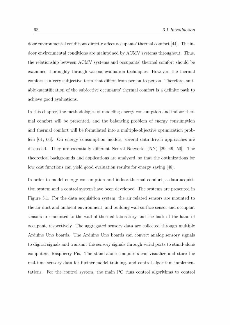
68 3.1 Introduction
door environmental conditions directly affect occupants’ thermal comfort [44]. The in-
door environmental conditions are maintained by ACMV systems throughout. Thus,
the relationship between ACMV systems and occupants’ thermal comfort should be
examined thoroughly through various evaluation techniques. However, the thermal
comfort is a very subjective term that differs from person to person. Therefore, suit-
able quantification of the subjective occupants’ thermal comfort is a definite path to
achieve good evaluations.
In this chapter, the methodologies of modeling energy consumption and indoor ther-
mal comfort will be presented, and the balancing problem of energy consumption
and thermal comfort will be formulated into a multiple-objective optimization prob-
lem [61, 66]. On energy consumption models, several data-driven approaches are
discussed. They are essentially different Neural Networks (NN) [29, 49, 50]. The
theoretical backgrounds and applications are analyzed, so that the optimizations for
low cost functions can yield good evaluation results for energy saving [48].
In order to model energy consumption and indoor thermal comfort, a data acquisi-
tion system and a control system have been developed. The systems are presented in
Figure 3.1. For the data acquisition system, the air related sensors are mounted to
the air duct and ambient environment, and building wall surface sensor and occupant
sensors are mounted to the wall of thermal laboratory and the back of the hand of
occupant, respectively. The aggregated sensory data are collected through multiple
Arduino Uno boards. The Arduino Uno boards can convert analog sensory signals
to digital signals and transmit the sensory signals through serial ports to stand-alone
computers, Raspberry Pis. The stand-alone computers can visualize and store the
real-time sensory data for further model trainings and control algorithm implemen-
tations. For the control system, the main PC runs control algorithms to control

3.1 Introduction 69
the operations of air-conditioning and mechanical ventilation (ACMV) systems by
signaling the variable frequency drives (VFD) of supply air fan motor, water pump
and compressor. The VFDs drive the corresponding electric appliances by altering
the supply voltage frequency. Since the condenser operates constantly at its rated
operating condition once it starts, it is just controlled by on/off modes.
Air Temperature (Duct) Sensor
Air Velocity (Duct) Sensor
Air Humidity (Duct) Sensor
Air Temperature (Ambient) Sensor
Air Velocity (Ambient) Sensor
Air Humidity (Ambient) Sensor
Surface Temperature Sensor
Skin Temperature Sensor
Arduino Uno
Raspberry Pi 2
Serial Comm
Data AcquisitionData VisualizationData Storage
Aggregate Inputs Signals(Analog and Digital)
Python/LabViewScripts
Main PC
TCP/IP Comm
NI CommunicationInterface
Supply Air Fan Motor
Water Pump
Compressor
Condenser
VFD
VFD
VFD
Data Acquisition System Control System
TCP/IPComm
Figure 3.1: Data Acquisition System and Control System
In the section on constructing the indoor thermal comfort models, two different types
of methodologies are illustrated, namely passive and active approaches. The pas-
sive approaches are mainly based on the studies of P.O. Fanger [6] and many great
successors [44, 68, 82]. The quantifications of thermal comfort are based on physi-
cal laws of heat transfer. The heat transfer can be calculated through environmental
parameters and some occupant parameters. The environmental parameters cover am-
bient air temperature, ambient air velocity, air relative humidity and mean radiant
temperature, while occupant parameters are metabolic rate and clothing insulation

70 3.1 Introduction
factor [6, 98]. The active approaches directly utilize occupants’ physiological param-
eters to predict their indoor thermal sensations [21]. The physiological parameters
consist of hight, weight, gender, age, metabolic rate, exposed skin surface area, skin
temperature, blood pressure, etc [20, 60, 74, 96].
In the section on problem formulation and optimization, the main objective is to
formulate and optimize cost functions or objective functions with goals of enhancing
the performance of ACMV systems and the thermal comfort levels of occupants [8,
22, 28, 30, 47, 55]. Therefore, the objective functions for smart buildings will utilize
the knowledge of energy consumption of ACMV systems and indoor thermal comfort
sensations [4, 15, 18, 24, 27, 36, 58]. Plus, a user-preference coefficient is proposed
for adjusting the objective functions according to different user preferences in real
applications [35, 54, 67]. Different optimization algorithms have been investigated.
There are three categories of algorithms discussed, namely nature-inspired algorithms,
Bayesian optimization and analytical algorithms.
Before model methodologies of energy consumption and thermal comfort, a general
experimental procedure is described. For experiments of evaluating energy consump-
tion of ACMV systems, the operating frequencies of supply air fan motor, compressor
and water pump were tuned and recorded from 30 Hz to 50 Hz. The VFDs are
configured to vary frequencies from 0 Hz to 50 Hz. While the frequencies below 30
Hz are not operable to drive apparatuses in thermal laboratory. The energy con-
sumption of ACMV systems was recorded correspondingly by a power meter. In
addition, the ambient/duct air temperature, ambient/duct air relative humidity and
ambient/duct air velocity were also recorded concurrently in data acquisition sys-
tem. For experiments of evaluating thermal comfort of occupants, the subjects were
asked to follow a standard activity level, either general offices duty (case 1) or lec-

3.1 Introduction 71
ture theatres/conference rooms (case 2). The experiments were carried out for 40
minutes for each experimental subject in thermal laboratory. The first 20 minutes
were cooling experiments (duct air temperature around 18 C), and the second 20
minutes were normal experiments (duct air temperature around 24 C). The occu-
pants were given questionnaires to reflect their thermal comfort sensations every 10
minutes. Throughout the experiments, the environmental parameters (ambient air
temperature, ambient air relative humidity, ambient air velocity and clothing insula-
tion factor) and the physiological parameters (activity level, skin temperature, height
and weight) were concurrently collected in data acquisition system for further data
analysis and modeling.
Since the ACMV systems are set up in Singapore (a tropical country), the experiments
mainly focus on cooling capacity of ACMV systems. The latent cooling load basically
refers to the wet bulb temperature of the building, and the sensible cooling load refers
to the dry bulb temperature of the building. The sensible heat profile of the thermal
laboratory can be calculated as follows:
hs = cpρq∆T (3.1)
where cp is the specific heat of air (1.006 kJ/kgC), ρ is the density of air (1.202
kg/m3), q is the air flow rate (m3/s), ∆T is the temperature difference (C).
The rated RPM of supply air fan motor is 3000 rpm, and the variable frequency drive
(VFD) adjusts the speed of motor by operating frequency linearly, thus the RPM of
motor is between 1800 rpm and 3000 rpm (30 Hz to 50 Hz). The rated air flowrate
is about 640 cfm (0.302 m3/s). According to the thermal laboratory profile during

72 3.1 Introduction
experiments and fan laws, the air flow rate follows the rule below:
qunknownqknown
=V FDunknown
V FDknown
(3.2)
Therefore the air flow rate is between 0.1812 m3/s and 0.302 m3/s. The temperature
of the thermal laboratory varies between 16 C to 24 C, thus the profile of sensible
heat profile is between 1.753 kW and 2.921 kW .
In addition, the latent heat profile of the thermal laboratory can be examined as
follows:
hs = ρqhwedwkg (3.3)
where ρ is the density of air (1.202 kg/m3), q is the air flow rate (m3/s), hwe is the
latent heat evaporation water (generally 2454 kJ/kg at air atmospheric condition,
20 C), dwkg is the humidity ratio difference (kg water/kg dryair), which can be
determined by Mollier diagram presented in Figure 3.2.
According to the experimental conditions, the hwe is selected as 2454 kJ/kg as the
condition is a general air atmospheric pressure (Singapore at sea level). The temper-
ature is cooled from 24 C to 16 C in cooling process, and the specific humidity is
between 0.011 kg water/kg dryair and 0.0067 kg water/kg dryair by checking the
Mollier Diagram. With the range of air flow rate of 0.1812 m3/s and 0.302 m3/s
as calculated above, the latent heat profile is between 2.298 kW and 3.83 kW . The
above calculations demonstrate the sensible and latent heat profiles in the thermal
laboratory.
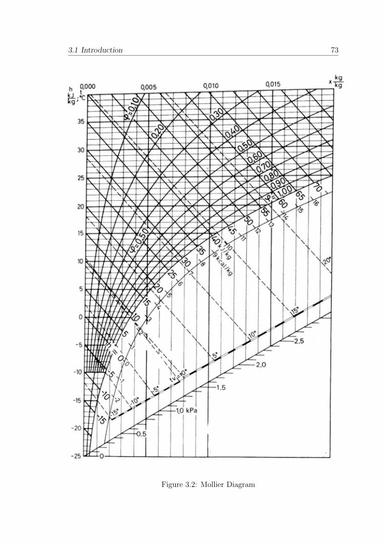
3.1 Introduction 73
Figure 3.2: Mollier Diagram

74 3.2 ACMV Energy Consumption Modeling
3.2 ACMV Energy Consumption Modeling
In this section, the modeling of energy consumption of ACMV systems is presented.
Since the operation conditions of ACMV systems have direct impacts on the energy
consumption as well as the built environment, the correlation study between operation
conditions and energy consumption will offer an important perspective. The operation
data of ACMV systems were collected and recorded through experiments. The ACMV
systems consist of the following units: Air Handling Unit (AHU), Water Chiller Unit
(WCU) and Liquid Dehumidification Unit (LDU) as shown in Figure 3.3. The main
energy consuming apparatuses are supply air fan motor (AHU), compressor (WCU),
water pump (WCU) and condenser (WCU). In this study, the physical systems of
AHU and WCU are illustrated in Figure 3.4, and LDU is presented in Figure 3.5.
In order to operate ACMV systems versatilely, Variable Frequency Drives (VFD)
are applied to supply air fan motor, compressor and water pump. The condenser
is not operated by variable frequency drives (VFD), and it works continuously at
its rated operating condition once started. Traditionally, the energy consumption
of AHU and WCU is examined by power meters measuring currents and voltages,
which make the systems complex and not real-time. Therefore, an ML-based energy
model has been proposed to predict energy consumption in real-time and without
increasing the systems’ complexity. Thus, the whole study are centered around the key
control parameters which are the operating conditions of three components, namely
the supply air fan motor, compressor and water pump. In addition, the models of
supply air fan motor, compressor, water pump, condenser and power meter are listed
in Table 3.1, and the corresponding VFD devices are given in Table 3.2:
The thermal laboratory is the place where experiments were conducted, and it was

3.2 ACMV Energy Consumption Modeling 75
Supply Air Fan
Compressor
Cooling Coils
Evaporator
Water Pump
Condenser
WaterChillerUnit
ElectronicEvaporator
Valve
Air Mixer
OutdoorAir
ReturnedAir
Air Handling Unit
Thermal Laboratory
LiquidDehumidification
Unit
Diffuser
Door
Window
Specifications: 1. Thermal Laboratory Dimensions Length=728 cm, Width=352 cm, Hight=250 cm
2. Duct Dimensions Inner Length=Inner Width=30 cm
3. Diffuser Dimensions Length=116 cm, Width=55 cm
Air-Conditioning and Mechanical Ventilation System
andThermal Laboratory
Water Circulation
Refrigerant Circulation
Figure 3.3: Air-Conditioning and Mechanical Ventilation Systems

76 3.2 ACMV Energy Consumption Modeling
1
2 3
4
5
6 7
8
9
①: AHU-Supply Air Chamber ②: AHU-Cooling Coil ③: AHU-Supply Air Fan Motor ④: WCU-Water Tank ⑤: WCU-Evaporator ⑥: WCU-Water Pump ⑦: WCU-Compressor ⑧: WCU-Condenser ⑨: WCU-Control Panel
Figure 3.4: Air-Handling Unit and Water Chiller Unit
Table 3.1: Electric Appliances of ACMV SystemsAppliance Model Specification
Supply Air Fan Motor TECO INVERTER MOTOR AEHLVS 3P: 0.75 kW (Rated)Compressor BITZER 4CES-6Y-40S 3P: 9.7 kW (Rated)Water Pump SAER ELETTROPOMPE CMP/76 3P: 0.76 kW (Rated)Condenser WOLTER EKH 400-4 1P: 0.47 kW (Rated)Power Meter YOKOGAWA IM CW240E 3P3W/1P2W
Table 3.2: Electric Appliances VFD of ACMV SystemsAppliance Model Specification
Supply Air Fan Motor VFD ABB ACS510 3P: 380 − 480 V , 1.1 − 160 kWCompressor VFD OMRON 3G3MX2-A4055 3P: 400 V , 5.5 kWWater Pump VFD OMRON 3G3MX2-A4040 3P: 400 V , 4.0 kW

3.2 ACMV Energy Consumption Modeling 77
1
2 3
4
5
6 7
8
9 ①: LDU-Supply Air Duct Inlet ②: LDU-Air Fan ③: LDU-Heat Pipes ④: LDU-Water Pump ⑤: LDU-Strong Solution Tank ⑥: LDU-Working Solution Tank ⑦: LDU-Chiller Water ⑧: LDU-Working Solution Tank ⑨: LDU-Supply Air Duct Outlet
Figure 3.5: Liquid Dehumidification Unit

78 3.2 ACMV Energy Consumption Modeling
also one of the main set-ups in the School of Electrical and Electronic Engineering,
Nanyang Technological University, Singapore for studying the performance of ACMV
systems. The thermal laboratory has a dimension of 7.28m× 3.52m× 2.50m (length,
width and height). The thermal laboratory is isolated from the outside environment,
and air-conditioned solely by ACMV systems in the laboratory. Environmental sen-
sors are installed inside the thermal laboratory, and they monitor the environmental
conditions, such as air temperature, air velocity and air relative humidity, etc.
The models of energy consumption of ACMV systems are based on supervised learn-
ing. The model topology of neural networks (NN) is shown in Figure 3.6.
Σ A.F.
𝜽 𝟏
𝜽 𝟐
Σ
A.F.Σ
A.F.
Σ A.F.
+1+1
𝜔1
𝜔2
𝜔3
ΣEnergyConsumption
𝑎1
𝑎2
𝑎3
𝑎𝑘𝑎
𝑥0𝑎0
Input(3-feature)
Output(1-output)(𝑘𝑎-Hidden Neurons)
Figure 3.6: Neural Networks - Energy Consumption
The models are established for monitoring and predicting energy consumption of
ACMV systems. The training of neural networks is based on back-propagation and
convex optimization (basically batch/stochastic gradient descent approaches). The
objective is to minimize the cost function or loss function (i.e. mean squared er-
rors between model results and ground truth results) with respect to feature weights
that will be continuously tuned through back-propagation iterations as mentioned in

3.2 ACMV Energy Consumption Modeling 79
Chapter 2. The parameter tuning process is basically solving a convex optimization
problem. Generally, Lagrange multiplier, Newton’s method and quadratic program-
ming can also be applied to solve this problem in the mathematics point of view.
Based on experimental data, the energy consumption of partially loaded chiller (i.e.
compressor and water pump) is analyzed. The visualization of experimental data is
presented in Figure 3.7. The experimental data shows that the energy consumption of
partially loaded chiller does not always increase with the increase of system operations.
This phenomenon is due to the coupling effects of compressor, water pump and supply
air fan motor.
Compressor Partially Loaded
0.60 0.65 0.70 0.75 0.80 0.85 0.90 0.95 1.00 Water Pump Partially
Loaded
0.600.65
0.700.75
0.800.850.900.951.00
Ener
gy C
onsu
mpt
ion
(kW
)
4.5
5.0
5.5
6.0
6.5
7.0
7.5
8.0
Supply Air Fan 60% Partially LoadedSupply Air Fan 70% Partially LoadedSupply Air Fan 80% Partially LoadedSupply Air Fan 90% Partially LoadedSupply Air Fan 100% Loaded
Figure 3.7: Partially Loaded Chiller Energy Profiles
For the models of energy consumption aforementioned, some key assumptions of these
models are listed as follows:
• The models are merely associated with the operation conditions of ACMV sys-
tems.
• The weather conditions are not incorporated in the models of this study.
• The models are based on an assumption of uniformly distributed environment.

80 3.3 Indoor Thermal Comfort Modeling
3.3 Indoor Thermal Comfort Modeling
In this section, different approaches of evaluating on indoor thermal comfort sensa-
tions are illustrated. These approaches are based on physical laws and data-driven
machine learning techniques. The first group of approaches is largely using envi-
ronmental parameters to train the thermal comfort models. The second group of
approaches is only using physiological parameters to train the thermal comfort mod-
els. The last group of approaches is a hybrid one that can be trained by both en-
vironmental and physiological parameters. In this thesis, only the first and second
groups are discussed in details. To be consistent throughout the thesis, the approach-
es largely based on environmental parameters are called passive approaches, while
the approaches based on physiological parameters are called active approaches.
Figure 3.8: Thermal Laboratory (Left: Inside, Right: Outside)
The experiments were conducted in the thermal laboratory, located at School of
Electrical and Electronic Engineering, Nanyang Technological University, Singapore.
The views of inside and outside the thermal laboratory are illustrated in Figure 3.8.

3.3 Indoor Thermal Comfort Modeling 81
The experimental transducers are installed and utilized to acquire real time data.
The information of transducers is tabulated in the Table 3.3.
Table 3.3: Experimental TransducersParameter Model Specification
Air Temperature - Duct EE21-FT3B56/T07 Range: 0 − 60 C, ± 0.2 CAir Temperature - Ambient AOSONG AM2302 Range: -40 − 80 C, ± 0.5 CAir Relative Humidity - Duct EE21-FT3B56/T07 Range: 0 − 100 %, ± 2 %Air Relative Humidity - Ambient AOSONG AM2302 Range: 0 − 99.9 %, ± 2-5 %Air Velocity - Duct TSI 8455 Range: 0.125 − 50 m/s, ± 2 %Air Velocity - Ambient TSI 8475 Range: 0.05 − 0.5 m/s, ± 1 %Skin Temperature Exacon D-S18JK Range: 0 − 50 C, ± 0.1 CSurface Temperature PT-1000 RTD Range: -200 − 850 C, ± 0.3 C
For the models of thermal comfort (passive and active approaches) aforementioned,
some key assumptions of these models are listed as follows:
• The environmental parameters (ambient air temperature and ambient air ve-
locity and ambient air humidity) in passive approach are treated as uniformly
distributed for simplifying the models.
• The metabolic rate in passive approach is determined by checking activity-
metabolic rate table.
• The skin temperature in active approach is represented by the skin temperature
of the back of the hand.
• The questionnaires for the occupants are assumed to naturally reflect the subjec-
tive feelings which are not biased by the bulky and messy experimental devices.
The experiments are carried out in the thermal laboratory along with questionnaires
for the occupants. The questionnaire is attached in Figure 3.9. The feedbacks of

82 3.3 Indoor Thermal Comfort Modeling
occupants are treated as ground truths for evaluating and validating the models of
passive and active approaches.
Thermal Comfort Questionnaire
This questionnaire is part of study aiming to evaluate thermal comfort levels of occupant in the
experimental indoor environment. We appreciate your feedback, and keep your feedback
confidential. Please fill up and tick appropriately in the form.
1. Name: Gender: Male Female
2. Age: Height: (m) Weight: (kg)
3. Clothing
Please tick the corresponding wearing as you fill up this questionnaire in the Table 1 below.
If your wearing is not listed in Table 1, please describe in the blank space provided below.
Clothing Description:
4. Activity Level
Please tick the most suitable activity as you fill up this questionnaire.
Seated / Writing, 1 met Typing, 1.1 met
Standing Relaxed, 1.2 met Walking About, 1.7 met
Light Machine Work, 2.2 met Heavy Machine Work, 4 met
5. Thermal Comfort Level
Please tick the most suitable level as you fill up this questionnaire.
+3 Hot +2 Warm +1 Slightly Warm 0 Neutral -1 Slightly Cool -2 Cool -3 Cold
Clothing Description Remark
(Please tick appropriately)
Trousers + Short-sleeve shirt
Trousers + Long-sleeve shirt
Trousers + Long-sleeve shirt + Suit jacket
Trousers + Long-sleeve shirt + Suit jacket + Vest + T-shirt
Trousers + Long-sleeve shirt + Long-sleeve sweater + T-shirt
Knee length skirt + Short-sleeve shirt
Knee length skirt + Long-sleeve shirt
Knee length skirt + Long-sleeve shirt + Long-sleeve sweater
Angle-length skirt + Long-sleeve shirt + Suit jacket
Walking shorts + Short-sleeve shirt
Long-sleeve overalls + T-shirt
Overalls + Long-sleeve shirt + T-shirt
Sweat pants + Sweat shirt
Table 1: Clothing Description
Figure 3.9: Thermal Comfort Questionnaire

3.3 Indoor Thermal Comfort Modeling 83
3.3.1 Passive Approach
In passive approaches, the widely-adopted Predicted Mean Vote (PMV) model has
been implemented as thermal comfort sensation indicators. According to the PMV
model, there are seven parameters to predict thermal comfort sensations, and these
parameters are ambient air temperature, ambient air relative humidity, ambient air
velocity, mean radiant temperature, metabolic rate, clothing insulation and external
mechanical work done.
Table 3.4: Angle Factor CoefficientsState Position Fmax A B C D E
SeatedWall or Window facing person 0.118 1.216 0.169 0.717 0.087 0.052Floor or Ceiling facing person 0.116 1.396 0.13 0.951 0.08 0.055
StandingWall or Window facing person 0.12 1.242 0.167 0.616 0.082 0.051Floor or Ceiling facing person 0.116 1.595 0.128 1.226 0.046 0.044
The parameters of ambient air temperature, ambient air relative humidity and ambi-
ent air velocity can be obtained directly by transferring raw analogue voltage signals
into real physical terms, and they are further logged into database with respect to
corresponding operating conditions of ACMV systems for neural networks modeling.
The mean radiant temperature is defined as uniform temperature of a black imagi-
nary enclosure that leads to same heat loss by radiant of the occupant. There are
two ways to determine this parameter.
The first method uses surface temperatures and angle factors to estimate the mean
radiant temperature [6]. The angle factors are calculated through the occupant states
(i.e. seated or standing) and dimensions of space according to REHVA Guidebook
No.7 [6]. The angle factor coefficients are shown in Table 3.4.

84 3.3 Indoor Thermal Comfort Modeling
The equations of calculating angle factors are presented as follows:
Tmr = 4
√√√√ n∑i=1
Fi · (Tsfi + 273)4 − 273
n∑i=1
Fi = 1
τ(p) = A+B ·(a
c
)(p)
γ(p) = C +D ·(b
c
)(p)
+ E ·(a
c
)(p)
Fi(p) = Fmax ·(
1− exp
(− a
c · τ
)(p)
)·(
1− exp
(− b
c · γ
)(p)
)
Fi =4∑p=1
Fi(p)
(3.4)
According to the dimensions of experimental zone (i.e. thermal laboratory), the
calculation matrix of six surface angle factors are given in Table 3.5 and Table 3.6,
where a, b and c are the corresponding surfaces of the experimental space. Therefore,
the mean radiant temperatures can be calculated correspondingly as Eq. 3.4.
The second method is based on air velocity, globe and air temperatures to estimate
mean radiant temperature. A series of equations estimate the mean radiant temper-

3.3 Indoor Thermal Comfort Modeling 85
Table 3.5: Calculations of Angle Factor (Occupant State: Seated)
Subsu
rface
ab
ca/c
b/c
τγ
Fi(p)
Fi
Left
Wall
11.
761.
93.
640.
4835
160.
5219
781.
2977
140.
7875
550.
0177
86
0.04
9945
21.
761.
93.
640.
4835
160.
5219
781.
2977
140.
7875
550.
0177
863
1.76
0.6
3.64
0.48
3516
0.16
4835
1.29
7714
0.75
6484
0.00
7186
41.
760.
63.
640.
4835
160.
1648
351.
2977
140.
7564
840.
0071
86
Rig
ht
Wall
11.
761.
93.
640.
4835
160.
5219
781.
2977
140.
7875
550.
0177
86
0.04
9945
21.
761.
93.
640.
4835
160.
5219
781.
2977
140.
7875
550.
0177
863
1.76
0.6
3.64
0.48
3516
0.16
4835
1.29
7714
0.75
6484
0.00
7186
41.
760.
63.
640.
4835
160.
1648
351.
2977
140.
7564
840.
0071
86
Fro
nt
Wall
13.
641.
91.
762.
0681
821.
0795
451.
5655
230.
9184
660.
0598
06
0.17
6549
23.
641.
91.
762.
0681
821.
0795
451.
5655
230.
9184
660.
0598
063
3.64
0.6
1.76
2.06
8182
0.34
0909
1.56
5523
0.85
4205
0.02
8469
43.
640.
61.
762.
0681
820.
3409
091.
5655
230.
8542
050.
0284
69
Back
Wall
(Win
dow
@0.6
m)
13.
641.
91.
762.
0681
821.
0795
451.
5655
230.
9184
660.
0598
06
0.17
6549
23.
641.
91.
762.
0681
821.
0795
451.
5655
230.
9184
660.
0598
063
3.64
0.6
1.76
2.06
8182
0.34
0909
1.56
5523
0.85
4205
0.02
8469
43.
640.
61.
762.
0681
820.
3409
091.
5655
230.
8542
050.
0284
69
Ceilin
g
13.
641.
761.
91.
9157
890.
9263
161.
6450
531.
1304
740.
0446
34
0.17
8534
23.
641.
761.
91.
9157
890.
9263
161.
6450
531.
1304
740.
0446
343
3.64
1.76
1.9
1.91
5789
0.92
6316
1.64
5053
1.13
0474
0.04
4634
43.
641.
761.
91.
9157
890.
9263
161.
6450
531.
1304
740.
0446
34
Flo
or
13.
641.
760.
66.
0666
672.
9333
332.
1846
671.
5193
330.
0930
03
0.37
201
23.
641.
760.
66.
0666
672.
9333
332.
1846
671.
5193
330.
0930
033
3.64
1.76
0.6
6.06
6667
2.93
3333
2.18
4667
1.51
9333
0.09
3003
43.
641.
760.
66.
0666
672.
9333
332.
1846
671.
5193
330.
0930
03

86 3.3 Indoor Thermal Comfort Modeling
Table 3.6: Calculations of Angle Factor (Occupant State: Standing)Subsu
rface
ab
ca/c
b/c
τγ
Fi(p)
Fi
Left
Wall
11.
761.
33.
640.
4835
160.
3571
431.
3227
470.
6699
450.
0151
82
0.05
8998
21.
761.
33.
640.
4835
160.
3571
431.
3227
470.
6699
450.
0151
823
1.76
1.2
3.64
0.48
3516
0.32
967
1.32
2747
0.66
7692
0.01
4317
41.
761.
23.
640.
4835
160.
3296
71.
3227
470.
6676
920.
0143
17
Rig
ht
Wall
11.
761.
33.
640.
4835
160.
3571
431.
3227
470.
6699
450.
0151
82
0.05
8998
21.
761.
33.
640.
4835
160.
3571
431.
3227
470.
6699
450.
0151
823
1.76
1.2
3.64
0.48
3516
0.32
967
1.32
2747
0.66
7692
0.01
4317
41.
761.
23.
640.
4835
160.
3296
71.
3227
470.
6676
920.
0143
17
Fro
nt
Wall
13.
641.
31.
762.
0681
820.
7386
361.
5873
860.
7820
450.
0534
06
0.20
8884
23.
641.
31.
762.
0681
820.
7386
361.
5873
860.
7820
450.
0534
063
3.64
1.2
1.76
2.06
8182
0.68
1818
1.58
7386
0.77
7386
0.05
1036
43.
641.
21.
762.
0681
820.
6818
181.
5873
860.
7773
860.
0510
36
Back
Wall
(Win
dow
@0.6
m)
13.
641.
31.
762.
0681
820.
7386
361.
5873
860.
7820
450.
0534
06
0.20
8884
23.
641.
31.
762.
0681
820.
7386
361.
5873
860.
7820
450.
0534
063
3.64
1.2
1.76
2.06
8182
0.68
1818
1.58
7386
0.77
7386
0.05
1036
43.
641.
21.
762.
0681
820.
6818
181.
5873
860.
7773
860.
0510
36
Ceilin
g
13.
641.
761.
32.
81.
3538
461.
9534
1.41
1477
0.05
4484
0.21
7935
23.
641.
761.
32.
81.
3538
461.
9534
1.41
1477
0.05
4484
33.
641.
761.
32.
81.
3538
461.
9534
1.41
1477
0.05
4484
43.
641.
761.
32.
81.
3538
461.
9534
1.41
1477
0.05
4484
Flo
or
13.
641.
761.
23.
0333
331.
4666
671.
9832
671.
4269
330.
0583
58
0.23
3431
23.
641.
761.
23.
0333
331.
4666
671.
9832
671.
4269
330.
0583
583
3.64
1.76
1.2
3.03
3333
1.46
6667
1.98
3267
1.42
6933
0.05
8358
43.
641.
761.
23.
0333
331.
4666
671.
9832
671.
4269
330.
0583
58

3.3 Indoor Thermal Comfort Modeling 87
ature as follows:
Tmr = 4
√(Tg + 273)4 +
hc,ghr· (Tg − Ta)− 273
hr = ε · σ = 0.95× 5.67× 10−8 = 5.38× 10⁻⁸
hc,g =
6.3 · (Va)0.6
D0.4g
, (Forced convection)
1.4 ·(|Tg−Ta|Dg
)0.25
, (Free convection)
(3.5)
Compared with the first method, this method is much easier to estimate the mean
radiant temperature with less measurement costs. However, it has drawbacks since it
does not consider the 3 dimensional conditions in space. Therefore, it also normally
results in larger errors in predictions with respect to the first method.
3.3.2 Active Approach
Many researchers have shown that the skin temperatures have the most correlation
with thermal comfort sensations of occupants. In this study, our proposed approach
directly uses physiological parameters to model thermal comfort sensations of occu-
pants. According to the thermal comfort guidelines of ASHRAE Standard 55 2013,
the comfortable guideline of air temperature is between 19.4 C and 27.8 C, and
the comfortable guideline of air humidity is no more than 65%, and the comfortable
guideline of air velocity is between 0.05 m/s and 0.23 m/s [6]. The questionnaire
also follows the ASHRAE’s standard 7 categories of thermal comfort levels, namely
-3 (cold), -2 (cool), -1 (slightly cool), 0 (neutral comfort), 1 (slightly warm), 2 (warm)
and 3 (hot).

88 3.3 Indoor Thermal Comfort Modeling
The experiments in this study were carried out to examine 20 occupant subjects one-
by-one, and each subject had an monitoring period of 40 minutes. The environmental
parameters, physiological parameters and thermal comfort feedbacks of occupants
were recorded concurrently. During the first 20 minutes (cold scenario), the supply-
air temperature of ACMV systems was set at 16 C with normal ventilations. During
the second 20 minutes (general scenario), the supply-air temperature was switched to
24 C with normal ventilations. Before each experiment starts, the experimental room
had been prepared at the corresponding temperature for half an hour, so that the
room condition was considered as a suitable steady-state for conducting experiments.
The skin temperatures of occupant subjects were recorded every second, and their
gradients were calculated accordingly for training models of thermal comfort. Besides
skin temperature and its gradient, there are other physiological parameters to be ad-
dressed, such as height, weight, gender, etc. These parameters are used to normalize
the recorded skin temperatures and corresponding gradients. Since physiological pa-
rameters of height, weight and clothing factor (Icl) impact on skin temperature from
person to person, a normalization factor is proposed by as follows:
Anorm = (1− Icl) · Adu
Adu = Weight0.425 ×Height0.725 × 0.203
(3.6)
where Adu is the Du Bois’s body surface area.
Hereby the normalized skin temperature is derived as follows for later data analyses

3.4 Problem Formulation and Optimization 89
and modeling:
Tsk,norm =TskAnorm
(3.7)
In addition to the many results showing the significant correlations between the skin
temperature of the back of the hand and thermal comfort sensation, the gradient of
skin temperature is also a promising information that can significantly leads to differ-
ent thermal comfort sensations. Thus, the normalized gradient of skin temperature
is also derived as follows for later data analyses and modeling:
Tsk,grad,norm =∇tTskAnorm
(3.8)
3.4 Problem Formulation and Optimization
In this section, optimization problems are described, and mathematical formulations
of the optimization problems are defined. In this thesis, the optimization problems
basically involve energy efficiency evaluations (EEE) and comfort sensation evalua-
tions (CSE) for smart buildings in Singapore. Furthermore, the energy are mainly
consumed by the centralized air-conditioning and mechanical ventilation (ACMV)
systems. Furthermore, the ACMV systems also control and maintain the guaran-
teed indoor air quality that significantly influences the health and productivity of
occupants. Therefore, the optimization problems are narrowed down to balancing
the energy efficiency of air-conditioning and mechanical ventilation (ACMV) systems
and thermal comfort sensations of occupants.

90 3.4 Problem Formulation and Optimization
The optimization problems are classified as multiple-objective non-linear discrete op-
timizations without the knowledge of analytic mathematical expressions for both
objectives. According to the literature on optimization techniques in Chapter 2, the
nature-inspired algorithms and Bayesian optimizer have better advantages in solving
this type of real application optimizations.
The multiple-objective problems are formulated into two parts. The first part is
energy efficiency evaluation (EEE) of air-conditioning and mechanical ventilation
(ACMV) systems, and the second part is comfort sensation evaluation (CSE) of occu-
pants. For the first part, the EEE is determined by supply-air fan motor, compressor,
water pump and condenser of ACMV systems as formulated in Eq. 3.9:
EEE =4∑i=1
Ei(ωi)
ωi =
(ω1, ω2, ω3, ω4
)T, i = 1, 2, 3 and 4
ω1 = ωsaf , E1 = Esaf
ω2 = ωcomp, E2 = Ecomp
ω3 = ωpump, E3 = Epump
ω4 = ωcond, E4 = Econd
(3.9)
For the second part, the CSE will depend upon the approaches used, so it can be
formulated in Eq. 3.10:
CSEpsv = fpsv(M,W,Q)
CSEatv = fatv(Tsk, Icl, Height,Weight)
(3.10)
With EEE of ACMV systems and CSE of occupants, the optimization problems can

3.4 Problem Formulation and Optimization 91
be established by integrating these two components. Since the components have
different numerical scales, the normalizations of EEE and CSE are required before
formulating the objective functions, and the normalizations are shown in Eq. 3.11:
EEEnorm =EEE − EEEmin
EEEmax − EEEmin
CSEnorm =CSE − CSEmin
CSEmax − CSEmin
(3.11)
The normalized EEE and CSE are further formulated as weighted multiple-objective
functions by introducing a user-preference tuning parameter (λ) as shown in Eq. 3.12:
fobj(·) = λ · EEEnorm + (1− λ) · CSEnorm (3.12)
The optimization algorithms are applied to the formulated objective function in order
to search for the specific optimal solutions. The optimization algorithms were exam-
ined using different algorithms from swarm intelligence to Bayesian. In this thesis, a
novel Augmented Firefly Algorithm (AFA) has been proposed and evaluated. It has
been compared with other optimization algorithms, namely classic Firefly Algorithm
(FA), Bayesian optimization, etc. The pseudo-code of AFA is illustrated in Algorithm
11. The innovations and novelties of the proposed AFA algorithm has already been
discussed in Chapter 1.
The evaluation results of computational complexity of classic FA and AFA are il-
lustrated in Figure 3.10. The evaluations are based on a standard 2D optimization
function, namely four-peak function. Based on the computation time experiments,
AFA outperforms classic FA in both studies of iteration and firefly population.

92 3.4 Problem Formulation and Optimization
Algorithm 11 Augmented Firefly Algorithm
1: Define objective function2: f(x), x = (x1, x2, · · · , xd)T3: Initialize population of n fireflies xi (i = 1, 2, · · · , n)4: Determine light intensity Ii at xi by f(xi)5: while (not reach stopping criteria):6: for i = 1 : n (all n fireflies):7: if (Ii < Imax)
8: xnewi = xoldi + α · γ(
xmax − xoldi
)+ β ·
[(∆B − 1) · s+ 1
]· ε
9: Update new intensity Ii by f(xi)10: else
11: xnewi = xoldi + β ·[(∆B − 1) · s+ 1
]· ε
12: Update new intensity Ii by f(xi)13: endfor i14: endwhile15: Visualize population fireflies and obtain global optimum g∗
16: Stop.
Notes:α ∈ (0, 1]: Distance Coefficientβ ∈ [0, 1]: Randomness Coefficientγ ∈ [0, 1]: Vortex Coefficientε: Uniform Distribution (−1, 1) / Gaussian Distribution N (0, 1)∆B: Maximum Boundary Difference
s =
0, (Small Region Wandering)
1, (Large Region Wandering)

3.4 Problem Formulation and Optimization 93
0 100 200 300 400 500Number of Iterations (Population = 100)
0
2
4
6
8
10
12
Comp
utatio
nal T
ime (
seco
nds)
Classic FAAFA
0 100 200 300 400 500Number of Population (Iteration = 500)
0
50
100
150
200
250
300
Comp
utatio
nal T
ime (
seco
nds)
Classic FAAFA
Figure 3.10: Computational Complexity Analysis

94 3.5 Summary
In the study of iteration, the computation time is within a range of 0.04s to 0.8s
for AFA. While the computation time is between 1.2s and 12s for classic FA. The
computation time of classic FA is more than 10 times that of AFA. In the study of
population, the computation time is within a range of 0.2s to 2.2s for AFA. However,
the computation time varies between 0.4s to 293s for classic FA. The computation
time increases exponentially for classic FA with the increase of population.
3.5 Summary
In this chapter, the methodologies of modeling and optimization are presented for
energy consumption and thermal comfort sensations. First, the data acquisition sys-
tem and control system of air-conditioning and mechanical ventilation (ACMV) are
designed and implemented so as to enable the evaluations of subsequent studies on
energy efficiencies and thermal comfort. Second, the different component units of
ACMV systems are introduced in details. The machine learning models of energy
consumption of ACMV systems are described through the neural networks topolo-
gy. Third, the models of thermal comfort sensation are described through the use of
passive and active approaches and verified with 20 experimental occupants. Fourth,
the optimization formulation is described in details, and the justifications of improve-
ment of classic Firefly Algorithm (FA) to yield the proposed Augmented Firefly Al-
gorithm (AFA) are illustrated and demonstrated through computational complexity
evaluations. In the next two chapters, the optimization evaluations between energy
efficiency evaluations (EEE) and comfort sensation evaluations (CSE) are discussed
using passive and active approaches, respectively.

Chapter 4
Energy Efficiency Evaluation- Using Passive Approaches
4.1 Introduction
The very subjective term of “thermal comfort” could have different “quantifications”
for different environmental conditions and occupants. A significant milestone on its
definition can be dated back to 1970s when Fanger developed a way of quantifying
thermal comfort through environmental and occupant parameters [6]. He derived a
term called “Predicted Mean Vote (PMV)” [26] for evaluating thermal comfort levels
of occupants. Based on the conversion from a subjective term to a quantified term, it
is applicable to evaluate the multiple-objective problem of energy efficiency and indoor
thermal comfort. In this chapter, machine learning modeling and experimental results
are presented for energy efficiency evaluations (EEE) based on passive approaches of
thermal comfort sensation evaluations (CSE).
Table 4.1: Two Scenarios in ExperimentsCase 1 Case 2General Offices Lecture Theatres/Conference RoomsM = 70W/m2 M = 93W/m2
Icl = 0.08Km2/W Icl = 0.1Km2/Wφ = 58% φ = 58%
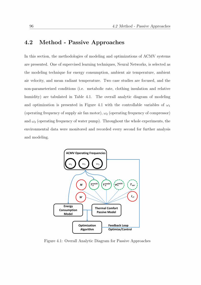
96 4.2 Method - Passive Approaches
4.2 Method - Passive Approaches
In this section, the methodologies of modeling and optimizations of ACMV systems
are presented. One of supervised learning techniques, Neural Networks, is selected as
the modeling technique for energy consumption, ambient air temperature, ambient
air velocity, and mean radiant temperature. Two case studies are focused, and the
non-parameterized conditions (i.e. metabolic rate, clothing insulation and relative
humidity) are tabulated in Table 4.1. The overall analytic diagram of modeling
and optimization is presented in Figure 4.1 with the controllable variables of ω1
(operating frequency of supply air fan motor), ω2 (operating frequency of compressor)
and ω3 (operating frequency of water pump). Throughout the whole experiments, the
environmental data were monitored and recorded every second for further analysis
and modeling.
𝜔1 𝜔2 𝜔3
Energy Consumption
Model
Thermal ComfortPassive Model
𝑻𝒂𝒂𝒎𝒃𝒕 𝑽𝒂
𝒂𝒎𝒃𝒕 𝝋𝒂𝒂𝒎𝒃𝒕 𝑻𝒎𝒓𝑴
𝑾 𝑰𝒄𝒍
ACMV Operating Frequencies
OptimizationAlgorithm
Feedback LoopOptimize/Control
Figure 4.1: Overall Analytic Diagram for Passive Approaches

4.3 Experimental Result and Discussion 97
The external work done (W ) is defaulted as zero. The indoor thermal comfort model
is presented in a series of equations shown in Eq. 4.1 below:
PMV =
(0.303 · e−0.036M + 0.028
)·(M −W −Q
)(4.1)
where
Q = Qdiff +Qevap +Qresp,
Qdiff = 3.05×10−3 ·[5733−6.99 · (M −W )−Pa
]− 1
Icl
[Tcl−35.7+0.028 · (M −W )
],
Qevap = 0.42 · (M −W − 58.15),
Qresp = 1.71× 10⁻⁵ ·M · (5869− Pa) + 0.0014 ·M · (34− Ta),
Tcl = 35.7− 0.028 · (M −W )− Icl
3.96× 10⁻⁸ · fcl ·[(Tcl + 273)4 − (Tmr + 273)4
]+
fcl · hc · (Tcl − Ta)
,
hc = max
2.38 · |Tcl − Ta|1/4
12.1 ·√Va
fcl =
1.00 + 1.29 · Icl, (Icl ≤ 0.078m2K/W.)
1.05 + 0.645 · Icl, (Icl > 0.078m2K/W.)
Pa = 6.11 · φ100· 10
7.5·Ta237.7+Ta .
4.3 Experimental Result and Discussion
Based on numerous experiments, the final models of energy consumption are trained
by assigning 1000 hidden neurons, 500 iterations and 0.1 learning rate; the final models
of ambient air temperature are trained by assigning 500 hidden layer neurons, 500
iterations and 0.1 learning rate; the final models of ambient air velocity are trained
by assigning 500 hidden layer neurons, 500 iterations and 0.01 learning rate. The

98 4.3 Experimental Result and Discussion
transfer function or activation function of neurons is sigmoid function. According to
the training results shown in Figure 4.2, the training costs of models are significantly
reduced as the number of hidden layer neurons and the number of iterations increase.
But the increase of the number of neurons and iterations will lead to time-consuming
training processes. There are trade-offs whenever training processes take place. In
order to perform a trade-off between training time and cost, the training costs of
energy approach zero when the number of hidden neurons reaches 1000, while the
training costs of air temperature and velocity approach zero when the number of
hidden neurons reaches 500. Moreover, the training costs of iterations are almost zero
when the number of iterations is greater than 500. The valleys of training costs on
learning rates are different for energy consumption, air temperature and velocity. It is
better to choose a learning rate within the valley, so that the models can be properly
trained. The valleys of training costs of energy consumption and air temperature
are within a closed interval of [0.01, 0.1]. While the valley of training cost of air
velocity is within a closed interval of [0.001, 0.5]. Based on the above results and
analysis, the final models of energy consumption, air temperature and velocity are
trained according to the aforementioned parameters, and the models are adopted for
further implementation and integration.
The passive approaches of thermal comfort evaluations are based on the simplified
Fanger’s predicted mean vote (PMV) method. Based on the experiments, the e-
valuations and validations of models established with thermal comfort feedbacks of
occupants are presented in Figure 4.3. The PMV model validations show that the
prediction accuracies of PMV in cooling and neutral modes are 70% and 75%, respec-
tively. The feedbacks of occupants are treated as the ground truth data.

4.3 Experimental Result and Discussion 99
100 200 300 400 500 600 700 800 900 10000
0.01
0.02
0.03
0.04
0.05
0.06
0.07
0.08
Number of Hidden Layer Neurons
Cost
Funct
ion (M
ean Sq
uare E
rror)
Evaluations of NN Models with Number of Hidden Layer NeuronsNumber of Iterations=500
Learning Rate=0.1
NN Models of EnergyNN Models of Air TemperatureNN Models of Air Velocity
100 200 300 400 500 600 700 800 900 10000
0.005
0.01
0.015
0.02
0.025
0.03
0.035
0.04
0.045
Number of Iterations
Cost F
unction
(Mean
Squar
ed Err
or)
Evaluations of NN Models with IterationsNumber of Hidden Layer Neurons=1000
Learning Rate=0.1
NN Models of EnergyNN Models of Air TemperatureNN Models of Air Velocity
10-5
10-4
10-3
10-2
10-1
100
0
0.02
0.04
0.06
0.08
0.1
0.12
0.14
0.16
0.18
Learning Rates (Horizontal Axis in Log Scale)
Cost F
unction
(Mean
Squar
ed Err
or)
Evaluations of NN Models with Learning RatesNumber of Hidden Layer Neurons=1000
Number of Iterations=500
NN Models of EnergyNN Models of Air TemperatureNN Models of Air Velocity
Figure 4.2: Evaluations of NN Models on Neuron, Iteration and Learning Rate

100 4.3 Experimental Result and Discussion
2.5 5.0 7.5 10.0 12.5 15.0 17.5 20.0Subject Index
3
2
1
0
1
2
3
Therm
al Co
mfort
Leve
l (t=2
0 min)
PMV Accuracy = 70% Ground TruthPredicted Mean Vote (PMV)
2.5 5.0 7.5 10.0 12.5 15.0 17.5 20.0Subject Index
3
2
1
0
1
2
3
Therm
al Co
mfort
Leve
l (t=4
0 min)
PMV Accuracy = 75% Ground TruthPredicted Mean Vote (PMV)
Figure 4.3: PMV Model Validation
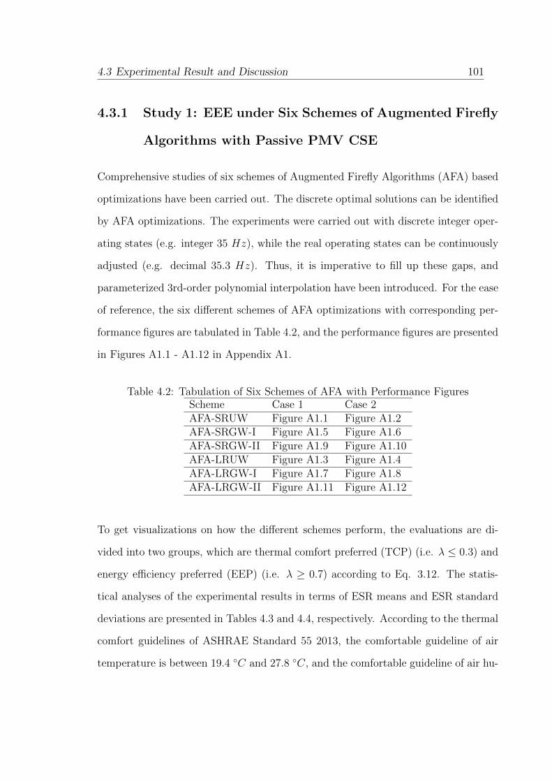
4.3 Experimental Result and Discussion 101
4.3.1 Study 1: EEE under Six Schemes of Augmented Firefly
Algorithms with Passive PMV CSE
Comprehensive studies of six schemes of Augmented Firefly Algorithms (AFA) based
optimizations have been carried out. The discrete optimal solutions can be identified
by AFA optimizations. The experiments were carried out with discrete integer oper-
ating states (e.g. integer 35 Hz), while the real operating states can be continuously
adjusted (e.g. decimal 35.3 Hz). Thus, it is imperative to fill up these gaps, and
parameterized 3rd-order polynomial interpolation have been introduced. For the ease
of reference, the six different schemes of AFA optimizations with corresponding per-
formance figures are tabulated in Table 4.2, and the performance figures are presented
in Figures A1.1 - A1.12 in Appendix A1.
Table 4.2: Tabulation of Six Schemes of AFA with Performance FiguresScheme Case 1 Case 2AFA-SRUW Figure A1.1 Figure A1.2AFA-SRGW-I Figure A1.5 Figure A1.6AFA-SRGW-II Figure A1.9 Figure A1.10AFA-LRUW Figure A1.3 Figure A1.4AFA-LRGW-I Figure A1.7 Figure A1.8AFA-LRGW-II Figure A1.11 Figure A1.12
To get visualizations on how the different schemes perform, the evaluations are di-
vided into two groups, which are thermal comfort preferred (TCP) (i.e. λ ≤ 0.3) and
energy efficiency preferred (EEP) (i.e. λ ≥ 0.7) according to Eq. 3.12. The statis-
tical analyses of the experimental results in terms of ESR means and ESR standard
deviations are presented in Tables 4.3 and 4.4, respectively. According to the thermal
comfort guidelines of ASHRAE Standard 55 2013, the comfortable guideline of air
temperature is between 19.4 C and 27.8 C, and the comfortable guideline of air hu-
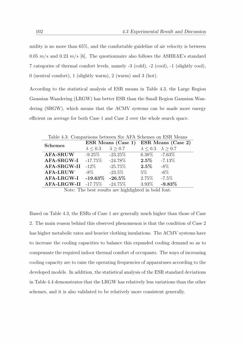
102 4.3 Experimental Result and Discussion
midity is no more than 65%, and the comfortable guideline of air velocity is between
0.05 m/s and 0.23 m/s [6]. The questionnaire also follows the ASHRAE’s standard
7 categories of thermal comfort levels, namely -3 (cold), -2 (cool), -1 (slightly cool),
0 (neutral comfort), 1 (slightly warm), 2 (warm) and 3 (hot).
According to the statistical analysis of ESR means in Table 4.3, the Large Region
Gaussian Wandering (LRGW) has better ESR than the Small Region Gaussian Wan-
dering (SRGW), which means that the ACMV systems can be made more energy
efficient on average for both Case 1 and Case 2 over the whole search space.
Table 4.3: Comparisons between Six AFA Schemes on ESR Means
SchemesESR Means (Case 1) ESR Means (Case 2)λ ≤ 0.3 λ ≥ 0.7 λ ≤ 0.3 λ ≥ 0.7
AFA-SRUW -9.25% -23.25% 6.38% -7.63%AFA-SRGW-I -17.75% -24.78% 2.5% -7.13%AFA-SRGW-II -12% -25.75% 2.5% -8%AFA-LRUW -8% -23.5% 5% -6%AFA-LRGW-I -19.63% -26.5% 2.75% -7.5%AFA-LRGW-II -17.75% -24.75% 3.93% -9.83%
Note: The best results are highlighted in bold font.
Based on Table 4.3, the ESRs of Case 1 are generally much higher than those of Case
2. The main reason behind this observed phenomenon is that the condition of Case 2
has higher metabolic rates and heavier clothing insulations. The ACMV systems have
to increase the cooling capacities to balance this expanded cooling demand so as to
compensate the required indoor thermal comfort of occupants. The ways of increasing
cooling capacity are to raise the operating frequencies of apparatuses according to the
developed models. In addition, the statistical analysis of the ESR standard deviations
in Table 4.4 demonstrates that the LRGW has relatively less variations than the other
schemes, and it is also validated to be relatively more consistent generally.

4.3 Experimental Result and Discussion 103
The reason for good consistency of LRGW is due to its ability to locate the global
optimal solutions instead of the local optimal solutions obtained from SRGW. There-
fore, the results of LRGW are relatively more consistent than those of SRGW. Based
on the experimental results of six different schemes of AFA, we can draw the following
conclusions.
Table 4.4: Comparisons between Six AFA Schemes on ESR Standard Deviations
SchemesESR Std Dev (Case 1) ESR Std Dev (Case 2)λ ≤ 0.3 λ ≥ 0.7 λ ≤ 0.3 λ ≥ 0.7
AFA-SRUW 0.0350 0.0096 0.0382 0.0125AFA-SRGW-I 0.0222 0.0022 0.0342 0.0144AFA-SRGW-II 0.0440 0.0126 0.0311 0.0091AFA-LRUW 0.0337 0.0100 0.0220 0.0071AFA-LRGW-I 0.0189 0.0041 0.0377 0.0000AFA-LRGW-II 0.0104 0.0029 0.0761 0.0379
Note: The best results are highlighted in bold font.
First, Large-Region Wandering (LRW) performs slightly better than Small-Region
Wandering (SRW) based on the continuous regression optimal solutions in Case 1
and Case 2.
Second, Gaussian distribution Wandering (GW) presents better solutions than Unifor-
m distribution Wandering (UW) based on the continuous regression optimal solutions
in Case 1 and Case 2. The Gaussian distribution examines two settings in this study,
namely (µ = 0, σ = 0.1) and (µ = 0, σ = 1), whereas the Uniform distribution only
covers a range of (−0.5,+0.5).
Third, the experimental results show that the Gaussian distribution with σ = 0.1
provides better solutions than the Gaussian distribution with σ = 1. Given the
experimental results, the average maximum potential Energy Saving Rates (ESRs)
are identified at about -26.5% in Case 1 and -9.83% in Case 2, respectively.
104 4.3 Experimental Result and Discussion
Given the three points highlighted above, it is clear that the proposed Large-Region
Gaussian Wandering (LRGW) scheme could effectively achieve a better strategy for
energy efficiency improvement while maintaining satisfactory indoor thermal comfort
conditions in buildings. Besides the technical conclusions drawn, the practical oper-
ations of ACMV systems can also be guided by the real-time optimal solutions on
site (i.e. operating frequencies feedbacks from AFA optimization solutions) obtained
by the proposed models and optimization schemes of AFA. In this way, buildings
can perform more energy efficient and environmental-friendly, while maintaining the
indoor conditions in pre-defined comfort zones. Besides the aforementioned, there are
several limitations that should be noted:
• The thermal laboratory is located in a tropical country. Therefore, the ACMV
systems only provide the cooling capacity, which is not a general Heating and
Ventilation Air-Conditioning (HVAC) system for all four seasons.
• There is an assumption that the rooms in the buildings are identical for the
purpose of experimental simplicity. However, in real applications, each room
is different according to its facing, location inside the building and many other
factors. Therefore, there is a need for room classifications if we aim to compre-
hensively improve the energy efficiency of the whole building.
4.3.2 Study 2: EEE under Classic Firefly Algorithm and
Augmented Firefly Algorithm with Passive PMV CSE
The experimental results from classic FA and AFA optimizations are presented in
Figures A2.1 - A2.6 in Appendix A2, and the experimental results are based on the
well-trained models defined from the previous section. According to the experimental

4.3 Experimental Result and Discussion 105
results, the AFA optimizations generally present better results than the classic FA
optimizations for both Case 1 and Case 2 when the weight coefficient (λ) increases
from 0 to 1. The trend of energy consumption has been shown to decrease when
weight coefficient (λ) increases from 0 to 1. One should note that the discrete actual
optimized results are plotted and based on the experimental data-driven models,
however, the continuing regression results are interpolated and based on the discrete
actual optimized results shown from Figure A2.1 to Figure A2.6 in details.
Moreover, the indoor thermal comfort is also optimized via classic FA and AFA
optimization algorithms for Case 1 and Case 2. The experimental results are presented
in Figure A2.3 and A2.4. The trend of indoor thermal comfort has been shown to
approach the neutral standard when the weight coefficient (λ) decreases from 1 to 0.
On the Energy Saving Rate (ESR) evaluations, the benchmarks of the energy con-
sumption of the ACMV is followed at a median operating points. The ESR exper-
imental results are presented in Figure A2.5 and Figure A2.6. The results of AFA
optimization are better than those of classic FA optimization in both Case 1 and
Case 2. In Case 1, the ESRs of classic FA and AFA optimizations are within intervals
[−25%,−16%] and [−24%,−17%] respectively (λ = 1) among all different genera-
tions at the maximum level of capability as shown in Figure A2.5. In Case 2, the
ESRs of classic FA and AFA optimizations are within intervals [−30%,−18%] and
[−31%,−18%] respectively (λ = 1) among all different generations at the maximum
level of capability as shown in Figure A2.6. The negative values of intervals mean
that the ACMV system operates at a condition of energy efficiency with respect to
median operating conditions.
Based on the experimental evaluations on the optimization algorithms of classic FA
and AFA, the AFA is more efficient in comparison to classic FA. Since the complexity
106 4.3 Experimental Result and Discussion
of FA is O(n2) as shown in classic FA pseudo-code (Algorithm 8) and the complexity
of AFA is O(n) as shown in AFA pseudo-code (Algorithm 11), the accuracy of AFA
is not only better than that of classic FA, but also the computational complexity of
AFA is far less than that of classic FA especially for large population cases.
Based on the results in Figure A2.5 and A2.6, the maximum prediction of potential
ESR can be -30% and -31% via the AFA optimizations for Case 1 and Case 2 while
maintaining indoor thermal comfort in the pre-defined comfort zone.
In this study, there are some limitations to be noted. First, there are limitations in
the experimental results carried on in the laboratory. Since the ACMV system was
uniquely designed and isolated from the school ACMV systems, the experimental
results are limited for the laboratory so far, but the concept can be generally applied.
Second, the experimental results are limited for equator climate regions, since the
experiments were carried out in Singapore, a tropical season country. Third, the
conceptual aim of this study is to optimize the whole buildings’ air and ventilation
controlled by ACMV systems. However, there is a presumption that every single room
is identical for simplicity purpose. Therefore, there are zones-dividing techniques
required for more comprehensively optimizing buildings’ efficiency, which could also
be future study areas as well.
4.3.3 Study 3: EEE under Bayesian Optimization and Aug-
mented Firefly Algorithm with Passive PMV CSE
The experiments were carried out under different initial sizes of samples from 10 to 50.
Due to the constraints of operating conditions of ACMV systems, the boundaries of
operating conditions are set as 50 and 30 for upper and lower boundaries respectively.

4.3 Experimental Result and Discussion 107
AFA optimization is based on computational weight and distance learnings according
to randomly distributed population. The pseudo-code is illustrated in Algorithm 11.
The experimental parameters are presented in Table 4.5 and Table 4.6. The experi-
ments were carried out under different initial sizes of samples ranging from 10 to 50.
Due to the constraints of operating conditions of ACMV systems, the boundaries of
operating conditions are set as 50 and 30 for the upper and lower boundaries. Gaus-
sian distributions of randomness are selected due to better performances of earlier
studies [94].
Table 4.5: Experimental Parameters of Bayesian Gaussian Process OptimizationParameter Sample Boundary θhValue 10/20/30/40/50 50/30 1
Table 4.6: Experimental Parameters of Sparse Augmented Firefly AlgorithmsParameter Sample Boundary α β γ εValue 10/20/30/40/50 50/30 0.6 0.3 0.6 Gaussian (0, 1)
Following the application of the methodologies mentioned in the previous section,
the experimental results of Bayesian Gaussian Process Optimization (BGPO) and
Augmented Firefly Algorithm (AFA) optimization are shown in Figures A3.1 - A3.12
in Appendix A3. Both BGPO and AFA statistical analyses are tabulated in Table
A3.1 - A3.3 in Appendix A3. Based on the statistical analyses, there are two groups
for each of the two cases as Table 4.1 shows. The groups are classified by λ values.
The thermal comfort preferred (TCP) group is classified as λ ≤ 0.3. In addition, for
λ ≥ 0.7, the group is classified as energy efficiency preferred (EEP) group. Comparing
Table A3.1 and A3.2, BGPO generally outperforms AFA in terms of searching for
more optimal solutions, since the means of Energy Saving Rate (ESR) are around -
21% and -10% for BGPO and AFA respectively for both Case 1 and Case 2. However,

108 4.3 Experimental Result and Discussion
AFA is better than BGPO in terms of consistency, and the standard deviations of
ESR are around 0.02 and 0.006 for BGPO and AFA respectively. The increment of
sample sizes improves searching precision and consistency as presented in Table A3.1
and A3.2. As seen in Table A3.3, the evaluations at a sample size of 50 reveals that
AFA is superior to BGPO in terms of consistency. Moreover, BGPO searches more
optimal solutions of ESR than AFA on Case 1 and Case 2. However, AFA locates
more precise solutions of PMV than BGPO on Case 1 and Case 2. Furthermore,
the ESR and PMV results of Case 1 are more optimal than those of Case 2, due to
different environmental resistance to ACMV systems.
Based on the experimental results and analyses of BGPO and AFA above, we can
draw the following conclusions.
First, BGPO outperforms AFA in terms of Energy Saving Rate (ESR) in EEP group.
BGPO has an ESR of -21% for Case 1 and Case 2 in EEP group, while AFA has an
ESR of -10% for Case 1 and Case 2 in EEP group. As the figures presented, BGPO can
perform more energy-saving than AFA does on average. Generally, the experimental
laboratory consumes 73.741 kWh per day for office hours. In terms of economical
performances of these two methodologies, the Singapore Energy Market Authority
announced that the electricity costs 21.56 cents per kWh, and it results in a saving
of about S$1219.1 annually (equivalently 15% of total energy saving according to the
current situation) for such single experimental room compared to general operation
conditions without optimization algorithms applied. If all the rooms in the building
were governed by the methodology, the electricity tariff could be significantly reduced
and demonstrate a large number of economical benefits.
Second, AFA not only surpasses BGPO in terms of indoor thermal comfort (i.e. PMV
index), but also in solution consistency in TCP group. The standard deviation of

4.4 Summary 109
BGPO is around 0.02 for Case 1 and Case 2. While the standard deviation of AFA is
about 0.006 for Case 1 and Case 2. BGPO and AFA have PMV indices of 0.0087 and
0.0008 respectively for Case 1 with a sample size of 50. Similarly, BGPO and AFA
have PMV indices at 0.3463 and 0.1524 respectively for Case 2 with a sample size of
50. As shown in the experimental results, although both of BGPO and AFA have
located the PMV indices within the pre-defined comfort zone, AFA can locate around
10 times and 2 times better than BGPO does for Case 1 and Case 2 respectively.
Third, the improvements of ESR and PMV can be achieved by both BGPO and AFA
with incremental sample sizes. The optimization results in Case 1 are slightly better
than those in Case 2, due to different physiological parameters of the experimental
occupant. The activity level and clothing factor in Case 1 are significantly lower than
those in Case 2. Thus, the cooling demand in Case 2 is higher than that in Case 1,
and the ACMV systems do more work to meet the cooling demand in Case 2.
4.4 Summary
In this chapter, the energy efficiency evaluations (EEE) based on three study topics
have been presented. The EEE is evaluated under passive approaches of comfort
sensation evaluations (CSE) from environmental parameters. The validity and effec-
tiveness of the proposed modeling and optimization algorithms have been validated
under various comparative studies of different schemes and methods. Several limi-
tations in these studies can be summarized as follows: (1) the thermal laboratory
is located in Singapore, so the ACMV systems only provide cooling capacity; (2)
different rooms in buildings are normally different in terms of dimensions, solar ra-
diations, positions and so forth. The experiments were however carried out under
the assumption of identical room for different cases in our study due to limitations

110 4.4 Summary
of experimental platforms and for the purpose of simplicity. However, suitable room
classification techniques can be developed for more comprehensive optimization of
buildings’ efficiency; (3) The indoor comfort actually consists of more than just ther-
mal comfort, and there are luminous comfort and air quality as well. In this study,
the lighting is always provided due to the situation of the thermal laboratory inside
the ACMV laboratory of the School of Electrical and Electronic Engineering. In ad-
dition, since there is only one occupant in this thermal laboratory during each round
of experiment, the air quality (mainly CO2) was always within the acceptable range
while experiments were conducted. Therefore, luminous comfort and air quality of
the experimental room are not in the scope of this thesis, only indoor thermal comfort
has been investigated. In the next chapter, the experimental results of EEE evaluated
with CSE using active approaches will be discussed in details.

Chapter 5
Energy Efficiency Evaluation- Using Active Approaches
5.1 Introduction
Currently, there are many studies on thermal comfort evaluations with active ap-
proaches. In the study of Zhang et al. [96], the thermal sensations of occupants were
discussed on the mean skin temperature of 22 body locations. However, the approach
was developed for an automobile setting, which could not be adopted into real build-
ing environments. Moreover, the approach had high measurement costs, and many
measurements were also intrusive to occupants. In the study of Takada et al. [74],
a mathematical expression of regression model was proposed. The model was built
upon mean skin temperature of 7 body locations. Xiong et al.’s study of thermal sen-
sations of occupants were analyzed from 7 locations of body skin temperature during
transient processes of ambient air temperature [83]. Similarly, Liu et al. proposed a
method of thermal comfort evaluation based on mean skin temperature of 10 body
skin locations in sleeping mode [52]. Due to the constraints of Liu’s work in sleeping
mode, the skin temperature ranges were limited.
Sim et al. [71] analyzed the skin temperature of 4 skin locations near the hand.
The study showed good results, but the validation of models was limited by small

112 5.1 Introduction
sample sizes. The studies mentioned above are basically intrusive to occupants when
measuring those temperatures and they may not be feasible for real applications. In
our earlier studies, the thermal comfort sensations of occupants were evaluated and
modeled by different approaches [17, 90, 91, 93, 94]. The overall analytic diagram of
modeling and optimization is presented in Figure 5.1 with the controllable variables,
such as ω1 (operating frequency of supply air fan motor), ω2 (operating frequency of
compressor) and ω3 (operating frequency of water pump).
𝜔1 𝜔2 𝜔3
Energy Consumption
Model
Thermal ComfortActive Model
Height
ACMV Operating Frequencies
OptimizationAlgorithm
Feedback LoopOptimize/Control
Weight Tsk GenderIcl
Figure 5.1: Overall Analytic Diagram for Active Approaches
In this study, a novel algorithm is proposed to improve Operating State (OS) of
ACMV systems. It is integrated with the models of Predictive Thermal State (PTS)
shown in Figure 5.2 and Figure 5.3. The input of PTS model is physiological pa-

5.1 Introduction 113
rameters of occupants, such as height, weight, clothing and skin temperature. The
output of PTS model is the thermal state of occupant, such as -1 (cool discomfort),
0 (neutral comfort) and 1 (warm discomfort). Considering ASHRAE Standard, the
cool discomfort (-1) is equivalent to -3 and -2 (PMV), and the neutral comfort is
equivalent to -1, 0 and +1 (PMV), and the warm discomfort is equivalent to +2 and
+3 (PMV). The training features are selected as normalized skin temperature and
normalized skin temperature gradient. The training processes are back-propagation
with batch/stochastic gradient descent method.
OccupantPhysiologicalParameters
𝐻𝑒𝑖𝑔ℎ𝑡𝑊𝑒𝑖𝑔ℎ𝑡
𝐼𝑐𝑙
NormalizationFactor
𝑇𝑠𝑘𝑇𝑠𝑘_𝑔𝑟𝑎𝑑
𝑇𝑠𝑘_𝑛𝑜𝑟𝑚𝑇𝑠𝑘_𝑔𝑟𝑎𝑑_𝑛𝑜𝑟𝑚
𝐴𝑛𝑜𝑟𝑚NN
ModelsThermal State(−1,0, +1)
Inputs Output
Figure 5.2: Predictive Thermal State (PTS) Models
PTSModel
Ph
ysio
logi
cal
Para
met
ers
. . .
(-1,0,+1)
ACMVOS
Model
Previous OS
( , )
Current OS
( , )
Figure 5.3: Overall Analytical Diagram (t(k) → t(k+1))
The OS algorithm of ACMV systems alternates OS considering thermal comfort levels
114 5.2 Method - Active Approaches
of occupants in real time, and the overall analytical diagram of this study is shown
in Figure 5.3. The proposed PTS model in this study is trained by neural networks.
The approach is non-intrusive by only using one spot of skin temperature located at
the back of the hand. It could be more feasible for real applications.
5.2 Method - Active Approaches
In this section, methodologies of this study will be illustrated in details. First, PTS
models are adopted and described. Second, OS algorithm of ACMV systems is pro-
posed. Third, the energy consumption of ACMV systems embedded with ACMV OS
algorithm is evaluated by three cases.
The PTS model shown in Figure 5.2 has been presented in details in our earlier
studies [17] and [93], and the PTS model is adopted and applied. The inputs of PTS
model are physiological parameters of occupants, and the models are trained by skin
temperature. The PTS model then provides predictive thermal states of occupants
based on the measurements. The skin temperature (Tsk) was recorded every second,
therefore an extended feature “gradient of skin temperature (Tsk grad)” can be easily
calculated. The proposed normalization factor of Tsk and Tsk grad is governed by Eq.
2.44. In the ACMV OS algorithm, the ACMV systems acquire and alternate OS
every Tsampling, and a modification factor in temperature is noted as ∆T (i.e. 0.1 C).
This problem can be formulated as a Markov Decision Process (MDP). Actions are
taken only on the basis of previous states. The pseudo-code of ACMV OS algorithm is
illustrated in Algorithm 12. This algorithm has two inputs, which are results of PTS
models and Previous Operating State (POS), and the output is Current Operating
State (COS).
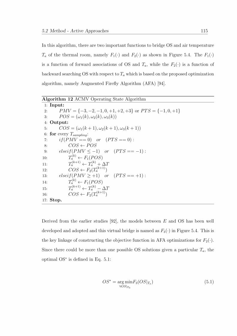
5.2 Method - Active Approaches 115
In this algorithm, there are two important functions to bridge OS and air temperature
Ta of the thermal room, namely F1(·) and F2(·) as shown in Figure 5.4. The F1(·)
is a function of forward associations of OS and Ta, while the F2(·) is a function of
backward searching OS with respect to Ta which is based on the proposed optimization
algorithm, namely Augmented Firefly Algorithm (AFA) [94].
Algorithm 12 ACMV Operating State Algorithm1: Input:2: PMV = −3,−2,−1, 0,+1,+2,+3 or PTS = −1, 0,+13: POS = (ω1(k), ω2(k), ω3(k))4: Output:5: COS = (ω1(k + 1), ω2(k + 1), ω3(k + 1))6: for every Tsampling:7: if(PMV == 0) or (PTS == 0) :8: COS ← POS9: elseif(PMV ≤ −1) or (PTS == −1) :
10: T(k)a ← F1(POS)
11: T(k+1)a ← T
(k)a + ∆T
12: COS ← F2(T(k+1)a )
13: elseif(PMV ≥ +1) or (PTS == +1) :
14: T(k)a ← F1(POS)
15: T(k+1)a ← T
(k)a −∆T
16: COS ← F2(T(k+1)a )
17: Stop.
Derived from the earlier studies [92], the models between E and OS has been well
developed and adopted and this virtual bridge is named as F3(·) in Figure 5.4. This is
the key linkage of constructing the objective function in AFA optimizations for F2(·).
Since there could be more than one possible OS solutions given a particular Ta, the
optimal OS∗ is defined in Eq. 5.1:
OS∗ = arg min∀OS|Ta
F3(OS|Ta) (5.1)

116 5.3 Experimental Result and Discussion
The ACMV systems with ACMV OS algorithm can adjust OS responsively with
respect to thermal comfort levels of occupants in real-time, therefore it could intel-
ligently improve the energy efficiency of ACMV systems while taking the thermal
comfort of occupants into considerations.
𝜔1
𝜔2
𝜔3
𝑇𝑎
𝐹1(∙)
𝐹2(∙)
𝐸
ML Models
𝐹3(∙)
OS
Figure 5.4: Illustrations of Functions F1,F2 and F3
5.3 Experimental Result and Discussion
In this section, the experimental results of air-conditioning and mechanical ventilation
(ACMV) systems are evaluated and the corresponding discussions are presented. The
essential hardware parts of ACMV systems cannot be updated since manufactured.
However, the performance of ACMV systems has been enhanced by the software parts,
namely the proposed models and algorithms in this study. The experimental results
with active approaches are elaborated in this section for energy efficiency evaluations
(EEE) with k-means methods and neural networks modeling methods on comfort
sensation evaluations (CSE).
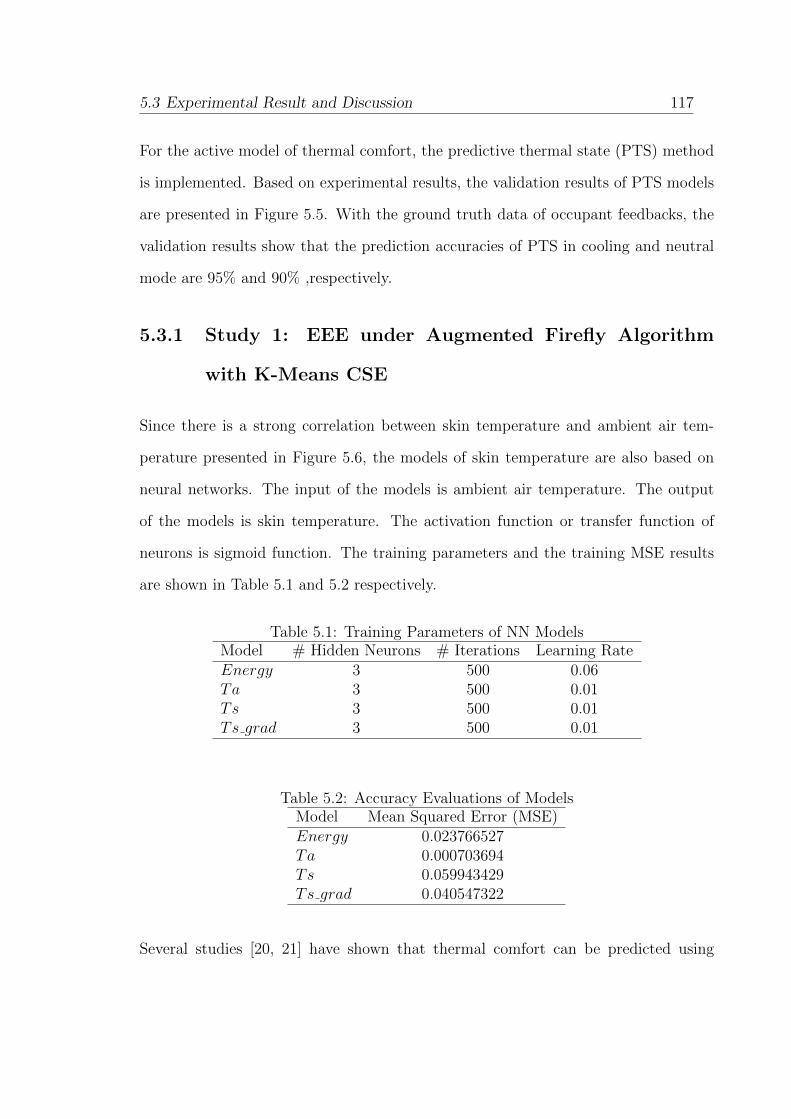
5.3 Experimental Result and Discussion 117
For the active model of thermal comfort, the predictive thermal state (PTS) method
is implemented. Based on experimental results, the validation results of PTS models
are presented in Figure 5.5. With the ground truth data of occupant feedbacks, the
validation results show that the prediction accuracies of PTS in cooling and neutral
mode are 95% and 90% ,respectively.
5.3.1 Study 1: EEE under Augmented Firefly Algorithm
with K-Means CSE
Since there is a strong correlation between skin temperature and ambient air tem-
perature presented in Figure 5.6, the models of skin temperature are also based on
neural networks. The input of the models is ambient air temperature. The output
of the models is skin temperature. The activation function or transfer function of
neurons is sigmoid function. The training parameters and the training MSE results
are shown in Table 5.1 and 5.2 respectively.
Table 5.1: Training Parameters of NN ModelsModel # Hidden Neurons # Iterations Learning RateEnergy 3 500 0.06Ta 3 500 0.01Ts 3 500 0.01Ts grad 3 500 0.01
Table 5.2: Accuracy Evaluations of ModelsModel Mean Squared Error (MSE)Energy 0.023766527Ta 0.000703694Ts 0.059943429Ts grad 0.040547322
Several studies [20, 21] have shown that thermal comfort can be predicted using

118 5.3 Experimental Result and Discussion
2.5 5.0 7.5 10.0 12.5 15.0 17.5 20.0Subject Index
3
2
1
0
1
2
3
Ther
mal
Com
fort
Leve
l (t=
20 m
in)
PTS Accuracy = 95%
Comfort Zone Upper Boundary
Comfort Zone Lower Boundary
Ground Truth (PTS Discomfort Prediction)Ground Truth (PTS Comfort Prediction)
2.5 5.0 7.5 10.0 12.5 15.0 17.5 20.0Subject Index
3
2
1
0
1
2
3
Ther
mal
Com
fort
Leve
l (t=
40 m
in)
PTS Accuracy = 90%
Comfort Zone Upper Boundary
Comfort Zone Lower Boundary
Ground Truth (PTS Discomfort Prediction)Ground Truth (PTS Comfort Prediction)
Figure 5.5: PTS Model Validation

5.3 Experimental Result and Discussion 119
peripheral skin temperature as they are strongly correlated. Moreover, the ambient
air temperature and skin temperature are also strongly correlated as Figure 5.6 shows.
We suggest a new approach for the prediction based on k-means clustering.
20.5 21 21.5 22 22.5 23 23.5 24 24.5 25
29.5
30
30.5
31
31.5
Air temperature (°C)
Ski
n te
mpe
ratu
re ( °
C)
R2 = 0.98
Pearson's correlation = 0.96
Figure 5.6: Correlations between Air Temperature and Skin Temperature
The k-means clustering works by dividing the observations into k distinct cluster-
s depending on target variable, and assigning new observations to the cluster with
shortest Euclidean distance from the cluster centroid. In our study, the thermal com-
fort model inputs are vectors of skin temperature and skin temperature gradient and
the model output is a scalar thermal comfort state, namely “Discomfort (1)” and
“Comfort (0)”. Thus, k=2 clusters for the two states have been employed, and the
optimization problem can be formulated as follows:

120 5.3 Experimental Result and Discussion
Let,
g(ω)
=E(ω) · TC(Ts[Ta(ω)], Ts grad[Ta(ω), Ts(Ta(ω))])
(5.2)
Then,
Problem : ω∗ = argmin∀ω
(g(ω))
Subject to : 30 ≤ ωi∀i≤ 50
g(ω) 6= 0
(5.3)
The energy saving ratio (ESR) is defined as follows:
ESR(ω∗) =E(ω∗)− E(ωbench)
E(ωbench)× 100% (5.4)
where
ω∗ is the optimal operating conditions from AFA optimization algorithm;
ωbench is the nominal benchmark operating conditions of ACMV systems (i.e. ωbench=[40, 40, 40]T );
E(ω) is the energy consumption NN model;
Ta(ω) is the air temperature NN model;
Ts(Ta) is the skin temperature NN model;
Ts grad(Ta, Ts) is the skin temperature gradient NN model; and
TC(Ts, Ts grad) is the thermal comfort k-means model.
Since the previous studies on Augmented Firefly Algorithm (AFA) show better opti-
mization results under identical conditions (i.e. same models and environment) [90],
the AFA is chosen as the optimization algorithm for solving this formulated problem.
The optimization algorithm is previously presented in Algorithm 11. The comparisons

5.3 Experimental Result and Discussion 121
between uniform and Gaussian distribution randomness are presented in Figure 5.7
and Figure 5.8. As the results show, the optimal solutions can be obtained through
larger number of population, and fewer iterations are required when the number of
population is large enough. In comparisons, the results of uniform distribution are
more consistent than those of Gaussian distribution for larger number of population.
It is vice versa for small number of population.
The energy efficiency improvements are presented in Figure 5.9. According to the
results, the optimizations with uniform distribution randomness are more consistent
with larger population, whereas the optimizations with Gaussian distribution ran-
domness are more consistent with smaller population. The trend of ESR is generally
decreasing with the increase of population, and the ESR is generally below -21% (i.e.
improving energy efficiency by 21% and more compared with benchmark operating
conditions).
The results of the k-means approach applied to thermal comfort model are presented
in Figure 5.10. The centroids (Ts, Ts grad) for the Discomfort(1) and Comfort (0)
states are found to be (30.0878, -0.0789) and (32.8751, 0.1358) respectively. The
mean prediction accuracy is found to be 90%. It is to be noted that thermal comfort
states have been predicted with even 100% accuracy for many subjects. Based on the
experimental results, some key conclusions are drawn as follows:
• The skin temperature of occupants has strong correlations with ambient air
temperature, and the highest R2 value can be 0.98.
• The predictions of thermal comfort states can be non-intrusively and feasibly
achieved by measuring skin temperature of occupants with a time interval. The
use of skin temperature and its gradient as features can model thermal comfort

122 5.3 Experimental Result and Discussion
101
102
103
4.62
4.63
4.64
4.65
4.66
4.67
4.68
4.69
4.7
4.71
4.72
Number of fireflies in optimizations (in log scale)
Ene
rgy
Con
sum
ptio
n (in
kW
)
α=0.3α=0.6α=0.9
101
102
103
4.55
4.6
4.65
4.7
4.75
4.8
Number of fireflies in optimizations (in log scale)
Ene
rgy
Con
sum
ptio
n (in
kW
)
α=0.3α=0.6α=0.9
Figure 5.7: Energy Consumption Comparisons: Uniform (Upper) Distribution Ran-domness and Gaussian (Lower) Distribution Randomness

5.3 Experimental Result and Discussion 123
101
102
103
100
101
102
103
104
105
Number of fireflies in optimizations (in log scale)
Num
ber o
f ite
ratio
ns (i
n lo
g sc
ale)
α=0.3α=0.6α=0.9
101
102
103
100
101
102
103
104
Number of fireflies in optimizations (in log scale)
Num
ber o
f ite
ratio
ns (i
n lo
g sc
ale)
α=0.3α=0.6α=0.9
Figure 5.8: Iterations Comparisons: Uniform (Upper) Distribution Randomness andGaussian (Lower) Distribution Randomness

124 5.3 Experimental Result and Discussion
101
102
103
-0.238
-0.236
-0.234
-0.232
-0.23
-0.228
-0.226
-0.224
-0.222
-0.22
Number of fireflies in optimizations (in log scale)
Ene
rgy
Sav
ing
Rat
io (E
SR
)
α=0.3α=0.6α=0.9
101
102
103
-0.25
-0.245
-0.24
-0.235
-0.23
-0.225
-0.22
-0.215
-0.21
-0.205
Number of fireflies in optimizations (in log scale)
Ene
rgy
Sav
ing
Rat
io (E
SR
)
α=0.3α=0.6α=0.9
Figure 5.9: Energy Saving Ratio Comparisons: Uniform (Upper) Distribution Ran-domness and Gaussian (Lower) Distribution Randomness

5.3 Experimental Result and Discussion 125
28 29 30 31 32 33 34 35-1.5
-1
-0.5
0
0.5
1
1.5
2
Skin temperature (°C)
Ski
n te
mpe
ratu
re g
radi
ent (°C
/5m
ins)
Cluster Assignments and Centroids
Comfort ClusterDiscomfort ClusterCentroids
1 2 3 4 5 6 7 8 9 1 0 1 1 1 2 1 3 1 4 1 5 1 6 1 7 1 8 1 9 2 0
7 0
8 0
9 0
1 0 0
Therm
al Co
mfort
Accu
racy (
%)
S u b j e c t s
m e a n a c c u r a c y = 9 0 %
Figure 5.10: Results of K-Means Approach

126 5.3 Experimental Result and Discussion
states with accuracy of as high as 90% on average with k-means approach.
• According to the AFA optimization results, the energy efficiency can be im-
proved by at least 21% when compared with the benchmark operating condi-
tions. Furthermore, the number of iterations decreases when the number of
population increases, and more optimal solutions can be obtained as the num-
ber of population increases as well. In general, the Gaussian distribution is
more consistent than uniform distribution.
5.3.2 Study 2: EEE under Augmented Firefly Algorithm
with Neural Networks CSE
Table 5.3: Physiological Parameters of OccupantOccupant Height (cm) Weight (kg) Icl(clo)Case 1
174 600.67
Case 2 0.42Case 3 0.76
The thermal states of 3 individual cases are illustrated in Table 5.3 and Figure 5.13.
The thermal states of occupants are defined into 3 categories of feelings in this s-
tudy: cool discomfort (-1), neutral comfort (0) and warm discomfort (+1). The skin
temperature of occupants was monitored from 8am to 8pm for 3 consecutive days
(a full-day experiment for each case). From the data of skin temperature, Predic-
tive Thermal State (PTS) model generated the thermal states of these 3 mutually
exclusive cases. The PTS models, which are based on different training features, are
evaluated. The validation results of prediction accuracy are presented in Figure 5.11
and Figure 5.12.
By considering gender differences, the developed PTS models have the best accuracies

5.3 Experimental Result and Discussion 127
Mal
eFe
mal
e0
0.1
0.2
0.3
0.4
0.5
0.6
0.7
0.8
0.91
Prediction Accuracy of NN Models (1-Feature)
Ts Ts,g
rad
Ts,n
orm
Ts,g
rad,
norm
Mal
eFe
mal
e0
0.1
0.2
0.3
0.4
0.5
0.6
0.7
0.8
0.91
Prediction Accuracy of NN Models (2-Feature)
Ts ,
Ts,g
rad
Ts ,
Ts,n
orm
Ts ,
Ts,g
rad,
norm
Ts,g
rad
, Ts,
norm
Ts,g
rad
, Ts,
grad
,nor
m
Ts,n
orm
, Ts
,gra
d,no
rm
Mal
eFe
mal
e0
0.1
0.2
0.3
0.4
0.5
0.6
0.7
0.8
0.91
Prediction Accuracy of NN Models (3-Feature)
Ts ,
Ts,g
rad
, Ts,
norm
Ts ,
Ts,g
rad
, Ts,
grad
,nor
m
Ts ,
Ts,n
orm
, Ts
,gra
d,no
rm
Ts,g
rad
, Ts,
norm
, Ts
,gra
d,no
rm
Mal
eFe
mal
e0
0.1
0.2
0.3
0.4
0.5
0.6
0.7
0.8
0.91
Prediction Accuracy of NN Models (4-Feature)
Ts ,
Ts,g
rad
, Ts,
norm
, Ts
,gra
d,no
rm
Fig
ure
5.11
:P
redic
tion
Acc
ura
cyof
NN
-bas
edP
TS
Model
s(I
tera
tion
=30
000,
Lea
rnin
gR
ate=
0.1)

128 5.3 Experimental Result and Discussion
Male
Female
0
0.1
0.2
0.3
0.4
0.5
0.6
0.7
0.8
0.9 1
Prediction Accuracy of NN Models (1-Feature)
TsTs,grad
Ts,norm
Ts,grad,norm
Male
Female
0
0.1
0.2
0.3
0.4
0.5
0.6
0.7
0.8
0.9 1
Prediction Accuracy of NN Models (2-Feature)
Ts , Ts,grad
Ts , Ts,norm
Ts , Ts,grad,norm
Ts,grad , Ts,norm
Ts,grad , Ts,grad,norm
Ts,norm , Ts,grad,norm
Male
Female
0
0.1
0.2
0.3
0.4
0.5
0.6
0.7
0.8
0.9 1
Prediction Accuracy of NN Models (3-Feature)
Ts , Ts,grad , Ts,norm
Ts , Ts,grad , Ts,grad,norm
Ts , Ts,norm , Ts,grad,norm
Ts,grad , Ts,norm , Ts,grad,norm
Male
Female
0
0.1
0.2
0.3
0.4
0.5
0.6
0.7
0.8
0.9 1
Prediction Accuracy of NN Models (4-Feature)
Ts , Ts,grad , Ts,norm , Ts,grad,norm
Figu
re5.12:
Pred
ictionA
ccuracy
ofN
N-b
asedP
TS
Models
(Iteration=
100000,L
earnin
gR
ate=0.6)

5.3 Experimental Result and Discussion 129
of 96% and 98% for male and female respectively through normalized datasets of skin
temperatures. The training parameters are selected as follows (male/female): (1)
number of neurons is 5/5; (2) number of iterations is 30000/100000; (3) learning
rate is 0.1/0.6; (4) regularization factor is 0.01/0.01; (5) transfer function is sigmoid
function; (6) standard Gaussian is used for data normalization. The PTS models
are adopted from 4-feature models due to the best performances. Augmented firefly
algorithms (AFA) are applied to obtain optimal solutions of operating states (OS) for
feed-backing ACMV systems.
8 10 12 14 16 18 20
Time (hours) in A Day
-1
0
1
Ther
mal
Sta
te
Case 1
Case 2
Case 3
Figure 5.13: Thermal States of 3 Cases in A Day (Tsampling = 10 mins)
Given PTS models of occupants, the ACMV systems can operate intelligently with the
help of this pre-knowledge. The results of a typical sampling time (i.e. Tsampling = 10
mins) are illustrated in Figure 5.14 and the results of accumulated energy consump-
tion are presented in Figure 5.15 for 3 different cases. The results of PTS models
with different sampling time are shown in Figure 5.15 and Table 5.4.
As the Figure 5.14 and Figure 5.15 show, the energy changes of both cases took
place in state transitions throughout the whole day. However, the significant changes
130 5.3 Experimental Result and Discussion
of prediction (Tsampling = 5 mins) did not occur at the most demanding period
of time (i.e. 14 hours or 2pm). The mis-prediction of PTS model is due to fast
sampling, and the occupants had not stabilized yet that cannot be interpreted as
correct information. For Tsampling ≥ 15 mins, the tracking sharpness of occupants’
thermal states was heavily reduced due to long sampling period. The long sampling
period leads to a linear growth in energy consumption throughout the whole day.
The energy consumed is tabulated in Table 5.4 for 3 mutually exclusive cases of full-
day experiments with different Tsampling from 8am to 8pm as ACMV systems operate.
Compared with general operating states, the ACMV systems could be more energy
efficient with PTS information incorporated. The improvement of this experimen-
tal room could save around 10 kWh per day (Tsampling = 10 mins) or about 2.552
Singapore dollars per day without compromising the tracking sharpness of occupants
between state changes. The longer time of Tsampling could improve the energy efficien-
cy of ACMV systems better. However, the systems can be lagging due to the slow
responses of occupant thermal states that lead to uncomfortable sensations between
state transitions.
Clearly, the ACMV systems can be more energy efficient when there are PTS models
involved. Generally, the energy could be reduced by about 10 kWh (around 13.5%
of total daily energy consumption) daily according to the scope of this study in the
laboratory. Moreover, the optimal sampling time (Tsampling) of ACMV OS algorithm
can be set as 10 mins due to its significant changing in OS without losing sharpness
of tracking the occupant thermal states. For Tsampling < 10 mins, the issue is that
the thermal states of occupant are not stabilized due to fast sampling, which leads to
wrong predictions of thermal states. The wrong prediction may or may not cost more
energy, but it does definitely reflect wrong information of occupants to the ACMV

5.3 Experimental Result and Discussion 131
6 8 10 12 14 16 18 20 22
Time (hours) in A Day
-10
0
10
20
30
40
50
60
70
80
Ene
rgy
Con
sum
ptio
n (k
Wh)
in A
Day
Energy without PTS
Energy with PTS (NN Based)-Case 1
Energy with PTS (NN Based)-Case 2
Energy with PTS (NN Based)-Case 3
Figure 5.14: Energy Consumption in A Day (Tsampling = 10 mins)
5 10 15 20 25 30
Sampling Time (mins)
54
56
58
60
62
64
66
68
70
72
74
Ene
rgy
Con
sum
ptio
n in
A D
ay (k
Wh)
No PTS Model (Baseline)NN-Based Case 1
NN-Based Case 2
NN-Based Case 3
Figure 5.15: Energy Consumption in A Day

132 5.3 Experimental Result and Discussion
Table 5.4: Energy Consumption in A Day
Case - Tsampling Baseline PTS (NN Based)Case 1-5 mins 73.741 60.994 (17.29%)Case 2-5 mins 73.741 55.862 (24.25%)Case 3-5 mins 73.741 57.732 (21.71%)Case 1-10 mins 73.741 63.808 (13.47%)Case 2-10 mins 73.741 62.015 (15.90%)Case 3-10 mins 73.741 64.574 (12.43%)Case 1-15 mins 73.741 55.497 (24.74%)Case 2-15 mins 73.741 54.930 (25.51%)Case 3-15 mins 73.741 57.549 (21.96%)Case 1-20 mins 73.741 55.324 (24.98%)Case 2-20 mins 73.741 56.275 (23.69%)Case 3-20 mins 73.741 56.618 (23.22%)Case 1-25 mins 73.741 55.481 (24.76%)Case 2-25 mins 73.741 55.721 (24.44%)Case 3-25 mins 73.741 58.011 (21.33%)Case 1-30 mins 73.741 55.001 (25.41%)Case 2-30 mins 73.741 55.102 (25.28%)Case 3-30 mins 73.741 57.818 (21.59%)
Notes: Values in brackets are the percentages of energy saving. Other values are inthe unit of kWh.

5.4 Summary 133
systems, which make the environment uncomfortable. For Tsampling ≥ 10 mins, the
sharpness of tracking occupant thermal states can be heavily impacted. The ACMV
systems cannot response in time for actions and hence result in lagging performance
(i.e. the plots of energy consumption are more linear).
5.4 Summary
In this chapter, the energy efficiency evaluations (EEE) are examined by two case
studies. The EEE is evaluated under active approaches of comfort sensation evalua-
tions (CSE) from occupant physiological parameters. The validity and effectiveness
of the proposed modeling and optimization algorithms have been tested and validated
under two topics. Several limitations should be considered: (1) The ACMV Oper-
ating State (OS) algorithm is only based on the same single occupant in these case
studies to mimic different occupant conditions. If there are more than one occupants
in the laboratory, then the PTS model cannot predict the overall thermal states of
all occupants. This would be the future direction of study. (2) The PTS model was
developed for the Singapore local climate (i.e. tropical climate). Therefore, the PTS
model may have limitations of applications on other climatic conditions. The PTS
model should be re-trained with new datasets on newly-applied climatic conditions.


Chapter 6
Conclusion
In this chapter, the author shall draw some insightful conclusions based on the pro-
posed algorithms and experimental studies in this thesis. Some limitations of the
studies are also summarized. Several interesting and relevant extensions and prob-
lems are highlighted for future research.
6.1 Conclusion
In this study, the promising concepts of artificial intelligence (AI) and internet of
things (IoT) have been integrated and validated in the platform of air-conditioning
and mechanical ventilation (ACMV) systems in Nanyang Technological University,
Singapore. The key contributions and main conclusions of this PhD study on smart
and energy efficient buildings can be summarized below.
Key Contributions:
1. The author developed a systematic data acquisition system for acquiring
environmental parameters of thermal laboratory and physiological parameters
of occupants by Dell laptop (Windows 10 operating system), Matlab 2017a,
Python 3.6, Arduino Uno, Raspberry Pi 2 (Debian operating system) and re-
spective sensors (i.e. air temperature, air velocity, air relative humidity, human

136 6.1 Conclusion
skin temperature and surface temperature sensors). The author also developed
a machine learning control system of ACMV systems to facilitate carrying
out experiments in the laboratory platform.
2. The author developed and validated machine learning data-driven models of
energy consumption of ACMV systems, and data-driven models of ther-
mal comfort of occupants (i.e. passive and active approaches). The proposed
passive approaches largely use environmental parameters, while the proposed
active approaches use physiological parameters. For both passive and active
approaches, an important normalization process has been proposed in this s-
tudy for data pre-processing. The models have been validated by experimental
results in the thermal laboratory and they show significant improvements on
prediction accuracy with 70% and 90% for passive and active approaches,
respectively.
3. The author formulated the aggregated models of energy consumption and mod-
els of thermal comfort sensations by proposing a user-preference tuning pa-
rameter. The tuning parameter has been verified to increase the flexibility
of operations in ACMV systems on different customer demand profiles in real
applications.
4. The author developed and validated the proposed algorithms by applying them
on the formulated objective problems of this study. The author also accom-
plished the implementations and comparisons of algorithms, namely classic
firefly algorithm (FA), newly proposed augmented firefly algorithm (AFA) and
Bayesian algorithms (Bayesian Gaussian processes). The AFA is one of the
key proposed algorithms in this study. Compared with classic FA, the key
modifications of AFA are summarized as follows: (1) reduce the number of

6.1 Conclusion 137
inner for-loops, (2) introduce vortex coefficient, (3) introduce randomness mode
switches, (4) introduce searching mode switches, (5) modify updating equations.
The modifications of (1) and (5) reduce the computational complexity signifi-
cantly, and the modifications of (2)-(4) help to locate high performance solutions
without sub-optima trapping. The experimental results validated that the AFA
followed a linear trend of computational complexity, while the classic FA has an
exponential trend of computational complexity with the increase of population.
Main conclusions:
For passive approaches in comfort sensation evaluations (CSE), the energy efficiency
evaluations (EEE) of different study topics are summarized as follows:
• Data-driven models of energy consumption and environmental parameters
have been developed and examined by supervised learning techniques with back-
propagation and batch gradient descent algorithms.
• Augmented firefly algorithm (AFA) has been proposed, examined and validated
through a experimental platform of ACMV systems on energy efficiency and
thermal comfort sensations.
• Evaluations of classic firefly algorithm (FA) and augmented firefly algorithm
(AFA) show that AFA generally outperforms FA in terms of global optima
searching capability, computational complexity and consistency.
• Evaluations of the six different schemes of AFA show that Large Region and
Gaussian distribution Wandering (LRGW) generally outperforms the other
schemes in the problems of PhD study.
138 6.1 Conclusion
• The best experimental results of AFA optimizations are demonstrated through
thermal laboratory, and the maximum potentials of energy saving are about
-26.5% for Case 1 (general offices) and -9.83% for Case 2 (lecture theatres/
conference rooms).
• The optimal solutions of AFA are more consistent than those of Bayesian Gaus-
sian process optimization (BGPO) at given sample sizes. The maximum po-
tential of energy saving by BGPO and AFA are around -21% and -10%
respectively for Case 1 (general offices) and Case 2 (lecture theatres/ confer-
ence rooms).
For active approaches in comfort sensation evaluations (CSE), the energy efficiency
evaluations (EEE) of different study topics are summarized as follows:
• The prediction of thermal comfort states via k-means approach has been im-
plemented and it is based on features of skin temperature and skin temperature
gradient. The prediction accuracy of differentiation using skin temperature
and its gradient is up to 90%. The experimental results show that the ener-
gy efficiency can be improved by 21% with the predictive models of thermal
comfort sensations.
• The predictive models of thermal comfort states through neural networks
(NN) have been developed and examined. Based on skin temperature, height,
weight, gender and clothing factors, the accuracy of male and female models
can reach up to 96% and 98%, respectively. The optimal sampling time
of ACMV OS algorithm is 10 mins without the issues of system lagging
and sharpness losing for predictive thermal states of occupants, and it reduces
the energy consumption of thermal laboratory by around 10 kWh out of 74

6.2 Limitations 139
kWh per day, namely about saving S$2.55 in current electricity tariff rate of
Singapore (about 13.5% energy reduction).
6.2 Limitations
In this study, there are several limitations that should be highlighted as follows:
• The thermal laboratory is located in tropical Singapore. Therefore, the set-ups
of air-conditioning and mechanical ventilation (ACMV) systems only provide
the cooling capacity without the need for heating capacity, which are not general
heating, ventilation and air-conditioning (HVAC) systems for all multi-season
and multi-geographical situations.
• There is an assumption that the rooms in the buildings are identical for the
purpose of experimental simplicity. However, in real applications, each room is
different from its facing, location inside the building and many other factors.
Therefore, there is a need for room classifications to be incorporated if we aim
to comprehensively improve the energy efficiency of the whole building.
• The ACMV operating state algorithm is only based on a single occupant in
these case studies to mimic different occupant conditions. If there were more
than one occupants in thermal laboratory, then the PTS model may have to
use some other techniques, for instance weighted states for each occupant, so
to integrate the overall thermal state of all of the occupants.

140 6.3 Future Research Directions
6.3 Future Research Directions
Considering the limitations outlined, several future research directions are pointed as
follows:
• The modeling and optimization approaches developed in this thesis can be fur-
ther enhanced. The energy consumption modeling of operating air conditioning
and mechanical ventilation (ACMV) systems can address different geograph-
ic locations that make the models more comprehensive, robust and adaptable.
The optimization can be further investigated under the various factors of en-
ergy efficiency, thermal comfort sensations, air quality, system failure rates,
maintenance costs, etc.
• Indoor zone differentiations and classifications are worthy of further study to
investigate the handling algorithms of different zones. Occupant indoor posi-
tioning is essential under this research. The handling algorithms can utilize the
inputs of occupant positions and zone classifications, so that they can precise-
ly alter the operating conditions of lights, windows, doors and centralized air
conditioning systems smartly.
• Multiple-occupant comfort sensation evaluations should also be future directions
with the incorporation of zone handling algorithms to achieve energy efficient
smart buildings. With the non-intrusive information from the proposed thermal
comfort models, a general zone thermal comfort model can be investigated and
examined for centralized air conditioning systems.

Appendix A1
Comprehensive comparisons of six schemes of sparse Augmented Firefly Algorithms
(AFA) based on passive Predicted Mean Vote (PMV) are examined on energy efficient
evaluations in the figures below. The different schemes are about small/large regions
and Gaussian/uniform wanderings. The algorithms are examined under two cases,
such as general offices (Case 1) and lecture theatres/conference rooms (Case 2).
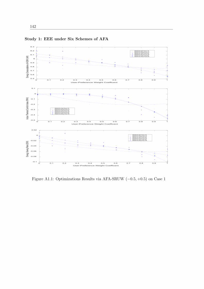
142
Study 1: EEE under Six Schemes of AFA
0 0.1 0.2 0.3 0.4 0.5 0.6 0.7 0.8 0.9 1
User-Preference Weight Coefficent
5.5
5.6
5.7
5.8
5.9
6
6.1
6.2
6.3
Energy
Consum
ptions o
f ACMV
(kW)
NN(AFA)-Opt:Pop=10NN(AFA)-Reg:Pop=10NN(AFA)-Opt:Pop=30NN(AFA)-Reg:Pop=30NN(AFA)-Opt:Pop=50NN(AFA)-Reg:Pop=50
0 0.1 0.2 0.3 0.4 0.5 0.6 0.7 0.8 0.9 1
User-Preference Weight Coefficent
-0.5
-0.4
-0.3
-0.2
-0.1
0
0.1
Indoor T
hermal C
omfort I
ndex (P
MV)
NN(AFA)-Opt:Pop=10NN(AFA)-Reg:Pop=10NN(AFA)-Opt:Pop=30NN(AFA)-Reg:Pop=30NN(AFA)-Opt:Pop=50NN(AFA)-Reg:Pop=50
0 0.1 0.2 0.3 0.4 0.5 0.6 0.7 0.8 0.9 1
User-Preference Weight Coefficent
-0.1
-0.08
-0.06
-0.04
-0.02
0
0.02
Energy
Saving
Rate (E
SR)
NN(AFA)-Opt:Pop=10NN(AFA)-Reg:Pop=10NN(AFA)-Opt:Pop=30NN(AFA)-Reg:Pop=30NN(AFA)-Opt:Pop=50NN(AFA)-Reg:Pop=50
Figure A1.1: Optimizations Results via AFA-SRUW (−0.5,+0.5) on Case 1

143
Study 1: EEE under Six Schemes of AFA
0 0.1 0.2 0.3 0.4 0.5 0.6 0.7 0.8 0.9 1
User-Preference Weight Coefficent
5.6
5.8
6
6.2
6.4
6.6
Energy
Consum
ptions o
f ACMV
(kW)
NN(AFA)-Opt:Pop=10
NN(AFA)-Reg:Pop=10
NN(AFA)-Opt:Pop=30
NN(AFA)-Reg:Pop=30
NN(AFA)-Opt:Pop=50
NN(AFA)-Reg:Pop=50
0 0.1 0.2 0.3 0.4 0.5 0.6 0.7 0.8 0.9 1
User-Preference Weight Coefficent
0.3
0.35
0.4
0.45
0.5
0.55
Indoor T
hermal C
omfort I
ndex (P
MV)
NN(AFA)-Opt:Pop=10
NN(AFA)-Reg:Pop=10
NN(AFA)-Opt:Pop=30
NN(AFA)-Reg:Pop=30
NN(AFA)-Opt:Pop=50
NN(AFA)-Reg:Pop=50
0 0.1 0.2 0.3 0.4 0.5 0.6 0.7 0.8 0.9 1
User-Preference Weight Coefficent
-0.1
-0.08
-0.06
-0.04
-0.02
0
0.02
0.04
0.06
Energy
Saving
Rate (E
SR)
NN(AFA)-Opt:Pop=10NN(AFA)-Reg:Pop=10NN(AFA)-Opt:Pop=30NN(AFA)-Reg:Pop=30NN(AFA)-Opt:Pop=50NN(AFA)-Reg:Pop=50
Figure A1.2: Optimizations Results via AFA-SRUW (−0.5,+0.5) on Case 2

144
Study 1: EEE under Six Schemes of AFA
0 0.1 0.2 0.3 0.4 0.5 0.6 0.7 0.8 0.9 1
User-Preference Weight Coefficent
5.6
5.8
6
6.2
6.4
6.6
Energy
Consum
ptions o
f ACMV
(kW)
NN(AFA)-Opt:Pop=10NN(AFA)-Reg:Pop=10NN(AFA)-Opt:Pop=30NN(AFA)-Reg:Pop=30NN(AFA)-Opt:Pop=50NN(AFA)-Reg:Pop=50
0 0.1 0.2 0.3 0.4 0.5 0.6 0.7 0.8 0.9 1
User-Preference Weight Coefficent
-0.5
-0.4
-0.3
-0.2
-0.1
0
0.1
Indoor T
hermal C
omfort I
ndex (P
MV)
NN(AFA)-Opt:Pop=10NN(AFA)-Reg:Pop=10NN(AFA)-Opt:Pop=30NN(AFA)-Reg:Pop=30NN(AFA)-Opt:Pop=50NN(AFA)-Reg:Pop=50
0 0.1 0.2 0.3 0.4 0.5 0.6 0.7 0.8 0.9 1
User-Preference Weight Coefficent
-0.1
-0.08
-0.06
-0.04
-0.02
0
0.02
0.04
0.06
Energy
Saving
Rate (E
SR)
NN(AFA)-Opt:Pop=10
NN(AFA)-Reg:Pop=10
NN(AFA)-Opt:Pop=30
NN(AFA)-Reg:Pop=30
NN(AFA)-Opt:Pop=50
NN(AFA)-Reg:Pop=50
Figure A1.3: Optimizations Results via AFA-LRUW (−0.5,+0.5) on Case 1

145
Study 1: EEE under Six Schemes of AFA
0 0.1 0.2 0.3 0.4 0.5 0.6 0.7 0.8 0.9 1
User-Preference Weight Coefficent
5.6
5.8
6
6.2
6.4
6.6
Energy
Consum
ptions o
f ACMV
(kW)
NN(AFA)-Opt:Pop=10
NN(AFA)-Reg:Pop=10
NN(AFA)-Opt:Pop=30
NN(AFA)-Reg:Pop=30
NN(AFA)-Opt:Pop=50
NN(AFA)-Reg:Pop=50
0 0.1 0.2 0.3 0.4 0.5 0.6 0.7 0.8 0.9 1
User-Preference Weight Coefficent
0.3
0.35
0.4
0.45
0.5
0.55
Indoor T
hermal C
omfort I
ndex (P
MV)
NN(AFA)-Opt:Pop=10
NN(AFA)-Reg:Pop=10
NN(AFA)-Opt:Pop=30
NN(AFA)-Reg:Pop=30
NN(AFA)-Opt:Pop=50
NN(AFA)-Reg:Pop=50
0 0.1 0.2 0.3 0.4 0.5 0.6 0.7 0.8 0.9 1
User-Preference Weight Coefficent
-0.1
-0.05
0
0.05
0.1
Energy
Saving
Rate (E
SR)
NN(AFA)-Opt:Pop=10
NN(AFA)-Reg:Pop=10
NN(AFA)-Opt:Pop=30
NN(AFA)-Reg:Pop=30
NN(AFA)-Opt:Pop=50
NN(AFA)-Reg:Pop=50
Figure A1.4: Optimizations Results via AFA-LRUW (−0.5,+0.5) on Case 2

146
Study 1: EEE under Six Schemes of AFA
0 0.1 0.2 0.3 0.4 0.5 0.6 0.7 0.8 0.9 1
User-Preference Weight Coefficent
5.6
5.7
5.8
5.9
6
6.1
6.2
Energy
Consum
ptions o
f ACMV
(kW)
NN(AFA)-Opt:Pop=10NN(AFA)-Reg:Pop=10NN(AFA)-Opt:Pop=30NN(AFA)-Reg:Pop=30NN(AFA)-Opt:Pop=50NN(AFA)-Reg:Pop=50
0 0.1 0.2 0.3 0.4 0.5 0.6 0.7 0.8 0.9 1
User-Preference Weight Coefficent
-0.5
-0.4
-0.3
-0.2
-0.1
0
0.1
Indoor T
hermal C
omfort I
ndex (P
MV)
NN(AFA)-Opt:Pop=10NN(AFA)-Reg:Pop=10NN(AFA)-Opt:Pop=30NN(AFA)-Reg:Pop=30NN(AFA)-Opt:Pop=50NN(AFA)-Reg:Pop=50
0 0.1 0.2 0.3 0.4 0.5 0.6 0.7 0.8 0.9 1
User-Preference Weight Coefficent
-0.1
-0.08
-0.06
-0.04
-0.02
0
0.02
Energy
Saving
Rate (E
SR)
NN(AFA)-Opt:Pop=10
NN(AFA)-Reg:Pop=10
NN(AFA)-Opt:Pop=30
NN(AFA)-Reg:Pop=30
NN(AFA)-Opt:Pop=50
NN(AFA)-Reg:Pop=50
Figure A1.5: Optimizations Results via AFA-SRGW-I (µ = 0, σ = 0.1) on Case 1

147
Study 1: EEE under Six Schemes of AFA
0 0.1 0.2 0.3 0.4 0.5 0.6 0.7 0.8 0.9 1
User-Preference Weight Coefficent
5.6
5.8
6
6.2
6.4
6.6
Energy
Consum
ptions o
f ACMV
(kW)
NN(AFA)-Opt:Pop=10NN(AFA)-Reg:Pop=10NN(AFA)-Opt:Pop=30NN(AFA)-Reg:Pop=30NN(AFA)-Opt:Pop=50NN(AFA)-Reg:Pop=50
0 0.1 0.2 0.3 0.4 0.5 0.6 0.7 0.8 0.9 1
User-Preference Weight Coefficent
0.36
0.38
0.4
0.42
0.44
0.46
0.48
0.5
0.52
Indoor T
hermal C
omfort I
ndex (P
MV)
NN(AFA)-Opt:Pop=10
NN(AFA)-Reg:Pop=10
NN(AFA)-Opt:Pop=30
NN(AFA)-Reg:Pop=30
NN(AFA)-Opt:Pop=50
NN(AFA)-Reg:Pop=50
0 0.1 0.2 0.3 0.4 0.5 0.6 0.7 0.8 0.9 1
User-Preference Weight Coefficent
-0.08
-0.06
-0.04
-0.02
0
0.02
0.04
0.06
Energy
Saving
Rate (E
SR)
NN(AFA)-Opt:Pop=10NN(AFA)-Reg:Pop=10NN(AFA)-Opt:Pop=30NN(AFA)-Reg:Pop=30NN(AFA)-Opt:Pop=50NN(AFA)-Reg:Pop=50
Figure A1.6: Optimizations Results via AFA-SRGW-I (µ = 0, σ = 0.1) on Case 2

148
Study 1: EEE under Six Schemes of AFA
0 0.1 0.2 0.3 0.4 0.5 0.6 0.7 0.8 0.9 1
User-Preference Weight Coefficent
5.5
6
6.5
Energy
Consum
ptions o
f ACMV
(kW) NN(AFA)-Opt:Pop=10
NN(AFA)-Reg:Pop=10NN(AFA)-Opt:Pop=30NN(AFA)-Reg:Pop=30NN(AFA)-Opt:Pop=50NN(AFA)-Reg:Pop=50
0 0.1 0.2 0.3 0.4 0.5 0.6 0.7 0.8 0.9 1
User-Preference Weight Coefficent
-0.5
-0.4
-0.3
-0.2
-0.1
0
0.1
Indoor T
hermal C
omfort I
ndex (P
MV)
NN(AFA)-Opt:Pop=10
NN(AFA)-Reg:Pop=10
NN(AFA)-Opt:Pop=30
NN(AFA)-Reg:Pop=30
NN(AFA)-Opt:Pop=50
NN(AFA)-Reg:Pop=50
0 0.1 0.2 0.3 0.4 0.5 0.6 0.7 0.8 0.9 1
User-Preference Weight Coefficent
-0.15
-0.1
-0.05
0
0.05
Energy
Saving
Rate (E
SR)
NN(AFA)-Opt:Pop=10
NN(AFA)-Reg:Pop=10
NN(AFA)-Opt:Pop=30
NN(AFA)-Reg:Pop=30
NN(AFA)-Opt:Pop=50
NN(AFA)-Reg:Pop=50
Figure A1.7: Optimizations Results via AFA-LRGW-I (µ = 0, σ = 0.1) on Case 1
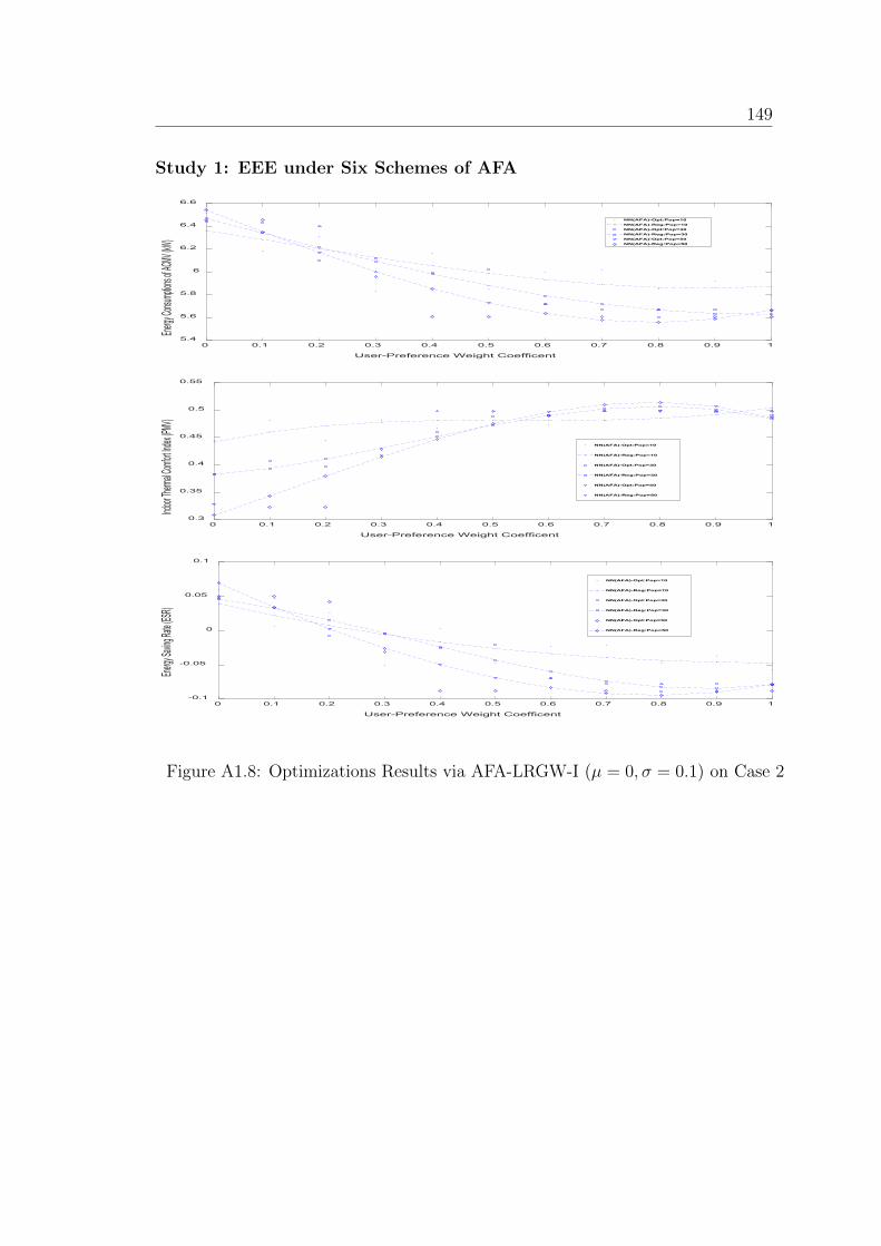
149
Study 1: EEE under Six Schemes of AFA
0 0.1 0.2 0.3 0.4 0.5 0.6 0.7 0.8 0.9 1
User-Preference Weight Coefficent
5.4
5.6
5.8
6
6.2
6.4
6.6
Energy
Consum
ptions o
f ACMV
(kW)
NN(AFA)-Opt:Pop=10NN(AFA)-Reg:Pop=10NN(AFA)-Opt:Pop=30NN(AFA)-Reg:Pop=30NN(AFA)-Opt:Pop=50NN(AFA)-Reg:Pop=50
0 0.1 0.2 0.3 0.4 0.5 0.6 0.7 0.8 0.9 1
User-Preference Weight Coefficent
0.3
0.35
0.4
0.45
0.5
0.55
Indoor T
hermal C
omfort I
ndex (P
MV)
NN(AFA)-Opt:Pop=10
NN(AFA)-Reg:Pop=10
NN(AFA)-Opt:Pop=30
NN(AFA)-Reg:Pop=30
NN(AFA)-Opt:Pop=50
NN(AFA)-Reg:Pop=50
0 0.1 0.2 0.3 0.4 0.5 0.6 0.7 0.8 0.9 1
User-Preference Weight Coefficent
-0.1
-0.05
0
0.05
0.1
Energy
Saving
Rate (E
SR)
NN(AFA)-Opt:Pop=10
NN(AFA)-Reg:Pop=10
NN(AFA)-Opt:Pop=30
NN(AFA)-Reg:Pop=30
NN(AFA)-Opt:Pop=50
NN(AFA)-Reg:Pop=50
Figure A1.8: Optimizations Results via AFA-LRGW-I (µ = 0, σ = 0.1) on Case 2
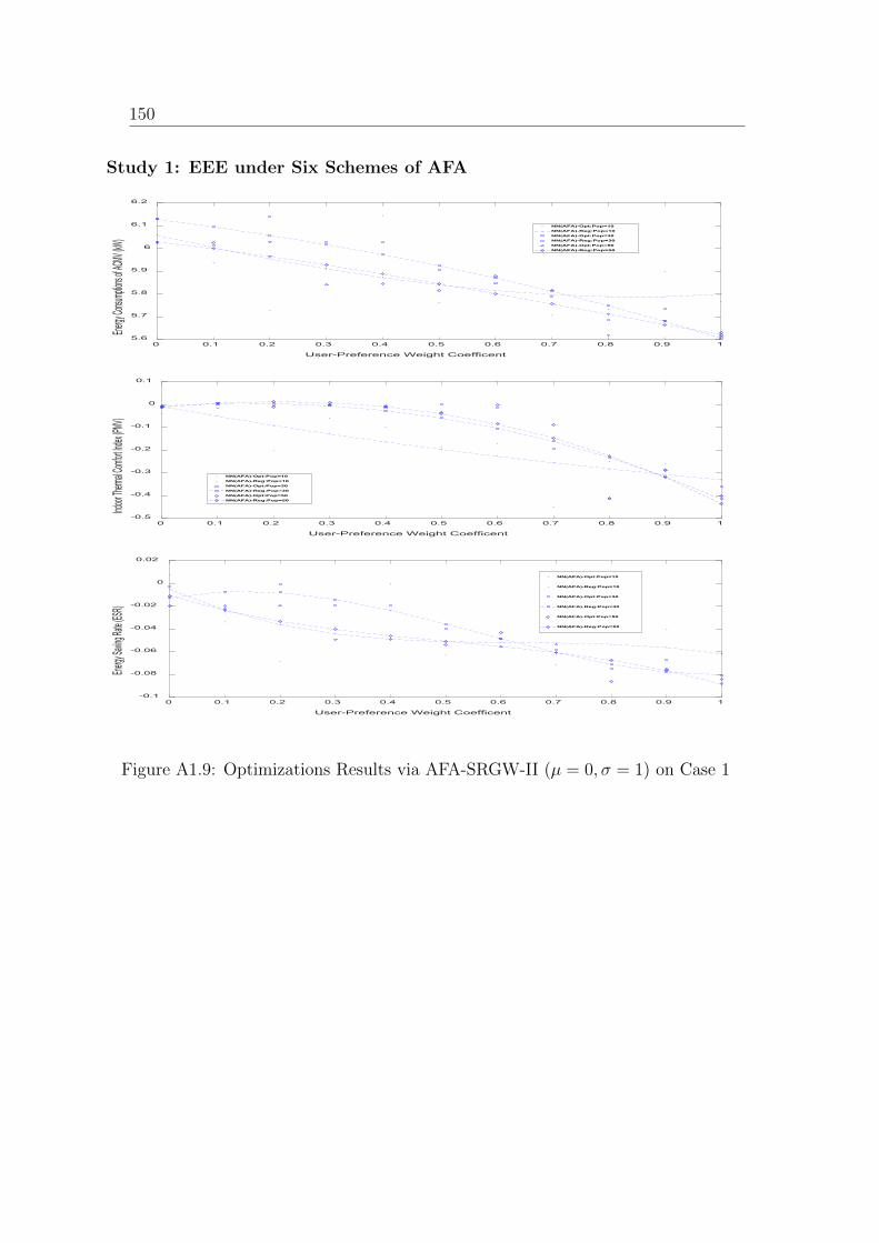
150
Study 1: EEE under Six Schemes of AFA
0 0.1 0.2 0.3 0.4 0.5 0.6 0.7 0.8 0.9 1
User-Preference Weight Coefficent
5.6
5.7
5.8
5.9
6
6.1
6.2
Energy
Consum
ptions o
f ACMV
(kW)
NN(AFA)-Opt:Pop=10NN(AFA)-Reg:Pop=10NN(AFA)-Opt:Pop=30NN(AFA)-Reg:Pop=30NN(AFA)-Opt:Pop=50NN(AFA)-Reg:Pop=50
0 0.1 0.2 0.3 0.4 0.5 0.6 0.7 0.8 0.9 1
User-Preference Weight Coefficent
-0.5
-0.4
-0.3
-0.2
-0.1
0
0.1
Indoor T
hermal C
omfort I
ndex (P
MV)
NN(AFA)-Opt:Pop=10
NN(AFA)-Reg:Pop=10
NN(AFA)-Opt:Pop=30
NN(AFA)-Reg:Pop=30
NN(AFA)-Opt:Pop=50
NN(AFA)-Reg:Pop=50
0 0.1 0.2 0.3 0.4 0.5 0.6 0.7 0.8 0.9 1
User-Preference Weight Coefficent
-0.1
-0.08
-0.06
-0.04
-0.02
0
0.02
Energy
Saving
Rate (E
SR)
NN(AFA)-Opt:Pop=10
NN(AFA)-Reg:Pop=10
NN(AFA)-Opt:Pop=30
NN(AFA)-Reg:Pop=30
NN(AFA)-Opt:Pop=50
NN(AFA)-Reg:Pop=50
Figure A1.9: Optimizations Results via AFA-SRGW-II (µ = 0, σ = 1) on Case 1

151
Study 1: EEE under Six Schemes of AFA
0 0.1 0.2 0.3 0.4 0.5 0.6 0.7 0.8 0.9 1
User-Preference Weight Coefficent
5.4
5.6
5.8
6
6.2
6.4
6.6
Energy
Consum
ptions o
f ACMV
(kW)
NN(AFA)-Opt:Pop=10NN(AFA)-Reg:Pop=10NN(AFA)-Opt:Pop=30NN(AFA)-Reg:Pop=30NN(AFA)-Opt:Pop=50NN(AFA)-Reg:Pop=50
0 0.1 0.2 0.3 0.4 0.5 0.6 0.7 0.8 0.9 1
User-Preference Weight Coefficent
0.3
0.35
0.4
0.45
0.5
0.55
Indoor T
hermal C
omfort I
ndex (P
MV)
NN(AFA)-Opt:Pop=10NN(AFA)-Reg:Pop=10NN(AFA)-Opt:Pop=30NN(AFA)-Reg:Pop=30NN(AFA)-Opt:Pop=50NN(AFA)-Reg:Pop=50
0 0.1 0.2 0.3 0.4 0.5 0.6 0.7 0.8 0.9 1
User-Preference Weight Coefficent
-0.1
-0.05
0
0.05
0.1
Energy
Saving
Rate (E
SR)
NN(AFA)-Opt:Pop=10NN(AFA)-Reg:Pop=10NN(AFA)-Opt:Pop=30NN(AFA)-Reg:Pop=30NN(AFA)-Opt:Pop=50NN(AFA)-Reg:Pop=50
Figure A1.10: Optimizations Results via AFA-SRGW-II (µ = 0, σ = 1) on Case 2

152
Study 1: EEE under Six Schemes of AFA
0 0.1 0.2 0.3 0.4 0.5 0.6 0.7 0.8 0.9 1
User-Preference Weight Coefficent
5.4
5.5
5.6
5.7
5.8
5.9
6
6.1
6.2
Energy
Consum
ptions o
f ACMV
(kW)
NN(AFA)-Opt:Pop=10
NN(AFA)-Reg:Pop=10
NN(AFA)-Opt:Pop=30
NN(AFA)-Reg:Pop=30
NN(AFA)-Opt:Pop=50
NN(AFA)-Reg:Pop=50
0 0.1 0.2 0.3 0.4 0.5 0.6 0.7 0.8 0.9 1
User-Preference Weight Coefficent
-0.6
-0.5
-0.4
-0.3
-0.2
-0.1
0
0.1
Indoor T
hermal C
omfort I
ndex (P
MV)
NN(AFA)-Opt:Pop=10
NN(AFA)-Reg:Pop=10
NN(AFA)-Opt:Pop=30
NN(AFA)-Reg:Pop=30
NN(AFA)-Opt:Pop=50
NN(AFA)-Reg:Pop=50
0 0.1 0.2 0.3 0.4 0.5 0.6 0.7 0.8 0.9 1
User-Preference Weight Coefficent
-0.12
-0.1
-0.08
-0.06
-0.04
-0.02
0
0.02
Energy
Saving
Rate (E
SR)
NN(AFA)-Opt:Pop=10
NN(AFA)-Reg:Pop=10
NN(AFA)-Opt:Pop=30
NN(AFA)-Reg:Pop=30
NN(AFA)-Opt:Pop=50
NN(AFA)-Reg:Pop=50
Figure A1.11: Optimizations Results via AFA-LRGW-II (µ = 0, σ = 1) on Case 1

153
Study 1: EEE under Six Schemes of AFA
0 0.1 0.2 0.3 0.4 0.5 0.6 0.7 0.8 0.9 1
User-Preference Weight Coefficent
5.6
5.8
6
6.2
6.4
6.6
Energy
Consum
ptions o
f ACMV
(kW)
NN(AFA)-Opt:Pop=10NN(AFA)-Reg:Pop=10NN(AFA)-Opt:Pop=30NN(AFA)-Reg:Pop=30NN(AFA)-Opt:Pop=50NN(AFA)-Reg:Pop=50
0 0.1 0.2 0.3 0.4 0.5 0.6 0.7 0.8 0.9 1
User-Preference Weight Coefficent
0.3
0.35
0.4
0.45
0.5
0.55
Indoor T
hermal C
omfort I
ndex (P
MV)
NN(AFA)-Opt:Pop=10
NN(AFA)-Reg:Pop=10
NN(AFA)-Opt:Pop=30
NN(AFA)-Reg:Pop=30
NN(AFA)-Opt:Pop=50
NN(AFA)-Reg:Pop=50
0 0.1 0.2 0.3 0.4 0.5 0.6 0.7 0.8 0.9 1
User-Preference Weight Coefficent
-0.1
-0.08
-0.06
-0.04
-0.02
0
0.02
0.04
0.06
Energy
Saving
Rate (E
SR)
NN(AFA)-Opt:Pop=10NN(AFA)-Reg:Pop=10NN(AFA)-Opt:Pop=30NN(AFA)-Reg:Pop=30NN(AFA)-Opt:Pop=50NN(AFA)-Reg:Pop=50
Figure A1.12: Optimizations Results via AFA-LRGW-II (µ = 0, σ = 1) on Case 2


Appendix A2
Energy efficiency evaluations of classic Firefly Algorithms (FA) and Augmented Fire-
fly Algorithm (AFA) with passive Predicted Mean Vote (PMV) are presented in the
figures below. The algorithms are examined under two cases, such as general offices
(Case 1) and lecture theatres/conference rooms (Case 2).

156
Study 2: EEE under Classic FA and AFA
0 0.1 0.2 0.3 0.4 0.5 0.6 0.7 0.8 0.9 1
User-Preference Weight Coefficent
4.4
4.6
4.8
5
5.2
5.4
5.6
5.8
6
6.2
6.4
Energ
y Con
sump
tions
of AC
MV (k
W)
NN(FA)-Opt:Pop=100
NN(FA)-Reg:Pop=100
NN(FA)-Opt:Pop=50
NN(FA)-Reg:Pop=50
NN(FA)-Opt:Pop=25
NN(FA)-Reg:Pop=25
0 0.1 0.2 0.3 0.4 0.5 0.6 0.7 0.8 0.9 1
User-Preference Weight Coefficent
4.6
4.8
5
5.2
5.4
5.6
5.8
6
6.2
Energ
y Con
sump
tions
of AC
MV (k
W)
NN(AFA)-Opt:Pop=100
NN(AFA)-Reg:Pop=100
NN(AFA)-Opt:Pop=50
NN(AFA)-Reg:Pop=50
NN(AFA)-Opt:Pop=25
NN(AFA)-Reg:Pop=25
Figure A2.1: Sparse FA and AFA Optimizations on Energy Consumption of ACMVSystems (Case 1: Sedentary Activities, e.g. General Offices)

157
Study 2: EEE under Classic FA and AFA
0 0.1 0.2 0.3 0.4 0.5 0.6 0.7 0.8 0.9 14.5
5
5.5
6
6.5
7
7.5
8
Energ
y Con
sump
tions
of AC
MV (k
W)
NN(FA)-Opt:Pop=100
NN(FA)-Reg:Pop=100
NN(FA)-Opt:Pop=50
NN(FA)-Reg:Pop=50
NN(FA)-Opt:Pop=25
NN(FA)-Reg:Pop=25
0 0.1 0.2 0.3 0.4 0.5 0.6 0.7 0.8 0.9 1
User-Preference Weight Coefficent
4.5
5
5.5
6
6.5
7
7.5
Energ
y Con
sump
tions
of AC
MV (k
W)
NN(AFA)-Opt:Pop=100
NN(AFA)-Reg:Pop=100
NN(AFA)-Opt:Pop=50
NN(AFA)-Reg:Pop=50
NN(AFA)-Opt:Pop=25
NN(AFA)-Reg:Pop=25
Figure A2.2: Sparse FA and AFA Optimizations on Energy Consumption of ACMVSystems (Case 2: Light Activities, e.g. Lecture Theatres and Conference Rooms)

158
Study 2: EEE under Classic FA and AFA
0 0.1 0.2 0.3 0.4 0.5 0.6 0.7 0.8 0.9 1
User-Preference Weight Coefficent
0
0.05
0.1
0.15
0.2
0.25
0.3
0.35
0.4
0.45
0.5
Therm
al Co
mfort
Inde
x (PM
V)
NN(FA)-Opt:Pop=100
NN(FA)-Reg:Pop=100
NN(FA)-Opt:Pop=50
NN(FA)-Reg:Pop=50
NN(FA)-Opt:Pop=25
NN(FA)-Reg:Pop=25
0 0.1 0.2 0.3 0.4 0.5 0.6 0.7 0.8 0.9 1
User-Preference Weight Coefficent
0
0.05
0.1
0.15
0.2
0.25
0.3
0.35
0.4
Therm
al Co
mfort
Inde
x (PM
V)
NN(AFA)-Opt:Pop=100
NN(AFA)-Reg:Pop=100
NN(AFA)-Opt:Pop=50
NN(AFA)-Reg:Pop=50
NN(AFA)-Opt:Pop=25
NN(AFA)-Reg:Pop=25
Figure A2.3: Sparse FA and AFA Optimizations on Indoor Thermal Comfort (Case1: Sedentary Activities, e.g. General Offices)

159
Study 2: EEE under Classic FA and AFA
0 0.1 0.2 0.3 0.4 0.5 0.6 0.7 0.8 0.9 1
User-Preference Weight Coefficent
0.3
0.32
0.34
0.36
0.38
0.4
0.42
0.44
0.46
0.48
0.5
Therm
al Co
mfort
Inde
x (PM
V)
NN(FA)-Opt:Pop=100
NN(FA)-Reg:Pop=100
NN(FA)-Opt:Pop=50
NN(FA)-Reg:Pop=50
NN(FA)-Opt:Pop=25
NN(FA)-Reg:Pop=25
0 0.1 0.2 0.3 0.4 0.5 0.6 0.7 0.8 0.9 1
User-Preference Weight Coefficent
0.3
0.32
0.34
0.36
0.38
0.4
0.42
0.44
0.46
0.48
0.5
Therm
al Co
mfort
Inde
x (PM
V)
NN(AFA)-Opt:Pop=100
NN(AFA)-Reg:Pop=100
NN(AFA)-Opt:Pop=50
NN(AFA)-Reg:Pop=50
NN(AFA)-Opt:Pop=25
NN(AFA)-Reg:Pop=25
Figure A2.4: Sparse FA and AFA Optimizations on Indoor Thermal Comfort (Case2: Light Activities, e.g. Lecture Theatres and Conference Rooms)

160
Study 2: EEE under Classic FA and AFA
0 0.1 0.2 0.3 0.4 0.5 0.6 0.7 0.8 0.9 1
User-Preference Weight Coefficent
-0.25
-0.2
-0.15
-0.1
-0.05
0
0.05
Energ
y Sav
ing Ra
te (ES
R)
NN(FA)-Opt:Pop=100
NN(FA)-Reg:Pop=100
NN(FA)-Opt:Pop=50
NN(FA)-Reg:Pop=50
NN(FA)-Opt:Pop=25
NN(FA)-Reg:Pop=25
0 0.1 0.2 0.3 0.4 0.5 0.6 0.7 0.8 0.9 1
User-Preference Weight Coefficent
-0.25
-0.2
-0.15
-0.1
-0.05
0
0.05
Energ
y Sav
ing Ra
te (ES
R)
NN(AFA)-Opt:Pop=100
NN(AFA)-Reg:Pop=100
NN(AFA)-Opt:Pop=50
NN(AFA)-Reg:Pop=50
NN(AFA)-Opt:Pop=25
NN(AFA)-Reg:Pop=25
Figure A2.5: Sparse FA and AFA Optimizations on Energy Saving Rate (ESR) (Case1: Sedentary Activities, e.g. General Offices)

161
Study 2: EEE under Classic FA and AFA
0 0.1 0.2 0.3 0.4 0.5 0.6 0.7 0.8 0.9 1
User-Preference Weight Coefficent
-0.25
-0.2
-0.15
-0.1
-0.05
0
0.05
0.1
0.15
0.2
0.25
Energ
y Sav
ing Ra
te (ES
R)
NN(FA)-Opt:Pop=100
NN(FA)-Reg:Pop=100
NN(FA)-Opt:Pop=50
NN(FA)-Reg:Pop=50
NN(FA)-Opt:Pop=25
NN(FA)-Reg:Pop=25
0 0.1 0.2 0.3 0.4 0.5 0.6 0.7 0.8 0.9 1
User-Preference Weight Coefficent
-0.25
-0.2
-0.15
-0.1
-0.05
0
0.05
0.1
0.15
0.2
0.25
Energ
y Sav
ing Ra
te (ES
R)
NN(AFA)-Opt:Pop=100
NN(AFA)-Reg:Pop=100
NN(AFA)-Opt:Pop=50
NN(AFA)-Reg:Pop=50
NN(AFA)-Opt:Pop=25
NN(AFA)-Reg:Pop=25
Figure A2.6: Sparse FA and AFA Optimizations on Energy Saving Rate (ESR) (Case2: Light Activities, e.g. Lecture Theatres and Conference Rooms)


Appendix A3
Energy efficiency evaluations of Augmented Firefly Algorithm (AFA) and Bayesian
Optimization with passive Predicted Mean Vote (PMV) are presented in the figures
below. The algorithms are examined under two cases, such as general offices (Case
1) and lecture theatres/conference rooms (Case 2).

164
Study 3: EEE under BGPO and AFA
0 0.1 0.2 0.3 0.4 0.5 0.6 0.7 0.8 0.9 14.4
4.6
4.8
5
5.2
5.4
5.6
5.8
6
6.2
6.4
User-Preference Weight Coefficient (λ)
Energy
Consum
ption (k
W)
Initial Sample=10Initial Sample=20Initial Sample=30Initial Sample=40Initial Sample=50
0 0.1 0.2 0.3 0.4 0.5 0.6 0.7 0.8 0.9 14.5
5
5.5
6
User-Preference Weight Coefficient (λ)
Energy
Consum
ption (k
W)
Initial Sample=10Initial Sample=20Initial Sample=30Initial Sample=40Initial Sample=50
Figure A3.1: Energy Consumption BGPO Case 1 - Discrete(Upper) / Regression(Lower)

165
Study 3: EEE under BGPO and AFA
0 0.1 0.2 0.3 0.4 0.5 0.6 0.7 0.8 0.9 1-0.4
-0.35
-0.3
-0.25
-0.2
-0.15
-0.1
-0.05
0
0.05
0.1
User-Preference Weight Coefficient (λ)
Indoor T
hermal C
omfort
(PMV)
Initial Sample=10Initial Sample=20Initial Sample=30Initial Sample=40Initial Sample=50
0 0.1 0.2 0.3 0.4 0.5 0.6 0.7 0.8 0.9 1-0.3
-0.25
-0.2
-0.15
-0.1
-0.05
0
0.05
User-Preference Weight Coefficient (λ)
Indoor T
hermal C
omfort
(PMV)
Initial Sample=10Initial Sample=20Initial Sample=30Initial Sample=40Initial Sample=50
Figure A3.2: Indoor Thermal Comfort BGPO Case 1 - Discrete(Upper) / Regression(Lower)

166
Study 3: EEE under BGPO and AFA
0 0.1 0.2 0.3 0.4 0.5 0.6 0.7 0.8 0.9 1-0.25
-0.2
-0.15
-0.1
-0.05
0
0.05
0.1
User-Preference Weight Coefficient (λ)
Energy
Saving
Rate (E
SR)
Initial Sample=10Initial Sample=20Initial Sample=30Initial Sample=40Initial Sample=50
0 0.1 0.2 0.3 0.4 0.5 0.6 0.7 0.8 0.9 1-0.25
-0.2
-0.15
-0.1
-0.05
0
User-Preference Weight Coefficient (λ)
Energy
Saving
Rate (E
SR)
Initial Sample=10Initial Sample=20Initial Sample=30Initial Sample=40Initial Sample=50
Figure A3.3: Energy Saving Rate BGPO Case 1 - Discrete(Upper) / Regression(Lower)

167
Study 3: EEE under BGPO and AFA
0 0.1 0.2 0.3 0.4 0.5 0.6 0.7 0.8 0.9 14.5
5
5.5
6
6.5
7
7.5
User-Preference Weight Coefficient (λ)
Energy
Consum
ption (k
W)
Initial Sample=10Initial Sample=20Initial Sample=30Initial Sample=40Initial Sample=50
0 0.1 0.2 0.3 0.4 0.5 0.6 0.7 0.8 0.9 14
4.5
5
5.5
6
6.5
7
7.5
User-Preference Weight Coefficient (λ)
Energy
Consum
ption (k
W)
Initial Sample=10Initial Sample=20Initial Sample=30Initial Sample=40Initial Sample=50
Figure A3.4: Energy Consumption BGPO Case 2 - Discrete(Upper) / Regression(Lower)

168
Study 3: EEE under BGPO and AFA
0 0.1 0.2 0.3 0.4 0.5 0.6 0.7 0.8 0.9 1
0.35
0.4
0.45
0.5
0.55
0.6
0.65
0.7
User-Preference Weight Coefficient (λ)
Indoor T
hermal C
omfort
(PMV)
Initial Sample=10Initial Sample=20Initial Sample=30Initial Sample=40Initial Sample=50
0 0.1 0.2 0.3 0.4 0.5 0.6 0.7 0.8 0.9 1
0.35
0.4
0.45
0.5
0.55
0.6
0.65
0.7
User-Preference Weight Coefficient (λ)
Indoor T
hermal C
omfort
(PMV)
Initial Sample=10Initial Sample=20Initial Sample=30Initial Sample=40Initial Sample=50
Figure A3.5: Indoor Thermal Comfort BGPO Case 2 - Discrete(Upper) / Regression(Lower)

169
Study 3: EEE under BGPO and AFA
0 0.1 0.2 0.3 0.4 0.5 0.6 0.7 0.8 0.9 1-0.25
-0.2
-0.15
-0.1
-0.05
0
0.05
0.1
0.15
0.2
0.25
User-Preference Weight Coefficient (λ)
Energy
Saving
Rate (E
SR)
Initial Sample=10Initial Sample=20Initial Sample=30Initial Sample=40Initial Sample=50
0 0.1 0.2 0.3 0.4 0.5 0.6 0.7 0.8 0.9 1-0.25
-0.2
-0.15
-0.1
-0.05
0
0.05
0.1
0.15
0.2
User-Preference Weight Coefficient (λ)
Energy
Saving
Rate (E
SR)
Initial Sample=10Initial Sample=20Initial Sample=30Initial Sample=40Initial Sample=50
Figure A3.6: Energy Saving Rate BGPO Case 2 - Discrete(Upper) / Regression(Lower)

170
Study 3: EEE under BGPO and AFA
0 0.1 0.2 0.3 0.4 0.5 0.6 0.7 0.8 0.9 15.4
5.5
5.6
5.7
5.8
5.9
6
6.1
6.2
6.3
6.4
User-Preference Weight Coefficient (λ)
Energy
Consum
ption (k
W)
Initial Sample=10Initial Sample=20Initial Sample=30Initial Sample=40Initial Sample=50
0 0.1 0.2 0.3 0.4 0.5 0.6 0.7 0.8 0.9 1
5.4
5.5
5.6
5.7
5.8
5.9
6
6.1
User-Preference Weight Coefficient (λ)
Energy
Consum
ption (k
W)
Initial Sample=10Initial Sample=20Initial Sample=30Initial Sample=40Initial Sample=50
Figure A3.7: Energy Consumption AFA Case 1 - Discrete(Upper) / Regression (Low-er)

171
Study 3: EEE under BGPO and AFA
0 0.1 0.2 0.3 0.4 0.5 0.6 0.7 0.8 0.9 1-0.5
-0.4
-0.3
-0.2
-0.1
0
0.1
0.2
User-Preference Weight Coefficient (λ)
Indoor T
hermal C
omfort
(PMV)
Initial Sample=10Initial Sample=20Initial Sample=30Initial Sample=40Initial Sample=50
0 0.1 0.2 0.3 0.4 0.5 0.6 0.7 0.8 0.9 1-0.6
-0.5
-0.4
-0.3
-0.2
-0.1
0
0.1
User-Preference Weight Coefficient (λ)
Indoor T
hermal C
omfort
(PMV)
Initial Sample=10Initial Sample=20Initial Sample=30Initial Sample=40Initial Sample=50
Figure A3.8: Indoor Thermal Comfort AFA Case 1 - Discrete(Upper) / Regression(Lower)

172
Study 3: EEE under BGPO and AFA
0 0.1 0.2 0.3 0.4 0.5 0.6 0.7 0.8 0.9 1-0.12
-0.1
-0.08
-0.06
-0.04
-0.02
0
0.02
0.04
User-Preference Weight Coefficient (λ)
Energy
Saving
Rate (E
SR)
Initial Sample=10Initial Sample=20Initial Sample=30Initial Sample=40Initial Sample=50
0 0.1 0.2 0.3 0.4 0.5 0.6 0.7 0.8 0.9 1-0.12
-0.1
-0.08
-0.06
-0.04
-0.02
0
0.02
User-Preference Weight Coefficient (λ)
Energy
Saving
Rate (E
SR)
Initial Sample=10Initial Sample=20Initial Sample=30Initial Sample=40Initial Sample=50
Figure A3.9: Energy Saving Rate AFA Case 1 - Discrete(Upper) / Regression (Lower)

173
Study 3: EEE under BGPO and AFA
0 0.1 0.2 0.3 0.4 0.5 0.6 0.7 0.8 0.9 15.4
5.6
5.8
6
6.2
6.4
6.6
6.8
User-Preference Weight Coefficient (λ)
Energy
Consum
ption (k
W)
Initial Sample=10Initial Sample=20Initial Sample=30Initial Sample=40Initial Sample=50
0 0.1 0.2 0.3 0.4 0.5 0.6 0.7 0.8 0.9 15.2
5.4
5.6
5.8
6
6.2
6.4
6.6
User-Preference Weight Coefficient (λ)
Energy
Consum
ption (k
W)
Initial Sample=10Initial Sample=20Initial Sample=30Initial Sample=40Initial Sample=50
Figure A3.10: Energy Consumption AFA Case 2 - Discrete(Upper) / Regression(Lower)

174
Study 3: EEE under BGPO and AFA
0 0.1 0.2 0.3 0.4 0.5 0.6 0.7 0.8 0.9 1
0.2
0.25
0.3
0.35
0.4
0.45
0.5
User-Preference Weight Coefficient (λ)
Indoor T
hermal C
omfort
(PMV)
Initial Sample=10Initial Sample=20Initial Sample=30Initial Sample=40Initial Sample=50
0 0.1 0.2 0.3 0.4 0.5 0.6 0.7 0.8 0.9 10.1
0.15
0.2
0.25
0.3
0.35
0.4
0.45
0.5
User-Preference Weight Coefficient (λ)
Indoor T
hermal C
omfort
(PMV)
Initial Sample=10Initial Sample=20Initial Sample=30Initial Sample=40Initial Sample=50
Figure A3.11: Indoor Thermal Comfort AFA Case 2 - Discrete(Upper) / Regression(Lower)

175
Study 3: EEE under BGPO and AFA
0 0.1 0.2 0.3 0.4 0.5 0.6 0.7 0.8 0.9 1-0.12
-0.1
-0.08
-0.06
-0.04
-0.02
0
0.02
0.04
0.06
0.08
User-Preference Weight Coefficient (λ)
Energy
Saving
Rate (E
SR)
Initial Sample=10Initial Sample=20Initial Sample=30Initial Sample=40Initial Sample=50
0 0.1 0.2 0.3 0.4 0.5 0.6 0.7 0.8 0.9 1-0.12
-0.1
-0.08
-0.06
-0.04
-0.02
0
0.02
0.04
0.06
User-Preference Weight Coefficient (λ)
Energy
Saving
Rate (E
SR)
Initial Sample=10Initial Sample=20Initial Sample=30Initial Sample=40Initial Sample=50
Figure A3.12: Energy Saving Rate AFA Case 2 - Discrete(Upper) / Regression (Low-er)

176
Tab
leA
3.1:B
GP
OE
valuation
sfor
Case
1an
dC
ase2
(Note:
Bold
values
areop
timal
results
foreach
sample
size.)
Sam
ple
ESR
Mean
(Case
1)E
SR
Mean
(Case
2)λ≤
0.3λ≥
0.7λ≤
0.3λ≥
0.710
-0.0248−
0.2
213
0.0382-0.1847
20-0.1429
-0.19070.1135
−0.2
112
30-0.1252
-0.18270.1274
−0.2
007
40-0.0820
−0.2
043
0.0899-0.1783
50-0.1029
−0.2
158
-0.0475-0.2102
BG
PO
Mean
Evalu
ations
Sam
ple
ESR
Std
Dev
(Case
1)E
SR
Std
Dev
(Case
2)λ≤
0.3λ≥
0.7λ≤
0.3λ≥
0.710
0.02370.0
154
0.15490.0405
200.0487
0.05810.1784
0.0
209
300.1141
0.0
387
0.08330.0392
400.0700
0.01700.1253
0.0
047
500.0874
0.02000.1229
0.0
114
BG
PO
Stan
dard
Dev
iationE
valuation
s
Tab
leA
3.2:A
FA
Evalu
ations
forC
ase1
and
Case
2(N
ote:B
oldvalu
esare
optim
alresu
ltsfor
eachsam
ple
size.)
Sam
ple
ESR
Mean
(Case
1)E
SR
Mean
(Case
2)λ≤
0.3λ≥
0.7λ≤
0.3λ≥
0.710
-0.0079-0.0850
0.0134−
0.0
973
20-0.0286
−0.0
998
0.0005-0.0926
30-0.0351
-0.09490.0058
−0.0
996
40-0.0199
-0.09210.0449
−0.1
007
50-0.0462
-0.09200.0306
−0.1
056
AFA
Mean
Evalu
ations
Sam
ple
ESR
Std
Dev
(Case
1)E
SR
Std
Dev
(Case
2)λ≤
0.3λ≥
0.7λ≤
0.3λ≥
0.710
0.02390.0119
0.06370.0
056
200.0224
0.0
061
0.02650.0210
300.0229
0.01750.0750
0.0
060
400.0356
0.02700.0067
0.0
056
500.0047
0.02130.0310
0.0
000
AFA
Stan
dard
Dev
iationE
valuation
s
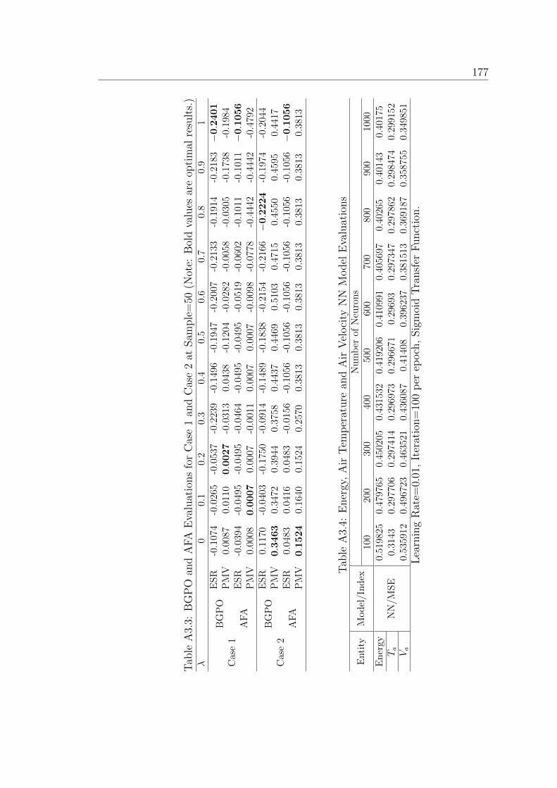
177
Tab
leA
3.3:
BG
PO
and
AFA
Eva
luat
ions
for
Cas
e1
and
Cas
e2
atSam
ple
=50
(Not
e:B
old
valu
esar
eop
tim
alre
sult
s.)
λ0
0.1
0.2
0.3
0.4
0.5
0.6
0.7
0.8
0.9
1
Cas
e1
BG
PO
ESR
-0.1
074
-0.0
265
-0.0
537
-0.2
239
-0.1
496
-0.1
947
-0.2
007
-0.2
133
-0.1
914
-0.2
183−
0.2
401
PM
V0.
0087
0.01
100.0
027
-0.0
313
0.04
38-0
.120
4-0
.028
2-0
.005
8-0
.030
5-0
.173
8-0
.198
4
AFA
ESR
-0.0
394
-0.0
495
-0.0
495
-0.0
464
-0.0
495
-0.0
495
-0.0
519
-0.0
602
-0.1
011
-0.1
011−
0.1
056
PM
V0.
0008
0.0
007
0.00
07-0
.001
10.
0007
0.00
07-0
.009
8-0
.077
8-0
.444
2-0
.444
2-0
.479
2
Cas
e2
BG
PO
ESR
0.11
70-0
.040
3-0
.175
0-0
.091
4-0
.148
9-0
.183
8-0
.215
4-0
.216
6−
0.2
224
-0.1
974
-0.2
044
PM
V0.3
463
0.34
720.
3944
0.37
580.
4437
0.44
690.
5103
0.47
150.
4550
0.45
950.
4417
AFA
ESR
0.04
830.
0416
0.04
83-0
.015
6-0
.105
6-0
.105
6-0
.105
6-0
.105
6-0
.105
6-0
.105
6−
0.1
056
PM
V0.1
524
0.16
400.
1524
0.25
700.
3813
0.38
130.
3813
0.38
130.
3813
0.38
130.
3813
Tab
leA
3.4:
Ener
gy,
Air
Tem
per
ature
and
Air
Vel
oci
tyN
NM
odel
Eva
luat
ions
Enti
tyM
od
el/I
nd
exN
um
ber
ofN
euro
ns
100
200
300
400
500
600
700
800
900
1000
En
ergy
NN
/MS
E0.
5198
250.
4797
650.
4502
050.
4315
320.
4192
060.
4109
910.
4056
970.
4026
50.
4014
30.
4017
5Ta
0.31
430.
2977
060.
2974
140.
2969
730.
2966
710.
2969
30.
2973
470.
2978
620.
2984
740.
2991
52Va
0.53
5912
0.49
6723
0.46
3521
0.43
6087
0.41
408
0.39
6237
0.38
1513
0.36
9187
0.35
8755
0.34
9851
Lea
rnin
gR
ate=
0.01
,It
erat
ion=
100
per
epoch
,Sig
moi
dT
ransf
erF
unct
ion.


Author’s Publications
Journal Papers
1. D. Zhai, Y. C. Soh and X. Ou, “A Data-Driven Approach for Modeling Predic-
tive Thermal State of Occupants,” IEEE Transactions on Industrial Electronics
(2019). [To be submitted]
2. D. Zhai and Y. C. Soh, “Data Driven Model-based Predictive Control and
Bayesian Optimization for Energy Efficient ACMV Systems,” Applied Energy
(2019). [To be submitted]
3. D. Zhai, T. Chaudhuri and Y. C. Soh, “Modeling and optimization of different
sparse augmented firefly algorithms for acmv systems under two case studies,”
Building and Environment, vol. 125, pp. 129-142, 2017.
4. D. Zhai and Y. C. Soh, “Balancing indoor thermal comfort and energy con-
sumption of acmv systems via sparse swarm algorithms in optimizations,” En-
ergy and Buildings, vol. 149, pp. 1-15, 2017.
5. T. Chaudhuri, D. Zhai, Y. C. Soh, H. Li and L. Xie “Random forest based
thermal comfort prediction from gender-specific physiological parameters using
180
wearable sensing technology,” Energy and Buildings, vol. 166, pp. 391-406,
2018.
6. T. Chaudhuri, D. Zhai, Y. C. Soh, H. Li and L. Xie “Thermal comfort pre-
diction using normalized skin temperature in a uniform built environment,”
Energy and Buildings, vol. 159, pp. 426-440, 2017.
7. X. Ou, W. Cai, X. He and D. Zhai, “Experimental investigations on heat and
mass transfer performances of a liquid desiccant cooling and dehumidification
system,” Applied Energy, vol. 220, pp. 164-175, 2018.
8. X. Ou, W. Cai, X. He, X. Wang and D. Zhai, “A dynamic modeling of liquid
desiccant cooling and dehumidification system for control and optimization,”
Energy and Buildings, vol. 163, pp. 44-57, 2017.
9. C. Jiang, Y. C. Soh, H. Li, M. K. Masood, Z. Wei, X. Zhou and D. Zhai, “CFD
results calibration from sparse sensor observations with a case study for indoor
thermal map,” Building and Environment, vol. 117, pp. 166-177, 2017.

181
Conference Papers
1. D. Zhai, T. Chaudhuri, Y. C. Soh, X. Ou and C. Jiang, “Improvement of
Energy Efficiency of Markov ACMV Systems based on PTS Information of
Occupants,” IEEE World Congress on Computational Intelligence (WCCI), Rio
de Janeiro, Brazil, 2018.
2. D. Zhai, T. Chaudhuri and Y. C. Soh, “Energy efficiency improvement with
k-means approach to thermal comfort for acmv systems of smart buildings,”
IEEE Asian Conference on Energy, Power and Transportation Electrification
(ACEPT), pp. 203-208, Singapore, 2017.
3. D. Zhai and Y. C. Soh, “Balancing indoor thermal comfort and energy con-
sumption of air-conditioning and mechanical ventilation systems via sparse Fire-
fly algorithm optimization,” IEEE 30th International Joint Conference on Neu-
ral Networks (IJCNN), pp. 1488-1494, Anchorage, Alaska, U.S.A., 2017.
4. D. Zhai, Y. C. Soh and W. Cai, “Operating points as communication bridge
between energy evaluation with air temperature and velocity based on extreme
learning machine (ELM) models,” IEEE 11th International Conference on In-
dustrial Electronics and Applications (ICIEA), pp. 712-716, Hefei, Anhui, Chi-
na, 2016.
5. D. Zhai and Y. C. Soh, “Research on indoor air-flow measurements and predic-
tions with different methods,” International OSA Network of Students (IONS),
The Optical Society, pp. 52-56, Nanjing, Jiangsu, China, 2015.
6. T. Chaudhuri, D. Zhai, Y. C. Soh, H. Li, L. Xie and X. Ou, “Convolutional
Neural Network and Kernel Methods for Occupant Thermal State Detection

182
using Wearable Technology,” IEEE World Congress on Computational Intelli-
gence (WCCI), Rio de Janeiro, 2018.

Bibliography
[1] The paris protocol - a blueprint for tackling global climate change beyond 2020.
European Commission, 2015.
[2] Herve Abdi and Lynne J. Williams. Principal component analysis. Computa-
tional Statistics, Wiley, 2, 2010.
[3] Adriana Acosta, Ana I. Gonzalez, Jesus M. Zamarreno, and Victor Alvarez.
Energy savings and guaranteed thermal comfort in hotel rooms through nonlinear
model predictive controllers. Energy and Buildings, ELSEVIER, 129:59–68, 2016.
doi: 10.1016/j.enbuild.2016.07.061.
[4] Ahmed Qasim Ahmed, Shian Gao, and Ali Khaleel Kareem. Energy saving and
indoor thermal comfort evaluation using a novel local exhaust ventilation system
for office rooms. Applied Thermal Engineering, ELSEVIER, 110:821–834, 2017.
[5] A. Arabali, M. Ghofrani, M. Etezadi-Amoli, M. S. Fadali, and Y. Baghzouz.
Genetic-algorithm-based optimization approach for energy management. IEEE
Transactions on Power Delivery, 28:162–170, 2012. doi: 10.1109/TPWRD.2012.
2219598.
[6] ASHRAE. Standard 55-2013 : Thermal environmental conditions for human
occupancy. 2013.
184 BIBLIOGRAPHY
[7] Ruben Baetens, Roel De Coninck, Juan Van Roy, Bart Verbruggen, Johan
Driesen, Lieve Helsen, and Dirk Saelens. Assessing electrical bottlenecks at feed-
er level for residential net zero-energy buildings by integrated system simulation.
Applied Energy, ELSEVIER, 96:74–83, 2012.
[8] Saadia Barbhuiya and Salim Barbhuiya. Thermal comfort and energy consump-
tion in a uk educational building. Building and Environment, ELSEVIER, 68:
1–11, 2013.
[9] Christopher M. Bishop. Neural networks for pattern recognition. Oxford univer-
sity press, 1995.
[10] Christopher M. Bishop. Pattern Recognition and Machine Learning. Springer,
2006.
[11] Stephen P. Boyd and Lieven Vandenberghe. Convex Optimization. Cambridge
University Press, 2004.
[12] Eric Brochu, Vlad M. Cora, and Nando de Freitas. A tutorial on bayesian
optimization of expensive cost functions, with application to active user modeling
and hierarchical reinforcement learning. arXiv.org, 2010. doi: arxiv.org/abs/
1012.2599.
[13] Edited by Geoffrey Hinton and Terrence J. Sejnowski. Unsupervised Learning:
Foundations of Neural Computation. The MIT Press, 1999.
[14] C.G. Cassandras and S. Lafortune. Introduction to Discrete Event Systems.
SpringerLink Engineering (2009). ISBN 9780387333328.
[15] Kristen S. Cetin, Lance Manuel, and Atila Novoselac. Effect of technology-
enabled time-of-use energy pricing on thermal comfort and energy use in
BIBLIOGRAPHY 185
mechanically-conditioned residential buildings in cooling dominated climates.
Building and Environment, ELSEVIER, 96:118–130, 2016. doi: 10.1016/j.
buildenv.2015.11.012.
[16] N Charkoudian. Skin blood flow in adult human thermoregulation: how it works,
when it does not, and why. In Mayo Clinic Proceedings, pages 603–612, 2003.
doi: 10.4065/78.5.603.
[17] Tanaya Chaudhuri, Deqing Zhai, Yeng Chai Soh, Hua Li, and Lihua Xie. Ther-
mal comfort prediction using normalized skin temperature in a uniform built
environment. Energy and Buildings, ELSEVIER, 159:426 – 440, 2018. doi:
10.1016/j.enbuild.2017.10.098.
[18] Xiao Chen, Qian Wang, and Jelena Srebric. Occupant feedback based mod-
el predictive control for thermal comfort and energy optimization: A chamber
experimental evaluation. Applied Energy, ELSEVIER, 164:341–351, 2016. doi:
10.1016/j.apenergy.2015.11.065.
[19] Joon-Ho Choi and Vivian Loftness. Investigation of human body skin tempera-
tures as a bio-signal to indicate overall thermal sensations. Building and Envi-
ronment, ELSEVIER, 58:258–269, 2012. doi: 10.1016/j.buildenv.2012.07.003.
[20] Joon-Ho Choi and Vivian Loftness. Investigation of human body skin tem-
peratures as a bio-signal to indicate overall thermal sensations. Building and
Environment, ELSEVIER, 58:258–269, 2012.
[21] Changzhi Dai, Hui Zhang, Edward Arens, and Zhiwei Lian. Machine learning
approaches to predict thermal demands using skin temperatures: Steady-state
conditions. Building and Environment, ELSEVIER, 114:1–10, 2017. doi: 10.
1016/j.buildenv.2016.12.005.

186 BIBLIOGRAPHY
[22] Lyrian Daniel, Terence Williamson, and Veronica Soebarto. Comfort-based
performance assessment methodology for low energy residential buildings in
australia. Building and Environment, ELSEVIER, 111:169–179, 2017. doi:
10.1016/j.buildenv.2016.10.023.
[23] Wenyong Dong and MengChu Zhou. Gaussian classifier-based evolutionary s-
trategy for multimodal optimization. IEEE Transactions on Neural Networks
and Learning Systems, 25:1200–1216, 2014.
[24] Jean-Michel Dussault, Maarten Sourbron, and Louis Gosselin. Reduced energy
consumption and enhanced comfort with smartwindows: Comparison between
quasi-optimal, predictive andrule-based control strategies. Energy and Buildings,
ELSEVIER, 127:680–691, 2016. doi: 10.1016/j.enbuild.2016.06.024.
[25] Andries P. Engelbrecht. Computational Intelligence: An Introduction. Wiley
Publishing 2007, 2007.
[26] P.O. Fanger. Thermal comfort: Analysis and applications in environmental en-
gineering. Danish Technical Press, 1970.
[27] Mohammad Hassan Fathollahzadeh, Ghassem Heidarinejad, and Hadi Pasdar-
shahri. Prediction of thermal comfort, iaq, and energy consumption in a dense
occupancy environment with the under floor air distribution system. Building and
Environment, ELSEVIER, 90:96–104, 2015. doi: 10.1016/j.buildenv.2015.03.019.
[28] Clifford Conrad Federspiel. User-adaptable and minimum-power thermal comfort
control. Massachusetts Institute of Technology, 1992.
[29] P.M. Ferreira, A.E. Ruano, S. Silva, and E.Z.E. Conceicao. Neural networks

BIBLIOGRAPHY 187
based predictive control for thermal comfort and energy savings in public build-
ings. Energy and Buildings, ELSEVIER, 55:238–251, 2012.
[30] Antonio Figueiredo, Jose Figueira, Romeu Vicente, and Rui Maio. Thermal
comfort and energy performance: Sensitivity analysis to apply the passive house
concept to the portuguese climate. Building and Environment, ELSEVIER, 103:
276–288, 2016.
[31] Katarzyna Gadyszewska-Fiedoruk. Correlations of air humidity and carbon diox-
ide concentration in the kindergarten. Energy and Buildings, ELSEVIER, 62:
45–50, 2013.
[32] Ali Ghahramani, Guillermo Castro, Burcin Becerik-Gerber, and Xinran Yu. In-
frared thermography of human face for monitoring thermoregulation performance
and estimating personal thermal comfort. Building and Environment, ELSEVI-
ER, 109:1–11, 2016. doi: 10.1016/j.buildenv.2016.09.005.
[33] Ian Goodfellow, Yoshua Bengio, and Aaron Courville. Deep Learning. The MIT
Press, 2016. http://www.deeplearningbook.org.
[34] David J. Hand. Principles of data mining. Drug safety, 30(7):621–622, 2007.
[35] Yingdong He, Nianping Li, Linxuan Zhou, Kuan Wang, and Wenjie Zhang. Ther-
mal comfort and energy consumption in cold environment with retrofitted huo-
tong (warm-barrel). Building and Environment, ELSEVIER, 112:285–295, 2017.
doi: 10.1016/j.buildenv.2016.11.044.
[36] Yueer He, Meng Liu, Thomas Kvan, and Shini Peng. An enthalpy-based energy
savings estimation method targeting thermal comfort level in naturally ventilated

188 BIBLIOGRAPHY
buildings in hot-humid summer zones. Applied Energy, ELSEVIER, 187:717–731,
2017. doi: 10.1016/j.apenergy.2016.11.098.
[37] J. C. Ho, G. Jindal, and M. Low. Singapore’s intended nationally determined
contribution for cop21 climate conference in paris. Energy Studies Institute,
2015.
[38] John Henry Holland. Adaptation in Natural and Artificial Systems. University
of Michigan Press, 1975.
[39] David W. Hosmer and Stanley Lemeshow. Applied Logistic Regression. A Wiley-
Interscience Publication, 2000.
[40] Tapas Kanungo, David M. Mount, Nathan S. Netanyahu, Christine D. Piatko,
Ruth Silverman, and Angela Y. Wu. An efficient k-means clustering algorith-
m: Analysis and implementation. IEEE Transactions on Pattern Analysis and
Machine Intelligence, 24(7):881–892, 2002.
[41] James Kennedy and Russell Eberhart. Particle swarm optimization. In IEEE
international conference on neural networks, pages 1942–1948, 1995. doi: 10.
1109/ICNN.1995.488968.
[42] Jeong Tai Kim, Ji Hyun Lim, Sun Ho Cho, and Geun Young Yun. Development
of the adaptive pmv model for improving prediction performances. Energy and
Buildings, ELSEVIER, 98:100–105, 2015.
[43] Jimin Kim, Taehoon Hong, Jaemin Jeong, Choongwan Koo, and Kwangbok
Jeong. An optimization model for selecting the optimal green systems by consid-
ering the thermal comfort and energy consumption. Applied Energy, ELSEVIER,
169:682–695, 2016. doi: 10.1016/j.apenergy.2016.02.032.

BIBLIOGRAPHY 189
[44] N. Klepeis. The national human activity pattern survey (nhaps) - a resource
for assessing exposure to environmental pollutants. National Exposure Research
Laboratory, U.S. Environmental Protection Agency.
[45] Andrew Kusiak. Intelligent manufacturing systems. PRENTICE HALL PRESS,
200 OLD TAPPAN ROAD, OLD TAPPAN, NJ 07675, USA, 1990, 448, 1990.
[46] Andrew Kusiak and Mingyang Li. Cooling output optimization of an air handling
unit. Applied Energy, ELSEVIER, pages 901–909, 2010. doi: 10.1016/j.apenergy.
2009.06.010.
[47] Ranald Lawrence and Charlotte Keime. Bridging the gap between energy
and comfort: Post-occupancy evaluation of two higher-education buildings in
sheffield. Energy and Buildings, ELSEVIER, 130:651–666, 2016.
[48] A. Leavey, Y. Fu, M. Sha, A. Kutta, C. Lu, W. Wang, B. Drake, Y. Chen,
and P. Biswas. Air quality metrics and wireless technology to maximize the
energy efficiency of hvac in a working auditorium. Building and Environment,
ELSEVIER, pages 287–297, 2015.
[49] Jiajia Li, Botao Wang, and Guoren Wang. Elm based efficient probabilistic
threshold query on uncertain data. In Proceedings of ELM-2014 Volume 1-
Algorithms and Theories, pages 71–80, 2014. doi: 10.1007/978-3-319-14063-6 7.
[50] Kangji Li, Chenglei Hu, Guohai Liu, and Wenping Xue. Building’s electricity
consumption prediction using optimized artificial neural networks and principal
component analysis. Energy and Buildings, ELSEVIER, 108:106–113, 2015. doi:
10.1016/j.enbuild.2015.09.002.
190 BIBLIOGRAPHY
[51] Shin-Yeu Lin, Shih-Ching Chiu, and Wei-Yuan Chen. Simple automatic supervi-
sory control system for office building based on energy-saving decoupling indoor
comfort control. Energy and Buildings, ELSEVIER, 86:7–15, 2015.
[52] Weiwei Liu, Zhiwei Lian, and Qihong Deng. Use of mean skin temperature in
evaluation of individual thermal comfort for a person in a sleeping posture under
steady thermal environment. Indoor and Built Environment, ELSEVIER, 24:
489–499, 2014. doi: 10.1177/1420326X14527975.
[53] Weiwei Liu, Zhiwei Lian, and Qihong Deng. Use of mean skin temperature in
evaluation of individual thermal comfort for a person in a sleeping posture under
steady thermal environment. Indoor and Built Environment, 24(4):489499, 2015.
doi: 10.1177/1420326X14527975.
[54] Ning Mao, Mengjie Song, and Shiming Deng. Application of topsis method in
evaluating the effects of supply vane angle of a task/ambient air conditioning
system on energy utilization and thermal comfort. Applied Energy, ELSEVIER,
180:536–545, 2016.
[55] Jin Woo Moon and Sung Kwon jung. Development of a thermal control algo-
rithm using artificial neural network models for improved thermal comfort and
energy efficiency in accommodation buildings. Applied Thermal Engineering,
ELSEVIER, 103:1135–1144, 2016.
[56] NEA and Singapore. Stricter energy performance standard-
s for air-conditioners from september 2016. http://www.
nea.gov.sg/corporate-functions/newsroom/news-releases/
stricter-energy-performance-standards-for-air-conditioners-from-september-2016,
Accessed: 2016-12-20.

BIBLIOGRAPHY 191
[57] Andrew Ng and Dan Boneh. Cs229: Machine learning, 2017. URL http://
cs229.stanford.edu/.
[58] Adam ODonovan, P.D. OSullivan, and Michael D. Murphy. A field study of
thermal comfort performance for a slotted louvreventilation system in a low
energy retrofit. Energy and Buildings, ELSEVIER, 135:312–323, 2017.
[59] Omkar M Parkhi, Andrea Vedaldi, C. V. Jawahar, and Andrew Zisserman. The
truth about cats and dogs. In Proceedings of IEEE International Conference on
Computer Vision, pages 1427–1434, 2011.
[60] Marco Pritoni, Kiernan Salmon, Angela Sanguinetti, Joshua Morejohn, and
Mark Modera. Occupant thermal feedback for improved efficiency in univer-
sity buildings. Energy and Buildings, ELSEVIER, 144:241–250, 2017. doi:
10.1016/j.enbuild.2017.03.048.
[61] C. E. Rasmussen and C. K. I. Williams. Gaussian Processes for Machine Learn-
ing. MIT Press, Cambridge, Massachusetts,, 2006.
[62] John O. Rawlings, Sastry G. Pantula, and David A. Dickey. Applied Regression
Analysis. Springer, 1988.
[63] Frank Rosenblatt. The perceptron - a perceiving and recognizing automaton.
Report, Cornell Aeronautical Laboratory, pages 85–460–1, 1957.
[64] Antonio E. Ruano, Shabnam Pesteh, Sergio Silva, Helder Duate, Goncalo Mestre,
Pedro M. Ferreira, Hamid R. Khosravani, and Ricardo Horta. The imbpc hvac
system: A complete mbpc solution for existing hvac systems. Energy and Build-
ings, ELSEVIER, 120:145–158, 2016.

192 BIBLIOGRAPHY
[65] Dirk Saelens, Jan Carmeliet, and Hugo Hens. Energy performance assessment
of multiple-skin facades. HVACR Research, 9:167–185, 2003.
[66] Dirk Saelens, Wout Parys, and Ruben Baetens. Energy and comfort performance
of thermally activated building systems including occupant behavior. Building
and Environment, 46:835–848, 2011.
[67] Sally Shahzad, John Brennan, Dimitris Theodossopoulos, Ben Hughes, and
John Kaiser Calautit. Energy and comfort in contemporary open plan and tra-
ditional personal offices. Applied Energy, ELSEVIER, 185:1542–1555, 2017.
[68] Max H. Sherman. Simplified model of thermal comfort. Energy and Buildings,
ELSEVIER, 8, 1985.
[69] Jonathon Shlens. A tutorial on principal component analysis. arXiv, 2014.
[70] David Silver, Julian Schrittwieser, Karen Simonyan, Ioannis Antonoglou, A-
ja Huang, Arthur Guez, Thomas Hubert, Lucas Baker, Matthew Lai, Adrian
Bolton, Yutian Chen, Timothy Lillicrap, Fan Hui, Laurent Sifre, George van den
Driessche, Thore Graepel, and Demis Hassabis. Mastering the game of go with-
out human knowledge. Nature, 550:354–359, 2017. doi: 10.1038/nature24270.
[71] Soo Young Sim, Myung Jun Koh, Kwang Min Joo, Seungwoo Noh, Sangyun
Park, Youn Ho Kim, and Kwang Suk Park. Estimation of thermal sensation
based on wrist skin temperatures. Sensors (Basel), 16, 2016. doi: 10.3390/
s16040420.
[72] Adrian Streinu-Cercel, Sergiu Costoiu, Maria Mrza, Anca Streinu-Cercel, and
Monica Mrza. Models for the indices of thermal comfort. Journal of Medicine
and Life, X, 2017.

BIBLIOGRAPHY 193
[73] Richard S. Sutton and Andrew G. Barto. Reinforcement Learning: An Introduc-
tion. The MIT Press, 1998.
[74] Satoru Takada, Sho Matsumoto, and Takayuki Matsushita. Prediction of whole-
body thermal sensation in the non-steady state based on skin temperature. Build-
ing and Environment, ELSEVIER, 68:123–133, 2013. doi: 10.1016/j.buildenv.
2013.06.004.
[75] Toolbox. Clothing and thermal insulation. http://www.engineeringtoolbox.
com/clo-clothing-thermal-insulation-d_732.html, Accessed: 2017-06-20.
[76] Toolbox. Metabolic rate. http://www.engineeringtoolbox.com/
met-metabolic-rate-d_733.html, Accessed: 2017-06-20.
[77] Allen M. Turing. Computing machinery and intelligence. Mind, 1950.
[78] Ali Vedavarz, Sunil Kumar, and Muhammed Iqbal Hussain. HVAC: Handbook
of Heating, Ventilation and Air Conditioning for Design and Implementation.
SpringerLink Engineering (2009). ISBN 0831131632,9780831131630.
[79] Yang Wang, Jens Kuckelkorn, Fu-Yun Zhao, Di Liu, Alexander Kirschbaum, and
Jun-Liang Zhang. Evaluation on classroom thermal comfort and energy perfor-
mance of passive school building by optimizing hvac control systems. Building
and Environment, ELSEVIER, 89:86–106, 2015. doi: 10.1016/j.buildenv.2015.
02.023.
[80] D. Randall Wilson and Tony R. Martinez. The general inefficiency of batch
training for gradient descent learning. Neural Networks, ELSEVIER, 16:1429–
1451, 2003.

194 BIBLIOGRAPHY
[81] D.H. Wolpert and W.G. Macready. No free lunch theorems for optimization.
IEEE Transactions on Evolutionary Computation, 1:67–82, 1997.
[82] L. T. Wong, K. W. Mui, and C. T. Cheung. Bayesian thermal comfort mod-
el. Building and Environment, ELSEVIER, 82:171–179, 2014. doi: 10.1016/j.
buildenv.2014.08.018.
[83] Jing Xiong, Xin Zhou, Zhiwei Lian, Jianxiong You, and Yanbing Lin. Thermal
perception and skin temperature in different transient thermal environments in
summer. Energy and Buildings, ELSEVIER, 128:155–163, 2016. doi: 10.1016/j.
enbuild.2016.06.085.
[84] Xin Yan and Xiaogang Su. Linear regression analysis: theory and computing.
World Scientific, 2009.
[85] Xin-She Yang. Nature-inspired metaheuristic algorithms. 1st ed. Frome, UK:
Luniver Press, 2008.
[86] Xin-She Yang. Firefly algorithms for multimodal optimisation. In Proceedings
fifth symposium on stochastic algorithms, foundations and applications, pages
169–178, 2009.
[87] Xin-She Yang. Nature-Inspired Optimization Algorithms. ELSEVIER, 2014.
[88] Wei Yu, Baizhan Li, Hongyuan Jia, Ming Zhang, and Di Wang. Application
of multi-objective genetic algorithm to optimize energy efficiency and thermal
comfort in building design. Energy and Buildings, ELSEVIER, 88:135–143, 2015.
doi: 10.1016/j.enbuild.2014.11.063.
[89] Wim Zeiler, Michal Vesely, Derek Vissers, and Rongling Li. Thermal response
of different body parts: The fingertip as control sensor for personalized heating.

BIBLIOGRAPHY 195
Energy Procedia, ELSEVIER, 78:2766–2771, 2015. doi: 10.1016/j.egypro.2015.
11.622.
[90] Deqing Zhai and Yeng Chai Soh. Balancing indoor thermal comfort and energy
consumption of acmv systems via sparse swarm algorithms in optimizations.
Energy and Buildings, ELSEVIER, 149:1–15, 2017. doi: 10.1016/j.enbuild.2017.
05.019.
[91] Deqing Zhai and Yeng Chai Soh. Balancing indoor thermal comfort and energy
consumption of air-conditioning and mechanical ventilation systems via sparse
firefly algorithm optimization. In Proceedings of IEEE Joint Conference on Neu-
ral Networks, pages 1488–1494, 2017. doi: 10.1109/IJCNN.2017.7966028.
[92] Deqing Zhai, Yeng Chai Soh, and Wenjian Cai. Operating points as commu-
nication bridge between energy evaluation with air temperature and velocity
based on extreme learning machine (elm) models. In Proceedings of IEEE Con-
ference on Industrial Electronics and Applications, pages 712–716, 2016. doi:
10.1109/ICIEA.2016.7603675.
[93] Deqing Zhai, Tanaya Chaudhuri, and Yeng Chai Soh. Energy Efficiency Improve-
ment with k-means Approach to Thermal Comfort for ACMV Systems of Smart
Buildings. In IEEE Asian Conference on Energy, Power and Transportation
Electrification (ACEPT), pages 203–208, October 2017.
[94] Deqing Zhai, Tanaya Chaudhuri, and Yeng Chai Soh. Modeling and optimization
of different sparse augmented firefly algorithms for acmv systems under two case
studies. Building and Environment, ELSEVIER, 125:129–142, 2017. doi: 10.
1016/j.buildenv.2017.08.032.

196 BIBLIOGRAPHY
[95] Deqing Zhai, Tanaya Chaudhuri, Yeng Chai Soh, Xianhua Ou, and Chaoyang
Jiang. Improvement of energy efficiency of markov acmv systems based on pts in-
formation of occupants. In IEEE World Congress on Computational Intelligence
(WCCI), pages 3303–3309, July 2018.
[96] Hui Zhang, Edward Arens, Charlie Huizenga, and Taeyoung Han. Thermal
sensation and comfort models for non-uniform and transient environments, part
iii: Whole-body sensation and comfort. Building and Environment, ELSEVIER,
45:299 – 410, 2010. doi: 10.1016/j.buildenv.2009.06.020.
[97] Weiwei Zhang, Jian Sun, and Xiaoou Tang. Cat head detection - how to effec-
tively exploit shape and texture features. In Proceedings of European Conference
on Computer Vision, pages 802–816, 2008.
[98] Yuanhui Zhang. Indoor Air Quality Engineering. CRC Press, 2004.
[99] MengChu Zhou and Kurapati Venkatesh. Modeling, Simulation, And Control
Of Flexible Manufacturing Systems: A Petri Net Approach. World Scientific
Publishing Co Pte Ltd, 1999.