mixed procedurally generated creatures

Mixed Procedurally Generated Creatures

Andre Goncalo Caetano Soares

Thesis to obtain the Master of Science Degree in

Information Systems and Computer Engineering

Supervisor: Prof. Carlos Antonio Roque Martinho

Examination Committee

Chairperson: Prof. Antonio Manuel Ferreira Rito da SilvaSupervisor: Prof. Carlos Antonio Roque Martinho

Member of the Committee: Prof. Ana Paula Boler Claudio

November 2019

Acknowledgments

I would like to first and foremost thank my parents, Nelson and Odete, for all the patience and love

they have given me through all of my life and without whom this work would not be possible and also

to my little brother, Diogo, that has provided company while I worked and to my aunt, Andreia, who has

given me confidence on my work and knowledge. To my girlfriend, Catia, for being patient and listening

to me even though sometimes I am pretty sure she did not understand a word of what I was talking

about, for being supportive and protective of me and this work and for being there when I needed the

most. To my cat, Tobias, who has let me scratch him, pet him and has bitten and scratched me countless

times, a big thank you from the bottom of my heart for keeping me company and distracted.

To Professor Carlos Martinho, I have to thank for everything I’ve experienced in this MSc, mainly in

the Games specialization, but also due to the patience and work that he has done with me for this thesis

and all the guidance provided, helping me getting past blocks that I’ve found along the way. I hope that

you keep enjoying games as much as we all do and that you know that you have helped me a lot.

To my grandparents I would like to say thank you for taking care of me and for the help you have

provided.

To my friends, I would like to thank you for all the laughs and confused looks when I talked about this

work with you. But mostly I would like to thank you for all the hours of entertainment that helped keep

me sane even though you all have your own thesis and classes to attend to.

To everyone involved with this work and/or reading this work, a big thank you for taking your time to

read my work and I hope that this can be of help to future game developers.

Abstract

Animations are a core component of video games. Animations typically require dedicated animators

and are relatively inflexible, making it extremely difficult to animate a character without enforcing strict

restrictions on the virtual world where it is placed. We propose a framework to explore the procedural

generation of animations in arbitrary tridimensional virtual worlds, by using neuroevolution to create and

evolve neural networks that output forces at a creature’s skeleton joints in order to produce motion and

movement that are credible and physically coherent with the virtual world topology and the creature’s

state. Evaluation was done by selecting tasks for which our framework was able to generate animations

that are different between each other but that achieve the same result proving that neuroevolution can

offer different solutions to animation problems even when using different body topologies which were

also able to achieve the same task using the same fitness method.

Keywords

Animation; Procedural Animation; Procedural Content Generation; Artificial Intelligence; Neuroevolution;

Neural Networks; NEAT;

iii

Resumo

As animacoes sao uma das componentes essenciais num video jogo 3D e tipicamente requerem ani-

madores dedicados e sao relativamente inflexiveis, forcando o uso de restricoes a nivel do mundo virtual

onde sao usadas. Nesta tese, propomos e demonstramos uma framework que permite a exploracao de

animacoes, geradas de forma automatica tendo em conta um objectivo, em mundos virtuais arbitrarios,

usando neuroevolucao para criar e evoluir redes neurais as quais calculam valores para serem usados

como forcas nas juntas do esqueleto de uma criatura, produzindo movimento que sao fisicamente co-

erentes com a tipologia do mundo e o estado atual da criatura. A avaliacao e feita atraves da seleccao

de diferentes tarefas para as quais a nossa framework foi capaz de gerar animacoes que sao difer-

entes entre si mas que alcancam o mesmo resultado, provando que a neuroevolucao pode oferecer

solucoes diferentes para problemas de animacao mesmo quando se usam tipos de corpos diferentes

que conseguiram resolver a mesma tarefa usando os metodos de avaliacao usados previamente.

Palavras Chave

Animacao; Animacao Procedural; Geracao de Conteudo Procedural; Inteligencia Artificial; Neuroevolucao;

Redes Neurais; NEAT;

v

Contents

1 Introduction 1

1.1 Motivation . . . . . . . . . . . . . . . . . . . . . . . . . . . . . . . . . . . . . . . . . . . . . 3

1.2 The Problem . . . . . . . . . . . . . . . . . . . . . . . . . . . . . . . . . . . . . . . . . . . 4

1.3 Hypothesis . . . . . . . . . . . . . . . . . . . . . . . . . . . . . . . . . . . . . . . . . . . . 4

1.4 Contributions . . . . . . . . . . . . . . . . . . . . . . . . . . . . . . . . . . . . . . . . . . . 5

1.5 Document outline . . . . . . . . . . . . . . . . . . . . . . . . . . . . . . . . . . . . . . . . . 5

2 Background 7

2.1 Animation Background . . . . . . . . . . . . . . . . . . . . . . . . . . . . . . . . . . . . . . 9

2.2 Machine Learning for Animation . . . . . . . . . . . . . . . . . . . . . . . . . . . . . . . . 11

2.2.1 Neural Network Models . . . . . . . . . . . . . . . . . . . . . . . . . . . . . . . . . 12

2.2.2 Genetic Algorithms . . . . . . . . . . . . . . . . . . . . . . . . . . . . . . . . . . . . 13

2.2.3 Concluding Remark . . . . . . . . . . . . . . . . . . . . . . . . . . . . . . . . . . . 13

3 Related Work 15

3.1 Phase-Functioned Neural Networks for Character Control . . . . . . . . . . . . . . . . . . 17

3.2 Mode-Adaptive Neural Networks for Quadruped Motion Control . . . . . . . . . . . . . . . 17

3.3 Evolving Virtual Creatures . . . . . . . . . . . . . . . . . . . . . . . . . . . . . . . . . . . . 18

3.4 NeuroEvolution of Augmenting Topologies . . . . . . . . . . . . . . . . . . . . . . . . . . . 19

3.5 Discussion . . . . . . . . . . . . . . . . . . . . . . . . . . . . . . . . . . . . . . . . . . . . 24

4 Computational Model 27

4.1 Development Environment . . . . . . . . . . . . . . . . . . . . . . . . . . . . . . . . . . . . 29

4.1.1 C++17 . . . . . . . . . . . . . . . . . . . . . . . . . . . . . . . . . . . . . . . . . . . 29

4.1.2 Unreal Engine 4 (UE4) . . . . . . . . . . . . . . . . . . . . . . . . . . . . . . . . . . 30

4.1.3 PhysX . . . . . . . . . . . . . . . . . . . . . . . . . . . . . . . . . . . . . . . . . . . 30

4.2 NEATAnim . . . . . . . . . . . . . . . . . . . . . . . . . . . . . . . . . . . . . . . . . . . . . 30

4.2.1 Architecture . . . . . . . . . . . . . . . . . . . . . . . . . . . . . . . . . . . . . . . . 33

4.3 MPGCreatures PhysX Simulator . . . . . . . . . . . . . . . . . . . . . . . . . . . . . . . . 36

4.3.1 Architecture . . . . . . . . . . . . . . . . . . . . . . . . . . . . . . . . . . . . . . . . 38

vii

4.3.2 Simulation & Simulation Manager . . . . . . . . . . . . . . . . . . . . . . . . . . . . 41

4.4 MPGCreatures in UE4 . . . . . . . . . . . . . . . . . . . . . . . . . . . . . . . . . . . . . . 42

4.4.1 Architecture . . . . . . . . . . . . . . . . . . . . . . . . . . . . . . . . . . . . . . . . 43

4.4.2 Setting up creatures and levels . . . . . . . . . . . . . . . . . . . . . . . . . . . . . 47

4.4.3 Concluding Remarks . . . . . . . . . . . . . . . . . . . . . . . . . . . . . . . . . . . 49

5 Evaluation 51

5.1 Evaluation methodology . . . . . . . . . . . . . . . . . . . . . . . . . . . . . . . . . . . . . 53

5.2 Tests . . . . . . . . . . . . . . . . . . . . . . . . . . . . . . . . . . . . . . . . . . . . . . . . 53

5.2.1 Cubes . . . . . . . . . . . . . . . . . . . . . . . . . . . . . . . . . . . . . . . . . . . 53

5.2.2 Walking spiders . . . . . . . . . . . . . . . . . . . . . . . . . . . . . . . . . . . . . 56

5.2.3 Human character raising an arm . . . . . . . . . . . . . . . . . . . . . . . . . . . . 58

5.2.4 Standing up Quad Bot . . . . . . . . . . . . . . . . . . . . . . . . . . . . . . . . . . 62

5.2.5 Standing Spider Bot . . . . . . . . . . . . . . . . . . . . . . . . . . . . . . . . . . . 63

5.2.6 Discussion . . . . . . . . . . . . . . . . . . . . . . . . . . . . . . . . . . . . . . . . 64

6 Conclusion 65

6.1 System Limitations and Future Work . . . . . . . . . . . . . . . . . . . . . . . . . . . . . . 68

A Appendix A 73

viii

List of Figures

3.1 Representation of a genome in NEAT. The first list shows the genes and the type of

genes along with an identification number to use in a connection. The second list shows

the connections between genes, the weight of a connection, the innovation number and

the status of the connection. . . . . . . . . . . . . . . . . . . . . . . . . . . . . . . . . . . . 20

3.2 The Competing Conventions Problem - When using TWEANNs, it is possible to arrive at

the same solution with different representation of the topology. When Parent 1 with hidden

nodes [A B C] and parent 2 with hidden nodes [C B A] try to breed and produce offspring,

there is a chance that some of the off-springs omit information that was needed on both

parents to solve the problem. . . . . . . . . . . . . . . . . . . . . . . . . . . . . . . . . . . 21

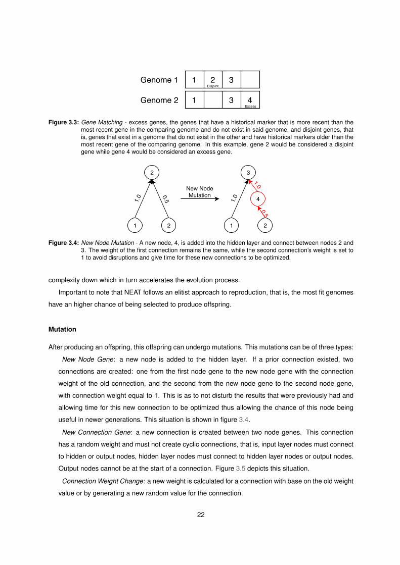
3.3 Gene Matching - excess genes, the genes that have a historical marker that is more recent

than the most recent gene in the comparing genome and do not exist in said genome, and

disjoint genes, that is, genes that exist in a genome that do not exist in the other and have

historical markers older than the most recent gene of the comparing genome. In this

example, gene 2 would be considered a disjoint gene while gene 4 would be considered

an excess gene. . . . . . . . . . . . . . . . . . . . . . . . . . . . . . . . . . . . . . . . . . 22

3.4 New Node Mutation - A new node, 4, is added into the hidden layer and connect between

nodes 2 and 3. The weight of the first connection remains the same, while the second

connection’s weight is set to 1 to avoid disruptions and give time for these new connections

to be optimized. . . . . . . . . . . . . . . . . . . . . . . . . . . . . . . . . . . . . . . . . . 22

3.5 New Connection Mutation - A new connection is added between node 1 and node 4. This

connection starts with a random weight. . . . . . . . . . . . . . . . . . . . . . . . . . . . . 23

3.6 Minimization - The first row genomes are an example of a starting population used in

regular Topology and Weight Evolving Artificial Neural Network (TWEANN)s while the

second row genomes show how NEAT starts out. By starting minimally, NEAT is able to

perform up to seven times faster than by starting with a random population due to the

lower dimensional search space. . . . . . . . . . . . . . . . . . . . . . . . . . . . . . . . . 24

ix

4.1 Delete Link Operator - A random link between two nodes is deleted. This helps keeping

the number of links under control and allowing to explore minimal solutions more effec-

tively as a link that has appeared at the start of the evolution might become unnecessary.

In this case the link between Node 1 and Node 4 has been deleted. . . . . . . . . . . . . 31

4.2 Delete Link Operator with orphaned node - A special case of the delete link operator. If a

node becomes orphaned and is a hidden node, that is, it does not have any incoming link

or outgoing links and it is not a input or output node, it is also deleted from the network. . 32

4.3 Delete Node Operator - Similarly to the delete link operator, a random node is selected

and removed from the network. Any link to or from this node is also removed. This allows

for the reduction of complexity in a network thus speeding up the process of execution. . 32

4.4 The overall architecture and flow of NEATAnim - The first generation is created by the

GenomeManager by cloning a single genome, from which generated genomes form their

organisms by instantiating their phenotype and form a population. This population then

performs the task stipulated by the evaluator. The evaluator measures the performance of

the networks and attributes a fitness value to the organism which is then used to calculate

the next generation of genomes. . . . . . . . . . . . . . . . . . . . . . . . . . . . . . . . . 35

4.5 MPG Creatures PhysX Simulator - The core idea behind the simulator. The simulator

replaces the task and evaluation processes present in NEATAnim with a physically based

simulation. . . . . . . . . . . . . . . . . . . . . . . . . . . . . . . . . . . . . . . . . . . . . 36

4.6 MPG Creatures PhysX Simulator - A snapshot of the simulator running a simulation to

evolve cubes to walk in the positive X direction, noted as blue in the axis seen in the

middle of the world. . . . . . . . . . . . . . . . . . . . . . . . . . . . . . . . . . . . . . . . 37

4.7 MPGCreatures Simulator Overview - Interaction of each of the components. . . . . . . . 38

4.8 Mixed Procedurally Generated Creature (MPGCreature) - Overview of the creature archi-

tecture. . . . . . . . . . . . . . . . . . . . . . . . . . . . . . . . . . . . . . . . . . . . . . . 39

4.9 MPGCreature - Overview of the sensor interface. . . . . . . . . . . . . . . . . . . . . . . . 39

4.10 Sensor to Neural Network Inputs - The sensor outputs are used as inputs to the neural

network. . . . . . . . . . . . . . . . . . . . . . . . . . . . . . . . . . . . . . . . . . . . . . . 40

4.11 Evaluator Interface - The main methods and attributes of the evaluator interface. BestCrea-

ture is a pointer to keep the best creature of the last evaluation. . . . . . . . . . . . . . . . 40

4.12 Creature Farm - Each farm has it’s own separate evolution envoirnment and set of crea-

tures. . . . . . . . . . . . . . . . . . . . . . . . . . . . . . . . . . . . . . . . . . . . . . . . 41

4.13 Simulation - Represents a simulation environment. . . . . . . . . . . . . . . . . . . . . . 42

4.15 SkeletalCreature - the new creature architecture. . . . . . . . . . . . . . . . . . . . . . . 43

x

4.14 MPGCreatures in UE4 - The main conceptual model is very similar to the simulator. Most

of the classes are now run inside UE4 with minimal differences that allow for the function-

ality to be extended to the blueprint system of UE4 for easier use. . . . . . . . . . . . . . 44

4.16 Two different skeletal meshes and their corresponding skeletons shown in white. . . . . . 45

4.17 Example of an initial network- This network possesses a single input node and starts

with the recommended number of hidden nodes, 1. This example network is a simplified

version for just a single joint creature. For a creature with more joints the network input

and hidden layers would stay the same but the output nodes would be N*6 where N is the

number of joints. The network starts with the hidden node connected to all output nodes. 46

4.18 SkeletalNoMeshCreature - Similar to Figure 4.15 but using static meshes as body parts

instead of a mesh and a skeleton. . . . . . . . . . . . . . . . . . . . . . . . . . . . . . . . 46

4.19 Two different topologies of SkeletalNoMeshCreature with their joints visible between static

meshes. . . . . . . . . . . . . . . . . . . . . . . . . . . . . . . . . . . . . . . . . . . . . . . 47

4.20 Creating a new creature - To create a blueprint class to use the framework it should inherit

from the SkeletalCreature class provided. . . . . . . . . . . . . . . . . . . . . . . . . . . . 48

4.21 Adding the skeletal mesh - To create a blueprint class to use the framework it should

inherit from the SkeletalCreature class provided. . . . . . . . . . . . . . . . . . . . . . . . 48

4.22 Creature Farm Settings - This parameters indicate the current number of creatures in

a scene, the number of nodes for each layer of the initial genome, the training time in

seconds and the creature blueprint to be used for the evolution process. . . . . . . . . . . 49

5.1 Initial genome setup - The genome starts with a bias node set to the fixed value of 1.

It contains 6 input sensor nodes that use the value from the eye sensor, the orientation

sensor and the walk sensor. . . . . . . . . . . . . . . . . . . . . . . . . . . . . . . . . . . . 54

5.2 Solution genome - The final genome contains the same nodes but has new connection

links between nodes, including recurrent connections. It has ended with a total of 14 links

from an initial 10. The new links are marked in red. . . . . . . . . . . . . . . . . . . . . . . 55

5.3 The obstacle course test - Creatures start at the center of the scene where the axis

is marked and have the task of reaching the blue circle on the right of the obstacles.

The cube creatures are colored in green when moving and dark green when inactive.

Obstacles are shown in light blue. . . . . . . . . . . . . . . . . . . . . . . . . . . . . . . . 55

5.4 A creature solving the task - At the 28th generation mark a cube was able to dodge the

obstacles and reach the center point. Obstacles are shown in light blue while the cube

that solved the task is colored in red. . . . . . . . . . . . . . . . . . . . . . . . . . . . . . . 56

5.5 Spider Test Scene - The scene is composed of 4 walls, a plane and 84 spider creatures. . 57

5.6 The physics body and angular motor settings used for this test. . . . . . . . . . . . . . . . 57

xi

5.8 The upper arm bone - Every bone below, in the hierarchy, the one marked as orange will

be simulating physics for this test. . . . . . . . . . . . . . . . . . . . . . . . . . . . . . . . 58

5.7 Still images captured on generation 410 of the evolution process. . . . . . . . . . . . . . . 59



5.11 Different behaviors achieved during the same simulation. . . . . . . . . . . . . . . . . . . 63


xii

List of Tables

4.1 Available mutations and their probabilities in NEATAnim. . . . . . . . . . . . . . . . . . . . 33

4.2 Mating types and their probabilities in NEATAnim. . . . . . . . . . . . . . . . . . . . . . . . 34

List of Algorithms

xiii

Listings

A.1 Example of an eye sensor’s get activations() method. . . . . . . . . . . . . . . . . . . 74

xv

Acronyms

PCG Procedural Content Generation

ANN Artificial Neural Networks

NN Neural Networks

NE NeuroEvolution

Mocap Motion Capture

PBA Physically Based Animation

IK Inverse Kinematics

CNN Convolutional Neural Network

TWEANN Topology and Weight Evolving Artificial Neural Network

EANN Evolutionary Artificial Neural Networks

EA Evolutionary Algorithm

ML Machine Learning

GAS Genetic Algorithms

GA Genetic Algorithm

PFNN Phase-Functioned Neural Network

RNN Regressive Neural Networks

NEAT NeuroEvolution of Augmenting Topologies

MANN Mode-Adaptive Neural Network

AccNEAT Accelerated NEAT

xvii

GPGPU General-purpose Computing on Graphics Processing Units

CUDA Compute Unified Device Architecture

CPU Central Processing Unit

NeatENV NEAT Environment

PRNG Pseudo Random Number Generator

MPGCreature Mixed Procedurally Generated Creature

UE4 Unreal Engine 4

xviii

1Introduction

Contents

1.1 Motivation . . . . . . . . . . . . . . . . . . . . . . . . . . . . . . . . . . . . . . . . . . . 3

1.2 The Problem . . . . . . . . . . . . . . . . . . . . . . . . . . . . . . . . . . . . . . . . . . 4

1.3 Hypothesis . . . . . . . . . . . . . . . . . . . . . . . . . . . . . . . . . . . . . . . . . . . 4

1.4 Contributions . . . . . . . . . . . . . . . . . . . . . . . . . . . . . . . . . . . . . . . . . 5

1.5 Document outline . . . . . . . . . . . . . . . . . . . . . . . . . . . . . . . . . . . . . . . 5

1

1.1 Motivation

Animations have always played an important part in video games, with the rise of 3D video games and

the need for animated assets becoming more important as they enhance the realism and help make a

game more believable, making animation designers and animators a main component of a team that

aims to develop a 3D game.

When seeing a group of monsters or creatures in a game, that look the same, it is expected that

they move in slightly different ways, which normally does not happen, with the same creature sharing its

animation with every other creature of the same type. Creatures might also not behave as we expect

them to in a world, with new options and opportunities arising when we explore other possibilities, e.g.

a creature with 4 legs might be able to stand with just 3, leaving the 4th leg free to be used as a weapon

while still being physically coherent. Animators or game developers also face the fact that they have to

design and create animations for many different assets, which does not allow for the inclusion of diversity

into each creature type and situation, which in turn removes identity and uniqueness from creatures,

as developing animations to explore different possibilities will result in animations being thrown out,

meaning that the animator’s work and time was lost in developing something that was not used in the

final product.

Visual representation of different animations can also help in the process of animation creation, by

providing the experience of seeing an animation unfold under the virtual world physics in different ways

thus giving a source of inspiration or a basis on which the designer can use and further improve, thus

helping with the creative process of designing an animation for a certain virtual world.

Video games have come a long way since the advent of the industry both in terms of quality, quantity

and resources. As games grow in size and play-time the requirement for new assets rises and with

that the cost of production of a game also increases. To counteract this, developers began to use

Procedural Content Generation (PCG), a technique that allows for the creation of content through the

use of algorithms and software with or without human input [1], to help generate not only new assets,

such as plants, trees or even buildings, but sometimes whole levels, such is the case of the popular

video game Minecraft1. Diablo 3 2 is another such case that uses PCG to generate the level topology

and location of objects and rewards. In Spore3 [2] PCG is a central mechanic where creatures generated

in the game are procedurally animated. More recently No Man’s Sky4 has used PCG to generate whole

universes, galaxies, planets, flora and fauna. Thus it is our aim to create a framework that allows for the

fast automated generation of different types of animation, with subtle differences in how they execute,

given a certain task or objective, which can then be used as animation designers and game developers1Minecraft (Multiplatform), Mojang (lead designer: Markus Persson), Mojang, 20112Diablo 3 (Multiplatform), Blizzard Entertainment (lead designers: Leonard Boyarsky and Kevin Martens), Blizzard Entertain-

ment, 20123Spore (PC), Maxis (lead designer: Will Wright), Electronic Arts, 20084No Man’s Sky (Multiplatform), Hello Games (lead designer: Will Brahamm), Hello Games, 2016

3

as a basis or inspiration for their set of animations.

1.2 The Problem

Animations are at the core of video games but existing methods for creating them require dedicated

animators which sometimes are overwhelmed with the quantity of required animations and the short

amount of time to think, design and create them. Even though some animations already use a mixed

system between traditional animation and simulated physics, as for example a jump animation with

long hair, where hair will have physically-simulated movement, the rest of the animation still needs a

human to design and create it. When using motion capture to capture these animations, which does

provide an higher grade of realism, we are restricted to human actors and Earth’s physical parameters.

Using the traditional ways of animating a character does not take into account the topology of the virtual

world where the creature will be set in, thus making it unfeasible to create animations for every possible

situation. Character creation and mainly character animation is also very resource intensive and costly

especially when diversity is needed as there are a lot of steps an animator must take for each animation

cycle, and most of the times it takes multiple animators to create all of the animations for a single

character, making the exploration of different possibilities for animation hard. Animators might also face

difficulties in designing animations for specific fictional physics parameters as it would be difficult to

understand how a creature should behave and interact in such worlds. The problem posed is then how

can we help animation designers and game developers achieve variety in terms of animations of a set of

characters, more specifically, that can take into account the body topology and state of the character as

well as the topology of the world it resides in, in an automated way with minimal input from the designer.

1.3 Hypothesis

In real life vertebrate species are able to move due to their muscles exerting force over their bones

and joints thus moving them. In a virtual world a need for a topology representing the skeleton of a

creature, comprised of bones and joints, arises enabling us to control said creature’s movements and

thus allowing the creation of animations. When creating an animation for a character manually, it is

impossible to take into account the topology of the virtual world as we do not know the final composition

of a given level and it is also unfeasible to animate a character for every possible situation due to time,

costs and resources. On the other hand, hardware and physics engines have grown to a point where

physics simulations can be run with moderate hardware. By using the physical simulation of a virtual

world, coupled with machine learning algorithms such as neural networks, that learn how to perform

a certain action using a genetic algorithm, and a topology of a body, it should be possible to create

4

physically-based animations, that are physically coherent, in a procedural way that react accordingly to

the environment around the character by generating the necessary torque at a given joint of the rigid

body topology.

1.4 Contributions

We hope to contribute to this area of study by (1) acknowledging, exploring and criticizing the state

of the art, (2) propose a solution for the use of self-teaching neural networks to generate procedural

animations without the need for previous existing motion data, (3) implementing it into a state of the art

game engine and (4) validating our implementation through the use of software tests.

1.5 Document outline

In chapter 2 we will introduce some of the background information relevant to our problem, section 2.1

will introduce traditional animation techniques such as Skeletal Animation, Motion Capture and Inverse

Kinematics along with a small introduction to Physically Based Animation. In section 2.2 we introduce

some background information about machine learning, neural network models and genetic algorithms.

Related work found in chapter 3 reviews state-of-the-art works that explored machine learning uses

in generating animations in which some will serve as the basis for our solution. The computational

model can be found in chapter 4. More specifically, section 4.1 will detail our development environ-

ment and technologies used, section 4.2 will introduce our version of Accelerated NEAT (AccNEAT)

called NEATAnim, section 4.3 introduces our first simulator approach to using NEATAnim and a real-time

graphics application. In section 4.4 we show a port of the simulation to Unreal Engine 4 (UE4) to allow

for more complex bodies. In chapter 5 we show the executed tests, in both the simulator and UE4 and

discuss the results obtained. Finally chapter 6 shows a summary of the work done in this thesis but also

discusses future work and limitations found during the execution of this work.

5

2Background

Contents

2.1 Animation Background . . . . . . . . . . . . . . . . . . . . . . . . . . . . . . . . . . . . 9

2.2 Machine Learning for Animation . . . . . . . . . . . . . . . . . . . . . . . . . . . . . . 11

7

In this section we will present some background in the areas of animation and machine learning,

especially neural networks and neural network models, and genetic algorithms. We will also present

some background of important algorithms that will serve as basis for our proposed solution.

2.1 Animation Background

In this subsection we will present some important concepts related to animation, including techniques

and limitations which we deem to be important to the understanding of the problem.

Skeletal Animation

Skeletal animation is a technique in which a character can be separated into two components, a Mesh,

which contains the information about the surface of the object, that is, the vertices to be drawn, and a

Skeleton, which is a hierarchical set of bones in which each bone is associated with a set of vertices in

the Mesh. An animator can then articulate these bones to control the position of a character and pose

them as they see fit [3]. These poses, or states, are then saved into a key frame and the software gen-

erates the in-between movement via interpolations between the two states thus generating a seamless

progression.

Motion Capture

Motion Capture (Mocap) is a technique which relies on the same principles of skeletal animation. Instead

of using an animator in all steps of the creation of the animation, the movements are recorded, using a

Mocap actor and different types of sensors, which are then cleaned up by an animator. This technique

allows for highly realistic animations to be generated but it does not allow for animations that use physics

parameterization outside of Earth’s conditions. It is also very costly as it requires specific hardware to

achieve greater levels of quality, they are bound to a human actor to recreate them akin to a stunt

actor and also they need a technical animator that cleans up the captured data and generates the

final animation. Pullen & Bregler [4] used motion capture data to enhance key-framed animations.

Zordan & Hodgins [5] used human motion capture data combined with dynamic simulations. Nakamura

& Dasgupta [6] used human motion capture data to drive a robot.

Inverse Kinematics (IK) and robotics

Inverse Kinematics (IK) is a mathematical process by which it is possible to recover movements of an

object through other data without consideration of what causes the motion or any reference to mass,

force or torque with various different methods such as numerical methods or analytic methods [7]. IK is

9

mostly used in animation to correctly position feet in rough terrain as it can be done with only two joints,

making it a cheap option in terms of computational power. IK is widely used in robotics to determine the

joint parameters of a given robot to pose it in a desired position. A common example of the use of IK is

in arc welding robots. While IK gives good results in terms of realism of positioning extremities such as

feet and hands, it can become expensive in terms of computational power when more joints are used

in calculations. Komura et al. [8] have incorporated this technique into biped animations to simulate

reactive motions.

Mixed Animation

An attempt to produce partially physically animated movements has been implemented in various en-

gines in parts such as cloth and hair, in which they are physically simulated while the character they are

attached to still follows the traditional way of animation. This allows for animations such as jumping to

have fluid hair animation or cloth animation that gives a more realistic feeling, while keeping the main

animation done in traditional ways.

Non-Bipedal Animation

While there are multiple ways of producing human movement with large accuracy in terms of realism,

it has been very hard to produce non-bipedal animation that are realistic and credible, as most of the

previous presented techniques rely on certain aspects that only humans can convey or impossible to

record in a controlled way as in motion capture, e.g. capturing the movements of a spider using motion

capture could be deemed an impossible task due to the numbers of sensors needed, the small footprint

of the subject and added weight.

Physically Based Animation

Physically Based Animation (PBA) is a topic of study and interest for interactive applications such as

games and simulations. With the need of increasing realism in video games and physics simulations, it

is expected that a body can interact with the surrounding environment. While physics based animations

offer an incomparable potential in terms of responsiveness and realistic detail, being able to express

certain details that convey personality and intent to a specific character [9], it also raises new problems

and questions such as lack of control1, which affects visual quality and playability as changes in a

character’s pose can only be controlled by applying forces and torque, a problem that does not exist in

the case of traditional kinematic systems [10]. There are several sub-types of PBA of which Rigid Body

1The global position and orientation of a character are only controllable through manipulation of external contacts. This posesa problem to tasks like keeping balance and locomotion.

10

Simulation is especially interesting as it is relatively cheap to compute with the downside of assuming

that there is no deformation to the bodies. Physically Based Animation adoption in the game industry has

been slow mainly due to the computation power required and the complexity behind it. While adoption

has been slow, study in this area at the academic level has been on the rise but the possibility of such

methods have been studied as early as 1985 [11].

2.2 Machine Learning for Animation

Machine Learning (ML) is an area of study of Artificial Intelligence, in which researchers try to create

algorithms that help computers improve their performance at solving a specific problem or task, or even

learn how to solve a problem, through the use of statistical data. ML algorithms can be divided into three

categories, based on how they act upon the data provided, with each approach having a specified type

of task they are intended to solve. Those categories are:

Unsupervised Learning

an algorithm only receives a set of inputs and tries to act on that set. As there is no information about

the output of each input, these algorithms focus on trying to find patterns amid the set, i.e. clustering.

Supervised Learning

in which the provided data is a set of inputs with known outputs. Algorithms of this category have as a

goal the prediction of outputs for new future inputs based on the outputs of similar previous inputs. As

such, this type of learning is aimed towards predictive tasks.

Reinforcement Learning

instead of searching blindly among a set or having the output values for each input, reinforcement

learning algorithms use an heuristic function that outputs a value based on the performance of the

algorithm at solving the given task.

Machine Learning has been used widely in animations. Hong et al. [12] have presented a framework

to generate face animations to convey expressions in real time using neural networks. Grzeszczuk et

al. [13] have implemented a system that emulates continuous animations using neural networks that are

trained with state transitions from existing animations. Reil & Husbands [14] have used recurrent neural

networks to control a full rigid-body biped in a planar surface.

11

2.2.1 Neural Network Models

Neural Networks (NN) are a specific sub type of machine learning which aims to model a biological

brain. NN are able to learn how to perform certain tasks and have been applied in different fields, most

notoriously, in medicine for diagnosis [15], predicting student retention rates [16], and image identification

[17].

Artificial Neural Networks (ANN)

Artificial Neural Networks (ANN) are a group of algorithms that try to model data using graphs of Artificial

Neurons. This type of NN is heavily influenced by biological neural networks that we can observe in

brains and as such the Artificial Neuron tries to mimic a biological brain’s neuron. The neuron uses

an activation function that takes the input signals and applies a mathematical function to them. The

output from this function is then passed to the next layer of connected neurons or taken as the output

of the neural network if the neuron is an output neuron. Thus neural networks can be abstracted and

simplified as a set of connected nodes with corresponding weights and a mathematical function that

takes the input values and outputs a signal. These connection weights are the key of an ANN as they

represent the influence a certain neuron has over other neurons to which it is connected, creating neural

activation patterns. The challenge then becomes how to decide these connection weights. Generally,

the topology and architecture of ANNs is hand-crafted by a human researcher [18], meaning that it is

decided beforehand and the challenge is finding the correct weights to solve the task. This is generally

done via learning methods, as trying to decide these weights manually would only be possible for small

networks that solve very simple problems. Such methods tend to belong to the supervised learning

category.

Evolutionary Artificial Neural Networks

Following the line of thought of ANN, we can apply evolutionary algorithms to generate ANNs with new

weights and topology [18]. Evolutionary Artificial Neural Networks (EANN) are a special class of ANN

in which evolution is another fundamental form of adaptation in addition to learning [19]. This type

of ANN is based on a model called the evolutionary model, in which an Evolutionary Algorithm (EA),

explained in the next sub-subsection, is used to perform a certain task by imitating some aspects of

natural evolution [20]. This EA can be used to evolve an ANN by adding new nodes, new connections,

modifying existing connections weights, changing rule adaptations, etc. With evolution being a new form

of adaptation in regards to other types of ANNs this allows for EANNs to be more flexible and adapt better

to changes. The use of genetic algorithms to evolve neural networks is often called NeuroEvolution (NE).

12

By using NE we bypass the need of teaching a NN, which we would achieve by feeding pairs of inputs-

outputs that were deemed correct before hand. Imagine a game of chess, a possible pair of inputs-

outputs would be the the moves executed in a game and the corresponding game result. In the case of

NE we only need to supply a way to measure the performance of a given NN at a specific task, making

NE easier to apply to a broader number of cases. For example, a measure for a race car in a video

game might be the final position of the car, if it crossed the finishing line, but it can also be the time taken

to finish the race, or a combination of both. We can then evolve NN through various methods but we will

focus on genetic algorithms.

2.2.2 Genetic Algorithms

Genetic Algorithms (GAS) are a subset of EA inspired by natural selection and were initially invented

to formally study how adaptation occurs in nature and how it could be imported into computer systems

[21]. GAS rely on genome operations that mirror biological functions such as mutation, crossover, or

breeding, and selection. Genetic algorithms are mostly used in the generation of solutions for search

and optimization problems such as weight training in a neural network as an alternative to gradient-

descent methods such as back-propagation [21]. GAS can be thought as the process through which life

has come to be. GAS start with a population of subjects which are normally generated randomly to allow

for a search space with multiple possible solutions. As with evolution in real life, GAS normally follow an

elitist variant, to assure that the quality of the solution does not decrease from one generation to the next

one. In each generation, the population is tested against an heuristic that evaluates the performance of

a single subject in solving the task. The best performant subjects are able to survive and breed, while

the worse are deleted from the population. This cycle repeats until the solution found meets a criteria, a

certain number of generations has been reached, etc. Other variants exist with different goals such as

increasing variation and paths of evolution.

2.2.3 Concluding Remark

There are multiple methods that can be used to record or create animations for characters in games but

also multiple techniques that can be used depending on the target character and animation. A more

recent approach to animations involves the usage of the physics engine to achieve an higher quality

animation that can affect the world. NN have been used, more and more, as a way to achieve a solution

to general problems, be it related to medicine for diagnosis [15], predicting student retention rates [16]

and image identification [17]. While NN are known to learn from existing information that is fed in a

training process, NE uses a different approach, by using GAS, which are inspired by natural selection,

13

to generate a solution without previous information being fed. This approach mimics the way learning

has occurred in real life and throughout history. The usage of NE allows for the resolution of problems

with variety as two subjects can be different in how they reached a solution to the task.

14

3Related Work

Contents

3.1 Phase-Functioned Neural Networks for Character Control . . . . . . . . . . . . . . . 17

3.2 Mode-Adaptive Neural Networks for Quadruped Motion Control . . . . . . . . . . . . 17

3.3 Evolving Virtual Creatures . . . . . . . . . . . . . . . . . . . . . . . . . . . . . . . . . . 18

3.4 NeuroEvolution of Augmenting Topologies . . . . . . . . . . . . . . . . . . . . . . . . 19

3.5 Discussion . . . . . . . . . . . . . . . . . . . . . . . . . . . . . . . . . . . . . . . . . . . 24

15

Below we present some works related to our problem, with some serving as a basis for our proposed

solution. The first two works explore different takes of applying neural networks to animation while the

other two serve as both inspiration and present a framework for the use of evolutionary neural networks.

3.1 Phase-Functioned Neural Networks for Character Control

In work developed by Holden et al. [22] a real-time character control mechanism is presented that uses a

neural network architecture named Phase-Functioned Neural Network (PFNN). In this architecture, the

weights of the neural network are computed via a cyclic function. This function takes into account the

geometry of the scene, the previous state of the character, the phase, i.e. the timing of the motion cycle,

the user’s control input and automatically outputs a high-quality motion. In this design, the weights

of a regression network are generated in a frame-by-frame basis as a function of the phase. This

neural network structure has one input layer, two hidden layers with 512 units each and an output layer.

The authors state that their PFNN is better than a Convolutional Neural Network (CNN) due to being

more suitable to be run in real-time and better than Regressive Neural Networks (RNN) due to having

higher levels of stability and capabilities to generate high-quality motion continuously, even in complex

environments. PFNN is also able to maintain a small memory footprint and fast execution time. PFNN

has to be trained with a large data set of existing motion data. This training is considered, by the authors,

to be conceptually similar to training separate networks for each phase. One of the limitations pointed

by Holden et al. is that this training process is very slow to train taking up to 30 hours. It also requires

a large set of human motion data which is not only expensive to produce but also has the problem of

being limited to the actor and Earth’s parameters, not allowing for some non-bipedal creatures or fictional

physics parameters.

3.2 Mode-Adaptive Neural Networks for Quadruped Motion Con-

trol

Zhang et al. [23] present a neural network architecture named Mode-Adaptive Neural Network (MANN)

that is able to control quadruped characters. This system is composed of two separate networks, the

motion prediction network and the gating network. Animation of quadruped creatures is a challenging

problem due to the complexity and range of motions that a quadruped creature is able to produce and

due to the difficulty of directing a quadruped animal while doing motion capture. This system is able

to learn locomotion controllers from unstructured quadruped motion capture data. The gating network

takes as input the current effector velocities of the feet, the desired target velocity and the action vector,

outputting the weights for the motion prediction network. The motion prediction network takes in as input

17

the posture and trajectory variables from the previous frame and predicts the posture and trajectory for

the next frame, it does this by using the weights calculated by the gating network, in which each weight

is specialized for a different type of movement.

While Zhang et al. have managed to build a system that can use unstructured motion data for

quadrupeds, it still falls into the problems that using motion data brings.

3.3 Evolving Virtual Creatures

Karl Sims’s work serves as a big inspiration for our work. In this work, Sims describes a system that can

be used to create virtual creatures that are able to move around a three-dimensional physical world [24].

A special point of this work is that not only are creature topologies evolved but the neural networks also

evolve together with the topology. Sims uses directed graphs to represent the genotype of a creature,

encoding both the morphology and nervous system, allowing to add or remove features to change the

complexity level. The phenotype of the creature is a hierarchy of articulated three-dimensional rigid

parts. This phenotype is generated from a genotype by transversing the nodes, starting at a defined

root node and using the node information to synthesize the parts. The nodes can be recurrent and this

allows to form recursive and fractal structures. The information contained inside a node defines the

body of the creature. Sims defines the brain as a dynamic system that takes inputs from sensors and

outputs values that are then applied as torque at a joint. Only three types of sensors were used, although

others could be created: Joint angle sensors which give the value for each degree of freedom of a joint,

Contact Sensors which report if a contact occurs, Sims makes no distinction between self-contact and

environment contact in this paper and Photosensors which react to a light source. This sensors can be

enabled and disabled depending on the environment and objective that a creature is following to evolve.

In this work, different neurons can use different types of functions in hope that it makes the evolution

of interesting behaviors more likely. Neurons receive input from sensors or neurons and output values

that are received by other neurons or sensors. These effectors then apply it as a force to a joint thus

generating motion.

While Sims approach allows for mutable bodies between generations, for our use case a fixed body

topology is more appropriate as the character design is generally decided before the animation process.

Our approach uses a fixed function for the generation of the neurons activation and also allows for the

use of sensors.

Evolution of creatures is done via a genetic algorithm, with creatures being optimized for a specific

task. The process described by Sims to evolve a creature is the following:

18

Creature generation

A creature is generated from its genetic description and placed in the virtual world.

Evaluation

The creature’s brain generates forces that move parts of the creature. Each creature is given a time

window after which its performance is evaluated and given a fitness value.

Selection

Creatures with the highest fitness values are selected for survival and reproduction while the rest are

deleted.

Reproduction

The selected creatures reproduce, originating offspring, with the creatures with highest fitness having

more chances of reproducing. Reproduction is achieved through the crossover and grafting of the di-

rected graphs. The offspring may then suffer mutations.

In the case of animation generation, we may not be interested in exploring the evolution of the topology

of a creature, as generally we would have a creature with a fixed topology that was created before-hand

by a technical designer, but instead exploring the possible behavior of a specific body. We could apply

parts of Sims work by allowing different neural networks to control our creature and applying a genetic

algorithm to guide the search space of our possible solutions during the training phase.

3.4 NeuroEvolution of Augmenting Topologies

NeuroEvolution of Augmenting Topologies (NEAT) [25] has been brought to the attention due to a video

by Seth Bling released in the video platform Youtube1 in which a neural network was able to learn how

to pass the first level of the game Super Mario World2 without needing any method to teach it how to.

There was no information fed to the neural network in order to train it. While there is no research paper

for Seth Bling’s work, its impact cannot be underestimated. This neural network learned how to complete

the level through a process of trial and error and it took 24 hours to find a solution to the whole level. This

was possible due to the use of genetic algorithms and NE. NEAT has seen adoption in various different

fields as in robotics [26], in driving simulations [27] and particle systems [28] with great success.1 MarI/O - Machine Learning for Video Games, Seth Bling (SethBling), https://www.youtube.com/watch?v=qv6UVOQ0F44, last

accessed on 6, January, 20192Super Mario World (SNES), Nintendo EAD (Producer: Shigeryu Miyamoto), Nintendo, 1990

19

Genes

ConnectionGenes

1Input

2Input

3Output

4Hidden

Innovation: 1Gene 1 -> Gene 4

Weight: 0.5 Status: Enabled

Innovation: 3 Gene 2 -> Gene 3






Genome

1 2

4

3

0.50.5

Network

1.0

0.5

Figure 3.1: Representation of a genome in NEAT. The first list shows the genes and the type of genes along withan identification number to use in a connection. The second list shows the connections between genes,the weight of a connection, the innovation number and the status of the connection.

Stanley & Mikkulainen wanted to prove that evolving a neural network’s topology at the same time

as the weights can bring a performance boost to NE. This method works by reducing the dimensionality

of the search space of connection weights [25]. NEAT works around the idea of Topology and Weight

Evolving Artificial Neural Network (TWEANN) which is a specific sub-type of EANN in which both the

structure, the nodes, of the NN can be evolved, that is, new nodes can be added in the hidden layers,

but also the connection between existing nodes can be changed. As NEAT uses the TWEANN structure,

it had some inherent difficulties and requirements that it had to solve:

Representation

A genetic representation that allows different topologies to reproduce in a meaningful way. Stanley &

Mikkulainen opted to use a direct encoding scheme, in which the definition of the phenotype, the NN

structure and weights, is directly encoded in the genotype, the genome. This encoding includes a list of

connection genes in which each connection gene contains the information about the link between two

genes, the weight of the link, if the connection is enabled or disabled and an historical marking. It also

includes a list of node genes, which tells us the type of each gene used in a connection, which can either

be input, output or hidden, corresponding to the layers of a NN. This representation is depicted in figure

3.1.

TWEANN also have an inherent problem when reproducing for which the historical marking presents

a simple yet powerful solution. As TWEANN can produce similar solutions with completely different

topologies, crossing over of such topologies may result in the loss of information. This problem is also

known as the Competing Conventions Problem. Figure 3.2 shows a situation where crossover would

result in offspring with missing information. The problem can be simplified as when two genomes, A

and B, arrive at the same solution but expressed in different ways thus causing the genomes to be

incompatible for reproduction. NEAT solves this problem by tagging each gene with a global marker, the

historical marking or innovation number. This allows to match homologous genes between two genomes

20

A B C

in

out

C B A

in

out

A B A

in

out

Parent1

Parent2

PossibleOffspring

+

Figure 3.2: The Competing Conventions Problem - When using TWEANNs, it is possible to arrive at the samesolution with different representation of the topology. When Parent 1 with hidden nodes [A B C] andparent 2 with hidden nodes [C B A] try to breed and produce offspring, there is a chance that some ofthe off-springs omit information that was needed on both parents to solve the problem.

during the reproduction phase, thus allowing for the addition of new structure without losing track of a

gene’s origin. When genes do not match, that is, their innovation numbers mismatch, they are called

either disjoint or excess. Figure 3.3 depicts a situation where this may happen. This mechanism allows

for very different topologies to reproduce.

Evolution

In NEAT evolution is achieved through two methods: reproduction of genomes and mutation of offspring

genomes.

Reproduction

In NEAT, similar to Karl Sims’s work, reproduction is the method through which evolution is possible.

When two genomes reproduce, their genes are lined up and checked against each other, where three

situations may occur:

Matching Genes: two genes are said to be matching genes if their innovation numbers are the

same. Inheritance is random.

Excess Genes: two genes are said to be excess genes if their innovation numbers are not the same,

do not exist in the other genome and the innovation number of the gene is outside the range of the

other genome. Inheritance comes from the most fit parent.

Disjoint Genes: two genes are said to be disjoint genes if their innovation numbers are not the

same, do not exist in the other genome and the innovation number of the gene is in range of the

other genome. Inheritance comes from the most fit parent.

The selection of excess and disjoint genes allows for the genomes to pass only the valuable genes

that help with the task that it is trying to solve. As these genes are only inherited from the most fit

parent it means that the genes are helping with the resolution of the task. It also allows to keep genome

21

Genome 1

Genome 2

1 2 3

431

Disjoint

Excess

Figure 3.3: Gene Matching - excess genes, the genes that have a historical marker that is more recent than themost recent gene in the comparing genome and do not exist in said genome, and disjoint genes, thatis, genes that exist in a genome that do not exist in the other and have historical markers older than themost recent gene of the comparing genome. In this example, gene 2 would be considered a disjointgene while gene 4 would be considered an excess gene.

0.51.0

1 2

2

1.0 0.5

1 2

3

1.0 4

New NodeMutation

Figure 3.4: New Node Mutation - A new node, 4, is added into the hidden layer and connect between nodes 2 and3. The weight of the first connection remains the same, while the second connection’s weight is set to1 to avoid disruptions and give time for these new connections to be optimized.

complexity down which in turn accelerates the evolution process.

Important to note that NEAT follows an elitist approach to reproduction, that is, the most fit genomes

have an higher chance of being selected to produce offspring.

Mutation

After producing an offspring, this offspring can undergo mutations. This mutations can be of three types:

New Node Gene: a new node is added to the hidden layer. If a prior connection existed, two

connections are created: one from the first node gene to the new node gene with the connection

weight of the old connection, and the second from the new node gene to the second node gene,

with connection weight equal to 1. This is as to not disturb the results that were previously had and

allowing time for this new connection to be optimized thus allowing the chance of this node being

useful in newer generations. This situation is shown in figure 3.4.

New Connection Gene: a new connection is created between two node genes. This connection

has a random weight and must not create cyclic connections, that is, input layer nodes must connect

to hidden or output nodes, hidden layer nodes must connect to hidden layer nodes or output nodes.

Output nodes cannot be at the start of a connection. Figure 3.5 depicts this situation.

Connection Weight Change: a new weight is calculated for a connection with base on the old weight

value or by generating a new random value for the connection.

22

1 2

3

1.0

0.5

4

1.0 New ConnectionMutation

1 2

3

1.0

0.5

4

1.0

0.73

Figure 3.5: New Connection Mutation - A new connection is added between node 1 and node 4. This connectionstarts with a random weight.

Protecting Innovation through Speciation

Another important component of NEAT is the notion of Species. According to Stanley & Mikkulainen

speciation is not usually applied to TWEANN due to the competing conventions problem. Since NEAT

offers a solution to the competing conventions problem, as explained before, it is possible to speciate

the members of the population into different species based on their peak performances. This mecha-

nism allows innovation to be protected implicitly within a species. Normally when structure is added or

changed, most likely the fitness of that network will be reduced as it is highly unlikely that the change

happens to express a positive action as soon as it is added. As the fitness reduces, the chances of this

network surviving to reproduce and optimize the changes is reduced thus killing the possible innovation

before it could propagate to the population. The speciation mechanism of NEAT allows time for this in-

novation to be optimized before being put to competition with the whole population. NEAT achieves the

protection of innovation by using Speciation and for this NEAT needs a function that tells if two genomes

are compatible to be in the same species or not. This is done by comparing the number of excess and

disjoint genes of two genomes

Compability(g1, g2) =c1E(g1, g2)

N+c2D(g1, g2)

N+ c3W (g1, g2), (3.1)

where E is a method that returns the number of excess genes between two genomes, D is a method

that returns the number of disjoint genes between two genomes, N is the number of genes in the larger

genome, W is the average weight difference between matching genes and c1, c2, c3 are configurable

parameters that decide the contribution of each component. The result is then compared against a

comparability threshold, δe that is configurable. A lower value of δe allows for higher number of species

and vice-versa.

23

inin

out

inin

out

inin

out

inin

h

out

inin

h

out

h

inin

h

out

RegularTWEANNs

NEAT

Figure 3.6: Minimization - The first row genomes are an example of a starting population used in regular TWEANNswhile the second row genomes show how NEAT starts out. By starting minimally, NEAT is able toperform up to seven times faster than by starting with a random population due to the lower dimensionalsearch space.

Minimization

A way to minimize topologies complexity during training without a special fitness function. NEAT achieves

this by diverging from normal TWEANN implementations. Normally, the population of a TWEANN would

be chosen randomly in order to introduce diversity. NEAT starts with a uniform population of minimum

dimensionality, a genome with only input nodes connected to all output nodes. As with evolution, a node

is only important if it helps a subject be more fit in the task it is set to solve, thus, NEAT keeps dimensions

minimized by ways of evolution itself. Figure 3.6 shows how NEAT population starts out versus regular

TWEANN. By starting with random topologies in the population the search space is higher than needed,

thus slowing performance when compared with NEAT. If topologies need to grow, they should grow by

necessity of scoring higher fitness.

The decision-making of forces to apply at each movement in a body is a task where NEAT can prove

itself a valuable tool. By using NEAT and thus using NE to solve our problem, we expect to produce a

controller that is both performant in execution and evolution due to the high performance of NEAT.

3.5 Discussion

There are multiple techniques and multiple attempts at automating animations but most of them require

a huge amount of available motion capture data to train the neural networks that will decide the next

step of the animation. This fails to solve our problem of high costs and by requiring the availability of

motion capture data we are also bound to the problems mentioned in section 2.1. Karl Sims approach

24

of using a genetic algorithm to let creatures behavior evolve in a virtual world allows for the creation

of movement and animations without the need of training a network. NEAT allows for the creation of

TWEANNs that may reach the same solution in slightly different ways. This allows to create slightly

different animations for the same creature topology, thus allowing for bigger diversification of animations

for the same creature, allowing for bigger differentiation between creatures when a group of the same

creature is seen together as we can apply a different solution to each individual creature.

25

4Computational Model

Contents

4.1 Development Environment . . . . . . . . . . . . . . . . . . . . . . . . . . . . . . . . . . 29

4.2 NEATAnim . . . . . . . . . . . . . . . . . . . . . . . . . . . . . . . . . . . . . . . . . . . 30

4.3 MPGCreatures PhysX Simulator . . . . . . . . . . . . . . . . . . . . . . . . . . . . . . . 36

4.4 MPGCreatures in UE4 . . . . . . . . . . . . . . . . . . . . . . . . . . . . . . . . . . . . . 42

27

In this chapter we present the conceptual model and the implementation of our solution. We introduce

a framework and it’s components that allows game developers and animation designers to generate

animations in a completely automatic way given an objective, with the purpose of helping designers

explore different ways to achieve the purpose they want, be it standing up, walking or waving. We

explore two different ways of creating creatures and different body topologies.

We will start by presenting the development software and tools used in section 4.1. The evolutionary

algorithm responsible for the creation and evolution of the neural networks is presented in section 4.2. In

section 4.3 we will present the conceptual architecture and the first simulator created to verify the hypoth-

esis presented in section 1.3. Finally section 4.4 contains the final architecture that takes into account

certain necessities for the use in a state of the art game engine and presents the final implementation

of the framework in the UE4 game engine.

4.1 Development Environment

Due to both the requirement of the game engine and performance needed for real-time applications,

such as games, the choice of programming language and the benefits had to be weighted. Numerous

packages of NEAT are widely available with implementations ranging from C# to Python. Real-Time

graphics applications require fast execution of the logic as the engine must process a frame at rate

that satisfies players. Neural Networks, when run on the Central Processing Unit (CPU), can become

very expensive to compute, as such a language that is known to perform under such cases, while more

challenging, will give an advantage in terms of performance.

4.1.1 C++17

We have settled for the usage of the C++ language, ranging from the 2011 standard (C++11) to the

2017 standard (C++17) due to the high degree of performance that it possesses but also because the

AccNEAT and our port of it, shown in section 4.2, are both written in the C++ language, similar to

the original NEAT project. Unreal Engine 4 is also written in C++ and while it offers the possibility of

programming with the blueprint system, a node-like system were we can connect functions, the best

performance is achieved by running compiled C++ code, making it the go to language. Thus, the C++

language enables us to interconnect all of the components needed for this project while also enabling

us to get the most performance out of each component.

29

4.1.2 UE4

One of the most used game engines in the video game industry and still raising in adoption, it has been

widely choosen by industry leaders. As such we have decided to use UE41 as the tool to provide us

the final real time simulations and execution of our framework. While most of the framework is written in

C++, there are parts that use proprietary components from UE4. The port of such components should

be easy with little knowledge. We decided to use Unreal Engine 4.22.3 as that was the most recent

version available at the time of the start of the project.

4.1.3 PhysX

The built-in physics engine present in UE4 and one of the most adopted physics engines for games,

maintained by NVIDIA. The PhysX version used for both the MPG PhysX Simulator presented in sec-

tion 4.3 and in UE4 is PhysX 3.4.0. PhysX is open source and features multithreaded simulations among

its features. While we reference the use of PhysX in this section, the physics engine should not matter

for our solution and is only referenced here as it is the one used in the implementation of our solution.

4.2 NEATAnim

NEATAnim is our fork of AccNEAT which itself is a fork by Sean Dougherty2 of the original NEAT project

and recognized by Kenneth Stanley. The AccNEAT implementation focuses on reducing the time that

NEAT takes to evolve solutions to more difficult problems. It achieves this by taking advantage of:

• Parallel hardware techniques such as multithreading and General-purpose Computing on Graphics

Processing Units (GPGPU) through Compute Unified Device Architecture (CUDA)

• By using search algorithms that take O(log n) instead of the O(n) used in the vanilla version of

NEAT

• Use of cache-friendly data structures

• Introducing new genetic operators that have the capability of reducing the network complexity and

new search strategies to accommodate these new operators

The combination of this new features and changes increase the performance for solving both complex

and simple problems. According to Dougherty2, in accordance with the published and available tests in

the AccNEAT project repository, the reduction of time taken to solve 100 XOR experiments, with random

1Available at https://www.unrealengine.com/en-US/, last visited on 30/09/20192Avaliable at https://github.com/sean-dougherty/accneat, last visited on 30/09/2019

30

1 2

3 4

5

Delete Link

1 2

3 4

5

Figure 4.1: Delete Link Operator - A random link between two nodes is deleted. This helps keeping the number oflinks under control and allowing to explore minimal solutions more effectively as a link that has appearedat the start of the evolution might become unnecessary. In this case the link between Node 1 and Node4 has been deleted.

initial population and until a successful solution is found, using a Quad-Core 64 Bits CPU, is 91,86%

reaching as far as 95,59% when using the GPU implementation or a 12-core system when compared to

the original NEAT implementation.

The introduction of the new genetic operators, Delete Link, shown in Figure 4.1 and Figure 4.2,

and Delete Node, shown in Figure 4.3, prevent explosive growth in the NN size and complexity. The

delete node operator allows for the deletion of a node and all the links that involve that node. If this

operator eliminates a node and the genome is able to achieve the same or higher fitness, that means

that the deleted node and all the connected links were not needed for the task and as such they were

adding to the complexity of the network, reducing performance, without providing a benefit. Similarly,

the delete link operator allows for the removal of a single link between two nodes. According to James

Derek & Philip Tucker [29] NEAT’s performance can be improved by not only using additive mutations

but also by using subtractive mutations concurrently. New strategy phases, Complexify and Prune, are

also introduced similarly to those used in SharpNEAT by Colin Green, another project based on NEAT.

These strategies allow NEAT to periodically switch between complexifying, thus adding new structure,

and pruning, removing structure. This allows NEAT to explore simpler network topologies while speeding

up the process by reducing the overall complexity.

While AccNEAT has everything we deem necessary for our solution, the current version of AccNEAT

only works in Linux.

In NEATAnim we have ported the AccNEAT project into a Windows environment due to widespread

usage of this operative system in the game development industry and due to ease of usage and inte-

gration with Unreal Engine 4. While the usage of GPGPU is possible, we have started with the usage

31

1 2

3 4

5

1 2

3

5

Delete Link

Figure 4.2: Delete Link Operator with orphaned node - A special case of the delete link operator. If a node becomesorphaned and is a hidden node, that is, it does not have any incoming link or outgoing links and it is nota input or output node, it is also deleted from the network.

1 2

3 4

5

1 2

3

5

Delete Node

Figure 4.3: Delete Node Operator - Similarly to the delete link operator, a random node is selected and removedfrom the network. Any link to or from this node is also removed. This allows for the reduction ofcomplexity in a network thus speeding up the process of execution.

32

Table 4.1: Available mutations and their probabilities in NEATAnim.

Mutation Type ProbabilityDelete Node 1%

Add Link 30%Delete Link 30%

Mutate Link Weights 80%Toggle Link Status 10%

Re-enable Link 0.5%

of the CPU version in order to reduce complexity and for easier integration with the simulator and Un-

real Engine 4, with the implementation for the CUDA version as future work. We also have added new

methods that facilitate the use of multiple AccNEAT environments running in parallel, thus allowing for a

higher level of parallelism for simulations when using the simulator presented in section 4.3.

4.2.1 Architecture

The main architecture of NEATAnim shares most of it’s design with the AccNEAT version from which we

forked. A list of the implemented classes and their functionalities can be found in annex A.

The NEAT Environment (NeatENV) contains the most important parameters of the algorithm. In

terms of the Equation 3.1 we have used the values of c1 = 1.0, c2 = 1.0 and c3 = 3.0 together with

a compatibility threshold of δe = 10.0, giving the same participation to excess and disjoint genes and

allowing for a broad range of organisms to belong to the same species. This allows for higher diversity

inside a species thus allowing for better and higher differentiation.

Mutations in NEAT are driven by a Pseudo Random Number Generator (PRNG) for which a seed is

stipulated, so that while random, the same seed will yield the same mutations over time. This allows for

predictable results over different simulations given that the same seed is given.

Mutation rates are configurable, affecting the chance of a certain mutation occurring, with higher

probability allowing more changes per generation, which if too high could disrupt evolution. Mutations

are a separate mechanism from reproduction and a genome can undergo a mutation without mating.

Similarly a genome can reproduce without having the child genome undergo mutations, but only if the

parent genomes are not the same genome in which case mutation always happens. Table 4.1 shows

the available type of mutations and their probabilities. While links can be enabled or disabled, a link

can only become disabled if the following portion of the neural network does not get isolated and thus

unreachable.

33

Table 4.2: Mating types and their probabilities in NEATAnim.

Mating Type ProbabilityMating Only 20%

Interspecies Mating 0.1%Normal Crossover 60%

Averaged Crossover 100% - Normal Crossover

Mating also has configurable values that influence how reproduction is handled. Mating is possible

with organisms from the same species but also with organisms from different species with different rates

found in Table 4.2. In order to reduce complexity and also minimize the size of the networks the worse

genome in a reproduction duo is not able to pass on the excess genes it possesses as they are not

helpful for the task. When two genomes have the same fitness value, inherited genes shall come from

the smallest genome as it has achieved the same performance with lower number of genes. Interspecies

mating is functionally the same as intraspecies but one of the parents is chosen randomly from the

whole population instead of being selected from within the same species. There are two methods which

genomes can use to crossover as an offspring genome can inherit the genes directly from the parent

with the link weights staying the same or an average of the weights of the parents if the innovation

number of the genes match.

34

Genomes

Population

TaskEvaluator

GenomeManager

Creates

Create Organisms

Executes

MeasuresPerformance

Organisms

Form

Next Generation

Figure 4.4: The overall architecture and flow of NEATAnim - The first generation is created by the GenomeManagerby cloning a single genome, from which generated genomes form their organisms by instantiating theirphenotype and form a population. This population then performs the task stipulated by the evaluator.The evaluator measures the performance of the networks and attributes a fitness value to the organismwhich is then used to calculate the next generation of genomes.

35

4.3 MPGCreatures PhysX Simulator

The first implementation of the MPGCreatures project is a simulator that allows to test for the efficiency

in evolving basic creatures, e.g. a cube in a range of different tasks such as walking in a specific direction

or arriving at a point. In this simulator torque is added to a physics body’s center of mass in order to

rotate it and move it. Figure 4.5 shows the execution plan of a simulation run. This section aims to

introduce the new components required and how they interact. This will also serve as a base for the

final integration with Unreal Engine 4 as shown in section 4.4

Genome Manager

Creates Generation

Genomes

Creature Farm

Creatures

Assign organismto body

Passed to farm

Physics Simulation

Creatures tested in thesimulation

Evaluator

Creatures evaluatedaccording to task

RequestNext

Generation

Simulation

RequestNext

Generation

WinAccNEAT

Figure 4.5: MPG Creatures PhysX Simulator - The core idea behind the simulator. The simulator replaces the taskand evaluation processes present in NEATAnim with a physically based simulation.

Figure 4.5 shows the process through which the simulator goes when running. It starts by requesting

a set of genomes to the evolution environment. After getting the genomes, it distributes the genomes

36

through each available body, the cube, before sending it to the physics simulation. In the physics sim-

ulation, each genome takes control of the creature, using the outputs from the corresponding NN as

the forces to apply as torque to the center of mass of the cube, for the duration of the simulation. At

the end of the simulation, each creature is evaluated according to the task predefined by the evaluator.

Genomes are then sent back to the evolution environment with the fitness values assigned, in which

they are reproduced, deleted if their performance is not enough to survive in the population, mutated

and speciated before repeating the process.

Figure 4.6: MPG Creatures PhysX Simulator - A snapshot of the simulator running a simulation to evolve cubes towalk in the positive X direction, noted as blue in the axis seen in the middle of the world.

37

4.3.1 Architecture

WinAccNEAT Creatures

Creature Farm SensorsEye

Orientation

...

GenomesRequest

NextGeneration

PhysicsSimulation

Simulation

Sent tosimulation

Evaluator

Return to farm

Simulator

Creatures sent for evaluation

Figure 4.7: MPGCreatures Simulator Overview - Interaction of each of the components.

The simulator uses NEATAnim as the evolution engine for the creatures and PhysX as the physics engine

to provide the simulation. While NEATAnim presents an interface for the creation of evaluators and tasks

we deemed it insufficient for the complexity of real-time graphics simulations as interactions with other

components are necessary together with the need of standardizing a way to create new tasks. We also

present a new base class that allows for the sensorization of a creature’s NN inputs. These sensors

are configurable and can act as an eye or simply as an orientation sensor that can read the current

orientation of the creature and pass it as an input to the NN.

Figure 4.7 shows an overview of the architecture and how the components interact inside the simu-

lator. Below we present each of this components in a detailed fashion.

Mixed Procedurally Generated Creature (MPGCreature)

A MPGCreature is the base creature of our simulation. It contains a basic body, a cube, and a brain, the

organism with the neural network that controls it. It has a basic control scheme integrated that allows for

the application of the neural network’s outputs as torque enabling the interaction of the organism with

the physical world.

38

MPGCreature

Body

Organism

StartingPosition

Scene Id

Sensors

Figure 4.8: MPGCreature - Overview of the creature architecture.

Apart from the body and the organism, it also contains an array of sensors which can be added

to allow the network to have other sources of input. The creature also keeps a record of the scene it

belongs to and the starting position so it can be restarted between generations.

Sensor Interface

The sensor base class allows for the easy creation of new methods that allow the designer to feed the

neural network with information about the world, such as distance to an object, the position in the world,

topology of the world or other information that is deemed useful for the purpose of the network. For the

simulator, we have implemented an orientation sensor that enables creatures to know their orientation

at a given point in time, an eye sensor, which allows for a creature to receive as input the distance to a

detected obstacle and a walk sensor which dictates if a creature should walk or not.

Sensor Interface

Indexes

Activations

virtualGet_Activations()

Figure 4.9: MPGCreature - Overview of the sensor interface.

Listing A.1 shows a possible implementation for the sensor interface. This example shows the im-

plementation of the get activations() method to return the distance to a detected obstacle given a

direction and a range.

39

1 2 3 4 5

Neural Network Inputs

Sensor with 3 values

Index = 1Value = 1.0



1.0 0.5 0.3



Sensor with 2 values

0.5 0.7

Figure 4.10: Sensor to Neural Network Inputs - The sensor outputs are used as inputs to the neural network.

A requirement to use the interface is to provide the node indexes reserved in the neural network

corresponding to the inputs for this specific sensor. The get activations() method returns a map

that for each index contains the corresponding activation value set according to the information that

can then be loaded to the corresponding neuron. Figure 4.10 represents this situation, with each circle

corresponding to an element of the map output of a sensor’s get activations() method.

Evaluator Interface

The evaluator base class introduces an easy way to create new tasks. The real function of the evaluator

is to guide the evolution process by deciding which creatures have performed the best according to the

heuristic function chosen, by attributing a higher fitness value to a certain NN the evaluator effectively

decides that a certain combination of nodes work better, thus deciding who gets higher probability to

reproduce.

Evaluator Interface

BestCreature

virtual evaluate(creatures)

virtual is_success()

Figure 4.11: Evaluator Interface - The main methods and attributes of the evaluator interface. BestCreature is apointer to keep the best creature of the last evaluation.

This process happens at the end of a generation as seen in Figure 4.7. The method evaluate(creatures),

as seen in Figure 4.11, can be overriden to evaluate a group of creatures according to the desires of the

40

user. The is success() method can be used to check if the task has been successfully executed.

Creature Farm

The creature farm serves as the hub where evolution happens. This is the starting and ending point of

the simulation and is the component that directly interacts with NEATAnim. The farm is responsible for

preparing the genomes and the creatures for the simulation, assigning organisms to the corresponding

creature.

MPGCreatures

WinAccNeatEnvironment

GenomeManager

PopulationOrganism

Creature Farm

Figure 4.12: Creature Farm - Each farm has it’s own separate evolution envoirnment and set of creatures.

At the end of the simulation, creatures return to the farm with the fitness value attributed by the

evaluator and their organisms are sent to the NEATAnim environment where they are selected for repro-

duction, speciated and mutated in preparation for the next generation.

4.3.2 Simulation & Simulation Manager

Not to confuse with the physics simulation, the Simulation class is an encapsulation of the whole sim-

ulation as shown in Figure 4.5, i.e., contains a set of creatures, evaluator, PRNG, PhysX scene and

evolution environment as shown in Figure 4.13. This allows for the execution of various simulations with

different purposes or for the execution of a simulation with the same purpose but with a different PRNG

seed, resulting in different mutations and results.

41

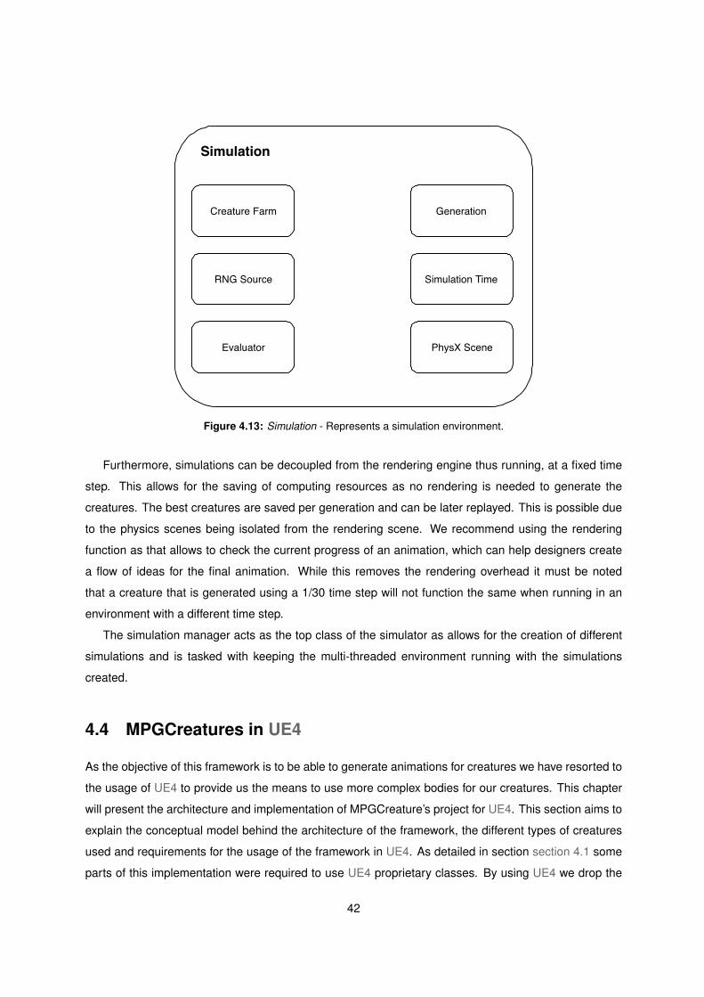
Creature Farm

Simulation

RNG Source

Evaluator

Generation

Simulation Time

PhysX Scene

Figure 4.13: Simulation - Represents a simulation environment.

Furthermore, simulations can be decoupled from the rendering engine thus running, at a fixed time

step. This allows for the saving of computing resources as no rendering is needed to generate the

creatures. The best creatures are saved per generation and can be later replayed. This is possible due

to the physics scenes being isolated from the rendering scene. We recommend using the rendering

function as that allows to check the current progress of an animation, which can help designers create

a flow of ideas for the final animation. While this removes the rendering overhead it must be noted

that a creature that is generated using a 1/30 time step will not function the same when running in an

environment with a different time step.

The simulation manager acts as the top class of the simulator as allows for the creation of different

simulations and is tasked with keeping the multi-threaded environment running with the simulations

created.

4.4 MPGCreatures in UE4

As the objective of this framework is to be able to generate animations for creatures we have resorted to

the usage of UE4 to provide us the means to use more complex bodies for our creatures. This chapter

will present the architecture and implementation of MPGCreature’s project for UE4. This section aims to

explain the conceptual model behind the architecture of the framework, the different types of creatures

used and requirements for the usage of the framework in UE4. As detailed in section section 4.1 some

parts of this implementation were required to use UE4 proprietary classes. By using UE4 we drop the

42

simulation manager from the previous simulator as parallelization can now be achieved by adding more

creatures in the same level.

4.4.1 Architecture

Most of the architecture conceptual model and implementation originate from section 4.3, however

changes were done to ensure full compability and ease of use with UE4, as can be seen in Figure 4.14.

SkeletalCreature

The first type of creature and probably the most complex and widely used in the creation process of game

assets, normally created using modelling tools. The conceptual model of this creature is very similar

to the creature used in the simulator, present in section 4.3 replacing the body with a SkeletalMesh,

a component in UE4 that is the composition of a mesh and a skeleton that can be animated. This

component contains the information about the skeleton such as bone names and gives us access to

the state of each bone in terms of orientation and position. A SkeletalMesh also contains the physics

constraints, or joints, created between bones which are required for the physics simulation. By using

UE4 we have different built-in options for the actuation of the creatures. While possible to add torque to

a joint location, we have opted to use angular drives to drive the joints of our creatures as it produces

more realistic and controllable behavior than adding torque as we can use the NN outputs as values

defining a desirable orientation and a desirable velocity to reach that orientation and the physics engine

calculates the needed force to apply to each joint.

Skeletal Creature

SkeletalMesh

Organism

MeasuredFitness

Starting Position

NumberOfSensors

NumberOfHidden

NumberOfOutputs

JointConstraints

Figure 4.15: SkeletalCreature - the new creature architecture.

The number of nodes for each layer of the NN can also be set and read from the creature as each

creature keeps a record of those values. Upon instantiating a creature, these numbers are automatically

loaded with the number of inputs being defined by the user, the number of outputs being automatically

43

Genome Manager

Creates Generation

Genomes

Creature Farm

Creatures

Assign organismto body

Passed to farm

LevelPhysics Simulation

Creatures tested in thesimulation

Evaluator

Creatures evaluatedaccording to task

RequestNext

Generation

Simulation

RequestNext

Generation

NEATAnim

UE4

Figure 4.14: MPGCreatures in UE4 - The main conceptual model is very similar to the simulator. Most of theclasses are now run inside UE4 with minimal differences that allow for the functionality to be extendedto the blueprint system of UE4 for easier use.

44

calculated using

#outputnodes = #joints ∗ 6 (4.1)

with #joints being automatically loaded from the skeleton and 6 representing the number of variables

we wish to use for each joint. The starting number of hidden nodes is recommended to be kept at 1 in

order to make use of the minimization propriety of NEAT as shown in section 3.4, even though AccNEAT

introduces the functionality of eliminating unnecessary nodes and links, starting from a minimal state is

desirable.

(a) Spider SkeletalMesh (b) Human SkeletalMesh

Figure 4.16: Two different skeletal meshes and their corresponding skeletons shown in white.

In order to control a creature we use the built-in angular motor provided by PhysX. We acknowledge

that there are better ways to control a creature in a physics simulation such as a muscle-based system

or with the use of PID controllers, but that is out of the focus of this work. A creature’s NN calculates

the output for the orientation and velocity to drive the angular motor, requiring three outputs for each

parameter, which calculates the necessary forces to rotate the joints of the skeleton. This allows for

better control of the force applied, instead of directly using torque to rotate the joints. It is possible to

limit the maximum degree of rotation for each angle in order to create more realistic movement and

behavior. In our case we have limited the rotations to 180 degrees, ranging from -90 to 90 for each axis.

An example of an initial neural network can be found in Figure 4.17.

45

Input

Hidden

Output Output Output Output Output Output

Figure 4.17: Example of an initial network- This network possesses a single input node and starts with the recom-mended number of hidden nodes, 1. This example network is a simplified version for just a single jointcreature. For a creature with more joints the network input and hidden layers would stay the same butthe output nodes would be N*6 where N is the number of joints. The network starts with the hiddennode connected to all output nodes.

SkeletalNoMeshCreature

A SkeletalNoMeshCreature is very similar to a SkeletalCreature but is simpler in terms of body topology.

As the name indicates, instead of a SkeletalMesh component, this type of creature is built using simple

static meshes, cubes, and physical constraints between those static meshes thus having no singular

mesh. As observable in Figure 4.18 the rest of the creature’s composition is very similar to a Skeletal-

Creature.While not as widely used, this type of creature enables the fast prototyping and usage of our

framework as simpler creatures are also easier for a NN to control, thus allowing for simpler and faster

simulations which are still able to demonstrate certain behaviors and motions such as getting up.

SkeletalNoMeshCreature

StaticMeshes

Organism

MeasuredFitness

Starting Position

NumberOfSensors

NumberOfHidden

NumberOfOutputs

JointConstraints

Figure 4.18: SkeletalNoMeshCreature - Similar to Figure 4.15 but using static meshes as body parts instead of amesh and a skeleton.

It is possible to create any type of body topology using the built-in editor in UE4, two examples can

46

be found in Figure 4.19. The configuration for the number of nodes of each type is also the same, with

constraints and network being automatically loaded.

(a) Quad Bot (b) Spider Bot

Figure 4.19: Two different topologies of SkeletalNoMeshCreature with their joints visible between static meshes.

Evaluators

While the evaluator functionality remains the same as the one presented in section 4.3, there was a

need to have fine-grained control over the evolution of creatures, as this is typical for real-time graphics

application where the method to reach our desired task matters, and thus we introduce the use of the

Tick method that is ran by UE4 at each frame. For tasks such as motion and movement, it is not enough

to look at the start and end of the simulation and exclude everything that happens in between and as

such we altered the original evaluator interface to expose a new method. The method Tick(DeltaTime,

Creatures), which is based on the Tick system of Unreal Engine, allows for an evaluation as precise

as a single frame time, allowing for the rewarding of a creature’s behavior in every simulation time step.

For example a creature learning how to stand might be able to stand but lose balance before the ending

of the simulation. Being rewarded only at the end of the simulation would mean that it would get a low

value for fitness even though the combination of nodes in the network of this creature was able to make

it stand but not keep balance until the end of the simulation. This helps with evolution as it allows us to

reward organisms that are closer to the goal but do not complete it.

4.4.2 Setting up creatures and levels

Creating a new creature with our framework is straightforward. By creating a new blueprint class that

inherits from the SkeletalCreature class as shown in Figure 4.20 and adding a Skeletal Mesh component

to it as presented in Figure 4.21 and selecting the corresponding mesh to be used, in this case a spider.

47

Figure 4.20: Creating a new creature - To create a blueprint class to use the framework it should inherit from theSkeletalCreature class provided.

Figure 4.21: Adding the skeletal mesh - To create a blueprint class to use the framework it should inherit from theSkeletalCreature class provided.

After creating the creature one should add the creature farm to the scene and indicate the creature

blueprint that the farm should use for the evolution. This step is needed to indicate to the creature farm

which creature should be respawned upon each new generation. The other configurable parameters can

be found in Figure 4.22 and these control the number of nodes for each layer of the initial neural network,

the training time in seconds and the number of creatures. The number of creatures is automatically

loaded by adding the tag "Training" to a creature placed in the scene.

48

Figure 4.22: Creature Farm Settings - This parameters indicate the current number of creatures in a scene, thenumber of nodes for each layer of the initial genome, the training time in seconds and the creatureblueprint to be used for the evolution process.

4.4.3 Concluding Remarks

In this chapter we have introduced the conceptual model of our framework and its components. We

started by introducing the NEATAnim package and the changes introduced when compared to the

AccNEAT package. We also introduced the PhysX Simulator were we can use simpler types of crea-

tures, in our case cubes, to learn how to solve tasks such as finding the solution to walking the most

distance in a single direction. Most of the components of the conceptual model are re-used as it is

possible to see in Figure 4.5 and Figure 4.14 where the conceptual model and idea is similar. Finally we

introduced the final framework that uses UE4 as the engine to power the level creation, rendering and

ability to use more complex types of bodies for our creatures along with the changes from the previous

simulator and how to use the framework inside the engine.

49

5Evaluation

Contents

5.1 Evaluation methodology . . . . . . . . . . . . . . . . . . . . . . . . . . . . . . . . . . . 53

5.2 Tests . . . . . . . . . . . . . . . . . . . . . . . . . . . . . . . . . . . . . . . . . . . . . . 53

51

This chapter will start by explaining the methodology and conditions used for the testing of the frame-

work in section 5.1. section 5.2 will describe the tests executed with the different types of creatures and

the setup taken for each test as well as discuss the results for each of the tests.

5.1 Evaluation methodology

This section presents the testing conditions and evaluation methodology used. Unless otherwise stated

the tests were run on a machine with 4 cores and 4 threads, with NEATAnim configured to use 3 of

those threads. For the tests we have decided to create 1 scene in our standalone application and 4

different scenes in UE4 with different creatures: a human character, a spider character, a quadruped

bot and a spider bot, with the first two belonging to the SkeletalCreature type of creature while the last

two belong to the SkeletalNoMeshCreature type. Different tasks were used for each type of creature

in order to explore different types of behaviour that can emerge from the creatures. Each type of test

may have different types of creatures, this was done to ensure that the load of the physics system was

similar between each different test but can be changed to accelerate the learning process depending on

the available computational power.

5.2 Tests

5.2.1 Cubes

We have used the simulator, presented in section 4.3 to generate some preliminary results. We have

designed an obstacle course and have tasked the cubes with arriving to a certain point in the scene.

This evaluator uses two different formulae, for attributing fitness to a creature, based on distance to the

center of the target circle. If the creature is outside of a predefined range of the circle, the fitness is given

by

CreatureF itness = CreatureF itness+ 100/distance (5.1)

where distance is the delta between the square distance to the center of the target and the square

of the predefined range.

If a creature is inside the range the fitness is calculated using

CreatureF itness = CreatureF itness+ (1− v) ∗ 100 (5.2)

and v is calculated using

53

Eye X Y Z W Walk

Hidden

Out.X Out.Y Out.Z

Bias

Figure 5.1: Initial genome setup - The genome starts with a bias node set to the fixed value of 1. It contains 6 inputsensor nodes that use the value from the eye sensor, the orientation sensor and the walk sensor.

v = d/(range) (5.3)

where d is the distance to the center of the target. In sum, the formula attributes fitness, depending if

they are inside the range, or not, of the circle by calculating, if outside the circle, the distance to the circle

itself, and if inside the circle, the distance to the center of the circle. To note that creatures that reach the

circle also receive a flat 100 fitness bonus to help guide evolution. The population for this test has 100

cube creatures, with the initial genome starting with 1 bias node set to 1, 6 input nodes, where 1 input

node is dedicated to receiving the values from the eye sensor, a sensor that outputs the distance to an

object by tracing a ray with a range of 50 units in the x axis, 4 input nodes are dedicated to receive the

quaternion values that give the current orientation of the cube and the last input node is a fixed value of

1. The number of hidden nodes is set to 1, as recommended, while the number of output nodes is set to

3 and the output values are used as the variables to be applied as torque in the 3 axis. This can be seen

in Figure 5.1 Simulation time for this test was set at 30 seconds, to give enough time for creatures to be

able to reach the circle, due to the distance between the starting position and the target. This scene can

be seen in Figure 5.3.

The test was successfully completed in 28 generations with the final genome having a fitness score

of 113.47 with 14 links and the same 11 nodes that it started with, meaning that to solve this problem,

the genome only created new links, in total it created 4 new links, and changed the weights of the links.

The successful run of this test was a preliminary step in making sure that the both our computational

model and the use of NE is possible in 3D real-time applications and that it can be used to solve tasks

in a virtual world.

54

Eye X Y Z W Walk

Hidden

Out.X Out.Y Out.Z

Bias

Figure 5.2: Solution genome - The final genome contains the same nodes but has new connection links betweennodes, including recurrent connections. It has ended with a total of 14 links from an initial 10. The newlinks are marked in red.

Figure 5.3: The obstacle course test - Creatures start at the center of the scene where the axis is marked andhave the task of reaching the blue circle on the right of the obstacles. The cube creatures are coloredin green when moving and dark green when inactive. Obstacles are shown in light blue.

55

Figure 5.4: A creature solving the task - At the 28th generation mark a cube was able to dodge the obstacles andreach the center point. Obstacles are shown in light blue while the cube that solved the task is coloredin red.

5.2.2 Walking spiders

The first test in UE4 presented is to evolve spiders to walk in a certain direction. This test is setup with

a level without obstacles. 84 spiders were placed in a plane. The evaluator used is analysing the scene

per frame and attributing a value of fitness equal to the delta distance walked in the positive X axis. This

evaluator promotes the constant movement of a creature by using the formula

CreatureF itness = CreatureF itness+ (CurrentPosition.X − LastPosition.X) ∗ TotalT ime (5.4)

which attributes more points the more time has passed and the higher the delta between each frame.

The scene is setup as seen in Figure 5.5. The spiders have 10 joint constraints which the neural

networks can control. This test was executed with an initial genome with 31 input nodes, with 1 input

node for a walking sensor and 3 input nodes for each joint as we use an orientation sensor per joint so

that the network can have knowledge of the state of each joint of the body, 1 hidden node and 60 output

nodes. We have also limited the angular motion to 45 degrees in each axis. The angular motor is set

with a strength of 4000 as it offered a good balance between bone rigidity and realistic control. This

value was reached through trial and error as initially the creature’s members were too fragile to sustain

the spider’s body and too high of a value makes the movements to become too stiff and looking more

robotic.

56

Figure 5.5: Spider Test Scene - The scene is composed of 4 walls, a plane and 84 spider creatures.

(a) Spider Physics Primitives (b) Angular Motor Settings

Figure 5.6: The physics body and angular motor settings used for this test.

The simulation time was set to 10 seconds and some example results can be found in Figure 5.7.

With this configuration, the evolution process between generations has an average execution time of

65.52 milliseconds.

After 194 generations behavior that resembles a struggling spider to walk started emerging. At the

57

407th generation mark, spiders were walking a few steps while acting drunkenly1 This was achieved

without feeding any information for any type of animation.

While spiders were able to walk in the correct direction, there were subtle differences between dif-

ferent species of genomes. This is easily observable in the still images 5.7(b) and 5.7(c) where we can

see that for the same time step different spiders are using different legs to promote their movement.

5.2.3 Human character raising an arm

The second test of our framework takes the form of human characters. This test uses the skeletal mesh

presented in 4.16(b) and uses a hybrid between physics simulation and kinematic animation. Instead

of allowing the neural network to take control of the whole body, we only let the neural network to take

control of a certain member of the body, a member that is set to simulate physics. In this test we decided

to make a character raise their hand while the rest of body stands still. For this we set all the bones

below, and including, the upper arm bone, shown as the orange bone in Figure 5.8.

Figure 5.8: The upper arm bone - Every bone below, in the hierarchy, the one marked as orange will be simulatingphysics for this test.

The initial genome construction is similar to the one presented in subsection 5.2.2 with 3 input nodes

for each of the 3 joints, that connect the arm to the lower arm and hand, and 1 input node that represents

if the animation should be played or not, totalling 10 input nodes. The hidden layer consists of 1 node.

The output layer has 6 nodes for each controllable joint totalling 18 output nodes.

1Video footage of the evolution process for walking spiders available at https://www.youtube.com/watch?v=0Ilf0wv2VoQ, lastseen 09/10/2019.

58

(a) Initial Positions

(b) Going Forward

(c) Still 3

(d) Still 4

Figure 5.7: Still images captured on generation 410 of the evolution process.

59

The formula used to evaluate the performance of a genome and guide the evolution,

CreatureF itness = CreatureF itness+RightHand.Z ∗ TotalT ime (5.5)

uses the Z axis position, which for UE4 is considered the default world up vector, of the hand that

should be raised as a metric of the performance of the network. The higher the hand is at a given

time, the more fitness the creature will accumulate, meaning that the NN controlling that creature is on

a good path to solve the task. More complex formulas could be used, taking into the account the delta

difference of the hand while it’s in the air. Results can be found in Figure 5.9. The human character

starts by rising the right arm up in a swift motion until the hand reaches the highest position with the

palm facing forwards. After reaching the highest position, the downwards motion starts and the character

rotates the arm and swings it down until it reaches rest position.

60

(a) (b) (c)

(d) (e) (f)

(g)


61

(a) Initial Positions (b) Starting to rise (c) Almost there (d) Standing up


5.2.4 Standing up Quad Bot

The third test and the first for SkeletalNoMeshCreatures. While this test uses the second type of crea-

tures introduced in section 4.4, the necessary setup is equal to the first two tests. We setup a level were

we placed 77 quad bots. We opted to use only one input node, a single 0 or 1, to be interpreted as a

go signal. This was done in order to reduce the input variation as using the joint orientation as an input

might create weird behavior if the physics simulation is not deterministic or has deviations between runs,

1 hidden node and 48 output nodes as we have 8 joints, divided between hip joints, that connect the

upper part of the legs to the central body, and knee joints, that connect the upper leg to the bottom leg

part. Simulation time was set to 5 seconds. The evaluator for this test takes the form of

CreatureF itness = CreatureF itness+BodyPosition.Z ∗ TotalT ime (5.6)

where the Z position of the body is used as the heuristic. Using the body’s position and the total time

elapsed during the simulation run allows to avoid weird corner cases where a creature might jump or not

fully extend and keep its balance but still get an high fitness if at the moment the simulation generation

ends, the creature’s body was somehow in a high position. This is a prime example of the need for per-

frame evaluators for this kind of task. By using this formula the fitness is maximized if a creature raises

as soon as possible and is able to keep its body at the maximum height possible for the longest period

of time. Due to the more simplistic nature of the creature’s body and of the task, it is expected that the

number of generations is lower than the test presented in subsection 5.2.2. With only 30 generations,

quad bots were able to stand up and keep balance as seen in 5.10(d).

The use of NE allows for the emergence of different behaviors for the same creature and body and

62

allows for the generation of different types of animation with the same objective yielding results that,

while similar, behave in different ways in order to solve the task proposed.

(a) (b) (c)

Figure 5.11: Different behaviors achieved during the same simulation.

Three examples of different creatures maintaining balance while standing up are shown in Fig-

ure 5.11 where 3 creatures can be seen posing in different ways2. These creatures were all generated

in the same simulation run, so in one run we were able to generate at least three animations for this

creature to get up from the floor.

5.2.5 Standing Spider Bot

The last test uses the creature shown in 4.19(b), which consists of a body and 8 legs. This test aims to

show how a creature with a different topology evolves when using the same evaluator as the one used

for the evolution of the quad bot and as such the evaluator formula is the same as shown in Equation 5.6.

The initial genome for this creature has 1 input node, 1 hidden node and 96 output nodes, containing 8

knee joints and 8 hip joints. As seen in Figure 5.12 the creature’s method to raise up uses most the legs

to propel the body up and is somewhat similar to the same starting pose when compared to the quad

bot. After raising up the creature uses 4 legs to balance the body. Finally, the creature is fully stabilized

using only 4 legs, with the remaining 4 legs being available to be explored as other options that are not

locomotion by the designer. This available arms could then be used as, e.g. weapons, robotic arms or

other creative idea that the designer thinks would suit the theme of the scene while keeping the creature

2Video footage of the evolution process for quad bots standing up available at https://youtu.be/hm2P1Mt3ZQo, last visised on23/10/2019.

63

(a) (b) (c) (d)


physically correct according to the world conditions, that is, that it can maintain balance, using only 4 of

the legs, while standing up with the remaining legs to be freely used as wished.

This shows that the same evaluator can produce different but accurate results in different creature

body topologies, allowing for the re-use of evaluators.

5.2.6 Discussion

In this chapter we have presented our tests and results. First we started by doing a preliminary test that

the usage of NE in real-time graphics applications was possible and we successfully generated cubes

that could solve an obstacle course. In the second test where we aimed to make a spider walk, we

were successful in creating walking spiders that could walk for a certain period of time as seen in the

provided footage. In the third test we wanted to test how our framework adapted not only to a different

body topology but also to restricted parts of a body, where our framework has provided interesting and

positive results in the creation of animation for the human character. Finally, our last two tests have

shown that not only can our framework adapt to different body topologies and methods of construction

but that the same evaluators can be re-used for different body topologies with interesting results, showing

that NE paired with neural networks is able to provide interesting motion and behavior for any kind of

body topology as it learns how to handle the body at hand.

64

6Conclusion

Contents

6.1 System Limitations and Future Work . . . . . . . . . . . . . . . . . . . . . . . . . . . . 68

65

We started this thesis by describing the importance of animation and variety in animation when hav-

ing multiple creatures that look the same but act slightly differently making a game more believable. We

have also described how the increase of complexity present in games and that the need for new anima-

tion for assets affects the costs of production and puts pressure on the animators that are tasked with

creating animations for a whole different range of characters for which they do not have the opportunities

to explore different possibilities. We have stated that our primary focus was to create a tool that could

aid in the creative process of creating animations where a designer, developer or animator could state

their task, e.g standing up or waving, in which the creature would take the environment and physical

conditions into account without having any data set of animation information, that is, using neuroevolu-

tion, which couples Genetic Algorithm (GA) with neural networks and uses an evolutionary process to

learn how to solve a task.

We have developed NEATAnim, a port of AccNEAT, a linux implementation of NEAT, aimed to work

in the Windows operative system in which we have further improved the ability of AccNEAT to work in

multiple parallel environments. This ability enables for multiple scenes to be simulated with different

tasks or parameterization without affecting each other.

A prototype simulator has been developed and presented with the main conceptual model being

reused for the final implementation of the project. In the final implementation we have created a frame-

work that can be used in UE4. This framework can be used to create tasks and new creatures in an

easy way with flexibility in the parameterization. By supplying the evaluator method it is possible to guide

the evolution towards the goal we want, e.g. walking in a direction, solving a obstacle course or standing

up, which have been tested and presented.

Finally, we have created a set of 5 tests in order to evaluate the performance of our framework in

creating animations. These tests differed in both creature topology and actions. The first test used cubes

in the simulator and an obstacle course which they had to solve to reach a point. This test worked as a

preliminary way of knowing if our computational model and framework would be able to create motion

guided by a goal. The second test used the most complex creature and managed to create spiders that

could walk, briefly, in one direction while maintaining their body in an upper position. The third test used

a human character that only simulated the right arm. The objective of this test was to demonstrate that

the framework is not limited to learning how to control the whole body, but that it can control a part of the

body while the remaining parts can remain in kinematic mode. The fourth and fifth tests demonstrated

that evaluators can be re-used between different creatures topologies with similar results, showing that

the creature’s NN does indeed learn how to control the creature’s body. All of the animations in the tests

were generated using PhysX’s angular drives and interaction with the plane on which they were set, thus

making them fully physically-based as was hypothesized.

67

6.1 System Limitations and Future Work

There are still some issues that need exploring and addressing in terms of reproducibility.

Currently UE4 and PhysX have some issues with replaying the simulated results. While there’s a

way to replay a solution, as we do export and import successfully the resulting neural networks that

were successful in the simulation, since the time step and frame rate are variable, there are issues

where the animation might break due to miscalculations in the physics engine. A possible way to solve

this issue is to save the transforms for each bone of a skeleton and create a kinematic animation from

those values. This would solve the problem of not being able to accurately replay the animation as

we could decouple the generated animation, using physics simulation, from the actual physics engine

when playing. That is, convert the physics simulation, as executed in the simulation, into a kinematic

animation. This also has the bonus of being less resource intensive.

A better physics actuator system and a converter can be developed, that can take the simulated

animation to a kinematic animation by recording the bone transforms, per frame, into a buffer, and

later reusing those transforms in a kinematic way would greatly improve the usage of the animations

generated directly in an application for further editing by the designer.

After having such an intermediary converter, running user tests with animation designers or game

developers becomes easier, as evolutionary animation is a different paradigm compared to the current

state of animation development.

Another issue is the subjectivity of animation and of the creative process. Creating and designing

animations for characters is an highly complex process where designer input can affect the emotion and

personality transmitted by the character, making an automated process harder to generate a complete

animation that is ready to use.

Another interesting approach would be to explore new tasks using a neural network that has been

trained before for a previous task, e.g. waving after standing up, where the initial network has already

learned how to stand up, to check if the previous behavior learned is still present after further evolution.

68

Bibliography

[1] J. Togelius, N. Shaker, and M. J. Nelson, “Introduction,” in Procedural Content Generation in

Games: A Textbook and an Overview of Current Research, N. Shaker, J. Togelius, and M. J.

Nelson, Eds. Springer, 2016, pp. 1–15.

[2] C. Hecker, B. Raabe, R. W. Enslow, J. DeWeese, J. Maynard, and K. van Prooijen, “Real-time

motion retargeting to highly varied user-created morphologies,” ACM Transactions on Graphics,

vol. 27, no. 3, p. 1, 2008. [Online]. Available: http://portal.acm.org/citation.cfm?doid=1360612.

1360626

[3] A. Beane, 3D animation essentials. Sybex Incorporated, 2012.

[4] Katherine Pullen and Christoph Bregler, “Motion capture assisted animation: Texturing and synthe-

sis.” ACM Transactions on Graphics, vol. 21, no. 3, pp. 501–508, 2002.

[5] V. B. Zordan and J. K. Hodgins, “Motion capture-driven simulations that hit and react,” Proceedings

of the 2002 ACM SIGGRAPH/Eurographics symposium on Computer animation - SCA ’02, p. 89,

2002. [Online]. Available: http://portal.acm.org/citation.cfm?doid=545261.545276

[6] A. Dasgupta and Y. Nakamura, “Making Feasible Walking Motion of Humanoid Robots From Hu-

man Motion Capture Data,” Proceedings of the 1999 IEEE International Conference on Robotics &

Automation, vol. 2, no. May, pp. 1044–1049, 1999.

[7] A. Aristidou, J. Lasenby, Y. Chrysanthou, and A. Shamir, “Inverse Kinematics Techniques in Com-

puter Graphics: A Survey,” Computer Graphics Forum, vol. 37, no. 6, pp. 35–58, 2018.

[8] T. Komura, E. S. Ho, and R. W. Lau, “Animating reactive motion using momentum-based inverse

kinematics,” Computer Animation and Virtual Worlds, vol. 16, no. 3-4, pp. 213–223, 2005.

[9] M. Neff, “Modeling Tension and Relaxation for Computer Animation,” Proceedings of the 2002 ACM

SIGGRAPH/Eurographics symposium on Computer animation, pp. 81–88, 2002.

[10] T. Geijtenbeek and N. Pronost, “Interactive Character Animation using Simulated Physics,” Com-

puter Graphics Forum, vol. 31, no. 8, pp. 2492–1, 2012.

69

http://portal.acm.org/citation.cfm?doid=1360612.1360626



[11] W. Armstrong and M. Green, “The dynamics of articulated rigid bodies for purposes of animation,”

The Visual Computer, vol. 1, no. 4, pp. 231–240, 1985.

[12] P. Hong, Z. Wen, T. S. Huang, and L. Fellow, “Real-Time Speech-Driven Face Animation With

Expressions Using Neural Networks,” IEEE Transactions on Neural Networks, vol. 13, no. 4, pp.

916–927, 2002.

[13] R. Grzeszczuk and G. Hinton, “NeuroAnimator: Fast Neural Network Emulation and Control of

Physics-Based Models,” Proceedings of SIGGRAPH 98, 1998.

[14] T. Reil and P. Husbands, “Evolution of central pattern generators for bipedal walking in a real-time

physics environment,” IEEE Transactions on Evolutionary Computation, vol. 6, no. 2, pp. 159–168,

2002.

[15] F. Amato, A. Lopez, E. M. Pena-Mendez, P. Vanhara, A. Hampl, and J. Havel, “Artificial neural

networks in medical diagnosis,” Journal of Applied Biomedicine, vol. 11, no. 2, pp. 47–58, 2013.

[16] M. Plagge, “Using artificial neural networks to predict first-year traditional students second year

retention rates,” Proceedings of the 51st ACM Southeast Conference on - ACMSE ’13, p. 1,

2013. [Online]. Available: http://www.scopus.com/inward/record.url?eid=2-s2.0-84881650482&

partnerID=tZOtx3y1

[17] R. Wang and Z. Xu, “A pedestrian and vehicle rapid identification model based on

convolutional neural network,” Proceedings of the 7th International Conference on Internet

Multimedia Computing and Service - ICIMCS ’15, pp. 1–4, 2015. [Online]. Available:

http://dl.acm.org/citation.cfm?doid=2808492.2808524

[18] K. O. Stanley, “Neuroevolution: A different kind of deep learning,” O’Reilly, 2017. [Online].

Available: https://www.oreilly.com/ideas/neuroevolution-a-different-kind-of-deep-learning

[19] X. Yao, “Evolving Artificial Neural Networks,” Proceedings of the IEEE, vol. 87, no. 9, 1999. [Online].

Available: https://pdfs.semanticscholar.org/6fff/fbd6a689aea053242b86a19b78dc5934fee9.pdf

[20] Felix Streichert, “Introduction to Evolutionary Algorithms,” Evolutionary Algorithms in Molecular De-

sign, vol. 8, pp. 1–13, 2008.

[21] M. Mitchell, An Introduction to Genetic Algorithms. Cambridge, MA, USA: MIT Press, 1998.

[22] D. Holden, T. Komura, and J. Saito, “Phase-functioned neural networks for character

control,” ACM Transactions on Graphics, vol. 36, no. 4, pp. 1–13, 2017. [Online]. Available:


70

http://www.scopus.com/inward/record.url?eid=2-s2.0-84881650482&partnerID=tZOtx3y1

http://www.scopus.com/inward/record.url?eid=2-s2.0-84881650482&partnerID=tZOtx3y1


https://www.oreilly.com/ideas/neuroevolution-a-different-kind-of-deep-learning

https://pdfs.semanticscholar.org/6fff/fbd6a689aea053242b86a19b78dc5934fee9.pdf


[23] H. Zhang, S. Starke, T. Komura, and J. Saito, “Mode-adaptive neural networks for quadruped

motion control,” ACM Transactions on Graphics, vol. 37, no. 4, pp. 1–11, 2018. [Online]. Available:


[24] K. Sims, “Evolving virtual creatures,” Proceedings of the 21st annual conference on Computer

graphics and interactive techniques - SIGGRAPH ’94, vol. 4, no. 1, pp. 15–22, 1994. [Online].

Available: http://portal.acm.org/citation.cfm?doid=192161.192167

[25] K. O. Stanley and R. Miikkulainen, “Evolving neural networks through augmenting topologies,”

Evolutionary Computation, vol. 10, no. 2, pp. 99–127, 2002. [Online]. Available: https:

//www.mitpressjournals.org/doi/10.1162/106365602320169811

[26] E. Haasdijk, A. A. Rusu, and A. E. Eiben, “HyperNEAT for locomotion control in modular robots,”

Lecture Notes in Computer Science (including subseries Lecture Notes in Artificial Intelligence and

Lecture Notes in Bioinformatics), vol. 6274 LNCS, pp. 169–180, 2010.

[27] L. Cardamone, D. Loiacono, and P. L. Lanzi, “Evolving competitive car controllers for

racing games with neuroevolution,” Proceedings of the 11th Annual conference on Genetic

and evolutionary computation - GECCO ’09, pp. 1179–1186, 2009. [Online]. Available:


[28] E. Hastings, R. Guha, and K. O. Stanley, “NEAT particles: Design, representation, and animation of

particle system effects,” Proceedings of the 2007 IEEE Symposium on Computational Intelligence

and Games, CIG 2007, pp. 154–160, 2007.

[29] D. James and P. Tucker, “A Comparative Analysis of Simplification and Complexification

in the Evolution of Neural Network Topologies [late breaking paper],” The 6th Annual

Conference on Genetic and Evolutionary Computation - GECCO ’04 (Seattle, WA), 2004.

[Online]. Available: http://anji.sourceforge.net/docs/james gecco04.pdf%5Cnftp://ftp.cs.bham.ac.

uk/.snapshot/hourly.0/pub/authors/W.B.Langdon/biblio/gecco2004/LBP019.pdf

71



https://www.mitpressjournals.org/doi/10.1162/106365602320169811

https://www.mitpressjournals.org/doi/10.1162/106365602320169811


http://anji.sourceforge.net/docs/james_gecco04.pdf%5Cnftp://ftp.cs.bham.ac.uk/.snapshot/hourly.0/pub/authors/W.B.Langdon/biblio/gecco2004/LBP019.pdf

http://anji.sourceforge.net/docs/james_gecco04.pdf%5Cnftp://ftp.cs.bham.ac.uk/.snapshot/hourly.0/pub/authors/W.B.Langdon/biblio/gecco2004/LBP019.pdf

AAppendix A

Classes

Below we present an itemized list of the base classes present in NEATAnim and their functionalities.

• Genome - Contains node and link information, i.e. the genotype

• Network - The actual instanciated NN, i.e. the phenotype

• Organism Evaluation - Keeps track of the evaluation of an Organism

• Organism - Combination of a genome and the corresponding network together with the fitness

value

• Genome Manager - Handles the crossover and mutation of genomes

• Species - Group of genomes that are compatible with each other according to Equation 3.1

• Population - The whole population separated into species

• Innovation - Keeps track of the genetic innovations to be applied at the end of the generation

73

• NeatENV - Global struct that keeps the parameters used by the algorithm

• Evaluator - Stipulates and evaluates the genomes according to a task

• Experiment - represents a task to be executed, e.g. the XOR test

Listing A.1: Example of an eye sensor’s get activations() method.

1

2 std::map<unsigned int, float>& EyeSensor::get activations()

3 {

4 PxVec3 origin = this->body->getGlobalPose().p + PxVec3(2.5,0,0);

5 PxRaycastBuffer hit;

6 PxQueryFilterData filterData = PxQueryFilterData();

7 filterData.data.word0 = FilterData::eOBSTACLE;

8 bool status = scene->raycast(origin, this->dir,

9 this->range, hit, PxHitFlag::eDEFAULT, filterData);

10 if (status) {

11 this->activations[idx] = 1 - ((1 - 0)*((hit.block.distance - 0)) / (this->range - 0));

12 }

13 else

14 this->activations[idx] = 0.0;

15

16 return this->activations;

17 }

74

mixed procedurally generated creatures

Documents