mit phd international trade 25: trade...

14.581 MIT PhD International Trade – Lecture 25: Trade Policy (Theory) –

Dave Donaldson

Spring 2011

1

2

1

3

1

4

1

5

Today’s Plan

Introduction to the study of trade policy.

The traditional economic approach (welfare-maximizing trade policy).

Johnson (1954) via Bagwell and Staiger (1999).

The political-economy approach (government not necessarilywelfare-maximizing).

Grossman and Helpman (1994).

Rationalizing trade agreements.

Bagwell and Staiger (1999).

Other topics in the study of trade policy.

1

2

1

2

3

Trade Policy Literature A Brief Overview

• Key questions: Why are countries protectionist? Can protectionism ever be “optimal”? Can we explain how trade policies vary across countries, industries, and time?

How should trade agreements be designed? Can we explain the main institutional features of actual trade agreements (e.g. WTO, NAFTA, EU)?

• In order to shed light on these questions, one needs to take a stand on the:

Economic environment: What is the market structure? Are there distortions, e.g. unemployment or pollution?

Political environment: What is the objective function that governments aim to maximize, e.g. social welfare, welfare of the median voter, political support? What are the trade policy instruments, e.g. import tariffs, quotas, product standards? Are trade policy instruments the only instruments available?

Constraints on the set of feasible contracts: Do trade agreements need to be self-enforcing? How costly is it "to complete” contracts?

1

2

1

2

1

2

This Lecture

We will restrict ourselves to economic environments such that: •

All markets are perfectly competitive.

There are no distortions.

• We will be focusing on two questions:

How should tariffs vary across countries and industries?

What is the rationale for trade agreements?

• Our goal will be to contrast the implications of two assumptions:

Governments only care about welfare [the “Traditional economic approach”.]

Governments are politically motivated [the “Political Economy apprach”, where we will focus in particular on the work of Grossman and Helpman (1994).]

1

2

1

3

1

4

1

5

Today’s Plan


The traditional economic approach (welfare-maximizing trade policy). Johnson (1954) via Bagwell and Staiger (1999).






Economic Environment

• Consider a world economy with 2 countries, c = 1, 2.

• There are two goods, i = 1, 2, both produced under perfect competition.

• Good 2 is used as the numeraire, p2 w = 1.

Notations:•

pc ≡ p1 c /pc is the relative price in country c .• 2

pw ≡ p1 w /pw is the “world” (i.e. pre-tax) relative price.• 2

dc (pc , pw ) is the demand for good i in country c .• i

y c (pc ) is supply of good i in country c• i

� � � �

� � � �

� � � �

� � � �

� � � �

� � � �

� � � �

Economic Environment (Cont.)

• WLOG, country 1 (resp. 2) is a natural importer of good 1 (resp. 2):

m11 p1 , pw ≡ d1

1(p1 , pw ) − y11 p1 > 0

m22 p2 , pw ≡ d2

2(p2 , pw ) − y22 p2 > 0

x1 p1 , pw ≡ y21 (p1 ) − d1 p1 , pw > 02 2

x12 p2 , pw ≡ y1

2 (p2 ) − d12 p2 , pw > 0

Trade is balanced: •

w 1 1 w 1 1 wp m1 p , p = x2 p , p

2 2 w w 2 2 wm2 p , p = p x1 p , p

• Market clearing for good 2 requires:

x21 p1 , pw = m2

2 p2 , pw (1)

Political Environment Policy instruments

• Both governments can impose an ad-valorem tariff tc on their imports

pc c pw c = (1 + t ) c

pc w−c = p−c

• Tariffs create a wedge between the world and local prices which implies � p1 = 1 + t1

p2 pw / 1

� pw (2) � t2= +�

(3)

• Comments:• If the only taxes are import tariffs, then local prices faced by consumers and producers are the same, as implicitly assumed in our previous slides.

• Equations (1)-(3) implicitly define pw ≡ pw

�t1 , t2

�and pc ≡ pc (tc , pw )

Political Environment Government ’s objective function

• Both governments are welfare-maximizers. They simultaneously set tc in order to maximize utility of representative agent:

max V c (pc , I c ) ≡ V c [pc , Rc (pc ) + Tc (pc , pw )] (4)tc

where:

Rc (pc ) ≡ maxy {p1 c y1 + p2 c y2 |y feasible}

1 1 1 , pw � � � � � Tc (pc , pw ) ≡ tc pwmc (pc , pw ) = �p − pw m� p � if� c = 11

c c pw /p2 − 1 m22 p2 , pw if c = 2

p1 , p2 , pw satisfy Equations (1) − (3)

1

2

3

4

5� � � �

Unilateral Tariffs

• Proposition 1 For both countries, unilateral (Nash) tariffs satisfy

1 d ln x−c tc =

ε−c , where ε−c ≡

d ln pw

Proof: •

For expositional purposes we focus on country 1. FOC ⇒ � Vp 1 ��

dp1 � �

dR1 ��

dp1 �

V 1 dt1 +

dp1 dt1I

+ � dp1 ∂pw �

m11 � p1 , pw

� + t1pw dm1

1 � p1 , pw � = 0

dt1 −

∂t1 dt1

Roy’s identity Vp 1

= −d11 (p1 , pw )⇒ VI 1

Perfect competition dR 1 = y 1 1 , pw )⇒ dp1 � 1 (p �

1+2+3 ⇒ t1 = �

∂ ln ∂tp1

w �

/ d ln m1

1

dt(p1

1 ,pw )

4 + market clearing, m11 p1 , pw = x1

2 p2 , pw t1 = 1/ε2 ⇒

1

2

3

How Should Tariffs Vary Across Countries (and Industries)?

• Proposition 1 offers a simple positive theory of tariff formation:

• Tariffs≡ inverse of the elasticity of foreign export supply. • This is true whether or not the other government is imposing its Nash tariff. • Though other government’s tariff does affect elasticity of foreign export supply.

In the case of a small open economy, ∂pw = 0 ε2 = +∞•

∂t1 ⇒ • A small open economy never has an incentive to impose a tariff.

• According to traditional economic approach, import tariffs are intimately related to countries’market power.

• It is a country’s ability to improve its terms-of-trade that leads to strictly positive tariffs.

Potential concerns: •

Do we really believe that governments maximize welfare?

How many countries are “large” enough to affect their terms-of-trade?

Do trade negotiators really care about their terms-of-trade?

� �

� � � �

Are Unilateral Tariffs Pareto-Effi cient?

• Following Bagwell and Staiger (1999), we introduce

Wc (pc , pw ) ≡ V c [pc , Rc (pc ) + Tc (pc , pw )]

• Differentiating the previous expression we obtain � � � � �� dpc ∂pw ∂pw

dW c = Wpcc

dtc + Wp

cw

∂tc dtc + Wp

cw

∂t−c dt−c

• The slope of the iso-welfare curves can thus be expressed as

� � W 1 ∂pw

dt1 pw ∂t2

dt2 = �

dp1 � �

∂pw � (5)

dW 1 =0 Wp11 + Wp

1 w ∂t1dt1 � � W 2 dp2 + W 2 ∂pw

dt1 =

p2 dt2 � pw � ∂t2

(6)dt2 dW 2 =0 Wp

2 w

∂∂ptw

1

1

2

3

� � � �

� � � �

� � � �

� � � �

Are Unilateral Tariffs Pareto-Effi cient?

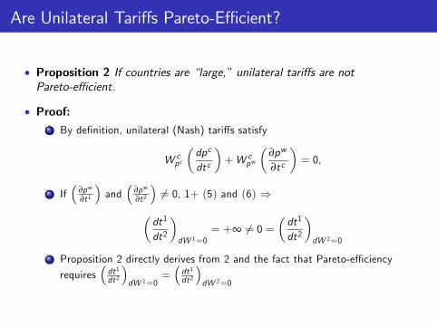
• Proposition 2 If countries are “large,” unilateral tariffs are not Pareto-effi cient.

Proof: •

By definition, unilateral (Nash) tariffs satisfy

Wpcc dpc

+ Wpcw

∂pw = 0,

dtc ∂tc

If ∂pw and ∂pw

= 0, 1+ (5) and (6)∂t1 ∂t2 � ⇒

dt1 dt1

dt2 dW 1 =0 = +∞ �= 0 =

dt2 dW 2 =0

Proposition 2 directly derives from 2 and the fact that Pareto-effi ciency

requires dt1 = dt1 dt2 dW 1 =0 dt2 dW 2 =0

Are Unilateral Tariffs Pareto-Effi cient? Graphical analysis (Johnson 1953 -54)

• N corresponds to the unilateral (Nash) tariffs

• E-E corresponds to the contract curve

• If countries are too asymmetric, free trade may not be on contract curve

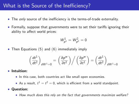
• The only source of the ineffi ciency is the terms-of-trade externality.

• Formally, suppose that governments were to set their tariffs ignoring their ability to affect world prices:

W 1p1 = W 2

p2 = 0

• Then Equations (5) and (6) immediately imply �dt1

dt2

� � ∂pw ∂pw dt1

= = t2 1

dW 1 =0 ∂

��∂t

� �dt2

�dW 1 =0

• Intuition:• In this case, both countries act like small open economies.

• As a result, t1 = t2 = 0, which is effi cient from a world standpoint.

• Question: • How much does this rely on the fact that governments maximize welfare?

What is the Source of the Ineffi ciency?

1

2

1

3

1

4

1

5

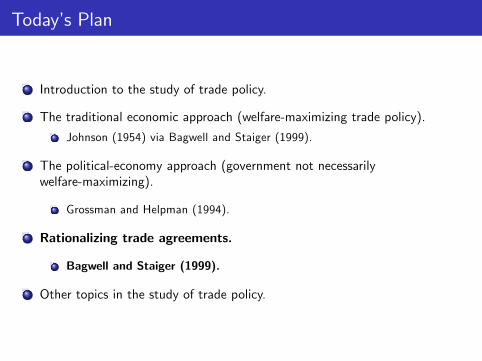
Today’s Plan




The political-economy approach (government not necessarily welfare-maximizing).





�

Economic Environment Endowment economy

• We consider a simplified version of Grossman and Helpman (1994).

• To abstract from terms-of-trade considerations, we consider a small open economy.

• There are n + 1 goods, i = 0, 1, ..., n, produced under perfect competition:

• Good 0 is a freely-traded numeraire with domestic and world price equal to 1.

• pw and pi denote the world and domestic price of i good i , respectively.

• Agents are endowed with one unit of good 0 and one unit of another good i = 0.

• We refer to an agent endowed with good i as an i -agent.

• αi denote the share of i -agents in the population.

• Total number of agents is normalized to 1

Economic Environment (Cont.) Quasi -linear preferences

• All agents have the same quasi-linear preferences:

U = x0 + ∑ni =1 ui (xi )

• Indirect utility function of i-agent is therefore given by:

Vi (p) = 1 + pi + t (p) + s (p)

where:

t (p) ≡ government’s transfer [to be specified]

s n n (p) ≡ ∑i=1 ui (di (pi )) − ∑i=1 pi (di (pi ))

• Comments:• Original GH (1994) model is a specific-factor model (not endowment model as here).

• Given quasi-linear preferences, this is de facto a partial equilibrium model

Political Environment Policy instruments

• For all goods i = 1, ..., n, the government can impose an ad-valorem import tariff/export subsidy ti

p i = 1 + t w( i ) pi

• We treat p ≡ (pi )i as the policy =1,...,n variables of our government.

• The associated government revenues are given by:

t p ∑n p − pw m p n w ( ) = i =1 ( i i ) i ( i ) = ∑i =1 (pi − pi ) [di (pi ) − αi ]

• Revenues are uniformly distributed to the population so that t (p) is also equal to the government’s transfer, as assumed before.

Political Environment Lobbies

• An exogenous set L of sectors/agents is politically organized.

• We refer to a group of agents that is politically organized as a lobby.

· + n• Each lobby i chooses a schedule of contribution Ci ( ) : (R ) +R in

order to maximize the total welfare of its members net of the contribution:→

max 0 0 αi Vi p − Ci pCi (·)

subject to: p0 = argmax

� �G (p)

� �p

where G (·) is the objective function of the government [to be specified], and αi relates to the ‘size/importance’of lobby i .

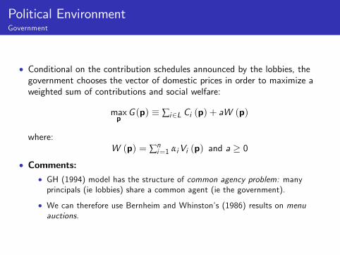
Political Environment Government

• Conditional on the contribution schedules announced by the lobbies, the government chooses the vector of domestic prices in order to maximize a weighted sum of contributions and social welfare:

max G (p) ≡ ∑i ∈L Ci (p) + aW (p)p

where:W (p) = ∑n

i =1 αi Vi (p) and a ≥ 0

• Comments:• GH (1994) model has the structure of common agency problem: many principals (ie lobbies) share a common agent (ie the government).

• We can therefore use Bernheim and Whinston’s (1986) results on menu auctions.

1

2

3

��

� � � �

� � � �

� � � �

Equilibrium Contributions

• We denote by Ci 0 i ∈L , p

0 the SPNE of the previous game.

• We restrict ourselves to interior equilibria with differentiable equilibrium contribution schedules.

• Whenever we say “in any SPNE”, we really mean “in any interior SPNE where C 0 is differentiable.”

• Lemma 1 In any SPNE, contribution schedules are locally truthful:

�C 0 p0 = αi �Vi p0 i

Proof: •

p0 optimal for the government ∑i ∈L �Ci 0 p0 + a�W p0 = 0.⇒

C 0 ( ) optimal for lobby ii · � � � � ⇒ � � � �αi �Vi p0 − Ci p0 + ∑i ∈L �C 0 p0 + a�W p0 = 0.� i �

1+2 ⇒ �Ci 0 p0 = αi �Vi p0 .

1

2

3

� �

� � � � � � � �

Equilibrium Trade Policies

• Lemma 2 In any SPNE, domestic prices satisfy:

∑ni =1 αi (Ii + a) �Vi p0 = 0,

where Ii = 1 if i is politically organized and Ii = 0 otherwise.

Proof: •

p0 optimal for the government ∑i ∈L �Ci 0 p0 + a�W p0 = 0.⇒

1 + Lemma 1 p0 p0 = 0.⇒ ∑i ∈L αi �Vi + a�W � � Lemma 2 directly derives from this observation and the definition of W p0 .

Comment:•

• In GH (1994), everything is as if governments were maximizing a social welfare function that weighs different members of society differently.

1

2

3

� �

� � • � �

� �

� � � �

Equilibrium Trade Policies (Cont.)

• Proposition 2 In any SPNE, trade policies satisfy

t0 z0 i = Ii − αL i

0 for i = 1, ..., n, (7)1 + ti

0 a + αL ei

where αL ≡ ∑i �∈L αi � , zi 0 ≡ αi /mi , and ei

0 ≡ d ln m pi 0 /d ln pi

0 .

Proof: Roy’s identity definition of Vi p0 ⇒

∂Vi � p0 = (δi � i − αi ) +

� pi 0 − pi

w � m� � pi 0 �

∂pi

where δii � = 1 if i = i � and δii � = 0 otherwise. 1 + Lemma 2 for all i � = 1, ..., n,⇒ � � � � ��

∑ni � =1 αi � (Ii � + a) δi � i − αi + pi 0 − pi

w m� pi 0 = 0

2 + definition of αL ≡ ∑i �∈L αi � ⇒

(Ii − αL ) αi + pi 0 − pi

w m� pi 0 (αL + a) = 0

• Proof (Cont.):

4. 3 + t0 0 w w i =

�pi − pi /pi ⇒

0

t0 Ii

� αL αi Ii αL zim p

i � i =

−�

= −

a + αL − pwm

� + 0 α

i� p0 a w

i L

�−p mi

�

�pi

� �

�

5. Equation (7) directly derives from

� 4 a

�nd the definition of z0 i a

�nd

�e0 i

Equilibrium Trade Policies (Cont.)

’

1

2

3

4

How Should Tariffs Vary Across Industries (and Countries)? GH s (1994) basic insights

• According to Proposition 2:

Protection only arises if some sectors lobby, but others don’t: if αL = 0 or 1, then ti

0 = 0 for all i = 1, ..., n.

Only organized sectors receive protection (they manage to increase price of the good they produce and decrease the price of the good they consume).

Protection decreases with the import demand elasticity e0 (which increases the deadweight loss).

Protection increases with the ratio of domestic output to imports (which increases the benefit to the lobby and reduces the cost to society).

1

2

1

3

1

4

1

5

Today’s Plan









Are Unilateral Tariffs Effi cient?

• In the case of a small open economy, which is the case considered by GH (1994), the answer is trivially, “yes”.

• GH (1995) extend the previous analysis to the case of two large countries:

• In this situation, unilateral tariffs are not Pareto-effi cient.

• Terms-of-trade changes may affect other countries, and so, provide a rationale for trade agreements.

• As we mention before, the interesting question, however, is:

Do political-economy motives provide a rationale for trade agreements above and beyond correcting the terms-of-trade externality?

• Bagwell and Staiger’s (1999) answer is, “no.”

Terms-of-Trade Externality Revisited Bagwell and Staiger (1999)

• Political-economy motives affect preferences, Wc (pc , pw ), over domestic and world prices.

• For example, in GH (1994), a small open economy may not choose free trade.

• However, at a theoretical level, if we can still write government’s objective function as Wc (pc , pw ), then the only source of the ineffi ciency has to be the terms-of-trade externality:

• Nothing in the first part of this lecture relied on Wc (pc , pw ) ≡ V c [pc , Rc (pc ) + T c pc w( , p )]!

• Intuitively, starting from a situation where Wcpc (p

c , pw ) = 0 for all c , the only first-order effect of a tariff change has to be the change in pw .

• Since this is a pure terms-of-trade effect, and hence an income effect, it cannot affect world welfare.

Reciprocity in the WTO Bagwell and Staiger (1999)

• Using the previous insight, one can rationalize the principle of “reciprocity” within the WTO.

• Reciprocity ≡ Mutual changes in trade policy such that changes in the value of each country’s imports are equal to changes in the value of its exports.

• Formally, a change in tariffs Δt1 ≡ t1�

if: − t1 and Δt2 ≡ t2� − t2 is reciprocal

� pw m1

��, pw

1 p1 ��− m1 1

�p1

�� w , pw = x1 2 p1�, p ��− x1 2

Using trade balance, this can be rearranged as:

�p1 pw ,

��• �

pw � w � − p m1 1

1

�p � pw � ,

�= 0 ⇒ pw � pw=

• Hence mutual changes in trade policy that satisfy the principle of reciprocity leave the world price unchanged, which eliminates the source of ineffi ciency.

1

2

1

3

1

4

1

5

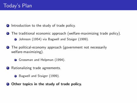
Today’s Plan









1

2

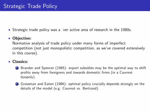
Strategic Trade Policy

• Strategic trade policy was a ver active area of research in the 1980s.

• Objective: Normative analysis of trade policy under many forms of imperfect competition (not just monopolistic competition, as we’ve covered extensively in this course).

Classics:•

Brander and Spencer (1985): export subsidies may be the optimal way to shift profits away from foreigners and towards domestic firms (in a Cournot duopoly).

Grossman and Eaton (1986): optimal policy crucially depends strongly on the details of the model (e.g. Cournot vs. Bertrand).

Strategic Trade Policy (Cont.)

• Recently, a few papers have revisited the implication of imperfect competition for trade agreements. In particular, does imperfect competition provide a new rationale for trade agreements?

• Ossa (2011) uses a monopolistic competition model as in Krugman (1980). Recall that this model features a ‘purely domestic’ineffi ciency if there is more than one industry, due to the home market effect. Hence Ossa (2011) says, “yes.”

• Bagwell and Staiger (2009) argue that this result obtains in Ossa (2011) because that paper restricts government trade policy to only include import tariffs. Hence they say, “no.”

• From an empirical standpoint:

• Can we figure out which assumptions about market structure fit best a given industry? If so, why would Grossman and Eaton (1986) be a problem?

• There have of course been huge advances in empirical IO (eg estimation in settings with strategic interactions) since 1986.

Why Do Governments Use Trade Policy Instruments?

• Most papers analyzing trade policy start from ad-hoc restriction on the set of instruments (e.g. tariffs, quotas, export subsidies, no production subsidies).

• Conditional on this ad-hoc restriction, paper then explains why trade policy may look the way it does and what its consequences may be.

• But why would governments use ineffi cient instruments in the first place?

• In developing countries, this may be the “best feasible” way to raise revenues (Gordon and Li, 2005).

• Ineffi cient methods may be used to reduce total redistribution (Dixit, Grossman and Helpman,1997).

• Ineffi cient redistribution may be used as a commitment device (Acemoglu and Robinson, 2001).

Understanding the WTO

• What are the implications of the self-enforcing nature of trade agreements?

• Bagwell and Staiger (1990), Maggi (1996).

• What is the rationale for trade agreements in the presence of NTBs?

• Bagwell and Staiger (2001) consider the case of product standards (and conclude that, once again, only the terms-of-trade externality matters).

• How can we rationalize simple rigid rules (e.g. an upper bound on tariffs) within the WTO?

• Amador and Bagwell (2010), Horn, Maggi, and Staiger (2010).

• Quantitatively, how large are the gains from the WTO?

MIT OpenCourseWare http://ocw.mit.edu

14.581 International Economics ISpring 2011

For information about citing these materials or our Terms of Use, visit: http://ocw.mit.edu/terms.

http://ocw.mit.edu/terms

http://ocw.mit.edu

mit phd international trade 25: trade...

Documents