14.581 international trade — — | lecture 10: … international trade | lecture 10:...

— —

14.581

Spring 2013

14.581 RV and HO Empirics (I) Spring 2013 1 / 55

14.581 International Trade— Lecture 10: Heckscher-Ohlin Empirics (I) —

14.581

Spring 2013

Plan of Today’s Lecture

1

2

Empirical work on Ricardo-Viner model: Introduction Factor price responses to goods price changes:

1

2

1

2

Stock market event study approach: Grossman and Levinsohn (1987) Political economy approaches: Magee (1980), Mayda and Rodrik (2005)

3 GNP function approach: 1 Kohli (1993)

4 ‘Geographic Incidence’ approaches: 1

2

Topalova (2009) Kovak (2009)

5 Areas for future research

Empirical work on Heckscher-Ohlin model (part I): 1

2

Introduction Tests concerning the ‘goods content’ of trade



1

2

Empirical work on Ricardo-Viner model: Introduction 1

2 Factor price responses to goods price changes: 1

2


3

4

GNP function approach: 1 Kohli (1993)

‘Geographic Incidence’ approaches: 1

2




2



Empirical Work on the Ricardo-Viner Model

Very little empirical work on the RV model. Why? RV model is best thought of as the short- to medium-run of the H-O model so you’d expect an integrated, dynamic empirical treatment of the two models. However, most H-O empirics is done using a cross-section, which is usually thought of as a set of countries in long-run equilibrium. Hence, there was never a pressing need to think about adjustment dynamics (ie the SF model).

There is probably also a sense that a serious treatment of these dynamics is too complicated for aggregate data (even if aggregate panel data were available).

The heightened availability of firm-level panel data opens up new possibilities.

We will look here at papers that have identified and tested aspects of RV model that are unique to RV model (at least relative to H-O).



1

2

Empirical work on Ricardo-Viner model: 1

2

Introduction Factor price responses to goods price changes:


1

2

3

4



2




2



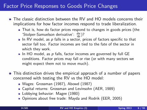
Factor Price Responses to Goods Price Changes

The classic distinction between the RV and HO models concerns their implications for how factor incomes respond to trade liberalization.

That is, how do factor prices respond to changes in goods prices (the dw‘Stolper-Samuelson derivative’: )?dp

In RV model, as p falls in a sector, prices of factors specific to that sector fall too. Factor incomes are tied to the fate of the sector in which they work. In HO model, as p falls, factor incomes are governed by full GE conditions. Factor prices may fall or rise (or with many sectors we might expect them not to move much).

This distinction drives the empirical approach of a number of papers concerned with testing the RV vs the HO model:

Wages: Grossman (1987), Abowd (1987) Capital returns: Grossman and Levinsohn (AER, 1989) Lobbying behavior: Magee (1980) Opinions about free trade: Mayda and Rodrik (EER, 2005)


Grossman and Levinsohn (1989)

Testing the effect of goods price changes on factor returns:

Using wages is attractive: there is (probably) something closer to a ‘spot market’ (at which we observe the going price) for labor than there is for machines.

Using capital returns is also attractive: Can (with some assumptions) use data from stock markets, which provides high quality and high-frequency data, as well as the usual opportunities for an ‘event study’ approach. (We are perhaps more likely to believe this is a setting where prices are set by forward-looking, rational agents facing severe arbitrage pressures.)

In an innovative paper, GL (1989) follow the latter approach.


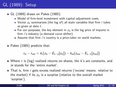
GL (1989): Setup

GL (1989) draws on Pakes (1985): Model of firm-level investment with capital adjustment costs. Vector zit summarizes (the log of) all state variables that firm i takes as given at date t. For our purposes, the key element in zit is the log price of imports in firm i ’s industry (a demand curve shifter). Assume that firm i ’s country is a price-taker on world markets.

Pakes (1985) predicts that:

rit − rmt = ki (zit − Et−1[zit ]) − km(zmt − Et−1[zmt ])

Where r is (log) realized returns on shares, the k’s are constants, and m stands for the ‘entire market’.

That is, firm i gets excess realized returns (‘excess’ means: relative to the market) if its zit is a surprise (relative to the overall market ‘surprise’).


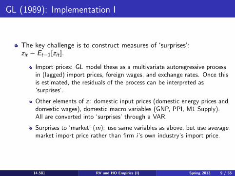
GL (1989): Implementation I

The key challenge is to construct measures of ‘surprises’: zit − Et−1[zit ].

Import prices: GL model these as a multivariate autoregressive process in (lagged) import prices, foreign wages, and exchange rates. Once this is estimated, the residuals of the process can be interpreted as ‘surprises’.

Other elements of z : domestic input prices (domestic energy prices and domestic wages), domestic macro variables (GNP, PPI, M1 Supply). All are converted into ‘surprises’ through a VAR.

Surprises to ‘market’ (m): use same variables as above, but use average market import price rather than firm i ’s own industry’s import price.


GL (1989): Implementation II

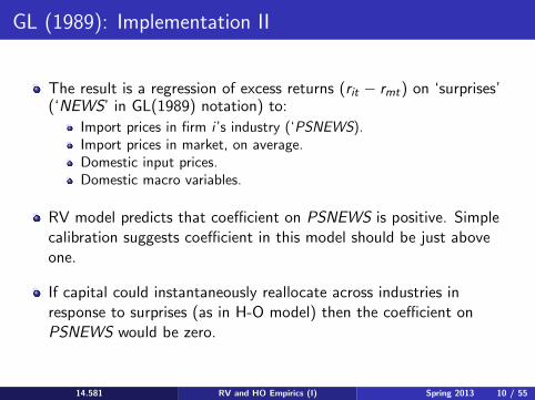
The result is a regression of excess returns (rit − rmt ) on ‘surprises’ (‘NEWS’ in GL(1989) notation) to:

Import prices in firm i ’s industry (‘PSNEWS). Import prices in market, on average. Domestic input prices. Domestic macro variables.

RV model predicts that coefficient on PSNEWS is positive. Simple calibration suggests coefficient in this model should be just above one.

If capital could instantaneously reallocate across industries in response to surprises (as in H-O model) then the coefficient on PSNEWS would be zero.


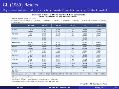
GL (1989) Results Regressions run one industry at a time; ‘market’ portfolio m is entire stock market


PSNEWS

WSNEWS

ERNEWS

AGGMNEWS

PENEWS

WNEWS

GNPNEWS

PPINEWS

MSNEWS

R2

No. of firms inSIC group

Estimation period 1974:2 to 1985:4

-0.870b

4.424b -4.828b

-0.776b

0.908b

2.922b

2.726

3.029b

0.083

1.217b

(0.449)

-0.648(0.834)

_

-0.044(0.275)

-0.164

(1.21)

(1.17)

0.345(1.07)

(1.23)

0.097

9

(0.356)

4.376b

2.825b

2.784b

0.476c

-0.209

0.724

0.192

0.310

1.585

2.565

0.156

5

1974:3 to 1986:3

2.675

3.080c

0.093

7

1976:3 to 1986:3

1.584c

0.827c

1.230

0.133

-0.112

-0.173

0.225

1.470

1.407

0.117

1.279

2.071

_

-0.410

(1.21)

(0.784)

(0.414)

(0.454)

(1.81)

(1.83)

(1.59)

(0.280)

(1.68)

(2.83)

(0.498)

(0.486)

(1.89)

(1.83)

(1.86)

(1.25)

(1.63)

-0.357

-1.115

_

0.351

-0.547

1.166

4.628b

2 16 16

4.167c

1.152

-2.214

_

0.103

-0.542

0.773

1.494

0.172

(0.819)

(1.59)

(0.499)

(0.561)

(2.18)

(2.03)

(2.18)

(1.99)

1975:2 to 1986:3 1974:2 to 1986:3 1975:1 to 1984:2

(0.476)

(0.854)

(0.442)

(0.219)

(0.255)

(1.10)

(0.902)

(0.853)

(0.978)

(0.343)

(1.43)

(0.386)

(0.487)

(1.78)

(1.56)

(1.62)

(1.62)

Determinants of Excess Return: qit - Γ1 PSNEWSnt + Γ2WSNEWSt + Γ3 ERNEWSt + Γ4 AGGMNEWSt + Γ5 PENEWSt + Γ6 WNEWSt + Γ7 GNPNEWSt + Γ8 PPINEWSt+ Γ9 MSNEWSt + νit

Definition of Excess Return: qit = rit - rmt

SIC 262 SIC 242 SIC 301 SIC 345 SIC 32 SIC 331

aStandard errors in parentheses.bSignificantly different from zero at the 5 percent level, two-tailed test.cSignificantly different from zero at the 10 percent level, two-tailed test.

Estimation pf Random-Effects Model with Time Components(Base Case Results for Risk Netural Version)a

Image by MIT OpenCourseWare.

Magee (1980): “Simple Tests of the S-S Theorem”

Magee (1980) collects data from testimony given in a Congressional committee on the Trade Reform Act of 1973.

29 Trade associations (“representing management”) and 23 labor unions expressed whether they were for either freer trade or greater protection. These groups belong to industries.

Striking findings, in favor of RV model (and against simple version of the S-S Theorem/HO model):

K and L tend to agree on trade policy within an industry (in 19 out of 21 industries). Each factor is not consistent across industries. (Consistency is rejected for K, but not for L). The position taken by a factor (in an industry) is correlated with the industry’s trade balance.

1

2

3

Relatedly: As we shall see later in the course, lobbying models (most prominently: Grossman and Helpman (AER, 1994)) typically make the RV assumption for tractability.

Goldberg and Maggi (AER, 1999) find empirical support for this in the US tariff structure.


Mayda and Rodrik (EER, 2005)

Mayda and Rodrik (2005) exploit internationally-comparable surveys (such as the World Values Survey) to look at how national attitudes to free trade differ across, and within, countries.

Findings support both HO and RV models: HO: People in a country are more likely to oppose trade reform if they are relatively skilled and their country is relatively skill-endowed. (Recall S-S: trade reform favors scarce factors.)

RV: People in import-competing industries are more likely to oppose trade reform (than those in non-traded industries).



1

2


2


1

2


3

4



2




2



Kohli (JIE, 1993): Introduction

Kohli (1993) pursues a different distinction between RV and HO. Basic idea:

In a standard neoclassical economy, profit maximization leads to maximization of the total value of ouptut (or ‘GNP’).

Further, the revenue (or ‘GNP’) function summarizes all information about the supply-side of the economy.

The solution to revenue maximization problem should depend, in some way, on whether the maximization is ‘constrained’ (some factor cannot move across sectors, ie the RV model) or ‘unconstrained’ (all factors can move, ie the HO model).

Kohli (1993) searches for a way to isolate how constrained and unconstrained GNP functions look in general, and then tests for this.


Kohli (1993): Details I

Kohli (1993) works with the (net) restricted GNP/revenue function (Diewert, 1974):

RR(p1, p2, w , K ) ≡ max {p1y1 + p2y2 − wL : (y1, y2, L, K ) ∈ T }y1,y2,L

Where p is the goods price (in sector 1 or 2), y is output, L and K are labor and capital endowments, w is the wage, and T is the feasible technology set. Here ‘restricted’ means that the allocation of K is fixed across sectors. Only L can be allocated to maximize (net) revenue/GNP.

This is homogeneous (of degree 1) in K : RR(p1, p2, w , K ) = r(p1, p2, w)K .


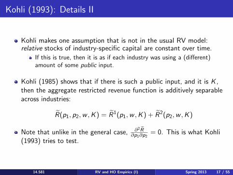
Kohli (1993): Details II

Kohli makes one assumption that is not in the usual RV model: relative stocks of industry-specific capital are constant over time.

If this is true, then it is as if each industry was using a (different) amount of some public input.

Kohli (1985) shows that if there is such a public input, and it is K , then the aggregate restricted revenue function is additively separable across industries:

RR(p1, p2, w , K ) = RR1(p1, w , K ) + RR2(p2, w , K )

∂2 RNote that unlike in the general case, R = 0. This is what Kohli ∂p1∂p2

(1993) tries to test.


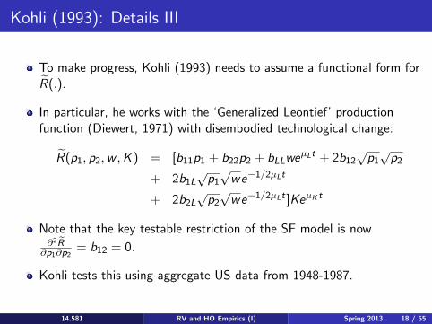
Kohli (1993): Details III

To make progress, Kohli (1993) needs to assume a functional form for RR(.). In particular, he works with the ‘Generalized Leontief’ production function (Diewert, 1971) with disembodied technological change:

RR(p1, p2, w , K ) = [b11p1 + b22p2 + bLLweµLt + 2b12

√ p1 √ p2

√ √ −1/2µLt+ 2b1L p1 we

+ 2b2L √ p2 √ we −1/2µLt ]KeµK t

Note that the key testable restriction of the SF model is now ∂2RR = b12 = 0. ∂p1∂p2

Kohli tests this using aggregate US data from 1948-1987.


Kohli (1993) Results I Two ‘goods’ (1 and 2) are Consumption and Investment. Also presented are joint cost function estimates (dual to the revenue function).


aCC

aKK

aIC

aIK

aCK

µL

µK

LL

aII 932.15

8,5411.8

6,774.0

311.31

-766.12

-6,949.5

0.01052

0.00203

-494.59

0.94849Rp2

bCC

bLL

bIC

bIL

bCL

µL

µK

LL

bII

Rp2

(16.30)

(20.09)

(15.29)

(2.86)

(-7.18)

(-16.67)

(12.01)

(3.25)

8,919.6

6,557.4

_

-527.22

-6,994.4

0.00967

0.00335

1,002.8

-498.19

0.94531

(21.76)

(15.31)

(-8.83)

(-16.66)

(10.06)

(18.71)

(6.77)

4,734.8

1,982.9

-103.59

-1,170.2

-2,485.2

0.01504

0.00196

2,000.4

-505.20

0.93852

(24.37)

(4.71)

(-0.66)

(-3.85)

(-10.12)

(18.90)

(6.59)

(4.04)

4,730.6

2,144.7

_

-1,238.4

-2,581.0

0.01500

0.00216

1,964.5

-505.42

0.93831

(6.54)

(24.56)

(6.25)

(-4.25)

(-13.31)

(18.19)

(5.42)

Notes:JP: Joint productionANJIPQ: Almost non-jointness in input price and quantities

Parameter Estimates (t-Value in Parentheses)

JP ANJIPQ JP ANJIPQ

Restricted joint cost function Revenue function


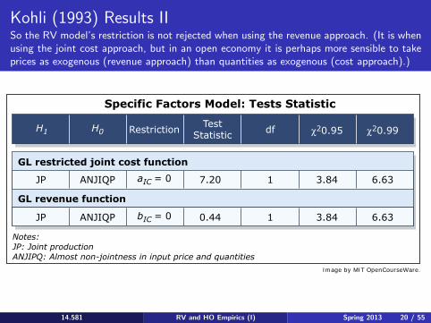
Kohli (1993) Results II So the RV model’s restriction is not rejected when using the revenue approach. (It is when using the joint cost approach, but in an open economy it is perhaps more sensible to take prices as exogenous (revenue approach) than quantities as exogenous (cost approach).)


GL restricted joint cost function

GL revenue function

JP ANJIQP

RestrictionTest

Statistic

JP ANJIQP

7.20

0.44

1

1

3.84

3.84

6.63

6.63

aIC = 0

bIC = 0

H1 H0 df χ20.95 χ20.99

Notes:JP: Joint productionANJIPQ: Almost non-jointness in input price and quantities

Specific Factors Model: Tests Statistic



1

2


2


1

2


3

4


‘Geographic Incidence’ approaches: Topalova (2009) Kovak (2009)

1

2



2



‘Regional Incidence’ of Trade Shocks

Suppose a change in trade policy affects p (one nation-wide goods price vector). How does this affect welfare (ie, real income, here) in different regions of a country?

This has been an important topic in the field of ‘Trade and Development’.

This is the question that Topalova (AEJ Applied, 2009) and Kovak (2009) propose, with respect to India and Brazil, respectively.

Porto (JIE, 2005), among others, also looks at this question.

The RV model (often implicitly) has been an influential theoretical approach within which to attack this empirical question.

Topalova (2009): labor is intersectorally immobile and geographically immobile Kovak (2009): labor is intersectorally immobile but geographically mobile


Topalova (2009)

In an innovative paper, Topalova (2009) estimates the following regression on Indian districts:

ydt = αd + βt + γTariffdt + εdt

Here, y is the poverty rate, and Tariffdt is calculated as the district employment-weighted average of national industry-wise tariffs. India is attractive here for many reasons:

India went through an important and controversial trade liberalization in 1991 (and later in the 1990s). There are very good, long-running surveys of poverty, for which the micro data is available from (roughly) 1983 onwards. There are 400-600 districts, depending on the time period.

Topalova (2009) uses a (now standard) IV for tariffs: In trade liberalization episodes, higher tariffs have ‘further to fall’. So a plausible instrument for tariff changes is pre-liberalization tariff levels.


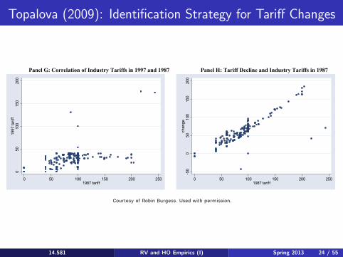
Topalova (2009): Identification Strategy for Tariff Changes

Figure 1. Evolution of Tariffs in India

Panel G: Correlation of Industry Tariffs in 1997 and 1987 Panel H: Tariff Decline and Industry Tariffs in 1987

Panel A: Average Nominal Tariffs

0

20

40

60

80

100

120

1987 1988 1989 1990 1991 1992 1993 1994 1995 1996 1997 1998 1999 2000 2001

Panel B: Standard Deviation of Nominal Tariffs

0

10

20

30

40

50

60

1987 1988 1989 1990 1991 1992 1993 1994 1995 1996 1997 1998 1999 2000 2001

Panel C: Tariffs by Broad Industrial Category

0

20

40

60

80

100

120

1987

1989

1991

1993

1995

1997

1999

2001

Cereals andOilseedsAgriculture

Mining & Mfg-K

Mining & Mfg-C

Panel D: Tariffs by Industrial Use Based Category

0

20

40

60

80

100

120

1987

1989

1991

1993

1995

1997

1999

2001

Basic

Capital

ConsumerDurablesConsumer NonDurablesIntermediate

Panel E: Share of Free HS Lines by Broad Industrial Category

0

0.2

0.4

0.6

0.8

1

1.2

1989 1996 1998 2001

Cereals & OilseedsAgricultureMining & Mfg-KMining & Mfg-C

Panel F: Share of Free HS Lines by Industrial Use Based Category

0

0.2

0.4

0.6

0.8

1

1.2

1989 1996 1998 2001

Basic

Capital

Consumer Durables

Consumer NonDurablesIntermediate

050

100

150

200

1997

tarif

f

0 50 100 150 200 2501987 tariff-5

00

5010

015

020

0ch

ange

0 50 100 150 200 2501987 tariff


Courtesy of Robin Burgess. Used with permission.

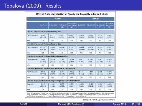
Topalova (2009): Results


Panel A. Dependent Variable: Poverty Rate

Panel B. Dependent Variable: Poverty Gap

Panel C. Dependent Variable: StdLog Consumption

Panel D. Dependent Variable: Log Deviation of Consumption

Panel E. Dependent Variable: Log Average Per Capita Expenditure

Tariff measure

Obs

Tariff measure

Obs

Tariff measure

Obs

Obs

Tariff measure

Obs

Logmean

-0.287** -0.297*** -0.834*** -0.687*** -0.215 -0.065 -0.156 -0.403(0.118) (0.084) (0.250) (0.225) (0.190) (0.156) (0.353) (0.257)

725 725 725 725 703 703 703 703

-0.129*** -0.114*** -0.319*** -0.206*** -0.084 -0.032 -0.076 -0.131

(0.038) (0.021) (0.073) (0.075) (0.052) (0.046) (0.101) (0.087)

725 725 725 725 703 703 703 703

-0.086 -0.094 -0.265 -0.161 0.092 0.108 0.257 0.213

(0.154) (0.082) (0.228) (0.183) (0.094) (0.115) (0.295) (0.250)

725 725 725 725 703 703 703 703

725 725 725 725 703 703 703 703

725 725 725 725 703 703 703 703

(0.066) (0.042) (0.115) (0.071) (0.062) (0.066) (0.174) (0.144)

(0.314) (0.183) (0.522) (0.433) (0.150) (0.212) (0.521) (0.468)

-0.016 -0.020 -0.057 -0.020 0.034 0.090 0.215 0.172

-0.015 0.132 0.370 0.552 -0.063 -0.126 -0.301 0.048

(7)(4)(3) (8)Tariff (1) TrTariff(2) IV-TrTariff

IV-TrTariffInitTrTariff Tariff (5) TrTariff (6) IV-TrTariff

IV-TrTariffInitTrTariff

Rural Urban

Note: All regressions include year and district dummies. Standard errors (in parentheses) are corrected for clustering at the state yearlevel. Regressions are weighted by the square root of the number of people in a district. Significance at the 10 percent level ofconfidence is represented by a *, at the 5 percent level by **, and at the 1 percent level by ***.

Effect of Trade Liberalization on Poverty and Inequality in Indian Districts


Kovak (2009)

Kovak (2009) performs a similar exercise to Topalova (2009), but with some attractive extensions:

The estimating equation emerges directly from a RV model.

The estimating equation is similar to Topalova (2009), but with a slight alteration to the way that Tariffdt is calculated (he uses different weights and different treatment of the non-traded sector).

Unlike Topalova (2009), Kovak (2009) finds economically and statistically significant migration responses: people appear to move around the country in response to (national) tariff changes, to get closer to favored industry-specific factors like capital/land.



1

2


2


1

2


3

4



2



Empirical work on Heckscher-Ohlin model (part I): Introduction Tests concerning the ‘goods content’ of trade

1

2


Areas for Future Research

Tracing the short-, medium- and long-run adjustment to trade liberalizations or other ‘natural experiments’.

Can RV and HO models be unified in the data as the same model with different time horizons?

Ideally one could use firm-level panel data (which we will see lots of later in the course).

Trefler (2004 AER) does this well for Canada’s liberalization (CUSFTA), as we will see later. But focus there was on productivity changes, rather than factor adjustment/mobility.

Muendler and Menezes-Filho (2007) exploit rich data on Brazilian matched employer-employee records to track workers around a trade liberalization episode.


Areas for Future Research

Adjustment to trade liberalization with proper micro-founded adjustment costs, estimated rigorously:

Capital market adjustment frictions: Caballero-Engel (various), Bloom (Ecta, 2008); could potentially exploit US Census Data Center in Boston)

Labor market adjustment frictions: McLaren and Choudhuri (AER, 2010) on idiosyncratic location-specific utilities; Tybout et al (2009) on search frictions; Dix-Carneiro (2010 JMP).

Further applications of the GL (1989) event-study approach to Trade questions?



1

2


1

2

1

2


3

4



2



Empirical work on Heckscher-Ohlin model (part I): Introduction 1

2 Tests concerning the ‘goods content’ of trade


Introduction to HO Empirics

The H-O model is probably the most influential model in all of Trade. So how do we assess how useful a description of the real world it is?

One immediate obstacle is that the theory’s predictions aren’t that precise.

The 2 × 2 model makes precise predictions, but (without putting more structure on the problem) not much of this generalizes to higher dimensional settings (Ethier (1984, Handbook chapter)).

As we have seen, this is a familiar problem from wider Comparative Advantage settings (including the Ricardian model)


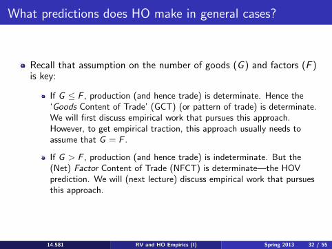
What predictions does HO make in general cases?

Recall that assumption on the number of goods (G ) and factors (F ) is key:

If G ≤ F , production (and hence trade) is determinate. Hence the ‘Goods Content of Trade’ (GCT) (or pattern of trade) is determinate. We will first discuss empirical work that pursues this approach. However, to get empirical traction, this approach usually needs to assume that G = F .

If G > F , production (and hence trade) is indeterminate. But the (Net) Factor Content of Trade (NFCT) is determinate—the HOV prediction. We will (next lecture) discuss empirical work that pursues this approach.


Aside: How many goods and factors are there?

Clearly, as we map from this model to the real world, the G ≥≤ F question really hangs on our level of aggregation (every worker is different in some dimension!)

And of course ‘aggregation’ is really just at what level we assume goods/factors are perfect substitutes so that they can be trivially aggregated.

A different approach is pursued by Bernstein and Weinstein (JIE, 2002), who examine whether G ≥ F seems more plausible by testing the indeterminacy of production (conditional on endowments) in a G > F world.



1

2



1

2

1

2

3

4



2




2



Introduction to ‘Goods Content’ of Trade Tests

Now we focus on the case of G ≤ F , and ask whether the H-O model’s predictions for trade (or output) of goods find support in the data.

Also called ‘Rybczinski regressions’.

Brief chronology: Baldwin (1971): not quite the right test Leamer (1984, book): first pure test on trade flows Harrigan (JIE, 1995): same as Leamer (1984) but on output Harrigan (AER, 1997): adding technology differences Schott (AER, 2001): multiple cones of specialization Romalis (AER, 2004) (and Morrow (2009)): actually G > F , but production indeterminacy broken by trade costs (and hence lack of FPE).


H-O Theory with G ≤ F , Part I

Recall the revenue function (for country c): c c c cY c = r c (p , V c ) ≡ maxyc {p .y : y ∈ T (V c )}.

Here Y is total GDP, y is the vector of outputs (in each sector), p is the vector of prices, and T is the technology set.

c cThen we have (with G ≤ F ): y = Vprc (p , V c ), which is

homogeneous of degree one in V c by CRTS. Recall that with G > F , this becomes a correspondence (ie production is indeterminate), not an equality.

c c cAnd hence: y = VpV rc (p , V c ).V c ≡ Rc (p , V c ).V c .

cRc (p , V c ) is often called the ‘Rybczinski matrix’.


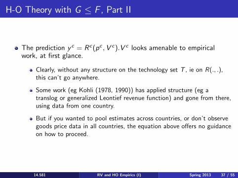
H-O Theory with G ≤ F , Part II

c cThe prediction y = Rc (p , V c ).V c looks amenable to empirical work, at first glance.

Clearly, without any structure on the technology set T , ie on R(., .), this can’t go anywhere.

Some work (eg Kohli (1978, 1990)) has applied structure (eg a translog or generalized Leontief revenue function) and gone from there, using data from one country.

But if you wanted to pool estimates across countries, or don’t observe goods price data in all countries, the equation above offers no guidance on how to proceed.


H-O Theory with G ≤ F , Part III

The more influential ‘Trade’ approach has been to further assume that G = F (the ‘even case’). Then:

The factor market clearing conditions imply immediately that c c c(assuming Ac (w , V c ) is invertible): y = [Ac (w , V c )]−1V c

c cSo Rc (p , V c ) = [Ac (w , V c )]−1 .

And if we confine attention to an FPE equilibrium (identical technologies (ie Ac (., .) = A(., .)), no trade costs, no factor intensity reversals, and endowments inside the FPE set) then ‘factor price insensitivity’ holds: A(w , V c ) = A(w). (ie techniques used are locally independent of V c .)

cSimilarly: Rc (p , V c ) = R(p) —that is, all countries have the same Rybczinski (or A) matrix.


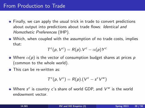
From Production to Trade

Finally, we can apply the usual trick in trade to convert predictions about output into predictions about trade flows: Identical and Homothetic Preferences (IHP).

Which, when coupled with the assumption of no trade costs, implies that:

T c (p, V c ) = R(p).V c − α(p)Y c

Where α(p) is the vector of consumption budget shares at prices p (common to the whole world).

This can be re-written as:

T c (p, V c ) = R(p).(V c − s c V w )

cWhere s is country c ’s share of world GDP, and V w is the world endowment vector.


Baldwin (1971) I

Theory: T c (p, V c ) = R(p).(V c − sc V w )

Baldwin (1971) was the first to explore the implications of this equation empirically.

He could have either: 1 Taken data on T c (p, V c ), R(p) = [A(w)]−1, and (V c − sc V w ), to

check this prediction exactly. As we’ll discuss next lecture, one can obtain data on A(w) from input-output accounts.

2

3

Or, regressed T c (p, V c ) on R(p) = [A(w)]−1 to check whether the estimated coefficients take the same signs/magnitudes as (V c − sc V w )

Or, regressed T c (p, V c ) on (V c − sc V w ) to check whether the estimated coefficients take the same signs/magnitudes as R(p) = [A(w)]−1

Baldwin (1971) did 2. Leamer (1984) did a version of 3.


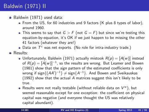
Baldwin (1971) II

Baldwin (1971) used data: From the US, for 60 industries and 9 factors (K plus 8 types of labor), around 1960. This seems to say that G > F (not G = F ) but since we’re testing this equation-by-equation, it’s OK if we just happen to be missing the other 41 factors (whatever they are!) Data on T c was net exports. (No role for intra-industry trade.)

Results: Unfortunately, Baldwin (1971) actually mistook R(p) = [A(w)] instead of R(p) = [A(w)]−1, so the results are wrong. But Leamer and Bowen (1981) show that the sign pattern of the estimated coefficients is only wrong if sign{(AA')−1} And Bowen and Sveikauskas = sign{A−1}. (1992) show that the actual A matrices suggest this isn’t likely to be true. Results were not really testable (without reliable data on V w ), but seemed reasonable except for one exception: the coefficient on physical capital was negative (and everyone thought the US was relatively capital abundant).


Leamer (1984 book): Set-up

Leamer instead treats (V c − sc V w ) as data and regresses T c (p, V c ) on (V c − sc V w ).

Really, this amounts to estimating the regression equation FT c = βik (V c − sc V w ) + εc across countries c , one commodity i k=1 k k i i at a time.

The coefficients βik are often called ‘Rybczinski effects’.


Leamer (1984): Data

Leamer (1984) did a huge amount of pioneering work in compiling data on trade flows and factor endowments.

60 countries, two different years (1958 and 1975)

Goods classifications: Leamer organizes the data into 10 goods, deliberately aggregating over some finer-level data in order to find ‘industries’ in which exports appear to flow the same way (within industries), and capital-worker and professional worker-all worker ratios are similar within industries. (So industries look roughly similar along taste and technology dimensions.)

Factors: K, 3 types of L, 4 types of land (distinguished by climate), and 3 types of natural resources.

11 Goods (10 plus non-traded goods) and 11 Factors (‘even’ !)


Leamer (1984): Results and Interpretation I

Leamer (1984) stresses that point estimates shouldn’t be taken too seriously. But that coefficient signs should be, especially when they’re precisely estimated.

But how do we interpret the signs here? The signs should all be equal to the signs on [A(w)]−1 . But Leamer (1984) doesn’t pursue this (I don’t know why not).

HO theory says nothing (beyond 2 × 2) about the signs we should expect on R(p) = [A(w)]−1 .

With one exception: Jones and Sheinkman (1977) show that for each good i , one coefficient βik should be positive and one should be negative. (“Friends and Enemies”). Leamer (1984) indeed finds this to be true (though that is of course a weak test). Harrigan (2003, Handbook survey) argues that this is a nice example of evidence for GE forces in the data.


Leamer (1984): Results and Interpretation II

Leamer (1984) has a great discussion of how we could interpret some of the precisely-estimated coefficients:

Eg: in manufacturing, the coefficient on capital is positive (which perhaps seems sensible).

But in manufacturing, the coefficient on land is negative. (Note that this is the sort of surprising result you could never find in an industry-by-industry production function estimation approach.) Why? Perhaps because a country with lots of land specializes in agriculture, and this draws other resources out of manufacturing. However, this could of course just be sampling variation (ie some coefficient(s) may be negative simply by ‘luck’).

These are plausible interpretations, but there is nothing in general HO theory that says these need to be true.


Harrigan (JIE, 1995) I

Harrigan (1995 and 2003) argues that the real intellectual content of HO theory concerns production, not consumption, and hence not trade at all!

The addition of the IHP assumption to convert a prediction about production into a prediction about trade, he argues, is at best a distraction, and at worse very misleading (since IHP isn’t likely to be true.)

Of course, that isn’t to imply that enriching the IHP assumption isn’t worth doing if the goal is to explain trade flows.

A key reason for Leamer (1984) to use trade data rather than output data was not just his interest in trade—he lacked comparable output data across countries. (Trade data has been good and plentiful around the world for centuries longer than any other type of data.) By the early 1990s, however, the OECD had started to make comparable output data available to researchers, so Harrigan uses this.


Harrigan (JIE, 1995) II

So Harrigan (1995) pursues the Leamer (1984) approach using output data instead of export data.

The results are similar to Leamer’s.

But he highlights that an overall disappointment is that the R2 is very low.

In other words, the production-side assumptions made in conventional HO theory are incapable of capturing much of the variation in output across countries and industries (and years).


Harrigan (AER, 1997)

Harrigan (1997) starts from the premise that (what is probably) the most egregious assumption in conventional HO theory is that of identical technologies across countries.

But how to build non-identical technologies into the above framework?

That framework rested on the notion that since countries have identical technologies, and face identical goods prices due to free trade, and FPI and FPE hold, R(.) is identical across countries. And we can therefore estimate R(.) using variation in V c across countries.

Harrigan’s solution was to add more structure to the set-up. He assumed a particular (but flexible—‘superlative’, in the language of Diewert (1976)) functional form for the revenue function.


Harrigan (1997): Set-up I

Harrigan assumes a translog revenue function.

To this he adds Hicks-neutral productivity difference in each country and sector: θi

c .

With the additional restriction that all countries face the same prices p and that the translog is CRTS (and fixed over time), he derives the following estimation equation:

F θc GF F V c

c kt s = αit + aki ln + rij lnjt

it θc V c 1t jtk=2 j=2

cHere, sit is the share of output of sector i in country c ’s GDP in year t, αit is a sector-year fixed effect, and the parameters aki and rij are the translog parameters.

It turns out that this revenue function also has implications for factor shares which could be tested in principle.


Harrigan (1997): Set-up II

A complication is the presence of non-traded goods:

That is, there are some elements of the price vector which are not equalized across countries and that will therefore not be absorbed into the αit fixed effect.

In particular, there will now be terms involving non-traded goods prices and non-traded sectors’ productivities.

Harrigan (1997) argues that these terms might be soaked up in a fixed effect at the country-good level, and if not, they might be orthogonal to the terms included above.


Harrigan (1997): Implementation

Harrigan estimates the above equation using a panel of countries and industries.

He estimates the equation one good at a time (with country and year fixed effects), but in a SUR sense (since the dependent variable is a share so all dependent variables sum to one).

Note that the data requirements go beyond Harrigan (1995): Harrigan (1997) requires data on TFP by industry and country.

He also instruments TFP (in fear of classical measurement error), using the average of other countries’ TFPs as the instrument (sector by sector).


Harrigan (1997): Results


TFP Food

TFP Apparel

TFP Paper

TFP Chemicals

TFP Glass

TFP Metals

TFP Machinery

Prod. durables

Nonres. const.

High-ed. workers

Medium-ed workers

Low-ed. workers

Arable land

-0.457

0.672

0.144

-0.067

-0.327

0.381

0.005

1.305

-0.195

-0.170

0.682

-0.020

-1.602

(-2.01)

(4.74)

(1.09)

(-0.48)

(-3.21)

(3.55)

(0.02)

(6.90)

(-0.68)

(-1.34)

(3.47)

(-0.14)

(-5.27)

0.672

0.371

0.360

-0.485

-0.057

0.157

0.597

0.940

-0.353

-0.663

0.688

0.102

-0.714

(4.74)

(2.40)

(3.14)

(-4.25)

(-0.65)

(-1.92)

(3.39)

(6.57)

(-1.68)

(-7.16)

(4.88)

(0.99)

(-3.09)

0.144

0.360

0.184

-0.104

0.012

-0.003

0.387

-0.016

0.157

-0.219

-0.035

-0.148

-0.261

(1.09)

(3.14)

(1.06)

(-0.93)

(0.13)

(-0.04)

(2.34)

(-0.14)

(0.90)

(-2.98)

(-0.31)

(-1.78)

(1.43)

-0.067

-0.485

-0.104

2.025

-0.060

-0.029

-1.198

1.186

-1.530

-0.002

-0.889

-0.397

-1.631

(-0.48)

(-4.25)

(-0.93)

(11.9)

(-0.72)

(-0.29)

(-5.32)

(5.78)

(-5.26)

(-0.02)

(-4.44)

(-2.68)

(5.10)

-0.327

-0.057

0.012

-0.060

0.369

-0.107

-0.174

0.358

-0.244

-0.190

0.378

-0.103

-0.200

(-3.21)

(-0.65)

(0.13)

(-0.72)

(3.96)

(-1.82)

(-1.26)

(3.89)

(-1.70)

(-3.18)

(4.20)

(-1.53)

(-1.32)

0.381

-0.157

-0.003

-0.029

-0.107

0.618

-0.583

0.193

-0.066

-0.503

-0.210

-0.224

-0.809

(3.55)

(-1.92)

(-0.04)

(-0.29)

(-1.82)

(4.88)

(-3.00)

(0.96)

(-0.24)

(-3.93)

(-1.10)

(-1.55)

(2.64)

0.005

0.597

0.387

-1.198

-0.174

-0.583

3.583

0.193

-1.754

-2.114

1.013

1.820

0.123

(0.02)

(3.39)

(2.34)

(-5.32)

(-1.26)

(-3.00)

(6.06)

(1.91)

(-2.44)

(-6.60)

(2.11)

(5.22)

(0.14)

Food Apparel Paper Glass Metals MachineryChemicals

Estimates of the GDP Share Equations, Equation (5)

Notes: Estimation results are listed columns, with t-statistics in parentheses. The dependent variable is thepercentage share of the industry in GDP. All explanatory variables are in logarithms, and are listed as row.Country and year fixed effects are not shown. There are 203 observations in regression. For further details on


Harrigan (1997): Interpretation

The overall fit (R2), including fixed effects, is quite high: 0.95ish.

Leaves overall message that in fitting a world-wide revenue function, technology differences are important. As we will see next lecture, this echoes a persistent theme in the NFCT literature, post-Trefler (1993).

As theory would predict, the own-TFP effects (the bold diagonals) are almost always positive and statistically significant.

As theory would predict, some cross-TFP, and cross-endowment coefficients are negative, but the location of these negative coefficients isn’t very stable across specifications (see other tables).


Post-Harrigan (1997) I

Harrigan has room for non-FPE, but not for non-‘conditional FPE’ (in the language of Trefler (1993, JPE)).

c aPut another way, Ki should be a constant for any two factors (eg K caLi and L), within any good i and country c .

However, as will see next lecture, Davis and Weinstein (2001, AER) aKifind that in a regression like c

= βi + β Kc , the coefficient β is usually ca Lc

Li

large and statistically significant. (See also Dollar, Wolff and Baumol (1988, AER).)

That is, for some reason, even the relative techniques that countries use are affected by local relative endowments.

This stands in contrast to a HO model with Hicks-neutral TFP differences across countries and sectors.


Post-Harrigan (1997) II

Ways to rationalize this: 1 Country-industry technology differences are not Hicks-neutral. This is

probably true, but hasn’t generated much work (in ‘goods content’ of trade tests).

2 Trade costs prevent any sort of FPE (ie different countries face different pc ’s). This is also surely true (as we’ll see in a later lecture, trade costs appear to be very high). Romalis (2004) introduces trade costs into a special sort of (essentially 2-country) HO model to make progress here. Morrow (2009) extends this to include technology differences.

3 Countries are not all in the same cone of diversification (ie inside the ‘conditional FPE set’). Note that same cone of diversification means that all countries are incompletely specialized (ie all produce some of all goods), which sounds counterfactual. Schott (AER, 2003) builds on Leamer (JPE, 1987) and looks at whether Rybczinski regressions fit better if we allow countries to be in different cones.


MIT OpenCourseWarehttp://ocw.mit.edu

14.581 International Economics ISpring 2013

For information about citing these materials or our Terms of Use, visit: http://ocw.mit.edu/terms.

http://ocw.mit.edu

http://ocw.mit.edu/terms.

14.581 international trade — — | lecture 10: … international trade | lecture 10:...

Documents