14.581 International Trade Class notes on 3/19/20131

1 Introduction

• Hallak and Levinsohn (2005): “Countries don’t trade. Firms trade.”

• Since around 1990, trade economists have increasingly used data from individual firms in order to better understand:

– Why countries trade.

– The mechanisms of adjustment to trade liberalization: mark-ups, entry, exit, productivity changes, factor price changes.

– How important trade liberalization is for economic welfare.

– Who are the winners and losers of trade liberalization (across firms)?

• This has been an extremely influential development for the field. These are all new and interesting questions that a firm-level approach has enabled access to.

2 Stylized Facts about Trade at the Firm-Level

• Exporting is extremely rare.

• Exporters are different:

– They are larger.

– They are more productive.

– They use factors differently.

– They pay higher wages.

• We will go through some of these findings first.

2.1 Exporting is Rare

• Two papers provide a clear characterization of just how rare exporting activity is among firms:

• Bernard, Jensen, Redding and Schott (JEP, 2007) on US manufacturing.

1The notes are based on lecture slides with inclusion of important insights emphasized during the class.

1

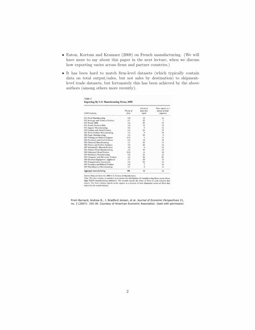
• Eaton, Kortum and Kramarz (2008) on French manufacturing. (We will have more to say about this paper in the next lecture, when we discuss how exporting varies across firms and partner countries.)

• It has been hard to match firm-level datasets (which typically contain data on total output/sales, but not sales by destination) to shipment-level trade datasets, but fortunately this has been achieved by the above authors (among others more recently).

2

From Bernard, Andrew B., J. Bradford Jensen, et al. Journal of Economic Perspectives 21,no. 3 (2007): 105-30. Courtesy of American Economic Association. Used with permission.

FRA

BEL NET

GERITAUNK

IRE DENGREPOR

SPA

NORSWE

FIN

SWI

AUT

YUGTUR USR

GEE CZEHUN

ROMBUL

ALB

MOR ALGTUN

LIY

EGY

SUD

MAU MAL BUKNIG

CHA

SEN

SIE LIB

COT

GHA

TOGBEN NIA

CAM

CEN ZAI

RWABUR ANG

ETH

SOM

KEN

UGA

TANMOZ

MAD MAS

ZAM ZIM

MAW

SOU

USA CAN

MEX

GUAHONELSNIC COS

PAN CUBDOM

JAM TRI

COL VEN

ECU PER

BRACHI

BOL

PAR URU

ARGSYR IRQ IRN

ISR

JOR

SAU KUW

OMA

AFG

PAK IND

BAN SRI

NEP

THA

VIE

INOMAY

SIN

PHI CHN

KOR

JAP

TAI

HOK AUL

PAP

NZE

10

100

1000

10000

100000

# fir

ms

sellin

g in

mar

ket

.1 1 10 100 1000 10000 market size ($ billions)

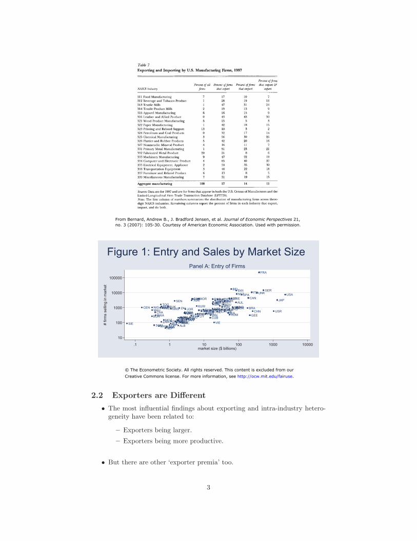
Panel A: Entry of Firms

Figure 1: Entry and Sales by Market Size

2.2 Exporters are Different

• The most influential findings about exporting and intra-industry hetero­geneity have been related to:

– Exporters being larger.

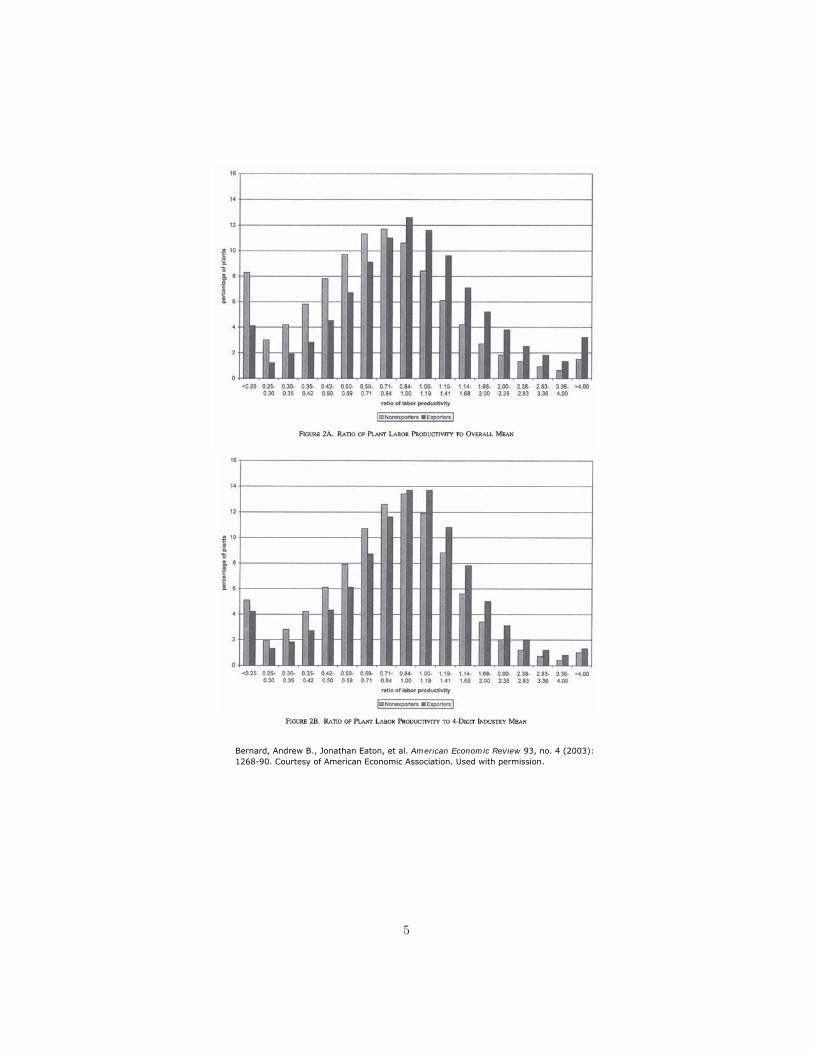
– Exporters being more productive.

• But there are other ‘exporter premia’ too.

3

© The Econometric Society. All rights reserved. This content is excluded from ourCreative Commons license. For more information, see http://ocw.mit.edu/fairuse.

From Bernard, Andrew B., J. Bradford Jensen, et al. Journal of Economic Perspectives 21,no. 3 (2007): 105-30. Courtesy of American Economic Association. Used with permission.

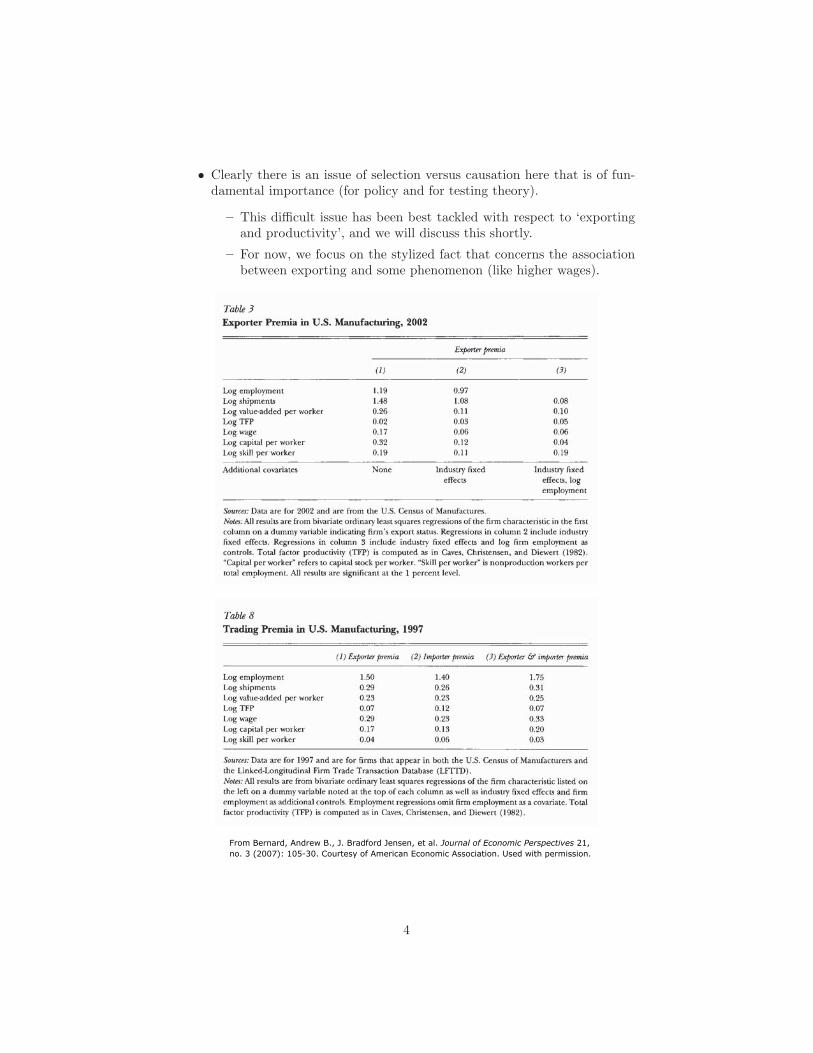
• Clearly there is an issue of selection versus causation here that is of fun­damental importance (for policy and for testing theory).

– This difficult issue has been best tackled with respect to ‘exporting and productivity’, and we will discuss this shortly.

– For now, we focus on the stylized fact that concerns the association between exporting and some phenomenon (like higher wages).

4

From Bernard, Andrew B., J. Bradford Jensen, et al. Journal of Economic Perspectives 21,no. 3 (2007): 105-30. Courtesy of American Economic Association. Used with permission.

5

Bernard, Andrew B., Jonathan Eaton, et al. American Economic Review 93, no. 4 (2003):1268-90. Courtesy of American Economic Association. Used with permission.

aver

age

prod

uctiv

ity

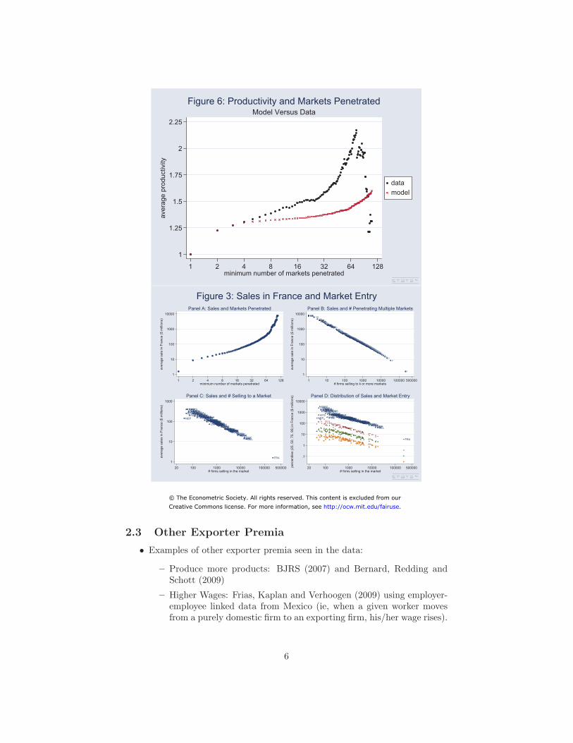
Figure 6: Productivity and Markets Penetrated Model Versus Data

2.25

2

1.75 data model

1.5

1.25

1

1 2 4 8 16 32 64 128 minimum number of markets penetrated

Figure 3: Sales in France and Market Entry Panel A: Sales and Markets Penetrated Panel B: Sales and # Penetrating Multiple Markets

10000 10000 107108109110 106

105101102103104100989997969594919390928988878685838482

aver

age

sale

s in

Fra

nce

($ m

illio

ns)

aver

age

sale

in F

ranc

e ($

mill

ions

)

perc

entil

es (2

5, 5

0, 7

5, 9

5) in

Fra

nce

($ m

illio

ns)

aver

age

sale

in F

ranc

e ($

mill

ions

)

1000

100

10

1000

100

10

81807978777675747372706871696766656463626160585654514948595755535250474645444341424039383736353334323130292827262524232221201918171615141312111098765 4

3 2

1

1 1

1 2 4 8 16 32 64 128 1 10 100 1000 10000 100000 500000 minimum number of markets penetrated # firms selling to k or more markets

Panel C: Sales and # Selling to a Market Panel D: Distribution of Sales and Market Entry 1000 10000

MAW ELSUGABOLNICGUASOMJAMZAMALBSIEPAPHON

MAWUGABOLSIESOMALBAFG JAM VIEELSZAMNICGUA COS1000 VIELIBGHABANSUDETHLIYSRIPARDOMHONCOSLIBGHA

MOZLIYBANTRIPARPAP DOMETHZIMTAN SUDSRI AFG ECU

PANCZEUSRSYRIRNPHIROMINOCHNRWACOLBULANGPAKURUIRQOMANIACHA

MOZZIMBURCUB PERGEEKENGEEECUBURPERCUBIRNKENROM TANTRI VENMAYJORCHITHAMEXARGHUNNEPNEP MAUTURTAIBRAMASNZEINDYUGMALMADKORZAIEGYBUKCENNIGSOUKUWBENSINTOGPHIRWACOLCHNINOBULURUOMAANGPAKUSRPANIRQMAYNIACZE SAUAULIREGREFINSENHOKISRTUNNORJAP100 COTPORDENSWEMORCAMALGAUTCANSPANETITAUNKUSAJORARGCHITHAMEXSYR

EGYVENHUN

KUWMAUTAINZEMASTURYUGKORZAIMADCHA BRAMALINDBUKCENNIG 100

BENSOUSINTOGIRE GERSWIBELAULJAPCANSPA

FINSAUAUT

HOKISRGRESENNORTUNPORCOTDENSWEMORCAMALGNET 10

1

.1

USAUNKITAGERSWIBEL FRA

10

FRA 1

20 100 1000 10000 100000 500000 20 100 1000 10000 100000 500000 # firms selling in the market # firms selling in the market

2.3 Other Exporter Premia

• Examples of other exporter premia seen in the data:

– Produce more products: BJRS (2007) and Bernard, Redding and Schott (2009)

– Higher Wages: Frias, Kaplan and Verhoogen (2009) using employer-employee linked data from Mexico (ie, when a given worker moves from a purely domestic firm to an exporting firm, his/her wage rises).

6

© The Econometric Society. All rights reserved. This content is excluded from ourCreative Commons license. For more information, see http://ocw.mit.edu/fairuse.

– More expensive (‘higher quality’?) material inputs: Kugler and Ver­hoogen (2008) using very detailed data on inputs used by Colombian firms.

– Innovate more: Aw, Roberts and Xu (2008).

– Pollute less: Halladay (2008)

2.3.1 Premia: Selection or Treatment Effects?

• Consider the ‘exporter productivity premium’, which has been found in many, many datasets.

• A key question is obviously whether these patterns in the data are driven by:

– Selection: Firms have exogenously different productivity levels. All firms have the opportunity to export, but only the more productive ones (on average) choose to do so. A fixed cost of exporting delivers this in Melitz (2003), and Bertrand competition delivers this in BEJK (2003).

– Treatment: Somehow, the very act of exporting raises firm produc­tivity. Why?

∗ Intra-industry competition ∗ Exporting to a foreign market (and hence larger total market) allows a firm to expand and exploit economies of scale.

∗ Learning by exporting. ∗ Some exporting occurs through multinational firms, who may have incentives to teach their foreign affiliates how to be more productive.

∗ Focus on ‘core competency’ products (i.e. productivity rise is just selection effect within firm).

• Of course, both of these two effects could be at work.

2.3.2 Premia: Selection or Treatment Effects?

• An important literature has tried to distinguish between these 2 effects:

– Clerides, Lach and Tybout (QJE, 1997)

– Bernard and Jensen (JIE, 1998)

• The conclusion of these studies is that the effect is predominantly selection.

– However, as we shall see below, there is evidence from trade liberal­ization studies of firms becoming more productive after trade liber­alization.

7

– And in more recent work, Trefler and Lileeva (QJE, 2009) and de Loecker (Ecta, 2011) improve upon the methods used in the above papers and find evidence for a treatment effect of exporting on pro­ductivity.

2.4 Firm-level Responses to Trade Liberalization

• An enormous literature has used firm-level panel datasets to explore how firms respond to trade liberalization episodes.

• This has been important for policy, as well as for the development of theory.

– Interestingly, the first available data (and the largest and most plau­sibly exogenous trade liberalization episodes) were from developing countries

– So using firm-level panel data to study trade issues has become an important sub-field in Development Economics (indeed surprisingly, there aren’t that many questions that firm-level data are used to look at in Development other than trade issues!)

2.5 Aggregate Industry Productivity

• Most of these studies have been concerned with the effects of trade liber­alization on aggregate industry productivity.

• Unfortunately, one often cares about much more than this.

– Consumers may care about some industries more than others.

– Within industries, consumers may care about some firms’ varieties more than others’.

– Trade liberalization will also change the set of imported varieties, and this effect is obviously not counted at all in measures of an industry’s (purely domestic) productivity.

– Not all inputs are fully measured, so what one observes as produc­tivity in the data (eg Y/L or TFP) is not true productivity.

– Relatedly, there are probably uncounted adjustment costs behind any liberalization episode.

• Data limitations have presented a full and integrated assessment of all of these channels.

– But there might be ways to make progress here.

– Theory can be particularly informative in shedding light on the mag­nitude of some of these effects.

8

2.5.1 Aggregate Industry Productivity: A Decomposition I

• A helpful way of thinking about the effects of trade liberalization on aggre­gate industry productivity is due to Tybout and Westbrook (1995) among others.

• Notation:

– Output of firm i in year t is: qit = Aitf(vit), where Ait is firm-level TFP and vit is a vector of inputs.

– Let f(vit) = γ(g(vit)), where the function g(.) is CRTS. Then all economies of scale are in γ(.).

– Let Bit = qit/g(vit) be measured productivity. – And let Sit = g(vit)/ i g(vit) be the firm’s market share in its in­

dustry, but where market shares are calculated on the basis of inputs used.

d ln(qit)– And let μit = .d ln(git)

2.5.2 Aggregate Industry Productivity: A Decomposition II • Then industry-wide average productivity (Bt = SitBit) will change i according to: dBt dgit qit Bit

= (μit − 1) + dSitBt git qt Bti i ' -r - ' -r -

Scale effects Between-firm reallocation effects dAit qit +

Ait qti ' -r -Within-firm TFP effects

• The literature here has looked at the extent to which each of these terms responds to a liberalization of trade policy.

2.6 Trade Liberalization

2.6.1 Scale Effects

• Not much work on this.

• But Tybout (2001, Handbook chapter) argues that since exporting plants are already big it is unlikely that there is a large potential for trade to expand underexploited scale economies.

• Likewise, since the bulk of production in any industry is concentrated on already-large firms, the scope for the ‘scale effects’ term to matter in terms of changes is small.

9

2.6.2 Within- and Between-Firm Effects

• This is where the bulk of work has been done.

• Indeed, the finding of significant aggregate productivity gains from between-firm reallocations was an important impetus for work on heterogeneous firm models in trade.

– The finding that reallocations of factors (and market share) from low-Bit to high-Bit firms can be empirically significant was taken by some as evidence for ‘another’ source of welfare gains from trade. (Though this is really just Ricardian gains from trade at work within an industry rather than across industries.)

• However, it is now better recognized that aggregate industry productivity is not equal to welfare and thus one needs to be careful.

– A stark example of this, to my mind, is Arkolakis, Costinot and Rodriguez-Clare (AER, 2011) who show that the Krugman (1980) and Melitz (2003, but with Pareto productivities added) models have exactly the same welfare implications.

– Thus, while the two models seem identical except for the fact that Melitz’s heterogeneous firms create the scope for productivity-enhancing reallocation effects, other welfare effects induced by trade liberaliza­tion go in the opposite direction.

• We will discuss some recent and influential papers in this area.

2.6.3 Pavcnik (ReStud 2002)

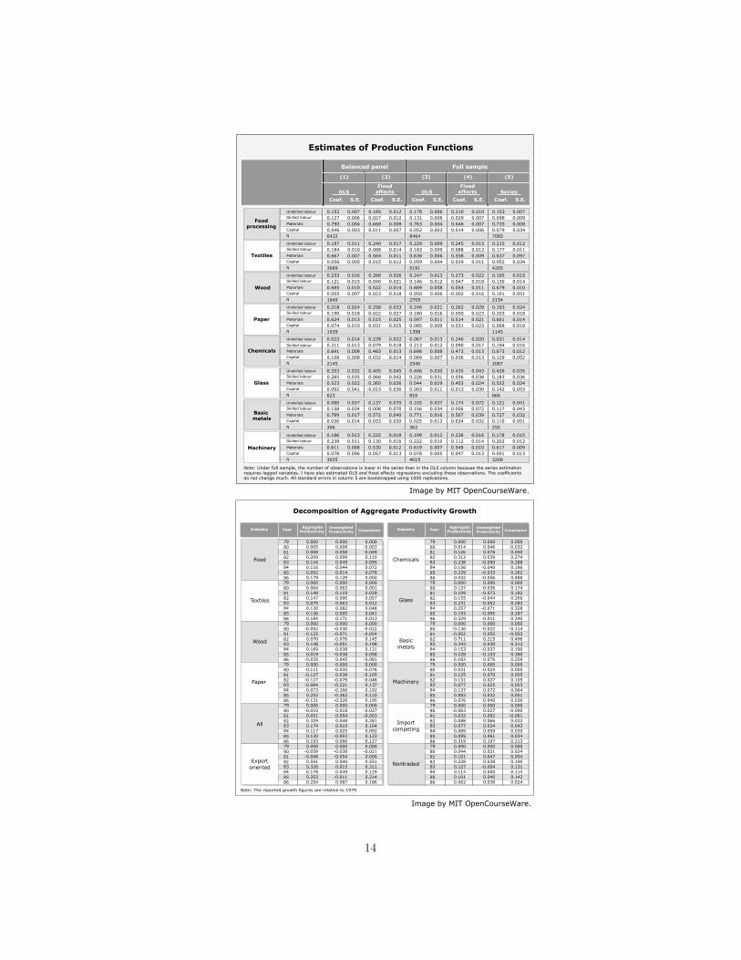
• Pavcnik (2003) recognized that a clear measure of dBt and each of its two Bt Bit dAit qitdecomposition terms i dSit and required a good Bt i Ait qt

measure of Bit.

• It is hard to measure these TFP terms Bit because of:

– Simultaneity: Firms probably observe Bit and take actions (eg how much factor inputs to use) based on it. The econometrician doesn’t observe Bit, but can infer it by comparing outputs to factor inputs used. But this only works if one is careful to ‘reverse-engineer’ the firm’s decisions about factor input choices that were based on Bit.

– Selection: Firms with low Bit might drop out of the sample and thus not be observed to the same extent as high Bit firms.

• Pavcnik (2002) was the first to apply to trade liberalization Olley and Pakes (1996)’s techniques for dealing with simultaneity and selection.

– We discuss this briefly first before returning to the decomposition.

10

∑ ∑

3 Research work that has been done

3.1 Olley and Pakes (Ecta, 1996)

• Drop the firm subscript i (but everything below is at the firm level).

• Let xt be variable inputs that can be adjusted freely, and let kt be capital which takes a period to adjust and is costly to do so (usual convex costs).

• So output is: yt = β0 + βxt + βkkt + ωt + μt, where ωt is TFP that the firm knows and μt is the TFP that the firm does not know. (The econometrician knows neither.) Both are Markov random variables (which is not innocuous actually, since we are trying to estimate TFP in order to relate it to trade policy; is trade policy Markovian?)

• Ericsson and Pakes (1995) show that:

– It is a Markov Perfect Equilibrium for firms to exit unless ωt exceeds some cutoff ωt(kt).

– Investment behaves as: it = it(ωt, kt), where it(.) is strictly increas­ing in both arguments.

• First step: estimate β.

• Estimating β (the coefficient on variable inputs) is easier since we’re as­suming that any firm in the sample in year t woke up in t, observed its ωt, and chose exactly as many variable inputs xt as it wanted.

– Invert it = it(ωt, kt): ωt = θt(it, kt). Note that we have no idea what the function θ(.) looks like.

– Then we have yt = βxt +λt(kt, it)+μt, where λt(kt, it) ≡ β0 +βkkt + θt(kt, it).

– Estimate this function yt and control for λ(.) non-parametrically.

– This is typically done with a ‘series/polynomial estimator’: some high-order (Pavcnik uses 3rd-order) polynomial in kt and it.

– With λt(.) controlled for, the coefficient on xt is just β.

• Second step: estimate βk.

• This is more complicated, as the firm makes an investment decision it in year t that is forward-looking, and this decision determines kt+1. The firms know more about ωt+1 than we do, so we need to worry about this.

– Let the firm’s expectation about ωt+1 be: E [ωt+1|ωt, kt] = g(ωt)−β0. We have no idea what g(.) is, but it should be strictly upward-sloping.

– Note that g(ωt) = g(θt(it, kt)) = g(λt − βkkt). We already have estimates of λt from Step 1 so think of λt as observed.

11

– So we have: yt+1 − βxt+1 = βkkt+1 + g(λt − βkkt) + ξt+1 + μt+1. (ξt+1 is defined by: ξt+1 = ωt+1 − E [ωt+1|ωt, kt].)

– The goal is to estimate βk, which we can do here with non-parametric functions g(.) and non-linear estimation (βk appears inside g(.)).

• However, the above procedure (in Step 2) is invalid if some firms will exit the sample.

– That is, we only observe the firms whose expectations about ωt+1

exceed the continuation cut-off ω (kt).t

• OP (1996) derive another correction for this: – let Pt = Pr(continuing in t+1) = Pr ωt+1 > ωt+1(kt+1)|ωt+1(kt+1), ωt =

pt(ωt, ωt+1(kt+1)). – And let Φ(ωt, ωt+1(kt+1)) = E ωt+1|ωt, ωt+1 > ωt+1(kt+1) + β0.

−1 – So Φ(ωt, ωt+1(kt+1)) = Φ(ωt, p (Pt, ωt)) = Φ(ωt, Pt).t

– Hence we should really estimate yt+1 − βxt+1 = βkkt+1 + Φ(λt − βkkt, Pt) + ξt+1 + μt+1

– This requires an estimate of Pt, the probability of survival. OP show that Pt = pt(it, kt) so we can estimate Pt from a series polynomial probit regression of a survival dummy on polynomials in it and kt.

3.2 Levinsohn and Petrin (ReStud, 2003)

• A limitation of the OP procedure is that it requires investment to be non-zero (recall that it(.) is strictly increasing).

• In the OP model this will never happen, but in the data it does.

– Caballero and Engel and others have done work on models that do include this ‘lumpy investment’.

– Clearly the extent of the problem depends on the length of a ‘period’ t in the data.

– Long periods can mask the lumpy nature of investment but it is probably still a constraint on investment that firms have to worry about).

• Levinsohn and Petrin (2003) introduce a procedure for dealing with this (but Pavcnik doesn’t use it).

3.3 Pavcnik (2002): Data and Setting

• Chile’s trade liberalization:

– Began in 1974, finished by 1979. (Tariffs actually rose a bit in 1982 and 1983 before falling again).

12

– As usual with these trade liberalization episodes, there were a lot of other things going on at the same time.

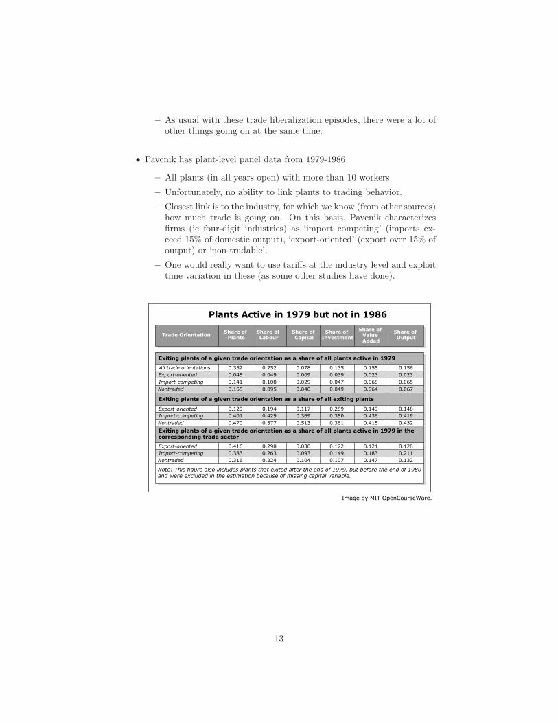
• Pavcnik has plant-level panel data from 1979-1986

– All plants (in all years open) with more than 10 workers

– Unfortunately, no ability to link plants to trading behavior.

– Closest link is to the industry, for which we know (from other sources) how much trade is going on. On this basis, Pavcnik characterizes firms (ie four-digit industries) as ‘import competing’ (imports ex­ceed 15% of domestic output), ‘export-oriented’ (export over 15% of output) or ‘non-tradable’.

– One would really want to use tariffs at the industry level and exploit time variation in these (as some other studies have done).

13

Trade OrientationShare of

PlantsShare of Labour

Share of Capital

Share of Investment

Share of Value Added

Share of Output

Exiting plants of a given trade orientation as a share of all plants active in 1979

All trade orientationsExport-oriented

Import-competingNontraded

0.352 0.252 0.078 0.135 0.155 0.1560.045 0.049 0.009 0.039 0.023 0.023

0.141 0.108 0.029 0.047 0.068 0.0650.165 0.095 0.040 0.049 0.064 0.067

Exiting plants of a given trade orientation as a share of all exiting plants

Export-orientedImport-competingNontraded

0.129 0.194 0.117 0.289 0.149 0.1480.401 0.429 0.369 0.350 0.436 0.4190.470 0.377 0.513 0.361 0.415 0.432

Exiting plants of a given trade orientation as a share of all plants active in 1979 in the corresponding trade sector

Export-orientedImport-competingNontraded

0.416 0.298 0.030 0.172 0.121 0.1280.383 0.263 0.093 0.149 0.183 0.2110.316 0.224 0.104 0.107 0.147 0.132

Note: This figure also includes plants that exited after the end of 1979, but before the end of 1980and were excluded in the estimation because of missing capital variable.

Plants Active in 1979 but not in 1986

Image by MIT OpenCourseWare.

14

Unskilled labour

Skilled labour

Materials

Capital

N

Unskilled labour

Skilled labour

Materials

Capital

N

Unskilled labour

Skilled labour

Materials

Capital

N

Unskilled labour

Skilled labour

Materials

Capital

N

Unskilled labour

Skilled labour

Materials

Capital

N

Unskilled labour

Skilled labour

Materials

Capital

N

Unskilled labour

Skilled labour

Materials

Capital

N

Unskilled labour

Skilled labour

Materials

Capital

N

0.152 0.007 0.185 0.012 0.178 0.006 0.210 0.010 0.153 0.0070.127 0.006 0.027 0.012 0.131 0.006 0.029 0.007 0.098 0.0090.790 0.004 0.668 0.008 0.763 0.004 0.646 0.007 0.735 0.0080.046 0.003 0.011 0.007 0.052 0.003 0.014 0.006 0.079 0.0346432 8464 7085

0.187 0.011 0.240 0.017 0.229 0.009 0.245 0.015 0.215 0.0120.184 0.010 0.088 0.014 0.183 0.009 0.088 0.012 0.177 0.0110.667 0.007 0.564 0.011 0.638 0.006 0.558 0.009 0.637 0.0970.056 0.005 0.015 0.012 0.059 0.004 0.019 0.011 0.052 0.0343689 5191 4265

0.233 0.016 0.268 0.026 0.247 0.013 0.273 0.022 0.195 0.0150.121 0.015 0.040 0.021 0.146 0.012 0.047 0.018 0.130 0.0140.685 0.010 0.522 0.014 0.689 0.008 0.554 0.011 0.679 0.0100.055 0.007 0.023 0.018 0.050 0.006 -0.002 0.016 0.101 0.0511649 2705 2154

0.218 0.024 0.258 0.033 0.246 0.021 0.262 0.029 0.193 0.0240.190 0.018 0.022 0.027 0.180 0.016 0.050 0.023 0.203 0.0180.624 0.013 0.515 0.025 0.597 0.011 0.514 0.021 0.601 0.0140.074 0.010 0.031 0.025 0.085 0.009 0.031 0.023 0.068 0.0181039 1398 1145

0.033 0.014 0.239 0.022 0.067 0.013 0.246 0.020 0.031 0.0140.211 0.013 0.079 0.018 0.213 0.012 0.090 0.017 0.194 0.0160.691 0.009 0.483 0.013 0.698 0.008 0.473 0.013 0.673 0.0120.108 0.008 0.032 0.014 0.089 0.007 0.036 0.013 0.129 0.0522145 2540 2087

0.353 0.032 0.405 0.045 0.406 0.030 0.435 0.043 0.426 0.0350.285 0.035 0.068 0.042 0.226 0.031 0.056 0.038 0.183 0.0360.523 0.022 0.360 0.026 0.544 0.019 0.403 0.024 0.522 0.0240.092 0.041 -0.015 0.036 0.093 0.011 -0.013 0.030 0.142 0.053623 816 666

0.080 0.037 0.137 0.070 0.105 0.037 0.174 0.072 0.121 0.0410.158 0.034 0.008 0.070 0.156 0.034 0.006 0.072 0.117 0.0430.789 0.017 0.572 0.040 0.771 0.016 0.567 0.039 0.727 0.0320.030 0.014 0.033 0.030 0.025 0.013 0.034 0.032 0.110 0.051306 362 255

0.186 0.013 0.225 0.018 0.199 0.012 0.238 0.016 0.178 0.0150.238 0.011 0.130 0.016 0.222 0.010 0.112 0.014 0.202 0.0120.611 0.008 0.530 0.012 0.619 0.007 0.548 0.010 0.617 0.0090.078 0.006 0.057 0.013 0.078 0.005 0.047 0.013 0.051 0.0133025 4015 3268

Coef. S.E. Coef. S.E. Coef. S.E. Coef. S.E. Coef. S.E.

OLSFixed

effects OLSFixed

effects Series

Balanced panel Full sample

Foodprocessing

Textiles

Wood

Paper

Chemicals

Glass

Basic metals

Machinery

Note: Under full sample, the number of observations is lower in the series than in the OLS column because the series estimation requires lagged variables. I have also estimated OLS and fixed effects regressions excluding these observations. The coefficients do not change much. All standard errors in column 5 are bootstrapped using 1000 replications.

Estimates of Production Functions

(1) (2) (3) (4) (5)

Industry YearAggregate

Productivity UnweightedProductivity Covariance

798081828384858679808182838485867980818283848586798081828384858679808182838485867980818283848586

0.0000.0140.1260.3120.2380.1560.2290.4320.0000.1370.1090.1550.2310.2570.1930.3290.000

-0.136-0.0020.7110.3430.1530.228

0.000

0.1250.031

0.1310.0770.1370.0830.0760.000

-0.0630.0320.0880.0770.0890.0950.3190.0000.0440.1010.2280.1270.1140.1010.062

0.0000.0460.0760.039

-0.050-0.040-0.033-0.0560.000

-0.036-0.073-0.044-0.052-0.071-0.095-0.0110.000

-0.0220.0500.2150.030

-0.037-0.153

0.000

0.070-0.025

0.0270.0250.0720.0320.0400.0000.0270.0920.0660.0340.0590.0610.1070.0000.0210.0470.038

-0.0040.0000.0400.038

0.000-0.0320.0500.2740.2880.1960.2620.4880.0000.1740.1820.2000.2830.3280.2870.3400.000

-0.114-0.0520.4960.3120.1900.380

0.183 0.076 0.2590.000

0.0550.005

0.1050.0530.0640.0510.0360.000

-0.090-0.0610.0220.0430.0300.0340.2130.0000.0240.0540.1900.1310.1140.1420.024

798081828384858679808182838485867980818283848586798081828384858679808182838485867980818283848586

0.0000.0050.0080.2090.1440.1160.0920.1790.0000.0640.1480.1470.0750.1300.1360.1840.000

-0.052-0.1250.0700.1480.1690.019

0.000

-0.127-0.111

-0.127-0.084-0.0730.252

-0.1310.000

-0.0100.0510.3290.1740.1170.1200.1930.000

-0.059-0.0480.5910.3260.1780.2030.254

0.0000.0080.0580.0990.0490.0440.0140.1290.0000.0630.1190.0900.0630.0820.0950.1710.000

-0.030-0.071-0.076-0.0510.038

-0.038

0.000

0.038-0.035

-0.079-0.221-0.266-0.362-0.3260.0000.0180.0540.0480.0100.025

-0.0030.0660.000

-0.038-0.0540.0400.0150.049

-0.0110.087

0.000-0.003-0.0490.1100.0950.0720.0780.0500.0000.0010.0290.0570.0120.0480.0410.0130.000

-0.022-0.0540.1450.1980.1310.058

-0.035 0.045 -0.0810.000

-0.165-0.076

-0.0480.1370.1920.1100.1950.000

-0.027-0.0030.2810.1640.0920.1230.1270.000

-0.0210.0060.5510.3110.1290.2140.166

Food

Textiles

Wood

Paper

All

Exportoriented

Chemicals

Glass

Basicmetals

Machinery

Importcompeting

Nontraded

Note: The reported growth figures are relative to 1979.

Industry YearAggregate

Productivity UnweightedProductivity Covariance

Decomposition of Aggregate Productivity Growth

Image by MIT OpenCourseWare.

Image by MIT OpenCourseWare.

3.4 Trefler (AER, 2004)

• Trefler evaluates how Canadian industries and plants responded to Canada’s trade agreement with the United States in 1989.

• This is a particularly ‘clean’ trade liberalization (not a lot of other com­ponents of some broader ‘liberalization package’ as was often the case in developing country episodes).

• Further, this is a rare example in the literature of a reciprocal trade agree­ment:

– Canada lowered its tariffs on imports from the US, so Canadian firms in import-competing industries face more competition.

– And the US lowered its tariffs on Canadian imports, so Canadian firms in export-oriented industries face lower costs of penetrating US markets.

• So this is a great ‘experiment’. Unfortunately the data aren’t as rich as Pavcnik’s so Trefler can’t look at everything he’d like to.

15

Export-oriented

Import-competing

ex_80

ex_81

ex_86

R2 (adjusted)

Year indicators

Plant indicators

Industry indicators

Exit_import indicator

Exit_export indicator

Exit indicator

im_86

im_85

im_84

im_83

im_82

im_81

im_80

ex_85

ex_84

ex_83

ex_82

N

0.106

22983

0.057

No

Yes

Yes

-0.081

0.103

0.062

0.042

0.033

0.047

0.011

0.030

0.050

0.021

0.005

-0.099

-0.054

0.105

0.030**

0.032

0.032

0.031

0.030 0.031 0.030

0.036

0.014

0.011**

0.023

0.036

0.014**

0.017**

0.017**

0.017**

0.017**

0.017**

0.017**

0.017**

0.019**

0.017**

0.017**

0.017** 0.016*0.016**

0.015**

0.014 0.014

0.015** 0.015**

0.025**

0.028**

0.021**

0.030** 0.031** 0.048** 0.048** 0.046**

0.010**

0.015*

0.015** 0.015**0.015**

0.015** 0.015**

0.015**

0.017**

0.015** 0.016**

0.014**

0.015* 0.015*

0.035*

0.021

0.015**

0.014** 0.014**

0.028 0.028

0.029 0.030 0.029

0.0290.030

0.013

0.029

0.028* 0.028

0.028

0.014

0.034

0.027** 0.027**

0.028*

0.026** 0.026**

0.027**

0.026**

0.032

0.032

0.031

0.025**

0.028**

0.021**

0.032

0.032

0.031

0.025**

0.028**

0.021**

Yes

No

Yes

Yes

No

Yes

Yes

Yes

Yes

-0.007

-0.021

-0.076

0.104

0.062

0.043

0.034

0.047

0.011

0.032

0.051

0.023

0.007

-0.097

-0.053

0.105

0.106

0.071

0.104

0.063

0.043

0.030

0.046

0.010

0.043

0.028

0.050

0.021

0.003

-0.100

-0.055

0.103

0.112

22983 25491 22983

0.058 0.062 0.498

Yes

Yes

Yes

Yes

Yes

Yes

22983 25491

0.498 0.488

0.098

-0.024

-0.019

0.101

0.059

0.040

0.024

0.044

0.013

-0.001

0.007

-0.036

-0.054

-0.117

-0.071

0.040 0.040 0.039

0.014 0.014

0.013

0.013

-0.005

-0.069

-0.010

0.102

0.059

0.041

0.024

0.044

0.017

-0.025

-0.042

-0.110

-0.068

-0.025

0.095 0.100

0.073

0.101

0.061

0.042

0.025

0.044

0.013

-0.008

-0.003

0.007

-0.038

-0.055

-0.119

-0.071

-0.007

Coef. S.E. Coef. S.E. Coef. S.E. Coef. S.E. Coef. S.E. Coef. S.E.

(1) (2) (3) (4) (5) (6)

Estimates of Equation 12

Note: ** and * indicate significance at a 5% and 10% level, respectively. Standard errors are corrected for heteroscedasticity. Standard errors in columns1_3 are also adjusted for repeated observations on the same plant. Columns 1, 2, 4, and 5 do not include observations in 1986 because one cannot defineexit for the last year of a panel.

Image by MIT OpenCourseWare.

3.4.1 Empirical Approach

• Define the policy ‘treatment’ variables:

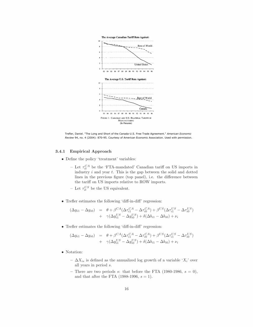
– Let τ CA be the ‘FTA-mandated’ Canadian tariff on US imports in it industry i and year t. This is the gap between the solid and dotted lines in the previous figure (top panel), i.e. the difference between the tariff on US imports relative to ROW imports.

– Let τUS be the US equivalent. it

• Trefler estimates the following ‘diff-in-diff’ regression:

θ + βCA(ΔτCA − Δτ CA) + βUS(ΔτUS − ΔτUS(Δyi1 − Δyi0) = )i1 i0 i1 i0 US US+ γ(Δy − Δy ) + δ(Δbi1 − Δbi0) + νii1 i0

• Trefler estimates the following ‘diff-in-diff’ regression:

θ + βCA(ΔτCA − Δτ CA) + βUS(ΔτUS − ΔτUS(Δyi1 − Δyi0) = )i1 i0 i1 i0 US US+ γ(Δy − Δy ) + δ(Δbi1 − Δbi0) + νii1 i0

• Notation:

– ΔXis is defined as the annualized log growth of a variable ‘Xi’ over all years in period s.

– There are two periods s: that before the FTA (1980-1986, s = 0), and that after the FTA (1988-1996, s = 1).

16

Trefler, Daniel. "The Long and Short of the Canada-U.S. Free Trade Agreement." American EconomicReview 94, no. 4 (2004): 870-95. Courtesy of American Economic Association. Used with permission.

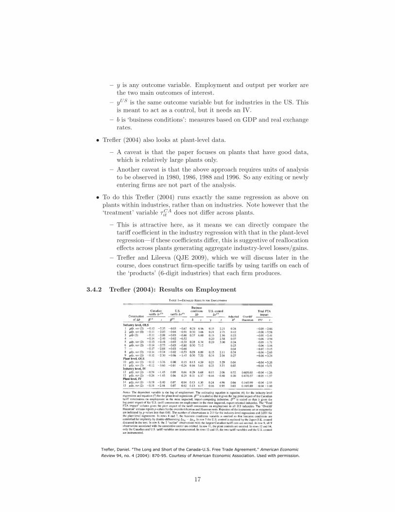
– y is any outcome variable. Employment and output per worker are the two main outcomes of interest. US– y is the same outcome variable but for industries in the US. This

is meant to act as a control, but it needs an IV.

– b is ‘business conditions’: measures based on GDP and real exchange rates.

• Trefler (2004) also looks at plant-level data.

– A caveat is that the paper focuses on plants that have good data, which is relatively large plants only.

– Another caveat is that the above approach requires units of analysis to be observed in 1980, 1986, 1988 and 1996. So any exiting or newly entering firms are not part of the analysis.

• To do this Trefler (2004) runs exactly the same regression as above on plants within industries, rather than on industries. Note however that the ‘treatment’ variable τCA does not differ across plants. it

– This is attractive here, as it means we can directly compare the tariff coefficient in the industry regression with that in the plant-level regression—if these coefficients differ, this is suggestive of reallocation effects across plants generating aggregate industry-level losses/gains.

– Trefler and Lileeva (QJE 2009), which we will discuss later in the course, does construct firm-specific tariffs by using tariffs on each of the ‘products’ (6-digit industries) that each firm produces.

3.4.2 Trefler (2004): Results on Employment

17

Trefler, Daniel. "The Long and Short of the Canada-U.S. Free Trade Agreement." American EconomicReview 94, no. 4 (2004): 870-95. Courtesy of American Economic Association. Used with permission.

3.5 Subsequent Work: de Loecker (Ecta, 2011)

• A well-known (and probably severe) problem with measuring productivity is that we rarely observe output yit properly.

– Instead, in most settings, one sees revenues/sales rit at the plant level but some price measure only at the industry level: pt.

• Klette and Griliches (1995) show the consequences of this:

– What we think is a measure of firm-level TFP (eg yit/g(vit)) is re­ally a mixture of firm-level TFP, firm-level mark-ups, and firm-level demand-shocks.

• This is bad for studies of productivity. But it is worse for studies like Pavcnik (2002) above that want to relate economic change (like trade liberalization) to changes in productivity.

– Economic change (including trade liberalization) may change mark­ups and demand.

– Indeed, theory such as BEJK (2003) and Melitz and Ottaviano (ReStud, 2008) suggests that mark-ups will change.

– And Tybout (2000, Handbook chapter) reviews evidence of mark-ups (and profit margins) changing.

– de Loecker and Warzynski (AER 2012) extend Hall’s (1988) method for measuring mark-ups and finds that they differ by firm trading status.

18

Trefler, Daniel. "The Long and Short of the Canada-U.S. Free Trade Agreement." American EconomicReview 94, no. 4 (2004): 870-95. Courtesy of American Economic Association. Used with permission.

3.6 de Loecker (2010)

• One natural solution would be to work in settings where we do observe good firm-level price data. But this is quite hard.

• de Loecker (2010) proposes a more model-driven solution:

– He specifies a demand system (CES across each firm’s variety, plus firm-specific demand shifters).

– This leads to an estimating equation like that used in OP (1996), but with two complications.

– First, each firm’s demand-shifter appears on the RHS. He effectively instruments for these using trade reform variables (quotas, in a set­ting of Belgian textiles).

– Scond, Each coefficient (eg βk on capital) is no longer the production function parameter, but rather the production function parameter times the markup. But there is a way to correct for this after estimat­ing another coefficient (that on total industry quantity demanded) which is the CES taste parameter (from which one can infer the markup).

• de Loecker finds that the measured productivity effects of Belgium’s textile industry reform fall by 50% if you use his method compared to the pure OP (ie Pavcnik) method.

4 Possible Ideas for Future Work

• On the export premium: what is so special (if anything) about goods crossing international borders?

• Can we do firm-level studies that pay attention to and estimate GE effects?

• Do the ‘exporting is rare’ or ‘exporters are different’ stylized facts change our interpretation of existing Ricardian or HO trade studies?

• Can firm-level studies shed light on the importance of CA vs IRTS in driving trade?

• Estimate trade liberalizations with a stronger connection to welfare (not just pure productivity).

• Could some new empirical IO tools (to study competition, interaction, demand systems, entry models, multiple equilibria) improve our approach to trade problems at the firm-level?

• How does trade affect (or behave in an environment of) misallocations (a la Hseih and Klenow (QJE, 2009))?

19

MIT OpenCourseWarehttp://ocw.mit.edu

14.581International Economics ISpring 2013

For information about citing these materials or our Terms of Use, visit: http://ocw.mit.edu/terms.