“minimum wages and informal employment in developing...
TRANSCRIPT
Minimum Wages and Informal Employment in DevelopingCountries ∗
Giulia Lotti†1, Julian Messina‡1,3 and Luca Nunziata§2,3
1Inter-American Development Bank2University of Padua
3IZA
August 24, 2016
Abstract
We present new empirical evidence on the implications of minimum wages on informalemployment in developing countries, analyzing a unique dataset assembled from a setof micro surveys collected in 59 low and middle income countries. Our identificationstrategy exploits relative bindingness in minimum wages across labor market groups withincountries. The empirical findings show that a higher minimum wage is associated witha larger self-employment share. The effect is approximately linear in the relative level ofthe minimum wage, even if higher levels of minimum wages are associated with higherlevels of non-compliance. The estimated impact of the minimum wage on informalityis economically significant: a 1 percentage point increase in the minimum wage ratio isassociated with a 0.204 percentage points increase in the self-employment rate.
Keywords: Minimum Wage, Informal Jobs, Self-Employment, Developing Countries.
JEL Codes: J38, O17, J21.
∗We thank the World Bank for its financial support and the opportunity to access the International IncomeDistribution (I2D2) data set; the International Labour Organization Global for its kind assistance in using theILO Global Wage dataset, and Kristen Sobeck in particular; and seminar participants to the 18th IZA EuropeanSummer School in Labor Economics for comments and suggestions. The usual disclaimer applies.†[email protected]‡[email protected]§[email protected]
1
1 Introduction
Minimum wages are perhaps the most popular labor market policy tool in developing coun-
tries. The motivations for raising minimum wages are various, reducing inequality and fighting
poverty being commonly held rationales. However, the potential for the minimum wage in
achieving these goals may be hampered by informality. If workers in the formal sector are
pushed into informal jobs as a consequence of the minimum wage hike, the impacts of the min-
imum wage on inequality and/or poverty may be nil, or even negative. As of today, there is no
consensus in the empirical literature regarding the impact of the minimum wage on informality
in the developing world.
This lack of consensus possibly rests on two complementary explanations. The largest
fraction of the literature has focused on analyzing the effects of minimum wage legislation in
advanced economies (Neumark & Wascher, 1992; Card, 1992; Dickens et al., 1999; Dube et al.,
2010; Draca et al., 2011; Addison & Ozturk, 2012; Addison et al., 2013; Neumark et al., 2014).
The literature studying the impacts of the minimum wage in developing countries is instead
sparser, and has mostly focused on Latin American economies. In addition, even among middle
income countries, existing evidence is inconclusive. Large negative effects of the minimum wage
on formal employment are found in Honduras (Gindling & Terrell, 2009), but in Costa Rica
(Gindling & Terrell, 2007), Colombia (Maloney et al., 2001) and Vietnam (Nguyen Viet, 2010)
the effects are small, and not statistically significant in Mexico (Bell, 1997), Brazil (Lemos,
2009) and Thailand (Del Carpio et al., 2014).
The minimum wage may have heterogeneous effects across countries, possibly depending
on interactions with other labor market policies and structural features of the labor market.
An important source of heterogeneity that is often ignored in the literature is how binding the
minimum wage is. For example, in Mexico the minimum wage is relatively low, at 29 percent
of the 70th percentile of the wage distribution in the formal sector. In Colombia instead, the
minimum wage is more generous (64 percent of the 70th wage percentile), and above the median
for certain labor market groups (e.g. young and low educated workers). If the impact of the
minimum wage kicks-in only after a certain threshold, some of these apparent contradictory
results may be reconciled.
2
This paper presents new evidence on the impact of the minimum wage on informality by
assembling a unique dataset of micro surveys from 59 middle income developing countries
observed in the period 1995-2012. In our baseline specification, informality is measured as the
share of self-employed and family workers, i.e. those workers who are by definition not covered
by minimum wage legislation, on total employment outside of agriculture. In addition, we
present a series of robustness checks using alternative definitions of informal workers.
Assessing the impact of the minimum wage across countries, or within countries over time,
may be problematic because other labor market policies and macro shocks may be correlated
with changes in the minimum wage legislation. Instead, our empirical strategy, in the spirit of
Rajan & Zingales (1998), consists in contrasting the relative effectiveness of the minimum wage
across labor market groups within countries and years. The interaction between the typical
wage attaining to a specific labor market group and the country/year minimum wage setting
is informative about the relative bite of the minimum wage policy across groups, and we use
such variation in the data to estimate how minimum wages affect informality. For some groups
(e.g. young female with basic education and young male with basic education) minimum wage
policies may be more binding and therefore the effect on informality may be relatively stronger.
Our approach relies on an implicit identifying assumption, namely that variations in min-
imum wage levels do not affect the shape of the underlying wage distribution for each labor
market group. Our strategy therefore resembles that of Lee (1999), who assesses the impact of
the federal minimum wage on US wage inequality using the variation in the relative bite of the
minimum wage across US states.
Our analysis is based on a unique newly assembled pooled individual-level dataset covering
59 developing countries and investigates the effectiveness of the minimum wage for a set of
twelve labor market groups defined on the basis of individual age, gender and level of education
in each country and year. The effectiveness of the minimum wage is calculated as the ratio of
the country/year minimum wage to the 70th percentile of formal sector wages in each group.
We call this variable the minimum wage ratio. Such a high percentile in the wage distribution is
unlikely to be affected by minimum wages, but we provide robustness checks for different cut-off
points. This rich data set allows us to analyze not only the average effect of the minimum wage
on informality, but also whether the impact is heterogeneous across country groups.
3
We also investigate possible non-linearities in the impact of the minimum wage on informal-
ity. Indeed, informality does not need to be an exclusion state. It may instead be a worker’s
choice, either because the worker does not appreciate enough the amenities of a formal job
(e.g. a right to a pension or health insurance) or because she values as highly desirable certain
attributes of the informal job (e.g. greater flexibility in working hours). Empirical evidence
against labor market segmentation has been found in several Latin American countries (see
Maloney, 1999 and Bosch & Maloney, 2010). In this context, if minimum wages are sufficiently
low (i.e., close to the market wage) they may have no effects on formality, or the effects may
be even positive if they provide sufficient incentives for workers to accept a formal job. If the
minimum wage is instead relatively high with respect to the underlying worker productivity, the
disincentive effect on job creation is likely to more than compensate for the increased worker’s
willingness to take a formal job.1 Hence, different stringency levels of the minimum wage with
respect to market wages may have different consequences on informality.
Our estimates show that a higher minimum wage is associated with a larger share of self-
employment. Our estimated effects are not modest: our baseline model indicates that a one
standard deviation increase in the minimum wage ratio raises informality by 18.25 percent.
Interestingly, the estimated effect appears fairly linear, with higher minimum wages having a
larger negative effect on formal employment.
We acknowledge and document the substantial heterogeneity across countries regarding the
coverage of the minimum wage laws, which often vary across sectors (e.g. excluding agriculture),
occupations (e.g. high vs. low skilled), workers’ age (e.g. young and apprentices vs. prime-aged)
and geographical coverage (e.g. nation-wide vs. regional or provincial). However, a battery of
robustness checks suggests that such heterogeneity has a small impact on the estimated results.
The paper is organized as follows. Section 2 introduces the identification strategy, section 3
provides a description of the data, section 4 presents the empirical findings, section 5 includes
robustness checks, and section 6 concludes.
1See Brown et al. (2014) for a similar discussion in the context of the impact of the minimum wage onemployment.
4
2 Research Design
We investigate the implication of different levels of minimum wage stringency on a measure of
informality, i.e. the share of self-employment plus family workers in total employment outside
of agriculture. Our identification strategy is close to Rajan & Zingales (1998) and is built
on the assumption that minimum wage legislation is likely to be more binding for specific
labour market groups according to their wage distribution. Certain labour market groups may
be confronted with stronger rigidities and hence larger behavioural responses and effects on
economic outcomes. As a consequence, if the minimum wage has an impact on informality,
it will be larger among labour market groups whose typical wage is closer to the minimum
wage threshold. We identify the impact of the minimum wage on informality by exploiting
such different levels of effectiveness of the minimum wage across different labor market groups.
This research design allows to control for all aggregate factors that are, on average, unlikely to
have a different effect on informality among labour market groups. These are all country/year
unobservable factors and other potential determinants of informality that are country/year
specific.
Our baseline estimates are obtained using a unique individual-level dataset collected across
59 developing countries. Our model specifications rely on individual data in which the de-
pendent variable is a binary indicator for employed workers who are self-employed or family
workers, and our variable of interest varies across country/year/labor market group dimensions.
In all our specifications we cluster the standard errors at the group level to avoid over-stating
the precision of the estimates (Colin Cameron & Miller, 2015).
We define labor market groups by country/year on the basis of workers’ age, gender, and
education. For each cell, i.e. country/year/group, observation we calculate a measure of the
effectiveness of the minimum wage. Following (Lee, 1999), we define the strictness of the
minimum wage, as the ratio of the prevailing minimum wage in a country/year and some
measure of centrality (or location) of wages for each labor market group. (Lee, 1999) uses the
median wage as an indicator of location. The underlying assumption is that the median is
unaffected by the minimum wage, and hence provides a valid benchmark against which one can
assess how stringent the minimum wage is. However, minimum wages in developing countries
5
close to or even above median wages are not rare, in particular for young, female and less
educated workers. To limit possible spillover effects of the minimum wage into our measure of
centrality our benchmark specification uses the 70th percentile of the group-specific distribution
of wages as a measure of location. In robustness checks we show that variations in the measure
of centrality do not affect the results.
The choice of the dimensions that define the labor market groups is subject to a trade-off
between having a large number of cells with few individuals per cell (with imprecise estimates of
the appropriate minimum wage ratio by cell) and a smaller number of cells with more individuals
and therefore more precise estimates of the minimum wage ratio. Labor market groups should
be chosen in order to have homogeneous individuals within each cell to minimize the variance of
the measurement error when calculating the average minimum wage’s stringency across groups.
In addition, cells should be sufficiently heterogeneous with enough between variation in order
to obtain more precise estimates of the parameter of interest.
Our model will adopt robust standard errors in order to account for the heteroskedasticity
arising from the difference in the precision of the calculation of averages of cells of different
sizes. In the baseline specifications we consider a total of 12 possible groups by interacting
gender with three age groups (16-29; 30-59; 50-65) and two education levels (primary or less
and more than primary). We use primary education as a threshold because, while progress
towards universal primary school completion has been made in many developing countries,
access to secondary education is still far from being granted to the most vulnerable.
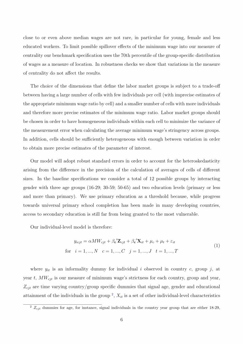
Our individual-level model is therefore:
yicjt = αMWcjt + βc′Zcjt + βc
′Xit + µc + µt + εit
for i = 1, ..., N c = 1, ..., C j = 1, ..., J t = 1, ..., T(1)
where yit is an informality dummy for individual i observed in country c, group j, at
year t, MWcjt is our measure of minimum wage’s strictness for each country, group and year,
Zcjt are time varying country/group specific dummies that signal age, gender and educational
attainment of the individuals in the group 2, Xit is a set of other individual-level characteristics
2 Zcjt dummies for age, for instance, signal individuals in the country year group that are either 18-29,
6
3 and µc and µt are, respectively, country and year fixed effects.
The effects of the minimum wage on informality is therefore estimated by controlling for
country, group and time unobservable dimensions. Our research design therefore resembles
that of an experiment where the definition of a minimum wage level at the country, region or
sectoral level would impose alternative minimum wage stringency levels across cells on the basis
of their representative 70th wage percentile.
Since each cell in our setting represents a variation in the minimum wage stringency level
of equal importance, our baseline individual-level estimates are weighted in order to give equal
weight to each cell4 in order to avoid a bias induced by the difference in relative numerosity of
each cell.
Group level averages are likely to be characterized by sampling error in finite samples if the
cell size is too small. In our setting this may induce a measurement error in our measure of
the minimum wage ratio by cell (i.e. country/group/year) and induce a bias in our estimates.
Since the cell size is inversely proportional to the number of cells used in the analysis, and
a lower number of cells CJT increases the variance of the estimator, then the problem that
the researcher faces in this case is typically a trade-off between bias and variance. According
to Verbeek & Nijman (1992, 1993) and Nunziata (2015) a cell size of 100 should typically
eliminate the bias in a setting like ours. In what follows, we adopt a minimum cell dimension
of 100 individuals and perform some robustness checks adopting cells of different sizes. One
element that we have to bear in mind is that dropping those cells whose dimension is smaller
than the adopted minimum threshold may also introduce a selection bias in our estimates. All
these aspects are discussed in detail in the empirical findings section.
30-50 or 51-653Xit indicate whether the invidual lives in an urban area, whether he/she is the head of the household,
his/her household size and the sector in which he/she works4The weight to each individual observation is equal to 1 over the number of observations in the cell.
7
3 The Data
Our estimations are performed on a rich and unique newly assembled dataset covering 59
developing countries. We use two main sources to construct it. The first consists in the new
International Income Distribution (I2D2 henceforth) data set, a global harmonized household
survey database created by the World Bank that allows us to compare different countries around
the world and across time. The vast majority of the surveys included in the I2D2 are nation-
ally representative (World Bank, 2013). The dataset is extremely rich and comprehensive in
coverage, but it is also noisy, as it collects data from surveys that were not designed to be
comparable. Our empirical strategy limits the impact of these flaws by restricting the identifi-
cation to comparisons across groups within country/year waves, i.e., by effectively eliminating
variation across countries or within countries over time.
We merge the I2D2 with the International Labor Organization Global Wage dataset (Inter-
national Labour Office (ILO), 2013), which covers statutory nominal gross monthly minimum
wage levels effective December 31st across the world. We use the ILO dataset to build indicators
of the effectiveness of the minimum wage across 12 different labor market groups based on the
interaction of individual-level information on gender, age (three age groups: 18-29, 30-50 and
51-65) and education (primary or less and more than primary). These groups are therefore:
female/male between 18 and 29 years old who are low/highly educated, female/male between
30 and 50 years old who are low/highly educated, female/male between 51 and 65 years old
who are low/highly educated.
While constructing the dataset, we checked for discrepancies in the distribution of wages
and minimum wages. In some cases minimum wages are at odds with the wage distribution
in the country/year. This is possibly due to measurement errors in one of the two databases
or problems with the units of measurement in the I2D2 that could not be solved. For further
details please refer to Appendix A in section 6. After dropping these problematic waves we are
initially left with 63 countries and 332 survey waves.
As we want to focus our attention on the share of self-employed outside agriculture, we
exclude the individuals who work in this sector because in most countries the minimum wage
does not apply to it. We drop cells where the share of self-employed outside of agriculture
8
seems to be zero; we are left with 330 waves corresponding to 62 countries. 5
We then exclude one wave that shows some problems in the variables: Tanzania 2009 (many
values of industry agriculture, mining, manufacturing, public utilities - are missing). We are
left with 329 waves relative to 62 countries and 727 country/groups, corresponding to 3,850
country/year/group observations (i.e. cells). In order to derive meaningful measures of the
effectiveness in the minimum wage we include in the empirical analysis only those cells with at
least 100 observations. This way we also drop the Russian Federation and we are left with 61
countries, 321 waves and 2,730 cells.
We can also exclude observations for which the minimum wage ratio over the 70th percentile
wage is strictly greater than one, because this may indicate a disproportioned rate of non
compliance, and our identification strategy may be compromised in this case.6. We also exclude
observations for which control variables exhibit missing values. We are left with 59 countries,
311 waves and 2,361 cells, for a total of 16,112,765 individuals, of which 9,482,235 are employed.
Further details about the dataset construction can be found in the Appendix.
Finally, in order to provide a set of estimates on country subsamples defined on whether the
rule of law is above or below the world median, we use the Rule of Law Indicator from the World
Bank Worldwide Governance Indicators (WGI). The Rule of Law index “captures perceptions
of the extent to which agents have confidence in and abide by the rules of society, and in
particular the quality of contract enforcement, property rights, the police, and the courts, as
well as the likelihood of crime and violence. Estimate gives the country’s score on the aggregate
indicator, in units of a standard normal distribution, i.e. ranging from approximately -2.5 to
2.5” (World Bank, WGI).
FIGURE 1 AROUND HERE
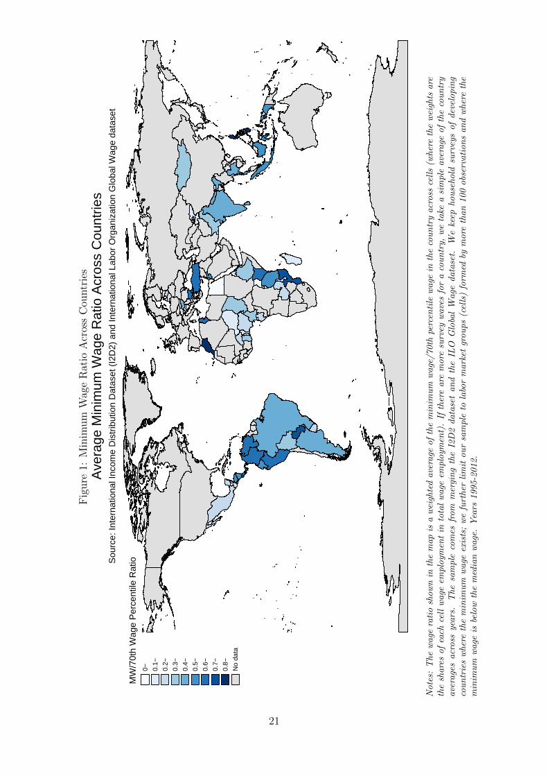
Figure 1 displays the country coverage in our sample and the average minimum wage ratio
across countries. The latter is characterized by a significant variability across countries. Coun-
tries where the minimum wage is more binding across groups and time are mainly from the
5In the only wave available for Croatia (2004) all the self-employed and non-paid employees were in theagriculture sector, so we had to drop this country from our sample.
6We provide further checks in the robustness section where we just include country/years whose minimumwage is further below the 70th percentile wage or above it.
9
Central and Latin American region (Colombia, Costa Rica, El Salvador, Panama, Paraguay,
Peru, and Venezuela) and Europe and Central-Asia (Bulgaria, Serbia, Turkey). The effective-
ness of the minimum wage in the developing world is actually quite high. On average, across
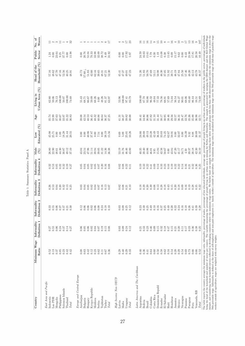
all countries considered, the ratio of the minimum wage and the 70th wage percentile is at 0.49,
as can be seen in Table 1. We can also infer from the data that the generosity of the minimum
wage has increased in recent decades, as indicated by the crossplot in Figure 3, displaying on
the y axis the ratio in the 1990s and on the x axis the ratio in the 2000s.
FIGURE 3 AROUND HERE
Such high figures in the effectiveness of the minimum wage may be not as harmful on formal
employment as expected in the presence of non-compliance. As expected, non-compliance with
the minimum wage law in developing labor markets is high, and increasing with the level of
the minimum wage, as illustrated in Figure 5. What is true at the national level is also true
for each labor market group, as shown in Figures A.1 and A.2. There does not seem to be a
difference across groups, indicating that our identification does not suffer from heterogeneity
in compliance across groups.
FIGURES 5 AROUND HERE
In some cases, more than 50 percent of the workers’ wages are below the minimum wage.
The pervasiveness of non-compliance with the law suggests that the impact of the minimum
wage on formality may be less obvious than the high levels of effectiveness of the minimum
wage may suggest, and potentially non-linear. If the minimum wage is very low, firms may not
need to resort to informal employment. If instead the minimum wage is too high, firms may
prefer risking fines by paying a wage below the legislated minimum. Thus, firms are likely to
trade off two forms of informality in developing labor markets: wage employment below the
minimum wage and self-employment.
The minimum wage has a different level of effectiveness depending on the group of workers we
consider, as it is clearly indicated by the difference between the strictness of the minimum wage
for specific groups and the country averages. Panel (a) in Figure 5 shows a kernel of the relative
10
effectiveness of the minimum wage across age groups, after pooling the data across countries
and years. As expected, young workers (18-29) are the most affected by the minimum wage
legislation: the minimum wage for them is more binding than the average. The least affected by
the minimum wage are instead the prime age workers (30-50). In panel (b) we also find that the
minimum wage is generally more binding for less educated workers. Differences across gender
are less pronounced, in part because female wages are more compressed than males (panel (c)).
Our identification strategy exploits this heterogeneity in the minimum wage’s strictness across
labor market groups.
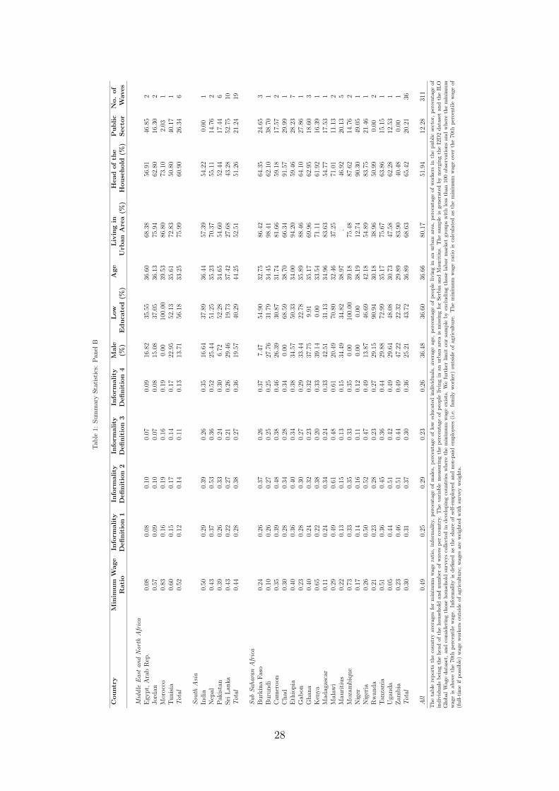
Table 1 also presents the average informality rate (among the economically active) in each
country of our sample, according to different definitions. Our baseline definition of informality
includes all the workers outside of agriculture who are either self-employed or family-workers,
to whom the minimum wage does not apply (definition 2). As a robustness check we will also
adopt other definitions of informality: self-employed outside of agriculture only (definition 1);
low educated (primary education or no schooling) self-employed outside of agriculture only
(definition 3); low educated (primary education or no schooling) self-employed and unpaid
family employees outside of agriculture (definition 4). In the table we also show the average
percentage of male workers in our sample by country, the percentage of low educated workers,
their average age, the percentage of people living in urban areas, the percentage of workers who
are the head of the household and the number of waves available per country.
4 Empirical Findings
4.1 Baseline Specification
Table 6 presents our baseline empirical findings. The results are presented by column
augmenting the model with additional controls, starting with country fixed effects only in
column (2), adding year fixed effects in column (3), their interaction in column (4), additional
individual-level controls in column (5), and an interaction between country fixed effects and
individual-level controls in column (6). The individual-level controls include a dummy signalling
if the individual has a low level of education (primary education or no schooling), a dummy
11
for individuals who are 18-29 years old, a dummy for individuals who are 30-50 years old, a
dummy for being a female, an indicator of whether the individual resides in an urban versus a
rural area, industry (mining, manufacturing, public utilities, construction, retail and wholesale
trade, transport and communications, financial and business services, public administration or
other unspecified services), whether the individual is the head of the household/spouse/other
relative, and the household size.
TABLE 6 AROUND HERE
Our results are consistent across columns, with some differences in the point estimates. A
higher minimum wage is typically associated with a larger share of informality and the effect is
statistically significant at the 1 percent level. According to our preferred specification in column
(6), a 1 percentage point increase in the ratio of the minimum wage over the 70th percentile
of wages outside agriculture, increases the probability to be self-employed by 0.204 percentage
points. Given that the standard deviation of the minimum wage ratio in the estimation sample
is 0.239 and that the average informality share is 0.290, one standard deviation increase in the
minimum wage ratio increases informality by 16.81 percent. The estimated effect is significant
at the 1 percent level.7
Our baseline specification imposes linearity in the effect of the minimum wage ratio on self-
employment. However, the stringency of the minimum wage may have a non-linear impact on
informality. In Table 5 we test whether the effect of minimum wage legislation on informality
is non-linear. In order to do that, we identify in every country/year the groups for which
the minimum wage lies within the 1st, 2nd, 3rd, 4th, 5th, 6th and 7th deciles of the wage
distribution. We then replace in the regressions the minimum wage ratio with a set of indicator
variables for each of the minimum wage deciles. Our results show that the impact of the
minimum wage on informality increases almost monotonically with the decile of the minimum
wage. If the minimum wage lies in the 7th decile of the cell’s wage distribution, the probability
to be self-employed is 0.108 percentage points larger than if the minimum wage lies in the first
decile of the wage distribution.
7A standard deviation of the minimum wage ratio in the estimation sample of 0.239 is pretty large (thesample average is 0.487).
12
TABLE 5 AROUND HERE
We find no evidence of the impact of the minimum wage on informality levelling out as the
minimum wage level approaches or even crosses the median. On the contrary, we find that
moving the minimum wage from the 5th to the 7th decile of the distribution of wages still
presents a large step jump in informal employment, with a difference of 0.029 percentage points
that is statistically significant at the 1% level.
4.2 Heterogeneity Across Countries
Most observations in our sample come from surveys collected in 17 Latin American coun-
tries.8 In columns (1)-(4) of Table 7 we check whether our estimated effect is heterogeneous
across geographical areas, by examining separately the effects in and outside Latin America
and the effects in higher and lower-income countries. We notice that a rise in the minimum
wage increases the probability to be self-employed worldwide and that the effect is stronger in
Latin America and in lower income countries.
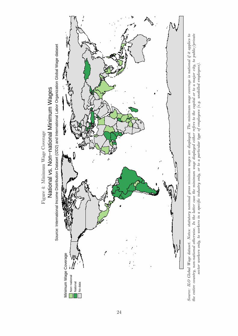
In column (5) we only consider countries where the minimum wage legislation is applied
uniformly to the whole nation rather than countries where it is an institution pertaining to
specific sub-national groups, like workers in specific geographical areas, sectors, public versus
private jobs, low skilled workers or a combination of all elements above.9 The world distribution
of national versus non-national minimum wage provision is displayed in Figure 4.
We find that, independently of the type of minimum wage legislation, a more binding
minimum wage increases the share of self-employed, more so in countries where the minimum
wage is non-national.
In column (6) we estimate our model after including workers from the private sector that
in general may be characterized by a smaller share of minimum wage employees and where
wage setting is typically managed differently from the public sector. The point estimate is
8They represent 184 out of the total 311 survey waves, i.e. 55.7% of the total observations.9If there are multiple sub-national minimum wages, we consider the sub-national minimum wage available
in the ILO dataset.
13
smaller in magnitude when the public sector is only in included (column (7)), but they are not
significantly different from each other.
Furthermore, we check whether the effect is stronger in countries where the rule of law
is more binding. In columns (8)-(9) such binary classification is time invariant, since the
countries are grouped according to weather they are more frequently classified above or below
the median.10
Our estimates point to a marginally larger point estimate for countries where the rule of
law is above the median, as expected.
TABLE 7 AROUND HERE
We also check whether the non-linearity in the minimum wage effects presented in Table 5,
are also present in the sub-samples considered above. Our findings, presented in Table A1 in the
Appendix, suggest that the effects across labor market groups increase almost monotonically
in each subsample.
5 Robustness Checks
We perform a series of robustness checks that are displayed in Table 8. Let us recall that
since the minimum wage legislation usually applies to full-time workers only, the minimum wage
ratio is calculated using the wage of full-time workers when it is possible to distinguish between
full and part-time workers in the data. However, in some cases it is not possible to make that
distinction, and the ratio is based on the wages of both full and part-time workers 11. Hence, as
a robustness check, we limit the sample to those survey waves where it is possible to distinguish
1022 countries in the sample switch across years from having rule of law values below the median to valuesabove the median (or vice versa); 20 countries have values always above; 12 countries have values always below;5 countries only have waves with missing values so they are neither above nor below. We divide countries intotwo groups: in the first group there are the 10 countries that more frequently have rule of law values above themedian together with countries that always have values above the median and in the second group there arethe 12 countries that more frequently have values below the rule of law together with countries that have ruleof law below the median. The 3 countries that never have values for the Rule of Law are excluded from theestimations.
11It is not possible to make a distinction between full and part-time workers when hours worked are notrecorded in the survey or when the variable has too many missing values
14
between full and part-time workers. In order to do this we discard those waves where the hours
of work are missing for more than 20% of the working population, or where the distribution of
weekly hours does not exceed 35, implying that the variable is measured with error. When we
proceed this way we are left with 50 countries, 375 country groups and 8,828,249 observations.
The model in column (1) presents our findings when the sample includes only those surveys
in which we can identify and exclude part-time workers, so that the minimum wage ratio is
computed more precisely. The point estimates are very close to the estimates on the full sample.
TABLE 8 AROUND HERE
As a further robustness check, we estimate our model restricting the sample to cells whose
dimension consists of at least 200 observations. This choice limits the possibility that our
measure of the minimum wage ratio is corrupted by measurement error due to a small cell size.
We face a trade-off between the more accurate measures obtained by the larger cell size and the
possible bias introduced by the selection of those cells that are large enough. Our sample is now
slightly smaller, since we lose around two percent of the observations. The estimates presented
in column (2) show that our results are mostly unaffected, indicating that we are unlikely to
suffer from sampling error. Robustness checks with larger cell sizes have been performed with
similar results and are available upon request.
In columns (6)-(7) of Table 7 we included workers from either the public or private sector
only. However, the information on the occupational sector (public vs. private) in some surveys
has a large number of missing values. As a further robustness check we then exclude from our
sample those survey waves where the percentage of missing values in the variable indicating the
sector of occupation is higher than 10 percent, i.e. those surveys where we are forced to select
a share of the respondents that is smaller than 90 percent. In columns (3)-(4) (Table 8) we
show that the estimates for workers in the private sector when we exclude survey waves with
more than 10% missing values are unaffected, but for the public sector they lose significance.
Moreover, we check whether our results are robust to different definitions of informality.
In the paper we defined having an informal job outside of agriculture as being self-employed
or a family worker, i.e. belonging to the pool of workers who by definition are not covered
15
by minimum wage legislation. In column (5) of the Table, informal workers are defined as the
share of self-employed in total employment outside agriculture, i.e. family workers are excluded
from the definition; in column (6) informal workers are defined as the share of low educated
(primary education or no schooling) self-employed only in total employment outside agriculture;
in column (7) informality is defined as the share of low educated (primary education or no
schooling) self-employed and unpaid family employees in total employment outside agriculture.
Results vary somewhat in magnitude across definitions, but irrespectively of the definition
adopted, the lesson from our findings is unchanged.
We also check whether our results hold when we change the definition of the effectiveness
of the minimum wage. In the baseline specifications we defined it as the ratio of the minimum
wage over the 70th percentile wage of wage workers outside of agriculture. In columns (8) and
(9) we change the definition and use, respectively, the 65th and the 75th percentile wage for
constructing the minimum wage ratio. Our results do not vary much after this modification.
Finally, we check whether our results hold when instead of giving equal weight to each cell
(i.e. each country/group/year), we give equal weight to each wave (i.e. each country/year). In
this way we avoid giving greater importance to waves that have more cells in our sample. Our
results hold after this modification.
6 Conclusions
We presented a set of new empirical findings on the economic implications of minimum wage
legislation in developing countries obtained from a unique newly assembled dataset containing
311 micro surveys from 59 developing countries during the years 1995-2012. The focus of
our analysis is on the relationship between minimum wages and informality, measured as the
probability of being self-employed or a family worker. We avoid common pitfalls of cross-
country comparisons by relying on the effectiveness of the minimum wage across labor market
groups for identification. Our identification strategy exploits the relative bite of the minimum
wage across age, gender and education groups within country years.
Our estimates show that a more generous minimum wage is typically associated with a
16
larger share of informality. Our preferred baseline effect indicates that a 1 percentage point
increase in the ratio of the minimum wage over the 70th percentile of wages outside agriculture
in a specific cell, increases the self-employment share of that specific cell by 0.204 percentage
points. The effect corresponds to a one standard deviation increase in the ratio of the minimum
wage over the 70th percentile of formal wages, equal to 0.239 in our sample, being associated
with an increase in the self-employment share of that specific cell by 16.81 percent. The effect
is highly significant and very robust across a large number of alternative specifications.
We find that the impact of the minimum wage on informality increases almost monotonically
with the generosity of the minimum wage. More specifically, if the minimum wage lies in the
7th decile of the cell’s wage distribution, the estimated probability to be self-employed is 0.108
percentage points larger than if the minimum wage lies in the first decile of the wage distribution.
Our results show that, on average, the minimum wage is likely to have relatively important
effects on informality in the developing world, a feature that should be borne in mind when
evaluating the welfare consequences of reforming minimum wage legislation. Governments
aiming to reduce poverty using the minimum wage as a policy lever should take into account
that the effects on informality are likely to be concentrated precisely across those groups that
are more vulnerable to poverty, in particular the young and the less educated. The estimation
of such effects is of great relevance for the policy maker willing to trade a certain increase
in informality for a welfare benefit associated to higher wages. Further research is needed
to evaluate the general equilibrium effect of minimum wage policies in developing countries,
considering the implications of such policies in terms of general employment levels.
17
References
Addison, John T., & Ozturk, Orgul Demet. 2012. Minimum Wages, Labor Market Institutions,
and Female Employment and Unemployment: A Cross-Country Analysis. Industrial and
Labor Relations Review, 65(4), 779–809. 1
Addison, John T., Blackburn, McKinley L., & Cotti, Chad D. 2013. Minimum wage increases
in a recessionary environment. Labour Economics, 23(C), 30–39. 1
Bell, Linda A. 1997. The Impact of Minimum Wages in Mexico and Colombia. Journal of
Labor Economics, 15(3), S102–35. 1
Bosch, Mariano, & Maloney, William F. 2010. Comparative analysis of labor market dynamics
using Markov processes: An application to informality. Labour Economics, 17(4), 621 – 631.
1
Brown, Alessio, Merkl, Christian, & Snower, Dennis J. 2014. The minimum wage from a
two-sided perspective. Economics Letters, 124(3), 389–391. 1
Card, David. 1992. Using Regional Variation in Wages to Measure the Effects of the Federal
Minimum Wage. Industrial & Labor Relations Review, 46(1), 22–37. 1
Colin Cameron, A., & Miller, Douglas L. 2015. A Practitioner?s Guide to Cluster-Robust
Inference. Journal of Human Resources, 50(2), 317–372. 2
Del Carpio, Ximena, Messina, Julin, & Sanz-de Galdeano, Anna. 2014 (Jan.). Minimum Wage:
Does It Improve Welfare in Thailand? IZA Discussion Papers 7911. Institute for the Study
of Labor (IZA). 1
Dickens, Richard, Machin, Stephen, & Manning, Alan. 1999. The Effects of Minimum Wages
on Employment: Theory and Evidence from Britain. Journal of Labor Economics, 17(1),
1–22. 1
Draca, Mirko, Machin, Stephen, & Reenen, John Van. 2011. Minimum Wages and Firm Prof-
itability. American Economic Journal: Applied Economics, 3(1), 129–51. 1
18
Dube, Arindrajit, Lester, T. William, & Reich, Michael. 2010. Minimum Wage Effects Across
State Borders: Estimates Using Contiguous Counties. The Review of Economics and Statis-
tics, 92(4), 945–964. 1
Gindling, T.H., & Terrell, Katherine. 2007. The effects of multiple minimum wages throughout
the labor market: The case of Costa Rica. Labour Economics, 14(3), 485–511. 1
Gindling, T.H., & Terrell, Katherine. 2009. Minimum wages, wages and employment in various
sectors in Honduras. Labour Economics, 16(3), 291–303. 1
International Labour Office (ILO). 2013. ILOSTAT Database. 3
Lee, David S. 1999. Wage inequality in the United States during the 1980s: rising dispersion
or falling minimum wage? The Quarterly Journal of Economics, 114(3), 977–1023. 1, 2
Lemos, Sara. 2009. Minimum wage effects in a developing country. Labour Economics, 16(2),
224–237. 1
Maloney, William. 1999. Does Informality Imply Segmentation in Urban Labor Markets? Evi-
dence from Sectoral Transitions in Mexico. World Bank Economic Review, 13(2), 275–302.
1
Maloney, William F., Nunez, Jairo, Cunningham, Wendy, Fiess, Norbert, Montenegro, Claudio,
Murrugarra, Edmundo, Santamaria, Mauricio, & Sepulveda, Claudia. 2001 (Apr.). Measuring
the impact of minimum wages : evidence from Latin America. Policy Research Working Paper
Series 2597. The World Bank. 1
Neumark, David, & Wascher, William. 1992. Employment effects of minimum and subminimum
wages: Panel data on state minimum wage laws. Industrial and Labor Relations Review,
46(1), 55–81. 1
Neumark, David, Salas, J. M. Ian, & Wascher, William. 2014. Revisiting the Minimum
Wage?Employment Debate: Throwing Out the Baby with the Bathwater? Industrial &
Labor Relations Review, 67(3 suppl), 608–648. 1
19
Nguyen Viet, Cuong. 2010 (Dec.). The Impact of a Minimum Wage Increase on Employment,
Wages and Expenditures of Low-Wage Workers in Vietnam. MPRA Paper 36751. University
Library of Munich, Germany. 1
Nunziata, Luca. 2015. Immigration and Crime: Evidence From Victimization Data. Journal
of Population Economics, 28(3). 2
Rajan, Raghuram G, & Zingales, Luigi. 1998. Financial Dependence and Growth. American
Economic Review, 88(3), 559–86. 1, 2
Verbeek, M., & Nijman, T. 1992. Can cohort data be treated as genuine panel data? Empirical
Economics, 17(1), 9–23. 2
Verbeek, Marno, & Nijman, Theo. 1993. Minimum {MSE} estimation of a regression model
with fixed effects from a series of cross-sections. Journal of Econometrics, 59(1-2), 125 – 136.
2
World Bank. 2013. International Income Distribution Database (I2D2). 3
20
Fig
ure
1:M
inim
um
Wag
eR
atio
Acr
oss
Cou
ntr
ies
0− 0.1−
0.2−
0.3−
0.4−
0.5−
0.6−
0.7−
0.8−
No
data
MW
/70t
h W
age
Per
cent
ile R
atioS
ourc
e: In
tern
atio
nal I
ncom
e D
istr
ibut
ion
Dat
aset
(I2
D2)
and
Inte
rnat
iona
l Lab
or O
rgan
izat
ion
Glo
bal W
age
data
set
Ave
rage
Min
imum
Wag
e R
atio
Acr
oss
Cou
ntrie
s
Note
s:T
he
wage
rati
osh
ow
nin
the
map
isa
wei
ghte
dave
rage
of
the
min
imu
mw
age
/70th
perc
enti
lew
age
inth
eco
un
try
acr
oss
cell
s(w
her
eth
ew
eigh
tsare
the
share
sof
each
cell
wage
emplo
ymen
tin
tota
lw
age
emplo
ymen
t).
Ifth
ere
are
more
surv
eyw
ave
sfo
ra
cou
ntr
y,w
eta
kea
sim
ple
ave
rage
of
the
cou
ntr
yave
rage
sacr
oss
years
.T
he
sam
ple
com
esfr
om
mer
gin
gth
eI2
D2
data
set
an
dth
eIL
OG
loba
lW
age
data
set.
We
keep
hou
sehold
surv
eys
of
dev
elopin
gco
un
trie
sw
her
eth
em
inim
um
wage
exis
ts;
we
furt
her
lim
itou
rsa
mple
tola
bor
mark
etgr
ou
ps
(cel
ls)
form
edby
more
than
100
obs
erva
tion
san
dw
her
eth
em
inim
um
wage
isbe
low
the
med
ian
wage
.Y
ears
1995-2
012.
21
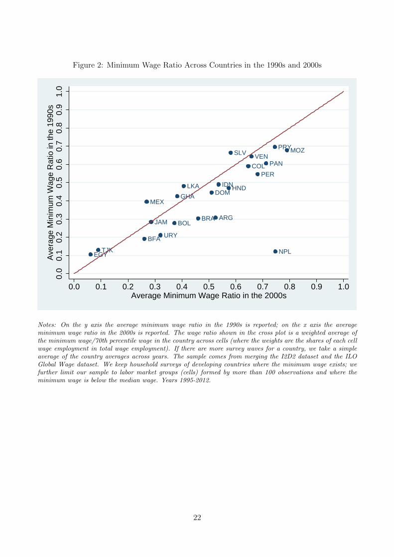
Figure 2: Minimum Wage Ratio Across Countries in the 1990s and 2000s
ARG
BFA
BOLBRA
COL
DOM
EGY
GHAHNDIDN
JAM
LKA
MEX
MOZ
NPL
PAN
PER
PRYSLV
TJK
URY
VEN
0.0
0.1
0.2
0.3
0.4
0.5
0.6
0.7
0.8
0.9
1.0
Ave
rage
Min
imum
Wag
e R
atio
in th
e 19
90s
0.0 0.1 0.2 0.3 0.4 0.5 0.6 0.7 0.8 0.9 1.0Average Minimum Wage Ratio in the 2000s
Notes: On the y axis the average minimum wage ratio in the 1990s is reported; on the x axis the averageminimum wage ratio in the 2000s is reported. The wage ratio shown in the cross plot is a weighted average ofthe minimum wage/70th percentile wage in the country across cells (where the weights are the shares of each cellwage employment in total wage employment). If there are more survey waves for a country, we take a simpleaverage of the country averages across years. The sample comes from merging the I2D2 dataset and the ILOGlobal Wage dataset. We keep household surveys of developing countries where the minimum wage exists; wefurther limit our sample to labor market groups (cells) formed by more than 100 observations and where theminimum wage is below the median wage. Years 1995-2012.
22
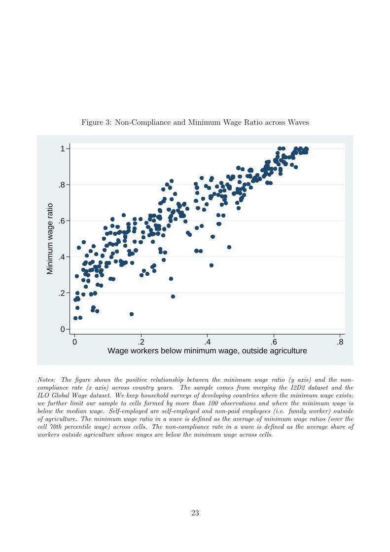
Figure 3: Non-Compliance and Minimum Wage Ratio across Waves
0
.2
.4
.6
.8
1
Min
imum
wag
e ra
tio
0 .2 .4 .6 .8Wage workers below minimum wage, outside agriculture
Notes: The figure shows the positive relationship between the minimum wage ratio (y axis) and the non-compliance rate (x axis) across country years. The sample comes from merging the I2D2 dataset and theILO Global Wage dataset. We keep household surveys of developing countries where the minimum wage exists;we further limit our sample to cells formed by more than 100 observations and where the minimum wage isbelow the median wage. Self-employed are self-employed and non-paid employees (i.e. family worker) outsideof agriculture. The minimum wage ratio in a wave is defined as the average of minimum wage ratios (over thecell 70th percentile wage) across cells. The non-compliance rate in a wave is defined as the average share ofworkers outside agriculture whose wages are below the minimum wage across cells.
23
Fig
ure
4:M
inim
um
Wag
eC
over
age
Non
−na
tiona
l
Nat
iona
l
No
data
Min
imum
Wag
e C
over
age
Sou
rce:
Inte
rnat
iona
l Inc
ome
Dis
trib
utio
n D
atas
et (
I2D
2) a
nd In
tern
atio
nal L
abor
Org
aniz
atio
n G
loba
l Wag
e da
tase
t
Nat
iona
l vs.
Non
−na
tiona
l Min
imum
Wag
es
Sou
rce:
ILO
Glo
bal
Wage
data
set.
Note
s:st
atu
tory
nom
inal
gross
min
imu
mw
age
sare
dis
pla
yed.
The
min
imu
mw
age
cove
rage
isn
ati
on
al
ifit
appli
esto
the
enti
reco
un
try,
non
-nati
on
al
oth
erw
ise.
Inth
ela
tter
case
the
min
imu
mw
age
dis
pla
yed
eith
erre
fers
toth
eca
pit
al
or
toa
majo
rci
ty,
topu
blic
/pri
vate
sect
or
work
ers
on
ly,
tow
ork
ers
ina
spec
ific
indu
stry
on
ly,
or
toa
part
icu
lar
type
of
emplo
yees
(e.g
.u
nsk
ille
dem
plo
yees
).
24
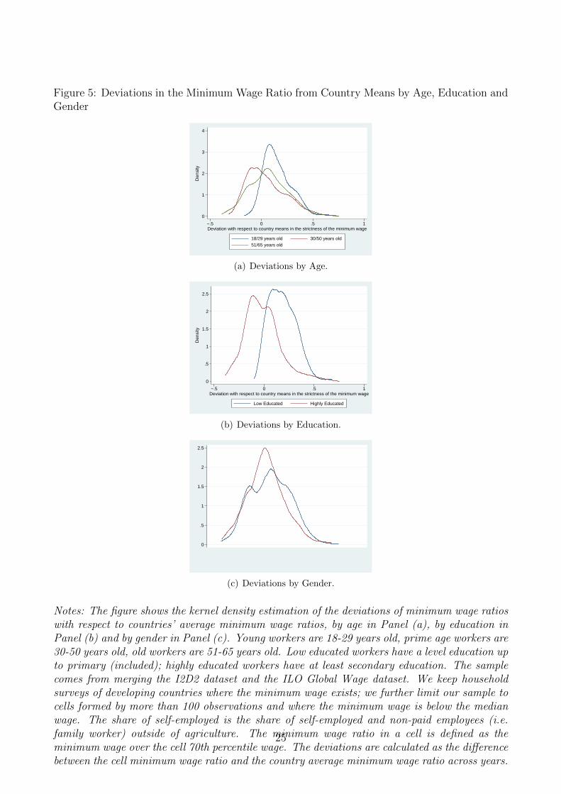
Figure 5: Deviations in the Minimum Wage Ratio from Country Means by Age, Education andGender
0
1
2
3
4
Den
sity
−.5 0 .5 1Deviation with respect to country means in the strictness of the minimum wage
18/29 years old 30/50 years old51/65 years old
(a) Deviations by Age.
0
.5
1
1.5
2
2.5
Den
sity
−.5 0 .5 1Deviation with respect to country means in the strictness of the minimum wage
Low Educated Highly Educated
(b) Deviations by Education.
0
.5
1
1.5
2
2.5
(c) Deviations by Gender.
Notes: The figure shows the kernel density estimation of the deviations of minimum wage ratioswith respect to countries’ average minimum wage ratios, by age in Panel (a), by education inPanel (b) and by gender in Panel (c). Young workers are 18-29 years old, prime age workers are30-50 years old, old workers are 51-65 years old. Low educated workers have a level education upto primary (included); highly educated workers have at least secondary education. The samplecomes from merging the I2D2 dataset and the ILO Global Wage dataset. We keep householdsurveys of developing countries where the minimum wage exists; we further limit our sample tocells formed by more than 100 observations and where the minimum wage is below the medianwage. The share of self-employed is the share of self-employed and non-paid employees (i.e.family worker) outside of agriculture. The minimum wage ratio in a cell is defined as theminimum wage over the cell 70th percentile wage. The deviations are calculated as the differencebetween the cell minimum wage ratio and the country average minimum wage ratio across years.
25

26
Tab
le1:
Sum
mar
ySta
tist
ics:
Pan
elA
Countr
yM
inim
um
Wage
Info
rmality
Info
rmality
Info
rmality
Info
rmality
Male
Low
Age
Liv
ing
inH
ead
of
the
Public
No.
of
Rati
oD
efinit
ion
1D
efinit
ion
2D
efinit
ion
3D
efinit
ion
4(%
)E
duca
ted
(%)
Urb
an
Are
a(%
)H
ouse
hold
(%)
Sect
or
Waves
Eas
tA
sia
and
Pac
ific
Indon
esia
0.52
0.27
0.33
0.26
0.32
26.8
045
.98
35.7
462
.80
57.1
61.
2411
Lao
PD
R0.
130.
550.
550.
530.
5322
.90
25.7
133
.99
59.0
648
.62
0.00
2M
ongo
lia
0.37
0.06
0.06
0.04
0.05
48.6
10.
0037
.63
76.1
347
.70
23.6
43
Philip
pin
es0.
850.
240.
270.
200.
2244
.30
1.89
38.6
710
0.00
47.1
69.
2511
Sol
omon
Isla
nds
0.23
0.37
0.37
0.32
0.32
30.8
718
.28
33.0
750
.07
52.5
637
.77
1T
hai
land
0.42
0.14
0.21
0.13
0.19
49.1
231
.44
35.2
210
0.00
40.2
50.
004
Tot
al0.
420.
270.
300.
250.
2737
.10
20.5
536
.83
74.6
848
.91
11.9
832
Eu
rope
and
Cen
tral
Eu
rope
Aze
rbai
jan
0.08
0.06
0.12
0.03
0.05
43.8
40.
0039
.08
55.4
348
.73
0.00
1B
ulg
aria
0.63
0.05
0.06
0.04
0.04
23.5
40.
0042
.54
68.7
157
.60
¿20
.76
4H
unga
ry0.
420.
060.
060.
050.
0547
.96
40.8
640
.53
66.6
751
.83
51.0
41
Kyrg
yz
Rep
ublic
0.12
0.02
0.02
0.02
0.02
51.1
437
.87
36.4
559
.09
42.6
070
.33
1M
oldov
a0.
230.
040.
060.
040.
0539
.94
0.00
40.3
268
.26
62.4
433
.98
1Ser
bia
0.62
0.07
0.08
0.07
0.07
39.0
57.
5440
.88
0.00
39.6
532
.09
1T
aji
kis
tan
0.11
0.19
0.24
0.16
0.20
31.2
20.
0036
.64
48.2
648
.31
38.7
22
Turk
ey0.
670.
150.
180.
130.
1614
.36
38.1
936
.37
81.3
767
.21
8.49
6T
otal
0.36
0.08
0.10
0.07
0.08
36.3
815
.56
37.2
563
.97
52.3
031
.92
17
Hig
hIn
com
eN
onO
EC
DL
atvia
0.29
0.03
0.03
0.02
0.02
53.1
90.
6941
.31
53.9
645
.41
0.00
4M
alta
0.40
0.09
0.09
0.08
0.08
31.7
65.
0938
.27
100.
0047
.27
0.00
2U
rugu
ay0.
290.
240.
250.
210.
2246
.46
25.0
139
.82
97.4
149
.01
17.9
217
Tot
al0.
330.
120.
120.
100.
1143
.80
10.2
630
.00
83.7
947
.23
5.97
23
Lat
inA
mer
ica
and
The
Car
ibbe
anA
rgen
tina
0.46
0.21
0.23
0.18
0.19
40.3
524
.66
38.4
110
0.00
51.2
624
.59
16B
oliv
ia0.
360.
330.
390.
290.
3339
.40
29.8
834
.80
87.7
051
.93
16.0
311
Bra
zil
0.41
0.23
0.25
0.20
0.22
44.0
649
.13
36.0
693
.86
50.7
015
.61
16C
olom
bia
0.64
0.46
0.49
0.39
0.41
46.0
123
.28
37.8
296
.32
47.6
97.
7914
Cos
taR
ica
0.60
0.09
0.10
0.08
0.09
9.95
42.4
931
.10
48.0
453
.11
0.30
9D
omin
ican
Rep
ubl
0.50
0.15
0.16
0.13
0.14
15.9
436
.43
31.4
477
.33
50.9
81.
1915
Ecu
ador
0.58
0.32
0.37
0.28
0.33
42.5
633
.03
38.1
778
.56
46.3
015
.08
10E
lSal
vador
0.62
0.18
0.25
0.18
0.23
50.6
774
.25
30.9
568
.91
37.0
50.
388
Hai
ti0.
340.
470.
480.
430.
440.
0062
.67
38.4
657
.69
51.9
211
.65
1H
ondura
s0.
540.
150.
200.
150.
1943
.84
59.9
129
.56
74.0
439
.71
0.09
16Jam
aica
0.28
0.21
0.22
0.20
0.22
47.2
00.
0032
.57
56.5
446
.19
15.1
74
Mex
ico
0.29
0.20
0.24
0.18
0.22
41.1
732
.07
36.3
184
.27
47.8
49.
6210
Nic
arag
ua
0.54
0.11
0.16
0.09
0.14
34.7
10.
0028
.47
90.0
125
.50
0.00
2P
anam
a0.
690.
170.
180.
160.
164.
5016
.39
33.7
668
.06
57.4
60.
4317
Par
aguay
0.73
0.23
0.26
0.19
0.21
39.3
79.
3235
.26
83.4
048
.20
21.9
813
Per
u0.
660.
360.
410.
280.
3238
.18
8.88
35.8
886
.44
42.1
317
.81
16V
enez
uel
a,R
B0.
660.
380.
390.
350.
3642
.30
30.8
936
.98
18.5
143
.78
20.5
89
Tot
al0.
520.
250.
280.
220.
2534
.10
31.3
732
.71
74.6
946
.57
10.4
918
7
Th
eta
ble
rep
orts
the
cou
ntr
yav
erag
esfo
rm
inim
um
wag
era
tio,
info
rmal
ity,
per
centa
geof
mal
es,
per
centa
geof
low
edu
cate
din
div
idu
als,
aver
age
age,
per
centa
geof
peo
ple
livin
gin
anu
rban
area
,p
erce
nta
geof
wor
kers
inth
epu
bli
cse
ctor
,p
erce
nta
ge
of
ind
ivid
uals
bei
ng
the
hea
dof
the
hou
seh
old
and
nu
mb
erof
wav
esp
erco
untr
y.T
he
vari
able
mea
suri
ng
the
per
centa
geof
peo
ple
livin
gin
anu
rban
area
ism
issi
ng
for
Ser
bia
and
Mau
riti
us.
Th
esa
mp
leis
gen
erat
edby
mer
gin
gth
eI2
D2
dat
aset
and
the
ILO
Glo
bal
Wage
dat
aset
,an
dco
nsi
der
ing
thos
eh
ouse
hol
dsu
rvey
sco
llec
ted
ind
evel
opin
gco
untr
ies
wh
ere
the
min
imu
mw
age
exis
ts.
We
furt
her
lim
itou
rsa
mp
leby
excl
ud
ing
thos
ela
bor
mar
ket
grou
ps
wit
hle
ssth
an10
0ob
serv
atio
ns
and
wh
ere
the
min
imu
mw
age
isab
ove
the
70th
per
centi
lew
age.
Info
rmal
ity
isd
efin
edas
the
shar
eof
self
-em
plo
yed
and
non
-pai
dem
plo
yees
(i.e
.fa
mil
yw
ork
er)
outs
ide
ofag
ricu
ltu
re.
Th
em
inim
um
wag
era
tio
isca
lcu
late
das
the
min
imu
mw
age
over
the
70th
per
centi
lew
age
of(f
ull-t
ime
ifp
oss
ible
)w
age
wor
kers
outs
ide
ofag
ricu
ltu
re;
wag
esar
ew
eigh
ted
wit
hsu
rvey
wei
ghts
.
27
Tab
le1:
Sum
mar
ySta
tist
ics:
Pan
elB
Cou
ntr
yM
inim
um
Wage
Info
rmali
tyIn
form
ali
tyIn
form
ali
tyIn
form
ali
tyM
ale
Low
Age
Liv
ing
inH
ead
of
the
Pu
bli
cN
o.
of
Rati
oD
efi
nit
ion
1D
efi
nit
ion
2D
efi
nit
ion
3D
efi
nit
ion
4(%
)E
du
cate
d(%
)U
rban
Are
a(%
)H
ou
seh
old
(%)
Sect
or
Waves
Mid
dle
Eas
tan
dN
orth
Afr
ica
Egy
pt,
Ara
bR
ep.
0.08
0.08
0.10
0.07
0.09
16.8
235
.55
36.6
068
.38
56.9
146
.85
2Jor
dan
0.57
0.09
0.10
0.07
0.08
15.0
837
.05
36.1
375
.94
62.8
016
.30
2M
orocc
o0.
830.
160.
190.
160.
190.
0010
0.00
39.5
386
.80
73.1
02.
031
Tunis
ia0.
600.
150.
170.
140.
1722
.95
52.1
335
.61
72.8
350
.80
40.1
71
Tot
al0.
520.
120.
140.
110.
1313
.71
56.1
833
.25
75.9
960
.90
26.3
46
Sou
thA
sia
India
0.50
0.29
0.39
0.26
0.35
16.6
437
.89
36.4
457
.39
54.2
20.
001
Nep
al0.
430.
370.
530.
360.
5225
.44
51.2
535
.23
70.3
755
.11
14.7
62
Pak
ista
n0.
390.
260.
330.
240.
306.
7252
.28
34.6
554
.60
52.4
417
.44
6Sri
Lan
ka0.
430.
220.
270.
210.
2629
.46
19.7
337
.42
27.6
843
.28
52.7
510
Tot
al0.
440.
280.
380.
270.
3619
.57
40.2
944
.25
52.5
151
.26
21.2
419
Su
bS
ahar
anA
fric
aB
urk
ina
Fas
o0.
240.
260.
370.
260.
377.
4754
.90
32.7
586
.42
64.3
524
.65
3B
uru
ndi
0.10
0.26
0.27
0.25
0.25
27.7
631
.79
34.4
598
.41
62.1
038
.70
1C
amer
oon
0.35
0.39
0.48
0.38
0.46
26.3
930
.87
31.7
481
.66
59.1
817
.57
2C
had
0.30
0.28
0.34
0.28
0.34
0.00
68.5
938
.70
66.3
491
.57
29.9
91
Eth
iopia
0.40
0.36
0.40
0.34
0.38
34.5
750
.33
34.0
094
.20
59.4
628
.23
7G
abon
0.23
0.28
0.30
0.27
0.29
33.4
422
.78
35.8
988
.46
64.1
027
.86
1G
han
a0.
400.
240.
320.
230.
3237
.75
9.91
35.1
769
.96
62.9
518
.60
3K
enya
0.65
0.22
0.38
0.20
0.33
39.1
40.
0033
.54
71.1
161
.92
16.3
91
Mad
agas
car
0.11
0.24
0.34
0.24
0.33
42.5
131
.13
34.9
683
.63
54.7
717
.53
1M
alaw
i0.
290.
490.
610.
480.
6120
.49
70.8
032
.46
37.2
571
.01
11.1
32
Mau
riti
us
0.22
0.13
0.15
0.13
0.15
34.4
934
.82
38.9
7.
46.9
220
.13
5M
ozam
biq
ue
0.73
0.33
0.35
0.33
0.35
0.00
100.
0039
.18
75.4
887
.62
14.7
62
Nig
er0.
170.
140.
160.
110.
120.
000.
0038
.19
12.7
490
.30
49.0
51
Nig
eria
0.26
0.50
0.52
0.47
0.49
13.8
746
.69
42.1
854
.89
83.7
521
.46
1R
wan
da
0.21
0.23
0.28
0.23
0.27
29.1
590
.94
30.1
838
.96
50.9
90.
002
Tan
zania
0.51
0.36
0.45
0.36
0.44
29.8
872
.99
35.1
775
.67
63.8
615
.15
1U
ganda
0.05
0.44
0.51
0.42
0.49
29.6
448
.08
30.7
347
.58
62.2
812
.53
1Z
ambia
0.23
0.46
0.51
0.44
0.49
47.2
222
.32
29.8
983
.90
40.4
80.
001
Tot
al0.
300.
310.
370.
300.
3625
.21
43.7
236
.89
68.6
365
.42
20.2
136
All
0.49
0.25
0.29
0.23
0.26
36.4
836
.60
36.6
680
.17
51.9
412
.28
311
The
table
rep
orts
the
countr
yav
erag
esfo
rm
inim
um
wag
era
tio,
info
rmality
,p
erce
nta
geof
male
s,p
erce
nta
geof
low
educa
ted
indiv
iduals
,av
erag
eag
e,p
erce
nta
geof
peo
ple
livin
gin
an
urb
anar
ea,
per
centa
geof
wor
kers
inth
epublic
sect
or,
per
centa
ge
ofin
div
idual
sb
eing
the
hea
dof
the
hou
sehol
dan
dnum
ber
of
wav
esp
erco
untr
y.T
he
vari
able
mea
suri
ng
the
per
centa
geof
peo
ple
livin
gin
an
urb
an
are
ais
mis
sing
for
Ser
bia
and
Mauri
tius.
The
sam
ple
isge
ner
ated
by
mer
ging
the
I2D
2data
set
and
the
ILO
Glo
bal
Wag
edata
set,
and
consi
der
ing
those
hou
sehold
surv
eys
collec
ted
indev
elop
ing
countr
ies
wher
eth
em
inim
um
wag
eex
ists
.W
efu
rther
lim
itour
sam
ple
by
excl
udin
gth
ose
lab
orm
arket
grou
ps
wit
hle
ssth
an10
0ob
serv
atio
ns
and
wher
eth
em
inim
um
wag
eis
abov
eth
e70t
hp
erce
nti
lew
age.
Info
rmal
ity
isdefi
ned
asth
esh
are
ofse
lf-e
mplo
yed
and
non
-pai
dem
plo
yee
s(i
.e.
fam
ily
work
er)
outs
ide
ofagr
icult
ure
.T
he
min
imum
wage
rati
ois
calc
ula
ted
as
the
min
imum
wag
eov
erth
e70
thp
erce
nti
lew
age
of(f
ull-t
ime
ifp
oss
ible
)w
age
wor
kers
outs
ide
ofag
ricu
lture
;w
ages
are
wei
ghte
dw
ith
surv
eyw
eigh
ts.
28
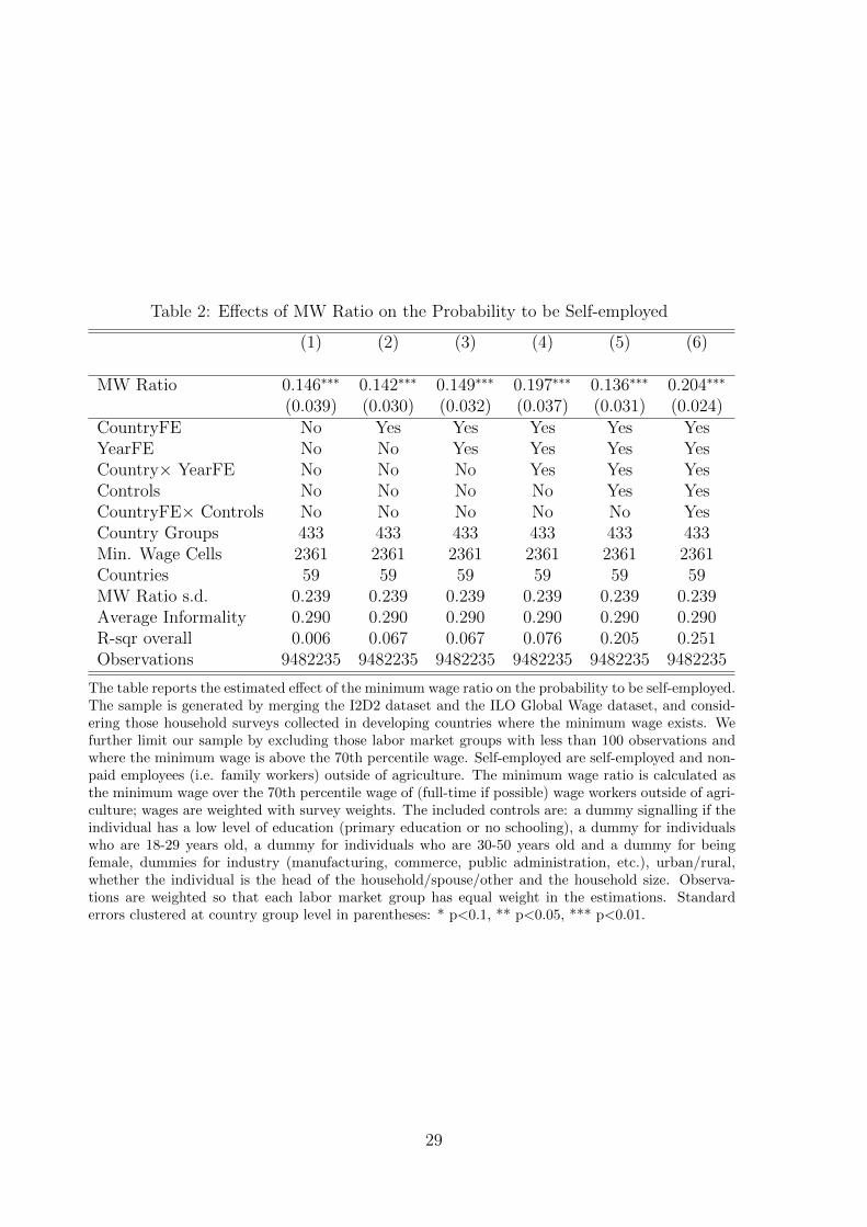
Table 2: Effects of MW Ratio on the Probability to be Self-employed
(1) (2) (3) (4) (5) (6)
MW Ratio 0.146∗∗∗ 0.142∗∗∗ 0.149∗∗∗ 0.197∗∗∗ 0.136∗∗∗ 0.204∗∗∗
(0.039) (0.030) (0.032) (0.037) (0.031) (0.024)CountryFE No Yes Yes Yes Yes YesYearFE No No Yes Yes Yes YesCountry× YearFE No No No Yes Yes YesControls No No No No Yes YesCountryFE× Controls No No No No No YesCountry Groups 433 433 433 433 433 433Min. Wage Cells 2361 2361 2361 2361 2361 2361Countries 59 59 59 59 59 59MW Ratio s.d. 0.239 0.239 0.239 0.239 0.239 0.239Average Informality 0.290 0.290 0.290 0.290 0.290 0.290R-sqr overall 0.006 0.067 0.067 0.076 0.205 0.251Observations 9482235 9482235 9482235 9482235 9482235 9482235
The table reports the estimated effect of the minimum wage ratio on the probability to be self-employed.The sample is generated by merging the I2D2 dataset and the ILO Global Wage dataset, and consid-ering those household surveys collected in developing countries where the minimum wage exists. Wefurther limit our sample by excluding those labor market groups with less than 100 observations andwhere the minimum wage is above the 70th percentile wage. Self-employed are self-employed and non-paid employees (i.e. family workers) outside of agriculture. The minimum wage ratio is calculated asthe minimum wage over the 70th percentile wage of (full-time if possible) wage workers outside of agri-culture; wages are weighted with survey weights. The included controls are: a dummy signalling if theindividual has a low level of education (primary education or no schooling), a dummy for individualswho are 18-29 years old, a dummy for individuals who are 30-50 years old and a dummy for beingfemale, dummies for industry (manufacturing, commerce, public administration, etc.), urban/rural,whether the individual is the head of the household/spouse/other and the household size. Observa-tions are weighted so that each labor market group has equal weight in the estimations. Standarderrors clustered at country group level in parentheses: * p<0.1, ** p<0.05, *** p<0.01.
29

Table 3: Effects of MW Ratio on the Probability to be Self-employed (Non-linearEffects)
(1) (2) (3) (4) (5) (6)
MW 2nd decile wages 0.040∗∗∗ 0.026∗∗ 0.029∗∗ 0.047∗∗∗ 0.027∗∗∗ 0.025∗∗∗
(0.013) (0.011) (0.011) (0.013) (0.008) (0.004)
MW 3rd decile wages 0.070∗∗∗ 0.044∗∗∗ 0.046∗∗∗ 0.071∗∗∗ 0.043∗∗∗ 0.050∗∗∗
(0.017) (0.014) (0.014) (0.017) (0.011) (0.007)
MW 4th decile wages 0.098∗∗∗ 0.055∗∗∗ 0.059∗∗∗ 0.089∗∗∗ 0.049∗∗∗ 0.063∗∗∗
(0.019) (0.017) (0.017) (0.021) (0.013) (0.009)
MW 5th decile wages 0.098∗∗∗ 0.078∗∗∗ 0.083∗∗∗ 0.117∗∗∗ 0.070∗∗∗ 0.079∗∗∗
(0.025) (0.020) (0.020) (0.024) (0.015) (0.009)
MW 6th decile wages 0.126∗∗∗ 0.094∗∗∗ 0.098∗∗∗ 0.141∗∗∗ 0.085∗∗∗ 0.096∗∗∗
(0.028) (0.023) (0.024) (0.028) (0.017) (0.011)
MW 7th decile wages 0.203∗∗∗ 0.142∗∗∗ 0.147∗∗∗ 0.193∗∗∗ 0.107∗∗∗ 0.108∗∗∗
(0.033) (0.024) (0.024) (0.027) (0.019) (0.012)
CountryFE No Yes Yes Yes Yes YesYearFE No No Yes Yes Yes YesCountry ×YearFE No No No Yes Yes YesControls No No No No Yes YesCountryFE ×Controls No No No No No YesCountry Groups 433 433 433 433 433 433Min. Wage Cells 2361 2361 2361 2361 2361 2361Countries 59 59 59 59 59 59MW Ratio s.d. 0.239 0.239 0.239 0.239 0.239 0.239Average Informality 0.290 0.290 0.290 0.290 0.290 0.290R-sqr overall 0.015 0.068 0.069 0.078 0.205 0.251Observations 9482235 9482235 9482235 9482235 9482235 9482235
The table reports the estimated effect of the minimum wage ratio on the probability to be self-employed. The sample is generated by merging the I2D2 dataset and the ILO Global Wagedataset, and considering those household surveys collected in developing countries where theminimum wage exists. We further limit our sample by excluding those labor market groups withless than 100 observations and where the minimum wage is above the 70th percentile wage. Weconsider self-employed the self-employed and non-paid employees (i.e. family workers) outside ofagriculture. MW 2nd decile wages is a dummy equal to 1 if the minimum wage is between the10th and 20th percentile of the cell wage distribution of (possibly full-time) wage workers outsideof agriculture. MW 3rd decile wages is a dummy equal to 1 if the minimum wage is between the20th and 30th percentile of the cell wage distribution of (possibly full-time) wage workers outsideagriculture , etc. The controls included are: a dummy signalling if the individual has a low levelof education (primary education or no schooling), a dummy for individuals who are 18-29 yearsold, a dummy for individuals who are 30-50 years old and a dummy for being female, dummiesfor industry (manufacturing, commerce, public administration, etc.), urban/rural, whether theindividual is the head of the household/spouse/other and the household size. In the estimationsequal weights are given to each labor market group. Standard errors clustered at country grouplevel in parentheses: * p<0.1, ** p<0.05, *** p<0.01.
30
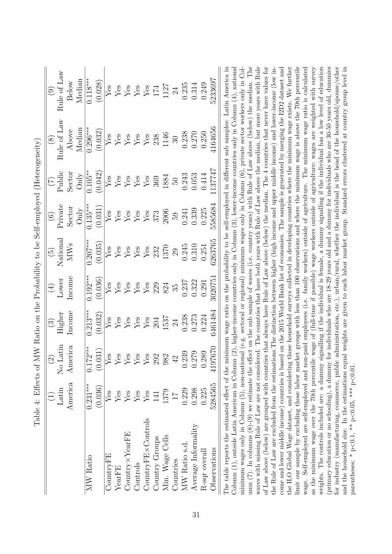
Tab
le4:
Eff
ects
ofM
WR
atio
onth
eP
robab
ilit
yto
be
Sel
f-em
plo
yed
(Het
erog
enei
ty)
(1)
(2)
(3)
(4)
(5)
(6)
(7)
(8)
(9)
Lat
inN
oL
atin
Hig
her
Low
erN
atio
nal
Pri
vate
Public
Rule
ofL
awR
ule
ofL
awA
mer
ica
Am
eric
aIn
com
eIn
com
eM
Ws
Sec
tor
Sec
tor
Ab
ove
Bel
owO
nly
Only
Med
ian
Med
ian
MW
Rat
io0.
231∗∗∗
0.17
2∗∗∗
0.21
3∗∗∗
0.19
2∗∗∗
0.20
7∗∗∗
0.13
5∗∗∗
0.10
5∗∗
0.29
6∗∗∗
0.11
8∗∗∗
(0.0
36)
(0.0
31)
(0.0
32)
(0.0
36)
(0.0
35)
(0.0
31)
(0.0
42)
(0.0
32)
(0.0
28)
Cou
ntr
yF
EY
esY
esY
esY
esY
esY
esY
esY
esY
esY
earF
EY
esY
esY
esY
esY
esY
esY
esY
esY
esC
ountr
y×
Yea
rFE
Yes
Yes
Yes
Yes
Yes
Yes
Yes
Yes
Yes
Con
trol
sY
esY
esY
esY
esY
esY
esY
esY
esY
esC
ountr
yF
E×
Con
trol
sY
esY
esY
esY
esY
esY
esY
esY
esY
esC
ountr
yG
roups
141
292
204
229
232
373
369
238
174
Min
.W
age
Cel
ls13
7998
215
3782
413
7020
0618
8411
4611
27C
ountr
ies
1742
2435
2959
5030
24M
WR
atio
s.d.
0.22
90.
239
0.23
80.
237
0.24
50.
241
0.24
30.
238
0.23
5A
vera
geIn
form
alit
y0.
298
0.27
90.
273
0.32
20.
310
0.33
90.
053
0.27
00.
314
R-s
qr
over
all
0.22
50.
289
0.22
40.
291
0.25
10.
225
0.41
40.
250
0.24
9O
bse
rvat
ions
5284
565
4197
670
6461
484
3020
751
6263
765
5585
684
1137
747
4164
656
5233
697
Th
eta
ble
rep
orts
the
esti
mat
edeff
ect
ofth
em
inim
um
wage
rati
oon
the
pro
bab
ilit
yto
be
self
-em
plo
yed
ind
iffer
ent
sub
sam
ple
s:L
ati
nA
mer
ica
inC
olu
mn
(1),
outs
ide
Lat
inA
mer
ican
inC
olu
mn
(2),
hig
her
-in
com
eco
untr
ies
on
lyin
Colu
mn
(3),
low
er-i
nco
me
cou
ntr
ies
on
lyin
Colu
mn
(4),
nati
on
al
min
imu
mw
ages
only
inC
olu
mn
(5),
non
-nat
ion
al(e
.g.
sect
ora
lor
regio
nal)
min
imu
mw
ages
on
lyin
Colu
mn
(6),
pri
vate
sect
or
work
ers
on
lyin
Col-
um
n(7
).In
colu
mn
s(8
)-(9
)w
ees
tim
ate
the
effec
ton
the
sub
sam
ple
of
wav
es(i
.e.
cou
ntr
yye
ars
)w
ith
Ru
leof
Law
ab
ove
(bel
ow)
the
med
ian
.T
he
wav
esw
ith
mis
sin
gR
ule
ofL
awar
en
otco
nsi
der
ed.
Th
eco
untr
ies
that
hav
eb
oth
years
wit
hR
ule
of
Law
ab
ove
the
med
ian
,b
ut
more
years
wit
hR
ule
ofL
awab
ove
(bel
ow)
are
grou
ped
wit
hco
untr
ies
that
alw
ays
hav
eR
ule
of
Law
ab
ove
(bel
ow)
the
med
ian
.T
he
4co
untr
ies
that
nev
erh
ave
valu
esfo
rth
eR
ule
ofL
awar
eex
clu
ded
from
the
esti
mat
ion
s.T
he
dis
tin
ctio
nb
etw
een
hig
her
(hig
hin
com
ean
du
pp
erm
iddle
inco
me)
and
low
er-i
nco
me
(low
in-
com
ean
dlo
wer
mid
dle
inco
me)
cou
ntr
ies
isb
ased
onth
e2015
Worl
dB
an
kli
stof
econom
ies.
Th
esa
mp
leis
gen
erate
dby
mer
gin
gth
eI2
D2
data
set
an
dth
eIL
OG
lob
alW
age
dat
aset
,and
con
sid
erin
gth
ose
hou
seh
old
surv
eys
coll
ecte
din
dev
elop
ing
cou
ntr
ies
wh
ere
the
min
imu
mw
age
exis
ts.
We
furt
her
lim
itou
rsa
mp
leby
excl
ud
ing
thos
ela
bor
mar
ket
grou
ps
wit
hle
ssth
an
100
ob
serv
ati
on
san
dw
her
eth
em
inim
um
wage
isab
ove
the
70th
per
centi
lew
age.
Sel
f-em
plo
yed
are
self
-em
plo
yed
and
non
-pai
dem
plo
yee
s(i
.e.
fam
ily
work
ers)
ou
tsid
eof
agri
cult
ure
.T
he
min
imu
mw
age
rati
ois
calc
ula
ted
asth
em
inim
um
wag
eov
erth
e70
thp
erce
nti
lew
age
of
(fu
ll-t
ime
ifp
oss
ible
)w
age
work
ers
ou
tsid
eof
agri
cult
ure
;w
ages
are
wei
ghte
dw
ith
surv
eyw
eigh
ts.
Th
eco
ntr
ols
incl
ud
edar
e:a
du
mm
ysi
gnal
lin
gif
the
ind
ivid
ual
isfe
male
,a
du
mm
ysi
gn
allin
gif
the
ind
ivid
ual
has
alo
wle
vel
of
edu
cati
on
(pri
mar
yed
uca
tion
orn
osc
hool
ing)
,a
du
mm
yfo
rin
div
idu
als
wh
oare
18-2
9ye
ars
old
an
da
du
mm
yfo
rin
div
idu
als
wh
oare
30-5
0ye
ars
old
,d
um
mie
sfo
rin
du
stry
(man
ufa
ctu
rin
g,co
mm
erce
,p
ub
lic
adm
inis
trati
on
,et
c.),
urb
an
/ru
ral,
whet
her
the
ind
ivid
ual
isth
eh
ead
of
the
hou
seh
old
/sp
ou
se/oth
eran
dth
eh
ouse
hol
dsi
ze.
Inth
ees
tim
atio
ns
equ
alw
eigh
tsare
giv
ento
each
lab
or
mark
etgro
up
.S
tan
dard
erro
rscl
ust
ered
at
cou
ntr
ygro
up
leve
lin
par
enth
eses
:*
p<
0.1,
**p<
0.05
,**
*p<
0.01
.
31
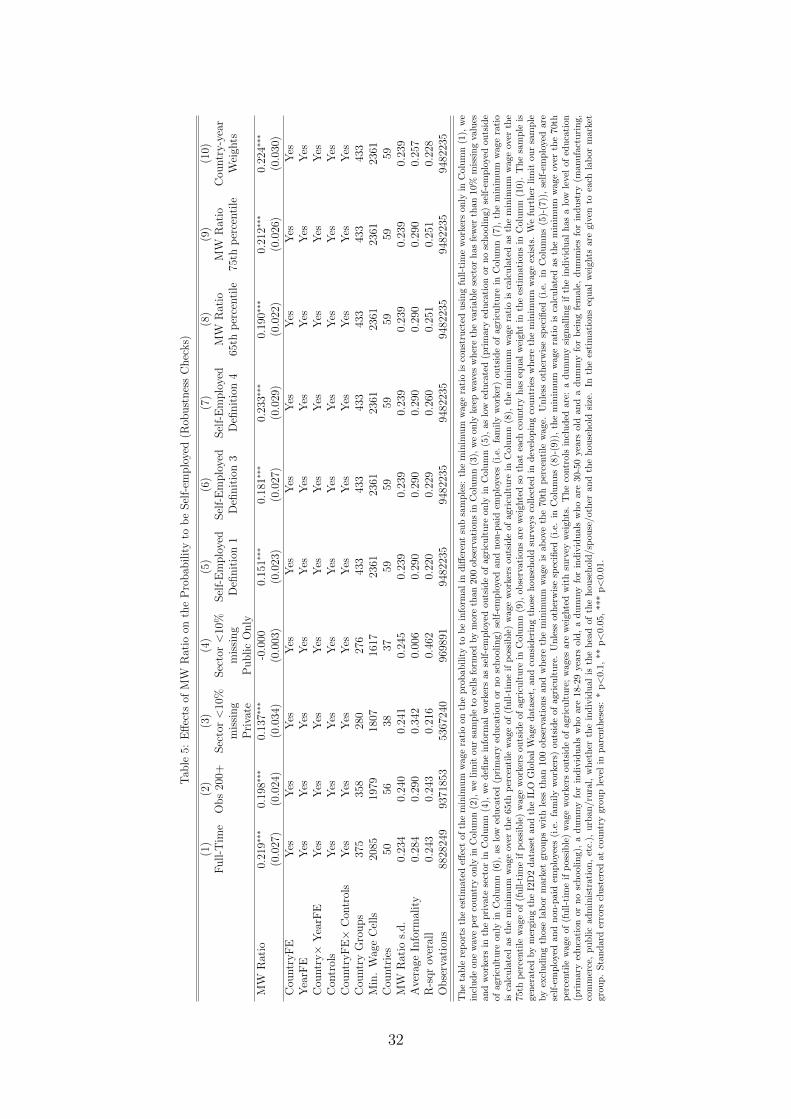
Tab
le5:
Eff
ects
ofM
WR
atio
onth
eP
robab
ilit
yto
be
Sel
f-em
plo
yed
(Rob
ust
nes
sC
hec
ks)
(1)
(2)
(3)
(4)
(5)
(6)
(7)
(8)
(9)
(10)
Full-T
ime
Obs
200+
Sec
tor<
10%
Sec
tor<
10%
Sel
f-E
mplo
yed
Sel
f-E
mplo
yed
Sel
f-E
mplo
yed
MW
Rat
ioM
WR
atio
Cou
ntr
y-y
ear
mis
sing
mis
sing
Defi
nit
ion
1D
efinit
ion
3D
efinit
ion
465
thp
erce
nti
le75
thp
erce
nti
leW
eigh
tsP
riva
teP
ublic
Only
MW
Rat
io0.
219∗∗∗
0.19
8∗∗∗
0.13
7∗∗∗
-0.0
000.
151∗∗∗
0.18
1∗∗∗
0.23
3∗∗∗
0.19
0∗∗∗
0.21
2∗∗∗
0.22
4∗∗∗
(0.0
27)
(0.0
24)
(0.0
34)
(0.0
03)
(0.0
23)
(0.0
27)
(0.0
29)
(0.0
22)
(0.0
26)
(0.0
30)
Cou
ntr
yF
EY
esY
esY
esY
esY
esY
esY
esY
esY
esY
esY
earF
EY
esY
esY
esY
esY
esY
esY
esY
esY
esY
esC
ountr
y×
Yea
rFE
Yes
Yes
Yes
Yes
Yes
Yes
Yes
Yes
Yes
Yes
Con
trol
sY
esY
esY
esY
esY
esY
esY
esY
esY
esY
esC
ountr
yF
E×
Con
trol
sY
esY
esY
esY
esY
esY
esY
esY
esY
esY
esC
ountr
yG
roups
375
358
280
276
433
433
433
433
433
433
Min
.W
age
Cel
ls20
8519
7918
0716
1723
6123
6123
6123
6123
6123
61C
ountr
ies
5056
3837
5959
5959
5959
MW
Rat
ios.
d.
0.23
40.
240
0.24
10.
245
0.23
90.
239
0.23
90.
239
0.23
90.
239
Ave
rage
Info
rmal
ity
0.28
40.
290
0.34
20.
006
0.29
00.
290
0.29
00.
290
0.29
00.
257
R-s
qr
over
all
0.24
30.
243
0.21
60.
462
0.22
00.
229
0.26
00.
251
0.25
10.
228
Obse
rvat
ions
8828
249
9371
853
5367
240
9698
9194
8223
594
8223
594
8223
594
8223
594
8223
594
8223
5
Th
eta
ble
rep
orts
the
esti
mat
edeff
ect
ofth
em
inim
um
wag
era
tio
on
the
pro
babil
ity
tob
ein
form
alin
diff
eren
tsu
bsa
mp
les:
the
min
imu
mw
age
rati
ois
con
stru
cted
usi
ng
full
-tim
ew
orke
rson
lyin
Col
um
n(1
),w
ein
clu
de
one
wav
ep
erco
untr
yon
lyin
Col
um
n(2
),w
eli
mit
our
sam
ple
toce
lls
form
edby
mor
eth
an
200
obse
rvati
on
sin
Colu
mn
(3),
we
only
keep
wav
esw
her
eth
eva
riable
sect
orh
asfe
wer
than
10%
mis
sin
gva
lues
and
wor
kers
inth
ep
riva
tese
ctor
inC
olu
mn
(4),
we
defi
ne
info
rmal
wor
kers
as
self
-em
plo
yed
outs
ide
ofagr
icu
ltu
reon
lyin
Col
um
n(5
),as
low
edu
cate
d(p
rim
ary
edu
cati
onor
no
school
ing)
self
-em
plo
yed
outs
ide
ofag
ricu
ltu
reon
lyin
Col
um
n(6
),as
low
edu
cate
d(p
rim
ary
educa
tion
or
no
sch
ooli
ng)
self
-em
plo
yed
an
dn
on-p
aid
emp
loye
es(i
.e.
fam
ily
work
er)
outs
ide
ofag
ricu
ltu
rein
Col
um
n(7
),th
em
inim
um
wag
era
tio
isca
lcu
late
das
the
min
imu
mw
age
over
the
65th
per
centi
lew
age
of
(fu
ll-t
ime
ifp
oss
ible
)w
age
wor
ker
sou
tsid
eof
agri
cult
ure
inC
olu
mn
(8),
the
min
imu
mw
age
rati
ois
calc
ula
ted
asth
em
inim
um
wag
eov
erth
e75
thp
erce
nti
lew
age
of(f
ull
-tim
eif
pos
sib
le)
wag
ew
ork
ers
outs
ide
ofagr
icu
ltu
rein
Colu
mn
(9),
obse
rvat
ion
sar
ew
eigh
ted
soth
atea
chco
untr
yh
as
equ
al
wei
ght
inth
ees
tim
atio
ns
inC
olu
mn
(10)
.T
he
sam
ple
isge
ner
ated
by
mer
gin
gth
eI2
D2
dat
aset
and
the
ILO
Glo
bal
Wag
ed
atas
et,
and
con
sid
erin
gth
ose
hou
seh
old
surv
eys
coll
ecte
din
dev
elop
ing
cou
ntr
ies
wh
ere
the
min
imu
mw
age
exis
ts.
We
furt
her
lim
itou
rsa
mp
leby
excl
ud
ing
thos
ela
bor
mar
ket
grou
ps
wit
hle
ssth
an100
obse
rvati
on
san
dw
her
eth
em
inim
um
wage
isab
ove
the
70th
per
centi
lew
age.
Un
less
oth
erw
ise
spec
ified
(i.e
.in
Col
um
ns
(5)-
(7))
,se
lf-e
mp
loye
dare
self
-em
plo
yed
and
non
-pai
dem
plo
yee
s(i
.e.
fam
ily
wor
kers
)ou
tsid
eof
agr
icu
ltu
re.
Un
less
oth
erw
ise
spec
ified
(i.e
.in
Colu
mn
s(8
)-(9
)),
the
min
imu
mw
age
rati
ois
calc
ula
ted
as
the
min
imu
mw
age
over
the
70th
per
centi
lew
age
of(f
ull
-tim
eif
pos
sib
le)
wag
ew
ork
ers
outs
ide
ofag
ricu
ltu
re;
wag
esar
ew
eighte
dw
ith
surv
eyw
eigh
ts.
Th
eco
ntr
ols
incl
ud
edar
e:a
du
mm
ysi
gnal
lin
gif
the
ind
ivid
ual
has
alo
wle
vel
ofed
uca
tion
(pri
mar
yed
uca
tion
orn
osc
hool
ing)
,a
du
mm
yfo
rin
div
idu
als
wh
oare
18-2
9ye
ars
old
,a
du
mm
yfo
rin
div
idu
als
wh
oare
30-5
0ye
ars
old
and
ad
um
my
for
bei
ng
fem
ale,
du
mm
ies
for
ind
ust
ry(m
anu
fact
uri
ng,
com
mer
ce,
pu
bli
cad
min
istr
atio
n,
etc.
),u
rban
/ru
ral,
wh
eth
erth
ein
div
idu
alis
the
hea
dof
the
hou
seh
old/sp
ou
se/o
ther
and
the
hou
seh
old
size
.In
the
esti
mat
ion
seq
ual
wei
ghts
are
give
nto
each
lab
orm
arke
tgr
oup
.S
tan
dar
der
rors
clu
ster
edat
countr
ygr
oup
leve
lin
par
enth
eses
:*
p<
0.1
,**
p<
0.05,
***
p<
0.01
.
32
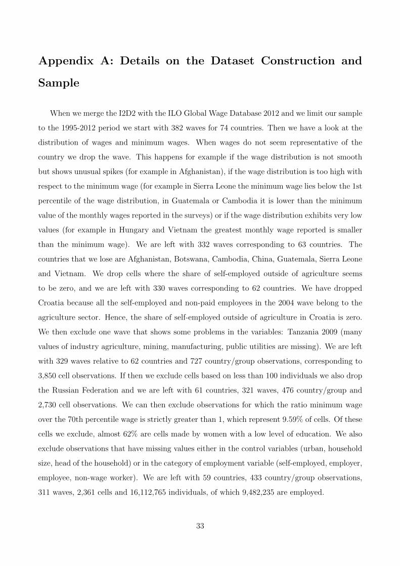
Appendix A: Details on the Dataset Construction and
Sample
When we merge the I2D2 with the ILO Global Wage Database 2012 and we limit our sample
to the 1995-2012 period we start with 382 waves for 74 countries. Then we have a look at the
distribution of wages and minimum wages. When wages do not seem representative of the
country we drop the wave. This happens for example if the wage distribution is not smooth
but shows unusual spikes (for example in Afghanistan), if the wage distribution is too high with
respect to the minimum wage (for example in Sierra Leone the minimum wage lies below the 1st
percentile of the wage distribution, in Guatemala or Cambodia it is lower than the minimum
value of the monthly wages reported in the surveys) or if the wage distribution exhibits very low
values (for example in Hungary and Vietnam the greatest monthly wage reported is smaller
than the minimum wage). We are left with 332 waves corresponding to 63 countries. The
countries that we lose are Afghanistan, Botswana, Cambodia, China, Guatemala, Sierra Leone
and Vietnam. We drop cells where the share of self-employed outside of agriculture seems
to be zero, and we are left with 330 waves corresponding to 62 countries. We have dropped
Croatia because all the self-employed and non-paid employees in the 2004 wave belong to the
agriculture sector. Hence, the share of self-employed outside of agriculture in Croatia is zero.
We then exclude one wave that shows some problems in the variables: Tanzania 2009 (many
values of industry agriculture, mining, manufacturing, public utilities are missing). We are left
with 329 waves relative to 62 countries and 727 country/group observations, corresponding to
3,850 cell observations. If then we exclude cells based on less than 100 individuals we also drop
the Russian Federation and we are left with 61 countries, 321 waves, 476 country/group and
2,730 cell observations. We can then exclude observations for which the ratio minimum wage
over the 70th percentile wage is strictly greater than 1, which represent 9.59% of cells. Of these
cells we exclude, almost 62% are cells made by women with a low level of education. We also
exclude observations that have missing values either in the control variables (urban, household
size, head of the household) or in the category of employment variable (self-employed, employer,
employee, non-wage worker). We are left with 59 countries, 433 country/group observations,
311 waves, 2,361 cells and 16,112,765 individuals, of which 9,482,235 are employed.
33
List of Countries in our Sample
Argentina 1995; Argentina 1996; Argentina 1997; Argentina 1998; Argentina 1999; Argentina
2000; Argentina 2001; Argentina 2002; Argentina 2003; Argentina 2005; Argentina 2006; Ar-
gentina 2007; Argentina 2008; Argentina 2009; Argentina 2010; Argentina 2012; Azerbaijan
1995; Burundi 1998; Burkina Faso 1998; Burkina Faso 2003; Burkina Faso 2009; Bulgaria 2001;
Bulgaria 2003; Bulgaria 2007; Bulgaria 2008; Bolivia 1997; Bolivia 1999; Bolivia 2000; Bolivia
2002; Bolivia 2003; Bolivia 2005; Bolivia 2007; Bolivia 2008; Bolivia 2009; Bolivia 2011; Bolivia
2012; Brazil 1995; Brazil 1996; Brazil 1997; Brazil 1998; Brazil 1999; Brazil 2001; Brazil 2002;
Brazil 2003; Brazil 2004; Brazil 2005; Brazil 2006; Brazil 2007; Brazil 2008; Brazil 2009; Brazil
2011; Brazil 2012; Cameroon 2001; Cameroon 2007; Colombia 1996; Colombia 1999; Colombia
2001; Colombia 2002; Colombia 2003; Colombia 2004; Colombia 2005; Colombia 2006; Colom-
bia 2007; Colombia 2008; Colombia 2009; Colombia 2010; Colombia 2011; Colombia 2012;
Costa Rica 2001; Costa Rica 2002; Costa Rica 2003; Costa Rica 2004; Costa Rica 2005; Costa
Rica 2006; Costa Rica 2007; Costa Rica 2008; Costa Rica 2009; Dominican Republic 1996; Do-
minican Republic 1997; Dominican Republic 2000; Dominican Republic 2001; Dominican Re-
public 2002; Dominican Republic 2003; Dominican Republic 2004; Dominican Republic 2005;
Dominican Republic 2006; Dominican Republic 2007; Dominican Republic 2008; Dominican
Republic 2009; Dominican Republic 2010; Dominican Republic 2011; Ecuador 2003; Ecuador
2004; Ecuador 2005; Ecuador 2006; Ecuador 2007; Ecuador 2008; Ecuador 2009; Ecuador 2010;
Ecuador 2011; Ecuador 2012; Egypt, Arab Rep. 1998; Egypt, Arab Rep. 2006; Ethiopia 2003;
Ethiopia 2004; Ethiopia 2005; Ethiopia 2006; Ethiopia 2009; Ethiopia 2010; Ethiopia 2011;
Gabon 2005; Ghana 1998; Ghana 2005; Ghana 2012; Honduras 1995; Honduras 1996; Hon-
duras 1997; Honduras 1998; Honduras 1999; Honduras 2001; Honduras 2002; Honduras 2003;
Honduras 2004; Honduras 2005; Honduras 2006; Honduras 2007; Honduras 2008; Honduras
2009; Honduras 2010; Honduras 2011; Haiti 2001; Hungary 2004; Indonesia 1996; Indonesia
1998; Indonesia 1999; Indonesia 2000; Indonesia 2001; Indonesia 2002; Indonesia 2003; Indone-
sia 2004; Indonesia 2005; Indonesia 2006; Indonesia 2010; India 1999; India 2007; Jamaica 1996;
Jamaica 1999; Jamaica 2001; Jamaica 2002; Jordan 2002; Jordan 2010; Kenya 2005; Kyrgyz
Republic 1997; Lao PDR 2002; Lao PDR 2008; Sri Lanka 1996; Sri Lanka 1998; Sri Lanka
1999; Sri Lanka 2000; Sri Lanka 2001; Sri Lanka 2003; Sri Lanka 2004; Sri Lanka 2006; Sri
Lanka 2008; Sri Lanka 2009; Latvia 2005; Latvia 2006; Latvia 2007; Latvia 2008; Morocco
34
1998; Moldova 2005; Madagascar 2001; Mexico 1996; Mexico 1998; Mexico 2000; Mexico 2002;
Mexico 2004; Mexico 2005; Mexico 2006; Mexico 2008; Mexico 2010; Mexico 2012; Malta 2009;
Malta 2010; Mongolia 2009; Mongolia 2010; Mongolia 2011; Mozambique 1996; Mozambique
2008; Mauritius 2007; Mauritius 2008; Mauritius 2009; Mauritius 2010; Mauritius 2012; Malawi
2004; Malawi 2010; Niger 2002; Nigeria 2003; Nicaragua 2005; Nicaragua 2009; Nepal 1998;
Nepal 2008; Pakistan 1999; Pakistan 2001; Pakistan 2004; Pakistan 2005; Pakistan 2006; Pak-
istan 2007; Pakistan 2008; Panama 1995; Panama 1997; Panama 1998; Panama 1999; Panama
2000; Panama 2001; Panama 2002; Panama 2003; Panama 2004; Panama 2005; Panama 2006;
Panama 2007; Panama 2008; Panama 2009; Panama 2010; Panama 2011; Panama 2012; Peru
1997; Peru 1998; Peru 1999; Peru 2000; Peru 2001; Peru 2002; Peru 2003; Peru 2004; Peru
2005; Peru 2006; Peru 2007; Peru 2008; Peru 2009; Peru 2010; Peru 2011; Peru 2012; Philip-
pines 2001; Philippines 2002; Philippines 2003; Philippines 2004; Philippines 2005; Philippines
2006; Philippines 2007; Philippines 2008; Philippines 2009; Philippines 2010; Philippines 2011;
Paraguay 1995; Paraguay 1997; Paraguay 1999; Paraguay 2001; Paraguay 2002; Paraguay 2003;
Paraguay 2004; Paraguay 2006; Paraguay 2007; Paraguay 2008; Paraguay 2009; Paraguay 2010;
Rwanda 2005; Rwanda 2010; Solomon Islands 2005; El Salvador 1995; El Salvador 1996; El
Salvador 1998; El Salvador 1999; El Salvador 2000; El Salvador 2001; El Salvador 2006; El
Salvador 2007; Serbia 2008; Chad 2003; Thailand 2000; Thailand 2002; Thailand 2006; Thai-
land 2009; Tajikistan 1999; Tajikistan 2003; Tunisia 2000; Turkey 2005; Turkey 2006; Turkey
2007; Turkey 2008; Turkey 2009; Turkey 2010; Tanzania 2006; Uganda 2005; Uruguay 1995;
Uruguay 1996; Uruguay 1997; Uruguay 1998; Uruguay 2000; Uruguay 2001; Uruguay 2002;
Uruguay 2003; Uruguay 2004; Uruguay 2005; Uruguay 2006; Uruguay 2007; Uruguay 2008;
Uruguay 2009; Uruguay 2010; Uruguay 2011; Uruguay 2012; Venezuela, RB 1995; Venezuela,
RB 1998; Venezuela, RB 2000; Venezuela, RB 2001; Venezuela, RB 2002; Venezuela, RB 2003;
Venezuela, RB 2004; Venezuela, RB 2005; Venezuela, RB 2006; Zambia 2010.
Appendix B: Additional Figures and Tables
35
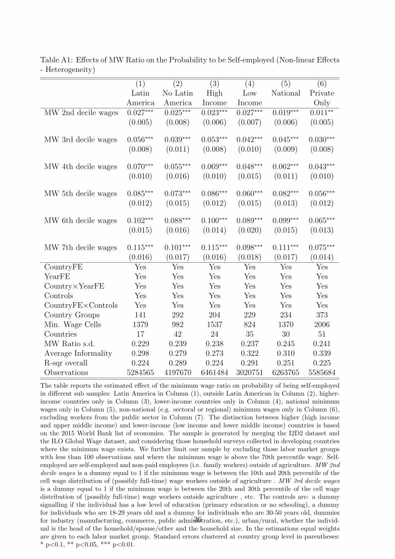
Table A1: Effects of MW Ratio on the Probability to be Self-employed (Non-linear Effects- Heterogeneity)
(1) (2) (3) (4) (5) (6)Latin No Latin High Low National Private
America America Income Income OnlyMW 2nd decile wages 0.027∗∗∗ 0.025∗∗∗ 0.023∗∗∗ 0.027∗∗∗ 0.019∗∗∗ 0.011∗∗
(0.005) (0.008) (0.006) (0.007) (0.006) (0.005)
MW 3rd decile wages 0.056∗∗∗ 0.039∗∗∗ 0.053∗∗∗ 0.042∗∗∗ 0.045∗∗∗ 0.030∗∗∗
(0.008) (0.011) (0.008) (0.010) (0.009) (0.008)
MW 4th decile wages 0.070∗∗∗ 0.055∗∗∗ 0.069∗∗∗ 0.048∗∗∗ 0.062∗∗∗ 0.043∗∗∗
(0.010) (0.016) (0.010) (0.015) (0.011) (0.010)
MW 5th decile wages 0.085∗∗∗ 0.073∗∗∗ 0.086∗∗∗ 0.060∗∗∗ 0.082∗∗∗ 0.056∗∗∗
(0.012) (0.015) (0.012) (0.015) (0.013) (0.012)
MW 6th decile wages 0.102∗∗∗ 0.088∗∗∗ 0.100∗∗∗ 0.089∗∗∗ 0.099∗∗∗ 0.065∗∗∗
(0.015) (0.016) (0.014) (0.020) (0.015) (0.013)
MW 7th decile wages 0.115∗∗∗ 0.101∗∗∗ 0.115∗∗∗ 0.098∗∗∗ 0.111∗∗∗ 0.075∗∗∗
(0.016) (0.017) (0.016) (0.018) (0.017) (0.014)CountryFE Yes Yes Yes Yes Yes YesYearFE Yes Yes Yes Yes Yes YesCountry×YearFE Yes Yes Yes Yes Yes YesControls Yes Yes Yes Yes Yes YesCountryFE×Controls Yes Yes Yes Yes Yes YesCountry Groups 141 292 204 229 234 373Min. Wage Cells 1379 982 1537 824 1370 2006Countries 17 42 24 35 30 51MW Ratio s.d. 0.229 0.239 0.238 0.237 0.245 0.241Average Informality 0.298 0.279 0.273 0.322 0.310 0.339R-sqr overall 0.224 0.289 0.224 0.291 0.251 0.225Observations 5284565 4197670 6461484 3020751 6263765 5585684
The table reports the estimated effect of the minimum wage ratio on probability of being self-employedin different sub samples: Latin America in Column (1), outside Latin American in Column (2), higher-income countries only in Column (3), lower-income countries only in Column (4), national minimumwages only in Column (5), non-national (e.g. sectoral or regional) minimum wages only in Column (6),excluding workers from the public sector in Column (7). The distinction between higher (high incomeand upper middle income) and lower-income (low income and lower middle income) countries is basedon the 2015 World Bank list of economies. The sample is generated by merging the I2D2 dataset andthe ILO Global Wage dataset, and considering those household surveys collected in developing countrieswhere the minimum wage exists. We further limit our sample by excluding those labor market groupswith less than 100 observations and where the minimum wage is above the 70th percentile wage. Self-employed are self-employed and non-paid employees (i.e. family workers) outside of agriculture. MW 2nddecile wages is a dummy equal to 1 if the minimum wage is between the 10th and 20th percentile of thecell wage distribution of (possibly full-time) wage workers outside of agriculture . MW 3rd decile wagesis a dummy equal to 1 if the minimum wage is between the 20th and 30th percentile of the cell wagedistribution of (possibly full-time) wage workers outside agriculture , etc. The controls are: a dummysignalling if the individual has a low level of education (primary education or no schooling), a dummyfor individuals who are 18-29 years old and a dummy for individuals who are 30-50 years old, dummiesfor industry (manufacturing, commerce, public administration, etc.), urban/rural, whether the individ-ual is the head of the household/spouse/other and the household size. In the estimations equal weightsare given to each labor market group. Standard errors clustered at country group level in parentheses:* p<0.1, ** p<0.05, *** p<0.01.
36
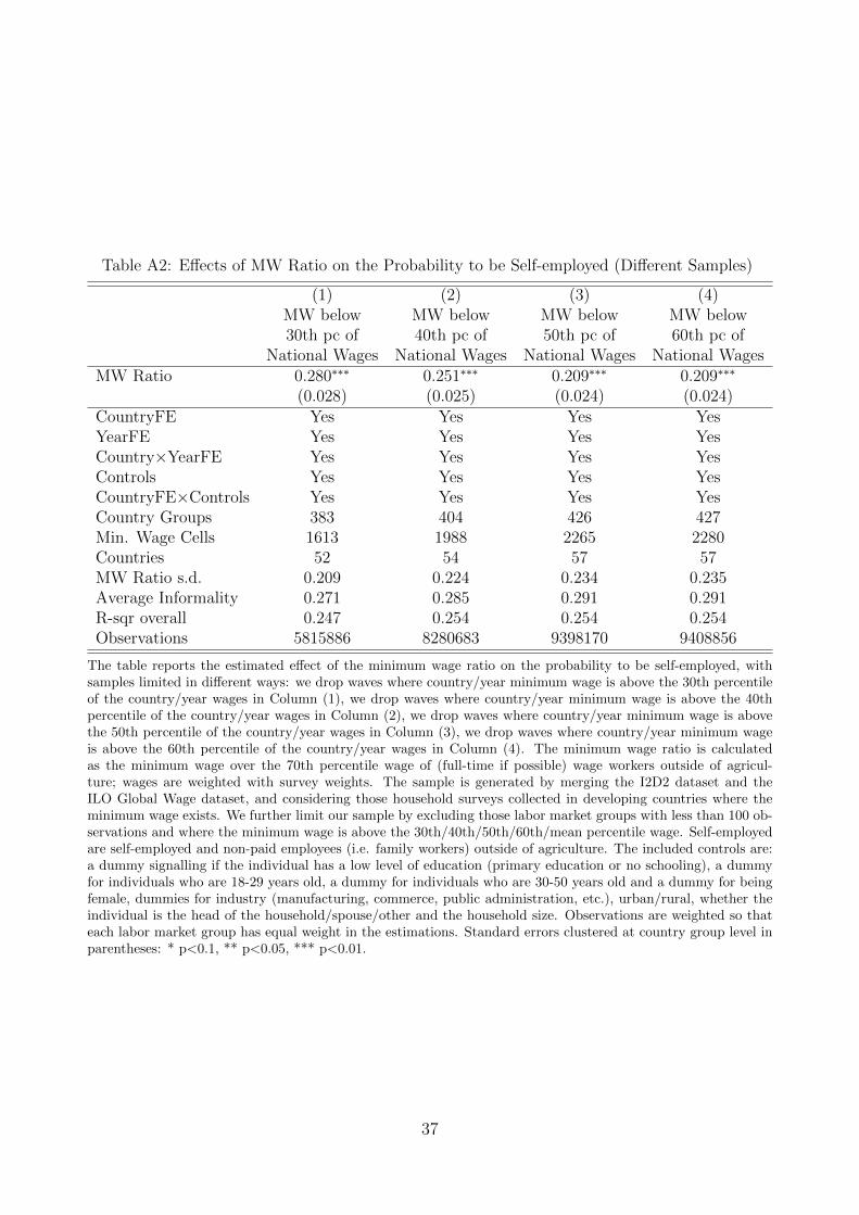
Table A2: Effects of MW Ratio on the Probability to be Self-employed (Different Samples)
(1) (2) (3) (4)MW below MW below MW below MW below30th pc of 40th pc of 50th pc of 60th pc of
National Wages National Wages National Wages National WagesMW Ratio 0.280∗∗∗ 0.251∗∗∗ 0.209∗∗∗ 0.209∗∗∗
(0.028) (0.025) (0.024) (0.024)CountryFE Yes Yes Yes YesYearFE Yes Yes Yes YesCountry×YearFE Yes Yes Yes YesControls Yes Yes Yes YesCountryFE×Controls Yes Yes Yes YesCountry Groups 383 404 426 427Min. Wage Cells 1613 1988 2265 2280Countries 52 54 57 57MW Ratio s.d. 0.209 0.224 0.234 0.235Average Informality 0.271 0.285 0.291 0.291R-sqr overall 0.247 0.254 0.254 0.254Observations 5815886 8280683 9398170 9408856
The table reports the estimated effect of the minimum wage ratio on the probability to be self-employed, withsamples limited in different ways: we drop waves where country/year minimum wage is above the 30th percentileof the country/year wages in Column (1), we drop waves where country/year minimum wage is above the 40thpercentile of the country/year wages in Column (2), we drop waves where country/year minimum wage is abovethe 50th percentile of the country/year wages in Column (3), we drop waves where country/year minimum wageis above the 60th percentile of the country/year wages in Column (4). The minimum wage ratio is calculatedas the minimum wage over the 70th percentile wage of (full-time if possible) wage workers outside of agricul-ture; wages are weighted with survey weights. The sample is generated by merging the I2D2 dataset and theILO Global Wage dataset, and considering those household surveys collected in developing countries where theminimum wage exists. We further limit our sample by excluding those labor market groups with less than 100 ob-servations and where the minimum wage is above the 30th/40th/50th/60th/mean percentile wage. Self-employedare self-employed and non-paid employees (i.e. family workers) outside of agriculture. The included controls are:a dummy signalling if the individual has a low level of education (primary education or no schooling), a dummyfor individuals who are 18-29 years old, a dummy for individuals who are 30-50 years old and a dummy for beingfemale, dummies for industry (manufacturing, commerce, public administration, etc.), urban/rural, whether theindividual is the head of the household/spouse/other and the household size. Observations are weighted so thateach labor market group has equal weight in the estimations. Standard errors clustered at country group level inparentheses: * p<0.1, ** p<0.05, *** p<0.01.
37
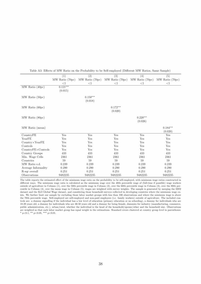
Table A3: Effects of MW Ratio on the Probability to be Self-employed (Different MW Ratios, Same Sample)
(1) (2) (3) (4) (5)MW Ratio (70pc) MW Ratio (70pc) MW Ratio (70pc) MW Ratio (70pc) MW Ratio (70pc)
<1 <1 <1 <1 <1MW Ratio (40pc) 0.121∗∗∗
(0.015)
MW Ratio (50pc) 0.150∗∗∗
(0.018)
MW Ratio (60pc) 0.172∗∗∗
(0.020)
MW Ratio (80pc) 0.220∗∗∗
(0.026)
MW Ratio (mean) 0.184∗∗∗
(0.020)CountryFE Yes Yes Yes Yes YesYearFE Yes Yes Yes Yes YesCountry×YearFE Yes Yes Yes Yes YesControls Yes Yes Yes Yes YesCountryFE×Controls Yes Yes Yes Yes YesCountry Groups 433 433 433 433 433Min. Wage Cells 2361 2361 2361 2361 2361Countries 59 59 59 59 59MW Ratio s.d. 0.239 0.239 0.239 0.239 0.239Average Informality 0.290 0.290 0.290 0.290 0.290R-sqr overall 0.251 0.251 0.251 0.251 0.251Observations 9482235 9482235 9482235 9482235 9482235
The table reports the estimated effect of the minimum wage ratio on the probability to be self-employed, with minimum wage ratios constructed indifferent ways. The minimum wage ratio is calculated as the minimum wage over the 40th percentile wage of (full-time if possible) wage workersoutside of agriculture in Column (1), over the 50th percentile wage in Column (2), over the 60th percentile wage in Column (3), over the 80th per-centile in Column (4), over the mean wage in Column (5); wages are weighted with survey weights. The sample is generated by merging the I2D2dataset and the ILO Global Wage dataset, and considering those household surveys collected in developing countries where the minimum wage ex-ists. We further limit our sample by excluding those labor market groups with less than 100 observations and where the minimum wage is abovethe 70th percentile wage. Self-employed are self-employed and non-paid employees (i.e. family workers) outside of agriculture. The included con-trols are: a dummy signalling if the individual has a low level of education (primary education or no schooling), a dummy for individuals who are18-29 years old, a dummy for individuals who are 30-50 years old and a dummy for being female, dummies for industry (manufacturing, commerce,public administration, etc.), urban/rural, whether the individual is the head of the household/spouse/other and the household size. Observationsare weighted so that each labor market group has equal weight in the estimations. Standard errors clustered at country group level in parentheses:* p<0.1, ** p<0.05, *** p<0.01.
38
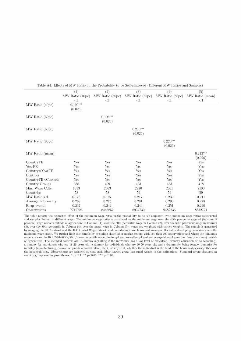
Table A4: Effects of MW Ratio on the Probability to be Self-employed (Different MW Ratios and Samples)
(1) (2) (3) (4) (5)MW Ratio (40pc) MW Ratio (50pc) MW Ratio (60pc) MW Ratio (80pc) MW Ratio (mean)
<1 <1 <1 <1 <1MW Ratio (40pc) 0.190∗∗∗
(0.026)
MW Ratio (50pc) 0.195∗∗∗
(0.025)
MW Ratio (60pc) 0.210∗∗∗
(0.026)
MW Ratio (80pc) 0.220∗∗∗
(0.026)
MW Ratio (mean) 0.213∗∗∗
(0.026)CountryFE Yes Yes Yes Yes YesYearFE Yes Yes Yes Yes YesCountry×YearFE Yes Yes Yes Yes YesControls Yes Yes Yes Yes YesCountryFE×Controls Yes Yes Yes Yes YesCountry Groups 388 409 423 433 418Min. Wage Cells 1853 2063 2220 2361 2180Countries 58 58 59 59 59MW Ratio s.d. 0.176 0.197 0.217 0.239 0.211Average Informality 0.269 0.275 0.281 0.290 0.278R-sqr overall 0.237 0.242 0.244 0.251 0.240Observations 7712726 8466852 8934730 9482235 8832721
The table reports the estimated effect of the minimum wage ratio on the probability to be self-employed, with minimum wage ratios constructedand samples limited in different ways. The minimum wage ratio is calculated as the minimum wage over the 40th percentile wage of (full-time ifpossible) wage workers outside of agriculture in Column (1), over the 50th percentile wage in Column (2), over the 60th percentile wage in Column(3), over the 80th percentile in Column (4), over the mean wage in Column (5); wages are weighted with survey weights. The sample is generatedby merging the I2D2 dataset and the ILO Global Wage dataset, and considering those household surveys collected in developing countries where theminimum wage exists. We further limit our sample by excluding those labor market groups with less than 100 observations and where the minimumwage is above the 40th/50th/60th/80th/mean percentile wage. Self-employed are self-employed and non-paid employees (i.e. family workers) outsideof agriculture. The included controls are: a dummy signalling if the individual has a low level of education (primary education or no schooling),a dummy for individuals who are 18-29 years old, a dummy for individuals who are 30-50 years old and a dummy for being female, dummies forindustry (manufacturing, commerce, public administration, etc.), urban/rural, whether the individual is the head of the household/spouse/other andthe household size. Observations are weighted so that each labor market group has equal weight in the estimations. Standard errors clustered atcountry group level in parentheses: * p<0.1, ** p<0.05, *** p<0.01.
39
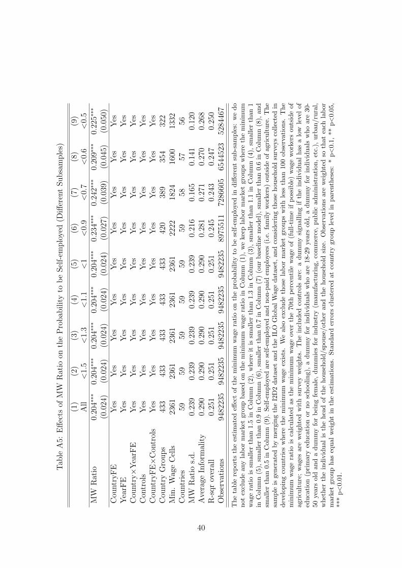
Tab
leA
5:E
ffec
tsof
MW
Rat
ioon
the
Pro
bab
ilit
yto
be
Sel
f-em
plo
yed
(Diff
eren
tSubsa
mple
s)
(1)
(2)
(3)
(4)
(5)
(6)
(7)
(8)
(9)
All
<1.
5<
1.3
<1.
1<
1<
0.9
<0.
7<
0.6
<0.
5M
WR
atio
0.20
4∗∗∗
0.20
4∗∗∗
0.20
4∗∗∗
0.20
4∗∗∗
0.20
4∗∗∗
0.23
4∗∗∗
0.24
2∗∗∗
0.20
9∗∗∗
0.22
5∗∗∗
(0.0
24)
(0.0
24)
(0.0
24)
(0.0
24)
(0.0
24)
(0.0
27)
(0.0
39)
(0.0
45)
(0.0
50)
Cou
ntr
yF
EY
esY
esY
esY
esY
esY
esY
esY
esY
esY
earF
EY
esY
esY
esY
esY
esY
esY
esY
esY
esC
ountr
y×
Yea
rFE
Yes
Yes
Yes
Yes
Yes
Yes
Yes
Yes
Yes
Con
trol
sY
esY
esY
esY
esY
esY
esY
esY
esY
esC
ountr
yF
E×
Con
trol
sY
esY
esY
esY
esY
esY
esY
esY
esY
esC
ountr
yG
roups
433
433
433
433
433
420
389
354
322
Min
.W
age
Cel
ls23
6123
6123
6123
6123
6122
2218
2416
0013
32C
ountr
ies
5959
5959
5959
5857
56M
WR
atio
s.d.
0.23
90.
239
0.23
90.
239
0.23
90.
216
0.16
50.
141
0.12
0A
vera
geIn
form
alit
y0.
290
0.29
00.
290
0.29
00.
290
0.28
10.
271
0.27
00.
268
R-s
qr
over
all
0.25
10.
251
0.25
10.
251
0.25
10.
245
0.24
30.
247
0.25
0O
bse
rvat
ions
9482
235
9482
235
9482
235
9482
235
9482
235
8975
511
7286
605
6544
523
5284
467
Th
eta
ble
rep
orts
the
esti
mat
edeff
ect
ofth
em
inim
um
wage
rati
oon
the
pro
bab
ilit
yto
be
self
-em
plo
yed
ind
iffer
ent
sub
-sam
ple
s:w
ed
on
otex
clu
de
any
lab
orm
arket
grou
pb
ased
onth
em
inim
um
wage
rati
oin
Colu
mn
(1),
we
keep
lab
or
mark
etgro
up
sw
her
eth
em
inim
um
wag
era
tio
issm
alle
rth
an1.
5in
Col
um
n(2
),w
her
eit
issm
all
erth
an
1.3
inC
olu
mn
(3),
small
erth
an
1.1
inC
olu
mn
(4),
small
erth
an
1in
Col
um
n(5
),sm
alle
rth
an0.
9in
Col
um
n(6
),sm
alle
rth
an
0.7
inC
olu
mn
(7)
(ou
rb
ase
lin
em
od
el),
small
erth
an
0.6
inC
olu
mn
(8),
an
dsm
alle
rth
an0.
5in
Col
um
n(9
).S
elf-
emp
loye
dar
ese
lf-e
mp
loye
dan
dn
on
-paid
emp
loyee
s(i
.e.
fam
ily
work
ers)
ou
tsid
eof
agri
cult
ure
.T
he
sam
ple
isge
ner
ated
by
mer
gin
gth
eI2
D2
dat
aset
and
the
ILO
Glo
bal
Wage
data
set,
an
dco
nsi
der
ing
those
hou
seh
old
surv
eys
coll
ecte
din
dev
elop
ing
cou
ntr
ies
wh
ere
the
min
imu
mw
age
exis
ts.
We
als
oex
clud
eth
ose
lab
or
mark
etgro
up
sw
ith
less
than
100
ob
serv
ati
on
s.T
he
min
imu
mw
age
rati
ois
calc
ula
ted
asth
em
inim
um
wag
eov
erth
e70th
per
centi
lew
age
of
(fu
ll-t
ime
ifp
oss
ible
)w
age
work
ers
ou
tsid
eof
agri
cult
ure
;w
ages
are
wei
ghte
dw
ith
surv
eyw
eigh
ts.
The
incl
ud
edco
ntr
ols
are
:a
du
mm
ysi
gn
all
ing
ifth
ein
div
idu
al
has
alo
wle
vel
of
edu
cati
on(p
rim
ary
edu
cati
onor
no
sch
ool
ing)
,a
du
mm
yfo
rin
div
idu
als
wh
oare
18-2
9yea
rsold
,a
du
mm
yfo
rin
div
idu
als
wh
oare
30-
50ye
ars
old
and
ad
um
my
for
bei
ng
fem
ale,
du
mm
ies
for
ind
ust
ry(m
anu
fact
uri
ng,
com
mer
ce,
pu
bli
cad
min
istr
ati
on
,et
c.),
urb
an
/ru
ral,
wh
eth
erth
ein
div
idu
alis
the
hea
dof
the
hou
seh
old
/sp
ou
se/oth
eran
dth
eh
ou
seh
old
size
.O
bse
rvati
on
sare
wei
ghte
dso
that
each
lab
or
mar
ket
grou
ph
aseq
ual
wei
ght
inth
ees
tim
atio
ns.
Sta
nd
ard
erro
rscl
ust
ered
at
cou
ntr
ygro
up
leve
lin
pare
nth
eses
:*
p<
0.1
,**
p<
0.0
5,
***
p<
0.01
.
40
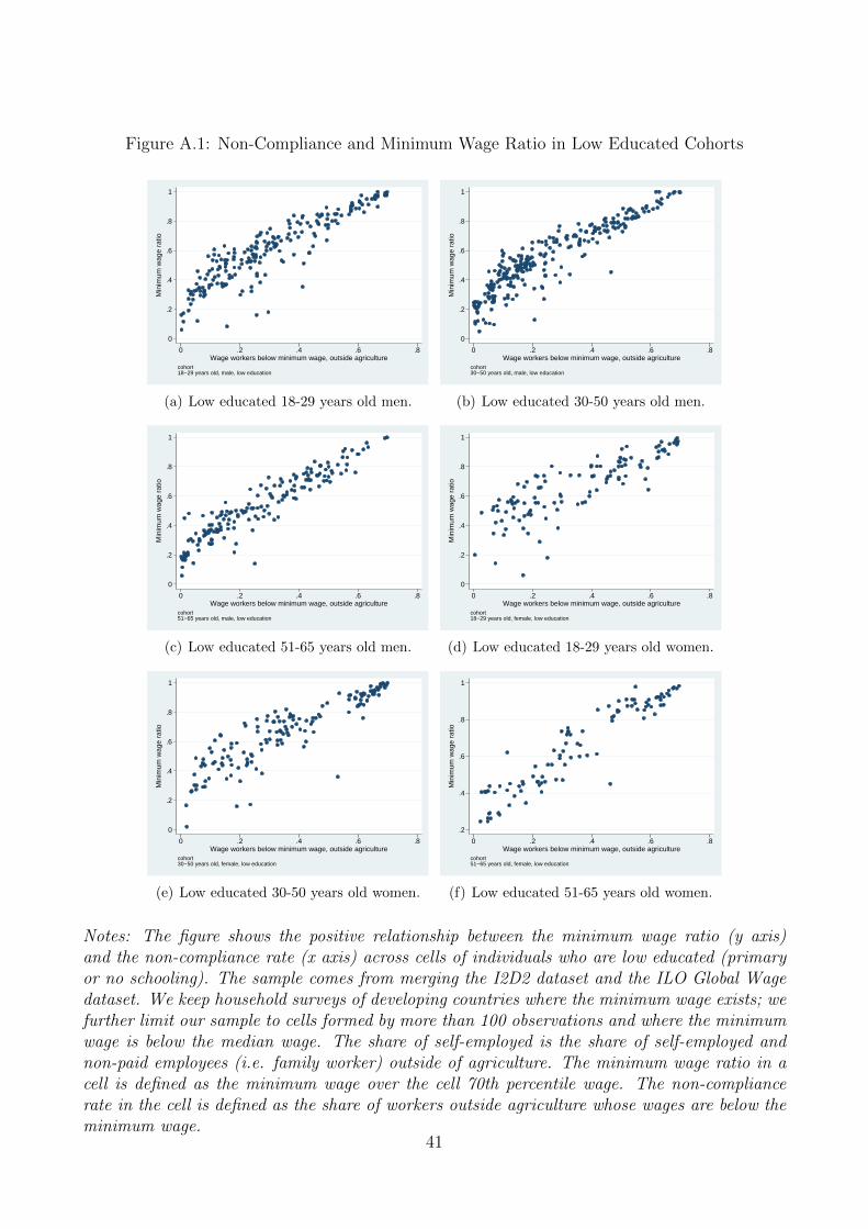
Figure A.1: Non-Compliance and Minimum Wage Ratio in Low Educated Cohorts
0
.2
.4
.6
.8
1
Min
imum
wag
e ra
tio
0 .2 .4 .6 .8Wage workers below minimum wage, outside agriculture
cohort18−29 years old, male, low education
(a) Low educated 18-29 years old men.
0
.2
.4
.6
.8
1
Min
imum
wag
e ra
tio
0 .2 .4 .6 .8Wage workers below minimum wage, outside agriculture
cohort30−50 years old, male, low education
(b) Low educated 30-50 years old men.
0
.2
.4
.6
.8
1
Min
imum
wag
e ra
tio
0 .2 .4 .6 .8Wage workers below minimum wage, outside agriculture
cohort51−65 years old, male, low education
(c) Low educated 51-65 years old men.
0
.2
.4
.6
.8
1
Min
imum
wag
e ra
tio
0 .2 .4 .6 .8Wage workers below minimum wage, outside agriculture
cohort18−29 years old, female, low education
(d) Low educated 18-29 years old women.
0
.2
.4
.6
.8
1
Min
imum
wag
e ra
tio
0 .2 .4 .6 .8Wage workers below minimum wage, outside agriculture
cohort30−50 years old, female, low education
(e) Low educated 30-50 years old women.
.2
.4
.6
.8
1
Min
imum
wag
e ra
tio
0 .2 .4 .6 .8Wage workers below minimum wage, outside agriculture
cohort51−65 years old, female, low education
(f) Low educated 51-65 years old women.
Notes: The figure shows the positive relationship between the minimum wage ratio (y axis)and the non-compliance rate (x axis) across cells of individuals who are low educated (primaryor no schooling). The sample comes from merging the I2D2 dataset and the ILO Global Wagedataset. We keep household surveys of developing countries where the minimum wage exists; wefurther limit our sample to cells formed by more than 100 observations and where the minimumwage is below the median wage. The share of self-employed is the share of self-employed andnon-paid employees (i.e. family worker) outside of agriculture. The minimum wage ratio in acell is defined as the minimum wage over the cell 70th percentile wage. The non-compliancerate in the cell is defined as the share of workers outside agriculture whose wages are below theminimum wage.
41
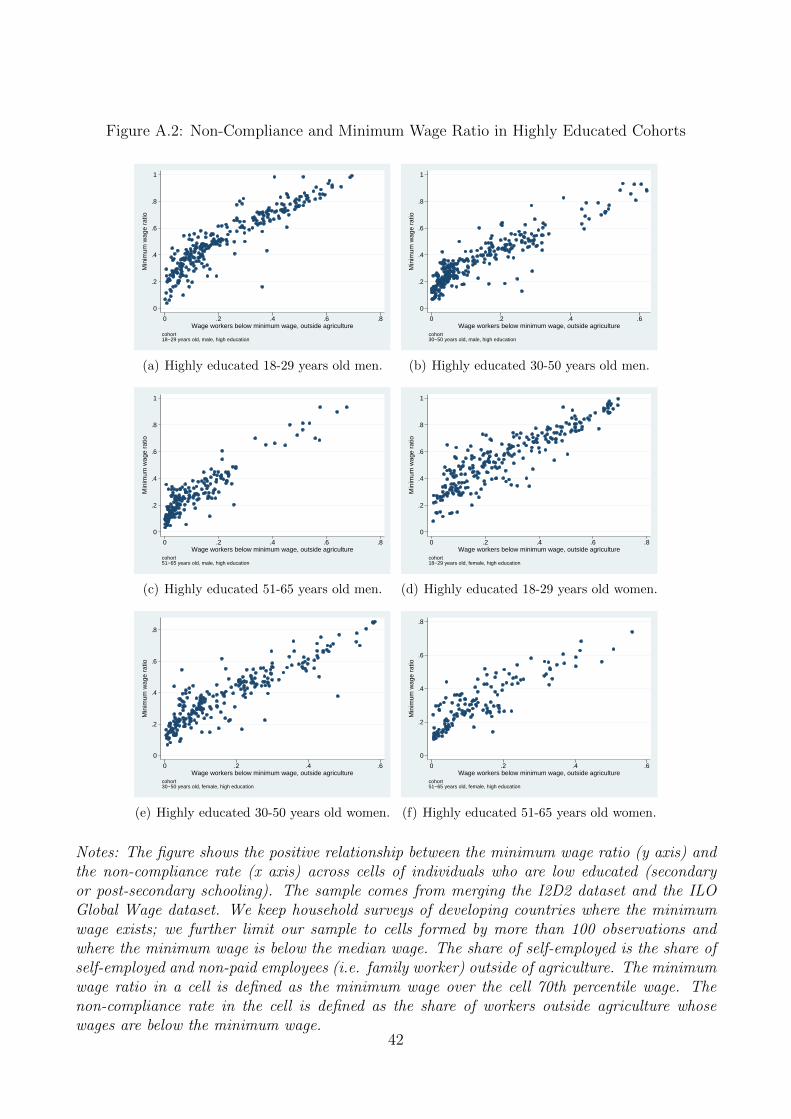
Figure A.2: Non-Compliance and Minimum Wage Ratio in Highly Educated Cohorts
0
.2
.4
.6
.8
1
Min
imum
wag
e ra
tio
0 .2 .4 .6 .8Wage workers below minimum wage, outside agriculture
cohort18−29 years old, male, high education
(a) Highly educated 18-29 years old men.
0
.2
.4
.6
.8
1
Min
imum
wag
e ra
tio
0 .2 .4 .6Wage workers below minimum wage, outside agriculture
cohort30−50 years old, male, high education
(b) Highly educated 30-50 years old men.
0
.2
.4
.6
.8
1
Min
imum
wag
e ra
tio
0 .2 .4 .6 .8Wage workers below minimum wage, outside agriculture
cohort51−65 years old, male, high education
(c) Highly educated 51-65 years old men.
0
.2
.4
.6
.8
1
Min
imum
wag
e ra
tio
0 .2 .4 .6 .8Wage workers below minimum wage, outside agriculture
cohort18−29 years old, female, high education
(d) Highly educated 18-29 years old women.
0
.2
.4
.6
.8
Min
imum
wag
e ra
tio
0 .2 .4 .6Wage workers below minimum wage, outside agriculture
cohort30−50 years old, female, high education
(e) Highly educated 30-50 years old women.
0
.2
.4
.6
.8
Min
imum
wag
e ra
tio
0 .2 .4 .6Wage workers below minimum wage, outside agriculture
cohort51−65 years old, female, high education
(f) Highly educated 51-65 years old women.
Notes: The figure shows the positive relationship between the minimum wage ratio (y axis) andthe non-compliance rate (x axis) across cells of individuals who are low educated (secondaryor post-secondary schooling). The sample comes from merging the I2D2 dataset and the ILOGlobal Wage dataset. We keep household surveys of developing countries where the minimumwage exists; we further limit our sample to cells formed by more than 100 observations andwhere the minimum wage is below the median wage. The share of self-employed is the share ofself-employed and non-paid employees (i.e. family worker) outside of agriculture. The minimumwage ratio in a cell is defined as the minimum wage over the cell 70th percentile wage. Thenon-compliance rate in the cell is defined as the share of workers outside agriculture whosewages are below the minimum wage.
42