mihail pivtoraiko 1. motion planning the challenge: reliable autonomous robots 2 navlab, 1985 boss,...

1

A Survey ofDifferentially Constrained

PlanningMihail Pivtoraiko

2

Motion Planning

The Challenge:Reliable Autonomous Robots

NavLab, 1985

Boss, 2007MER, 2004Crusher, 2006

ALV, 1988

XUV, 1998

Stanford Cart, 1979

Agenda

3

• Deterministic planners– Path smoothing– Control sampling– State sampling

• Randomized planners– Probabilistic roadmaps– Rapidly exploring Random

Trees

Motivation

4

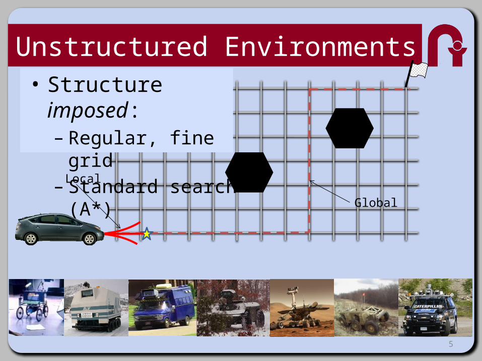
Local

Global

ALV (Daily et al., 1988)

Unstructured Environments

5

Local

Global

• Structure imposed:– Regular, fine grid– Standard search (A*)

6

Global

?

Unstructured and Uncertain• Uncertain terrain– Potentially changing

Local

7

Global

?

Unstructured and Uncertain• Unseen obstacles– Detected up close– Invalidate the plan

Local

8

Global

?

Unstructured and Uncertain

Efficient replanning

D*/Smarty (Stentz & Hebert, 1994)Ranger (Kelly, 1995)Morphin (Simmons et al., 1996)Gestalt (Maimone et al., 2002)

Local

9

Mobility Constraints• 2D global planners lead to

nonconvergence in difficult environments

• Robot will fail to make the turn into the corridor

• Global planner must understand the need to swing wide

• Issues:– Passage missed, or– Point-turn is necessary…

Plan Step n

Plan Step n+1

Plan Step n+2

10

In the Field…PerceptOR/UPI, 2005 Rover Navigation, 2008

11

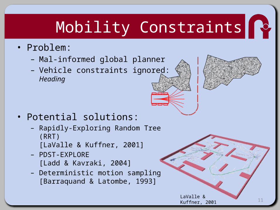
Mobility Constraints• Problem:

– Mal-informed global planner– Vehicle constraints ignored:

Heading

• Potential solutions:– Rapidly-Exploring Random Tree (RRT)

[LaValle & Kuffner, 2001]– PDST-EXPLORE

[Ladd & Kavraki, 2004]– Deterministic motion sampling

[Barraquand & Latombe, 1993]

LaValle & Kuffner, 2001

12

Mobility Constraints

Bruntingthorpe Proving Grounds Leicestershire, UK

April 1999

13

Extreme Maneuvering

Kolter et al., 2010

14

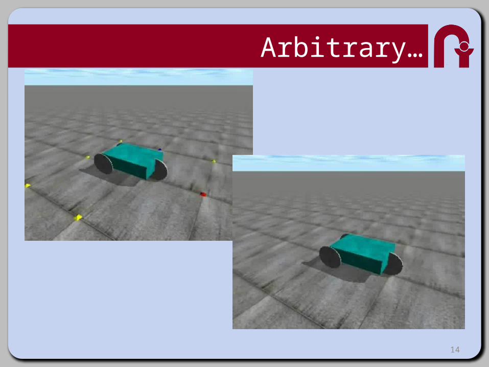
Arbitrary…

15

Dynamics Planning

16

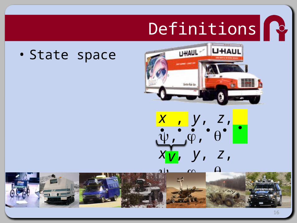
Definitions• State space

x , y, z, , , x , y, z, , ,

v

17

Definitions• State space• Control space– Accelerator– Steering

x , y, z, , , x , y, z, , ,

v

18

Definitions• State space• Control space• Feasibility– Satisfaction of

differential constraints– General formulation x = f(x, u, t)

19

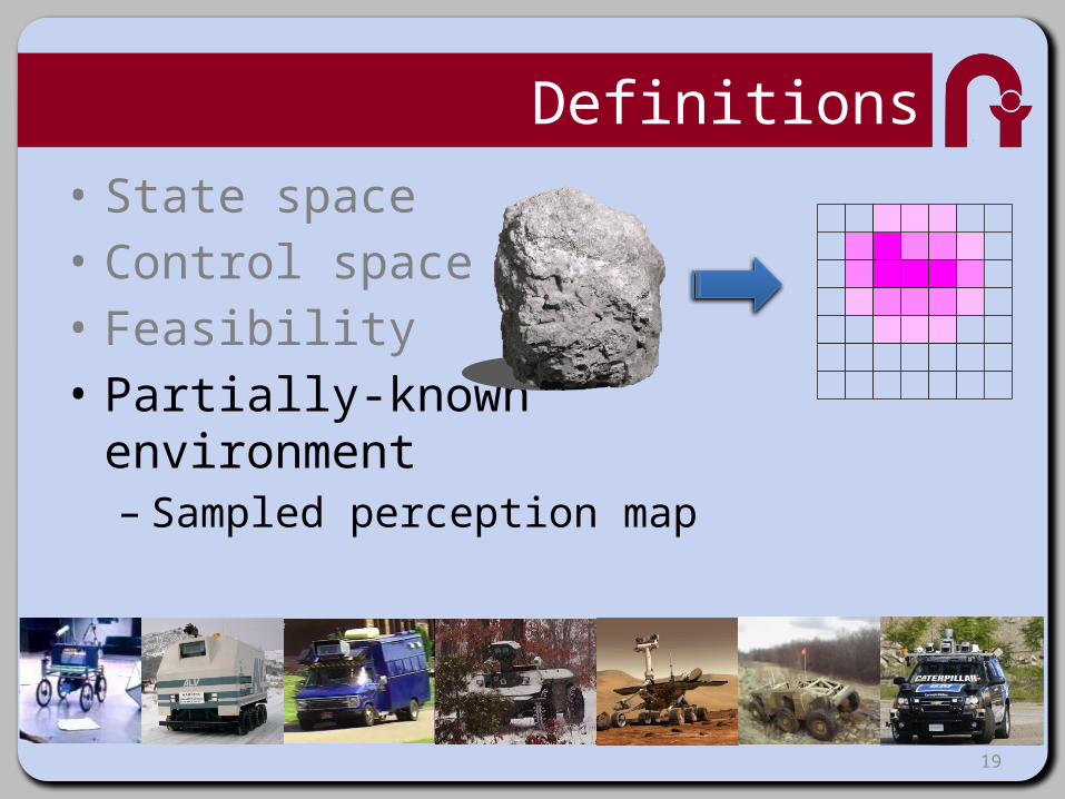
Definitions• State space• Control space• Feasibility• Partially-known

environment– Sampled perception map

20

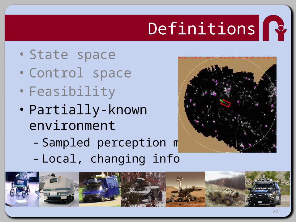
Definitions• State space• Control space• Feasibility• Partially-known

environment– Sampled perception map– Local, changing info

21

Definitions• Motion Planning– Given two states, compute control sequence– Qualities• Feasibility• Optimality• Runtime• Completeness

22

Definitions• Motion Planning• Dynamic Replanning– Capacity to “repair” the plan– Improves reaction time

23

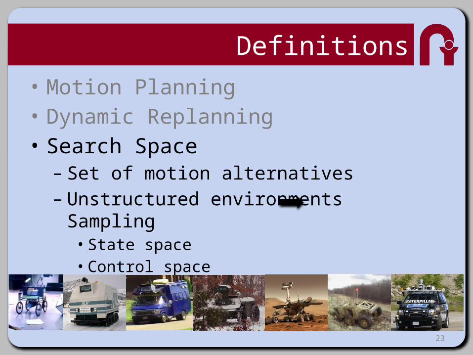
Definitions• Motion Planning• Dynamic Replanning• Search Space– Set of motion alternatives– Unstructured environments Sampling• State space• Control space

24

Definitions• Motion Planning• Dynamic Replanning• Search Space• Deterministic sampling– Fixed pattern, predictable– “Curse of dimensionality”

25

Definitions• Search space design– Input: robot properties– Output: state, control sampling– Maximize planner qualities (F, O, R, C)

• Design principle– Sampling rule

26

Outline

• Introduction• Deterministic Planning

– Hierarchical– Path Smoothing– Control Sampling– State Sampling

• Randomized Planning– PRMs– RRTs

• Derandomized Planners• Some applications

27

Local/Global

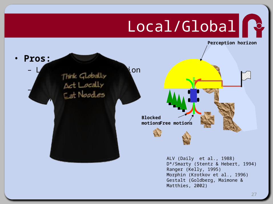
• Pros:– Local motion evaluation is fast – In sparse obstacles, works very well

Blocked motionsFree motions

Perception horizon

ALV (Daily et al., 1988)D*/Smarty (Stentz & Hebert, 1994)Ranger (Kelly, 1995)Morphin (Krotkov et al., 1996)Gestalt (Goldberg, Maimone & Matthies, 2002)

28

Local/Global


• Cons:– Search space differences


29

Local/Global




30

Local/Global




31

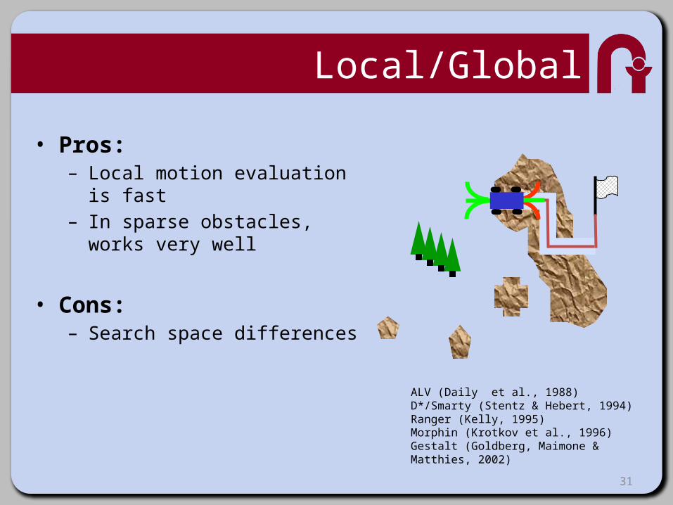
Local/Global




32

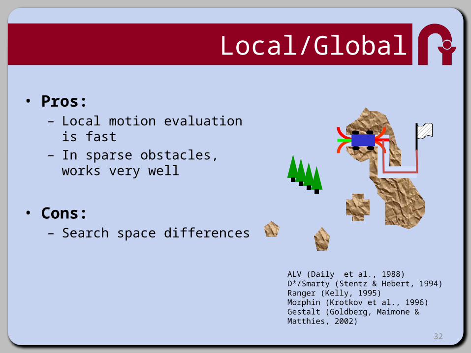
Local/Global




33

Local/Global




34

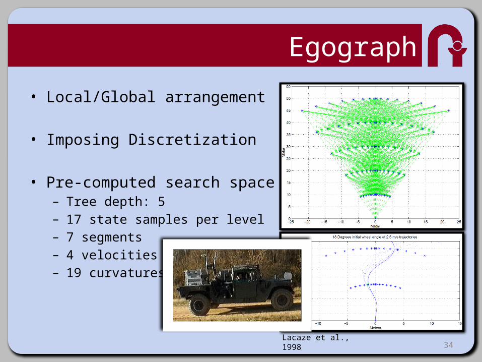
Egograph

• Local/Global arrangement

• Imposing Discretization

• Pre-computed search space– Tree depth: 5– 17 state samples per level– 7 segments– 4 velocities– 19 curvatures

Lacaze et al., 1998

35

Outline





36

Path Post-Processing

Lamiraux et al., 2002

Laumond, Jacobs, Taix, Murray, 1994

Khatib, Jaouni, Chatila, Laumond, 1997

37

Topological Property

38

Outline





39

Control Space Sampling

Barraquand & Latombe, 1993Lindemann & LaValle, 2006Kammel et al., 2008

Barraquand & Latombe:- 3 arcs (+ reverse) at max

- Discontinuous curvature- Cost = number of reversals- Dijkstra’s search

40

Robot-Fixed Search Space• Moves with the robot

• Dense sampling– Position

• Symmetric sampling– Heading– Velocity– Steering angle– …

• Tree depth– 1: Local (arcs) + Global (D*) (Stentz & Hebert, 1994)– 5: Egograph (Lacaze et al., 1998)– ∞: Barraquand & Latombe (1993)

40

41

Outline





42

World-Fixed Search Space

• Fixed to the world

• Dense sampling– (none)

• Symmetric sampling– Position– Heading– Velocity– Steering angle– …

• Dependency– Boundary value problem

Pivtoraiko & Kelly, 2005

Examples of BVP solvers:- Dubins, 1957- Reeds & Shepp, 1990- Lamiraux & Laumond, 2001- Kelly & Nagy, 2002- Pancanti et al., 2004- Kelly & Howard, 2005

43

Robot-Fixed vs. World-Fixed

Barraquand & Latombe

CONTROL

STATE CONTROL

STATE

State Lattice

44

State Lattice Benefits• State Lattice– Regularity in state sampling– Position invariance


45

Path Swaths


• State Lattice– Regularity– Position invariance

• Benefits– Pre-computing path swaths

46

World Fixed State Lattice

HLUT

Pivtoraiko & Kelly, 2005Knepper & Kelly, 2006


• Benefits– Pre-computing path swaths– Pre-computing heuristics


47

?


• Benefits– Pre-computing path swaths– Pre-computing heuristics– Dynamic replanning

48



• Benefits– Pre-computing path swaths– Pre-computing heuristics– Dynamic replanning

49

Nonholonomic D*

Expanded States

Motion Plan

Perception Horizon

Graphics: Thomas Howard

50

Nonholonomic D*

Pivtoraiko & Kelly, 2007Graphics: Thomas Howard

51

Boss

• “Parking lot” planner

• Regular 4D state sampling

• Pre-computed search space– Depth: unlimited– Multi-resolution– 32 (16) headings– 2 velocities– No curvature

LIkhachev et al., 2008

52



• Benefits– Pre-computing path swaths– Pre-computing heuristics– Dynamic replanning– Dynamic search space G0

G1

G3

G4G5

Search graph G0 G1 … Gn


53

Dynamic Search Space

Pivtoraiko & Kelly, 2008Graphics: Thomas Howard

54

Dynamic Search Space

55


START

GOAL• State Lattice– Regularity– Position invariance

• Benefits– Pre-computing path swaths– Pre-computing heuristics– Dynamic replanning– Dynamic search space– Parallelized search


56


START

GOAL


57

START

GOAL



0 0.02 0.04 0.06 0.08 0.1 0.120

2

4

6

8

10

12

14

16

epsilon

tree

size

ratio

58

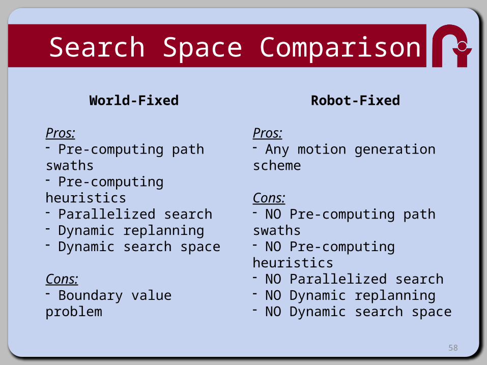
Search Space Comparison

Robot-Fixed

Pros:- Any motion generation scheme

Cons:- NO Pre-computing path swaths- NO Pre-computing heuristics- NO Parallelized search- NO Dynamic replanning- NO Dynamic search space

World-Fixed

Pros:- Pre-computing path swaths- Pre-computing heuristics- Parallelized search- Dynamic replanning- Dynamic search space

Cons:- Boundary value problem

59

Outline





60

A Few Randomized Planners

• Probabilistic Roadmaps (PRM)– Kavraki, Svestka, Latombe & Overmars, 1996

• Expansive Space Tree (EST)– Hsu, Kindel, Latombe & Rock, 2001

• Rapidly-Exploring Random Tree (RRT)– LaValle & Kuffner, 2001

• R* Search– Likhachev & Stentz, 2008

LaValle & Kuffner, 2001

61

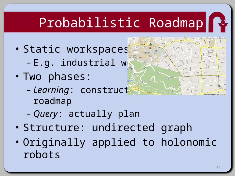
Probabilistic Roadmap

• Static workspaces– E.g. industrial workcells

• Two phases:– Learning: construct the

roadmap– Query: actually plan

• Structure: undirected graph• Originally applied to holonomic robots

62

Learning Phase

• Two steps:– Construction• Constructs edges and vertices to cover free C-space

uniformly

– Expansion• Tries to detect “difficult” regions and samples them

more densely

63

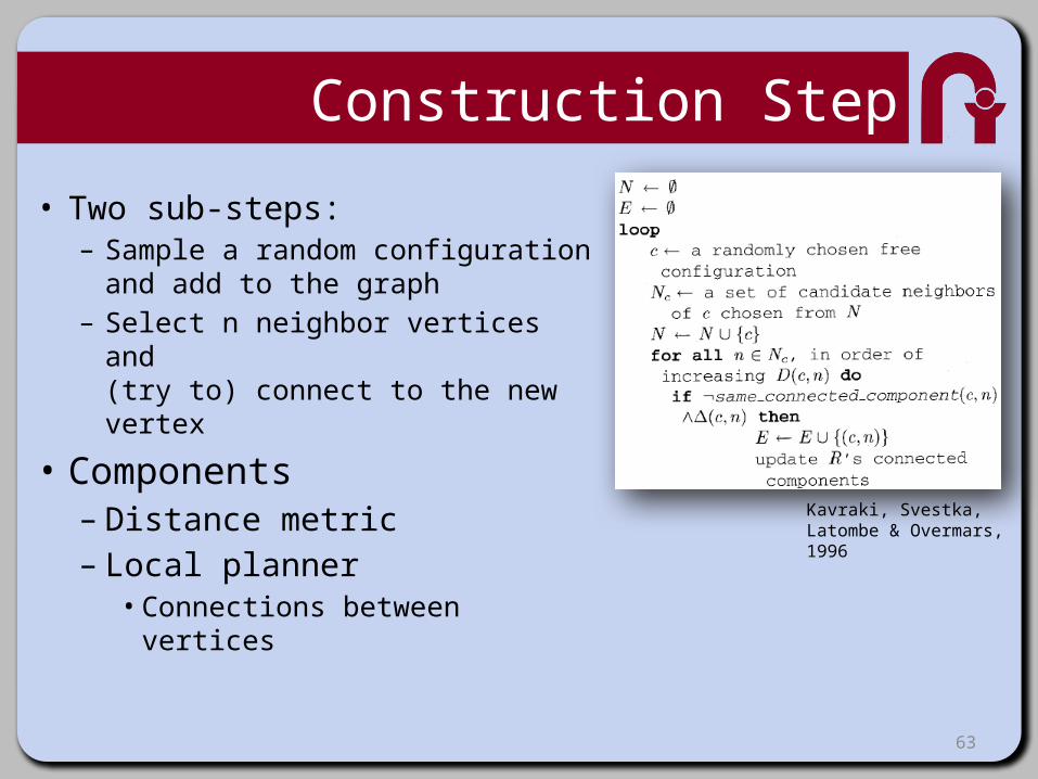
Construction Step

• Two sub-steps:– Sample a random configuration

and add to the graph– Select n neighbor vertices and

(try to) connect to the new vertex

• Components– Distance metric– Local planner• Connections between vertices

Kavraki, Svestka, Latombe & Overmars, 1996

64

Query Phase

• Graph is constructed• Apply any shortest-path

graph search • Smoothing:– Find “shortcuts”– Local planner is reused

Kavraki, Svestka, Latombe & Overmars, 1996

65

Outline





Original RRT

• Rapidly-Exploring Random Tree• Proposed for kino-dynamic planning

– Holonomic randomized planners existed before– Proposed to meet the need for randomized planners under

differential constraints

• Today, a work-horse for randomized search– Probabilistically complete– No optimality guarantees– Avoids “curse of dimensionality”

RRT in a Nutshell

• Given a tree (initially only x_{init})• Pick a sample, x, in state space, X

– Randomly– Sample uniform distribution over X

• Find nearest neighbor tree node, x_{near}, to x• Find a control that approaches x_{near}

– Unless you solve the BVP problem, won’t approach exactly

– Just do your best; you’ll arrive at x_{new} near to x

• Add x_{new} and the edge (x_{near}, x_{new}) to the tree

• Repeat

RRT Origins

• Khatib, IJRR 5(1), 1986– Potential fields for obstacle avoidance, mobile robots and manipulators

• Barraquand & Latombe, IJRR 10(6), 1993– Builds and searches a graph connecting local minima of a potential field– Monte-Carlo technique to escape local minima via Brownian motions

• Kavraki, Svestka, Latombe & Overmars, Transactions 12(4), 1996– Probabilistic roadmaps– Randomly generate a graph in a configuration space– Multi-query method, best for fixed manipulators

• Hsu, Latombe & Motwani, Int. J. of Comput. Geometry & App., 1997– Expansive Space Tree (EST), single-query method– Choose tree node to extend via biased probability measure– Apply random control– Collision checking in state*time space

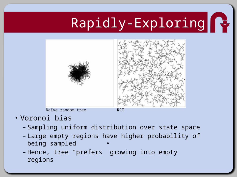
Rapidly-Exploring

• Voronoi bias– Sampling uniform distribution over state space– Large empty regions have higher probability of being

sampled– Hence, tree “prefers” growing into empty regions

Naïve random tree RRT

Voronoi Bias

Analysis

• Convergence to solution– Probability of failure (to find solution)

decreases exponentially with the number of iterations

• Probabilistic completeness

Examples

Quick overview of CBiRRT

• Constrained Bi-directional RRT

• Start with “unconstrained” RRT• Assume some constraints, e.g.:

– End-effector pose– Torque

• For each sample, x_{rand}, in X– Get x_{new} by tweaking x_{rand} until

constraints satisfied– … via optimization (gradient descent)– In text, “project sample onto constraint

manifold”

Growing the Tree

• Extending tree toward random sample– The sample is q_{target}– Nearest neighbor: q_{near}

• Step from q_{near} to q_{target}– In state space– Project each step onto constraint

manifold– Until you reach q_{target}’s

projection– Return, if can’t continue, e.g.

• Obstacles• Can’t project

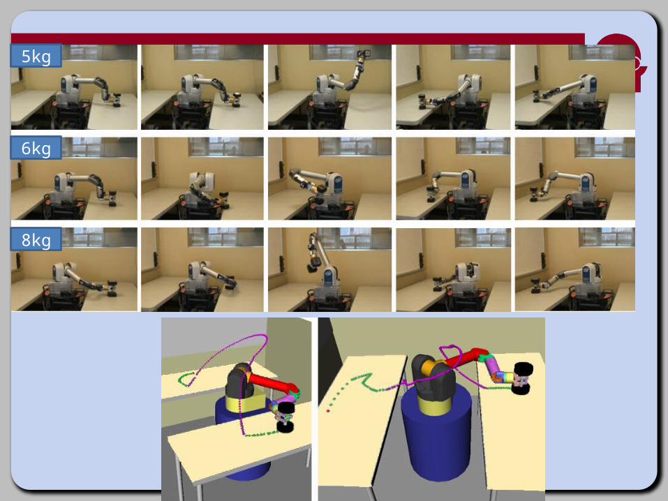
Results5kg

6kg

8kg

76

Outline




• Derandomized Planners• Some Applications

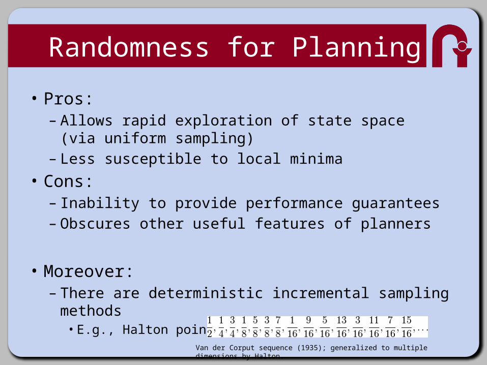
Randomness for Planning

• Pros:– Allows rapid exploration of state space

(via uniform sampling)– Less susceptible to local minima

• Cons:– Inability to provide performance guarantees– Obscures other useful features of planners

• Moreover:– There are deterministic incremental sampling methods

• E.g., Halton points Van der Corput sequence (1935); generalized to multiple dimensions by Halton.

Derandomized RRT

• Let’s implement Voronoi bias explicitly– Given tree– Compute Voronoi diagram wrt its nodes– Pick the sample to extend toward:

• Centroid of largest Voronoi region, or• Otherwise reduce size of largest empty ball

• Problem:– Voronoi diagram in arbitrary dimensions

– prohibitively expensive

Semi-Deterministic RRT

• So let’s go for a middle ground• Instead of a single x_{rand}• Draw a set k samples• Multi-Sample RRT (MS-RRT)

– Sort tree nodes acc. to:• how many samples they’re nearest neighbor for

– Pick node that “collected” most neighbors– Grow tree towards average of the neighbor samples

• It’s an estimate of the Voronoi centroid• As k∞, we get exact Voronoi centroid

• “… I shall call him MS-RRTa!”

Now, a Deterministic RRT

• … but with approximate Voronoi bias• Recall: picking k points– Instead of randomly,– Use k uniformly distributed, incremental

deterministic samples– E.g., Halton points

• The rest stays essentially the same

• Meet MS-RRTb!

Results

• Local minima– Both MS-RRT are more greedily Voronoi-biased– Local minima issues – more pronounced than RRT– Paper’s workaround:

• Introduce obstacle nodes in tree• It’s the nodes that land in obstacles• A mechanism “to remember” not to grow the tree there any more

• Sensitivity to metrics– Increased for MS-RRTa,b, – Since Voronoi depends on metric

• Nearest-neighbor computation– More expensive than O(log n)– Increased demand for it in MS-RRTa,b

Results

83

Outline





84

Mobile Manipulation• Arbitrary mobility constraints• Optimal solution– Up to representation

• Parallelized computation• Automatically designed

85

Dynamics Planning

86

Summary• Deterministic planning– Hierarchical– Path Smoothing– Control Sampling– State Sampling

• Randomized planning• PRMs• RRTs

mihail pivtoraiko 1. motion planning the challenge: reliable autonomous robots 2 navlab, 1985 boss,...

Documents

plan local slide

local global alv

local global structure

d global planners

dynamics planning

corridor global planner

local mo

deterministic planners