michele segata and renato lo cigno -...
TRANSCRIPT

DISI - Via Sommarive, 14 - 38123 POVO, Trento - Italyhttp://disi.unitn.it
Models and Performance of VANET basedEmergency Braking
Michele Segata and Renato Lo Cigno
March 2011
Technical Report # DISI-11-354Version 0.1


Extended Abstract
The network research community is working in the field of automotive to pro-vide VANET based safety applications to reduce the number of accidents, deaths,injuries and loss of money. Several approaches are proposed and investigatedin VANET literature, but in a completely network-oriented fashion. Most of themdo not take into account application requirements and no one considers the dy-namics of the vehicles. Moreover, message repropagation schemes are widelyproposed without investigating their benefits and using very complicated ap-proaches.
This technical report, which is derived from the Master Thesis of MicheleSegata, focuses on the Emergency Electronic Brake Lights (EEBL) safety appli-cation, meant to send warning messages in the case of an emergency brake, inparticular performing a joint analysis of network requirements and provided ap-plication level benefits. The EEBL application is integrated within a CollaborativeAdaptive Cruise Control (CACC) which uses network-provided information to au-tomatically brake the car if the driver does not react to the warning. Moreover,an information aggregation scheme is proposed to analyze the benefits of reprop-agation together with the consequent increase of network load. This protocolis compared to a protocol without repropagation and to a rebroadcast protocolfound in the literature (namely the weighted p-persistent rebroadcast).
The scenario is a highway stretch in which a platoon of vehicles brake down toa complete stop. Simulations are performed using the NS-3 network simulationin which two mobility models have been embedded. The first one, which is calledIntelligent Driver Model (IDM) emulates, the behavior of a driver trying to reacha desired speed and braking when approaching vehicles in front. The second one(Minimizing Overall Braking Induced by Lane change (MOBIL)) instead, decideswhen a vehicle has to change lane in order to perform an overtake or optimize itspath. The original simulator has been modified by
• introducing real physical limits to naturally reproduce real crashes;
• implementing a CACC;
• implementing the driver reaction when a warning is received;
• implementing different network protocols.

The tests are performed in different situations, such as different number oflanes (one to five), different average speeds, different network protocols and dif-ferent market penetration rates and they show that:
• the adoption of this technology considerably decreases car accidents sincethe overall average maximum deceleration is reduced;
• network load depends on application-level details, such as the implementa-tion of the CACC;
• VANET safety application can improve safety even with a partial market pen-etration rate;
• message repropagation is important to reduce the risk of accidents whennot all vehicles are equipped;
• benefits are gained not only by equipped vehicles but also by unequippedones.
Keywords: VANET; Vehicular Networks; Emergency Braking Control; Cruise Con-trol; NS-3 simulation; re-broadcast schemes.

UNIVERSITÀ DEGLI STUDI DI TRENTOFacoltà di Scienze Matematiche, Fisiche e Naturali
UNIVERSITY OF TRENTO - Italy
Corso di Laurea Magistrale in Informatica
Final Thesis
Models and performance of VANETbased emergency braking
Relatore/1st Reader: Laureando/Graduant:Prof. Renato Antonio Lo Cigno Michele Segata
Anno Accademico 2009 - 2010


C O N T E N T S
LIST OF FIGURES ix
LIST OF TABLES xi
1 INTRODUCTION 1
1.1 The idea of VANET . . . . . . . . . . . . . . . . . . . . . . . . . . . . . 2
1.2 Emergency Electronic Brake Lights . . . . . . . . . . . . . . . . . . . . 3
2 COMMUNICATION TECHNOLOGIES 7
2.1 802.11 basics . . . . . . . . . . . . . . . . . . . . . . . . . . . . . . . . . 7
2.1.1 802.11e and QoS . . . . . . . . . . . . . . . . . . . . . . . . . . 11
2.2 802.11p . . . . . . . . . . . . . . . . . . . . . . . . . . . . . . . . . . . . 13
2.3 Applications and open issues . . . . . . . . . . . . . . . . . . . . . . . 14
2.3.1 Theoretical computation of network load . . . . . . . . . . . . 17
3 RELATED WORK 19
4 MOBILITY MODELS AND SIMULATIONS 29
4.1 NS-3 and the mobility simulator . . . . . . . . . . . . . . . . . . . . . 30
4.2 Intelligent Driver Model . . . . . . . . . . . . . . . . . . . . . . . . . . 31
4.3 MOBIL lane change model . . . . . . . . . . . . . . . . . . . . . . . . . 36
4.4 Changes in the mobility simulator . . . . . . . . . . . . . . . . . . . . 39
4.4.1 Crash simulation and management . . . . . . . . . . . . . . . 39
4.4.2 Accelerometer and imperfect clock . . . . . . . . . . . . . . . . 39
4.4.3 CACC . . . . . . . . . . . . . . . . . . . . . . . . . . . . . . . . 40
4.4.4 Air resistance induced deceleration . . . . . . . . . . . . . . . 41
4.5 Network protocols . . . . . . . . . . . . . . . . . . . . . . . . . . . . . 42
5 PERFORMED TESTS 47
5.1 Simulation parameters . . . . . . . . . . . . . . . . . . . . . . . . . . . 48
5.2 Single lane tests . . . . . . . . . . . . . . . . . . . . . . . . . . . . . . . 50
5.3 Multi lane tests . . . . . . . . . . . . . . . . . . . . . . . . . . . . . . . 59
5.4 Single lane market penetration rate tests . . . . . . . . . . . . . . . . . 66
5.5 Multi lane market penetration rate tests . . . . . . . . . . . . . . . . . 68
6 FUTURE WORK 71
vii

viii Contents
7 CONCLUSIONS 73
BIBLIOGRAPHY 75
LIST OF ACRONYMS 81

L I S T O F F I G U R E S
Figure 1.1 The Post-crash warning application . . . . . . . . . . . . . . . . 2
Figure 1.2 Brake lights visibility problem . . . . . . . . . . . . . . . . . . 3
Figure 2.1 DSSS modulation . . . . . . . . . . . . . . . . . . . . . . . . . . 8
Figure 2.2 OFDM subcarriers representation . . . . . . . . . . . . . . . . . 9
Figure 2.3 The 802.11 DCF access mechanism . . . . . . . . . . . . . . . . 11
Figure 2.4 AC prioritization through AIFS . . . . . . . . . . . . . . . . . . 13
Figure 2.5 Shadowing problem . . . . . . . . . . . . . . . . . . . . . . . . 15
Figure 2.6 Fading problem . . . . . . . . . . . . . . . . . . . . . . . . . . . 15
Figure 2.7 EEBL congestion issue . . . . . . . . . . . . . . . . . . . . . . . 16
Figure 3.1 Different persistence mechanisms [28]. . . . . . . . . . . . . . 20
Figure 3.2 Different neighborhood conditions pointed out in the DV-
CAST paper . . . . . . . . . . . . . . . . . . . . . . . . . . . . . . 23
Figure 3.3 The clustering scheme of the TrafficGather protocol definedby Chang et al. [37]. . . . . . . . . . . . . . . . . . . . . . . . . 24
Figure 4.1 Structure of the simulator . . . . . . . . . . . . . . . . . . . . . 32
Figure 4.2 Plot of the αfree term of the IDM model . . . . . . . . . . . . . 33
Figure 4.3 Graphical representation of the αint term in the case of ahigh approach rate for different values of b . . . . . . . . . . . 35
Figure 4.4 The MOBIL lane change model . . . . . . . . . . . . . . . . . . 38
Figure 5.1 Trace of the accelerations in time for pure idm test, 41.66 m/s 51
Figure 5.2 Trace of the accelerations in time of the first five vehicles forthe limited idm test . . . . . . . . . . . . . . . . . . . . . . . . 51
Figure 5.3 Quantification of the benefits of an EEBL system, for a 100%market penetration rate . . . . . . . . . . . . . . . . . . . . . . 52
Figure 5.4 Traces of decelerations for different experiments . . . . . . . . 54
Figure 5.5 Contention for the channel . . . . . . . . . . . . . . . . . . . . 55
Figure 5.6 Network load for eebl experiment, one lane 36.11 m/s . . . . 58
Figure 5.7 Network load for eeblr and eebla experiments, one lane36.11 m/s . . . . . . . . . . . . . . . . . . . . . . . . . . . . . . 58
Figure 5.8 Natural doubling of network load due to message repropa-gation . . . . . . . . . . . . . . . . . . . . . . . . . . . . . . . . . 59
Figure 5.9 CDFs of maximum loads of all single-lane experiments, foraverage speed 36.11 m/s . . . . . . . . . . . . . . . . . . . . . . 60
ix

x List of Figures
Figure 5.10 Average loads for test with five lanes, average speed 36.11
m/s . . . . . . . . . . . . . . . . . . . . . . . . . . . . . . . . . . 62
Figure 5.11 Collision detection problem . . . . . . . . . . . . . . . . . . . . 63
Figure 5.12 Percentage of packets that have been sent but not receivedby any node . . . . . . . . . . . . . . . . . . . . . . . . . . . . . 63
Figure 5.13 Average number of offered packets during the simulationfor the different protocols . . . . . . . . . . . . . . . . . . . . . 64
Figure 5.14 CDFs of maximum loads of all five-lane experiments, for av-erage speed 36.11 m/s . . . . . . . . . . . . . . . . . . . . . . . 65
Figure 5.15 Percentage of cars involved in accidents for single-lane mar-ket penetration rate tests . . . . . . . . . . . . . . . . . . . . . . 66
Figure 5.16 Percentage of cars crashed divided for equipped and un-equipped for the single-lane test . . . . . . . . . . . . . . . . . 67
Figure 5.17 Percentage of cars involved in accidents for multi-lane mar-ket penetration rate tests, average speed 36.11 m/s . . . . . . 69
Figure 5.18 Higher probability of “natural” propagation for a multi-lanehighway . . . . . . . . . . . . . . . . . . . . . . . . . . . . . . . 70
Figure 5.19 Percentage of cars crashed divided for equipped and un-equipped for the five lanes test, average speed 36.11 m/s . . 70

L I S T O F TA B L E S
Table 2.1 CWs size calculation in 802.11e . . . . . . . . . . . . . . . . . . 12
Table 2.2 CWs size for 802.11e on 802.11a PHY . . . . . . . . . . . . . . . 12
Table 2.3 AIFS values for 802.11e defined in IEEE 802.11e [17] . . . . . . 13
Table 2.4 MAC parameters for 802.11p CCH . . . . . . . . . . . . . . . . . 14
Table 2.5 MAC parameters for 802.11p SCH . . . . . . . . . . . . . . . . . 14
Table 2.6 802.11p CCH PHY and MAC parameters for the AC with high-est priority (AC_VO) . . . . . . . . . . . . . . . . . . . . . . . . . 18
Table 4.1 Required message data set for EEBL application, as sug-gested by U.S. DOT [6] . . . . . . . . . . . . . . . . . . . . . . . 44
Table 4.2 Additional header for beacons and EEBL packets . . . . . . . . 44
Table 5.1 IDM parameters used in simulations . . . . . . . . . . . . . . . 49
Table 5.2 MOBIL parameters used in simulations . . . . . . . . . . . . . . 49
Table 5.3 Network parameters . . . . . . . . . . . . . . . . . . . . . . . . 50
xi


1 I N T R O D U C T I O N
Vehicles are a fundamental part of our life. We use them every day for differentpurposes, from work to fun. As written in the National Transportation Statisticspublished by the U.S. Department of Transportation [1], the number of cars inthe United States in year 2008 was around 137 million, without including motor-cycles, trucks and buses. If we consider that the number of inhabitants of theU.S.A. is around 300 million, including non driving people such as infants, wecan understand how much road transportation is diffused. In Italy, the numberof cars at the beginning of 2010 was 36 million [2], for a population of 60 millionpeople [3] (60 cars every 100 persons).
Safety is one of the most important concerns: according to the FARS/GES 2008Data Summary [4], in 2008 there were 5.8 million crashes in the United States.Roughly 34.000 were fatal, 1.6 million have caused people injuries while the oth-ers have caused only property damages. In 2000
1 the economic impact of caraccidents was $230.6 billion [5], which means roughly $820 per living person(still in the U.S.). These values includes costs related to lost productivity, medi-cal costs, legal and court costs, emergency service costs, insurance administrationcosts, travel delay, property damage and workplace losses.
These numbers show how much it is important to work on accident prevention:first of all to reduce deaths and injuries, second to save money and finally to savepeople time. Indeed when a car crash happens, people can remain stuck in atraffic jam for a long time.
Vehicle-related technologies are giving a great help in security improvementand driving comfort. For security, think of the Antilock Braking System (ABS),which prevents wheel lock in violent braking, or the Electronic Stability Control(ESC), which improves stability by detecting and minimizing skids. For comfort,think of parking sensors or GPS based navigation systems.
1 At time of writing this was the most recent report available
1

2 INTRODUCTION
1.1 THE IDEA OF VANET
In the field of Computer Science and Networking, researchers are actively work-ing to develop WLAN enabled communications between vehicles. This kind of net-works has been defined as VANETs, which stands for Vehicular Ad-hoc NETworks:this acronym is inspired by Mobile Ad-hoc NETwork (MANET). A MANET is a kindof network where the position of the nodes is not fixed and they do not rely on apreexisting infrastructure, so every communicating device actively partecipate inrouting and data forwarding.
Indeed a vehicular network can be considered as a particular kind of MANET,but with some differences. VANET nodes do not move randomly but in an orga-nized fashion, and their movements are constrained in streets.
Inter-vehicle communications give the basis for any kind of networking soft-ware. The Vehicle Safety Communications Project [6] identifies a set of applicationsclassified into safety and non-safety, but always related to the pure automotivefield.
An example of a safety application described in the document is the Post-crashwarning: the idea is broadcasting of warning messages by cars that are stuck ona lane due to an accident or a mechanical breakdown. Vehicles receiving thesewarnings will inform their drivers of the danger, to avoid potential collisions. Itcan be very useful, for example, when the driver of the crashed vehicle has notyet placed the red warning triangle on the road, or in the case of limited visibilitydue to fog. Look for an example at Figure 1.1. Classified as non-safety is insteadthe Instant messaging application, which enables drivers to send text messageseach other, for example to signal problems such as a flat tire. Another exampleis the Enhanced Route Guidance and Navigation (ERGN) which can inform theGPS-based navigation system of recent road changes, such as detours, by meansof messages received from access points placed on the side of the road.
Lane 1
Lane 2
Lane 3
CRASH CRASH CRASH CRASH
Figure 1.1: The Post-crash warning application. Crashed vehicle signals the danger usingwireless messages and incoming vehicles can be warned quickly even in lowvisibility conditions
1.2 EMERGENCY ELECTRONIC BRAKE LIGHTS 3
These are only three examples out of tens described in U.S. DOT [6]. As saidbefore these are pure automotive applications, while others can also be supportedby VANETs. For example they can provide Internet connection or inter-vehiclegaming as a novel way of entertainment.
Different applications have clearly different requirements, in terms of band-width, connection duration, delay, etc. . . and it is not possible to analyze them allin a single thesis. The next section will introduce the aim of this work.
1.2 EMERGENCY ELECTRONIC BRAKE LIGHTS
This thesis will focus on a safety application, in particular on the EmergencyElectronic Brake Lights (EEBL).
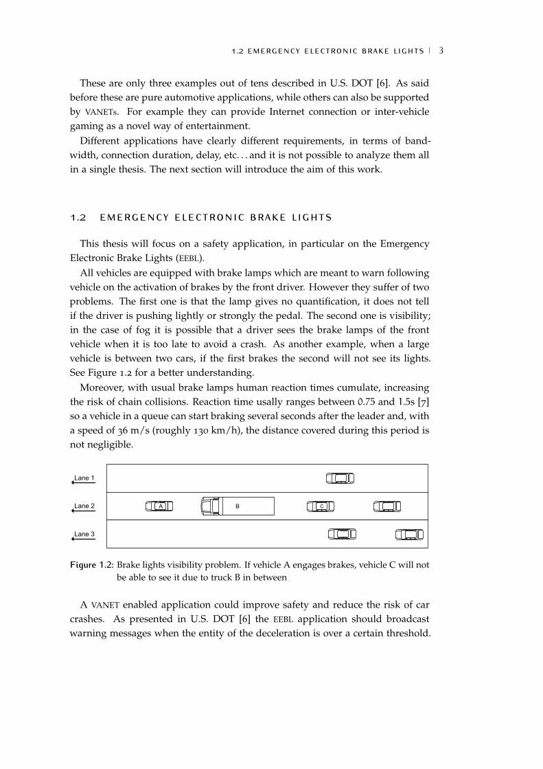
All vehicles are equipped with brake lamps which are meant to warn followingvehicle on the activation of brakes by the front driver. However they suffer of twoproblems. The first one is that the lamp gives no quantification, it does not tellif the driver is pushing lightly or strongly the pedal. The second one is visibility;in the case of fog it is possible that a driver sees the brake lamps of the frontvehicle when it is too late to avoid a crash. As another example, when a largevehicle is between two cars, if the first brakes the second will not see its lights.See Figure 1.2 for a better understanding.
Moreover, with usual brake lamps human reaction times cumulate, increasingthe risk of chain collisions. Reaction time usally ranges between 0.75 and 1.5s [7]so a vehicle in a queue can start braking several seconds after the leader and, witha speed of 36 m/s (roughly 130 km/h), the distance covered during this period isnot negligible.
Lane 1
Lane 2
Lane 3
C A B
Figure 1.2: Brake lights visibility problem. If vehicle A engages brakes, vehicle C will notbe able to see it due to truck B in between
A VANET enabled application could improve safety and reduce the risk of carcrashes. As presented in U.S. DOT [6] the EEBL application should broadcastwarning messages when the entity of the deceleration is over a certain threshold.

4 INTRODUCTION
These messages should provide information about the braking vehicle, such asspeed, acceleration, position, etc. . . In this way both problems of quantificationand visibility will be solved; a driver could be informed that, five vehicles infront, a car is braking with a deceleration of, for example, 3 m/s2 and be morefocused on driving.
However, the most interesting application is that EEBL-provided informationcould be passed to an Adaptive Cruise Control (ACC) system. A Cruise Control(CC) is a system which mantains a vehicle on a constant speed selected by thedriver. The Adaptive Cruise Control improves the behavior of the CC by automat-ically decreasing speed if the vehicle is too close to the front one and by maintaingthe safety distance. The ACC works using a radar which detects if there is a vehiclein front and determines its speed and distance.
Unfortunately, radar based ACC can give information only about the front ve-hicle, while a driver could be interested in having a wider perspective, not onlyabout vehicles in the same lane but also in other lanes. Indeed if a car appliesthe brakes strongly, knowing it is useful for all drivers behind: as an example,imagine the situation in which an animal crosses the street.
Instead of using a radar, the ACC could work using the EEBL messages receivedfrom other vehicles: the ones from front car to mantaing safety distance and applythe brakes if needed, the others to give a global perspective to the driver. Thiswill be the concept in this thesis, but in reality this information could be used toimprove traffic flow by using the so called Collaborative Adaptive Cruise Control(CACC). The CACC is an improved version of the ACC which uses the informationof more vehicles in front to mantain a lower inter-vehicle distance, increasing flowdensity without a higher risk of crashes, since variations are obtained in real timevia wireless messages. More details about the advantages of CACC can be foundin van Arem et al. [8].
In this thesis the CACC will be considered as a system which only mantainssafety distance and brakes the car in the case of an emergency situation; it willnot implement a car following mechanism, so it will not keep a constant distancefrom front vehicle. If the driver decides to go slower than front vehicle, the systemwill not accelerate.
An advantage of VANET technology is that once a WLAN card with a process-ing unit has been installed, all the applications which do not require to activelycontrol the vehicle (e.g., the Post-Crash warning) would be simply treated as YetAnother VANET Application and could be installed, for example, via a software up-date.

1.2 EMERGENCY ELECTRONIC BRAKE LIGHTS 5
Obviously some issues have to be considered. VANETs rely on wireless commu-nications so most of the problems (if not more) that we encounter in WLANs willhave to be faced.
The focus of this thesis will be a joint analysis of EEBL application and networkprotocols: indeed as described in Chapter 3 this approach is completely missingin the literature. Either the research completely focuses on network performancesor only describes the advantages of a particular application. Second an analysis ofthe benefits of message repropagation will be performed: is it worth it to replicateEEBL messages more far than a single hop? If so, which consequences has this onthe network? Finally, the thesis will analyze the effectiveness of a simple messageaggregation protocol.


2 C O M M U N I C AT I O N T E C H N O LO G I E S
The Federal Communications Commission (FCC) in 1999 has begun the pro-cess of standardization for vehicular communications by allocating the 5.850-5.925
GHz band (75 MHz) for Dedicated Short Range Communications (DSRC)1. Thena set of protocols for Wireless Access in Vehicular Environments (WAVE) has beendeveloped by IEEE, in particular by the working groups 802.11p [9] and P1609
[10, 11, 12, 13].
P1609 (P1609.1 to P1609.4) focuses on higher layers: for example P1609.2 ad-dresses security issues, such as encryption and authentication, while P1609.4 re-gards multi-channel operations. Given the aims of this thesis, these protocols willnot be described in details.
802.11p is instead an amendment to IEEE 802.11 [14] which defines the changesfor PHY and MAC layer to address communication requirements for vehicular net-works, not only Vehicle-to-Vehicle (V2V) but also Vehicle-to-Roadside (V2R) (andviceversa). Indeed some VANET applications cannot work in a pure V2V network,because interaction with the “outside world” is needed. Think as an example tothe ERGN application mentioned in Section 1.1: for GPS maps update an accesspoint on the road is needed, at least for initial diffusion. This access point in theVANET terminology is called RoadSide Unit (RSU).
Notice that none of this standards defines application level protocols like re-broadcast metodology or aggregation mechanisms; this aspects are left to theresearch community.
Understanding 802.11p is fundamental because it has been employed in thesimulations described in Chapter 5, but first some notions about 802.11 have tobe given.
2.1 802.11 BASICS
The 802.11 standard specifies Physical Layer (PHY) and Medium Access Control(MAC) for WLANs, so it defines the characteristics of the lower layers, such as trans-
1 The FCC news release can be found at http://www.fcc.gov/Bureaus/Engineering_Technology/
News_Releases/1999/nret9006.html
7

8 COMMUNICATION TECHNOLOGIES
mission speeds, transmission techniques, frames format, medium access mecha-nisms, etc . . . .
Commonly used 802.11 protocols work in the Industrial Scientific and Medical(ISM) band, in particular in the 2.4 GHz (802.11 b and g) and the 5 GHz (802.11a)bands. They use different modulation mechanisms, providing different transmis-sion speeds. For example, 802.11b uses Direct Sequence Spread Spectrum (DSSS)with a maximum transmission speed of 11 Mbps. 802.11a and g instead useOrthogonal Frequency Division Multiplexing (OFDM) which provides up to 54
Mbps.The DSSS technique is represented (in a very simplified way) in Figure 2.1: ba-
sically a random sequence of 1 and -1 values (called chipping sequence) is gen-erated at a frequency much more higher than the one of the original signal. Theproduct of the signal and the sequence results in the spreading of the energy overa wider range of frequencies. The receiver can perform the “de-spreading” bymultiplying received signal by the same chipping sequence used by the sender,so the synchronization between sender and received is required for a correct de-coding.
The advantage of the DSSS modulation is the resistance to narrow-band inter-ference. Imagine that the original signal in Figure 2.1 is the interference: whenthe receiver applies the chipping sequence to received signal, the interference isspreaded over the spectrum, so the original signal can be decoded anyhow.
Figure 2.1: DSSS modulation
OFDM uses instead a set of orthogonal subcarriers (Figure 2.2) to perform mul-tiplexing of datastreams. In other words, datastreams are sent in parallel, each

2.1 802.11 BASICS 9
of them modulated with a different subcarrier: this mechanism permits to reachhigher transmission speeds.
Two signals ϕn(t) and ϕm(t) are said to be orthogonal in the interval a < t < bif
∫ba
ϕn(t)ϕ∗m(t)dt = 0 [15]. (2.1)
In Equation (2.1), ϕ∗m(t) indicates the complex conjugate of ϕ∗m(t), that is thesame function but with the imaginary part negated. For example, the complexconjugate of 3 + 2i is 3 − 2i. The orthogonality of the subcarriers is importantbecause it ensures that no inter-carrier interference occurs during transmission.
Notice that DSSS and OFDM are complex modulation techniques, but their de-scription is beyond the scope of this thesis. Two comprehensive reading withbackground, algorithms, mathematical definitions and examples are the books byCouch [15] and Paulraj et al. [16].
Figure 2.2: OFDM subcarriers representation
All the 802.11 protocols, which are completely different by the point of viewof the physical layer, use the same mechanism to obtain access to the medium,that is the so called Distributed Coordination Function (DCF), which follows theCarries Sense Multiple Access with Collision Avoidance (CSMA/CA) protocol. Theprinciple of CSMA is to “listen” if the channel is busy before transmitting data,in order to avoid the disruption of ongoing transmissions. Collision avoidanceinstead refers to the procedure that the stations obey in order to contend forthe channel and minimize the number of collisions. A collision occurs when

10 COMMUNICATION TECHNOLOGIES
two nodes (or more) access the channel simultaneously, often causing trasmittedpackets to be lost2.
The DCF basically uses a random defer time (backoff, counted in slots) for trans-mission if the channel is sensed as busy: before performing the backoff, everystation must wait a predefined period of time. Figure 2.3 gives a graphical repre-sentation of the mechanism. The purpose of this amount of time is the prioriti-zation of possible subsequent transmissions. To clarify this aspect, it is better todescribe the time intervals of Figure 2.3:
SIFS the Short Inter Frame Space is the time elapsed between frames belongingto the same transmission, for example a frame and its acknowledgement.Indeed, for unicast messages, 802.11 uses an ACK, which is the only wayto determine if a packet has been correctly received. SIFS is the shortesttime because the ACK is the packet with higher priority after a transmission.Another example of usage of SIFS is when fragmentation is adopted: in thiscase the transmission will be a sequence of frames and ACKs separated bySIFS;
PIFS the PCF Inter Frame Space is used when polling is performed by the accesspoint. The access point can indeed give access to the channel to a particularstation in its polling list. This has priority over the distributed channelaccess, so PIFS is the shortest time after SIFS. It is computed as a SIFS plusone slot time;
DIFS after a Distributed Inter Frame Space, stations can begin the backoff pro-cedure and try to access the channel. It is computed as a SIFS plus twoslot times. This time is higher than SIFS and PIFS: if the stations “hear” thechannel free for this period of time no higher priority transmission will beperformed.
The backoff procedure is simply a “countdown” of a number of slots that israndomly generated in the range [0,CW], where CW is the Contention Window.While counting, a station continuously listens to the channel; if the countdownreaches 0, it can start transmitting, otherwise the value is saved and countdowncontinues at next contention. If two (or more) stations reach 0 at the same time,a collision occurs; the collision is detected by the missing ACK and, at next con-tention, stations will perform again the backoff procedure but with a doubled CW.This procedure is repeated until successfull transmission or until a maximum
2 This is not always true, for example when transmitting stations are very far. In this case the signalof one transmitter could be simply “heard” as non-disrupting noise by a receiver near to the othertransmitter

2.1 802.11 BASICS 11
number of attempts has been reached. After a successfull transmission the sizeof the CW is shrunken back to the minimum value (CWmin). On collision instead,the CW can grow up to a maximum value CWmax. For example, the values forCWmin and CWmax for 802.11b and g are 31 and 1023 slots respectively. Noticethat in the case of collision, the transmission of the packet is not stopped, becausethere is no way to detect it, as for CSMA/CD.
Busy medium SIFS
PIFS
DIFS
Backoff Frame
Slot
Figure 2.3: The 802.11 DCF access mechanism
In the case of broadcasting this procedure is much more simplified, becausemessages are directed to all stations in the transmission range of the sender andthe ACK cannot be used. If the receivers are twenty, then twenty acknowledge-ments should be sent, wasting resources. Moreover, what can sender do if noACK is received? Has a collision occured or are there no receivers in the transmis-sion range? A list of neighbors should be mantained, but then what happens if anode suddenly shuts down? The sender would keep re-sending the same packetwaiting for the ACK of the missing station which will never arrive.
So for broadcast messages, after packet transmission, a DIFS elapses and sta-tions start again the contention. Rebroadcast mechanisms should be developed athigher layers. Moreover due to the absence of acknowledgements, the CW nevergrows.
2.1.1 802.11e and QoS
In 2005 an amendment to the original 802.11 has been developed by the workinggroup e in order to support Quality of Service (QoS)[17]. The main enhancementis the replacement of the DCF with the Enhanced Distributed Channel AccessFunction (EDCAF), which introduces four access categories AC. The idea is to havefour queues for packets with different priorities and let them compete virtuallyfor channel access as with DCF: when two packets of different queues collide, theone with highest priority access the channel, while the other behaves as a realcollision has occured. The access categories are:
AC_BK the AC with lower priority, for background traffic;
AC_BE the second AC for best effort traffic;

12 COMMUNICATION TECHNOLOGIES
AC_VI the third AC for video;
AC_VO the AC with higher priority, for voice.
The internal contention mechanism is not enough because packets prioritiza-tion does not work among different stations. So different CWs has been used fordifferent access categories. Table 2.1 shows how the values of CWmin and CWmax
are computed in 802.11e. The table could seem a little bit misleading: the actualvalues of CWmin and CWmax must be computed depending on the physical layer.Indeed 802.11e describes only the EDCA mechanism, but this must be used on topof another 802.11 PHY standard, for example 802.11a. By looking at IEEE 802.11
[14, p. 626] it is possible to retrieve the values of CWmin and CWmax for 802.11aOFDM PHY (bandwidth 20 MHz), that are 15 and 1023 respectively. So if we use802.11e on top of 802.11a PHY, EDCA will use the values shown in Table 2.2.
AC CWmin CWmax
AC_BK CWmin CWmax
AC_BE CWmin CWmax
AC_VI (CWmin+1)/2 - 1 CWmin
AC_VO (CWmin+1)/4 - 1 (CWmin+1)/2 - 1
Table 2.1: CWs size calculation in 802.11e
AC CWmin CWmax
AC_BK 15 1023
AC_BE 15 1023
AC_VI 7 15
AC_VO 3 7
Table 2.2: CWs size for 802.11e on 802.11a PHY
As shown by Tinnirello et al. [18], the CW differentiation is not enough andmust be combined with the usage of different DIFS for different access categories.In particular a different Arbitration Inter Frame Space (AIFS) has been defined foreach AC. AIFS[i] is the number of slot after a SIFS that AC i must wait before tryingto access the channel. Low priority queues have higher AIFS value: Figure 2.4shows how AIFS is used in EDCA. Table 2.3 shows the values of AIFS for thedifferent access categories.

2.2 802.11P 13
Busy medium SIFS
PIFS
DIFS
Backoff Frame
Slot
AIFS[i]Backoff
BackoffAIFS[j]
Figure 2.4: AC prioritization through AIFS
AC AIFS
AC_BK 7
AC_BE 3
AC_VI 2
AC_VO 2
Table 2.3: AIFS values for 802.11e defined in IEEE 802.11e [17]
2.2 802.11P
The 802.11p standard [9] is a variant of 802.11a conceived for vehicular commu-nications. One of the most important features of 802.11p is the ability to commu-nicate in a complete ad-hoc manner, without the usage of the association processtypical of 802.11 based communications. The association phase indeed would lasttoo long for a highly mobile network as a VANET. So, as said before, securitymechanism must be handled at higher layer.
Regarding the physical layer, the main change from 802.11a is the channel spac-ing, which as been reduced from 20 MHz to 10 MHz (OFDM is used), supporting3, 4.5, 6, 9, 12, 18, 24 and 27 Mbps. The 10 MHz bandwidth is used due to robust-ness issues and the possibility to reuse existing wireless chipsets [19]. With thereduction of the channel spacing other PHY parameters change, such as slot timeand SIFS time3. The transmission range, according to U.S. DOT [6], should be upto 1 km.
Seven channels have been reserved, in particular one Control CHannel (CCH)and six Service CHannels (SCHs). The aims of the CCH are basically two. The firstone is sending safety messages between vehicles while the second is service adver-tisement: by using the CCH a vehicle can announce a service on a SCH. Since this
3 So consequently also DIFS

14 COMMUNICATION TECHNOLOGIES
thesis focuses on a safety application, only the CCH will be considered. Furtherdetails are given in the book by Hartenstein and Laberteaux [19].
Regarding the MAC layer instead, the EDCA mechanism of 802.11e is adoptedin order to give safety messages a higher priority w.r.t. non-safety messages.Table 2.4 and Table 2.5 show the EDCA parameters for CCH and SCH.
AC CWmin CWmax AIFS
AC_BK CWmin (15) CWmax (1023) 9
AC_BE (CWmin+1)/2 - 1 (7) CWmin (15) 6
AC_VI (CWmin+1)/4 - 1 (3) (CWmin+1)/2 - 1 (7) 3
AC_VO (CWmin+1)/4 - 1 (3) (CWmin+1)/2 - 1 (7) 2
Table 2.4: MAC parameters for 802.11p CCH
AC CWmin CWmax AIFS
AC_BK CWmin (15) CWmax (1023) 7
AC_BE CWmin (15) CWmax (1023) 3
AC_VI (CWmin+1)/2 - 1 (7) CWmin (15) 2
AC_VO (CWmin+1)/4 - 1 (3) (CWmin+1)/2 - 1 (7) 2
Table 2.5: MAC parameters for 802.11p SCH
2.3 APPLICATIONS AND OPEN ISSUES
The use of WLAN based communications in road environments (both urban andhighway) can be difficult due to different aspects. One of the problems is shadow-ing, which is the signal attenuation due to large objects between communicatingparties, such as buildings or other vehicles. For an example look at Figure 2.5.
Another problem is fading, which is, in a very simplified definition, the devia-tion of the attenuation due to the overlapping of reflected signal with the originalsignal. For example imagine two cars running in a urban environment: if onesends a message to the other, the signal will be received directly and reflected bythe nearby buildings (Figure 2.6). Clearly the reflected signal will follow a longerpath than the original, thus it will be delayed: this delay can cause the reflectedsignal to amplify or destroy the original basing on the phase.
In VANET application testing these problems can be simulated using mathemat-ical definitions of them. For example the work by Sommer et al. [20] describes

2.3 APPLICATIONS AND OPEN ISSUES 15
Figure 2.5: Shadowing problem
Figure 2.6: Fading problem
how to create shadowing effects in a urban environment, the paper by Mangelet al. [21] models the non-line-of-sight reception due to reflection while the m-distribution (a.k.a. Nakagami distribution [22]) is a popular model for the proba-bility of packet reception under fading.
A recent survey by Boeglen et al. [23] describes a comprehensive list of V2V
channel models: in particular the physical layer implementation for NS-34 byPapanastasiou et al. [24] is described as a very accurate reproduction of a realchannel. This implementation has not been used in this thesis for two reasons:the first one is its high computational requirements. The original paper shows aminum effort increment of a factor of 330 w.r.t. the simpler implementations andproposes the usage of GPU computing to solve the problem. This is a scientificopen problem in its own, going beyond the scope of this thesis. The second reasonis that the level of details of this implementation is not needed to the purposes of
4 The network simulator used in this thesis, see Chapter 4 for details

16 COMMUNICATION TECHNOLOGIES
the thesis: indeed the implementation includes also the computation of the OFDM
symbols, and seems more suitable for developing data-link channel models thanstudying applications.
This thesis is more concerned on congestion issues, i.e. what happens if abig number of vehicles broadcast ten EEBL messages per second during a violentbraking. Figure 2.7 shows what can happen in a highway scenario.
When a driver (of vehicle A in Figure 2.7) senses a dangerous situation, suchas an animal on the road, it reacts by applying the brakes. Consequently, theEEBL application will start broadcasting messages to inform the followers at afrequency of 10 Hz (phase 1).
Lane 1
Lane 2 A
Lane 3 D
C GE
B
F
Tx Range of A Tx Range of B and D
I
H
J
A BRK
Lane 1
Lane 2 A
Lane 3 D
C GE
B
F
Tx Range of A Tx Range of B and D
I
H
J
A BRK
A BRK
A BRK
A BRK A BRK
A BRK
Lane 1
Lane 2 A
Lane 3 D
C GE
B
F
Tx Range of A Tx Range of B and D
I
H
J
A BRK
A BRK
A BRK
A BRK A BRK
A BRK
C BRK E BRKG BRK H BRK
Lane 1
Lane 2 A
Lane 3 D
C GE
B
F
Tx Range of A Tx Range of B and D
I
H
J
A BRK
A BRK
A BRK
A BRK A BRK
A BRK
C BRK E BRKG BRK H BRK
C BRK
C BRK
C BRK
E BRK
G BRK
H BRKE BRKG BRK
C BRK
Phase 4
Phase 3
Phase 2
Phase 1
Figure 2.7: EEBL congestion issue. The four phases are described in the text
After a really small amount of time (in the order of a few hundreds of microsec-onds), since A is not able to reach directly all the vehicles behind it, some of its

2.3 APPLICATIONS AND OPEN ISSUES 17
neighbors (for example B and D) will rebroadcast the message (phase 2). Thesame will do, for example, vehicle G after hearing B and D messages, and so on.
When drivers behind A become aware of the danger (around a second later, i.e.human reaction time) they also will start braking; as a result, vehicles C, E, G andH will start broadcasting their “brake message” (phase 3). Notice that the diffusionof vehicle A “brake message” does not stop.
Finally, vehicles behind C, E, G and H will also have to rebroadcast their mes-sages, so network load will suddenly increase (phase 4). Section 2.3.1 attempts todescribe a theoretical estimation of the network load.
2.3.1 Theoretical computation of network load
By using the notions about 802.11 given in this chapter, it is easy to compute theduration of the transmission of a single EEBL packet and then derive a theoreticalnetwork load as a function of the number of broadcasting vehicles.
To determine transmission duration some parameters must be obtained fromIEEE 802.11 [14]: they are listed in Table 2.6. Values for slot time, SIFS, PLCP pream-ble and header5 can be retrieved directly from the standard, while the others mustbe computed. For high priority safety messages the AC_VO access category shouldbe used6, so the AIFS value is 2 and consequently the duration is 58 µs7. For AC_VO
the CWmin value is 3, so on average the backoff procedure will last 1.5 slots8 (19.5µs).
Other durations must be computed depending on the datarate. These quan-tities are the service field of the PLCP header (16 bits), the MAC and LLC header(30 and 8 bytes respectively), the FCS9 (4 bytes), the EEBL message (137 bytes (seeSection 4.5 for the details of this amount)) and the tail (6 bits). There are alsosome pad bits of variable length that should be considered10 but for simplicitythey are ignored. Moreover the ACK is not considered because we are dealingwith broadcast messages.
5 PLCP preamble and header have not been mentioned in Section 2.1 for simplicity. The preamble isused to synchonize the receiver with the sender, while the header contains informations such asthe length of the packet and the transmission speed
6 It could seem strange to use the AC for voice for vehicular traffic, but this is the notation usedfor 802.11e which has been mantained also for 802.11p. The AC for voice is the one with highestpriority so it is best suited for safety messages
7 A SIFS plus two slot times8 Remember that in broadcast the CW never grows9 The Frame Check Sequence is the checksum appended to the MPDU
10 The pad bits are added to the packet because OFDM encodes a block of bits in a symbol, so if thesize of the packet is not enough to fill the last block, some dummy data must be added

18 COMMUNICATION TECHNOLOGIES
Parameter Value Unit
Slot 13 µsSIFS 32 µsPLCP preamble 32 µsPLCP header 8 µsAIFS 58 µsBackoff (average) 19.5 µs
Table 2.6: 802.11p CCH PHY and MAC parameters for the AC with highest priority (AC_VO)
If the packet is transmitted at 6 Mbps (this speed has been used in simulationsbecause it has been shown to be (in general) the best choice [25]), its duration willbe roughly
TTX = AIFS+Backoff+ TPLCP + TMAC + TLLC + TDATA + TFCS + TTAIL
= 58µs+ 19.5µs+(40µs+
16b
6Mbps
)+
(240+ 64+ 32+ 1096+ 6)b
6Mbps' 349µs.
Now a rough approximation of the channel load for the EEBL application as afunction of the number of vehicles n is:
Loadeebl(n) =349µs · 10 ·n
1s· 100(%) (2.2)
Clearly Equation (2.2) has a limit in the number of vehicles: it is impossibleto have thousands of vehicles running in one kilometer of highway. Moreover,for n it is intended the number of vehicles that can “hear” each other. Anyhow,considering only ten vehicles the network load would be around 3.5%, withoutusing any kind of message repropagation. If we consider fifty vehicles (e.g., in amulti-lane highway) the load would reach roughly 18%, again without messagerepropagation.
So it is important, if message repropagation is discovered to give benefits interms of incident reduction, to design an intelligent protocol, in order to avoid a“storm” of messages which could potentially harm the functioning of the CACC.

3 R E L AT E D W O R K
In the literature, different methods have been discussed for information dis-semination in VANETs, both for unicast and multicast/broadcast transmissions.For safety-related applications the multicast/broadcast approach is best suited;usually when a car sends an alert message, all its neighbors are interested in thetransmission and clearly the usage of multiple unicast communications would beinadequate.
The simplest protocol that can be implemented is pure flooding, in which everynode that receives a message immediately rebroadcasts it (if that message wasnever seen before, otherwise it is simply discarded). Obviously this mechanismleads to an unefficient use of the available resources. This problem has beendefined by Ni et al. [26] as “broadcast storm” and its drawbacks are:
• Redundancy: if every node rebroadcasts the same message, this will bereceived surely more than once by a vehicle;
• Contention: in the rebroadcasting phase, nodes will try to access the chan-nel almost at the same time;
• Collision: due to high number of contending nodes, the probability of col-lision will be larger.
If we consider broadcast wireless transmission with a CSMA/CA access mech-anism (as in 802.11), the damages caused by the third point will be even larger,due to the absence of collision detection. Another issue of flooding is the infinitereplication of a message, which however can be easily resolved by inserting aTime To Live (TTL) value in the packet and decrementing it at each forwarding.
A simple countermeasure to the problems caused by pure flooding has beenproposed by Haas et al. [27] and it is a probabilistic flooding (also referred as “p-persistent” flooding [28]); when a node receives a message that it has never seenbefore, it is rebroadcasted with a certain probability p. Pure flooding is a specialcase of probabilistic flooding where p = 1.
Probabilistic flooding can be combined with other mechanisms to improve nodecoverage: for example Pleisch et al. [29] defines an algorithm, called Mistral,which uses p-persistent flooding for initial spreading and then enters a compensa-
19

20 RELATED WORK
tion phase which collects a set of messages until a certain threshold (i.e., numberof packets) is reached. After that a compensation packet is built and broadcasted.
P-persistent flooding has been revisited by Tonguz et al. [28] in three differentmanners:
• Weighted p-persistence: the probability p of rebroadcasting is proportionalto the distance from the source node. In this way, farthest nodes will re-broadcast with higher probability, thus increasing dissemination speed;
• Slotted 1-persistence: the broadcasting range is divided into regions, called“slots” (Si), and each of them is assigned with a specific transmission timeTi. A node belonging to slot Si rebroadcasts with probability p = 1 at timeTi (retransmission time equal to 0 is assigned to farthest slot);
• Slotted p-persistence: in the last proposal a node in a slot Si rebroadcastsa message at time Ti but with probability p.
Forward with lowest p Forward with highest p
Lane 1
Lane 2
SRC Tx Range
SRC B C
D E
H
I L
F
G
(a) p-persistent
Lane 1
Lane 2
Slot 1: T = 2t Slot 2: T = t Slot 1: T = 0
SRC Tx Range
SRC B C
D E
H
I L
F
G
(b) slotted 1-persistent
Forward with probability p at time T
Lane 1
Lane 2
Slot 1: T = 2t Slot 2: T = t Slot 1: T = 0
SRC Tx Range
SRC B C
D E
H
I L
F
G
(c) slotted p-persistent
Figure 3.1: Different persistence mechanisms [28].

RELATED WORK 21
A graphical representation of these three mechanism is shown in Figure 3.1. Todetermine distance from sender node it is assumed that each vehicle is equippedwith a Global Positioning System (GPS) receiver, so that the location can be com-municated to neighbors. This assumption is widely employed in the literaturebecause this system is becoming more and more common and cheaper. Moreover,the presence of an on-board GPS is already considered by the U.S. Department ofTransportation [6].
Several other approaches use distance from sender as a measure of priority.One of the simplest is described by Bachir and Benslimane [30]: basically whena node receives a message for the first time it calculates a defer time for retrans-mission. As for weighted p-persistence, higher priority is given to farthest nodes, soa lower defer time will be calculated. If during this period another node sendsthe same message, the latter is discarded, otherwise when the timer expires it isrebroadcasted. A similar approach is proposed by Briesemeister et al. [31].
Also Li and Lou [32] use a rebroadcast timer which value is calculated as a func-tion of the distance, but with a slightly different algorithm proposal. Nodes aredivided into forwarders and makeups; forwarders have the purpose of spreadingthe message as fast as possible along propagation direction, while makeups tryto enhance node coverage by subsequent retransmission in the area covered by aforwarder. Potential forwarders calculate a rebroadcast delay; the one with thesmallest value becomes the forwarder and informs other nodes by sending anacknowledgement and then relaies the message. After that, makeups start theirrebroadcasting phase to improve the overall probability of reception.
A more sophisticated mechanism has been proposed by Korkmaz et al. [33].The protocol, named Urban Multi-hop Broadcast, divides the portion of the road inthe transmission range of the sender into segments along dissemination direction.If the farthest non-empty segment contains more than one node, it is iterativelydivided into subsegments until a single node remains in a subsegment. If after acertain number of iterations is not possible to isolate a single vehicle, the nodesin the last segment enter a random phase.
Imagine to have road segments A, B and C (A is the nearest to the sourcewhile C is the farthest). The effective determination of the segments is obtainedas follows; first of all source node sends a Request To Broadcast (RTB) packetincluding its position and dissemination direction. On reception of the RTB, eachnode sends a black burst signal of a length which depends on the distance fromthe sender. A black burst is simply a jamming signal [34]. Imagine that vehiclesbelonging to each segment calculate different black burst lengths TA = 50µs,TB = 100µs, TC = 150µs1; if a jamming signal of those lengths is sent by each
1 Note that these values are purely casual and used only to explain the mechanism

22 RELATED WORK
vehicle then only nodes in segment C will hear the channel free after their blackbursts, so they will know to be in the segment which is more distant from thesender. Then each of them reply with a Clear To Broadcast (CTB): if in C there aremore than one node, their CTB will collide and the procedure will be restarted bythe source in order subdivide C, otherwise the source will send the data and waitfor the ACK of the receiver. In the meanwhile, other nodes will also listen to thetransmission.
The length L of the black burst for each node at the first iteration2 is calculatedas
L =
⌊d
Range×N
⌋× SlotTime
where d is the distance of the node from the sender, Range is the transmissionrange, N is the number of segments and SlotTime is the slot duration of a blackburst. An interesting features of Urban Multi-hop Broadcast is the automatic adap-tation to different traffic conditions: if the traffic is sparse then one iteration willprobably be enough to find the farthest node, otherwise the protocol will performmore steps depending on how much traffic there is on the road.
Another protocol using the RTS/CTS mechanism is Streetcast, proposed by Yiet al. [35]. In the articles presented till here, the approach of relay selection wasreceiver-based, in the sense that nodes receiving a broadcast packet (or a RTB)decide by themself who has to act as a relay. Streetcast instead uses a sender-basedselection algorithm; indeed the sender decides which nodes will rebroadcast thepacket and includes this information into a Multicast Request To Send (MRTS).Relay nodes will reply with a CTS packet in the order in which they are listedin the MRTS. After that the source sends the packet and waits for the ACKs of thereceivers: by counting the number of ACKs, it can decide whether the transmissionis successful or not and in case restart the procedure.
In the paper by [36] is proposed the Distributed Vehicular broadCAST (DV-CAST)protocol which is designed to operate in different traffic conditions, namely dense,sparse and regular traffic regimes. When the traffic is dense, it is proposed to useone of the broadcast suppression mechanism defined by Tonguz et al. [28] (e.g.,slotted 1-persistent); this will be enough to diffuse the message since a lot ofvehicles are present on the road. If instead the traffic is sparse, we incur in anetwork which is fragmented, in the sense that it is built by a set of islands ofvehicles which cannot directly communicate, i.e. they are outside their respective
2 Lengths for successive iterations, as well as other protocol details, are clearly described in the paperby Korkmaz et al. [33]

RELATED WORK 23
transmission ranges. In this case the adopted mechanism is called store-carry-forward and, as the name suggests, it works by storing the information until itcan be forwarded, for example when a new neighbor is discovered. For the thirdtraffic regime, both approaches are considered since some vehicles can have a lotof neighbors while some others only a few.
Lane 1
Lane 2
Message propagation direction
A B C
D E
F G
Figure 3.2: Different neighborhood conditions pointed out in the DV-CAST paper. Vehi-cles A, B, D and F are in a well-connected neighborhood, vehicles C and E arein a sparsely-connected neighborhood and vehicle G is in a totally disconnectedneighborhood.
The different traffic regimes are estimated using local connectivity information:in particular, vehicles which have at least one neighbor in the message propaga-tion direction (in the same road lane) are said to be in a well-connected neighborhoodand the broadcast suppression technique is employed. For example, vehicles A,B, D and F in Figure 3.2 are in this status. If instead a node does not have aneighbor in the message propagation direction, but a neighbor going in its oppo-site direction, it is said to be in a sparsely-connected neighborhood (vehicles C andE in Figure 3.2), otherwise it is said to be in a totally disconnected neighborhood(vehicle G in Figure 3.2). In such cases the algorithm uses the store-carry-forwardmechanism.
Other dissemination algorithms employ clustering techniques, i.e. they groupvehicles into clusters. For example, Chang et al. [37] proposes the TrafficGather pro-tocol, which however is not meant for broadcasting but for information gathering;a vehicle which wants to ask, for example, for traffic situation, must firstly run anetwork initiation phase, in which clusters are built. This vehicle takes the roleof Cluster head (CV) (i.e., the principal node) and issues a Request Message (RM)to let neighbors know about the creation of the cluster. Each node that receivesthe RM automatically become a member of the cluster and contend with the otherto take the role of Relay Vehicle (RV), which will have the duty of continuingthe procedure; they compete by generating a unique waiting time which is in-versely proportional to the distance from the CV. Then, node with the lowestwaiting time will inform the other that it has become the RV by sending a Winning

24 RELATED WORK
Message (WM) when the timer expires. The RV will then forward the RM and itsneighbors will restart the same race, but this time to become the CV of the suc-cessive cluster. To stop the procedure, the initiator can add into the RM a datacollection range, to let vehicles outside this range ignore the message. When thenetwork is initiated, the data collection phase starts; CVs issue a HELLO messageto gather information from nodes in their clusters, which synchronize each otherby using a slotted access mechanism (i.e., road slot plus lane number). After thereception of the information from all nodes, each CV sends the data toward theinitiator using RV nodes. Figure 3.3 gives a graphical representation of how theprotocol works.
Lane 1
Lane 2
Message propagation direction
Forward with lowest p Forward with highest p
Lane 1
Lane 2
Slot 1: T = 2t Slot 2: T = t Slot 1: T = 0
Forward with probability p at time T
A B C
D E
F G
SRC Tx Range
SRC B C
D E
H
I L
F
G
Lane 1
Lane 2
SRC Tx Range
SRC B C
D E
H
I L
F
G
Lane 1
Lane 2
Slot 1: T = 2t Slot 2: T = t Slot 1: T = 0
SRC Tx Range
SRC B C
D E
H
I L
F
G
Lane 1
Lane 2 CV0
Lane 3
RV0
Cluster 0
Cluster 1
CV1
Tx Range of CV0 Tx Range of CV1
Slot (0,0) of cluster 0 Slot (1,4) of cluster 0
Figure 3.3: The clustering scheme of the TrafficGather protocol defined by Chang et al.[37].
There are some approaches that consider also the content of the message, i.e.they determine if received message is relevant (for the higher-level application)and if it should be forwarded. For example [38] defines a context-based broad-casting protocol, where hosts periodically broadcast Basic Safety Messages (BSMs)to inform neighbors of their current status (e.g., position, speed, heading, . . . ). Avehicle receiving a BSM can decide whether contained information is relevant ornot by evaluating a set of predefined conditions, which clearly are application-dependent.
A similar mechanism is proposed by Ducourthial et al. [39]. It defines the con-cept of conditional addressing, where the intended receiver of a message is not de-termined by its network address but instead by its condition, for example “nodesbehind the sender” or “nodes in a given area”. The protocol evaluates two conditionsto decide whether the message should be passed to the upper layer (UpwardCondition (CUP)) and whether it should be forwarded (Forward Condition (CFW));as for Chisalita and Shahmehri [38] the conditions are application-defined. Therouting layer, instead of forwarding a message to a precise address, forwards amessage to the nodes which satisfy the CUP condition, which will be relayed by

RELATED WORK 25
nodes which satisfy the CFW condition. The forward conditions can be derived byother works; for example, a condition such as “rand() < p” will make the nodesbehave as in the p-persistent flooding.
Another context-aware dissemination protocol has been described by Eichleret al. [40]; they introduce the concept of message benefit as the benefit the wholeVANET could get from a particular message. Quantification of the benefit is ob-tained by considering:
• Message context m: this includes parameters like message age, time sincelast receiption, . . . ;
• Vehicle context v: information relative to the vehicle, like speed, drivingdirection, number of neighbors, . . . ;
• Information context i: for example, time of the day, travel purpose, . . . .
The three contexts m, v and i are then used to compute the message benefit asfollows:
MessageBenefit =1∑Ni=1 ai
N∑i=1
aibi(m, v, i)
The formula takes into account N parameters, like source of the message ormessage age: they can be derived from m, v and i and then evaluated by a set ofapplication dependent subfunctions
bi : M× V × I→ [0, 1] i = 1, . . . ,N
Clearly a parameter can have more importance than another, so weights ai areused; the obtained value is then divided by the sum of the weights, so it is asimple weighted average. As a result, benefit value can range from 0 (no benefit)to 1 (maximum benefit). The paper then propose a modification of the MAC
layer which takes into account message benefit value. This modification must beperformed both for internal and external contention. Internal, because a packetwith higher benefit should be processed before a packet with lower benefit, sothe traditional FIFO dequeueing must be changed, but this is quite easy to achieve.External because if two vehicles wants to send a message at the same time, theone with the highest benefit should access the media for first, at least with higherprobability. So the paper proposes to modify the calculation of the backoff timerof 802.11 in a benefit-based manner, as shown in Equation (3.1). Backoff value iscalculated as a random value in a contention window which size depends on the

26 RELATED WORK
message benefit, as shown by Equation (3.2): contention window can range fromCWmin (31 slots) to CWmax (1023 slots). If the benefit is 0 then CW = CWmax,while if the benefit is 1 then CW = CWmin.
TBackoff = (Rand() mod (CWbb + 1))× SlotTime (3.1)
CWbb = ((1−MsgBenefit)× (CWmax −CWmin)) +CWmin (3.2)
It is also proposed and extension to enable a cross-layer communication; indeed,if a message remains in a queue at the MAC layer for a long time, it is possiblethat its benefit changes. So an Inter-Layer Communication module (ILC) permitsthe MAC layer to gather the parameters to recompute the benefit of enqueuedmessages from the application layer. As an alternative, the paper proposes toemploy the 802.11e standard which, as described in Section 2.1.1, already includesa prioritization mechanism based on ACs, each of them having a separated queue.For example, packets with benefit from 1 to 0.75 could be inserted into first queue,packets with benefit from 0.75 to 0.5 in the second, and so on. However, the802.11p standard (Section 2.2) which uses the same EDCA mechanism of 802.11e,is not mentioned by Eichler et al. [40].
The last three proposals only determine whether a message is relevant or not(and in which measure) and decide if it should be discarded or forwarded. Nomodification are performed on the original message such as integration of otherinformation. Bronsted and Kristensen [41] introduces a data aggregation pro-tocol derived from Wireless Sensor Networks (WSNs). Each node mantains anEnvironment representation (EM) which describes what a sensor know about sor-rounding environment, and it is periodically broadcasted. When an EM is receivedit is aggregated to the EM of receiving node, according to a combination policy.In the paper, for example, it is presented a simple application for broadcastingroad conditions; the street is divided in slots and the vehicles save the conditionof each slot like DRY or ICY. A combination policy could be to set a slot as ICY ifat least one vehicle announces it as ICY.
Another article about aggregation is the one by Ibrahim and Weigle [42]. Thepaper presents an aggregation scheme based on clustering, where data about aparticular cluster is compressed via a delta encoding and compression algorithms.The delta encoding simply computes the average data for a cluster (i.e., averagespeed) and then computes, for each vehicle, the difference between the averageand the actual vehicle data, in order to minimize the size of the packet. In thepaper it is stated that the algorithm should provide good performances also forsafety application, since the repetition time of safety messages is around 300-400

RELATED WORK 27
ms, which is not true by looking at U.S. DOT [6], where EEBL has a repetition timeof 100 ms.
Congestion control can be also performed by adjusting transmission power, asdescribed by Torrent-Moreno et al. [43]. However this approach is not so easyas it could seem: indeed a linear programming problem is employed in order todetermine the transmission power to be used.
The complexity of most of the algorithms described till now is quite big,and moreover the eventual benefits to applications are not considered at all[33, 35, 36, 37, 43]: they all consider only network related issues. A little bitmore of consideration is given to the application requirements when the broad-casting protocol use application-defined conditions to determine relevance of aparticular message [38, 39, 40]. Again, no application is analyzed to determinethe effectiveness of this protocols.
Opposed to the pure network-oriented literature, there are also pureapplication-oriented works as in van Arem et al. [8]: here the benefits of CACC
on traffic flow characteristics are analyzed, but details about protocols, networkload, etc. . . are missing.
Only recently the joint analysis has started being investigated. For example thepaper by Zang et al. [44] analyzes the EEBL application similarly as performed inthis thesis, but in a different way: no CACC is considered and the EEBL messagesare only used to warn the driver, so the analysis is completely centered on humansand not on cooperative and automated driving. Moreover, message repropagationis not considered and the protocol presented stops broadcasting messages whenEEBL packets are “heard” from following vehicles, meaning that they are alreadycommunicating the danger farther behind. A complete absence of messages couldharm the CACC.
In favor of the importance of application requirements a paper appeared in avery recent conference [45]. In it, it is stated the need of taking into account theapplication when designing network protocols. Anyhow the analysis is not verycomplete because a bunch of applications has been considered, so the level ofdetails of this thesis are not reached.
This chapter has given, togheter with a state-of-the-art vision about VANETs, themotivations of this work.


4 M O B I L I T Y M O D E L S A N D S I M U L AT I O N S
Testing and performance evaluation in VANETs is a crucial aspect which, how-ever, is not easy to perform in a real environment due to logistical difficulties andeconomic issues. So simulation is the way to go and to this purpose there is theneed to model traffic mobility patterns to reproduce a real traffic scenario insidea simulated environment. A mobility model takes care of different aspects, thatare:
• trip: it deals with modeling of the motion between points of interest byusing an Origin-Destination matrix, which contains the probability of beingdirected to a particular destination given an origin;
• path: it deals with modeling of the path which a vehicle follows, which canbe random or based on a trip model;
• flow: this aspect considers the interactions between vehicles, for examplewhat happens at an intersection.
Notice that they are not always required togheter: for example, a safety appli-cation may require only a flow model, while trip and path modeling could beuseful for traffic optimization applications.
Mobility models can be divided into five categories, depending on their scope:
• random models: in this category, traffic mobility is random and the parame-ters such as speed or heading are sampled from random processes. Limitedinteractions are considered;
• flow models: as said before they model traffic interactions, for example ina multi-lane highway following flow theory;
• traffic models: they include trip and path models;
• behavioral models: in this category human behavior is considered, so ve-hicles do not follow statically predefined rules but instead they react, forexample using artificial intelligence concepts, in different ways dependingon the situation;
• trace-based models: real traces can be used to simulate traffic scenarios.
29

30 MOBILITY MODELS AND SIMULATIONS
For testing a VANET application there is the need of two simulators, one formobility and one for networking and they clearly have to share information. Thesimulators can be:
• isolated: mobility pattern are statically generated and given to the networksimulator, so no real interaction occures;
• embedded: a mobility simulator is implemented inside a network simulator,or viceversa. In this way they can easily interact and share information;
• federated: mobility simulator and network simulator are separated but theycan communicate each other and their communications are managed by athird application.
A very detailed description of mobility models, network and traffic simulatoris contained in the book by Hartenstein and Laberteaux [19], but to clarify thegeneric explanation given, imagine that the aim of a research work is to developa VANET routing protocol for information diffusion among vehicles (e.g., inter-vehicle gaming). Diffused data do not modify driver behavior so a real traffictrace (i.e., a trace-based model) could be the correct mobility model to adopt:since it is a trace, it does not require computations and so the simulation wouldbe fully focused on networking. Mobility traces could then be used within anisolated network simulator.
In the case of a safety application like EEBL instead, network and traffic simu-lator are tightly correlated, because network messages can modify the behaviorof a vehicle (e.g., automatic application of brakes by the ACC) and conversely thebehavior of a vehicle can modify the behavior of the network application (e.g.,broadcast of EEBL messages if the deceleration exceeds a certain threshold). Soin this case a flow model within an embedded or a federated simulator would fitthe situation.
In this thesis the NS-31 network simulator (v. 3.9) has been used. A flow model2
to simulate nodes moving in a highway has been embedded in NS-3 [46].
4.1 NS-3 AND THE MOBILITY SIMULATOR
NS-3 is a descrete event simulator targeted primarily for research. When thisthesis began, the available version was v. 3.9, which has been used to perform thesimulations. The current version (at the time of writing) is v. 3.10 while v. 3.11
1 http://www.nsnam.org
2 Indeed a microscopic flow model, see Section 4.2 for details

4.2 INTELLIGENT DRIVER MODEL 31
is planned for release in spring 2011. The simulator is multi-platform, written inC++ and Python, it is free and licensed under the GNU GPLv2 license3.
It is intended as a replacement of the old NS-2 which was originally pro-grammable in TCL. Version 3 is only programmable in C++, so instead of writinga description of the scenario and then run the simulation, the scenario is writtenas a C++ program, compiled and then executed, which makes it very easy to use(if C++ is known by the user).
NS-3 includes a re-implementation of a bunch of network protocols, mainlyfor data link, network and transport layers. For example, different 802.11 MAC
protocols are available, as well as IP and different versions of TCP. All theseprotocols and other useful functionalities can be used in a object-oriented fashion.
Since the mobility simulator has been embedded in NS-3, they do not needto interact using complicated interfaces, but they can “talk” directly. Figure 4.1shows a simplified schematization of the whole simulator: the mobility simulatormoves the nodes and changes their states following the rules given by the mobilitymodel. Then, user-defined application protocols can use nodes information and,if needed, send a message. For example, the EEBL protocol will send a packet ifthe deceleration of a vehicle is greater than a certain threshold. Then the networksimulator will emulate lower layer protocols behavior (e.g., 802.11 MAC and packetloss) and will deliver the data to receiving nodes. Finally, the application layerprotocol will modify the state of the node which will in turn modify the behaviorof the mobility simulator. For example, received packet can update CACC datawhich could make the car decelerate to avoid a collision.
So the user defined protocol acts as “glue” between network and mobility simu-lator but in a very simple way, because the interaction is performed using normalC++ method invocation. The following sections describe in details the mobilitymodel which makes nodes move as vehicles in a real highway.
4.2 INTELLIGENT DRIVER MODEL
The Intelligent Driver Model (IDM) is one of the most popular vehicle mobilitymodels that can be found in the literature. It has been presented in the paper byTreiber et al. [47] and it is a microscopic flow model. Microscopic means that thebehavior of every single vehicle is modelled, so for every car in the simulation themodel controls position, speed and acceleration. Conversely, a macroscopic flowmodel controls entire flows of vehicles: the idea is, for every road segment x, tokeep track of the density ρ(x, t), the velocity υ(x, t) and the flow m(x, t) during
3 http://www.gnu.org/copyleft/gpl.html

32 MOBILITY MODELS AND SIMULATIONS
wait 100 ms
User defined
application protocol (e.g. EEBL)
Move vehicles Vehicles data
write
read
writeread
Network simulation
receivesend
MOBILITYSIMULATOR
NETWORKSIMULATOR
NS-3
Figure 4.1: Structure of the simulator
the evolution of time (t). Clearly a model like this would be unsuitable to the pur-poses of this thesis, since there is the need to control the behavior of every singlevehicle. Macroscopic models are best suited for testing, for example, if adding aroad on a city can improve the overall road system, where potentially thousandsof vehicles must be taken into account; the macroscopic characterization of thetraffic results indeed in a much lower computational cost. Further details aregiven in Hartenstein and Laberteaux [19].
IDM belongs to the family of so called Car Following Models, where the idea isto model the behavior of a driver by means of a set of rules developed in orderto avoid any collision with leading vehicle; so IDM in its original formulation isunsuitable to test the effectiveness of an EEBL system, since crashes will neveroccur even if physics laws are violated.
The idea of IDM is to take into account two aspects of a driver: the tendency toaccelerate in order to reach a desired speed and the tendency to decelerate due

4.2 INTELLIGENT DRIVER MODEL 33
to the interaction with leading vehicle. The part of the acceleration describingtendency to reach desired speed is defined as the free road term αfree:
αfree = a
[1−
(υi
υdesi
)δ]
where a is the maximum acceleration, υi is the current vehicle speed, υdesi isthe desired speed and δ is called the acceleration exponent, which models the"slope" of the curve as υi approaches υdesi . Look at Figure 4.2 to understandwhat happens for different values of δ. Usually the δ parameter is set to 4.
Figure 4.2: Plot of the αfree term of the IDM model. Parameters of this plot are a = 1m/s2
and υdesi = 30m/s
The part of the acceleration describing the deceleration caused by the interac-tion with leading vehicle is defined as the interaction term αint:
αint = −a
(sdes(υi,∆υi)
si
)2where ∆υi is the difference of speed between vehicle i and leading one (calledalso approaching rate), sdes(υi,∆υi) is the desired gap between the two vehiclesand si the actual gap. Clearly sdes is a function of current speed and approachingrate: the higher the speed, the higher must be the safety distance. Moreover, if

34 MOBILITY MODELS AND SIMULATIONS
the approaching rate is high, the model should compute a high deceleration. sdes
is defined as
sdes(υi,∆υi) = s0 + T · υi +υi∆υi
2√a · b
where s0 is the gap when vehicles are stopped, T is the so called safe time headwaywhich is simply the time which must elapse between leading vehicle and currentone and b is the desired deceleration. The product T · υi determines the spacethat is needed in order to have T seconds of time gap between the vehicles at aspeed υi. So in some sense T characterizes the driving style: the lower T , themore the driver will be “aggressive”. Clearly there are other parameters whichcharacterize the style, like desired speed or desired deceleration.
So to finally compute the acceleration of a vehicle at a certain time twe combinethe free road term and the interaction term to obtain
a(t) = a
[1−
(υi(t)
υdesi
)δ−
(sdes(υi(t),∆υi(t))
si(t)
)2]. (4.1)
The model can be analyzed in four cases to understand how it works:
• equilibrium behavior: with equilibrium traffic (i.e., when a(t) = 0 and∆υi = 0) drivers maintain a constant gap si(t) which depends on υi(t). Thisgap can be obtained by substituting a(t) = 0 and ∆υi = 0 in Equation (4.1):
si(t) =sdes + T · υi(t)√1−
(υi(t)
υdesi
)δ . (4.2)
The constant gap is “associated” with an equilibrium speed which can beobtained from Equation (4.2) by choosing a particular value of δ. A simplesolution can be obtained by setting δ = 2 and s0 = 0:
υi(t) =
√(υdesi )2 +
(si(t)
T
)2;
• free road behavior: in this case, the distance si between vehicles is veryhigh, so the interaction term αint becomes negligible and the car freelyaccelerates to reach desired speed;

4.2 INTELLIGENT DRIVER MODEL 35
• high approaching rate behavior: in this case, ∆υi is high, causing theυi∆υi
2√a · b
part to dominate in the αint term, which becomes −(υi∆υi)
2
4 · b · s2i. To
understand what changes by varying value of b, Figure 4.3 shows someexamples: when |b| is low (i.e., smoother deceleration), the model reactsearlier with a stronger deceleration at a higher gap. Conversely, when |b|
is high, the model tends to brake later, resulting in stronger decelerationswhen the gap becomes small;
• small net distance behavior: when inter-vehicle distances are small and thedifference of speed is negligible (i.e., ∆υi ' 0) the αint term reduces to
−a(s0 + T · υi)2
s2iwhich emulates a Coulomb-like repulsion which results in
a oscillatory behavior of speed and inter-vehicle gap, until an equilibriumis reached. The amplitude of the oscillations depends on the value of b: thestronger the deceleration, the greater would be the oscillation amplitude.
Figure 4.3: Graphical representation of the αint term in the case of a high approach ratefor different values of b. In this plot ∆υi = 10m/s and υi = 30m/s. Noticethat the value of αint is expressed as a deceleration, so it is positive (i.e., anegative acceleration)
Another important thing that it is possible to observe from Figure 4.3 is theviolent deceleration that the model can provide if the inter-vehicle gap becomessmall. Indeed, as mentioned before, the parameter b is the “comfortable decelera-tion” and not the “maximum deceleration”, which means that vehicles can brake

36 MOBILITY MODELS AND SIMULATIONS
harder than b m/s2. The model results in crash-free scenarios but sometimeswith very strong decelerations, which are unrealistic. During preliminar simu-lations to test how the IDM model behaves, decelerations much larger than 1 g(i.e., 9.81 m/s2) were detected, which are not reachable by “normal” productioncars. By looking at tests performed in Michigan State Police [48] (on police cars)and in Schultz and Babinchak [49] (on production cars), the average maximumdeceleration obtained (on dry surface) is 9.48 and 8.4 m/s2 respectively.
Moreover in this model the driver should not be called “intelligent”, but in-stead “perfect”, since it uses the exact values of distance and approaching rate.So the same inventors of IDM have developed the Human Driver Model (HDM)[50], which takes into account reaction times, estimation errors and anticipation(i.e., a driver which does not look only at leading car but also several vehiclesahead). Unfortunately it is not developed inside the simulator but anyhow it iscomplicated and unnecessary for the purposes of this thesis.
To simulate crashes as they indeed occur, the only parameter that needs tobe introduced is vehicle maximum deceleration bmaxi using as a reference theaverage values obtained in Schultz and Babinchak [49] and so modifying the IDM
formula as follows:
a(t) =MAX(−bmaxi ,aidm(t)). (4.3)
Equation (4.3) has been used in the simulations to produce crashes; the formulamimics the situation in which a driver reacts too late to a dangerous situation andthe inter-vehicle space is not enough to avoid a collision.
4.3 MOBIL LANE CHANGE MODEL
The IDM model determines the acceleration needed in order to reach a desiredspeed without coming too close to the vehicle in front. This is not enough ifwe want to emulate a real highway because vehicles would remain always in thesame lane in which they have ben placed at the beginning of the simulation. Sothere is the need to model lane change and let cars compute overtakes when frontvehicle is too slow.
To this purpose, the MOBIL microscopic lane change model has been developed:its acronym stands for Minimizing Overall Braking Induced by Lane change andit is presented in the paper by Treiber and Helbing [51]4. Basically, the modelcomputes the advantage that a vehicle gains by changing lane and compares it
4 The original paper is in German, but an English version has been written by Kesting et al. [52]

4.3 MOBIL LANE CHANGE MODEL 37
with the gain loss caused to vehicles in the destination lane. If the own advantageis much higher than the disadvantage caused to other vehicles, the lane change isperformed.
More formally, lane change can take place when the following disequationholds:
ai + p · (aoldf + anewf )︸ ︷︷ ︸situation after lane change
> ai + p · (aoldf + anewf )︸ ︷︷ ︸current situation
+δthr (4.4)
where ai and ai are the accelerations (computed with the IDM formula) of thevehicle which evaluates the need of changing lane, after and before the changerespectively. Similarly, these values are computed for the current following ve-hicle (aoldf and aoldf ) and for the new (anewf and anewf ). Figure 4.4 gives agraphical representation of such quantities. The politeness factor p is introducedto model the aggressiveness of the driver. If p = 0 Disequation (4.4) reducesto ai > ai + δthr, so driver considers only its own advantage. Conversely, thehigher p becomes, the more the driver will consider the disandvantage caused toother drivers. By setting p as a negative value we would obtain a “crazy” driverwhich wants to damage the others even at its own disadvantage. Finally the δthrparameter is a threshold used to ensure that there is a minimum gain, to avoiddrivers “jumping” from a lane to another too frequently, which is unrealistic.
The model considers also two safety conditions to ensure that the incomingdriver must not brake too hard due to the vehicle which moves to its lane. Thefirst condition is
anewf > −bsafe
where anewf has the same meaning as in Disequation (4.4) and bsafe is the max-imum deceleration considered as safe. The second condition simply checks thatthe new inter-vehicle gaps after the lane change are greater than a certain mini-mum:
snewi > smin ∧ snewi−1 > smin.
Here snewi and snewi−1 are the gaps between the vehicle and its new leader and itsnew follower respectively while smin is clearly the minium gap to be respected.
Notice that, till now, the model makes no differences between the lane changeto the right and the lane change to the left. If the highway uses a “keep-right”rule then, after an overtake, a vehicle should move back to the lane it was before.
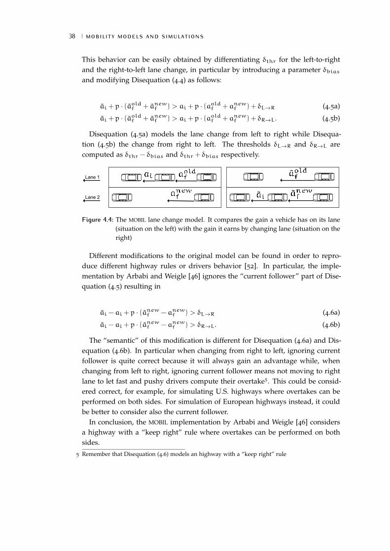
38 MOBILITY MODELS AND SIMULATIONS
This behavior can be easily obtained by differentiating δthr for the left-to-rightand the right-to-left lane change, in particular by introducing a parameter δbiasand modifying Disequation (4.4) as follows:
ai + p · (aoldf + anewf ) > ai + p · (aoldf + anewf ) + δL→R (4.5a)
ai + p · (aoldf + anewf ) > ai + p · (aoldf + anewf ) + δR→L. (4.5b)
Disequation (4.5a) models the lane change from left to right while Disequa-tion (4.5b) the change from right to left. The thresholds δL→R and δR→L arecomputed as δthr − δbias and δthr + δbias respectively.
Lane 1
Lane 2
Figure 4.4: The MOBIL lane change model. It compares the gain a vehicle has on its lane(situation on the left) with the gain it earns by changing lane (situation on theright)
Different modifications to the original model can be found in order to repro-duce different highway rules or drivers behavior [52]. In particular, the imple-mentation by Arbabi and Weigle [46] ignores the “current follower” part of Dise-quation (4.5) resulting in
ai − ai + p · (anewf − anewf ) > δL→R (4.6a)
ai − ai + p · (anewf − anewf ) > δR→L. (4.6b)
The “semantic” of this modification is different for Disequation (4.6a) and Dis-equation (4.6b). In particular when changing from right to left, ignoring currentfollower is quite correct because it will always gain an advantage while, whenchanging from left to right, ignoring current follower means not moving to rightlane to let fast and pushy drivers compute their overtake5. This could be consid-ered correct, for example, for simulating U.S. highways where overtakes can beperformed on both sides. For simulation of European highways instead, it couldbe better to consider also the current follower.
In conclusion, the MOBIL implementation by Arbabi and Weigle [46] considersa highway with a “keep right” rule where overtakes can be performed on bothsides.
5 Remember that Disequation (4.6) models an highway with a “keep right” rule

4.4 CHANGES IN THE MOBILITY SIMULATOR 39
4.4 CHANGES IN THE MOBILITY SIMULATOR
For the purposes of this thesis the original mobility simulator developed byArbabi and Weigle [46] had to be modified and extended. For example, thestandard used in the original simulator was 802.11a, while for VANET simulation802.11p must be employed. The following sections describe the changes.
4.4.1 Crash simulation and management
First of all the simulator had to take into account car crashes. Collisions areallowed by introducing the more realistic Equation (4.3) in the computation ofvehicles acceleration. Then there was the need to manage the collisions, which aredetected by computing the distance between each pair of consecutives vehicles: ifthe distance is negative an accident has occured.
Listing 4.1 shows how the behavior of the vehicles changes after the crash hasbeen detected. First of all the front vehicle is moved ahead of a quantity equalto their distance: in this way the cars are no more “overlapped”. Then the speedis set for both as the average of their speed. Finally there could be two cases, i.e.the front vehicle has or has not a stronger deceleration w.r.t. the following vehicle.If the front vehicle has not a stronger deceleration than the other, then they willcontinue with the same deceleration they had before the crash. In the other caseinstead, the following vehicle will push the leader and will remain “glued” to it:so their acceleration is set as the average acceleration. For simplicity Listing 4.1shows the procedure only for two cars but in the simulator the procedure isiterative and it is able to manage a pile-up.
4.4.2 Accelerometer and imperfect clock
Each vehicle has been equipped with an accelerometer, which basically mea-sures the change of speed every 100 ms. This is more realistic than taking the per-fect acceleration computed with the IDM formula. Moreover with the accelerome-ter it is possible to see in the log traces the peaks of acceleration caused by crashes,as shown in Chapter 5.
Another equipment that has been implemented is an imperfect clock, usedto avoid the occurrence of events at the same exact time, which is unrealisticand causes the simulation to generate synchronization phenomena. The clockdrift has been set as a very small value, i.e. 1 minute in a year. Moreover, NS-3 does not consider processing delays, and again this could lead to unrealistic

40 MOBILITY MODELS AND SIMULATIONS
d i s t a n c e = Distance(vehicle, front)
i f ( d i s t a n c e< 0 ) then
front.SetPosition(front.GetPosition() − d i s t a n c e )
avgSpeed = (vehicle.GetSpeed() + front.GetSpeed()) / 2
front.SetSpeed ( avgSpeed )vehicle.SetSpeed ( avgSpeed )
i f ( front.GetAcceleration() < vehicle.GetAcceleration() ) then
avgAcc = (vehicle.GetAcceleration() + front.GetAcceleration()) / 2
front.SetAcceleration ( avgAcc )vehicle.SetAcceleration ( avgAcc )
end i f
end i f
Listing 4.1: Crash management
synchonizations. So every send and receive event has been delayed by a randomtime between 0 and 10 µs.
4.4.3 CACC
Another fundamental component to implement was a CACC, which has theduty of processing data received from other vehicles to keep safety distance andbrake if the driver does not react in time to a dangerous situation. As describedin the introduction, the CACC considered in this thesis does not implement a carfollowing procedure. The CACC is very simple: to develop a realistic CACC is notthe aim of the thesis.

4.4 CHANGES IN THE MOBILITY SIMULATOR 41
First of all, if the approaching rate is negative (i.e., leading vehicle is travellingfaster than its follower), then the vehicles are automatically increasing their gap,so the CACC remains disabled6.
If instead the approaching rate is positive, the CACC must compute the safetygap to determine if a vehicle is too close to its leader. Safety gap clearly dependson the speed of the vehicle, so it is computed as
ssafe = Tcacc · υi + εcacc
where Tcacc is the time headway for the CACC, υi is the current vehicle speed andεcacc is a small quantity to account for errors. Tcacc has been set to 1 s which,as mentioned in the paper by Treiber et al. [50], is an average time measured onGerman freeways which is considered safe. εcacc has been set to 1 m.
The actual gap between the car and leading vehicle can be greater or lower thanthe safety gap. If it is lower then the follower must brake in order to move awayfrom leader. The applied deceleration can be computed from leader accelerationminus a small quantity. If instead the actual gap is greater than the safety gap theCACC computes a deceleration using the following formula:
acacc =υ2i+1 − υ
2i
2 · (sactual − ssafe)
which computes the acceleration needed to bring the speed of following vehicle(υi) to the speed of its leader (υi+1) in a space equal to the difference between theactual gap (sactual) and the safety gap ssafe).
Notice that if the driver (i.e., the IDM model) decides to brake harder than theCACC, the latter will let the car decelerate as the driver chooses. As a final andimportant feature, the CACC will not perform any operation if data about frontvehicle is outdated more than three seconds.
4.4.4 Air resistance induced deceleration
CACC has been designed to work only with messages regarding front vehicle,but a way to evaluate the benefits of repropagated EEBL messages was needed.The idea here was to use EEBL messages coming from ahead vehicles as warningsdirected to the driver: when received, the simulator reacts as if the driver removes
6 In fact even in this situation if the gap is very small due, for example, to a sudden change of lane,the CACC should brake a little bit in order to increase the gap as soon as possible, but again thedevelopment of a perfect CACC is not the purpose of this thesis

42 MOBILITY MODELS AND SIMULATIONS
his foot from the accelerator pedal, resulting in a deceleration induced by the airresistance. If no EEBL messages are received within two seconds, this mechanismis disabled and the vehicle returns to obey the IDM formula. The drag force canbe computed using
Fdrag =1
2ρυ2CDA. (4.7)
Equation (4.7) is known as the drag equation [53] and computes the force abody with a section A and a drag coefficient CD is subjected if it runs at a speedυ in a fluid of density ρ. Final deceleration has been computed as a function ofspeed
bair =Fdrag(υ)
1500kg
using ρ = 1.20 kg/m3 (air at 20°C), for a vehicle weight of 1500 kg. The CDAproduct is randomly set for each vehicle using values for common productioncars found on an unofficial site [54]. As a result the air drag deceleration canresult in a maximum of 1 m/s2 for a speed of 40 m/s (roughly 150 km/h).
This is a simplification of a complex human behavior which could be enhancedgiving a weight to the warning according, for example, to the distance. Anyhowthis is left as a future work.
4.5 NETWORK PROTOCOLS
The EEBL application clearly requires the definition of some simple networkprotocols to diffuse information among vehicles. The first one is a beaconingprotocol: this is very simple but fundamental to give the CACC “an idea” aboutnearby vehicles, in particular about the front car. Without beacon messages therecould be the possibility that a driver gets so close to its leader that, if the latterstarts braking, even the CACC would not be able to avoid a crash. With beaconsinstead, the CACC can make the car respect the safety distance and easily avoida crash even in the case of a violent braking. Notice that every car which isequipped with the EEBL application is also equipped with the CACC.
The beaconing protocol simply broadcast messages at a frequency of 1 Hz: mes-sages must contain informations about sender vehicle, such as speed, acceleration,position, etc. . . . The same packet definition has been used for beacons and EEBL
messages, following the indications of U.S. DOT [6]: Table 4.1 shows the fields.

4.5 NETWORK PROTOCOLS 43
Moreover, a header has been defined to meet other application requirements, forexample sender identification. Table 4.2 lists the fields:
TYPE determines if the packet is a beacon, an EEBL message or an aggregatedEEBL message;
PACKET ID is used as a unique identificator for the packet for statistical purposes.In a real scenario it could be thought as a sequence number;
ORIGINATOR ID is the id of the vehicle which has created the message, or better,the vehicle that the packet describes;
TTL is the time-to-live of the packet in hops. Initially it is set to 0 for beacons andfor EEBL messages which must not be rebroadcasted, otherwise it is set as 5;
SENDER ID is the id of the vehicle which has actually sent the message. In thecase of a rebroadcasted EEBL message, it is different from the originator id;
COUNT tells, in the case of an aggregated EEBL message, how many packets havebeen inserted;
CERTIFICATE is the digital certificate of the originator, for authentication pur-poses7. In the simulation it is not used, but it must be included in order toproperly analyze network load. The size of 58 bytes is taken from Ibrahimand Weigle [42];
DIGITAL SIGNATURE is the signature of the originator. As for the certificate, it isnot actually used in the simulation and its size is taken from Ibrahim andWeigle [42].
The EEBL protocol is very simple. It works exactly as the beacon protocol, butmessage frequency is 10 Hz as indicated by U.S. DOT [6]. Switching between bea-coning and EEBL protocol happens when the deceleration of the vehicle is strongerthan 1 m/s2 (i.e., an acceleration of -1 m/s2). Moreover, packets coming from be-hind vehicles or from vehicles running in the opposite direction8 are ignored.
Slightly more complicated is instead the EEBLR protocol, in which more appli-cation logic must be used as shown in Listing 4.2. First of all, when a packetis received, the protocol must determine if it the first time it sees the packet: to
7 In the case of rebroadcast a single certificate (with a single signature) is not enough because thereceiver is interested in the “full chain”, from the originator to the last rebroadcaster. However,security in VANETs is a problem in its own and the development of a secure protocol goes beyondthe scope of this thesis
8 The two-directional highway has not been considered but this simple control has anyhow beenimplemented
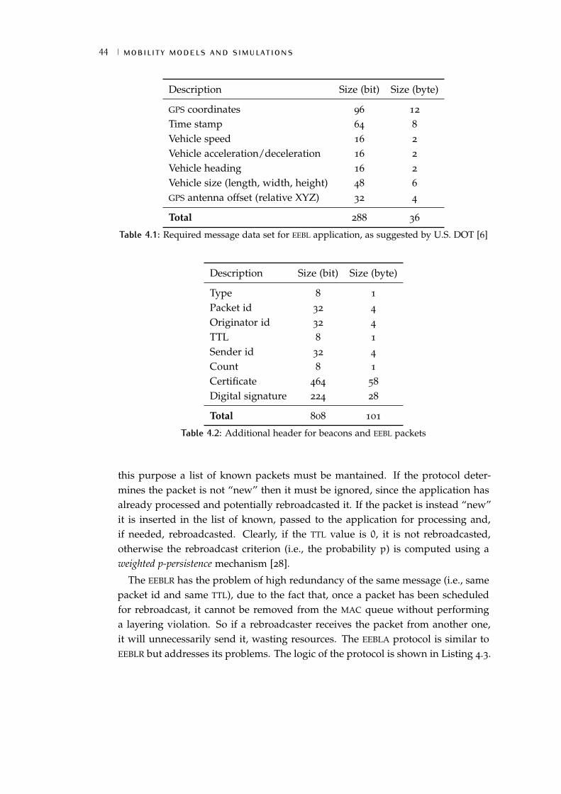
44 MOBILITY MODELS AND SIMULATIONS
Description Size (bit) Size (byte)
GPS coordinates 96 12
Time stamp 64 8
Vehicle speed 16 2
Vehicle acceleration/deceleration 16 2
Vehicle heading 16 2
Vehicle size (length, width, height) 48 6
GPS antenna offset (relative XYZ) 32 4
Total 288 36
Table 4.1: Required message data set for EEBL application, as suggested by U.S. DOT [6]
Description Size (bit) Size (byte)
Type 8 1
Packet id 32 4
Originator id 32 4
TTL 8 1
Sender id 32 4
Count 8 1
Certificate 464 58
Digital signature 224 28
Total 808 101
Table 4.2: Additional header for beacons and EEBL packets
this purpose a list of known packets must be mantained. If the protocol deter-mines the packet is not “new” then it must be ignored, since the application hasalready processed and potentially rebroadcasted it. If the packet is instead “new”it is inserted in the list of known, passed to the application for processing and,if needed, rebroadcasted. Clearly, if the TTL value is 0, it is not rebroadcasted,otherwise the rebroadcast criterion (i.e., the probability p) is computed using aweighted p-persistence mechanism [28].
The EEBLR has the problem of high redundancy of the same message (i.e., samepacket id and same TTL), due to the fact that, once a packet has been scheduledfor rebroadcast, it cannot be removed from the MAC queue without performinga layering violation. So if a rebroadcaster receives the packet from another one,it will unnecessarily send it, wasting resources. The EEBLA protocol is similar toEEBLR but addresses its problems. The logic of the protocol is shown in Listing 4.3.

4.5 NETWORK PROTOCOLS 45
l i s t KnownPackets
on InitProgram():KnownPackets← ∅
on ReceiveEEBLPacket(eebl):i f (KnownPackets.Contains(eebl) ) then
returnelseKnownPackets.Insert(eebl)ProcessPacket(eebl)i f (eebl.ttl 6= 0 )p← ComputeRebroadcastProbability(eebl)i f ( Random() < p )eebl.ttl← eebl.ttl− 1Broadcast(eebl)
end i fend i f
end i f
Listing 4.2: The EEBLR protocol
The idea is to use a queue for packets which is emptied every 100 ms. Withthis mechanism, since the packets are queued at the application layer, uselessrebroadcast can be avoided. Moreover, if more messages are contained in thequeue, a single packet can be sent, reducing overhead.
The pseudocode of EEBLA is similar to the one in Listing 4.2 with some changes.First of all, upon reception of an aggregated EEBL message, every single packet isprocessed by the ReceiveEEBLPacket procedure. If the packet is known, beforebeing ignored, it is removed from the send queue if present, since someone elsehas already rebroadcasted it. If instead the packet is not known and the rebroad-cast criterion is satisfied (the same of EEBLR) it is inserted into the send queue,which is emptied every 100 ms by the SendPackets procedure.

46 MOBILITY MODELS AND SIMULATIONS
l i s t KnownPackets
l i s t SendQueue
on InitProgram():KnownPackets← ∅SendQueue← ∅ScheduleEvent(SendPackets, 100ms)
on ReceiveAggregatedEEBLPacket(aggregatedeebl):foreach (eebl in aggregatedeebl )
ReceiveEEBLPacket(eebl):
on ReceiveEEBLPacket(eebl):i f (KnownPackets.Contains(eebl) ) then
i f (SendQueue.Contains(eebl) )SendQueue.Remove(eebl )
end i freturn
elseKnownPackets.Insert(eebl)ProcessPacket(eebl)i f (eebl.ttl 6= 0 )p← ComputeRebroadcastProbability(eebl)i f ( Random() < p )eebl.ttl← eebl.ttl− 1SendQueue.Insert(eebl)
end i fend i f
end i f
on SendPackets():i f (SendQueue.Size() 6= 0 ) then
i f (SendQueue.Size() = 1 ) thenpacket← SendQueue.Get(0)
e lsepacket← CreateAggregatedPacket(SendQueue)
end i fBroadcast(packet)SendQueue.Empty()
end i fScheduleEvent(SendPackets, 100ms)
Listing 4.3: The EEBLA protocol

5 P E R F O R M E D T E S T S
The tests that have been performed for EEBL protocol and application analysisreproduce the scenario in which the leader of a platoon of vehicles performsa complete stop (e.g., when an accident occures on the highway). Basically theleader (or the leaders, in the multi-lane scenario) performs a brake with a constantdeceleration of 4 m/s2. Different kind of simulations have been done in order toanalyze different aspects of the EEBL application, for example network load andthe reduction of the number of crashes.
Tests can be divided into five big classes, that are the models that have beentested:
PURE IDM which reproduces the scenario with the IDM model as originally de-scribed by Treiber et al. [47]: cars use no VANET technologies. This is impor-tant to show how violent and unrealistic the deceleration of a vehicle underthe IDM model can be;
LIMITED IDM which uses the IDM model with the maximum deceleration, as de-scribed in Section 4.2, Equation (4.3). In this way it is possible to have anidea of the number of crashes that occure. As for pure IDM, VANET technolo-gies are not employed;
EEBL test uses beaconing and EEBL protocol without any kind of rebroadcast. Themaximum deceleration for IDM has been used;
EEBL WITH REBROADCAST test uses beaconing and EEBLR protocol;
EEBL WITH AGGREGATION test uses beaconing and EEBLA protocol.
What have been investigated are first of all the benefits an EEBL system canprovide if all vehicles are equipped with this VANET technology. This test hasbeen performed with a single lane, fifty vehicles and six different average speedsthat are 13.88, 19.44, 25, 30.55, 36.11, 41.66 m/s (50, 70, 90, 110, 130, 150 km/h).Each test has been repeated twenty times with different initial conditions. Whatis analyzed here are the percentages of cars crashed, the average maximum decel-erations, the traces in time of the accelerations and the network load to initiallyidentify the differences between the EEBL protocols.
47

48 PERFORMED TESTS
The first test has then been extended to a multi-lane scenario and it has beeninvestigated by the point of the network, analyzing the differences between EEBLR
and EEBLA. Tests have been performed with 1, 2, 3, 4 and 5 lanes, fifty vehicles perlane at an average speed of 36.11 m/s (130 km/h). Each test has been repeatedtwenty times.
Second a market penetration rate analysis has been performed. The penetrationrate indicates the fraction of vehicles that are equipped with the EEBL application.The aim is to determine if it is possible to gain benefits even if not all vehicles usethis technology because, clearly, it will not be deployed in a single day worldwide.As before, tests are performed on a single lane with fifty cars at six differentaverage speeds. Penetration rates used are 0%, 10% to 40% in steps of 2%, and50%. This time each single test have been repeated thirty times to have a moreprecise indication of the percentage of crashes. Accidents have been investigatedby comparing the results obtained with EEBL, EEBLR and EEBLA and by analyzingthe differences between equipped and unequipped vehicles.
Finally the market penetration rate analysis has been done in the multi-lanescenario, with 2, 3, 4 and 5 lanes at an average speed of 36.11 m/s (130 km/h).Penetration rates have been reduced to 10, 20, 25, 30, 35, 40 and 50% due tothe high computational requirements of the multi-lane simulation. For the samereason, each test has been repeated twenty times instead of thirty.
5.1 SIMULATION PARAMETERS
To perform all the simulations the same set of parameters has been used. Ta-ble 5.1 lists the values for IDM parameters. Cars maximum deceleration (whenused) has been set randomly in the interval [5.9, 8.4] obtained by U.S. DOT [6] indry surface conditions. The desired speed has also been set randomly as the aver-age speed of the simulation ± 15%. Desired deceleration has been set to -4 m/s2,which is quite a big value but the aim is to verify what happens in particularlydangerous situation, and so also T ranges randomly between 0.1 (very aggressivedriver) and 1.1 s (safe driver). Finally, so and δ has been taken from the originalIDM paper [47].
The second set of parameters (shown in Table 5.2) is for MOBIL. The politenessfactor p ranges randomly between 0 (totally impolite) and 0.5 (very polite). Thebsafe parameter has been set so that 7 m/s2 is the maximum deceleration a drivercan cause to incoming vehicles by changing lane. Minimum gap smin has beenset to 2 m, δthr to 0.3 m/s2 and δbias to 0.2 m/s2. So δR→L and δL→R were 0.5and 0.1 m/s2 respectively.

5.1 SIMULATION PARAMETERS 49
Parameter Value Unit
bmax [5.9, 8.4] m/s2
υdes υ · [0.85, 1.15] (±15%) m/sa 1.7 m/s2
b −4 m/s2
T [0.1, 1.1] ss0 2 mδ 4 #
Table 5.1: IDM parameters used in simulations
Parameter Value Unit
p [0, 0.5] #bsafe 7 m/s2
smin 2 mδthr 0.3 m/s2
δbias 0.2 m/s2
Table 5.2: MOBIL parameters used in simulations
Final parameters needed are the ones related to the wireless communications,which are listed in Table 5.3. Clearly, the 802.11p standard has been selectedand two different ACs have been used for beacons and EEBL messages, i.e. AC_BK
and AC_VO respectively. Selected datarate is 6 Mbps with a bandwidth of 10
MHz (as 802.11p mandates) and a transmission power of 20 dBm. To model thepropagation loss, the “three log distance” of NS-3 with default parameters hasbeen used1. This model computes the loss of power as a function of the distance:in particular the loss is logarithmic w.r.t. the distance, computed as
L = L0 + 10 ·n0 log10
(d
d0
)(dB)
where L0 (dB) is the path loss at reference distance d0 (m), d (m) is the distanceand n0 (unitless) is the path loss exponent.
1 http://www.nsnam.org/doxygen-release/classns3_1_1_three_log_distance_propagation_
loss_model.html

50 PERFORMED TESTS
The three log model uses three different distance fields resulting in the follow-ing final formulation:
L =
0 d < d0
L0 + 10·n0 log10(dd0
)d0 6 d < d1
L0 + 10·n0 log10(d1d0
)+ 10·n1 log10
(dd1
)d1 6 d < d2
L0 + 10·n0 log10(d1d0
)+ 10·n1 log10
(d2d1
)+ 10·n2 log10
(dd2
)d2 6 d
where d0, d1 and d2 (m) are the three distance fields, d (m) is the distance, L0(dB) is the path loss at reference distance and n0, n1 and n2 (unitless) are thepath loss exponents for the fields.
Parameter Value Unit
IEEE standard 802.11p CCH
AC (beacons) AC_BK
AC (EEBL) AC_VO
Data rate 6 MbpsBandwidth 10 MHzTx power 20 dBmPropagation loss Three log distance
Table 5.3: Network parameters
5.2 SINGLE LANE TESTS
Figure 5.1a shows a trace in time of the acceleration of the first thirteen vehicles,from the moment in which the first vehicle starts braking. The deceleration of thefirst vehicle is fixed at 4 m/s2, while the followers use the acceleration providedby the model. In particular, vehicles number 12 and 13 reach a deceleration largerthan 1 G, which is not possible with common production cars [49, 48]. Figure 5.1binstead is focused on first five vehicles for a better understanding: it is possibleto see that the model can result in different “braking forces” depending on theaggressiveness of the driver. Moreover, after having stopped, drivers re-accelerateto come closer to their leader, which is a common situation.
The modification done to IDM (Section 4.2, Equation (4.3)) results in crashes. Itis possible to see in Figure 5.2 the peaks of acceleration and deceleration caused byrear end collisions. Figure 5.2a shows a collision between two vehicles, in particu-

5.2 SINGLE LANE TESTS 51
(a) First thirteen vehicles (b) First five vehicles
Figure 5.1: Trace of the accelerations in time for pure idm test, 41.66 m/s
lar V3 which collides with V2 (notice the deceleration of V3 and the accelerationof V2) while Figure 5.2b shows a pile-up of three cars (V3, V2 and V1).
(a) 36.11 m/s (b) 41.66 m/s
Figure 5.2: Trace of the accelerations in time of the first five vehicles for the limited idm
test
So the first question to be answered is: can an EEBL system improve the safety ofa highway? The answer is straightforward, but it must be justified and quantified.In particular Figure 5.3a shows the percentage of vehicles involved in a crash, witha 95% confidence interval, as a function of the speed. Just to clarify, if vehicles A,B, C and D are involved in a pile-up, then four vehicles are counted. Obviously,pure idm results in a crash free scenario, since it is a car following model, while

52 PERFORMED TESTS
(a) Crash percentages (b) Average maximum deceleration
Figure 5.3: Quantification of the benefits of an EEBL system, for a 100% market penetra-tion rate
limited idm results in an increase of crashes with a non-linear growth. This resultobtained by the simulation reflects what happens in reality [55]2.
For a 100% market penetration rate, the EEBL system integrated with the CACC
would completely avoid crashes, whatever the protocol. Clearly we are assumingthat drivers never perform a sharp steering to avoid a collision: in such case nosystem can avoid a disaster, unless the on-board computer completely controls thecar, which is unlikely. The result could seem straightforward: if all vehicles areequipped then the situation is always under control. However this assumptioncannot be given a priori: if, for example, the EEBLR protocol is so “aggressive”that the number of collisions (in the network) causes a lack of information to theCACC, possible dangerous situations could happen.
Figure 5.3b shows the average maximum decelerations for the various tests. Toobtain the results, the acceleration of all vehicles have been monitored duringsimulations: at the end the maximum values of deceleration have been averagedand plotted with a 95% confidence interval. The experiments with pure idm
and limited idm show an average maximum deceleration which is always higherthan 4 m/s2 (the deceleration of the first vehicle). limited idm is “softer”, butonly because vehicles cannot brake stronger than a certain limit. For the EEBL
enabled experiments instead the deceleration is very smooth. This is important
2 Indeed in the cited report the authors found an exponenential relationship between speed andcrash risk. In this thesis it is not possible to analyze such relationship because only six speeds havebeen considered. Moreover, it is not in the aims of this work to reproduce a real crash model. Theimportant thing here is not having a linear relationship, because real world is not like that (as faras Kloeden et al. have discovered)

5.2 SINGLE LANE TESTS 53
for safety: if an automated system performs a violent braking maneuver on a wetroad, consequences can be devastating.
From the point of view of the automotive field, the deceleration could be con-sidered too weak, with possible negative influences on traffic flow. However thisresult is due to the “naïveness” of the implemented CACC: desired decelerationcould be parameterized (as for IDM) and increased, without harming the overallsafety. A deceleration of 2-3 m/s2 can be considered safe even on wet floors,where decelerations of 6 m/s2 can be easily reached [49]. On icy roads the prob-lem would come up again, but in that case a specialized study should be done.
At this stage of the results it could seem that EEBLR and EEBLA give no bene-fits and are only a waste of resources. In Figure 5.3 EEBL, EEBLR and EEBLA areindistinguishable. But it is important to remember that till now a full marketpenetration rate is considered, and we have not yet analyzed the network load.
The reason why the average maximum deceleration is so low, is shown in Fig-ure 5.4: in the pure idm test, vehicles behind the leader brake harder than it, whilewith the CACC the deceleration becomes more and more smooth. This is for surea benefit due to the safety distance mantained by the CACC. This result could bethe basis for the study of a CACC which minimizes the inter-vehicle distance, toimprove traffic flow. A lower safety distance, would result in a stronger deceler-ation, which could be calibrated in order to maximize traffic flow while keepingthe risk of accidents under control: again this is not the aim of the thesis.
In Figure 5.4 moreover, it is possible to notice again the similarity betweenEEBL, EEBLR and EEBLA from the point of view of the automotive application. Itis important to give some more details about those pictures (e.g., Figure 5.4b):first of all it is possible to notice the deceleration caused by the air drag forcefor vehicle 5. When it receives the EEBL message from first vehicles, the driverremoves its foot from the accelerator pedal and the car begins to decelerate dueto air resistance. Then when vehicle 4 starts braking harder and sending EEBL
messages, the CACC of vehicle 5 starts reacting.When vehicle 2 reaches 1 m/s2 of deceleration, it switches from EEBL protocol
to normal beaconing: however the system still performs well3. This is due to theimplementation of the CACC: in the case of missing packets it predicts positionand speed of front vehicle using previously collected data and applying simplephysics formulas (e.g., x(t) = v(t) ·∆t+ x0). Finally a little peak of decelerationoccurs due to the IDM model: basically “the driver” wants to apply a brake forcestronger than the CACC, so the latter leaves the control to IDM.
Given the results of the application-oriented analysis, it is possible to start withnetwork load characterization. Figure 5.6 shows a three-dimensional representa-
3 In fact it is possible to see small imperfections, but they are very difficult to notice
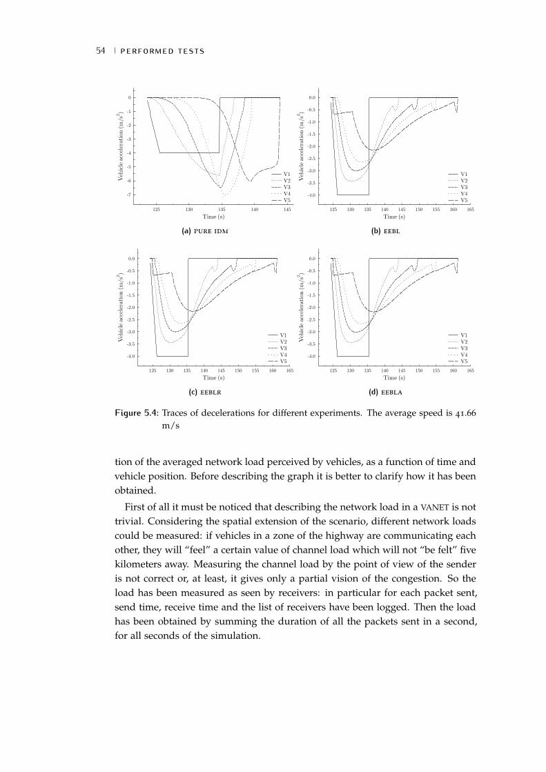
54 PERFORMED TESTS
(a) pure idm (b) eebl
(c) eeblr (d) eebla
Figure 5.4: Traces of decelerations for different experiments. The average speed is 41.66
m/s
tion of the averaged network load perceived by vehicles, as a function of time andvehicle position. Before describing the graph it is better to clarify how it has beenobtained.
First of all it must be noticed that describing the network load in a VANET is nottrivial. Considering the spatial extension of the scenario, different network loadscould be measured: if vehicles in a zone of the highway are communicating eachother, they will “feel” a certain value of channel load which will not “be felt” fivekilometers away. Measuring the channel load by the point of view of the senderis not correct or, at least, it gives only a partial vision of the congestion. So theload has been measured as seen by receivers: in particular for each packet sent,send time, receive time and the list of receivers have been logged. Then the loadhas been obtained by summing the duration of all the packets sent in a second,for all seconds of the simulation.

5.2 SINGLE LANE TESTS 55
To be more formal, if Txi and Rxi are the transmission and reception time (inmicroseconds)4 respectively and v the vehicle that has received the packet thenthe load can be computed as shown in Listing 5.1. In particular the first thingto do is determine the “slot” of seconds in which packet must be counted: ifTxi = 10123456µs then the packet must be counted in the range between 10 and11 seconds of simulation. If secondsTx is different from secondsRx then thetransmission began in a second and ended in the successive. For example, ifTxi = 10999900 and Rxi = 11000200 then 100 µs must be counted in the tenthseconds slot, while the other 200 in the eleventh seconds slot.
secondsTx = bTxi/106csecondsRx = bRxi/106c
i f (secondsTx = secondsRx ) thenload[v][secondsTx]+ = (Rxi − Txi)/10
6
e lsefirstAmount = (secondsTx+ 1)× 106 − Txiload[v][secondsTx]+ = firstAmount/106
load[v][secondsRx]+ = (Rxi − Txi − firstAmount)/106
end i f
Listing 5.1: Channel load computation
This procedure is not accurate enough because it does not account for situa-tions like the one in Figure 5.5. In such case the algorithm in Listing 5.1 wouldcount Rx1 − Tx1 + Rx2 − Tx2 which is not correct. So an algorithm to merge suchsituations (so that the load is computed as Rx2 − Tx1) have been developed andused for channel load measurement.
Frame 1
Backoff
Backoff
Frame 2
Backoff Frame 3
V1
V2
V3Defer
Tx1 Rx1
Tx2 Rx2
Figure 5.5: Contention for the channel
At the end of the computation the matrix load contains the perceived loadfor each vehicle for each second of simulation. Then the vehicles are sorted as
4 N.B.: Txi indicates the time at which the application passes the packet to the MAC layer, while Rxithe time at which the packet is delivered to the application by the MAC layer

56 PERFORMED TESTS
a function of their distance from the first vehicle of the simulation, obtaining amatrix pos such that
pos[i][t] = id of the i-th vehicle in distance from first vehicle at time t.
Then elements are re-arranged so that a new load matrix sortedLoad is ob-tained:
sortedLoad[i][t] = load[pos[i][t]][t]. (5.1)
The matrix obtained by Equation (5.1) is identical to the matrix of Listing 5.1 inthe case of a single lane, while this is not true in the multi-lane scenario, whereovertakes occur. This sorted matrix is important because otherwise the resultinggraph would mix the loads of vehicles which are in complete different locations ofthe scenario. For example, imagine that a vehicle at the end of the platoon5 is sofast that it overtakes all vehicles up to the leaders: with the matrix of Listing 5.1,its load value would be plotted in the rightmost part of the graph, which is notcorrect, since the vehicle is together with the firsts in the platoon.
If a test is repeated twenty times, twenty matrices are obtained. These matricesare averaged and the result is used to finally plot the colormap.
Even with such solution the load would not tell the true story, because collidedpackets do not have receivers, so their load cannot be computed. In the pres-ence of collisions, the load would be underestimated. So an analysis of packetcollisions has been performed (described later).
As a final remark, notice that the computation of the load takes into accountalso AIFS and backoff procedure6, which is correct. The channel is consideredbusy in those periods because it cannot be accessed.
Now it is possible to come back to Figure 5.6: on the abscissa there are vehiclesordered by position, while on the ordinate the time. The first thing to notice isthe black triangle on the bottom, which is due to the fact that vehicles are injectedwhile the simulation runs, so at the beginning not all vehicles are present. Thenthe purple stripe indicates a low load zone due to the beaconing: one packetper second for fifty vehicles does not create any problem. Moreover the distancemakes the load even lower, because packets of first vehicles are not received by ve-hicles at the end of the platoon, and viceversa. To give a theoretical quantificationof the load it is possible to adapt Equation (2.2) for beacons. For the AC_BK (the
5 If a vehicle is one of the last that has “joined” the simulation it has a high id, since id are given tothe vehicles in the order they are injected in the highway
6 Because send time considers the moment in which the packet is passed to the MAC layer

5.2 SINGLE LANE TESTS 57
AC used for beacons) the AIFS value is 9 slots (so 117 µs) while the backoff on av-erage should be 97.5 µs (because CWmin is 15 slots). Then the load for beaconingprotocol is:
Loadbeacon(n) =486µs ·n1s
· 100(%). (5.2)
However Equation (5.2) is not very correct in this particular case. Due to thelow load, all nodes will very probably find the channel free when trying to senda packet. Following the CSMA rules, they will access the channel immediately,without waiting for AIFS and without performing the backoff procedure and so amore correct formulation is
Loadbeacon(n) =272µs ·n1s
· 100(%). (5.3)
Later the correctness of Equation (5.3) will be empirically proved.At roughly 150 seconds the first vehicle starts braking and sending EEBL mes-
sages. Consequently, its followers do the same, so the network load rapidly in-creases up to 2%, as shown by the light blue stain. Here it must be noticed thatthe load increases only for the first fifteen vehicles, which is a consequence ofhow the CACC works: by looking back at Figure 5.4b, the maximum decelerationdecreases more and more while going far away from first vehicle. As a result,some vehicles never decelerate stronger than 1 m/s2 so they never send an EEBL
message. This has clearly positive effects on the network: some vehicles (between10 and 15) perceive an increase of network load for a smaller amount of time.Now consider again the statement written to comment Figure 5.3: by redesigningthe CACC in order to have a stronger deceleration and improve traffic flow, thenetwork load would increase. This is an important result which emphasizes theneed to take into accont the dependency between the application and the networkprotocol.
After the severe braking phase, the platoon starts to “compact”. This producesan increase of the network load because more vehicles move in the transmissionrange of the others and more and more beacons are received as time elapses.By looking at first vehicles (1 to 10) it is possible to se a shade from purple toblue. Central vehicles instead feel the increase before the others, because they canreceive packets from the front and the end of the platoon. Final vehicles insteadare clearly the last to perceive the increment. A further analysis of this dynamicis given in Section 5.3.
Now it is possible to show empirically that Equation (5.3) is correct. In the caseof fifty vehicles, the equation would result in a load of 1.36% which agrees withthe blue zone at the top of the graph.

58 PERFORMED TESTS
Figure 5.6: Network load for eebl experiment, one lane 36.11 m/s
Figure 5.7 shows the loads produced by the EEBLR and EEBLA protocols. Thefigures are similar to the situation of Figure 5.6, because the dynamics of thevehicles are the same. What changes is clearly the network load: in particular,EEBLR reaches an average maximum of 7%, while EEBLA roughly 4%. So the loadof EEBLR is more than tripled w.r.t. normal EEBL, while EEBLA is doubled. Noticethat doubling the load of the network with a repropagation protocol is somehownatural. Imagine that vehicle A in Figure 5.8 broadcasts a packet and vehicle Brepropagates it: vehicles in their transmission range will clearly receive the packettwice, there is no way to avoid it.
It is possible to see that the color stain caused by the braking is spread in timeand space, because the information disseminates farther thanks to repropagation.
(a) eeblr (b) eebla
Figure 5.7: Network load for eeblr and eebla experiments, one lane 36.11 m/s

5.3 MULTI LANE TESTS 59
Lane 1
Lane 2
Lane 3
A CB D
E F
H
G
I
Tx Range of A
Tx Range of B
A MSG A MSG
Figure 5.8: Natural doubling of network load due to message repropagation
To conclude this section one more graph is presented. Given the load matrixof Equation (5.1), the set of maximum load values have been extracted. Moreformally:
maxValues[exp][i] = maxt∈T
sortedLoadexp[i][t] exp ∈ [1, . . . ,Nexp].
These values have been used to plot a Cumulative Distribution Function (CDF),so to determine the number of vehicles having “noticed” a maximum load lowerthan a certain value, for all experiments together. The results are shown in Fig-ure 5.9: the ordinate axis has been normalized.
The eebl experiment shows a complete different trend w.r.t. the other two. Thisis probably given by the fact that the EEBL protocol during the braking phase hasmore or less the same load as the beaconing at the end of the simulation, so almostall vehicles have “felt” the same maximum value. For EEBLR and EEBLA instead,the load during the braking phase is much higher, so the CDF changes. Comparingthe eeblr experiment with eebla it is possible to see that EEBLR protocol has anoverall maximum slightly more than 12%, while EEBLA reaches 8%. Those valuestell that loads of Figure 5.6 and Figure 5.7 are not the real maximum, but this isclearly due to averaging. In Figure 5.9a indeed the maximum obtained is 2.6%and not 2%.
5.3 MULTI LANE TESTS
In this section the multi-lane scenario will be analyzed by the point of view ofthe network, since no crashes occured in any tests with EEBL. To continue with theanalysis given in the last part of previous section, Figure 5.10 shows the networkload for the five lane test, with 250 vehicles. The “graphical aspect” is the same asin Figure 5.6 and Figure 5.7, but clearly the scale changes. In particular the eebl
test reaches 10% during the braking phase, so there is a linear increase w.r.t. thenumber of vehicles, which is quite obvious.

60 PERFORMED TESTS
(a) eebl (b) eeblr
(c) eebla
Figure 5.9: CDFs of maximum loads of all single-lane experiments, for average speed 36.11
m/s
The maximum load of the eeblr test is again more than tripled, reaching up to36%. This may seem a safe limit: still two thirds of the channel time are free andthe simulation has a large number of vehicles. However some observations are inorder:
1. as said before, collided packets are not counted in the network load. Lateron the collisions will be analyzed and it will be shown that the situation ismuch worse;
2. as in one lane test, the design of the CACC makes the majority of the vehiclesbrake with a deceleration lower than 1 m/s2, so for the majority of thevehicles no EEBL message is ever sent;
3. lanes in the opposite direction are not considered. Having other five lanescan further worsen the situation. Probably in most cases the opposite lanes

5.3 MULTI LANE TESTS 61
would not broadcast other EEBL messages but this cannot be given for sure,for example when accidents regards both directions7.
The eebla experiment instead shows a maximum of roughly 26%. It is 10% lessthan eeblr and 2.6 times more than in the eebl experiment.
Finally, Figure 5.10d shows the load for the eeblr test with five lanes but thistime the colormap is drawn as a function of the distance from first vehicle. Theportion of highway behind the leader has been divided into blocks of 50 meterseach. Then the load of each block has been computed as the average load of thevehicles in that block. This representation gives a better idea of the dynamics ofthe platoon and their consequences on the network load. The black triangle at thebottom of the image remains as before. The platoon reaches roughly 4.5 km ofextension and then leaders begin to brake. It is possible to see how the size of theplatoon decreases down to roughly 500 meters: as the group of vehicles decreasesin size, the load of the network increases, as shown by the light blue zone at thetop of the figure.
To further analyze the consequences of the protocols on network load two moregraphs have been plotted. The first one measures the percentage of packets thathave not been received by any vehicle during the braking phase, with a confi-dence interval of 95%. This is not the same as measuring the number of collisions:indeed if a vehicle is alone in the highway its messages will not be received byanybody, but this does not mean that they had a collision. However, given thedensity of vehicles in the scenario, the measure should give a very good approx-imation. The reason why this measure has been taken into account, instead ofcounting the number of collisions, is that NS-3 does not have any way to measurethem. Indeed, since the simulator reproduces quite faithfully the reality, situa-tions as in Figure 5.11 are ambiguous. If vehicles A and D send a message at thesame time, vehicle C will most probably not be able to receive them (so a collisionis counted), while vehicle B will probably get the message, since the packet of ve-hicle D will only be heard as background noise due to signal attenuation. Thesecond graph instead counts the number of packets that vehicles try to send foreach second of the simulation, including received and unreceived.
Figure 5.12 shows the first graph. As said in the previous paragraph, the per-centage of unreceived packets has been analyzed during the braking phase. Thisperiod starts when leaders begin to brake and ends when the deceleration of all
7 Remember the accident on the Italian highway A4 in august 2008 when a truck suddenly steeredand invaded the opposite lanes (article (in Italian) http://archiviostorico.corriere.it/2008/
agosto/09/Tir_salta_guardrai_Strage_dell_co_9_080809024.shtml, video http://www.youtube.
com/watch?v=kjajyJEzKGU, last visited 16/02/2011)

62 PERFORMED TESTS
(a) eebl (b) eeblr
(c) eebla (d) eeblr as a function of the distance from firstvehicle
Figure 5.10: Average loads for test with five lanes, average speed 36.11 m/s
vehicles is less than 1 m/s2 and their speed is lower than 8.33 m/s (30 km/h)8.The analysis has been limited in this period because first of all it is the “criticalmoment” for the network and secondly, as it is possible to see from Figure 5.10,the portion of the simulation where the load is very high is only a small fraction,so averaging the values of the whole simulation would lead to an underestimationof the real problem.
By looking at Figure 5.12 it is possible to see the huge amount of unreceivedpackets for the EEBLR protocol. For the one lane scenario, the percentage is 20%,while for five lane the percentage reaches 60%. Notice that this does not meanthat the maximum load of Figure 5.10b must be increased of those percentages.Indeed if, for example, four packets collide, the collision period will last from thebeginning of the first till the end of the last and the frames are overlapped for
8 This is a heuristic choice to try to grab the most critical part of the dynamic in absence of a formaldefinition

5.3 MULTI LANE TESTS 63
Lane 1
Lane 2
Lane 3
A CB D
E F
H
G
I
Tx Range of A
Tx Range of D
Packet of A correctly received
Packets of A and D collide
D MSGA MSG
Figure 5.11: Collision detection problem
the majority of the time, so the load increases of a quantity which is roughly theduration of the biggest frame.
The “enqueue and defer transmission” mechanism of EEBLA instead performsvery well. The percentage of unreceived packet is not zero, neither for EEBLA norfor EEBL, but it is under 1%. This is because the retransmission of a particularpacket is delayed of an amount of time between 0 and 100 ms. This delay permitsthe nodes to detect prior retransmissions and remove relative packet from thesend queue. With EEBLR instead, once a packet has been scheduled for retrans-mission it is sent to the MAC queue, and then it cannot be removed. Notice that adelay of (maximum) 100 ms is good for the application requirements.
This result indicates that the load plotted in Figure 5.10b is underestimated,while the loads of Figure 5.10a and Figure 5.10c are correct.
Figure 5.12: Percentage of packets that have been sent but not received by any node.Average speed 36.11 m/s, 100% market penetration rate
Figure 5.13 shows the second set of graphs. Their “aspect” is similar: theyhave an initial linear increase due to the injection of vehicles in the simulation.Then during the braking phase the number of offered packets suddenly increases

64 PERFORMED TESTS
and finally decreases down to a constant value which is equal to the number ofvehicles, since all nodes are sending one beacon per second.
Now by looking at maximum peaks it is possible to see that they reach, for theeebl experiment, roughly 100, 200, 300, 400 and 500. For the eebla experiment,those peaks reach roughly 200, 450, 700, 900 and 1150 so, as already said before,there is an increase of a factor of slightly more than two. The eeblr experimentinstead shows the aggressiveness of the EEBLR protocol. The peaks here reacharound 500, 1500, 3000, 4000, and 6000, which is definitely too much. Noticethat the EEBLR protocol already implements a broadcast suppression mechanism(i.e., p-persistent rebroadcast [28].), so imagine how devastating could be a pureflooding protocol.
(a) eebl (b) eeblr
(c) eebla
Figure 5.13: Average number of offered packets during the simulation for the differentprotocols. Average speed 36.11 m/s
To further understand the congestion problem, the same CDFs as in Section 5.2have been plotted (Figure 5.14). The trends are basically the same as before: what

5.3 MULTI LANE TESTS 65
changes are clearly the maximum values reached. EEBL goes up to 11.5%, EEBLA
up to 40% while EEBLR up to 50%. Notice that these are absolute maximums and,by considering the 90% of the vehicles, they decrease down to 9% (EEBL), 29%(EEBLA) and 39% (EEBLR). These values show again that EEBLR is aggressive andthat also EEBLA could be improved, which should be somehow easy, given itssimple logic.
(a) eebl (b) eeblr
(c) eebla
Figure 5.14: CDFs of maximum loads of all five-lane experiments, for average speed 36.11
m/s
Till now, the EEBLA protocol has shown to be a good compromise betweennetwork load and information spread, without using any complex mechanismfound in the literature. From the point of view of the application, the CACC worksthe same as with EEBL protocol, so what is the profit in message repropagation?

66 PERFORMED TESTS
5.4 SINGLE LANE MARKET PENETRATION RATE TESTS
The question left open in the previous section finds its answer here. As de-scribed at the beginning of the chapter, the market penetration rate test givesan idea of the benefits of VANET safety applications when not all vehicles areequipped.
Figure 5.15 shows the plot of the percentage of cars crashed (with 95% confi-dence interval) as a function of the market penetration rate, for eebl, eeblr andeebla tests at 36.11 and 41.66 m/s. The graph shows the clear advantages ofmessage repropagation. Both the eeblr and eebla tests have a lower percentageof accidents, due to the fact that drivers are informed of the dangerous situationwith higher probability and in advance, and the simple action of removing thefoot from the accelerator pedal and let the car gently decrease speed reduces therisk of impact. The higher gain is noticeable in the central part of the graph, be-tween 15 and 40%. For market penetratrion rates lower than 15% the differenceis smaller because the low fraction of equipped vehicles limits message repropa-gation. With a 50% rate it is possble to see that the eebl test starts to convergeto the results of the others. The difference between the protocols at 41.66 m/s iseven more evident.
Notice that this result is most probably underestimated because the action ofremoving the foot from the pedal is an oversimplification of the real human be-havior. If a driver receives an EEBL message sent a few vehicles in front it wouldmost probably brake a little bit, thus increasing inter vehicle distance earlier.
(a) 36.11 m/s (b) 41.66 m/s
Figure 5.15: Percentage of cars involved in accidents for single-lane market penetrationrate tests

5.4 SINGLE LANE MARKET PENETRATION RATE TESTS 67
(a) eebl, 36.11 m/s (b) eebl, 41.66 m/s
(c) eebla, 36.11 m/s (d) eebla, 41.66 m/s
Figure 5.16: Percentage of cars crashed divided for equipped and unequipped for thesingle-lane test
A question that could be arisen is whether the EEBL combined with the CACC
gives benefits only to the equipped vehicles. To address this problem the percent-age of cars crashed has been divided for equipped and unequipped and plottedfor all the experiments, with a 95% confidence interval.
The results for the eebl experiment are shown in Figure 5.16a and Figure 5.16b:clearly on the abscissa the 0% market penetration rate has been removed. Thegraph depicts the same trend of Figure 5.15 and shows that the percentage ofcrashed vehicles with the EEBL system is lower than for unequipped, which isquite obvious. The important thing here is that the probability of crash for un-equipped vehicles decresases in the same way as for equipped. The reason is sim-ple: if an EEBL enabled car receives a message and starts decelerating smoothly, itsfollower will also do the same. When vehicles then arrive into the “braking zone”

68 PERFORMED TESTS
their speed will be lower, thus they will not need to perform a violent decelerationand they will most probably avoid a read-end collision.
For the eebla experiment (Figure 5.16c and Figure 5.16d) the result is similar (inthe sense that both equipped and unequipped gain advantages), but the overallpercentage is clearly lower than for the eebl experiment. Moreover in Figure 5.16cthe percentage for equipped vehicles reaches low values much more earlier: witha market penetration rate of 24% the probability is lower than 2.5%, while inFigure 5.16a that probability is reached when the 38-40% of the cars are equipped.The results for the eeblr tests have been omitted, since they are almost identicalto eebla ones.
5.5 MULTI LANE MARKET PENETRATION RATE TESTS
To conclude the experiments, this section shows the market penetration rateresults for the multi-lane scenario. The comparison between the three tests fortwo, three, four and five lanes is shown in Figure 5.17. As for the single lanetest, there is a visible difference between the basic protocol and the ones withrepropagation. This distinction tends to become smaller as the number of lanesincrease and, for the five lane test, the results for the rates 35, 40 and 50% arealmost identical. The reason is explained in Figure 5.18
9: in the single-lane case,if a vehicle is not able to reach directly one of its equipped followers (A and Bin Figure 5.18a) then nobody behind will know about the dangerous situationin advance. With more lanes instead, the message of a braking vehicle could bereceived by a driver on another lane (like B in Figure 5.18b) which will smoothlydecelerate, reducing its risk of collision. After a while, it will have anyhow theneed to brake so it will start sending messages informing other vehicles (such asC). C will then do the same as B, providing information about the situation to thedriver of vehicle D. So now, vehicle D is aware of the danger even if it is too farfrom vehicle A to receive any of its messages.
As for the one lane tests, both equipped and unequipped vehicles can gainadvantages by the presence of an EEBL system as depicted by Figure 5.19. Forunequipped vehicles, the trends of Figure 5.19a and Figure 5.19b are roughly thesame, with EEBLA which has a slightly lower probability of crash. Equipped vehi-cles instead show a completely different trend, emphasizing the results discussedin the previous section: the difference here is even more evident. However this
9 N.B.: the arrows in the picture must not be intended as repropagation, but just represent thefact that a higher density of equipped vehicles increases the probability that “gentle” behaviorspropagate in the platoon

5.5 MULTI LANE MARKET PENETRATION RATE TESTS 69
(a) 2 lanes (b) 3 lanes
(c) 4 lanes (d) 5 lanes
Figure 5.17: Percentage of cars involved in accidents for multi-lane market penetrationrate tests, average speed 36.11 m/s
is not due to a lower number of crashes for the equipped vehicles, indeed theprobability of crash is almost the same in Figure 5.16c and in Figure 5.19b. Whatchanges is the probability of crash for unequipped vehicles, which is higher forthe multi-lane scenario. As depicted by Figure 5.15a and Figure 5.17, the percent-age of crashes (for a 0% market penetration rate, so it is not due the the presenceof the CACC) increases with the number of lanes. This could be reasonable inreality where, after a crash, a vehicle could unintentionally move to the adjacentlane causing another accident. In the simulator however this is somehow strangebecause such realism is not present. This is a consequence of the lane change: inthe single-lane scenario a slow vehicle cannot be overtaken, so faster drivers mustkeep a lower speed. Consequently, the average speed of the platoon is reduced,decreasing the risk of accidents. Anyhow this result does not “nullify” any of theadvantages of the system described in the whole chapter.

70 PERFORMED TESTS
Lane 1 A B
(a) 1 lane
Lane 1
Lane 2
A
Lane 3
B
C
D
E
F
(b) 3 lanes
Figure 5.18: Higher probability of “natural” propagation for a multi-lane highway. Vehi-cles with letters are the equipped ones
(a) eebl (b) eebla
Figure 5.19: Percentage of cars crashed divided for equipped and unequipped for thefive lanes test, average speed 36.11 m/s

6 F U T U R E W O R K
This thesis gives the basis for a deeper analysis in the field of VANETs having an-alyzed for the first time with a joint mobility-network simulator real applicationslike EEBL. The dependency between the application and the network, however,need further investigation. In U.S. DOT [6] tens of safety and non-safety appli-cations are listed: they clearly have to coexist but, from the point of view of thenetwork, they have completely different requirements, in terms of informationspreading and update rate. Both of these requirements should be checked: in-deed this thesis has shown that a greater “spread range” can improve safety andthat with a frequency update lower than mandated systems can perform well1. Asan example, an application dependent protocol for EEBL could use a high updaterate when deceleration increases and a lower update rate when it decreases. Thishas shown to perform good for a CACC but EEBL is thought also for humans wherethe reaction time plays a fundamental role, and so it should be tested. Anothermodification could be to increase the deceleration threshold used to determinewhen EEBL messages should be sent, again analyzing the consequences on theoverall dynamics.
Regarding human behavior modeling, a more sophisticated “emulation”should be implemented because, as already said before, the action of removingthe foot from the accelerator pedal upon reception of an EEBL warning is an over-simplification. Without taking into account complex AI algorithms, a severityvalue could be assigned to an EEBL message as a function of the distance from theoriginal sender (i.e., decrease severity as distance increases) and as a function ofthe lane (i.e., if the originator is on the same lane the severity is maximal, other-wise it is set depending on the lane the receiver is located). Given the severity, the“driver” could perform different operations, from braking smoothly to simply ig-nore the message. Once a better human reaction is developed, an extension to themarket penetration rate test can be done by considering completely unequippedvehicles, vehicles equipped only with a 802.11p network card only (so to simulatecars with acoustic warning) and vehicles equipped with a CACC.
By the point of view of the automotive field it could be interesting to improvethe behavior of the CACC in order to provide a stronger deceleration reducingthe time the platoon needs to compact, while finding a way to keep the network
1 Remember in Section 5.2 where the prediction mechanism of the CACC is described
71

72 FUTURE WORK
traffic under control. Another improvement could be to take into account a realCACC, so to enable an automatic car following mechanism and analyzing againnetwork requirements and the benefits on traffic flow. For a better analysis oftraffic flow properties in general, scenarios different from the simple emergencybrake should be done, for example by emulating a sort of stop and start andobserve if with such systems the “accordion effect” reduces.
The EEBLA algorithm has shown to be a good compromise between applicationand network requirements, without the need of complex methodologies, opposedto the approaches found in the literature. However, given the simplicity of EEBLA,most probably its results on network load could be further improved by some sim-ple modifications, for example using other broadcast suppression mechanisms asthe basis of the algorithm, such as slotted p-persistence [28] and/or data compres-sion. Moreover, the differences on load given by different transmission rangescould be analyzed, without the need of taking into account complex mathemat-ical model as in Torrent-Moreno et al. [43]. To further reduce the network loadlower values of TTL can be tested, but always keeping under control application-level benefits. Reducing the value of TTL reduces the spread range of information,thus decreases the “global knowledge” of the drivers. Finally, a more accuratesimulation of the physical layer must be taken into account. Since this thesis wasfocused on congestion issues a simple propagation loss model had been used; infuture more realistic models can be used, for example considering also fading.
The simulations have been performed using a bunch of parameters derivedfrom the literature. For example, the values for maximum decelerations havebeen obtained from Schultz and Babinchak [49], which is quite an old document.A more recent report is Michigan State Police [48] but it takes into account carsfor the police and it is not known whether those vehicles are more performantthan normal production cars. Recent documents describing this parameter mustbe found in order to use values of vehicles of nowadays. This could give a moreprecise indication of the number of car crashes. Another parameter that could bemodified is the desired deceleration (b in IDM): for this thesis it has been fixedto a value of -4 m/s2, in order to have quite critical situations. For high-fidelitymodeling, values of deceleration used by real drivers could be searched: if nostatistics on this parameter exists, it could be at least randomized to reproducedifferent braking “methodologies”.

7 C O N C L U S I O N S
This thesis has faced different aspects of VANETs. From the implementativepoint of view, Chapter 4 has shown how to modify the original mobility simula-tor by Arbabi and Weigle [46] to introduce and manage crashes, drifting clocksto avoid unreal synchronization effects, a basic CACC and the deceleration causedby air resistance, in order to emulate a naturally decelerating car. Furthermore,the implementation of network protocols devoted to the application-aware aggre-gation and consolidation of messages has been presented.
These modifications to the original simulator permitted to perform the testsdescribed in Chapter 5, which have shown the benefits of a VANET safety appli-cation and its relative network analysis in a coordinated and joint mobility andnetwork simulation tool which enables more realistic analysis of the vehiculartraffic evaluation.
First of all, Section 5.2, has shown how the Intelligent Driver Model modelbehaves in the case of emergency braking and how the more realistic model re-sults in crashes. Then it has been shown that with a full market penetration anautomatized EEBL plus CACC system would completely avoid crashes and reducethe deceleration peaks further, thus improving safety by avoiding skids: all theversions of the EEBL protocol performs the same. The analysis of the network hasshown that the way the CACC is implemented can influence the load, thus em-phasizing the dependency between application and network protocols. A furtherelement proving this relationship is given by the increase of network load causedby the compacting of platoon extension during the braking.
Comparing EEBLA, the novel retransmission and aggregation protocol proposedin this thesis, with pure EEBL without retransmissions, the network load increaseis slightly more than double. This must be confronted with the load generatedby EEBLR (based on the weighted p-persistence broadcast suppression mechanism[28]) which is more than triple. Increasing the number of lanes, and hence thebase offered load, this diversity leads to significative differences at the applicationlevel, which can, under specific circumstances, mean safety threats to vehicles.
The tests on market penetration rate have shown the benefits of message re-propagation which cannot be observed with a full penetration rate. In particular,there is a clear distinction between the probability of crash with and without re-propagation. Rebroadcast improves safety, since even drivers far away from the
73

74 CONCLUSIONS
danger are aware of the situation. The benefits given by the EEBL application are“earned” not only by equipped vehicles, but also by unequipped ones becausedrivers following an EEBL enabled car can decelerate with a smoother jerk be-cause their leader are doing the same. The same distinction has been shown forthe multi-lane tests but with a slightly lower difference in some cases, probablycaused by the increment of density of equipped vehicles per road kilometer dueto the higher number of lanes.
Results obtained in this thesis are only a little contribution in understanding thedynamics of VANETs and CACC systems but we hope they can contribute to deploythis systems as soon as possible and reduce car accidents, fatalities, injuries andthe consequent money loss.
B I B L I O G R A P H Y
[1] U.S. Department of Transportation. National Transportation Statistics,2010. URL http://www.bts.gov/publications/national_transportation_
statistics/pdf/entire.pdf. Last visited: 21/12/2010.
[2] Automobile Club Italia. Annuario Statistico (Statistical Yearbook), 2010.URL http://www.aci.it/sezione-istituzionale/studi-e-ricerche/
dati-e-statistiche/annuario-statistico-2010.html. Last visited:04/02/2011.
[3] Istituto Nazionale di Statistica. Demographic Balance, 2010. URL http://
demo.istat.it/index_e.html. Last visited: 04/02/2011.
[4] National Highway Traffic Safety Administration. Fatality Analysis ReportingSystem - General Estimates System - Data Summary 2008, 2008. URL http:
//www-nrd.nhtsa.dot.gov/Pubs/811171.PDF. Last visited: 09/02/2011.
[5] L. Blincoe, A. Seay, E. Zaloshnja, T. Miller, E. Romano, S. Luchter, andR. Spicer. The Economic Impact of Motor Vehicle Crashes 2000. U.S. Depart-ment of Transportation - National Highway Traffic Safety Administration,May. 2002.
[6] Vehicle safety communications project task 3 final report. Technical report,U.S. Department of Transportation, National Highway Traffic Safety Admin-istration, Mar. 2005.
[7] S. Biswas, R. Tatchikou, and F. Dion. Vehicle-to-vehicle wireless communica-tion protocols for enhancing highway traffic safety. Communications Magazine,IEEE, 44(1):74 – 82, Jan. 2006.
[8] B. van Arem, C.J.G. van Driel, and R. Visser. The Impact of CooperativeAdaptive Cruise Control on Traffic-Flow Characteristics. Intelligent Trans-portation Systems, IEEE Transactions on, 7(4):429 –436, Dec. 2006.
[9] IEEE Standard for Information technology–Telecommunications and infor-mation exchange between systems–Local and metropolitan area networks–Specific requirements Part 11: Wireless LAN Medium Access Control (MAC)and Physical Layer (PHY) Specifications Amendment 6: Wireless Accessin Vehicular Environments. IEEE Std 802.11p-2010 (Amendment to IEEE Std
75

76 BIBLIOGRAPHY
802.11-2007 as amended by IEEE Std 802.11k-2008, IEEE Std 802.11r-2008, IEEEStd 802.11y-2008, IEEE Std 802.11n-2009, and IEEE Std 802.11w-2009), pages 1
–51, Jul. 2010.
[10] IEEE Trial-Use Standard for Wireless Access in Vehicular Environments(WAVE) - Resource Manager. IEEE Std 1609.1-2006, pages c1 –63, 2006.
[11] IEEE Trial-Use Standard for Wireless Access in Vehicular Environments - Se-curity Services for Applications and Management Messages. IEEE Std 1609.2-2006, pages c1 –105, 2006.
[12] IEEE Trial-Use Standard for Wireless Access in Vehicular Environments(WAVE) - Multi-Channel Operation. IEEE Std 1609.4-2006, pages c1 –74, 2006.
[13] IEEE Trial-Use Standard for Wireless Access in Vehicular Environments(WAVE) - Networking Services. IEEE Std 1609.3-2007, pages c1 –87, 2007.
[14] IEEE Standard for Information Technology-Telecommunications and Infor-mation Exchange Between Systems-Local and Metropolitan Area Networks-Specific Requirements - Part 11: Wireless LAN Medium Access Control(MAC) and Physical Layer (PHY) Specifications. IEEE Std 802.11-2007 (Re-vision of IEEE Std 802.11-1999), pages C1 –1184, Jun. 2007.
[15] Leon W. Couch, II. Digital and Analog Communication Systems. Prentice HallPTR, Upper Saddle River, NJ, USA, 6th edition, 2000.
[16] Arogyaswami Paulraj, Rohit Nabar, and Dhananjay Gore. Introduction toSpace-Time Wireless Communications. Cambridge University Press, New York,NY, USA, 1st edition, 2008.
[17] IEEE Standard for Information Technology - Telecommunications and In-formation Exchange Between Systems - Local and Metropolitan Area Net-works - Specific Requirements Part 11: Wireless LAN Medium Access Con-trol (MAC) and Physical Layer (PHY) Specifications Amendment 8: MediumAccess Control (MAC) Quality of Service Enhancements. IEEE Std 802.11e-2005 (Amendment to IEEE Std 802.11, 1999 Edition (Reaff 2003), pages 1 –189,2005.
[18] I. Tinnirello, G. Bianchi, and L. Scalia. Performance evaluation of differenti-ated access mechanisms effectiveness in 802.11 networks. In Global Telecom-munications Conference, 2004. GLOBECOM ’04. IEEE, volume 5, pages 3007 –3011, Nov. 2004.

BIBLIOGRAPHY 77
[19] Hannes Hartenstein and Kenneth Laberteaux, editors. VANET Vehicular Ap-plications and Inter-Networking Technologies. John Wiley & Sons, Jan. 2010.
[20] Christoph Sommer, David Eckhoff, Reinhard German, and Falko Dressler. AComputationally Inexpensive Empirical Model of IEEE 802.11p Radio Shad-owing in Urban Environments. In Eighth International Conference on WirelessOn-Demand Network Systems and Services, 2011.
[21] Thomas Mangel, Friedrich Schweizer, Timo Kosch, and Hannes Hartenstein.Vehicular Safety Communication at Intersections: Buildings, Non-Line-Of-Sight and Representative Scenarios. In Eighth International Conference on Wire-less On-Demand Network Systems and Services, 2011.
[22] M. Nakagami. The m-distribution, a general formula for intensity distribu-tion of rapid fading. In W. G. Hoffman, editor, Statistical Methods in RadioWave Propagation. Oxford, England: Pergamon, 1960.
[23] Hervé Boeglen, Benoît Hilt, Pascal Lorenz, Jonathan Ledy, Anne-Marie Pous-sard, and Rodolphe Vauzelle. A survey of V2V channel modeling for VANETsimulations. In Eighth International Conference on Wireless On-Demand NetworkSystems and Services, 2011.
[24] Stylianos Papanastasiou, Jens Mittag, Erik G. Strom, and Hannes Harten-stein. Bridging the Gap between Physical Layer Emulation and NetworkSimulation. In Wireless Communications and Networking Conference (WCNC),2010 IEEE, pages 1 –6, Apr. 2010.
[25] Daniel Jiang, Qi Chen, and Luca Delgrossi. Optimal data rate selection for ve-hicle safety communications. In VANET ’08: Fifth ACM international workshopon VehiculAr Inter-NETworking, pages 30–38, 2008.
[26] Sze-Yao Ni, Yu-Chee Tseng, Yuh-Shyan Chen, and Jang-Ping Sheu. Thebroadcast storm problem in a mobile ad hoc network. In MobiCom ’99: 5thannual ACM/IEEE international conference on Mobile computing and networking,pages 151–162, 1999.
[27] Zygmunt J. Haas, Joseph Y. Halpern, and Li Li. Gossip-based ad hoc routing.In INFOCOM 2002. Twenty-First Annual Joint Conference of the IEEE Computerand Communications Societies. Proceedings. IEEE, volume 3, pages 1707 – 1716,2002.
[28] O.K. Tonguz, N. Wisitpongphan, J.S. Parikh, Fan Bai, P. Mudalige, and V.K.Sadekar. On the Broadcast Storm Problem in Ad hoc Wireless Networks.

78 BIBLIOGRAPHY
In Broadband Communications, Networks and Systems, 2006. BROADNETS 2006.3rd International Conference on, pages 1 –11, Oct. 2006.
[29] Stefan Pleisch, Mahesh Balakrishnan, Ken Birman, and Robbert van Renesse.MISTRAL: efficient flooding in mobile ad-hoc networks. In MobiHoc ’06: 7thACM international symposium on Mobile ad hoc networking and computing, pages1–12, 2006.
[30] A. Bachir and A. Benslimane. A multicast protocol in ad hoc networks inter-vehicle geocast. In Vehicular Technology Conference, 2003. VTC 2003-Spring. The57th IEEE Semiannual, volume 4, pages 2456 – 2460, Apr. 2003.
[31] L. Briesemeister, L. Schafers, and G. Hommel. Disseminating messagesamong highly mobile hosts based on inter-vehicle communication. In In-telligent Vehicles Symposium, 2000. IV 2000. Proceedings of the IEEE, pages 522
–527, 2000.
[32] Ming Li and Wenjing Lou. Opportunistic broadcast of emergency messagesin vehicular ad hoc networks with unreliable links. In QShine ’08: 5th In-ternational ICST Conference on Heterogeneous Networking for Quality, Reliability,Security and Robustness, pages 1–7, 2008.
[33] Gökhan Korkmaz, Eylem Ekici, Füsun Özgüner, and Ümit Özgüner. Urbanmulti-hop broadcast protocol for inter-vehicle communication systems. InVANET ’04: 1st ACM international workshop on Vehicular ad hoc networks, pages76–85, 2004.
[34] J.L. Sobrinho and A.S. Krishnakumar. Distributed multiple access proce-dures to provide voice communications over IEEE 802.11 wireless networks.In Global Telecommunications Conference, 1996. GLOBECOM ’96. ’Communica-tions: The Key to Global Prosperity, volume 3, pages 1689 –1694, Nov. 1996.
[35] Chih-Wei Yi, Yi-Ta Chuang, Hou-Heng Yeh, Yu-Chee Tseng, and Pin-ChuanLiu. Streetcast: An Urban Broadcast Protocol for Vehicular Ad-Hoc Net-works. In Vehicular Technology Conference (VTC 2010-Spring), 2010 IEEE 71st,pages 1 –5, May. 2010.
[36] O. Tonguz, N. Wisitpongphan, F. Bai, P. Mudalige, and V. Sadekar. Broadcast-ing in VANET. In 2007 Mobile Networking for Vehicular Environments, pages 7
–12, May. 2007.
[37] Wang-Rong Chang, Hui-Tang Lin, and Bo-Xuan Chen. TrafficGather: An Ef-ficient and Scalable Data Collection Protocol for Vehicular Ad Hoc Networks.

BIBLIOGRAPHY 79
In Consumer Communications and Networking Conference, 2008. CCNC 2008. 5thIEEE, pages 365 –369, Jan. 2008.
[38] I. Chisalita and N. Shahmehri. A context-based vehicular communicationprotocol. In Personal, Indoor and Mobile Radio Communications, 2004. PIMRC2004. 15th IEEE International Symposium on, volume 4, pages 2820 – 2824, Sep.2004.
[39] B. Ducourthial, Y. Khaled, and M. Shawky. Conditional Transmissions: Per-formance Study of a New Communication Strategy in VANET. VehicularTechnology, IEEE Transactions on, 56(6):3348 –3357, Nov. 2007.
[40] S. Eichler, C. Schroth, T. Kosch, and M. Strassberger. Strategies for Context-Adaptive Message Dissemination in Vehicular Ad Hoc Networks. In Mobileand Ubiquitous Systems - Workshops, 2006. 3rd Annual International Conferenceon, pages 1 –9, Jul. 2006.
[41] J. Bronsted and L.M. Kristensen. Specification and performance evaluationof two zone dissemination protocols for vehicular ad-hoc networks. In Simu-lation Symposium, 2006. 39th Annual, page 12, Apr. 2006.
[42] K. Ibrahim and M.C. Weigle. CASCADE: Cluster-Based Accurate SyntacticCompression of Aggregated Data in VANETs. In GLOBECOM Workshops,2008 IEEE, pages 1 –10, Dec. 2008.
[43] M. Torrent-Moreno, P. Santi, and H. Hartenstein. Distributed Fair TransmitPower Adjustment for Vehicular Ad Hoc Networks. In Sensor and Ad HocCommunications and Networks, 2006. SECON ’06. 2006 3rd Annual IEEE Com-munications Society on, volume 2, pages 479 –488, Sep. 2006.
[44] Yunpeng Zang, L. Stibor, H.-J. Reumerman, and Hiu Chen. Wireless localdanger warning using inter-vehicle communications in highway scenarios.In Wireless Conference, 2008. EW 2008. 14th European, pages 1 –7, Jun. 2008.
[45] M. Sepulcre and J. Gozalvez. On the Importance of Application Require-ments in Cooperative Vehicular Communications. In Eighth International Con-ference on Wireless On-Demand Network Systems and Services, 2011.
[46] Hadi Arbabi and Michele C. Weigle. Highway Mobility and Vehicular Ad-Hoc Networks in ns-3. In Winter Simulation Conference (WSC), Dec. 2010.
[47] Martin Treiber, Ansgar Hennecke, and Dirk Helbing. Congested TrafficStates in Empirical Observations and Microscopic Simulations. PHYSICALREVIEW E, 62:1805, 2000.

80 BIBLIOGRAPHY
[48] 2010 Aftermarket Brake Pad Evaluation. Technical report, Michigan StatePolice Precision Driving Unit, Nov. 2010.
[49] Gregory Schultz and Michael Babinchak. Final Report For The MethodologyStudy Of The Consumer Braking Information Initiative. Technical report,U.S. Department of Transortation, Mar. 1999.
[50] Martin Treiber, Arne Kesting, and Dirk Helbing. Delays, Inaccuracies andAnticipation in Microscopic Traffic Models. PHYSICA A, 360:71, 2006.
[51] Martin Treiber and Dirk Helbing. Realistische Mikrosimulation von Strassen-verkehr mit einem einfachen Modell. 16th Symposium SimulationstechnikASIM, 2002.
[52] Arne Kesting, Martin Treiber, and Dirk Helbing. General Lane-ChangingModel MOBIL for Car-Following Models. Transportation Research Record: Jour-nal of the Transportation Research Board, 1999:86–94, Jan. 2007.
[53] G.K. Batchelor. An introduction to fluid dynamics. Cambridge mathematicallibrary. Cambridge University Press, 2000.
[54] Rüdiger Cordes. Große Cw-Werte-Sammlung von Autos (Large collectionof cars Cws), 2010. URL http://rc.opelgt.org/indexcw.php. Last visited:12/02/2011.
[55] C. N. Kloeden, A. J. McLean, and G. Glonek. Reanalysis of TravellingSpeed and the Risk of Crash Involvement in Adelaide South Australia,2002. URL http://casr.adelaide.edu.au/speed/RESPEED.PDF. Last visited:14/02/2011.

L I S T O F A C R O N Y M S
ABS Antilock Braking System
AC Access Category
AC_BE AC for best effort traffic
AC_BK AC for background traffic
AC_VI AC for video traffic
AC_VO AC for voice traffic
ACC Adaptive Cruise Control
ACK ACKnowledgement
AI Artificial Intelligence
AIFS Arbitration Inter Frame Space
BSM Basic Safety Message
CACC Collaborative Adaptive Cruise Control
CC Cruise Control
CCH Control CHannel
CDF Cumulative Distribution Function
CFW Forward Condition
CSMA Carrier Sense Multiple Access
CSMA/CA Carries Sense Multiple Access with Collision Avoidance
CSMA/CD Carries Sense Multiple Access with Collision Detection
CTB Clear To Broadcast
CTS Clear To Send
CUP Upward Condition
81

82 LIST OF ACRONYMS
CV Cluster head
CW Contention Window
DCF Distributed Coordination Function
DIFS Distributed Inter Frame Space
DSRC Dedicated Short Range Communications
DSSS Direct Sequence Spread Spectrum
DV-CAST Distributed Vehicular broadCAST
EDCA Enhanced Distributed Channel Access
EDCAF Enhanced Distributed Channel Access Function
EEBL Emergency Electronic Brake Lights
EEBLA EEBL with Aggregation
EEBLR EEBL with Rebroadcast
EM Environment representation
ERGN Enhanced Route Guidance and Navigation
ESC Electronic Stability Control
FCC Federal Communications Commission
FCS Frame Check Sequence
FIFO First In First Out
GNU GNU is Not Unix
GPL General Public License
GPS Global Positioning System
GPU Graphics Processing Unit
HDM Human Driver Model
IDM Intelligent Driver Model
IEEE Institute of Electrical and Electronics Engineers

LIST OF ACRONYMS 83
ILC Inter-Layer Communication module
IP Internet Protocol
ISM Industrial Scientific and Medical
LAN Local Area Network
LLC Logical Link Control
MAC Medium Access Control
MANET Mobile Ad-hoc NETwork
MOBIL Minimizing Overall Braking Induced by Lane change
MPDU MAC Protocol Data Unit
MRTS Multicast Request To Send
OFDM Orthogonal Frequency Division Multiplexing
PCF Point Coordination Function
PHY Physical Layer
PIFS PCF Inter Frame Space
PLCP Physical Layer Convergence Procedure
QoS Quality of Service
RM Request Message
RSU RoadSide Unit
RTB Request To Broadcast
RTS Request To Send
RV Relay Vehicle
SCH Service CHannel
SIFS Short Inter Frame Space
TCL Tool Command Language
TCP Transmission Control Protocol

84 LIST OF ACRONYMS
TTL Time To Live
V2R Vehicle-to-Roadside
V2V Vehicle-to-Vehicle
VANET Vehicular Ad-hoc NETwork
WAVE Wireless Access in Vehicular Environments
WLAN Wireless LAN
WM Winning Message
WSN Wireless Sensor Network