michael bo¨hm modeling and boundary control

Michael BohmGraduate Research Assistant

Institute for System Dynamics,

University of Stuttgart,

Stuttgart 70569, Germany

e-mail: [email protected]

Miroslav KrsticProfessor

Department of Mechanical and

Aerospace Engineering,

University of California, San Diego,

La Jolla, CA 92093-0411


Sebastian KuchlerFormer Graduate Research Assistant


Oliver SawodnyProfessor


Institute for System Dynamics,

University of Stuttgart,

Stuttgart 70569, Germany

Modeling and Boundary Controlof a Hanging Cable Immersedin WaterA nonlinear distributed parameter system model governing the motion of a cable with anattached payload immersed in water is derived. The payload is subject to a drag forcedue to a constant water stream velocity. Such a system is found, for example, in deep seaoil exploration, where a crane mounted on a ship is used for construction and thus posi-tioning of underwater parts of an offshore drilling platform. The equations of motion arelinearized, resulting in two coupled, one-dimensional wave equations with spatially vary-ing coefficients and dynamic boundary conditions of second order in time. The waveequations model the normal and tangential displacements of cable elements, respectively.A two degree of freedom controller is designed for this system with a Dirichlet input atthe boundary opposite to the payload. A feedforward controller is designed by invertingthe system using a Taylor-series, which is then truncated. The coupling is ignored for thefeedback design, allowing for a separate design for each direction of motion. Transfor-mations are introduced, in order to transform the system into a cascade of a partial dif-ferential equation (PDE) and an ordinary differential equation (ODE), and PDEbackstepping is applied. Closed-loop stability is proven. This is supported by simulationresults for different cable lengths and payload masses. These simulations also illustratethe performance of the feedforward controller. [DOI: 10.1115/1.4024604]

1 Introduction

We tackle a boundary control problem for a cable subject toDirichlet actuation at the upper end. In this context, Dirchletactuation refers to being able to position the top of the cable. Thiscan be realized with an underlying fast position controller for thetop boundary, for example. The control objective is to position apayload at the lower end. The payload is subject to a drag forcedue to a constant water stream velocity. We present a nonlinearmodel of the cable’s two-dimensional motion and derive a controllaw for the linearized equations by applying feedforward controland backstepping as described in Ref. [1]. We extend the ideasherein to basic wave equations for this problem.

Many different approaches to design controllers for systemsincorporating wave equation dynamics exist. In Ref. [2], a purewave equation with constant propagation speed and two Dirichletboundary conditions, with one input boundary, is considered andstability is shown for a feedback controller incorporating a timedelay. For the same equation, discrete optimal control is consid-ered in Ref. [3] for finite time stabilization using Dirichlet inputboundaries on both ends of the string. In Ref. [4], a more generalversion of the wave equation, including in-domain (anti)dampingis studied and a stabilizing feedback control law is derived usingbackstepping techniques for a string fixed at one end and aDirichlet-type input at the other end. A distributed quadratic termdescribing friction is considered in Ref. [5] for a feedforward con-trol using a power series approach. Applications in physics andengineering give rise to wave equations with even nonconstantcoefficients. For example, piezoelectric stack actuators [6] involvea simple wave equation but have complex dynamics due tocoupled boundary conditions. Only a few authors study coupledpartial differential equations as it is done in Ref. [7] for a flexible

marine riser using a nonlinear beam equation that is of fourthorder in space and second order in time. Some of the literaturefocuses on feedforward design based on system inversion [6,5] oroptimal control strategies [3]. Others concentrate on feedbackusing Lyapunov methods [7,8] or PDE backstepping techniques[2,4] that employ Volterra integral transformations.

The problem considered in this paper is motivated by the physi-cal problem of in-plane motion of a payload attached to a cablehanging from a crane tip in an offshore environment. Severalsmaller steel wires are twisted to form the massive cable. Thecable mass cannot be neglected, as for long cables it can be closeto or even more than the mass of the payload. Thus, the distributedmass of the cable hugely impacts the dynamics of the system,making a distributed parameters model a suitable choice. A cer-tain portion of the cable is immersed in water and Dirichlet inputat the top is assumed. This is illustrated in Fig. 1. The system weconsider belongs to the more general class of axially moving sys-tems. A good overview on modeling and control of these systemsis given in Refs. [9] and [10], for example. However, we also con-sider the strain change in the cable as not negligible, thus a morecomplex, nonlinear coupled PDE-system is derived governing themotion of the cable. A similar but also simpler problem has beenaddressed by Refs. [11] and [12] for horizontal cables in waterand by Ref. [13], where control of the horizontal motion of a verti-cal cable is considered, whereas this paper studies both verticaland horizontal motion of a cable in water. After deriving twocoupled wave equations describing the motion of the cable andthe dynamic boundary conditions describing the payload’smotion, we present an example for a control approach combininga feedforward controller based on system inversion and a feed-back controller using backstepping techniques. For the feedbackdesign, the system is split into two independent subsystems and istransformed into a PDE-ODE cascade before a controller isderived. This concept has been used before, for example, in Ref.[14], where a simple, Neumann-actuated wave equation drivingan ODE through Dirichlet interconnection is studied and the case

Contributed by the Dynamic Systems Division of ASME for publication in theJOURNAL OF DYNAMIC SYSTEMS, MEASUREMENT AND CONTROL. Manuscript receivedJune 20, 2012; final manuscript received May 17, 2013; published online September23, 2013. Assoc. Editor: Prashant Mehta.

Journal of Dynamic Systems, Measurement, and Control JANUARY 2014, Vol. 136 / 011006-1Copyright VC 2014 by ASME

Downloaded From: http://dynamicsystems.asmedigitalcollection.asme.org/ on 11/16/2013 Terms of Use: http://asme.org/terms

of the ODE acting back on the PDE is left for future research. Inthis paper, a more complicated, coupled PDE-system is used andthe system can be regarded as a PDE-ODE cascade with the ODEbeing driven by the PDE but also acting back on the PDE throughthe dynamic boundary condition used to describe the payloadmotion.

The paper is organized as follows: First, the nonlinear equationsgoverning the motion of the cable and the payload are derived inSec. 2. In Sec. 3, the controller designs are presented. A feedfor-ward control signal is derived using system inversion with aTaylor-series solution and a feedback law is designed using thebackstepping approach from Refs. [1] and [4]. Stability of theclosed-loop system is proven. In Sec. 4, simulation results are pre-sented and a short conclusion is drawn.

2 Modeling

The nonlinear partial differential equations governing themotion of the cable and the payload are derived in Sec. 2.1. Theseequations are then linearized in Sec. 2.2 assuming a constant, non-zero stream velocity acting only on the payload. Our main result,a controller design approach, is presented in Sec. 3.

2.1 Nonlinear Model. In order to derive the nonlinear equa-tions governing the motion of a cable with an attached payload atthe bottom, we assume a cable with constant length, equally dis-tributed mass, and a constant stream velocity V. Disturbances andexternal forces, such as drag along the cable, are neglected, exceptat the payload where an additional drag force due to a horizontalstream velocity is considered. This is justified because of the smalldimensions of the cable compared with the payload, which usuallyhas an effective surface of at least several 10 square meter. Thus,the angular momentum due to stream velocity is much larger forthe payload than for the cable. Buoyancy can easily be consideredby adjusting the specific mass of the cable m ¼ mcable � qWA,with qW being the water density and A the cross-sectional area ofthe cable. As the cable is assumed completely immersed in water,for tangential motion some water has to be moved along with thecable, which is accounted for by using an added massmadded ¼ CaqWA, according to Refs. [15] and [16]. Ca is the addedmass coefficient. Thus, we use M ¼ mþ madded for the tangentialmotion.

We consider a single cable element as shown in Fig. 2. Fora cable fixed at both ends, similar equations of motion and theirderivation can also be found in linearized form in Refs. [17–19].The in-plane motion of an infinitely small cable element can bedescribed in two different coordinate frames. The y-, z-coordinateframes are earthfixed and the z-axis always points downwards,perpendicular to the surface, while the y-axis is oriented to theright, parallel to the surface. The q-, p-frames are locally fixed to

the cable and thus different for each cable element. Its centerpointis moved to ð0;L� xÞT and it is rotated by the angle uðx; tÞ withrespect to the earthfixed frame. For a local cable angle of u¼ 0,the axis q and p are parallel to y and z, respectively. This leads tothe p-axis being tangential and the q-axis being orthogonal to thecable. The cable coordinate x ranges from x¼ 0 at the bottom,where the payload is attached, to x¼ L at the top end, whereDirichlet actuation is applied. For transforming vectors from onecoordinate system into the other, the rotational matrix Cyp and itsinverse can be used. They are given by

Cyp ¼cosðuðx; tÞÞ sinðuðx; tÞÞ

� sinðuðx; tÞÞ cosðuðx; tÞÞ

!

Cpy ¼ C�1yp ¼

cosðuðx; tÞÞ � sinðuðx; tÞÞ

sinðuðx; tÞÞ cosðuðx; tÞÞ

! (1)

Thus, the position vector for a specific cable element in the y-, z-coordinate frames can be expressed as

ryzðx; tÞ ¼y

z

� �¼ Cyp

q

p

� �þ

0

L� x

� �¼ q

cos uðx; tÞð Þ� sin uðx; tÞð Þ

� �

þ psinð uðx; tÞð Þcos uðx; tÞð Þ

� �þ

0

L� x

� �(2)

The lower case yz indicates vectors in the y-, z-coordinate frames.Taking the first and second derivative of ryzðx; tÞ with respect totime yields

@ryz

@tðx; tÞ ¼ vyzðx; tÞ

¼ @p

@tðx; tÞ � qðx; tÞ @u

@tðx; tÞ

� �|fflfflfflfflfflfflfflfflfflfflfflfflfflfflfflfflfflfflfflfflfflfflfflfflffl{zfflfflfflfflfflfflfflfflfflfflfflfflfflfflfflfflfflfflfflfflfflfflfflfflffl}

tangential velocity vtðx;tÞ

sin uðx; tÞð Þcos uðx; tÞð Þ

� �

þ @q

@tðx; tÞ þ pðx; tÞ @u

@tðx; tÞ

� �|fflfflfflfflfflfflfflfflfflfflfflfflfflfflfflfflfflfflfflfflfflfflfflfflffl{zfflfflfflfflfflfflfflfflfflfflfflfflfflfflfflfflfflfflfflfflfflfflfflfflffl}

normal velocity vnðx;tÞ


� �

(3)

Fig. 2 Local displacements and forces acting on an infinitelysmall cable element

Fig. 1 Offshore crane with cable and attached payload whichis subject to a drag force due to the stream velocity V

011006-2 / Vol. 136, JANUARY 2014 Transactions of the ASME


@2ryz

@t2ðx; tÞ ¼ ayzðx; tÞ ¼

@2p

@t2ðx; tÞ � 2

@q

@tðx; tÞ @u

@tðx; tÞ � qðx; tÞ @

2u@t2ðx; tÞ � pðx; tÞ @u

@tðx; tÞ

� �2 !|fflfflfflfflfflfflfflfflfflfflfflfflfflfflfflfflfflfflfflfflfflfflfflfflfflfflfflfflfflfflfflfflfflfflfflfflfflfflfflfflfflfflfflfflfflfflfflfflfflfflfflfflfflfflfflfflfflfflfflfflfflfflfflfflfflfflfflfflffl{zfflfflfflfflfflfflfflfflfflfflfflfflfflfflfflfflfflfflfflfflfflfflfflfflfflfflfflfflfflfflfflfflfflfflfflfflfflfflfflfflfflfflfflfflfflfflfflfflfflfflfflfflfflfflfflfflfflfflfflfflfflfflfflfflfflfflfflfflffl}

tangential acceleration atðx;tÞ

sin uðx; tÞð Þcos uðx; tÞð Þ

!

þ @2q

@t2ðx; tÞ þ 2

@p

@tðx; tÞ @u

@tðx; tÞ þ pðx; tÞ @

2u@t2ðx; tÞ � qðx; tÞ @u

@tðx; tÞ

� �2 !|fflfflfflfflfflfflfflfflfflfflfflfflfflfflfflfflfflfflfflfflfflfflfflfflfflfflfflfflfflfflfflfflfflfflfflfflfflfflfflfflfflfflfflfflfflfflfflfflfflfflfflfflfflfflfflfflfflfflfflfflfflfflfflfflfflfflfflfflffl{zfflfflfflfflfflfflfflfflfflfflfflfflfflfflfflfflfflfflfflfflfflfflfflfflfflfflfflfflfflfflfflfflfflfflfflfflfflfflfflfflfflfflfflfflfflfflfflfflfflfflfflfflfflfflfflfflfflfflfflfflfflfflfflfflfflfflfflfflffl}

normal acceleration anðx;tÞ


!(4)

with the underbraces indicating the tangential and normal compo-nents of the cable’s motion, respectively. The cable element’sangular velocity is directly related to the normal velocities onboth ends of the element, whereas the rate of change in strainis given through the tangential velocities at these ends. Thus, thefollowing additional kinematic compatibility relations can befound [17]:

@u@tðx; tÞdx 1þ eðx; tÞð Þ

¼ vnðx; tÞ � vnðxþ dx; tÞ ��!�

1

dx& dx! 0

@u@tðx; tÞ 1þ eðx; tÞð Þ

¼ � @

@x

@q

@tðx; tÞ þ pðx; tÞ @u

@tðx; tÞ

� �(5)

@e@tðx; tÞdx ¼ vtðx; tÞ � vtðxþ dx; tÞ ��!

�1

dx& dx! 0

@e@tðx; tÞ ¼ � @

@x

@p

@tðx; tÞ � qðx; tÞ @u

@tðx; tÞ

� � (6)

A linear relationship for the tension T(x, t) and the strain eðx; tÞalong the cable using Young’s modulus E and the metallic cross-sectional area of the cable A is assumed (Hooke’s law, [20])

Tðx; tÞ ¼ EAeðx; tÞ (7)

In order to derive the equations of motion, the principle of linearmomentum is considered for both the y-direction and the z-direc-tion. The acceleration tangential and normal to the cable aredenoted by at and an, respectively. Due to the thin nature of thecable and the small displacement relative to the cable length,bending stiffness is neglected and thus angular momentum is notconsidered. With the specific weight l ¼ mg, the following equa-tions hold:

dx matðx; tÞ sinðuðx; tÞÞ þManðx; tÞ cosðuðx; tÞÞð Þ

¼ ½Tðx; tÞ sinðuðx; tÞÞ � Tðxþ dx; tÞ sinðuðxþ dx; tÞÞ�

dx matðx; tÞ cosðuðx; tÞÞ �Manðx; tÞ sinðuðx; tÞÞð Þ

¼ ½Tðx; tÞ cosðuðx; tÞÞ � Tðxþ dx; tÞ cosðuðxþ dx; tÞÞ� þ ldx

(8)

Dividing Eq. (8) by dx and approaching the limit dx! 0 yields

matðx; tÞ sinðuðx; tÞÞ þManðx; tÞ cosðuðx; tÞÞ

¼ � @

@x; t½Tðx; tÞ sinðuðx; tÞÞ�

matðx; tÞ cosðuðx; tÞÞ �Manðx; tÞ sinðuðx; tÞÞ

¼ � @

@x; t½Tðx; tÞ cosðuðx; tÞÞ� þ l (9)

Now Eq. (9) can be transformed into cable coordinates using Cyp

from Eq. (1). The resulting PDE system can be written as

Manðx;tÞ¼M@2q

@t2ðx;tÞþ2

@p

@tðx;tÞ@u

@tðx;tÞþpðx;tÞ@

2u@t2ðx;tÞ

�

�qðx;tÞ @u@tðx;tÞ

� �2�¼�Tðx;tÞ@u

@xðx;tÞ�lsinðuðx;tÞÞ

matðx;tÞ¼m@2p

@t2ðx;tÞ�2

@q

@tðx;tÞ@u

@tðx;tÞ�qðx;tÞ@

2u@t2ðx;tÞ

�

�pðx;tÞ @u@tðx;tÞ

� �2�¼�@T

@xðx;tÞþlcosðuðx;tÞÞ (10)

Those equations, along with the kinematic compatibility relationscan be simplified by introducing the variables w(x, t) and u(x, t)defined by

wðx; tÞ ¼ðt

0

@qðx; sÞ@s

þ pðx; sÞ @uðx; sÞ@s

� �ds (11)

and

uðx; tÞ ¼ðt

0

@pðx; sÞ@s

� qðx; sÞ @uðx; sÞ@s

� �ds (12)

For an observing person in the cable coordinate frame, w(x, t) andu(x, t) express the distances travelled by the cable at position xnormal and tangential to the cable, respectively. However,because the cable coordinate frame itself is turning over time inorder to determine the distance travelled in z- and y-directionsaccording to Eq. (3), one needs to first transform the velocitiesfrom the cable fixed coordinate frame into the earthfixed frameusing Cyp and then integrate over time.

Using Eqs. (11) and (12), the PDE system can be formulated as

M@2w

@t2ðx;tÞþ@u

@tðx;tÞ@u

@tðx;tÞ

� �¼�Tðx;tÞ@u

@xðx;tÞ�lsinðuðx;tÞÞ

m@2u

@t2ðx;tÞ�@w

@tðx;tÞ@u

@tðx;tÞ

� �¼�@T

@xðx;tÞþlcosðuðx;tÞÞ (13)

and the kinematic compatibility relations (5) and (6) can be rewritten as

ð1þ eðx; tÞÞ @u@tðx; tÞ ¼ � @

2w

@x@tðx; tÞ (14)

@e@tðx; tÞ ¼ � @2u

@x@tðx; tÞ (15)

At the top end of the cable, x¼L, the position is determined bythe control inputs UwðtÞ and UuðtÞ. The boundary condition forthe bottom end of the cable, x¼ 0, is found by applying the princi-ple of linear momentum to the payload. Gravity as well as cabletension and an external drag force due to the stream velocity V (seeFig. 1) are considered here. Since the cable diameter is very smallcompared with the payload dimensions, the distributed drag forcealong the cable is neglected and only a single drag force at the pay-load boundary is assumed. Hence, the boundary conditions, namely

wðL; tÞ ¼ UwðtÞuðL; tÞ ¼ UuðtÞ

(16)

at the bottom, x¼ 0, are

Journal of Dynamic Systems, Measurement, and Control JANUARY 2014, Vol. 136 / 011006-3


mL@2w

@t2ð0;tÞþ@u

@tð0;tÞ@u

@tð0; tÞ

� �¼�mLgsinðuð0;tÞÞþFy cosðuð0; tÞÞ�Fz sinðuð0;tÞÞ

mL@2u

@t2ð0;tÞ�@w

@tð0;tÞ@u

@tð0; tÞ

� �¼�EAeð0;tÞþmLgcosðuð0;tÞÞþFy sinðuð0;tÞÞþFz cosðuð0;tÞÞ

(17)

with the drag force due to the velocity relative to the stream veloc-ity given by

Fy ¼qW

2Cd V � @w

@tð0; tÞ cosðuð0; tÞÞ � @u

@tð0; tÞ sinðuð0; tÞÞ

� �

� V � @w

@tð0; tÞ cosðuð0; tÞÞ � @u

@tð0; tÞ sinðuð0; tÞÞ

��

Fz ¼qW

2Cd

@w

@tð0; tÞ sinðuð0; tÞÞ � @u

@tð0; tÞ cosðuð0; tÞÞ

� �

� @w

@tð0; tÞ sinðuð0; tÞÞ � @u

@tð0; tÞ cosðuð0; tÞÞ

��

where V represents the stream velocity parallel to the y-axis, qW isthe water density, and Cd is the drag coefficient, which is assumedto be equal for z- and y-directions. The velocities are given iny- and z-directions relative to the water stream flow. There is nostream velocity assumed in z-direction.

Initial conditions are needed for a complete description. Theyhave to match the boundary conditions at x¼ 0 and x¼ L for rea-sons of consistency, namely

pðx; 0Þ ¼ ~p0ðxÞ;dp

dtðx; 0Þ ¼ ~p1ðxÞ

qðx; 0Þ ¼ ~q0ðxÞ;dq

dtðx; 0Þ ¼ ~q1ðxÞ

(18)

The nonlinear equations of motion (13) along with the kine-matic compatibility relations (14) and (15), Hooke’s law (7), andthe above boundary and initial conditions fully describe the in-plane motion of the cable.

2.2 Linearization. Equations (13), (14), (15), and the bound-ary conditions (16) and (17) are linearized around a steady state fora constant horizontal stream velocity (e.g., in y-direction only). Thesteady states can be calculated analytically and expressed as

u0ðxÞ ¼ arctanF0

mgxþ mLg

� �(19)

e0ðxÞ ¼1

EA

ffiffiffiffiffiffiffiffiffiffiffiffiffiffiffiffiffiffiffiffiffiffiffiffiffiffiffiffiffiffiffiffiffiffiffiffiffiffiffiðmgxþ mLgÞ2 þ F2

0

q(20)

with F0 being the steady state drag force in y-direction given by

F0 ¼qW

2CdV2

From Eqs. (19) and (20), it is possible to calculate the steady statecable equation y(z) implicitly. Using

yðxÞ ¼ðx

0

sin u0ðsÞds

zðxÞ ¼ðx

0

cos u0ðsÞds

yields after some calculations

yðxÞ ¼ � F0

mgsinh�1 g

F0

mxþ mLð Þ � sinh�1 g

F0

mLþ mLð Þ� �

zðxÞ ¼ � F0

mg

ffiffiffiffiffiffiffiffiffiffiffiffiffiffiffiffiffiffiffiffiffiffiffiffiffiffiffiffiffiffiffiffiffiffiffiffiffi1þ g2

F20

mxþ mLð Þ2s

�ffiffiffiffiffiffiffiffiffiffiffiffiffiffiffiffiffiffiffiffiffiffiffiffiffiffiffiffiffiffiffiffiffiffiffiffiffiffi1þ g2

F20

mLþ mLð Þ2s !

(21)

The most general form of equations (13) linearized around any ar-bitrary steady states for x 2D ¼ ½0;L� and t 2 ½0;1Þ is given by

@2w

@t2ðx; tÞ ¼ awðxÞ

@2w

@x2ðx; tÞ þ bwðxÞ

@w

@xðx; tÞ � cwðxÞ

@u

@xðx; tÞ

(22)

@2u

@t2ðx; tÞ ¼ au

@2u

@x2ðx; tÞ þ cuðxÞ

@w

@xðx; tÞ (23)

Equations (22) and (23) are coupled and have spatially varyingcoefficients which can be calculated from the steady states e0ðxÞand u0ðxÞ as

awðxÞ¼EAe0ðxÞ

mð1þ e0ðxÞÞ; bwðxÞ¼

gcosðu0ðxÞÞ1þ e0ðxÞ

; cwðxÞ¼EAu00ðxÞ

m

au¼EA

m; cuðxÞ¼

gsinðu0ðxÞÞ1þ e0ðxÞ

The boundary conditions for the top end, x¼ L, are

wðL; tÞ ¼ UwðtÞuðL; tÞ ¼ UuðtÞ

(24)

and for the bottom end, x¼ 0

@2w

@t2ð0; tÞ ¼ sw

@w

@xð0; tÞ � lw

@w

@tð0; tÞ � �w

@u

@tð0; tÞ

@2u

@t2ð0; tÞ ¼ su

@u

@xð0; tÞ � lu

@w

@tð0; tÞ � �u

@u

@tð0; tÞ þ suw

@w

@xð0; tÞ

(25)

with coefficients calculated from the steady states e0ðxÞ and u0ðxÞand given as

sw ¼mLg cosðu0ð0ÞÞ þF0 sinðu0ð0ÞÞ

mLð1þ e0ð0ÞÞ; su ¼

EA

mL

suw ¼mLg sinðu0ð0ÞÞ �F0 cosðu0ð0ÞÞ

mLð1þ e0ð0ÞÞlw ¼ qWCdV cos2ðu0ð0ÞÞ; lu ¼ qWCdV cosðu0ð0ÞÞ sinðu0ð0ÞÞ�w ¼ qWCdV cosðu0ð0ÞÞ sinðu0ð0ÞÞ; �u ¼ qWCdV sin2ðu0ð0ÞÞ

Note that these boundary conditions only hold for this specificexample with boundary drag at the bottom end of the cable.

3 Control

The controller designed in this section for the system �R is com-posed of a feedforward part ~R�1, and a feedback part RC, ensuringclosed-loop stability. Even though it is based only on an approxi-mation of the original system, the model based feedforward partstill improves the overall controller performance compared with apure feedback control, as we will see in Sec. 4. The controlscheme is fed with the desired payload motion trajectory, �u�ð0; tÞand �w�ð0; tÞ, which is then used to calculate the desired input forthe original system. The feedback part is used to correct for differ-ences between the desired and the actual motion originating from



modeling errors and disturbances. This two degree of freedomcontroller scheme is illustrated in Fig. 3.

For the controller design, the system’s equations are normalizedin space and the system’s states are nondimensionalized. Thus,the normalized cable’s coordinate is

�x ¼ x

L(26)

and the transformed positions are

�wð�x; tÞ ¼ 1

Lwð�x; tÞ

�uð�x; tÞ ¼ 1

Luð�x; tÞ

(27)

This also implies scaling of the coefficients of the PDE. Note thatin case of a time dependent cable length, the normalizations fromEqs. (27) and (26) would be equivalent, but with L¼ L(t). Thiswould lead to a more complex PDE-system with time dependentcoefficients which is beyond the scope of this paper. The equa-tions used to design the controller are summarized as follows:

@2 �w

@t2ð�x; tÞ ¼ �awð�xÞ

@2 �w

@�x2ð�x; tÞ þ �bwð�xÞ

@ �w

@�xð�x; tÞ � �cwð�xÞ

@�u

@�xð�x; tÞ

(28)

@2�u

@t2ð�x; tÞ ¼ �au

@2 �u

@�x2ð�x; tÞ þ �cuð�xÞ

@ �w

@�xð�x; tÞ (29)

with the following coefficients:

�awðxÞ¼EAe0ðxÞ

mL2ð1þe0ðxÞÞ; �bwðxÞ¼

gcosðu0ðxÞÞLð1þe0ðxÞÞ

; �cwðxÞ¼EAu00ðxÞ

mL

�au¼EA

mL2; �cuðxÞ¼

gsinðu0ðxÞÞLð1þe0ðxÞÞ

The Dirichlet input boundaries are

�wð1; tÞ ¼ 1

LUwðtÞ

�uð1; tÞ ¼ 1

LUuðtÞ

(30)

and the dynamic boundaries at the payload position are given by

@2 �w

@t2ð0; tÞ ¼ �sw

@ �w

@�xð0; tÞ � �lw

@ �w

@tð0; tÞ � ��w

@�u

@tð0; tÞ

@2 �u

@t2ð0; tÞ ¼ �su

@�u

@�xð0; tÞ � �lu

@ �w

@tð0; tÞ � ��u

@�u

@tð0; tÞ � �suw

@ �w

@�xð0; tÞ

(31)

with the coefficients given by

�sw ¼mLg cosðu0ð0ÞÞ þF0 sinðu0ð0ÞÞ

mLLð1þ e0ð0ÞÞ�su ¼

EA

mLL

�suw ¼mLg sinðu0ð0ÞÞ �F0 cosðu0ð0ÞÞ

mLLð1þ e0ð0ÞÞ�lw ¼ qWCdV cos2ðu0ð0ÞÞ; �lu ¼ qWCdV cosðu0ð0ÞÞ sinðu0ð0ÞÞ��w ¼ qWCdV cosðu0ð0ÞÞ sinðu0ð0ÞÞ; ��u ¼ qWCdV sin2ðu0ð0ÞÞ

3.1 Feedforward. In order to invert the linearized system R,consisting of Eqs. (28) and (29), the input boundary conditions(30) at �x ¼ 1 are replaced by the output boundary conditions at�x ¼ 0. These represent the inputs to the inverted system, whereas�wð1; tÞ and �uð1; tÞ are the outputs of the inverted system. The newboundary conditions are

~wð0; tÞ ¼ w�ð0; tÞ ¼ 1

LgwðtÞ

~uð0; tÞ ¼ u�ð0; tÞ ¼ 1

LguðtÞ

(32)

where gwðtÞ and guðtÞ represent the desired output of the linearsystem (22) and (23). The output of the inverted system is nowcalculated using a Taylor-series approach inspired by Ref. [21].To pursue this approach, the equations are further simplified andthe position-dependent coefficients are approximated by a con-stant value, equal to the respective mean value of the function inthe interval D. This is reasonable because the error introduced bythis simplification will be corrected by the feedback term derivedlater. So, for the coefficients of Eqs. (28) and (29) it holds that:

~aw ¼1

L

ðL

0

�awð�xÞd�x; ~bw ¼1

L

ðL

0

�bwð�xÞd�x; ~cw ¼1

L

ðL

0

�cwð�xÞd�x

~au ¼ au; ~cu ¼1

L

ðL

0

�cuð�xÞd�x

Using this, the simplified system is written as

@2 ~w

@t2ð�x; tÞ ¼ ~aw

@2 ~w

@�x2ð�x; tÞ þ ~bw

@ ~w

@�xð�x; tÞ � ~cw

@~u

@�xð�x; tÞ (33)

@2 ~u

@t2ð�x; tÞ ¼ ~au

@2 ~u

@�x2ð�x; tÞ þ ~cu

@ ~w

@�xð�x; tÞ (34)

with �x 2 ½0; 1� and t 2 ½0;1Þ. The boundary conditions at �x ¼ 0are split into the physical boundary conditions given by

@2 ~w

@t2ð0; tÞ ¼ sw

L

@ ~w

@�xð0; tÞ � lw

@ ~w

@tð0; tÞ � �w

@~u

@tð0; tÞ

@2 ~u

@t2ð0; tÞ ¼ su

L

@~u

@�xð0; tÞ � lu

@ ~w

@tð0; tÞ � �u

@~u

@tð0; tÞ þ suw

L

@ ~w

@�xð0; tÞ

(35)

and the design boundary conditions, given by the desired payloadmotion

~wð0; tÞ ¼ 1

LgwðtÞ

~uð0; tÞ ¼ 1

LguðtÞ

(36)

We now pursue a Taylor-series approach to solve the PDE-system. This popular method can be found, for example, in Refs.[21–23]. The solution is postulated as

~wð�x; tÞ ¼X1k¼0

akðtÞ�xk

k!

~uð�x; tÞ ¼X1k¼0

bkðtÞ�xk

k!

(37)

Fig. 3 Two degree of freedom control strategy diagram



Solving the partial differential equations is now done by matchingthe like powers of �x and finding equations for the coefficients ak

and bk of the Taylor-series solution. Applying (37) to (33) and(34) leads to the following equations:X1

k¼0

d2

dt2akðtÞ

�xk

k!¼ ~aw

X1k¼2

akðtÞ�xk�2

ðk � 2Þ!þ~bw

X1k¼1

akðtÞ�xk�1

ðk � 1Þ!

� ~cw

X1k¼1

bkðtÞ�xk�1

ðk � 1Þ!X1k¼0

d2

dt2bkðtÞ

�xk

k!¼ ~au

X1k¼2

bkðtÞ�xk�2

ðk � 2Þ!þ ~cu

X1k¼1

akðtÞ�xk�1

ðk � 1Þ!(38)

Thus, recursive equations for the coefficients of (37) are

akþ2ðtÞ ¼1

~aw

d2

dt2akðtÞ � ~bwakþ1ðtÞ þ ~cwbkþ1ðtÞ

� �

bkþ2ðtÞ ¼1

~au

d2

dt2bkðtÞ � ~cuakþ1ðtÞ

� � (39)

Applying Eq. (37) to the boundary conditions (35) and (36) leadsto the first two coefficients for the Taylor-series approximation

a0ðtÞ ¼1

LgwðtÞ

a1ðtÞ ¼L

sw

d2

dt2a0ðtÞ þ lw

d

dta0ðtÞ þ �w

d

dtb0ðtÞ

� � (40)

b0ðtÞ¼1

LguðtÞ;

b1ðtÞ¼L

su

d2

dt2b0ðtÞþlu

d

dta0ðtÞþ�u

d

dtb0ðtÞ�

suw

La1ðtÞ

� � (41)

Having calculated the solution as a Taylor-series approximationnow allows to calculate the input trajectories ~wð1; tÞ and ~uð1; tÞrequired to generate the desired outputs L �wð0; tÞ ¼ gwðtÞ andL�uð0; tÞ ¼ guðtÞ.

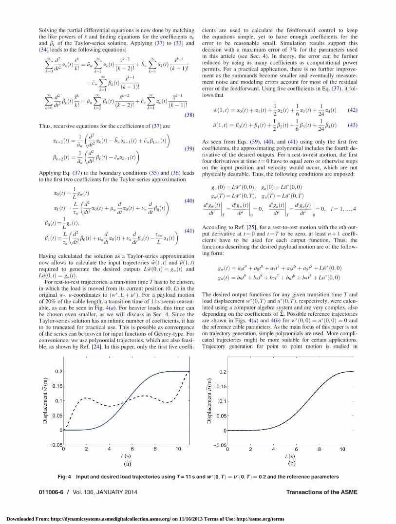
For rest-to-rest trajectories, a transition time T has to be chosen,in which the load is moved from its current position (0, L) in theoriginal w-, u-coordinates to ðw�; Lþ u�Þ. For a payload motionof 20% of the cable length, a transition time of 11 s seems reason-able, as can be seen in Fig. 4(a). For heavier loads, this time canbe chosen even smaller, as we will discuss in Sec. 4. Since theTaylor-series solution has an infinite number of coefficients, it hasto be truncated for practical use. This is possible as convergenceof the series can be proven for input functions of Gevrey-type. Forconvenience, we use polynomial trajectories, which are also feasi-ble, as shown by Ref. [24]. In this paper, only the first five coeffi-

cients are used to calculate the feedforward control to keepthe equations simple, yet to have enough coefficients for theerror to be reasonable small. Simulation results support thisdecision with a maximum error of 7% for the parameters usedin this article (see Sec. 4). In theory, the error can be furtherreduced by using as many coefficients as computational powerpermits. For a practical application, there is no further improve-ment as the summands become smaller and eventually measure-ment noise and modeling errors account for most of the residualerror of the feedforward. Using five coefficients in Eq. (37), it fol-lows that

�wð1; tÞ ¼ a0ðtÞ þ a1ðtÞ þ1

2a2ðtÞ þ

1

6a3ðtÞ þ

1

24a4ðtÞ (42)

�uð1; tÞ ¼ b0ðtÞ þ b1ðtÞ þ1

2b2ðtÞ þ

1

6b3ðtÞ þ

1

24b4ðtÞ (43)

As seen from Eqs. (39), (40), and (41) using only the first fivecoefficients, the approximating polynomial includes the fourth de-rivative of the desired outputs. For a rest-to-rest motion, the firstfour derivatives at time t¼ 0 have to equal zero or otherwise stepson the input position and velocity would occur, which are notphysically desirable. Thus, the following conditions are imposed:

gwð0Þ ¼ L �w�ð0;0Þ; guð0Þ ¼ L�u�ð0;0ÞgwðTÞ ¼ L �w�ð0;TÞ; guðTÞ ¼ L�u�ð0;TÞ

digwðtÞdti

��T

¼ digwðtÞdti

��0

¼ 0;diguðtÞ

dti

��T

¼ diguðtÞdti

��0

¼ 0; i¼ 1;…;4

According to Ref. [25], for a rest-to-rest motion with the nth out-put derivative at t¼ 0 and t¼T to be zero, at least nþ 1 coeffi-cients have to be used for each output function. Thus, thefunctions describing the desired payload motion are of the follow-ing form:

gwðtÞ ¼ a9t9 þ a8t8 þ a7t7 þ a6t6 þ a5t5 þ L �w�ð0; 0ÞguðtÞ ¼ b9t9 þ b8t8 þ b7t7 þ b6t6 þ b5t5 þ L�u�ð0; 0Þ

The desired output functions for any given transition time T andload displacement w�ð0;TÞ and u�ð0;TÞ, respectively, were calcu-lated using a computer algebra system and are very complex, alsodepending on the coefficients of ~R. Possible reference trajectoriesare shown in Figs. 4(a) and 4(b) for �w�ð0; 0Þ ¼ �u�ð0; 0Þ ¼ 0 andthe reference cable parameters. As the main focus of this paper is noton trajectory generation, simple polynomials are used. More compli-cated trajectories might be more suitable for certain applications.Trajectory generation for point to point motion is studied in

Fig. 4 Input and desired load trajectories using T 5 11 s and �w�ð0;T Þ ¼ �u�ð0;T Þ ¼ 0:2 and the reference parameters



Ref. [26], for example, including an arbitrary number of points inbetween that are to be passed within a specified safety corridor.

3.2 Feedback. A feedback law stabilizing Eqs. (22) and (23)is derived in this section. However, the feedback is designed fortwo uncoupled wave equations instead of the coupled equations.The uncoupled equations can be found in the literature describingthe orthogonal and tangential motion of a string, for example, inRef. [27]. The equations are derived by linearizing the nonlinearmodel around the steady states for F0 ¼ 0 and using 1þ e0ðxÞ � 1.Using this, the equations are found in a similar way as in Sec. 2.2.The orthogonal motion is governed by the PDE

@2 �w

@t2ð�x; tÞ ¼ ðbþ a�xÞ @

2 �w

@�x2ð�x; tÞ þ a

@ �w

@�xð�x; tÞ (44)

and the boundary conditions

@2 �w

@t2ð0; tÞ ¼ a

@ �w

@�xð0; tÞ

�wð1; tÞ ¼ 1

LUwðtÞ

(45)

using

a ¼ g

L; b ¼ mLg

mL2(46)

The tangential motion is governed in the domain by

@2 �u

@t2¼ EA

mL2

@2 �u

@�x2(47)

and at the boundaries by

@2 �u

@t2ð0; tÞ ¼ EA

mLL

@�u

@�xð0; tÞ

�uð1; tÞ ¼ 1

LUuðtÞ

(48)

Equation (44), along with the boundary conditions (45) canalso be found in Ref. [27]. Using this simplified cable model,the controller for each motion can be calculated separately.Note that the PDE describing the tangential motion is just aspecial case of the PDE describing the orthogonal motion inthe domain using a¼ 0 and b ¼ EA=mL2. The boundary con-ditions for both motions are equally structured as well. Dueto this fact, this paper will only focus on the design of theorthogonal controller and just state the calculated results forthe tangential controller at the end for completeness. Now,the transformation

vð�x; tÞ ¼ �wð�x; tÞ � �wð0; tÞ (49)

XðtÞ ¼ �wð0; tÞ; �wtð0; tÞð ÞT¼ X1ðtÞ;X2ðtÞð ÞT (50)

leads to the system

@2v

@t2ð�x; tÞ ¼ ðbþ a�xÞ @

2v

@�x2ð�x; tÞ þ a

@v

@�xð�x; tÞ � a

@v

@�xð0; tÞ (51)

with the boundary conditions

vð0; tÞ ¼ 0

vð1; tÞ ¼ VðtÞ ¼ 1

LUwðtÞ � X1ðtÞ

(52)

Here, X(t) is the state of the payload and has its own dynamics,which can be expressed in terms of a linear, time-invariant ODEgiven by

d

dtXðtÞ ¼ AXðtÞ þ

ffiffiffibp

B@v

@�xð0; tÞ (53)

with

A ¼0 1

0 0

� �

B ¼0affiffiffibp

! (54)

The transformation (49) can be seen as a moving coordinateframe. Whereas �wð�x; tÞ is the cable displacement relative to thez-axis in y-direction, vð�x; tÞ is the cable displacement relative tothe payload position X1ðtÞ, which is the center of the coordinateframe for vð�x; tÞ. This is illustrated in Fig. 5. Backstepping couldnow be applied to find a stabilizing controller. However, theresulting PDEs for the transformation kernels would be rather dif-ficult and could only be solved entirely by numerical implementa-tion, thus resulting in lower accuracy for the controller. In order toavoid these problems and to use backstepping similar to the waydescribed in Ref. [1] on the PDE-ODE cascade (51), (52) and(53), another transformation is introduced normalizing the wavepropagation speed to 1 and rescaling the PDE in space. This trans-formation is inspired by Refs. [28] and [4]. With

vð�x; tÞ ¼ffiffiffiffiffiffiffiffiffi2ffiffiffibpp

ffiffiffiffiffiffiffiffiffiffiffiffiffiffiffiffiffiffiffiazþ 2

ffiffiffibpp cðz; tÞ (55)

and

z ¼ gð�xÞ ¼ 2

aðffiffiffiffiffiffiffiffiffiffiffiffiffia�xþ bp

�ffiffiffibpÞ (56)

l ¼ gð1Þ ¼ 2

aðffiffiffiffiffiffiffiffiffiffiffiaþ bp

�ffiffiffibpÞ (57)

the transformed PDE-ODE cascade is given by

@2c

@t2ðz; tÞ ¼ @

2c

@z2ðz; tÞ þ bðzÞcðz; tÞ þ qðzÞ @c

@zð0; tÞ (58)

with

bðzÞ ¼ a2

4ðazþ 2ffiffiffibpÞ2

qðzÞ ¼ � affiffiffibp

ffiffiffiffiffiffiffiffiffiffiffiffiffiffiffiffiffiffiffiazþ 2

ffiffiffibp

2ffiffiffibp

s

and the boundary conditions are

Fig. 5 The different coordinate frames for describing themotion of the cable



cð0; tÞ ¼ 0

cðl; tÞ ¼ CðtÞ ¼ffiffiffiffiffiffiffiffiffiffiffiaþ b

b

4

rVðtÞ

(59)

For the payload dynamics, only the input has to be rescaled

d

dtXðtÞ ¼ AXðtÞ þ B

@c

@zð0; tÞ (60)

Now a backstepping controller combining ideas from Refs.[1,21,33] can be designed to stabilize the system around the ori-gin. We therefore introduce the transformation

qðz; tÞ ¼ hðzÞcðz; tÞ �ðz

0

kðz; yÞcðy; tÞdy�ðz

0

sðz; yÞ @c

@tðy; tÞdy

� cðzÞXðtÞ (61)

to map the system (58), (59), and (60) into the target system given by

@2q

@t2ðz; tÞ ¼ @

2q

@z2ðz; tÞ � 2d

@q

@tðz; tÞ � eqðz; tÞ (62)


qð0; tÞ ¼ 0

qðl; tÞ ¼ 0(63)

and the linear ODE

d

dtXðtÞ ¼ ðAþ BKÞXðtÞ þ B

@q

@zð0; tÞ (64)

The controller stabilizing Eqs. (58), (59), and (60) is then given by

CðtÞ ¼ 1

hðlÞ

ðl

0

kðl; yÞcðy; tÞdyþðl

0

sðl; yÞ @c

@tðy; tÞdyþ cðlÞXðtÞ

� �(65)

Substituting the time and space derivatives of Eq. (61) into the tar-get system (62) yields

0¼ @2q

@t2ðz; tÞ � @

2q

@z2ðz; tÞ þ 2d

@q

@tðz; tÞ þ eqðz; tÞ

¼ � 2dsðz; zÞ þ 2dh

dzðzÞ

� �@c

@zðz; tÞ

þ 2dhðzÞ þ 2@s

@zðz; zÞ þ 2

@s

@yðz; zÞ

� �@c

@tðz; tÞ

þ d2cz2ðzÞ � cðzÞA2 � 2dcðzÞA� ecðzÞ

� �XðtÞ

þ ehðzÞ � d2h

z2ðzÞ þ bðzÞhðzÞ þ 2

@k

@zðz; zÞ þ 2

@k

@yðz; zÞ

�

þ2d@s

@yðz; zÞ

�cðz; tÞ

þ sðz;0Þ �ðz

0

sðz;yÞqðyÞdy� cðzÞB� �

@2c

@t@zð0; tÞ

þ�

kðz;0Þ þ qðzÞhðzÞ �ðz

0

kðz;yÞqðyÞdy� cðzÞAB

þ 2d sðz;0Þ �ðz

0

sðz;yÞqðyÞdy� cðzÞB� ��

@czð0; tÞ

þðz

0

"@2k

@z2ðz;yÞ � @

2k

@y2ðz;yÞ � kðz;yÞbðyÞ � 2d

@2s

@y2ðz;yÞ

�2dbðyÞsðz;yÞ � ekðz;yÞ�

cðy; tÞdy

þðz

0

�@2s

@z2ðz;yÞ � @

2s

@y2ðz;yÞ�sðz;yÞbðyÞ

�2dkðz;yÞ � esðz;yÞ�@c

@tðy; tÞdy

For this equation to be zero for any point in space and time, eachcoefficient has to be equal to zero. Using this, along with theboundary condition of Eq. (62) at z¼ 0 and the ODE (64) andrewriting kzðz; zÞ þ kyðz; zÞ ¼ k0ðz; zÞ, the following equations forthe transformation kernels h(z), k(z, y), s(z, y) and cðzÞ are obtained:

@2k

@z2ðz; yÞ ¼ @

2k

@y2ðz; yÞ þ 2d

@2s

@y2ðz; yÞ þ 2dbðyÞsðz; yÞ

þ bðyÞ þ eð Þkðz; yÞ

kðz; 0Þ ¼ðz

0

kðz; yÞqðyÞdy� qðzÞhðzÞ þ cðzÞAB

2d

dzkðz; zÞð Þ ¼ d2h

dz2ðzÞ � bðzÞ þ eð ÞhðzÞ � 2d

@s

@yðz; zÞ

(66)

for k(z, y) and similar for s(z, y)

@2s

@z2ðz; yÞ ¼ @2s

@y2ðz; yÞ þ 2dkðz; yÞ þ bðyÞ þ eð Þsðz; yÞ

sðz; 0Þ ¼ðz

0

sðz; yÞqðyÞdyþ cðzÞB

sðz; zÞ ¼ � 1

d

dh

dzðzÞ

(67)

The boundary condition for cð0Þ can be found by using Eq. (61)for z¼ 0 along with the boundary condition q(0, t)¼ 0. This yieldscð0Þ ¼ 0. The boundary condition dh=dzð0Þ ¼ 0 can be obtainedby plugging z¼ 0 into the two last equations of Eq. (67). Usingc(0, t)¼ 0, h(0) can be chosen arbitrary. It can be regarded as akind of scaling factor, which is compensated for by the other ker-nel functions. To obtain the missing boundary conditiondc=dzð0Þ ¼ K, we need to differentiate Eq. (61) with respect to zand evaluate the result at z¼ 0. This yields

@q

@zð0; tÞ ¼ hð0Þ @c

@zð0; tÞ � dc

dzð0ÞXðtÞ

Thus, for the gain kernels h(z) and cðzÞ, the following equationsare obtained:

hðzÞ ¼ � 1

d

d

dzsðz; zÞð Þ (68)

with

hð0Þ ¼ 1

dh

dzð0Þ ¼ 0

(69)

and

d2cdz2ðzÞ ¼ cðzÞA2 þ 2dcðzÞAþ ecðzÞ (70)

cð0Þ ¼ ð0; 0ÞT

dcdzð0Þ ¼ K

(71)

Both functions h(z) and cðzÞ can be expressed in a closed form.This will make it easier to solve for k(z, y) and s(z, y) numerically.Thus, following the procedure in Ref. [4], h(z) can be calculatedanalytically by using Eqs. (67), (68), and (69). It follows that

hðzÞ ¼ coshðdzÞ (72)

From Eqs. (66) and (67), it can be found that s(0, 0)¼ 0 andkð0; 0Þ ¼ �qð0Þ has to hold. Now s(z, z) and k(z, z) can beobtained using h(z) in Eqs. (66) and (67), respectively. This yields



sðz; zÞ ¼ � sinhðdzÞ (73)

kðz;zÞ¼mðzÞ¼:dh

dzðzÞþ1

2hðzÞ

ðz

0

ðd2�bðyÞ�eÞdy�qð0Þ

¼ d sinhðdzÞþ1

2ðd2� eÞzcoshðdzÞþ1

2hðzÞ

ðz

0

bðyÞdy�qð0Þ

(74)

Equation (70) with the boundary conditions (71) can be solvedanalytically as well. For A as defined in Eq. (54), we obtain thefollowing solutions for cðzÞ:

cðzÞ¼

K1ffiffiffiep sinh

ffiffiffiep

z

K2ffiffiffiep sinh

ffiffiffiep

z�K1dffiffiffiffiffie3p sinh

ffiffiffiep

zþK1d

ezcosh

ffiffiffiep

z

0BBB@

1CCCA; e 6¼ 0

(75)

The limit value for cðzÞ as e! 0 does exist and is given by

cðzÞ ¼K1z

K1d

3z3 þ K2z

0@

1A; e ¼ 0 (76)

From this, we eventually obtain the kernel equations that have tobe solved numerically. Introducing the abbreviationkðyÞ ¼ bðyÞ þ e, we obtain for k(z, y)

@2k

@z2ðz; yÞ � @

2k

@y2ðz; yÞ ¼ 2d

@2s

@y2ðz; yÞ þ 2dbðyÞsðz; yÞ

þ kðyÞkðz; yÞ (77)

with

kðz; 0Þ ¼ðz

0

kðz; yÞqðyÞdy� qðzÞhðzÞ þ cðzÞAB

kðz; zÞ ¼ mðzÞ(78)

and for s(z, y)

@2s

@z2ðz; yÞ � @

2s

@y2ðz; yÞ ¼ 2dkðz; yÞ þ kðyÞsðz; yÞ (79)

with

sðz; 0Þ ¼ðz

0

sðz; yÞqðyÞdyþ cðzÞB;

sðz; zÞ ¼ � sinhðdzÞ(80)

The functions h(z) and cðzÞ are known from Eqs. (72), (75), and(76).

3.3 Existence of Solutions. In this section, we will prove theexistence of solutions to the PDEs satisfied by the kernels k(z, y)and s(z, y). This proof is inspired by Ref. [4], but modified due tothe boundary term in the domain of the original system (51), lead-ing to modified PDEs for the kernel compared with the system inRef. [4].

THEOREM 3.1 (Existence of solutions). Let q 2 C1ð½0; l�Þ andb 2 C0ð½0; l�Þ and d; c 2 C0ð½0; l�Þ. Then Eqs. (77) and (79) have aunique solution k; s 2 C2ð½0; l�Þ.

Proof. We use the method of successive approximations. Witha change of variables

n ¼ zþ y; g ¼ z� y (81)

the functions G ¼ Gðn; gÞ and Gs ¼ Gsðn; gÞ are defined as

Gðn; gÞ ¼ knþ g

2;n� g

2

� �; Gsðn; gÞ ¼ s

nþ g2

;n� g

2

� �

Let us also denote

g1ðnÞ :¼ mn2

� �; g2ðnÞ :¼ � sinh

dn2

� �(82)

b1 :¼ 2d; b2 :¼ kn� g

2

� �; b3 :¼ 2db

n� g2

� �(83)

For k(z, y) from Eq. (77), this change of variables yields

@2G

@n@gðn; gÞ ¼ 1

4b1

@2Gs

@n2ðn; gÞ � 2

@2Gs

@n@gðn; gÞ þ @

2Gs

@g2ðn; gÞ

� ��

þ b2Gðn; gÞ þ b3Gsðn; gÞ�

(84)

with

Gðn; 0Þ ¼ g1ðnÞ

Gðn; nÞ ¼ cðnÞAB�ðn

0

qðsÞGðn; sÞds� qðnÞhðnÞ(85)

and for s(z, y) from Eq. (79) we get

@2Gs

@n@gðn; gÞ ¼ 1

4b1Gðn; gÞ þ b2Gsðn; gÞð Þ (86)

with

Gsðn; 0Þ ¼ g2ðnÞ

Gsðn; nÞ ¼ cðnÞB�ðn

0

qðsÞGsðn; sÞds(87)

Integrating Eqs. (84) and (86) first with respect to g between 0 andg and then with respect to n from g to n and finally using theboundary conditions (85) and (87) yields

Gðn;gÞ ¼ cðgÞAB�ðg

0

qðsÞGðg;sÞds� qðgÞhðgÞþ g1ðnÞ� g1ðgÞ

þ 1

4

ðn

g

ðg

0

b2Gðs; sÞdsdsþ 1

4

ðn

g

ðg

0

b3Gsðs; sÞdsds

þ 1

4

ðn

g

ðg

0

b1

@2G

@n2ðs; sÞ� 2

@2G

@n@gðs; sÞþ @

2G

@g2ðs; sÞ

� �dsds

(88)

and

Gsðn; gÞ ¼ cðgÞB�ðg

0

qðsÞGsðg; sÞdsþ g2ðnÞ � g2ðgÞ

þ 1

4

ðn

g

ðg

0

b1Gðs; sÞdsdsþ 1

4

ðn

g

ðg

0

b2Gsðs; sÞdsds

(89)

From Eqs. (88) and (89), we find a solution by using a recursivemethod. We define the starting solutions G0ðn; gÞ and Gs;0ðn; gÞ as

G0ðn;gÞ¼ cðgÞAB�ðg

0

qðsÞG0ðg;sÞds�qðgÞhðgÞþg1ðnÞ�g1ðgÞ

(90)

Gs;0ðn; gÞ ¼ cðgÞB�ðg

0

qðsÞGs;0ðg; sÞdsþ g2ðnÞ � g2ðgÞ (91)

and the recursion for n¼ 0, 1, 2,…



Gnþ1ðn;gÞ¼1

4

ðn

g

ðg

0

b2Gnðs;sÞdsdsþ1

4

ðn

g

ðg

0

b3Gs;nðs;sÞdsds

þ1

4

ðn

g

ðg

0

b1

@2Gn

@n2ðs;sÞ�2

@2Gn

@n@gðs;sÞþ@

2Gn

@g2ðs;sÞ

� �dsds

(92)

Gs;nþ1ðn; gÞ ¼ 1

4

ðn

g

ðg

0

b1Gnðs; sÞdsdsþ 1

4

ðn

g

ðg

0

b2Gs;nðs; sÞdsds

(93)

The solution to Eqs. (84) and (86) is now given by

Gðn; gÞ ¼X1n¼0

Gnðn; gÞ; Gsðn; gÞ ¼X1n¼0

Gs;nðn; gÞ (94)

and is proven to exist in Ref. [4], presuming existence and bound-edness of G0ðn; gÞ and Gs;0ðn; gÞ. Those attributes are not obviousin our case and thus remain to be proven in a very similar wayusing proof by induction. Thus, we define a recursion with startingcondition

G0;0ðn; gÞ ¼ cðgÞAB� qðgÞhðgÞ þ g1ðnÞ � g1ðgÞ (95)

Gs;0;0ðn; gÞ ¼ cðgÞBþ g2ðnÞ � g2ðgÞ (96)

and the recursion formula

G0;nþ1ðn; gÞ ¼ �ðg

0

qðsÞG0;nðg; sÞds (97)

Gs;0;nþ1ðn; gÞ ¼ �ðg

0

qðsÞGs;0;nðg; sÞds (98)

Using

M :¼max jjcðgÞABjjL1ð0;lÞ þ jjqðgÞhðgÞjjL1ð0;lÞn

þ 2l

�� dg1

dnðnÞ��L1ð0;lÞ

; jjcðgÞBjjL1ð0;lÞ þ 2l

�� dg2


)

it can be concluded for the base case that

jG0;0ðn; gÞj � jcðgÞAB� qðgÞhðgÞ þ g1ðnÞ � g1ðgÞj

� jcðgÞABj þ jqðgÞhðgÞj þ jg1ðnÞ � g1ðgÞj

� jjcðgÞABjjL1ð0;lÞ þ jjqðgÞhðgÞjjL1ð0;lÞ

þ jj dg1

dnðnÞjjL1ð0;lÞjn� gj

� jjcðgÞABjjL1ð0;lÞ þ jjqðgÞhðgÞjjL1ð0;lÞ

þ 2l

�� dg1


� M

and similarly

jGs;0;0ðn; gÞj � jcðgÞBþ g2ðnÞ � g2ðgÞj� jcðgÞBj þ jg2ðnÞ � g2ðgÞj

� jjcðgÞBjjL1ð0;lÞ þ�� dg2


jn� gj

� jjcðgÞBjjL1ð0;lÞ þ 2l

�� dg2


� M

The induction hypothesis

jG0;nðn; gÞj � MKn ðnþ gÞn

n!(99)

jGs;0;nðn; gÞj � MKn ðnþ gÞn

n!(100)

holds for a particular, but unknown n 2N. Plugging Eq. (99) intoEq. (97) yields

jG0;nþ1ðn; gÞj ¼ðg

0

jqðsÞG0;nðg; sÞjds

�ðg

0

jqðsÞjMKn ðgþ sÞn

n!ds

�jjqjjL1ð0;lÞMKn

n!

ðg

0

ðgþ sÞnds


ðnþ 1Þ! ð2gÞnþ1 � gnþ1h i


ðnþ 1Þ! ðnþ gÞnþ1

and using the hypothesis (100) along with Eq. (98) it followssimilarly

jGs;0;nþ1ðn; gÞj ¼ðg

0

jqðsÞGs;0;nðg; sÞjds

�ðg

0

jqðsÞjMKn ðgþ sÞn

n!ds


n!

ðg

0

ðgþ sÞnds


ðnþ 1Þ! ð2gÞnþ1 � gnþ1h i


ðnþ 1Þ! ðnþ gÞnþ1

Thus, by induction it has been proven that Eq. (99) holds for alln 2N with K ¼ jjqjjL1ð0;lÞ, for example. This is bounded,because q is a continuous and differentiable function in a boundeddomain. Therefore, the solutions of Eqs. (90) and (91) exist andare given by the series

G0ðn; gÞ ¼X1n¼0

G0;nðn; gÞ; Gs;0ðn; gÞ ¼X1n¼0

Gs;0;nðn; gÞ (101)

From Eqs. (90) and (91) we can conclude that G0ðn; gÞ andGs;0ðn; gÞ belong to C2ð½0; l�Þ for a continuous and differentiableqðzÞ. Because Gðn; gÞ is defined on a bounded domain, this alsoimplies that jG0ðn; gÞj is bounded. Thus, existence and bounded-ness have been proven.

3.4 Inverse Transformation. To prove stability of theclosed-loop system, the inverse transformation has to exist andmust be unique. Let us define the inverse transformationqðz; tÞ ! cðz; tÞ as

cðz; tÞ ¼ lðzÞqðz; tÞ �ðz

0

mðz; yÞqðz; yÞdy�ðz

0

nðz; yÞ @q

@tðz; yÞdy

� aðzÞXðtÞ (102)

We can find the kernel equations in a very similar way as before.For the first term in Eq. (102), we obtain



lðzÞ ¼ 1

d

d

dzsðz; zÞ (103)


lð0Þ ¼ 1

dl

dzð0Þ ¼ 0

(104)

The kernel equations for m(z,y) in the second term of Eq. (102)become

@2m

@z2ðz; yÞ ¼ @

2m

@y2ðz; yÞ � 2d

@2n

@y2ðz; yÞ þ 2desðz; yÞ

� bðzÞ þ eð Þmðz; yÞ (105)


mðz; 0Þ ¼ qðzÞlð0Þ þ aðzÞABþ 2dnðz; 0

2d

dzmðz; zÞ ¼ d2l

dz2ðzÞ þ bðzÞ þ eð ÞlðzÞ þ 2d

@s

@yðz; zÞ

(106)

For the third term in (102) the equations are

@2n

@z2ðz; yÞ ¼ @

2n

@y2ðz; yÞ � 2dmðz; yÞ � bðzÞ � 4d2 � e

nðz; yÞ

(107)


nðz; 0Þ ¼ aðzÞB

nðz; zÞ ¼ 1

d

dl

dzðzÞ

(108)

For the kernel aðzÞ within the last term of Eq. (102) we obtain

d2adz2ðzÞ ¼ aðzÞA2 � bðzÞaðzÞ � qðzÞ dl

dzð0Þ (109)


að0Þ ¼ ð0; 0ÞT

dadzð0Þ ¼ �K

(110)

These equations are very similar to the equations satisfied by thekernels for the forward transformation. Thus, the existence of asolution for the kernels can be shown in a very similar way andthere exists a unique solution for l(z), aðzÞ, m(z, y), and n(z, y).

3.5 Stability of the Target System. For the target system,consisting of Eqs. (62), (63), and (64), we formulate the followingstability result.

THEOREM 3.2 (Stability of the closed-loop system). Consider theclosed-loop system consisting of the plant (58), (59), (60) and thecontrol law (65) with d > 0 and e > 0. Let k1 and k2 denote thetwo eigenvalues of the matrix AþBK and let K be chosensuch that both eigenvalues have negative real parts. Then allthe eigenvalues of the closed-loop system have negative realparts and reside to the left of the vertical lineReðkÞ ¼ maxfReðk1Þ;Reðk2Þ;�d;Reð�d þ

ffiffiffiffiffiffiffiffiffiffiffiffiffid2 � ep

Þg.Proof. We investigate the spectrum of the target system (62),

(63), (64), because the target system and the closed-loop system,(58), (59), (60), (65) in the original variables have the same spec-

trum. For determining the spectrum of the target system, we seeka solution of the form

qðz; tÞ ¼ expðrtÞuðzÞ (111)

Substituting this into Eq. (62) yields

r2uðzÞ ¼ d2

dz2uðzÞ � 2druðzÞ � euðzÞ

) 0 ¼ d2

dz2uðzÞ � ð2drþ eþ r2ÞuðzÞ (112)

with the appropriate boundary conditions

uð0Þ ¼ 0 (113)

uðlÞ ¼ 0 (114)

The solution to this boundary value problem using Eqs. (112) and(113) is given by

uðzÞ ¼ C sinh zffiffiffiffiffiffiffiffiffiffiffiffiffiffiffiffiffiffiffiffiffiffiffiffiffiffiffi2drþ eþ r2

p� �(115)

From boundary condition (114), r can be calculated as

lffiffiffiffiffiffiffiffiffiffiffiffiffiffiffiffiffiffiffiffiffiffiffiffiffiffiffi2drþ eþ r2

p¼ ikp

) rð2k�1Þ=ð2kÞ ¼ �d6

ffiffiffiffiffiffiffiffiffiffiffiffiffiffiffiffiffiffiffiffiffiffiffiffiffiffiffiffiffiffiffiffiffid2 � e� kp

l

� �2s

; k 2N=0 (116)

Thus, for any choice of d > 0 and e > 0, the eigenvalues reside inthe left half of the complex plane and in fact the rightmost eigen-value is always left of or on the vertical line at kmax, with

kmax ¼ maxð�d;Reð�d þffiffiffiffiffiffiffiffiffiffiffiffiffid2 � ep

ÞÞ (117)

Note, that for e d2, all eigenvalues have the same real part, withReðrkÞ ¼ �d. Including the two eigenvalues from AþBK intothe spectrum gives the result stated in the theorem above.

From this analysis, it can be seen that the closed-loop systemsatisfying the compatibility condition

cðl;0Þ¼ 1

hðlÞ

ðl

0

kðl;yÞcðy;0Þdyþðl

0

sðl;yÞ@c

@tðy;0Þdyþ cðlÞXð0Þ

� �(118)

is asymptotically stabilized by the control law (65). Transforming(65) back into the original variables yields the controller

1

LUwðtÞ ¼ �wð0; tÞ þ

ffiffiffiffiffiffiffiffiffiffiffib

aþ b

4

r "ð1

0

kð1; yÞf ðyÞð�wðy; tÞ � �wð0; tÞÞdy

þð1

0

sð1; yÞf ðyÞ @ �w

@tðy; tÞ � @ �w

@tð0; tÞ

� �dy

þ cð1Þð�wð0; tÞ; @ �w

@tð0; tÞÞT

#(119)

with

f ðyÞ ¼ ½b ayþ bð Þ��14 (120)

which drives the system (44) and (45) to �wð�x; tÞ ¼ 0 for �x 2 ½0; 1�and t 2 ½0;1Þ. For a given desired trajectory w�ðx; tÞ the control-ler with



Fig. 6 Comparing the actual w(L, t) (dotted) and desired w*(L, t) (solid) payload motion. The input w(0, t) (dashed) is alsoshown. The transition time is T 5 15 s.

Fig. 7 Spatially varying weighing terms for position and velocity feedback for L 5 100 m (solid) and L 5 200 m (dashed)

Fig. 8 Closed-loop simulation results for an orthogonal and tangential displacement of 20 m. The transition time is T 5 15 s.The desired trajectory (solid) and the actual trajectory (dotted) are with the left axis, the difference (dash-dotted) is shown onthe right axis. Note that two different y-scales have been used to magnify the error.



Fig. 9 Closed-loop simulation results for an orthogonal and tangential displacement of 20 m. The transition time is T 5 15 s.The feedforward control input (solid) is with the left axis, the feedback part (dash-dotted) is shown on the right axis. Note thattwo different y-scales have been used to magnify the feedback part.

Fig. 10 Closed-loop simulation results for an orthogonal and tangential displacement of 20 m. The transition time is T 5 30 s.The desired trajectory (solid) and the actual trajectory (dotted) are with the left axis, the difference (dash-dotted) is shown onthe right axis. Note that two different y-scales have been used to magnify the error.

Fig. 11 Closed-loop simulation results for a step-shaped disturbance from t 5 10 s to t 5 35 s. The desired trajectory (solid) andthe actual trajectory (dotted) are with the left axis, the difference (dash-dotted) is shown on the right axis. Note that two differenty-scales have been used to magnify the error.



UwðtÞ ¼ wð0; tÞ � w�ð0; tÞ

þffiffiffiffiffiffiffiffiffiffiffi

b

aþ b

4

r �ð1

0

kð1; yÞf ðyÞ�

wðLy; tÞ � w�ðLy; tÞ � wð0; tÞ

þ w�ð0; tÞ�

dy

þð1

0

sð1; yÞf ðyÞ�@w

@tðLy; tÞ � @w�

@tðLy; tÞ � @w

@tð0; tÞ

þ @w�

@tð0; tÞ

�dy

þ cð1Þ wð0; tÞ � w�ð0; tÞ; @w

@tð0; tÞ � @w�

@tð0; tÞ

� �T�(121)

achieves limt!1 w�ðx; tÞ � wðx; tÞ ¼ 0. This result can be foundby designing the controller not for the original system, but for theerror system using ewðx; tÞ ¼ wðx; tÞ � w�ðx; tÞ assuming thedesired trajectory w�ðx; tÞ fulfills the original system equations(44) and (45). The desired trajectory has to comply with the com-patibility condition (119). A trajectory fulfilling

w�ðx; 0Þ ¼ 0 and@w�

@tðx; 0Þ ¼ 0 (122)

will always meet this requirement, as do the trajectories describedin Sec. 3.1. The controller for the tangential motion with the gainkernels calculated accordingly is given by

UuðtÞ ¼ uð0; tÞ � u�ð0; tÞ þð1

0

kð1; yÞ 1ffiffiffibp ðuðLy; tÞ � u�ðLy; tÞ

� uð0; tÞ þ u�ð0; tÞÞdy

þð1

0

sð1; yÞ 1ffiffiffibp�@u

@tðLy; tÞ � @u�

@tðLy; tÞ � @u

@tð0; tÞ

þ @u�

@tð0; tÞÞdyþ cð1Þðuð0; tÞ � u�ð0; tÞ; @u

@tð0; tÞ

� @u�

@tð0; tÞ

�T

(123)

4 Results

The simulation results shown in this section have been obtainedfor a steel cable of length L¼ 100 m and a specific mass ofm ¼ 8:95 kg=m. The used payload mass is mL ¼ 1000 kg, whichis actually at the lower end of possible payload masses for thisapplication. The controller can be chosen even faster for highermasses. The performance of the open loop with feedforward con-trol can be seen in Fig. 6 for a transition time of T¼ 15 s. Afterstopping at the desired position, the payload keeps oscillatingaround it with a small amplitude due to the cut-off of the Taylor-series approximation. Therefore, the feedback loop is used to min-imize these errors. For the same cable parameters as above, Fig. 7shows the numerical solution for k(1, y) and s(1, y) for two differ-ent cable lengths. The results are shown in Fig. 8 for the sametransition time of T¼ 15 s. The different contributions of the feed-forward and the feedback part are shown in Fig. 9. It can be seenthat the feedforward accounts for most of the input during thetransition time, while the feedback part remains below 5% of theoverall control input. Due to the slower motion and thus smallerhigher derivatives, for a longer transition time of T¼ 30 s theresults are even better, as can be seen in Fig. 10. In Fig. 11, thecable is initially at rest and after t¼ 10 s subject to a step shapeddisturbance. The stream velocity is increased by 0:5 m=s, whichintroduces an additional force to the payload leading to a constantoffset, due to the P-feedback structure of the controller with no in-

tegral part. At t¼ 35 s, the disturbance is switched off and theclosed-loop error goes back to wðL; tÞ � w�ðL; tÞ ¼ 0 anduðL; tÞ � u�ðL; tÞ ¼ 0.

5 Conclusion

This paper presents the design of an asymptotically stabilizingcontroller for a coupled wave equation system in one spatialdimension. The partial differential equations used to calculate thegain kernels are derived analytically and solved numerically. Theclosed-loop spectrum resides entirely in the left half of the com-plex plane. A larger mass and a shorter cable contribute to a bettercontroller performance. The reason for this can be found by look-ing at the feedforward design. Since the coefficients are assumedto be constant in the design approach, the accuracy dependsmostly on the deviation of the coefficients relative to the meanvalue. For each coefficient, this deviation is somewhat determinedby the cable mass compared with the payload mass. Thus, for ashorter cable and a heavier payload, the feedforward gives moreaccurate results than for a longer cable or a lighter payload. Addi-tionally, the accuracy can be further improved using longer transi-tion times, which is physically suitable, as there are simplyphysical limits to moving a huge payload with a mass of morethan 1000 kg from one point to another. Using more coefficientsof the Taylor-series solution for the feedforward controller elimi-nates this problem in principle, but other problems arise frominput bounds. The feedback controller was designed for adecoupled, hence simpler model. As could be seen from the simu-lation, it can be used as a stabilizing feedback along with the feed-forward controller for the coupled equations and the results werevery good, with only small errors.

For a practical implementation of the presented controlapproach, two points have to be considered. First, actuator limitshave to be taken into account. For a very fast controller, velocity,and acceleration at the top can easily exceed these limits. Thus,the controller has to be tuned according to the dynamics of theavailable actuators. Second, because the infinite dimensionalstates u(x, t), utðx; tÞ, w(x, t), and wtðx; tÞ can never be measuredentirely, it is always necessary to design an observer in order toimplement such a backstepping controller. Observer design hasnot been subject of this paper, but it is very similar to the designof the controller itself and is subject of ongoing research. Care hasto be taken in where to place sensors and what to measure. From atheoretical point of view, measuring the position of the payloadwould be best. In order to stabilize the observer system, an addi-tional measurement either at the input boundary or anywhere atthe cable is also necessary. Unfortunately, implementing a posi-tion measurement for the cable can be difficult in practice. Thus,acceleration measurements taken at the payload position and eval-uated according to Refs. [29–31] are a possibility. Further infor-mation on observer design for linear PDEs and PDE-ODEcascades using backstepping techniques is provided by Refs.[1,21], for example.

Acknowledgment

This work was mostly done during a stay of the correspondingauthor at the University of California, San Diego. Thanks are dueto the German Academic Exchange Service for funding the stayand thus making this work possible.

References[1] Krstic, M., 2009, Delay Compensation for Nonlinear, Adaptive, and PDE Sys-

tems, Birkhauser, Boston, MA.[2] Wang, J.-M., Guo, B.-Z., and Krstic, M., 2011, “Wave Equation Stabilization

by Delays Equal to Even Multiples of the Wave Propagation Time,” SIAM J.Control Optim., 49, pp. 517–554.

[3] Gerdts, M., Greif, G., and Pesch, H. J., 2008, “Numerical Optimal Control ofthe Wave Equation: Optimal Boundary Control of a String to Rest in FiniteTime,” Math. Comput. Simul., 79, pp. 1020–1032.



http://dx.doi.org/10.1137/100796261

http://dx.doi.org/10.1137/100796261

http://dx.doi.org/10.1016/j.matcom.2008.02.014

[4] Smyshlyaev, A., Cerpa, E., and Krstic, M., 2010, “Boundary Stabilization of a1-D Wave Equation With In-Domain Antidamping,” SIAM J. Control Optim.,48, pp. 4014–4031.

[5] Wagner, M. O., Meurer, T., and Kugi, A., 2009, “Feedforward Control Designfor a Semilinear Wave Equation,” Proc. Appl. Math. Mech., 9(1), pp. 7–10.

[6] Meurer, T., and Kugi, A., 2011, “Tracking Control Design for a Wave EquationWith Dynamic Boundary Conditions Modeling a Piezoelectric Stack Actuator,”Int. J. Robust Nonlinear Control, 21(5), pp. 542–562.

[7] Ge, S. S., He, W., How, B., and Choo, Y. S., 2010, “Boundary Control of aCoupled Nonlinear Flexible Marine Riser,” IEEE Trans. Control Syst. Technol.,18(5), pp. 1080–1091.

[8] He, W., Ge, S. S., Hang, C. C., and Hong, K.-S., 2010, “Boundary Control of aVibrating String Under Unknown Time-Varying Disturbance,” 49th IEEE Con-ference on Decision and Control (CDC), pp. 2584–2589.

[9] Chen, L.-Q., 2005, “Analysis and Control of Transverse Vibrations of AxiallyMoving Strings,” Appl. Mech. Rev., 58, pp. 91–116.

[10] Wang, J., and Li, Q., 2004, “Active Vibration Control Methods of Axially Mov-ing Materials—A Review,” J. Vib. Control, 10(4), pp. 475–491.

[11] Nguyen, T., and Egeland, O., 2004, “Stabilization of Towed Cables,” 43rdIEEE Conference on Decision and Control, CDC, Vol. 5, pp. 5059–5064.

[12] Nguyen, T. D., and Egeland, O., 2004, “Observer Design for a Towed Seismic Cable,”Proceedings of the American Control Conference, Vol. 3, pp. 2233–2238.

[13] How, B., Ge, S. S., and Choo, Y. S., 2011, “Control of Coupled Vessel, Crane,Cable, and Payload Dynamics for Subsea Installation Operations,” IEEE Trans.Control Syst. Technol., 19(1), pp. 208–220.

[14] Krstic, M., 2009, “Compensating a String PDE in the Actuation or Sensing Pathof an Unstable ODE,” IEEE Trans. Autom. Control, 54(6), pp. 1362–1368.

[15] Nestegard, and Bone, 2008, Modelling and Analysis of Marine Operations, DetNorske Veritas, Hovik, Norway, No. DNV-RP-H103.

[16] Newman, J. N., 1977, Marine Hydrodynamics, The MIT Press, Cambridge, MA.[17] Triantafyllou, M. S., 1984, “The Dynamics of Taut Inclined Cables,” Q. J.

Mech. Appl. Math., 37, pp. 421–440.[18] Burgess, J. J., and Triantafyllou, M. S., 1988, “The Elastic Frequencies of

Cables,” J. Sound Vib., 120(1), pp. 153–165.[19] Papazoglou, V. J., Mavrakos, S. A., and Triantafyllou, M. S., 1990, “Non-Linear

Cable Response and Model Testing in Water,” J. Sound Vib., 140(1), pp. 103–115.[20] Ugural, A. C., and Fenster, S. K., 1975, Advanced Strength and Applied Elastic-

ity, American Elsevier Publishing Company, New York.

[21] Krstic, M., and Smyshlyaev, A., 2008, Boundary Control of PDEs: A Courseon Backstepping Designs, Society for Industrial and Applied Mathematics, Phil-adelphia, PA.

[22] Kharitonov, A., and Sawodny, O., 2006, “Flatness-Based Feedforward Controlfor Parabolic Distributed Parameter Systems With Distributed Control,” Int. J.Control, 79(7), pp. 677–687.

[23] Lynch, A. F., and Rudolph, J., 2002, “Flatness-Based Boundary Control of aClass of Quasilinear Parabolic Distributed Parameter Systems,” Int. J. Control,75(15), pp. 1219–1230.

[24] Rudolph, J., and Woittennek, F., 2006, “Trajektorienplanung fur die Steuerunggewisser linearer Systeme mit verteilten Parametern (Trajectory Planning forthe Control of some Linear Distributed Parameter Systems),” Automatisierung-stechnik, 54, pp. 228–239.

[25] Craig, J. J., 1989, Introduction to Robotics: Mechanics and Control, 2nd ed.,Addison-Wesley Longman Publishing Co., Inc., Boston, MA.

[26] Ruppel, T., Zimmert, N., Zimmermann, J., and Sawodny, O., 2008,“Kinodynamic Planning—An Analytical Approximation With Cn Polynomialsfor Industrial Application,” IEEE International Conference on Control Applica-tions, CCA, pp. 528–533.

[27] Petit, N., and Rouchon, P., 2001, “Flatness of Heavy Chain Systems,” ControlOptim., 40, pp. 475–495.

[28] Zhao, S., and Xie, C., 2010, “Output-Feedback Stabilization of the Wave Equa-tion With Spatially Varying Propagation Speed,” 49th IEEE Conference on De-cision and Control.

[29] Kuchler, S., Mahl, T., Neupert, J., Schneider, K., and Sawodny, O., 2011,“Active Control for an Offshore Crane Using Prediction of the Vessel’sMotion,” IEEE/ASME Trans. Mechatron., 16(2), pp. 297–309.

[30] Kuchler, S., Eberharter, J. K., Langer, K., Schneider, K., and Sawodny, O.,2011, “Heave Motion Estimation of a Vessel Using Accelerometer Meas-urements,” 18th IFAC World Congress, pp. 14742–14747.

[31] Kuchler, S., Pregizer, C., Eberharter, J. K., Schneider, K., and Sawodny, O.,2011, “Real-Time Estimation of a Ship’s Attitude,” American Control Confer-ence (ACC), pp. 2411–2416.

[32] Smyshlyaev, A., and Krstic, M., 2009, “Boundary Control of an Anti-StableWave Equation With Anti-Damping on the Uncontrolled Boundary,” Syst. Con-trol Lett., 58, pp. 617–623.

[33] Susto, G. A., and Krstic, M., 2010, “Control of PDE-ODE Cascades With Neu-mann Interconnections,” J. Franklin Inst., 347(1), pp. 284–314.



http://dx.doi.org/10.1137/080742646

http://dx.doi.org/10.1002/pamm.200910003

http://dx.doi.org/10.1002/rnc.1611

http://dx.doi.org/10.1109/TCST.2009.2033574

http://dx.doi.org/10.1115/1.1849169

http://dx.doi.org/10.1177/1077546304035605



http://dx.doi.org/10.1109/TAC.2009.2015557

http://dx.doi.org/10.1093/qjmam/37.3.421

http://dx.doi.org/10.1093/qjmam/37.3.421

http://dx.doi.org/10.1016/0022-460X(88)90340-9

http://dx.doi.org/10.1016/0022-460X(90)90909-J

http://dx.doi.org/10.1080/00207170600622858

http://dx.doi.org/10.1080/00207170600622858

http://dx.doi.org/10.1080/00207170210163640

http://dx.doi.org/10.1524/auto.2006.54.5.228

http://dx.doi.org/10.1524/auto.2006.54.5.228

http://dx.doi.org/10.1137/S0363012900368636

http://dx.doi.org/10.1137/S0363012900368636

http://dx.doi.org/10.1109/TMECH.2010.2041933

http://dx.doi.org/10.1016/j.sysconle.2009.04.005

http://dx.doi.org/10.1016/j.sysconle.2009.04.005

http://dx.doi.org/10.1016/j.jfranklin.2009.09.005

michael bo¨hm modeling and boundary control

Documents