-

NOAA Technical Memorandum ERL PMEL-20

METLIB - A PROGRAM LIBRARY FOR CALCULATING

AND PLOTTING MARINE BOUNDARY LAYER WIND FIELDS

J. E. OverlandR. A. BrownC. D. Mobley

Pacific Marine Environmental LaboratorySeattle, WashingtonJune 1980

UNITED STATESDEPARTMENT OF COMMERCEPhilip M. Klutznick, Secretlry

NATIONAL OCEANIC AND

ATMOSPHERIC ADMINISTRATION

Richard A. Frank, Administrator

Environmental Research

Laboratories

Wilmot N. Hess. Director

NOTICE

The Environmental Research Laboratories do not approve,recommend, or endorse any proprietary product or proprietarymaterial mentioned in this publication. No reference shallbe made to the Environmental Research Laboratories or to thispublication furnished by the Environmental Research Labora­tories in any advertising or sales promotion which would in­dicate or imply that the Environmental Research Laboratoriesapprove, recommend, or endorse any propri etary product orproprietary material mentioned herein, or which has as itspurpose an intent to cause directly or indirectly the adver­tised product to be used or purchased because of this Envi­ronmental Research Laboratories publication.

i i

CONTENTS

Page

Abstract 1

1. INTRODUCTION 1

2. DATA SOURCES 2

3. DATA MANAGEMENT 3

4. MAIN PROGRAMS 8

4.1 Use of METLIB 8

4.2 UNPACK (Used to Extract Subsets from Large Temporal or

Geographic Data Sets Such as NCAR) 8

4.3 DECKS (Creates a Standard Format File from Digitized Fields) 9

4.4 WINDS (CalCUlations of Winds) 10

4.5 PTWND (Time Series of Winds) 12

4.6 PLOTGRD (Plotting) 13

4.7 MAP (Plotting Map Backgrounds) 21

4.8 PLOTW.PLOT2W.PLOT2W2 (Combined Submit Files) 22

5. SUBROUTINE DOCUMENTATION 26

5.1 IntrOduction 26

5.2 Interpolation (NTERP) 26

5.3 Location on Subgrid (W3FBOO.W3FB01) 26

5.4 Speed and Direction (W3FC02.W3FCOO) 28

5.5 Thermal Wind (TMWND) 28

5.6 GRIDSET (GRIDSET) 28

5.7 Geostrophic Wind (GEOWIN.EDGE) 29

5.8 Gradient Wind (GRDWD) 29

5.9 Empirical Constants (MODEL4) 29

5.10 Model 2 (MODEL2) 29

5.11 Models 6-8 (MODEL6.MODEL8.BROWN.CARDON. etc) 30

6. ACKNOWLEDGEMENTS 31

7. REFERENCES 32

APPENDIX A: DERIVATION OF THE UNIVERSITY OF WASHINGTON (BROWN)

PLANETARY BOUNDARY LAYER MODEL 33

APPENDIX B: DERIVATION OF CARDONE MODEL 67

iii

METLIB - A PROGRAM LIBRARY FOR CALCULATING AND PLOTTINGMARINE BOUNDARY LAYER WIND FIELDS*

J. E. OverlandPacific Marine Environmental Laboratory

Seattle. Washington

R. A. BrownC. D. Mobley

University of WashingtonSeattle. Washington

METLIB is a FORTRAN program library for deriving earth-located

time series of geostrophic. gradient. or surface winds from sea

level pressure (SLP) and ancillary fields gridded on a polar

stereographic projection. Such fields are generated at the National

Meteorological Center (NMC) and at Fleet Numerical Oceanographic

Central (FNOC). They can also be generated by digitizing SLP

charts analyzed manually. The library also contains programs for

contouring scalars. such as SLP or wind speed. and for plotting

vector arrows with a map background. Plotting is based upon the

NCAR graphics routines. A major advantage to the library is that

spherical geometric calculations involving polar stereographic

grids are internal to the programs. The relationship between

gradient wind and surface wind can be assigned from speed reduction

and turning angle constants or by a baroc1inic. stability-dependent.

single point boundary layer model.

1. INTRODUCTION

This document provides an introduction to the program library. dis­

cusses the data structure used by the library. and provides documentation

of the geophysical algorithms used to derive various parameters and perform

geometric calculations. It provides a description of the SUBMIT files for

accessing the library as of date of publication. The library is divided

into four program divisions. UNPACK or DECKS. WINDS. PTWIND. and PLOTGRD

and two subroutine libraries. WSUBLIB and those called by PLTPROC.

*Contribution No. 451 from NOAA/ERL Pacific Marine Environmental Laboratory.

UNPACK extracts data from a larger data set, normally tapes such as

those supplied by NCAR or NMC, and creates a master file in a standard format

for all subsequent programs. DECKS performs the same function as UNPACK for

card or terminal input of fields that have been digitized from manual

analyses. Program WINDS inputs a series of sea-level pressure (SLP) fields

in standard format and, depending upon the option, can also input air

temperature, air-sea temperature difference and dew point depression fields.

It outputs u and v components at each grid point. Output winds can be

geostrophic, gradient. empirical reduction and turning of the gradient wind,

or calculated from a planetary boundary layer (PBL) model. Two of the three

PBL models have the option of outputing stress or heat flux in place of

surface wind. PTWIND can take u and v fields generated by WINDS, interpolate

them to any specified latitude and longitude, and convert the grid compo­

nents to speed and direction relative to north. PLOTGRD can input and

contour up to two scalar fields and can plot their difference. It can draw

arrow plots of a vector field or the difference of two vector fields, and

can plot a vector field with contours of a scalar, including contours of the

magnitude (isotachs) of the vector field itself or the difference in magni­

tude of two vector fields. All routines are intended to be machine­

independent FORTRAN programs.

For use at PMEL or other locations with access to the Environmental

Research Laboratories· CDC 6600 computer in Boulder, Colorado, SUBMIT files

are shown for WINDS, PLOTGRD and their combination. These SUBMIT files are

specific to the NOS 1.3 operating system in use at the time of publica­

tion. RWINDS submits WINDS and RPLOT submits PLOTGRD. PLOTW inputs scalar

fields, calculates wind fields and plots the results (i.e., runs WINDS and

PLOTGRD together). PLOT2W inputs scalars, runs WINDS twice, and plots

vector differences. PLOT2W2 inputs two separate sets of SLP scalars,

calculates winds for each and plots their difference.

2. DATA SOURCES

NMC currently produces SLP and surface air temperature (SAT) analyses

at 0000 and 1200 GMT on one of two polar stereographic meshes: the PE 65 x

65 point grid, with a spacing of 381 km at 600 N covering the northern

2

hemisphere; and the LFM 53 x 57 point grid. a fine-mesh grid with a spacing

of 190.5 km at 60o N, covering North America and the adjacent waters (Fig. 1

and 2). PE and LFM are historical names standing for Ilfrimitive ,Equation ll

and IIbimited Area fine-Mesh Model li• The PE data are archived at the

National Center for Atmospheric Research (NCAR) (Jenne. 1975) and the

National Climate Center (NCC). At present the LFM data are not routinely

archived for general distribution. Pressure fields are also produced by

Fleet Numerical Oceanographic Central (FNOC) on a 63 x 63 point grid with

the same scale and orientation as the PE grid. All grids are uniformly

spaced upon a polar stereographic map projection. which preserves angles.

Over the ocean, SLP and SAT values for operational forecast models are

obtained from ocean-station vessel, bUoy and ship observations analysed by a

variety of objective analysis techniques (Cressman. 1959; Flattery, 1970;

Holl and Mendenhall. 1971). For many research purposes it is necessary to

reanalyze the SLP charts making use of reports that were not included in the

NMC analysis. To this end, the reanalysis is done on a standard polar

stereographic projection (either the PE or LFM) and digitized at a uniform

spacing compatible with the program library.

Internal north-pole coordinates are (33,33) for the present PE grid and

(27,49) for the LFM. The FNOC pressure fields use pole coordinates of

(32.32). For PE data prior to 1976 the NMC Il octagon ll was used. The number

of grid points was 47 x 51, the pole location was (24,26), and the data were

stored in a one-dimensional array. This is the format used by NCAR to store

much of their NMC PE data.

3. DATA MANAGEMENT

All master data files created by UNPACK or DECKS are in a standard

format for subsequent analysis routines. Master data sets are arranged

chronologically and separated by type (e.g., SLP or wind speed) and geo­

graphical region (e.g., the Gulf of Alaska). Thus, one file might have a

1-yr time series of observed SLP's in a 10 x 10 grid for the Gulf of Mexico;

another file might consist of model-generated, u-component winds for the

same period. etc.

3

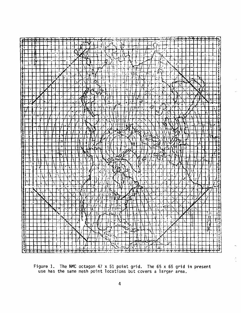
Figure 1. The NMC octagon 47 x 51 point grid. The 65 x 65 grid in presentuse has the same mesh point locations but covers a larger area.

4

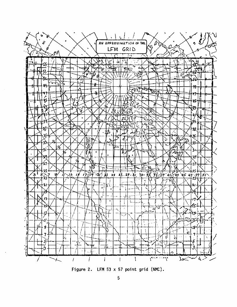
Figure 2. LFM 53 x 57 point grid (NMC).

5

IFACT =

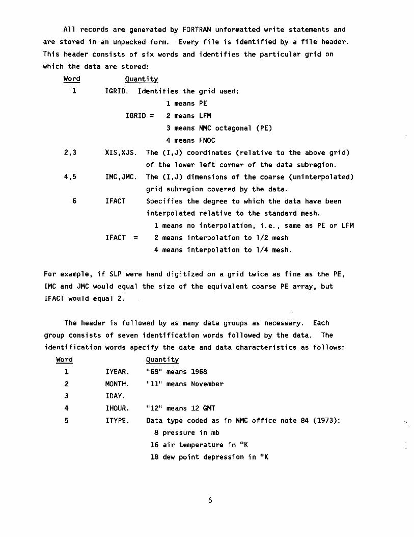
All records are generated by FORTRAN unformatted write statements and

are stored in an unpacked form. Every file is identified by a file header.

This header consists of six words and identifies the particular grid on

which the data are stored:

Word Quantity

1 IGRID. Identifies the grid used:

1 means PE

IGRID = 2 means LFM

3 means NMC octagonal (PE)

4 means FNOC

2,3 XIS,XJS. The (I,J) coordinates (relative to the above grid)

of the lower left corner of the data subregion.

4,5 IMC,JMC. The (I,J) dimensions of the coarse (uninterpo1ated)

grid subregion covered by the data.

6 IFACT Specifies the degree to which the data have been

interpolated relative to the standard mesh.

1 means no interpolation, i.e., same as PE or LFM

2 means interpolation to 1/2 mesh

4 means interpolation to 1/4 mesh.

For example, if SLP were hand digitized on a grid twice as fine as the PE,

IMC and JMC would equal the size of the equivalent coarse PE array, but

IFACT would equal 2.

The header is followed by as many data groups as necessary. Each

group consists of seven identification words followed by the data. The

identification words specify the date and data characteristics as follows:

Word Quantity

1 IYEAR. 116811 means 1968

2 MONTH. 111111 means November

3 IDAY.

4 IHOllR. 1112" means 12 GMT

5 ITYPE. Data type coded as in NMC office note 84 (1973):

8 pressure in mb

16 air temperature in oK

18 dew point depression in oK

6

means 12-hr forecast data

means 24-hr forecast data, etc.

means climate type 1.0

means climate type 2.0, etc.

6

7

lOBS.

lOBS =

IFLAG.

IFLAG =

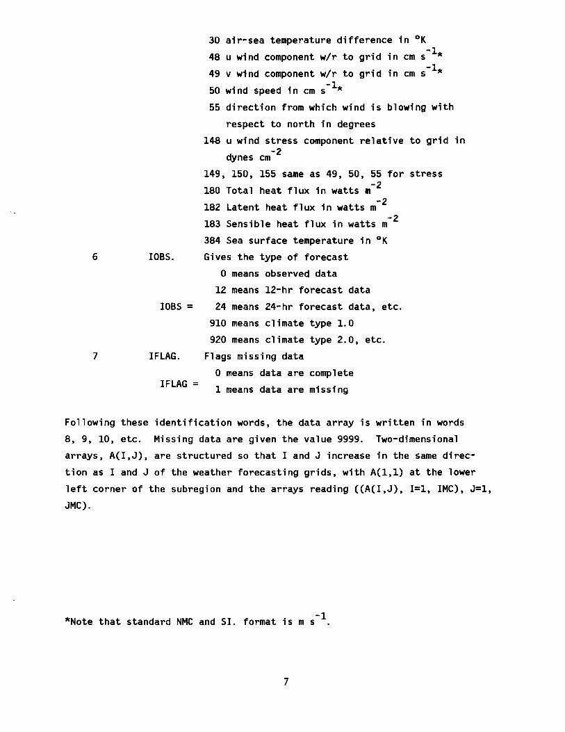
30 air-sea temperature difference in oK

48 u wind component w/r to grid in cm s-l*

49 v wind component w/r to grid in cm 5-1*

-150 wind speed in cm s *

55 direction from which wind is blowing with

respect to north in degrees

148 u wind stress component relative to grid in-2dynes cm

149, ISO, 155 same as 49, 50, 55 for stress

180 Total heat flux in watts m- 2

182 Latent heat flux in watts m- 2

183 Sensible heat flux in watts m- 2

384 Sea surface temperature in oK

Gives the type of forecast

o means observed data

12

24

910

920

Flags missing data

o means data are complete

1 means data are missing

Following these identification words, the data array is written in words

8, 9, 10, etc. Missing data are given the value 9999. Two-dimensional

arrays, A(I,J), are structured so that I and J increase in the same direc­

tion as I and J of the weather forecasting grids, with A(l,l) at the lower

left corner of the subregion and the arrays reading ((A(I,J), 1=1, IMC), J=l,

JMC).

*Note that standard NMC and 51. format is m s-l

7

4. MAIN PROGRAMS

4.1 Use of MEllIS

METlIB consists of a collection of programs and subroutines along with

a set of SUBMIT files to run them. These libraries and example files are

stored under USER. MEllIB on the ERl 6600 computer. This USER is meant for

read-only storage of programs. All data files and personal copies of SUBMIT

and main program files should be stored in separate USER areas. Normal pro­

cedure is to copy the desired files from METlIB into a new area and then

modify the files as necessary for a particular application. This entails

changing the SUBMIT files and the dimension statements of the main programs

to match the data array size.

4.2 UNPACK (Used to Extract Subsets from large

Temporal or Geographic Data Sets such as NCAR)

UNPACK performs three tasks. It unpacks the data. if necessary;

extracts the appropriate time series. subregion. data type. and forecast

type as specified; and organizes the data set into the standard format for

use by the subsequent analysis routines. Since the raw data tapes come in

different formats. a separate UNPACK must be written for each grid used (NMC

octagonal. FNOC. etc.). For the version of UNPACK that is compatible with

the NMC octagonal grid obtained from NCAR. the user specifies the starting

and stopping time of the file to be generated. the lower left-corner coordi­

nates and dimensions of the region to be analyzed. the data type and the

forecast types on an input data card (1312) as follows:

IYSTRT.

IMSTRT.

IDSTRT.

IYSTOP.

IMSTOP.

IDSTOP.

III

Jll

IMC

The year of the first desired datum (e.g. 71 for 1971)

The month (e.g. 3 for March)

The day

The year of the last desired datum

The month

The day

The lower left (I.J) coordinates measured on the NMC

octagonal grid of the desired geographical region.

The number of (NMC octagonal) grid points to be taken in

8

JMC the I and J directions to cover the desired geographical

region. The point (lll.Jll) is counted as the first point.

The dimension of array is IMC by JMC.

IFUNC .. ; . The NCAR function code specifying the data type:

=10 for air temperatures

=28 for sea-level pressures

=47 for sea-surface temperatures.

IFCST . . . . The forecast type

=0 for observed data

=12 for 12-hr forecast data. etc.

ISMO .... =1.2.4 to interpolate the original data to a finer mesh.

The file generated by UNPACK is in standard format with a file header and a

time series of data records.

4.3 DECKS (Creates a Standard Format File from Digitized Fields)

DECKS performs for manually digitized fields the same function that

UNPACK performs for the NCAR data sets. A uniform mesh compatible with the

locations of the grid points of either the lFM or PE is laid over a hand­

analysed polar stereographic National Weather Service sea level pressure

chart or hand analyses performed on charts produced by program MAP (section

4.6). and values are e~tracted. The grid can be either at the standard.

half or quarter mesh spacing.

The first card read by DECKS gives IGRID. XIS. XJS. IMC. JMC. IFACT.

ITYPE. N. OFACT on a (13.2F3.0.613) format. The first six words are the

standard header from section 3.0. The number of fields to be read is N.

OFACT is the resolution of the digitized input fields relative to the

standard PE or lFM resolution; OFACT can be 1. 2. or 4 with the same meaning

as IFACT. If IFACT is greater than OFACT. the digitized fields will be inter­

polated to a finer mesh by biquadratic interpolation. This card is followed

by the data sets. each beginning with a header card (612) specifying IYEAR.

IMONTH. IOAY. IHOLIR. lOBS. IFlAG. and the data read in (user specifies format):

DO 10 J=1.JM

10 (ARRAY(I.J).1=1.IM)

9

In DECKS the dimension of ARRAY(IM.JM) is set at the size of the input array

and the dimension of OUTPUT (IMM.JMM) and W(IMM.JMM) are set at the size of

the array written on file in standard format. Values on the DATA statement

following the DIMENSION statement must also be set.

4.4 WINDS (Calculations of Winds)

Program WINDS uses any of several models to compute surface wind

fields. Input always consists of a time series of sea-level pressures de­

fined at each point of a spatial grid. Models 6-9 require the time sequence

of surface air temperatures and air minus sea-temperature differences. The

Brown model has the option of dew-point depression fields as well. The

information in the file header record on each data set (i.e .• IGRID. XIS.

XJS) completely defines the parameters necessary for geometric manipulations

on the polar stereographic grid. Output consists of time series for u and

v components of winds.

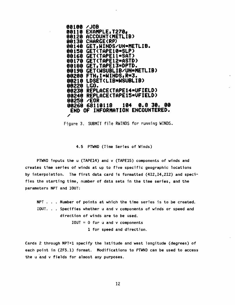
Figure 3 shows a sample SUBMIT file for running WINDS on the CDC 6600.

TAPE10 has the grid-point pressure fields in standard format. while TAPE11.

TAPE12 and TAPE13 have the surface air temperature. air-sea temperature

difference, and dew point depression grid fields. TAPE14 and TAPE15 are the

output u and v fields. WSLIBLIB contains the library of all subsequently

called sUbroutines. The input data card is in (4I2,I4,I2,2F5.1,I2) format.

The parameters are:

IYSTRT.

IMSTRT.

IDSTRT.

IHSTRT. .

KSETS

MODEL

The year (e.g.• 68) of the starting time

. The month (e.g., 11)

The date

The hour

The number sets to be analyzed

The model to be used to compute the surface winds.

Values 1-5 are reserved for temperature-independent

models. At present MODEL =1 for geostrophic winds

2 for surface winds by the balance equation

(Mahrt. 1975)

10

CNST2

CNST1

3 for gradient winds

4 empirical constants

6 use of Brown's model

8 use of Cardone's model.

If MODEL = 4 is specified, CNST1 is the fraction of the

gradient wind speed used as the surface wind speed and

CNST2 specifies the inflow turning angle in degrees to

the left of the geostrophic wind direction:

For MODEL = 6 or greater, CNST1 specifies the anemometer

height (em) assumed for the calculations. CNST2 specifies

the default relative humidity (decimal fraction).

If MODEL = 6 and CNST2<O, dew-point depression will read

from TAPE13.

ICNST = 0 wind components as output on TAPE14 and 15

= 1 wind stress components as output

= 2 total heat flux and latent heat flux

= 3 total heat flux and sensible Heat flux.

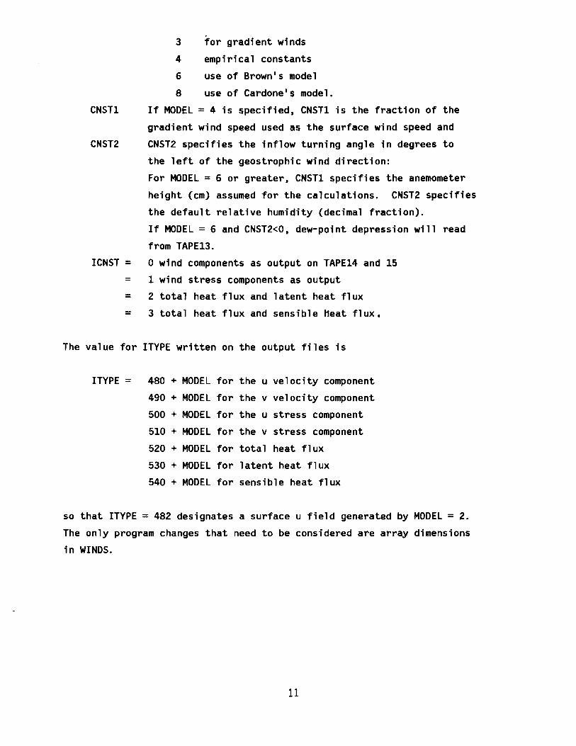
The value for ITYPE written on the output files is

ITYPE = 480 + MODEL for the u velocity component

490 + MODEL for the v veloeity component

500 + MODEL for the u stress component

510 + MODEL for the v stress component

520 + MODEL for total heat flux

530 + MODEL for latent heat flux

540 + MODEL for sensible heat flux

so that ITYPE = 482 designates a surface u field generated by MODEL = 2.

The only program changes that need to be considered are array dimensions

in WINDS.

11

88188 /JOB88118 EXA"PLE,T278.88128 ACCOUHT("ETLIB)88138 CHARGE (RP)88148 GET,WIHDS/UH-"ETLIB.88158 GET(TAPEI8-SLP)88168 GET(TAPE11-SAT)88178 GET(TAPEI2-ASTD)88188 GET,TAPEI3-DPTD.88198 GET(WSUBLIB/UH-"ETLIB)88288 FTN,I-WINDS,R-3.88218 LDSET(LIB-WSUBLIB)88228 LGO.88238 REPLACE(TAPE14-UFIELD)88248 REPLACE(TAPE15-UFIELD)88258 /EOR88268 68118118 184 8.8 38. 88

END OF INFOR"ATION ENCOUNTERED./

Figure 3. SUBMIT file RWINDS for running WINDS.

4.5 PTWND (Time Series of Winds)

PTWND inputs the u (TAPE14) and v (TAPE15) components of winds and

creates time series of winds at up to five specific geographic locations

by interpolation. The first data card is formatted (412.14.212) and speci­

fies the starting time. number of data sets in the time series. and the

parameters NPT and lOUT:

NPT . Number of points at which the time series is to be created.

lOUT. Specifies whether u and v components of winds or speed and

direction of winds are to be used.

lOUT = 0 for u and v components

1 for speed and direction.

Cards 2 through NPT+l specify the latitude and west longitude (degrees) of

each point in (2F5.1) format. Modifications to PTWND can be used to access

the u and v fields for almost any purposes.

12

4.6 PLOTGRD (Plotting)

PLOTGRD is the main program for performing graphical analysis on the

data sets generated by the METLIB wind analysis routines. Both scalar

and vector fields can be processed in a number of ways. and contour plots

and vector fields can be drawn on a continental outline background.

The primary purpose of PLOTGRD is for the user to set up arrays with

the proper dimensions. All subroutines use variable-dimensioned arrays and

need not be changed when data sets are changed.

The secondary purpose of PLOTGRD is to set default values for a number

of parameters which control the plotting. These values can be changed as

desired by the user.

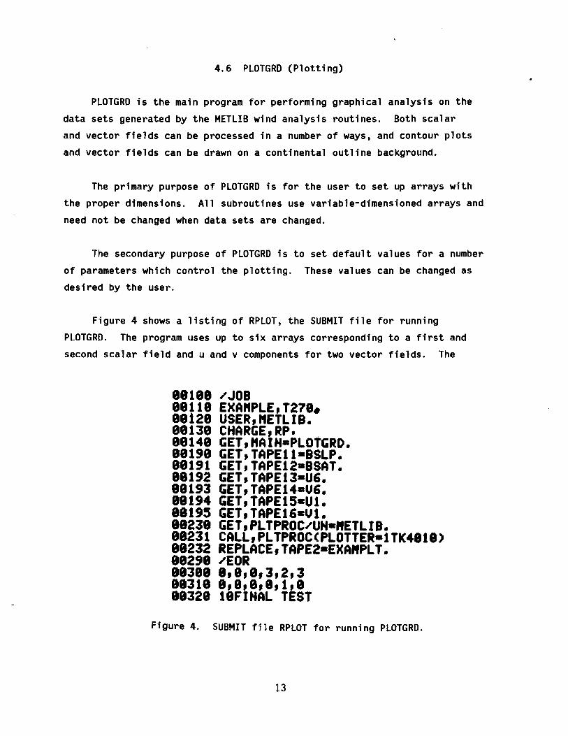
Figure 4 shows a listing of RPLOT. the SUBMIT file for running

PLOTGRD. The program uses up to six arrays corresponding to a first and

second scalar field and u and v components for two vector fields. The

88188 /JOB88118 EXA"PLE,T278.88128 USER,"ETLIB.88138 CHARGE,RP.18148 GET,HAIH-PLotGRD.88198 GET,TAPEI1-BSLP.88191 GET,TAPEI2-BSAT.88192 GET,TAPEI3-U6.88193 GET,TAPE14-U6.88194 GET,TAPE1S-UI.88195 GET,TAPEI6-Ul.88238 GET,PLTPROC/UH-"ETLIB.88231 CALL,PLTPROC(PLOTTER-ITK4818)88232 REPLACE,TAPE2-EXA"PLT.88298 /EOR88388 8,8,8,3,2,388318 8,8,8,1,1,888328 18FIHAL TEST

Figure 4. SUBMIT file RPLOT for running PLOTGRD.

13

logical unit numbers are assigned as TAPEll through TAPE16. These files

only need be attached if they are to be used. For example for plotting

vectors only. TAPEll and TAPE12 may be omitted.

The IIpLOTTER=1I parameter specifies the device which will perform the

plotting:

PLOTTER = ITK4818 specifies a Textronics 4818 terminal

PLOTTER = lCCWIDE specifies a CALCOMP plotter with wide paper

PLOTTER = lCCNARO specifies a CALCOMP plotter with narrow paper.

The first data card specifies what plots are to be made. The second card

specifies the starting time and the number of plots to be made. Cards 1 and 2

are read as list-directed (free format) input. so data values need only be

separated by commas or blanks. Card 3 is optional and is used to specify an

additional title for the bottom of the plot.

Data Card 1:

Variable

151

152

1512

IVI

Value--o

1

2

o1

2

o

1

o

1

Comment

no scalar fields are to be processed. If

151=0. set 152=1512=0 also.

scalar field 1 (array 51) is to be contoured.

scalar field 1 is to be read in but is not

to be contoured (i. e., is to be used only for

differencing. see 1512).

no second scalar field is to be processed.

scalar field 2 is to be contoured.

scalar field 2 is to be read in but not

contoured.

the difference of the scalar fields 51-52

is not to be contoured.

the difference 51-52 is to be contoured.

no vector fields are to be processed. if

IVl=O. set IV2=IV12=0 also.

wind vectors (arrows) only are to be drawn

for vector field 1 (arrays Ul and VI).

14

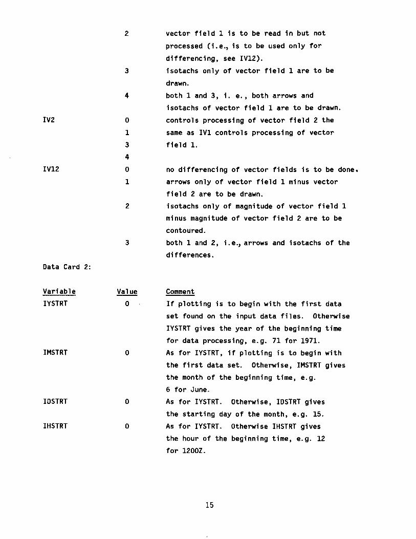
IV2

IV12

Data Card 2:

Variable

IYSTRT

IMSTRT

IDSTRT

IHSTRT

2

3

4

o1

3

4

o1

2

3

Value

o

o

o

o

vector field 1 is to be read in but not

processed (i.e., is to be used only for

differencing. see IV12).

isotachs only of vector field 1 are to be

drawn.

both 1 and 3. i. e .• both arrows and

isotachs of vector field 1 are to be drawn.

controls processing of vector field 2 the

same as IVI controls processing of vector

field 1.

no differencing of vector fields is to be done.

arrows only of vector field 1 minus vector

field 2 are to be drawn.

isotachs only of magnitude of vector field 1

minus magnitude of vector field 2 are to be

contoured.

both 1 and 2. i.e., arrows and isotachs of the

differences.

Comment

If plotting is to begin with the first data

set found on the input data files. Otherwise

IYSTRT gives the year of the beginning time

for data processing. e.g. 71 for 1971.

As for IYSTRT. if plotting is to begin with

the first data set. Otherwise. IMSTRT gives

the month of the beginning time. e.g.

6 for June.

As for IYSTRT. Otherwise. IDSTRT gives

the starting day of the month. e.g. 15.

As for IYSTRT. Otherwise IHSTRT gives

the hour of the beginning time. e.g. 12

for 1200Z.

15

KSETS

IBACK

o

o

N

If all data from the starting time until

the end of the input data files are to be

processed. If KSETS is greater than zero,

then KSETS of data will be processed,

beginning with the data set at time IYSTRT,

IMSTRT, IDSTRT, IHSTRT.

Note that setting IYSTRT=IMSTRT=IDSTRT=

IHSTRT=KSETS=O means that all data found on

the input files will be processed.

no background of continental outlines is to

be drawn.

Where N = 1,2, etc. a continental outline is

to be drawn every Nth map.

Data Card 3: This card provides any desired title at the bottom of the plot, given

the specification of 2 variables:

Variable Format Comment

NAUXTL 12 The number of characters in the

auxiliary title.

AUXTIT 7A10,A8 The character string which comprises the

title. Up to 78 characters are allowed.

If no auxiliary title is desired, either omit this data card entirely

or give NAUXTL the value O. An example of data card 3 is: 13EXAMPLE TITLE.

After running the example RPLOT of Figure 4 (via SUBMIT, RPLOT,

E=PMEL), one can view the generated plots on a Textronix terminal by typing

GET,EXAMPLT.

LNH. F=EXAMPLT.

If PLOTTER=1CCNARO is specified in RPLOT, then type

GET,EXAMPLT

16

PRESIN.

TEMPIN. .

ROUTE, EXAMPLT, DC=PR, UN=PMELTRM to send the plot to the CALCOMP plotter

PMEL.

Figures 5 and 6 are sample plots.

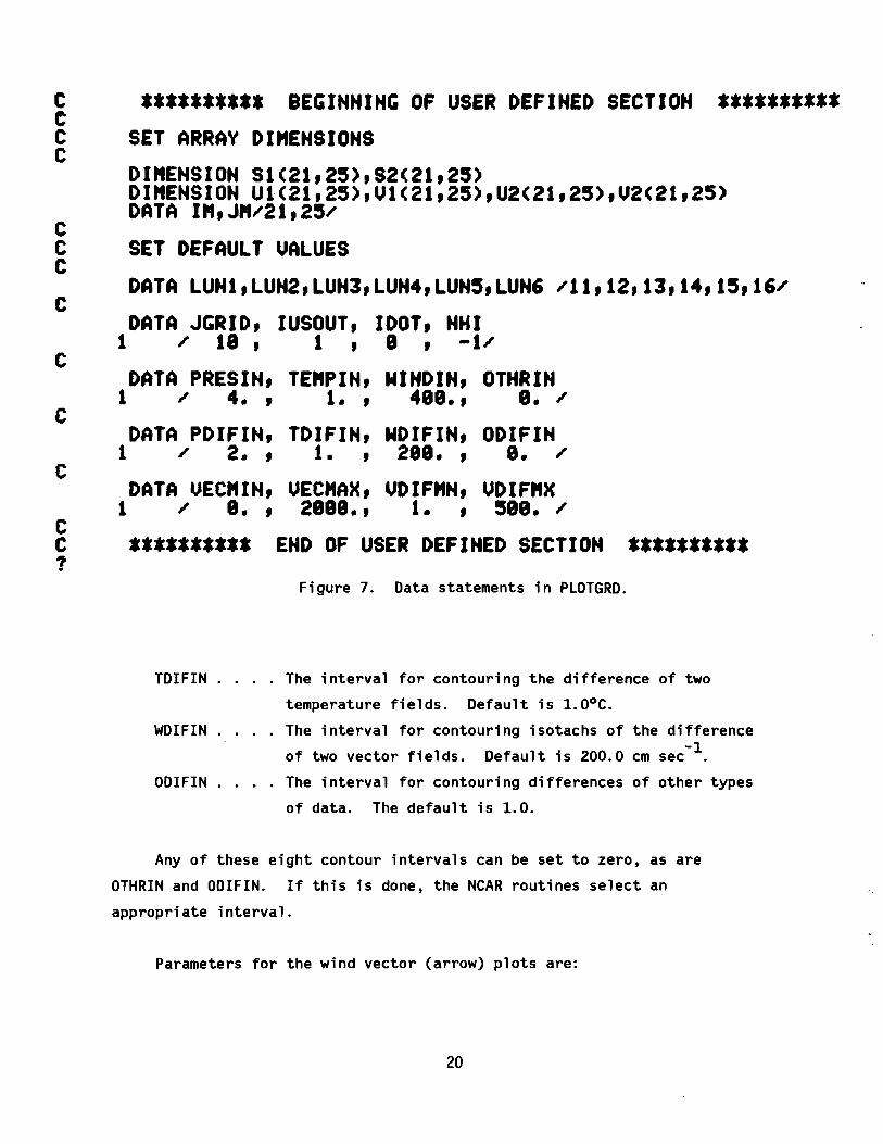
The next set of variables is assigned within PLOTGRD (Fig. 7) and can

be changed by editing a copied version of the program.

JGRIO .•.. The interval for drawing latitude and longitude lines.

Default is 10°.

IUSOUT.... Determines whether or not US state outlines are to be

drawn if continental outlines are drawn. Default of 1

gives state outlines. Set to 0 for no outlines.

lOOT..... 0 for continental outlines drawn by solid lines (default)

1 for continental outlines drawn by dotted lines

NHI ..... 0 if highs and lows are labelled by Hand L respectively

on all contour maps (pressure maps are always labelled

Hand L). -1 if highs and lows are not to be labelled

(default).

Contour intervals for various types of data are as follows:

. The contour interval for pressure fields. Default is 4.0 mb.

The contour interval for temperature fields. The default

is 1.00 C.

WINOIN. . . . The contour interval for isotachs of the wind fields.-1Default is 400.0 cm sec

OTHRIN . . . The contour interval for any other data type. The

default of 0.0 allows the NCAR routine to examine

the data and choose an appropriate interval.

Contour intervals for differences of data fields are as follows:

POIFIN.... The contour interval for contouring the differences of

two pressure fields. Default is 2.0 mb.

17

./ ~/

-

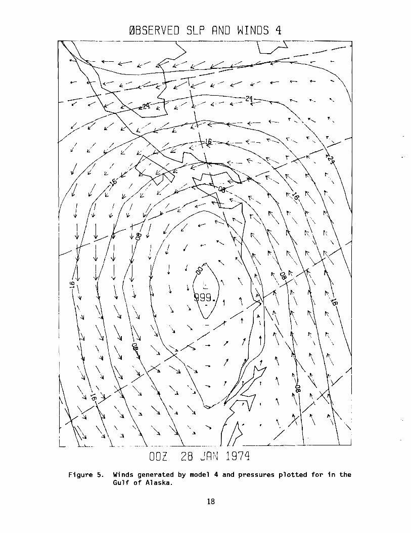
0BSERVED SLP RND WINDS 4-----------=>-------~-=-- -- ---<E-- ~ ___./" .___...-- ././- ..--

oc;- k· <- i:- .----

Figure 5. Winds generated by model 4 and pressures plotted for in theGulf of Alaska.

18

61

'o:>~xaHJ.OJ.ln~

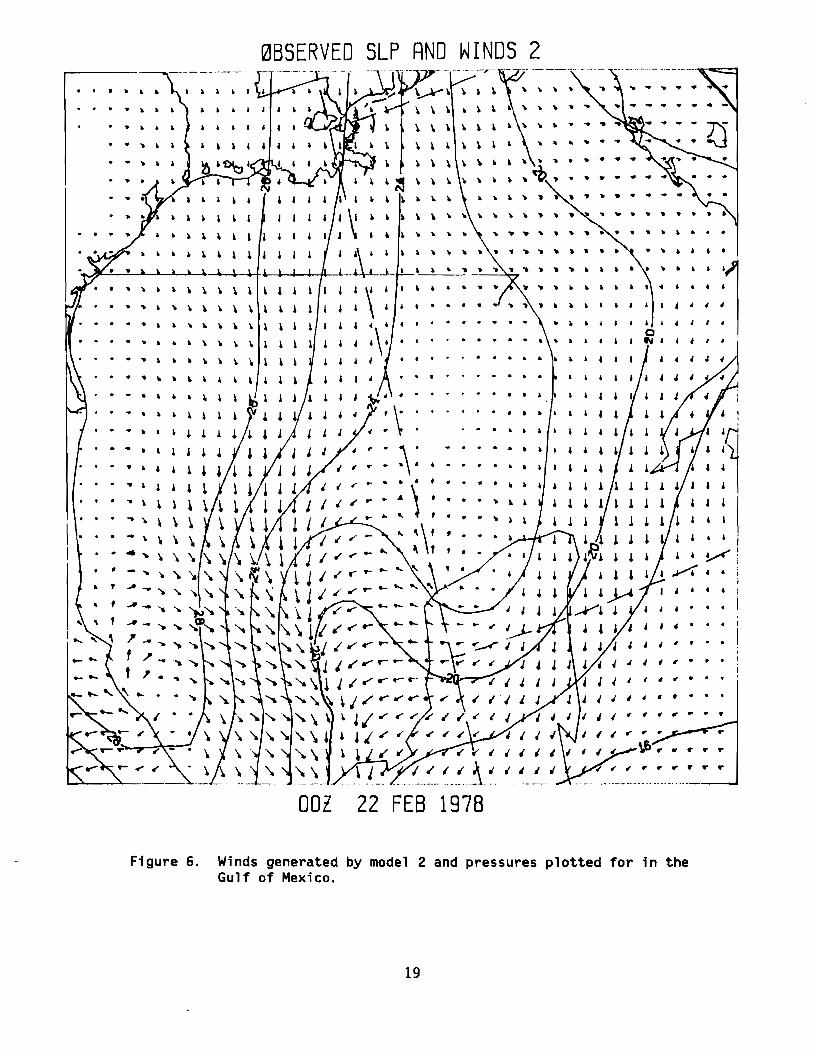
a4lu~~OJ.pallOldsa~nssa~dpueZlapowAqpale~auaBspu~M'9a~nB~~

9L61gjjZZtOO

..,...·...

1..••

.........,". ,...

".""... ,..'\..••....•'\••

,'\'\..,,,'\,'\..,,,,,,-~

,,,,,,T,

.~

,..,£

,......,,-.....

"."-,.,,-....• -4.....1'/1\f\\~"r-.",---",..._,

\\,....··\1

'\\\'\..·· ,,,'\..·· ,,t~\..· ~,,T·~

ff1,t,~

· tTrT1,TTf1,,. tT,,••. ,,,,,"

....'/'t

·....

·.'{, ••t\'

••ttt

t,t,

"'It~

••

,,",,'\'\

..

••

·... ·.

.....,.",

..,

....,..,.

...

,..

,....

,,...

"...."

....

......

.,..t,.,••

,,.....",.,...

,,,,..

'\'..,

•..,•,,,,,, ,,,'\

,,

,'1,•

tI

,,

••...-~II..,

.~,~

....

·~

·....,..

.,,,•••I,,,

.......JjJj...

·.., ·..",t•

•• I

i.Y1'

I"It

~,'r)tI

l""'~"t

",."""

""'(,.". ...,..,..ttt.,.,~..

'.t,.,.\I.,.....L.

ZSONIMON~dlSOjA~jSg0

DATA LUN1,LUN2,LUN3,LUN4,LUN5,LUN6 /11,12,13,14,15,16/

DATA JGRID, IUSOUT, lOOT, NHI1 / 18, 1, 8 , -1/

ccC

C

C ********** BEGINNING OF USER DEFINED SECTION **********eC SET ARRAV DIMENSIONSC

DIMENSION 91(21,23),S2(21,2S)DI"ENSION Ul(21,25),Ul(21,25),U2(21,2S),U2(21,25)DATA I",J"~21,25~

SET DEFAULT UALUES

c

c

C

cC?

DATA PRESIN, TE"PIN, MINDIN, OTHRIN1 / 4. , 1. , 488., 8. /

DATA PDIFIN, TOIFIN, MDIFIN, ODIFIN1 / 2. , 1. , 288. , 8. /

DATA VEC"IN, UECMAX, UOIFMH, UDIF"X1 / 8. , 2888. , I. , 588. /

********** END OF USER DEFINED SECTION **********Figure 7. Data statements in PLOTGRD.

TDIFIN .

WDIFIN .

ODIFIN .

The interval for contouring the difference of two

temperature fields. Default is 1.0o C.

The interval for contouring isotachs of the difference

of two vector fields. Default is 200.0 cm sec-1.

The interval for contouring differences of other types

of data. The default is 1.0.

Any of these eight contour intervals can be set to zero, as are

OTHRIN and ODIFIN. If this is done, the NCAR routines select an

appropriate interval.

Parameters for the wind vector (arrow) plots are:

20

VECMIN. .The smallest vector magnitude to be drawn. Default

is 0.0.

VECMAX. .The largest vector magnitude to be drawn. The plot

is scaled so that an arrow of this length will just

reach from one data point to the next. Default is-12000.0 cm sec. .

VDIFMN.....The smallest vector magnitude to be drawn when the

difference of two vector fields is being plotted. Any

vector smaller than this will not be plotted. Default-1is 1.0 cm sec. .

VDIFM .....The largest vector magnitude to be drawn when the

difference of two vector fields is being plotted.-1Default 1s 500.0 cm sec. .

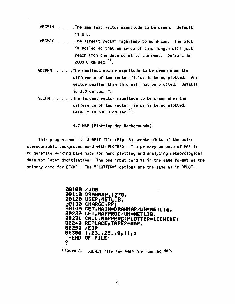
4.7 MAP (Plotting Map Backgrounds)

This program and its SUBMIT file (Fig. 8) create plots of the polar

stereographic background used with PLOTGRD. The primary purpose of MAP is

to generate working base maps for hand plotting and analyzing meteorological

data for later digitization. The one input card is in the same format as the

primary card for DECKS. The IIpLOTTER=1I options are the same as in RPLOT.

selll "'JOB89119 DRAWMAP,T271.99129 USER,METLIB.90130 CHARGE,RP)90149 GET,MAIH-DRAWMAP"'UH-"ETLIB.99230 GET,MAPPROC/UH-METLIB.99231 CALL,MAPPROC(PLOTTER-ICCWIDE)99249 REPLACE,TAPE2-MAP.99299 "'EORe9398 1,23.,25.,8,11,1

-END OF FILE-7

Figure 8. SUBMIT file for RMAP for running MAP.

21

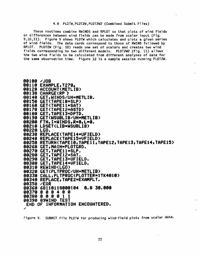
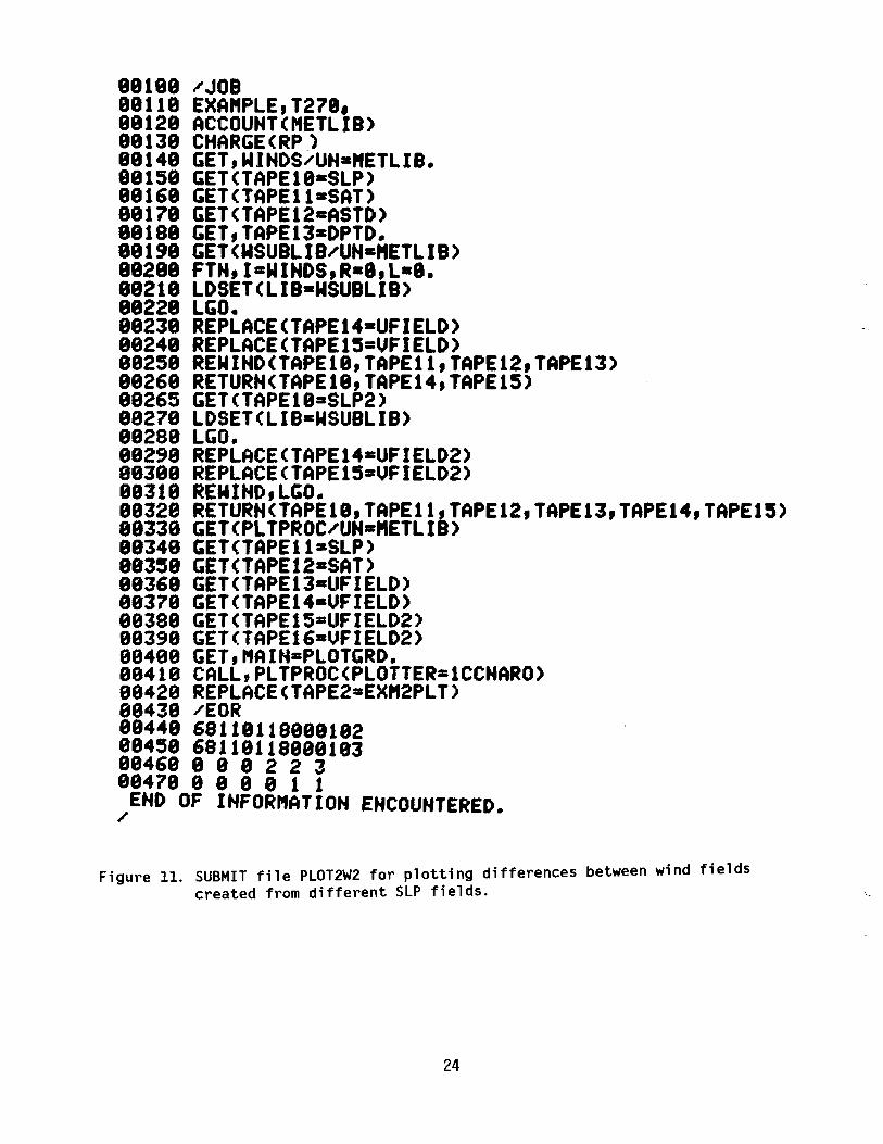
4.8 PLOTW,PLOT2W,PLOT2W2 (Combined Submit Files)

These routines combine RWINDS and RPLOT so that plots of wind fieldsor differences between wind fields can be made from scalar input (Fig.9,10,11). Figure 9 shows PLOTW which calculates and plots a given seriesof wind fields. The data cards correspond to those of RWIND followed byRPLOT. PLOT2W (Fig. 10) reads one set of scalars and creates two windfields corresponding to two different models. PLOT2W2 (Fig. 11) allowsthe two wind fields to be calculated from different analyses of data forthe same observation time. Figure 12 is a sample session running PLOT2W.

eel8a /JOBe8119 EXA"PLE,T279.99128 ACCOUNT(METLIB)98139 CHARGE (RP )99149 GET,WIHDS,UH=METLIB.99159 GET(TAPE19=SLP)89168 GET(TAPEll=SAT)99179 GET(TAPEI2=ASTD)88188 GET,TAPEI3=DPTD.89199 GET(WSUBLIB/UH="ETLIB)98298 FTN,I=WINDS,R=8,L-8.88218 LDSET(LIB-WSUBLIB)89229 LGO.99239 REPLACE(TAPEI4=UFIELD)99248 REPLACE(TAPEI5=UFIELD)99259 RETURN(TAPEI9,TAPE11,TAPEI2,TAPEI3,TAPEI4,TAPE1S)89269 GET,"AIN-PLOTGRD.99279 GET,TAPEll=SLP.99289 GET,TAPE12=SAT.99299 GET,TAPE13=UFIELD.99399 GET,TAPEI4=UFIELD.99319 REWIHD(LGO)89329 GET(PLTPROC/UH="ETLIB)99339 CALL,PLTPROC(PLOTTER=ITK4818)99349 REPLACE,TAPE2=EXA"PLT.e93S8 ,EOR99369 68119118898194 8.8 38.88899379 8 9 9 4 8 999388 9 9 9 9 1 199390 09WIHD TEST

END OF IHFOR"ATIOH ENCOUNTERED./

Figure 9. SUBMIT file PLOTW for producing wind-field plots from scalar data.

22

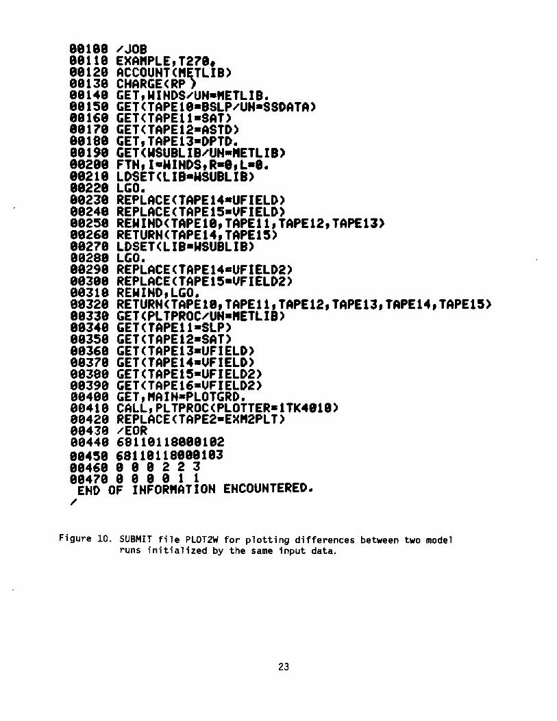
lIllI/JOB18118 EXA"PLE,T271,81128 ACCOUHT("ETLIB)88138 CHARGE(RP)88148 GET,WINDS/UN-"ETLIB.88158 GET(TAPEI8-SSLP/UN-SSOATA)88168 CET(TAPEI1-SAT>88178 GET(TAPEI2-ASTD)88188 CET,TAPEI3-DPTD.88191 CET(WSUBLIB/UH-"ETLIB)81288 FTH,I-WIHDS,R-8,L-8.88218 LDSET(LIB-WSUBLIB)88228 LCO.88238 REPLACE(TAPEI4-UFIELD)88248 REPLACE(TAPE1S-VFIELD)88258 REWIHD(TAPEI8,TAPEll,TAPEI2,TAPE13)88268 RETURH(TAPE14,TAPE1S)88278 LDSET(LIB-WSUBLIB)89288 LGO.88298 REPLACE(TAPEI4-UFIELD2)89388 REPLACE(TAPE1S-UFIELD2)89319 REWIND,LCO.88328 RETURH(TAPE11,TAPE11,TAPE12,TAPE13,TAPE14,TAPE1S)88338 GET(PLTPROC/UN-"ETLIB)88348 GET(TAPE11-SLP)88358 GET(TAPE12-SAT)89368 GET(TAPEI3-UFIELO)88378 CET(TAPEI4-UFIELO)88388 GET(TAPE1S-UFIELD2)88398 GET(TAPEI6-UFIELD2)B8480 GET,"AIN-PLOTGRD.09418 CAlL,PLTPROC(PLOTTER-ITK4118)88428 REPLACE(TAPE2-EX"2PLT)88438 /EOR80448 68118118818182ee4S8 681181188e8183e9468 8 8 e 2 2 3e9478 8 9 8 9 1 1

END OF INFOR"ATION ENCOUNTERED./

Figure 10. SUBMIT file PlOT2W for plotting differences between two modelruns initialized by the same input data.

23

99199 /JOB99118 EXA"PLE,T27e.98129 ACCOUNT(METLIB)98139 CHARGE(RP)88149 GET,WIHDS/UNa"ETLIB.98159 GET(TAPE19=SLP)89168 GET(TAPE11-SAT)98178 GET(TAPEI2-ASTD)89188 GET,TAPE13-DPTD.88198 GET(WSUBLIB/UNc"ETLIB)89288 FTN,I-WINDS,R-',L-••89218 LDSET(LIB-WSUBLIB)88228 LGO.88238 REPLACE(TAPEI4-UFIELD)99248 REPLACE(TAPE1S=UFIELD)99259 REWIND(TAPE19,TAPEll,TAPE12,TAPEI3)99269 RETURN(TAPE18,TAPE14,TAPE15)99265 GET(TAPE19=SLP2)98279 LOSET<LIBcWSUBLIB)99289 LGD.89298 REPLACE(TAPE14cUFIELD2)88388 REPLACE<TAPE15=UFIELD2)99318 REWIND,LCO.99328 RETURN(TAPEI8,TAPE11,TAPE12,TAPE13,TAPE14,TAPE1S)88339 GET(PLTPROC/UH="ETLIB)98349 CET(TAPE11-SLP)88358 GET(TAPE12-SAT)98369 GET<TAPE13-UFIELO)88379 GET(TAPE14-UFIELD)99389 GET(TAPE15=UFIELD2)99398 GET(TAPE16=VFIELD2)88409 GET,"AIH-PLOTGRD.99410 CALL,PLTPROC(PLOTTER=lCCNARO)99429 REPLACE<TAPE2-EX"2PLT)99439 /EOR99449 6811911889918289459 6811811888818388468 9 8 8 2 2 J88479 8 8 8 8 1 1

END OF INFOR"ATIOH ENCOUNTERED./

Figure 11. SUBMIT file PLOT2W2 for plotting differences between wind fieldscreated from different SLP fields.

24

~ALL·RATE·,1288,e,2CALL-TER"IN-8e/B7~14. 12.19.23.

N 0 A A / E R L "leA 88~e7/13.FA.. IlY:USER HU"BER: "ETlIBPASSWORD••••••••TER"INAL: 111, TTYRECOUER/ CHARGE: CHARGE,RP, ••••I •••tCHARGE,RP,8C697168.~GET,PlOT2W

/USER,P"ELTR"USER,PI1ELTR"./CHARGE,RP, ••••,I.IACSR, 2. 887UHTS./SUB"IT,PLOT2W

12. 18. 52.AETACCV/USER,ttETlIBUSER, "ETlIB./CHARGE,RP, ••••,I••ACSR, 2.8S8UHTS./ENQUIRE,JH-CCU

AGZYCCU HOT FOUHD./GET,EXA"PLT/lHH, FcEXA"PLT

Figure 12. Sample session with PLOT2W.

25

5. SUBROUTINE DOCUMENTATION

5.1 Introduction

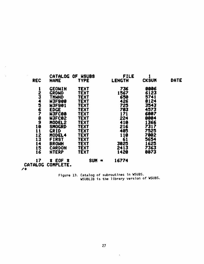
A catalog of sUbroutines on WSUBLIB is in Figure 13. Consult source

listings on WSUBS for calling sequences.

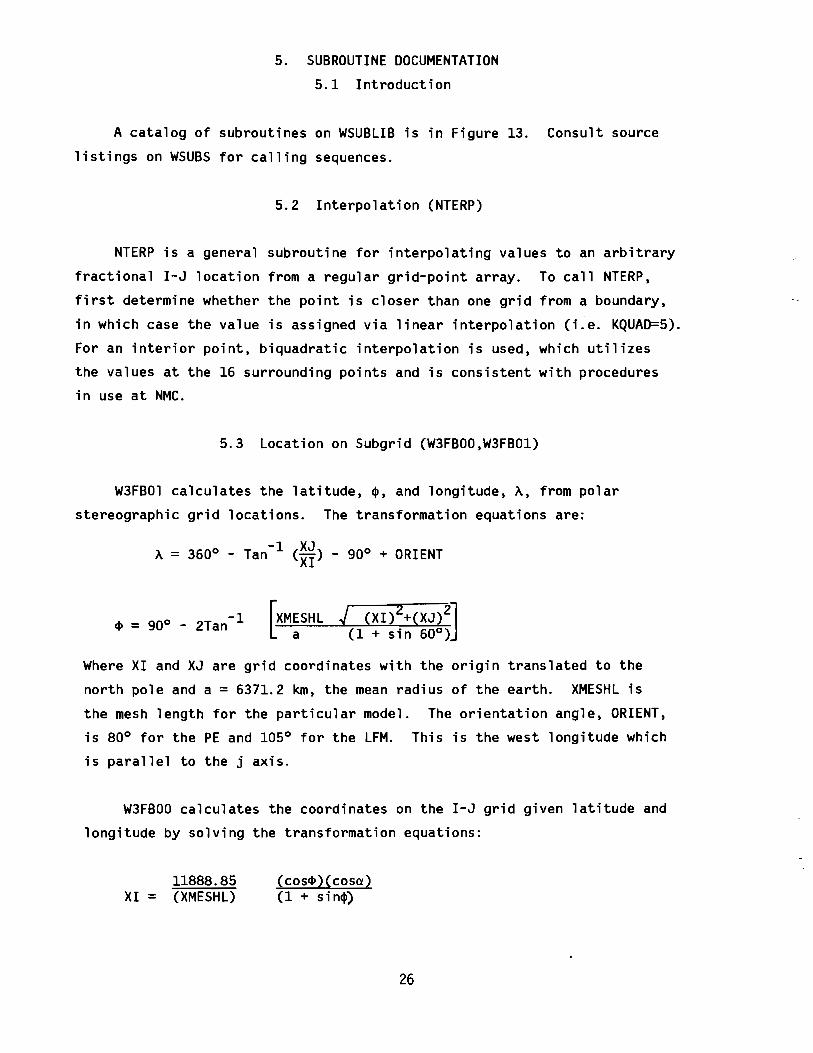
5.2 Interpolation (NTERP)

NTERP is a general subroutine for interpolating values to an arbitrary

fractional I-J location from a regular grid-point array. To call NTERP,

first determine whether the point is closer than one grid from a boundary,

in which case the value is assigned via linear interpolation (i.e. KQUAD=5).

For an interior point, biquadratic interpolation is used, which utilizes

the values at the 16 surrounding points and is consistent with procedures

in use at NMC.

5.3 Location on SUbgrid (W3FBOO,W3FB01)

W3FBOl calculates the latitude, ~, and longitude, A, from polar

stereographic grid locations. The transformation equations are:

-1 XJA = 360° - Tan (--) - 90° + ORIENTXI

-1~ = 90°- 2Tan rXMESHL j (XI)Z+(XJ)2]

l a (1 + sin 60°)

Where XI and XJ are grid coordinates with the origin translated to the

north pole and a = 6371.2 km, the mean radius of the earth. XMESHL is

the mesh length for the particular model. The orientation angle, ORIENT,

is 80° for the PE and 105° for the LFM. This is the west longitude which

is parallel to the j axis.

W3FBOO calculates the coordinates on the I-J grid given latitude and

longitude by solving the transformation equations:

11888.85XI = (XMESHL)

(cos~)(cosa)

(1 + sin~)

26

CATALOG OF WSUBS FILE 1REC HA"E TVPE LEHGTH CKSU" DATE

1 GEOWIH TEXT 736 888'2 GROWD TEXT IS67 61233 T"WND TEXT 6S8 57414 W3FB88 TEXT 426 81245 W3FB81 TEXT 72S 3S436 EDGE TEXT 783 4S737 N3FC88 TEXT 171 61178 W3FCI2 TEXT 224 11149 "ODEL2 TEXT 411 136'

II S"OGRD TEXT 216 731711 GRID TEXT 415 752512 "ODEL4 TEXT 118 718213 FIRST TEXT 61 565414 BROWH TEXT 3825 162515 CARDON· TEXT 2413 736316 NTERP TEXT 1428 8873

17 * EOF * SU" • 16774CATALOG CO"PLETE.

/+Figure 13. Catalog of subroutines in WSUBS.

WSUBLIB is the library version of WSUBS.

27

XJ = (11888.85)\

XMESHL J((COS4l) (sina)\\ 1 + sin41 ) ,

where a =3600- (A + 900 - ORIENT). The pole location is then subtracted

to locate the point on the standard grids.

5.4 Speed and Direction (W3FC02,W3FCOO)

W3FC02 computes the speed and direction in the meteorological

convention of the wind from grid-oriented vector components. The

speed is simply SQRT(u2 + v2 ). The wind direction is found from

D = TAN- 1 XJ - TAN- 1 YXI U

where XI and XJ are defined as in W3FBOO. W3FCOO performs the reverse

operation.

5.5 Thermal Wind (TMWND)

This subroutine calculates the non-dimensional thermal u and v wind

component fields. These calculations are made only if one of models 6-10

is to be used. The vertical gradient of the geostrophic wind in the boundary

layer is assumed to depend only on the surface horizontal temperature gradient

computed by central differences and the Coriolis parameter:

aTax

where g is the gravitational acceleration; f, the Coriolis parameter; and

air temperature (SAT) is taken for the boundary layer average temperature, T,

at each grid point.

5.6 GRIDSET (GRIDSET)

GRIDSET reads in IGRID, IFACT, and other parameters and adjusts them

according to the degree of interpolation and the grid system used.

28

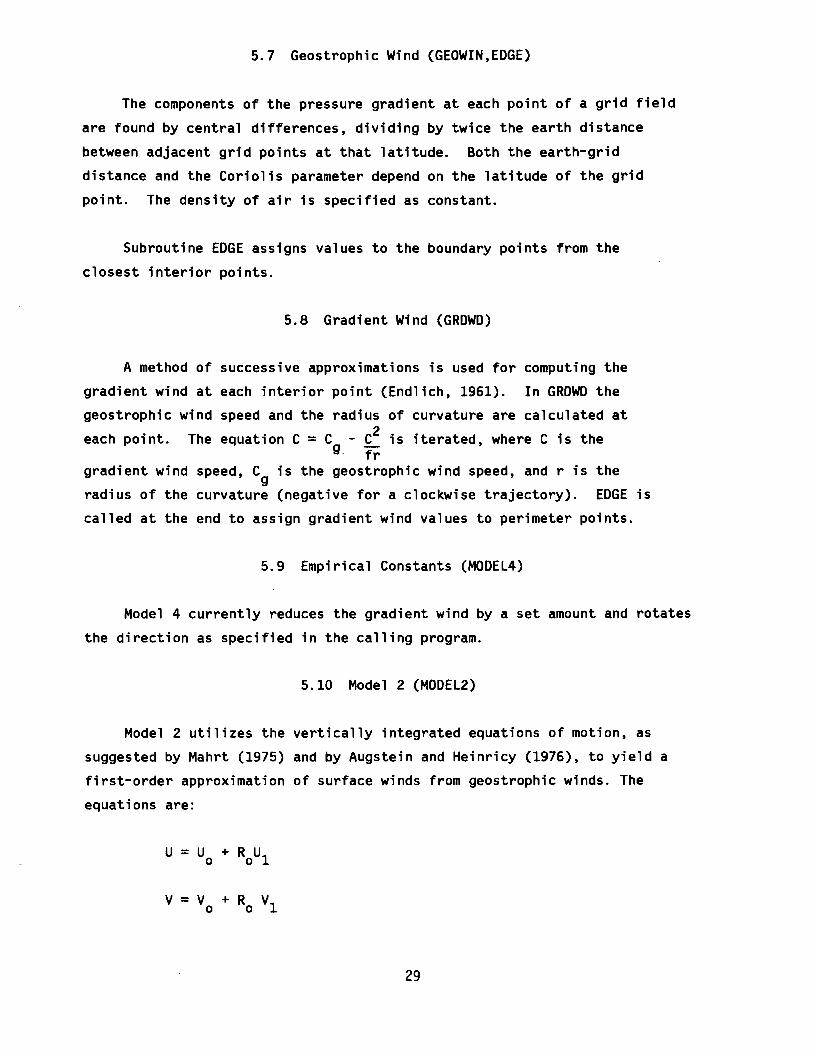
5.7 Geostrophic Wind (GEOWIN,EOGE)

The components of the pressure gradient at each point of a grid field

are found by central differences, dividing by twice the earth distance

between adjacent grid points at that latitude. Both the earth-grid

distance and the Coriolis parameter depend on the latitude of the grid

point. The density of air is specified as constant.

Subroutine EDGE assigns values to the boundary points from the

closest interior points.

5.8 Gradient Wind (GROWO)

A method of successive approximations is used for computing the

gradient wind at each interior point (Endlich, 1961). In GROWO the

geostrophic wind speed and the radius of curvature are calculated at

each point. The equation C = C - C2 is iterated, where C is theg fr

gradient wind speed, C is the geostrophic wind speed, and r is theg

radius of the curvature (negative for a clockwise trajectory). EDGE is

called at the end to assign gradient wind values to perimeter points.

5.9 Empirical Constants (MOOEL4)

Model 4 currently reduces the gradient wind by a set amount and rotates

the direction as specified in the calling program.

5.10 Model 2 (MODEL2)

Model 2 utilizes the vertically integrated equations of motion, as

suggested by Mahrt (1975) and by Augstein and Heinricy (1976), to yield a

first-order approximation of surface winds from geostrophic winds. The

equations are:

U = U + R U1o 0

v = V + R VIo 0

29

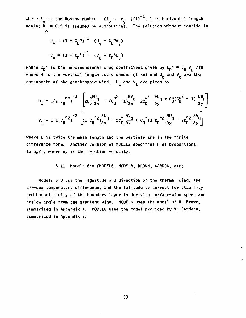
where R is the Rossby number (R = V (fl)-l; 1 is horizontal length0 0 g

scale; R = 0.2 is assumed by subroutine). The solution without inertia is0

U = (1+ C *)-1 (u - C *V )0 0 g o g

V = (1 + C *)-1o 0

where CO* is the nondimensional drag coefficient given by CO* = Co Vg /fH

'where H is the vertical length scale chosen (1 km) and U and V are theg gcomponents of the geostrophic wind. U1 and VI are given by

av *2 au + C*(C*2 _ 1) au ~-1)--9 -2C --9 0 0 --9

ax 0 ay ay

* av * *2 au *2 av ~2CO~ + CD (I-CD )~ - 2CO ~J

where L is twice the mesh length and the partials are in the finite

difference form. Another version of MOOEL2 specifies H as proportional

to u*/f, where u* is the friction velocity.

5.11 Models 6-8 (MOOEL6, MOOEL8, BROWN, CARDON, etc)

Models 6-8 use the magnitude and direction of the thermal wind, the

air-sea temperature difference, and the latitude to correct for stability

and baroclinicity of the boundary layer in deriving surface-wind speed and

inflow angle from the gradient wind. MOOEL6 uses the model of R. Brown,

summarized in Appendix A. MOOEL8 uses the model provided by V. Cardone,

summarized in Appendix B.

30

6. ACKNOWLEDGEMENTS

This report is a contribution to the Marine Services Project at Pacific

Marine Environmental laboratory. Subroutines W3FBOO and W3FBOI and subroutine

NTERP are adaptations of subroutines in use at the National Meteorological,

Center. Our thanks to Clifford M. Fridlind, Matthew H. Hitchman, Steven

Ghan and Jon O. Nestor who have contributed to the development of METlIB.

T. liu contributed substantially to Appendix A. V. Cardone provided a copy

of the computer program of his boundary layer model. R. Brown was supported

in part by the Jet Propulsion laboratory during preparation of this memorandum.

31

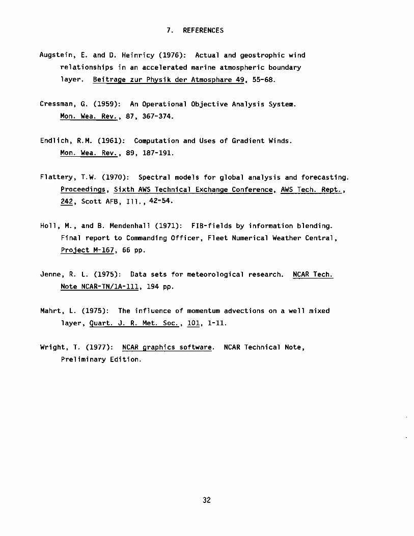
7. REFERENCES

Augstein. E. and D. Heinricy (1976):

relationships in an accelerated

layer. Beitrage zur Physik der

Actual and geostrophic wind

marine atmospheric boundary

Atmosphare 49. 55-68.

Cressman. G. (1959): An Operational Objective Analysis System.

Mon. Wea. Rev .• 87. 367-374.

Endlich. R.M. (1961): Computation and Uses of Gradient Winds.

Mon. Wea. Rev .• 89. 187-191.

Flattery. T.W. (1970): Spectral models for global analysis and forecasting.

Proceedings. Sixth AWS Technical Exchange Conference. AWS Tech. Rept .•

242. Scott AFB. 111 .• 42-54.

Holl. M.• and B. Mendenhall (1971): FIB-fields by information blending.

Final report to Commanding Officer. Fleet Numerical Weather Central.

Project M-167. 66 pp.

Jenne. R. L. (1975): Data sets for meteorological research. NCAR Tech.

Note NCAR-TN/1A-111. 194 pp.

Mahrt. L. (1975): The influence of momentum advections on a well mixed

layer. Quart. J. R. Met. Soc .• 101. 1-11.

Wright. T. (1977): NCAR graphics software. NCAR Technical Note.

Preliminary Edition.

32

Appendix A: DERIVATION OF THE UNIVERSITY OF WASHINGTON (BROWN)

PLANETARY BOUNDARY LAYER MODEL

1. SOLUTION FOR THE PBL WITH NEUTRAL STABILITY

An appropriate set of non-dimensionalized equations for a non-acceler­

ating lower atmosphere is

V + E2

(KU) - P /pz z x = o (1)

U - E2

(KV) + P /pz z y = o (2)

where E is an Ekman number defined by E = 6/H, with 62 = 2K/f; H is an

arbitrary scale height; f is the Coriolis parameter; K is an eddy coeffic-

u*, G, 6, z , p , T , and L. All other terms use000

A continuous solution for the domain 0 ~ z ~ ~ can bestandard notation.

ient, K is its mean; V is the characteristic velocity scale; z = z/H;A 0

V = V/V. Hats denote dimensional variables while characteristic valueso

are always dimensional:

obtained by considering three scale heights H and the appropriate solution

for each regime is given in Table 1.

Table 1: Flow Solutions for Scale Heights H above the Surface

H E Equations Solutions

~O y + '\/P/p = 0 Geostrophic (w/corrections)

0[6J o[1] (1&2) with E= 1 Ekman/Taylor layer (3)

K constant U e-t[cos(a-t) !k cos tJ= = cos a -G G

V GV

sin a + e-t[sin(a-t) !k sin tJ- = -0 G G

U ~G at t ~ ~

U ~ U at t ~ 0-0

Cont.

33

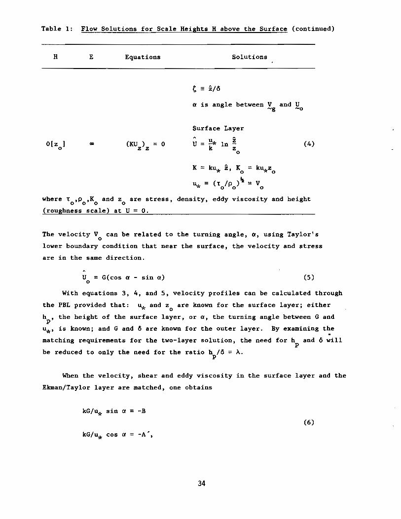
Table 1: Flow Solutions for Scale Heights H above the Surface (continued)

H

O[z ]o

E Equations

(KU) = 0z z

Solutions

a is angle between V and U....g ....0

Surface Layer

A ZU =~* In

k zo

K = ku* z, Ko =ku*zo

u - (t /p )~ =V* - 000

(4)

where t ,P ,K and z are stress, density, eddy viscosity and height000 0

(roughness scale) at U = O.

The velocity V can be related to the turning angle, a, using Taylor'so

lower boundary condition that near the surface, the velocity and stress

are in the same direction.

U = G(cos a - sin a)o

(5)

With equations 3, 4, and 5, velocity profiles can be calculated through

the PBL provided that: u* and zo are known for the surface layer; either

h , the height of the surface layer, or a, the turning angle between G andp

u*, is known; and G and 6 are known for the outer layer. By examining the

matching requirements for the two-layer solution, the need for hand 6 willp

be reduced to only the need for the ratio h /6 = A.p

When the velocity, shear and eddy viscosity in the surface layer and the

Ekman/Taylor layer are matched, one obtains

kG/u* sin a = -B

(6)

kG/u* cos a = -A',

34

where A~ and B are similarity parameters which depend on the single

similarity parameter, A. So,

AB = e /(2ACOSA)

A~ = -In AE - (cos A - sin A)/(2A cos A)s

(7)

(8)

The solution is completed by adding an empirical relation for z aso

a function of u* and assigning values to the similarity parameter, A.

There exist several choices for zo(u*). We have examined several

possibilities and have chosen the empirical relation from Kondo (1975)

(see Section IX) for use in the model. An iterative solution for u* is

needed.

2. THE NEUTRAL PBL WITH SECONDARY FLOW IN THE EKMAN/TAYLOR LAYER

It has been shown that the first-order closure (K-theory) solution

for the Ekman/Taylor layer is unstable to infinitesimal perturbations

and therefore doesn't exist (see, e.g., Brown, 1974). There is a non­

linear equilibrium finite perturbation solution (Brown, 1970) and this

correction has been incorporated in the model. The basic mean flow is

altered such that (U,V,W) = (UE'VE) + (U2

'V2

) + (u2 ,v2

,w2

) where (UE'VE)

is the solution of the homogeneous equation (3), (U2

'V2

) are the mean flow

modifications, and (u2

,v2

,w2

) are the zero mean secondary flow. The finite

perturbation modifies the basic Ekman/Taylor equation (3) with a forcing

function depending on w2v

2on the right-hand side of the second equation.

zThe amended equations for u* is

kG(sina+l3) = -B

u*

35

(9)

(10)

kG(cosa+)') -A ~ (11)=

u*

Awhere f3

-e U2

(A)= 2 cos At

cos A - sin A U2

+ U2)' = 2 cos A

t

evaluated at t = A.

The neutral value of U2 is given in Brown (1970).

3. THE MODIFIED EKMAN/TAYLOR LAYER WITH THERMAL WIND

When thermal wind is added to the model, the pressure gradient term in

(1) and (2) becomes a function of (T , T ), and, under the approximation thatx y

the temperature gradient is constant with height,

P /p = (P /p) 0 + (g/TO)TAZ.X X z= x

The equation for the geostrophic balance throughout the layer may be written

(U ,V ) = (U ,V ) + (uT,vT) tg g go go

(uT,vT) = ~ (-T ,T ), (U ,V ) = (cos a, sin a).o y x go go

The thermal wind must be added to (3) and the equations for f3 and)' become:

A ~ A + sin A

u2t] t=Af3-e cos v

T+=

{~:: : - ~inA

e

A+A] ~+ {2eA

1

cos A}VT)' = 2 cos A

+ U + cos A - sinAu}2 2 cos A 2t t=A

while (9) remains the fundamental equation for u*(G).

36

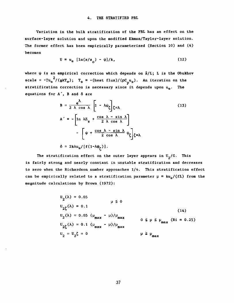
4. THE STRATIFIED PBL

Variation in the bulk stratification of the PBL has an effect on the

surface-layer solution and upon the modified Ekman/Taylor-layer solution.

The former effect has been empirically parameterized (Section 10) and (4)

becomes

(12)

T* = -(heat flux)/(pC u*). An iteration on thep

stratification correction is necessary since it depends upon u*. The

where ~ is an empirical correction which depends on z/L; L is the Obukhov2

scale = -Tu* /(gkT*);

equations for A I, B and (, are

A

~ - ~tJt=AB =e

2 A cos A

AI - [In ARscos A - sin

AJ= + 2 A cos A

[~ +cos A - sin A

~tJt=A- 2 cos A

(13)

The stratification effect on the outer layer appears in U2/G. This

is fairly strong and nearly constant in unstable stratification and decreases

to zero when the Richardson number approaches 1/4. This stratification effect

can be empirically related to a stratification parameter ~ = ku*/(fL) from the

magnitude calculations by Brown (1972):

U2t

(A) = 0.1

U2 (A) = 0.05 (~max - ~)/~max

U2t (A) = 0.1 (~max - ~)/~max

U2 = u2t = 0

(14)

o ~ II ~ II (Ri = 0.25)... "'max

37

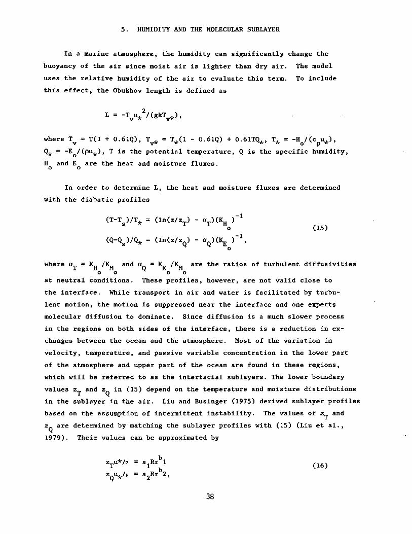
5 . HUMIDITY AND THE MOLECULAR SUBLAYER

In a marine atmosphere, the humidity can significantly change the

buoyancy of the air since moist air is lighter than dry air. The model

uses the relative humidity of the air to evaluate this term. To include

this effect, the Obukhov length is defined as

where Tv =T(l + O.61Q), Tv* =T*(l - O.61Q) + O.61TQ*, T* = -Ho/(cpu*),

~ = -Eo/(pu*), T is the potential temperature, Q is the specific humidity,

Hand E are the heat and moisture fluxes.o 0

In order to determine L, the heat and moisture fluxes are determined

with the diabatic profiles

(15)

where aT = ~ /~ ando 0

at neutral conditions.

aQ = ~ /~ areo 0

These profiles,

the ratios of turbulent diffusivities

however, are not valid close to

the interface. While transport in air and water is facilitated by turbu-

lent motion, the motion is suppressed near the interface and one expects

molecular diffusion to dominate. Since diffusion is a much slower process

in the regions on both sides of the interface, there is a reduction in ex­

changes between the ocean and the atmosphere. Most of the variation in

velocity, temperature, and passive variable concentration in the lower part

of the atmosphere and upper part of the ocean are found in these regions,

which will be referred to as the interfacial sublayers. The lower boundary

values zT and zQ in (15) depend on the temperature and moisture distributions

in the sublayer in the air. Liu and Businger (1975) derived sublayer profiles

based on the assumption of intermittent instability. The values of zT and

zQ are determined by matching the sublayer profiles with (15) (Liu et al.,

1979). Their values can be approximated by

(16)

38

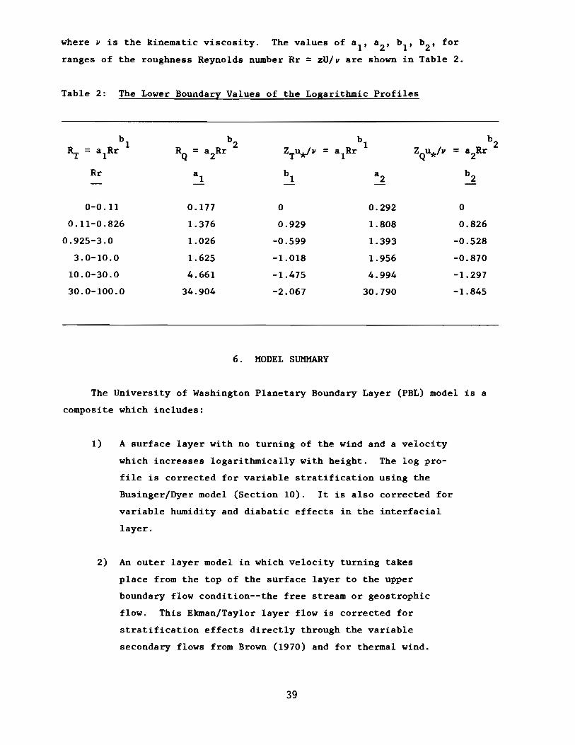
where v is the kinematic viscosity. The values of aI' a2

, b 1 , b2

, for

ranges of the roughness Reynolds number Rr =zU/v are shown in Table 2.

Table 2: The Lower Boundary Values of the Logarithmic Profiles

~

b1

b2

ZTu*/vb

1ZQu*/v

b2= a Rr R

Q = a2Rr = a

1Rr = a

2Rr

1

Rr a1

b1

a2

b2

0-0.11 0.177 0 0.292 0

0.11-0.826 1.376 0.929 1.808 0.826

0.925-3.0 1.026 -0.599 1.393 -0.528

3.0-10.0 1.625 -1.018 1.956 -0.870

10.0-30.0 4.661 -1. 475 4.994 -1. 297

30.0-100.0 34.904 -2.067 30.790 -1.845

6. MODEL SUMMARY

The University of Washington Planetary Boundary Layer (PBL) model is a

composite which includes:

1) A surface layer with no turning of the wind and a velocity

which increases logarithmically with height. The log pro­

file is corrected for variable stratification using the

Businger/Dyer model (Section 10). It is also corrected for

variable humidity and diabatic effects in the interfacial

layer.

2) An outer layer model in which velocity turning takes

place from the top of the surface layer to the upper

boundary flow condition--the free stream or geostrophic

flow. This Ekman/Taylor layer flow is corrected for

stratification effects directly through the variable

secondary flows from Brown (1970) and for thermal wind.

39

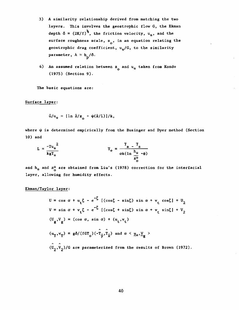
3) A similarity relationship derived from matching the two

layers. This involves the geostrophic flow G, the Ekman

depth 6 = (2K/f)~, the friction velocity, u*, and the

surface roughness scale, z , in an equation relating theo

geostrophic drag coefficient, u*/G, to the similarity

parameter, A =h /6.p

4) An assumed relation between zo and u* taken from Kondo

(1975) (Section 9).

The basic equations are:

Surface layer:

u/u* = [In z/zo - ~(z/L)l/k,

where ~ is determined empirically from the Businger and Dyer method (Section

10) and

2L = -Tu*---

kgT*

T Ta - s

hak(ln ..!:.. -~)

z*o

and h* and z~ are obtained from Liu's (1978) correction for the interfacial

layer, allowing for humidity effects.

Ekman/Taylor layer:

u = cos a + u t -t [(cost sint) sin a + v costl + U2et t

V = sin a + v t -t [(cost + sint) sin a + v sintl + V2et t

(U ,V ) = (cos a, sin a) + (ut'Vt )g g

(uT,vT) = g6/(fGT )(-TA,TA) and a < ~,V >o y x ~g

(U2 ,V2)/G are parameterized from the results of Brown (1972).

40

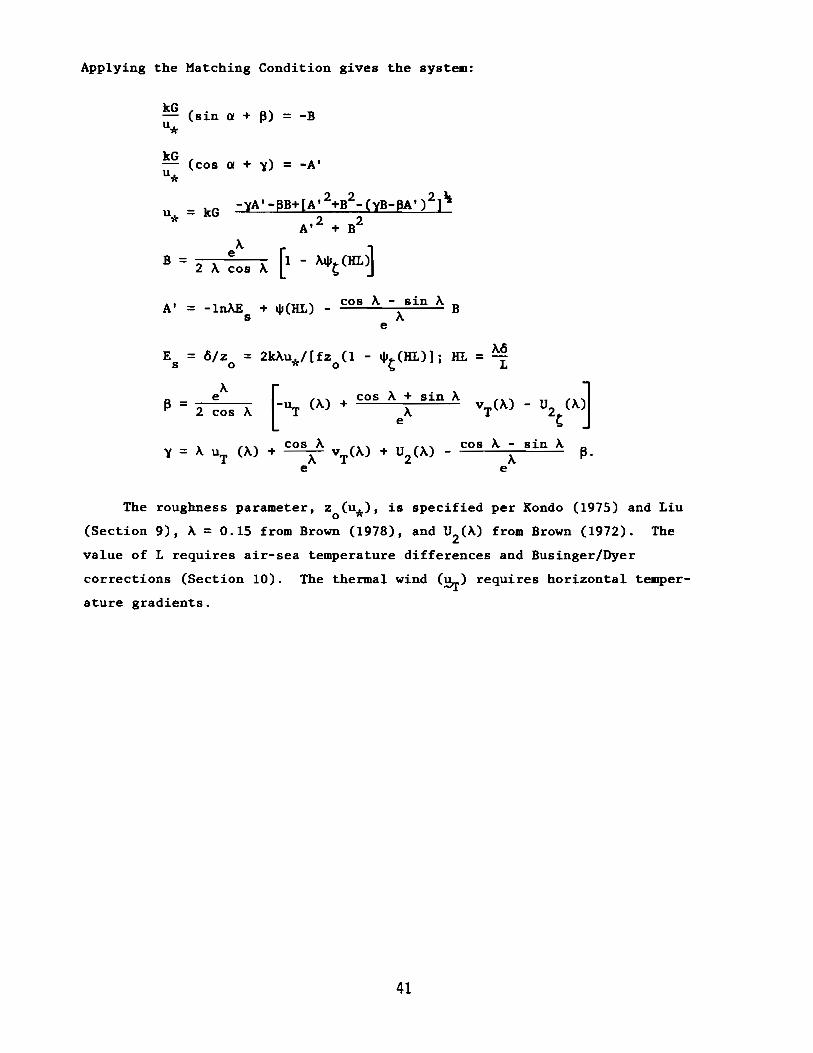
Applying the Matching Condition gives the system:

kG(sin ex + 13) = -B

u*

kG(cos ex + y) = -AI

u*

u* = kG-yA'-I3B+[A,2+B2_(YB-PA,)2]\

A,2 + B2

A

[1 - NPC(HL~B e= 2 A cos A

AI -IME + ..,(HL) cos A - sin A B= -s Ae

E 6/z 2kAu*/[ fz 0 (l - "'C(HL)]j HLA6= = =s 0 L

cos A -

Ae13 = -"--­

2 cos A [-u (A) + cos A + sin A

T Ae

+ COSAA vT(A) + U2

(A) ­e

Ae

The roughness parameter, zo(u*), is specified per Kondo (1975) and Liu

(Section 9), A =0.15 from Brown (1978), and U2 (A) from Brown (1972). The

value of L requires air-sea temperature differences and Businger/Dyer

corrections (Section 10). The thermal wind (Br) requires horizontal temper­

ature gradients.

41

7. PROGRAM FLOW DIAGRAM

G, f, TS (surface temp.), TZ, RH (temp. and relative humidity at height z),TX, TY (horizontal temp. gradient w.r.t. surface wind in deg/100 km), A

Subroutine UW4 containsthree nested do-loops. The outer­

most iterates on the stratification param­eter z/L according to a model suggested by Liu

(1978) to account for humidity and molecular sublayereffects. The middle one iterates on u* and a withsimilarity relations suggested by Brown (1978). The

innermost one iterates on a with a surfacediabatic profile from Busigger-Dyer (see

Brown, 1974) and an empirical relationfor z suggested by Kondo (1975).

o

USR (u*), ALPHA, zo' U (z meters), ZL (z/L),

H (heat flux), UT, VT (thermal wind components)o

8. MODEL SENSITIVITY

The model is based upon the ~ formulation of Businger-Dyer and the Kondo

(1975) zo(u*) relation. Other aspects which differ from previous models

are: the inclusion of equilibrium producing secondary flow in the outer

layer; adding a molecular sublayer and relative humidity effect; and adding

a thermal wind. The importance of each of these terms has been investi­

gated by varying the basic parameters and checking output variations for

representative cases.

42

Hf

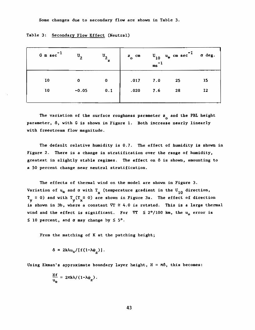
Some changes due to secondary flow are shown in Table 3.

Table 3: Secondary Flow Effect (Neutral)

G m-1

U2

U2

U10

-1Ci deg.sec z cm u* cm sec

0z-1

ms

10 0 0 .017 7.0 25 15

10 -0.05 0.1 .020 7.6 28 12

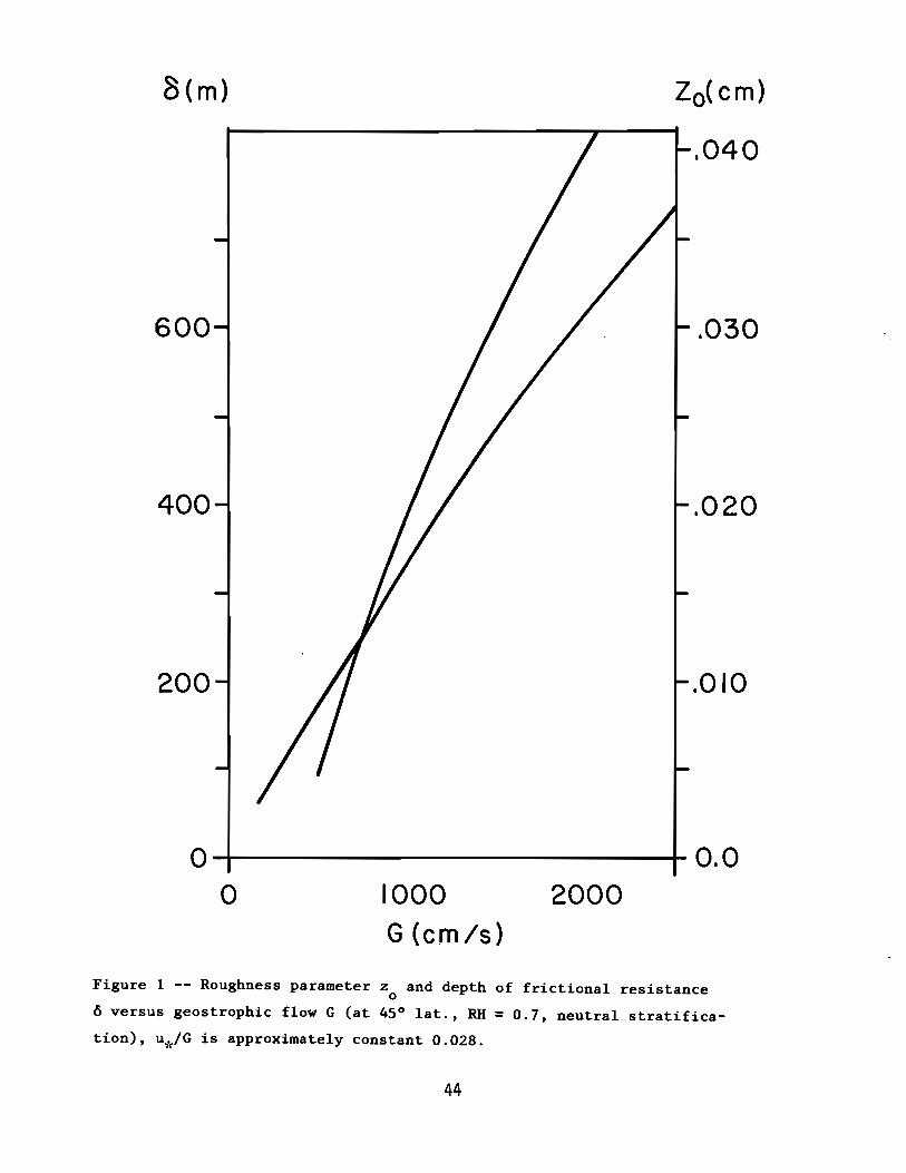
The variation of the surface roughness parameter z and the PBL heighto

parameter, 0, with G is shown in Figure 1. Both increase nearly linearly

with freestream flow magnitude.

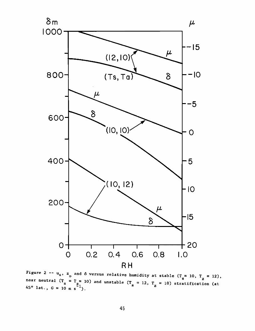
The default relative humidity is 0.7. The effect of humidity is shown in

Figure 2. There is a change in stratification over the range of humidity,

greatest in slightly stable regimes. The effect on ° is shown, amounting to

a 50 percent change near neutral stratification.

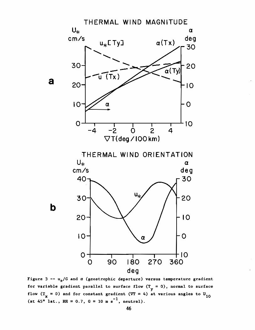
The effects of thermal wind on the model are shown in Figure 3.

Variation of u* and Ci with Tx

(temperature gradient in the U10

direction,

T =0) and with T (T =0) are shown in Figure 3a. The effect of directiony y x

is shown in 3b, where a constant VT ~ 4.0 is rotated. This is a large thermal

wind and the effect is significant. For VT ~ 2°/100 km, the u* error is

~ 10 percent, and Ci may change by ~ 5°.

From the matching of K at the patching height;

Using Ekman's approximate boundary layer height, H = no, this becomes:

= 2nkA/ (l-~ ).u* z

43

8(m)

600

400

200

.040

,030

.020

.010

0-1--------------;- 0.0o 1000

G(cm/s)

2000

Figure 1 -- Roughness parameter z and depth of frictional resistanceo

6 versus geostrophic flow G (at 45° lat., RH = 0.7, neutral stratifica-

tion), u*/G is approximately constant 0.028.

44

8mI000.....--~-----------,

800 -10

-5

o

5

10

15

o~-~----r--""""'--r---r- 20o 0,2 0.4 0.6 0.8 1.0

RHFigure 2 -- u*. z and 6 versus relative humidity at stable (T = 10. T = 12).

o s znear neutral (T = T = 10) and unstable (T = 12. T = 10) stratification (at

s ~1 s z45° lat., G = 10 m s ).

45

o10

THERMAL WIND MAGNITUDE

U* acm/s

u*[ TyJ a(Tx)deg30

..................

.........30 -........ 20

--~~--

a ""-u (Tx)20 10

o--- -----.------r-----.r----~ ..... 10-4 -2 0 2 4

\IT(deg /100 km)

THERMAL WI NO ORIENTATIONU* a

cm/s deg40 30

b30

20

10

20

10

o

o~- --r-----...,..----+ 10o 90 180 270 360

degFigure 3 -- u*/G and a (geostrophic departure) versus temperature gradient

for variable gradient parallel to surface flow (T = 0), normal to surfacey

flow (Tx =0) and for constant gra~~ent (VI =4) at various angles to UIO(at 45° lat., RH = 0.7, G = 10 m s ,neutral).

46

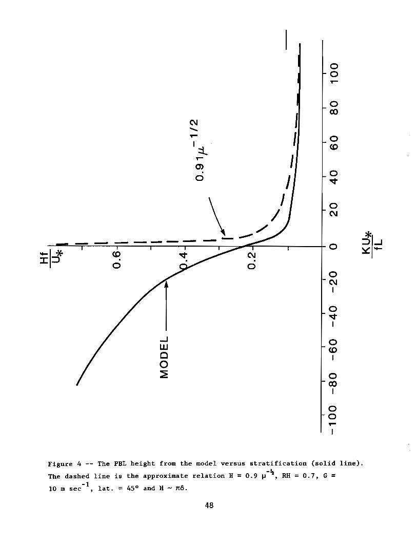
From Paulson's (1970) empirical expression for ~(z/L), model results for PDL

height variation with stratification are shown in Figure 4.

The height of the PDL in stably stratified conditions has often been

written:Hf -!t~ = a~ , (17)*

where ~ = u*/fL and "a" has been found to be from 0.7 to 2, generally

assumed to be near unity. With ~ = -a z/L in stable stratification,o

kn u*

= l±(1-8aOA2~)!t

2a o A

kn

Hf = [(1+0.84~)!t-l]/(I.I~)

when a o = -4.7, k =0.4, and A = 0.15

(18)

In case of large ~, (18) is approximated by 17 with a = 0.8.

While the curve fit (17) breaks down at ~ = 0, (18) has no such problem,

as shown in Figure 4.

Figure 5 shows the effects of stratification on u*, U10

, U19

.5

and a.

Stable stratification has a large effect, and small changes near neutral

result in large change in a and u*. The decreased effect on U19

.5

and U10

compared to u* is evident, a result of the higher level flow being more

influenced by the constant upper boundary condition, G = constant and less

by the layer stratification.

9. THE NEUTRAL DRAG COEFFICIENT AND ROUGHNESS PARAMETER

Under neutral conditions, the wind speed at height z in the atmospheric

surface layer is given by

In(z/z )/k,o

47

(19)

00T-

O

Jro

N"T- I 0I~ WT- Im. 00 I ~

\ J 0

/ N

/*~

0 ~ ~

~I*~~

I~

0NI

0~I

~ 0W W0 I0~ 0

roI

00T-

Figure 4 -- The PBL height from the model versus stratification (solid line).

The dashed line is the approximate relation H = 0.9 ~-\, RH = 0.7, G =-110 m sec , lat. = 45° and H ~ n6.

48

o(\J o

II

oex>

oV

oVI

oex>I

oo(\J

I, \ '. ,\ \ '. ,\ \ :\

\ ,. * I

\

\ ::>1L{). ,

. \ '0), I::> ' ,

\ 0 • "r5 \. "/

~ .. ~ (\J(J) " """"- ..::> , 1---+-/"":""T-7'SI'-=-~----iI---+-~r::',-;-----iI--~ 0EO",,

I \I \I ·I \

, !I !, !

I(J)

*'::> ~ 0q

Figure 5 -=IUI9.5' U10 , u* and a versus stratification. RH = 0.7, lat. = 45°,

G = 10 m s .

49

where Us is the surface drift. The drag coefficient, Cn' relates wind tostress:

(20)

By combining (19) and (20), a relation between Zo and Cn

can be determined:

z = Z (-k/Cn\). (21)o exp

The reference height for Cn

is generally taken to 10 m.

Both the measurements of Nikuradse (1933) on pipe flow and those of

Kondo (1973) at an air-sea interface indicate:

for tU*/1I ~ r1

for r1

~ t U*/1I ~ r2

for r2

~ t U*/II.

(22a)

(22b)

(22c)

Nikuradse (1933) defined t as the actual mean diameter of the sand

grains used as roughness elements and found r1

=5, r2

= 70, G1

= 0.11 and

G2

= 0.03. Kondo (1973) defined t as the root-mean square waveheight for-1

frequencies between 20 and 200 rad/sec and found r1

=5.7, r2

=67, G1

=0.11

and G2

= 0.07. These results separate the flow roughly into smooth,

transition and rough regimes.

For a fully rough air-sea interface, Charnock (1955) obtained by

dimensional reasoning

zo

(23)g

is a constant.zo

constant.-1

is valid; for 3 m s < U10

-1s

gravity and a is a universal-1

s ,(22a)

U10

~ 15 m

where g is the acceleration due to

Wu (1969) found that for U10

< 3 m

< 15 m 8-1

, (23) is valid; and for

50

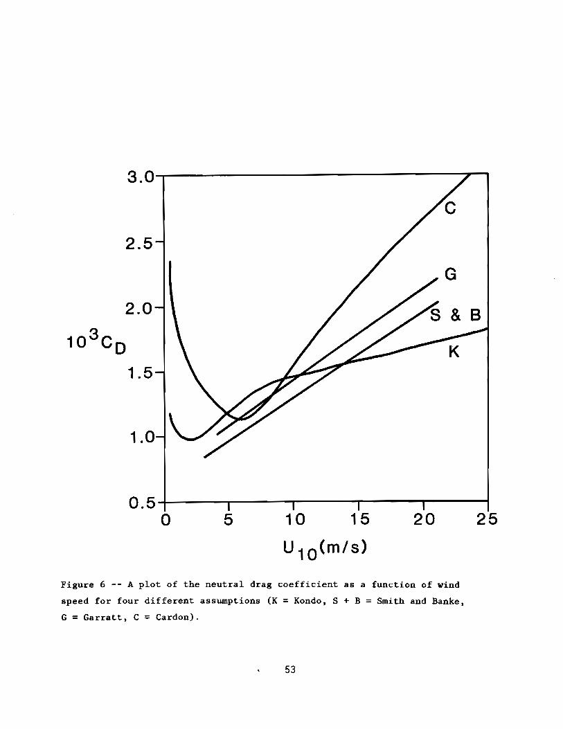
Recently, a number of investigators have obtained empirical relations

between Cn and U10

. Smith and Banke (1975) correlate Cn and U10

for 111

data runs and obtained

10 Cn = 0.63 + 0.066 U10

(24a)

-1for U10 between 3 and 21 m s Garrett (1977) obtained from 18 sets of

data including those of Smith and Banke (.1975)

10 Cn = 0.75 + 0.067 U10

(24b)

-1for U10 between 4 and 21 m s Both (24a) and (24b) agree with (23). Kondo

(1975), by using wind-wave data from Kondo et ale (1973), obtained approximate

relations in the form:

r= p + qU 10 (24c)

that agree with (22). The values of p, q, r for different ranges of wind speed

are shown in Table 4. The difference between Cn given by (24a), (24b) and (24c)

are small for moderate wind speeds. Garratt (1977) did not use the result of

Kondo (1975) to evaluate (24b) but indicated that (24c) agrees well with the

data he collected.

In a boundary layer model proposed by Cardone (1969), a relation is

assumed

(25)

Combining this relation with (21), a relation between CD and U can be obtained.

In evaluating the above relations, the surface drift velocity is neglected

by the investigators, i.e., U is assumed to be zero. The drag coefficient ands

roughness parameter obtained with the U = 0 assumption are related to thes

actual values, Cnand z~,

(26)

(27)

51

The ratio U /u* is a parameter of wind-wave coupling and its effect on thes .

drag has been discussed by Kitaigorodskii (1973) and Davidson (1974). Wu

(1975) found by laboratory experiments that this ratio decreases gradually as

the fetch increases and approaches approximately the relation Us =0.55 u*.

Figure 6 shows the wind-speed dependence of the drag coefficient for

the four models (24a), (24b) , (24c), and (26).

Table 4: Parameters in Expressions for Neutral Bul~ Transfer Coefficients

-1U10 (m s ) p q r

0.3 to 2.2 0 1.08 -0.152.2 to 5 0.771 0.0858 15 to 8 0.867 0.0667 18 to 25 1.2 0.025 125 to 50 0 0.073 1

10. THE STABILITY FUNCTIONS

The surface stress and the surface heat flux can be determined from

U and (T - T ) by integrating the mean profiles.o

U/u* = [In(z/zo) - ~U]/k

(T - To)/T* = [In(z/zo) - ~T]/aNk,

(28)

(29)

where T* = -Ho(cpu*), aN =~/~ at neutral stability, ~ and ~ are the

turbulent diffusivities for heat and momentum, c is the isobaric specific

heat, U and T are the mean wind speed and potential temperature at height z,

and T is the temperature at z given by the extrapolation of (29). The0 0

evaluation of z has been discussed in section 9. In this section we0

investigate the stability functions ~U and ~T.

For a diabatic surface layer, similarity theory suggests that the non­

dimensional gradients are functions of the stability parameter, t.

52

252010 15

U 1O(m/s)

5

3.0--------------~...,

1.0

0.5-+-----.-----r----r-----,...----!

o

2.5

Figure 6 -- A plot of the neutral drag coefficient as a function of wind

speed for four different assumptions (K =Kondo, S + B = Smith and Banke,

G = Garratt t C = Cardon).

53

where t = z/L1

and L is the Obukhov's length. Combination of (28), (29), (30)

and (31) gives

~U = Ifo[(1 - ~U)/t')Jdt'

~T = f~o[(1 - ~T)/t')Jdt'.

Under unstable conditions, the KEYPS model (Panofsky et al., 1960) proposes

(32)

The adjustable constant a is taken to be 18 following Panofsky et al. (1960).

If the effect of moisture fluctuations on density is neglected, the

Obukhov's length is defined as

(33)

With the assumption that ~/~ is constant and equal to unity, ~T = ~U = ~,

~ =~ =~ andT U

(34)

Recently, profile measurements in the surface layer have been success­

fully described by the Businger-Dyer model:

(35)

(36)

INote a new definition for t.

54

Results from the Kansas experiment (Businger et al., 1971) give aU = 15, aT

= 9 while k = 0.35 and aN = 1. However, Paulson (1970), with the assumption

that k = 0.4 and aN = 1, obtained aU = aT = 16 in his analysis of Kerang

data, in close agreement with Dyer (1967). The Businger-Dyer model differs

from the KEYPS model in that the B-D model allows for the variation of ~/KM

with stability. Paulson (1970) found that both models describe velocity

distribution equally well but the B-D model gives better representation in

temperature distribution. The two models also give different dependence

of U and T on z when free convection is approached (see Businger et al.,

1971 and Businger, 1973 for further discussion). Both the Kansas and

Kerang data are measured over land. The B-D model has also been found to

represent measurements over ocean in the Spanish Bank experiment (Miyake

et al., 1970), the Indian Ocean experiment (Badgley et al., 1972), and

the BOMEX experiment (Paulson et al., 1972).

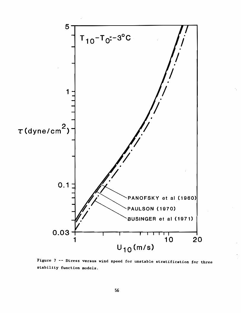
Figure 7 shows the stress as a function of wind speed for unstable

stratification of 3°C for the three models. zo(u*) relations from Cardone

(1969) have been used in these calculations. Figure 8 shows the rate of

heat flux evaluated for a range of air-sea temperature differences. T10

a~d U10

are potential temperature and wind speed at 10 m. Stresses evalu­

ated with the B-D model with k = 0.4 are about 1 percent lower than those

evaluated with the KEYPS model at moderate wind speed but increase to 8 per--1

cent at 1 m s wind. With k = 0.35 the stress is about 30 percent lower.

The heat fluxes evaluated by the B-D model with the two sets of constants are

about 6 and 13 percent lower than those with the KEYPS model.

Under stable conditions, the log-linear model which was obtained by dropping

the higher order terms in the power expansion of ~U and ~T are used:

(37)

Cardone (1969) uses the values k =0.4, aN = 1, bT = bU = 7. Similar

values have been used by McVeil (1963) and others. Businger et al. (1971)

suggested k = 0.35, aN = 1.35, bU = 4.7 and bT = 6.35. However, the log-

55

5

1

2T (dyne/em )

0.1

PANOFSKY at al (1960)

PAULSON (1970)

BUSINGER at al (1971)

1010.03 4----,...---r---"""T"""'""~__r_t_.__--_;

20

Figure 7 -- Stress versus wind speed for unstable stratification for three

stability function models.

56

U 10 4m/s

PANOFSKY (1960)

BUSINGER et al (1971)

PAULSON (1970)

5

2

3

7

6

1

8--r---------------.".,

H2 4(mw/cm )

o -;-----r----..,----r-----I

Figure 8 -- Heat flux as a function of unstable air sea temperature for

three stability models.

57

linear model has its limitations. From the definition,

where Ri = 2g(8T/8z) is the Richardson number.

t = A1 + B'

where A =a~i, B =a~i band t can be solved by fix-point iterations only

if

B < 1

and

RI." < ( b)-1aN . (39)

-1The quantity (aNb) is also the asymptotic value of Ri as t increases in

value.

The criterion (39) is equivalent to

1, b = 7, T = 280oK, in order to have

x 10-5 . In other words, there is no-1

= 1°C and when Uto < 221 em s

-1For z = 10 m, g = 981 cm s ,aN =

a realistic solution, (T - TO

)/U2 < 4.1-1

solution when U10 < 157 cm s for (T10 - TO)

for (T10 - TO) = 2°C. Kondo (1975) suggested

~ = 1 + 6t/(1 + t), (40)

which is not subjected to the above condition for a solution.

The stresses evaluated with these models are compared in Figure 9.

The stress evaluated with Cardone (1969) is lower than that evaluated with-1

Kondo's model by 3 percent at a wind speed of 10 m s and by 59 percent at-1

a wind speed of 2 m s . With the representation suggested by Businger

et al. (1971), which means a different value of von Karman's constant, the

stress is about 40 percent lower than the Kondo representation. Most of

this is due to the smaller k.

58

30 -r-------------'T,----,

,

'f:;KONDO (1975)

if BUSINGER at 81 (1971)

~CARDONE (1969)

1

0.1

1 10U10 (m/s)

20

Figure 9 -- Stress versus wind speed for stable stratification for three

stability function models.59

Over water, the effect of moisture fluctuations on buoyancy may be

important. The Obukhov length can be redefined to include this effect:

where Tv = T(l + 0.61Q) and Tv* = T*(l - 0.61Q) + 0.61~, ~ = -E/u*, E is

the moisture flux, Q is the specific humidity at z. The moisture flux can

be determined from the humidity profile

where aN' = KE/~ at neutral stability and KE is the turbulent diffusivity

of moisture. Assuming aN' =aN' ~Q =~T' the stress and heat flux can be

evaluated for different values of relative humidity. The percentage differ­

ence between the values evaluated with the effects of moisture included and

those with the effects excluded are shown in Tables 5 and 6. The difference

in stress decreases with increasing wind speed because at low wind speed the

buoyancy production becomes increasingly important relative to the shear

production. The difference is larger the drier the air.

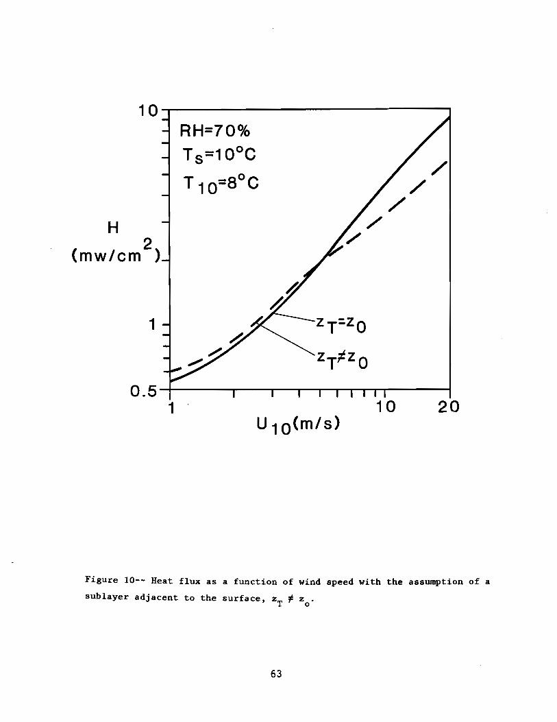
The sea-surface temperature T , rather than T , is generally available.s 0

Figure 10 shows that under slightly unstable conditions, the heat flux

Ts(ZT = zo) differs from those extimated by

(Liu, 1978) by 3 percent in low wind speed up to

extimated by assuming T =o

including a sublayer model-1

27 percent for 20 m s winds.

60

Table 5: Percentage Difference Between the Stress Evaluated with theEffects of Moisture on Buoyancy Included and those with theEffects Excluded.

TO = 10°C

T10 - TO = 1°C T10 - TO = -3°C

R.H. R.H.

U10

(m -1100% 60% 0% 60% 0%s ) 100%

1 20 64 159 1 4 6

5 1 6 18 1 2 3

10 0.3 2 7 1 1 4

T = 25°C0

T10 - TO = 1°C T10 - TO = -3°C

R.H. R.H.

-1100% 60%U

10(m s ) 0% 100% 60% 0%

1 13 5 169 3 8 14

5 -0.3 17 4 2 4 8

10 -8 7 10 1 5 12

61

Table 6: Percentage Difference Between the Heat Flux Evaluated with

the Effects of Moisture on Buoyancy Included and those with-1the Effects Excluded (U10 = 5 m s )

T =100 e TO =25 0 e0

R.H. R.H.

T10 -TO 100\ 60\ 0\ 100'%. 60\ 0\

-3 0 e 1 2 3 2 4 7

l oe 1 7 8 -0.3 18 28

62

//

//

/

RH=70%Ts =10oC

T 10=8°C

1 zT=zO

zT~zO

0.51 10 20

U 10(m/s)

10-------------.....,

H2

(mw/cm )

Figure 10-- Heat flux as a function of wind speed with the assumption of a

sublayer adjacent to the surface, zT ~ zoo

63

REFERENCES (APPENDIX A)

Badgley, F. I., C. A. Paulson and M. Miyake (1972): Profile of wind

temperature and humidity over the Arabian Sea, International Indian

Ocean Expedition. Meteor. Monograph, 6, 66.

Brown, R. A. (1970): A secondary flow model for the planetary boundary

layer. J. Atmos. Sci., 27, 742-757.

Brown, R. A. (1972): The inflection point instability problem for stratified

rotating boundary layers. J. Atmos. Sci., 29, 850-859.

Brown, R. A. (1974): Analytical Methods in Planetary-Layer Modelling, Adam

Hilger Ltd., London, and Halsted press, John Wiley & sons, N. Y. 148 pp.

Brown, R. A. (1978): Similarity parameters from first-order closure and data.

Boundary-Layer Meteorol., 14,381-396.

Businger, J. A. (1973): A note of free convection. Boundary-layer Meteorol.,

4, 323-326.

Businger, J. A., J. C. Wyngaard, Y. Izumi and E. F. Bradley (1971): Flux

profile relationships in the atmospheric surface layer. J. Atmos.

Sci., 28, 181-189.

Cardone, V. J. (1969): Specification of the wind distribution in the marine

boundary layer for wave forecasting. Report GSL-TR69-1, New York Univ.,

School of Engineering and Science, 131 pp.

Charnock, H. (1955): Wind stress on a water surface. Quart. J. Royal Meteor.

Soc., 81, 639-640.

Davidson, K. L. (1974): Observational results on the influence of stability

and wind-wave coupling on momentum transfer and turbulent fluctuations

over ocean waves. Boundary-Layer Meteorol., 6, 305-331.

64

Dyer, A. J. (1967): The turbulent transport of heat and water vapour in an

unstable atmosphere. Quart. J. Roy. Meteor. Soc., 93, 501-508.

Garrett, J. R. (1977). Review of drag coefficients over oceans and continents.

Mon. Weather Rev., 105, 915-929.

Hasse, L. (1970): On the determination of vertical transports of momentum and

heat in the atmospheric boundary layer at sea. Technical Report 188,

School of Oceanography, Oregon State University.

Kitaigorodskiy, S. A. (1973). The Physics of Air-sea Interaction, Israel

Program for Scientific Translation, Jerusalem.

Kondo, J. (1975): Air-sea bulk transfer coefficients in diabatic condition,

Boundary-Layer Meteorol., 9, 91-112.

Kondo, J., Y. Fujinawa and G. Naito (1973): High frequency component of

ocean waves and their relation to aerodynamic roughness. J. Phys.

Oceanogr., 3, 197-222.

Liu, W. T. (1978): The molecular effects of air-sea exchanges. Ph.D.

dissertation, University of Washington, Seattle.

Liu, W. T. and J. Businger (1975): Temperature profile in the molecular

sublayer near the interface of a fluid in turbulent motion. Geophys.

Res. Let., 2, 403-404.

Liu, W. T., K. B. Katsaros and J. A. Businger (1979): Bulk parameterization

of air-sea exchanges of heat and water vapor including the molecular

constraints at the interface, submitted to J. Atmos. Sci. for

publication.

McVeil, G. E. (1964): Wind and temperature profiles near the ground in stable

stratification. Quart. J. Roy. Meteor. Soc., 90, 136-146.

65

Miyake, M., M. Donelan, G. McBean, C. Paulson, F. Badgley and E. Leavitt

(1970): Comparison of turbulent fluxes determined by profile and eddy

correlation techniques. Quart. J. Roy. Meteor. Soc., 96, 132-137.

Nikvradse, J. (1933): Laws of flow in rough pipes, N.A.C.A. Technical

Memorandum 1292.

Paulson, C. A, (1970): The mathematical representation of wind speed and

temperature profiles in the unstable atmospheric surface layer.

J. Appl. Meteorol., 9, 857-861.

Paulson, C. A., E. Leavitt and R. G. Fleagle (1972): Air-sea transfer of

momentum, heat, and water determined from profile measurements during

BOMEX. J. Phys. Oceanogr., 2, 487-497.

Panofsky, H. A., A. K. Blackadar and G. E. McVeil (1960): The diabatic wind

profile. Quart. J. Roy. Meteor. Soc., 86, 390-398.

Smith, S. D. (1973): Thrust-anemometer measurements over the sea reexamined,

Report 73-1, Bedford lnst. Oceanography.

Smith, S. D. (1974): Eddy flux measurements over Lake Ontario. Boundary­

Layer Meteor., 6, 235-256.

Smith, S. D. and E. G. Banke (1975): Variation of the sea surface drag

coefficient with wind speed. Quart. J. Roy. Meteor. Soc., 101,665-673.

Wu, J. (1969): Wind stress and surface roughness at the air-interface. J.

Geophys. Res., 74, 444-455.

Wu, J. (1975): Wind-induced drift currents. J. Fluid Mech., 68, 49-70.

Wu, J. (1979): Wind-wave interaction. Phys. Fluid, 13, 1926-1930.

66

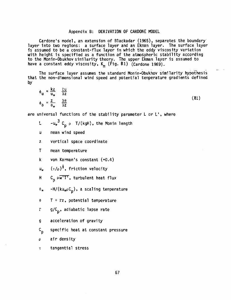
Appendix B: DERIVATION OF CARDONE MODEL

Cardone's model, an extension of Blackadar (l965), separates the boundary'layer into two regions: a surface layer and an Ekman layer. The surface layeris assumed to be a constant-flux layer in which the eddy viscosity variationwith height is specified as a function of the atmospheric stability accordingto the Monin-Obukhov similarity theory. The upper Ekman layer is assumed tohave a constant eddy viscosity, ~ (Fig. 81) (Cardone 1969).

- -The surface layer assumes the standard Monin-Obukhov similarity hypothesis

that the non-dimensional wind speed and potential temperature gradients defined~ .

c/> =g 2uu u* ClZ

c/> =L de(B1 )

e e* ClZ

are universal functions of the stability parameter L or LI, where

3L -u* Cp p T/{kgH), the Monin length

u mean wind speed

z vertical space coordinate

T mean temperature

k von Karman's constant (=O.4)

u* (T/P)!' friction velocity

H Cp ~w'T', turbulent heat flux

e* -H/{kU*pCp)' a scaling temperature

e T + rz, potential temperature

r g/Cp' adiabatic lapse rate

g acceleration of gravity

Cp specific heat at constant pressure

p air density

T tangential stress

67

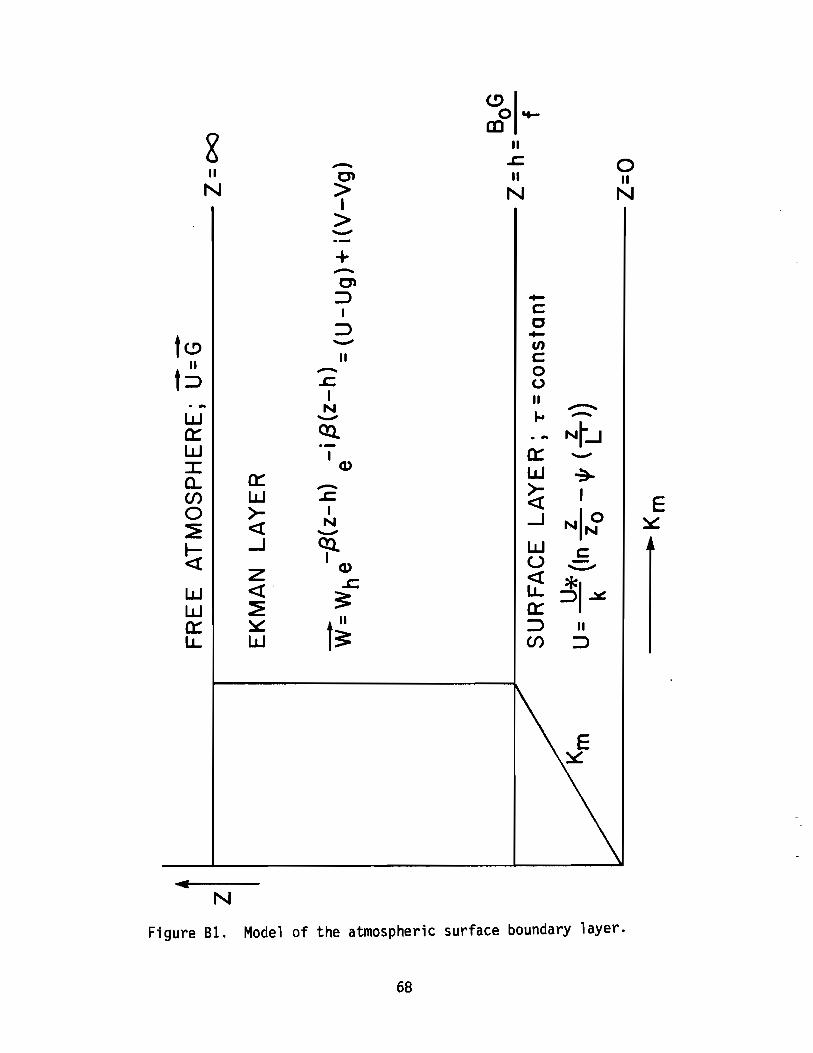
(!)0 .....

&CD

II- ~ 0II C\ II IIN > N N

I>-+-C\:::> +-

I c::::> c

t(!) +-- en

t;II c:- 0

.c 0I II. .. N

W......-...- "" -a::: co. . .. N~...J

W I a::: -:r: Q) w ,.a.. a::: - >-(/) W ~ Ia >- I «

NI~E

~ « N ...J ~-~ ...J ep. W« u c:

ZQ) ~

.c «31~w «' 3= IJ...

W ~ a:::a::: ~ t~

:::> II

IJ... W (/) :::>

...N

Figure B1. Model of the atmospheric surface boundary layer.

68

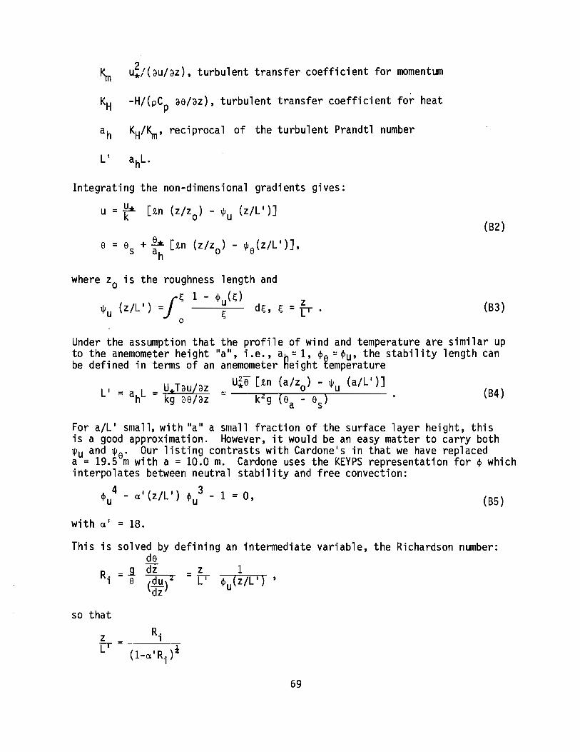
~ u;/{au/az), turbulent transfer coefficient for momentum

KH -H/{pCp aa/az), turbulent transfer coefficient for heat

ah KH/~, reciprocal of the turbulent Prandtl number

Integrating the non-dimensional gradients gives:

u =~ [2n (z/zo) - ~u (z/l')](B2)

where Zo is the roughness length and

ft; 1 - cI> (t;) _ z

~u (z/l') = ~ dt;, t; - [' •o

(B3)

(B4)II = a l = U*Tau/az '"h kg'[)alaz

Under the assumption that the profile of wind and temperature are similar upto the anemometer hei ght "a", i.e., ah'" 1, cl>e '" cl>u' the stabi 1ity 1ength canbe defined in terms of an anemometer height temperature

U~e [2n (a/zo) - ~u (all')]kZg (aa - as)

(B5)

For all' small, with "a" a small fraction of the surface layer height, thisis a good approximation. However, it would be an easy matter to carry both~u and ~a· Our listing contrasts with Cardone's in that we have replaceda = 19.5 mwith a = 10.0 m. Cardone uses the KEYPS representation for cI> which"j nterpo1ates between neutral stab"' 1ity and free convecti on:

cl>u4 - a l (z/l') cl>u3 - 1 = 0,

with a I = 18.

This is solved by defining an intermediate variable, the Richardson number:da

R. = ~ dZ _ z 1, e (du)z - [' -cI>-'("';;;'z""""/l-:"-'-) ,

dz u

so that

69

and1

~ = ~ .u (l _ a'R.)'l,

The KEYPS representation implies that bothu and e vary asymptotically as z-1/3.The B5 relation implies

~(z/L') = 1-.-31n~ + 21n(1 ; ~) + 2tan-1~- ¥+ In(l ; .2). (B6)

An alternate form.is the Businger-Dyer {B-D) profiles:

• = [1 - a'(z/L)]-iu

.e = [1 - a'(z/L)]-l

~u = 21n [(1 + x)/2] + In [(1 + x2)/2] - 2 tan-1 x + %

~e = 21n [(1 + x2)/2],

where x = (1 - a'z/L)i •(B7)

The ~e profile is important only to level lI a ll (i .e., in defining L'); however,the choice of the ~u profile is critical in matching velocities at the top ofthe surface layer. For stable boundary layers, Cardone has

.u (z/L') = 1 + S'z/L'

~u (z/L') = -S'z/L '

with SI = 7.

(B8 1)

The linear profile in B81 is generally limited to z/L' < 0.3 which in practicecan be ea - es < 2°C. To extend the stable range we replace B8 1 by

• (z/L') = 1 + S'(z/L ' )u 1 + z/L '

(B8)~ (z/L') = -SI In(l + z/L').

Wave development is considered indirectly through the dependence of surfaceroughness upon u* in the following relation:

-5 2 -2Zo =0.684/u* + 4.285 x 10 u* - 4.43 x 10 , (B9)

where z is in cm and u* in cm s-l. The relation B9 implies a viscous sub­layer f8r small u* and the Charnock (1955) relation (zo = acu*2/g) for large u*.

70

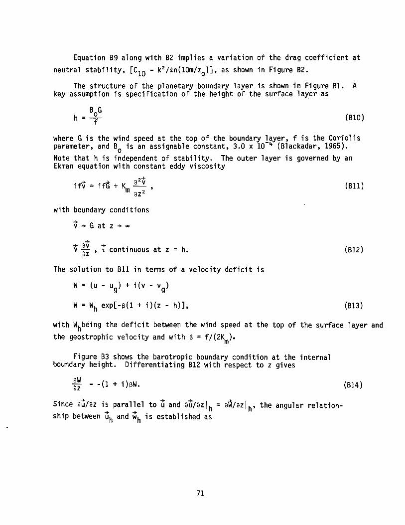
(B10)

Equation B9 along with B2 implies a variation of the drag coefficient atneutral stability, [C10 = k2 /tn(10m/zo)]' as shown in Figure B2.

The structure of the planetary boundary layer is shown in Figure B1. Akey assumption is specification of the height of the surface la~er as

BoGh =f

where G is the wind speed at the top of the boundary layer, f is the Coriolisparameter, and Bo is an assignable constant, 3.0 x 10-4 (Blackadar, 1965).Note that h is independent of stability. The outer layer is governed by anEkman equation with constant eddy viscosity

(B11)

with boundary conditions+v + G at z + 00

+ av + .v az ' L cont,nuous at z = h.

The solution to B11 in terms of a velocity deficit is

W= (u - ug) + i(v - vg)

W=Wh exp[-a(l + i)(z - h)],

(B12)

(B13)

with Whbeing the deficit between the wind speed at the top of the s,urface layer andthe geostrophic velocity and with a = f/(2K ).

m

Figure B3 shows the barotropic boundary condition at the internalboundary height. Differentiating B12 with respect to z gives

~~ = -(1 + i)aW. (B14)

Since du/az is parallel to u and au/azlh = aW/azlh, the angular relation­ship between uh and ~h is established as

71

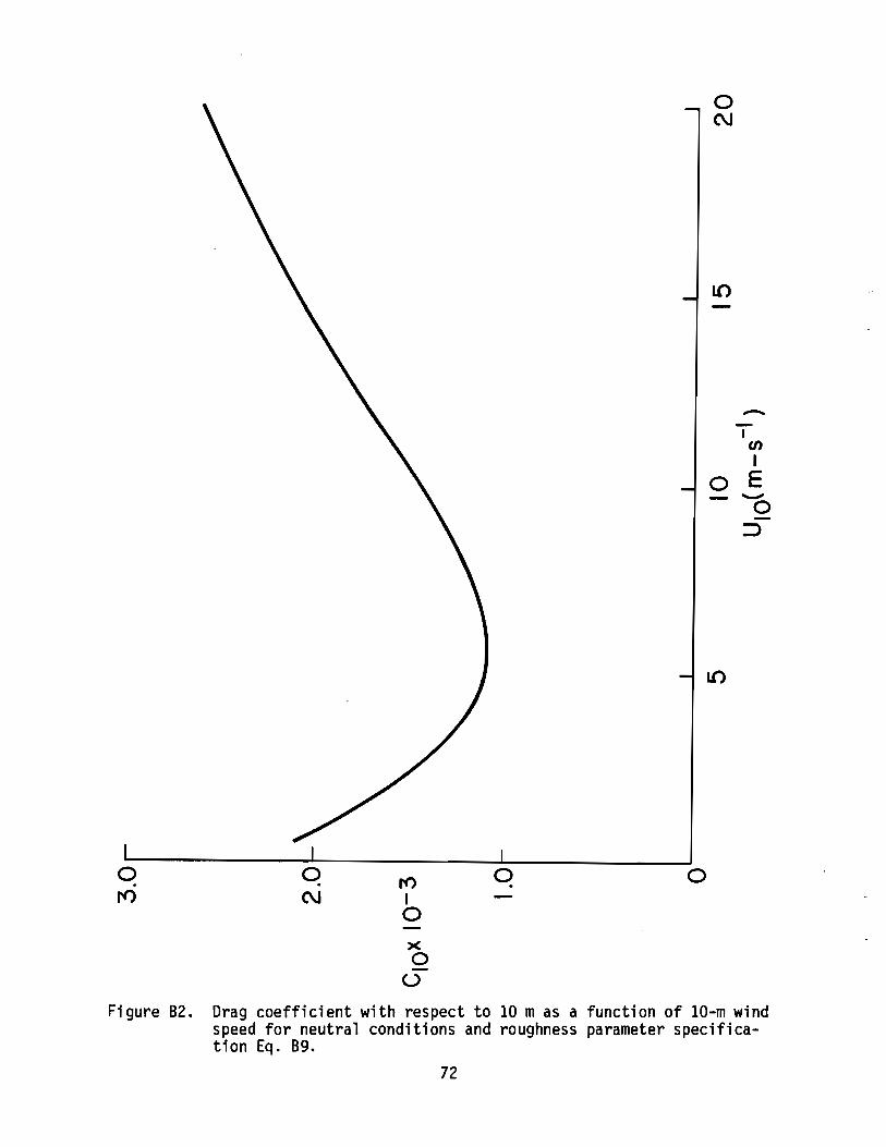
oN

I~

Io E~o~

0 0~

0 0~ N I

0x0

UFigure B2. Drag coefficient with respect to 10 m as a function of 10-m wind

speed for neutral conditions and roughness parameter specifica­tion Eq. B9.

72

Figure B3. Barotropic boundary condition on the internal boundary surface.

73

(BI5)

By using the law of sines on Figure B3

(BI6)

and again

The profile Bl in the surface layer implies

K - k u. z h'111 - ~u (zlL I ) z $ •

This relation combined with BI0 and B12 implies

k u* BoG~ = f~ (Z/li) Z ~ h

u

and

(BI7)

(BI8)

(BI9)

(B20)

The mixing coefficient in the upper layer is a function of stability in thesense that its magnitude is determined by the value where the profile B18intersects height h and is larger for unstable stability and smaller for astable regime. At z = h

u BoGuh =k [R.n h - 1/Ju(h/l')] (B21)

a

au u*f~u(h/l')-I = (B22)az -h k BoG

B22 and B23 imply

IWhj= u*f <Ilu(h/l')/(A k BoG a).

74

(B23)

(B24)

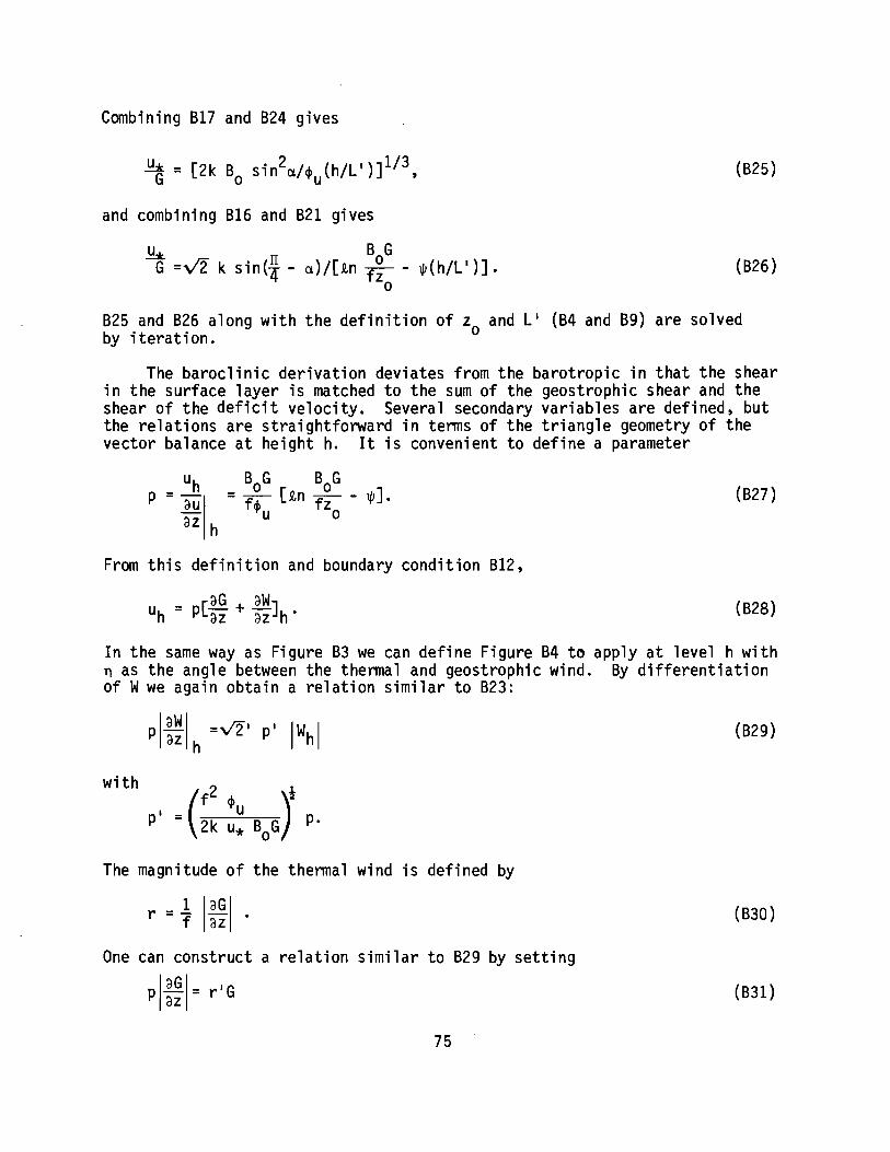
Combining B17 and B24 gives

and combining B16 and B21 gives

.!!:t. . II B GG=~ k s1n(4 - a)/[~n f~ - ~(h/L')J.

o

(B25)

(B26)

B25 and B26 along with the definition of z and L' (B4 and B9) are solvedby iteration. 0

The baroclinic derivation deviates from the barotropic in that the shearin the surface layer is matched to the sum of the geostrophic shear and theshear of the deficit velocity. Several secondary variables are defined, butthe relations are straightforward in terms of the triangle geometry of thevector balance at height h. It is convenient to define a parameter

From this definition and boundary condition B12,

_ [aG + aWJuh - p az az h'

(B27)

(B28)

In the same way as Figure B3 we can define Figure B4 to apply at level h withn as the angle between the thermal and geostrophic wind. By differentiationof Wwe again obtain a relation similar to B23:

The magnitude of the thermal wind is defined by

r = 1 I~I .f az

One can construct a relation similar to B29 by setting

pl~~I= riG

75

(B29)

(B30)

(B31)

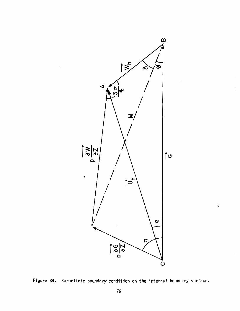
m

a. //

//

/

//

~/

/

,

Figure 84. 8aroclinic boundary' condition on the internal boundary surface.

76

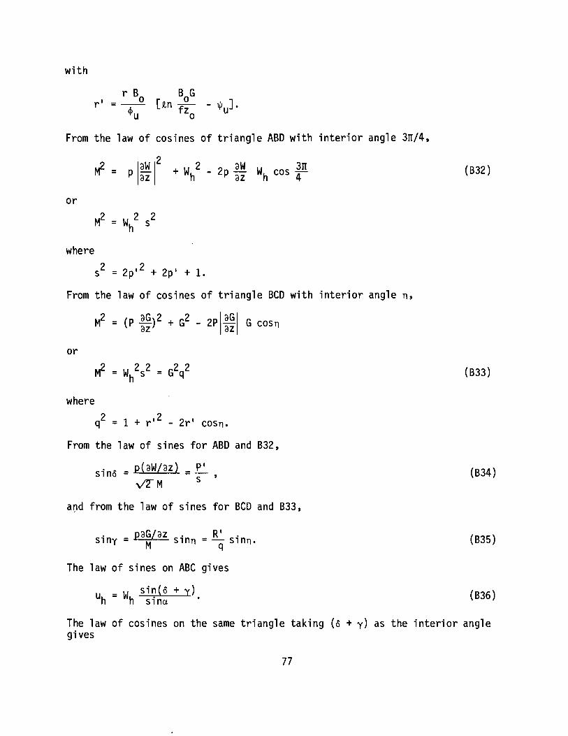
with

From the law of cosines of triangle ABD with interior angle 3rr/4,

or

where

s2 = 2p·2 + 2p' + 1.

From the law of cosines of triangle BCD with interior angle n,

M2 = (P ~)2 + G2 _ 2plaGI G COSnaz az

or

where

q2 = 1 + r ,2 - 2r ' COSn.

From the law of sines for ABD and B32,

sino = p(aw/az) =.~ ,vTM s

a~d from the law of sines for BCD and B33,

. paG/az. RI •

Slny = M Slnn = -q Slnn·

The law of sines on ABC gives

u - W sin(o + y)h - h sina .

(B32)

(B33)

(B34)

(B35)

(B36)

The law of cosines on the same triangle taking (0 + y) as the interior anglegives

77

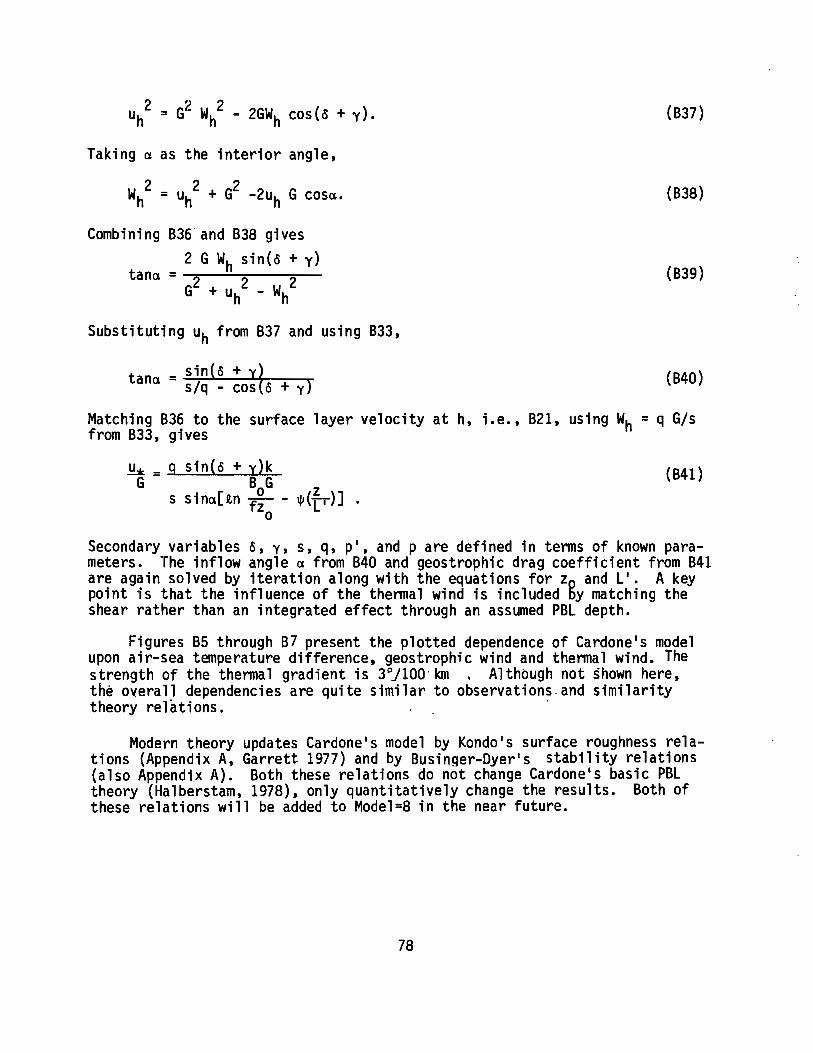
222uh = G Wh - 2GWh cos{~ + y).

Taking a as the interior angle,

222Wh = uh + G -2uh G COSa.

Combining 836' and 838 gives2 G Wh sin{~ + y)

tana = 2 2 2G + uh - Wh

(837)

(838)

(839)

(840)

SUbstituting uh from 837 and using 833,

t n - sin{~ + Y~a a - s/q _ cos ~ + y}

Matching 836 to the surface layer velocity at h, i.e., 821, using Wh = q G/sfrom 833, gives

(841)

Secondary variables ~, y, s, q, pi, and p are defined in terms of known para­meters. The inflow angle a from 840 and geostrophic drag coefficient from 841are again solved by iteration along with the equations for Zg and Lt. A keypoint is that the influence of the thermal wind is included y matching theshear rather than an integrated effect through an assumed P8l depth.

Figures 85 through 87 present the plotted dependence of Cardone's modelupon air-sea temperature difference, geostrophic wind and thermal wind. Thestrength of the thermal gradient is 3°J100'km • Although not shown here,the overall dependencies are quite similar to observations. and similaritytheory relations. .

Modern theory updates Cardone's model by Kondo's surface roughness rela­tions (Appendix A, Garrett 1977) and by 8usinger-Dyer ' s stability relations(also Appendix A). 80th these relations do not change Cardone's basic P8ltheory (Ha"lberstam, 1978), only quantitatively change the results. 80th ofthese relations will be added to Model=8 in the near future.

78

L-----l----------+--------+---Jr-"TTT----j'"~------+---+----__:____+_____fJ_____J/~'1J~ '"~---l----1---_____+______;_I___tI_tt·1 J------, ...1---___l_--_1_--_____+---.,.I----jJi-?-r;-t-J------, M

l---~--__+__--~y~~-;;--'l-r-/-~ C\l

~~/

/ II I/ II '

/ III/ V

I EICil r1-----+--4-----g j EICIl---_-+__+- --l

~ICfl I ~-4-4~~----___4--+-------__;:1 / ~7 ~ ~,!")t: I T11:

0

";" ()0

~

<:'Q,)CIlI-

l"? "(ij

l-

t--"

'r<2

":'

'i'

";-

'l'

~ ~I" ~ ~ ~Figure B5. Dependence of the geostrophic drag coefficient on ~he air-sea tem:

1perature difference from Cardone's model. Two curves are glven for 15 m sand 30 m s- geostrophic wind and barotropic conditions. The high and lowcurves are for two orientations of the thermal wind for a surface air temper­ature gradi ent of 3°C /100 km.

79

~

I

o

MI

II)

!iil II)~

" "C) C)

~M0 0 l=IM" " "

" c: c: c:-~ I ,n T

I J

III {) ~ 4 \\.

/ \,~.....

~

/ \ \ "J., ,

~•

/ \/ \

! \I '\

I

I ,I

11,

!iil I II) I~ II)

I o I I I I I 0 II .- .-(\j - ... II)

Figure B6. A similar set of curves as in AS for inflow angle.

80

E EE.JIf. .JIf.

8 8 .JIf.0

~~ 0 t, ,

~. . , s:0 ~ .C'? ~ 0

II II

l- I- l-

t£> t£> tt>

II)

r-------..:;lIrt...:=::.....---~--+-------+-------...j.~,

r-------+---------+---::...,....:::::::::......-----I----------+~

r-------+---------+-----~:.....-+_--~l::::...--__I_§I

Figure 87. Influence of orientation of the thennal wind on inf10w angle forthree magnitudes of the thennal wind, 0, 1.5° and I3°C/I00 km from Cardone'smodel. The geostrophic wind magnitude is 15 m s- .

81

REFERENCES (APPENDIX B)

Blackadar, A.K.(1965): A simplified two-layer model of the baroclinic neutralatmospheric boundary layer. Air Force Cambridge Res. Lab. Report 65-531,pp 49-65.

Cardone, V.J.(1969): Specification of the wind distribution in the marineboundary .layer for wave forecasting. Reeort GSL-TR69-1, New YorkUniversity, School of Engineering and SClence, 131 pp.

Charnock, H.(1955): Wind stress on a water surface. Quart. J. R. Met. Soc.,81, 639-640.

Garrett, J.R. (1977): Review of drag coefficients over oceans and continents.Mon. Wea. Rev." 105, 915-929.

Halberstam, I. (1978): The marine surface layer and its relationship to Seasat-AScatterometer measurements. Jet Propulsion Laboratory (unpublished manuscript).

82