methods correcting for multiple testing: operating characteristics

* Correspondence to: Barry W. Brown, Department of Biomathematics, 1515 Holcombe Boulevard, The University ofTexas M.D. Anderson Cancer Center, Houston, TX 77030, U.S.A.s Kathy Russell is now at User Services: MS 119, Rice University, 6100 South Main, Houston, TX 77005, U.S.A.

Contract grant sponsor: National Cancer InstituteContract grant number: CA 16672

CCC 0277—6715/97/222511—18$17.50 Received May 1996( 1997 by John Wiley & Sons, Ltd. Revised February 1997

STATISTICS IN MEDICINE, VOL. 16, 2511—2528 (1997)

METHODS CORRECTING FOR MULTIPLE TESTING:OPERATING CHARACTERISTICS

BARRY W. BROWN* AND KATHY RUSSELLs

Department of Biostatistics, Box 237, 1515 Holcombe Boulevard, The University of Texas M. D. Anderson Cancer Center,Houston, TX 77030, U.S.A.

SUMMARY

We examine the operating characteristics of 17 methods for correcting p-values for multiple testing onsynthetic data with known statistical properties. These methods are derived p-values only and not the rawdata. With the test cases, we systematically varied the number of p-values, the proportion of false nullhypotheses, the probability that a false null hypothesis would result in a p-value less than 5 per cent and thedegree of correlation between p-values. We examined the effect of each of these factors on familywise andfalse negative error rates and compared the false negative error rates of methods with an acceptablefamilywise error. Only four methods were not bettered in this comparison. Unfortunately, however,a uniformly best method of those examined does not exist. A suggested strategy for examining correctionsuses a succession of methods that are increasingly lax in familywise error. A computer program for thesecorrections is available. ( 1997 by John Wiley & Sons, Ltd.

Statist. Med., 16, 2511—2528 (1997)No. of Figures: 4 No. of Tables: 2 No. of References: 21

1. INTRODUCTION

Multiple hypothesis tests are common in biomedical trials. In a comparative trial, differentialeffects are examined by overlapping groups of subjects, for example by sex, age, and stage ofdisease. These multiple examinations are likely to continue as long as the cost of obtaining andanalysing additional information about subjects already enrolled in a trial is much less than thatof mounting new trials. Sometimes, an overall comparison of two treatments yields a negativeresult, while some subgroups show an apparently significant difference. The statistician mustdetermine whether these subgroup differences are worthy of further investigation or whether theyare not surprising given the number of hypotheses examined.

Multiple hypothesis tests are sometimes performed to avoid very complex analyses whoseresults would be difficult to communicate, and for which the requisite methodology may not exist.For example, in a comparative trial of two palliative treatments for symptomatic expression of

a fatal disease, measurements of improvement are taken at regular time intervals. Subjects dropout of the trial because of death, so the measurements are available on successively smallergroups. A separate analysis of subjects still on study at each time might well be conducted insteadof using a repeated measures model with informative censoring.

In analysing data, investigators frequently ignore the number of hypothesis tests performed,a practice that inflates the probability of obtaining false positive results. Methods of dealing withthe inflation in the number of apparently significant results because of multiple testing aresurveyed in monographs by Miller1 and Hochberg and Tamhane.2 A compendium of bootstrapcorrection methods is provided by Westfall and Young.3 The first chapter of the latter referencesurveys the philosophical issues associated with this problem. Proschan and Follman4 cogentlydiscuss the need for corrections in comparing several treatments with a single control. Thecontinuing interest in correcting for multiplicities in biomedical research is shown in a recentarticle by Aickin and Gensler5 and the accompanying editorial.

We investigate the operating characteristics of 17 corrections for multiplicity by examiningtheir performance on data sets of known composition. The methods examined use only p-valuesand not the raw data, a choice that excludes bootstrap methods, for example. All of these methodsuse the configuration of the p-values, so it is difficult to use these methods to adjust sample-sizerequirements in designing a study.

We use the traditional criterion for acceptability of a correction methods, its familywise errorrate (FWE), which is the probability of any false positive result. However, Benjamini and Hoch-berg6 argue that in some cases, the less-restrictive criterion of controlling the false positive rate ismore appropriate. Based on this criterion, they recommend the U.sm method described below. Theperformance of an acceptable correction method is measured by its false negative error rate (FNE).

Mathematical guarantees of the properties of corrections for multiple testing usually requireassumptions that frequently are not met and that cannot be verified. Testing is necessarily limitedin scope and so can never provide a guarantee, although it can demonstrate unacceptablebehaviour. Although both the mathematics and the testing may provide reassurance, correctingfor multiple testing must be considered largely exploratory.

1.1. Reader’s guide to this paper

Section 2 describes the several classes of methods tested. Particular methods are detailed inAppendix I; these details are deferred from the text because we tested 17 methods and recallingeach requires considerable effort. Section 3 reports the test cases used. In Section 4, the effects ofthe parameters of the test cases on error rates are recounted; this section treats the variousmethods as interchangeable. Section 5 provides a comparison of all the methods found to haveless than 20 per cent FWE in all test cases, and Section 6 contains recommendations for use basedon this comparison. Readers may wish to examine the details of recommended methods afterhaving read Sections 5 and 6. A computer program that performs the various corrections formultiplicity is announced in Section 7. Appendices II—IV contain the algorithms used formethods that require more than the simple evaluation of a formula.

2. CLASSES OF METHODS

Let the set of p-values sorted in ascending order be pi"1,2 , n, and let the null hypothesis

corresponding to pi, be H

i. The methods considered reject only those hypothesis with the smallest

p-values; they differ only in the number of hypotheses rejected.

SIM 693

2512 B. BROWN AND K. RUSSELL

Statist. Med., 16, 2511—2528 (1997) ( 1997 by John Wiley & Sons, Ltd.

Methods for correcting for multiple testing are categorized as one-step, step-down (D), step-up(U), graphic, mixture (M), or composite types (C). The letters in parentheses are the first letters inthe mnemonic for each method; the remainder of the mnemonic specifies the particular method inthe class. We describe all methods in Appendix I.

We did not test one-step methods, since step-down methods provide equal protection withbetter FNE rates. The graphic method provides an estimate of the number of interesting results,an estimate used in the composite methods. However, the graphic method itself does not providea means of correction, so we have not tested it.

2.1. One-Step Methods

One compares all p-values with a value calculated from a and n, and one rejects null hypotheseswith p-values smaller than this value.

2.1.1. Bonferroni Adjustment

Reject Hiif

p@i"np

i)a.

2.1.2. S[ ida& k Adjustment

The adjustment8,9 rejects Hiif

p@i"1!(1!p

i)n)a.

The adjustment is exact if the ps are independent and uniformly distributed on (0,1); thetransformed value is the probability that the smallest of the n p-values does not exceed p.

2.2. Step-Down Methods

One examines the p-values from smallest to largest. If each p-value is small enough, the hypothesiscorresponding to the p-value is rejected. The algorithm is:

Set list—of—rejected—hypotheses to emptyFOR j in (n21)

IF (is—small—enough (pj, j )) THEN

Add Hjto list—of—rejected—hypotheses

ELSESTOP ‘Finished Considering Data Set’

END IFEND FOR

Westfall and Young3 present a general method for constructing step-down methods fromone-step methods. Examine the smallest p-value correcting for multiplicity, n. If one rejects thecorresponding hypotheses, then one should omit it from the mixture of true and false p-values.Consequently, correct the next-smallest p-value for multiplicity n!1. Continue in this fashion

SIM 693

METHODS CORRECTING FOR MULTIPLE TESTING 2513

Statist. Med., 16, 2511—2528 (1997)( 1997 by John Wiley & Sons, Ltd.

until one does not reject some p-value. One can apply this general method to obtain step-downBonferroni and S[ idak methods.

If p@iis the corrected p-value arising from p

iaccording to this scheme3 then the corrected values

are not necessarily monotone in i. Westfall and Young suggest enforcing monotonicity byreplacing the p@ by p*, where

p@i"

j)i

max p*j. (1)

2.3. Step-Up Methods

One examines the p-values from largest to smallest. If some p-value is small enough, one rejectshypotheses corresponding to it and to all smaller p-values. The algorithm is:

Set list—of—rejected—hypotheses to emptyFOR j in (n21)

IF (is—small—enough (pj, j )) THEN

Add H1,2H

jto list—of—rejected—hypotheses

STOP ‘Finished Considering Data Set’END IF

END FOR

2.4. Graphic Method

Schweder and Spjøtvoll10 suggest plotting 1!p[n!i#1] against i. The leftmost portion of the plotshould be linear with an intercept at the origin reflecting the uniform distribution of p-values fromthe uninteresting results. If there are interesting results, the rightmost portion of the p-value curvewill rise above the line. One obtains an estimate of the number of uninteresting results from theordinate of the linear portion of the curve extended to i"n. Description of our automation of thisprocedure appears in Appendix II.

2.5. Mixture Methods

One views the set of p-values as a sample from a mixture distribution

d (x)"a0u (x)#(1!a

0) i (x)

where d (x) is the density of p-values at some value x between 0 and 1, u (x) is the uniform densityon (0, 1), i (x) is the unknown density of the interesting results, and a

0is the proportion of the

results that are uninteresting.Having obtained estimates of the density by some procedure xx, there are several possibilities

to correct for multiplicity. The probability that a p-value, p, arises from an uninteresting result is

p@"a0

a0#(1!a

0) i (p)

"

a0

d(p).

One correction, that we denote as M.xxa0p, uses p@ as the corrected value. Another method,M.xx1p conservatively replaces a

0with 1 in both numerators to obtain a corrected value of

SIM 693



p@"1/d(p). Neither of these methods guarantees rejection of only the smallest p-values becausethe corrected values may not be monotone with the original values. Consequently, we use thestep-down monotonicity correction (1) to obtain corresponding p* values. Hypotheses rejectedare those corresponding to p* values less than a.

An alternative is to ask that the expected number of uninteresting hypotheses rejected is atmost a, that is, reject the hypotheses corresponding to the j smallest p-values where j is as large aspossible with

j+k/1

p*k)a.

We reject hypotheses H1,2 ,H

j. For the two corrections above we term this method M.xxa0su

or M.xx1su, respectively.

2.6. Composite Methods

These methods use some initial estimate of the number of uninteresting results as the start of aniterative process in which one potentially rejects successively more H

i. We use the linear fit

procedure for this initial estimate.

3. TEST CASES

To avoid double negatives, we will use the term uninteresting to refer to true null hypotheses andinteresting to refer to false null hypotheses. We use the term reportable in reference to a nullhypothesis if the hypothesis is interesting and if its p-value is at most some investigator-chosenquantity, a, that we uniformly take as 5 per cent. Ideally, we reject all reportable null hypotheses,and only reportable null hypotheses, following correction for multiplicity.

The test cases begin with random normal deviates generated by the algorithm of Ahrens andDieter.7 Generated normal values, x, were transformed to p-values by the usual relation,p"'~1 (x), where '~1 is the inverse of the cumulative normal distribution. The mean of thenormal deviates generated for uninteresting hypotheses was 0, so the p-values were uniformlydistributed on (0, 1). We chose the mean for interesting hypotheses so that the probability ofa p-value less than 5 per cent (which we term power) is either 0·5 or 0·9, depending on thesimulation.

We generated normal deviates in blocks of fixed size; all p-values from a block correspondeither to uninteresting or interesting results. Within each block, all generated deviates weremutually correlated with a coefficient of 0, 0·5 or 0·9.

We investigated two values of n, the number of hypotheses. For n of 20, we used five blocks ofsize 4, for n of 100, we used 10 blocks of size 10. We varied the proportion of interesting resultsover 0, 20 and 80 per cent of n in both cases.

There were 36 test cases arising from all combinations of two values of power, three values ofcorrelation, two values of numbers of hypotheses, and three values of the proportion of interest-ing results. We applied all methods to the same 10,000 randomly generated p-values for each testcase.

The false positive error rate is the number of rejected non-reportable hypotheses divided by thenumber of non-reportable results. The FWE is the probability of one or more false positive errors.The familywise error is our primary criterion for judging the acceptability adjustment methods;ideally, it should not be much larger than a. The FNE is the number of reportable null hypotheses

SIM 693



Table I. Characteristics of the methods. Methods are divided into two classes by the maximum FWE overall test cases. The maximum familywise error is reported over the null cases in which there are no interestingresults and in which the correlations are zero (column 2), over all cases with no interesting results regardlessof correlation (column 3), and over all cases. The minimum, median and maximum false negative error areprovided for all cases in which there were interesting results. The first letter in each method’s name refers tothe class of the method: C is composite, Appendix I.3; D is step-down, Appendix I.1; M is mixture,

Appendices III and IV

Method Maximum familywise error False negative errorNull Correlated Overall Min Median Max

Maximum FWE)20%C.shc 5·06 5·16 5·16 28·65 63·61 91·15C.shl 5·06 5·16 5·16 29·35 63·61 91·15D.hl 4·89 4·89 4·89 29·89 67·91 92·08D.sds 4·98 4·98 4·98 29·48 67·29 91·96M.bm1p 0·52 2·49 12·78 25·20 59·46 93·57M.bm1su 0·52 2·49 2·80 43·48 74·54 95·46M.npa0su 1·65 9·29 9·29 43·79 81·25 96·15M.np1p 1·63 8·80 16·95 29·85 73·74 95·28M.np1su 1·63 8·80 8·80 47·97 85·01 96·48U.hc 4·89 4·89 4·89 29·47 67·59 92·08U.hm 1·31 1·31 10·67 22·78 67·41 95·24U.rm 4·98 4·98 4·98 29·09 67·26 91·96

Maximum FWE'20%D.fn 4·98 4·98 52·06 3·56 42·30 84·66M.bma0p 0·64 3·69 54·52 6·28 33·45 90·74M.bma0su 0·64 3·69 28·17 17·24 58·66 93·58M.npa0p 1·65 9·29 36·72 10·83 55·73 94·66U.sm 5·03 5·03 51·77 3·62 37·67 82·81

that the incorrectly not rejected divided by the number of reportable null hypotheses. Error ratesare shown as percentages rather than as raw numbers.

4. EFFECTS OF TEST CONDITIONS

4.1. Familywise Error

Recall that the FWE is the probability of one of more false positive results. Uncorrected formultiplicity, the expected FWE for 20 uncorrelated uniformly distributed p-values is 64·1 per cent;for 100 p-values, it is 99·4 per cent.

Table I summarizes the error characteristics of the various methods. The table consists of twosections for methods whose FEW is greater or less than 20 per cent. Within each section wepresent methods by class.

The second column of Table I shows the FWE of each method for the null test case. Null casesare those in which all results are uninteresting, and the p-values are uncorrelated. The FWE is atmost negligibly greater than the nominal level of 5 per cent for all methods.

SIM 693



Figure 1. False negative error rate plotted against the FWE, both expressed as per cents. Each combination of methodand test condition is a separate point on the graph. The loess line shows that although there is considerable scatter, the

mean false negative error rate decreases as the FWE increases

Column 3 of Table I shows the FWE of each method for the cases that include correlationwithin blocks but that do not contain interesting results. Correlation caused the FWE for themethods associated with non-parametric fitting to exceed substantially the nominal value,although other methods were little affected.

Column 4 of Table I shows the maximum FWE over all test cases. Clearly, the combination ofinteresting results or of correlation between p-values can greatly increase the FWE of manymethods.

Figure 1 plots on logistic scales the false negative error rate against the FWE for allmethods over all test cases. As expected, overall, the false negative rate drops with the FWE.However, the degree of scatter about the loess line indicates a major effect of method and testcondition.

SIM 693



Figure 2. Box plots of the FWE and false negative error rates expressed as percentages. Each box shows the distributionover methods and other test conditions for one fixed test condition. The middle of the box shows the median; the endsshow quartile values, and the whiskers indicate the range. The legends indicate the fixed test condition: 0, 20, 80 per centI indicate the proportion of interesting results; 20, 100 N the number of multiplicities; 0·0, 0·5, 0·9 C the correlation within

blocks; and 0·5 and 0·9 P, the power used for the interesting results

4.2. Effect of Marginal Test Conditions on Error

Figure 2 presents box plots of the distribution of the FWE and FNE over all test cases that satisfythe condition shown on the bottom axis. The distribution is over the 17 methods and over the testconditions not shown on the bottom axis.

The median FWE changes little with the choice of fixed marginal condition and is always lessthan the nominal 5 per cent. The smallest value is 1·93 per cent when 80 per cent of the results areinteresting; the largest 4·01 per cent when only 20 per cent of the results are interesting. The upperquartile of FWE is at worst slightly greater than the nominal value; only in the case of 80 per centinteresting results is this value greater than 6 per cent and then it is 6·66 per cent. In all cases butone, the maximum FWE exceeds 40 per cent; the one exception is the case of no interesting resultswhere the maximum is 9·29 per cent.

SIM 693



Figure 3. Distribution of false negative error rates for three values of correlation within blocks of p-values. Method C.shcwas used on 100 p-values with 80 of them interesting. The spread of the distribution increases with correlation

The marginal test conditions systematically affect the false negative error rate more than theydo the FWE. The minimum median FNE is 41·60 per cent for the cases in which the power is 0·9;the maximum is 83·04 per cent for the case in which the power is 0·5. This finding confirms theobvious, that corrections for multiplicity cost less in false negative error when there are verystrong effects in the data. The case of 20 per cent interesting results produced a median FNE rateof 74·06 per cent; the other cases had rates between 54 per cent and 63 per cent.

4.3. The Effect of Correlation

Initially, we thought that correlation between p-values would increase the error rates; instead,except for the mixture methods, median rates changed little with correlation, other factors beingequal. The variance of the FWE and FNE over replicate test cases does increase with correlationbetween the p-values. Typically, when the deviates are correlated at a coefficient of 0·9, thevariance of both of these error rates is 3—5 times larger than when the p-values are independent.That the variance increases with increasing correlation is not unexpected, because the effect ofcorrelation is to decrease the effective sample size. If the correlation between p-values were perfect(unity), then all p-values within a block would be the same.

Figures 3 and 4 show the distribution of false negative and false positive error rates for theC.shc method on 100 p-values of which 80 are interesting; there are separate lines drawn forcorrelation coefficients of 0, 0·5, and 0·9. The density for either error rate is most peaked fora correlation of 0, and the density increases in spread and consequently becomes uniformlysmaller at each point as correlation increases. An error rate far from the mean is more likely withincreasing correlation.

SIM 693



Figure 4. Distribution of false positive error rates for three values of correlation within blocks of p-values. MethodC.shc was used on 100 p-values with 80 of them interesting. The spread of the distribution increases with correlation.The rate for zero false positive error is not shown because its display would swamp the display of changes in other

values

Correlation does have a subtle effect on the mean error rate as can be seen by a closeexamination of Figure 2. Increasing correlation slightly decreases the variation in error ratesacross differing test conditions, although its primary effect within a single test condition is toincrease this variation.

5. COMPARISONS OF METHODS

5.1. Similarity of Step-Up and Step-Down Methods

The error rates in step-down and step-up versions of the same algorithm appear quite similar inour tests. For example, the FWE of the step-down version of the Bonferroni correction, D.hl, andthe step-up version, U.hc, differ by a maximum of 0·49 per cent, with U.hc having the higher error.The FNE error rate of U.hc never exceeds that of D.hl, the maximum difference in the two rates is0·79 per cent.

SIM 693



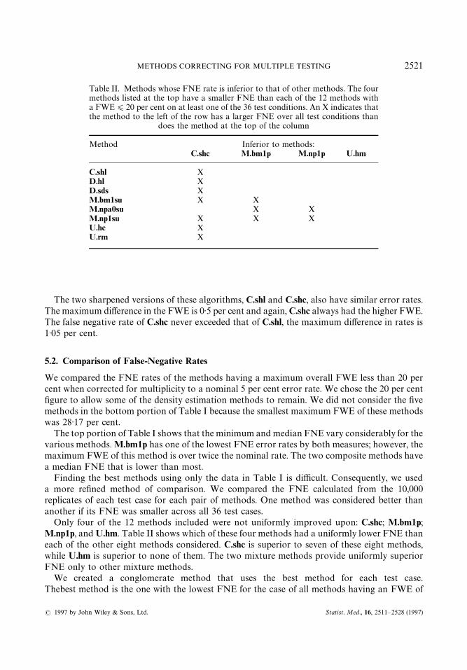
Table II. Methods whose FNE rate is inferior to that of other methods. The fourmethods listed at the top have a smaller FNE than each of the 12 methods witha FWE)20 per cent on at least one of the 36 test conditions. An X indicates thatthe method to the left of the row has a larger FNE over all test conditions than

does the method at the top of the column

Method Inferior to methods:C.shc M.bm1p M.np1p U.hm

C.shl XD.hl XD.sds XM.bm1su X XM.npa0su X XM.np1su X X XU.hc XU.rm X

The two sharpened versions of these algorithms, C.shl and C.shc, also have similar error rates.The maximum difference in the FWE is 0·5 per cent and again, C.shc always had the higher FWE.The false negative rate of C.shc never exceeded that of C.shl, the maximum difference in rates is1·05 per cent.

5.2. Comparison of False-Negative Rates

We compared the FNE rates of the methods having a maximum overall FWE less than 20 percent when corrected for multiplicity to a nominal 5 per cent error rate. We chose the 20 per centfigure to allow some of the density estimation methods to remain. We did not consider the fivemethods in the bottom portion of Table I because the smallest maximum FWE of these methodswas 28·17 per cent.

The top portion of Table I shows that the minimum and median FNE vary considerably for thevarious methods. M.bm1p has one of the lowest FNE error rates by both measures; however, themaximum FWE of this method is over twice the nominal rate. The two composite methods havea median FNE that is lower than most.

Finding the best methods using only the data in Table I is difficult. Consequently, we useda more refined method of comparison. We compared the FNE calculated from the 10,000replicates of each test case for each pair of methods. One method was considered better thananother if its FNE was smaller across all 36 test cases.

Only four of the 12 methods included were not uniformly improved upon: C.shc; M.bm1p;M.np1p, and U.hm. Table II shows which of these four methods had a uniformly lower FNE thaneach of the other eight methods considered. C.shc is superior to seven of these eight methods,while U.hm is superior to none of them. The two mixture methods provide uniformly superiorFNE only to other mixture methods.

We created a conglomerate method that uses the best method for each test case.Thebest method is the one with the lowest FNE for the case of all methods having an FWE of

SIM 693



6 per cent or less for that case. Six methods were chosen as best for one or more of the 36 testcases: C.shc; D.fn; M.bm1p; M.np1p; U.hm, and U.sm. The FNE rate of the conglomerate methodranged from 23 per cent to 91 per cent. Unfortunately, the conglomerate method is unavailablein practice because the number of interesting results, the correlation between the p-values, andthe power of the test for the interesting results are unknown when the p-values arise from actualdata.

Restricting the set of methods available to the conglomerate to the four unsurpassed methods,M.bm1p, U.hm, M.np1p, and C.shc, increases the FNE by up to 22 per cent over that of theunrestricted conglomerate. Each of these four individual methods has a maximum FNE in excessof the original conglomerate by 22 per cent to 36 per cent.

Only one of the methods with an FWE in excess of 20 per cent has an FNE that is uniformlyless than the conglomerate, and this method is U.sm. The maximum excess in FNE over theconglomerate for the other methods is: M.bma0p, 13 per cent; M.bma0su, 15 per cent; D.fn, 7 percent; and M.npa0p, 35 per cent.

6. RECOMMENDATIONS

The results of the previous section clearly show that there is no uniformly best method.Consequently, we recommend a multi-level approach to correlation for multiple hypothesistesting.

Of the methods with an FWE close to the nominal value, C.shc has the smallest FNE rate, andwe recommend it as providing the strongest evidence of reportable results. One could then useU.sm to identify additional results possibly worthy of further investigation, although these couldalso be the consequence of a high FWE. If one desires an intermediate level of identification, oneshould employ one of the density estimation methods, M.bm1p or M.np1p.

7. DISCUSSION

Several of the results surprised the authors. We originally thought that each of the severalmethods would be superior on a few of the test cases. Instead, four of the methods with moderateFWEs were universally unsurpassed. Unfortunately, however, there is not a uniformly bestmethod.

Another surprise was the effect of correlation of the p-values. We originally suspected that itseffect would increase the error rates of the various methods. Instead, the mean error rates changedlittle with increasing correlation, but the variance of the errors greatly increased.

A lesson learned from this investigation is that it is fairly easy to devise new methods to handlemultiple tests of hypotheses. We devised numerous methods during the course of this investiga-tion, but their characteristics were abominable. The only new method included here consists ofthe obvious substitution of non-parametric density estimation for density estimation by thefitting of a mixture of beta densities.

The only guaranteed methods to correct for multiplicity are the Bonferroni method and itsstep-down analogue, D.hl.3,5 Consequently, the use of any other method must be considered asexploratory. All of the methods reported have mathematical support for some cases; unfortunate-ly, this guarantee does not include all realistic cases. Given the lack of mathematical proof of theproperties of a method, testing has a definite place.

SIM 693



8. COMPUTER PROGRAM

A computer program that performs the described computations is available as ANSI Fortran 77source or as Macintosh or DOS executables. The program can be accessed through www using

http://odin.mdacc.tmc.edu/anonftp/

or by anonymous ftp to odin.mdacc.tmc.edu. Ftp users should look at file ./pub/index for thelocation of the program. This program will be posted to statlib.

APPENDIX I: THE METHODS

This appendix contains a detailed description of each examined method for correcting formultiple testing examined here. The reader should consider each description in conjunction withthe exposition of the class of the method in Section 3 of the body of the paper.

I.1. Step-Down Methods

I.1.1. Finner Method (D.fn) (see Finner11,12)

The logical condition, is–small–enough(pj, j), is

p@j"1!(1!p

j) ( j@n))a.

I.1.2. Bonferroni Method (D.hl) (see Holm13)

The logical condition, is–small– (pj, j ), is

p@j"(n!j#1)p

j)a.

I.1.3. S[ ida& k Method (D.sds) (see Westfall and Young3)


p@j"(1!p

j)n~j`1)a.

I.2. Step-Up Methods

I.2.1. Hochberg Method (U.hc) (see Hochberg and Benjamini14)


p@j"(n!j#1)p

j)a.

I.2.2. Hommel Method (U.hm) (see Hommel15)

Hochberg and Benjamini14 discuss the same method and Falk16 gives an interesting extention.The logical condition, is–small– (p

j, j ), is

p@j)a

SIM 693



where

p@j"

pjj

nn+k/1

1

k.

I.2.3. Simes Method (U.sm) (see Simes17)


p@j"

pjj

n)a.

I.2.4. Rom Method (U.rm) (see Rom18)

Define iteratively a list of numbers, c1,2 , c

nby

c1"a.

For i"22n

ci"

i~1+k/1

ck1!

i~2+k/1Ak

iBci~1k`1i

.


p@j)c

j.

I.2.5. Mixture of Beta Distributions

Parker and Rothenberg19 suggest fitting a mixture of beta densities to the observed distributionof p’s by maximum likelihood. The mixture density has the following form:

d (x)"a0b (1, 1) (x)#

K+i/1

aib (r

i, s

i) (x)

where b (r, s) (x) is the incomplete beta density with parameters r and s and the aiare constrained

so that + ai"1. The first component of the mixture is the uniform density, so a

0estimates the

proportion of uninteresting results. In Appendix III we sketch our implementation of this fit.The correction for multiplicity methods related to this fit are M.bma0p, M.bm1p, M.bma0su

and M.bm1su.

I.2.6. Non-parametric Density Estimation

First, one uses the graphic method to estimate m0, the number of uninteresting results. For all but

the m0largest p-values, one makes a pointwise non-parametric density estimate at p not using any

of the m0

points initially deemed uninteresting.To estimate the density of p-values at some p

j, one fits a running weighted local quadratic

model to the cumulative distribution of p-values centred around this point and estimates thedensity by the derivative of this model. Details appear in Appendix IV.

We term the corrections for multiplicity methods derived from this estimate as M.npa0p,M.np1p, M.npa0su and M.np1su.

SIM 693



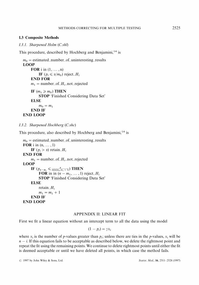
I.3 Composite Methods

I.3.1. Sharpened Holm (C.shl)

This procedure, described by Hochberg and Benjamini,14 is

m0"estimated—number—of—uninteresting—results

LOOPFOR i in (1,2 , n)

IF (pi)a/m

0) reject—Hi

END FORm

1"number—of—Hi—

not—rejected

IF (m1*m

0) THEN

STOP ‘Finished Considering Data Set’ELSE

m0"m

1END IF

END LOOP

I.3.2. Sharpened Hochberg (C.shc)

This procedure, also described by Hochberg and Benjamini,14 is

m0"estimated—number—of—uninteresting—results

FOR i in (n,2 , 1)IF (p

i'a) retain—Hi

END FORm

1"number—of—Hi—

not—rejectedLOOP

IF (pn~m1

) amin(m0, m

1#1) ) THEN

FOR in in (n!m1,2 , 1) reject—Hi

STOP ‘Finished Considering Data Set’ELSE

retain—Him

1"m

1#1

END IFEND LOOP

APPENDIX II: LINEAR FIT

First we fit a linear equation without an intercept term to all the data using the model

(1!pi)"cx

i

where xiis the number of p-values greater than p

i; unless there are ties in the p-values, x

iwill be

n!i. If this equation fails to be acceptable as described below, we delete the rightmost point andrepeat the fit using the remaining points. We continue to delete rightmost points until either the fitis deemed acceptable or until we have deleted all points, in which case the method fails.

SIM 693



We examine the rightmost p-value to determine the acceptability of a fit. If the observed valuelies below the regression line, the regression is acceptable. If the observed value is above the line,we assess the significance of the difference between the observed and predicted value using theusual linear theory that assumes independent normal errors. The residual divided by its standarddeviation yields a t-statistic form which we obtain a p-value. If this p-value is greater than somepredetermined value, we accept the regression. The range of cut-offs for this p-value appears to be0·01 to 0·5. Outside this range, the method is either too conservative or too liberal. We use thevalue 0·05 in the tests reported here.

APPENDIX III: MIXTURE OF BETA DISTRIBUTIONS

There are several user-selectable options in our implementation. One is whether to use the generalminimization code written by David Gay20 or the EM algorithm described by Titteringtonet al.21 to perform the maximum likelihood estimation. The code by Gay is the default and is usedin the tests reported here.

Our computer implementation successively adds beta densities to the mixture model. At eachiteration, we determine starting values for the fit as follows: we identify p-values with probabilityless than 0·05 under the previous model. We fit a beta distribution to these p-values by matchingmean and variance. The initial estimate of a

Kis the proportion of points identified; we multiply

the aifrom the previous model by a constant so that the sum of the as is 1.

There are several criteria provided for choosing K, the number of components in the mixture.The strategy used in the tests reported here is to continue to increase K until a

Kis less than 0·05,

and then to use the previous model. Another available criterion stops when the per cent increasein the log-likelihood is less than a user specified value. A third criterion uses the p-value obtainedfrom the Cramer—von Mises goodnes-of-fit statistic by bootstrapping with use of the previousmodel. A final option prints the information obtained from the various fits and allows the user toselect K. The program, of necessity, stops when fewer than three points have a probability of lessthan 0·05 under the previous model.

APPENDIX IV: NON-PARAMETRIC DENSITY ESTIMATION

We estimate the density of p-values at pjfor values of j estimated by the linear fit as interesting;

points used in the fits are also taken only from this set. We fit a running weighted local quadraticmodel to the negative of the cumulative empirical distribution of p-values centred around each p

j.

Specifically, for each j, we fit a model to obtain a, b and c to minimize

n+i/1

w ( j, i) Gi

n!(a#bp

i#cp2

i)H

2

where

w( j, i )"G1!Ain!j

nh BH

2

for D in!j

nD)h and 0 elsewhere. h is the bandwidth of the weighting function and is chosen by

cross-validation. In cross-validation, for fixed h, we estimate the value of each pi

from theweighted running quadratic equation fit without the data point at p

i. Then we calculate the sum

SIM 693



of squares of deviations of the fit from the observed pi, and choose the value of h that minimizes

this sum of squares.We take the density at p

jas the negative of the derivative of the local quadratic fit to j, that is

!(b#2cpj).

We require a quadratic fit because of edge effects in the estimated density when we employa linear fit.

Fewer points may be found interesting than are required reasonably to fit a running quadratic.Hence, if there are five or fewer such points, we fit a straight line, to yield a constant density. Ifthere are six to ten such points, we fit a single quadratic to all these points.

ACKNOWLEDGEMENTS

This work was supported by grant CA16672 from the National Cancer Institute, by a cooperativestudy agreement with IBM, and by the personal generosity of Larry and Pat McNeil. The authorsare extremely grateful to Peter Westfall of Texas Tech University for his comments on an earlyversion of this work. The authors also thank two anonymous referees whose efforts contributed tomaking this a better work.

REFERENCES

1. Miller, R. G. Simultaneous Statistical Inference, Springer-Verlag, New York, 1981.2. Hochberg, Y. and Tamhane, A. Multiple Comparison Procedures, Wiley, New York, 1987.3 Westfall, P. H. and Young, S. S. Resampling-Based Multiple ¹esting: Examples and Methods for p-value

Adjustment, Wiley, New York, 1993.4. Proschan, M. A. and Follman, D. A. ‘Multiple comparisons with control in a single experiment versus

separate experiments: why do we feel differently?’, American Statistician, 49, 144—149 (1995).5. Aickin, M. and Gensler, H. ‘Adjusting for multiple testing when reporting research results: The

Bonferroni vs Holm Methods’, American Journal of Public Health, 86, 726—728 (1996).6. Benjamini, Y. and Hochberg, Y. ‘Controlling the false discovery rate: a practical and powerful approach

to multiple testing’, Journal of the Royal Statistical Society, Series B, 57, 289—300 (1995).7. Ahrens, J. H. and Dieter, U. ‘Extensions of Forsythe’s method for random sampling from the normal

distribution’, Mathematics of Computing, 27, 927—937 (1973).8. S[ idak, Z. ‘Rectangular confidence regions for the means of multivariate normal distributions’, Journal of

the American Statistical Association, 62, 626—633 (1967).9. S[ idak, Z. ‘On probabilities of rectangles in multivariate Student distributions: their dependence on

correlations’, Annals of Mathematical Statistics, 42, 169—175 (1971).10. Schweder, T. and Spjøtvoll, E. ‘Plots of P-values to evaluate many tests simultaneously’, Biometrika, 69,

493—502 (1982).11. Finner, H. ‘Some new inequalities for the range distribution with application to the determination of

optimum significance levels of multiple range tests’, Journal of the American Statistical Association, 85,191—194 (1990).

12. Finner, H. ‘On a monotonicity problem in step-down multiple test procedures’, Journal of the AmericanStatistical Association, 88, 920—923 (1993).

13. Holm, S. ‘A simple sequentially rejective multiple test procedure’, Scandinavian Journal of Statistics, 6,65—70 (1979).

14. Hochberg, Y. and Benjamini, Y. ‘More powerful procedures for multiple significance testing’, Statisticsin Medicine, 9, 811—818 (1990).

15. Hommel, G. ‘A stagewise rejective multiple test procedure based on a modified Bonferroni test’,Biometrika, 75, 383—386 (1988).

16. Falk, R. W. ‘Hommel’s Bonferroni-type inequality for unequally spaced levels’, Biometrika, 76, 190—191(1989).

SIM 693



17. Simes, R. J. ‘An improved Bonferroni procedure for multiple tests of significance’, Biometrika, 73,751—754 (1986).

18. Rom, Dror M. ‘A sequentially rejective test procedure based on a modified Bonferroni inequality’,Biometrika, 77, 663—665 (1990).

19. Parker, R. A. and Rothenberg, R. B. ‘Identifying important results from multiple statistical tests’,Statistics in Medicine, 7, 1031—1043 (1988).

20. Gay, D. M. ‘Algorithm 611. Subroutines for unconstrained minimization using a model/trust-regionapproach’, ACM ¹ransactions on Mathematical Software, 9, 503—524 (1983).

21. Titterington, D. M., Smith, A. F. M. and Makov, U. E. Statistical Analysis of Finite Mixture Distribu-tions, Wiley, New York, 1985.

.

SIM 693



methods correcting for multiple testing: operating characteristics

Documents