methodology article open access functional mapping of ... · multiple environmental signals through...

METHODOLOGY ARTICLE Open Access

Functional mapping of reaction norms tomultiple environmental signals throughnonparametric covariance estimationJohn S Yap1, Yao Li2, Kiranmoy Das3, Jiahan Li3, Rongling Wu4,3*

Abstract

Background: The identification of genes or quantitative trait loci that are expressed in response to differentenvironmental factors such as temperature and light, through functional mapping, critically relies on precisemodeling of the covariance structure. Previous work used separable parametric covariance structures, such as aKronecker product of autoregressive one [AR(1)] matrices, that do not account for interaction effects of differentenvironmental factors.

Results: We implement a more robust nonparametric covariance estimator to model these interactions within theframework of functional mapping of reaction norms to two signals. Our results from Monte Carlo simulations showthat this estimator can be useful in modeling interactions that exist between two environmental signals. Theinteractions are simulated using nonseparable covariance models with spatio-temporal structural forms that mimicinteraction effects.

Conclusions: The nonparametric covariance estimator has an advantage over separable parametric covarianceestimators in the detection of QTL location, thus extending the breadth of use of functional mapping in practicalsettings.

BackgroundThe phenotype of a quantitative trait exhibits plasticityif the trait differs in phenotypes with changing environ-ment [1-7]. Such environment-dependent changes, alsocalled reaction norms, are ubiquitous in biology. Forexample, thermal reaction norms show how perfor-mance, such as caterpillar growth rate [8] or growthrate and body size in ectotherms [9], varies continuouslywith temperature [10]. Another example is the floweringtime of Arabidopsis thaliana with respect to changinglight intensity [11]. However, QTL mapping of reactionnorms is difficult to model because of the inherent com-plexity in the interplay of a multitude of factorsinvolved. An added difficulty is in their being “infinite-dimensional” as they require an infinite number of mea-surements to be completely described [12]. Wu et al.[13] proposed a functional mapping-based model which

addresses the latter difficulty by using a biologically rele-vant mathematical function to model reaction norms.The authors considered a parametric model of photo-synthetic rate as a function of light irradiance and tem-perature and studied the genetic mechanism of suchprocess. They showed through simulations that in abackcross population with one or two-QTLs, theirmethod accurately and precisely estimated the QTLlocation(s) and the parameters of the mean model forphotosynthesis rate. For a backcross population withone QTL, the mean model consists of two surfaces thatdescribe the photosynthetic rate of two genotypes. How-ever, in their model, they assumed the covariance matrixto be a Kronecker product of two AR(1) structures, eachmodeling a reaction norm due to one environmentalfactor. This type of covariance model is said to be separ-able. Although computationally efficient because of theminimal number of parameters to be estimated, thismodel only captures separate reaction norm effects butfails to incorporate interactions. A more generalapproach is therefore needed.

* Correspondence: [email protected] for Computational Biology, Beijing Forestry University, Beijing100083, PR ChinaFull list of author information is available at the end of the article

Yap et al. BMC Plant Biology 2011, 11:23http://www.biomedcentral.com/1471-2229/11/23

© 2011 Yap et al; licensee BioMed Central Ltd. This is an Open Access article distributed under the terms of the Creative CommonsAttribution License (http://creativecommons.org/licenses/by/2.0), which permits unrestricted use, distribution, and reproduction inany medium, provided the original work is properly cited.

mailto:[email protected]

http://creativecommons.org/licenses/by/2.0

In the context of longitudinal data, Yap et al. [14] pro-posed a nonparametric covariance estimator in func-tional mapping. It was nonparametric in the sense thatthe covariance matrix has an unconstrained set of para-meters to be estimated and not the usual distribution-free sense in nonparametric statistics. This estimatorcan be obtained by employing a modified Choleskydecomposition of the covariance matrix which yieldscomponent matrices whose elements can be interpretedand modeled as terms in a regression [15]. A penalizedlikelihood procedure is used to solve the regression witheither an L1 or L2 penalty [16]. Penalized likelihood inregression is a technique used to obtain minimum meansquared error (MSE) of estimated regression coefficientsby balancing bias and variance. L1 or L2 penalties, whichare functions of the regression covariates, are includedin a regression model in order to shrink coefficientstowards estimates with minimum MSE. In the case ofthe L1 penalty, some of the coefficients are actuallyshrunk to zero. Thus, with the L1 penalty, a more parsi-monious regression model is obtained. The use of pena-lized likelihood with L1 or L2 penalties is particularlyuseful when there is multi-collinearity among the cov-ariates in the regression i.e. when there are near lineardependencies or high correlations among the regressorsor predictor variables. An iterative procedure is imple-mented by using the ECM algorithm [17] to obtain thefinal estimator. Through Monte Carlo simulations, thisnonparametric estimator is found to provide more accu-rate and precise mean parameters and QTL locationestimates than the parametric AR(1) form for the covar-iance model, especially when the underlying covariancestructure of the data is significantly different from theassumed model.The question of how to incorporate interaction effects

in a model with multiple factors has not, to our knowl-edge, been thoroughly explored in the biology literature,especially in the context of genetic mapping that incor-porates interactions of function-valued traits. The spa-tio-temporal literature, however, has a wealth ofpublications that developed more general models suchas nonseparable covariance structures which are used tomodel the underlying interactions of random processesin the space and time domains (see [18,19]). A nonse-parable covariance cannot be expressed as a Kroneckerproduct of two matrices like separable structures can.The random processes being modeled may be the con-centration of pollutants in the atmosphere, groundwatercontaminants, wind speed, or even disposable householdincomes. The main significance of the covariance in thiscontext is in providing a better characterization of therandom process to obtain optimal kriging or predictionof unobserved portions of it. It therefore seems naturalto consider the utilization of nonseparable structures in

the simulation and modeling of reaction norms thatreact to two environmental factors. More concretely, weconsider the photosynthetic rate as a random process,and the irradiance and temperature as the spatial (onedimension) and temporal domains, respectively.The remaining part of this paper is organized as follows:

We first describe the functional mapping model proposedby Wu et al. [13] for reaction norms. Then, we formulateseparable and nonseparable models used in spatio-temporal analyses and present a simulation study usingsome nonseparable structures. Lastly, the new model andits implications for genetic mapping are discussed. Fromhereon, the terms covariance matrix, covariance structureor covariance function are used interchangeably.

Functional Mapping of Reaction NormsReaction Norms: An ExampleWolf [20] described a reaction norm as a surface land-scape determined by genetic and environmental factors.The surface is characterized by a phenotypic trait as afunction of different environmental factors such as tem-perature, light intensity, humidity, etc., and correspondsto a specific genetic effect such as additive, dominant orepistatic [21]. At least in three dimensions, the featuresof the surface such as “slope”, “curvature”, “peak valley”,and “ridge”, can be described graphically to help visua-lize and elucidate how the underlying factors affect thephenotype.An example of reaction norms that illustrate a surface

landscape is photosynthesis [13], the process by whichlight energy is converted to chemical energy by plantsand other living organisms. It is an important yet com-plex process because it involves several factors such asthe age of a leaf (where photosynthesis takes place inmost plants), the concentration of carbon dioxide in theenvironment, temperature, light irradiance, availablenutrients and water in the soil. A mathematical expres-sion for the rate of single-leaf photosynthesis, P, withoutphotorespiration [22] is

PI P

b IP

m

m

= +

−−

2

4

2

2(1)

where b = (aI + Pm, θ Î (0,1) is a dimensionless para-meter, a is the photochemical efficiency, I is the irradi-ance, and Pm is the asymptotic photosynthetic rate at asaturating irradiance. Pm is a linear function of the tem-perature, T

PP P T T T

T Tm

m=≥

<

⎧⎨⎪

⎩⎪

( ) ( ) *

,*

20

0(2)


of 13

where P TT T

T( )

*

*= −−20

, Pm(20) is the value of Pm at

the reference temperature of 20°C and T* is the tem-perature at which photosynthesis stops. T* is chosenover a range of temperatures, such as 5°C-25°C, to pro-vide a good fit to observed data.Wu et al. [13] studied the reaction norm of photosyn-

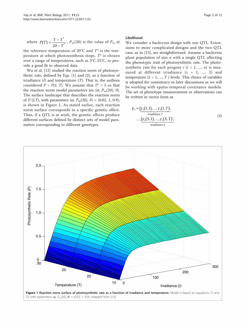
thetic rate, defined by Eqs. (1) and (2), as a function ofirradiance (I) and temperature (T). That is, the authorsconsidered P = P(I, T). We assume that T* = 5 so thatthe reaction norm model parameters are (a, Pm(20), θ).The surface landscape that describes the reaction normof P (I,T), with parameters (a, Pm(20), θ) = (0.02, 1, 0.9),is shown in Figure 1. As stated earlier, each reactionnorm surface corresponds to a specific genetic effect.Thus, if a QTL is at work, the genetic effects producedifferent surfaces defined by distinct sets of model para-meters corresponding to different genotypes.

LikelihoodWe consider a backcross design with one QTL. Exten-sions to more complicated designs and the two-QTLcase, as in [13], are straightforward. Assume a backcrossplant population of size n with a single QTL affectingthe phenotypic trait of photosynthetic rate. The photo-synthetic rate for each progeny i (i = 1, ..., n) is mea-sured at different irradiance (s = 1, ..., S) andtemperature (t = 1, ..., T ) levels. This choice of variablesis adopted for consistency in later discussions as we willbe working with spatio-temporal covariance models.The set of phenotype measurements or observations canbe written in vector form as

y i i i

i

y y T

y S

= [ ( , ),..., ( , ),

... ,[ ( , ),

1 1 1

1irradiance 1

...., ( , ) ,y S Ti ’

irradiance S

(3)

0

100

200

300

15

20

25

300

0.5

1.0

1.5

2.0

Irradiance (I)Temperature (T)

Pho

tosy

nthe

tic R

ate

(P)

Figure 1 Reaction norm surface of photosynthetic rate as a function of irradiance and temperature. Model is based on equations (1) and(2) with parameters (a, Pm(20), θ) = (0.02, 1, 0.9). Adapted from [13].


of 13

The progeny are genotyped for molecular markers toconstruct a genetic linkage map for the segregating QTLin the population. This means that the genotypes of themarkers are observed and will be used, along with thephenotype measurements, to predict the QTL. With abackcross design, the QTL has two possible genotypes(as do the markers) which shall be indexed by k = 1, 2.The likelihood function based on the phenotype andmarker data can be formulated as

L p fk i

k

k i

i

n

( ) ( | )|Ω Ω=⎡

⎣⎢⎢

⎤

⎦⎥⎥==

∑∏1

2

1

y (4)

where pk|i is the conditional probability of a QTL gen-otype given the genotype of a marker interval for pro-geny i. We assume a multivariate normal density for thephenotype vector yi with genotype-specific means

k k k

k

T

S

= [ ( , ),..., ( , ),

... ,[ ( , ),

1 1 1

1irradiance 1

...., ( , )’,k S Tirradiance S

(5)

and covariance matrix Σ = cov(yi).

Mean and Covariance ModelsThe mean vector for photosynthetic rate in (5) can bemodeled using equations (1) and (2) as

kk mk

k

k k k mk

k

s ts P

b sP

( , ) = +

−−

2

4

2

2 (6)

Where bk = aks + Pmk,

P tP P t t T

t Tmk

mk( )

( ) ( ) **

=≥

<

⎧⎨⎪

⎩⎪

20

0(7)

P tt T

T( )

*

*= −−20

and k = 1, 2.

Wu et al. [13] used a separable structure (Mitchellet al., 2005) for the ST × ST covariance matrix Σ as

Σ Σ ΣAR( )1 1 2= ⊗ (8)

where Σ1 and Σ2 are the (S×S) and (T×T) covariancematrices among different irradiance and temperaturelevels, respectively, and ⊗ is the Kronecker productoperator. Note that Σ1 and Σ2 are unique only up tomultiples of a constant because for some |c| > 0, cΣ1 ⊗(1/c)Σ2 = Σ1 ⊗ Σ2. Each of Σ1 and Σ2 is modeled using

an AR(1) structure with a common error variance, s2,and correlation parameters rk (k = 1, 2):

Σ k

k kS

k kS

kS

kS

=

⎡

⎣

⎢⎢⎢⎢⎢

⎤

⎦

⎥⎥⎥⎥⎥

−

−

− −

2

1

2

1 2

1

1

1

(9)

Separable covariance structures, however, cannotmodel interaction effects of each reaction norm to tem-perature and irradiance. Thus, there is a need for amore general model for this purpose.Yap et al. [14] proposed to use a data-driven nonpara-

metric covariance estimator in functional mapping. Theauthors showed that using such estimator provides bet-ter estimates for QTL location and mean model para-meters when compared to AR(1). Huang et al. [16]showed that the nonparametric estimator works well forlarge matrices. Functional mapping of reaction normswhen there are two environmental signals necessitatesthe use of large covariance matrices that result fromKronecker products of smaller matrices. Here, we areinterested in determining whether the nonparametriccovariance estimator of Yap et al. [14] will still workwell in this reaction norm setting.It should be noted that unlike parametric models, e.g.

AR(1), there are no parameters being estimated in thenonparametric covariance estimator. The entries of thematrix are determined based on the data. This is differ-ent from a model-dependent covariance matrix modelwith one parameter for each of its elements. Due toover-parametrization, such a model may not lead toconvergence to yield reliable results.Note that with (6)-(9), Ω = Ω1 ∪ Ω2 in (4), where Ω1

= {a1, Pm1(20), θ1, s2, r1} and Ω1 = {a2, Pm2(20), θ2, s2,r2}. These model parameters may be estimated usingthe ECM algorithm [17], but closed form solutions atthe CM-step are be very complicated. A more efficientmethod is to use the Nelder-Mead simplex algorithm[23] which can be easily implemented using softwaressuch as Matlab.

Hypothesis TestsThe features of the surface landscape are importantbecause they can be used as a basis in formulatinghypothesis tests. Let H0 and H1 denote the null andalternative hypotheses, respectively. Then the existenceof a QTL that determines the reaction norm curves canbe formulated as

H P Pm m0 1 2 1 1 220 20: , ( ) ( ), , = = =

versus


of 13

H1 : at least one of the equalities

above does not hold

This means that if the reaction norm curves are dis-tinct (in terms of their respective estimated parameters),then a QTL possibly exists. The estimated location ofthe QTL is at the point at which the log-likelihood ratioobtained using the null and alternative hypotheses ismaximal. Of course a slight difference in parameter esti-mates does not automatically mean a QTL exists. Thesignificance of the results can be determined by permu-tation tests [24] which involves a repeated application ofthe functional mapping model on the data where thephenotype and marker associations are broken to simu-late the null hypothesis of no QTL. A significance levelis then obtained based on the maximal log-likelihoodratio at each application to infer the presence or absenceof a QTL (see ref. [25] for more details). A proceduredescribed in ref. [26] can be used to test the additiveeffects of a QTL. Other hypotheses can be formulatedand tested such as the genetic control of the reactionnorm to each environmental factor, interaction effectsbetween environmental factors on the phenotype, andthe marginal slope of the reaction norm with respect toeach environmental factor or the gradient of the reac-tion norm itself. The reader is referred to Wu et al. [13]for more details.

Spatio-Temporal CovariancesWe investigate the use of parametric and nonseparablespatio-temporal covariance structures in functional map-ping of photosynthetic rate as a reaction norm to theenvironmental factors irradiance and temperature. Asstated earlier, the main idea is to model irradiance as aone-dimensional spatial variable and temperature as atemporal variable. The choice of which environmentalsignal is modeled as temporal or spatial is arbitrary. Formore about spatio-temporal modeling, we refer thereader to [27,19].

Basic Ideas, Notation, and AssumptionsWe consider a real-valued spatio-temporal random pro-cess given by

Y s t s t dd( , ), ( , ) ,∈ × ∈ + (10)

where observations are collected at coordinates

( , ),( , ),...,( , )s t s t s tN N1 1 2 2

to characterize unobserved portions of the process.This collection of coordinates are not necessarilyordered fixed levels of each trait. We will only be

concerned with the case d = 1. Aside from those men-tioned earlier, Y may also represent ozone levels, diseaseincidence, ocean current patterns or water temperatures.In our setting, Y represents photosynthetic rate.If var (Y(s, t)) < ∞ for all (s, t) Î ℛ × ℛ, then the

covariance, cov (Y(s, t), Y(s + u, t + v)), where u and vare spatial and temporal lags, respectively, exists. Weassume that the covariance is stationary in space andtime so that for some function C,

cov ( ( , ), ( , )) ( , ).Y s t Y s u t v C u v+ + = (11)

This means that the covariance function C dependsonly on the lags and not on the values of the coordi-nates themselves. Stationarity is often assumed to allowestimation of the covariance function from the data[18]. We also assume that the covariance function is iso-tropic which means that it depends only on the absolutelags and not in the direction or orientation of the coor-dinates to each other. The covariances considered inthis paper are positive (semi-) definite as they satisfy thefollowing condition: for any (s1, t1), ..., (sk , tk) Î ℛ ×ℛ, any real coefficients a1, ..., ak, and any positive inte-ger k,

a a C s s t ti

j

k

i

k

j i j i j

==∑∑ − − ≥

11

0( , ) (12)

Note that C(u, 0) and C(0, v) correspond to purelyspatial and purely temporal covariance functions,respectively.In spatio-temporal analysis, the ultimate goal is opti-

mal prediction (or kriging) of an un-observed part ofthe random process Y(s, t) using an appropriate covar-iance function model. We utilize a covariance model tocalculate the mixture likelihood associated with func-tional mapping.

Separable and Nonseparable Covariance StructuresSeparable Covariance StructuresA covariance function C(u, v|θ) of a spatio-temporalprocess is separable if it can be expressed as

C u v C u C v( , | ) ( | ) ( | ) = 1 1 2 2 (13)

where C1(u|θ1) and C2(v|θ2) are purely spatial andpurely temporal covariance functions, respectively, and θ= (θ1, θ2)’. This representation implies that the observedjoint process can be seen as a product of two indepen-dent spatial and temporal processes.A more general definition for separability is as a Kro-

necker product (equation (8)). From equation (8), it can be

shown that Σ Σ ΣAR( )11

11

21− − −= ⊗ and | | | | | |( )Σ Σ ΣAR

d d1 1 2

2 1= ,


of 13

where |·| denotes the determinant of a matrix; d1 and d2are the dimensions of Σ1 and Σ2, respectively. This illus-trates the computational advantage of using separablemodels in likelihood estimation where the inverse anddeterminant of the covariance matrix are calculated. For alarge covariance matrix of dimension UV, its inverse canbe calculated from the inverses of its Kronecker compo-nent matrices, Σ1 and Σ2, with dimensions U and V,respectively. Thus, the inversion of a 100 × 100 matrix, forexample, may only require the inversion of two 10 × 10matrices. A similar argument can be used for the determi-nant. ΣAR(1) can be put in the form (13) as

C u v u v

u v

( , | , , )

,

21 2

21

22

41 2

=

=

. (14)

where u = 1, ..., U , v = 1, ..., V. Note that this modelassumes equidistant or regularly spaced coordinates.Thus, two consecutive or closest neighbor coordinateswill have the same correlation structure as another evenif their respective distances are different. A more appro-priate model might be

C u v a b u a v b( , | , , , , ) / / 21 2

41 2= (15)

where a and b are scale parameters. In this model, thescale parameters correct for the uneven distancesbetween coordinates.Nonseparable Covariance StructuresHere, we present some nonseparable covariance modelsthat were derived in two different ways. The details ofthe derivation are omitted as they are rather compli-cated and lengthy.The following nonseparable covariance models were

derived by Cressie and Huang [18] using the Fouriertransform of the spectral density and by utilizing Boch-ner’s Theorem [28]:

C u va v

b u

a v

( , )( )

exp ,

=+

× −+

⎛

⎝⎜⎜

⎞

⎠⎟⎟

2

2 2

2 2

2 2

1

1

(16)

C u va v

a v b u( , )

( | | )

( | | ) | |= +

+ + 2

2 2 2

1

1(17)

C u v a v b u

c v u

( , ) exp( | | | | )

exp( | || | ),

= − −

× −

2 2 2

2(18)

where a, b ≥ 0 are scaling parameters of time andspace, respectively; c ≥ 0 is an interaction parameter oftime and space, and s2 = C(0, 0) ≥ 0. Note that when c= 0, (18) reduces to a separable model.

Gneiting [27] developed an approach that can producenonseparable covariance models without relying onFourier transform pairs. One such model is

C u va v

b u

a v

( , )( | | )

exp| |

( | | ),

=+

× −+

⎛

⎝⎜⎜

⎞

⎠⎟⎟

2

2

2

2

1

1

(19)

with (u, v) Î ℛ × ℛ and where a, b > 0 are scalingparameters of space and time, respectively; a, b Î (0, 1]are smoothness parameters of space and time, respec-tively; g 0[1]; τ ≥ 1/2; and s2 ≥ 0. g is a space-time inter-action parameter which implies a separable structurewhen 0 and a nonseparable structure otherwise. Increas-ing values of g indicates strengthening spatio-temporalinteraction.

Computer SimulationWe investigated the performances of the following non-separable covariances structures that were presented inthe preceding section

C u va v

b u

a v

1

2

2 2

2 2

2 2

1

1

( , )( )

exp ,

=+

× −+

⎛

⎝⎜⎜

⎞

⎠⎟⎟

(20)

C u va v

a v b u2

2

2 2 2

1

1( , )

( | | )

( | | ) | |,= +

+ +

(21)

C u va v

b u

a v

3

2

2

1

1

( , )( | | )

exp| |

( | | ),/

=+

× −+

⎛

⎝⎜⎜

⎞

⎠⎟⎟

(22)

where a, b ≥ 0; g Î 0[1] and s2 > 0. C1 and C2 corre-spond to (16) and (17), respectively, and C3 is a specialcase of (19) with a = 1/2, b = 1/2 and τ = 1.We generated photosynthetic rate data using these

nonseparable covariances to simulate interaction effectsbetween the two environmental signals in functionalmapping of a reaction norm. The generated data wasanalyzed using the nonparametric estimator ΣNP pro-posed by Yap et al. [14] using an L2 penalty, and ΣAR(1)(equation (8)). Note that the underlying covariancestructures were very different from the assumed model,ΣAR(1) , and we therefore expected to get biased esti-mates. The issue we wanted to address was the extent


of 13

to which the bias cannot be ignored and an alternativeestimator such as ΣNP may be more appropriate.Covariance fit was assessed using entropy (LE) and

quadratic (LQ) losses:

L mE( , ) ( ) logΣ Σ Σ Σ Σ Σ= − −− −tr 1 1

and

L IQ( , ) ( )Σ Σ Σ Σ= −−tr 1 2

where Σ̂ is the estimate of the true underlying covar-

iance Σ [14,16,29-31]. Each loss function is 0 when

Σ̂ Σ= and large values suggest significant bias.

Using a backcross design for the QTL mapping popu-lation, we randomly generated 6 markers equally spacedon a chromosome 100 cM long. One QTL was simu-lated between the fourth and fifth markers, 12 cM fromthe fourth marker (or 72 cM from the leftmost markerof the chromosome). The QTL had two possible geno-types which determined two distinct mean photosyn-thetic rate reaction norm surfaces defined by equations(1) and (2) (see also Figure 1). The surface parametersfor each genotype were (a1, Pm1(20), θ1) = (0.02, 2, 0.9)and (a2, Pm2(20), θ2) = (0.01, 1.5, 0.9). Phenotype obser-vations were obtained by sampling from a multivariatenormal distribution with mean surface based on irradi-ance and temperature levels of {0, 50, 100, 200, 300}and {15, 20, 25, 30}, respectively, and covariance matrixCl(u, v), l = 1, 2, 3 with a = 0.50, b = 0.01 for C1, a =1.00, b = 0.01 for C2, a = 1.00, b = 0.01, c = 0.60 for C3

and s2 = 1.00 for all three covariances.Figure 2 shows the reaction norm surfaces of photo-

synthetic rate as functions of irradiance and temperaturethat were used in the simulation. Within the considereddomain of values for irradiance and temperature, onesurface lies above the other. These surfaces differ onlyin terms of the a2 and Pm1(20) parameters.The functional mapping model was applied to the

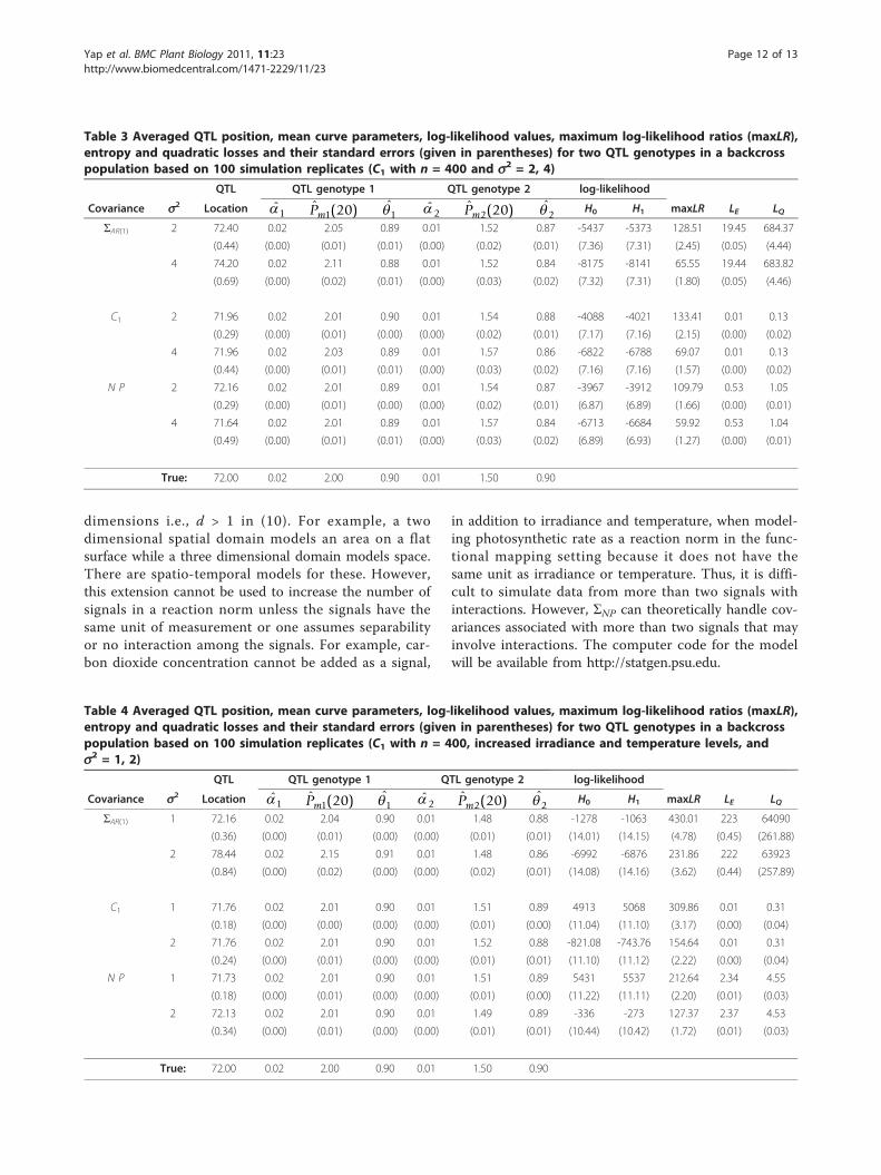
marker and phenotype data with n = 200, 400 samples.The surface defined by equations (1) and (2) was usedas mean model with ΣNP and ΣAR(1) as covariance mod-els to analyze the data generated using Cl(u, v). 100simulation runs were carried out and the averages on allruns of the estimated QTL location, mean parameterestimates, entropy and quadratic losses, including therespective Monte carlo standard errors (SE), wererecorded. Tables 1 and 2 present the results of thesesimulations. The results show that using ΣNP yields rea-sonably accurate and precise parameter estimates. Theresults for ΣAR(1) are similar to ΣNP except that the aver-age losses, given by LE and LQ, are inflated for C1 and

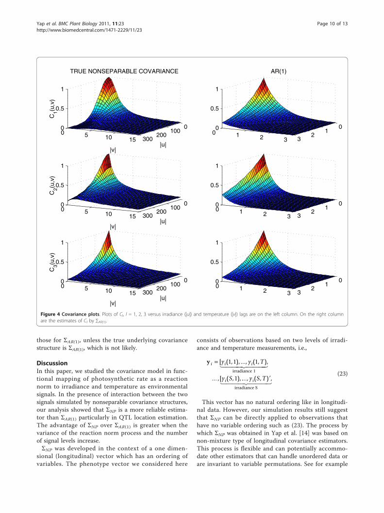
C2. Figure 3 shows box plots of the log-likelihood valuesunder the alternative model. These plots reveal biasedestimates of C1 and C2 by ΣAR(1) and the degrees of biasare consistent with the average losses. The results forthe log-likelihood values under the null model are verysimilar but are not shown. We also provided the covar-iance and corresponding contour plots of Cl(u, v), l = 1,2, 3 and the ΣAR(1) estimates of these in Figure 4 and 5.We only provided plots for Cl(u, v), l = 1, 2, 3 and ΣAR(1) to illustrate the behavior of these parametric models.We did not include plots for the estimated ΣNP becausethere are no parametric estimates for this model and wedid not record all elements of the estimated ΣNP in thesimulation runs.We conducted further simulations using C1 as the

underlying covariance structure of the data with n =400. This was the case where ΣAR(1) performed theworst. We considered two scenarios: increased varianceparameter, s2, or increased irradiance and temperaturelevels (finer grid). That is,

1. s2 = 2, 4 with irradiance and temperature levels of{0, 50, 100, 200, 300} and {15, 20, 25, 30},respectively.2. s2 = 1, 2 with irradiance and temperature levels of{0, 50, 100, 150, 200, 250, 300} and {15, 18, 21, 24,27, 30}, respectively.

We included an analysis of the simulated data usingC1 as the covariance model to ensure the results are notfalse-positives. The results of the simulation are shownin Tables 3 and 4. The tables include columns for thelog-likelihood values under the null (H0) and alternative(H1) hypotheses as well as the maximum of the log-like-lihood ratio (maxLR). MaxLR is used in permutationtests to assess significance of QTL existence (see Section2.3). Under scenarios (1) or (2), i.e. increased varianceparameter s2 or increased irradiance and temperaturelevels, using ΣNP yields significantly more accurate andprecise estimates of the QTL location compared to ΣAR(1): In Table 3, when s2 = 4, the estimates of the trueQTL location of 72 were 71.64 and 74.20 for NP andΣAR(1), respectively; In Table 4, when s2 = 2, the esti-mates were 72.13 and 78.44. Although for ΣAR(1), maxLRappears to be more accurate, the log-likelihood ratiosare still significantly different from the estimates givenby C1. Again, this is reflected in the inflated averagelosses. Note that the maxLR estimates are larger for ΣAR(1) when compared to those for ΣNP. We do not expectthis to be always the case. In other instances, the maxLRestimates for ΣAR(1) may be smaller than those for ΣNP .However, in those instances, we expect the maxLR esti-mates for ΣNP to still be more accurate and precise than


of 13

0 100 200 30010

2030

0

1

2

3

4

0 100 200 300

10

20

300

1

2

3

4

0200

40015 20 25 30

0

1

2

3

4

0100200300

10

20

30

0

1

2

3

4

Figure 2 Reaction norm surfaces of photosynthetic rate as functions of irradiance and temperature. Models are based on equations (1)and (2) with parameters (a1, Pm1(20), θ1) = (0.02, 2, 0.9) and (a2, Pm2(20), θ2) = (0.01, 1.5, 0.9) as used in the simulation.

Table 1 Averaged QTL position, mean curve parameters, entropy and quadratic losses and their standard errors (givenin parentheses) for two QTL genotypes in a backcross population under different sample sizes (n) based on 100simulation replicates (ΣNP)

QTL QTL genotype 1 QTL genotype 2

Covariance n Location ̂1ˆ ( )Pm1 20 ̂1 ̂2

ˆ ( )Pm2 20 ̂2 LE LQ

C1 200 71.68 0.02 2.02 0.90 0.01 1.52 0.88 1.04 2.03

(0.28) (0.00) (0.01) (0.00) (0.00) (0.02) (0.01) (0.01) (0.02)

400 72.16 0.02 2.00 0.90 0.01 1.52 0.88 0.53 1.06

(0.23) (0.00) (0.01) (0.00) (0.00) (0.01) (0.01) (0.00) (0.01)

C2 200 71.88 0.02 2.00 0.90 0.01 1.53 0.88 1.00 1.96

(0.29) (0.00) (0.01) (0.00) (0.00) (0.01) (0.01) (0.01) (0.02)

400 71.92 0.02 2.00 0.90 0.01 1.52 0.89 0.52 1.02

(0.17) (0.00) (0.01) (0.00) (0.00) (0.01) (0.01) (0.00) (0.01)

C3 200 72.12 0.02 2.01 0.89 0.01 1.54 0.87 0.88 1.70

(0.37) (0.00) (0.01) (0.01) (0.00) (0.02) (0.01) (0.01) (0.02)

400 72.08 0.02 2.01 0.90 0.01 1.52 0.89 0.48 0.94

(0.20) (0.00) (0.01) (0.00) (0.00) (0.01) (0.01) (0.00) (0.01)

True: 72.00 0.02 2.00 0.90 0.01 1.50 0.90


of 13

Table 2 Averaged QTL position, mean curve parameters, entropy and quadratic losses and their standard errors (givenin parentheses) for two QTL genotypes in a backcross population under different sample sizes (n) based on 100simulation replicates (ΣAR(1))

QTL QTL genotype 1 QTL genotype 2

Covariance n Location ̂1ˆ ( )Pm1 20 ̂1 ̂2

ˆ ( )Pm2 20 ̂2 LE LQ

C1 200 72.32 0.02 2.03 0.90 0.01 1.53 0.87 19.43 681.78

(0.45) (0.00) (0.01) (0.01) (0.00) (0.02) (0.01) (0.07) (6.16)

400 71.72 0.02 2.03 0.90 0.01 1.51 0.89 19.45 684.11

(0.27) (0.00) (0.01) (0.00) (0.00) (0.01) (0.01) (0.05) (4.40)

C2 200 71.96 0.02 2.01 0.90 0.01 1.55 0.87 4.83 58.60

(0.34) (0.00) (0.01) (0.00) (0.00) (0.02) (0.01) (0.02) (1.01)

400 71.84 0.02 2.01 0.90 0.01 1.52 0.89 4.83 58.61

(0.20) (0.00) (0.01) (0.00) (0.00) (0.01) (0.01) (0.02) (0.77)

C3 200 72.00 0.02 2.01 0.89 0.01 1.54 0.87 0.60 1.51

(0.35) (0.00) (0.01) (0.01) (0.00) (0.02) (0.01) (0.00) (0.10)

400 71.96 0.02 2.01 0.89 0.01 1.52 0.89 0.60 1.43

(0.22) (0.00) (0.01) (0.00) (0.00) (0.01) (0.01) (0.00) (0.08)

True: 72.00 0.02 2.00 0.90 0.01 1.50 0.90

−1500

−1100

−700

−300n=200

log−

likel

ihoo

d, H

1

−3000

−2000

−1000

n=400

log−

likel

ihoo

d, H

1

−1300

−950

−600

log−

likel

ihoo

d, H

1

−2500

−2100

−1700

−1300

log−

likel

ihoo

d, H

1

−1700

−1400

−1100

log−

likel

ihoo

d, H

1

−3300

−2950

−2600

log−

likel

ihoo

d, H

1

NP C1 AR(1) NP C

1

NP C2 NP C

2

NP C3 NP C

3

AR(1)

AR(1) AR(1)

AR(1) AR(1)

Figure 3 Boxplots of the values of the log-likelihood under the alternative model, H1. Significantly biased estimates by ΣAR(1) are apparentfor C1.


of 13

those for ΣAR(1), unless the true underlying covariancestructure is ΣAR(1), which is not likely.

DiscussionIn this paper, we studied the covariance model in func-tional mapping of photosynthetic rate as a reactionnorm to irradiance and temperature as environmentalsignals. In the presence of interaction between the twosignals simulated by nonseparable covariance structures,our analysis showed that ΣNP is a more reliable estima-tor than ΣAR(1) particularly in QTL location estimation.The advantage of ΣNP over ΣAR(1) is greater when thevariance of the reaction norm process and the numberof signal levels increase.ΣNP was developed in the context of a one dimen-

sional (longitudinal) vector which has an ordering ofvariables. The phenotype vector we considered here

consists of observations based on two levels of irradi-ance and temperature measurements, i.e.,

y i i i

i

y y T

y S

= [ ( , ),..., ( , ),

... ,[ ( , ),

1 1 1

1irradiance 1

...., ( , )’,y S Ti

irradiance S

(23)

This vector has no natural ordering like in longitudi-nal data. However, our simulation results still suggestthat ΣNP can be directly applied to observations thathave no variable ordering such as (23). The process bywhich ΣNP was obtained in Yap et al. [14] was based onnon-mixture type of longitudinal covariance estimators.This process is flexible and can potentially accommo-date other estimators that can handle unordered data orare invariant to variable permutations. See for example

0 100

200300

0 5 10 15

0

0.5

1

|u|

TRUE NONSEPARABLE COVARIANCE

|v|

C1(u

,v)

01

23

0 1 2 3

0

0.5

1

AR(1)

0 100

200300

0 5 10 15

0

0.5

1

|u||v|

C2(u

,v)

01

23

0 1 2 3

0

0.5

1

0 100

200300

0 5 10 15

0

0.5

1

|u||v|

C3(u

,v)

01

23

0 1 2 3

0

0.5

1

Figure 4 Covariance plots. Plots of Cl, l = 1, 2, 3 versus irradiance (|u|) and temperature (|v|) lags are on the left column. On the right columnare the estimates of Cl by ∑AR(1).


of 13

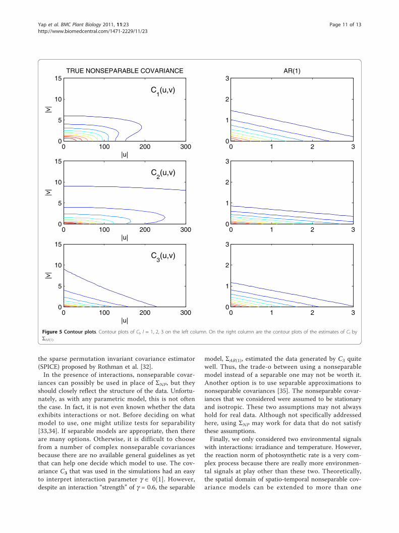
the sparse permutation invariant covariance estimator(SPICE) proposed by Rothman et al. [32].In the presence of interactions, nonseparable covar-

iances can possibly be used in place of ΣNP, but theyshould closely reflect the structure of the data. Unfortu-nately, as with any parametric model, this is not oftenthe case. In fact, it is not even known whether the dataexhibits interactions or not. Before deciding on whatmodel to use, one might utilize tests for separability[33,34]. If separable models are appropriate, then thereare many options. Otherwise, it is difficult to choosefrom a number of complex nonseparable covariancesbecause there are no available general guidelines as yetthat can help one decide which model to use. The cov-ariance C3 that was used in the simulations had an easyto interpret interaction parameter g Î 0[1]. However,despite an interaction “strength” of g = 0.6, the separable

model, ΣAR(1), estimated the data generated by C3 quitewell. Thus, the trade-o between using a nonseparablemodel instead of a separable one may not be worth it.Another option is to use separable approximations tononseparable covariances [35]. The nonseparable covar-iances that we considered were assumed to be stationaryand isotropic. These two assumptions may not alwayshold for real data. Although not specifically addressedhere, using ΣNP may work for data that do not satisfythese assumptions.Finally, we only considered two environmental signals

with interactions: irradiance and temperature. However,the reaction norm of photosynthetic rate is a very com-plex process because there are really more environmen-tal signals at play other than these two. Theoretically,the spatial domain of spatio-temporal nonseparable cov-ariance models can be extended to more than one

0 100 200 3000

5

10

15

|u|

|v|

TRUE NONSEPARABLE COVARIANCE

0 1 2 30

1

2

3AR(1)

0 100 200 3000

5

10

15

|u|

|v|

0 1 2 30

1

2

3

0 100 200 3000

5

10

15

|u|

|v|

0 1 2 30

1

2

3

C1(u,v)

C2(u,v)

C3(u,v)

Figure 5 Contour plots. Contour plots of Cl, l = 1, 2, 3 on the left column. On the right column are the contour plots of the estimates of Cl byΣAR(1).


of 13

dimensions i.e., d > 1 in (10). For example, a twodimensional spatial domain models an area on a flatsurface while a three dimensional domain models space.There are spatio-temporal models for these. However,this extension cannot be used to increase the number ofsignals in a reaction norm unless the signals have thesame unit of measurement or one assumes separabilityor no interaction among the signals. For example, car-bon dioxide concentration cannot be added as a signal,

in addition to irradiance and temperature, when model-ing photosynthetic rate as a reaction norm in the func-tional mapping setting because it does not have thesame unit as irradiance or temperature. Thus, it is diffi-cult to simulate data from more than two signals withinteractions. However, ΣNP can theoretically handle cov-ariances associated with more than two signals that mayinvolve interactions. The computer code for the modelwill be available from http://statgen.psu.edu.

Table 3 Averaged QTL position, mean curve parameters, log-likelihood values, maximum log-likelihood ratios (maxLR),entropy and quadratic losses and their standard errors (given in parentheses) for two QTL genotypes in a backcrosspopulation based on 100 simulation replicates (C1 with n = 400 and s2 = 2, 4)

QTL QTL genotype 1 QTL genotype 2 log-likelihood

Covariance s2 Location ̂1ˆ ( )Pm1 20 ̂1 ̂2

ˆ ( )Pm2 20 ̂2 H0 H1 maxLR LE LQ

ΣAR(1) 2 72.40 0.02 2.05 0.89 0.01 1.52 0.87 -5437 -5373 128.51 19.45 684.37

(0.44) (0.00) (0.01) (0.01) (0.00) (0.02) (0.01) (7.36) (7.31) (2.45) (0.05) (4.44)

4 74.20 0.02 2.11 0.88 0.01 1.52 0.84 -8175 -8141 65.55 19.44 683.82

(0.69) (0.00) (0.02) (0.01) (0.00) (0.03) (0.02) (7.32) (7.31) (1.80) (0.05) (4.46)

C1 2 71.96 0.02 2.01 0.90 0.01 1.54 0.88 -4088 -4021 133.41 0.01 0.13

(0.29) (0.00) (0.01) (0.00) (0.00) (0.02) (0.01) (7.17) (7.16) (2.15) (0.00) (0.02)

4 71.96 0.02 2.03 0.89 0.01 1.57 0.86 -6822 -6788 69.07 0.01 0.13

(0.44) (0.00) (0.01) (0.01) (0.00) (0.03) (0.02) (7.16) (7.16) (1.57) (0.00) (0.02)

N P 2 72.16 0.02 2.01 0.89 0.01 1.54 0.87 -3967 -3912 109.79 0.53 1.05

(0.29) (0.00) (0.01) (0.00) (0.00) (0.02) (0.01) (6.87) (6.89) (1.66) (0.00) (0.01)

4 71.64 0.02 2.01 0.89 0.01 1.57 0.84 -6713 -6684 59.92 0.53 1.04

(0.49) (0.00) (0.01) (0.01) (0.00) (0.03) (0.02) (6.89) (6.93) (1.27) (0.00) (0.01)

True: 72.00 0.02 2.00 0.90 0.01 1.50 0.90

Table 4 Averaged QTL position, mean curve parameters, log-likelihood values, maximum log-likelihood ratios (maxLR),entropy and quadratic losses and their standard errors (given in parentheses) for two QTL genotypes in a backcrosspopulation based on 100 simulation replicates (C1 with n = 400, increased irradiance and temperature levels, ands2 = 1, 2)

QTL QTL genotype 1 QTL genotype 2 log-likelihood

Covariance s2 Location ̂1ˆ ( )Pm1 20 ̂1 ̂2

ˆ ( )Pm2 20 ̂2 H0 H1 maxLR LE LQ

ΣAR(1) 1 72.16 0.02 2.04 0.90 0.01 1.48 0.88 -1278 -1063 430.01 223 64090

(0.36) (0.00) (0.01) (0.00) (0.00) (0.01) (0.01) (14.01) (14.15) (4.78) (0.45) (261.88)

2 78.44 0.02 2.15 0.91 0.01 1.48 0.86 -6992 -6876 231.86 222 63923

(0.84) (0.00) (0.02) (0.00) (0.00) (0.02) (0.01) (14.08) (14.16) (3.62) (0.44) (257.89)

C1 1 71.76 0.02 2.01 0.90 0.01 1.51 0.89 4913 5068 309.86 0.01 0.31

(0.18) (0.00) (0.00) (0.00) (0.00) (0.01) (0.00) (11.04) (11.10) (3.17) (0.00) (0.04)

2 71.76 0.02 2.01 0.90 0.01 1.52 0.88 -821.08 -743.76 154.64 0.01 0.31

(0.24) (0.00) (0.01) (0.00) (0.00) (0.01) (0.01) (11.10) (11.12) (2.22) (0.00) (0.04)

N P 1 71.73 0.02 2.01 0.90 0.01 1.51 0.89 5431 5537 212.64 2.34 4.55

(0.18) (0.00) (0.01) (0.00) (0.00) (0.01) (0.00) (11.22) (11.11) (2.20) (0.01) (0.03)

2 72.13 0.02 2.01 0.90 0.01 1.49 0.89 -336 -273 127.37 2.37 4.53

(0.34) (0.00) (0.01) (0.00) (0.00) (0.01) (0.01) (10.44) (10.42) (1.72) (0.01) (0.03)

True: 72.00 0.02 2.00 0.90 0.01 1.50 0.90


of 13

http://statgen.psu.edu

AcknowledgementsThis work is partially supported by NSF grant IOS-0923975, the ChangjiangScholarship Award and “One-thousand Person Plan” Award at BeijingForestry University.

Author details1Department of Statistics, University of Florida, Gainesville, FL 32611 USA.2Department of Statistics, West Virginia University, Morgantown, WV 26506,USA. 3Center for Statistical Genetics, Pennsylvania State University, Hershey,PA 17033, USA. 4Center for Computational Biology, Beijing ForestryUniversity, Beijing 100083, PR China.

Authors’ contributionsJY participated in the design of the study, performed the statistical analysis,and wrote the manuscript. YL, KD and JL participated in the statisticalanalysis. RW conceived of the study, participated in its design andcoordination, and wrote the manuscript. All authors read and approved thefinal manuscript.

Received: 21 November 2009 Accepted: 26 January 2011Published: 26 January 2011

References1. Via S, Gomulkievicz R, de Jong G, Scheiner SM, et al: Adaptive phenotypic

plasticity: Consensus and controversy. Trends in Ecology and Evolution1995, 10:212-217.

2. Scheiner SM: Genetics and evolution of phenotypic plasticity. AnnualReviews of Ecology and Systematics 1993, 24:35-68.

3. Schlichting CD, Smith H: Phenotypic plasticity: Linking molecularmechanisms with evolutionary outcomes. Evolutionary Ecology 2002,16:189-201.

4. West-Eberhard MJ: Developmental Plasticity: An Evolution Oxford UniversityPress, New York; 2003.

5. Wu RL: The detection of plasticity genes in heterogeneousenvironments. Evolution 1998, 52:967-977.

6. Wu RL, Grissom JE, McKeand SE, O’Malley DM: Phenotypic plasticity of fineroot growth increases plant productivity in pine seedlings. BMC Ecology2004, 4:14.

7. de Jong G: Evolution of phenotypic plasticity: Patterns of plasticity andthe emergence of ecotypes. New Phytologist 2005, 166:101-117.

8. Kingsolver JG, Izem R, Ragland GJ: Plasticity of size and growth influctuating thermal environments: comparing reaction norms andperformance curves. Integrative and Comparative Biology 2004, 44:450-460.

9. Angilletta MJ Jr, Sears MW: Evolution of thermal reaction norms forgrowth rate and body size in ectotherms: an introduction to thesymposium. Integrative and Comparative Biology 2004, 44:401-402.

10. Yap JS, Wang CG, Wu RL: A simulation approach for functional mappingof quantitative trait loci that regulate thermal performance curves. PLoSONE 2007, 2(6):e554.

11. Stratton D: Reaction norm functions and QTL-environment interactionsfor flowering time in Arabidopsis thaliana. Heredity 1998, 81:144-155.

12. Kirkpatrick M, Heckman N: A quantitative genetic model for growth,shape, reaction norms, and other infinite-dimensional characters. Journalof Mathematical Biology 1989, 27:429-450.

13. Wu J, Zeng Y, Huang J, Hou W, Zhu J, Wu RL: Functional mapping ofreaction norms to multiple environmental signals. Genetical Research2007, 89:27-38.

14. Yap JS, Fan J, Wu RL: Nonparametric covariance estimation in functionalmap-ping of quantitative trait loci. Biometrics 2009, 65:1068-1077.

15. Pourahmadi M: Joint mean-covariance models with applications tolongitudinal data: Unconstrained parameterisation. Biometrika 1999,86(3):677-690.

16. Huang J, Liu N, Pourahmadi M, Liu L: Covariance selection and estimationvia penalised normal likelihood. Biometrika 2006, 93:85-98.

17. Meng X-L, Rubin D: Maximum likelihood estimation via the ECMalgorithm: A general framework. Biometrika 1993, 80:267-278.

18. Cressie N, Huang H-C: Classes of nonseparable, spatio-temporalstationary covariance functions. Journal of the American StatisticalAssociation 1999, 94:1330-1340.

19. Gneiting T, Genton M, Guttorp P: Geostatistical space-time models,stationary, separability and full symmetry. In Statistical Methods for Spatio-

temporal Systems (Monographs on Statistics and Applied Probability). Editedby: Finkenstadt B, Held L, Isham V. Chapman 2006:.

20. Wolf JB: The geometry of phenotypic evolution in developmentalhyperspace. Proceedings of the National Academy of Sciences of the USA2002, 99:15849-15851.

21. Wu RL, Ma C-X, Casella G: Statistical Genetics of Quantitative Traits: Linkage,Maps, and QTL Springer-Verlag, New York; 2007.

22. Thornley JHM, Johnson IR: Plant and Crop Modelling: A MathematicalApproach to Plant and Crop Physiology Clarendon Press, Oxford; 1990.

23. Nelder J, Mead R: A simplex method for function minimization. ComputerJournal 1965, 7:308-313.

24. Doerge RW, Churchill GA: Permutation tests for multiple loci affecting aquantitative character. Genetics 1996, 142:285-294.

25. Ma C, Casella G, Wu RL: Functional mapping of quantitative trait lociunderlying the character process: A theoretical framework. Genetics 2002,161:1751-1762.

26. Wu RL, Ma C-X, Lin M, Casella G: A general framework for analyzing thegenetic architecture of developmental characteristics. Genetics 2004,166:1541-1551.

27. Gneiting T: Nonseparable, stationary covarience functions for space-timedata. Journal of the American Statistical Association 2002, 97:590-600.

28. Bochner S: Harmonic Analysis and the Theory of Probability University ofCalifornia Press, Berkley and Los Angeles; 1955.

29. Wu WB, Pourahmadi M: Nonparametric estimation of large covariancematrices of longitudinal data. Biometrika 2003, 90:831-844.

30. Huang J, Liu L, Liu N: Estimation of large covariance matrices oflongitudinal data with basis function approximations. Journal ofComputational and Graphical Statistics 2007, 16:189-209.

31. Levina E, Rothman A, Zhu J: Sparse estimation of large covariancematrices via a nested lasso penalty. Annals of Applied Statistics 2008,2:245-263.

32. Rothman A, Bickel P, Levina E, Zhu J: Sparse permutation invariantcovariance estimation. Electronic Journal of Statistics 2008, 2:494-515.

33. Mitchell MW, Genton MG, Gumpertz ML: Testing for separability of space-time covariences. Envirometrics 2005, 16:819-831.

34. Fuentes M: Testing separability of spatial-temporal covariance functions.Journal of Statistical Planning and Inference 2005, 136:447-466.

35. Genton M: Separable approximations of space-time covariance matrices.Envirometrics 2007, 18:681-695.

doi:10.1186/1471-2229-11-23Cite this article as: Yap et al.: Functional mapping of reaction norms tomultiple environmental signals through nonparametric covarianceestimation. BMC Plant Biology 2011 11:23.

Submit your next manuscript to BioMed Centraland take full advantage of:

• Convenient online submission

• Thorough peer review

• No space constraints or color figure charges

• Immediate publication on acceptance

• Inclusion in PubMed, CAS, Scopus and Google Scholar

• Research which is freely available for redistribution

Submit your manuscript at www.biomedcentral.com/submit


of 13

http://www.ncbi.nlm.nih.gov/pubmed/21237012?dopt=Abstract
























methodology article open access functional mapping of ... · multiple environmental signals through...

Documents