mechanical criteria for the preparation of … · mechanical criteria for the preparation of finite...
TRANSCRIPT
MECHANICAL CRITERIA FOR THE PREPARATION OFFINITE ELEMENT MODELS
G. Foucault1 P-M. Marin2 J-C. Leon3
Laboratoire Sols, Solides, Structures, INPG - UJF - UMR CNRS 5521,Domaine Universitaire BP 53, 38041 Grenoble Cedex 9, France
1 [email protected] [email protected]
ABSTRACT
The use of CAD in design makes it possible to represent complex components “as manufactured” with a great numberof details. A transformation of such models into Finite Element (FE) models often generates a much too large numberof elements to be used directly. Therefore, the removal of shape details is required to prepare a FE model. Often,these shape transformations are required to suit the hypotheses of the FE analysis. The user must control thissimplification process in order to ensure sufficient accuracy of the FE results.In this paper, different criteria are studied to evaluate ‘a priori’ the quality of a shape simplification process likevariations in volume, area and center of gravity when the input shape is generated from CAD models. These criteriacan be related to different mechanical properties and, according to the simulation objectives, the analyst can assignthreshold values to the chosen criteria. These criteria can be evaluated locally over the shape of a component toprovide a qualitative analysis of shape changes. Such an approach has been applied in the framework of polyhedralmodels.
Keywords: shape simplification, mesh, polyhedral model, vertex removal, mechanical criterion, finiteelement accuracy
1. INTRODUCTION
Expressing hypotheses and simplifying an analysis do-main are mandatory for current simulations in thecontext of FE analyses. Design models are often con-structed for the purposes of manufacturing, and there-fore contain numerous details that are part of the com-ponent “as-manufactured”. The adaptation of the ge-ometry for finite elements models is achieved by theelimination of shape details when their presence hasno effect or a poor effect on the mechanical behaviorwhile imposing an important local mesh density. Ex-amples of these details include not only fillets, roundswhich remove sharp edges for manufacturing purposes,but also detailed entities such as holes, small blocks,etc.
Although modern CAD systems tend to integrate FEA
tools in the design environment, generating FE mod-els from design ones remains tedious and lacks of op-erators to evaluate the impact of modifications withrespect to mechanical criteria. This is a major issuefor analysis integration into design environment.
Several approaches have been proposed to ease thepreparation of the FE models through detail removaloperators.
There have been several efforts aimed at removing de-tails after an initial mesh has been generated [1] [2] [3].In these approaches, mesh elements forming details areremoved by performing well-known mesh transitions,e.g. collapsing the faces of a tetrahedron to removethe element.
Sheffer [4] developed an automated scheme for detailremoval and geometry clean-up through a concept of

virtual topology. The clustering of model faces intoregions of restricted curvature and distance deviationis used to generate a new topology of the model moresuited to mesh generation while preserving its geome-try.
Geometry-based solutions have been proposed in theliterature to remove entities such as small features [5][6], blends [7], bosses, ribs and holes. Key issues un-covered in these approaches are the level of user in-teraction required and their robustness when appliedto models suffering from inconsistencies due to modelexchange between CAD and CAE software.
While the Medial Axis Transform (MAT) is a geomet-ric operator, it is a useful operator to identify zonessuitable to dimensional reduction [8] or the removalof small shape features which affect only locally themechanical behaviour [9]. The main limitation of theMAT is also the lack of criterion to evaluate the impactof such shape changes.
Another class of approaches starts with a polyhedralmodel of the part [10] [11] [12]. In order to adapt themodel, adaptation operators modify the object shape.They combine a skin detail removal based on a decima-tion process and topological detail removal operators.This polyhedral simplification process is monitored byan a priori criterion requiring the user’s expertise toset geometric error bounds over the initial polyhedronthat reflect the FE map sizes desired.
A major issue still to be addressed is the lack of meth-ods to evaluate the shape changes and their influenceon local and global mechanical parameters prior to thesimulation. In addition, such methods form a first stepto relate simulation hypotheses to shape changes.
The work presented in this paper provides such meth-ods. Based on previous work by Veron [11] and Fine[10], these criteria are developed in the framework ofa simplification process based on polyhedral models.
A priori criteria are typically geometric since a finiteelement simulation is needed to take into account thequantitative effect of boundary conditions. Neverthe-less, geometric criteria often provide a good evaluationof the mechanical influence of details.
Thus, a priori mechanical criteria proposed in thiswork are geometric (e.g. volume, area, center of in-ertia variations), but their mechanical meaning andtheir relevance to monitor the shape adaptation pro-cess for various analysis is justified.
The main objective of this study is to identify andsetup criteria relevant either to drive the simplificationprocess or to validate the simplified model obtained.
To this end, two approaches have been set up to locallyevaluate shape changes over simplified models.
This paper is organized as follows. At section 2,
different criteria are listed and their relationshipswith mechanical parameters are addressed. Section3 presents the existing polyhedral model simplifica-tion algorithms for which the mechanical criteria havebeen designed and the reciprocal images principle usedfor the cell-based approach. Section 4 presents thetwo approaches used to compute the mechanical crite-ria. Section 5 presents examples and results obtainedwith the implementation of the proposed approachesfor mechanical criteria.
2. SHAPE ADAPTATION CRITERIA
The simplification of a geometrical model is monitoredby many mechanical criteria. The goal of these me-chanical criteria is to evaluate the influence of shapechanges on a mechanical analysis.
2.1 Existing mechanical criteria
Former work on mechanical criteria for FEA modelsimplification is partly based on a bounded error cri-terion proposed by Veron [11] and Fine [10].
In this approach, the geometric transformations aremonitored by an error zone concept and an inheritancemechanism. During the initialization step of the sim-plification process, a spherical error zone is assignedto each vertex of the input polyhedron. This set ofspheres define a discrete envelope around the inputpolyhedron where the simplified polyhedron must lie(see figure 1 and 2).
Figure 1: Discrete envelope criterion concept proposedby Veron [11] (a) initial polyhedron, (b) discrete enve-lope, (c) simplified polyhedron, (d) initial polyhedron, (e)set of spheres defining the discrete envelope around thepolyhedron.
The radius of the error spheres can be set up usingvalues specified through two different ways. The first
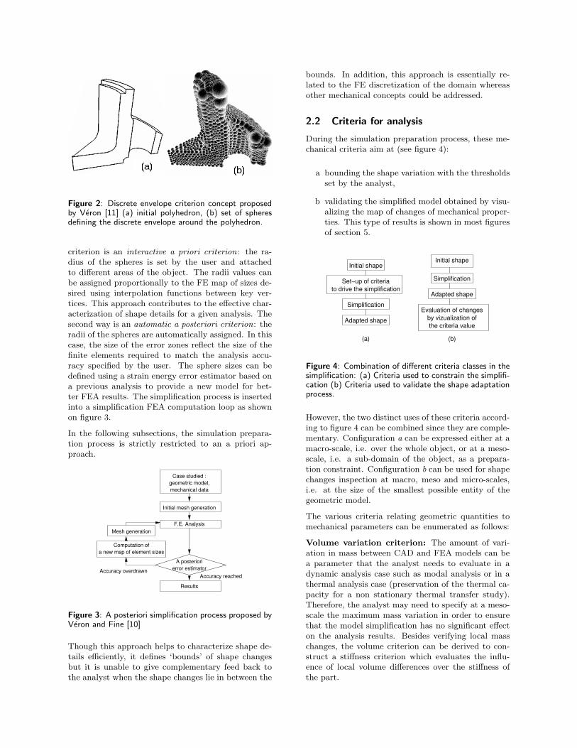
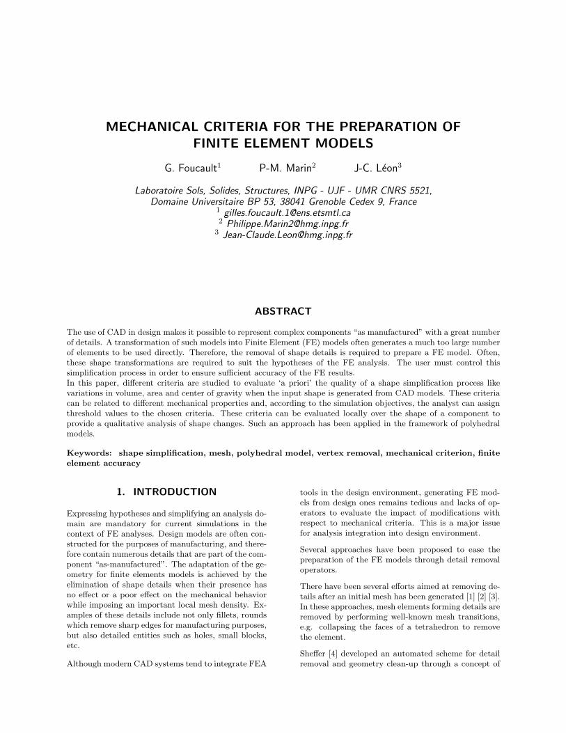
Figure 2: Discrete envelope criterion concept proposedby Veron [11] (a) initial polyhedron, (b) set of spheresdefining the discrete envelope around the polyhedron.
criterion is an interactive a priori criterion: the ra-dius of the spheres is set by the user and attachedto different areas of the object. The radii values canbe assigned proportionally to the FE map of sizes de-sired using interpolation functions between key ver-tices. This approach contributes to the effective char-acterization of shape details for a given analysis. Thesecond way is an automatic a posteriori criterion: theradii of the spheres are automatically assigned. In thiscase, the size of the error zones reflect the size of thefinite elements required to match the analysis accu-racy specified by the user. The sphere sizes can bedefined using a strain energy error estimator based ona previous analysis to provide a new model for bet-ter FEA results. The simplification process is insertedinto a simplification FEA computation loop as shownon figure 3.
In the following subsections, the simulation prepara-tion process is strictly restricted to an a priori ap-proach.
Mesh generation
Computation ofa new map of element sizes
Initial mesh generation
A posteriorierror estimator
Case studied :geometric model,mechanical data
F.E. Analysis
Results
Accuracy reachedAccuracy overdrawn
Figure 3: A posteriori simplification process proposed byVeron and Fine [10]
Though this approach helps to characterize shape de-tails efficiently, it defines ‘bounds’ of shape changesbut it is unable to give complementary feed back tothe analyst when the shape changes lie in between the
bounds. In addition, this approach is essentially re-lated to the FE discretization of the domain whereasother mechanical concepts could be addressed.
2.2 Criteria for analysis
During the simulation preparation process, these me-chanical criteria aim at (see figure 4):
a bounding the shape variation with the thresholdsset by the analyst,
b validating the simplified model obtained by visu-alizing the map of changes of mechanical proper-ties. This type of results is shown in most figuresof section 5.
Initial shapeInitial shape
Set−up of criteriato drive the simplification
Simplification
Adapted shape
Simplification
Adapted shape
Evaluation of changesby vizualization ofthe criteria value
(a) (b)
Figure 4: Combination of different criteria classes in thesimplification: (a) Criteria used to constrain the simplifi-cation (b) Criteria used to validate the shape adaptationprocess.
However, the two distinct uses of these criteria accord-ing to figure 4 can be combined since they are comple-mentary. Configuration a can be expressed either at amacro-scale, i.e. over the whole object, or at a meso-scale, i.e. a sub-domain of the object, as a prepara-tion constraint. Configuration b can be used for shapechanges inspection at macro, meso and micro-scales,i.e. at the size of the smallest possible entity of thegeometric model.
The various criteria relating geometric quantities tomechanical parameters can be enumerated as follows:
Volume variation criterion: The amount of vari-ation in mass between CAD and FEA models can bea parameter that the analyst needs to evaluate in adynamic analysis case such as modal analysis or in athermal analysis case (preservation of the thermal ca-pacity for a non stationary thermal transfer study).Therefore, the analyst may need to specify at a meso-scale the maximum mass variation in order to ensurethat the model simplification has no significant effecton the analysis results. Besides verifying local masschanges, the volume criterion can be derived to con-struct a stiffness criterion which evaluates the influ-ence of local volume differences over the stiffness ofthe part.
Center of gravity and inertia: During the simpli-fication of a geometric model, each transformation oncurved areas introduce a displacement of the centerof gravity and a variation in inertia moments. Then,the analyst may need to avoid transformations thatgenerate a displacement of center of gravity over aprescribed threshold distance, or a variation in someinertia matrix values over a given value.
Such a criterion is meaningful both for volumes, freeform surfaces, as well as planar sections when consid-ering beam-shaped components.
Area variation criterion: In several cases, the vari-ation in area of a surface is an interesting criterion tomonitor the simplification process.
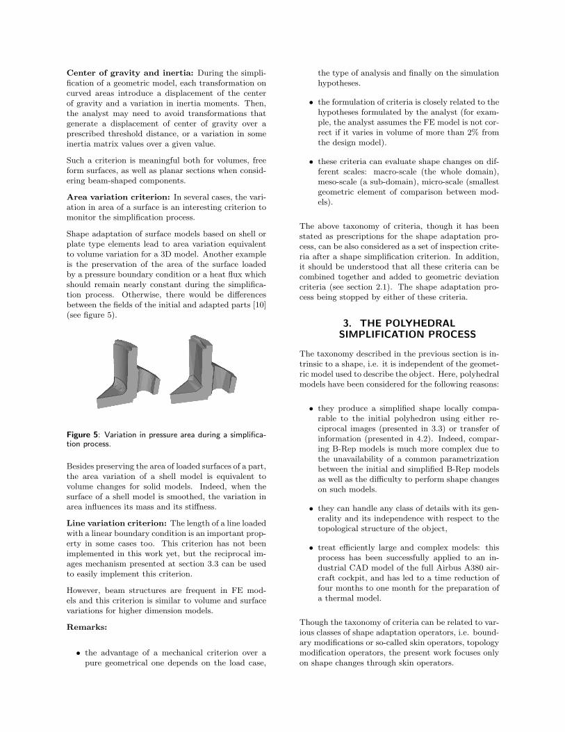
Shape adaptation of surface models based on shell orplate type elements lead to area variation equivalentto volume variation for a 3D model. Another exampleis the preservation of the area of the surface loadedby a pressure boundary condition or a heat flux whichshould remain nearly constant during the simplifica-tion process. Otherwise, there would be differencesbetween the fields of the initial and adapted parts [10](see figure 5).
Figure 5: Variation in pressure area during a simplifica-tion process.
Besides preserving the area of loaded surfaces of a part,the area variation of a shell model is equivalent tovolume changes for solid models. Indeed, when thesurface of a shell model is smoothed, the variation inarea influences its mass and its stiffness.
Line variation criterion: The length of a line loadedwith a linear boundary condition is an important prop-erty in some cases too. This criterion has not beenimplemented in this work yet, but the reciprocal im-ages mechanism presented at section 3.3 can be usedto easily implement this criterion.
However, beam structures are frequent in FE mod-els and this criterion is similar to volume and surfacevariations for higher dimension models.
Remarks:
• the advantage of a mechanical criterion over apure geometrical one depends on the load case,
the type of analysis and finally on the simulationhypotheses.
• the formulation of criteria is closely related to thehypotheses formulated by the analyst (for exam-ple, the analyst assumes the FE model is not cor-rect if it varies in volume of more than 2% fromthe design model).
• these criteria can evaluate shape changes on dif-ferent scales: macro-scale (the whole domain),meso-scale (a sub-domain), micro-scale (smallestgeometric element of comparison between mod-els).
The above taxonomy of criteria, though it has beenstated as prescriptions for the shape adaptation pro-cess, can be also considered as a set of inspection crite-ria after a shape simplification criterion. In addition,it should be understood that all these criteria can becombined together and added to geometric deviationcriteria (see section 2.1). The shape adaptation pro-cess being stopped by either of these criteria.
3. THE POLYHEDRALSIMPLIFICATION PROCESS
The taxonomy described in the previous section is in-trinsic to a shape, i.e. it is independent of the geomet-ric model used to describe the object. Here, polyhedralmodels have been considered for the following reasons:
• they produce a simplified shape locally compa-rable to the initial polyhedron using either re-ciprocal images (presented in 3.3) or transfer ofinformation (presented in 4.2). Indeed, compar-ing B-Rep models is much more complex due tothe unavailability of a common parametrizationbetween the initial and simplified B-Rep modelsas well as the difficulty to perform shape changeson such models.
• they can handle any class of details with its gen-erality and its independence with respect to thetopological structure of the object,
• treat efficiently large and complex models: thisprocess has been successfully applied to an in-dustrial CAD model of the full Airbus A380 air-craft cockpit, and has led to a time reduction offour months to one month for the preparation ofa thermal model.
Though the taxonomy of criteria can be related to var-ious classes of shape adaptation operators, i.e. bound-ary modifications or so-called skin operators, topologymodification operators, the present work focuses onlyon shape changes through skin operators.

The adaptation of the shape is applied to an interme-diate polyhedral model generated from a CAD modeland is based on the identification of geometric areaswhose removal or modification enables the simplifica-tion of the simulation model (decrease of the number ofvertices), without affecting the simulation results. Thezones considered as “details” are therefore zones wherethe discretisation generates a large number of nodeswhich are unnecessary to ensure acceptable simulationresults. It is assumed here that the input polyhedronhas a discretization compatible with the requirementsof the map of FE sizes expressed by the analyst, i.e.in curved areas the edge length is smaller than thetarget FE edge length and in directions of null curva-tures the edge length can be greater than the targetFE size. Such a configuration preserves the consis-tency with the FE map of sizes criterion described atsection 2.1, enables the reduction of the model com-plexity while avoiding adverse effects on the target FEmesh, as pointed out by Owen [12].
3.1 Overview of the skin operator
The simplification process of a polyhedral model onwhich the proposed mechanical criteria is briefly re-viewed hereunder. The input data of the simplifica-tion process is a polyhedral model of the part. Thesimplification process is based on an iterative vertexremoval algorithm. First, the edges and vertices of theinitial polyhedral model are classified in accordanceto their topological information. This classification isnecessary to apply the appropriate selection criterionand vertex removal operators to each class of vertices:boundary entities, surface entities, unremovable enti-ties, ...
Then, the simplification treatment is initialized. Aspherical error zone is assigned to each vertex of theinput model. The radius of these spheres can be setup using an a priori or a posteriori mechanical crite-rion (see section 2.1). At each face an inheritance pro-cess of error zones is performed to monitor the shaperestoration during the simplification process. As illus-trated in figure 1, the spherical error zone criterion aimat simplifying the geometry according to the elementsize chosen by the analyst, using his a priori expertiseof the simulation needs. The mechanical criteria pro-posed here act in this part of the algorithm. Therefore,local volume variation, local area variation, center ofgravity deviation, ..., are monitored and used as a pri-ori criteria at this stage of the algorithm. Maximumallowed values of volume variation, area variation, orcenter of gravity deviation can be assigned interac-tively to a set of faces of the initial polyhedral model.Once the simplification criteria has been set, the sim-plification process starts, and a loop is executed untilno more candidate vertex can be removed.
At each iteration of the process, a vertex removal op-erator is applied to create a new local geometry from
(a) (b)
(c)
(d)
Star polyhedron Contour polygon Remesh
Figure 6: Vertex removal operator: (a) star-shaped poly-hedron around the candidate vertex and initial polyhe-dron, (b) hole created for star polyhedron removal andits corresponding contour polygon, (c) candidate remesh-ing of contour polygon created, (d) the remeshing andthe final polyhedron.
the contour polygon of this vertex (see fig. 6). Thisnew set of faces covering the contour polygon is de-fined by the remeshing scheme selected. The set offaces around the candidate vertex is called the star-shaped polyhedron. Each criterion assigned by theuser is then applied to determine whether or not thevertex can be removed. If the mechanical properties ofthe initial model are correctly restored, the faces of thestar-shaped polyhedron are replaced by the appropri-ate remeshing created by the vertex-removal operatoras shown on figure 6.
The remeshing scheme of the star polyhedron is pro-cessed by optimising element shape criteria. The iter-ative application of the vertex removal operator tendsto smooth the global shape of the polyhedron, andthen, tends to remove small and curved shape detailswhich are irrelevant details as shown on figure 7.
(a) (b)
Figure 7: Solid model containing many skin details (a)initial polyhedron, (b) coarse model obtained using theiterative vertex removal operator.
The simplified shape obtained from this process formsnow the basis of a FE mesh generation process. How-ever, under appropriate criteria (size, form, ...), thisprocess can produce directly the target FE mesh [13].The influence of this operator has been evaluated fromthe stress point of view and has produced satisfactoryresults when comparing the results obtained from theinitial geometry and the simplified geometry generatedfrom an enveloppe produced by an a posteriori errorestimator [14].
3.2 Structure of a geometric criterion
All the criteria listed previously (see section 2.2) neednow to be evaluated using the vertices, edges and facesof the polyhedral model. Hence, the local geometricquantities required are reduced to a face, an edge or avertex.
The evaluation of changes at the local scale is nec-essarily based on a representation of some geometricelements of the initial shape and their image on thesimplified one, i.e. a mapping.
In our work, the method of comparison between poly-hedrons characterizes the two approaches proposed inthis work: while the propagation approach is basedon the differences between the star polyhedron and itsassociated remeshing at each step of the skin detail re-moval operator, the cell-based approach relies on thedifference between the remeshing and its “mapping”on the initial polyhedron.
Many configurations arise when one try to calculatethe geometric projection of one polyhedron onto an-other as illustrated in figures 8 and 10.
(a) (b)
(c) (d)
?
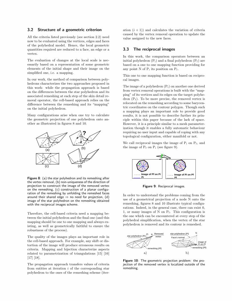
Figure 8: (a) the star polyhedron and its remeshing afterthe vertex removal, (b) non-uniqueness of the direction ofprojection to construct the image of the removed vertexon the remeshing, (c) construction of a planar configu-ration of the remeshing by unfolding the remeshed facesaround their shared edge ⇒ no need for projection, (d)image of the star polyhedron on the remeshing obtainedwith the reciprocal images scheme.
Therefore, the cell-based criteria need a mapping be-tween the initial polyhedron and the final one (and thismapping should be one to one mapping and always ex-isting, as well as geometrically faithful to ensure therobustness of the process).
The quality of the images plays an important role inthe cell-based approach. For example, any shift or dis-tortion of the image will produce erroneous results oncriteria. Mapping and bijection characterize aspectsrelated to parametrization of triangulations [15] [16][17] [18].
The propagation approach transfers values of criteriafrom entities at iteration i of the corresponding starpolyhedron to the ones of the remeshing scheme (iter-
ation (i + 1)) and calculates the variation of criteriacaused by the vertex removal operation to update thevalue assigned to the new faces.
3.3 The reciprocal images
In this work, the comparison operators between aninitial polyhedron (Pi) and a final polyhedron (Pf) arebased on a one to one mapping function providing forany point N of Pi its position on Pf .
This one to one mapping function is based on recipro-cal images.
The image of a polyhedron (Pi) on another one derivedfrom vertex removal operations is built with the “map-ping” of its vertices and its edges on the target polyhe-dron (Pf). To be more precise, the removed vertex isrelocated on the remeshing according to some barycen-tric coordinates on the contour polygon. Though sucha mapping plays an important role to provide goodresults, it is not possible to describe further its prin-ciple within this paper because of the lack of space.However, it is a principle similar to a mesh parameter-ization though it enables a fully automatic behaviourrequiring no user input and capable of coping with anytopological configuration, either manifold or not.
We call reciprocal images the image of Pi on Pf , andthe image of Pf on Pi (see figure 9).
Image of Pi on PfPf
Image of Pf on PiPi
Figure 9: Reciprocal images.
In order to understand the problems coming from theuse of a geometrical projection of a node N onto theremeshing, figures 8 and 10 illustrate typical configu-rations. Indeed, in the general case, there can exist 0,1, or many images of N on Pf . This configuration isthe one which can be encountered at every step of thepolyhedral simplification, when the vertex of the starpolyhedron is removed and its contour is remeshed.
Pi Removedvertex
remeshing (Pf)
star polyhedron (Pi)N
remeshing (Pf)
N
Face's normal
star polyhedron (Pi)
image of Pi on Pf
a) b)
Figure 10: The geometric projection problem: the pro-jection of the removed vertex is localized outside of theremeshing.

Using the above principle of reciprocal images duringthe skin detail removal process provides an appropri-ate and robust mapping for transferring criteria valuesduring the shape changes.
4. APPROACHES FOR CRITERIAEVALUATION
All mechanical criteria presented in section 2 arefounded on local variation in volume, area, center ofgravity displacement, and inertia moments of the poly-hedral model.
This section presents two different approaches for thecalculation of the basic quantities related to these cri-teria:
• The first approach, called cell-based approach, isan exact calculation of the local value of the cri-teria since it relies on an exact representation ofthe local difference between the two polyhedrons.To achieve the exact representation of the localdifference, this approach is based on reciprocalimages presented in section 3.3 which are geo-metrically faithful and don’t ‘slide’ on the tar-get polyhedron. Currently, the computation costof the reciprocal images is about four times thevertex-removal operator cost.
• The second approach called propagation approachis based on the information propagation througheither faces or nodes during the vertex removalprocess, without use of the reciprocal images.This approach is faster and can be used to han-dle polyhedrons which contain a large number offaces.
Both approaches are suited to inspection purposessince their use is rather qualitative. Though the firstapproach is more suitable since there is no approxi-mation, both approaches are equivalent from the pre-scriptive point of view since they evaluate differentvalues summing up to the same global quantity overthe polyhedron.
4.1 Cell-based approach
The principle of this method is to construct locally onthe polyhedron Pi (or Pf) the solid model of the spacebetween itself and the other polyhedron Pf (or Pi) asillustrated in figures 10, 11, and 12.
In order to clearly express the algorithms, some ter-minology and symbols are given at this point:
• Fi and Ff symbolize a face of the initial poly-hedron Pi and a face of the final polyhedron Pf
respectively. The image of Fi on Pf lies partlyin Ff and reciprocally the image of Ff on Pi liespartly in Fi.
• A cell is defined by the image of Ff on Fi and bythe image of Fi on Ff . We call Ci the polygonalshape representing the image of Fi on Ff and Cf
the image of Fi on Ff as shown in figure 11.
A cell is the image of a face of Pi (or Pf) on a face ofPf (or Pi). The figure 11 shows the construction of acell.
(a)
(b)(c)
Ff image of Fi
image of Ffcell on Pi
Ficell on Pf
Pf (final polyhedron)
Pi (initialpolyhedron)
Figure 11: Illustration of a cell: (a) image of a face ofPi on Pf ,(b) image of a face Pf on Pi, (c) constructionof a cell from both images.
The cell concept represents geometrically and accu-rately the elementary variations resulting from thesimplification process. The set of cells having an imageon a face of Pf represents the total variation betweenthis face and Pi. Therefore, the set of solid volumesof cells having an image on a face of Pf represents thetotal volume difference between this face and Pi. Thisproperty is illustrated on figure 12.
Figure 12: Set of cells having an image on a face of Pf :the assembly of the set represents the volume variationlying on the face of Pf .
4.1.1 Algorithm for cells construction
Each cell is represented by the following data struc-ture:
• The identifiers of its associated faces Ff and Fi,
• Its images Cf and Ci on Pf and Pi respectively.
Cells are constructed from reciprocal images using thefollowing algorithm:
for each face Fi of Pi doGet the three oriented edges of Fi
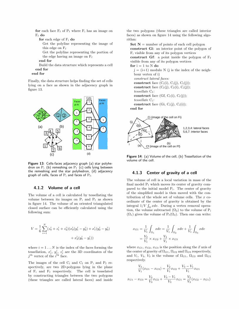
for each face Ff of Pf where Fi has an image onFf do
for each edge of Fi doGet the polyline representing the image ofthis edge on Ff
Get the polyline representing the portion ofthe edge having an image on Ff
end forBuild the data structure which represents a cell
end forend for
Finally, the data structure helps finding the set of cellslying on a face as shown in the adjacency graph infigure 13.
1 12
234
3 4
12
5
6
(a) (b)
(c)
1
2
3
4
1
2
1
2
3
4
5
6
Facesof Pi
Facesof Pf
Cells
(d)
Figure 13: Cells-faces adjacency graph (a) star polyhe-dron on Pi (b) remeshing on Pf (c) cells lying betweenthe remeshing and the star polyhedron, (d) adjacencygraph of cells, faces of Pi and faces of Pf .
4.1.2 Volume of a cell
The volume of a cell is calculated by tessellating thevolume between its images on Pi and Pf as shownin figure 14. The volume of an oriented triangulatedclosed surface can be efficiently calculated using thefollowing sum:
V =1
6
NXi=1
(zi0 + zi
1 + zi2)(x
i0(y
i1 − yi
2) + xi1(y
i2 − yi
0)
+ xi2(y
i0 − yi
1))
where i = 1 . . . N is the index of the faces forming thetessellation, xi
j , yij , zi
j are the 3D coordinates of thejth vertex of the ith face.
The images of the cell Ci and Cf on Pi and Pf re-spectively, are two 2D-polygons lying in the planeof Fi and Ff respectively. The cell is tesselatedby constructing triangles between the two polygons(these triangles are called lateral faces) and inside
the two polygons (these triangles are called interiorfaces) as shown on figure 14 using the following algo-rithm:
Set N = number of points of each cell polygonconstruct Gi: an interior point of the polygon ofFi visible from any of its polygon verticesconstruct Gf : a point inside the polygon of Ff
visible from any of its polygon verticesfor i = 1 to N do
j = (i+1) modulo N (j is the index of the neigh-bour vertex of i)construct lateral faces:construct face (Ci(i), Ci(j), Cf(j));construct face (Cf(j), Cf(i), Ci(j));tessellate Cf :construct face (Gf, Cf(i), Cf(j));tessellate Ci:construct face (Gi, Ci(j), Ci(i));
end for
1,2,3,4: lateral faces5,6,7: interior faces
(b)
1
7 6
2
34
5
i
ij
j
Gf
Gi
Ci (image of the cell on Fi)
Cf (image of the cell on Ff)(a)
Figure 14: (a) Volume of the cell, (b) Tessellation of thevolume of the cell.
4.1.3 Center of gravity of a cell
The volume of cell is a local variation in mass of thefinal model Pf which moves its center of gravity com-pared to the initial model Pi. The center of gravityof the simplified model is then moved with the con-tribution of the whole set of volume cells. The x co-ordinate of the center of gravity is obtained by theintegral 1/V
RΩ
xdv. During a vertex removal opera-tion, the volume subtracted (Ω2) to the volume of Pi
(Ω1) gives the volume of Pf(Ω3). Then one can write:
xG1 =1
V1
ZΩ1
xdv =1
V1
ZΩ2
xdv +1
V1
ZΩ3
xdv
=V2
V1× xG2 +
V3
V1× xG3
where xG1, xG2, xG3 is the position along the ~x axis ofthe center of gravity of ΩG1, ΩG2 and ΩG3 respectively,and V1, V2, V3 is the volume of ΩG1, ΩG2 and ΩG3
respectively.
V3
V1(xG1 − xG3) =
V2
V1xG2 +
V3 − V1
V1xG1
xG1 − xG3 =V2
V3xG2 +
V3 − V1
V3xG1 =
V2
V3(xG2 − xG1)

the displacement of the center of gravity is:
xG1 − xG3 = V2/V3(xG2 − xG1)
where the index 2 corresponds to the subtracted solidvolume, the index 1 to Pi, and the index 3 to Pf .
Thus, one needs to calculate the position of the centerof gravity for Pi and, for the subtracted volume, toobtain the position of the center of gravity of Pf . Theposition of the center of gravity of a tessellated closedsurface can be efficiently calculated using the followingsum:
xG =1
24V
NXi=1
“xi
02
+ xi12
+ xi22
+ xi0x
i1 + xi
1xi2 + xi
2xi0
”×
“(yi
1 − yi0)(z
i2 − zi
0)− (yi2 − yi
0)(zi1 − zi
0)”
where i = 1 . . . N is the index of the faces defining thetessellation, xi
j , yij , zi
j are the 3D coordinates of thejth vertex of the ith face.
The tessellation used for the center of gravity calcu-lation is the one introduced in paragraph 4.1.2 and infigure 14.
4.1.4 Area of a cell
The area of a cell enables the calculation of the localexpansion of the surface. Then, the area of Ci and Cf
are calculated and the area expansion ratioSf−Si
Sfcan
be used to control the simplification.
The area of Ci and Cf is calculated by tessellating thepolygons with interior faces using the principle of para-graph 4.1.2 shown in figure 14. The area of both cellimages is then calculated by summing up the triangleareas.
4.2 Information propagation based ap-proach
The simplification is obtained by the iterative vertexremoval operation. At every step of this process, den-sity informations can be assigned to the faces or ver-tices and transfered by inheritance during the simpli-fication process.
This information transfer approach provides an ap-proximative value of the initial information.
4.2.1 Propagation through vertices
This propagation method consists in assigning infor-mations of local area and volume variations to the ver-tices of the polyhedron. At each step of the process,the informations assigned to the vertex removed areinherited by the vertices of the contour of the starpolyhedron.
For every vertex removal operation, the algorithm usedis:
1. calculation of the volume subtracted between thestar polyhedron and its remeshing as shown infigure 15. Because the faces of this volume aretriangular, the calculation of the volume does notneed a tessellation of the volume, and the volumeis directly obtained using formula 4.1.2.
2. calculation of the area of the star polyhedron andof its remeshing.
3. inheritance from the information attached to theremoved vertex to the vertices of the remeshingcontour. Area and volume information are up-dated by weighting the value of the removed ver-tex proportionally to the inverse of the distancebetween this vertex and one of the contour vertex:
∆Vi =
1diPN
j=11dj
×(∆Vstar poly. + ∆Vremoved vertex)
where di is the distance between the removed ver-tex and the contour vertex, and ∆Vi is the valueto be added to the information of the ith contourvertex.
Figure 15: Volume variation produced by the vertex re-moval operation
4.2.2 Propagation through faces
This propagation scheme is similar to the propagationthrough vertices presented in 4.2.1. At each step ofthis process, density informations can be assigned tothe faces and inherited from the N initial faces, i.e.the star polyhedron faces, to the (N − 2) final faces,i.e. the remeshing faces, according to their area.
For every vertex removal operation, the algorithm usedis:
1. calculation of the volume subtracted between thestar polyhedron and the remeshing as shown infigure 15.
2. calculation of the areas of the star polyhedronand of the remeshing.
3. the total volume and area variations are dis-tributed on each face of the remeshing propor-tionally to their areas, with the sum of:

(a) the area and volume variation informationsinherited from the faces of the star polyhe-dron,
(b) and the area and volume variations causedby the vertex removal operation.
This sum writes:
∆Vfinal =
NXi=1
δVi + ∆Vstar
=
N−2Xj=1
δVj + ∆Vstar
where δVj =Sj
Sremesh∆Vremesh
where δVi is the information inherited from thestar polyhedron, i is the index of the faces of thestar polyhedron, and j is the index of the facesof the remeshing. Similarly, it comes for the areavariation:
∆Sfinal =
NXi=1
(αiSi) + ∆Sstar
=
N−2Xj=1
(αjSj) + ∆Sstar
where αj =Sj
Sremesh∆Sremesh.
5. EXAMPLES AND RESULTS
Model Faces Edges Vertices
Bracket 1824 2736 908
Sub-domain 4302 6453 2750
Head 1374 2061 689
Figure 16: Characteristics of the test models
The algorithms were implemented as part of the Sim-poly1 software. The implementation of the reciprocalimages and cell-based approaches for our a priori crite-ria was used to evaluate the simplification results andto monitor the simplification process.
The results are illustrated below through several ex-amples representing different shapes.
The criteria aim at verifying whether a simplificationis acceptable or not according to the threshold valueset by the analyst. However, this configuration of pre-scriptive use of the criteria is difficult to illustrategraphically. Hence, the proposed illustration of thecriteria are based on their inspection usage, i.e. af-ter a simplification operation, the analyst is able toevaluate how the volume or area or center of gravitylocation of the simplified model has evolved.
1this software consists in a polyhedral approach for anal-ysis model preparation, featuring conformity set-up, skinand topological detail removal, idealization.
The local values of criteria are updated at each step ofthe iterative vertex removal process. A remeshing ofthe star polyhedron contour is rejected if some of theprevious criteria listed violates a threshold value.
The computation of criteria with the cell-based ap-proach provides robust and accurate results. Thisquality is mainly due to the fact that the calculation isbased on an exact geometric representation of the lo-cal differences between the initial polyhedron and thesimplified one.
However, the cell-based approach remains slower thanthe information propagation-based approach becauseof the computation cost of reciprocal images, of thecell construction and criteria evaluation. Since the re-ciprocal images are modified only over the star poly-hedron of the vertex removed, the only informationsto update at each step of the vertex removal operatorare the cells adjacent to this star polyhedron. Then,the differences of volume or area lying on a set of theinitial polyhedron faces can be efficiently monitored tosatisfy a simplification value set by the analyst.
Processing large models (number of faces greater than105) is often needed, and the computation cost of re-ciprocal images is about four times the sole vertex re-moval one. The latter being around 25% slower thanthe commercial decimation software.
The results obtained with the information propaga-tion approaches highlight an approximation of the mapof densities of volume and area variations. The re-sults obtained with the propagation through nodes(fig. 17, 18, 19), and with the propagation throughfaces (fig. 19) are compared to the results obtainedwith the cell-based approach. The comparison of theseresults clearly highlights the approximation effects ofthe propagation through vertices or faces. These ap-proximations create a smoothing effect which can leadto inappropriate interpretation of the simplificationoperation. Because in both categories of approaches(cell-based and information propagation) the cumula-tive values sum up to the same value prescribed bythe user, the information propagation approach seemsmore suited to prescriptive uses only of the criteriasince their computation time is better than the cell-based approach. However, if the criteria are used bothin prescriptive and inspection configurations, the cell-based approach should be preferred because of its bet-ter restitution of the simplification effects.
The models in figure 17 are colorized with the den-sities of volume differences computed for each face ofthe final polyhedron. One can see that the curved sur-faces have the highest differences. The differences arepositive in the convex regions where some material hasbeen removed (yellow and red colored areas), and neg-ative in the concave regions where some material hasbeen added (blue colored areas).
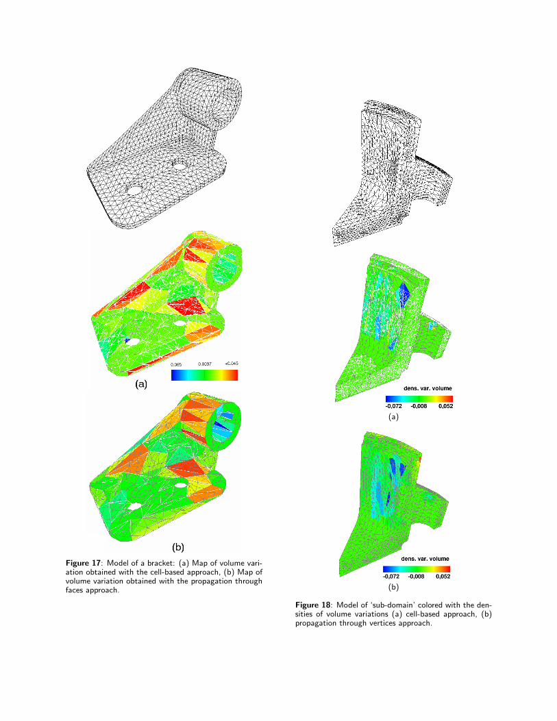
Figure 17: Model of a bracket: (a) Map of volume vari-ation obtained with the cell-based approach, (b) Map ofvolume variation obtained with the propagation throughfaces approach.
(a)
(b)
Figure 18: Model of ‘sub-domain’ colored with the den-sities of volume variations (a) cell-based approach, (b)propagation through vertices approach.

On this bracket (fig. 19), the results of volume varia-tions obtained by propagation through vertices high-light quasi null values in the neighbourhood of the twoholes (see figure 19 (c)). These values should be morevisible as depicted on the solution obtained with thecell-based approach in figure 19 (a)). The approach ofpropagation through faces provide better results in theneighbourhood of the holes as shown in figure 19(b).
Figure 19: Map of volume variation on the bracket model(a) cell-based approach, (b) propagation through facesapproach, (c) propagation through vertices approach.
Another criterion can be illustrated using the followingexample to illustrate how they can be related to beam-shaped components through sections. Here, the crite-rion set up characterizes the area variation of beamsections. The sections are defined through referenceplanes and interpolation criteria between them. Thefigure 20 illustrates the variation of contours duringthe simplification process: contracted and expandedsections are colored in blue and red respectively. Here,the principle is based on the calculation of the inter-section between each plane defining a section and thefaces of the polyhedral model.
Figure 20: Principle of the section area variation crite-rion.
The figure 21 shows the contraction of many faceson the final polyhedron compared to the initialpolyhedron.
Figure 21: Vizualization of the surfacic densities of vari-
ation in areaSfinal−Sinit.
Sfinalon a human head model ob-
tained with the cell-based approach.

6. CONCLUSION AND FUTURE WORK
In the context of FE model preparation, this work hasproposed a set of criteria for monitoring the shapeadaptation process of design models. These criteriaare linked to mechanical properties such as mass, area,stiffness, and have been expressed for a polyhedral rep-resentation of the structure.
Two classes of approach have been used to assess thesecriteria: the most rigorous one based on reciprocalimages and an approximate one. The methods are es-pecially well-suited to constrain the polyhedral modelsimplification locally for the needs of the analysis ap-plication. They are designed to be used simultaneouslywith the discrete envelope criterion proposed by Veron[11] and Fine [10]. Currently, these methods enable usto:
• simplify a model while preserving its physicalproperties and avoiding transformations whichimply a variation in some physical propertygreater than the threshold set by the analyst,
• visualize and evaluate the physical propertiespreservation at the end of a simplification op-eration before starting the FE mesh generationphase.
Among the two propagation schemes tested for thepropagation approach, the propagation through facesis the best suited to reliably spread the criteria valuesover the component.
The cell-based approach gives accurate results of thecriteria values but is slower than the propagationschemes. Mixing both approaches over the shape ofthe object according to user prescriptions can improvefurther the performance of these criteria.
The ability of criteria to preserve mechanical proper-ties relevant for some analysis has been discussed andevaluated but work on other criteria are planed to com-plete the simplification process. Future work will focuson the completeness of these criteria and their combi-nation strategies. Complementary a priori criteria likeshape of sections, stiffness, will be developed to leadto a performant solution for conversion from designmodels to structural analysis models. Ongoing workfocuses on transfering CAD data conveying semanticsabout a model to the polyhedral model, thus leadingto the notion of simplification features to incorporatefurther constraints.
References
[1] Dey S., Shephard M.S., Georges M.K. “Elimina-tion of the Adverse Effects of Small Model Fea-tures by the Local Modification of AutomaticallyGenerated Meshes.” Engineering with Comput-ers, vol. 13, no. 3, 134–152, 1995
[2] Shephard M.S., Beall M.W., O’Bara R.M. “Re-visiting the Elimination of the Adverse Effectsof Small Model Features in Automatically Gen-erated Meshes.” 7th International MeshingRoundtable, pp. 119–132. 1998
[3] Mark W. Beall Joe Walsh M.S.S. “AccessingCAD geometry for mesh generation.” Proceed-ings of 12th International Meshing Roundtable,Sandia National Laboratories. 2003
[4] Sheffer A., Blacker T., Bercovier M. “Cluster-ing: Automated detail suppression using virtualtopology.” vol. 220, pp. 57–64. ASME, 1997
[5] Blacker T., Sheffer A., Clements J., Bercovier M.“Using virtual topology to simplify the mesh gen-eration process.” vol. 220, pp. 45–50. ASME, 1997
[6] Mobley A.V., Carroll M.P., Canann S.A. “An Ob-ject Oriented Approach to Geometry Defeaturingfor Finite Element Meshing.” 7th InternationalMeshing Roundtable, Sandia National Labs, pp.547–563. 1998
[7] Venkataraman S., Sohoni M., Elber G. “Blendrecognition algorithm and applications.” Proceed-ings of the sixth ACM symposium on Solid mod-eling and applications, pp. 99–108. ACM Press,2001
[8] Donaghy R., Armstrong C., Price M. “Dimen-sional Reduction of Surface Models for Analysis.”Engineering with Computers, vol. 16, no. 1, 24–35, 2000
[9] Armstrong C.G. “Modelling requirements forfinite-element analysis.” Computer Aided Design,vol. 26, no. 7, 573–578, 1994
[10] Fine L., Remondini L., Leon J.C. “Automatedgeneration of FEA models through idealizationoperators.” International Journal for NumericalMethods in Engineering, vol. 49, no. 1, 83–108,2000
[11] Veron P., Leon J.C. “Shape preserving polyhedralsimplification with bounded error.” Computers &Graphics, , no. 22, 565 – 585, 1998
[12] Owen S., White D., Tautges T.J. “Facetbasedsurfaces for 3D mesh generation.” Proceedings of11th Int. Meshing Roundtable, pp. 297–311. 2002
[13] Fine L., Leon J.C. “A new approach to the Prepa-ration of models for F.E. analyses.” InternationalJournal of Computer and Applications, vol. to ap-pear, 2004
[14] Fine L., Remondini L., Leon J.C. “A Control Cri-terion Dedicated to Detail Removal for FEA Ge-ometry Adaptation.” P. Chedmail, et al., editors,Proceedings of Integrated Design and Manufactur-ing in Mechanical Engineering. Kluwer, 2002
[15] Sheffer A., Sturler E.D. “Surface Parameter-ization for Meshing by Triangulation Flatten-ing.” Proceedings of 9th International MeshingRoundtable, pp. 161–172. 2000
[16] Desbrun M., Meyer M., Alliez P. “IntrinsicParameterizations of Surface Meshes.” Com-puter Graphics Forum, vol. 21, pp. 209–218. 23rdAnnual Conference (EUROGRAPHICS 2002),Blackwell Science Ltd, Saarbrucken, Germany,Sep 2002
[17] Floater M.S. “Parametrization and smooth ap-proximation of surface triangulations.” ComputerAided Geometric Design, vol. 14, no. 3, 231–250,April 1997
[18] Gotsman C., Gu X., Sheffer A. “Fundamentalsof Spherical Parameterization for 3D Meshes.”ACM Siggraph. July 2003