measuring retiming responses of passengers to a prepeak
TRANSCRIPT

Research ArticleMeasuring Retiming Responses of Passengers toa Prepeak Discount Fare by Tracing Smart Card DataA Practical Experiment in the Beijing Subway
Qingru Zou12 Xiangming Yao 2 Peng Zhao2 Zijia Wang 3 and Taoyuan Yang 3
1School of Traffic and Transportation Shijiazhuang Tiedao University Shijiazhuang Hebei 050043 China2School of Traffic and Transportation Beijing Jiaotong University No 3 Shangyuancun Haidian District Beijing 100044 China3School of Civil Engineering Beijing Jiaotong University No 3 Shangyuancun Haidian District Beijing 100044 China
Correspondence should be addressed to Xiangming Yao yaoxmbjtueducn
Received 19 December 2018 Revised 28 March 2019 Accepted 15 May 2019 Published 4 June 2019
Academic Editor Rocıo de Ona
Copyright copy 2019 Qingru Zou et al This is an open access article distributed under the Creative Commons Attribution Licensewhich permits unrestricted use distribution and reproduction in any medium provided the original work is properly cited
Understanding passengersrsquo responses to fare changes is the basis to design reasonable price policies This work aims to exploreretiming responses of travelers changing departure times due to a prepeak discount pricing strategy in the Beijing subway inChina using smart card records from an automatic fare collection (AFC) system First a new set of classification indicators isestablished to segment passengers through a two-step clustering approach Then the potentially influenced passengers for the farepolicy are identified and the shifted passengers who changed their departure time are detected by tracing changes in passengersrsquoexpected departure times before and after the policy Lastly the fare elasticity of departure time is defined to measure the retimingresponses of passengers Two scenarios are studied of one month (short term) and six months (middle term) after the policy Theretiming elasticity of different passenger groups retiming elasticity over time and retiming elasticity functions of shifted timeare measured The results show that there are considerable differences in the retiming elasticities of different passenger groupslow-frequency passengers are more sensitive to discount fares than high-frequency passengers The retiming elasticity decreasesgreatly with increasing shifted time and 30 minutes is almost the maximum acceptable shifted time for passengers Moreover theretiming elasticity of passengers in the middle term is approximately twice that in the short term Applications of fare optimizationare also executed and the results suggest that optimizing the valid time window of the discount fares is a feasible way to improvethe congestion relief effect of the policy while policy makers should be cautious to change fare structures and increase discounts
1 Introduction
11 Motivation The Beijing subway is suffering from seriouscongestion due to booming travel demand especially duringthe morning peak hours (700 amsim900 am) To relieveovercrowding transit agencies implemented a discount pric-ing measure in 2016 that provided a 30 discount forpassengers who checked in before 700 am It was the firstcase in China to use time-dependent pricing policy in railtransit systems and the measure was only a pilot policyat certain stations After one year of the experiment thediscount rose from 30 to 50 and the number of trialstations increased from 16 to 23 However the policy is stillin the pilot stage and is not expanding to a larger scale
because the responses of passengers to the discount fareremain unclear and no obvious reduction in peak demandis observed
Differential pricing is an important and effective measurein traffic demand management (TDM) Whether pricingstrategies work depends strongly on the responses of travelersto fare changes Normally the fare elasticity of demand isused to describe the relationship between demand changesand fare changes at an aggregate level It is useful to estimatedemand changes for system-wide and long-term pricingpolicies However for regional and short-term (valid timewindow is short) fare strategies it is hard to capture thereactions just by the fare elasticity of demand For instancethe prepeak discount price in the Beijing subway is valid
HindawiJournal of Advanced TransportationVolume 2019 Article ID 6873912 20 pageshttpsdoiorg10115520196873912
2 Journal of Advanced Transportation
only before 700 am which mainly influences passengersrsquodeparture time choices and will not result in obvious changesin demandThere is a great need to consider the microscopictravel responses of passengers to fare changes and thenprovide support to establish a precise pricing scheme
Passengersrsquo travel responses to fare changes are verycomplex and related to various external factors such asservice quality travel preference and socioeconomic factorsPrevious works on travel responses are usually specific to acertain region or transit system and assume that the externalfactors remain the same before and after the policy Unfor-tunately few works on travel responses for transit systems inChina are found as the Beijing subway is the first case to applytime-of-day pricing policy in transit systems Additionallytraditional works are mainly based on statistical methodsusing SPRP (Stated Preference Revealed Preference) surveydata which greatly limits the potential to study passengersrsquotravel responses in depth The RP survey only creates a staticand sampled picture of the traffic pattern in a short timeperiod which introduces errors as peoplersquos travel behaviorchanges over time [1] The SP survey based on fictitioussituations may have large errors because the choices ofinterviewees may be different from their actual behaviorsAs a benefit of the application of the AFC system in railtransit the smart card data produced from the AFC systemprovide valuable insights into the usage of public transportand help to better understand travel demand behavior andother purposes [2] The AFC system not only records theaccurate trip information of each passenger but also makesit possible to track behavior changes of passengers before andafter a new policy
Hence this work aims to explore the retiming behaviorof passengers for departure time choice and determine whichpassengers will travel early and how long they will shift fromtheir original departure time to enjoy the discount fare Themain contributions of this work contain three aspects (1) Anew set of classification indicators which is obtained directlyfrom smart card data is proposed to segment passengersinto groups and then improve the objectivity of classification(2)The shifted passengers who change their departure timeare identified by comparing the expected departure timesbefore and after the fare policy and then the retimingelasticity of different passenger groups retiming elasticityover time and retiming elasticity functions of shifted time aremeasured for the Beijing subway travelers (3) According tothe results of the retiming elasticity the active time thresholdof the discount fare is very short and valid time windowoptimization of the discount price is very important toimprove the effect of the policy
12 Literature Review Passengersrsquo responses to fare changesare usually indicated by demand changes The fare elasticityof demand which is widely used to measure passengersrsquoresponses to fare changes is defined as the percentage changein travel demand due to a 1 change in fare A large numberof case-specific fare elasticities have been studied for trafficand transportation systems Bresson et al noted that theelasticity of transit demand can generally be regarded as -03without considering case-by-case differences [3] However
travel responses are complex and comprehensive behaviorsof passengers not only for price but also related to variousexternal factors Other works have indicated that demandelasticity varies greatly in terms of variables such as age timespan transit mode time of day original fare level incomelevel trip distance data paradigm type and direction of aprice change and demographic and geographic conditions[4ndash8] To reduce the influence of external factors the case-specific fare elasticity should usually be measured whendesigning new fare schemes for a certain traffic system Forrail transit systems Holmgren studied 81 transit fare-changecases and found a price elasticity of demand of -038 [9]while Hensher extracted a value of -0395 from 319 cases [7]Schimek obtained an elasticity of -034 using data collectedfrom 198 transit agencies during 1991 and 2012 [10] Accordingto the data collected in the UK Paulley et al showed thatthe price elasticities of the metro are -026 for peak hourdemand and -042 for off-peak demand Furthermore theyrecommended a range of short-term transit fare elasticitiesof -02 to -05 (-015 to -03 for peak hours) and -037 for themetro in a predicted scenario [11] However considering thelarge variety in the values it has been suggested that a rangerather than an absolute value should be provided for fareelasticities [8] Taking the fare change in the Beijing subwayin 2014 as the background in which a distance-based fare isapplied to replace the flat fare structure Wang et al studiedthe price elasticities of demand bymeans of an SP survey with4210 samples and the values of the price elasticities rangedfrom -0232 to -1143 [12] Furthermore Wang et al studiedthe price elasticities of different distances on weekdays andweekends using smart card data one week before and after afare change [13] Comparing the results of these two worksthe elasticities from the SP survey are much larger thanthose revealed via the smart card data In conclusion thefare elasticities of demand differ greatly for different regionstransit systems and time periods (such as peak and off-peak)It is necessary to measure the fare elasticities for a specifictraffic and transit system when designing new fare schemes
Another approach to measure the travel responses ofpassengers to fare changes is using travel behavior modelsThe fare is treated as a factor that affects the travel behaviorsof passengers such as the departure time choice travel modechoice and travel route choice The most commonly usedtravel behavior models are the logit-based model and itsderivative models Mahmassani et al [14] Lu et al [15 16]and Lu and Mahmassani [17] developed a multicriteria routeand departure time user equilibrium model for dynamictraffic assignment applications with variable toll pricingAboudina et al proposed an integratedmodel by consideringdeparture time choice and travel route choice [18] whileHabib et al integrated departure time choice and travelmode choice [19] Based on these travel behavior modelschanges in demand can be estimated by a traffic assignmentmodel and fare policies can be evaluated through demandchanges [20] Simulations are usually used to examine theaggregate impacts of differential pricingmeasures on a transitor multimodal transport network Liu and Charles notedthat the functionality of a simulation system depends onits core choice model and its assumptions of individualsrsquo
Journal of Advanced Transportation 3
Classification indexes determination
Passenger types analysis
Retiming response measurement
Shied passenger identification
Applications and suggestions
Data preprocessing
AFC database
Passenger
Two-step clustering algorithm
Influenced passenger detection
Passenger classification
Target discount station selection by considering demand structure
Valid time window optimization for discount policy
Retiming elasticity measurementtypes
Figure 1 Framework for studying passengersrsquo retiming responses to the prepeak discount fare
ldquotravel behaviorrdquo eg a travelerrsquos response and sensitivity to apeak fare surcharge alone or combined with changes in otherservice attributes such as onboard crowding and servicefrequency [21] However the heterogeneity and microscopictravel behaviors of passengers can be considered in thesemethods and some necessary attributes in themodel are hardto obtain (such as personal attributes and travel character-istics at the individual level) Due to the lack of advancedand intelligent data acquisition equipment most studies uselimited sample survey data or highly aggregated collectiondata The available data greatly limits the potential to studythe travel responses of passengers in depth
With the wide application of AFC systems in publictraffic and transportation systems massive and continuoustrip information can be obtained The unique ID of smartcards makes it possible to trace day-to-day behavior changesof passengers at the individual level Pelletier et al under-took a complete review of transit smart card research andthey suggested that there was great potential for demandmanagement using card data [22] Compared to survey datasmart card data have outstanding characteristics for travelbehavior analysis such as being accurate continuous andtrackable However there are also intrinsic limitations ofsmart card data including the absence of socioeconomicproperties (age career income homework location etc)and travel information (trip purposes trip chains etc) [2]In recent years many researchers have tried to mine indirectand potential information from smart card data such astravel pattern analysis [23] trip purpose detection [24 25]and travel behavior analysis [26] Although various studies
have been performed on smart card mining the data haverarely been used to study a practical policy Hence takingthe prepeak discount fare in the Beijing subway as thebackground this work aims to study the travel responses ofpassengers for changing departure times for discount faresby tracing the behavior changes of individual passengersthrough the actual trip information from smart card data
13 Organizations Figure 1 provides the framework for ana-lyzing the retiming responses of travelers under a prepeakdiscount price policy There are two important parts ofthis work passenger classification and retiming responsemeasurement Though detailed trip information (such astravel time origin-destination and fare) for each cardholdercan be obtained from smart card data it is still difficult tomeasure behavior changes at the level of individual travelersfor a huge number of passengers Hence an unsupervisedclustering approach is employed to classify passengers intogroups according to their impersonal travel characteristics(such as trip times in a day or week) In regard to the retimingresponse measurements the potentially influenced travelerswho may be affected by the fare policy are detected firstand then a before-and-after method is used to determinewhich passengers shift their departure time Once we obtainthese shifted passengers a deeper analysis of the retimingresponses can be performed Finally applications of discountprice optimization in two aspects are provided
The remainder of this paper is organized as followsSection 2 describes the background of the prepeak discountprice policy implemented in the Beijing subway and the data
4 Journal of Advanced Transportation
Table 1 Development of the Beijing subway in the last decade
Year Number oflines
Networklength (km)
Annualridership(billion)
Daily ridership(ten thousand)
Growth rate()
2008 8 200 122 332 2009 9 228 142 390 16392010 14 336 185 506 30282011 15 372 219 601 18382012 16 442 246 673 12332013 17 465 320 878 30082014 18 527 339 929 5942015 18 554 332 910 -2062016 19 574 366 1003 10242017 21 588 378 1035 327
Table 2 Prepeak discount price scheme in the Beijing subway
Line Discount stations Number Discount percentage Valid time window2016 2017 2018 2019
Line BT
TQ LHL LY JKS GYTZBY
BLQ GZ SQ CMDXGBD
11 30 50 50 50 check in before700 am
Line CP NS SHGJY SHGHC ZXZ 5 30 50 50 50 check in before
700 am
Line 6BYHX TZBGWZXYL CF
CY HQ DLP QNL8 50 50 50 check in before
700 am
source is supplied The clustering-based passenger classifica-tion is shown in Section 3 Further methods and rules foridentifying the potentially influenced travelers and shiftedpassengers are provided first Then the retiming elasticityfor different passenger types changes in retiming elasticityover time and retiming elasticity functions of shifted timeare measured in Section 4 Afterwards two examples of opti-mizing fare schemes and suggestions are given in Section 5Finally conclusions and future works are summarized
2 Background
21 Prepeak Discount Price Policy in the Beijing SubwayThe Beijing subway has been one of the largest and mostcongested transit systems in China In the last decade thelength of the network expanded from 200 km to 588 km andthe average daily ridership grew to more than 10 million [27]as shown in Table 1 Although the train headway of certainlines has been decreased to the minimum time (less than twominutes) the limited transport capacity still cannot satisfy thebooming demand especially during peak hours
To relieve the heavy congestion during the morning peakhours (700sim900 am) a pilot discount pricing strategy wasfirst implemented in 2016 that provided a 30 discount fortravelers who checked in before 700 am This policy wastested at 16 stations located on Line BT and Line CP onnormal weekdays This measure was designed to encourage
travelers to shift their departure time from peak hours toprepeak hours and thus spread the demand more evenlyover the time period Unfortunately the effect of the policywas not noticeable after one year of the experiment In 2017the discount increased to 50 and 8 new stations on Line6 were added At present the same prepeak discount pricescheme with a 50 discount is still implemented at these24 stations Detailed information for the prepeak discountprice scheme is shown in Table 2 where the names of stationsare represented by acronyms (the same acronyms are usedhereinafter)
There exist many types of differential pricing patternswith specific objectives such as fare increases to increaserevenueThemain reasons for only adopting a discount pricescheme in the Beijing subway have two aspects the first andmost important one is to relieve peak congestion and thesecond is that managers do not want to shift congestion fromrail transit to bus or road traffic It is not a wise choice toease subway congestion at the expense of congestion in othertraffic modes
22 Impacts of the Policy on Demand It should be clearwhether the discount policy has positive impacts (eg peakreduction or peak shift) on travel demand before exploringthe retiming behavior in depth If no obvious changes indemand are observed there is no need for further study ofthe travel responses to fare changes Considering that no
Journal of Advanced Transportation 5
0
5
10
15
20
25
1 2 3 4 5 6 7 8 9 10 11 12 13 14
Perc
enta
ge o
f infl
ows
Time ID
122016
012017
0
5
10
15
20
25
1 2 3 4 5 6 7 8 9 10 11 12 13 14
Perc
enta
ge o
f infl
ows
Time ID
062016
062017
(a) BYHX station
0
5
10
15
20
1 2 3 4 5 6 7 8 9 10 11 12 13 14Time ID
201612
201701
0
5
10
15
20
1 2 3 4 5 6 7 8 9 10 11 12 13 14Time ID
201606
201706
Perc
enta
ge o
f infl
ows
Perc
enta
ge o
f infl
ows
(b) CY station
0
5
10
15
20
25
1 2 3 4 5 6 7 8 9 10 11 12 13 14
Perc
enta
ge o
f infl
ows
Time ID
201612
201701
0
5
10
15
20
25
1 2 3 4 5 6 7 8 9 10 11 12 13 14
Perc
enta
ge o
f infl
ows
Time ID
201606
201706(c) HQ station
Figure 2 Demand distributions of stations before and after the fare policy
significant effectwas observedwhen the 30discount pricingstrategy was applied in the first year (2016) this work onlyfocuses on the 50discount fare strategy A simple evaluationof the demand distribution is provided to show an overviewof the influence of fare changes on demand BYHX CY andHQ stations are selected as the representative stations to showthe changes The analysis time horizon (500 am to 1200am) is divided into equal lengths of 30 minutes that areconsecutively numbered from 1 to 14
Figure 2 presents the distribution of station inflows at therepresentative stations in which the inflows are the averagevalues in all weekdays of amonthThe short term (onemonthafter the policy) and the middle term (six months after thepolicy) are both explored The following can be observed(1)The percentage of peak demand exhibits a small declineduring peak hours indicating that the pricing strategy has apositive impact on managing ridership growth (2)The peaktime inCYandHQstationsmoves forwardwhichmeans that
6 Journal of Advanced Transportation
Table 3 Data structure of smart card transaction records
Field Names CommentsGRANT CARD CODE Card IDCARD TYPE Card typeTRIP START TIME Check-in timeTRIP ORIGIN LOCATION Origin station IDDEAL TIME Check-out timeCURRENT LOCATION Destination station ID
the discount price can indeed influence travelersrsquo departuretimes
In summary the prepeak discount pricing policy indeedhas positive impacts on travel demand though to an unequalextent on different stations The reason for the discrepantimpacts may be that the demand structure for each stationis different and passengers (such as commuters and irregulartravelers) have differential sensitivities to fare changes
23 Data Source and Data Processing The AFC system wasfirst equipped in Beijing on May 10 2006 and has been usedin both bus and subway systems Travelers should swipe theirsmart cards when they check in and check out and thentwo transaction records are archived for a trip The primaryinformation in the smart card transaction records used in thiswork is represented in Table 3
Due to the large number of smart card transactionrecords it is impossible to analyze travel behaviors by theoriginal data directly Two steps of data preprocessing areconducted before analysis (1)The first step is data cleaningwhich aims to exclude useless records There are six typesof smart cards in the Beijing subway of which the one-trip temporary card and card for work cannot link to aconstant cardholder hence the records related to these cardsare neglected Moreover records on weekends and holidaysare invalid because the prepeak discount price policy isonly implemented on normal weekdays (2)The second stepis data conversion which involves restructuring the tripinformation for each cardholder A trip is defined as a baseunit which contains the origin and destination stations andthe corresponding arrival and departure times If all trips for apassenger in a period are extracted and sorted by the check-intime the consecutive trip sequences can be acquiredThe tripsequences can be easily used to compute travel indexes andanalyze travel behaviors for the subsequent retiming analysisAn example of the trip sequences for a cardholder is shownin Table 4
Two different pricing schemes were implemented in theBeijing subway namely a 30 discount in 2016 and a 50discount in 2017 Considering that there is no apparent effectof the 30 discount pricing scheme only the new pricingplan (50 discount) started in 2017 is chosen for our analysisin this work To avoid the overlapping influence of the 30discount price in 2016 the 8 newly added stations located onLine 6 are selected as our target stations which are BYHXTZBG WZXYL CF CY HQ YLP and QNL stations
Generally time is needed for travelers to adjust theirbehaviors in response to a new policy In addition seasonalfactors might affect travelersrsquo timing behaviors such aspassengers being less willing to travel earlier in the darkwinter Four months of smart card data are used in this studycomprising onemonth before and after the policy (December2016 and January 2017) for the short-term analysis and sixmonths before and after the policy (June 2016 and June 2017)for the middle-term analysis
3 Clustering-Based Classificationof Passengers
Passenger classification or market segmentation provides animportant method for travel behavior and traffic demandanalysis which can be utilized to explore the regularityand similarity for the same passenger group Traditionalclassifications are usually according to passengersrsquo travel orpersonal attributes such as trip purpose age occupationand income However the assumption that travelers withsimilar personal or travel attributes will exhibit similar travelbehaviors is doubtful [28] In this work new segmentationindexes produced directly from smart card data and anunsupervised two-step clustering algorithm is employed tosegment passengers objectively Then it is able to explorethe responses of different passenger groups to the prepeakdiscount fare policy
31 Classification Indexes Three aspects of travel behaviorsare considered for classification travel intensity temporaltravel characteristics and spatial travel characteristics Thefundamental rule for constructing indexes is that the variablecan capture the travel behavior differences of different pas-senger groups
(1) Travel Intensity Travel intensity describes the usage ofpassengers traveling by subway The greater the intensity isthe higher the loyalty of passengers on the subway Travelintensity is represented by three variables as following Thesetravel indexes can be gathered directly from smart cardrecords
(a) Number of trips per day represents the daily usage ofpassengers traveling by subway
(b) Travel days per week indicates the weekly usage ofpassengers traveling by subway Usually the numberof travel days for commuters is larger than for othertypes of travelers
(c) Standard deviation of travel days per week is usedto measure the travel stability of passengers Regularpassengers have higher stability
(2) Temporal Travel Characteristics Normally travel timecan reflect the passenger types to a certain extent Forinstance if the first-trip departure time of a passenger isgenerally during the morning peak hours heshe may bea commuter Temporal travel characteristics explain travelbehaviors related to time and are described by the threefollowing indexes
Journal of Advanced Transportation 7
Table 4 An example of the trip sequences for a cardholder after data conversion
Card ID Card Type Trip Sequence
28172180 normalcard
(ADM 1212016 81200 BJZ 1212016 82900) (JGM 1212016174400 ADM 1212016 180000) (ADM 1222016 81700 BJZ
1222016 83400) (ADM 1232016 80900 BJZ 1232016 82600)(ADM 1242016 80600 BJZ 1242016 82300) (ADM 1252016
80200 BJZ 1252016 81800) ( ) ( ) ( )Table 5 Summary of classification indexes
Dimension Classification index Unit Range ofvalue
travel intensitytravel days per week daysweek (0 5]
standard deviation of travel days per week none [0 25]number of trips per day tripsday [1 9]
temporal travelcharacteristics
start time of the first trip minute [300 720]standard deviation of the first-trip start
times none [0 210]activity duration per day minute [0 1200]
spatial travel characteristics OD coverage rate none (0 1]trip distance (travel time) minute [10 240]
(a) Start time of the first trip represents the median valueof the first-trip departure times of a passenger over along periodThe reason for using the median is that itis more robust than the average value due to outliersIn addition universal time is converted into minutes(start time is midnight) for easy calculation (the samefor other time-related variables) In this work theearliest first-trip start time is 500 am (operationstart time of Beijing subway) and the latest time is1200 am Travel records later than 1200 am are notconsidered for statistics of first-trip start time Hencethe range of the index is 300 to 720
(b) Standard deviation of the first-trip start time mea-sures the stability of the start time during a periodCombined with the standard deviation of travel daysper week it is easy to segment regular and irregulartravelers
(c) Active duration time per day is the duration timebetween the first-trip start time and the last-tripend time in a day The duration time can be usedto infer passenger types For example the durationof commuters and workers is usually larger thaneight hours while other types do not have apparentcharacteristics The maximum duration time per dayis the whole operation time which is 1200 minutes(500 am to 2400 am)
(3) Spatial Travel Characteristics Spatial travel characteristicsdescribe the discrepancies in travel space for different passen-gers For example commuters always travel within a constantorigin-destination (OD) pair Two variables are established todescribe the spatial travel characteristics of passengers
(a) OD coverage rate is the percentage of the number oftraveled OD pairs to the number of trips The smaller
the OD coverage rate the higher the travel stability inspace The range of coverage rate is from 0 to1
(b) Trip distance is used to characterize the range ofpassengersrsquo activities in space Considering that thefare structure in the Beijing subway consists of adistance-based price pattern the fare or travel timeis nearly proportional to the trip distance In thiswork the travel time is used as a proxy variable forthe trip distance According to the statistics of smartcard data the maximum cost time of a trip for Beijingsubway travelers is almost 4 hours and the minimumis about 10 minutes Hence the range of the index isfrom 10 to 240
Table 5 provides a summary of these classification indexesin which the range of values is determined according to thestatistical results from smart card data The index of traveldays per week number of trips per day activity duration perday and trip distance are the average value while the starttime of the first trip is the median value
32 Classification Method Clustering is a kind of unsuper-vised classification method for segmenting samples accord-ing to the natural attributes of samples without any a prioriclassification rules There are many clustering algorithmssuch as partitioning-based methods hierarchical-basedmethods density-based methods and grid-based methods[29] A clustering algorithm usually has distinctive charac-teristics and is suitable for different types of data structuresConsidering that there are millions of travelers on the Beijingsubway in a day efficiency is an important factor for choosinga suitable clustering method After a series of tests andanalysis a hierarchical-based two-step clustering algorithmis selected for its high computational efficiency and accuracy
8 Journal of Advanced Transportation
Table 6 Center point for each group
Travel indexes Group 1 Group 2 Group 3 Group 4 Group 5average travel days per week 464 449 321 229 096standard deviation of travel days perweek 027 039 131 074 024
average number of trips per day 188 225 176 172 141start time of the first trip 48498 47490 47461 55462 36447standard deviation of the first-tripstart times 1356 4999 2307 6223 585
average activity duration per day 73716 77739 70068 55047 17159OD coverage rate 017 033 030 062 080
Table 7 Clustering results for different weekdays
Date Percentage of each passenger group in all passengers()Group 1 Group 2 Group 3 Group 4 Group 5
2016125(Monday) 3224 1218 1342 1753 24622016126(Tuesday) 3210 1227 1412 1768 23842016127(Wednesday) 3303 1218 1300 1739 24412016128(Thursday) 3165 1275 1345 1778 24362016129(Friday) 3272 1182 1325 1746 2475Mean 3235 1224 1345 1757 2439
The two-step clustering algorithm is an improvedmethodbased on the BIRCH (Balanced Iterative Reducing andClusteringUsingHierarchies)model whose prominent char-acteristics include the following (1) the similarity withinobjects is measured by log-likelihood distance which issuitable for numerical variables and categorical variables (2)a clustering feature tree (CFT) which is a kind of data storageapproach is used to improve efficiency for big data and (3)the optimal number of clustering groups is automaticallydetermined according to the Akaike information criterion(AIC) or the Bayesian Information Criterion (BIC) Thedetailed information of this algorithm is provided in theprevious work [30]
33 Classification Results Approximately 679 million card-holders traveled by the Beijing subway in a month andapproximately 29 million passengers traveled in a dayThrough data preprocessing and calculation the travelindexes shown above can be obtained for each cardholderThe powerful statistical tool IBM SPSS Modeler is used tosegment passengers and has higher computational efficiencyfor big data than other statistical tools However it is stillimpossible to cluster all cardholders in a month due tothe large numbers Here two methods are used to improvethe clustering efficiency (1) The first method is to reducethe number of indexes and determine the key indexesThe ldquoFeature Selectionrdquo module in SPSS Modeler providesa feasible method to achieve dimension reduction [29]The Pearson correlation coefficient method in the ldquoFeatureSelectionrdquo module is used to reduce the number of variablesand the results show that the average trip distance can beremoved due to its low degree of importance Then the
number of indexes for classification is reduced to seven (2)The second method is sample reduction Considering theregularity and repeatability of subway travelers on differentdays cardholders on a single day are sufficient to representthe characteristics of all travelers All cardholders on June 122017 (Wednesday) are chosen as our samples with a total of2951497 passengers
The range of the number of groups is set to 2 to 15 forclustering the similarity measurement within objects is thelog-likelihood distance and the clustering principle is theBIC rule The optimal result is five clustering groups Thecenter point of each group is provided in Table 6
Five consecutive weekdays are selected to validate thestability of the clustering results as shown in Table 7 It can beseen that the differences of clustering results are small whichvalidates the stability of clustering
Figure 3 shows the distributions of the classificationindexes for each passenger group It can be seen thatthere are great differences among different passenger groupsindicating that the indexes capture the heterogeneity of thepassengers
The objective of this clustering is to analyze the travelcharacteristics of similar passengers According to the vari-able distributions of each clustering group and the travelcharacteristics of subway passengers we attempt to identifythe passenger types that correspond to each clustering groupto better understand passengersrsquo behaviors
(1) Group 1 (Regular Commuting Travelers) The passengersin group 1 who travel 464 days per week and 2 trips perday on average have the most distinctive characteristics Inaddition the standard deviations of their first-trip departuretimes and OD coverage rates are small indicating that they
Journal of Advanced Transportation 9
0
10
20
30
40
50
002
027
051
076
101
125
150
175
199
224
249
273
298
323
348
372
397
422
446
471
496
Perc
enta
ge
Average travel days per week
Group 1 Group 2 Group 3Group 4 Group 5
(a)
Group 1 Group 2 Group 3Group 4 Group 5
0
20
40
60
001
011
020
030
040
050
060
070
080
090
100
109
119
129
139
149
159
169
179
188
198
Perc
enta
ge
Standard deviation of travel days per week
(b)
0
20
40
60
004 053 102 152 201 251 300 349 399 448 498
Perc
enta
ge
Average number of trips per day
Group 1 Group 2 Group 3Group 4 Group 5
(c)
0
10
20
30
40
299 339 378 418 457 497 536 576 615 655 694
Perc
enta
ge
Start time of the first trip (min)
Group 1 Group 2 Group 3Group 4 Group 5
(d)
0
20
40
60
1 21 41 61 80 100 120 140 160 179 199 219
Perc
enta
ge
Standard deviation of the first-trip start times
Group 1 Group 2 Group 3Group 4 Group 5
(e)
6 80 154
228
302
376
450
524
598
672
746
820
894
96910
430
10
20
30
40
50
Perc
enta
ge
Average activity duration per day
Group 1 Group 2 Group 3Group 4 Group 5
(f)
0
10
20
30
40
50
000
005
010
015
020
025
030
035
040
045
050
055
060
065
070
074
079
084
089
094
099
Perc
enta
ge
OD cover rate
Group 1 Group 2 Group 3Group 4 Group 5
(g)
Figure 3 Distributions of the classification indexes for different passenger groups
10 Journal of Advanced Transportation
travel steadily in time and space (OD) These passengers aredefined as regular commuting travelers
(2) Group 2 (Working Travelers)The travelers in group 2 aresimilar to those in group 1 but there are slight differencesGroup 2 has a larger standard deviation of the first-tripstart times (4999 minutes) indicating that these passengersmay have flexible working times Moreover they have thelargest trip counts per day (225) meaning they have highdependence on the subway These passengers are defined asworking travelers who travel not only for commuting but alsofor business
(3) Group 3 (Frequent Travelers) The travel days per weekfor passengers in group 3 are smaller than those of the twoprior groups and the standard deviation of the travel daysis widely distributed (Figure 3(b)) The temporal stability isweak but the travel OD stability is strong (Figure 3(g))Thesepassengers can be inferred to be frequent travelers
(4) Group 4 (Low-Frequency Travelers) Group 4 has a dis-persed distribution on travel days is unstable for the first-tripstart times and has a high OD coverage rate which indicatethat they use rail transit only for noncommuting trips Thesepassengers are considered low-frequency travelers whosetravel purposes are daily living trips such as visiting friendsentertainment and shopping
(5) Group 5 (Occasional Travelers) Compared to the othergroups group 5 has a low travel frequency in a day and aweek and a large OD coverage rate and standard deviationof the first-trip start times There is great randomness andvariety for these travelers Hence the passengers of group 5are defined as occasional travelers
4 Retiming Response to Discount Price
Take the prepeak discount fare policy of Beijing subway in theyear of 2017 as background Firstly this section introduceshow to identify the potentially influenced passengers anddeparture time shifted travelers for the discount fare Thencombining with the results of passenger classification in theabove section retiming elasticities for different passengergroups are measured and studied in depth
Normally passengersrsquo responses to fare changes areindicated by demand change and the fare elasticity ofdemand is used to capture demand changes to fare changesin transportation systems However the motivation in thisstudy is not to examine the demand change but insteadthe passengersrsquo departure time rescheduling behaviors dueto the discount fare The fare elasticity of departure timeis defined to describe the sensitivity of passengers to shifttheir departure times due to fare changes and is named theretiming elasticity
Note that the departure time in this work means thecheck-in time of passengers traveling by subway not theactual departure time of passengers starting from their actualorigin Considering that the discount price measure in theBeijing subway is only valid in the early morning (before
700 am) the retiming elasticity can be understood as theresponse of passengers by moving forward their first-tripdeparture times
41 Influenced Passenger Detection Because the discountprice measure in the Beijing subway is only implemented incertain stations and valid in a short timewindow only a smallportion of travelers could be affected by the policy Henceidentifying the potentially influenced passengers (target con-sumers of the policy) is the first step for further analysisThree aspects are considered for detecting the potentiallyinfluenced passengers
(a) Passengers should travel from the target stations withdiscount prices In this case only the 8 stations locatedon Line 6 are the target stations Passengers who didnot travel from these stations were excluded alongwith their corresponding smart card data
(b) Passengers should always start their first trip duringpeak hours The target consumers of the discountprice are travelers during peak hours The first-tripexpected departure time can be utilized to checkwhether a passenger always travels during peak hoursAccording to the work of Peer et al the median valueof the departure times over a period can be regardedapproximately as the expected departure time [31 32]
(c) Passengers should be residents who live around thetarget stations The discount price mostly influencesthe residents who live around the target stations notoccasional travelers who travel from those stationsZou et al [25] and Barry et al [33] show that thefirst-trip origin station in a day is usually locatednear the home locations of passengers The detectionalgorithm proposed in the work of Zou et al [25] isused to identify the home location for each passengerand then the residents who live around the targetstations can be obtained
Figure 4 shows the process for extracting the potentiallyinfluenced passengers (the smart card ID) from all travelersTwo scenarios of different time ranges after policy applicationare studied in this work including the short term (onemonth later) and themiddle term (six months later) Figure 5provides the number of potentially influenced passengers Toanalyze changes in passengersrsquo travel behaviors the selectedpassengers should travel in both months Note that theselected passengers are not all influenced passengers becausesome passengers may lose their cards or change their homelocation during the study period However the selectedsample covers almost 85 of all travel demand and it issufficient for our study It can be found that there is a smallincrease in the influenced passengers in the middle termwhich may be ascribed to seasonal influence
42 Shied Passenger Identification Shifted passengers aretravelers who change or move forward their departure timesThe expected departure time (EDT) which describes thedesired time that passengers want to travel is utilized to
Journal of Advanced Transportation 11
AFC database
For each card Home location identification
Calculating the median value of its first-trip departure times
Including trip information of target
stations
Home location is target stations
Potential influenced passengers determination
EDT between 700~900
am
True
TrueTrue
Next card
Figure 4 Process for extracting potentially influenced passengers due to the discount price
0500
100015002000250030003500400045005000
Num
ber o
f pas
seng
ers
Time
Short termMiddle term
700-7
10
710-7
20
720-7
30
730-7
40
740-7
50
750-8
00
800-8
10
810-8
20
820-8
30
830-8
40
840-8
50
850-9
00
Figure 5 Distribution of potentially influenced passengers in the short term and middle term
700 am
Travel date
e first-trip departure time
e EDT before fare policy
Move forward
e EDT aer fare policy
Active date of the fare policy
Normal fare Normal fare
Discount fare
Figure 6 Schematic diagram of shifted passengers identification
check whether a passenger is shifted If the first-trip EDT of apassenger falls into the peak hours before the policy and shiftsto the prepeak hours afterwards then heshe can be regardedas a shifted passenger The schematic diagram for identifyingshifted passenger is provided in Figure 6 However it isimpossible to know the actual EDT for passengers Referringto the work of Peer et al the median value of departure timesover a period can be regarded approximately as the EDT [32]
A shifted passenger is detected by the rule of
120575119894 = 1 if 119905119894 lt 700 am 119886119899119889 1199051015840119894 ge 700 am0 119890119897119904119890 (1)
where 120575119894=1means passenger (card ID) 119894 is a shifted passengerand 1199051015840119894 and 119905119894 are the corresponding EDT before and after farechanges respectively
12 Journal of Advanced Transportation
0
200
400
600
800
1000
1200
700-710 710-720 720-730 730-740 740-750 750-800 800-810 810-820 820-830 830-840 840-850 850-900
Num
ber o
f pas
seng
ers
Time
Short term
Middle term
Figure 7 Number of shifted passengers in the short term and middle term
000010020030040050060070080090
700-710 710-720 720-730 730-740 740-750 750-800 800-810 810-820 820-830 830-840 840-850 850-900
re-ti
min
g el
astic
ity(-
1)
Time
Short term
Middle term
Figure 8 Time-varying retiming elasticities of all passengers
Figure 7 shows the time-dependent distribution of shiftedpassengers It can be concluded that (1) passengers with anEDT of 700sim710 am are mostly likely to travel earlier forthe discount (2) the number of shifted passengers decreasesgreatly with time going on (shifted time rising) whichconforms with our intuition on travel time choices (3)approximately 90 of these passengers travel of 700sim800am which means that the effective time range of the farepolicy is very limited and (4) there is an obvious increasein shifted passengers in the middle term compared with theshort term indicating that time is an important factor in theeffects of the fare policy
43 Retiming Elasticity Similar to the definition of the fareelasticity of demand the retiming elasticity can be definedas the percentage change in ridership in response to a onepercent change in fare However this metric uses a differentmeasure of ridership which is not the volume of demand butthe number of passengers who change their departure timesBy comparing the EDT of each passenger before and afterthe fare policy implementation the shifted passengers can be
determined Then the retiming elasticity can be formulatedas a point elasticity as shown in
120582 = (1198891 minus 1198890) 1198890(1198911 minus 1198910) 1198910 (2)
where 120582 is the retiming elasticity 1198890 is the ridership beforethe fare change and 1198891 is that after the change and 1198910 and 1198911are the corresponding fares Here the change in ridership isequal to the number of shifted passengers and the fare changeis 50
Figure 8 shows the time-dependent retiming elasticitieswithout considering passenger types The following can beobserved (1) Passengers travelling between 700 am and720 am are more willing to change their departure timesfor the discount but the elasticity decreases greatly with time(increase in shifted time) (2) It is difficult for passengers todepart 30 minutes earlier for the discount (the elasticity fallsto -01) supposing that -01 is the lower bound of the elasticityto determine the acceptable transfer time 30 minutes can beregarded as the maximal time that passengers can accept (3)Theretiming elasticity in themiddle term is larger than that in
Journal of Advanced Transportation 13
000
010
020
030
040
050
060
070
080
700-710 710-720 720-730 730-740 740-750 750-800 800-810 810-820 820-830 830-840 840-850 850-900
fare
elas
ticity
(-1)
Time
Group 1Group 2Group 3
Group 4Group 5
Figure 9 Distribution of retiming elasticities of different passenger groups in the short term
000010020030040050060070080090100
700-710 710-720 720-730 730-740 740-750 750-800 800-810 810-820 820-830 830-840 840-850 850-900
fare
elas
ticity
(-1)
Time
Group 1Group 2Group 3
Group 4Group 5
Figure 10 Distribution of retiming elasticities of different passenger groups in the middle term
the short term indicating that time is needed for passengersto adjust their travel behaviors
431 Retiming Elasticities of Passenger Groups Differenttypes of passengers have diverse travel and personal char-acteristics and tend to have discrepant sensitivities to farechanges Combined with the classification results the retim-ing elasticities of different passenger groups can be exploredat a finer resolutionThe center point of each passenger grouphas been obtained in Section 3 Then passenger type of acardholder can be determined through the smallest Euclideandistance to center clustering points as shown in
119889119894119895 = 2radic 119870sum119896=1
(119909119894119896 minus 119909119895119896)2 (3)
where 119889119894119895 is Euclidean distance of passenger i to the clusteringcenter point j K is the set of classification indexes 119909119894119896 is the
value of index k for passenger i and 119909119895119896 is correspondingvalue of center point j
Figure 9 provides the retiming elasticities of differentpassenger groups in the short term The following can beobserved (1) The retiming elasticity of all passenger typesdecreases greatly with time going on (2) Passenger group 1(regular commuters) has the minimum elasticity to changetheir departure times while the elasticity of groups 4 and5 are much larger than that of group 1 Passenger groups 12 and 3 belong to high-frequency travelers and groups 4and 5 are low-frequency passengers The retiming elasticityof low-frequency passengers is much greater than that ofhigh frequency passengers (3)For low-frequency passengersthe retiming elasticity remains at a relatively high levelthroughout the entire peak period indicating that time is notan important factor in their departure time choice but fare is
Figure 10 shows the distribution of retiming elasticitiesin the middle term which has a similar trend as that of theshort term It can be found that the elasticities are obviously
14 Journal of Advanced Transportation
Table 8 ATE of different passenger types in different time ranges
Passenger type ATE in the short term ATE in the middle term Change in ATEGroup 1 -010 -024 -014Group 2 -013 -027 -014Group 3 -014 -029 -015Group 4 -018 -038 -020Group 5 -027 -049 -022
000
005
010
015
020
025
030
035
040
045
700-710 710-720 720-730 730-740 740-750 750-800 800-810 810-820 820-830 830-840 840-850 850-900
Chan
ges o
f re-
timin
g el
astic
ity(-
1)
Time
Group 1
Group 2
Group 3
Group 4
Group 5
Figure 11 Differences in retiming elasticity between the short term and the middle term
larger than those in the short term The changes in retimingelasticity over time will be analyzed in the next section
In summary different types of passengers have substantialdifferences in their retiming elasticities for fare changesThusthe travel demand structure of stations can greatly influencethe effect of the price policy The demand at a station with ahigher percentage of low-frequency passengers is influencedmore by the discount fare because more passengers tend toshift their travel time
432 Retiming Elasticity over Time Passengers usually needa certain time to adjust their travel behaviors after a newpolicy implementation This section explores the retimingresponse of passengers in different time ranges (the shortterm and the middle term)
Table 8 shows the average retiming elasticity (ATE) ofpassengers between 700 and 800 am The following can beobserved (1)The elasticity in the middle term is obviouslylarger than that in the short term indicating that time is aconsiderable factor in the effect of the policy (2) Changes inthe ATE of high-frequency travelers (groups 1 2 and 3) aresmaller than those of low-frequency travelers (groups 4 and5) indicating that it is still difficult to change the behaviors ofhigh-frequency travelers even after the policy is implementedfor a certain amount of time
Figure 11 provides the differences in retiming elasticityof different passenger groups between the short term and
the middle term It can be clearly seen that (1) passengerswho travel between 700 am and 730 am have a greaterincrease in retiming elasticity while there is limited changefor passengers who travel later than 730 am and (2) low-frequency passengers (groups 4 and 5) are more sensitive tothe time than high-frequency travelers
433 Retiming Elasticity of Shied Time It can be seen thatthe retiming elasticity of passengers strongly depends on thetime span that passengers need to move up (shifted time)and is inversely related to the moving-up time It is easyto understand that passengers always try to balance traveltime costs and fare savings In this section the relationshipbetween retiming elasticity and shifted time is studied by adata fittingmethod Assume that the retiming elasticity of theshifted time satisfies a negative exponential distribution asshown in
120582 (Δ119905) = minus119886119890120573sdotΔ119905 (4)
where 120582(Δ119905) is the elasticity when the moving-up time is Δ119905and 120572 and 120573 are parameters to be estimated
Table 9 provides the fitting results of the elasticity fordifferent types of passengers The goodness of fit verifies ourassumption
For a passenger the retiming elasticity can be understoodas the probability that a passenger would like to changehisher departure time Suppose the EDT of a passenger is
Journal of Advanced Transportation 15
Table 9 Fitting results of retiming elasticity for different types of passengers
Time range Passenger Type 120572 120573 Goodness of fit 1198772
The short term
Group 1 06145 -01144 09698Group 2 02827 -00588 09192Group 3 02474 -00555 08657Group 4 02904 -00410 09554Group 5 02350 -00205 08934
The middle term
Group 1 05422 -00598 09386Group 2 05196 -00494 09524Group 3 05342 -00484 09556Group 4 05283 -00349 09273Group 5 04921 -00224 08323
known and the valid time of the discount fare is fixed thenthe departure time change probability can be calculated bythe retiming elasticity function
For a station once the travel demand structure andtime-dependent distribution of demand are determined thenumber of passengers willing to change departure timecan also be estimated The passenger type and expecteddeparture time of each cardholder can be easily obtained bycollecting smart card history records then the number ofsuch passengers can be estimated by
119872 = 119873sum119899=1
Δ119891 sdot 120582119899 = 119873sum119899=1
Δ119891 sdot (minus119886119899119890120573119899sdotΔ119905119899) (5)
where 119872 is the number of shifted passengers 119899 meanspassenger ID and 119873 is the total number of potentiallyinfluenced passengers Δ119891 is the percentage change of thefare discount and 120572119899 120573119899 and Δ119905119899 are the correspondingparameters for passenger 119899 (type)5 Applications and Suggestions
In the section two simple applications of retiming elasticityfor optimizing discount price are presented The first isto choose potential target discount stations by consideringstation demand characteristics and the second is to analyzethe valid time window for the effect of discount fares Thendiscussions and suggestions for improving the effect of theprice policy are provided
51 Potential Target Discount Station Selection Suppose thepercentage of the discount (50) and the valid time window(before 700 am) remain unchanged the same as the actualfare policy This case aims to find potential discount stationswith a large number of passengers being shifted by thediscount According to the retiming elasticity of different pas-senger groups low-frequency passengers are more sensitiveto fare changes than high-frequency passengers Hence thecomposition of station demand (flow) is important for theeffect of the fare policy
The total smart card records in June 2017 are usedClassification indexes of each cardholder are computed fromthe records in a month and then passenger type of each
passenger can be determined through the smallest Euclideanspace distance to the clustering center points Also the first-trip EDT of each passenger can be gained A representativeday of June 12 2017 (Wednesday) is selected to analyzethe shifted passengers which means only cardholders whotravelled in the day are target passengers
The potentially influenced passengers for the discountprice during the morning peak hours (700sim900 am) canbe collected through the process shown in Figure 4 andthe results are shown in Figure 12 The number of shiftedpassengers for each station can be computed according to (5)in which Δ119891 is -50 and the shifted time Δ119905 for a passengeris the time span between hisher first-trip EDT and the endtime of discount (700 am)
Figure 13 shows the top 50 stations with the largestnumber of shifted passengersThese stations can be chosen aspotential target stations for the next price schemeHowever itshould be noted that peak demand shift is not the purpose ofthe price policy the major goal is to relieve congestionThereare slight differences between the two Stations with largenumbers of shifted passengers may not have a substantialeffect on reducing congestion because capacity supply isanother important factor for congestion issuesThus capacitybottlenecks should also be considered when establishing anew pricing scheme How to optimize fare schemes from theperspective of relieving system congestion will be provided inour future work
52 Valid Time Analysis for the Effect of Fare Policy For aprepeak discount fare policy the valid time depends on theboundary (end) time In the Beijing subway all participatingstations have the same end time (700 am) of the discountThis is unreasonable because there are great differences in thetemporal characteristics of station demand Usually the peaktime of demand for suburban stations is much earlier thanfor urban stations so different valid times for stations mayperform better than a constant time
Assume that the percentage of the discount remains thesame (50) while the end time of the discount can bechanged The same smart card data as in the case above isused Figure 14 shows the demand distributions of two typicalstations in the Beijing subway CY (CHANG YANG) stationon Line FS is chosen as a suburban station while XZM (XI
16 Journal of Advanced Transportation
0-1762Legend
1763-4400
4401-7878
7879-13041
13042-24619
Unit the numberof passengers
Figure 12 Distribution of potentially influenced passengers for the discount fare
Top 1~10Top 11~20
Top 21~30Top 31~40 Top 41~50
Figure 13 The top 50 stations with the largest number of shifted passengers
ZHIMEN) station located on Line 2 is selected as a city centerstation It can be clearly seen that the temporal distribution ofdemand differs distinctly and the peak time of CY station ismuch earlier than that of XZM station
Using the retiming elasticity functions and the detaileddemand data the number of shifted passengers can beestimated according to (5) Figure 15 shows the demand
changes before and after the 50 discount price with the endtime of 700 am The effect of the discount price for the CYstation ismuch greater than that for the XZM station for peakdemand shift
Taking XZM station as a case to further observe the influ-ence of differential valid time for discount price Figure 16shows the performance of the discount price with differential
Journal of Advanced Transportation 17
0100200300400500600700800900
1000
Num
ber o
f pas
seng
ers
Time
Suburban station (CY)
Urban station (XZM)
600
610
620
630
640
650
700
710
720
730
740
750
800
810
820
830
840
850
900
910
920
930
940
950
100
0
Figure 14 Distribution of station demand of two typical stations
0100200300400500600700800900
1000
Num
ber o
f pas
seng
ers
Time
before fare change (CY)
before fare change (XZM)
aer fare change (CY)
aer fare change (XZM)
600
610
620
630
640
650
700
710
720
730
740
750
800
810
820
830
840
850
900
910
920
930
940
950
100
0
Figure 15 Estimated changes in peak demand after the 50 discount fare policy with the end time of 700 am
end times We can see that the effect of the discount price isstrongly related to the end time of the discount price Themain reason is that the effective time range of the discountfare is very limited (almost less than 30 minutes) Hence aproper valid time window of the discount has a significantimpact on the effect of the policy
However it will be inconvenient for passengers if eachstation has a different valid time of the fare discount Inpractice the end time of the discount price can be determinedregion by region or line by line Moreover optimizations ofvalid time for the discount price should also consider thecongestion and transport capacity in the view of networksystems It is interesting and complex work and will beaddressed in our future works
53 Discussion and Suggestions According to the analysisresults above the discount price policy can indeed shift somepassengers from peak periods to prepeak time However
policy makers are still acting conservatively with this strategyand did not further implement it on a larger scale or on thewhole network The main reason may be that no significantreduction of peak demand can be observed in the pilotimplementation and the effect of congestion relief is limited(as shown in Section 22) How to improve the effect of thefare strategy Three aspects of this issue are discussed asfollows
(a) Change fare structures There are a variety of differ-ential pricing structures (peak charge ladder pric-ing prepeak discount and peak congestion chargein combination etc) Undoubtedly peak congestioncharges could shift peak demand forward or back-ward However passengers may shift to bus or otherroad traffic modes It is not a wise choice to easesubway congestion at the cost of increasing alreadyserious congestion in other traffic modes
18 Journal of Advanced Transportation
0
100
200
300
400
500
600
700
800
900
1000
Num
ber o
f pas
seng
ers
Time
Original
700
720
740
600
610
620
630
640
650
700
710
720
730
740
750
800
810
820
830
840
850
900
910
920
930
940
950
100
0
Figure 16 Estimated changes in demand for XZM station with different end times of the discount price
(b) Increase the percentage of the discount Usually thegreater the fare discount the greater the demandchanges The most special and extreme situation isto offer free fares The Melbourne subway has imple-mented a free fare strategy (early bird ticket) duringmorning peak hours and achieved good performance[34] The Beijing subway can further try to increasethe percentage of the discount fares but must con-sider revenue loss Currently the Beijing governmentprovides large subsidies for public transit including50 of the operation costs for the subway and 70 forbuses Increasing revenue is another prominent issuefor the Beijing subway and revenue loss should betaken into account when providing a higher discount
(c) Optimize pricing schemes As the retiming elasticity ofdifferent passenger types is discrepant the demandstructure can be an important factor to optimize pric-ing schemes and thus select more suitable discountstations Moreover there is a maximum thresholdof the influence time range of the discount farepolicy (approximately 30 minutes) A case study alsoconfirms that optimizing the valid time of the dis-count fare has a significant impact on reducing peakdemand Hence valid time window optimization canbe regarded as a feasiblemeasure to improve the effectof fare policies
6 Conclusions
An analysis framework is proposed to measure the retimingresponses of travelers changing departure time due to aprepeak discount pricing strategy using a new data source ofsmart card transaction records This work proves that smartcard data have great potential and value for the assessmentof traffic policies because of their traceable characteristics
The unique ID of the smart card makes it possible to tracebehavior changes at the level of an individual passengerover a long time period and the actual trip informationgained from smart card data improves the accuracy of traveldemand and behavior research However the drawbacks ofsmart card data are also quite demonstrable Because thesmart card is always anonymous trip information cannot belinked to the personal and socioeconomic characteristics ofcard holders which limits the potential to mine original andcomprehensive reasons for behavior changes
Some case-specific conclusions are also drawn Thedetailed retiming elasticity of Beijing subway passengers tothe discount fare is measured Considering the heterogeneityof passengers an unsupervised clustering approach is appliedto segment passengers into groups and the retiming elas-ticities of different passenger types are also obtained Theresults show that low-frequency travelers are more sensitiveto fare discounts than high-frequency travelers and they aremore willing to shift their departure time for the discountIt is found that the retiming elasticity decreases greatly withincreasing shifted time and it is difficult to change passengersrsquodeparture times by more than 30 minutes for the discountFurthermore the retiming elasticity functions of shifted timeare obtained through a data fitting approach which providesstrong support for estimating demand changes according tothe temporal distribution of station demand Applications offare scheme optimization confirm that the valid time windowof the discount has a significant influence on the effect ofdiscount fare policies We suggest that optimizing the validtime window of the discount price could be a useful andfeasible way to improve the policy effect while changing farestructures and increasing discounts are not a wise choice forthe Beijing subway
Passengersrsquo responses to fare changes are very complexand are related to various external factors This work onlystudies the travel responses of Beijing subway travelers and it
Journal of Advanced Transportation 19
should be careful to apply these absolute values of elasticity toother transport systems For further research first retimingresponses of passengers in the long term (one year lateror longer) could be explored Second based on the resultsof retiming elasticity optimizing fare schemes to relievecongestion on the network is our final goal That work iscomplicated and interesting and will be addressed in ourfuture works
Data Availability
The origin and detailed smart card data [Dump File (dmp)]used to support the findings of this study were supplied by[BeijingMass Transit RailwayOperation Corporation] underlicense and cannot be made freely available for possibleissues of security and personal privacy Requests for accessto these origin data should be made to [Fei Dou Emailheishenanhai163com]
Conflicts of Interest
The authors declare that there are no conflicts of interestregarding the publication of this work
Acknowledgments
The authors would like to acknowledge the Beijing subwayfor data support This research is supported by the NationalNatural Science Foundation of China (71701011)
References
[1] F Devillaine M A Munizaga and M Trepanier ldquoDetectionactivities of public transport users by analyzing smart card datardquoTransportation Research Record vol 2276 pp 48ndash55 2012
[2] M Bagchi and P R White ldquoThe potential of public transportsmart card datardquo Transport Policy vol 12 no 5 pp 464ndash4742005
[3] G Bresson J Dargay J-L Madre and A Pirotte ldquoThe maindeterminant of the demand for public transport a comparativeanalysis of England and France using shrinkage estimatorsrdquoTransportation Research Part A Policy and Practice vol 37 no7 pp 605ndash627 2003
[4] B E Mccollom and R H Pratt ldquoTravel response to trans-portation system changes chapter 12mdashtransit pricing and faresrdquoTransit Cooperation Research Program Report 95 Transporta-tion Research Board Washington Wash USA 2004
[5] Association of Train Operating Companies (ATOC) PassengerDemand Forecasting Handbook Passenger Demand ForecastingCouncil London UK 4th edition 2002
[6] J M Dargay and M Hanly ldquoThe demand for local bus servicesin Englandrdquo Journal of Transport Economics and Policy vol 36no 1 pp 73ndash91 2002
[7] D A Hensher ldquoAssessing systematic sources of variationin public transport elasticities Some comparative warningsrdquoTransportation Research Part A Policy and Practice vol 42 no7 pp 1031ndash1042 2008
[8] T Litman ldquoTransit price elasticities and cross-elasticitiesrdquoJournal of Public Transportation vol 7 no 2 pp 37ndash58 2004
[9] J Holmgren ldquoMeta-analysis of public transport demandrdquoTransportation Research Part A Policy and Practice vol 41 no10 pp 1021ndash1035 2007
[10] P Schimek ldquoDynamic estimates of fare elasticity for US publictransitrdquo Transportation Research Record Journal of the Trans-portation Research Board vol 2538 pp 96ndash101 2015
[11] N Paulley R Balcombe R Mackett et al ldquoThe demand forpublic transport the effects of fares quality of service incomeand car ownershiprdquo Transport Policy vol 13 no 4 pp 295ndash3062006
[12] Z-J Wang X-H Li and F Chen ldquoImpact evaluation of a masstransit fare change on demand and revenue utilizing smart carddatardquo Transportation Research Part A Policy and Practice vol77 pp 213ndash224 2015
[13] Z-J Wang F Chen B Wang and J-L Huang ldquoPassengersrsquoresponse to transit fare change an ex post appraisal using smartcard datardquo Transportation vol 45 no 2 pp 1ndash20 2017
[14] HMahmassani X Zhou andC Lu ldquoToll pricing and heteroge-neous users approximation algorithms for finding bi-criteriontime-dependent efficient paths in large-scale traffic networksrdquoTransportation Research Record vol 1923 pp 28ndash36 2005
[15] C Lu X Zhou and H Mahmassani ldquoVariable toll pricing andheterogeneous usersrdquoTransportation Research Record vol 1964pp 19ndash26 2006
[16] C C Lu H S Mahmassani and X S Zhou ldquoA bi-criteriondynamic user equilibrium traffic assignment model and solu-tion algorithm for evaluating dynamic road pricing strategiesrdquoTransportation Research Part C Emerging Technologies vol 16no 4 pp 371ndash389 2008
[17] C Lu and H S Mahmassani ldquoModeling user responses topricingrdquo Transportation Research Record vol 2085 no 1 pp124ndash135 2008
[18] A Aboudina H Abdelgawad B Abdulhai and K N HabibldquoTime-dependent congestion pricing system for large networksIntegrating departure time choice dynamic traffic assignmentand regional travel surveys in the Greater Toronto AreardquoTransportation Research Part A Policy and Practice vol 94 pp411ndash430 2016
[19] K M Nurul Habib N Day and E J Miller ldquoAn investigation ofcommuting trip timing andmode choice in the Greater TorontoArea Application of a joint discrete-continuous modelrdquo Trans-portation Research Part A Policy and Practice vol 43 no 7 pp639ndash653 2009
[20] C-C Lu and H S Mahmassani ldquoModeling heterogeneousnetwork user route and departure time responses to dynamicpricingrdquoTransportationResearch Part C Emerging Technologiesvol 19 no 2 pp 320ndash337 2011
[21] Y Liu and P Charles ldquoSpreading peak demand for urban railtransit through differential fare policy a review of empiricalevidencerdquo in Proceedings of the Australasian Transport ResearchForum pp 1ndash35 Brisbane Australia 2013 httpatrfinfopapers20132013 liu charlespdf
[22] M-P Pelletier M Trepanier and C Morency ldquoSmart carddata use in public transit a literature reviewrdquo TransportationResearch Part C Emerging Technologies vol 19 no 4 pp 557ndash568 2011
[23] X Ma C Liu H Wen Y Wang and Y Wu ldquoUnderstandingcommuting patterns using transit smart card datardquo Journal ofTransport Geography vol 58 pp 135ndash145 2017
[24] A Alsger A Tavassoli M Mesbah L Ferreira and M Hick-man ldquoPublic transport trip purpose inference using smart
20 Journal of Advanced Transportation
card fare datardquo Transportation Research Part C EmergingTechnologies vol 87 pp 123ndash137 2018
[25] Q Zou X Yao P Zhao H Wei and H Ren ldquoDetecting homelocation and trip purposes for cardholders bymining smart cardtransaction data in Beijing subwayrdquo Transportation vol 45 no3 pp 919ndash944 2018
[26] A-S Briand E Come M Trepanier and L OukhellouldquoAnalyzing year-to-year changes in public transport passengerbehaviour using smart card datardquo Transportation Research PartC Emerging Technologies vol 79 pp 274ndash289 2017
[27] Research group of annual report of China urban mass transitAnnual Report of China Urban Mass Transit (2006-2018) Pressof Beijing jiaotong university 2019
[28] C-Y Tsai and C-C Chiu ldquoA purchase-based market segmen-tation methodologyrdquo Expert Systems with Applications vol 27no 2 pp 265ndash276 2004
[29] C C Aggarwal and C Reddy Data Clustering Algorithms andApplications CRC Press 2013
[30] L Ding F M Gonzalez-Longatt P Wall and V Terzija ldquoTwo-step spectral clustering controlled islanding algorithmrdquo IEEETransactions on Power Systems vol 28 no 1 pp 75ndash84 2013
[31] S Peer J Knockaert and E T Verhoef ldquoTrain commutersrsquoscheduling preferences Evidence from a large-scale peak avoid-ance experimentrdquo Transportation Research Part B Methodolog-ical vol 83 pp 314ndash333 2016
[32] S Peer E Verhoef J Knockaert et al ldquoLong-run vs short-run perspectives on consumer scheduling evidence from arevealed-preference experiment among peak-hour road com-mutersrdquo International Economic Review vol 56 no 1 pp 303ndash323 2015
[33] J J Barry R Newhouser A Rahbee and S Sayeda ldquoOrigin anddestination estimation in New York City with automated faresystem datardquo Transportation Research Record vol 1817 pp 183ndash187 2002
[34] G Currie ldquoQuick and effective solution to rail overcrowdingfree early bird ticket experience in Melbourne AustraliardquoTransportation Research Record vol 2146 pp 35ndash42 2010
International Journal of
AerospaceEngineeringHindawiwwwhindawicom Volume 2018
RoboticsJournal of
Hindawiwwwhindawicom Volume 2018
Hindawiwwwhindawicom Volume 2018
Active and Passive Electronic Components
VLSI Design
Hindawiwwwhindawicom Volume 2018
Hindawiwwwhindawicom Volume 2018
Shock and Vibration
Hindawiwwwhindawicom Volume 2018
Civil EngineeringAdvances in
Acoustics and VibrationAdvances in
Hindawiwwwhindawicom Volume 2018
Hindawiwwwhindawicom Volume 2018
Electrical and Computer Engineering
Journal of
Advances inOptoElectronics
Hindawiwwwhindawicom
Volume 2018
Hindawi Publishing Corporation httpwwwhindawicom Volume 2013Hindawiwwwhindawicom
The Scientific World Journal
Volume 2018
Control Scienceand Engineering
Journal of
Hindawiwwwhindawicom Volume 2018
Hindawiwwwhindawicom
Journal ofEngineeringVolume 2018
SensorsJournal of
Hindawiwwwhindawicom Volume 2018
International Journal of
RotatingMachinery
Hindawiwwwhindawicom Volume 2018
Modelling ampSimulationin EngineeringHindawiwwwhindawicom Volume 2018
Hindawiwwwhindawicom Volume 2018
Chemical EngineeringInternational Journal of Antennas and
Propagation
International Journal of
Hindawiwwwhindawicom Volume 2018
Hindawiwwwhindawicom Volume 2018
Navigation and Observation
International Journal of
Hindawi
wwwhindawicom Volume 2018
Advances in
Multimedia
Submit your manuscripts atwwwhindawicom
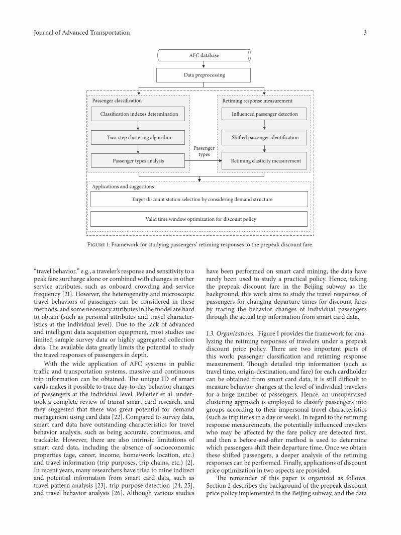
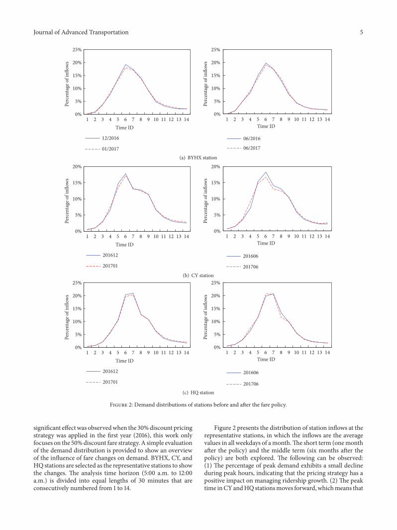
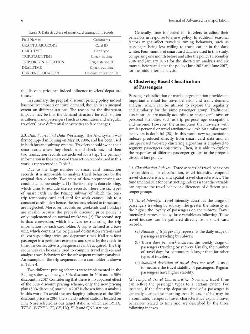
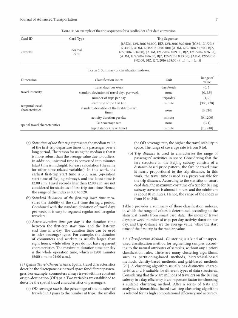
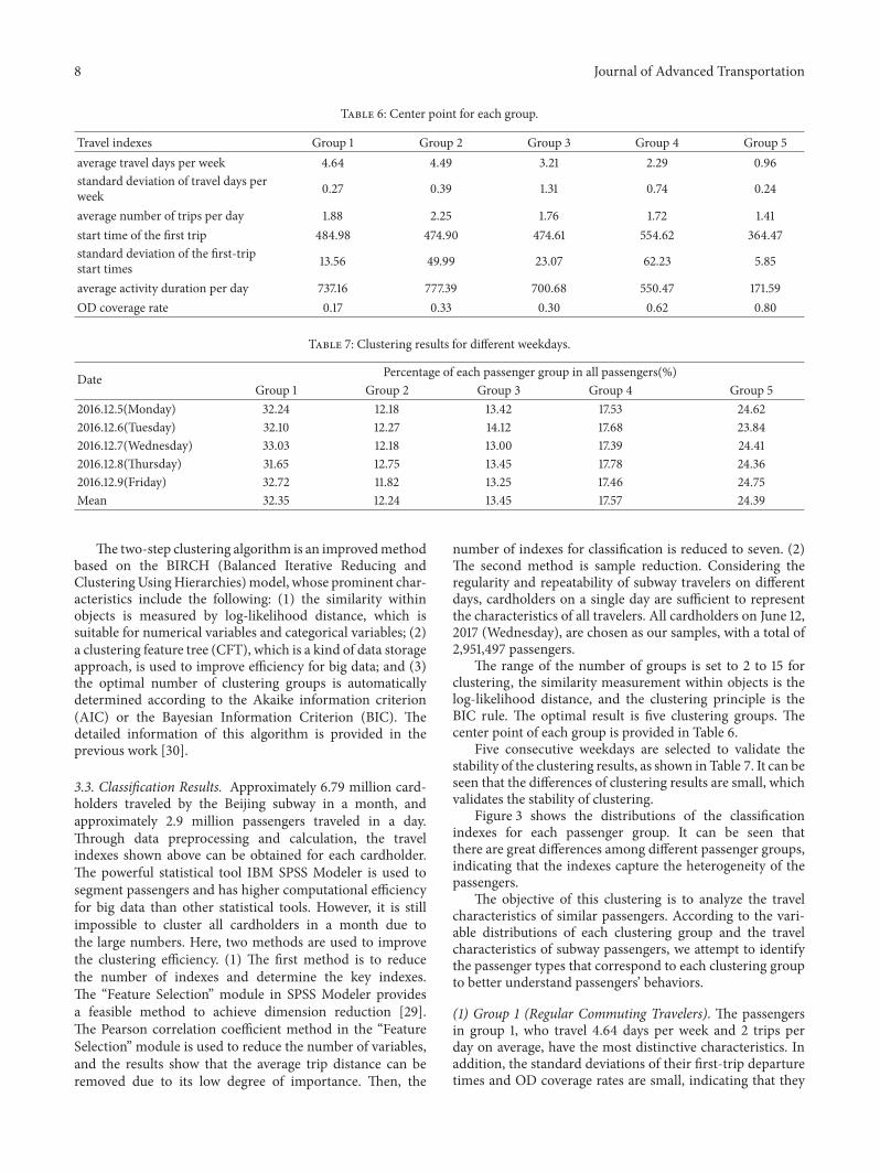
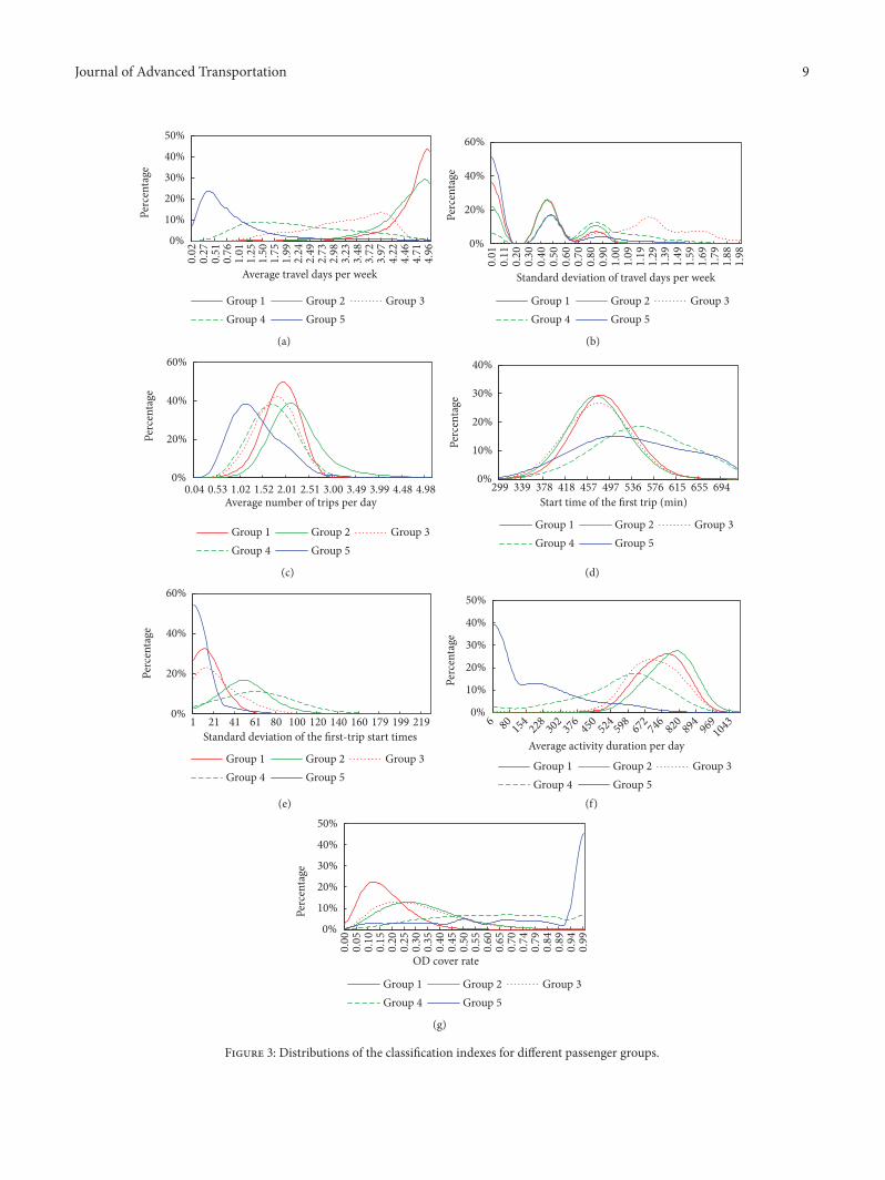
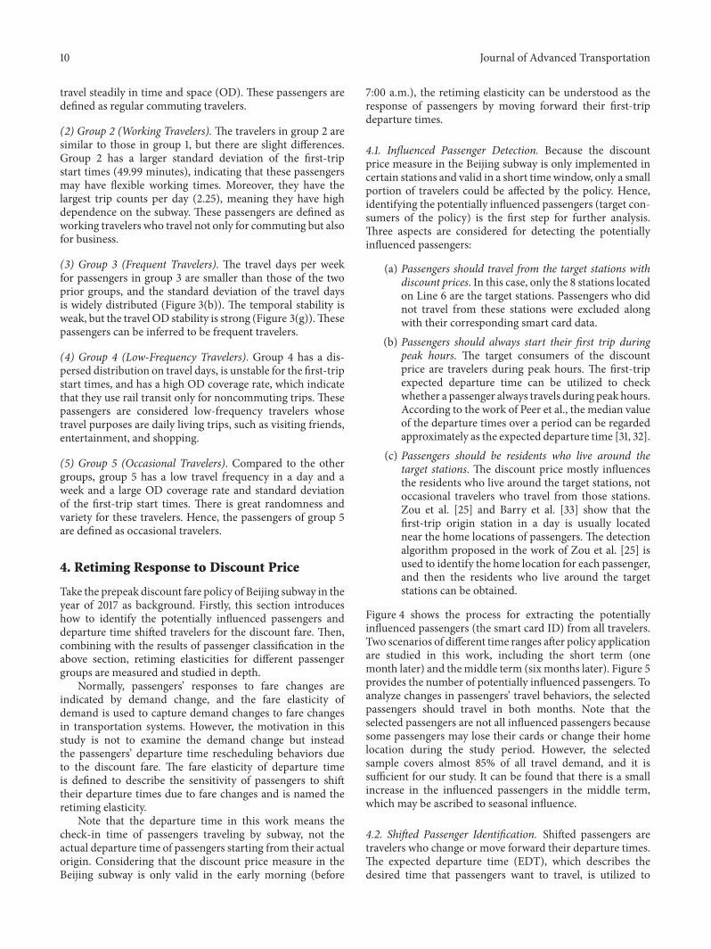
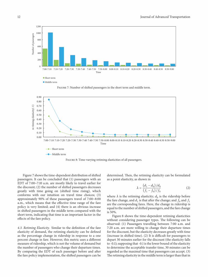
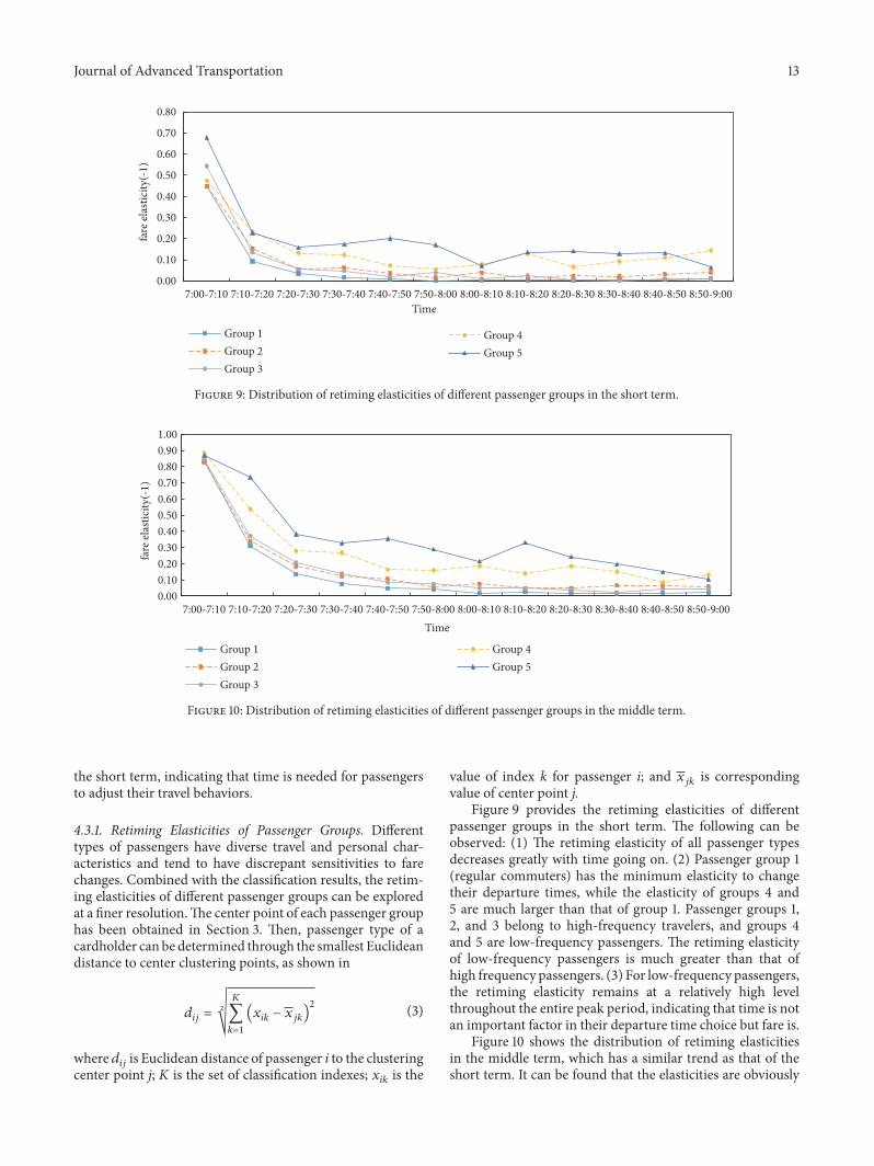
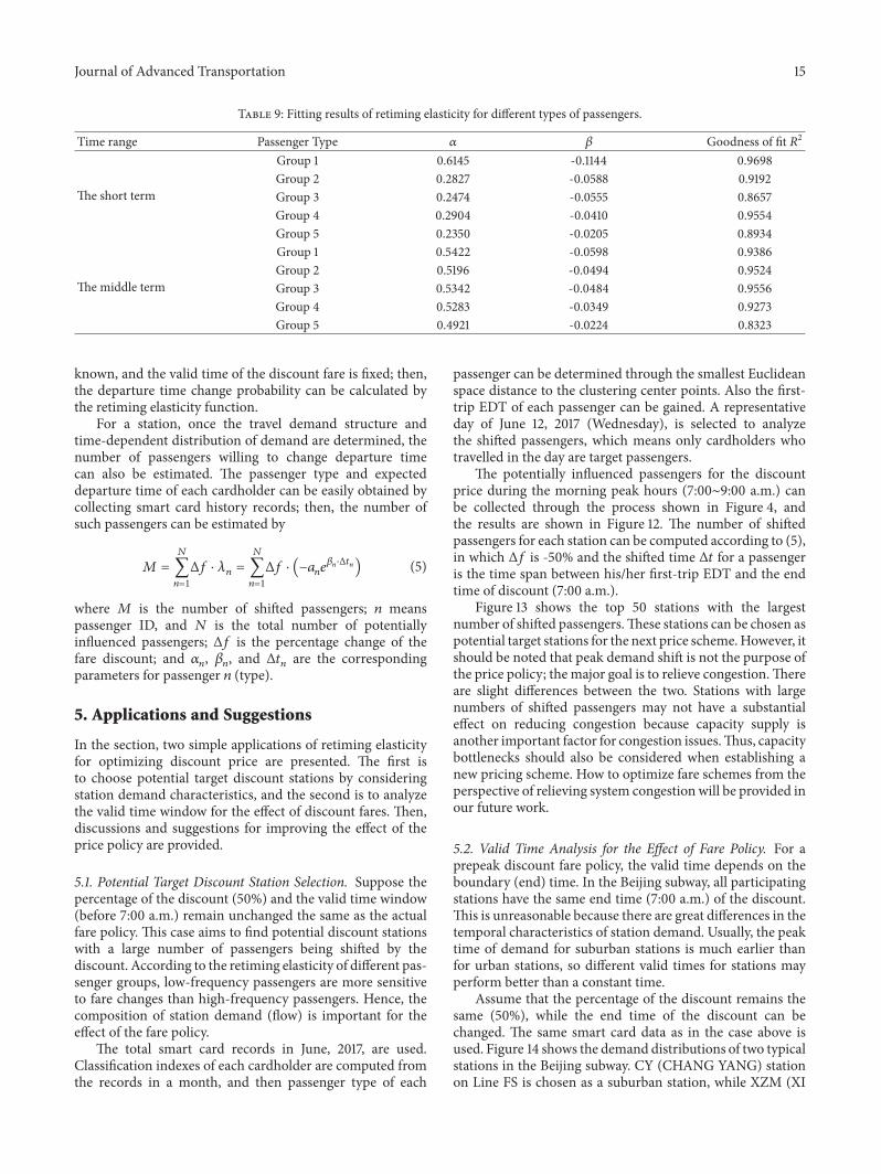
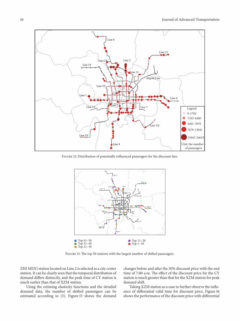

International Journal of
AerospaceEngineeringHindawiwwwhindawicom Volume 2018
RoboticsJournal of
Hindawiwwwhindawicom Volume 2018
Hindawiwwwhindawicom Volume 2018
Active and Passive Electronic Components
VLSI Design
Hindawiwwwhindawicom Volume 2018
Hindawiwwwhindawicom Volume 2018
Shock and Vibration
Hindawiwwwhindawicom Volume 2018
Civil EngineeringAdvances in
Acoustics and VibrationAdvances in
Hindawiwwwhindawicom Volume 2018
Hindawiwwwhindawicom Volume 2018
Electrical and Computer Engineering
Journal of
Advances inOptoElectronics
Hindawiwwwhindawicom
Volume 2018
Hindawi Publishing Corporation httpwwwhindawicom Volume 2013Hindawiwwwhindawicom
The Scientific World Journal
Volume 2018
Control Scienceand Engineering
Journal of
Hindawiwwwhindawicom Volume 2018
Hindawiwwwhindawicom
Journal ofEngineeringVolume 2018
SensorsJournal of
Hindawiwwwhindawicom Volume 2018
International Journal of
RotatingMachinery
Hindawiwwwhindawicom Volume 2018
Modelling ampSimulationin EngineeringHindawiwwwhindawicom Volume 2018
Hindawiwwwhindawicom Volume 2018
Chemical EngineeringInternational Journal of Antennas and
Propagation
International Journal of
Hindawiwwwhindawicom Volume 2018
Hindawiwwwhindawicom Volume 2018
Navigation and Observation
International Journal of
Hindawi
wwwhindawicom Volume 2018
Advances in
Multimedia
Submit your manuscripts atwwwhindawicom