Demand Based Signal Retiming Phase 2 – Real-World Implementation

Contract #: BDV27 TWO 977-01

Final Report

December, 2015

ii

Disclaimer

The opinions, findings, and conclusions expressed in this publication are those of the authors and not necessarily those of the State of Florida Department of Transportation.

iii

Metric Conversion Table

*SI is the symbol for the International System of Units. Appropriate rounding should be made to comply with Section 4 of ASTM E380. (Revised March 2003)

iv

Technical Report Page

1. Report No.

2. Government Accession No.

3. Recipient's Catalog No.

4. Title and Subtitle Demand Based Signal Retiming Phase 2 – Real-World Implemenation

5. Report Date November 2, 2015 6.Performing Organization Code

7. Author(s) Aleksandar Stevanovic, Jaehyun So, Marija Ostojic, Bratislav Ostojic, Natasa Petrovska, Deepti Pappusetty, Danilo Radivojevic.

8.Performing Organization Report No.

9. Performing Organization Name and Address Florida Atlantic University (FAU) 777 Glades Rd., Bldg. 36, Boca Raton, FL 33431.

10. Work Unit No. (TRAIS) 11. Contract or Grant No.

BDV27 TWO 977-01

12. Sponsoring Agency Name and Address Florida Department of Transportation (FDOT) Research Center 605 Suwannee Street MS-30 Tallahassee, FL 32399-0450 USA

13. Type of Report and Period Covered Draft Final Report 14. Sponsoring Agency Code

15. Supplementary Notes 16. Abstract Monitoring and managing arterial operations represents a significant problem for many public agencies in the US. Arterial streets, more numerous and covering much larger road networks than freeways, get less attention when it comes to deployment of ITS technologies and availability of data that is accurate and reliable enough to manage traffic in real time. Even when such data are available, the agencies face lack of developed procedures and strategies on how to handle such data in order to better monitor and manage arterial operations. The overall goal of this research was to develop a set of strategies for monitoring and managing arterial streets that would take in consideration idiosyncratic needs, challenges and policies of the public agencies managing arterials in southeastern Florida. Restrained by lack of resources and time, these agencies (Palm Beach County, Broward County, and City of Boca Raton) could benefit from FDOT and FAU assistance to improve their arterial operations. Thus the research presented here describes development of several methods and applications, which all heavily relay on various levels of available data, to monitor and manage traffic operations on arterial networks. Considering that ‘one-size-fits-all’ solution does not apply in real-life problems of Traffic Management Centers, the proposed techniques and applications cover a variety of field conditions and data specifications and thus they can be applicable to many other agencies in FL and nationwide. 17. Key Word Traffic operations, signals, monitoring, performance measures

18. Distribution Statement No restrictions.

19. Security Classif. (of this report)

Unclassified.

20. Security Classif. (of this page)

Unclassified.

21. No. of Pages

22. Price

v

Acknowledgements

The Florida Atlantic University research team acknowledges help and support from staff of the Traffic Management Centers in Broward County, Palm Beach County, and the City of Boca Raton. We also appreciate significant contributions from our team partners from Albeck Gerken Inc. and C2S Engineering Inc. and invaluable advices from the Project Manager and other FDOT District 4 staff.

vi

Executive Summary

Monitoring and managing arterial operations represents a significant problem for many public agencies in the US. Arterial streets, more numerous and covering much larger road networks than freeways, get less attention when it comes to deployment of Intelligent Transportation System (ITS) technologies and availability of data that is accurate and reliable enough to manage traffic in real time. Even when such data are available, the agencies face lack of developed procedures and strategies on how to handle such data in order to better monitor and manage arterial operations. The overall goal of this research was to develop a set of strategies for monitoring and managing arterial streets that would take in consideration idiosyncratic needs, challenges and policies of the public agencies managing arterials in southeastern Florida. Restrained by lack of resources and time, these agencies (Palm Beach County, Broward County, and City of Boca Raton) could benefit from FDOT and FAU assistance to improve their arterial operations. Thus the research presented here describes development of several methods and applications, which all heavily relay on various levels of available data, to monitor and manage traffic operations on arterial networks. Considering that ‘one-size-fits-all’ solution does not apply in real-life problems of Traffic Management Centers, the proposed techniques and applications cover a variety of field conditions and data specifications and thus they can be applicable to many other agencies in Florida and nationwide. Method to estimate signal performance measures based on link travel times – the purpose of this method was to enable use of commonly available point-to-point travel times to estimate performance of traffic signals. The objective of this method was to investigate if intersection-to-intersection travel times can be used to estimate performance of traffic signals. The method was proven to be very successful. The FAU researchers were able to estimate a signal’s through movement V/C ratio, Level of Service, and number of cycles necessary to pass through the signal; all based on link travel times. However, the major problem with this approach is availability of data. The method works well only after significant validation efforts and in the ITS-data-rich environment, (e.g. where video feeds are available from CCTV cameras and travel time measurement devices are located at each intersection). Future reduction in the costs of the ITS technologies and/or wider availability of high-precision travel time data from web applications may increase practicality of this concept. Regarding findings from the development of this method, the FAU research team recommends that future deployments of ITS/ATMS equipment are executed in such a way to comprehensively cover smaller spatial areas instead of stretching the ITS infrastructure over larger areas. A few devices sparsely located over larger area do not provide enough data to accurately and reliably estimate state of traffic conditions. Instead, FDOT decision makers should identify corridors/subnetworks with high priority, equip them with ITS infrastructure to properly monitor and manage traffic conditions and continue with next corridor/subnetwork once further equipment becomes available. This particular method requires travel time measuring devices at each signalized intersection and video detection that can recognize length of the queues and can be used to measure stop-line saturation flow rates.

vii

Method to evaluate the quality of signal timings based on traffic volumes from the field – objective of this method was to assist operators in evaluation of the currently deployed signal timing plans with regard to the fluctuation of the traffic flows recorded by the Microwave Vehicle Detection System (MVDS) detectors. A library of plans was developed and integrated in the spreadsheet that is able to recognize which signal timing plan is the best for the set of traffic volumes which are the closest to the MVDS volumes retrieved from the field. Theoretical practicality of this method is great because it can indicate benefits (% of performance index) if a different/better plan is selected. However, applicability of this method/tool again depends on availability of ITS data, which in this case represent multiple MVDS system detectors on a corridor. Another issue might be trust in the results obtained from deterministic signal optimization tool in the office/lab environment. Real-world traffic conditions have proven many times that solutions from the office do not always work effectively in the field. Recommendation related to this method is to install developed Excel spreadsheet and run its automatic routine based on traffic flows from MVDSs. Once the operators provide enough feedback about functionalities and reasonableness of this tool it can be improved to help operators identify quality of signal timings which are run in the field conditions. Testing of field traffic control strategies in simulation environment - this approach was aimed at establishing a reliable simulation model capable of replicating a variety of field traffic conditions. Its purpose was to enable TMC’s engineers and operators to monitor and/or test different signal timing strategies and conditions inside the simulation environment. The results of these efforts have shown significant improvement over running existing signal timing plans when working under a variety of nonrecurring and recurring traffic event scenarios. The biggest issue that we encountered in this task is that exercises that we performed in the lab cannot easily reflect field conditions. The major issue was replication of the ATMS.now performance, and all of its advanced features, in simulation environment. While this method still holds a lot of promises for the future, its full implementation would require availability of ATMS.now as a Software in the Loop (SIL) platform and potentially development of a connection between microsimulation system and a real-time feed from field data (MVDSs and travel time readers). FAU research team recommends that FDOT TMC operator review the way they report incidents and other events in the SunGuide system. It seems that information about length and extent of the incidents would be helpful to completely understand impact of such traffic events. There should be a method to minimize subjectivity of the traffic operators when rating the existence of intense traffic. It seems that word congestion (or oversaturation) is too loosely defined and there is no information to identify what is causing congestion, how far it reaches, etc. Also, one should consider a way to measure level of errors in the data logs and how these errors correlate to the workload issues and recording of data. Validation of the traffic management strategies in simulation - the main objective of this approach was to determine effective strategies for managing different sources of traffic congestion i.e. different types of traffic events by evaluating current TMC congestion mitigation strategies inside the simulation environment. The goal was to attempt to propose

viii

new signal control strategies that might prove efficient in dealing with impacts of most frequently occurring traffic events. Validation of the simulated traffic management strategies was constrained by the FAU team’s ability to replicate field conditions both on traffic side (making sure that simulation replicates field measurements) and traffic control side (use the same platform for ad-hoc changes in signal timings to respond to the traffic events). The results have shown that a decent match, between simulated and field data, was obtained for conditions where overall traffic demand did not deviate too much from the base conditions. For the other cases, it seemed that traffic conditions were so different that our base model did not make a lot of sense. This method still holds a lot of promises for future but its successful implementation will require a higher level of cooperation with third-party vendors, which was outside the scope of this project. The main recommendation for this activity is that FDOT invest in research to find out which of the existing signal-simulation interfaces would be the best to use to investigate impact of operators’ (signal timing) strategies on traffic conditions. This can be achieved through a highly-calibrated simulation study where operator’s signal actions can be performed as the simulation runs. Current ATMS.now setup limits options to model exact field signal timings in simulation environment. Application to assess level of traffic congestion based on Google traffic maps - purpose of this application is to enable traffic operators, at the agencies with limited (or no) ITS data, to monitor and assess level of congestion on the networks under their jurisdiction. The program captures color of color-coded links on Google maps to estimate percentage of congestion on the network of user’s choice. For larger regions/networks the program cycles through several smaller subnetworks to provide an overall network congestion assessment. The downside of this program is that it is not exact (difficult to draw links very accurately), and it depends on third-party support, implicitly. However, this tool still represents the key unique feature of this research and it is currently being tested at the Palm Beach County TMC. It is recommended that this method is further investigated and applied in field-like environment on continual basis to gather feedback from the operators and improve this tool. The tool should be redesigned to be compatible with FDOT database platforms to enable creation of various queries and customized reports and trend analysis of the performance metrics. Also, there is need to investigate potential of this tool for estimation of the impact of traffic signal strategies in a manner of before/after studies and its interfaces with other traffic data platforms, such as SunGuide/ATMS data, WAZE, etc. Visualization of the traffic incidents from SunGuide-like incident database - purpose of this activity was to use visualization of the incident records, stored in a SunGuide-like database developed for Palm Beach County, to identify ‘hot-spots’ in traffic operations (i.e., places where many incidents occur) and apply some strategies accordingly. Development of the tool was a success and the tool exhibited all of the intended features. Although there is a potential for future improvement, future implementation will depend on the decision of Palm Beach County and other agencies to use the same, SunGuide-like, database in future.

ix

The FAU research team recommends that this SunGuide-like incident database is further improved and provided to agencies around Florida, which do not have access to SunGuide but have a need for similar tool to visualize traffic and incident data. Further markers and legends can be added to make further cross-references between incident spots and locations of other traffic-related features. In overall, it can be concluded that this research project went more into width (than depth) of the objective to propose, develop, and test various methods and applications to assist traffic operators of various agencies in Southeast Florida to monitor and manage arterial operations. Variety and the quality of the tools developed, for a number of idiosyncratic requests and positions, document the seriousness of the faced problems and the needs for continuous work on improvement of the existing tools and development of the new ones. In order to find more about these methods and tools, and to make a request to download applicable tools, files and user manuals please contact Dr. Aleksandar Stevanovic at astevano@fau.edu or on the phone (561) 297-3743.

x

Table of Contents

1  Introduction ......................................................................................................................... 17 

1.1  Background .................................................................................................................... 17 

1.2  Objectives ....................................................................................................................... 17 

1.3  Study Scope .................................................................................................................... 18 

1.4  Summary of Project Tasks ............................................................................................. 18 

1.5  Document Organization ................................................................................................. 19 

2  Literature Review ............................................................................................................... 20 

2.1  Review of the relevant state-of-the-art ITS Technologies ............................................. 20 

2.1.1  Acyclica (analyzer software) .................................................................................. 20 

2.1.2  Sensys networks ...................................................................................................... 21 

2.1.3  3M LPRS ................................................................................................................ 22 

2.1.4  Connected Signals (formerly known as GreenDriver) - EnLightenTM ................. 22 

2.1.5  MetroTech net ......................................................................................................... 22 

2.1.6  Automatic number plate recognition system .......................................................... 23 

2.1.7  Q Vision system ...................................................................................................... 24 

2.2  Review of the research on Volume-Delay functions ..................................................... 25 

2.3  Summary of the literature review ................................................................................... 28 

3  Field Data Collection .......................................................................................................... 29 

3.1  Glades Rd Data Collection ............................................................................................. 29 

3.2  Broward Blvd Data Collection ....................................................................................... 30 

4  Methods for ITS-data-rich Traffic Management Centers .............................................. 35 

4.1  Estimating Signal Performance based on Link Travel Times ........................................ 35 

4.1.1  Required ITS technologies ...................................................................................... 36 

4.1.2  Methodology to estimate signal performance based on link travel times ............... 37 

4.1.3  Application of the travel-time-based signal performance measures ....................... 51 

4.2  Refinement of Signal Timing Plans for Broward Blvd based on Available ITS Data ... 56 

4.2.1  Reasoning for refinement of signal timing plans .................................................... 56 

4.2.2  Generalized overview of the method applied to refine signal timing plans ........... 57 

4.2.3  Definition of the break points for signal timing plans ............................................ 63 

4.2.4  Consideration of weekday TOD peak hour demands ............................................. 66 

4.2.5  Selection of the best signal timings based on field traffic volumes ........................ 67 

4.2.6  Application of the method in MS Excel auto-spreadsheet ...................................... 71 

4.3  Testing of TMC Strategies for Recurring and Nonrecurring Traffic Conditions .......... 76 

xi

4.3.1  Background ............................................................................................................. 76 

4.4  Validation of the Simulated Traffic Management Center Strategies ............................. 85 

4.4.1  Background ............................................................................................................. 85 

4.4.2  VISSIM model validation (new ITS data) .............................................................. 86 

4.4.3  Traffic event scenarios ............................................................................................ 89 

4.4.4  Methodology ........................................................................................................... 91 

4.4.5  General approach .................................................................................................... 92 

4.4.6  Scenario-Based Analysis ........................................................................................ 96 

5  Methods for Traffic Management Centers with Limited ITS Data ............................. 100 

5.1  Traffic Congestion Analysis Application ..................................................................... 100 

5.1.1  Application development ...................................................................................... 100 

5.1.2  Final application and instructions for users .......................................................... 103 

5.2  Visualization of Traffic Incidents based on SunGuide-like Incident Database ........... 113 

5.2.1  Background and task description .......................................................................... 113 

5.2.2  Development and characteristics of the application ............................................. 114 

5.2.3  User guide for the Incident Management System ................................................. 116 

5.2.4  Technical requirements ......................................................................................... 119 

5.3  Triggering Mechanisms to Assist Traffic Management Center Operators .................. 121 

6  Conclusions ........................................................................................................................ 124 

6.1  Estimating Signal Performance based on Link Travel Times ...................................... 124 

6.2  Refinement of Signal Timing Plans based on Available ITS Data .............................. 124 

6.3  Testing of TMC Strategies for Recurring and Nonrecurring Traffic Conditions ........ 125 

6.4  Validation of the Simulated Traffic Management Center Strategies ........................... 126 

6.5  Traffic Congestion Analysis Application ..................................................................... 126 

6.6  Visualization of Traffic Incidents based on SunGuide-like Incident Database ........... 127 

7  References .......................................................................................................................... 128 

xii

List of Figures

Figure 1. ITS on Glades Rd and the data collection sections ....................................................... 30 Figure 2. Broward Blvd. corridor with data collection devices placed along ............................. 31 Figure 3. ITS technologies used for data collection on Glades Rd .............................................. 37 Figure 4. General approach to monitor signals based on link travel times ................................. 38 Figure 5. MATLAB curve fitting flowchart ................................................................................... 43 Figure 6. SENSYS occupancy rate (Airport Rd – EB) .................................................................. 44 Figure 7. Free-flow travel time distribution (Airport Rd – EB) ................................................... 45 Figure 8. Saturation flow rate distribution (Airport Rd – EB) ..................................................... 46 Figure 9. Relationships between V/C ratios and link travel times ............................................... 48 Figure 10. VDF fitting curves (Airport Rd – EB) ......................................................................... 49 Figure 11. Validation Plot for BPR and new Volume-Delay functions ........................................ 50 Figure 12. User interface for program to calculate VDF measures ............................................ 53 Figure 13. Graphical representation of VDF measures on Google Maps ................................... 54 Figure 14. Visualization of VDF measures for northbound and southbound directions only ...... 55 Figure 15. Visualization of VDF measures for all directions of the selection ............................. 56 Figure 16. General approach used to develop new signal timing plans ...................................... 59 Figure 17. Flowchart of the actions taken to execute analysis of signal timing plans ................. 61 Figure 18. Location of MVDS midblock detectors along Broward Blvd. ..................................... 63 Figure 19. Location of Portable Traffic Monitoring Sites along Broward Blvd. ......................... 63 Figure 20. Relationship between current MVDS volumes and cycle lengths – Zone1 ................. 65 Figure 21. Relationship between current MVDS volumes and cycle lengths - Zone2 .................. 66 Figure 22. Excel-based traffic flow balancing tool ...................................................................... 68 Figure 23. Percent of improvement vs percent of total number of plans improved overall ......... 71 Figure 24. MVDS traffic data for every day and time interval ..................................................... 72 Figure 25. MVDS values displayed after filtering ........................................................................ 73 Figure 26. Calculate sheet with reference column ....................................................................... 74 Figure 27. Macro to identify the best matching volumes .............................................................. 75 Figure 28. Best suitable STP as a result ....................................................................................... 76 Figure 29. Data Smoothing Results using Travel Time and Estimated V/C ................................. 77 Figure 30. Traffic Detection Matrix ............................................................................................. 78 Figure 31. Changes in ATMS.now Signal Timings due to Increase in Traffic Demand............... 79 Figure 32. Volume and speed from a single detector during an incident ..................................... 80 Figure 33. Travel time and occupancy from a single detector during an incident ...................... 81 Figure 34. Traffic detection matrix for event traffic ..................................................................... 82 Figure 35. Example of traffic incident signature plot – July 9th, 2014 ......................................... 83 Figure 36. Example of traffic incident signature comparison plot – July 9th, 2014 ..................... 84 Figure 37. Example of traffic incident signature plot – September 12th, 2014 ............................. 85 Figure 38. Example of traffic congestion signature comparison plot – September 12th, 2014 .... 86 Figure 39. Model Validation Results – August data ..................................................................... 87 Figure 40. Early stage validation progress .................................................................................. 88 Figure 41. Broward Blvd traffic volume check ............................................................................. 89 Figure 42. Travel time validation (GPS vs VISSIM) for EB a) and WB b) directions ................. 90 Figure 43. Travel time validation (Bluetooth vs VISSIM) for EB a) and WB b) direction ........... 91 Figure 44. Saturated and oversaturated scenarios scope in the simulation model ...................... 94 Figure 45. Saturated and oversaturated scenario location .......................................................... 94 

xiii

Figure 46. Arterial incident scenario location ............................................................................. 95 Figure 47. Arterial incident scenario in the simulation model ..................................................... 96 Figure 48. Saturation and oversaturation detection strategy ....................................................... 99 Figure 49. Individual link performance is observable in the display ......................................... 101 Figure 50. Traffic Congestion Analysis Application .................................................................. 102 Figure 51. Congestion warning module ..................................................................................... 102 Figure 52. Interface of Traffic Congestion Analysis Application ............................................... 103 Figure 53. Files in the application package ............................................................................. 104 Figure 54. Main menu opens on second screen if exist .............................................................. 104 Figure 55. Main Menu Window .................................................................................................. 104 Figure 56. Create new subnetwork ............................................................................................. 105 Figure 57. Link monitoring window after clicking “Create New Subnetwork” on main menu . 105 Figure 58. Coordinates of the chosen center and zoom are displayed above the map .............. 106 Figure 59. Load existing subnetwork.......................................................................................... 106 Figure 60. Select Map window ................................................................................................... 107 Figure 61. Link monitoring window for the chosen map from “Select Map” window .............. 107 Figure 62. Operations with links on Link Monitoring window .................................................. 108 Figure 63. Clicking on the button to start capturing congestion metrics ................................... 108 Figure 64. Congestion metrics on the right side of Link Monitoring window ............................ 109 Figure 65. Warning message when threshold is not set ............................................................. 109 Figure 66. Capturing congestion levels and displaying results in side panel. ........................... 110 Figure 67. Output files generated in folder maps ....................................................................... 110 Figure 68. Functionality of “Run Configuration” button .......................................................... 111 Figure 69. Tabular output by the process to show the results .................................................... 112 Figure 70. Screenshot of log files ............................................................................................... 112 Figure 71. Configuration file example ........................................................................................ 113 Figure 72. Initial Design of Incident Record Management System ............................................ 114 Figure 73. Initial Design of Incident Record Management System ............................................ 115 Figure 74. Interface of the Incident Record Management System .............................................. 115 Figure 75. Graphical User Interface for the Incidents Management System ............................. 116 Figure 76. Selecting an incident by ID ....................................................................................... 118 Figure 77. Info box contents for the selected traffic event ......................................................... 119 Figure 78. Filtering by date and time simultaneously ................................................................ 120 Figure 79. Filtering by time frame when the incident happened and ended .............................. 120 Figure 80. The text file in .csv format representing the filtering for the chosen time frame ...... 120 Figure 81. The ID of the incident is the same as in the text file in .csv format .......................... 121 Figure 82. The intersection name is added in the tabular visualization of the incidents ........... 121 Figure 83. Traffic Strategies Triggering Procedure................................................................... 122 

xiv

List of Tables

Table 1. Traffic volume distribution per day per 15 minutes (M17 WB September 2014) ........... 31 Table 2. Traffic volume distribution per MVDS over 4- month period ........................................ 32 Table 3. Traffic volume distribution per each observed month (for all MVDSs) ......................... 32 Table 4. September 2014 traffic volume distribution per hour (MVDS M21 Westbound) ........... 33 Table 5. September 2014 traffic volume distribution per hour (MVDS M21 Eastbound) ............ 34 Table 6. Descriptive statistics of the data collected on Glades Rd ............................................... 47 Table 7. Data format requirements for program to calculate VDF measures ............................. 52 Table 8. Meaning of the differences between various performance indices ................................. 59 Table 9. Example of MOEs for Broward Blvd. for September 8, 2014 ........................................ 60 Table 10. Traffic counts from various sources ............................................................................. 64 Table 11. Current STP vs Optimal STP - example scenario evaluation for September 8, 2014 .. 69 Table 12. Relative difference in traffic volumes “design” vs. “balanced” .................................. 70 Table 13. Arterial Incident Sub-Scenarios.................................................................................... 96 Table 14. Summary of considered scenarios ................................................................................ 97 Table 15. Signal timing pattern for the Base Scenario ................................................................. 98 Table 16. Relationship between Traffic Condition and Road Segment Color ............................ 101 Table 17. Data format requirements ........................................................................................... 117 

xv

List of Selected Acronyms and Abbreviations

AADT Annual Average Daily Traffic ANOVA Analysis of Variance ATCS Adaptive Traffic Control System ATIS Advanced Traffic Information System ATMS Advanced Traffic Management System AVI Automatic Vehicle Identification BCTED Broward County Traffic Engineering Department BlueTOAD BlueTooth Travel Time Origination And Destination CBD Central Business District CCTV Closed Circuit TV CFEM Curve-Fitting Estimation Model CMS Changeable Message Signs CTAC Combined Traffic Assignment and Control DBSR Demand Based Signal Retiming DMS Dynamic Message Signs DOS Disk Operating System DSS Decision Support System DTA Dynamic Traffic Assignment FAU Florida Atlantic University FDOT Florida Department of Transportation FEC Florida East Coast FEFM Federated Evidence Fusion Model FHWA Federal Highway Administration GA Genetic Algorithm GIS Geographic Information System GPS Global Positioning System GUI Graphic User Interface ICM Integrated Corridor Management ITS Intelligent Transportation System LTSO Left Turn Spillover MAPE Mean Absolute Percentage Error MILS Man-In-the-Loop Systems MOE Measure Of Effectiveness MPO Metropolitan Planning Organization MVDS NBA

Microwave Vehicle Detection System National Basketball Association

O-D Origin-Destination OIL Operator in the Loop PTV Planung Transport Verkehr

xvi

RBC Ring Barrier Controllers RCP Recursive Cell Processing RT/IMPOST Real-time Traffic Control Policy RTOR Right Turn on Red SCATS Sydney Coordinated Adaptive Traffic System SCOOT Split Cycle Offset Optimization Technique SDOT Seattle Department of Transportation SIL Software in the Loop TDM Travel Demand Models TMC Traffic Message Channel TOD Time of the Day TRPS Traffic Responsive Pattern Selection TSM&O Transportation Systems Management and Operations UTDF Universal Traffic Data Format VB.NET Visual Basic .NET VDS Video Detection Systems VISGAOST VISSIM Based Genetic Algorithm Optimization of the Signal Retiming VMS Variable Message Signs VNP Virtual Next Phase

17

1 INTRODUCTION

1.1 Background

The objective of the Demand-based Signal Retiming (DBSR) Phase 1 research was to develop methods that can be implemented by a signal maintaining agency in Florida to measure and report demand in real-time and to predict demand using microsimulation models. The research presented in this report is a continuation of the DBSR Phase 1, but its main purpose was to implement the findings and methods of the DBSR Phase 1 by using available ATMS data. High fidelity traffic simulation models were developed in VISSIM microsimulation platform and used for multiple purposes in this study including modeling traffic demand from the available data sources. Also, multiple recurring and nonrecurring congestion scenarios were developed and appropriate strategies were defined to alleviate the congestion of different traffic scenarios. The outcome of Phase 1 study included traffic operating guidelines, which can be used by traffic operators in Traffic Management Center (TMC). The objective of this research project (Demand-based Signal Retiming Phase 2) was to refine the research results from Demand-based Signal Retiming Phase 1 through field implementation of the proposed strategies and methods. As such, this research included different efforts to collect field data and develop various approaches which were demonstrated to FL DOT and other local agencies. Second phase of the study represents an extension (Phase 2) of the DBSR project whose primary objective is to implement methodologies and procedures developed in Phase 1 and to investigate applicability of proposed methodologies to areas not rich in ITS traffic data in order to better control and manage traffic congestion in Broward and Palm Beach Counties. West Palm Beach was selected as an excellent environment to extend the methodology developed in Phase 1. Unlike central Broward County, which is expected to benefit from many traffic data sensors recently deployed within the Advanced Traffic Management System, Palm Beach County can only rely, like many other places around the country, on basic traffic detection inputs, which usually include feeds from local detectors at signalized intersections and relatively new traffic information services from web applications (Google, Bing, INRIX, etc.).

1.2 Objectives

The following research objectives and tasks will be pursued in the Phase 2 of the project:

Refine signal timing plans and traffic demand prediction methods and procedures (developed in Phase 1 of the project) in the Traffic Management Center (TMC) environment for Broward County.

Extend the methodology developed under Phase 1, for traffic-data-rich environments such as Central Broward, to areas like West Palm Beach downtown where there is a common level of traffic sensors deployed in the field.

Investigate the feasibility of using existing data sources to develop a set of traffic indicators (e.g. congestion or travel time contour maps), which could be used by PBC TMC operators to effectively monitor traffic conditions in West Palm Beach network. The purpose of this task is to qualitatively assess management of available data to improve traffic operations without large investments.

18

1.3 Study Scope

The scope of the research includes City of Boca Raton, and Broward and Palm Beach counties. Specific research interests included Fort Lauderdale downtown area of Broward Blvd. This area is equipped with ITS infrastructure “ATMS Installation in Central Broward County Phase I (FM #427971-1)”. The project includes the design and deployment of ATMS infrastructure along portions of Broward Blvd., Sunrise Blvd., Oakland Park Blvd., US1/Federal Hwy, SR-7, and University Dr. The project components include 10 dynamic message signs, 63 traffic-monitoring cameras, 33 travel time collection sites, 54 vehicle data collection devices, software to manage the devices, and approximately 18 miles of fiber optic cable and required conduit. It should be noted that there are two more ongoing ATMS installation projects covering southern Broward County (Phase II) and three major corridors (Phase III). ATMS Installation in phase II of the project covers sections of Hallandale Beach Blvd., Hollywood/Pines Blvd., Pembroke Rd., and US-1/Federal Hwy, SR-7, University Dr., while project phase III will cover sections of US 441/SR-7, University Dr., and Griffin Rd. depicts the Transportation Systems Management & O network in Broward County. Multiple ATMS infrastructure installation projects have been planned in Palm Beach County and are intended to start during summer 2014. These projects will cover sections of Southern Blvd., Northlake Blvd., and Okeechobee Blvd.

1.4 Summary of Project Tasks

In order to achieve research objectives the following tasks are conducted. Each task is accompanied with a short description on which chapters of this report address each of the tasks.

Implementation of procedures and methods from Phase 1 in Traffic Management Center (TMC) operations – addressed through various chapter but the most of the text that addresses this task is located in chapters 4 and 5.

Collection of field traffic data from TMC – descriptions of the field data collections are scattered throughout the report but the summary is provided in chapter 3.

Refinements of strategies for recurring and nonrecurring events – almost exclusively described in chapter 4, although some of the activities described in chapter 5 are also relevant.

Conduct a literature review on the handling of traffic operations in congested networks – this task is almost entirely addressed in chapter 2.

Investigate how to report network traffic conditions from available data sources – this task is exclusively addressed by chapter 5.

Identify triggering mechanism that can assist/replace traffic operators – this task is addressed by various project activities, which is documented in various chapters (mostly 4 and 5) of the report.

Develop qualitative strategies to improve traffic operations based on existing data – this task is addressed by various chapters (mostly 2, 4 and 5) of the report.

19

1.5 Document Organization

This final report is presented in six chapters. The first chapter introduces the problem and motivation for this research. It also lays out background that led into the need for research as well as specific tasks which were supposed to be accomplished during the course of this study. The second chapter consists of a literature review on a number of subjects and it is divided in 3 subsections. The first subsection is related to the review of the existing technologies that are used to monitor arterial/signal performances. The second subsection provides review of the existing studies on volume-delay functions, and the third subsection summarizes findings from the previous two subsections from the perspective of importance and applicability of the reviewed studies for the research presented here. The third chapter covers the data collection of the traffic metrics from the field. Considering that various descriptions of the data collection are scattered throughout report to describe various activities, the authors wanted to provide a summary what was (and how) collected based on geographic scope of the two major data collection campaigns (Glades Rd and Broward Blvd). Chapters four and five represent the core of methods done under this research and they reflect the needs to address specific tasks, as expected by FDOT and other stakeholders. Chapter number four covers a number of activities and methods, which were developed for arterials rich with ITS data. The activities and application in this chapter cover a relatively wide range of topics, from estimation of the signal performance metrics based on link travel times, through development of methods to assess quality of signal timings and relevant changes based on the changes in traffic volumes, to development of scenarios and strategies to handle various recurring and nonrecurring traffic events. Chapter five, contrary to the previous chapter, covers development of methods for operators of those traffic management centers which do not have sufficient number of ITS sensors and devices to comprehensively cover their traffic network. Such methods and applications cover subjects from assessing congestion in the networks with no detectors in the field. Available third-party applications are used to gather information about state of traffic to the programs which convert simplistic tabular incident data into map-based databases with visual features. Chapter number six concludes this report by describing achievements and limitations of various activities and presenting recommendations for future research and implementation of the developed methods.

20

2 LITERATURE REVIEW

2.1 Review of the relevant state-of-the-art ITS Technologies

The FAU research team reviewed relevant academic papers and technical reports related to state-of-the-art ITS technologies. The ITS technologies reviewed are listed below with summarized information.

Acyclica (Analyzer Software) offers a tool for analyzing data (Acyclica, LPR and other Bluetooth scanning technologies) regarding TMC congestion mapping, Traffic Reporting and Origin-Destination Analysis.

Sensys Networks’ wireless vehicle detection solutions provide accurate, real-time data, intended for arterial/freeway performance measurements, traffic engineering analysis and traveler information.

3M LPRS license plate recognition (LPR) technology can be integrated into various systems for travel time and average speed management or electronic toll collection.

GreenDriver/EnLightenTM (now known as Connected Signals) is a mobile app with vehicle-to-infrastructure (V2I) functionality, which uses real-time traffic light data provided by other sources to calculate and present dedicated routes that avoid red lights.

MetroTech operates as a third party traffic data provider whose main objective is to aggregate presently available sensor, GPS and camera feeds (governmental infrastructure) and provide an integrated video and traffic analytics to clients in real time.

Automatic Number Plate Recognition System (ANPR) reads the plate number each time a vehicle passes each of these two locations. Plate number strings and time-stamped tags are sent via wireless connection to the central server. The server matches the plate number strings and time-stamped tags collected at different checkpoints in order to measure the travel time.

Queue vision is located in work zones where road and traffic conditions are different from regular conditions. The collected data are distributed to motorist in different ways, depending on the spatial location of the motorists the system intends to serve. Further applications of queue vision technologies include ability to live stream updates of current traffic conditions.

2.1.1 Acyclica (analyzer software)

Acylica’s web-based platform is a useful tool for congestion analysis. Acyclica’s software is able to process large number of data and as an output provides information with practical value. Information from this software can be used to assist agencies to retrieve travel times, traffic patterns and congestion. The software can be used with any standard web-browser. Analytics include route travel times by segment, route delay, speed, route speed by segment, timing plan analysis, day of week analysis, weekly analysis, delay by phase and approach, etc. As Analyzer's map interface Acyclica uses Google Maps, which provide a common interface. Acyclica is using multiple databases for data storage to ensure reliability and persistency of the data. Same databases are keeping data stored forever so users can always have access and extract their records of traffic information. By analyzing complex routes one segment at a time,

21

Acyclica Analyzer helps to identify congestion events and understand their greater impact. Selecting routes and comparing different day's data is relatively easy for users. This software also provides a way to visualize vehicular queues through queue estimation based on the strength of the received Wi-Fi signals. The central back-end provides a simple method for inter-agency data sharing (Acyclica Analyzer, 2014).

2.1.2 Sensys networks

Sensys Networks make wireless sensors and associated networking components to detect vehicles and monitor traffic. Sensys Networks has designated its wireless sensor protocol to meet the demanding system level requirements of their applications. The protocol and underlying implementation have proven to be robust and very effective. SensysTM Wireless Vehicle Detection System uses pavement-mounted magnetic sensors to detect presence and movement of vehicles. The sensors – installed on the surface or in small holes cored in the roadway – transmit detection data in real-time via low-power radio technology to a nearby Sensys Access Point. Vehicle detections are further relayed to a traffic signal controller, remote traffic management center or other systems. Typical Sensys sensor is a sensitive magnetometer equipped with a low-power radio, packaged in a small plastic case. Every Sensys system installation consists of:

A number of Sensys wireless sensors at various locations depending on particular application

Access point which is responsible for receiving, processing and further transmitting of the detection data

One or more Sensys repeaters needed depending on the radio range of the access point(s)

The most important part of every Sensys system is the access point since its role is to communicate the detection data received. Providing accurate vehicle detection at particular positions needed, allows Sensys Networks’ sensors to be implemented in a wide variety of applications. First and foremost, precise traffic data collection including vehicle counts, occupancy and speed, then traffic signal control data: stop bar detection, advance detection, dilemma zone protection and ramp management. One of the advantages of Sensys Networks’ wireless detection system is its ease of installation (one sensor in less than 10 minutes). No cabling or long saw cuts are required and the circular pavement hole produces the least damage to the roadway. Sensys has designed their sensors to be capable of mechanically sustaining pavement-mounted settings and operate over a temperature range from -40 to +85 degrees Celsius. SNAPS manager represents an integrated software application for managing Sensys Networks vehicle detection data. It provides statistical processing and remote network monitoring. Each access point is able to communicate the data from all its dedicated sensors via IP communications to a central server for data analysis and archiving. One of the main features of the SNAPS software is traffic data collection, archiving, and analysis - automatic data collection and archiving, detection data automatically processed providing per-vehicle or per-lane statistics, traffic analysis and network performance predefined and customized reports,

22

geographical representation of Sensys devices against topographical maps (Sensys Networks, 2011).

2.1.3 3M LPRS

3M's LPRS represents technology developed in a way to address industry need to have a variety of fixed and mobile ALPR systems for different applications. 3M fixed LPR cameras provide continuous monitoring of vehicles, communicating all database hits to agencies for deployment, and creating an evidentiary record of an infrared license plate image and color overview image of the vehicle. Company developed specific ALPR software, which is being used to solve a variety of road dilemmas including tolling enforcement and congestion charging, as well as unique applications like bus lane enforcement and traffic data collection. Technology developed by 3M, continuously searches the camera’s field of view for the presence of a license plate. A dual lens camera is triggered to capture a color image of the vehicle and an infrared image of the license plate. The robust BOSS back-office software enables users to organize and archive data generated by the fixed and mobile units for analysis, investigative support, and alert notifications (3M Co, 2014).

2.1.4 Connected Signals (formerly known as GreenDriver) - EnLightenTM

Green Driver, a startup company from Oregon, has partnered with traffic equipment manufacturer, Trafficware, in order to develop a smartphone application called ‘EnLighten’. Application communicates with central traffic management systems in order to provide drivers with predictions on how long they will be stopped at traffic lights. Trafficware has a very flexible and extensible central software system, which allows possible integration with third-party software products, such as the EnLighten app. Trafficware provides the real-time traffic signal data for intersections to Green Driver, creating opportunities for drivers to have a more relaxing and informed driving experience, as well as providing additional driver safety, fuel efficiency, and reduced emissions. In a survey that the company conducted, most of the feedback from users was positive and provided information reduced amount of stress and anxiety while waiting for signal to turn green. Having information about time until the next green, drivers that are distracted or engaged in other activities can have their attention back to the driving tasks before the light turns green. Trafficware provided in this application real-time data about the traffic signal that gives drivers a whole new level of insight into their driving experience (Connected Signals, 2015).

2.1.5 MetroTech net

MetroTech Partners was founded in 2007 with with main idea of developing Advanced Analytical Software for Intelligent Transportation Systems. MetroTech aggregates real-time traffic data from any video stream, applies analytics, and publishes actionable information.

The primary goal of the MetroTech is to provide ITS applications and services that deliver detailed traffic information to be used as probe data for ITS initiatives such as Integrated Corridor Management (ICM). MetroTech Net is able to provide broad and detailed information

23

which can be used for the purpose of applying techniques to mitigate congestions such as adaptive signal control, ramp metering, and adaptive pricing.

The foundation of the MetroTech Net is Networked IP Video Cameras coupled with hardware and software enhancements that together make these cameras very accurate sensors. With more capabilities and intent of conventional CCTV, and low bandwidth traffic cam pictures of congestion, MetroTech Net delivers real-time video that can be used to realize various ICM initiatives. The MetroTech Net offers automated traffic analysis, provides a complete picture of traffic conditions, rapidly recommends incident impact measures, and can provide predictive behavioral analytics to the advantage of the transportation authority. Technology provided by MetroTech Net presents complete system that works and provides more than previous video applications, like speed and flow detection on expressways, and fulfils the requirement for the higher-resolution imagery that complex analytics demand. These additional video analytics are able to provide alerts, record transportation events, and assist with long-term infrastructure and safety planning.

The basis of the concept proposed is the smart-camera wireless grid known as IntelliSection. IntelliSection essentially enables accessibility of the images, traffic information, and applications through cloud computing. Delivered from the cloud, traffic Big Data is analyzed and published via API’s to mobile or web applications. Collecting a repository of government infrastructure-based data is the IntelliSection™, which turns existing cameras into sensor data. It enables, in real-time, creation of virtual IntelliSections (intersections) with lane level accuracy, to constantly monitor and record the actual events and performance, not the estimated or projected conditions. Data generated is analyzed and offered as real-time, complete traffic information to public entities, corporations and other consumers via a variety of distribution channels (MetroTech Net, 2014).

2.1.6 Automatic number plate recognition system

Automatic Number Plate Recognition System (ANPR) systems generally require high quality cameras with fast frame rates to capture an image of the number plate with enough definition for the system to define the vehicle’s registration number. Such cameras are relatively costly to install and maintain. The latest developments in ANPR technology: a single sensor can measure and differentiate traffic in both directions, enable the simultaneous capture of up to four license plates while also detecting the direction of travel. Furthermore, the ANPR technology can measure journey times with a match rate currently unobtainable with Bluetooth/Wi-Fi tracking. Combined with classification technology, vehicles can be differentiated by class and their origin (for certain countries and regions). This is done as a matter of routine for tolling applications in some countries. Cameras can be independently time-locked using GPS time (primary) with a high stability crystal oscillator driven Real-time clock (secondary reference). This configuration is sufficiently accurate and reliable to be used in average speed enforcement systems to detect vehicles travelling up to 140mph. Key benefit of the ANPR Technology can be used simultaneously for both enforcement and civilian functions. These combined solutions can be a

24

good way to spread the cost of a system between, for example, a local authority and other organizations that may wish to share the ANPR data. The embedded camera technology typically includes two cameras within a single enclosure. One provides contextual images for color overview, while the other is dedicated to ANPR. It is possible to stream MJpeg over HTTP ‘video’ from either camera. While not optimized for CCTV streaming, the color overview camera could provide this functionality. Whilst the quality may not be as high as a dedicated CCTV system, the output may be adequate for viewing congestion, accidents and incidents. In the past ANPR systems have been sensitive to environmental conditions. The use of improved housings, often nitrogen purged and usually sealed to IP67, has overcome these problems and extended the operating temperature range between -40ºC and +60ºC (ARH Inc., 2014).

2.1.7 Q Vision system

Qvision Technology is a type of advanced video distribution service that takes advantage of the capabilities of today’s computing and advanced video distribution technologies. It provides near real-time looped moving images from traffic cameras that are updated at regular intervals. Qvision system was originally designed and intended for monitoring border crossings and the first one implemented in the world was the one at the border of Mexico and California, that can be considered as one of the world’s busiest border corridor. Travelers had no reliable way to check current conditions so they could make decisions about when to cross and which of the multiple approaches to use. The problem was serious because the border patrol had no way to see the ends of the lines in Mexico. Qvision technology was implemented by BorderTraffic.com website and it allowed users to observe almost real-time traffic conditions. As a result, now travelers can visit BorderTraffic.com and choose from 16 different views that cover all crossing access points, each with a live loop video clip that clearly shows the length and speed of that particular line. Some of the after-implementation findings showed up to 15-20% reduction in travel/delay time.

The main benefit of the Qvision system is its cost effectiveness, since it is allowing for almost real-time data to be available at any time at a cost of implementing still images. Cost savings over existing software and hardware solutions can be from 50 – 80%. Via computer or mobile device travelers receive updated videos that have all the benefits of live streaming without the cost and need for dedicated hardware. Qvision was designed to be adaptable and flexible in implementation. When considering fusion with existing DOT systems, Qvision is proven to be a valuable solution since it does not require extensive integration. In order to comply with the security standards and protect the information and the source, the software implemented allows for different security features to be designed and incorporated, based on particular requirements of the entity involved (customized protection feature). DOT’s have their own administration page which permits them to assign privileges and a number of security restrictions, this page is designed in order to protect DOT’s sharing information with other entities. The user then logs in through any browser on any device to access the permitted images. Qvision can capture, manage and display CCTV video received from any location via fiber optic, DSL, Ethernet-over-Copper and cellular communication links. Ability of the system to communicate via cell modem or long-range wireless systems is allowing the areas that have not been covered till now due to inability

25

to connect to the internet, to be served and monitored. Qvision system also provides real-time viewing and pan-tilt-zoom control, readily available for operations centers. Another benefit is the ease of sharing of real time streaming video with other agencies i.e. other transportation departments, police, EMT, fire, and others. This feature is enabled through a browser based video stream delivery. Traffic control centers very often utilize a sophisticated procedure in order for the operators to be able to observe the desired image from a CCTV camera. It is an automated process but it can require up to four servers and six application processes. Qvision is able to provide the same feature but in only four steps and through a single application.

The only issue is compatibility and if the cameras are compatible with Qvision software, then the IP address is all that is needed and live videos will be available on agencies’ website. Qvision interfaces with the cameras without any changes to traffic management’s center’s/agency’s current system and Qvision software can streamline command center operations. One of the advantages of this technology is that it allows connection to virtually any camera in the world. Qvision is providing an option to set up and program an entire website for the agency that requests its services. Qvision system allows a customer to choose the desired time between new video loops. In addition, the length of the loop can also be changed. When it comes to monitoring and using the video from remote locations where the cost of putting in a fixed line for a camera could be too high, Qvision offers additional benefits. Its software does not require a constant internet connection - only required equipment is camera, power (solar or line), and a cellular modem to monitor a route cost-effectively. (Qvision Technology, 2014).

2.2 Review of the research on Volume-Delay functions

Many studies have been conducted to develop the Volume-Delay Functions (VDFs) and calibrate the VDF parameters. The main purpose of VDFs is to assign traffic volumes over the road network by estimating the level of congestion (i.e., delay) at the macroscopic transportation network analysis level. Since the Bureau of Public Roads (BPR) function was developed (Bureau_of_Public_Roads, 1964), many different types of VDFs have been proposed and used in practice by deriving new functions or calibrating the VDF parameters. This section describes the efforts in developing and calibrating VDFs. Spiess (1990) proposed a Conical VDF to overcome the inherent drawback of BPR that the BPR-estimated delay is over-sensitive during V/C > 1.0 when a high value of alpha is used. The named ‘Conical’ was due to its geometrical representation as hyperbolic conical section of the plotted curve. The author examined the functionality of the Conical VDF though seven requirements for a well-behaved VDF. Akcelik (1991) proposed a new VDF based on the delay parameter consistent with the formula used for estimating intersection delays. This Akcelik’s VDF consists of minimum travel time (i.e., free-flow travel time), capacity, and delay parameters, and this study recommended that the delay parameters need to be determined by regression analysis using the specified minimum travel time and capacity values. Horowitz (1991) suggested the parameters for VDF in the purpose of enabling the travel forecasting methodology consistent with the Highway Capacity Manual (HCM) delay estimation methodology. This study implemented the travel time-volume relationship while travel time was derived from the HCM signalized intersection delay formula. As a result, the best BPR function

26

parameters were suggested as being α = 5.0 and β = 3.5. Kurth et al. (1996) compared the performances of HCM delay-based VDF and BPR function in terms of the congestion estimation on interrupted/uninterrupted flow. In this study, percent root mean squared errors for the HCM delay-based VDF and BPR were very close, but BPR was a good fit for uninterrupted flow (i.e., freeway) while the HCM delay-based VDF produced more accurate traffic volume and speed in the network. Li et al. (1996) investigated a delay model for signalized arterials considering near-saturated and over-saturated traffic conditions. This research indicated that the signal controller’s performance was the key element in modeling near-saturated or oversaturated networks. An overflow delay model for signalized arterials was proposed and calibrated from the database generated from the random queue model. An overflow delay expression was based on Akcelik’s VDF, since it showed that the presence of downstream queues had a strong influence on the performance of the system with the limited queuing space. The model was described as a good supplement for the current HCM models. Fambro and Rouphail (1997) also developed a generalized model for estimating delay based on HCM VDF. The model considered the actuated-control parameters, oversaturation and variable demand, and the parameters accounting for these signal and demand aspects were added to the HCM VDF. The model was proved to be a good predictor of delays by observing the field-collected delays and the simulated delays obtained from the microscopic traffic simulation model. Skabardonis and Dowling (1997) evaluated the performances of existing speed estimation techniques such as BPR and Akcelik VDF. This study proposed the speed-flow relationships adequate for different types of roads and a calibrated BPR curve with the suggested parameters’ ranges (i.e., α from 0 to 1.0 and β from 4 to 11) under the maximum capacity instead of using the practical capacity used in standard BPR. The new curve has been validated against speed-flow data obtained from uninterrupted and interrupted flow conditions, and the authors affirmed Akcelik’s function to be better suited for more detailed analysis (i.e. microscopic level). Dowling et al. (1998) also used BPR and Akcelik VDF for estimating link speeds. The travel time and traffic count data were collected by the floating car methodology on both freeway and arterial road segments during the morning peak period. Also, two macroscopic simulation models, FREeway Queue (FREQ) and TRAffic Network StudY (TRANSYT) were used to develop a hypothetical data set for testing the speed-flow curves against conditions in which demand exceeds capacity. As a result, an updated BPR curve overestimated the impact of congestion at high demand-to-capacity ratios, and it drops dramatically to zero as demand-to-capacity ratios exceed 1.00. Also, Akcelik VDF showed significantly higher accuracy for very high demand-to-capacity ratios, and it was more preferable in predicting the linear impact of congestion on speeds. By following the Dowling’s study, Singh and Dowling (2002) compared Akcelik to BPR, HCM VDF, and modified BPR travel time function on the freeways sections using the root-mean square error (RMSE). Akcelik’s function had the lowest RMSE value and BPR and the modified BPR followed. In later studies, attention was directed toward improving the existing VDFs, primarily BPR. Yun et al. (2005) proposed an updated delay estimation methodology for the use in urban travel demand forecasting. BPR’s standard speed-flow relationship was modified to include the impact

27

of truck traffic on freeway congestion by including an additional parameter. Based on the simulation results for urban arterials, the BPR curve was also modified by using specific coefficients accounting for different levels of signal control densities at signalized arterials and classified into four separated categories (i.e., α= 0.283 and β=3.018 and ɣ=2.249 for freeway operations and range from 0.074 to 0.136 for α, 1.105 to 3. 140 for β and 5.058 to 21.281 for ɣ for arterials). Dowling and Skabardonis (2006) examined the performance of the most commonly used VDFs (i.e., linear, logarithmic, exponential, power, polynomial, BPR, and Akcelik) in the purpose of investigating whether or not the conventional VDFs meet the requirements for a well behaved VDF defined by Spiess (1990). Three volume delay functions (BRP, Akcelilk and Exponential) were proven to satisfy the Spiess’s requirements while the others (i.e., linear, logarithmic, power, and polynomial) did not. Xiong and Davis (2009) investigated four travel time/volume models (i.e., BPR, Conical, Skabardonis-Dowling’s VDF (i.e., modified BPR) and Singapore model) given different data availability scenarios and identified the most appropriate model for estimating the network-wide arterial travel times. Actual link travel time data were collected by the modified license plate method, and traffic counts were collected by observing the video cameras available. While all four models produced similar results (i.e., MAPE values: BPR function - 14.7%; conical volume–delay function - 17.4%; Singapore model - 15.0%; Skabardonis–Dowling model - 14.9%), Skabardonis-Dowling’s VDF performed better than traditional models by 6.9% MAPE value when signal timing parameters were available (i.e., 14.7 for BPR and 17.4 for Conical) indicating the importance of including signal timing information when predicting travel times on signalized arterials. Similarly, Klieman et al. (2010) calibrated parameters for conventional VDFs (BPR, Conical and Akcelik) based on the field-collected data from different areas and facility types. As a result, the calibrated parameters varied significantly depending on the facility type: α from 0.1 to 0.87 and β from 4 to 10 for freeways; for arterials α to 1.15 showed much lower curve agreement with field data. Huntsinger and Rouphail (2011) used the freeway detector data for calibrating VDFs. The estimated demand-capacity ratios were plotted against the travel time estimated from the field-collected data. Optimization of the parameters for three of the most widely used VDFs (i.e., BPR function, Conical delay function, Akcelik function, and Exponential function) was performed by using the Excel Solver software. This study concluded that BPR, Akcelik, and Exponential VDFs performed well on this road segment since R-squared values were greater than 0.85. Cetin et al. (2010) investigated conventional VDFs (i.e., BPR, Conical, and Akcelik) to be used in demand modeling in the purpose of finding optimum parameters for those VDFs. To this end, two different approaches were suggested: 1) calibration based on link travel time/speed data and 2) calibration based on link counts or observed flows over the network. The calibration based on link travel time/speed produced varied results depending on the congestion levels; and consequently did not result in a consistent set of optimal VDF parameters for all traffic conditions. For the calibration based on link counts, a Genetic Algorithm was used to search for the optimal set of VDF parameters while minimizing the difference between the estimated link volume and the field-collected volume. Obviously, the optimized VDFs were significantly better than the basic forms of the VDFs in terms of RMSE, and this study suggested the calibrated parameters that fit on the study road segment.

28

This Cetin’s methodology was also implemented by Foytik et al. (2013a) with the purpose of finding the best BPR parameters for a given demand level, and then used those parameters for varying demands and compared the results with associated vehicle counts. The results showed that the BPR calibrated with a higher demand level generally performed better in varying demands than those calibrated in a lower demand level. He and Zhao (2013) calibrated the BPR parameters by considering density of intersections, density of bus stops, non-motor vehicles, and saturation. The field-collected data from different road segments were used for the calibration process. The proposed parameters ranged from 0.2-0.9 for α and 3.3-5.9 for α depending on the influencing factors values, and the necessity of considering these influencing factors when determining BPR parameters was pointed out.

2.3 Summary of the literature review

The first part of the literature review represents a comprehensive overview of certain technologies relevant for the development of the methods and tools of this project. This part of the literature review summarizes important information about those technologies and provides a list of their advantages and disadvantages. Each of the technologies described are helpful in analyzing and understanding traffic conditions and brings certain deployment benefits, depending on specific needs of traffic network where the technology is deployed. While executing this project, FAU research team had the opportunity to work with some of the technologies. For example, Acyclica and Sensys Networks were used during the process of data collection from Glades Rd. obtaining the data related to travel times and vehicle detection. They were proven to be substantial source of relevant information for the method of estimating signal performance based on the link travel times. Even though other technologies have not been directly used in this project, relevance of their descriptions and their potential benefits are very evident. Main purpose of Qvision Systems and EnLightenTM application is aimed at improving traveler’s knowledge and information about congestion and signal status. Their relatively easy and cost effective deployments make them interesting for DOT’s applications. License Plate Recognition Systems are also described because they can also be interesting systems for deployment but cost of their implementation and utilization benefits should be further discussed. The second part of the literature review deals with Volume-Delay functions, where multiple of these functions were presented in chronological order of their appearance. This part of the literature review focuses on finding the best goodness-of-fit function in order to develop a relationship between traffic demand and associated travel times. Applying the most appropriate V/C-travel time relationship was necessary when developing travel time based signal performance application, whose objective was to assist traffic operators evaluate traffic signal performance based on intersection-to-intersection travel times.

29

3 FIELD DATA COLLECTION

The FAU research team has collected traffic data by utilizing available data sources in the City of Boca Raton in order to provide further refinement of the relationship between field data and predictive performance measures necessary for the implementation of DBSR Phase I findings. This data collection effort helps to answer a question related to performance monitoring of traffic signals based on data from multiple ITS sources (travel time, volumes, signal timings, videos). However, for the rest of the methods described in this report, more data were collected from the Broward County Traffic Management Center (TMC). Broward County is equipped with multiple ITS technologies for collecting traffic data such as Bluetooth devices, mid-block detectors, and CCTVs. Broward County’s data were used to identify traffic parameters’ signatures regarding different traffic scenarios which include normal conditions, oversaturation, event traffic, and arterial incident. Data collection consisted of separate efforts since field traffic data availabilities varied based on ITS coverage and type of devices. Therefore, particular agency’s needs and capabilities were addressed and approached in different ways.

3.1 Glades Rd Data Collection

Figure 1 shows nine intersections along Glades Rd, Boca Raton, FL and the ITS devices which were installed on this road segment. As shown in Figure 1 below, Glades Rd is well-equipped with various ITS technologies. Specifically, adaptive signal system (SynchroGreen), CCTV, and the ACYCLICA travel time measurement system are installed on every intersection on Glades Rd, and Bluetooth devices and the SENSYS detection system are also installed on some intersections as shown in Figure 1. By taking advantage of these ITS technologies, the following traffic data were collected: 1) traffic demand (outgoing volumes and queues) from CCTV, 2) traffic signal timings (cycle length and phase time) from the ATMS.now platform (where SynchroGreen is embedded), and 3) travel times from the ACYCLICA system.

30

Figure 1. ITS on Glades Rd and the data collection sections

3.2 Broward Blvd Data Collection

Traffic detector data was collected from Broward County TMC. BC TMC data collection included travel time data from BlueTOAD, volume/occupancy rate/speed data from Microwave Vehicle Detection Sensors (MVDS), and traffic signal split history data from ATMS.now. Data collection was performed for Broward Blvd. corridor. This specific corridor was selected since it was designated as a particular point of interest by the FDOT. There may be opportunities, on this corridor, for additional timing plan development and implementation to accommodate the daily/monthly/seasonal changes in traffic volumes. This corridor is equipped with 7 Bluetooth devices covering 6 travel time collection sections and 5 MVDS, and includes 19 signalized intersections from SR-7 to US-1. Previously described corridor is presented in Figure 2 below.

31

Figure 2. Broward Blvd. corridor with data collection devices placed along Example tables below demonstrate traffic volume distributions which were used to determine traffic demand along the corridor and perform the rest of the tasks. MVDS and Bluetooth device data utilized in the following tasks were collected over a period of 4 months. Every day, each month, detailed raw data (24 hours in 15-minute intervals) were retrieved and provided to FAU research team. The data presented below in Table 1 represent exemplary summaries in several categories. Table 2 shows traffic demand per approach of each midblock detector, aggregated over the entire 4-month period.

Table 1. Traffic volume distribution per day per 15 minutes (M17 WB September 2014)

Day

N (number of

observations)

Minimum (number of

vehicles)

Maximum (number of

vehicles)

Mean (per 15

minutes)

Median (per 15

minutes) Std Dev Monday 16302 6 744 234.69 242.00 157.46 Tuesday 16108 0 745 242.32 258.00 162.00 Wednesday 16136 5 729 248.02 265.00 160.45 Thursday 15482 8 746 239.76 240.50 157.75

32

Table 2. Traffic volume distribution per MVDS over 4- month period

Link

N (number of observations (15-minute periods))

Minimum number of

vehicles (per 15

minutes)

Maximum number of

vehicles (per 15

minutes)Mean (per 15 minutes)

Median (per 15

minutes) Std Dev

M-17-linkEB

4992 5 592 203.33 236.00 130.56

M-17-linkWB

4992 7 573 207.15 225.50 139.11

M-18-linkEB

6816 8 545 200.75 235.00 122.74

M-18-linkWB

6816 9 606 201.84 215.00 133.16

M-19-linkEB

6816 12 622 237.60 275.00 147.59

M-19-linkWB

6816 9 622 235.87 257.00 148.98

M-20-linkEB

6816 9 746 304.41 355.00 201.47

M-20-linkWB

6816 8 655 291.80 316.50 179.55

M-21-linkEB

6574 0 666 266.85 309.00 174.59

M-21-linkWB

6574 6 570 244.08 267.00 147.73

Table 3 shows how traffic volumes at midblock detectors vary throughout each of the observed months, from September to December 2014.

Table 3. Traffic volume distribution per each observed month (for all MVDSs)

Month

N (number of observations (15-minute

periods)

Minimum number of

vehicles (per 15 minutes)

Maximum number of

vehicles (per 15 minutes)

Mean (per 15

minutes)

Median (per 15

minutes) Std Dev

9 16798 6 745 236.6 249 157.7 10 17268 6 746 245.8 263 161.7 11 15360 5 729 238.7 245 159.2 12 14602 0 723 243.6 249 159.0

Table 4 and Table 5 present hourly volume distributions averaged for every September weekday which was investigated (excluding Fridays). High standard deviations in tables 3, 4 and 5 reflect the fact that traffic flow fluctuate significantly but they cannot be used, without further analysis, to infer some meaningful conclusions about traffic flows in the system.

33

Table 4. September 2014 traffic volume distribution per hour (MVDS M21 Westbound) Link # M-21-link WB

Month 9

Hour

0

N (number of

observations)

60

Minimum (number of

vehicles)

51

Maximum (number of

vehicles)

196

Mean

92.28

Median

86.00

St Dev

29.00 1 60 18 155 51.63 47.00 24.80 2 60 15 123 37.65 32.50 22.05 3 60 12 119 29.18 24.00 20.46 4 60 10 139 34.58 24.00 25.79 5 60 13 112 38.77 35.50 16.74 6 60 42 159 92.77 88.00 32.48 7 60 66 329 212.87 226.50 55.82 8 61 32 334 267.84 287.00 63.55 9 64 103 399 291.84 302.50 55.67 10 64 126 382 301.31 305.00 50.01 11 64 187 413 340.08 347.00 42.83 12 64 188 439 360.86 363.50 48.89 13 64 223 479 360.83 366.50 41.62 14 64 208 470 389.66 402.00 50.21 15 64 259 470 404.00 414.50 46.69 16 64 228 529 441.63 455.50 58.29 17 64 255 542 454.98 468.00 67.38 18 64 261 512 401.58 414.00 55.00 19 64 228 398 310.39 311.50 39.86 20 62 20 380 261.39 263.00 50.29 21 60 116 328 224.17 218.50 43.30 22 60 118 267 184.20 179.50 38.19 23 60 91 213 145.72 138.50 32.61

34

Table 5. September 2014 traffic volume distribution per hour (MVDS M21 Eastbound)

Link # M-21-link EB

Month 9

Hour

0

N (number of

observations)

60

Minimum (number of

vehicles)

32

Maximum (number of

vehicles)

184

Mean

63.67

Median

53.50

St Dev

31.46 1 60 18 137 41.65 35.50 25.25 2 60 6 92 26.80 22.50 17.48 3 60 8 59 18.23 17.00 7.59

4 60 9 41 19.62 20.00 5.34 5 60 20 91 49.22 42.50 20.49 6 60 44 284 157.62 121.50 64.55 7 60 99 465 370.03 381.50 80.79 8 61 108 666 525.16 547.00 131.22 9 64 132 628 499.69 535.50 116.64 10 64 177 591 446.95 459.50 79.29 11 64 226 488 396.73 401.00 53.93 12 64 271 469 406.88 414.50 42.92 13 64 284 586 397.20 399.00 48.83 14 64 262 434 369.80 375.50 35.32 15 64 237 438 362.84 363.50 40.24 16 64 215 425 334.00 333.50 36.64 17 64 235 467 373.33 378.00 45.33 18 64 226 527 396.11 405.50 57.31 19 64 205 434 307.81 301.00 53.92 20 62 37 306 222.37 229.00 39.72 21 60 122 270 181.32 182.00 33.34 22 60 100 250 152.32 150.50 33.12 23 60 54 178 105.38 104.50 31.77

35

4 METHODS FOR ITS-DATA-RICH TRAFFIC MANAGEMENT CENTERS

4.1 Estimating Signal Performance based on Link Travel Times

Estimating true traffic demand from the field data directly is extremely difficult. Traffic demand needs to be estimated from its surrogates volume, occupancy, spot speed, and travel time. The methodology to estimate virtual traffic demand through a set of meaningful relationships from available field traffic data sources and VISSIM microsimulation model was extended to include field applications. The FAU research team developed traffic demand estimation methodology by defining the relationship between the traffic detection parameters (i.e., travel time, volume, occupancy rate, and speed) and the traffic demand (i.e., the difference between arrival demand and departure demand). The methodology developed in Phase 1 was refined using field-collected traffic detection data: volume, speed, travel time, and signal parameters. In Phase 1, this experiment was conducted based on the simulation detection data obtained from the VISSIM microscopic traffic simulation model. Specifically, FAU research team developed travel time-V/C relationship for effective traffic condition identification. Among traffic detection parameters, travel time and V/C are the most common measures to monitor traffic conditions on road segments. While many traffic agencies in Florida have the capability to provide travel time data using the BlueTOAD or Acyclica systems, measuring V/C from the field is challenging since there are many different parameters to consider. The capabilities of various operational environments will largely depend on what particular ITS technology is deployed, quality and quantity of ITS technologies, and type of data and level of data aggregation. Level of aggregation and data quantity may significantly vary from road to road even within the same agency, and certainly among various agencies. Some of the roads (usually ones which are very congested and thus require a special attention from the road authorities) enjoy abundance of data. However, in cases where a lot of data is available the issue becomes data integration and development of meaningful procedures to ‘create a full picture of operational traffic conditions’ instead of considering multiple data streams separately. Particularly, this part of the study attempts to answer a question about monitoring/estimating performance of traffic signals (their main street approaches, often coordinated traffic flow movements) when data from multiple ITS sources (travel time, volumes, signal timings, videos) are available. The methodology is based on well-known fundamental relationships between traffic demand and its impact on traffic impedance of a certain link. As a case study to develop and test this methodology Glades Road was selected, (Boca Raton) which is one of the well-equipped roadways enjoying the data streams from a variety of ITS technologies including: ATMS.now (Trafficware, 2013), BlueTOAD (TrafficCast, 2012a), SENSYS (Sensys_Networks, 2014), ACYCLICA (Acyclica, 2014), and CCTV (Bosch, 2014). The demand is often represented as a volume of traffic that wants to enter a specific link or route while the travel time (or delay; these two measures are analog to each other) represents an impedance that a traveler needs to experience if he/she decides to take that link/route. The higher the volume is, the higher travel time/impedance is, which makes the link/route less attractive from the traffic assignment/route choice perspective. This relationship is often called a Volume-

36

Delay Function (VDF) whose one of the best representatives is Bureau of Public Roads (BPR) function developed in mid ‘60s (Bureau_of_Public_Roads, 1964). Therefore, in Phase 2, the team developed the travel time-V/C relationship by examining existing Volume-Delay Functions (VDFs) based on the field-collected traffic data. From a traffic operator’s perspective it is particularly valuable to know what happens with traffic demand (or its deriver equivalents, such as V/C ratio, for the known travel time. On the other hand, traffic operator (or traffic signal engineer) can benefit from measured travel times to understand how signals perform and when and where there is a lack of capacity in signalized network. If ability to detect lack of capacity exists, the operators/engineers might be able to prevent (or delay) saturated/oversaturated conditions at certain critical intersections and improve overall operations of signalized networks. The FAU research team proposed a method of estimating V/C ratio based on measured travel times. Volume-Delay function is used to estimate V/C, after VDF has been calibrated (for each link separately) based several data streams from various ITS technologies. The main goal was to develop and test a methodology which uses a Volume-Delay Function (one of the existing or newly developed) to estimate V/C ratio for main-street (coordinated) approaches of signalized urban road segments.

4.1.1 Required ITS technologies

This study used the traffic data collected by various ITS technologies installed on Glades Rd, Boca Raton, FL. Specifically, this study used ATMS.now (Trafficware, 2013) for the traffic signal timing parameters, ACYCLICA WiFi-based travel time measurement system (Acyclica, 2014) for obtaining travel time data, and video client (e.g. Bosch or similar (Bosch, 2014)) for manual collection of traffic counts. This section includes the descriptions of these ITS technologies, and Figure 3 shows the snapshots of these ITS systems’ interfaces.

4.1.1.1 ATMS.now

ATMS.now, developed by Trafficware (Trafficware, 2013), is a central management system that provides an integrated ITS functionalities to the traffic management center. This system can support the management of SynchroGreen adaptive signal control (which controls analyzed intersections on Glades Rd), fleet management, transit signal priority, and emergency priority response. Also, this system archives the signal timing data and enables traffic operators to search/filter/extract the data. The ATMS.now also provides the visualization tools such as the timespace diagram and GIS map.

4.1.1.2 ACYCLICA

The ACYCLICA travel time measurement system (Acyclica, 2014) was recently deployed at nine intersections on Glades Rd, which enables that travel time data can be extracted by each road segment. This system detects any WiFi radio signal from the vehicles passing the communication range of antenna, and it measures travel time by using the distance of two intersections and the time that vehicles passed the intersections. This system provides different travel time measures such as ‘maximum,’ ‘minimum,’ ‘first’ (i.e., from initial detection at the first intersection to initial detection at the next intersection), ‘last’ (i.e., from last detection at the

37

first intersection to last detection at the next intersection), and ‘strength’ (i.e., from the strongest detection signal point at the first intersection to the strongest point at the next intersection), so the users can compare the results and choose the measure based on the purpose. This system also provides a web-based database for users to observe travel time trends and extract the data into a text file.

4.1.1.3 Bosch video client (CCTV)

City of Boca Raton equips all major intersections with CCTV cameras. On Glades Rd alone, there are nine CCTVs installed to enable traffic operators to monitor traffic conditions. The CCTVs are mounted above the traffic signal heads, which provides cameras a relatively wide vision of road segments (an advantage to collect traffic volumes along the street). The Bosch video client program (Bosch, 2014) provides many user-friendly functions such as viewing multiple CCTVs, panning and tilting, and recording videos (which was not done in this project, due to legal issues).

(a) ATMS.now (b) ACYCLICA (c) Bosch video client

Figure 3. ITS technologies used for data collection on Glades Rd

4.1.2 Methodology to estimate signal performance based on link travel times

The test bed for the proposed approach were several road segments on Glades Rd., Boca Raton. Glades Rd. is well equipped with Intelligent Transportation Systems (ITS) technologies such as ATMS.now (Trafficware, 2013), ACYCLICA WiFi-based travel time measurement system (Acyclica, 2014), BlueTOAD Bluetooth-based travel time measurement system (TrafficCast, 2012b), SENSYS surface detection system (Sensys_Networks, 2014), and video surveillance system (i.e., CCTV). Thus, traffic data was first extracted from the data streams provided by these ITS systems. Traffic parameters such as volume (V) and capacity (C) were then estimated, and the relationship between V/C and travel time was explained using the Volume-Delay Function (VDF). Last, this VDF was validated with new data set collected on another road segment in order to check whether the selected VDF can also be applied to another road section. Figure 4 shows the general approach used to develop V/C-Travel Time relationship.

38

Figure 4. General approach to monitor signals based on link travel times

39

The following traffic data were collected: 1) traffic demand (outgoing volumes and queues) from CCTV, 2) traffic signal timings (cycle length and phase time) from the ATMS.now platform (where SynchroGreen is embedded), and 3) travel times from the ACYCLICA system. Two Glades Rd road segments which were selected for data collection were: 1) from NW 10th Rd (FAU entrance) to Airport Rd, and 2) from Butts Rd to Town Center Mall. The first road segment was used for calibration of the Volume-Delay Function, whereas the second road segment was used for the validation. To measure traffic demand on the road segments selected, the FAU research team observed the CCTV recordings and counted the number of vehicles passed through the intersection during green times. Where there had been any remaining queued vehicles (waiting to cross the intersection but could not due to the lack of green time), those were also counted and included in traffic demand. At times, these queued vehicles reached the upstream intersection, this gave researchers the opportunity to analyze the relationship between travel time and V/C ratios for the entire spectrum of conditions: from free flow to fully oversaturated road segment. These observations were possible since each of the analyzed road segments had a pair of CCTV cameras which could be used to observe overall link demand during the same cycle: one camera was used for discharging vehicles at stop lines whereas the other was used to observe the back of the queue. Daily traffic conditions were video-monitored and the analysts observed videos to ensure accuracy and reliability of the collected data. Regarding signal timing parameters, ATMS.now platform (operated by City of Boca Raton) stores all signal timing history data including cycle length and phase duration, and it can be filtered by date and time. Thus, the cycle lengths and phase durations were extracted from the ATMS.now database on a cycle-by-cycle basis and related to corresponding travel time matches from the web-based ACYCLICA database, to develop an appropriate relationship between V/C and travel time.

4.1.2.1 Estimation of V/C ratio

A capacity is the function of the ration of green time and saturation flow rate as indicated in Equation 1. = ( / ) * (Eq. 1) where, = capacity (vehicles/lane/hour) = effective green time (seconds) = cycle length (seconds) = saturation flow rate (vehicles/lane/hour) While the green time and cycle length can be readily extracted from the ATMS.now database, the saturation flow rate needs to be estimated based on the number of vehicles passing through an intersection. The common way of estimating saturation flow rate is to measure the first four vehicles’ lost time assuming they are affected by traffic signal, to count the number of vehicles passed through the intersection during a specific green time, and to convert the number of vehicles into the hourly volume. Thus, the saturation flow rate was estimated (on a cycle-by-cycle basis) based on the number of vehicles passing on green when the relevant approach is

40

saturated and demand does not cease during the green (i.e., green time is fully utilized by traffic demand). One should note that the first four vehicles per lane and the initial eight seconds of green time were excluded when estimating saturation flow rate, assuming that they include start-up lost time. Once the saturation flow rates are estimated for every cycle, a maximum saturation flow rate value was used to compute capacity. Equation 2 shows the formula used to estimate the saturation flow rate in this study.

∗ /( ∗ 3600/ (Eq. 2)

where, = saturation flow rate (vehicles/lane/hour) = number of passed vehicles when the green time is fully utilized (vehicles) = first four vehicles (vehicles) = number of lanes = effective green time (seconds) = green time spent for the first four vehicles (seconds) In addition, the overall vehicle demand was calculated as a sum of discharging traffic volume and the number of vehicles in queue. The formula can be expressed as Equation 3. Vd = VP + VQ (Eq. 3) where, Vd = traffic demand (vehicles) VP = discharging traffic volume during green time (vehicles) VQ = queued vehicles (vehicles) Finally, the capacity is computed based on the maximum saturation flow rate and the ratio of green time (i.e., g/C) for every cycle. Cycle times (and phase durations) were retrieved from ATMS.now database and C values were computed on a cycle-by-cycle basis.

4.1.2.2 Retrieval of travel time

VDF was originally developed as a function of delay and the number of vehicles on the link. However, delay is relatively difficult to estimate due to complexity of formulas and number of parameters used by those delay formulas. For example, HCM delay consists of three types of delays: d1 (uniform delay), d2 (incremental delay), and d3 (initial queue delay), and each of the three delays involves a formula which requires many adjustments and calibration factors which are relatively challenging to collect. However, the delay function can be transferred into a function of travel time due to a relatively trivial relationship between the two - delay can be defined as an extra time to traverse a link when compared to the free-flow travel time (i.e., time difference between free-flow travel time and actual travel time). Therefore, in this study, the authors used travel time, instead of delay, as a measure which can readily be collected in the field from ACYCLICA system (installed at each intersection).

41

4.1.2.3 Estimation of VDF parameters

In the past decades, several types of Volume-Delay Functions (VDF) have been developed to determine the level of congestion or estimate travel time on the link. In the view of transportation planning, VDF is used to estimate delay (or travel time) based on the given volume condition, to assign traffic volume which minimizes delays and leads to the road network equilibrium. Among the VDFs, Bureau of Public Roads (BPR) function, Conical VDF, and Akcelik VDF have been most commonly used in the previous studies, according to the literature review. Therefore, this study also paid primary attention to these three VDFs, as a mean to develop relationship between V/C and travel time. The formulas of these three VDFs are as follows: a) Bureau of Public Roads (BPR) function (NRC, 1965): ∗ 1 ∗ (Eq. 4) b) Conical VDF (Spiess, 1990):

2 1 1 (Eq. 5) b = (2a - 1) / (2a – 2), a > 1 c) Akcelik VDF (Akçelik, 1991):

0.25 1 1∗

(Eq. 6)

However, in addition to these commonly used VDFs, the team also investigated behavior of other potential VDFs. As a guidance of which VDFs are available, the research team used support documentation from PTV’s VISUM (‘Verkehr in Städten-Umlegungs Modell’; in German) transportation planning software (PTV, 2001). While VISUM provides 19 VDFs, the following eight VDFs were additionally selected for this study. d) BPR2 (PTV, 2001):

t = 1

1 (Eq. 7)

e) BPR3 (PTV, 2001):

1

1 (Eq. 8)

f) Conical_Marginal (PTV, 2001):

2

1 2 b) (Eq. 9)

42

g) Logistic VDF (PTV, 2001):

∗ ∗ (Eq. 10)

h) Quadratic VDF (PTV, 2001): (Eq. 11) i) Exponential VDF (PTV, 2001):

(Eq. 12)

j) Inrets VDF (PTV, 2001):

.

.

.

.

(Eq. 13)

k) Lohse VDF (PTV, 2001):

1

1 (Eq.14)

In addition, a new VDF derived in this study was also used. This is a function which emerged from analyzing the field data where it was observed that some of the dimensionless parameters in other VDFs can be replaced by field-based values (e.g. maximum V/C ratio in the exponent of the natural logarithm). FAU researchers noticed that the exponent of the natural algorithm relatively closely matches the product of V/C and maximum V/C ratios. New VDF: ∙ ∙ ∗ (Eq. 15) where (applies to all functions above), t = actual travel time = free-flow travel time Q = lane capacity (vehicles/hour) T = flow period x = volume / (capacity) a, b, d, f = calibration parameters

43

The parameters of these VDFs need to be calibrated for specific road segments due to idiosyncratic nature of the traffic operations on individual roads (e.g. traffic composition, road geometry, and driving behavior characteristics). In order to determine VDFs’ parameters that fit V/C-travel time relationship curves in the best way, the authors used the MATLAB Curve Fitting Toolbox (MathWorks, 2014). This MATLAB toolbox estimates the best model parameters using the Least Square (LS) method; specifically, it tries to minimize the error between the observed data and the estimated data by updating the weights with respect to the coefficients using the LS method. Figure 5 indicates the workflow of the MATLAB curve fitting toolbox.

Figure 5. MATLAB curve fitting flowchart In addition, a goodness-of-fit test was conducted using Root-Mean-Squared-Error (RMSE) (Willmott, 1981) and R-square values to give analysts opportunity to evaluate the quality of given solutions. This same test was used for both calibration of the VDF model’s parameters and later for validation of these functions. One should note that the estimated model better fits a set of observations as the values of RMSE decreases. The formulas of RMSE and R-squared are as follows.

∑ (Eq. 16)

∑

∑ (Eq. 17)

44

4.1.2.4 VDF calibration and validation

Free-flow travel time Free-flow travel time is one of the components of VDFs. Since this determines a basis for the VDF curves, it should be defined before the VDF calibration process. Before collecting free-flow travel times, the occupancy rates were first collected through the SENSYS database to select the time when traffic operates at free-flow speeds. As shown in Figure 6, the road segment ‘Airport Rd - WB’ shows that the day-time traffic operates at a relatively higher occupancy rate. Therefore, the time period from 10 P.M. to 7 A.M. (i.e., shaded areas in Figure 6), when the occupancy rate was less than 5%, was selected as appropriate time for capturing the free-flow travel times.

Figure 6. SENSYS occupancy rate (Airport Rd – EB) In the next step the free-flow travel times were collected (between 10 PM and 7 AM) from the ACYCLICA database. Histogram of free-flow travel times, shown in Figure 7, shows that a 50-second travel time describes around 40% of drivers’ population on this road segment (Airport Rd - WB). Therefore, this travel time was used as free-flow travel time for VDF estimations on this segment.

45

Figure 7. Free-flow travel time distribution (Airport Rd – EB) Finally, free-flow travel times on the other road segments were also estimated using a similar procedure. The observed free-flow travel times are as follows:

NW 10th Ave to Airport Rd (westbound): 50 seconds Town Center Mall to Butts Rd (eastbound): 30 seconds Town Center Mall to St. Andrews Blvd (westbound): 35 seconds I95 SB exit-ramp to I95 NB exit-ramp (eastbound): 25 seconds

Saturation flow rate As stated earlier, the saturation flow rate was derived using the traffic count collected when the green time is fully utilized (i.e., saturated). Figure 8 shows the distribution of the estimated saturation flow rates. For example, the maximum saturation flow rate on ‘Airport Rd – EB’ was 2,211 vphpl while the saturation flow rates between 1,600 vphpl and 1,800 vphpl were predominant. Since the saturation flow rate is defined as “the maximum sustainable flow rate at which vehicles discharge through an intersection”, this study used 2,200 vphpl (rounded off) as a capacity flow for this intersection approach (Airport Rd from NW 10th Ave).

46

Figure 8. Saturation flow rate distribution (Airport Rd – EB) V/C-Travel Time Relationship Finally, several data points representing ACYCLICA-measured travel times with corresponding manually-measured/estimated V/Cs were obtained from the selected four road segments as shown in Table 6. Some of the travel times, TTs in Table 6, have very high standard deviations which provides an evidence of high fluctuations in measured travel times featuring a range of traffic conditions from free-flow to bumper-to-bumper moving during very congested peak traffic.

47

Table 6. Descriptive statistics of the data collected on Glades Rd

Data Uses

Intersection Data Type

N Mean Minimum Maximum Std.

deviation

Calibration Data

Airport Rd-WB V/C 228 0.83 0.23 1.59 0.35 T.T. 228 127.5 28.4 361.0 80.5

Butts Rd-EB V/C 73 0.74 0.38 1.09 0.19 T.T. 73 54.7 29.0 105.4 17.3

St. Andrews Blvd- WB

V/C 75 0.73 0.36 1.29 0.20 T.T. 75 43.3 32.0 64.0 7.9

I95NBRamp-EB V/C 79 0.72 0.23 1.45 0.36 T.T. 79 53.6 26.0 96.0 19.9

Validation Data

Airport Rd-WB V/C 79 0.97 0.30 1.55 0.34 T.T. 79 148.8 73.0 324.0 80.2

Butts Rd-EB V/C 78 0.76 0.28 1.32 0.23

T.T. 78 57.3 29.0 119.0 19.8 St. Andrews Blvd- WB

V/C 47 0.38 0.11 0.85 0.17 T.T. 47 34.6 32.0 39.0 1.6

I95NBRamp-EB V/C 21 1.05 0.40 1.54 0.41 T.T. 21 85.4 41.0 119.0 30.7

These data points represent a variety of traffic conditions, including both peak and nonpeak traffic, collected for six weekdays. Data utilized in the development of this method was collected in February 2014 (three weekdays) and April 2014 (three weekdays). As shown in Figure 9, this V/C-travel time relationship showed a similar trend with the volume-delay relationship. Specifically, when V/C is less than 0.5, the travel times were consistently low, indicating that the vehicles were travelling at the free-flow speed. When V/C is higher than 0.5 and less than 1.0, travel time consistently increased as V/C increase. However, as expected, this trend was changed after V/C reached value of/around 1.0, when the travel time started to exponentially increase with V/Cs approaching oversaturation (values above 1.0). This trend is expected according to a wealth of information from similar studies which addressed behavior of VDFs in over-saturated conditions.

48

Figure 9. Relationships between V/C ratios and link travel times VDF parameters calibration To define the relationship between the estimated V/C and the measured travel time, 12 types of previously mentioned VDFs were applied to find the best-matching model. Also, for each of those VDFs the authors calibrated their respective parameters to find a set of parameters which would create a model to best match the field data. Based on a limited literature review in the VDF calibration studies, α and β values of BPR ranged from 0 to 2, and 1 to 10, respectively, α value of Conical VDF ranged from 1 to 10, and J value of Akcelik VDF ranged from 0.05 to 2.0 (Cetin et al., 2012; Foytik et al., 2013b). However, there were no guidelines about the ranges for parameters of the other VDFs. Therefore, the BPR, Conical, and Akcelik VDFs were calibrated with the suggested parameters’ ranges, and the other VDFs were calibrated without the constraint on the ranges of parameters. Based on the Goodness-of-fit test results, BPR was best among the 11 conventional VDFs

49

because of the smallest RMSE values and the highest R-squared values. Also, BPR2, BPR3, Quadratic, Conical, and Exponential followed in the close range in terms of the RMSE and R squared values. Figure 10-(a) shows the example plotting results of these 11 conventional calibrated VDFs on the ‘Airport Rd – EB’ segment. Based on these findings, BPR, BPR 2-3, and Quadratic can be suggested for defining the relationship between V/C and travel time on this road segment, but BPR seems to be slightly more reliable than the rest of VDFs. This is probably because there were many previous BPR calibration efforts which yielded to the shape of the model and parameters that are more robust than the other functions calibrated less extensively.

(a) VDF fitting curves (all)

b) New VDF and the calibrated BPR fitting curves

Figure 10. VDF fitting curves (Airport Rd – EB)

50

Figure 11 shows the plotted curves and the Goodness-of-fit test (i.e., RMSE and R-squared) results of these two VDFs.

Figure 11. Validation Plot for BPR and new Volume-Delay functions Derivation of new Volume-Delay Function While the conventional VDFs were used to establish the relationship between V/C and travel time, the authors were in position to introduce and test a new formula for the relationship between these two variables (V/C and travel time). This formula was developed under following conditions: 1) the formula needed to be better than the other VDFs in terms of the Goodness-of-fir measure (otherwise not relevant), 2) the formula needed to be somewhat easier to interpret, and 3) the formula had to have calibration parameter(s) so that it can be adjusted for various road/traffic characteristics. By considering these conditions, the following formula was derived. ∙ ∙ ∗ where, t = actual travel time = free-flow travel time x = volume/capacity ratio (V/C) = calibration parameter This formula is a function of free-flow travel time and the maximum V/C ratio on a specific road segment which can be observed or estimated in the field. Figure 10-(b) shows the plotted curve of this new function on the Airport Rd-EB segment. In addition, the authors tested how this newly developed VDF meets seven requirements that Spiess’s defined for well-behaved congestion functions (Spiess, 1990).

0

20

40

60

80

100

120

140

0.00 0.20 0.40 0.60 0.80 1.00 1.20 1.40

Travel Tim

e (Secon

ds)

V/C

Observed New VDF Calibrated BPR

BPRRMSE 15.4R‐squared 0.50

New VDFRMSE 14.4R‐squared 0.53

51

The new VDF seems to be compatible with BPR and Conical VDF, which have been credited by many studies, in terms of their applicability and reliability (Cetin et al., 2012; R. Dowling & Skabardonis, 2006; Singh & Dowling, 2002). One major distinction of this function is that, instead of operating with the second parameter β in the exponent of the natural logarithm, it uses maximum V/C ratio that can be collected in the field. In this way, this new function has one abstractive element less than most of the other VDFs. It seems that we finally know what a “β” represents in similar models – the maximum V/C ratio that can be measured in the field. This statement holds under assumption that the maximum demand is defined as a maximum number of cars that can physically fit the link between two signalized intersections. Accordingly, this new VDF was also validated through a new data set to test its performance in a slightly different conditions (shorter segment, different drivers’ population (older), different type of trip (business/commercial vs. educational for the first segment), etc.). Validation of new Volume-Delay function To ensure the performance of the calibrated VDFs, the calibrated BPRs were validated with another data set collected on different days. All of the required traffic data were collected in similar way as before - the travel time data were extracted from the ACYCLICA database and the traffic volume were counted using CCTV. To ensure that ACYCLICA travel times are accurate and reliable, several manual travel times based on recorded videos (both for calibration and validation) were collected. The two distinguished VDF functions (calibrated BPR and new VDF derived in this study) were fitted to the validation data sets, and the RMSE and R-squared values were computed to check the models’ validity. Validation results are shown in Figure 11. In the field operations calibration of parameters (“α and β”) needs to be done only once for each segment between two intersections. In order to calibrate these parameters an operator can be instructed to develop a relatively simple scatter plot with relevant signal timing and travel time data in MS Excel or similar common spreadsheet tools. Only one equation would need to be programmed in such a tool to create a fit and such equation would be either the one that FAU research team developed (Equation 15) or very well-known BPR function (equation 14). Calibration can also be performed by FAU research team after which process the TMC operators could just continue to run the application, without having to recalibrate the parameters. Operators’ responsibility would be to utilize the application and report specific performance metrics on a given road section. In the case where further data fitting would be necessary, the process can be repeated until the best fit is achieved.

4.1.3 Application of the travel-time-based signal performance measures

Incident databases with stored traffic events daily information exist in certain format in every TMC’s record. Crash analysis is one of the main reasons for maintaining a database of this kind. Since majority of TMCs would benefit from observing and monitoring actual geo-coded incident locations on corresponding maps, FAU research team developed an easy-to-use and straightforward tool which enables information on events position, type, date and time to be displayed on Google maps. Additional advantage is the capability of identifying hot-spots and event clustering based on selected criteria

52

Using the validated VDF, an automated web-application program (whose interface is shown in Figure 12) to estimate V/C based on travel time was developed. The following are the main application’s features, installation procedure technical requirements, and required field infrastructure:

1. Copy application folder on hard disk 2. Create new folder consisting of two subfolders:

Free flow travel time data and

Actual travel times 3. .csv file for free flow travel times should be created in the format according to Table 7

Table 7. Data format requirements for program to calculate VDF measures Column number

Format of the data

First Name of the origin intersection Second Name of the destination intersection Third Free flow travel time in seconds Fourth Latitude in format decimal number with precision of 8 and scale

of 6 Fifth Longitude in format decimal with precision of 8 and scale of 6

4. Retrieve data in .csv format from BlueTOAD or Acyclica. 5. Save downloaded .csv file in the actual travel time subfolder. 6. Open Microsoft Visual Studio Solution and run the application. 7. Upon running, the following window appears:

53

Figure 12. User interface for program to calculate VDF measures

8. User should provide following information from the user interface:

Alpha and Beta coefficients ( VDF parameters)

Updating time for the automated display of calculated measures 9. There are two options/formulas for performing the conversion of travel time into signal

performance measures: BPR or FAU equation. 10. There are three possibilities to visualize the calculated VDF measures:

Manually, in the program (Figure 12), by clicking on “Next Time Step” button.

Automatically:

Table view, by clicking “Continuous” button - calculated measures are displayed/updated every 5 seconds, or

Graphical representation of these measures on Google Maps by clicking on “Map” button (Figure 13).

11. When selecting “Map” button, ‘Info windows’ are visualized on Google Map

simultaneously. These windows, representing separate intersections, contain calculated VDF performance measures. These are automatically updated based on pre-defined interval in the previous window (image below depicts Info windows for eastbound and westbound direction on Glades Road, Boca Raton).

54

Figure 13. Graphical representation of VDF measures on Google Maps

12. Time left until next update is displayed below the map. 13. By clicking on any Info window, additional information regarding calculated measures

can be obtained.

Basic Info window contains the maximum values for the number of cycles for waiting and the level of service expressed in %. The new Info windows, with the extended information, contain all the calculated values for the cycles, and for the levels of service, expressed in %. Every intersection is represented with Info window in different color, according to the range of values of the V/C parameter. The pairs, color of the Info window - V/C range, are displayed in the legend on the right side of the map.

4.1.3.1 Technical Requirements

Browser requirements (any of the following):

Google Chrome

Internet Explorer

Firefox

Operating system: Windows operating system (tested on versions 7 and 8).

Server requirements: Web application should be hosted on server/cloud.

Input files requirements: Text files in .csv format.

55

4.1.3.2 Field infrastructure requirements

Travel time measurements

BlueTOAD Acyclica

Traffic counts

Vehicle detection CCTV Manual

Signal controller data

ATMS.now

In addition, the application has been improved by adding two more directions that can be analyzed, northbound and southbound (Figure 14). This enables the user to test and be able to use the Travel Time Signal Performance Measures web application on different corridors and in different directions. The calculated measures for all four directions can be visualized in a tabular manner by clicking the “Next” or “Continuous” buttons, as well graphically like “Infoboxes” displayed on Google Map by clicking the “Map” button (Figure 14 and Figure 15).

Figure 14. Visualization of VDF measures for northbound and southbound directions only

56

Figure 15. Visualization of VDF measures for all directions of the selection Instead of utilizing (Acyclica data) files in .csv format, the web application has been improved to enable travel time formats from the Trafficcast web site. Exports from the Trafficcast can be saved in the appropriate folder and program can import them to perform calculations of VDF-based measures. Figure 14 and Figure 15 depict the measures gained by calculations using the actual travel times downloaded like file in .csv format from Trafficcast.

4.2 Refinement of Signal Timing Plans for Broward Blvd based on Available ITS Data

4.2.1 Reasoning for refinement of signal timing plans

The timing, phasing, and coordination of traffic signals will inevitably impact all modes of transportation. Well-planned signal control settings reduce delay and unnecessary stops at intersections, thus improving traffic flow without roadway widening. This is why a transportation agency’s main priority is to guarantee demand-suitable traffic signal timings.

Evaluation of appropriateness of current signal timing settings, traditionally, assumes application of analytically-based approaches. Traffic signal operations proactive management is aimed at establishing and implementing systematic methods to determine the most appropriate strategy to address operational problems. Such an approach assumes identifying appropriate analysis tools, relevant performance metrics to quantify current conditions as well as potential future benefits and possibly specific targets for performance.

Even though managing and maintaining traffic signals can have significant immediate impact on transportation system’s efficiency, appropriate consideration is often minimized.

57

In addition, TOD systems, assume that a day is divided into several time intervals and each of them exemplifies its own specific traffic characteristics. Each of these periods’ corresponding demands are used to develop and/or optimize its own particular signal timing plan. Considering the fact that traffic patterns along an urban arterial corridor are usually repetitive from one day to another, commonly, all weekdays operate the same signal timing plans during the same time of day periods. However, segmenting a day into several representative intervals and choosing an appropriate number of signal timing plans to be active daily is not simple as it might sound. The biggest challenge in operating a TOD system effectively, in fact, selecting the optimal number of TOD periods. For example, too many plans might segment the day better and respond to frequent fluctuations in traffic flow more appropriately, but on the other hand, too many transitions from one plan to the other might disrupt corridor progression and degrade traffic network performance considerably. The existing engineering practice assumes observing relevant traffic patterns and volumes during a weekday 24 hour period, but, also usually, considers a small data set when developing traffic volume vs time of day plots, since traffic counts are conducted over a limited number of days. Finally, traffic signal settings (cycle length, splits and offsets) are fixed within each TOD period, but traffic demands may still fluctuate significantly.

4.2.2 Generalized overview of the method applied to refine signal timing plans

Therefore, the purpose of this task was to investigate the effectiveness of currently operated signal timing plans along Broward Blvd. Considering available data sources robust methodology was proposed to rationalize the necessity to optimize current signal timing plans. Typical 24-hour traffic flow pattern of an average weekday illustrated where timing plan changes might be appropriate. Actual weekday peak hours in fact differ in duration and actual start/end times from the ones used to develop active signal timing plans. Most recent daily volume distribution reveals potential volume thresholds when active signal timing plans become less than optimal. In order to perform the last retiming of signal timing plans in 2011 - Broward County Traffic Engineering Department (BCTED) developed three weekday Synchro files - AM, Midday and PM peak Synchro files. The FAU research team modified the Synchro file for midday traffic conditions to establish similar Synchro file (signal timing plan) for night period (6 PM – 6 AM), since traffic volumes and signal timing patterns for these two periods were quite similar. These files were calibrated by using traffic counts from a workday in November 2011. Based on these design volumes 20 signalized intersections signal timing plans (STPs) were developed by BCTED as part of the last signal coordination and optimization effort. These signal timing plans were later fine-tuned in the field and current field-deployed plans differ from those originally developed in Synchro. Essentially, splits and offsets were modified along the entire corridor, and from I-95 to Federal Highway (US 1) cycle lengths were increased from original 160 to 180 sec for AM and Midday signal timing patterns. The rest of the corridor (SR 7 to I-95) operates at the same cycle length - 160 sec – this part of the corridor did not undergo any cycle length adjustments since last retimed. The intersection of US1 and Broward Blvd., even though considered as part of this corridor, is, in fact, coordinated as part of US1/Federal Hwy corridor SB-NB. This is why this intersection was excluded from the

58

optimization, however, corresponding signal performance metrics were considered in the analysis. Current weekday time of day signal timing plans operate with three patterns (AM, Midday, PM) which alternate at specific time of day intervals. AM peak and Midday STPs start at the same time every weekday: 6:00am and 9:00 am respectively. PM peak pattern runs from 04:00pm to 06:15 pm for the SR7 - I-95 portion of the corridor. For intersections I-95 through US 1 PM peak pattern starts running earlier and ends later than for the rest of the corridor (03:00pm-08:00pm). This corridor is located in the Central Business District (CBD) of Fort Lauderdale, where the night time amount of traffic can be significant, thus signals work in coordination and on a pattern. Despite the fact that a specific Synchro model representing night time traffic conditions did not exist, these conditions were modelled and investigated. After the last retiming of signals, there were no further traffic volume or signal timing adjustments in the original Synchro files, but signal timing changes were made in the field. Performance Index (PI) 1, shown in Figure 16, quantifies the effectiveness of the original signal timings to serve the traffic demand at the time retiming was last performed, while PI2 takes into account actual field-tuned STPs instead. Difference between PI2 and PI1 quantifies the imperfection of the analysis tool. Table 8 clarifies what differences in PIs can exist and what they mean from the signal timing operations perspective.

59

Figure 16. General approach used to develop new signal timing plans

Table 8. Meaning of the differences between various performance indices

Difference In PI

CAUSE

PI2 - PI1 Synchro “optimal” vs. field “optimal”- imperfection of analytical tools PI3 - PI1 Signal timings calibrated for field + traffic demand changed PI3 - PI2 Traffic demand changed PI4 - PI1 Optimal timings for new demand vs. Synchro timings for design

volumes PI4 - PI2 Optimal timings for new demand vs. existing timings for design volumes PI4 - PI3 Optimal vs. suboptimal timings for new demand

Basically, the difference between Synchro “optimal” vs. field “optimal” signal timing plans, since a model optimal solution, however accurately calibrated to replicate the field conditions, does not necessarily offer the optimal solution in the real-world conditions. A major reason for

60

discrepancy is the difference between the Synchro objective function used for optimization and general engineering practice requirements. PI3 is quantifying the responsiveness of field signal timing plans to serve the current traffic demand, while PI4 represents the effectiveness of the optimized STPs in dealing with current traffic conditions. Difference between PI4 and PI3 represents the amount of PI change due to “suboptimal” signal operation. It can be interpreted as a benefit of updating current signal timing plans considering recent variations in traffic demand, Stevanovic (2006). Example of differences between various signal timing plans is given in Table 9.

Table 9. Example of MOEs for Broward Blvd. for September 8, 2014

By assuming this, the objective to accomplish can be summarized as the following: optimized signal timing plans produce better performance metrics (i.e. delay reduction), thus current timing plans are no longer optimal. One crucial assumption is that optimized signal timing plans perform better than the old ones. This is, however, not always the case. Often, signal timing plans developed through the optimization tool, applied in the field or in the simulation models, fail to perform the way it would be expected, due to optimization tool’s inability to model traffic conditions adequately and the difference between the traffic engineer’s objective and software objective function. Past research and experience has shown that macroscopically optimized signal timings underperform when deployed in the field (Park and Schneeberger, 2002, Park and Chen 2010). Figure 17 represents a flowchart, which shows the steps that FAU team has performed to execute analysis of the signal timing plans.

61

Figure 17. Flowchart of the actions taken to execute analysis of signal timing plans Extensive data collection was conducted in order to investigate the adequacy of currently deployed signal timing plans. Broward County Traffic Management Center (BC TMC) provided Synchro models for three TOD periods, developed as part of the last retiming effort. The fourth model (Night) was developed by adjusting the Midday Synchro model, since traffic characteristics and signal timing settings were similar. Synchro models were created in 2011 and included traffic volumes used to design then optimal signal timing plans. BC TMC also provided current (field-deployed) signal timing plans. These plans represent original plans fine-tuned in the field. MVDS midblock detector counts were retrieved through SunGuide software and used to extract each TOD period’s peak hour demands. Midblock detector data were obtained for four month long period during fall of 2014. Each detector’s data was retrieved in a .csv format in aggregated 15 minute intervals over a 24h period. For the purpose of this task only traffic volumes were used. Since only weekdays were investigated (weekday TOD plans), these days were filtered out for every MVDS and every month. Then, according to the TOD schedule, corresponding intervals during the day were filtered. For example, AM peak TOD plans started at 06:00am every weekday, and switched to a Midday plan at 09:00 am (Zone 1 of the corridor). Time interval

62

between 06:00 and 09:00 was identified as relevant for the AM Synchro model (corresponding to AM peak signal timing plan) and maximum 15 minute traffic volume during this period was selected as AM peak hour demand. Peak hour demand was extracted for every weekday TOD period during 4 months and appropriate demand scenarios were developed, 4 per each analysed day. Developing demand scenarios needed additional effort to be made. In fact, the peak hour demand extracted from MVDSs, was only the first of the necessary steps taken. MVDSs only covered 5 specific locations along the corridor and accounted for the midblock traffic between two intersections. This basically meant that certain assumptions needed to be made in order to generate the volumes at 20 signalized intersections, when only 10 midblock traffic counts are obtained (2 directions: westbound and eastbound). For the Synchro models to evaluate the optimality of appropriate signal timing plans, each intersections turning movement counts needed to be known. To achieve this an Excel-based traffic flow balancing tool was created to take into account the impact of most recent changes in traffic demand. This tool essentially balances each intersections turning movement counts based on the ratio between the design volumes (volumes used to develop signal timing plans) and most recent traffic volumes from MVDS detectors. Actual intersection traffic distributions per movement were not changed only proportionally adjusted to match the current midblock demands. Each time a new set of MVDS values (10 of them) were entered into the balancing sheet, intersection traffic volumes were updated automatically. This was accomplished by calculating the ratios between the old and the new traffic counts and referencing appropriate cells to reflect the changes automatically.

The outcome was a balanced set of traffic flows representing intersection movement volumes on a given day. Four sheets were created, each corresponding to a specific TOD interval (Synchro model), since Synchro design volumes and plans were different for every TOD period. These were used to generate reasonable traffic inputs to the optimization tool. Once the volumes were produced, they were also provided in a tabular form, which was designed to match the Synchro .csv data format (Universal Data Transfer Format - UTDF). It was necessary to update a Synchro file with new sets of volumes for every day investigated. Since there were a significant number of demand scenarios to investigate, the process of importing traffic volumes needed to be automated as well. This was accomplished through Synchro’s UTDF feature. Every time a new set of traffic volumes was produced it was imported into Synchro using UTDF.

The appropriateness of the current signal design procedures was evaluated using these balanced traffic inputs. Each of the scenarios was evaluated for the second time, once the signal timing plans were optimized for the same traffic conditions. So in the end there were two Synchro files to be compared, “current” and “optimized”. Performance metrics were quantified for the two files, each time, and the comparison was made. The evaluation consisted of assessing whether the optimized signal timings produced better traffic performance metrics (reduction in delay) compared to current signal timings generated performance metrics. If optimized signal timing plans offer improvements in performance metrics, then current signal timing plans are no longer optimal and better signal timings can be implemented instead.

63

4.2.3 Definition of the break points for signal timing plans

Current traffic demand data are collected through BC TMC. Monthly traffic flow reports are retrieved through the SunGuide Software. The reports list a daily distribution of traffic volumes, speed, occupancy and travel time in 15minute intervals during 24h, 7 days a week. This analysis included every weekday during a 4 month long period, since only weekday Signal Timing Plans (STP) were evaluated in this study. Field traffic counts (volumes) from relevant mid-block detectors (shown in Figure 18) during the last 4 months demonstrate that actual traffic patterns have changed over the past 4 years. The same conclusions can be made by observing traffic counts from the portable traffic monitoring sites (Figure 19).

Figure 18. Location of MVDS midblock detectors along Broward Blvd.

Figure 19. Location of Portable Traffic Monitoring Sites along Broward Blvd.

Table 10, shown below, depicts a) design AM weekday peak hour volumes from Synchro, b) Four-month average AM peak hour counts from five MVDS detectors, and c) average AM weekday peak hour counts from 8 Portable Traffic Monitoring Sites. Yellow highlighted rows in Table 10 (under b) and c)) represent locations where the traffic counts were available from both sources: MVDS and Florida Online Traffic. Each color in one of the tables can be found in two others if the locations (data collection points) match. Table 10 a),

64

however, accounts only for the WB/EB through traffic counts from original Synchro file (design volumes), which clearly demonstrates that there have been significant changes in traffic demand over the last four years.

b)

a) c)

Table 10. Traffic counts from various sources Actual weekday traffic demand (available from 5 MVDS mid-block detector traffic counts and Florida Online Portable Traffic Monitoring Sites) deviates significantly from the design volumes used to develop original signal timing plans. Florida Online Portable Traffic Monitoring Sites were used for verification purposes only, since peak period demand decreased according to the most recent traffic data observed, contrary to what was expected. It is important to emphasize one detail here, midblock detectors count midblock traffic, each of them counts the total number of vehicles going through, left and right at the next intersection in both directions. Therefore, certain assumptions had to have been made when determining each intersection movement traffic counts. It was assumed that turning movement proportions were not changed (same as the design volumes’ turning movement proportions in Synchro models) and only the total number of vehicles approaching the intersection was modified. When this value was updated (MVDS collected number of vehicles), the turning movement counts were proportionally adjusted.

65

Generally, whenever traffic conditions change, signal timing plans, that were once optimized and later fine-tuned for a specific demand, need to be retimed or updated. By measuring the difference in performance of traffic control system, before and after the latest retiming, we can determine the extent of deterioration of signal timing plans or recognize that current signal timing plans are still optimal. Traffic demand variations infer that it is necessary to test the effectiveness of current signal timing plans for new field-collected traffic volumes. Therefore, in order to evaluate the effectiveness of current signal timing plans (operated in the field), actual modifications in signal timing plans and variations in traffic volumes were examined.

Figure 20, below, represents the relationship between the design volumes and current field-collected volumes for Zone 1 on the Broward Blvd. Figure 21 shows the same relationship for Zone 2; zones 1 and 2 are separately timed and have different cycle lengths. Each MVDS diurnal traffic distribution is compared to the corresponding Florida Online Traffic counts devices on Broward Blvd. Current TOD breakpoints for zone 1 are 06:00am, 09:00am, 04:00pm and 06:15pm. There are no changes in cycle length duration, the reason for plans to operate on a same cycle length was minimization of corridor progression disruption i.e. transition adjustments when switching from one plan to the other throughout the day.

Figure 20. Relationship between current MVDS volumes and cycle lengths – Zone1 Current TOD breakpoints for zone 2 are 06:00am, 03:00pm and 08:00pm. There are no changes in cycle length when changing timing plans during the day, again possibly to avoid corridor progression disruption due to transition.

66

Figure 21. Relationship between current MVDS volumes and cycle lengths - Zone2

4.2.4 Consideration of weekday TOD peak hour demands

Sixty four weekdays were investigated in this study. Each TOD period (4 per day) represented a scenario, which in total made 64*4=256 scenarios which were developed to emulate the variation in the link/corridor traffic flows. All of the scenarios are first modelled in MS Excel and account for the variations in daily and day-to-day traffic demand. Excel-based flow balancing tool was used to determine properly balanced traffic volumes and preprocess the peak hour volumes in a .csv format. These volumes were then imported through Universal Transfer Data Format (UTDF), into the Synchro file for every scenario. Weekday AM peak hour period scenarios were defined through the sets of AM MVDS values, used to balance traffic flows along the corridor. TOD AM peak hour period, (Zone 1 06:00-09:00 am), determined the time interval from which the AM analysis volumes were selected. Highest 15-minute vehicle count during this time of day interval, was identified (each MVDS and each direction) and later used to analyze the effectiveness of deployed STP. In the end, each demand scenario consisted of a set of 10 highest MVDS traffic counts. The method in this study assumed

67

evaluating worst case scenarios. 15-minute flows were then converted into an hourly flow rate (veh/hr) (i.e., multiplied times 4). The peak 15 minute flow (multiplied by 4) was considered to be the hourly flow rate. These MVDS hourly flows were then used to develop demand scenarios. Hourly volumes used to design Synchro signal timing plans and MVDS hourly volumes, together, were used to compute new sets of hourly flows which were inserted into Synchro for analysis. Synchro peak hour factor was then set to be 1. The process was repeated for each weekday investigated; next weekday’s set of 10 MVDS hourly volumes was identified and used to generate balanced volumes for another demand scenario. The same procedure was applied for every other TOD period during the day: Midday, PM and PM off peak/night time.

4.2.5 Selection of the best signal timings based on field traffic volumes

The methodology proposed as well as the analysis performed were developed to handle specific traffic data formats and/or their lack of, in order to provide a practical and straightforward approach in determining operational traffic control deficiencies and quick and easy fine-tuning of field solutions when traffic conditions are changed. The approach applied practically demonstrates how the system would perform if it were to deploy an adaptive/TRPS traffic control and by calculating the difference in performance between the current and each day TOD optimal plan quantifies the non-effectiveness of currently deployed plans. Since only weekdays were investigated (weekday TOD plans), these days were filtered out for every MVDS and every month. Then, according to the TOD schedule, corresponding intervals during the day were filtered. For example, AM peak TOD plans started at 06:00am every weekday, and switched to a Midday plan at 09:00 am (Zone 1 of the corridor). Time interval between 06:00 and 09:00 was identified as relevant for the AM Synchro model (corresponding to AM peak signal timing plan) and maximum 15 minute traffic volume during this period was selected as AM peak hour demand. Peak hour demand was extracted for every weekday TOD period during 4 months and appropriate demand scenarios were developed, 4 per each analyzed day. Developing demand scenarios needed additional effort to be made. In fact, the peak hour demand extracted from MVDSs, was only the first of the necessary steps taken. MVDSs only covered 5 specific locations along the corridor and accounted for the midblock traffic between two intersections. This basically meant that certain assumptions needed to be made in order to generate the volumes at 20 signalized intersections, when only 10 midblock traffic counts are obtained (2 directions: westbound and eastbound). For the Synchro models to evaluate the effectiveness of appropriate signal timing plans, each intersection’s turning movement counts needed to be known. To achieve this feature, an Excel-based traffic flow balancing tool (shown in Figure 22) was created to take into account the impact of most recent changes in traffic demand. This tool essentially balances each intersection’s turning movement counts based on the ratio between the design volumes (volumes used to develop signal timing plans) and most recent traffic volumes from MVDS detectors. Actual intersection traffic distributions per movement were not changed only proportionally adjusted to match the current midblock demands. Each time a new set of MVDS values (10 of them) were entered into the balancing sheet, intersection traffic volumes were updated automatically. This was accomplished by calculating the ratios

68

between the old and the new traffic counts and referencing appropriate cells to reflect the changes automatically.

Figure 22. Excel-based traffic flow balancing tool

The outcome was a balanced set of traffic flows representing intersection movement volumes on a given day. Four of these sheets were created, each corresponding to a specific TOD interval (Synchro model), since Synchro design volumes and plans were different for every TOD period. These were used to generate reasonable traffic inputs to the optimization tool. The effectiveness of current signal timing design procedures was evaluated using these balanced traffic inputs. Each of the scenarios was evaluated for the second time, once the signal timing plans were optimized for the same traffic conditions. So in the end there were two Synchro files to be compared, “current” and “optimized”. Performance metrics were quantified for the two files, each time, and the comparison was made. The evaluation consisted of assessing whether the optimized signal timings produced better traffic performance metrics (reduction in delay) compared to current signal timings generated performance metrics. If optimized signal timing plans offer improvements in performance metrics, then current signal timing plans are no longer optimal and better signal timings can be implemented instead (Table 11). FAU research team had investigated every TOD plan for Broward Blvd separately and maximum 15-minute traffic volume during period of every TOD plan was selected as peak hour demand. For every weekday TOD plan (there are 4 TOD plans for each day) during 4 months, peak hour demand was extracted and appropriate demand scenarios were developed.

69

Peak hour demand was determined for each TOD period separately, thus each TOD plan. Maximum (15 minute) traffic volumes were used to evaluate each signal timing plan’s effectiveness. Delay experienced by drivers when traveling on the corridor with optimized signal timing plans is compared to the delay when signal indications are changed according to the existing signal timing plans. Optimized signal timing plans were developed for every set of demands for which current state was evaluated. The difference between these two plans’ generated delays (shown in Table 12) was the actual measure of improvement i.e. travel time saved if we were to optimize signal timing plans to better handle current traffic conditions. Various colors of the cells in Table 12 are used to visualize relative differences between volumes of designed and balanced traffic flows, where the three categories are – balanced volumes are higher than designed (negative numbers), they are lower by up to 23%, or they are lower by equal or more than 24%. These thresholds are arbitrarily chosen and can be adjusted as needed.

Table 11. Current STP vs Optimal STP - example scenario evaluation for September 8, 2014

Side street Main approaches

Difference in Delay (seconds) Average Vehicle Delay

Relative difference (% change) OUTCOME

EBT WBT EBT WBT EBT WBT

SR7 21.00 8.80 35.23 5.80 NOT OPTIMAL OPTIMAL

NW 38TH 14.40 3.10 22.11 0.93 NOT OPTIMAL OPTIMAL

NW 35TH 17.00 3.50 20.83 8.35 NOT OPTIMAL OPTIMAL

NW 34TH -6.10 4.70 -2.43 2.31 OPTIMAL OPTIMAL

NW 31ST 17.80 6.60 33.09 1.15 NOT OPTIMAL OPTIMAL

NW 27TH 31.00 7.30 44.59 8.46 NOT OPTIMAL OPTIMAL

NW 24TH 18.00 0.20 13.57 5.70 NOT OPTIMAL NOT OPTIMAL

I-95 SB - on/off -1.70 1.20 -12.59 1.93 OPTIMAL OPTIMAL

I-95 SB/NB 11.90 18.00 40.43 36.39 NOT OPTIMAL NOT OPTIMAL

NW 18TH 23.00 2.60 20.00 4.49 NOT OPTIMAL OPTIMAL

NW 15TH 19.30 4.00 22.03 7.97 NOT OPTIMAL OPTIMAL

SW 14TH AVE 16.90 2.50 63.90 9.64 NOT OPTIMAL OPTIMAL

NW 11TH -4.40 5.70 -2.00 7.86 OPTIMAL OPTIMAL

POWERLINE RD. -3.20 -0.70 -8.05 -1.28 OPTIMAL OPTIMAL

NW 7TH -2.60 15.10 7.49 9.14 OPTIMAL OPTIMAL

SW 5TH 13.60 -1.90 63.72 9.62 NOT OPTIMAL OPTIMAL

SW 1ST 21.50 -6.00 14.02 7.92 NOT OPTIMAL OPTIMAL

ANDREWS AVE -0.30 -4.90 -0.74 8.86 OPTIMAL OPTIMAL

NE 3RD 6.30 30.30 3.75 56.64 OPTIMAL NOT OPTIMAL

US1 -1.40 16.40 9.51 11.79 OPTIMAL NOT OPTIMAL

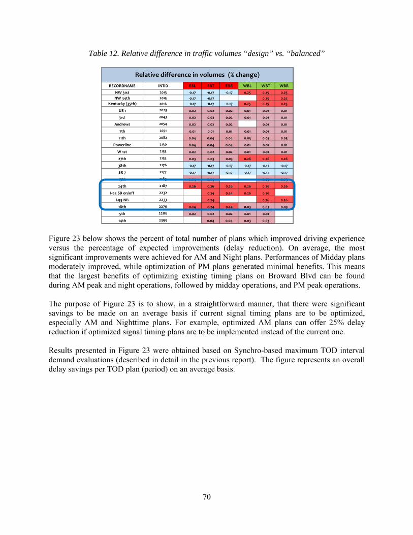
70

Table 12. Relative difference in traffic volumes “design” vs. “balanced”

Figure 23 below shows the percent of total number of plans which improved driving experience versus the percentage of expected improvements (delay reduction). On average, the most significant improvements were achieved for AM and Night plans. Performances of Midday plans moderately improved, while optimization of PM plans generated minimal benefits. This means that the largest benefits of optimizing existing timing plans on Broward Blvd can be found during AM peak and night operations, followed by midday operations, and PM peak operations. The purpose of Figure 23 is to show, in a straightforward manner, that there were significant savings to be made on an average basis if current signal timing plans are to be optimized, especially AM and Nighttime plans. For example, optimized AM plans can offer 25% delay reduction if optimized signal timing plans are to be implemented instead of the current one. Results presented in Figure 23 were obtained based on Synchro-based maximum TOD interval demand evaluations (described in detail in the previous report). The figure represents an overall delay savings per TOD plan (period) on an average basis.

RECORDNAME INTID EBL EBT EBR WBL WBT WBR

NW 31st 2013 ‐0.17 ‐0.17 ‐0.17 0.25 0.25 0.25

NW 34th 2015 ‐0.17 ‐0.17 0.25 0.25

Kentucky (35th) 2016 ‐0.17 ‐0.17 ‐0.17 0.25 0.25 0.25

US 1 2023 0.02 0.02 0.02 0.01 0.01 0.01

3rd  2043 0.02 0.02 0.02 0.01 0.01 0.01

Andrews 2054 0.02 0.02 0.02 0.01 0.01

7th 2071 0.01 0.01 0.01 0.01 0.01 0.01

11th 2082 0.04 0.04 0.04 0.03 0.03 0.03

Powerline 2130 0.04 0.04 0.04 0.01 0.01 0.01

W 1st 2133 0.02 0.02 0.02 0.01 0.01 0.01

27th 2153 0.03 0.03 0.03 0.26 0.26 0.26

38th 2176 ‐0.17 ‐0.17 ‐0.17 ‐0.17 ‐0.17 ‐0.17

SR 7 2177 ‐0.17 ‐0.17 ‐0.17 ‐0.17 ‐0.17 ‐0.17

15th 2185 0.04 0.04 0.03 0.03

24th 2187 0.26 0.26 0.26 0.26 0.26 0.26

I‐95 SB on/off 2232 0.24 0.24 0.26 0.26

I‐95 NB 2233 0.24 0.26 0.26

18th 2270 0.24 0.24 0.24 0.03 0.03 0.03

5th 2288 0.02 0.02 0.02 0.01 0.01

14th 2399 0.04 0.04 0.03 0.03

Relative difference in volumes  (% change)

71

Figure 23. Percent of improvement vs percent of total number of plans improved overall

4.2.6 Application of the method in MS Excel auto-spreadsheet

As an extension of this task, the FAU researchers developed a practical application (MS Excel auto-spreadsheet), in which an operator is able to observe current signal timing plans effectiveness to respond to recent changes in traffic demand. An operator can evaluate the latest changes in daily traffic demand and based on the historical hourly volumes identify the most appropriate signal timing plan for the corresponding demand. In fact, this MS Excel spreadsheet tool can be perceived as some sort of a Traffic Responsive Pattern Selection (TRPS) library of signal timing plans which could help operators identify the most appropriate signal timing plan quickly. Simplified explanation of any TRPS logic is that such systems are based on a “pattern recognition” scheme. This spreadsheet tool uses a similar approach to select the best signal timing plan for a specific traffic demand. It is created as an off-line tool, which uses historical traffic counts (from a group of detectors) to compare them with the most recent traffic volumes and select the best match from the history of available counts. Then, based on this match, the tool proposes a new signal timing plan which was through previous analysis identified as the best signal timing plan for such traffic demand. Once selected, such a plan can be implemented based on the previous days’/weeks’/months’ expected traffic conditions. MVDS traffic counts are retrieved every 15 minutes, 24 hours a day 7 days a week. Figure 24 below shows collected data from each of the observed MVDS detectors (M17, M18, M19, M20, M21).

72

Figure 24. MVDS traffic data for every day and time interval Figure 24 shows traffic flow data in a format where corresponding traffic parameters (speed, volume, occupancy, density) (for EB direction) are reported for every time interval. For the purpose of this activity only traffic volume data are relevant. The user needs to select an appropriate date and time (specific 15-minute interval) which needs to be investigated. This is accomplished by filtering out (Figure 25) particular day and time interval, which results in appropriate MVDS values (shown in Figure 25). At this point, the data is ready to be processed by a macro.

73

Figure 25. MVDS values displayed after filtering MS Excel spreadsheet tool selects specific Signal Timing Plan (STP) to be implemented by finding the best match of the selected volumes with the volumes stored in the database (shown in Figure 25). Concept behind the tool is shown in Figure 26. By clicking on the sheet “calculate” a new sheet window is open showing a reference column (the one which is selected from the field data) in yellow along with all of the other columns (Figure 26).

74

Figure 26. Calculate sheet with reference column In the next step, the values in the reference column are compared with the values in all of the other columns in the worksheet. Each of the columns corresponds to a TOD on a specific day and each consists of exactly 10 MVDS values collected for respective days and TOD periods. Reference column here represents the column which consists of user-selected MVDS values for a specific time period during a specified day. Figure 26 shows that there are 10 MVDS values, representing five detection stations in two directions (Figure 25). Color coded tables in Calculate sheet have been shown only for visualization purposes and each is associated with a specific TOD plan. Root mean square error (RMSE) is calculated for each comparison (between each day and the reference data). In the next step a macro is run to process the comparisons (Figure 27). VBA code for utilizing the STP library is fairly simple - the best match between sets of MVDS data is found (based on the smallest RMSE value) and the most suitable STP is activated. Results of this process are shown in Figure 28. One of the advantages of this method is that it deos not require any microsimulation modeling (VISSIM or similar) but it only requires use of deterministic signal optimization software (Synchro, VISTRO etc.).

75

Figure 27. Macro to identify the best matching volumes

76

Figure 28. Best suitable STP as a result

4.3 Testing of TMC Strategies for Recurring and Nonrecurring Traffic Conditions

4.3.1 Background

The purpose of the task was to qualitatively assess management of available data to improve traffic operations without large investments. This task intended to provide an effective traffic monitoring strategy to the traffic operators in TMC especially in cases where there are not enough ITS infrastructures to identify traffic conditions. For example, Palm Beach County TMC does not possess same level of ITS infrastructure as Broward County TMC does. In Phase 1, the FAU research team developed the demand estimation model using travel time, volume, speed data obtained from the microscopic traffic simulation model (i.e., VISSIM). In phase 2, the team developed the travel time-V/C relationship through existing Volume-Delay Functions (VDFs) based on the field-collected traffic data. The FAU research team identifies the specific signatures of eight traffic scenarios developed in Phase 1. While the simulation output data were used to find the signatures in Phase 1, the field detection data are being used in Phase 2 to fine-tune the signatures identified. The following ATMS data sources were identified as particularly useful along Broward Blvd:

1. Bluetooth BlueTOAD (Traffic Cast): the Bluetooth travel time origin and destination (BlueTOAD) devices detect anonymous Bluetooth signal from mobile devices (cell phones, tablets, laptops, etc.) inside vehicles. The devices can collect travel time, speed, and origin-destination (O-D) data from the field.

2. Microwave Detector Stations (Wavetronix) MVDS: two types of Wavetronix sensors of Smart Sensor V and Smart Sensor HD have been installed in the Broward County. Smart Sensor V can accurately monitor up to eight lanes of traffic and can collect volume, speed, occupancy, and vehicle classification from the field. Smart Sensor HD can monitor up to 22 lanes of traffic. They can record volume, average speed, occupancy, 85th percentile, average headway, average gap, speed bin counts, direction counts, and classification counts.

3. SunGuide (Florida Intelligent Transportation System): an ATMS software that helps FDOT to control and monitor roadside equipment and vehicle resources on the Interstate System. The software facilitates traffic and incident management in the state of Florida. It also disseminates traveler information to the monitoring public. The software communicates with Road Rangers and supports I-95 express lane pricing. Multiple traffic control and management devices are controlled by SunGuide such as dynamic message signs, variable speed limit signs, toll message signs, and ramp signals.

4. ATMS.now (Trafficware): a central management system used by the Broward County TMC to control and manage traffic signals. The system communicates with Naztec traffic controllers remotely and enables traffic operators to change the signal timing in real-time. The systems also enable operators to provide Closed Circuit TV (CCTV) surveillance footage. Also, Changeable Message Signs (CMS) are controlled using the software. Broward County has about 1,300

77

signal controllers, where almost half of them have been transferred to the new ATMS.now system.

FAU research team identified specific signatures of eight traffic scenarios developed in Phase 1. While the simulation output data were used to find the signatures in Phase 1, the field detection data are being used in Phase 2 to fine-tune the signatures identified. To this end, the team is collecting the detectable traffic data from the Broward County TMC. Figure 29 shows the plotting results of travel time and estimated V/C collected on April 30 2015 from SW 22nd Ave to NW 18th Ave on Broward Blvd. This road segment is where traffic congestion frequently occurs due to the traffic from I-95 northbound off-ramp and the school zone. Parts of Figure 29 were created to find the signatures of oversaturation, the red-colored lines are absolute values of traffic parameter and the black-colored lines are relative values that are changes per minute. Note that the data smoothing technique was applied to clearly identify the changes in traffic parameters by a specific time unit. From the figures, two peaks (i.e., morning and evening peaks) are articulately shown in terms of both travel time and V/C ratio. The oversaturation is shown when travel time and V/C ratio are higher than approximately 150 seconds and 1.2, respectively.

(a) Original T.T. data (b) 15-Min. Smoothed T.T. data (c) 30-Min. Smoothed T.T. data

(c) Estimated V/C Ratio (b) 15-Min. Smoothed V/C (c) 30-Min. Smoothed V/C

Figure 29. Data Smoothing Results using Travel Time and Estimated V/C An automated data post-processing program was developed to investigate daily/monthly/seasonal variations in traffic parameters (i.e., volume, occupancy rate, speed,

78

travel time) and the changes in traffic signal timing parameters (i.e., cycle length and phase duration) when a specific traffic event occurred. This program operates with the following steps.

1) Loading the source data retrieved from BlueTOAD, MVDS, and ATMS.now 2) Integrating the data collected from different data sources. 3) Filtering and sorting the particular data collected during the incident 4) Reformatting the captured data into an appropriate data format 5) Plotting the data using Matlab or Excel.

Figure 30 shows the plotted traffic matrices developed by the automated data post-processing program using the field data including the saturated congestion. Figure 30 shows the changes of travel time/volume/speed at every road section on Broward Blvd using the colored-legend. The upper matrix was created under the normal condition, and the lower matrix was created under the saturated condition, for the same weekday during morning peak hour. No unusual traffic activity was detected aside from the increase in traffic demand during rush hour (7:00am to 8:00am). As shown in these two matrices, the difference between the normal and saturated conditions can be clearly identified. Note that the base data for these matrices are also stored as a .txt file format.

Figure 30. Traffic Detection Matrix

In addition, Figure 31 was developed to identify how signal timing plans responded to the saturated condition at the specific signalized intersection. Figure 31 shows changes in cycle

Occupancy rate

Occupancy rate

79

length, the durations of phases 2 (eastbound) and 6 (westbound), and their percentages as parts of the cycle length. Cycle length and phase duration changes occurred as a result of fluctuations in the peak-hour traffic demand.

Figure 31. Changes in ATMS.now Signal Timings due to Increase in Traffic Demand Based on Figures 30 and 31, and their counterparts for other traffic situations, the FAU team has quantified traffic signatures for the eight traffic scenarios, which was documented in the final report for the previous phase of this project. The initial version of an automated data post-processing program was modified over time to better handle detection data outputs. The FAU research team continued to develop the, and it was enhanced to handle the field detection data obtained from a single detection point as well as the

80

data from an entire corridor. Currently, there are 5 mid-block detectors collecting volume, speed, and occupancy rate, and 6 Bluetooth detection points covering 5 travel time measurement sections on Broward Blvd. Based on these field detection data, the program extracts only the data from a specific detection point according to what user specified in the program. Figures 32 and 33 show traffic metrics from a single detector along Broward Blvd. Traffic signatures for a specific type of congestion or incident were identified using similar traffic metrics from various detectors.

a)

b)

Figure 32. Volume and speed from a single detector during an incident

0

50

100

150

200

250

300

34200 34800 35400 36000 36600 37200 37800 38400 39000 39600

Volume (Veh

icles)

Simulation Time (Seconds)

VOLUME

BASE INCIDENT

0

5

10

15

20

25

30

35

40

34200 34800 35400 36000 36600 37200 37800 38400 39000 39600

Speed (MPH)

Simulation Time (Seconds)

SPEED

BASE INCIDENT

81

a)

b)

Figure 33. Travel time and occupancy from a single detector during an incident

0

50

100

150

200

250

300

350

400

450

500

34200 34800 35400 36000 36600 37200 37800 38400 39000 39600

Travel Tim

e (Seconds)

Simulation Time (Seconds)

TRAVEL TIME

BASE INCIDENT

0

10

20

30

40

50

60

70

80

34200 34800 35400 36000 36600 37200 37800 38400 39000 39600

Occupan

cy Rate (%)

Simulation Time (Seconds)

OCCUPANCY RATE

BASE INCIDENT

82

In addition, MATLAB-based visualization module was improved to include the occupancy rate measurements in the plotted graphs, and not to indicate the detection-blind areas as shown in Figure 34.

Figure 34. Traffic detection matrix for event traffic In the next step, the source code of the automated data post-processing program was modified to generate visually-improved traffic performance matrices. This program basically reads the traffic detection data (i.e., volume, occupancy rate, speed, and travel time) obtained from the Broward TMC and generates traffic parameters’ signatures for a pre-determined date and time t. Based on these basic functionalities, the program is capable of generating the data table as well as the graphical plots including the color scheme legend. Also, this program was modified to produce the comparison matrix that shows the changes of traffic parameters compared to normal day traffic. The team is expecting that the traffic signatures of various incident types can readily be identified using these graphical plots and the data tables. Figures 35 and 36 show the example plots including the traffic performance matrices and the comparison matrices produced from the congestion incident occurred on Broward Blvd. It should be noted that the traffic congestion occurred at NW 7th Avenue at 8:43 A.M. on July 9th, 2014, and it continued 82 minutes, according to the event chronology report from the Broward County Traffic Management Center (TMC). The automated data post-processing program was created to generate visually-improved traffic performance matrices, based on traffic detection data (i.e., volume, occupancy rate, speed, and travel time). As explained in earlier reports program creates the traffic parameters for a specific date and pre-defined by the user. The program is able to produce the distribution of traffic parameters for a specific day, thus enabling the conditions to be observed and compared with normal day conditions. Furthermore, the program produces the comparison matrix which displays relative and absolute changes in the parameters for the two selected days. By using these plots the user is able to identify traffic signatures of various incident types or special events.

Occupancy rate 

 

Occupancy rate 

 

83

Figure 35. Example of traffic incident signature plot – July 9th, 2014

Normal Day - Eastbound July 9th - Eastbound

84

Figure 36. Example of traffic incident signature comparison plot – July 9th, 2014

Figures 37 and 38 show example plots including the traffic performance matrices produced for the congestion occurred on Broward Blvd. It should be noted that the traffic congestion occurred on I-95 Avenue at 16:17 P.M. on September 12th, 2014, and it continued for 368 minutes, according to the event chronology report from the Broward County Traffic Management Center (TMC). This is the reason why this particular incident’s traffic parameter were plotted and shown below.

85

Normal Day - Westbound September 12th Westbound

Figure 37. Example of traffic incident signature plot – September 12th, 2014

4.4 Validation of the Simulated Traffic Management Center Strategies

4.4.1 Background

This task stands to provide a comprehensive TMC plan for managing recurring and non-recurring traffic events. Task was initiated by identifying the field-data based traffic signatures that have been conducted in Task 4. The FAU research team needed to provide a valid traffic simulation model for the TMC operators to obtain accurate results from the experiments with traffic alternatives. After the traffic simulation model is validated, the TMC operators will have a valid test-bed to experiment various traffic strategies before the real-world implementation. Accordingly, the Broward Blvd VISSIM simulation model is being enhanced by comparing the simulated traffic detection data with the field detection data obtained from the Broward county TMC.

86

Figure 38. Example of traffic congestion signature comparison plot – September 12th, 2014

4.4.2 VISSIM model validation (new ITS data)

The FAU research team validated the Broward Blvd traffic simulation model developed in Phase I, using a new set of field-detection data. The new set of data included several months of MVDS detector and BlueTOAD travel time data. Ultimate purpose of validation was to equip TMC operators with a reliable simulation test-bed so that they can experiment with various traffic strategies prior to implementing them in the field. Simulation model is validated for a normal traffic condition, and the results are shown in Figure 39.

87

Figure 39. Model Validation Results – August data

88

For a more reliable simulation test-bed, the simulation model needed to be validated for a normal day traffic. July data that the FAU team had collected previously, were not appropriate as the validation data because the traffic demand does not reach as expected due to school summer breaks along Broward Blvd. Therefore, the team decided to use the August data to validate the model, and developed the MS-Excel-based calculation sheet for automating the validation process when the data is ready. Later, the team used September, October and November data to further validate the model, thus making it more reliable. Average travel times during these three months were taken into consideration for validation purposes. These months most accurately represent usual traffic patterns and changes in daily traffic flow. MS-Excel-based calculation sheet for automating the validation process was also implemented and validation progress is shown on the charts below (Figure 40).

Figure 40. Early stage validation progress Also, traffic volume check was performed as part of the model’s validation procedure. Its purpose was to determine how well the simulation outputs match the real-world turning movement counts. Traffic counts for each intersection approach were compared against the field data for each TOD period investigated in 15 minutes increments. Figure 41 shows the scatter plots of the validated turning movement counts for Broward Blvd.

89

Figure 41. Broward Blvd traffic volume check

4.4.3 Traffic event scenarios

The other portion of this task validated the Broward Blvd microsimulation model using the new set of field-collected data for various traffic event scenarios. For several scenarios current field signal timings and traffic volumes have been modified to correspond, as close as possible, to specific event day traffic conditions. The FAU research team evaluated appropriate strategies through software-in-the-loop simulation environment. Software-in-the-loop (SIL) simulation was utilized for the purpose of accomplishing the task of easy implementation and replicate actual TMC operating settings. The FAU research team used 4 months of data to determine adequate demand for specific event scenarios. Average travel times during these three months were taken into consideration for validation purposes. The FAU research team has investigated the relationship between travel times collected in the field and those observed in microsimulation. The field travel times include both: GPS travel time measurements as well as segment travel times collected between pairs of Bluetooth devices. GPS travel times were used, as a more accurate source of data, to calibrate intersection-to-intersection travel times in the simulation model, which are necessary to estimate effectiveness of strategies for recurring and non-recurring traffic conditions. The segment travel times from Bluetooth devices were utilized to validate the travel times from the microsimulation model.

90

Figure 42 represents the comparison between GPS and VISSIM measured travel times between adjacent pairs of intersections. Segment travel times have been also compared to corresponding Bluetooth segment travel times. These are represented in Figure 43.

a)

b)

Figure 42. Travel time validation (GPS vs VISSIM) for EB a) and WB b) directions

91

a)

b)

Figure 43. Travel time validation (Bluetooth vs VISSIM) for EB a) and WB b) direction

4.4.4 Methodology

In this task, recurring and nonrecurring traffic scenarios are identified with the microsimulation model. The scenarios are identified using the literature and BCTED input. Another important factor in determining the location of the scenarios was the proximity of the field detectors to the sensor location because the scenarios need to be monitored closely and appropriate signatures should be captured. Each scenario is modeled in the VISSIM microsimulation model, and respective demand threshold and strategies are identified. The recurring scenarios include base and over-saturated scenarios, and nonrecurring scenarios are arterial incidents, and event traffic congestion scenarios.

92

1. Base scenario: In this scenario, all links in the microsimulation model are operating in the under-saturated condition. All other scenarios are compared to this scenario. Traffic is controlled by software in the loop (SIL) simulation, and management objective is to provide maximum progression in the arterial system.

2. Oversaturated: The volume is considerably higher than the capacity, and queue spills to the upstream intersection in one or two links. Traffic is controlled by an Operator in the Loop (OIL) system. In this condition, queues have already formed, and they would not dissipate unless a certain strategy is implemented. Therefore, the objective is to manage the queue efficiently in the system to avoid gridlock.

3. Arterial incidents: Similar to freeway incidents, arterial incidents can also impose a considerable amount of delay on the transportation network. Since the speed limits on the surface streets are usually lower than on freeways, the severity of such incidents is less than freeway incidents. The FAU research team identified arterial incidents locations based on the historical data acquired from BCTED.

4. Event traffic: Traffic events can also create a severe congestion inside the transportation network. Art performances, festivals, and sport competitions are common examples of special events that happen inside of the transportation network. Traffic in this scenario will be controlled by OIL. The management objective is to manage queues in the transportation system. The location of the event traffic scenario was determined based on the BCTED input.

4.4.5 General approach

General approach in determining adequate congestion alleviation strategies for specific traffic conditions:

1. Insert balanced traffic volumes and current signal timings into VISSIM model 2. Observe network performance outputs (baseline) 3. Recreate most frequently occurring traffic events scenarios (i.e. incident) 4. Observe network performance outputs (incident scenario) 5. Compare simulation results from these two VISSIM files 6. Implement congestion mitigation strategy (TMC operators*) 7. Observe network performance outputs (strategy implemented) 8. Quantify network performance benefits (“no strategy” vs. “strategy”) 9. Implement newly developed strategy 10. Demonstrate that new strategy produces better traffic performance metrics (reduction

in delay, increase in throughput and speed etc.) when compared to currently implemented strategies*

All scenarios are modeled in the Broward Blvd. VISSIM model. For each defined traffic scenario, traffic conditions are captured by monitoring selected MOEs such as speed and volume. The FAU research team has developed a tool to monitor key performance measures in VISSIM. The specific behavior of selected performance measures is recorded and termed as “scenario signature” in this study. Each scenario is expected to have a special signature. Traffic scenarios are described in the following:

93

1. Base: In this scenario, all the links in the simulation model are operating in the undersaturated conditions. The operational objective is to provide maximum progression in the system of arterial streets. All other scenarios are compared to this scenario to determine specific signatures of other scenarios. These signatures are captured by monitoring several performance measures such as: speed, volume, occupancy, and travel time. 2. Oversaturated: In this scenario, the volume is considerably higher than the capacity and queue spills to the upstream intersection in one or two links. Traffic is controlled by an OIL system. Queues have already formed and they are not dissipating unless a certain strategy is implemented. Therefore, an objective is to manage the formed queues efficiently in the system. Effective strategies in this case are retiming signals and utilizing DMS.

1. Increase the input volume near 50% 2. Identify time period when the arterial becomes saturated 3. Capture the oversaturated scenario signature 4. Identify thresholds 5. Evaluate strategies

4.4.5.1 Base Scenario

In this scenario all the links are operating in the undersaturated condition and volume over capacity ratio is less than one in all the links. All other scenarios are compared to this scenario. Three base scenarios are modeled as follow:

1. Broward Blvd. Model in the Morning Peak 2. Broward Blvd. Model in the Evening Peak 3. Network Model in the Evening Peak

4.4.5.2 Oversaturated Scenario

This scenario is similar to the saturated scenarios except that the volume is increased from 20% to 50% of the original value. Queues are being formed, but they do not dissipate unless a certain strategy is implemented. From the traffic management perspective, the objective is to manage the formed queues efficiently in the system. This scenario was run as an extension to the saturated scenario in Broward Blvd. simulation model. Figure 44 shows scope of saturated and oversaturated scenarios inside the simulation model. Field Bluetooth detectors are shown by (B) and the mid-block detectors are represented in (M). Figure 45 shows the location of saturated and oversaturated scenarios. The scenarios are modeled for entire Broward Blvd. corridor.

94

Figure 44. Saturated and oversaturated scenarios scope in the simulation model

Figure 45. Saturated and oversaturated scenario location

95

4.4.5.3 Arterial Incident Scenario

Arterial incidents impose a significant delay to the transportation network. Arterial incidents are usually less severe than freeway incidents. Also, the incident clearance time is usually shorter than the freeway incident. In order to select an appropriate location to simulate the incident in VISSIM, historical data were acquired from FDOT. The FAU research team analyzed incident data from Broward Blvd. Event logs during a four month long period in 2014 in the study area, as well as field data collected in the same period. In this research, the FAU research team was interested in analyzing link data since it is more frequent and incident clearance is more challenging task. To this end, the following intersections in the Broward Blvd. had the highest total number of link incidents:

1. I-95 SB (Broward Blvd. EB) 2. Powerline (Broward Blvd. EB) 3. SW 18th Ave. (Broward Blvd. WB) 4. SW 15th Ave. (Broward Blvd. WB)

All of the intersections presented above were considered as a potential arterial incident location. The Powerline intersection was selected (Figure 46) as an incident location since there was adequate ITS infrastructure to closely monitor the scenario and develop appropriate traffic management strategies.

Figure 46. Arterial incident scenario location Arterial incident scenario was emulated by parking spaces. A single parking space was created to block the leftmost lane. The incident duration was adjusted by modifying dwell time parameter.

96

Also, multiple routing decisions were linked to the parking lot. Figure 47 below shows a screenshot of the arterial incident scenario in the simulation model.

Figure 47. Arterial incident scenario in the simulation model

Arterial incident scenario has two sub-scenarios with different durations of 30 and 60 minutes, which are shown in Table 13.

Table 13. Arterial Incident Sub-Scenarios

Number Duration(minutes) Time Simulation Time

Location Method

1 30 min. 8:00-8:30

8100-9900 Broward Ave & Powerline Rd EB

Blocked single lane using a parking space 2 60 min. 8:00-

9:008100-11700

4.4.6 Scenario-Based Analysis

The results of the scenario analyses are presented in this section. The signature of each scenario is captured by monitoring traffic performance measures such as throughput, occupancy rate, speed, and travel time. Appropriate threshold for each performance measure is identified and documented. For each scenario, certain strategies are identified to alleviate the congestion. The effectiveness of the strategies is evaluated using the simulation models. The performance measures are retrieved from the field and simulation detectors inside simulation model. Table 14 summarizes scenarios considered in this study.

97

Table 14. Summary of considered scenarios

# Congestion

Type Name Description

1

Non

recu

rrin

g

R

ecur

ring

Base This is a normal condition, which all the links are

operating in the undersaturated mode.

2 Saturated Queue forms and dissipates in some of the intersections

sporadically.

3 Oversaturated Queue spillbacks to the upstream intersection in one or

more links.

4 Work Zones Arterial capacity reduced due to lane blockage

5 Arterial

Incidents Incidents, which occur on the arterial corridors.

6 Event Traffic Special events such as art performances, festivals, and

athletic games.

The base scenario represents the normal condition that all the links are operating in the undersaturated condition. This scenario is kept as the base scenario and other scenarios and respective strategies are compared to this scenario. Table 15 presents signal timing pattern in the base scenario. The base scenario signal timing plans are equivalent to existing signal timing plans. The analyses results of other scenarios are presented in this section.

98

Table 15. Signal timing pattern for the Base Scenario

Intersection SC# Ph1 Ph2 Ph3 Ph4 Ph5 Ph6 Ph7 Ph8 C.L.* Offset

SR7 77 26 54 26 48 32 54 26 48 160 88

SW 38th Ave 76 20 79 26 35 20 79 160 84

SW 35th Ave 16 125 35 160 131

SW 34th Ave 15 20 100 120 40 160 151

SW 31st Ave 13 24 70 24 42 24 70 24 42 160 2

Riverland Rd 53 24 77 20 39 24 77 20 39 160 109

SW 24th Ave 87 20 95 45 20 95 45 160 109

I-95 SB/NB 32 20 60 25 55 160 0

SW 18th St 70 15 103 42 15 103 42 160 25

SW 15th Ave 85 25 97 97 38 160 3

SW 14th Ave 99 130 30 130 160 134

NW 11th Ave 82 26 96 38 19 96 38 160 140

Powerline Rd 30 123 37 123 37 160 93

Avenue of the Arts

71 13 71 14 38 21 71 29 38 160 104

NW 5th St 88 106 34 20 106 34 160 78

NW1st Ave 33 84 51 25 84 51 160 51

Andrews Rd 54 23 63 20 43 63 30 43 160 62

NE 3rd Ave 43 20 63 20 47 20 63 30 47 160 129

US1 23 35 47 30 42 25 47 36 42 160 15

* Cycle Length

4.4.6.1 Saturation and Oversaturation Scenarios

The saturation and oversaturation scenarios were modeled inside the Broward Blvd. model from 8:00 to 9:00 AM. The scope of the scenarios was entire Broward Blvd. corridor. The models were created inside the simulation model by increasing the volume by 20%. The control objective for these scenarios is queue management. The queue management strategy applies only for the main road queues. The field sensors used in this analysis were M-20 (mid-block detector) and B-27 to B-29 (Bluetooth device). Error! Reference source not found. shows what field-like simulation measurements were used to develop strategies for scenarios with saturated and oversaturated traffic conditions. In order to collect traffic data for these scenarios, volume, speed, and occupancy were collected from the data collection points that correspond to M-20 field detectors. Similarly, the travel times were collected from travel time sections that emulate section covered by the BlueTOAD devices at SW 14th Ave. and Andrews Blvd.

99

Figure 48. Saturation and oversaturation detection strategy

100

5 METHODS FOR TRAFFIC MANAGEMENT CENTERS WITH LIMITED ITS DATA

5.1 Traffic Congestion Analysis Application

Traffic congestion is an inevitable part of the transportation network. With a constant increase in number of drivers, the roadway infrastructure is not able to keep its pace. Recurring and nonrecurring traffic congestions cause oversaturation in the transportation network. Traffic Congestion Analysis application is developed to enable real time traffic congestion estimation using Google Maps traffic layer. It is primarily intended to assist traffic operators in areas without comprehensive coverage with traffic data, especially areas where the need to monitor traffic congestion levels is evident. This tool implements a method to identify traffic conditions from freely available data sources like Google Maps. It is a web-based application which reports current traffic conditions based on total number of pixels in a given area. It captures traffic conditions on certain predefined network links from Google traffic’s color scheme. The team completed the user manual for traffic congestion analysis application in order to ensure straightforward guidance and effortless comprehensible usage of the program. This user manual provides information how the application works and what it should provide to the TMC operators. The manual includes the general program installation process, and the detailed control features describing generating a new map, creating links/intersections/corridors, observing the congestion, and creating output files follow. It also explains the types and formats of output files produced from this congestion analysis program. In addition, the constraints of this program regarding the running environments and the implementation process were included.

5.1.1 Application development

Few first steps in development of this application were summarized as follows.

Displaying link performance (Figure 49) Traffic congestion levels are shown using appropriate color scheme (according to the

percentage of pixels associated with a specific link performance level).

101

Figure 49. Individual link performance is observable in the display

The color scheme associated with specific link performance levels are indicated in Table 16.

Table 16. Relationship between Traffic Condition and Road Segment Color

Warning message at the top of the window was created to avoid simultaneous use of multiple applications on a single computer. Since the web-interface and the main functionality have been already completed, next project period was focused on developing the output file generation module. Basically, the output files were distinguished into the individual link results and the grouped link results. The output file for the individual link results included date, time, link name, # of total pixels captured, # of pixels for normal operation/moderate congestion/high congestion/severe congestion, and their percentage values. The developed output module in the Traffic Congestion Analysis Application creates a folder named using the current system time and stores the output files in that specific folder as shown in Figure 50-(a). The information stored in the output files were also shown in the program’s user interface with the colorful legend and the percentage of roads captured for each legend as shown in Figure 50-(b).

Road Segment Color Traffic Condition Green Normal Operation Yellow Moderate Congestion Red High Congestion Black Severe Congestion

102

(a) Output Files Generated (b) Program User Interface

Figure 50. Traffic Congestion Analysis Application

A congestion warning module was added to the program. This module’s purpose is to warn the TMC operators when the level of congestion in the network is above a specific threshold. The warning message is shown on the window when the percentage of red-colored pixels meets a certain threshold as shown in Figure 51. A random threshold value was used for testing the application. Also, this threshold value is adjustable so TMC operators can modify this value accordingly.

Figure 51. Congestion warning module

In addition, the link selection module was improved to classify the level of analysis in terms of the spatial scope. By grouping the links selected, the traffic analysis can be conducted at the

103

individual link level, the corridor level, the intersection level, and the network level. Based on how the user subdivides the network, the traffic analysis results can be produced by the aggregated level as well as the individual links. Also, the output file format was changed to include the column that indicates the labels of analysis area (i.e., individual link label, corridor label, intersection label, or network label). At the end of development process, the program was enhanced to check multiple links/corridors/intersections in terms of the percentage of severe congestion and to warn the TMC operators by attaching an asterisk to the red-colored cells (i.e., high level of congestion) instead of popping-up multiple additional windows. The threshold of alarm is adjustable by the user, and the program then notice which links/ intersections/corridors have high congestion level above the certain threshold. Figure 52 shows the improved interface of Traffic Congestion Analysis Application.

Figure 52. Interface of Traffic Congestion Analysis Application

5.1.2 Final application and instructions for users

The following is the summary of the latest version of the application package “Traffic Congestion Analysis Application”. Application was successfully applied and tested by Palm Beach County TMC. The latest version of the application package “trafficProject_jar” comes with the following directories and a jar file (Figure 53). To run the application, simply double click and run the trafficProject.jar (Figure 53).

104

Figure 53. Files in the application package

5.1.2.1 Starting the program

1. Click open “trafficProject.jar” file to run the application to get the main menu. 2. The main menu always opens on the second screen/ monitor. The browser with maps must be opened in the main/first screen or else you will receive a capture error. If second screen does not exist, all the items open in the first screen (Figure 54).

Figure 54. Main menu opens on second screen if exist The main menu interface looks like in Figure 55.

Figure 55. Main Menu Window The user chooses whether to “Create a new Subnetwork”, “Load an existing Subnetwork” or “Run an automated traffic analysis from configuration file”.

105

5.1.2.2 Creating a new Subnetwork

Click “Create New Subnetwork” to open the window in Figure 56. Click button “View Map” and define area to be analyzed by clicking on the map

opened (Figure 57) and retrieve new zoomed map center’s latitude and longitude.

Figure 56. Create new subnetwork *Please note the zoom value has to be more than 15 in order to get the best results.

Figure 57. Link monitoring window after clicking “Create New Subnetwork” on main menu Provide the parameters “Name” (with no spaces/use “_” to concatenate words) and “Coordinates” in the textbox as shown in Figure 58. Click “Save”. When “Save” is clicked, the map is saved and the window redirects to the link monitoring window which is discussed later in following section (Figure 59).

106

Figure 58. Coordinates of the chosen center and zoom are displayed above the map

5.1.2.3 Load Existing Subnetwork

Figure 59. Load existing subnetwork This feature of the application is used for analyzing an existing saved map (Example the map created in Figure 58). Upon clicking the button, choose a map from the “Select Map” window (Figure 60) to open the “Link Monitoring” window for analysis (Figure 61).

107

Figure 60. Select Map window

Figure 61. Link monitoring window for the chosen map from “Select Map” window

5.1.2.4 Top panel menu buttons:

Click on “+ Link” button to create a new link, corridor or intersection, and enter a name for it (Figure 62).

Click “Save” to save the link (Figure 62). Click “Ok” to save or “Cancel” to return to last saved condition.

Click “Undo” to remove the unsaved link (Figure 62). To remove a link, select a link from drop down menu and click “-Link” (Figure 62).

108

Figure 62. Operations with links on Link Monitoring window

5.1.2.5 Bottom panel menu Button:

Use the button “Click here to capture congestion on the links” below the map (Figure 63), in order to analyze the traffic for the selected map and output results to right-side panel (Figure 64).

Figure 63. Clicking on the button to start capturing congestion metrics

109

Figure 64. Congestion metrics on the right side of Link Monitoring window

Select specific link/corridor/intersection from drop-down list and click “Add a link” button to insert selected link/corridor or intersection in the scrollable table on the right (Figure 65).

Insert time interval in seconds in the text box next to T-interval label (# 1 in the figure below) to determine the frequency of automatic map updating. Minimum updating time period is 20 seconds (Figure 65).

Insert threshold for high congested links (warning trigger) in the text box labeled HCt-hold (#2) (Figure 65).

Click on “Click here to start capturing congestion on the links” button to start retrieving traffic layer’s # of pixels and estimating levels of congestion for listed entities (Figure 63).

Figure 65. Warning message when threshold is not set

110

Levels of congestion are displayed in columns designated as %N - for normal traffic conditions (green colored), %M - for moderate congestion (orange colored), %H - for heavy congestion (red colored), and %S - for severe, (dark red colored) for every corresponding link. Indicated level of congestion is expressed in %. This data is updated within the time interval defined/indicated in the text box labeled T-interval (Figure 66).

Click on “Stop capturing” button (Figure 66), to stop analysis.

Figure 66. Capturing congestion levels and displaying results in side panel.

Marked with an asterisk, violet cells indicate severely high level of congestion. I.e. congestion level exceeds the threshold set by the user.

Upon clicking on “Stop capturing” button, three types of output files are generated in subfolder with current date’s name (Figure 67).

Figure 67. Output files generated in folder maps

111

The three types of output files are:

Levels of congestion for the selected group of links, intersections and/or corridors, Individual Links performance and Links where pre-determined thresholds were reached.

5.1.2.6 Run Configuration

When clicked on “Run Configuration”, it automates the entire process of picking up Subnetworks and Links, capturing the traffic congestion and displaying the congestion results in a tabular format (Figures 68 & 69). *Please make sure the browser is in maximized mode and opens on main screen.

Figure 68. Functionality of “Run Configuration” button

112

Figure 69. Tabular output by the process to show the results

After every iteration, the browser with title “Traffic” closes and reopens for the next cycle of results of updated Google maps.

All the results are also output to the log files in directory “maps” with a subdirectory named as current date (Figure 70).

Figure 70. Screenshot of log files

113

The automated process basically reads the information provided in a Configuration file.

A new folder named “Config Files” is added to project with “Config_file.txt” (Figure 71) which contains the Subnetwork names and links.

5.1.2.7 Format of Config file:

First Line has to always mention the “Threshold”. Second Line gives the “Time Interval”. The following lines have “Subnetwork” names with .xml as extension and the “Link”

names separated by a delimiter “;”. The maps run in an indefinite loop until the user shuts down the table to stop the

process.

Figure 71. Configuration file example

5.2 Visualization of Traffic Incidents based on SunGuide-like Incident Database

5.2.1 Background and task description

There were two major parts of this task. One was the incident record management system for filtering the incident records, locate in the map, and identify ‘hot-spots’ (i.e., dangerous area). The other was to review existing incident management strategies and investigate the effectiveness of these strategies. Regarding the incident record management system, the web-based user interface was developed to enable the TMC operators to filter/sort the incident data. Incident analysis web application was originally developed using West Palm Beach incident database, but considering SunGuide’s database compatibility, the application is proven to be beneficial to Broward County’s traffic operations staff as well. Web application, in the first place, is intended to enable necessary crash analysis with stored geo-coded historical incident information and hot-spot area identification. The program enables the user to investigate incidents’ location and filter the data by type, date, time and location. The data sorted can be shown in Google map so that the TMC operators can easily determine where the ‘hot-spots’ are during a specific season. The existing incident management system stores not only the incident location, time, and details of the incident but also the traffic strategies implemented against the incident happened. The traffic strategies include increasing cycle length or a specific phase duration for a better progression and mitigating the impact of incident.

114

5.2.2 Development and characteristics of the application

Considering current TMC, FAU team find out that current incident data archiving system does not store the geo-coded information (i.e., X & Y coordinates) for the incident records, and it lacks the data handling functionalities such as filtering and sorting. These data handling functionalities are important to identify ‘hot-spots’ where the probability of crashes is relatively higher than other areas. Therefore, the FAU research team started working on development of the incident data management program to enhance the existing incident data archiving system by adding the following functionalities.

Filtering and sorting the incident data by incident spots, date & time, types, severity (referring by lane blockage)

Visualizing incidents with a graphical legend on Google map using the geo-coded information

Identifying and indicating ‘hot-spots’ on Google map by considering the number of incidents and severity

Figure 72 below shows the initial design of Incident Record Management System

Figure 72. Initial Design of Incident Record Management System

In the next step in application design, the team enhanced the program to display all incident locations that the user selected (Figure 73). By indicating all incidents occurred during a specific time period, it is expected for the TMC operator to readily identify ‘hot-spot’ which has a high probability of incidents.

115

Figure 73. Initial Design of Incident Record Management System After described enhancements, the following two functionalities were developed: data filtering functionality and data locating functionality. Through these functionalities, the user can filter the incident data by the attributes including the incident types, date, and time, and indicate the selected incident data on the Google map. Incidents at this stage were only indicated with the place mark (Figure 74).

Figure 74. Interface of the Incident Record Management System

116

Aside from the filtering by ID of the incident, time, date and type of the incident, additional filter was developed - the location of the incident was on (Figure 74). Also, the color of the place mark differs depending on the type of the incident. These place marks are supplemented with info boxes encompassing all relevant information for the incident being clicked on the map. The visual appearance of the new info boxes is displayed on Figure 75.

Figure 75. Graphical User Interface for the Incidents Management System

5.2.3 User guide for the Incident Management System

Recommendations provided by PBC and BC TMCs were taken into consideration and appropriate changes have been made. The latest version of the tool was delivered to corresponding TMCs along with supplemental documentation such as instructions and implementation manual as well as technical requirements. This tool has been made available for testing and pending future suggestions and/or advisement will undergo further adjustments in the next period. Incident analysis web application was originally developed using West Palm Beach incident database, but considering SunGuide’s database compatibility, the application is proven beneficial to Broward County’s traffic operations staff as well. Web application is intended to enable necessary crash analysis with stored geo-coded historical incident information and hot-spot area identification. The program enables the user to investigate incidents’ location and filter the data by type, date, time and location. The following is the procedure for using the application:

1. Copy application folder on hard disk. 2. Run application in Visual Studio.

117

3. In SQL server create database labeled Incidents with one table labeled TrafInc1. The table TrafInc1 can be created using the appropriate SQL procedure.

Required data format is shown in Table 17, below.

Table 17. Data format requirements Field name Format ID integer ordering number (ex. 1, 2, 3,…) Date short date format mm/dd/yyyy Time-from short time format hh:mm (24 hour clock format) Time-to short time format hh:mm (24 hour clock format) Location string with maximum length of 60 characters IncidentType string with maximum length of 50 characters Direction string with maximum length of 60 characters LaneBlockage string with maximum length of 60 characters CCTV string with maximum length of 60 characters SignalTimingChanges string with maximum length of 100 characters Benefits string with maximum length of 100 characters Latitude a decimal number with a precision of 8 and scale of

6 (8,6) Longitude a decimal number with a precision of 8 and scale of

6 (8,6) SQL procedure for creating this table will be delivered to the users along with database, as well as the rest of the SQL procedures, which are indispensable and used by the program.

4. When application is run for the first time, table containing incident data in user’s

interface is empty. In order to populate the table, press the “Choose file” button and select the file containing incidents data in .csv format.

5. Import the data from the file selected by clicking the “Import” button. 6. If the .csv file does not contain incident’s location latitude and longitude information as is

the case in the figure below, these data should be entered by choosing an incident from the dropdown list “Select an incident by ID” (Figure 76) and dragging the incident icon on the map, in order to obtain the geo-coded location in the corresponding text boxes for latitude and longitude.

118

Figure 76. Selecting an incident by ID

7. Press “Update” button to save these values in the database. 8. Corresponding options i.e. dropdown lists, enable the data to be filtered by date, type,

time interval or incidents’ location, and displayed respectively on the map. *Every incident is represented by a different marker according to its type. Otherwise, if the type is not defined in the table, incident is represented with standard red colored Google Maps icon. 9. By clicking on incident icon, an Info window is opened (Figure 77), listing all

available information regarding the specified incident.

119

Figure 77. Info box contents for the selected traffic event

5.2.4 Technical requirements

Browser requirements (any of the following):

Google Chrome

Internet Explorer

Firefox

Operating system

Windows operating system

Server requirements

Web application should be hosted on server/cloud

Database requirements

SQL server database

Input files requirements

Text files in .csv or .txt format

Filtering option was later enhanced to offer simultaneous filtering by date and time (Figure 78), although the possibility for filtering only by date or time still persists (Figure 79 and 80). Simultaneous filtering by date and type is also allowed.

120

Figure 78. Filtering by date and time simultaneously

Figure 79. Filtering by time frame when the incident happened and ended

Figure 80. The text file in .csv format representing the filtering for the chosen time frame Also, the application reads the existing ID of the incident from Metrics/SunGuide table instead of creating the ID automatically (Figure 80).

121

Figure 81. The ID of the incident is the same as in the text file in .csv format The tabular visualization of the incidents’ data has also been improved; the name of the intersection where the incident occurred was included in the table (Figure 82).

Figure 82. The intersection name is added in the tabular visualization of the incidents Source file in .csv format, as well as the SQL table which contains incidents’ data is also supplemented with the name of the intersection. Aside from this, the manual and prerequisites for using this application have been improved as well.

5.3 Triggering Mechanisms to Assist Traffic Management Center Operators

The triggering strategies are based upon travel time data which can readily be collected in the field by utilizing either the BlueTOAD database or the Traffic Congestion Analysis Application. For capturing the travel time data from Google Map, the team developed the Traffic Congestion Analysis Application in the task 9. The collected travel time data are used to estimate V/C, an indicator of traffic condition, using the relationship between travel time and V/C which were developed in the task 4. Therefore, when the estimated V/C ratio reaches certain threshold, the traffic operator in TMC needs to take certain actions. Figure 83 shows the conceptual diagram about how the traffic strategies are triggered using V/C levels. V/C estimation methodology using the relationship between travel time and V/C was developed to effectively operate the signalized intersection at the microscopic level while the Traffic Congestion Analysis Application was developed to monitor the network-wide traffic conditions at the macroscopic

122

level by taking advantage of the Google traffic’s color scheme. Therefore, the triggering mechanism is initiated from the traffic analysis results of these two programs.

Figure 83. Traffic Strategies Triggering Procedure The basic triggering mechanism consists of four procedures: 1) Monitoring traffic conditions through the V/C estimation and Traffic Congestion Analysis Application, 2) Checking threshold to determine triggering timing, 3) Investigation and confirmation of the traffic situations if alarms are issued through the threshold check process, and 4) Taking actions (i.e., traffic strategies) according to the traffic operational manual. This task was conducted by connecting with Tasks 2, 3 and 9. This was because the triggering mechanism is initiated by the estimated V/C and the network performance level. For example,

123

both the V/C estimation program and the Traffic Congestion Analysis Application warn the TMC operators based on the pre-defined threshold values of V/C ratio and the percentage of congestion in the particular network. To this end, the ‘warning’ functionality was developed and added into both programs. Note that the default threshold values are pre-determined, but these threshold values are adjustable in the program. In addition, the triggering mechanism essentially includes two aspects: Operator-in-the-Loop (OILS) and the System-in-the-Loop (SILS). For example, there are some traffic events for which traffic parameters pattern recognition is relatively straightforward since traffic parameters’ signatures before and after the event are clearly distinct and, on the other hand some traffic events are even scheduled (i.e. transit priority). However, there are various traffic conditions that do not have clear traffic signatures and OILS must be considered in these cases. Triggering mechanism is initiated through traffic monitoring. Thus, the traffic situation identification process, which is the beginning point of the triggering mechanism, was designed within three-level monitoring process as follows. 1. Network-wide monitoring 2. VDF-based intersection performance evaluation 3. Identification of traffic scenarios using field traffic signatures First, to automate the process between the network-wide monitoring and the signal performance evaluation, the interface between the traffic congestion analysis applications and the VDF-based signal performance monitoring program was developed. Therefore, if a specific corridor or area has been detected as a severely congested area, then the automated interface guides the user into the signal performance monitoring program for examining V/C ratio, Level of Service (LOS), and the number of cycles of the subject intersection. Through this process, the TMC operators can notice which intersection is the most problematic and needs to be treated by traffic strategies. Under this task to date, two warning functionalities were developed. One was developed as part of traffic congestion analysis web application which triggers operator’s attention when certain user-defined congestion-level threshold has been reached. The application allows for user-defined thresholds to be established on every link/segment/corridor individually. Each time the application is running these can be altered as needed. For example, a “30% threshold” (meaning that more than 30% of a link is color coded in red) can mean adverse traffic operations on that link while the same threshold may not mean any significant degradation on the other link(s). The other warning functionality was defined as part of the travel time-based signal performance measures tool and it was intended to warn operators whenever intersection approach V/C levels reached pre-defined values. Specifically, threshold levels were commonly defined to be over 1 (V/C>1). There were no other warning functionalities identified. Also, due to idiosyncratic nature of these tools and dynamic mechanisms that they support, FAU researchers were not able to recommend specific values for the thresholds mentioned above. Such threshold values should be either based on engineering judgment of the operators (after a longer use of these tools), or based on some sort of future sensitivity analysis.

124

6 CONCLUSIONS

Considering width and variety of topics covered in this research, a conclusion section could be very long and could address the details of various methods and strategies. However, such long conclusions are beyond the scope of this report. The authors constrain conclusions presented below only to major methods/applications developed during the research. For each method and application we provide conclusions about success of the experiments and achieved results and their major limitations. Also, each of the methods and applications is accompanied with some ideas for future improvement and implementation.

6.1 Estimating Signal Performance based on Link Travel Times

Purpose of this method was to enable use of commonly available point-to-point travel times to estimate performance of traffic signals. The method was proven to be very successful. The FAU researchers were able to estimate signal’s through movement V/C ratio, Level of Service, and number of cycles necessary to pass through the signal; all based on link travel times. In addition, as a secondary achievement, the FAU researchers came up with a revised Volume-Delay function that was shown to perform better than the traditional BPR function. However, the major problem with this approach is availability of data. The method works well only after significant calibration and validation that includes long data collection and reduction processes. Also, the system is supposed to have point-to-point travel time measuring devices at each intersection and signal timing data available on a cyclical basis from the central traffic signal platform. Although this tool shows a lot of promises for future use, very few agencies have right now corridors which are so heavily equipped with ITS technologies to enable successful implementation of this method. Future reduction in the costs of travel time measurement devices, as much as wider availability of high-precision travel time data from web applications (e.g. Google and similar) may yield this method to be more implementable. The FAU research team recommends that future deployments of ITS/ATMS equipment are executed in such a way to comprehensively cover smaller spatial areas instead of stretching the ITS infrastructure over larger areas. This particular method requires travel time measuring devices at each signalized intersection and video detection that can recognize length of the queues and can be used to measure stop-line saturation flow rates.

6.2 Refinement of Signal Timing Plans based on Available ITS Data

This method was developed to assist operators in evaluation of the current signal timing plans based on the traffic flows which are observed from MVDS detectors. A library of plans was developed (each of which reflects the best theoretical solution e.g. Synchro or Vistro) and integrated in the spreadsheet that is able to recognize which signal timing plan is the best for the set of traffic volumes which are the closest to the MVDS volumes retrieved from the field. Theoretical practicality of this method is great because it can show the operators whether the current signal timing plan is good or not so good, as well as how much savings (% of the difference in Performance Indices can be achieved if a different plan is selected. Frequency of

125

reported savings can show whether a certain signal timing plan needs to be closely reviewed and potentially replaced. Applicability of this method/tool again depends on availability of ITS data, which in this case represent multiple MVDS system detectors on a corridor. More detectors are present, more accurately and uniquely are traffic conditions represented and a better match is achieved between traffic conditions and proposed signal timing plan. Another issue is applicability of signal timing plans developed by deterministic tools such as Synchro and Vistro. These tools often cannot reflect idiosyncrasies and details of the real-world traffic conditions and can, sometimes, propose signal timing plans that do not work in reality. Future of this concept needs to be determined after its practical implementation and use by traffic signal operators at Southeast Florida TMCs. The operators may find this tool very practical and a good indicator of the quality of signal timing plans. Thus, it is recommended that this tool is installed and tested in TMC environment. Once the operators provide enough feedback about functionalities and reasonableness of this tool it can be improved to help operators identify quality of signal timings which are run in the field conditions.

6.3 Testing of TMC Strategies for Recurring and Nonrecurring Traffic Conditions

In this task our team worked on testing some of the signal timing and other strategies in simulation environment. The results have shown significant improvement over running existing signal timing plans when working under a variety of nonrecurring and recurring traffic event scenarios. The biggest issue that we encountered in this task is that exercises that we performed in the lab cannot easily reflect field conditions. In spite of the fact that we were able to change in real-time signal timing parameters to reflect traffic during events, which itself is a major achievement as not many research groups can perform this type of control, we were not able to use the exact platform that is available in Southeast Florida traffic signal jurisdictions – ATMS.now. The problem is simply that ATMS.now is not available for use in the Software-in-the-Loop simulation. Another issue was ability to replicate the exact same traffic events that have been occurring in the field. Although our simulation experiments were quite successful in a couple of cases, there are many traffic events (especially nonrecurring) which are very difficult to model with the use of base traffic model case developed for normal conditions. Simply said, once the model is calibrated for normal conditions it can be used (reliably) only for small deviations from such conditions and the large shifts (either temporal or spatial) in traffic demands are difficult to be predicted. This method still holds a lot of promises but its full implementation would require availability of ATMS.now as a SIL platform and potentially development of a connection between microsimulation system and a real-time feed from field data (MVDSs and travel time readers). FAU research team recommends that FDOT TMC operator review the way they report incidents and other events in the SunGuide system. It seems that information about length and extent of the incidents would be helpful to completely understand impact of such traffic events.

126

6.4 Validation of the Simulated Traffic Management Center Strategies

As mentioned in the previous paragraphs, validation of the simulated traffic management strategies was constrained by FAU team’s ability to replicate field conditions both on traffic side (making sure that simulation replicates field measurements) and traffic control side (use the same platform for ad-hoc changes in signal timings to respond to the traffic events). Our ability to replicate the field conditions was documented with relatively high statistical precision in a couple of scenarios where overall traffic demand did not deviate too much from the base conditions. For the other cases, it seemed that traffic conditions were so different that our base model did not make a lot of sense. However, we faced a bigger challenge on traffic control side where we could not exactly replicate dynamics of ATMS.now signal timing plans in the field because of unavailability of ATMS.now for use in simulation software. Thus, FAU team was constrained to use Virtual next Phase software from Siemens to resemble signal timing plans from ATMS.now. Although the overall engine (based on NEMA operations) should be similar we cannot say with confidence that we were able to achieve what operators can do with ATMS.now in the field. This particularly refers to setting alarms and triggers which would enable operators to automatically execute certain control commands (e.g. increase split or reduce cycle length) when a relevant traffic event occurs. This method still holds a lot of promises but for its full success it is necessary to have a higher level of cooperation with third-party vendors which was not possible in this project (it was beyond its scope). The main recommendation for this activity is that FDOT invest in research to find out which of the existing signal-simulation interfaces would be the best to use to investigate impact of operators’ (signal timing) strategies on traffic conditions. This can be achieved through a highly-calibrated simulation study where operator’s signal actions can be performed as the simulation runs. Current ATMS.now setup limits options to model exact field signal timings in simulation environment.

6.5 Traffic Congestion Analysis Application

Purpose of this application is to provide some means, to traffic operators of the agencies which do not have a comprehensive (or any) ITS data coverage, to assess level of congestion on the networks under their jurisdiction. The application captures color of color-coded links on Google maps to estimate percentage of congestion on the network of user’s choice. The network can be as small as single link or as large as the entire jurisdiction. When a larger network is analyzed the application considers several smaller networks separately and cycles through them to provide an overall network congestion assessment. The program, well described in the report, provides several configuration features to address users’ needs. Although this program makes a revolution in how the available data can be used to assess no congestion with a very small investment it does relay on traffic data streams hosted by third parties. Also, the method of retrieving congestion information is not exact and prone to errors and changes in the third-party business applications and decisions (e.g. if Google changes their congestion color just slightly the program would need to be modified).

127

This tool still represent one of the key outputs of this research and creates a promise for many agencies with little or no ITS data. Currently, the FAU team has deployed this tool at the Palm Beach County TMC and we expect to get feedback how to improve/modify this tool to meet expectations and needs of TMC operators. It is recommended that this method is further investigated and applied in field-like environment on continual basis to gather feedback from the operators and improve this tool. The tool should be redesigned to be compatible with FDOT database platforms to enable creation of various queries and customized reports and trend analysis of the performance metrics. Also, there is need to investigate potential of this tool for estimation of the impact of traffic signal strategies in a manner of before/after studies and its interfaces with other traffic data platforms, such as SunGuide/ATMS data, WAZE, etc.

6.6 Visualization of Traffic Incidents based on SunGuide-like Incident Database

Purpose of this activity was to use visualization of the incident records, stored in SunGuide-like database developed for Palm Beach County, to identify ‘hot-spots’ in traffic operations (i.e., places where many incidents occur) and apply some strategies accordingly. Development of the tool was a success and the tool exhibited all of the intended features. Although there is a potential for future improvement it is not clear whether PBC and other agencies in vicinity, will be fully migrating their operations to SunGuide, in which case this tool may become unnecessary. FAU expects to get feedback about this tool and its potential improvement sometimes soon after which it will be possible to assess tool’s future and further intended activities. The FAU research team recommends that this SunGuide-like incident database is further improved and provided to agencies around Florida, which do not have access to SunGuide but have a need for similar tool to visualize traffic and incident data. Further markers and legends can be added to make further cross-references between incident spots and locations of other traffic-related features. In overall, it can be concluded that this research project went more into width (than depth) of the objective to propose, develop, and test various methods and applications to assist traffic operators of various agencies in Southeast Florida to monitor and manage arterial operations. Variety and the quality of the tools developed, for a number of idiosyncratic requests and positions, document the seriousness of the faced problems and the needs for continuous work on improvement of the existing tools and development of the new ones. In order to find more about these methods and tools, and to make a request to download applicable tools, files and user manuals please contact Dr. Aleksandar Stevanovic at astevano@fau.edu or on the phone (561) 297-3743.

128

7 REFERENCES

3M. 2014. (a web page) http://www.3m.com/3M/en_US/company-us/, St. Paul, MN, 3M Co

(accessed September 10th, 2014). Acyclica Analyzer. 2014. (a web page) https://www.acyclica.com/products/acyclica-analyzer,

Frisco, CO, Acyclica Inc. (accessed September 16th, 2015). Acyclica. Acyclica Analyzer User Guide. Frisco, CO, Acyclica Inc.2014.

http://www.acyclica.com/?page_id=617 (accessed February 20th, 2014). Akcelik, Rahmi. "Travel time functions for transport planning purposes: Davidson's function, its

time dependent form and alternative travel time function." Australian Road Research 21, no. 3 (1991).

ARH Inc.2014. (a web page) http://www.arh.hu/, Budapest, Hungary, ARH Inc. (accessed

September 26th, 2014). Bosch. Bosch Video Client - Bosch Security Systems. Stuttgart, Germany, Robert Bosch

GmbH.2014. www.resource.boschsecurity.com. (accessed February 18th , 2014). Cetin, Mecit, Peter Foytik, Sanghoon Son, Asad J. Khattak, Robert Michael Robinson, and

Jaesup Lee. "Calibration of Volume-Delay Functions for Traffic Assignment in Travel Demand Models." In Transportation Research Board 91st Annual Meeting, no. 12-0132. 2012.

Cetin, Mecit. “Optimization of Volume-Delay Functions and Their Implementations in VDOT

Travel Demand Models.” Paper presented at Symposium on Transportation Issues and Problems Hampton Roads, October 1st, 2010.

Connected Signals. 2015. ( a web page) https://connectedsignals.com/enlighten.php, Eugene,

OR, Connected Signals (accessed February 5th, 2015). Dowling, Richard, and Alexander Skabardonis. "Urban arterial speed-flow equations for travel

demand models." Innovations in Travel Demand Modeling(2008): 109-113. Dowling, Richard, Rupinder Singh, and Willis Cheng. "Accuracy and performance of improved

speed-flow curves." Transportation Research Record: Journal of the Transportation Research Board 1646 (1998): 9-17.

Fambro, Daniel, and Nagui Rouphail. "Generalized delay model for signalized intersections and

arterial streets." Transportation Research Record: Journal of the Transportation Research Board 1572 (1997): 112-121.

129

Foytik, Peter, Mecit Cetin, and Robert Michael Robinson. "Calibration of BPR Function Based on Link Counts and Its Sensitivity to Varying Demand." InTransportation Research Board 92nd Annual Meeting, no. 13-4019. 2013.

He, Nan, and Shengchuan Zhao. "Discussion on Influencing Factors of Free-flow Travel Time in

Road Traffic Impedance Function." Procedia-Social and Behavioral Sciences 96 (2013): 90-97.

Horowitz, Alan J. "Delay/volume relations for travel forecasting based upon the 1985 Highway

Capacity Manual." FHWA Report (1991). Huntsinger, Leta, and Nagui Rouphail. "Bottleneck and Queuing Analysis: Calibrating Volume-

Delay Functions of Travel Demand Models." Transportation Research Record: Journal of the Transportation Research Board 2255 (2011): 117-124.

Klieman, Lee, Wang Zhang, Vincent L. Bernardin Jr, and Vladimir Livshits. "Estimation and

comparison of volume delay functions for arterials and freeway HOV and general purpose lanes." In Transportation Research Board 90th Annual Meeting, no. 11-0242. 2011.

Kurth, David, At Van den Hout, and Berry Ives. "Implementation of Highway Capacity Manual-

based volume-delay functions in regional traffic assignment process." Transportation Research Record: Journal of the Transportation Research Board 1556 (1996): 27-37.

Li, Jing, Nagui Rouphail, Andrzej Tarko, and Leonid Velichansky. "Overflow delay model for

signalized arterials." Transportation Research Record: Journal of the Transportation Research Board 1555 (1996): 1-8.

Manual, Highway Capacity. "Highway Research Board." Special Report 87 (1965): 1965. Manual, Traffic Assignment. "Bureau of Public Roads." US Department of Commerce (1964). MathWorks. Curve Fitting Toolbox User Manual. Natick, MA, The MathWorks Inc, 2014. http://www.mathworks.com/products/curvefitting/. (accessed on March 5th ,2014). MetroTech Net. 2014. (a web page) http://metrotech-net.com/, Alpharetta, GA, MetroTech Net.

(accessed September 25th, 2014). Park, Byungkyu Brian, and Yin Chen. Quantifying the benefits of coordinated actuated traffic

signal systems: A case study. No. VTRC 11-CR2. 2010. Park, Byungkyu, and J. D. Schneeberger. Evaluation of traffic signal timing optimization

methods using a stochastic and microscopic simulation program. Virginia Transportation Research Council, 2003.

130

PTV. VISUM User Manual Version 7.50. Karlsruhe, Germany, PTV AG, 2001. http://visiontraffic.ptvgroup.com/en-us/training-support/support/ptv-visum/(accessed on

February 3th, 2014). QvisionTechnology. Examination of the methods and costs of providing traveler information.

Chula Vista, CA, Qvision Technology, 2014. http://www.qvisiontechnology.com/Documents/QVISION_TRAVELER_INFO_SURVEY_JULY2014a.pdf (accessed September 13th, 2014).

Sensys Networks. Sensys Networks VDS240 Wireless Vehicle Detection System Traffic - DOT

2 Set Up and Operating Guide. Berkeley, CA, Sensys Networks Inc. 2011. http://www.precisiontrafficsafety.com/wp-content/themes/theme-precisiontraffic-3.6/downloads/Sensys_TrafficDOT_2.0_UserGuide.pdf (accessed September 15th, 2014).

Sensys_Networks. Sensys Whitepapers. Berkeley, CA, Sensys Networks Inc. 2014.

http://www.sensysnetworks.com/services_support/ (accessed Februaary 21st , 2014). Singh, Rupinder, and R. Dowling. "Improved speed-flow relationships: application to

transportation planning models." In Seventh TRB Conference on the Application of Transportation Planning Methods. 2002.

Skabardonis, Alexander, and Richard Dowling. "Improved speed-flow relationships for planning

applications." Transportation Research Record: Journal of the Transportation Research Board 1572 (1997): 18-23.

Spiess, Heinz. "Technical note—Conical volume-delay functions."Transportation Science 24,

no. 2 (1990): 153-158. Stevanovic, Aleksandar. "Assessing Deterioration of Pretimed, Actuated-Coordinated, and

SCOOT Control Regimes in Simulation Environment." PhD diss., The University of Utah, 2006.

TrafficCast. (2012a). BlueTOAD Cut Sheet. Madison, WI, TrafficCast, 2012.

http://trafficcast.com/products/view/blue-toad/ (accessed December 15th, 2012). TrafficCast. Bluetooth Travel-time Origin And Destination. Madison, WI, TrafficCast, 2012.

http://trafficcast.com/products/view/blue-toad/ (accessed December 14th, 2012). Trafficware. ATMS.now brochure. Sugar Land, TX, Trafficware, 2013.

www.trafficware.com/documents/ (accessed December 20th, 2013). TRB. Highway Capacity Manual 2010. Washington, DC, TRB.org, 2014.

http://www.trb.org/Main/Blurbs/164718.aspx (accessed March 1st, 2014). Willmott, Cort J. "On the validation of models." Physical geography 2, no. 2 (1981): 184-194.

131

Xiong, Hui, and Gary Davis. "Field evaluation of model-based estimation of arterial link travel times." Transportation Research Record: Journal of the Transportation Research Board 2130 (2009): 149-157.

Yun, Seongsoon, Wade White, Daniel Lamb, and Yongqiang Wu. "Accounting for the impact of

heavy truck traffic in volume-delay functions in transportation planning models." Transportation Research Record: Journal of the Transportation Research Board 1931 (2005): 8-17.