matrix functions in lingo · matrix functions in lingo starting with lingo 16, a variety of matrix...
TRANSCRIPT

Matrix Functions in LINGO
Starting with LINGO 16, a variety of matrix functions are
available, including:
Matrix multiply, @MTXMUL
Inverse, @INVERSE
Transpose, @TRANSPOSE
Determinant, @DETERMINANT
Eigenvalue/Vector, @EIGEN
Cholesky Factorization, @CHOLESKY
Regression, @REGRESS
Positive Definiteness constraint, @POSD.
Keywords: Matrix multiply, Inverse, Transpose, Determinant, Eigenvalue, Cholesky Factorization, Regression, Positive Definite’

How Do I Find the Available Functions in LINGO?
Where Do I Find Complete Examples of Usage?
Two Places:
1) www.lindo.com click on:
MODELS Keywords index topic
2) Samples subdirectory if you have already installed LINGO.
Names of relevant models are listed in the examples that follow.
Usage:
The matrix functions can be used only in CALC sections, with
one exception. @POSD can be used only in a MODEL section.

Transpose of a Matrix
! Illustrate Transpose of a matrix.(TransposeOfMatrix.lng)
Example: We wrote our model assuming
distance matrix is in From->To form,
but now we have a user who has his
matrix in To->From form;
SETS:
PROD; ! List of products;
PXP( PROD, PROD): DIST, TOFDIST;
ENDSETS
DATA:
PROD =
VANILLA BUTTERP, STRAWB, CHOCO;
! A changeover time matrix. Notice,
changing from Choco to anything else
takes a lot of cleaning.
‘From’ runs vertically, ‘To’ runs horizontally;
DIST=
0 1 1 1 ! Vanilla;
2 0 1 1 ! ButterP;
3 2 0 1 ! StrawB;
5 4 2 0; ! Choco;
ENDDATA
CALC:
@SET( 'TERSEO',2); !Output level (0:verb, 1:terse, 2:only errors, 3:none);
@WRITE( 'Changing from a row to a column', @NEWLINE(1));
@TABLE( DIST);
@WRITE( @NEWLINE(1),' The transpose( To->From form)',@NEWLINE(1));
TOFDIST = @TRANSPOSE( DIST); !Take the transpose of DIST; @TABLE( TOFDIST);
ENDCALC

Changing from a row to a column
VANILLA BUTTERP STRAWB CHOCO
VANILLA 0.000000 1.000000 1.000000 1.000000
BUTTERP 2.000000 0.000000 1.000000 1.000000
STRAWB 3.000000 2.000000 0.000000 1.000000
CHOCO 5.000000 4.000000 2.000000 0.000000
The transpose( To->From form)
VANILLA BUTTERP STRAWB CHOCO
VANILLA 0.000000 2.000000 3.000000 5.000000
BUTTERP 1.000000 0.000000 2.000000 4.000000
STRAWB 1.000000 1.000000 0.000000 2.000000
CHOCO 1.000000 1.000000 1.000000 0.000000
Transpose of a Matrix
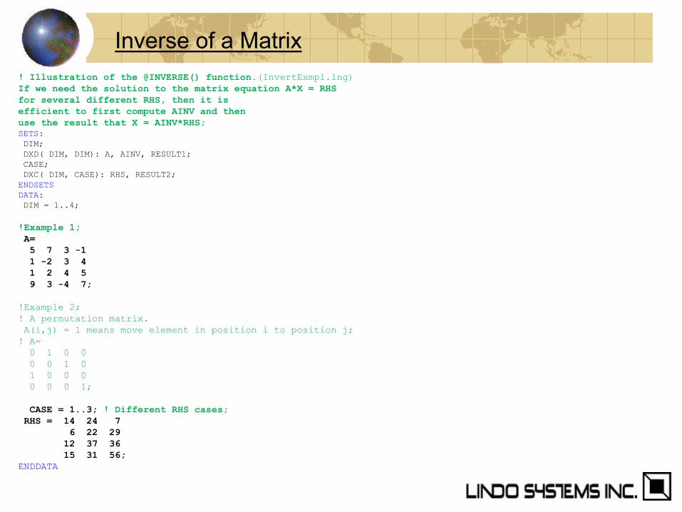
! Illustration of the @INVERSE() function.(InvertExmpl.lng)
If we need the solution to the matrix equation A*X = RHS
for several different RHS, then it is
efficient to first compute AINV and then
use the result that X = AINV*RHS;
SETS:
DIM;
DXD( DIM, DIM): A, AINV, RESULT1;
CASE;
DXC( DIM, CASE): RHS, RESULT2;
ENDSETS
DATA:
DIM = 1..4;
!Example 1;
A=
5 7 3 -1
1 -2 3 4
1 2 4 5
9 3 -4 7;
!Example 2;
! A permutation matrix.
A(i,j) = 1 means move element in position i to position j;
! A=
0 1 0 0
0 0 1 0
1 0 0 0
0 0 0 1;
CASE = 1..3; ! Different RHS cases;
RHS = 14 24 7
6 22 29
12 37 36
15 31 56;
ENDDATA
Inverse of a Matrix
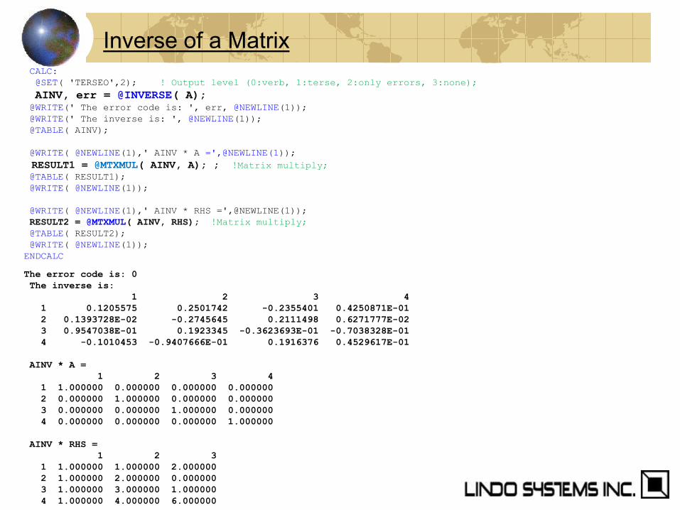
CALC:
@SET( 'TERSEO',2); ! Output level (0:verb, 1:terse, 2:only errors, 3:none);
AINV, err = @INVERSE( A); @WRITE(' The error code is: ', err, @NEWLINE(1));
@WRITE(' The inverse is: ', @NEWLINE(1));
@TABLE( AINV);
@WRITE( @NEWLINE(1),' AINV * A =',@NEWLINE(1));
RESULT1 = @MTXMUL( AINV, A); ; !Matrix multiply; @TABLE( RESULT1);
@WRITE( @NEWLINE(1));
@WRITE( @NEWLINE(1),' AINV * RHS =',@NEWLINE(1));
RESULT2 = @MTXMUL( AINV, RHS); !Matrix multiply;
@TABLE( RESULT2);
@WRITE( @NEWLINE(1));
ENDCALC
The error code is: 0
The inverse is:
1 2 3 4
1 0.1205575 0.2501742 -0.2355401 0.4250871E-01
2 0.1393728E-02 -0.2745645 0.2111498 0.6271777E-02
3 0.9547038E-01 0.1923345 -0.3623693E-01 -0.7038328E-01
4 -0.1010453 -0.9407666E-01 0.1916376 0.4529617E-01
AINV * A =
1 2 3 4
1 1.000000 0.000000 0.000000 0.000000
2 0.000000 1.000000 0.000000 0.000000
3 0.000000 0.000000 1.000000 0.000000
4 0.000000 0.000000 0.000000 1.000000
AINV * RHS =
1 2 3
1 1.000000 1.000000 2.000000
2 1.000000 2.000000 0.000000
3 1.000000 3.000000 1.000000
4 1.000000 4.000000 6.000000
Inverse of a Matrix

! Using Cholesky Factorization to Generate (CholeskyNormal.lng)
Multi-variate Normal Random Variables with a
specified covariance matrix.
Using matrix notation, if
XSN = a row vector of independent random variables
with mean 0 and variance 1,
and E[ ] is the expectation operator, and
XSN' is the transpose of XSN, then its covariance matrix,
E[ XSN'*XSN] = I, i.e., the identity matrix with
1's on the diagonal and 0's everywhere else.
Further, if we apply a linear transformation L,
E[(L*XSN)'*(L*XSN)]
= L'*L*E[XSN'*XSN] = L'*L.
Thus, if L'*L = Q, then the
L*XSN will have covariance matrix Q.
Cholesky factorization is a way of finding
a matrix L, so that L'*L = Q. So we can think of L as
the matrix square root of Q.
If XSN is a vector of standard Normal random variables
with mean 0 and variance 1, then L*XSN has a
multivariate Normal distribution with covariance matrix L'*L;
Cholesky Factorization: Generate Correlated R.V.s

DATA:
! Number of scenarios or observations to generate;
SCENE = 1..8000;
MU = 50 60 80; ! The means;
! The covariance matrix;
Q = 16 4 -1
4 15 3
-1 3 17; SEED = 26185; ! A random number seed;
! Generate some quasi-random uniform variables in interval (0, 1);
XU = @QRAND( SEED);
ENDDATA
CALC:
! Compute the "square root" of the covariance matrix;
L, err = @CHOLESKY( Q);
@SET( 'TERSEO',3); ! Output level (0:verb,1:terse,2: only errors,3:none);
@WRITE(' Error=', err,' (0 means valid matrix.', @NEWLINE(1));
@WRITE(' The L matrix is:', @NEWLINE(1));
@TABLE( L); ! Display it;
! Generate the Normal random variables;
@FOR( SCENE( s):
! Generate a set of independent Standard ( mean= 0, SD= 1)
Normal random variables;
@FOR( DIM( j):
XSN(j) = @PNORMINV( 0, 1, XU(s,j));
);
! Now give them the appropriate means and covariances.
The matrix equivalent of XN = MU + L*XSN;
@FOR( DIM( j):
XN(s,j) = MU(j) + @SUM( DIM(k): L(j,k)*XSN(k));
);
);
Cholesky Factorization: Generate Correlated R.V.s

The Q matrix is:
1 2 3
1 16.00000 4.000000 -1.000000
2 4.000000 15.00000 3.000000
3 -1.000000 3.000000 17.00000
Error=0 (0 means valid matrix found).
The L matrix is:
1 2 3
1 4.000000 0.000000 0.000000
2 1.000000 3.741657 0.000000
3 -0.2500000 0.8685990 4.022814
The empirical means:
50.00002 59.99982 79.99992
Empirical covariance matrix:
1 2 3
1 15.99428 4.006238 -0.9971722
2 4.006238 15.00404 2.972699
3 -0.9971722 2.972699 16.98160
Cholesky Factorization: Generate Correlated R.V.s

! Compute the eigenvalues/vectors of a covariance matrix.
(EigenCovarMat3.lng).
Alternatively, do Principal Components Analysis.
If there is a single large eigenvalue for the covariance
matrix, then this suggests that there is a single factor,
e.g., "the market" that explains all the variability;
! Some things to note,
1)In general, given a square matrix A, then we try to find
an eigenvalue, lambda, and its associated eigenvector X,
to satisfy the matrix equation:
A*X = lambda*X.
2) the sum of the eigenvalues = sum of the terms on the diagonal
of the original matrix, the variances if it is a covariance
matrix.
3) the product of the eigenvalues = determinant of the original matrix.
4) A positive definite matrix has all positive eigenvalues;
! Keywords: Eigenvalue, PCA, Principal Component Analysis,
Singular value decomposition, Covariance; SETS:
ASSET: lambda;
CMAT( ASSET, ASSET) : X, COVAR;
ENDSETS
Eigenvalues in LINGO

DATA:
! The investments available(Vanguard funds);
ASSET = VG040 VG102 VG058 VG079 VG072 VG533;
! Covariance matrix, based on June 2004 to Dec 2005;
COVAR=
! VG040 VG102 VG058 VG079 VG072 VG533;
!VG040; 0.6576337E-02 0.7255873E-02 -0.7277427E-03 0.6160186E-02 0.5015276E-02 0.1082129E-01
!VG102; 0.7255873E-02 0.8300280E-02 -0.1067516E-02 0.7007361E-02 0.5651304E-02 0.1208505E-01
!VG058; -0.7277427E-03 -0.1067516E-02 0.1366187E-02 -0.1281051E-02 -0.1113421E-02 -0.1179400E-02
!VG079; 0.6160186E-02 0.7007361E-02 -0.1281051E-02 0.1020367E-01 0.8663464E-02 0.1477201E-01
!VG072; 0.5015276E-02 0.5651304E-02 -0.1113421E-02 0.8663464E-02 0.1568187E-01 0.1510857E-01
!VG533; 0.1082129E-01 0.1208505E-01 -0.1179400E-02 0.1477201E-01 0.1510857E-01 0.3002400E-01;
ENDDATA
CALC:
@SET( 'TERSEO', 2); ! Turn off default output;
@SET( 'LINLEN', 100); ! Terminal page width (0:none);
! Compute the eigenvalues and eigenvectors;
LAMBDA, X = @EIGEN( COVAR); ! Get the sum of the variances;
TOTVAR = @SUM( ASSET(j): COVAR(j,j));
CUMEVAL= 0;
@WRITE(' Eigen- Frac- Associated Eigenvector', @NEWLINE(1),
' value tion ');
@FOR( ASSET(j):
@WRITE( @FORMAT( ASSET(j), '%7s'));
);
@WRITE( @NEWLINE(1));
@FOR( ASSET(j):
CUMEVAL = CUMEVAL + LAMBDA(j);
@WRITE( @FORMAT(lambda(j),'6.3f'), @FORMAT( CUMEVAL/TOTVAR,'7.3f'),': ');
@FOR( ASSET(i):
@WRITE(' ',@FORMAT(X(i,j),'6.3f')); );
@WRITE( @NEWLINE(1));
);
@WRITE(' Sum of variances = ', @SUM(ASSET(j): COVAR(j,j)), @NEWLINE(1));
@WRITE(' Sum of eigenvalues= ', @SUM(ASSET(j): LAMBDA(j)), @NEWLINE(1));
ENDCALC
Eigenvalues in LINGO, II
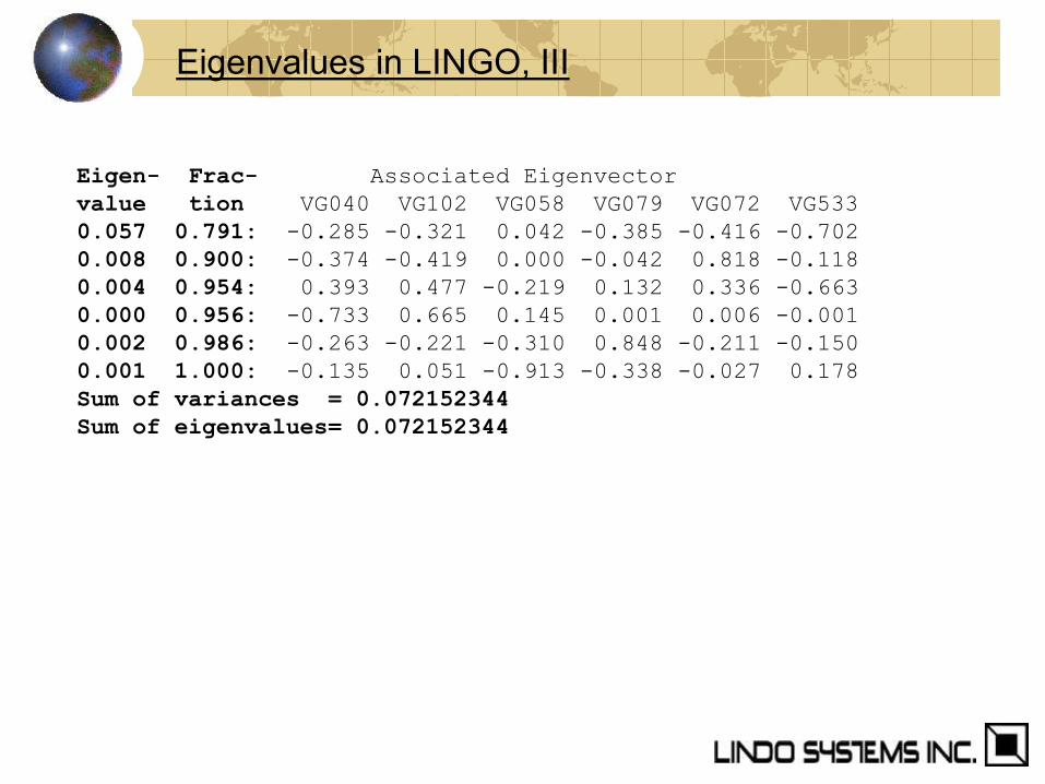
Eigen- Frac- Associated Eigenvector
value tion VG040 VG102 VG058 VG079 VG072 VG533
0.057 0.791: -0.285 -0.321 0.042 -0.385 -0.416 -0.702
0.008 0.900: -0.374 -0.419 0.000 -0.042 0.818 -0.118
0.004 0.954: 0.393 0.477 -0.219 0.132 0.336 -0.663
0.000 0.956: -0.733 0.665 0.145 0.001 0.006 -0.001
0.002 0.986: -0.263 -0.221 -0.310 0.848 -0.211 -0.150
0.001 1.000: -0.135 0.051 -0.913 -0.338 -0.027 0.178
Sum of variances = 0.072152344
Sum of eigenvalues= 0.072152344
Eigenvalues in LINGO, III

Eigenvalues and Dynamic Systems
An important application of eigenvalues is for the modeling of dynamic
systems, - systems that change over time. Suppose we want to model how
populations change over time. E.g., we want to model how the number of
B(t) = bunnies, C(t) = hectares of clover, and F(t) = foxes changes with time
t. We have data that suggest:
B(t+1) = 0.612*B(t) + 2.291*C(t) - 1.200*F(t);
C(t+1) = -0.295 *B(t) + 2.321*C(t) - 0.560*F(t);
F(t+1) = 0.500 *B(t) - 0.050*C(t) + 0.110*F(t)
Thus, if there were only Bunnies and Clover, and no Foxes, Bunnies would do
quite well. Foxes on the other hand depend a lot on Bunnies.
Eigenvalue analysis determines if there is a λ such that B(t+1) = λ*B(t),
C(t+1) = λ*C(t), and F(t+1) = λ*F(t) .
We shall see that whether the population grows with t, (λ > 1), or declines
(λ < 1) depends upon the initial configuration of B(t), C(t), F(t);
.

! Compute eigenvalues and eigenvectors; !(EigenExample.lng);
! Keywords: Eigenvalues, PCA, Population growth;
sets:
item: evalr, evali;
ixi( item, item): a, evecr, eveci;
endsets
data:
item = 1..3; ! The number of items;
! The matrix of interest;
a =
! A population change matrix, P(t+1) = A*P(t);
! Bunnies Clover Foxes;
0.612 2.291 -1.200
-0.295 2.321 -0.560
0.500 -0.050 0.110 ;
enddata
calc:
! Get the
eigenvalues(real part), eigenvectors(real part),
eigenvalues(imaginary part),and eigenvectors(imaginary part);
evalr, evecr, evali, eveci = @eigen(a);
! A scalar Lambda is an eigenvalue, with associated eigenvector P,
if A*P = Lambda*P,
i.e., the proportions of P are unchanged.
They are simply scaled up by Lambda; endcalc
Eigenvalues in LINGO
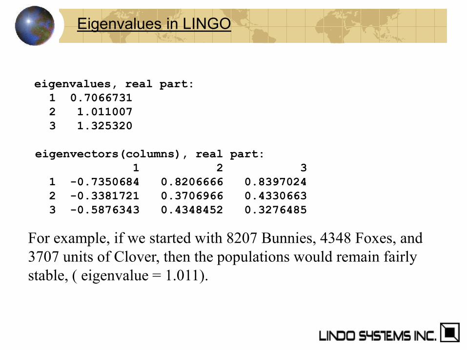
eigenvalues, real part:
1 0.7066731
2 1.011007
3 1.325320
eigenvectors(columns), real part:
1 2 3
1 -0.7350684 0.8206666 0.8397024
2 -0.3381721 0.3706966 0.4330663
3 -0.5876343 0.4348452 0.3276485
Eigenvalues in LINGO
For example, if we started with 8207 Bunnies, 4348 Foxes, and
3707 units of Clover, then the populations would remain fairly
stable, ( eigenvalue = 1.011).

Enforcing Convexity–Positive Definiteness
When discussing positive definiteness of a square matrix, we are
usually concerned with correlation, or more generally, covariance
matrices.
A covariance matrix computed accurately from real data is
automatically positive(semi) definite. Very loosely speaking, the off-
diagonal terms are small in absolute value relative to the diagonal terms.
Example 1: The 2 by 2 matrix
1 x is positive definite if -1 < x < 1.
x 1
Example 2: The 3 by 3 matrix
1 0.9 x is positive definite if 0.62 < x I 1.
0.9 1 0.9
x 0.9 1
I.e., if item 1 has 0.9 correlation with item 2 and item 2 has 0.9
correlation with 3, then 1 and 3 must also be fairly highly correlated.

Enforcing Convexity–Positive Definiteness
Planning under Uncertainty Using Covariance Matrices.
! Make minimal adjustments to an (POSDadjOffDiag.lng)
initial guessed correlation matrix to make it a valid,
Positive Semi-Definite matrix. A non-positive-definite matrix
allows for a (nonsensical) portfolio variance < 0.
Application: If we have an incomplete data set,
e.g., not every variable appears in every observation,
we may be able to get
estimates of every correlation term individually,
however, taken together,
the initial matrix may not be Positive Definite, a feature that
should be true for any correlation or covariance matrix.
So for a correlation matrix, we would like to make minimal
adjustments (move towards 0) of the off-diagonal terms to make
the matrix POSD;
You need POSD for a Local Optimum to be a Global Optimum.
Most Quadratic Programming Solvers require that the
Q matrix be POSD.

SETS:
VEC;
MAT( VEC,VEC) | &1 #GE# &2: QINI, QADJ, QFIT;
ENDSETS
DATA:
VEC = 1..3;
! Our initial estimate of the correlation matrix,
( May not be positive semi-definite);
QINI =
1.000000
0.6938961 1.000000
-0.1097276 0.7972293 1.000000 ;
ENDDATA
! Minimize the amount of adjustments we have
to make to the off-diagonal terms of
our initial estimated matrix...;
MIN = @SUM( MAT(i,j) | i #GT# j: QADJ(i,j)^2);
! Fitted matrix = initial + adjustment;
@FOR( MAT(i,j) | i #GT# j:
QFIT(i,j) = QINI(i,j) + QADJ(i,j);
! Off diagonal adjustments or fitted
might be < 0;
@FREE( QADJ(i,j));
@FREE( QFIT(i,j));
);
! Diagonal terms stay at 1;
@FOR( VEC(i):
QFIT(i,i) = QINI(i,i);
QADJ(i,i) = 0;
);
! The adusted/fitted matrix must be
Positive semi-definite;
@POSD( QFIT);
Enforcing Convexity–Positive Definiteness -II

DATA:
@TEXT() = 'Initial guess at correlation matrix:';
@TEXT() = @TABLE( QINI);
@TEXT() = '';
@TEXT() = 'Adjustment matrix:';
@TEXT() = @TABLE( QADJ);
@TEXT() = '';
@TEXT() = 'Fitted matrix that is POSD:';
@TEXT() = @TABLE( QFIT);
ENDDATA
Global optimal solution found.
Objective value: 0.10040801E-01
Model is a second-order cone
Initial guess at correlation matrix:
1 2 3
1 1.0000000
2 0.69389610 1.0000000
3 -0.10972760 0.79722930 1.0000000
Adjustment matrix:
1 2 3
1 0.0000000
2 -0.59054698E-01 0.0000000
3 0.45718541E-01 -0.66806876E-01 0.0000000
Fitted matrix that is POSD:
1 2 3
1 1.0000000
2 0.63484140 1.0000000
3 -0.64009058E-01 0.73042242 1.0000000
Enforcing Convexity–Positive Definiteness -III
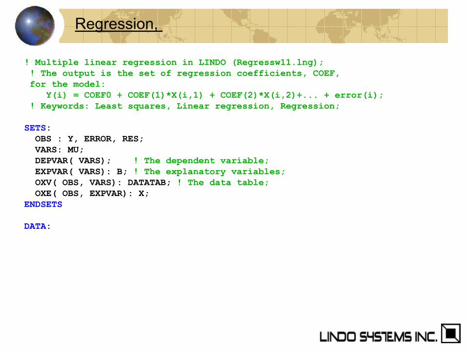
! Multiple linear regression in LINDO (Regressw11.lng);
! The output is the set of regression coefficients, COEF,
for the model:
Y(i) = COEF0 + COEF(1)*X(i,1) + COEF(2)*X(i,2)+... + error(i);
! Keywords: Least squares, Linear regression, Regression;
SETS:
OBS : Y, ERROR, RES;
VARS: MU;
DEPVAR( VARS); ! The dependent variable;
EXPVAR( VARS): B; ! The explanatory variables;
OXV( OBS, VARS): DATATAB; ! The data table;
OXE( OBS, EXPVAR): X;
ENDSETS
DATA:
Regression,

! Names of the variables;
VARS =
EMPLD PRICE GNP__ JOBLS MILIT POPLN YEAR_;
! The (Longley) dataset;
DATATAB =
60323 83 234289 2356 1590 107608 1947
61122 88.5 259426 2325 1456 108632 1948
60171 88.2 258054 3682 1616 109773 1949
61187 89.5 284599 3351 1650 110929 1950
63221 96.2 328975 2099 3099 112075 1951
63639 98.1 346999 1932 3594 113270 1952
64989 99 365385 1870 3547 115094 1953
63761 100 363112 3578 3350 116219 1954
66019 101.2 397469 2904 3048 117388 1955
67857 104.6 419180 2822 2857 118734 1956
68169 108.4 442769 2936 2798 120445 1957
66513 110.8 444546 4681 2637 121950 1958
68655 112.6 482704 3813 2552 123366 1959
69564 114.2 502601 3931 2514 125368 1960
69331 115.7 518173 4806 2572 127852 1961
70551 116.9 554894 4007 2827 130081 1962;
! Dependent variable. Must be exactly 1;
DEPVAR = EMPLD;
! Explanatory variables. Should not include DEPVAR;
EXPVAR = PRICE GNP__ JOBLS MILIT POPLN YEAR_;
ENDDATA
Regression, e.g., Forecasts for Production Planning

CALC:
@SET( 'TERSEO',2); ! Output level (0:verb, 1:terse, 2:only errors, 3:none);
!Set up data for the @REGRESS function;
@FOR( OBS( I):
Y( I) = DATATAB( I, @INDEX( EMPLD));
@FOR( OXE( I, J): X( I, J) = DATATAB( I, J))
);
! Do the regression;
B, B0, RES, rsq, f, p, var = @REGRESS( Y, X);
NOBS = @SIZE( OBS);
NEXP = @SIZE( EXPVAR);
@WRITE( ' Explained error/R-Square: ', @FORMAT( RSQ, '16.8g'), @NEWLINE(1));
@WRITE( ' Adjusted R-Square: ',
@FORMAT( 1 - ( 1 - RSQ) * ( NOBS - 1)/( NOBS - NEXP - 1), '18.8g'),@NEWLINE( 1));
@WRITE( ' Mean square residual: ', @FORMAT(var,'16.8g'), @NEWLINE(1));
@WRITE( ' F statistic: ', @FORMAT( F,'18.12f'), @NEWLINE(1));
@WRITE( ' p statistic: ', @FORMAT( p,'18.12f'), @NEWLINE(2));
@WRITE( ' B( 0): ', @FORMAT( B0, '16.8g'), @NEWLINE( 1));
@FOR( EXPVAR( I):
@WRITE( ' B( ', EXPVAR( I), '): ', @FORMAT( B( I), '16.8g'), @NEWLINE( 1));
);
ENDCALC
Explained error/R-Square: 0.995479
Adjusted R-Square: 0.99246501
Mean square residual: 92936.006
F statistic: 330.285339234521
p statistic: 0.000000000498
B( 0): -3482258.6
B( PRICE): 15.061872
B( GNP__): -0.035819179
B( JOBLS): -2.0202298
B( MILIT): -1.0332269
B( POPLN): -0.051104106
B( YEAR_): 1829.1515
Regression, e.g., Forecasts for Production Planning