lecture i: review of matrix theory and matrix functionsbenzi/web_papers/dob1.pdf · 2014-09-11 ·...
TRANSCRIPT

Lecture I: Review of Matrix Theory and Matrix Functions
Michele Benzi
Department of Mathematics and Computer ScienceEmory University
Atlanta, Georgia, USA
Summer School on Theory and Computation of Matrix Functions
Dobbiaco, 15-20 June, 2014
1

Outline
1 Plan of these lectures
2 Review of matrix theory
3 Functions of matrices
4 Bibliography
2

Outline
1 Plan of these lectures
2 Review of matrix theory
3 Functions of matrices
4 Bibliography
3

Plan and acknowledgements
Lecture I: Review of Matrix Theory and Matrix Functions
Lecture II: Matrix Functions in Network Science, Part 1
Lecture III: Matrix Functions in Network Science, Part 2
Lecture IV: Decay in Functions of Sparse Matrices
Lecture V: Matrix Functions in Quantum Chemistry
Lecture VI: Numerical Analysis of Quantum Graphs
Many thanks to the Organizers of the School and to my collaborators PaolaBoito, Ernesto Estrada, Christine Klymko, Nader Razouk and Mario Arioli. Iwould also like to gratefully acknowledge the early influence of Gene Golub.
4

Gene Howard Golub (1932–2007)
Ghent, Belgium, September 2006 (courtesy of Gérard Meurant)
5

Outline
1 Plan of these lectures
2 Review of matrix theory
3 Functions of matrices
4 Bibliography
6

Matrix classes
Unless otherwise specified, only matrices with entries in R or C will beconsidered.
A matrix A ∈ Cn×n is
Hermitian if A∗ = A
skew-Hermitian if A∗ = −Aunitary if A∗ = A−1
symmetric if AT = A
skew-symmetric if AT = −Aorthogonal if AT = A−1
normal if AA∗ = A∗A
Theorem: A ∈ Cn×n is normal if and only if there exist U ∈ Cn×n unitaryand D ∈ Cn×n diagonal such that U∗AU = D.
7

Jordan Normal Form
Any matrix A ∈ Cn×n can be reduced to the form
Z−1AZ = J = diag (J1, J2, . . . , Jp),
Jk = Jk(λk) =
λk 1
λk. . .. . . 1
λk
∈ Cnk×nk ,
where Z ∈ Cn×n is nonsingular and n1 + n2 + . . .+ np = n. The Jordanmatrix J is unique up to the ordering of the blocks, but Z is not. The λk’sare the eigenvalues of A. These constitute the spectrum of A, denoted byσ(A).
Definition: The order ni of the largest Jordan block in which theeigenvalue λi appears is called the index of λi.
8

Diagonalizable matrices
A matrix A ∈ Cn×n is diagonalizable if there exists an invertible matrixX ∈ Cn×n such that X−1AX = D is diagonal. In this case all the Jordanblocks are 1× 1.
From AX = XD it follows that the columns of X are correspondingeigenvectors of A, which form a basis for Cn.
Normal matrices are precisely those matrices that can be diagonalized byunitary transformations. Thus: a matrix A is normal if and only if thereexists an orthonormal basis for Cn consisting of eigenvectors of A.
The eigenvalues of a normal matrix can lie anywhere in C. Hermitianmatrices have real eigenvalues; skew-Hermitian matrices have purelyimaginary eigenvalues; and unitary matrices have eigenvalues of unitmodulus, i.e., if λ ∈ σ(U) with U unitary then |λ| = 1.
9

Some useful expressions
From the Jordan decomposition of a matrix A ∈ Cn×n we obtain thefollowing “coordinate-free” decomposition of A:
A =s∑
i=1
[λiGi +Ni]
where λ1, . . . , λs are the distinct eigenvalues of A, Gi is the projector ontothe generalized eigenspace Ker((A− λiI)
ni) along Ran((A− λiI)ni) with
ni = index(λi), and Ni = (A− λiI)Gi = Gi(A− λiI) is nilpotent of indexni. The Gi’s are the Frobenius covariants of A.
If A is diagonalizable (A = XDX−1) then Ni = 0 and the expressionabove can be written
A =n∑
i=1
λixiy∗i
where λ1, . . . , λn are not necessarily distinct eigenvalues, and xi, yi areright and left eigenvectors of A corresponding to λi. Hence, A is aweighted sum of at most n rank-one matrices (oblique projectors).
10

Some useful expressions (cont.)
If A is normal then the spectral theorem yields
A =n∑
i=1
λiuiu∗i
where ui is eigenvector corresponding to λi. Hence, A is a weighted sumof at most n rank-one orthogonal projectors.
From these expressions one readily obtains for any matrix A ∈ Cn×n that
Tr(A) :=n∑
i=1
aii =n∑
i=1
λi
and, more generally,
Tr(Ak) =n∑
i=1
λki , ∀k = 1, 2, . . .
11

Singular Value Decomposition (SVD)
For any matrix A ∈ Cm×n there exist unitary matrices U ∈ Cm×m andV ∈ Cn×n and a “diagonal” matrix Σ ∈ Rm×n such that
U∗AV = Σ = diag (σ1, . . . , σp)
where p = minm,n.
The σi are the singular values of A and satisfy
σ1 ≥ σ2 ≥ . . . ≥ σr > σr+1 = . . . = σp = 0 ,
where r = rank(A). The matrix Σ is uniquely determined by A, but U andV are not.
The columns ui and vi of U and V are left and right singular vectors of Acorresponding to the singular value σi.
12

Singular Value Decomposition (cont.)
Note that
Avi = σiui and A∗ui = σivi, 1 ≤ i ≤ p.
From AA∗ = UΣΣTU∗ and A∗A = V ΣT ΣV ∗ we deduce that the singularvalues of A are the (positive) square roots of the eigenvalues of thematrices AA∗ and A∗A; the left singular vectors of A are eigenvectors ofAA∗, and the right ones are eigenvectors of A∗A.
Moreover,
A =r∑
i=1
σiuiv∗i ,
showing that any matrix A of rank r is the sum of exactly r rank-onematrices.
13
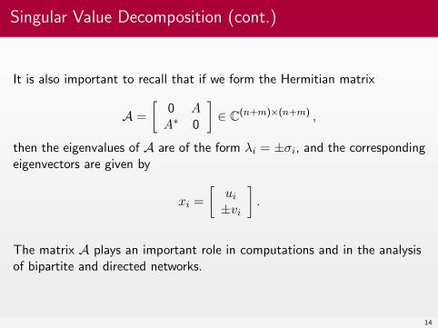
Singular Value Decomposition (cont.)
It is also important to recall that if we form the Hermitian matrix
A =
[0 AA∗ 0
]∈ C(n+m)×(n+m) ,
then the eigenvalues of A are of the form λi = ±σi, and the correspondingeigenvectors are given by
xi =
[ui
±vi
].
The matrix A plays an important role in computations and in the analysisof bipartite and directed networks.
14

Singular Value Decomposition (cont.)
For any matrix A = UΣV ∗ ∈ Cm×n, the Moore–Penrose generalizedinverse (or pseudo-inverse) of A is defined as
A† := V Σ†U∗ ∈ Cn×m ,
where
Σ† := diag (σ−11 , . . . , σ−1
r , 0, . . . , 0) ∈ Rn×m .
The pseudo-inverse is the unique matrix satisfying the following fourconditions:
AA†A = A, A†AA† = A†, (AA†)∗ = AA†, (A†A)∗ = A†A .
When m = n and A is nonsingular, A† = A−1.
15

Schur Normal Form
Any matrix A ∈ Cn×n is unitarily similar to an upper triangular matrix.That is, there exist U ∈ Cn×n unitary and T ∈ Cn×n upper triangularsuch that
U∗AU = T .
Neither U nor T are unique: only the diagonal elements of T are, and theyare the eigenvalues of A.
The matrix A is normal if, and only if, T is diagonal.
If T is split asT = D +N
with D diagonal and N strictly upper triangular (nilpotent), then the“size” of N is a measure of how far A is from normal.
16

Matrix norms
The notion of a norm on a vector space (over R or C) is well-known. Amatrix norm on the matrix spaces Rn×n or Cn×n is just a vector norm ‖ · ‖which satisfies the additional requirement of being submultiplicative:
‖AB‖ ≤ ‖A‖‖B‖, ∀A,B .
Important examples of matrix norms include the induced norms (especiallyfor p = 1, 2,∞) and the Frobenius norm
‖A‖F :=
√√√√ n∑i=1
n∑j=1
|aij |2 .
It is easy to show that
‖A‖1 = max1≤j≤n
n∑i=1
|aij |, ‖A‖∞ = ‖A∗‖1 = max1≤i≤n
n∑j=1
|aij | .
17

Matrix norms (cont.)
Furthermore, denoting by σ1 ≥ σ2 ≥ · · · ≥ σn ≥ 0 the singular values of A, itholds
‖A‖2 = σ1 , ‖A‖F =
√√√√ n∑i=1
σ2i
and therefore ‖A‖2 ≤ ‖A‖F for all A. These facts hold for rectangular matricesas well.
Also, the spectral radius ρ(A) := max|λ| : λ ∈ σ(A) satisfies ρ(A) ≤ ‖A‖ forall A and all matrix norms.
For a normal matrix, ρ(A) = ‖A‖2. But if A is nonnormal, ‖A‖2 − ρ(A) can bearbitrarily large.
Also note that if A is diagonalizable with A = XDX−1, then
‖A‖2 = ‖XDX−1‖2 ≤ ‖X‖2‖X−1‖2‖D‖2 = κ2(X)ρ(A) ,
where κ2(X) = ‖X‖2‖X−1‖2 is the spectral condition number of X.
18

Matrix powers and matrix polynomials
For a matrix A ∈ Cn×n, the (asymptotic) behavior of the powers Ak fork →∞ is of fundamental importance.
More generally, we will be interested in studying matrix polynomials
p(A) = c0I + c1A+ c2A2 + · · ·+ ckA
k .
Let σ(A) = λ1, λ2, . . . , λn, and let A = ZJZ−1 where J is the Jordanform of A. Then p(A) = Zp(J)Z−1. Hence, the eigenvalues of p(A) aregiven by p(λi), for i = 1, . . . , n. Moreover, A and p(A) have the sameeigenvectors. This applies, in particular, to p(A) = Ak.
Thus, if A is diagonalizable with A = XDX−1 then p(A) = Xp(D)X−1.
19

Matrix powers and matrix polynomials (cont.)
We recall the following basic result concerning matrix powers:
Theorem: Let A ∈ Cn×n, then
limk→∞
Ak = 0 ⇔ ρ(A) < 1.
Important: It is sometimes stated that if ρ(A) 1, then the convergenceof Ak to 0 will be very fast. While this is true if A is normal, or “close” tonormal, it is not true in general. For highly nonnormal matrices, theconvergence of Ak to 0 can be extremely slow, even for ρ(A) ≈ 0 (and infact, even for ρ(A) = 0!).
The point is that ρ(A) only governs the asymptotic convergence behaviorof the powers of A, not the transient behavior; in the short term, Ak canhave arbitrarily large entries even if ρ(A) ≈ 0. Moreover, the transientphase can last a long time—i.e., it may take a huge value of k before theasymptotic regime kicks in.
20
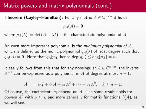
Matrix powers and matrix polynomials (cont.)
Theorem (Cayley–Hamilton): For any matrix A ∈ Cn×n it holds
pA(A) = 0
where pA(λ) := det (A− λI) is the characteristic polynomial of A.
An even more important polynomial is the minimum polynomial of A,which is defined as the monic polynomial qA(λ) of least degree such thatqA(A) = 0. Note that qA|pA, hence deg(qA) ≤ deg(pA) = n.
It easily follows from this that for any nonsingular A ∈ Cn×n, the inverseA−1 can be expressed as a polynomial in A of degree at most n− 1:
A−1 = c0I + c1A+ c2A2 + · · ·+ ckA
k, k ≤ n− 1.
Of course, the coefficients ci depend on A. The same result holds forpowers Ap with p ≥ n, and more generally for matrix functions f(A), aswe will see.
21

Matrices and graphs
To any matrix A ∈ Cn×n we can associate a directed graph, or digraph,G(A) = (V,E) where V = 1, 2, . . . , n and E ⊆ V × V , where (i, j) ∈ Eif and only if aij 6= 0.
Diagonal entries are usually ignored (⇒ no loops in G(A)).
Let |A| := (|aij |), then the digraph G(|A|2) is given by (V, E) where E isobtained by including all directed edges (i, k) such that there exists j ∈ Vwith (i, j) ∈ E and (j, k) ∈ E.
For higher powers p, the digraph G(|A|p) is defined similarly: its edge setconsists of all pairs (i, k) such that there is a directed path of length atmost p joining node i with node k in G(A).
Note: the reason for the absolute value is to disregard the effect ofpossible cancellations in Ap.
22
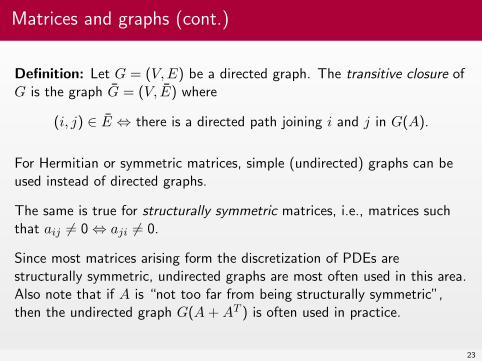
Matrices and graphs (cont.)
Definition: Let G = (V,E) be a directed graph. The transitive closure ofG is the graph G = (V, E) where
(i, j) ∈ E ⇔ there is a directed path joining i and j in G(A).
For Hermitian or symmetric matrices, simple (undirected) graphs can beused instead of directed graphs.
The same is true for structurally symmetric matrices, i.e., matrices suchthat aij 6= 0 ⇔ aji 6= 0.
Since most matrices arising form the discretization of PDEs arestructurally symmetric, undirected graphs are most often used in this area.Also note that if A is “not too far from being structurally symmetric”,then the undirected graph G(A+AT ) is often used in practice.
23

Irreducibility
Definition: A matrix A ∈ Cn×n is reducible if there exists a permutationmatrix P such that
P TAP =
[A11 A12
0 A22
]with A11 and A22 square submatrices. If no such P exists, A is said to beirreducible.
Theorem. The following statements are equivalent:(i) the matrix A is irreducible(ii) the digraph G(A) is strongly connected, i.e., for every pair of nodes i
and j in V there is a directed path in G(A) that starts at node i andends at node j
(iii) the transitive closure G(A) of G(A) is the complete graph on V , i.e.,the graph with edge set E = V × V .
Note that (iii) and the Cayley–Hamilton Theorem imply that the powers (I +A)p
are completely full for p ≥ n− 1 (barring cancellation).24
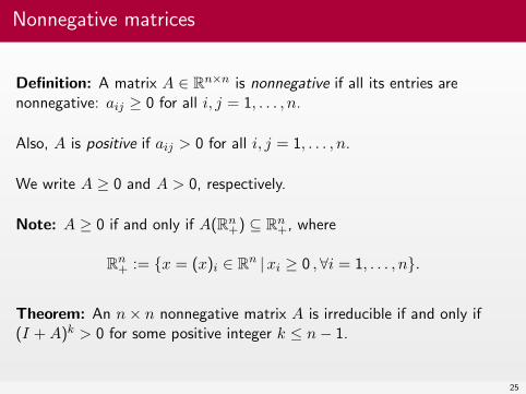
Nonnegative matrices
Definition: A matrix A ∈ Rn×n is nonnegative if all its entries arenonnegative: aij ≥ 0 for all i, j = 1, . . . , n.
Also, A is positive if aij > 0 for all i, j = 1, . . . , n.
We write A ≥ 0 and A > 0, respectively.
Note: A ≥ 0 if and only if A(Rn+) ⊆ Rn
+, where
Rn+ := x = (x)i ∈ Rn |xi ≥ 0 ,∀i = 1, . . . , n.
Theorem: An n× n nonnegative matrix A is irreducible if and only if(I +A)k > 0 for some positive integer k ≤ n− 1.
25

Nonnegative matrices (cont.)
Theorem (Perron–Frobenius): Let A ≥ 0 be irreducible, then(i) ρ(A) is a simple eigenvalue of A;(ii) There exists a positive eigenvector x = (xi) associated with ρ(A):
Ax = ρ(A)x, xi > 0 ∀i = 1, . . . , n;
(iii) ρ(A) increases when any entry of A increases; that is,
A ≥ A and A 6= A ⇒ ρ(A) > ρ(A)
Here A ≥ A means that A−A is nonnegative.
The Perron–Frobenius Theorem holds in particular for positive matrices.
26
Perron & Frobenius
Oskar Perron (1880-1975) and Georg Ferdinand Frobenius (1849-1917)
27

M -matrices
Definition: A matrix A ∈ Rn×n is an M -matrix if it can be written as
A = rI −B, where B ≥ 0 and r ≥ ρ(B).
If r > ρ(B) then A is a nonsingular M -matrix.
Theorem: A matrix A ∈ Rn×n is a nonsingular M -matrix if and only ifaij ≤ 0 for all i 6= j and A is invertible with A−1 ≥ 0.
Note: If A is an irreducible nonsingular M -matrix, then A−1 > 0.
Definition: An invertible matrix A ∈ Rn×n is monotone if A−1 ≥ 0.
Matrix monotonicity corresponds to a discrete maximum principle.All nonsingular M -matrices are monotone, but the converse is nottrue.
28

M -matrices (cont.)
Theorem: Let A ∈ Rn×n be a symmetric nonsingular M -matrix. Then Ais positive definite.
Symmetric nonsingular M -matrices are sometimes called Stieltjes matrices.
A nonsymmetric nonsingular M -matrix is not necessarily positive definite;that is, A+AT may be indefinite. A simple example is given by
A =
[1 −30 1
]
However, all nonsingular M -matrices are positive stable: Re(λ) > 0, for allλ ∈ σ(A).
M -matrices are extremely well-behaved from the numerical point of view.
29
Geršgorin’s Theorem
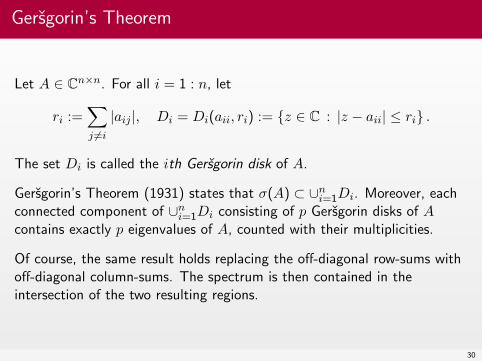
Let A ∈ Cn×n. For all i = 1 : n, let
ri :=∑j 6=i
|aij |, Di = Di(aii, ri) := z ∈ C : |z − aii| ≤ ri .
The set Di is called the ith Geršgorin disk of A.
Geršgorin’s Theorem (1931) states that σ(A) ⊂ ∪ni=1Di. Moreover, each
connected component of ∪ni=1Di consisting of p Geršgorin disks of A
contains exactly p eigenvalues of A, counted with their multiplicities.
Of course, the same result holds replacing the off-diagonal row-sums withoff-diagonal column-sums. The spectrum is then contained in theintersection of the two resulting regions.
30

The Field of Values
The field of values (or numerical range) of A ∈ Cn×n is the set
W(A) := z = 〈Ax, x〉 |x∗x = 1 .
This set is a compact subset of C containing the eigenvalues of A; it isalso convex. This last statement is known as the Hausdorff–ToeplitzTheorem, and is highly nontrivial.
The definition of numerical range also applies to bounded linear operatorson a Hilbert space H; however, W(A) may not be closed if dim (H) = ∞.
R. Horn and C. Johnson, Topics in Matrix Analysis, Cambridge UniversityPress, 1994.
31

The Field of Values (cont.)
−1 0 1 2 3 4 5 6−1.5
−1
−0.5
0
0.5
1
1.5
Field of Values of a random 10× 10 matrix.
32

Outline
1 Plan of these lectures
2 Review of matrix theory
3 Functions of matrices
4 Bibliography
33

Motivation
Both classical and new applications have resulted in increased interest inthe theory and computation of matrix functions over the past few years:
Solution of time-dependent ODEs/PDEsQuantum chemistry (electronic structure theory)Applications to Network ScienceTheoretical particle physics (QCD)Markov models in financeData miningControl theoryetc.
Currently a hot topic in scientific computing!
34

A bit of history
Simple matrix functions appear already in Cayley’s A memoir on thetheory of matrices (1858). This is considered to be “the first paper toinvestigate the algebraic properties of matrices regarded as objects ofstudy in their own right” (N. J. Higham).
The term matrix itself had been introduced by Sylvester already in 1850.
In his paper Cayley considered square roots of matrices, as well as polynomialand rational functions of a matrix (the simplest of which is, of course, A−1).The paper also contains a statement of the Cayley–Hamilton Theorem.
A. Cayley, A memoir on the theory of matrices, Phil. Trans. Roy. Soc. London,148:17–37, 1858.
35

Founding fathers
Arthur Cayley (1821-1895) and James Joseph Sylvester (1814-1897)
36
Definitions of Matrix Function
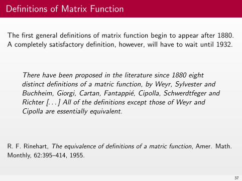
The first general definitions of matrix function begin to appear after 1880.A completely satisfactory definition, however, will have to wait until 1932.
There have been proposed in the literature since 1880 eightdistinct definitions of a matric function, by Weyr, Sylvester andBuchheim, Giorgi, Cartan, Fantappié, Cipolla, Schwerdtfeger andRichter [. . . ] All of the definitions except those of Weyr andCipolla are essentially equivalent.
R. F. Rinehart, The equivalence of definitions of a matric function, Amer. Math.Monthly, 62:395–414, 1955.
37

Matrix function as defined by Sylvester (1883) andBuchheim (1886)
Polynomial interpolationLet λ1, . . . , λs be the distinct eigenvalues of A ∈ Cn×n and let ni be theindex of λi. Then f(A) := r(A), where r is the unique Lagrange–Hermite
interpolating polynomial of degree <s∑
i=1ni satisfying
r(j)(λi) = f (j)(λi) j = 0, . . . , ni − 1, i = 1, . . . , s.
Of course, this implies that the values f (j)(λi) with 0 ≤ j ≤ ni − 1 and1 ≤ i ≤ s exist. We say that f is defined on the spectrum of A. When allthe eigenvalues are distinct, the interpolation polynomial has degree n− 1.
Remark:Every matrix function is a polynomial in A!
38

Matrix function as defined by Weyr (1887)
Taylor seriesSuppose f has a Taylor series expansion
f(z) =∞∑
k=0
ak(z − α)k
(ak =
f (k)(α)
k!
)
with radius of convergence r. If A ∈ Cn×n and each of the distincteigenvalues λ1, . . . , λs of A satisfies
|λi − α| < r,
then
f(A) :=∞∑
k=0
ak(A− αI)k.
39
Matrix function as defined by Giorgi (1928)
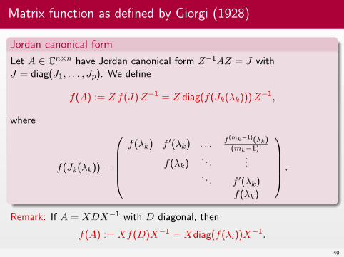
Jordan canonical formLet A ∈ Cn×n have Jordan canonical form Z−1AZ = J withJ = diag(J1, . . . , Jp). We define
f(A) := Z f(J)Z−1 = Z diag(f(Jk(λk)))Z−1,
where
f(Jk(λk)) =
f(λk) f ′(λk) . . . f (mk−1)(λk)
(mk−1)!
f(λk). . .
.... . . f ′(λk)
f(λk)
.
Remark: If A = XDX−1 with D diagonal, then
f(A) := Xf(D)X−1 = Xdiag(f(λi))X−1.
40
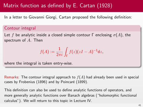
Matrix function as defined by E. Cartan (1928)
In a letter to Giovanni Giorgi, Cartan proposed the following definition:
Contour integralLet f be analytic inside a closed simple contour Γ enclosing σ(A), thespectrum of A. Then
f(A) :=1
2πi
∫Γf(z)(zI −A)−1dz,
where the integral is taken entry-wise.
Remarks: The contour integral approach to f(A) had already been used in specialcases by Frobenius (1896) and by Poincaré (1899).
This definition can also be used to define analytic functions of operators, andmore generally analytic functions over Banach algebras (“holomorphic functionalcalculus”). We will return to this topic in Lecture IV.
41
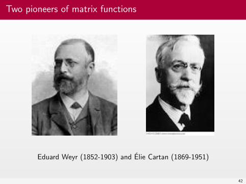
Two pioneers of matrix functions
Eduard Weyr (1852-1903) and Élie Cartan (1869-1951)
42

Primary vs. non-primary matrix functions
Giorgi’s definition assumes that whenever f is a multi-valued function(e.g., the square root or the logarithm), the same branch of f is used forevery Jordan block of A. Such matrix functions are called primary matrixfunctions.
Functions that allow using different branches of f for different Jordanblocks are called non-primary. The most general definition of a matrixfunction, due to Cipolla (1932), includes non-primary functions.
For example, [1 00 1
]and
[−1 00 −1
]are both primary square roots of I2, but[
1 00 −1
]and
[−1 00 1
]are non-primary. Here we only consider primary matrix functions.
43
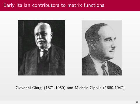
Early Italian contributors to matrix functions
Giovanni Giorgi (1871-1950) and Michele Cipolla (1880-1947)
44

Commemorative stamp of Giovanni Giorgi (1990)
Giorgi introduced a precursor of the metric system based on four units.
45

And if you are really interested...
J. J. Sylvester, On the equation to the secular inequalities in the planetary theory,Phil. Mag., 16: 267–269, 1883.
A. Buchheim, On the theory of matrices, Proc. London Math. Soc., 16:63–82,1884.
—, An extension of a theorem of Professor Sylvester’s relating to matrices,Phil. Mag., 22: 173–174, 1886. Fifth Series.
E. Weyr, Note sur la théorie des quantités complexes formées avec n unitésprincipales, Bull. Sci. Math. II, 11:205–215, 1887.
G. Giorgi, Nuove osservazioni sulle funzioni delle matrici, Atti Accad. LinceiRend., 6(8):3–8, 1928.
M. Cipolla, Sulle matrici espressioni analitiche di un’altra, Rend. CircoloMatematico Palermo, 56:144–154, 1932.
46
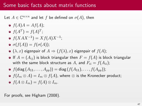
Some basic facts about matrix functions
Let A ∈ Cn×n and let f be defined on σ(A), then
f(A)A = Af(A);f(AT ) = f(A)T ;f(XAX−1) = Xf(A)X−1;σ(f(A)) = f(σ(A));(λ, x) eigenpair of A ⇒ (f(λ), x) eigenpair of f(A);If A = (Aij) is block triangular then F = f(A) is block triangularwith the same block structure as A, and Fii = f(Aii);f(diag (A11, . . . , App)) = diag (f(A11), . . . , f(App));f(Im ⊗A) = Im ⊗ f(A), where ⊗ is the Kronecker product;f(A⊗ Im) = f(A)⊗ Im.
For proofs, see Higham (2008).
47
Some basic facts about matrix functions (cont.)
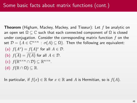
Theorem (Higham, Mackey, Mackey, and Tisseur): Let f be analytic onan open set Ω ⊆ C such that each connected component of Ω is closedunder conjugation. Consider the corresponding matrix function f on theset D = A ∈ Cn×n : σ(A) ⊆ Ω. Then the following are equivalent:(a) f(A∗) = f(A)∗ for all A ∈ D.(b) f(A) = f(A) for all A ∈ D.(c) f(Rn×n ∩ D) ⊆ Rn×n.(d) f(R ∩ Ω) ⊆ R.
In particular, if f(x) ∈ R for x ∈ R and A is Hermitian, so is f(A).
48

Some basic facts about matrix functions (cont.)
Let A ∈ Cn×n and let f be defined on σ(A). The following expressions (inincreasing order of generality) are often useful:
If A is normal (in particular, Hermitian) then
f(A) =n∑
i=1
f(λi)uiu∗i
If A ∈ Cn×n is diagonalizable then
f(A) =n∑
i=1
f(λi)xiy∗i
If A is arbitrary then
f(A) =s∑
i=1
ni−1∑j=0
f (j)(λi)
j!(A− λiI)
jGi
49
Some basic facts about matrix functions (cont.)
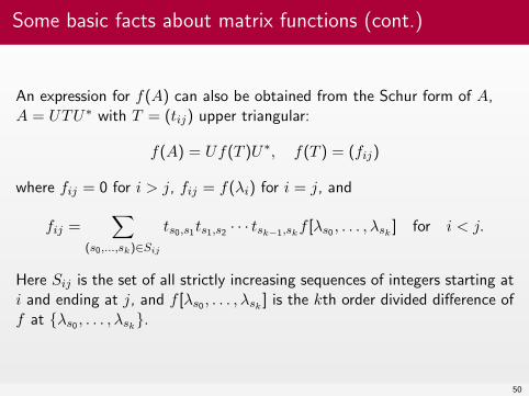
An expression for f(A) can also be obtained from the Schur form of A,A = UTU∗ with T = (tij) upper triangular:
f(A) = Uf(T )U∗, f(T ) = (fij)
where fij = 0 for i > j, fij = f(λi) for i = j, and
fij =∑
(s0,...,sk)∈Sij
ts0,s1ts1,s2 · · · tsk−1,skf [λs0 , . . . , λsk
] for i < j.
Here Sij is the set of all strictly increasing sequences of integers starting ati and ending at j, and f [λs0 , . . . , λsk
] is the kth order divided difference off at λs0 , . . . , λsk
.
50

Important examples
Let A ∈ Cn×n, and let z /∈ σ(A). The resolvent of A at z is defined as
R(A; z) = (zI −A)−1.
The resolvent is central to the definition of matrix functions via thecontour integral approach. As a special case, the resolvent can be used todefine the spectral projector onto the eigenspace of a matrix or operatorcorresponding to an isolated eigenvalue λ0 ∈ σ(A):
Pλ0 :=1
2πi
∫|z−λ0|=ε
(zI −A)−1dz
where ε > 0 is small enough so that no other eigenvalue of A falls within εof λ0.
Remarks: More generally, one can define the spectral projector onto the invariantsubspace of A corresponding to a set of selected eigenvalues by integratingR(A; z) along a countour surrounding those eigenvalues and excluding the others.
The spectral projector is orthogonal if and only if A is normal.51

Important examples (cont.)
Also extremely important is the matrix exponential
eA = I +A+1
2!A2 +
1
3!A3 + · · · =
∞∑k=0
1
k!Ak
which is defined for arbitrary A ∈ Cn×n.Just as the resolvent is central to spectral theory, the matrix exponential isfundamental to the solution of differential equations. For example, the solutionto the inhomogeneous system
dydt
= Ay + f(t, y), y(0) = y0, y ∈ Cn, A ∈ Cn×n
is given (implicitly!) by
y(t) = etAy0 +
∫ t
0
eA(t−s)f(s, y(s))ds.
In particular, y(t) = etAy0 when f = 0.It is important to recall that limt→∞ etA = 0 if and only if A is a stable matrix:Re(λ) < 0, for all λ ∈ σ(A).
52

Important examples (cont.)
When f(t, y) = b ∈ Cn (=const.), the solution can also be expressed as
y(t) = tψ1(tA)(b+Ay0) + y0
where
ψ1(z) =ez − 1
z= 1 +
z
2!+z2
3!+ · · ·
Trigonometric functions and square roots of matrices are also important inapplications. For example, the solution to the second-order system
d2y
dt2+Ay = 0, y(0) = y0, y′(0) = y′0
(where A is SPD) can be expressed as
y(t) = cos(√At) y0 + (
√A)−1 sin(
√At) y′0 .
53

Important examples (cont.)
If A,B ∈ Cn×n commute (AB = BA), then the identity
eA+B = eAeB
holds true, but in general eA+B 6= eAeB.
A useful identity that is always true is
eA = cosh(A) + sinh(A) ,
where
cosh(A) =eA + e−A
2=
∞∑k=0
1
(2k)!A2k
and
sinh(A) =eA − e−A
2=
∞∑k=0
1
(2k + 1)!A2k+1 .
54

Important examples (cont.)
Apart from the contour integration formula, the matrix exponential andthe resolvent are also related through the Laplace transform: there existsan ω ∈ R such that z /∈ σ(A) for Re(z) > ω and
(zI −A)−1 =
∫ ∞
0e−ztetAdt =
∫ ∞
0e−t(zI−A)dt .
Recall also that if |z| > ρ(A), the following Neumann series expansion ofthe resolvent is valid:
(zI −A)−1 = z−1(I + z−1A+ z−2A2 + · · · ) = z−1∞∑
k=0
z−kAk.
A useful variant of this expression is
(I − αA)−1 = I + αA+ α2A2 + · · · =∞∑
k=0
αkAk ,
where 0 < α < 1ρ(A) .
55

Outline
1 Plan of these lectures
2 Review of matrix theory
3 Functions of matrices
4 Bibliography
56

Bibliography
F. R. Gantmacher, The Theory of Matrices, Chelsea, New York, 2 Volls., 1959.
N. J. Higham, Functions of Matrices. Theory and Computation, SIAM,Philadelphia, 2008.
R. A. Horn and C. R. Johnson, Matrix Analysis, Cambridge University Press, 1991.
R. A. Horn and C. R. Johnson, Topics in Matrix Analysis, Cambridge UniversityPress, 1994.
C. D. Meyer, Matrix Analysis and Applied Linear Algebra, SIAM, Philadelphia,2000.
L. Salce, Lezioni sulle Matrici, Decibel/Zanichelli, Padova/Bologna, 1993.
57