FUNCTIONS PRESERVING MATRIX GROUPS AND ITERATIONSFOR THE MATRIX SQUARE ROOT∗

NICHOLAS J. HIGHAM† , D. STEVEN MACKEY‡ , NILOUFER MACKEY§ , AND

FRANCOISE TISSEUR¶

Abstract. For which functions f does A ∈ G ⇒ f(A) ∈ G when G is the matrix automorphismgroup associated with a bilinear or sesquilinear form? For example, if A is symplectic when is f(A)symplectic? We show that group structure is preserved precisely when f(A−1) = f(A)−1 for bilinearforms and when f(A−∗) = f(A)−∗ for sesquilinear forms. Meromorphic functions that satisfy each

of these conditions are characterized. Related to structure preservation is the condition f(A) = f(A),and analytic functions and rational functions satisfying this condition are also characterized. Theseresults enable us to characterize all meromorphic functions that map every G into itself as the ratioof a polynomial and its “reversal”, up to a monomial factor and conjugation.

The principal square root is an important example of a function that preserves every automor-phism group G. By exploiting the matrix sign function, a new family of coupled iterations for thematrix square root is derived. Some of these iterations preserve every G; all of them are shown, viaa novel Frechet derivative-based analysis, to be numerically stable.

A rewritten form of Newton’s method for the square root of A ∈ G is also derived. Unlike theoriginal method, this new form has good numerical stability properties, and we argue that it is theiterative method of choice for computing A1/2 when A ∈ G. Our tools include a formula for thesign of a certain block 2 × 2 matrix, the generalized polar decomposition along with a wide class ofiterations for computing it, and a connection between the generalized polar decomposition of I + A

and the square root of A ∈ G.

Key words. automorphism group, bilinear form, sesquilinear form, scalar product, adjoint,Frechet derivative, stability analysis, perplectic matrix, pseudo-orthogonal matrix, Lorentz group,generalized polar decomposition, matrix sign function, matrix pth root, matrix square root, structurepreservation, matrix iteration, Newton iteration

AMS subject classifications. 65F30, 15A18

1. Introduction. Theory and algorithms for structured matrices are of growinginterest because of the many applications that generate structure and the potentialbenefits to be gained by exploiting it. The benefits include faster and more accuratealgorithms as well as more physically meaningful solutions. Structure comes in manyforms, including Hamiltonian, Toeplitz or Vandermonde structure and total positivity.Here we study a nonlinear structure that arises in a variety of important applicationsand has an elegant mathematical formulation: that of a matrix automorphism groupG associated with a bilinear or sesquilinear form.

Our particular interest is in functions that preserve matrix automorphism groupstructure. We show in Section 3 that A ∈ G ⇒ f(A) ∈ G precisely when f(A−1) =

∗Numerical Analysis Report 446, Manchester Centre for Computational Mathematics, June 2004.†Department of Mathematics, University of Manchester, Manchester, M13 9PL, England

(higham@ma.man.ac.uk, http://www.ma.man.ac.uk/~higham/). This work was supported by Engi-neering and Physical Sciences Research Council grant GR/R22612 and by a Royal Society-WolfsonResearch Merit Award.

‡Department of Mathematics, University of Manchester, Manchester, M13 9PL, England(smackey@ma.man.ac.uk). This work was supported by Engineering and Physical Sciences ResearchCouncil grant GR/S31693.

§Department of Mathematics, Western Michigan University, Kalamazoo, MI 49008, USA(nil.mackey@wmich.edu, http://homepages.wmich.edu/~mackey/).

¶Department of Mathematics, University of Manchester, Manchester, M13 9PL, England(ftisseur@ma.man.ac.uk, http://www.ma.man.ac.uk/~ftisseur/). This work was supported by En-gineering and Physical Sciences Research Council grant GR/R45079.

1

f(A)−1 for bilinear forms or f(A−∗) = f(A)−∗ for sesquilinear forms; in other words,f has to commute with the inverse function or the conjugate inverse function atA. We characterize meromorphic functions satisfying each of these conditions. Forsesquilinear forms, the condition f(A) = f(A), that is, f commutes with conjugation,also plays a role in structure preservation. We characterize analytic functions andrational functions satisfying this conjugation condition. We show further that anymeromorphic function that is structure preserving for all automorphism groups isrational and, up to a monomial factor and conjugation, the ratio of a polynomial andits “reversal”.

The matrix sign function and the matrix principal pth root are important exam-ples of functions that preserve all automorphism groups. Iterations for computing thesign function in a matrix group were studied by us in [15]. We concentrate here onthe square root, aiming to derive iterations that exploit the group structure. Connec-tions between the matrix sign function, the matrix square root, and the generalizedpolar decomposition are developed in Section 4. A new identity for the matrix signfunction (Lemma 4.3) establishes a link with the generalized polar decomposition(Corollary 4.4). For A ∈ G we show that the generalized polar decomposition ofI + A has A1/2 as the factor in G, thereby reducing computation of the square rootto computation of the generalized polar decomposition (Theorem 4.7).

A great deal is known about iterations for the matrix sign function. Our resultsin Section 4 show that each matrix sign function iteration of a general form leads totwo further iterations:

• A coupled iteration for the principal square root of any matrix A. The iter-ation is structure preserving, in the sense that A ∈ G implies all the iterateslie in G, as long as the underlying sign iteration is also structure preserving.

• An iteration for the generalized polar decomposition, and hence for the squareroot of A ∈ G.

Iterations for matrix roots are notorious for their tendency to be numericallyunstable. In Section 5 Frechet derivatives are used to develop a stability analysisof the coupled square root iterations that arise from superlinearly convergent signiterations. We find that all such iterations are stable, but that a seemingly innocuousrewriting of the iterations can make them unstable. The technique developed in thissection should prove to be of wider use in analyzing matrix iterations.

In Section 6 two instances of the connections identified in Section 4 betweenthe sign function and the square root are examined in detail. We obtain a familyof coupled structure-preserving iterations for the square root whose members haveorder of convergence 2m + 1 for m = 1, 2, . . .. We also derive a variant for A ∈ G

of the well-known but numerically unstable Newton iteration for A1/2 by using theconnection with the generalized polar decomposition. Our numerical experiments andanalysis in Section 7 confirm the numerical stability of both the structure-preservingiterations and the Newton variant, showing both to be useful in practice. Because theNewton variant has a lower cost per iteration and shows better numerical preservationof structure, it is our preferred method in general.

2. Preliminaries. We give a very brief summary of the required definitions andnotation. For more details, see Mackey, Mackey, and Tisseur [25].

Consider a scalar product on Kn, that is, a bilinear or sesquilinear form 〈·, ·〉

M

defined by any nonsingular matrix M : for x, y ∈ Kn,

〈x, y〉M

=

xT My, for real or complex bilinear forms,x∗My, for sesquilinear forms.

2

Here K = R or C and the superscript ∗ denotes conjugate transpose. The associatedautomorphism group is defined by

G = A ∈ Kn×n : 〈Ax,Ay〉

M= 〈x, y〉

M, ∀x, y ∈ K

n .

The adjoint A⋆ of A ∈ Kn×n with respect to 〈·, ·〉

Mis the unique matrix satisfying

〈Ax, y〉M

= 〈x,A⋆y〉M

∀x, y ∈ Kn.

It can be shown that the adjoint is given explicitly by

A⋆ =

M−1AT M, for bilinear forms,M−1A∗M, for sesquilinear forms

(2.1)

and has the following basic properties:

(A + B)⋆ = A⋆ + B⋆, (AB)⋆ = B⋆A⋆, (A−1)⋆ = (A⋆)−1,

(αA)⋆ =

αA⋆, for bilinear forms,αA⋆, for sesquilinear forms.

The automorphism group can be characterized in terms of the adjoint by

G = A ∈ Kn×n : A⋆ = A−1 .

Table 2.1 lists some of the “classical” matrix groups. Observe that M , the matrixof the form, is real orthogonal with M = ±MT in all these examples. Our results,however, place no restrictions on M other than nonsingularity; they therefore applyto all scalar products on R

n or Cn and their associated automorphism groups.

We note for later use that

A ∈ G and M unitary ⇒ ‖A‖2 = ‖A−1‖2.(2.2)

We recall one of several equivalent ways of defining f(A) for A ∈ Cn×n, where f is

an underlying scalar function. Let A have distinct eigenvalues λ1, . . . , λs occurring inJordan blocks of maximum sizes n1, . . . , ns, respectively. Thus if A is diagonalizable,ni ≡ 1. Then f(A) = q(A), where q is the unique Hermite interpolating polynomialof degree less than

∑si=1 ni that satisfies the interpolation conditions

q(j)(λi) = f (j)(λi), j = 0:ni − 1, i = 1: s.(2.3)

Stated another way, q is the Hermite interpolating polynomial of minimal degree thatinterpolates f at the roots of the minimal polynomial of A. We use the phrase f is

defined on the spectrum of A or, for short, f is defined at A or A is in the domain of

f , to mean that the derivatives in (2.3) exist.At various points in this work the properties f

(diag(X1,X2)

)= diag(f(X1), f(X2))

and f(P−1AP ) = P−1f(A)P , which hold for any matrix function [24, Thms. 9.4.1,9.4.2], will be used. We will also need the following three results.

Lemma 2.1. Let A,B ∈ Cn×n and let f be defined on the spectrum of both A and

B. Then there is a single polynomial p such that f(A) = p(A) and f(B) = p(B).Proof. It suffices to let p be the polynomial that interpolates f and its derivatives

at the roots of the least common multiple of the minimal polynomials of A and B.See the discussion in [16, p. 415].

3

Table 2.1A sampling of automorphism groups.

Here, R =

[1

. ..

1

], J =

[0 In

−In 0

], Σp,q =

[Ip 00 −Iq

]∈ Rn×n.

Space M A⋆ Automorphism group, G

Groups corresponding to a bilinear form

Rn I A⋆ = AT Real orthogonals

Cn I A⋆ = AT Complex orthogonals

Rn Σp,q A⋆ = Σp,qAT Σp,q Pseudo-orthogonalsa

Rn R A⋆ = RAT R Real perplectics

R2n J A⋆ = −JAT J Real symplectics

C2n J A⋆ = −JAT J Complex symplectics

Groups corresponding to a sesquilinear form

Cn I A⋆ = A∗ Unitaries

Cn Σp,q A⋆ = Σp,qA∗Σp,q Pseudo-unitaries

C2n J A⋆ = −JA∗J Conjugate symplectics

aAlso known as the Lorentz group.

Corollary 2.2. Let A,B ∈ Cn×n and let f be defined on the spectra of both

AB and BA. Then

Af(BA) = f(AB)A.

Proof. By Lemma 2.1 there is a single polynomial p such that f(AB) = p(AB)and f(BA) = p(BA). Hence

Af(BA) = Ap(BA) = p(AB)A = f(AB)A.

Lemma 2.3. Any rational function r can be uniquely represented in the form

r(z) = znp(z)/q(z), where p is monic, n is an integer, p and q are relatively prime,

and p(0) and q(0) are both nonzero.

Proof. Straightforward.

We denote the closed negative real axis by R−. For A ∈ C

n×n with no eigenvalueson R

−, the principal matrix pth root A1/p is defined by the property that the eigen-values of A1/p lie in the segment z : −π/p < arg(z) < π/p . We will most often usethe principal square root, A1/2, whose eigenvalues lie in the open right half-plane.

Finally, we introduce some notation connected with a polynomial p. The polyno-mial obtained by replacing the coefficients of p by their conjugates is denoted by p.The polynomial obtained by reversing the order of the coefficients of p is denoted byrevp; thus if p has degree m then

revp(x) = xmp(1/x).(2.4)

3. Structure-preserving functions. Our aim in this section is to characterizefunctions f that preserve automorphism group structure. For a given G, if f(A) ∈ G

for all A ∈ G for which f(A) is defined, we will say that f is structure preserving for

G. As well as determining f that preserve structure for a particular G, we wish todetermine f that preserve structure for all G.

4

The (principal) square root is an important example of a function that preservesall groups. To see this for G associated with a bilinear form, recall that A ∈ G isequivalent to M−1AT M = A−1. Assuming that A has no eigenvalues on R

−, takingthe (principal) square root in this relation gives

A−1/2 = (M−1AT M)1/2 = M−1(AT

)1/2M = M−1

(A1/2

)TM,(3.1)

which shows that A1/2 ∈ G.In order to understand structure preservation we need first to characterize when

f(A) ∈ G for a fixed f and a fixed A ∈ G. The next result relates this property tovarious other relevant properties of matrix functions.

Theorem 3.1. Let G be the automorphism group of a scalar product. Consider

the following eight properties of a matrix function f at a (fixed) matrix A ∈ Kn×n,

where f is assumed to be defined at the indicated arguments:(a) f(AT ) = f(A)T , (e) f(A−1) = f(A)−1,

(b) f(A∗) = f(A)∗, (g) f(A−∗) = f(A)−∗,

(c) f(A) = f(A), (h) f(A−⋆) = f(A)−⋆,

(d) f(A⋆) = f(A)⋆, (i) when A ∈ G, f(A) ∈ G.

(a) always holds. (b) is equivalent to (c). (c) is equivalent to the existence of a single

real polynomial p such that f(A) = p(A) and f(A) = p(A). Any two of (d), (e) and

(h) imply the third1. Moreover,

• for bilinear forms: (d) always holds. (e), (h) and (i) are equivalent;

• for sesquilinear forms: (d) is equivalent to (b) and to (c). (g), (h) and (i)are equivalent.

Proof. (a) follows because the same polynomial can be used to evaluate f(A)

and f(AT ), by Lemma 2.1. Property (b) is equivalent to f(AT) = f(A)

T, which on

applying (a) becomes (c). So (b) is equivalent to (c).Next, we consider the characterization of (c). Suppose p is a real polynomial such

that f(A) = p(A) and f(A) = p(A). Then f(A) = p(A) = p(A) = f(A), which is (c).Conversely, assume (c) holds and let q be any complex polynomial that simultaneouslyevaluates f at A and A, so that f(A) = q(A) and f(A) = q(A); the existence of sucha q is assured by Lemma 2.1. Then

q(A) = f(A) = f(A) = q(A) = q(A),

and hence p(x) := 12 (q(x) + q(x)) is a real polynomial such that f(A) = p(A). Since

q(A) = f(A) = f(A) = q(A) = q(A),

we also have f(A) = p(A).We now consider (d). From the characterization (2.1) of the adjoint, for bilinear

forms we have

f(A⋆) = f(M−1AT M) = M−1f(AT )M = M−1f(A)T M = f(A)⋆,

so (d) always holds. For sesquilinear forms,

f(A⋆) = f(M−1A∗M) = M−1f(A∗)M,

1We will see at the end of Section 3.4 that for sesquilinear forms neither (d) nor (e) is a necessarycondition for (h) (or, equivalently, for the structure-preservation property (i)).

5

which equals f(A)⋆ = M−1f(A)∗M if and only if (b) holds. It is straightforward toshow that any two of (d), (e) and (h) imply the third.

To see that (h) and (i) are equivalent, consider the following cycle of potentialequalities:

f(A−⋆)(h)

== f(A)−⋆

(x) \\ \\(y)

f(A)

Clearly (x) holds if A ∈ G, and (y) holds when f(A) ∈ G. Hence (h) and (i) areequivalent.

For bilinear forms,

f(A−⋆) = f(A)−⋆ ⇐⇒ f(M−1A−T M) = M−1f(A)−T M

⇐⇒ f(A−T ) = f(A)−T

⇐⇒ f(A−1) = f(A)−1 by (a).

Thus (h) is equivalent to (e). For sesquilinear forms a similar argument shows that(h) is equivalent to (g).

The main conclusion of Theorem 3.1 is that f is structure preserving for G pre-cisely when f(A−1) = f(A)−1 for all A ∈ G for bilinear forms, or f(A−∗) = f(A)−∗

for all A ∈ G for sesquilinear forms. We can readily identify two important functionsthat satisfy both these conditions more generally for all A ∈ K

n×n in their domains,and hence are structure preserving for all G.

• The matrix sign function. Recall that for a matrix A ∈ Cn×n with no

pure imaginary eigenvalues the sign function can be defined by sign(A) =A(A2)−1/2 [12], [22]. That the sign function is structure preserving is known:proofs specific to the sign function are given in [15] and [26].

• Any matrix power Aα, subject for fractional α to suitable choice of thebranches of the power at each eigenvalue; in particular, the principal ma-trix pth root A1/p. The structure-preserving property of the principal square

root is also shown by Mackey, Mackey, and Tisseur [26].In the following three subsections we investigate three of the properties in Theo-

rem 3.1 in detail, for general matrices A ∈ Cn×n. Then in the final two subsections

we characterize meromorphic structure-preserving functions and conclude with a briefconsideration of M -normal matrices.

3.1. Property (c): f(A) = f(A). Theorem 3.1 shows that this property, to-gether with property (e), namely f(A−1) = f(A)−1, is sufficient for structure preser-vation in the sesquilinear case. While property (c) is not necessary for structurepreservation, it plays an important role in our understanding of the preservation ofrealness, and so is of independent interest.

We first give a characterization of analytic functions satisfying property (c) forall A in their domain, followed by an explicit description of all rational functions withthe property. We denote by Λ(A) the set of eigenvalues of A.

Theorem 3.2. Let f be analytic on an open subset Ω ⊆ C such that each

connected component of Ω is closed under conjugation. Consider the corresponding

matrix function f on its natural domain in Cn×n, the set D = A ∈ C

n×n : Λ(A) ⊆Ω . Then the following are equivalent:

6

(a) f(A) = f(A) for all A ∈ D.

(b) f(Rn×n ∩ D) ⊆ Rn×n.

(c) f(R ∩ Ω) ⊆ R.

Proof. Our strategy is to show that (a) ⇒ (b) ⇒ (c) ⇒ (a).(a) ⇒ (b): If A ∈ R

n×n ∩ D then

f(A) = f(A) (since A ∈ Rn×n)

= f(A) (given),

so f(A) ∈ Rn×n, as required.

(b) ⇒ (c): If λ ∈ R∩Ω then λI ∈ D. But f(λI) ∈ Rn×n by (b), and hence, since

f(λI) = f(λ)I, f(λ) ∈ R.

(c) ⇒ (a): Let Ω be any connected component of Ω. Since Ω is open andconnected it is path-connected, and since it is also closed under conjugation it mustcontain some λ ∈ R by the intermediate value theorem. The openness of Ω in C

then implies that U = Ω ∩ R is a nonempty open subset of R, with f(U) ⊆ R by

hypothesis. Now since f is analytic on Ω, it follows from the “identity theorem” [27,

pp. 227–236 and Ex. 4, p. 236] that f(z) = f(z) for all z ∈ Ω. The same argumentapplies to all the other connected components of Ω, so f(z) = f(z) for all z ∈ Ω. Thusf(A) = f(A) holds for all diagonal matrices in D, and hence for all diagonalizablematrices in D. Since the scalar function f is analytic on Ω, the matrix function f iscontinuous on D [16, Thm. 6.2.27]2 and therefore the identity holds for all matricesin D, since diagonalizable matrices are dense in any open subset of C

n×n.

Turning to the case when f is rational, we need a preliminary lemma.Lemma 3.3. Suppose r is a complex rational function that maps all reals (in its

domain) to reals. Then r can be expressed as the ratio of two real polynomials. In

particular, in the canonical form for r given by Lemma 2.3 the polynomials p and qare both real.

Proof. Let r(z) = znp(z)/q(z) be the canonical form of Lemma 2.3 and considerthe rational function

h(z) := r(z) = zn p(z)

q(z).

Clearly, h(z) = r(z) for all real z in the domain of r, and hence p(z)/q(z) = p(z)/q(z)for this infinitude of z. It is then straightforward to show (cf. the proof of Lemma 3.6below) that p = αp and q = αq for some nonzero α ∈ C. But the monicity of p impliesthat α = 1, so p and q are real polynomials.

Combining Lemma 3.3 with Theorem 3.2 gives a characterization of all rationalmatrix functions with property (c) in Theorem 3.1.

Theorem 3.4. A rational matrix function r(A) has the property r(A) = r(A)for all A ∈ C

n×n such that A and A are in the domain of r if and only if the scalar

function r can be expressed as the ratio of two real polynomials. In particular, the

polynomials p satisfying p(A) = p(A) for all A ∈ Cn×n are precisely those with real

coefficients.

2Horn and Johnson require that Ω should be a simply-connected open subset of C. However, itis not difficult to show that just the openness of Ω is sufficient to conclude that the matrix functionf is continuous on D.

7

3.2. Property (e): f(A−1) = f(A)−1. We now investigate further the prop-erty f(A−1) = f(A)−1 for matrix functions f . We would like to know when this prop-erty holds for all A such that A and A−1 are in the domain of f . Since a function of adiagonal matrix is diagonal, a necessary condition on f is that f(z)f(1/z) = 1 when-ever z and 1/z are in the domain of f . The following result characterizes meromorphicfunctions satisfying this identity. Recall that a function is said to be meromorphic onan open subset U ⊆ C if it is analytic on U except for poles. In this paper we onlyconsider meromorphic functions on C, so the phrase “f is meromorphic” will mean fis meromorphic on C.

Lemma 3.5. Suppose f is a meromorphic function on C such that f(z)f(1/z) = 1holds for all z in some infinite compact subset of C. Then

(a) The identity f(z)f(1/z) = 1 holds for all nonzero z ∈ C \ S, where S is the

discrete set consisting of the zeros and poles of f together with their reciprocals.

(b) The zeros and poles of f come in reciprocal pairs a, 1/a with matching

orders. That is,

z = a is a zero (pole) of order k ⇐⇒ z = 1/a is a pole (zero) of order k.(3.2)

Consequently, the set S is finite and consists of just the zeros and poles of f . Note that

0,∞ is also to be regarded as a reciprocal pair for the purpose of statement (3.2).(c) The function f is meromorphic at ∞.

(d) The function f is rational.

Proof. (a) The function g(z) := f(z)f(1/z) is analytic on the open connected setC \ S ∪ 0, so the result follows by the identity theorem.

(b) Consider first the case where a 6= 0 is a zero or a pole of f . Because f ismeromorphic the set S is discrete, so by (a) there is some open neighborhood U ofz = a such that f(z)f(1/z) = 1 holds for all z ∈ U \ a and such that f can beexpressed as f(z) = (z − a)kg(z) for some nonzero k ∈ Z (k > 0 for a zero, k < 0 fora pole) and some function g that is analytic and nonzero on all of U . Then for allz ∈ U \ a we have

f(1/z) =1

f(z)= (z − a)−k 1

g(z).

Letting w = 1/z, we see that there is an open neighborhood U of w = 1/a in which

f(w) =

(1

w− a

)−k

1

g(1/w)=

(w − 1

a

)−k

(−1)kwk

akg(1/w)=:

(w − 1

a

)−k

h(w)

holds for all w ∈ U \ 1a, where h(w) is analytic and nonzero for all w ∈ U . This

establishes (3.2), and hence that the set S consists of just the zeros and poles of f .Next we turn to the case of the “reciprocal” pair 0,∞. First note that the zeros

and poles of any nonzero meromorphic function can never accumulate at any finitepoint z, so in particular z = 0 cannot be a limit point of S. In our situation the setS also cannot have z = ∞ as an accumulation point; if it did, then the reciprocalpairing of the nonzero poles and zeros of f just established would force z = 0 to bea limit point of S. Thus if z = ∞ is a zero or singularity of f then it must be anisolated zero or singularity, which implies that S is a finite set.

Now suppose z = 0 is a zero or pole of f . In some open neighborhood U of z = 0we can write f(z) = zkg(z) for some nonzero k ∈ Z and some g that is analytic and

8

nonzero on U . Then for all z ∈ U \ 0 we have

f(1/z) =1

f(z)= z−k 1

g(z)=: z−kh(z),

where h is analytic and nonzero in U . Thus z = 0 being a zero (pole) of f impliesthat z = ∞ is a pole (zero) of f . The converse is established by the same kind ofargument.

(c) That f is meromorphic at ∞ follows from (3.2), the finiteness of S, and theidentity f(z)f(1/z) = 1, together with the fact that f (being meromorphic on C) canhave only a pole, a zero, or a finite value at z = 0.

(d) By [9, Thm. 4.7.7] a function is meromorphic on C and at ∞ if and only if itis rational.

Since Lemma 3.5 focuses attention on rational functions, we next give a completedescription of all rational functions satisfying the identity f(z)f(1/z) = 1. Recallthat revp is defined by (2.4).

Lemma 3.6. A complex rational function r(z) satisfies the identity r(z)r(1/z) = 1for infinitely many z ∈ C if and only if it can be expressed in the form

r(z) = ±zk p(z)

revp(z)(3.3)

for some k ∈ Z and some polynomial p. For any r of the form (3.3) the identity

r(z)r(1/z) = 1 holds for all nonzero z ∈ C except for the zeros of p and their recip-

rocals. Furthermore, there is always a unique choice of p in (3.3) so that p is monic,

p and revp are relatively prime, and p(0) 6= 0; in this case the sign is also uniquely

determined. In addition, r(z) is real whenever z is real if and only if this unique p is

real.

Proof. For any r of the form (3.3) it is easy to check that r(1/z) = ±z−k(revp(z))/p(z),so that the identity r(z)r(1/z) = 1 clearly holds for all nonzero z ∈ C except for thezeros of p and their reciprocals (which are the zeros of revp).

Conversely, suppose that r(z) satisfies r(z)r(1/z) = 1 for infinitely many z ∈ C.By Lemma 2.3, we can uniquely write r as r(z) = zkp(z)/q(z), where p and q arerelatively prime, p is monic, and p(0) and q(0) are both nonzero. For this uniquerepresentation of r, we will show that q(z) = ±revp(z), giving us the form (3.3).Begin by rewriting the condition r(z)r(1/z) = 1 as

p(z)p(1/z) = q(z)q(1/z).(3.4)

Letting n be any integer larger than deg p and deg q (where deg p denotes the degreeof p), multiplying both sides of (3.4) by zn and using the definition of rev results in

zn−deg pp(z)revp(z) = zn−deg qq(z)revq(z).

Since this equality of polynomials holds for infinitely many z, it must be an identity.Thus deg p = deg q, and

p(z)revp(z) = q(z)revq(z)(3.5)

holds for all z ∈ C. Since p has no factors in common with q, p must divide revq.Therefore revq(z) = αp(z) for some α ∈ C, which implies q(z) = αrevp(z) since

9

q(0) 6= 0. Substituting into (3.5) gives α2 = 1, so that q(z) = ±revp(z), as desired.The final claim follows from Lemma 3.3.

Lemmas 3.5 and 3.6 now lead us to the following characterization of meromorphicmatrix functions with the property f(A−1) = f(A)−1. Here and in the rest of thispaper we use the phrase “meromorphic matrix function f(A)” to mean a matrixfunction whose underlying scalar function f is meromorphic on all of C.

Theorem 3.7. A meromorphic matrix function f(A) has the property f(A−1) =f(A)−1 for all A ∈ C

n×n such that A and A−1 are in the domain of f if and only if

the scalar function f is rational and can be expressed in the form

f(z) = ±zk p(z)

revp(z)(3.6)

for some k ∈ Z and some polynomial p. If desired, the polynomial p may be chosen

(uniquely) so that p is monic, p and revp are relatively prime, and p(0) 6= 0. The

matrix function f(A) maps real matrices to real matrices if and only if this unique pis real.

Proof. As noted at the start of this subsection, f(z)f(1/z) = 1 for all z suchthat z and 1/z are in the domain of f is a necessary condition for having the prop-erty f(A−1) = f(A)−1. That f is rational then follows from Lemma 3.5, and fromLemma 3.6 we see that f must be of the form (3.6). To prove sufficiency, considerany f of the form (3.6) with deg p = n. Then we have

f(A)f(A−1) = ±Akp(A)[revp(A)]−1 · ±A−kp(A−1)[revp(A−1)]−1

= Akp(A)[Anp(A−1)]−1 · A−kp(A−1)[A−np(A)]−1

= Akp(A)p(A−1)−1A−n · A−kp(A−1)p(A)−1An

= I.

The final claim follows from Theorem 3.2 and Lemma 3.6.

3.3. Property (g): f(A−∗) = f(A)−∗. The results in this section provide acharacterization of meromorphic matrix functions satisfying f(A−∗) = f(A)−∗. Con-sideration of the action of f on diagonal matrices leads to the identity f(z)f(1/z) = 1as a necessary condition on f . Thus the analysis of this identity is a prerequisite forunderstanding the corresponding matrix function property.

The following analogue of Lemma 3.5 can be derived, with a similar proof.Lemma 3.8. Suppose f is a meromorphic function on C such that f(z)f(1/z) = 1

holds for all z in some infinite compact subset of C. Then f is a rational function

with its zeros and poles matched in conjugate reciprocal pairs a, 1/a. That is,

z = a is a zero (pole) of order k ⇐⇒ z = 1/a is a pole (zero) of order k,(3.7)

where 0,∞ is also to be regarded as a conjugate reciprocal pair.

In view of this result we can restrict our attention to rational functions.Lemma 3.9. A complex rational function r(z) satisfies the identity r(z)r(1/z) = 1

for infinitely many z ∈ C if and only if it can be expressed in the form

r(z) = αzk p(z)

revp(z)(3.8)

10

for some k ∈ Z, some |α| = 1, and some polynomial p. For any r of the form (3.8)the identity r(z)r(1/z) = 1 holds for all nonzero z ∈ C except for the zeros of p and

their conjugate reciprocals. Furthermore, there is always a unique choice of p in (3.8)so that p is monic, p and revp are relatively prime, and p(0) 6= 0; in this case the

scalar α is also unique. In addition, r(z) is real whenever z is real if and only if this

unique p is real and α = ±1.

Proof. The proof is entirely analogous to that of Lemma 3.6 and so is omitted.

With Lemmas 3.8 and 3.9 we can now establish the following characterization ofmeromorphic functions with the property f(A−∗) = f(A)−∗.

Theorem 3.10. A meromorphic matrix function f(A) has the property f(A−∗) =f(A)−∗ for all A ∈ C

n×n such that A and A−∗ are in the domain of f if and only if

the scalar function f is rational and can be expressed in the form

f(z) = αzk p(z)

revp(z)(3.9)

for some k ∈ Z, some |α| = 1, and some polynomial p. If desired, the polynomial pmay be chosen (uniquely) so that p is monic, p and revp are relatively prime, and

p(0) 6= 0; in this case the scalar α is also unique. The matrix function f(A) maps

real matrices to real matrices if and only if this unique p is real and α = ±1.

Proof. As noted at the start of this subsection, f(z)f(1/z) = 1 for all z suchthat z and 1/z are in the domain of f is a necessary condition for having the prop-erty f(A−∗) = f(A)−∗. That f is rational then follows from Lemma 3.8, and fromLemma 3.9 we see that f must be of the form (3.9). To prove sufficiency, considerany f of the form (3.9) with deg p = n. Then we have

f(A)∗f(A−∗) =[αAkp(A)[revp(A)]−1

]∗ · α(A−∗)kp(A−∗)

[revp(A−∗)

]−1

=[αAkp(A)[Anp(A−1)]−1

]∗ · α(A∗)−kp(A−∗)

[(A−∗)np(A∗)

]−1

= (A∗)−np(A−1)−∗p(A)∗(A∗)kαα(A∗)−kp(A−∗)p(A∗)−1(A∗)n

= (A∗)−np(A−∗)−1p(A∗)p(A−∗)p(A∗)−1(A∗)n

= I.

The final claim follows from Lemma 3.9.

Perhaps surprisingly, one can also characterize general analytic functions f sat-isfying f(A−∗) = f(A)−∗. The next result has a proof very similar to that of Theo-rem 3.2.

Theorem 3.11. Let f be analytic on an open subset Ω ⊆ C such that each

connected component of Ω is closed under reciprocal conjugation (i.e., under the map

z 7→ 1/z). Consider the corresponding matrix function f on its natural domain in

Cn×n, the set D = A ∈ C

n×n : Λ(A) ⊆ Ω . Then the following are equivalent:

(a) f(A−∗) = f(A)−∗ for all A ∈ D.

(b) f(U(n)∩D) ⊆ U(n), where U(n) denotes the group of n×n unitary matrices.

(c) f(C ∩ Ω) ⊆ C, where C denotes the unit circle z : |z| = 1 .This theorem has the striking corollary that if a function is structure preserv-

ing for the unitary group then it is automatically structure preserving for any other

automorphism group associated with a sesquilinear form.

11

Corollary 3.12. Consider any function f satisfying the conditions of Theo-

rem 3.11. Then f is structure preserving for all G associated with a sesquilinear form

if and only if f is structure preserving for the unitary group U(n).In view of the connection between the identity f(z)f(1/z) = 1 and the property

f(C) ⊆ C established by Theorem 3.11, we can now see Lemma 3.9 as a naturalgeneralization of the well known classification of all Mobius transformations mappingthe open unit disc bijectively to itself, and hence mapping the unit circle to itself.These transformations are given by [9, Thm. 6.2.3], [27, Sec. 2.3.3]

f(z) = αz − β

1 − β z,

where α and β are any complex constants satisfying |α| = 1 and |β| < 1. This formulais easily seen to be a special case of Lemma 3.9.

3.4. Structure-preserving meromorphic functions. We can now give acomplete characterization of structure-preserving meromorphic functions. This re-sult extends [15, Thm. 2.1], which covers the “if” case in part (e).

Theorem 3.13. Consider the following two types of rational function, where

k ∈ Z, |α| = 1, and p is a polynomial:

(I) : ± zk p(z)

revp(z), (II) : αzk p(z)

revp(z),

and let G denote the automorphism group of a scalar product. A meromorphic matrix

function f is structure preserving for all groups G associated with

(a) a bilinear form on Cn iff f can be expressed in Type I form;

(b) a bilinear form on Rn iff f can be expressed in Type I form with a real p;

(c) a sesquilinear form on Cn iff f can be expressed in Type II form;

(d) a scalar product on Cn iff f can be expressed in Type I form with a real p;

(e) any scalar product iff f can be expressed in Type I form with a real p.Any such structure-preserving function can be uniquely expressed with a monic poly-

nomial p such that p and revp (or p and revp for Type II ) are relatively prime and

p(0) 6= 0.Proof. (a) Theorem 3.1 shows that structure preservation is equivalent to the con-

dition f(A−1) = f(A)−1 for all A ∈ G (in the domain of f), although not necessarilyfor all A ∈ C

n×n (in the domain of f). Thus we cannot directly invoke Theorem 3.7to reach the desired conclusion. However, note that the complex symplectic groupcontains diagonal matrices with arbitrary nonzero complex numbers z in the (1,1)entry. Thus f(z)f(1/z) = 1 for all nonzero complex numbers in the domain of f is anecessary condition for f(A−1) = f(A)−1 to hold for all G. Hence f must be rationalby Lemma 3.5, and a Type I rational by Lemma 3.6. That being of Type I is sufficientfor structure preservation follows from Theorem 3.7.

(b) The argument used in part (a) also proves (b), simply by replacing the word“complex” throughout by “real”, and noting that Lemma 3.6 implies that p may bechosen to be real.

(c) The argument of part (a) can be adapted to the sesquilinear case. By Theo-rem 3.1, structure preservation is in this case equivalent to the condition f(A−∗) =f(A)−∗ for all A ∈ G (in the domain of f). Again we cannot directly invoke The-orem 3.10 to complete the argument, but a short detour through Lemma 3.8 andLemma 3.9 will yield the desired conclusion. Observe that the conjugate symplectic

12

group contains diagonal matrices D with arbitrary nonzero complex numbers z inthe (1,1) entry. The condition f(D−∗) = f(D)−∗ then implies that f(1/z) = 1/f(z)for all nonzero z in the domain of f , or equivalently f(z)f(1/z) = 1. Lemma 3.8now implies that f must be rational, Lemma 3.9 implies that f must be of Type II,and Theorem 3.10 then shows that any Type II rational function is indeed structurepreserving.

(d) The groups considered here are the union of those in (a) and (c), so anystructure-preserving f can be expressed in both Type I and Type II forms. ButLemmas 3.6 and 3.9 show that when f is expressed in the Lemma 2.3 canonical formznp(z)/q(z), with p monic, p(0) 6= 0, and p relatively prime to q, then this particularexpression for f is simultaneously of Type I and Type II. Thus q = ±revp = β revpfor some |β| = 1, and hence p = γp (γ = ±β). The monicity of p then implies γ = 1,so that p must be real. Conversely, it is clear that any Type I rational with real p isalso of Type II, and hence is structure preserving for automorphism groups of bothbilinear and sesquilinear forms on C

n.

(e) Finally, (b) and (d) together immediately imply (e).

We note a subtle feature of the sesquilinear case. Although together the conditionsf(A−1) = f(A)−1 and f(A) = f(A) are sufficient for structure preservation (as seenin Theorem 3.1), neither condition is necessary, as a simple example shows. Considerthe function f(z) = iz. Since f is a Type II rational, it is structure preserving byTheorem 3.13 (c). But it is easy to see that neither f(A−1) = f(A)−1 nor f(A) = f(A)holds for any nonzero matrix A.

3.5. M-normal matrices. We conclude this section with a structure-preservationresult of a different flavor. It is well known that if A is normal (A∗A = AA∗) thenf(A) is normal. This result can be generalized to an arbitrary scalar product space.Following Gohberg, Lancaster and Rodman [8, Sec. I.4.6], define A ∈ K

n×n to beM -normal, that is, normal with respect to the scalar product defined by a matrixM , if A⋆A = AA⋆. If A belongs to the automorphism group G of the scalar productthen A is certainly M -normal. The next result shows that any function f preservesM -normality. In particular, for A ∈ G, even though f(A) may not belong to G, f(A)is M -normal and so has some structure.

Theorem 3.14. Consider a scalar product defined by a matrix M . Let A ∈ Kn×n

be M -normal and let f be any function defined on the spectrum of A. Then f(A) is

M -normal.

Proof. Let p be any polynomial that evaluates f at A. Then

f(A)⋆ = p(A)⋆ =

p(A⋆), for bilinear forms,p(A⋆), for sesquilinear forms.

Continuing with the two cases,

f(A)f(A)⋆ =

p(A)p(A⋆) = p(A⋆)p(A)p(A)p(A⋆) = p(A⋆)p(A)

(since AA⋆ = A⋆A)

= f(A)⋆f(A).

Theorem 3.14 generalizes a result of Gohberg, Lancaster, and Rodman [8, Thm.I.6.3], which states that if A ∈ G or A = A⋆ with respect to a Hermitian sesquilinearform then f(A) is M -normal.

13

4. Connections between the matrix sign function, the generalized polardecomposition, and the matrix square root. Having identified the matrix signfunction and square root as structure preserving for all groups, we now considercomputational matters. We show in this section that the matrix sign function andsquare root are intimately connected with each other and also with the generalizedpolar decomposition. Given a scalar product on K

n with adjoint (·)⋆, a generalizedpolar decomposition of a matrix A ∈ K

n×n is a decomposition A = WS, where W isan automorphism and S is self-adjoint with spectrum contained in the open right half-plane, that is, W⋆ = W−1, S⋆ = S, and sign(S) = I. The existence and uniquenessof a generalized polar decomposition is described in the next result, which extends[15, Thm. 4.1].

Theorem 4.1 (generalized polar decomposition). With respect to an arbitrary

scalar product on Kn, a matrix A ∈ K

n×n has a generalized polar decomposition

A = WS if and only if (A⋆)⋆ = A and A⋆A has no eigenvalues on R−. When such

a factorization exists it is unique.

Proof. (⇒) Note first that if the factorization exists then

(A⋆)⋆ = (S⋆W⋆)⋆ = (SW−1)⋆ = W−⋆S⋆ = WS = A.

Also we must have

A⋆A = S⋆W⋆WS = S⋆S = S2.(4.1)

But if sign(S) = I is to hold then the only possible choice for S is S = (A⋆A)1/2, andthis square root exists only if A⋆A has no eigenvalues on R

−.(⇐) Letting S = (A⋆A)1/2, the condition sign(S) = I is automatically satisfied,

but we need also to show that S⋆ = S. First, note that for any B with no eigenvalueson R

− we have (B⋆)1/2 = (B1/2)⋆. Indeed (B1/2)⋆ is a square root of B⋆, because(B1/2)⋆(B1/2)⋆ = (B1/2 ·B1/2)⋆ = B⋆, and the fact that (B1/2)⋆ is similar to (B1/2)T

(for bilinear forms) or (B1/2)∗ (for sesquilinear forms) implies that (B1/2)⋆ must bethe principal square root. Then, using the assumption that (A⋆)⋆ = A, we have

S⋆ =((A⋆A)1/2

)⋆=

((A⋆A)⋆

)1/2= (A⋆A)1/2 = S.

Finally, the uniquely defined matrix W = AS−1 satisfies

W⋆W = (AS−1)⋆(AS−1) = S−⋆(A⋆A)S−1 = S−1(S2)S−1 = I,

using (4.1), and so W ∈ G.

For many scalar products, including all those in Table 2.1, (A⋆)⋆ = A holds for all

A ∈ Kn×n, in which case we say that the adjoint is involutory. It can be shown that

the adjoint is involutory if and only if MT = ±M for bilinear forms and M∗ = αMwith |α| = 1 for sesquilinear forms [26]. But even for scalar products for which theadjoint is not involutory, there are always many matrices A for which (A⋆)⋆ = A, asthe next result shows. We omit the straightforward proof.

Lemma 4.2. Let G be the automorphism group of a scalar product. The condition

(A⋆)⋆ = A(4.2)

is satisfied if A ∈ G, A = A⋆, or A = −A⋆. Moreover, arbitrary products and linear

combinations of matrices satisfying (4.2) also satisfy (4.2).

14

The generalized polar decomposition as we have defined it is closely related to thepolar decompositions corresponding to Hermitian sesquilinear forms on C

n studied byBolshakov et al. [2], [3], the symplectic polar decomposition introduced by Ikramov[17], and the polar decompositions corresponding to symmetric bilinear forms on C

n

considered by Kaplansky [19]. In these papers the self-adjoint factor S may or maynot be required to satisfy additional conditions, but sign(S) = I is not one of thoseconsidered. The connections established below between the matrix sign function,the principal matrix square root, and the generalized polar decomposition as we havedefined it, suggest that sign(S) = I is the appropriate extra condition for a generalizedpolar decomposition of computational use.

The following result, which we have not found in the literature, is the basis forthe connections to be established.

Lemma 4.3. Let A,B ∈ Cn×n and suppose that AB (and hence also BA) has no

eigenvalues on R−. Then

sign

([0 AB 0

])=

[0 C

C−1 0

],

where C = A(BA)−1/2.

Proof. The matrix P =[

0B

A0

]cannot have any eigenvalues on the imaginary axis,

because if it did then P 2 =[

AB0

0BA

]would have an eigenvalue on R

−. Hence sign(P )

is defined and

sign(P ) = P (P 2)−1/2 =

[0 AB 0

] [AB 00 BA

]−1/2

=

[0 AB 0

] [(AB)−1/2 0

0 (BA)−1/2

]

=

[0 A(BA)−1/2

B(AB)−1/2 0

]=:

[0 CD 0

].

Since the square of the matrix sign of any matrix is the identity,

I = (sign(P ))2 =

[0 CD 0

]2

=

[CD 00 DC

],

so D = C−1. Alternatively, Corollary 2.2 may be used to see more directly thatCD = I.

Two important special cases of Lemma 4.3 are, for A ∈ Cn×n with no eigenvalues

on R− [13],

sign

([0 AI 0

])=

[0 A1/2

A−1/2 0

],(4.3)

and, for nonsingular A ∈ Cn×n [12],

sign

([0 A

A∗ 0

])=

[0 U

U∗ 0

],(4.4)

where A = UH is the polar decomposition. A further special case, which generalizes(4.4), is given in the next result.

15

Corollary 4.4. If A ∈ Kn×n has a generalized polar decomposition A = WS

then

sign

([0 A

A⋆ 0

])=

[0 W

W⋆ 0

].(4.5)

Proof. Lemma 4.3 gives

sign

([0 A

A⋆ 0

])=

[0 C

C−1 0

],

where C = A(A⋆A)−1/2. Using the given generalized polar decomposition, C =WS · S−1 = W , and so

sign

([0 A

A⋆ 0

])=

[0 W

W−1 0

]=

[0 W

W⋆ 0

].

The significance of (4.3)–(4.5) is that they enable results and iterations for thesign function to be translated into results and iterations for the square root and gen-eralized polar decomposition. For example, Roberts’ integral formula [28], sign(A) =(2/π)A

∫∞

0(t2I +A2)−1 dt translates, via (4.5), into an integral representation for the

generalized polar factor W :

W =2

πA

∫∞

0

(t2I + A⋆A)−1 dt.

Our interest in the rest of this section is in deriving iterations, beginning with afamily of iterations for the matrix square root.

Theorem 4.5. Suppose the matrix A has no eigenvalues on R−, so that A1/2

exists. Let g be any matrix function of the form g(X) = Xh(X2) such that the

iteration Xk+1 = g(Xk) converges to sign(X0) with order of convergence m whenever

sign(X0) is defined. Then in the coupled iteration

Yk+1 = Ykh(ZkYk), Y0 = A,Zk+1 = h(ZkYk)Zk, Z0 = I,

(4.6)

Yk → A1/2 and Zk → A−1/2 as k → ∞, both with order of convergence m, Yk

commutes with Zk, and Yk = AZk for all k. Moreover, if g is structure preserving

for an automorphism group G, then iteration (4.6) is also structure preserving for G,

that is, A ∈ G implies Yk, Zk ∈ G for all k.

Proof. Observe that

g

([0 Yk

Zk 0

])=

[0 Yk

Zk 0

]h

([YkZk 0

0 ZkYk

])

=

[0 Yk

Zk 0

] [h(YkZk) 0

0 h(ZkYk)

]

=

[0 Yk h(ZkYk)

Zk h(YkZk) 0

]

=

[0 Yk h(ZkYk)

h(ZkYk)Zk 0

]=

[0 Yk+1

Zk+1 0

],

16

where the penultimate equality follows from Corollary 2.2. The initial conditionsY0 = A and Z0 = I together with (4.3) now imply that Yk and Zk converge to A1/2

and A−1/2, respectively. It is easy to see that Yk and Zk are polynomials in A for allk, and hence Yk commutes with Zk. Then Yk = AZk follows by induction. The orderof convergence of the coupled iteration (4.6) is clearly the same as that of the signiteration from which it arises.

Finally, if g is structure preserving for G and A ∈ G, then we can show inductivelythat Yk, Zk ∈ G for all k. Clearly Y0, Z0 ∈ G. Assuming that Yk, Zk ∈ G, then ZkYk ∈G. Since sign

[0

Zk

Yk

0

]= sign

[0I

A0

], we know that P =

[0

Zk

Yk

0

]has no imaginary

eigenvalues, and hence that P 2 =[

YkZk

00

ZkYk

]has no eigenvalues on R

−. Thus

(ZkYk)1/2 exists, and from Section 3 we know that (ZkYk)1/2 ∈ G. But for anyX ∈ G, g(X) ∈ G, and hence h(X2) = X−1g(X) ∈ G. Thus with X = (ZkYk)1/2, wesee that h(X2) = h(ZkYk) ∈ G, and therefore Yk+1, Zk+1 ∈ G.

The connection between sign iterations and square root iterations has been usedpreviously [13], but only for some particular g. By contrast, Theorem 4.5 is very gen-eral, since all commonly used sign iteration functions have the form g(X) = Xh(X2)considered here. Note that the commutativity of Yk and Zk allows several varia-tions of (4.6); the one we have chosen has the advantage that it requires only oneevaluation of h per iteration. We have deliberately avoided using commutativityproperties in deriving the iteration within the proof above (instead, we invoked Corol-lary 2.2). In particular, we did not rewrite the second part of the iteration in the formZk+1 = Zkh(ZkYk), which is arguably more symmetric with the first part. The rea-son is that experience suggests that exploiting commutativity when deriving matrixiterations can lead to numerical instability (see, e.g., [11]). Indeed we will show inSection 5 that while (4.6) is numerically stable, the variant just mentioned is not.

We now exploit the connection in Corollary 4.4 between the sign function and thegeneralized polar decomposition. The corollary suggests that we apply iterations forthe matrix sign function to

X0 =

[0 A

A⋆ 0

],

so just as in Theorem 4.5 we consider iteration functions of the form g(X) = X h(X2).It is possible, though nontrivial, to prove by induction that all the iterates Xk of sucha g have the form

Xk =

[0 Yk

Y ⋆k 0

](4.7)

with (Y ⋆k )⋆ = Yk, and that Yk+1 = Ykh(Y ⋆

k Yk)—under an extra assumption on g inthe sesquilinear case. Corollary 4.4 then implies that Yk converges to the generalizedpolar factor W of A. While this approach is a useful way to derive the iteration forW , a shorter and more direct demonstration of the claimed properties is possible, aswe now show.

Theorem 4.6. Suppose the matrix A has a generalized polar decomposition A =WS with respect to a given scalar product. Let g be any matrix function of the form

g(X) = Xh(X2) such that the iteration Xk+1 = g(Xk) converges to sign(X0) with

order of convergence m whenever sign(X0) is defined. For sesquilinear forms assume

17

that g also satisfies (d) in Theorem 3.1 for all matrices in its domain. Then the

iteration

Yk+1 = Ykh(Y ⋆k Yk), Y0 = A(4.8)

converges to W with order of convergence m.

Proof. Let Xk+1 = g(Xk) with X0 = S, so that limk→∞ Xk = sign(S) = I. Weclaim that X⋆

k = Xk and Yk = WXk for all k. These equalities are trivially true fork = 0. Assuming that they are true for k, we have

X⋆k+1 = g(Xk)⋆ = g(X⋆

k ) = g(Xk) = Xk+1

and

Yk+1 = WXkh(X⋆k W⋆WXk) = WXkh(X2

k) = WXk+1.

The claim follows by induction. Hence limk→∞ Yk = W limk→∞ Xk = W . The orderof convergence is readily seen to be m.

Theorem 4.6 shows that iterations for the matrix sign function automatically yielditerations for the generalized polar factor W . The next result reveals that the squareroot of a matrix in an automorphism group is the generalized polar factor W of arelated matrix. Consequently, iterations for W also lead to iterations for the matrixsquare root, although only for matrices in automorphism groups. We will take up thistopic again in Section 6.

Theorem 4.7. Let G be the automorphism group of a scalar product and A ∈ G.

If A has no eigenvalues on R−, then I+A = WS with W = A1/2 and S = A−1/2+A1/2

is the generalized polar decomposition of I+A with respect to the given scalar product.

Proof. Clearly, I + A = WS and W⋆ = A⋆/2 = A−1/2 = W−1. It remains toshow that S⋆ = S and sign(S) = I. We have

S⋆ = A−⋆/2 + A⋆/2 = A1/2 + A−1/2 = S.

Moreover, the eigenvalues of S are of the form µ = λ−1 + λ, where λ ∈ Λ(A1/2) is inthe open right half-plane. Clearly µ is also in the open right half-plane, and hencesign(S) = I.

Note that Theorem 4.7 does not make any assumption on the scalar product or itsassociated adjoint. The condition (B⋆)⋆ = B that is required to apply Theorem 4.1is automatically satisfied for B = I + A, since A ∈ G implies that I + A is one of thematrices in Lemma 4.2.

Theorem 4.7 appears in Cardoso, Kenney, and Silva Leite [5, Thm. 6.3] for realbilinear forms only and with the additional assumption that the matrix M of thescalar product is symmetric positive definite.

5. Stability analysis of coupled square root iterations. Before investigat-ing any specific iterations from among the families obtained in the previous section, wecarry out a stability analysis of the general iteration (4.6) of Theorem 4.5. A wholesection is devoted to this analysis for two reasons. First, as is well known, minorrewriting of matrix iterations can completely change their stability properties [11],[13]. As already noted, (4.6) can be rewritten in various ways using commutativityand/or Corollary 2.2, and it is important to know that a choice of form motivatedby computational cost considerations does not sacrifice stability. Second, we are able

18

to give a stability analysis of (4.6) in its full generality, and in doing so introduce atechnique that is novel in this context and should be of wider use in analyzing thestability of matrix iterations.

We begin by slightly changing the notation of Theorem 4.5. Consider matrixfunctions of the form g(X) = Xh(X2) that compute the matrix sign by iteration, andthe related function

G(Y,Z) =

[g1(Y,Z)g2(Y,Z)

]=

[Y h(ZY )h(ZY )Z

].(5.1)

Iterating G starting with (Y,Z) = (A, I) produces the coupled iteration (4.6), whichwe know converges to (A1/2, A−1/2). Recall that the Frechet derivative of a mapF : C

m×n → Cm×n at a point X ∈ C

m×n is a linear mapping LX : Cm×n → C

m×n

such that for all E ∈ Cm×n [6], [29],

F (X + E) − F (X) − LX(E) = o(‖E‖).

For our purposes it will not matter whether LX is C-linear or only R-linear.Our aim is to find the Frechet derivative of the map G at the point (Y,Z) =

(A1/2, A−1/2), or more generally at any point of the form (B,B−1); later, these pointswill all be seen to be fixed points of the map G. We denote the Frechet derivativeof G by dG, the derivative at a particular point (A,B) by dG(A,B), and the matrixinputs to dG by dY and dZ. With this notation, we have

dG(Y,Z)(dY, dZ) =

[dg1(dY, dZ)dg2(dY, dZ)

]=

[Y dhZY (ZdY + dZ · Y ) + dY · h(ZY )dhZY (ZdY + dZ · Y ) · Z + h(ZY )dZ

].

At the point (Y,Z) = (B,B−1) this simplifies to

dG(B,B−1)(dY, dZ) =

[BdhI(B

−1dY + dZ · B) + dY · h(I)dhI(B

−1dY + dZ · B) · B−1 + h(I)dZ

].(5.2)

In order to further simplify this expression we need to know more about h(I) and dhI .We give a preliminary lemma and then exploit the fact that h is part of a functionthat computes the matrix sign.

Lemma 5.1. For any matrix function F (X) with underlying scalar function fthat is analytic at z = 1, the Frechet derivative of F at the matrix I is just scalar

multiplication by f ′(1), that is, dFI(E) = f ′(1)E.

Proof. Expand the scalar function f as a convergent power series about z = 1:f(z) =

∑∞

k=0 bk(z − 1)k, where bk = f (k)(1)/k!. Then

F (I + E) − F (I) =

∞∑

k=0

bkEk − b0I = b1E + O(‖E‖2).

Thus dFI(E) = b1E = f ′(1)E.

Lemma 5.2. Suppose h is part of a matrix function of the form g(X) = Xh(X2)such that the iteration Xk+1 = g(Xk) converges superlinearly to sign(X0) whenever

sign(X0) exists. If the scalar function h is analytic at z = 1 then h(I) = I and

dhI(E) = − 12E.

Proof. Since sign(I) = I, I is a fixed point of the iteration, so g(I) = I and henceh(I) = I.

19

At the scalar level, g(x) = xh(x2) and g′(x) = 2x2h′(x2) + h(x2), so g′(1) =2h′(1) + h(1). But h(I) = I implies h(1) = 1, so g′(1) = 2h′(1) + 1. Now we areassuming that the iterates of g converge superlinearly to sign(X0), so in particularwe know that a neighborhood of 1 contracts superlinearly to 1 under iteration by g.From fixed point iteration theory this means that g′(1) = 0. Hence h′(1) = − 1

2 and,using Lemma 5.1, dhI(E) = h′(1)E = − 1

2E.

Because h(I) = I, it is now clear that any point (B,B−1) is a fixed point for G.Furthermore, our knowledge of h(I) and dhI allows us to complete the simplificationof dG, continuing from (5.2):

dG(B,B−1)(dY, dZ) =

[− 1

2dY − 12BdZ B + dY

− 12B−1dY B−1 − 1

2dZ + dZ

]

=

[12dY − 1

2BdZ B12dZ − 1

2B−1dY B−1

].

A straightforward computation shows that dG(B,B−1) is idempotent, and hence is aprojection. We summarize our findings in a theorem.

Theorem 5.3. Consider any iteration of the form (4.6) and its associated map-

ping

G(Y,Z) =

[Y h(ZY )h(ZY )Z

],

where Xk+1 = g(Xk) = Xkh(X2k) is any superlinearly convergent iteration for the

matrix sign such that the scalar function h is analytic at z = 1. Then any matrix pair

of the form P = (B,B−1) is a fixed point for G, and the Frechet derivative of G at

P is given by

dGP (E,F ) =1

2

[E − BFB

F − B−1EB−1

].

The derivative map dGP is idempotent, that is, dGP dGP = dGP .

Following Cheng, Higham, Kenney, and Laub [7], we define an iteration Xk+1 =g(Xk) to be stable in a neighborhood of a fixed point X = g(X) if for X0 := X + H0,with arbitrary H0, the errors Hk := Xk − X satisfy

Hk+1 = LX(Hk) + O(‖Hk‖2),(5.3)

where LX is a linear operator (necessarily the Frechet derivative of g at X) withbounded powers, that is, there exists a constant c such that for all s > 0 and arbitraryH of unit norm, ‖Ls

X(H)‖ ≤ c. Note that the iterations we are considering have aspecified X0 and so the convergence analysis in Section 4 says nothing about the effectof arbitrary errors Hk in the Xk. In practice, such errors are of course introducedby the effects of roundoff. The significance of Theorem 5.3 is that it shows that anyiteration belonging to the broad class (4.6) is stable, for LX is here idempotent andhence trivially has bounded powers.

A further use of our analysis is to predict the limiting accuracy of the iterationin floating point arithmetic, that is, the smallest error we can expect. ConsiderX0 = X + H0 with ‖H0‖ ≤ u‖X‖, where u is the unit roundoff, so that X0 canbe thought of as X rounded to floating point arithmetic. Then from (5.3) we have‖H1‖ <∼ ‖LX(H0)‖, and so an estimate of the absolute limiting accuracy is any bound

20

for ‖LX(H0)‖. In the case of iteration (4.6), a suitable bound is, from Theorem 5.3with B = A1/2,

max ‖E0‖ + ‖A1/2‖2‖F0‖, ‖F0‖ + ‖A−1/2‖2‖E0‖ ,

where ‖E0‖ ≤ ‖A1/2‖u and ‖F0‖ ≤ ‖A−1/2‖u. For any of the classical groups inTable 2.1, M is unitary and so A ∈ G implies ‖A1/2‖2 = ‖A−1/2‖2, by (2.2) (sinceA1/2 ∈ G). Hence this bound is just ‖A1/2‖2(1 + ‖A1/2‖2

2)u, giving an estimate forthe relative limiting accuracy of (1 + ‖A1/2‖2

2)u.The Frechet derivative-based analysis of this section would be even more useful if

it also allowed us to identify otherwise plausible iterations that are unstable. To seethat it does, consider the mathematically equivalent variant of (4.6)

Yk+1 = Ykh(ZkYk), Y0 = A,Zk+1 = Zkh(ZkYk), Z0 = I,

(5.4)

mentioned earlier as being arguably more symmetric, but of questionable stabilitysince its derivation relies on commutativity properties. For this iteration we definethe map G(Y,Z) =

[Y h(ZY )Zh(ZY )

], analogous to the map G for iteration (4.6), and see by

a calculation similar to the one above that

dGP (E,F ) =1

2

[E − BFB

2F − B−1FB − B−2E

].(5.5)

The following lemma, whose proof we omit, shows that for many B the map dGP hasan eigenvalue of modulus exceeding 1 and hence does not have bounded powers; theiteration is then unstable according to our definition.

Lemma 5.4. If α and β are any two eigenvalues of B then γ = 12 (1 − α

β ) is an

eigenvalue for dGP in (5.5), where P = (B,B−1).The stability and instability, respectively, of particular instances of iterations (4.6)

and (5.4) are confirmed in the numerical experiments of Section 7.Finally, we note that an analogue of Theorem 5.3 can be proved for the iterations

(4.8) in Theorem 4.6 for the generalized polar factor W : under the conditions on hin Theorem 5.3 and the additional condition that the adjoint is involutory (see theremarks preceding Lemma 4.2 for details of when this condition holds), the Frechetderivative map is idempotent3.

6. Iterations for the matrix square root. We now use the theory developedabove to derive some specific new iterations for computing the square root of a matrixin an automorphism group. We assume throughout that A has no eigenvalues on R

−,so that A1/2 is defined. First, we recall the well-known Newton iteration

Xk+1 =1

2

(Xk + X−1

k A), X0 = A,(6.1)

which can be thought of as a generalization to matrices of Heron’s iteration for thesquare root of a scalar. This iteration converges quadratically to A1/2, but it is nu-merically unstable and therefore not of practical use [11], [23]. There has consequentlybeen much interest in deriving numerically stable alternatives.

3Because of the presence of the adjoint in iteration (4.8), the map LX in (5.3) is no longercomplex linear in the sesquilinear case, but it is a real linear map and hence our analysis is stillapplicable.

21

We first derive a structure-preserving iteration. We apply Theorem 4.5 to thefamily of structure-preserving matrix sign function iterations identified by Higham,Mackey, Mackey, and Tisseur [15], which comprises the main diagonal of a table ofPade-based iterations discovered by Kenney and Laub [20].

Theorem 6.1. Let A ∈ Kn×n and consider the iterations

Yk+1 = Yk pm(I − ZkYk) [revpm(I − ZkYk)]−1, Y0 = A,(6.2a)

Zk+1 = pm(I − ZkYk) [revpm(I − ZkYk)]−1Zk, Z0 = I,(6.2b)

where pm(t) is the numerator in the [m/m] Pade approximant to (1 − t)−1/2 and

m ≥ 1. Assume that A has no eigenvalues on R− and A ∈ G, where G is any

automorphism group. Then Yk ∈ G, Zk ∈ G and Yk = AZk for all k, and Yk → A1/2,

Zk → A−1/2, both with order of convergence 2m + 1.Proof. It was shown in [15] that the iteration Xk+1 = Xk pm(I −X2

k) [revpm(I −X2

k)]−1, with X0 = A, is on the main diagonal of the Pade table in [20] and soconverges to sign(A) with order of convergence 2m + 1. This iteration was shown in[15] to be structure preserving, a property that can also be seen from Theorem 3.13(e). The theorem therefore follows immediately from Theorem 4.5.

The polynomial pm(1 − x2) in Theorem 6.1 can be obtained by taking the oddpart of (1 + x)2m+1 and dividing through by x [20]. The first two polynomials arep1(1−x2) = x2 +3 and p2(1−x2) = x4 +10x2 +5. The cubically converging iteration(m = 1) is therefore

Yk+1 = Yk(3I + ZkYk)(I + 3ZkYk)−1, Y0 = A,(6.3a)

Zk+1 = (3I + ZkYk)(I + 3ZkYk)−1Zk, Z0 = I.(6.3b)

A rearrangement of these formulae that can be evaluated in fewer flops is the continuedfraction form, adapted from [15],

Yk+1 =1

3Yk

[I + 8

(I + 3ZkYk

)−1]

, Y0 = A,(6.4a)

Zk+1 =1

3

[I + 8

(I + 3ZkYk

)−1]

Zk, Z0 = I.(6.4b)

This iteration can be implemented in two ways: using 3 matrix multiplications and1 (explicit) matrix inversion per iteration, or with 1 matrix multiplication and 2solutions of matrix equations involving coefficient matrices that are transposes of eachother. The latter approach has the smaller operation count, but the former could befaster in practice as it is richer in matrix multiplication, which is a particularly efficientoperation on modern computers.

A related family4 of coupled iterations for the square root was derived by Higham[13] from the first superdiagonal of Kenney and Laub’s Pade table. However, unlike(6.2), that family is not structure preserving: when A ∈ G the iterates do not stay inthe group.

With the aid of Theorem 4.7 we can derive iterations that, while not structurepreserving, are specifically designed for matrices in automorphism groups. Theo-rem 4.7 says that computing the square root of A ∈ G is equivalent to computing the

4In [13], iteration (2.8) therein was rewritten using commutativity to obtain a more efficient form(2.10), which was found to be unstable. This form is (essentially) a particular case of (5.4). If instead(2.8) is rewritten using Corollary 2.2, as we did in deriving (4.6) in Section 4, efficiency is gainedwithout the loss of stability.

22

generalized polar factor W of I + A. Theorem 4.6 says that any of a wide class ofiterations for the sign of a matrix yields a corresponding iteration for the generalizedpolar factor W of the matrix. The simplest application of this result is to the Newtoniteration for the sign function,

Xk+1 =1

2(Xk + X−1

k ), X0 = A.(6.5)

Applying Theorem 4.6 we deduce that for any A having a generalized polar decom-position A = WS, the iteration

Yk+1 =1

2

(Yk + Y −⋆

k

), Y0 = A(6.6)

is well-defined and Yk converges quadratically to W . This iteration is also analyzedby Cardoso, Kenney, and Silva Leite [5, Sec. 4], who treat real bilinear forms onlyand assume that the matrix M underlying the bilinear form is orthogonal and eithersymmetric or skew-symmetric. Higham [14] analyzes (6.6) in the special case of thepseudo-orthogonal group. In the special case of the real orthogonals, M = I, and(6.6) reduces to the well known Newton iteration for the orthogonal polar factor [10].

On invoking Theorem 4.7 we obtain the matrix square root iteration in the nextresult.

Theorem 6.2. Let G be any automorphism group and A ∈ G. If A has no

eigenvalues on R− then the iteration

Yk+1 =1

2

(Yk + Y −⋆

k

)(6.7)

=

12

(Yk + M−1Y −T

k M), for bilinear forms,

12

(Yk + M−1Y −∗

k M), for sesquilinear forms,

with starting matrix Y1 = 12 (I + A), is well-defined and Yk converges quadratically to

A1/2. The iterates Yk are identical to the Xk (k ≥ 1) in (6.1) generated by Newton’s

method.

Proof. Only the last part remains to be explained. It is easy to show by inductionthat X⋆

k = A−1Xk (k ≥ 1), from which Xk = Yk (k ≥ 1) follows by a second induction.

Note that the factor 12 in Y1 is chosen to ensure that Yk ≡ Xk for k ≥ 1; since

12 (I + A) = W ( 1

2S), W is unaffected by this factor.Theorem 6.2 shows that for A in an automorphism group the Newton iteration

(6.1) can be rewritten in an alternative form—one that has much better numericalstability properties, as we will show below.

The iteration in Theorem 6.2 is also investigated by Cardoso, Kenney, and SilvaLeite [5, Sec. 6], with the same assumptions on G as mentioned above for their treat-ment of (6.6).

If M is a general matrix then the operation count for (6.7) is higher than that forthe Newton iteration (6.1). However, for all the classical groups M is a permutationof diag(±1) (see Table 2.1) and multiplication by M−1 and M is therefore of trivialcost; for these groups the cost of iteration (6.7) is one matrix inversion per iteration,which operation counts show is about 75% the cost per iteration of (6.1) and 30% ofthat for (6.4).

23

Matrix Newton iterations benefit from scaling when the starting matrix A is farfrom the limit. Much is known about scalings for the sign function iteration (6.5) ofthe form

Xk+1 =1

2

(αkXk + α−1

k X−1k

), X0 = A;(6.8)

see Kenney and Laub [21]. The corresponding scaled version of (6.7) is

Yk+1 =1

2

(γkYk + (γkYk)−⋆)

, Y1 =1

2(I + A).(6.9)

By considering the discussion just before the proof of Theorem 4.6 we can see howto map αk into γk. In particular, the determinantal scaling of Byers [4], which forA ∈ C

n×n takes αk = |det(Xk)−1/n| in (6.8), yields

γk = |det(Yk)−1/n|(6.10)

in (6.9), while the spectral scaling αk = (ρ(X−1k )/ρ(Xk))1/2 of Kenney and Laub [21]

yields γk = (ρ(Y −1k Y −⋆

k )/ρ(Y ⋆k Yk))1/4. The latter acceleration parameter is suggested

in [5]; it has the disadvantage of significantly increasing the cost of each iteration.Finally, we give another example of the utility of Theorem 4.6. The Schulz itera-

tion

Xk+1 =1

2Xk(3I − X2

k), X0 = A,(6.11)

is a member of Kenney and Laub’s Pade table of iterations for sign(A). ApplyingTheorem 4.6 (or, strictly, a slightly modified version, since (6.11) is not globallyconvergent), we obtain the iteration

Yk+1 =1

2Yk(3I − Y ⋆

k Yk), Y0 = A(6.12)

for computing W , assuming that the generalized polar decomposition A = WS exists.Using a known recurrence for the residuals I −X2

k of (6.11) [1, Prop. 6.1] we find that

Rk+1 =3

4R2

k +1

4R3

k, for either Rk = I − Y ⋆k Yk or Rk = I − YkY ⋆

k .

Hence a sufficient condition for the convergence of (6.12) is that the spectral radiusρ(R0) = ρ(I−A⋆A) < 1. Iteration (6.12) was stated in [14] for the pseudo-orthogonalgroup, but the derivation there was ad hoc. Our derivation here reveals the fullgenerality of the iteration.

7. Numerical properties. Key to the practical utility of the iterations we havedescribed is their behaviour in floating point arithmetic. We begin by presenting twonumerical experiments in which we compute the square root of

• a random perplectic matrix A ∈ R7×7, with ‖A‖2 =

√10 = ‖A−1‖2, gener-

ated using an algorithm of D. S. Mackey described in [18],• a random pseudo-orthogonal matrix A ∈ R

10×10, with p = 6, q = 4 and‖A‖2 = 105 = ‖A−1‖2, generated using the algorithm of Higham [14]. Thematrix A is also chosen to be symmetric positive definite, to aid comparisonwith the theory, as we will see later.

24

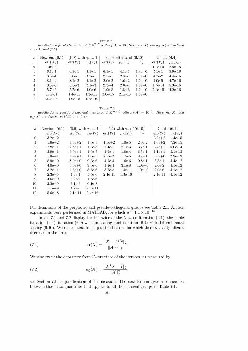
Table 7.1Results for a perplectic matrix A ∈ R7×7 with κ2(A) = 10. Here, err(X) and µ

G(X) are defined

in (7.1) and (7.2).

k Newton, (6.1) (6.9) with γk ≡ 1 (6.9) with γk of (6.10) Cubic, (6.4)err(Xk) err(Yk) µG(Yk) err(Yk) µG(Yk) γk err(Yk) µG(Yk)

0 1.0e+0 1.0e+0 2.5e-151 6.1e-1 6.1e-1 4.1e-1 6.1e-1 4.1e-1 1.4e+0 5.1e-1 8.9e-162 3.6e-1 3.6e-1 3.7e-1 2.5e-1 2.3e-1 1.1e+0 4.7e-2 4.4e-163 8.1e-2 8.1e-2 5.1e-2 2.0e-2 1.6e-2 1.0e+0 4.0e-5 4.7e-164 3.5e-3 3.5e-3 2.1e-3 2.3e-4 2.0e-4 1.0e+0 1.7e-14 5.3e-165 5.7e-6 5.7e-6 4.0e-6 1.9e-8 1.5e-8 1.0e+0 2.1e-15 4.2e-166 1.4e-11 1.4e-11 1.3e-11 2.0e-15 2.1e-16 1.0e+07 2.2e-15 1.9e-15 1.2e-16

Table 7.2Results for a pseudo-orthogonal matrix A ∈ R10×10 with κ2(A) = 1010. Here, err(X) and

µG(X) are defined in (7.1) and (7.2).

k Newton, (6.1) (6.9) with γk ≡ 1 (6.9) with γk of (6.10) Cubic, (6.4)err(Xk) err(Yk) µG(Yk) err(Yk) µG(Yk) γk err(Yk) µG(Yk)

0 3.2e+2 3.2e+2 1.4e-151 1.6e+2 1.6e+2 1.0e-5 1.6e+2 1.0e-5 2.0e-2 1.0e+2 7.2e-152 7.8e+1 7.8e+1 1.0e-5 7.4e-1 2.1e-3 3.7e-1 3.4e+1 6.0e-143 3.9e+1 3.9e+1 1.0e-5 1.9e-1 1.8e-4 6.5e-1 1.1e+1 5.1e-134 1.9e+1 1.9e+1 1.0e-5 6.0e-2 1.7e-5 8.7e-1 3.0e+0 2.9e-125 8.9e+0 8.9e+0 9.9e-6 4.9e-3 1.6e-6 9.8e-1 5.5e-1 4.4e-126 4.0e+0 4.0e+0 9.6e-6 1.2e-4 3.1e-8 1.0e+0 2.0e-2 4.1e-127 3.2e+1 1.6e+0 8.5e-6 3.6e-8 1.4e-11 1.0e+0 2.0e-6 4.1e-128 2.3e+5 4.9e-1 5.5e-6 2.1e-11 1.3e-16 2.1e-11 4.1e-129 4.6e+9 8.2e-2 1.5e-6

10 2.3e+9 3.1e-3 6.1e-811 1.1e+9 4.7e-6 9.5e-1112 5.6e+8 2.1e-11 2.4e-16

For definitions of the perplectic and pseudo-orthogonal groups see Table 2.1. All ourexperiments were performed in MATLAB, for which u ≈ 1.1 × 10−16.

Tables 7.1 and 7.2 display the behavior of the Newton iteration (6.1), the cubiciteration (6.4), iteration (6.9) without scaling, and iteration (6.9) with determinantalscaling (6.10). We report iterations up to the last one for which there was a significantdecrease in the error

err(X) =‖X − A1/2‖2

‖A1/2‖2.(7.1)

We also track the departure from G-structure of the iterates, as measured by

µG(X) =‖X⋆X − I‖2

‖X‖22

;(7.2)

see Section 7.1 for justification of this measure. The next lemma gives a connectionbetween these two quantities that applies to all the classical groups in Table 2.1.

25

Lemma 7.1. Let A ∈ G, where G is the automorphism group of any scalar product

for which M is unitary. Then for X ∈ Kn×n close to A1/2 ∈ G,

µG(X) ≤ 2err(X) + O(err(X)2).(7.3)

Proof. Let A ∈ G and X = A1/2 + E. Then

X⋆X − I = (A1/2)⋆(A1/2 + E) + E⋆A1/2 + E⋆E − I

= A−1/2E + E⋆A1/2 + E⋆E.

Taking 2-norms and using (2.1) and (2.2) gives

‖X⋆X − I‖2 ≤ ‖E‖2(‖A−1/2‖2 + ‖A1/2‖2) + ‖E‖22

= 2‖E‖2 ‖A1/2‖2 + ‖E‖22.

The result follows on multiplying throughout by ‖X‖−22 and noting that ‖X‖−2

2 =‖A1/2‖−2

2 + O(‖E‖2).

The analysis in Section 6 shows that for A ∈ G the Newton iteration (6.1) anditeration (6.9) without scaling generate precisely the same sequence, and this explainsthe equality of the errors in the first two columns of Tables 7.1 and 7.2 for 1 ≤ k ≤ 6.But for k > 6 the computed Newton sequence diverges for the pseudo-orthogonalmatrix, manifesting the well known instability of the iteration (even for symmetricpositive definite matrices). Table 7.2 shows that scaling brings a clear reduction in thenumber of iterations for the pseudo-orthogonal matrix and makes the scaled iteration(6.9) more efficient than the cubic iteration in this example.

The analysis of Section 5 shows that the cubic structure-preserving iteration isstable, and for the classical groups it provides an estimate (1 + ‖A1/2‖2

2)u of therelative limiting accuracy. This fits well with the observed errors in Table 7.2, since inthis example ‖A1/2‖2

2 = ‖A‖2 = 105 (which follows from the fact that A is symmetricpositive definite).

The analysis mentioned at the end of Section 5 shows that the unscaled iteration(6.7) is also stable if the adjoint is involutory, and the same estimate of the relativelimiting accuracy as for the cubic iteration is obtained for the classical groups. Thesefindings again match the numerical results very well.

The original Newton iteration (6.1) has a Frechet derivative map whose powers

are bounded if the eigenvalues λi of A satisfy 12 |1 − λ

1/2i λ

−1/2j | < 1 for all i and j

[11]. This condition is satisfied for our first test matrix, but not for the second. Theterm on the left of this inequality also arises in Lemma 5.4 with B = A1/2. Hence ourtheory predicts that the variant of (6.4) that corresponds to (5.4), in which (6.4b) isreplaced by Zk+1 = 1

3Zk[I + 8(I + 3ZkYk)−1], will be unstable for the second matrix.Indeed it is, with minimum error 7.5e-3 occurring at k = 7, after which the errorsincrease; it is stable for the first matrix.

Turning to the preservation of structure, the values for µG(Yk) in the tables con-

firm that the cubic iteration is structure preserving. But Table 7.2 also reveals thatfor the pseudo-orthogonal matrix, iteration (6.9), with or without scaling, is numer-ically better at preserving group structure at convergence than the cubic structure-preserving iteration, by a factor 104. The same behavior has been observed in otherexamples. Partial explanation is provided by the following lemma.

26

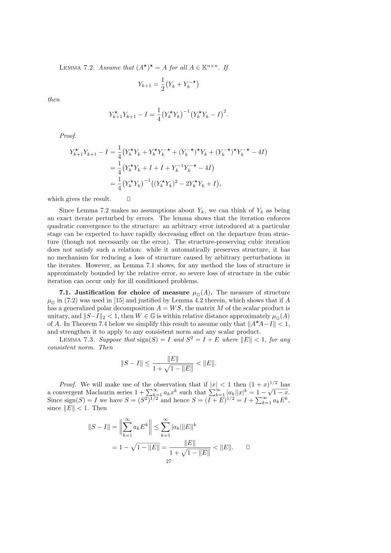
Lemma 7.2. Assume that (A⋆)⋆ = A for all A ∈ Kn×n. If

Yk+1 =1

2

(Yk + Y −⋆

k

)

then

Y ⋆k+1Yk+1 − I =

1

4

(Y ⋆

k Yk

)−1(

Y ⋆k Yk − I

)2.

Proof.

Y ⋆k+1Yk+1 − I =

1

4

(Y ⋆

k Yk + Y ⋆k Y −⋆

k + (Y −⋆k )⋆Yk + (Y −⋆

k )⋆Y −⋆k − 4I

)

=1

4

(Y ⋆

k Yk + I + I + Y −1k Y −⋆

k − 4I)

=1

4

(Y ⋆

k Yk

)−1(

(Y ⋆k Yk)2 − 2Y ⋆

k Yk + I),

which gives the result.

Since Lemma 7.2 makes no assumptions about Yk, we can think of Yk as beingan exact iterate perturbed by errors. The lemma shows that the iteration enforcesquadratic convergence to the structure: an arbitrary error introduced at a particularstage can be expected to have rapidly decreasing effect on the departure from struc-ture (though not necessarily on the error). The structure-preserving cubic iterationdoes not satisfy such a relation: while it automatically preserves structure, it hasno mechanism for reducing a loss of structure caused by arbitrary perturbations inthe iterates. However, as Lemma 7.1 shows, for any method the loss of structure isapproximately bounded by the relative error, so severe loss of structure in the cubiciteration can occur only for ill conditioned problems.

7.1. Justification for choice of measure µG(A). The measure of structure

µG

in (7.2) was used in [15] and justified by Lemma 4.2 therein, which shows that if Ahas a generalized polar decomposition A = WS, the matrix M of the scalar product isunitary, and ‖S−I‖2 < 1, then W ∈ G is within relative distance approximately µ

G(A)

of A. In Theorem 7.4 below we simplify this result to assume only that ‖A⋆A−I‖ < 1,and strengthen it to apply to any consistent norm and any scalar product.

Lemma 7.3. Suppose that sign(S) = I and S2 = I + E where ‖E‖ < 1, for any

consistent norm. Then

‖S − I‖ ≤ ‖E‖1 +

√1 − ‖E‖

< ‖E‖.

Proof. We will make use of the observation that if |x| < 1 then (1 + x)1/2 hasa convergent Maclaurin series 1 +

∑∞

k=1 akxk such that∑

∞

k=1 |ak||x|k = 1 −√

1 − x.Since sign(S) = I we have S = (S2)1/2 and hence S = (I + E)1/2 = I +

∑∞

k=1 akEk,since ‖E‖ < 1. Then

‖S − I‖ =

∥∥∥∥∞∑

k=1

akEk

∥∥∥∥ ≤∞∑

k=1

|ak|‖E‖k

= 1 −√

1 − ‖E‖ =‖E‖

1 +√

1 − ‖E‖< ‖E‖.

27

The following theorem generalizes [12, Lem. 5.1], [14, Lem. 5.3] and [15, Lem. 4.2].Theorem 7.4. Let G be the automorphism group of a scalar product. Suppose

that A ∈ Kn×n satisfies (A⋆)⋆ = A and ‖A⋆A − I‖ < 1. Then A has a generalized

polar decomposition A = WS and, for any consistent norm, the factors W and Ssatisfy

‖A⋆A − I‖‖A‖(‖A⋆‖ + ‖W⋆‖) ≤ ‖A − W‖

‖A‖ ≤ ‖A⋆A − I‖‖A‖2

‖A‖ ‖W‖,(7.4)

‖A⋆A − I‖‖S‖ + ‖I‖ ≤ ‖S − I‖ ≤ ‖A⋆A − I‖.(7.5)

The inequalities (7.4) can be rewritten as

µG(A)‖A‖

‖A⋆‖ + ‖W⋆‖ ≤ ‖A − W‖‖A‖ ≤ µG(A) ‖A‖ ‖W‖.

Proof. The condition ‖A⋆A − I‖ < 1 implies that the spectral radius of A⋆A − Iis less than 1, and hence that A⋆A has no eigenvalues on R

−. Since (A⋆)⋆ = A,Theorem 4.1 implies that A has a (unique) generalized polar decomposition A = WS.Using W⋆ = W−1 and S⋆ = S we have

(A + W )⋆(A − W ) = A⋆A − A⋆W + W⋆A − W⋆W

= A⋆A − S⋆W⋆W + W⋆WS − I = A⋆A − I.

The lower bound in (7.4) follows on taking norms and using ‖(A + W )⋆‖ = ‖A⋆ +W⋆‖ ≤ ‖A⋆‖ + ‖W⋆‖.

The upper bound in (7.5) follows from Lemma 7.3, since

A⋆A − I = S⋆W⋆WS − I = S2 − I.(7.6)

The upper bound in (7.4) then follows by taking norms in A−W = WS−W = W (S−I). Finally, the lower bound in (7.5) follows by writing (7.6) as A⋆A−I = (S−I)(S+I)and taking norms.

Note that the term ‖A⋆‖ in the denominator of (7.4) can be replaced by κ(M)‖AT ‖or κ(M)‖A∗‖ for bilinear forms and sesquilinear forms, respectively, and for a uni-tarily invariant norm both expressions are just ‖A‖ for all the groups in Table 2.1;likewise for ‖W⋆‖.

7.2. Conclusions on choice of method for A1/2 when A ∈ G. Our overallconclusion is that the rewritten form (6.9) of Newton’s iteration, with the scaling(6.10) or perhaps some alternative, is the best iteration method for computing thesquare root of a matrix A in an automorphism group. This iteration

• Overcomes the instability in the standard Newton iteration (6.1) and is lesscostly per iteration than (6.1) for the classical groups.

• Is generally more efficient than the cubic structure-preserving iteration (6.4):it costs significantly less per iteration than (6.4), and (6.4) typically requiresapproximately the same number of iterations.

• When iterated to convergence to machine precision, is likely to produce acomputed result lying closer to the group than the cubic iteration (6.4) whenA is ill conditioned.

28

• For the classical groups has half the cost per iteration of the mathematicallyequivalent Denman–Beavers iteration recommended in [13]. In fact, anotherway to derive (6.7) is to exploit the structure in the Denman–Beavers iterationthat results when A ∈ G.

If a structure-preserving iteration is required then an iteration from the family (6.2)can be recommended, such as the cubically convergent iteration (6.4). These itera-tions have the advantage that even if they are terminated well before convergence tomachine precision, the result will lie in the group to approximately machine precision,though some loss of structure (no worse than that described by (7.3)) may occur forill conditioned problems.

REFERENCES

[1] Dario A. Bini, Nicholas J. Higham, and Beatrice Meini, Computing the matrix pth root,numerical analysis report, Manchester Centre for Computational Mathematics, Manch-ester, England, 2004. In preparation.

[2] Yuri Bolshakov, Cornelis V. M. van der Mee, Andre C. M. Ran, Boris Reichstein, andLeiba Rodman, Extension of isometries in finite-dimensional indefinite scalar product

spaces and polar decompositions, SIAM J. Matrix Anal. Appl., 18 (1997), pp. 752–774.[3] Yuri Bolshakov, Cornelis V. M. van der Mee, Andre C. M. Ran, Boris Reichstein,

and Leiba Rodman, Polar decompositions in finite dimensional indefinite scalar product

spaces: General theory, Linear Algebra Appl., 261 (1997), pp. 91–141.[4] Ralph Byers, Solving the algebraic Riccati equation with the matrix sign function, Linear

Algebra Appl., 85 (1987), pp. 267–279.[5] Joao R. Cardoso, Charles S. Kenney, and F. Silva Leite, Computing the square root and

logarithm of a real P -orthogonal matrix, Appl. Numer. Math., 46 (2003), pp. 173–196.[6] Henri Cartan, Differential Calculus, Hermann, Paris, 1971.[7] Sheung Hun Cheng, Nicholas J. Higham, Charles S. Kenney, and Alan J. Laub, Ap-

proximating the logarithm of a matrix to specified accuracy, SIAM J. Matrix Anal. Appl.,22 (2001), pp. 1112–1125.

[8] Israel Gohberg, Peter Lancaster, and Leiba Rodman, Matrices and Indefinite Scalar

Products, Birkhauser, Basel, Switzerland, 1983.[9] Robert E. Greene and Steven G. Krantz, Function Theory of One Complex Variable,

Wiley, New York, 1997.[10] Nicholas J. Higham, Computing the polar decomposition—with applications, SIAM J. Sci.

Statist. Comput., 7 (1986), pp. 1160–1174.[11] , Newton’s method for the matrix square root, Math. Comp., 46 (1986), pp. 537–549.[12] , The matrix sign decomposition and its relation to the polar decomposition, Linear

Algebra Appl., 212/213 (1994), pp. 3–20.[13] , Stable iterations for the matrix square root, Numerical Algorithms, 15 (1997), pp. 227–

242.[14] , J-orthogonal matrices: Properties and generation, SIAM Rev., 45 (2003), pp. 504–519.[15] Nicholas J. Higham, D. Steven Mackey, Niloufer Mackey, and Francoise Tisseur,

Computing the polar decomposition and the matrix sign decomposition in matrix groups,Numerical Analysis Report No. 426, Manchester Centre for Computational Mathematics,Manchester, England, Apr. 2003. Revised November 2003. To appear in SIAM J. MatrixAnal. Appl.

[16] Roger A. Horn and Charles R. Johnson, Topics in Matrix Analysis, Cambridge UniversityPress, 1991.

[17] Khakim D. Ikramov, Hamiltonian square roots of skew-Hamiltonian matrices revisited, LinearAlgebra Appl., 325 (2001), pp. 101–107.

[18] David P. Jagger, MATLAB toolbox for classical matrix groups, M.Sc. Thesis, University ofManchester, Manchester, England, Sept. 2003.

[19] Irving Kaplansky, Algebraic polar decomposition, SIAM J. Matrix Anal. Appl., 11 (1990),pp. 213–217.

[20] Charles S. Kenney and Alan J. Laub, Rational iterative methods for the matrix sign func-

tion, SIAM J. Matrix Anal. Appl., 12 (1991), pp. 273–291.[21] , On scaling Newton’s method for polar decomposition and the matrix sign function,

SIAM J. Matrix Anal. Appl., 13 (1992), pp. 688–706.

29

[22] , The matrix sign function, IEEE Trans. Automat. Control, 40 (1995), pp. 1330–1348.[23] Pentti Laasonen, On the iterative solution of the matrix equation AX2 − I = 0, M.T.A.C.,

12 (1958), pp. 109–116.[24] Peter Lancaster and Miron Tismenetsky, The Theory of Matrices, Academic Press, Lon-

don, second ed., 1985.[25] D. Steven Mackey, Niloufer Mackey, and Francoise Tisseur, Structured tools for struc-

tured matrices, The Electronic Journal of Linear Algebra, 10 (2003), pp. 106–145.[26] , Structured factorizations in scalar product spaces, Numerical Analysis Report No. 432,

Manchester Centre for Computational Mathematics, Manchester, England, 2004. In prepa-ration.

[27] Reinhold Remmert, Theory of Complex Functions, Springer-Verlag, Berlin, 1991.[28] J. D. Roberts, Linear model reduction and solution of the algebraic Riccati equation by use

of the sign function, Internat. J. Control, 32 (1980), pp. 677–687. First issued as reportCUED/B-Control/TR13, Department of Engineering, University of Cambridge, 1971.

[29] Jacob T. Schwartz, Nonlinear Functional Analysis, Gordon and Breach, New York, 1969.

30