matrix factorization and collaborative filteringacsweb.ucsd.edu/~dklim/mf_presentation.pdfmatrix...

Matrix Factorization and Collaborative Filtering

Daryl Lim

University of California, San Diego

February 7, 2013

Presentation Outline

1 Overview

2 PCAIntuitionMatrix Factorization ViewpointPCA vs SVDConsiderations and LimitationsWorked Example

3 Non-negative Matrix FactorizationLearning

4 Collaborative FilteringNeighborhood-based approachMatrix Factorization ApproachLimitationsExtensions

Matrix Factorization: Overview

Given a matrix X ∈ Rm×n,m ≤ n, we want to find matricesU, V such that X ≈ UV = X

In this talk, we consider the scenario when X is low-rank

X U

V

^

Why are low-rank approximations important?

Intuitively, if matrix is low rank, then the observations can beexplained by linear combinations of few underlying factorsWant to know which factors control the observations

Collaborative Filtering: Overview

Given a list of users and items, and user-item interactions,predict user behavior

Key idea: Use only user-item interactions to predict behavior

iTunes Genius

Contrast with content-based filtering, which builds a modelfor each item

e.g. Pandora hires musicologists to characterize songs, builtthe Music Genome

Matrix Factorization

This Talk

Matrix factorization for dimensionality reduction (PrincipalComponents Analysis or PCA)

Non-negative Matrix Factorization, a related factorizationmethod

Matrix factorization methods for collaborative filteringapplications

Principal Components Analysis

What can we do with PCA?

Dimensionality reduction: Can we represent each data pointwith fewer features, without losing much?

Yes, if there is redundancy in the data!

Data understanding: Which variables contribute to the largestvariations in the data?

Look at the components of each principal component

Principal Components Analysis

What does PCA do?

PCA finds a set of vectors called principal components thatdescribe the data in an alternative way.

The first principal component (PC) is the vector thatmaximizes the variance of the projected data.

The kth PC is the vector orthogonal to all k − 1 PCs thatmaximizes the variance of the projected data

Equivalently, we can think of PCA as learning a rotation ofthe canonical axes to align with these principal components,while the data cloud is fixed

Nice effect of this transformation is that the covariance matrixof the transformed data is diagonal

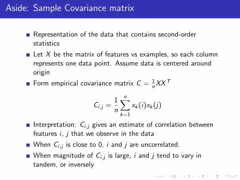
Aside: Sample Covariance matrix

Representation of the data that contains second-orderstatistics

Let X be the matrix of features vs examples, so each columnrepresents one data point. Assume data is centered aroundorigin

Form empirical covariance matrix C = 1nXXT

Ci ,j =1

n

n∑k=1

xk(i)xk(j)

Interpretation: Ci ,j gives an estimate of correlation betweenfeatures i , j that we observe in the data

When Ci ,j is close to 0, i and j are uncorrelated.

When magnitude of Ci ,j is large, i and j tend to vary intandem, or inversely

Principal Components Analysis: Intuition

Diagonal entries of C denote variance of each attribute.

Assumption: Large values of variance are more interesting, andwe want to preserve them.

Off-diagonal entries of C denote covariances of each attribute.

Assumption: Large magnitudes on Cij , i 6= j denoteredundancy between i and je.g. mean weekly rainfall, mean daily rainfall

Principal Components Analysis: Intuition

Why is a diagonal covariance matrix desirable?

Diagonal covariance matrix allows us to see exactly how muchvariance each feature contains

Diagonal covariance matrix means features are decorrelated

Gives us a principled way to perform dimensionality reductionby removing features of lowest variance!

Principal Components Analysis Formulation

Present a formulation which leads to solution in a simple way(though it is not from first principles)

PCA problem: Find an orthonormal matrix W such thatY = WX has a diagonal covariance matrix 1

nYY T , where thevariances are ordered from largest to smallest

Then, rows of W give us the principal components

Principal Components Analysis Formulation

Fact: Any symmetric matrix M can be represented asM = QΛQT , where Q is orthonormal and Λ is diagonal.

Columns of Q are the eigenvectors of X and the diagonalentries of Λ are associated eigenvalues

Since C = XXT is symmetric, we can express 1nYY T as

1

nYY T =

1

n(WX )(WX )T

=1

nWXXTW T

= WCW T

= WQΛQW T

Setting W = QT gives 1nYY T = QTQΛQTQ = I ΛI = Λ

which is diagonal as desired.

PCA: Matrix Factorization Viewpoint

So far, the PCA solution is Y = QTX , whereQ = [q1, q2 · · · qn] is a matrix of principal components, and Λis a diagonal matrix of corresponding eigenvalues ordered fromlargest to smallest

Let’s consider a single data point y = QT x

Then the ith coordinate y(i) = qTi x is the orthogonal

projection of x onto the ith principal component.

To perform dimensionality reduction, discard the bottomfeatures of y , as they correspond to directions of smallestvariance


If we retain all values of Y , We can recover X perfectly asX = (QT )−1Y = QY (property of orthonormal matrix Q)

However, what if we removed the k features of Ycorresponding to smallest variance

Then, we can only recover X = QY where Y = Y with the kfeatures with smallest variance set to 0


0~~

Y~Q~

Q YX

Q~Y~

Q~'

X

It turns out, approximation of X in this way by the top kcomponents of Y minimizes ‖X − X‖2F over all rank-k

matrices X

Singular Value Decomposition

Any matrix X ∈ Rm×n can be represented as

X = USV T

where U ∈ Rm×m and V ∈ Rn×n are orthonormal andS ∈ Rm×n is nonzero only on the diagonal

We can obtain the PCA solution from SVD, without having toform the covariance matrix 1

nXXT explicitly

Popular languages such as R, Matlab, Python have SVDroutines.

Link between PCA and SVD

Substitute X = USV T in the equation for the covariancematrix.

Then, we obtain

XXT = USV TVSTU = U(SST )U

where (SST ) is diagonal

We can see immediately that U(SST )U has the samestructure as QΛQT

Therefore, the U matrix in the SVD is exactly the Q matrixwe are trying to obtain in the PCA problem (up to signchanges on eigenvectors)

PCA: Considerations

How many components to keep?

Typically, retain enough dimensions to explain large proportionof the variance (common heuristic is 95%)

The total variance is exactly the sum of the eigenvalues of1nXXT

Keep adding successive PCs until the cumulative sum ofrespective eigenvalues hits the desired proportion

PCA: Considerations

Is it necessary to preprocess or scale the data?

Should always make data zero mean, otherwise the PCs foundwill not be what is expected

PC1

PC1

PCA: Considerations

Is it necessary to preprocess or scale the data?

Scaling features arbitrarily (for example converting height infeet to inches) skews the PCs considerably

In general, if features are of different orders of magnitude, ordifferent units, usually scale each feature to zero mean andunit standard deviation (z-scoring)

If features are on same scale (e.g. exam scores for differentsubjects) then no scaling is needed

Much discussion about the issue

PCA: Limitations

Depending on task, the strongly predictive information may liein directions of small variance, which gets removed by PCA

e.g. predicting size of clothes purchased, using income, taxes,height

Solution: Use supervised dimensionality reduction techniques(e.g. distance metric learning algorithms) which retainkeeping features useful for a (classification/regression) task

Tradeoff: computational and implementational complexity.

PCA: Limitations

−5 0 5

−6

−4

−2

0

2

4

6

−5 0 5

−6

−4

−2

0

2

4

6

Blue and red dots are data points from different classes

Without class information, 1-dimensional PCA projectionshown on right

Classes are separable with both features but not afterprojection

PCA: Limitations

PCA finds linear projections

If data lies near or on a non-linear manifold (e.g. swiss roll),linear projection may not preserve distances along manifoldSolution: Use manifold learning techniques such as LocallyLinear Embedding (LLE) 1, which may be able to learn betterprojections for the data

−10 0 10 200

20

−15

−10

−5

0

5

10

15

Full Data

−25 −20 −15 −10 −5 0 5−15

−10

−5

0

5

10

15

PCA

−2 −1 0 1 2−1

−1

−1

−1

−1

−1

−1

−1

−1

LLE

1Sam T. Roweis and Lawrence K. Saul. Nonlinear dimensionality reductionby locally linear embedding.SCIENCE, 290:2323–2326, 2000

Principal Components Analysis Worked Example

For a concrete example, let’s use the 2004 Cars dataset fromthe Journal of Statistics Education

Dataset comprises different models of cars and their features

Each car described by 11 features

Matlab code only takes 4 lines (the svd function already sortsPC by eigenvalue

load cars

X = zscore(X’)’;

[PC Sigma V] = svd(X); %PC = principal components

Y = PC’*X;


1 Retail Price2 Dealer Cost3 Engine Size4 #Cylinders5 Horsepower6 City MPG

7 Highway MPG8 Weight9 Wheelbase10 Length11 Width

−6 −4 −2 0 2 4 6 8−4

−3

−2

−1

0

1

2

3

4

Projection of cars onto 1st PC

Regular cars

Sports Cars

SUVs

Wagons/Minivans

1 2 3 4 5 6 7 8 9 10 11−0.4

−0.3

−0.2

−0.1

0

0.1

0.2

0.3

0.4First principal component




−8 −6 −4 −2 0 2

−3

−2

−1

0

1

2

3

Projection of cars onto 2nd PC

Regular cars

Sports Cars

SUVs

Wagons/Minivans

1 2 3 4 5 6 7 8 9 10 11−0.5

0

0.5Second principal component




−8 −6 −4 −2 0 2 4 6 8

−8

−6

−4

−2

0

2

Projection onto 1st PC

Pro

jectio

n o

nto

2n

d P

C

Projection of cars onto 2 PCs

Regular cars

Sports Cars

SUVs

Wagons/Minivans1 2 3 4 5 6 7 8 9 10 11

0.65

0.7

0.75

0.8

0.85

0.9

0.95

1Cumulative proportion of variance explained

Non-negative Matrix Factorization

Another popular matrix factorization method

We want to minimize the norm ‖X −WY ‖2F , whereW ∈ Rm×k , Y ∈ Rk×n

So far, exactly the same as PCA

As the name suggests, all matrices X , W and Y must containonly non-negative elements.


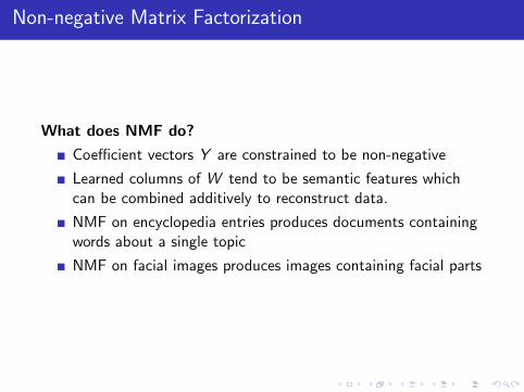
What does NMF do?

Coefficient vectors Y are constrained to be non-negative

Learned columns of W tend to be semantic features whichcan be combined additively to reconstruct data.

NMF on encyclopedia entries produces documents containingwords about a single topic

NMF on facial images produces images containing facial parts


2

2D. D. Lee and H. S. Seung. Learning the parts of objects by non-negativematrix factorization.Nature, 401(6755):788–791, October 1999


Learning NMF

NMF can only find a local minimum of the error as theproblem is nonconvex

However, it can be minimized by a simple multiplicative form

Yij ← Yij(W TX )ij

(W TWY )ij, Wij ←Wij

(XY T )ij(XYY T )ij

and iterating until convergence

Can be implemented in fewer than 10 lines

Collaborative Filtering Algorithms

Given a list of users and items, and user-item interactions,predict user behavior

What do we want to predict?

This talk: Predict unobserved ratings of item j for user i

Recent work on predicting rankings of unrated/unpurchaseditems for each user


Problem: Predict score/affinity of item j for user i .

User-based approachFind a set of users Si who rated item j , that are most similarto ui

compute predicted Vij score as a function of ratings of item jgiven by Si (usually weighted linear combination)

Item-based approachFind a set of most similar items Sj to the item j which wererated by ui

compute predicted Vij score as a function of ui ’s ratings for Sj


Users

Items

1 2 ?

5 4

1 3 2

5

2 1

1

2

3

14Users

Items

1 2 ?

5 4

1 3 2

5

2 1

1

2

3

14

Users

Items

1 2 ?

5 4

1 3 2

5

2 1

1

2

3

14

How to compute similarity between users/items?

Cosine similarity

s(x , y) =xT y

‖x‖‖y‖and its variants (e.g. adding weights/biases)

Matrix Factorization for Collaborative Filtering - Model

Let’s consider items for sale on an e-commerce site

Represent user i as a vector of preferences for a few factors pi

e.g. ”ease of use”, ”value for money”, ”aesthetic appeal”pi = [0.7 0.1 0.6] = user i likes items which are easy to useand look nice, and doesn’t mind paying for it


Represent item j as a vector qj where each element expresseshow much the item exhibits that factor

Rating of an item is estimated by pTi qj

Intuition: if there is high correlation between thecharacteristics item exhibits that a user likes, he should givethe item a high rating


Problem: How to describe items with factors?

Solution: Learn latent representation using the SVD

Caveat: We don’t learn semantic interpretations of thefactors, just the numerical representations of the users/items

However, for each factor, we can see which items havehigh/low scores, and assign human interpretations to thatfactor

This is what Netflix does for movies, in their recommendationsystem (example factors: ”Strong Female Lead”, ”CerebralSuspense”)

Matrix Factorization for Collaborative Filtering

Assume we are given data X ∈ Rm×n is a large matrix,comprising ratings of n movies by m users.

Using our earlier model (Xi j = pTi qj), we can approximate X

by X = PQ, and rank X = k , the number of factors

X

q1 n2qp12p

pm

q

^ =

k

For a given number of factors k, SVD gives us the optimalfactorization which globally minimizes ‖X − X‖2F the meansquared prediction error over all user-item pairs!


Limitations of SVD method for Collaborative Filtering

SVD can only be applied if we know all the user-item ratings

e.g. Netflix Prize - only 1% of ratings given

SVD is only able to minimize the (squared) Frobenius normloss - may not be appropriate

SVD is very slow for a large, dense user-item matrix


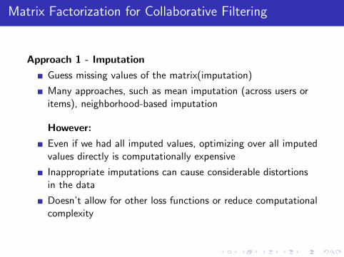
Approach 1 - Imputation

Guess missing values of the matrix(imputation)

Many approaches, such as mean imputation (across users oritems), neighborhood-based imputation

However:

Even if we had all imputed values, optimizing over all imputedvalues directly is computationally expensive

Inappropriate imputations can cause considerable distortionsin the data

Doesn’t allow for other loss functions or reduce computationalcomplexity


Approach 2 - Beyond SVD

Minimize loss only over observed values, i.e.∑

i ,j(Xij − pTi qj)

where (i , j) is an observed user-item rating pair

Reduce computational complexityHave to regularize P, Q to prevent overfitting

Instead of using SVD, use methods like alternating leastsquares or stochastic gradient descent to update parameters

Allows more flexible model, and incorporating different lossfunctions (e.g. adding biases/temporal dynamics)Drawback: Lots of parameters/hyperparameters to tune!

Simon Funk ”Try This at Home”

Performance on Netflix Dataset

3

3Yehuda Koren, Robert Bell, and Chris Volinsky. Matrix factorizationtechniques for recommender systems.Computer, 42(8):30–37, August 2009

Other approaches to collaborative filtering

Collaborative Ranking

Instead of rating prediction, predict a ranked list of items usermight find usefulPromising idea which can achieve state-of-the-art performance

Nonnegative Matrix Factorization for Collaborative Filtering

NMF has also been used successfully to model movie ratingsUses Expectation-Maximization approach to deal with missingvalues

Other approaches to collaborative filtering

Hybrid recommendation systems

Combine content-based and collaborative filtering into a singlemodelAllows to integrate prior domain knowledge (e.g. informationabout items) into recommendationAlleviates the cold-start problem for items with very few ratings

Conclusion

Matrix factorizations are an important class of tools today

Use spans dimensionality reduction, data understanding,prediction

Simple methods like PCA can produce interesting insights ofthe data

Questions

Thank you!

Questions?

matrix factorization and collaborative filteringacsweb.ucsd.edu/~dklim/mf_presentation.pdfmatrix...

Documents