Kernelized Matrix Factorization for Collaborative Filtering

Xinyue Liu∗ Charu Aggarwal † Yu-Feng Li ‡ Xiangnan Kong∗ Xinyuan Sun∗

Saket Sathe §

Abstract

Matrix factorization (MF) methods have shown greatpromise in collaborative filtering (CF). ConventionalMF methods usually assume that the correlated data isdistributed on a linear hyperplane, which is not alwaysthe case. Kernel methods are used widely in SVMs toclassify linearly non-separable data, as well as in PCAto discover the non-linear embeddings of data. In thispaper, we present a novel method to kernelize matrixfactorization for collaborative filtering, which is equiva-lent to performing the low-rank matrix factorization ina possibly much higher dimensional space that is im-plicitly defined by the kernel function. Inspired by thesuccess of multiple kernel learning (MKL) methods, wealso explore the approach of learning multiple kernelsfrom the rating matrix to further improve the accuracyof prediction. Since the right choice of kernel is usuallyunknown, our proposed multiple kernel matrix factor-ization method helps to select effective kernel functionsfrom the candidates. Through extensive experiments onreal-world datasets, we show that our proposed methodcaptures the nonlinear correlations among data, whichresults in improved prediction accuracy compared to thestate-of-art CF models.

1 Introduction

With the sheer growth of accessible online data, it be-comes challenging as well as indispensable to developtechnologies that helping people efficiently sift throughthe huge amount of information. Collaborative filter-ing is one of these technologies which has drawn muchattention in recent years. It mainly serves as a recom-mender system to automatically generate item recom-mendations based on past user-item feedbacks. Com-pared to other technologies in recommender systems,collaborative filtering does not need any content infor-mation about the items or users, it works by purely

∗Department of Computer Science, Worcester PolytechnicInstitute†IBM T. J. Watson Research Center‡Nanjing University§IBM Research Australia

5 3 ? ?? 4 2 43 5 ? 2? ? ? 5? 1 ? ?

U

V

=

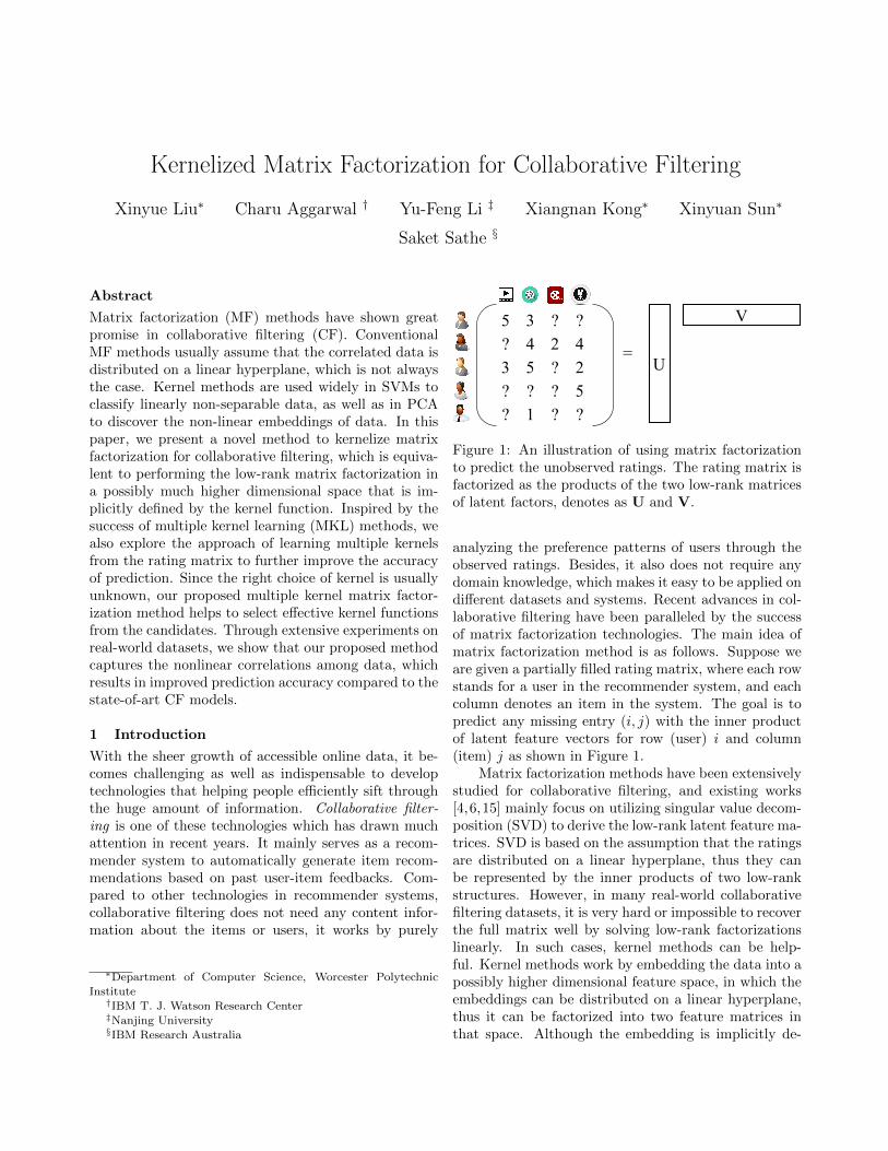
Figure 1: An illustration of using matrix factorizationto predict the unobserved ratings. The rating matrix isfactorized as the products of the two low-rank matricesof latent factors, denotes as U and V.

analyzing the preference patterns of users through theobserved ratings. Besides, it also does not require anydomain knowledge, which makes it easy to be applied ondifferent datasets and systems. Recent advances in col-laborative filtering have been paralleled by the successof matrix factorization technologies. The main idea ofmatrix factorization method is as follows. Suppose weare given a partially filled rating matrix, where each rowstands for a user in the recommender system, and eachcolumn denotes an item in the system. The goal is topredict any missing entry (i, j) with the inner productof latent feature vectors for row (user) i and column(item) j as shown in Figure 1.

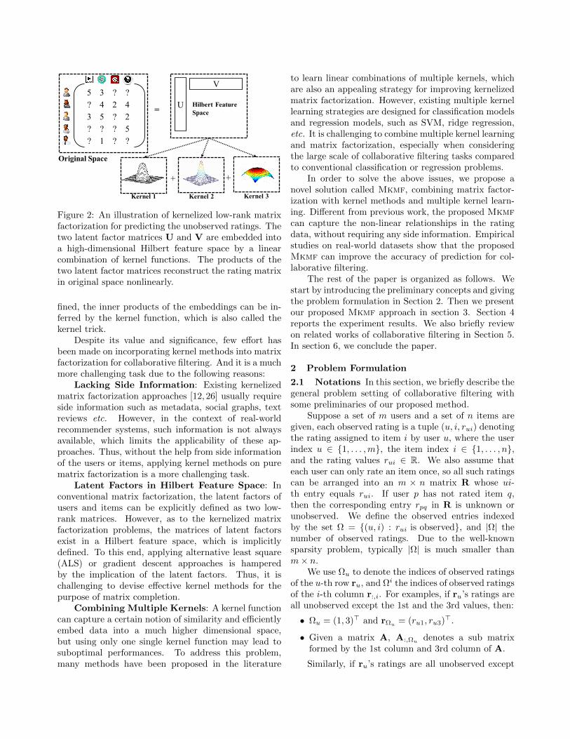
Matrix factorization methods have been extensivelystudied for collaborative filtering, and existing works[4,6,15] mainly focus on utilizing singular value decom-position (SVD) to derive the low-rank latent feature ma-trices. SVD is based on the assumption that the ratingsare distributed on a linear hyperplane, thus they canbe represented by the inner products of two low-rankstructures. However, in many real-world collaborativefiltering datasets, it is very hard or impossible to recoverthe full matrix well by solving low-rank factorizationslinearly. In such cases, kernel methods can be help-ful. Kernel methods work by embedding the data into apossibly higher dimensional feature space, in which theembeddings can be distributed on a linear hyperplane,thus it can be factorized into two feature matrices inthat space. Although the embedding is implicitly de-

5 3 ? ?? 4 2 43 5 ? 2? ? ? 5? 1 ? ?

U= Hilbert Feature Space

V

Kernel 1 Kernel 2 Kernel 3

Original Space

+ +

Figure 2: An illustration of kernelized low-rank matrixfactorization for predicting the unobserved ratings. Thetwo latent factor matrices U and V are embedded intoa high-dimensional Hilbert feature space by a linearcombination of kernel functions. The products of thetwo latent factor matrices reconstruct the rating matrixin original space nonlinearly.

fined, the inner products of the embeddings can be in-ferred by the kernel function, which is also called thekernel trick.

Despite its value and significance, few effort hasbeen made on incorporating kernel methods into matrixfactorization for collaborative filtering. And it is a muchmore challenging task due to the following reasons:

Lacking Side Information: Existing kernelizedmatrix factorization approaches [12, 26] usually requireside information such as metadata, social graphs, textreviews etc. However, in the context of real-worldrecommender systems, such information is not alwaysavailable, which limits the applicability of these ap-proaches. Thus, without the help from side informationof the users or items, applying kernel methods on purematrix factorization is a more challenging task.

Latent Factors in Hilbert Feature Space: Inconventional matrix factorization, the latent factors ofusers and items can be explicitly defined as two low-rank matrices. However, as to the kernelized matrixfactorization problems, the matrices of latent factorsexist in a Hilbert feature space, which is implicitlydefined. To this end, applying alternative least square(ALS) or gradient descent approaches is hamperedby the implication of the latent factors. Thus, it ischallenging to devise effective kernel methods for thepurpose of matrix completion.

Combining Multiple Kernels: A kernel functioncan capture a certain notion of similarity and efficientlyembed data into a much higher dimensional space,but using only one single kernel function may lead tosuboptimal performances. To address this problem,many methods have been proposed in the literature

to learn linear combinations of multiple kernels, whichare also an appealing strategy for improving kernelizedmatrix factorization. However, existing multiple kernellearning strategies are designed for classification modelsand regression models, such as SVM, ridge regression,etc. It is challenging to combine multiple kernel learningand matrix factorization, especially when consideringthe large scale of collaborative filtering tasks comparedto conventional classification or regression problems.

In order to solve the above issues, we propose anovel solution called Mkmf, combining matrix factor-ization with kernel methods and multiple kernel learn-ing. Different from previous work, the proposed Mkmfcan capture the non-linear relationships in the ratingdata, without requiring any side information. Empiricalstudies on real-world datasets show that the proposedMkmf can improve the accuracy of prediction for col-laborative filtering.

The rest of the paper is organized as follows. Westart by introducing the preliminary concepts and givingthe problem formulation in Section 2. Then we presentour proposed Mkmf approach in section 3. Section 4reports the experiment results. We also briefly reviewon related works of collaborative filtering in Section 5.In section 6, we conclude the paper.

2 Problem Formulation

2.1 Notations In this section, we briefly describe thegeneral problem setting of collaborative filtering withsome preliminaries of our proposed method.

Suppose a set of m users and a set of n items aregiven, each observed rating is a tuple (u, i, rui) denotingthe rating assigned to item i by user u, where the userindex u ∈ 1, . . . ,m, the item index i ∈ 1, . . . , n,and the rating values rui ∈ R. We also assume thateach user can only rate an item once, so all such ratingscan be arranged into an m × n matrix R whose ui-th entry equals rui. If user p has not rated item q,then the corresponding entry rpq in R is unknown orunobserved. We define the observed entries indexedby the set Ω = (u, i) : rui is observed, and |Ω| thenumber of observed ratings. Due to the well-knownsparsity problem, typically |Ω| is much smaller thanm× n.

We use Ωu to denote the indices of observed ratingsof the u-th row ru, and Ωi the indices of observed ratingsof the i-th column r:,i. For examples, if ru’s ratings areall unobserved except the 1st and the 3rd values, then:

• Ωu = (1, 3)> and rΩu= (ru1, ru3)>.

• Given a matrix A, A:,Ωudenotes a sub matrix

formed by the 1st column and 3rd column of A.

Similarly, if ru’s ratings are all unobserved except

Table 1: Important Notations.

Symbol Definition

R and R The partially observed rating matrix and the inferred dense rating matrixU and V The user latent factors matrix and the item latent factors matrix

Ω = (u, i) the index set of observed ratings, for (u, i) ∈ Ω, the rui is observed in RΩu indices of observed ratings of the u-th row of RΩi indices of observed ratings of the u-th column of R

A:,Ωu or A:,Ωi Sub matrix of A formed by the columns indexed by Ωu or Ωi

d1, . . . ,dk the set of dictionary vectorsφ(·) the implicit mapping function of some kernel

Φ = (φ(d1), . . . , φ(dk)) the matrix of embedded dictionary in Hilbert feature spaceau and bi the dictionary weight vector for user u and the dictionary weight vector for item iA and B the dictionary weight matrix of users and the dictionary weight matrix of items.

κ1, . . . , κp the set of base kernel functionsK1, . . . ,Kp the set of base kernel matrices

the 2nd and the 4th values, then:

• Ωi = (2, 4)> and r:,Ωi = (r2i, r4i)>.

• Given a matrix A, A:,Ωi denotes a sub matrixformed by the 2nd column and 4th column of A.

The goal of collaborative filtering is to estimatethe unobserved ratings rui |(u, i) /∈ Ω based on theobserved ratings.

2.2 Matrix Factorization Matrix factorization iswidely used to solve matrix completion problem likecollaborative filtering as we defined above. The ideaof matrix factorization is to approximate the observedmatrix R as the product of two low-rank matrices:

R ≈ U>V,

where U is a k × m matrix and V is a k × n matrix.The parameter k controls the rank of the factorization,which also denotes the number of latent features foreach user and item. Note that in most cases, we havek min (m,n).

Once we obtain the low-rank decomposition matri-ces U and V, each prediction for rating assigned to itemi by user u can be made by:

(2.1) rui =

k∑j=1

ujuvji = u>u vi,

where uju denotes the element in j-th row and u-thcolumn of matrix U, vji denotes the element in j-throw and i-th column of matrix V, uu denotes the u-thcolumn of U, and vi denotes the i-th column of V.

The low-rank parameter matrices U and V can befound by solving the following problem:

(2.2) minimizeU,V

||PΩ(R−U>V)||2F +λ(||U||2F +||V||2F )

where the projection PΩ(X) is the matrix with observedelements of X preserved, and the unobserved entriesreplaced with 0, || · ||2F denotes the Frobenius 2-normand λ is the regularization term for avoiding over-fitting.This problem is not convex in terms of U and V, but itis bi-convex. Thus, alternating minimization algorithmssuch as ALS [7, 9] can be used to solve equation (2.2).Suppose U is fixed, and we target to solve (2.2) for V.Then we can decompose the problem into n separateridge regression problems, for the j-th column of V, theridge regression can be formalized as:

(2.3) minimizevj

||r:,Ωj −U>:,Ωjvj ||2F + λ||vj ||2

where r:,Ωj denotes the j-th column of R with unob-served element removed, the corresponding columns ofU are also removed to derive U:,Ωj , as we defined inSection 2.1. The closed form solution for above ridgeregression is given by:

(2.4) vj = (U:,ΩjU>:,Ωj + λI)−1U:,Ωjr:,Ωj .

Since each of the n separate ridge regression problemsleads to a solution of v ∈ Rk, stacking these n separatev’s together gives a k × n matrix V. Symmetrically,with V fixed, we can find a solution of U by solvingm separate ridge regression problems. Repeat thisprocedure until convergence eventually leads to thesolution of U and V.

3 Multiple Kernel Collaborative Filtering

The matrix factorization method assumes the data ofmatrix R is distributed on a linear hyperplane, whichis not always the case. Kernel methods [10, 20] canbe helpful when data of matrix R is distributed on anonlinear hyperplane.

3.1 Kernels Kernel methods work by embeddingthe data into a high-dimensional (possibly infinite-dimensional) feature space H, where the embedding isimplicitly specified by a kernel. Suppose we have akernel whose corresponding feature space mapping isdefined as φ : X → H, where X is the original spaceand H is the Hilbert feature space. Given a data vectorx ∈ X , then the embedding of x in H can be denoted asφ(x). Although φ(x) is implicit here, the inner productof data point in the feature space is explicit and can bederived as φ(x)>φ(x′) = κ(x, x′) ∈ R, where κ is theso-called kernel function of the corresponding kernel. Apopular kernel function that has been widely used is theGaussian kernel (or RBF kernel):

(3.5) κ(x,x′) = exp

(−||x− x′||2

2σ2

),

where σ2 is known as the bandwidth parameter. Dif-ferent kernel functions specify different embeddings ofthe data and thus can be viewed as capturing differentnotions of correlations.

3.2 Dictionary-based Single Kernel MatrixFactorization Suppose we have k dictionary vectorsd1, . . . ,dk, where d ∈ Rd. Then we assume that thefeature vector φ(uu) associated to uu can be representedas a linear combination of the dictionary vectors in ker-nel space as follows:

(3.6) φ(uu) =

k∑j=1

aujφ(dj) = Φau,

where auj ∈ R denotes the weights of each dictio-nary vector, φ(di) denotes the feature vector of di inHilbert feature space, au = (au1, . . . , auk)> and Φ =(φ(d1), . . . , φ(dk)). Similarly we also assume that thefeature vector φ(vi) associated to vi can be representedas:

(3.7) φ(vi) =

k∑j=1

bijφ(dj) = Φbi,

where bij is the weight for each dictionary vector andbi = (bi1, . . . , bik)>. Thus for each user u ∈ 1, . . . ,mwe have a weight vector au, for each item i ∈ 1, . . . , n,we have a weight vector bi.

Consider the analog of (2.3), when all φ(uu) arefixed, i.e. the weight matrix A = (a1, . . . ,am) is fixed,and we wish to solve for all φ(vi), i.e. to solve for theweight matrix B = (b1, . . . ,bn)(3.8)

minimizeφ(vi)∈H

∑u

(rui − φ(uu)>φ(vi))2 + λφ(vi)

>φ(vi)

It is easy to see

φ(uu)>φ(vi) = a>uΦ>Φbi = a>uKbi,(3.9)

φ(vi)>φ(vi) = b>i Φ>Φbi = b>i Kbi,(3.10)

where K = Φ>Φ is the Gram matrix (or kernel matrix)of the set of dictionary vectors d1, . . . ,dk. So we canrewrite (3.8) as

(3.11) minimizebi∈Rk

∑u

(rui − a>uKbi)2 + λb>i Kbi

which is equivalent to

(3.12) minimizebi∈Rk

||r:,Ωi −A>:,ΩiKbi||2F + λb>i Kbi,

(3.12) is similar to kernel ridge regression, the closedform solution is given by

(3.13) bi = (K>A:,ΩiA>:,ΩiK + λK)†K>A:,Ωir:,Ωi

Stacking n separate b together, we get the estimatedB = (b1, . . . , bn), which is a k × n matrix. Symmet-rically, with B fixed, we can find a solution of A bysolving m separate optimization problem like (3.12). Inthis case, the closed form solution for each au is givenby:

(3.14) au = (K>B:,ΩuB>:,Ωu

K + λK)†K>B:,ΩurΩu

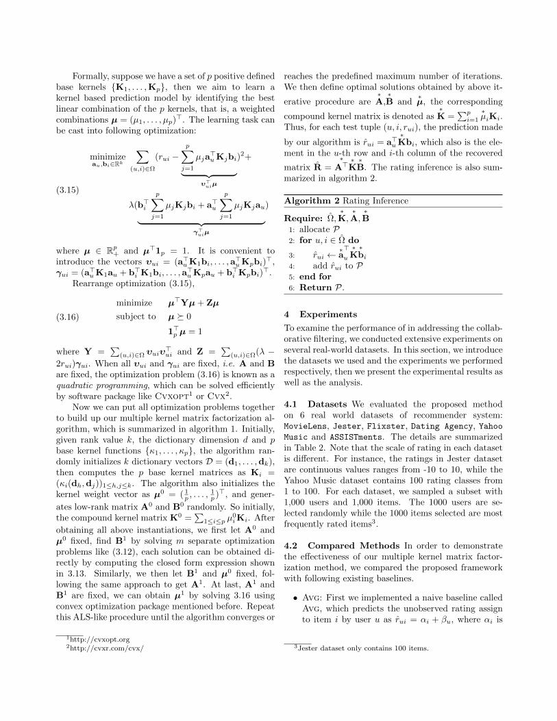
Algorithm 1 Multiple Kernel Matrix Factorization

Require: k, d, κ1, . . . , κp,R,Ω, λ, itermax1: allocate A ∈ Rk×m,B ∈ Rk×n,µ ∈ Rp,D = di ∈

Rd : 1 ≤ i ≤ k,Ki ∈ Rk×k : 1 ≤ i ≤ p,K ∈ Rk×k2: initialize µ = ( 1

p , . . . ,1p )>,A, B, D

3: for i← 1, p do4: Ki ← (κi(dh,dj))1≤h,j≤k5: end for6: iter ← 07: repeat8: K←

∑pi=1 µiKi

9: Update B as shown in (3.13)10: Update A as shown in (3.14)11: Update µ by solving (3.16)12: until iter = itermax or convergence13: Return A,B,µ,K

3.3 Multiple Kernel Matrix Factorization Mul-tiple kernel learning(MKL) [1, 5, 11] has been widelyused on improving the performance of classification andregression tasks, the basic idea of MKL is combine mul-tiple kernels instead of using a single one.

Formally, suppose we have a set of p positive definedbase kernels K1, . . . ,Kp, then we aim to learn akernel based prediction model by identifying the bestlinear combination of the p kernels, that is, a weightedcombinations µ = (µ1, . . . , µp)

>. The learning task canbe cast into following optimization:

(3.15)

minimizeau,bi∈Rk

∑(u,i)∈Ω

(rui −p∑j=1

µja>uKjbi︸ ︷︷ ︸

υ>uiµ

)2+

λ(b>i

p∑j=1

µjKjbi + a>u

p∑j=1

µjKjau︸ ︷︷ ︸γ>uiµ

)

where µ ∈ Rp+ and µ>1p = 1. It is convenient tointroduce the vectors υui = (a>uK1bi, . . . ,a

>uKpbi)

>,γui = (a>uK1au + b>i K1bi, . . . ,a

>uKpau + b>i Kpbi)

>.Rearrange optimization (3.15),

(3.16)

minimize µ>Yµ + Zµ

subject to µ 0

1>p µ = 1

where Y =∑

(u,i)∈Ω υuiυ>ui and Z =

∑(u,i)∈Ω(λ −

2rui)γui. When all υui and γui are fixed, i.e. A and Bare fixed, the optimization problem (3.16) is known as aquadratic programming, which can be solved efficientlyby software package like Cvxopt1 or Cvx2.

Now we can put all optimization problems togetherto build up our multiple kernel matrix factorization al-gorithm, which is summarized in algorithm 1. Initially,given rank value k, the dictionary dimension d and pbase kernel functions κ1, . . . , κp, the algorithm ran-domly initializes k dictionary vectors D = (d1, . . . ,dk),then computes the p base kernel matrices as Ki =(κi(dh,dj))1≤h,j≤k. The algorithm also initializes thekernel weight vector as µ0 = ( 1

p , . . . ,1p )>, and gener-

ates low-rank matrix A0 and B0 randomly. So initially,the compound kernel matrix K0 =

∑1≤i≤p µ

0iKi. After

obtaining all above instantiations, we first let A0 andµ0 fixed, find B1 by solving m separate optimizationproblems like (3.12), each solution can be obtained di-rectly by computing the closed form expression shownin 3.13. Similarly, we then let B1 and µ0 fixed, fol-lowing the same approach to get A1. At last, A1 andB1 are fixed, we can obtain µ1 by solving 3.16 usingconvex optimization package mentioned before. Repeatthis ALS-like procedure until the algorithm converges or

1http://cvxopt.org2http://cvxr.com/cvx/

reaches the predefined maximum number of iterations.We then define optimal solutions obtained by above it-

erative procedure are∗A,∗B and

∗µ, the corresponding

compound kernel matrix is denoted as∗K =

∑pi=1

∗µiKi.

Thus, for each test tuple (u, i, rui), the prediction made

by our algorithm is rui = a>u∗Kbi, which also is the ele-

ment in the u-th row and i-th column of the recovered

matrix R =∗

A>∗K∗B. The rating inference is also sum-

marized in algorithm 2.

Algorithm 2 Rating Inference

Require: Ω,∗K,∗A,∗B

1: allocate P2: for u, i ∈ Ω do

3: rui ←∗a>u

∗K∗bi

4: add rui to P5: end for6: Return P.

4 Experiments

To examine the performance of in addressing the collab-orative filtering, we conducted extensive experiments onseveral real-world datasets. In this section, we introducethe datasets we used and the experiments we performedrespectively, then we present the experimental results aswell as the analysis.

4.1 Datasets We evaluated the proposed methodon 6 real world datasets of recommender system:MovieLens, Jester, Flixster, Dating Agency, YahooMusic and ASSISTments. The details are summarizedin Table 2. Note that the scale of rating in each datasetis different. For instance, the ratings in Jester datasetare continuous values ranges from -10 to 10, while theYahoo Music dataset contains 100 rating classes from1 to 100. For each dataset, we sampled a subset with1,000 users and 1,000 items. The 1000 users are se-lected randomly while the 1000 items selected are mostfrequently rated items3.

4.2 Compared Methods In order to demonstratethe effectiveness of our multiple kernel matrix factor-ization method, we compared the proposed frameworkwith following existing baselines.

• Avg: First we implemented a naive baseline calledAvg, which predicts the unobserved rating assignto item i by user u as rui = αi + βu, where αi is

3Jester dataset only contains 100 items.

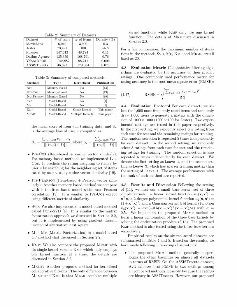
Table 2: Summary of DatasetsDataset # of users # of items Density (%)

MovieLens 6,040 3,900 6.3Jester 73,421 100 55.8Flixster 147,612 48,784 0.11Dating Agency 135,359 168,791 0.76Yahoo Music 1,948,882 98,211 0.006ASSISTments 46,627 179,084 0.073

Table 3: Summary of compared methods.

Method Type Kernelized Publication

Avg Memory-Based No [13]

Ivc-Cos Memory-Based No [19]

Ivc-Person Memory-Based No [19]

Svd Model-Based No [4]

Mf Model-Based No [9]

Kmf Model-Based Single Kernel This paper

Mkmf Model-Based Multiple Kernels This paper

the mean score of item i in training data, and βuis the average bias of user u computed as

βu =

∑(u,i)∈Ω rui − αi||(u, i) ∈ Ω||

,where αi =

∑(u,i)∈Ω rui

||(u, i) ∈ Ω||

• Ivs-Cos (Item-based + cosine vector similarly):For memory based methods we implemented Ivs-Cos. It predicts the rating assigning to item i byuser u by searching for the neighboring set of itemsrated by user u using cosine vector similarity [19].

• Ivs-Pearson (Item-based + Pearson vector simi-larly): Another memory based method we comparewith is the item based model which uses Pearsoncorrelation [19]. It is similar to Ivs-Cos exceptusing different metric of similarity.

• Svd: We also implemented a model based methodcalled Funk-SVD [4]. It is similar to the matrixfactorization approach we discussed in Section 2.2,but it is implemented by using gradient descentinstead of alternative least square.

• Mf: Mf (Matrix Factorization) is a model-basedCF method that discussed in Section 2.2.

• Kmf: We also compare the proposed Mkmf withits single-kernel version Kmf which only employsone kernel function at a time, the details arediscussed in Section 3.2.

• Mkmf: Another proposed method for kernelizedcollaborative filtering. The only difference betweenMkmf and Kmf is that Mkmf combine multiple

kernel functions while Kmf only use one kernelfunction. The details of Mkmf are discussed inSection 3.2.

For a fair comparison, the maximum number of itera-tions in the methods Svd, Mf, Kmf and Mkmf are allfixed as 20.

4.3 Evaluation Metric Collaborative filtering algo-rithms are evaluated by the accuracy of their predictratings. One commonly used performance metric forrating accuracy is the root mean square error (RMSE):

(4.17) RMSE =

√∑(u,i)∈Ω (rui − rui)2

|Ω|

4.4 Evaluation Protocol For each dataset, we se-lect the 1,000 most frequently rated items and randomlydraw 1,000 users to generate a matrix with the dimen-sion of 1000× 1000 (1000× 100 for Jester). Two exper-imental settings are tested in this paper respectively.In the first setting, we randomly select one rating fromeach user for test and the remaining ratings for training.The random selection is repeated 5 times independentlyfor each dataset. In the second setting, we randomlyselect 3 ratings from each user for test and the remain-ing ratings for training. The random selection is alsorepeated 5 times independently for each dataset. Wedenote the first setting as Leave 1, and the second set-ting as Leave 3, which has sparser training matrix thanthe setting of Leave 1. The average performances withthe rank of each method are reported.

4.5 Results and Discussion Following the settingof [11], we first use a small base kernel set of threesimple kernels: a linear kernel function κ1(x,x′) =x>x, a 2-degree polynomial kernel function κ2(x,x′) =(1 + x>x)2, and a Gaussian kernel (rbf kernel) functionκ3(x,x′) = exp(−0.5(x − x′)>(x − x′)/σ) with σ =0.5. We implement the proposed Mkmf method tolearn a linear combination of the three base kernels bysolving the optimization problem (3.15). The proposedKmf method is also tested using the three base kernelsrespectively.

Empirical results on the six real-word datasets aresummarized in Table 4 and 5. Based on the results, wehave made following interesting observations:

• The proposed Mkmf method generally outper-forms the other baselines on almost all datasetsin terms of RMSE. On the ASSISTments dataset,Avg achieves best RMSE in two settings amongall compared methods, possibly because the ratingsare binary in ASSITments. However, our proposed

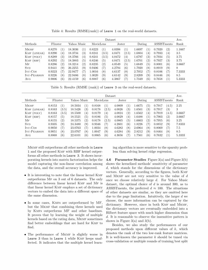
Table 4: Results (RMSE(rank)) of Leave 1 on the real-world datasets.

Dataset Ave.

Methods Flixster Yahoo Music MovieLens Jester Dating ASSISTments Rank

Mkmf 0.8270 (1) 18.3036 (1) 0.8223 (1) 4.0398 (1) 1.6697 (1) 0.7920 (2) 1.1667Kmf (linear) 0.8290 (4) 18.3734 (3) 0.8241 (3.5) 4.0471 (2.5) 1.6804 (4) 0.7933 (4) 3.5Kmf (poly) 0.8289 (3) 18.3766 (4) 0.8241 (3.5) 4.0472 (4) 1.6797 (3) 0.7934 (5) 3.75Kmf (rbf) 0.8292 (5) 18.3883 (5) 0.8246 (5) 4.0471 (2.5) 1.6701 (2) 0.7927 (3) 3.75Mf 0.8286 (2) 18.3214 (2) 0.8235 (2) 4.0549 (5) 1.6849 (5) 0.8001 (6) 3.6667Svd 0.9441 (9) 26.2255 (9) 0.9406 (7) 4.2794 (6) 1.7920 (8) 0.8919 (9) 8Ivc-Cos 0.9223 (7) 22.9477 (7) 1.0016 (8) 4.6137 (8) 2.7052 (7) 0.8106 (7) 7.3333Ivc-Pearson 0.9226 (8) 22.9486 (8) 1.0020 (9) 4.6142 (9) 2.8209 (9) 0.8446 (8) 8.5Avg 0.9006 (6) 22.4159 (6) 0.8887 (6) 4.3867 (7) 1.7349 (6) 0.7658 (1) 5.3333

Table 5: Results (RMSE (rank)) of Leave 3 on the real-word datasets.

Dataset Ave.

Methods Flixster Yahoo Music MovieLens Jester Dating ASSISTments Rank

Mkmf 0.8153 (1) 18.5034 (1) 0.8168 (1) 4.0809 (1) 1.6675 (5) 0.7917 (4.5) 2.25Kmf (linear) 0.8163 (3.5) 18.5426 (3) 0.8178 (2.5) 4.0826 (3) 1.6561 (3) 0.7917 (3) 3Kmf (poly) 0.8163 (3.5) 18.5500 (4) 0.8179 (4) 4.0824 (2) 1.6562 (4) 0.7919 (4.5) 3.6667Kmf (rbf) 0.8157 (5) 18.5521 (5) 0.8186 (5) 4.0829 (4) 1.6488 (1) 0.7903 (2) 3.6667Mf 0.8155 (2) 18.5375 (2) 0.8178 (2.5) 4.0865 (5) 1.6663 (2) 0.7955 (6) 3.25Svd 0.9335 (9) 24.3480 (9) 0.9346 (7) 4.2601 (6) 1.8226 (7) 0.8852 (9) 7.8333Ivc-Cos 0.9050 (7) 23.0763 (7) 1.0034 (8) 4.6282 (8) 2.6964 (8) 0.8069 (7) 7.5Ivc-Pearson 0.9051 (8) 23.0767 (8) 1.0047 (9) 4.6284 (9) 2.8212 (9) 0.8464 (8) 8.5Avg 0.8868 (6) 22.6101 (6) 0.8865 (6) 4.3656 (7) 1.7561 (6) 0.7632 (1) 5.3333

Mkmf still outperforms all other methods in Leave

1 and the proposed Kmf with RBF kernel outper-forms all other methods in Leave 3. It shows incor-porating kernels into matrix factorization helps themodel capturing the non-linear correlation amongthe data, and the overall accuracy is improved.

• It is interesting to note that the linear kernel Kmfoutperforms Mf on 3 out of 6 datasets. The onlydifference between linear kernel Kmf and Mf isthat linear kernel Kmf employs a set of dictionaryvectors to embed the data into a different space ofthe same dimension.

• In some cases, Kmfs are outperformed by MF,but the Mkmf that combining three kernels usedby Kmfs outperforms MF and other baselines.It proves that by learning the weight of multiplekernels based on the rating data, Mkmf sometimesfind better embeddings that are hard for Kmf tofind.

• The performance of Mkmf is slightly worse inLeave 3 than in Leave 1 while Kmf keeps unaf-fected. It indicates that the multiple kernel learn-

ing algorithm is more sensitive to the sparsity prob-lem than solving kernel ridge regression.

4.6 Parameter Studies Figure 3(a) and Figure 3(b)shows the kernelized methods’ sensitivity of parameterd, which stands for the dimensions of the dictionaryvectors. Generally, according to the figures, both Kmfand Mkmf are not very sensitive to the value of donce we choose relatively large d. For Yahoo Musicdataset, the optimal choice of d is around 300, as toASSISTments, the preferred d ≈ 100. The situationsof other datasets are similar, so they are omitted heredue to the page limitation. Intuitively, the larger d wechoose, the more information can be captured by thedictionary. However, since in both Kmf and Mkmf,the dictionary vectors are eventually embedded into aHilbert feature space with much higher dimension thand. It is reasonable to observe the insensitive pattern isshown in Figure 3(a) and 3(b).

Besides, we also study the performances of ourproposed methods upon different values of k, whichdenotes the rank of the two low-rank feature matrices.It is well-known the parameter k should be tuned viacross-validation or multiple rounds of training/test split

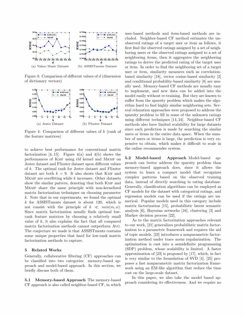
100 150 200 250 300 350 400 450 500d

18.2

18.3

18.4

18.5

18.6R

MSE

KMF(rbf)MKMF

(a) Yahoo Music Dataset

100 150 200 250 300 350 400 450 500d

0.7930

0.7935

0.7940

0.7945

0.7950

0.7955

0.7960

RM

SE

KMF(rbf)MKMF

(b) ASSISTments Dataset

Figure 3: Comparison of different values of d (dimensionof dictionary vectors)

2 4 6 8 10 12 14k

4.00

4.05

4.10

4.15

4.20

4.25

4.30

RM

SE

KMF(rbf)MKMF

(a) Jester Dataset

2 4 6 8 10 12 14k

0.82

0.83

0.84

0.85

0.86

0.87

0.88

RM

SE

KMF(rbf)MKMF

(b) Flixster Dataset

Figure 4: Comparison of different values of k (rank ofthe feature matrices)

to achieve best performance for conventional matrixfactorization [4, 15]. Figure 4(a) and 4(b) shows theperformances of Kmf using rbf kernel and Mkmf onJester dataset and Flixster dataset upon different valuesof k. The optimal rank for Jester dataset and Flixsterdataset are both k = 9. It also shows that Kmf andMkmf are overfitting while k increases. Other datasetsshow the similar pattern, denoting that both Kmf andMkmf share the same principle with non-kernelizedmatrix factorization techniques on choosing parameterk. Note that in our experiments, we found the optimalk for ASSISTments dataset is about 120, which isnot consist with the principle of k min(m,n).Since matrix factorization usually finds optimal low-rank feature matrices by choosing a relatively smallvalue of k, it also explains the fact that all comparedmatrix factorization methods cannot outperform Avg.The conjecture we made is that ASSISTments containssome unique properties that hard for low-rank matrixfactorization methods to capture.

5 Related Works

Generally, collaborative filtering (CF) approaches canbe classified into two categories: memory-based ap-proach and model-based approach. In this section, webriefly discuss both of them.

5.1 Memory-based Approach The memory-basedCF approach is also called neighbor-based CF, in which

user-based methods and item-based methods are in-cluded. Neighbor-based CF method estimates the un-observed ratings of a target user or item as follows, itfirst find the observed ratings assigned by a set of neigh-boring users or the observed ratings assigned to a set ofneighboring items, then it aggregates the neighboringratings to derive the predicted rating of the target useror item. In order to find the neighboring set of a targetuser or item, similarity measures such as correlation-based similarity [18], vector cosine-based similarity [2]and conditional probability-based similarity [8] are usu-ally used. Memory-based CF methods are usually easyto implement, and new data can be added into themodel easily without re-training. But they are known tosuffer from the sparsity problem which makes the algo-rithm hard to find highly similar neighboring sets. Sev-eral relaxation approaches were proposed to address thesparsity problem to fill in some of the unknown ratingsusing different techniques [14, 24]. Neighbor-based CFmethods also have limited scalability for large datasetssince each prediction is made by searching the similarusers or items in the entire data space. When the num-ber of users or items is large, the prediction is very ex-pensive to obtain, which makes it difficult to scale inthe online recommender system.

5.2 Model-based Approach Model-based ap-proach can better address the sparsity problem thanmemory-based approach does, since it allows thesystem to learn a compact model that recognizescomplex patterns based on the observed trainingdata, instead of directly searching in rating database.Generally, classification algorithms can be employed asCF models for the dataset with categorical ratings, andregression models can be used if the ratings are nu-merical. Popular models used in this category includematrix factorization [15], probabilistic latent semanticanalysis [6], Bayesian networks [16], clustering [3] andMarkov decision process [22].

As to the matrix factorization approaches relevantto our work, [21] generalizes probabilistic matrix factor-ization to a parametric framework and requires the aidof topic models. [23] introduces a nonparametric factor-ization method under trace norm regularization. Theoptimization is cast into a semidefinite programming(SDP) problem, whose scalability is limited. A fasterapproximation of [23] is proposed by [17], which, in factis very similar to the formulation of SVD [4]. [25] pro-poses a fast nonparametric matrix factorization frame-work using an EM-like algorithm that reduce the timecost on the large-scale dataset.

In this paper, we also take the model based ap-proach considering its effectiveness. And we require no

aid from side information to make our proposed meth-ods more generalized. To the best of our knowledge,this paper is the first work leverages both kernel meth-ods and multiple kernel learning for matrix factorizationto address the CF problem.

6 Conclusion

We have presented two novel matrix completion meth-ods named Kmf and Mkmf, which both can exploit theunderlying nonlinear correlations among rows (users)and columns (items) of the rating matrix simultane-ously. Kmf incorporates kernel methods for matrix fac-torization, which embeds the low-rank feature matricesinto a much higher dimensional space, enabling the abil-ity to learn nonlinear correlations upon the rating datain original space. Mkmf further extends Kmf to com-bine multiple kernels by learning the a set of weights foreach kernel functions based on the observed data in rat-ing matrix. As demonstrated in the experiments, ourproposed methods improve the overall performance ofpredicting the unobserved data in the matrix comparedto state-of-art baselines.

References

[1] F.R. Bach, G. Lanckriet, and M.I. Jordan. Multiplekernel learning, conic duality, and the smo algorithm.In ICML, page 6. ACM, 2004.

[2] J.S. Breese, D. Heckerman, and C. Kadie. Empiri-cal analysis of predictive algorithms for collaborativefiltering. In Proceedings of the Fourteenth conferenceon Uncertainty in artificial intelligence, pages 43–52,1998.

[3] S. Chee, J. Han, and K. Wang. Rectree: An efficientcollaborative filtering method. In Data Warehousingand Knowledge Discovery, pages 141–151. Springer,2001.

[4] S. Funk. Netflix update: Try this at home, 2006.[5] M. Gonen and E. Alpaydın. Multiple kernel learn-

ing algorithms. The Journal of Machine Learning Re-search, 12:2211–2268, 2011.

[6] T. Hofmann. Latent semantic models for collaborativefiltering. TOIS, 22(1):89–115, 2004.

[7] Y. Hu, Y. Koren, and C. Volinsky. Collaborativefiltering for implicit feedback datasets. In ICDM, pages263–272. IEEE, 2008.

[8] G. Karypis. Evaluation of item-based top-n recommen-dation algorithms. In CIKM, pages 247–254. ACM,2001.

[9] Y. Koren, R. Bell, and C. Volinsky. Matrix factoriza-tion techniques for recommender systems. Computer,(8):30–37, 2009.

[10] G. Lanckriet, T. De Bie, N. Cristianini, M.I. Jordan,and W.S. Noble. A statistical framework for genomicdata fusion. Bioinformatics, 20(16):2626–2635, 2004.

[11] G. Lanckriet, N. Cristianini, P. Bartlett, L.E. Ghaoui,and M.I. Jordan. Learning the kernel matrix withsemidefinite programming. The Journal of MachineLearning Research, 5:27–72, 2004.

[12] N.D. Lawrence and R. Urtasun. Non-linear matrixfactorization with gaussian processes. In ICML, pages601–608. ACM, 2009.

[13] C. Ma. A guide to singular value decomposition forcollaborative filtering, 2008.

[14] H. Ma, I. King, and M.R. Lyu. Effective missing dataprediction for collaborative filtering. In SIGIR, pages39–46. ACM, 2007.

[15] A. Paterek. Improving regularized singular value de-composition for collaborative filtering. In Proceedingsof KDD cup and workshop, pages 5–8, 2007.

[16] D.M. Pennock, E. Horvitz, S. Lawrence, and C.L.Giles. Collaborative filtering by personality diagnosis:A hybrid memory-and model-based approach. InProceedings of the Sixteenth conference on Uncertaintyin artificial intelligence, pages 473–480, 2000.

[17] J. Rennie and N. Srebro. Fast maximum margin matrixfactorization for collaborative prediction. In ICML,pages 713–719. ACM, 2005.

[18] P. Resnick, N. Iacovou, M. Suchak, P. Bergstrom, andJ. Riedl. Grouplens: an open architecture for collabo-rative filtering of netnews. In Proceedings of the 1994ACM conference on Computer supported cooperativework, pages 175–186. ACM, 1994.

[19] B. Sarwar, G. Karypis, J. Konstan, and J. Riedl.Item-based collaborative filtering recommendation al-gorithms. In WWW, pages 285–295. ACM, 2001.

[20] B. Scholkopf and A.J. Smola. Learning with kernels:Support vector machines, regularization, optimization,and beyond. MIT press, 2002.

[21] H. Shan and A. Banerjee. Generalized probabilisticmatrix factorizations for collaborative filtering. InICDM, pages 1025–1030. IEEE, 2010.

[22] G. Shani, R.I. Brafman, and D. Heckerman. An mdp-based recommender system. In Proceedings of the Eigh-teenth conference on Uncertainty in artificial intelli-gence, pages 453–460. Morgan Kaufmann PublishersInc., 2002.

[23] N. Srebro, J. Rennie, and T.S. Jaakkola. Maximum-margin matrix factorization. In Advances in neural in-formation processing systems, pages 1329–1336, 2004.

[24] G. Xue, C. Lin, Q. Yang, W. Xi, H. Zeng, Y. Yu, andZ. Chen. Scalable collaborative filtering using cluster-based smoothing. In SIGIR, pages 114–121. ACM,2005.

[25] K. Yu, S. Zhu, J. Lafferty, and Y. Gong. Fast nonpara-metric matrix factorization for large-scale collaborativefiltering. In SIGIR, pages 211–218. ACM, 2009.

[26] T. Zhou, H. Shan, A. Banerjee, and G. Sapiro. Ker-nelized probabilistic matrix factorization: Exploitinggraphs and side information. In SDM, volume 12,pages 403–414. SIAM, 2012.